Embed Size (px)
Citation preview

TECHNICAL UNIVERSITY - SOFIA ENGLISH LANGUAGE FACULTY OF ENGINEERING
RESEARCH PROJECT
MASTER'S DEGREE
Title: MODELLING AND SIMULATION RESEARCH ON THE METAL STRUCTURE OF BRIDGE CRANES
Supervisor Student
Assist. Prof. Ph.D. Ya. Slavchev Javier Izurriaga Lerga
SOFIA 2011

CONTENTS
1. OVERHEAD CRANES REVIEW AND CONCEPTS ..................... - 1 - 1.1. GENERAL CONSIDERATIONS ..................................................................... - 1 -
1.2. TYPES OF ELECTRIC OVERHEAD CRANES ............................................ - 1 -
1.3. EOT CRANE CONFIGURATION ................................................................... - 5 -
1.3.1. Under running cranes ................................................................................ - 5 -
1.3.2. Top Running Cranes ................................................................................. - 6 -
1.3.3. Basic crane components ............................................................................ - 6 -
1.4. ESSENTIAL PARAMETERS FOR SPECIFYING EOT CRANES ............. - 7 -
1.5. CRANE DUTY GROUPS .................................................................................. - 9 -
1.5.1. CMAA crane specification ........................................................................ - 9 -
1.5.2. FEM service class ................................................................................... - 11 -
1.6. STRUCTURAL DESIGN CONSIDERATIONS ........................................... - 12 -
1.6.1. Crane loads .............................................................................................. - 12 -
1.6.2. Rigidity requirements .............................................................................. - 13 -
1.6.3. Testing requirements ............................................................................... - 13 -
1.7. PROJECT OBJECTIVE .................................................................................. - 14 -
2. BRIDGE CRANE STRUCTURAL CALCULATIONS................. - 15 -
2.1. GENERAL CONSIDERATIONS ................................................................... - 15 -
2.2. MAIN GIRDER CALCULATIONS ............................................................... - 18 -
2.2.1. Loading evaluation .................................................................................. - 18 -
2.2.2. Main calculations. I-st calculation scheme ............................................... - 19 -
2.2.3. Calculation of local stability ................................................................... - 23 -
2.2.4. Main calculations. II-nd calculation scheme ............................................ - 25 -
2.2.5. Local stresses calculations ...................................................................... - 28 -
2.2.6. Stiffness check ........................................................................................ - 30 -
3. ABOUT THE FINITE ELEMENT METHOD ............................... - 32 - 3.1. BRIEF FEM HISTORY ................................................................................... - 32 -
3.2. GENERAL CONCEPTS .................................................................................. - 33 -
3.3. GENERAL FEA ALGORITHM ..................................................................... - 35 -
3.3.1. Preprocessing .......................................................................................... - 35 -
3.3.2. Solution ................................................................................................... - 35 -
3.3.3. Postprocessing ......................................................................................... - 36 -

3.4. FINITE ELEMENT (FE) CHARACTERISTICS ......................................... - 36 -
3.4.1. Overview ................................................................................................. - 36 -
3.4.2. The linear spring FE ................................................................................ - 36 -
3.4.3. Flexure element and beam theories ......................................................... - 39 -
3.4.4. Beam elements in ANSYS ...................................................................... - 43 -
3.4.5. 3-D solid elements ................................................................................... - 45 -
3.4.6. 3-D finite elements in ANSYS Workbench ............................................ - 46 -
4. MODELING THE METAL STRUCTURE OF OVERHEAD BRIDGE CRANE .............................................................................. - 48 -
4.1. OVERVIEW ...................................................................................................... - 48 -
4.2. 3-D BASIC CRANE MODEL (MODEL1) ..................................................... - 49 -
4.2.1. Main girders ............................................................................................ - 51 -
4.2.2. End trucks ................................................................................................ - 52 -
4.2.3. Crane driving units .................................................................................. - 55 -
4.2.4. Rails and design tables ............................................................................ - 55 -
4.3. 3-D CRANE MODEL2 AND MODEL3 ......................................................... - 57 -
4.3.1. Rimmed holes designing through sheet metal ........................................ - 60 -
5. SIMULATION RESEARCH ON THE METAL STRUCTURE OF OVERHEAD BRIDGE CRANE ...................................................... - 62 -
5.1. OVERVIEW ...................................................................................................... - 62 -
5.2. ANSYS BASIC BEAM MODEL ..................................................................... - 62 -
5.2.1. Overview ................................................................................................. - 62 -
5.2.2. Algorithm for generating the model ........................................................ - 62 -
5.2.3. Model results ........................................................................................... - 63 -
5.2.4. Validation ................................................................................................ - 64 -
5.3. 3-D BASIC MODEL SIMULATION RESEARCH. ...................................... - 67 -
5.3.1. Preparing the 3-D basic model simulation. ............................................. - 67 -
5.3.2. 3-D basic model simulation results. ........................................................ - 70 -
5.3.3. 3-D basic model vs ANSYS basic model. .............................................. - 74 -
5.3.4. 3-D basic model static structural analyses. ............................................. - 75 -
5.4. 3-D MODELS – MODEL2 AND MODEL3 STRUCTURAL ANALYSES - 92 -
5.4.1. Review ..................................................................................................... - 92 -
5.4.2. Loading case 1 ......................................................................................... - 92 -
5.4.3. Loading case 2 ....................................................................................... - 103 -

5.4.4. Loading case 3 ....................................................................................... - 105 -
5.4.5. Loading case 4 ....................................................................................... - 105 -
6. CONCLUSIONS .............................................................................. - 107 -
6.1. GENERAL OVERVIEW ............................................................................... - 107 -
6.2. COMPARISON ANALYSES......................................................................... - 107 -
6.2.1. Stress analysis ....................................................................................... - 107 -
6.2.2. Horizontal displacement analysis .......................................................... - 108 -
6.2.3. Vertical displacement analysis .............................................................. - 109 -
6.3. FINAL CONCLUSION .................................................................................. - 109 -
7. REFERENCES ................................................................................. - 112 -

- 1 -
1. OVERHEAD CRANES REVIEW AND CONCEPTS
1.1. GENERAL CONSIDERATIONS
Cranes are industrial machines that are mainly used for materials movements in construction sites, production halls, assembly lines, storage areas, power stations and similar places. Their design features vary widely according to their major operational specifications such as: type of motion of the crane structure, weight and type of the load, location of the crane, geometric features, operating regimes and environmental conditions.
When selecting an electric overhead traveling crane, there are a number of requirements to be taken into account:
1) Specifications, codes or local regulations applicable
2) Crane capacity is required
3) Required span
4) Lift required by the hoist
5) Duty cycle (usage) of the crane?
6) Hoist weight. Need for a second hoist on the bridge crane.
7) Hook approach required?
8) Desired length of runway system
9) Factors to be considered in the design of runway and building structure
10) Operating environment (dust, paint fumes, outdoor, etc)
11) Necessary crane and trolley speeds
12) Supply voltage/phases/amperage
13) Control system
14) Existing cranes on the runway
15) Category of safety considerations to be followed
16) Maintenance aspects of the crane.
17) Accessories such as lights, warning horns, weigh scales, limit switches, etc.
For high capacities, over 30 tons, usually electric overhead cranes (EOT) are the preferred type.
1.2. TYPES OF ELECTRIC OVERHEAD CRANES
There are various types of overhead cranes with many being highly specialized, but the great majority of installations fall into one of three categories:
a) Top running single girder bridge cranes
b) Top running double girder bridge cranes
c) Under-running single girder bridge cranes

- 2 -
Electric Overhead Traveling (EOT) cranes come in various types:
1) Single girder bridge cranes, Fig. 1.1 - The crane consists of a single bridge girder supported on two end trucks. It has a trolley hoist mechanism that runs on the bottom flange of the bridge girder.
Fig. 1.1 Single girder electric overhead crane
2) Double Girder Bridge Cranes, Fig. 1.2 - The crane consists of two bridge girders supported on two end trucks.
Fig. 1.2 Double girder electric overhead crane

- 3 -
The trolley runs on rails on the top of the bridge girders.
3) Gantry Cranes - These cranes are essentially the same as the regular overhead cranes except that the bridge for carrying the trolley or trolleys is rigidly supported on two or more legs running on fixed rails or other runway. These “legs” eliminate the supporting runway and column system and connect to end trucks which run on a rail either embedded in, or laid on top of the floor.
4) Monorail - For some applications such as production assembly line or service line, only a trolley hoist is required. The hoisting mechanism is similar to a single girder crane with a difference that the crane doesn’t have a movable bridge and the hoisting trolley runs on a fixed girder. Monorail beams are usually I-beams (tapered beam flanges).
Which Crane to choose – Single Girder or Double Girder
A common misconception is that double girder cranes are more durable. Per the industry standards (CMMA/DIN/FEM), both single and double girder cranes are equally rigid, strong and durable. This is because single girder cranes use much stronger girders than double girder cranes. The difference between single and double girder cranes is the effective lifting height. Generally, double girder cranes provide better lifting height. Single girder cranes cost less in many ways, only one cross girder is required, trolley is simpler, installation is quicker and runway beams cost less due to the lighter crane dead weight. The building costs are also lower.
However, not every crane can be a single girder crane. Generally, if the crane is more than 15 tonnes or the span is more than 30m, a double girder crane is a better solution.
The advantages and limitations of single / double girder cranes are as follows:
Single Girder Cranes
• Single girder bridge cranes generally have a maximum span between 5 and 15 meters with a maximum lift of 5-15 meters.
• They can handle 1-15 tonnes with bridge speeds approaching a maximum of 60 meters per minute (mpm), trolley speeds of approximately 30 mpm, and hoist speeds ranging from 3-18 mpm.
• They are candidates for light to moderate service and are cost effective for use as a standby (infrequently used) crane.
• Single girder cranes reduce the total crane cost on crane components, runway structure and building.
Double Girder Cranes
• Double girder cranes are faster, with maximum bridge speeds, trolley speeds and hoist speeds approaching 100 mpm, 45 mpm, and 18 mpm, respectively.
• They are useful cranes for a variety of usage levels ranging from infrequent, intermittent use to continuous severe service. They can lift up to 100 tonnes.
• These can be utilized at any capacity where extremely high hook lift is required because the hook can be pulled up between the girders, Fig. 1.3, the so-called general purpose cranes.
• They are also highly suitable where the crane needs to be fitted with walkways, crane lights, cabs, magnet cable reels or other special equipment, Fig. 1.4, Fig. 1.5.

- 4 -
Fig. 1.3 Double girder, general purpose EOT cranes
Fig. 1.4 Double girder, magnet EOT crane

- 5 -
Fig. 1.5 Double girder, grabbing EOT crane
1.3. EOT CRANE CONFIGURATION
1) Under Running (U/R)
2) Top Running (T/R)
1.3.1. Under running cranes
Under running or under slung cranes are distinguished by the fact that they are supported from the roof structure and run on the bottom flange of runway girders, Fig. 1.6. Under running cranes are typically available in standard capacities up to 10 tons (special configurations up to 25 tons and over 28 m spans). Under hung cranes offer excellent side approaches, close headroom and can be supported on runways hung from existing building members if adequate.
The under running crane offers the following advantages:
• Very small trolley approach dimensions meaning maximum utilization of the building's width and height.
• The possibility of using the existing ceiling girder for securing the crane track.
Following are some limitations to under running cranes :
• Hook height - Due to location of the runway beams, hook height is reduced
• Roof load - The load being applied to the roof is greater than that of a top running crane
• Lower flange loading of runway beams require careful sizing otherwise, you can "peel" the flanges off the beam

- 6 -
Fig. 1.6 Under running bridge crane
1.3.2. Top Running Cranes
The crane bridge, Fig. 1.7 travels on top of rails mounted on a runway beam supported by either the building columns or columns specifically engineered for the crane. Top Running Cranes are the most common form of crane design where the crane loads are transmitted to the building columns or free standing structure. These cranes have an advantage of minimum headroom / maximum height of lift.
Fig. 1.7 Top running bridge crane
1.3.3. Basic crane components
1) Bridge - The main traveling structure of the crane which spans the width of the bay and travels in a direction parallel to the runway. The bridge consists of two end trucks and one or two bridge girders depending on the equipment type. The bridge also supports the trolley and the hoisting mechanism, the latter used for moving up and down the load.
2) End trucks - Located on either side of the bridge, the end trucks house the wheels on which the entire crane travels. It is an assembly consisting of structural members, wheels, bearings, axles, etc., which supports the bridge girder(s) or the trolley cross member(s).

- 7 -
3) Bridge Girder(s) - The principal horizontal beam of the crane bridge which supports the trolley and is supported by the end trucks.
4) Runway - The rails, beams, brackets and framework on which the crane operates.
5) Runway Rail - The rail supported by the runway beams on which the crane travels.
6) Hoist - The hoist mechanism is a unit consisting of a motor drive, coupling, brakes, gearing, drum, ropes, and load block designed to raise, hold and lower the maximum rated load. Hoist mechanism is mounted to the trolley.
7) Trolley - The unit carrying the hoisting mechanism which travels on the bridge rails in a direction at right angles to the crane runway. Trolley frame is the basic structure of the trolley on which are mounted the hoisting and traversing mechanisms.
8) Bumper (Buffer) - An energy absorbing device for reducing impact when a moving crane or trolley reaches the end of its permitted travel, or when two moving cranes or trolleys come into contact. This device may be attached to the bridge, trolley or runway stop.
1.4. ESSENTIAL PARAMETERS FOR SPECIFYING EOT CRANES
To select the correct crane envelope that will fit in the building foot print, the user must identify and pass on some key information to the supplier, Fig. 1.8
Fig. 1.8 Parameters needed for specifying an EOT crane
1 Crane capacity (tonnes)
2 Required lifting height (m)
3 Runway height (m)
4 Clearance Required (m)
5 Building Width, Clear Span (m)
6 Building Height (m)
7 Runway Size & Length (m)
8 Hook Approach & End Approach (m)
Other Desired Information
Hoist Speed (m per minute)
Bridge Travel Speed (m per min)
Trolley Travel Speed (m per min)
Electrical Requirements (Festoon or
Conductor Bar)
Control Requirements

- 8 -
1) Crane capacity - The rated load, the crane will be required to lift. Rated load shall mean the maximum load for which a crane or individual hoist is designed and built by the manufacturer and shown on the equipment identification plate.
2) Lift height - The rated lift means the distance between the upper and lower elevations of travel of the load block and arithmetically it is usually the distance between the beam and the floor, minus the height of the hoist. This dimension is critical in most applications as it determines the height of the runway from the floor and is dependent on the clear inside height of the building. Include any slings or below the hook devices that would influence this value.
3) Runway height – The distance between the grade level and the top of the rail.
4) Clearance- The vertical distance between the grade level and the bottom of the crane girder.
5) Clear span- Distance between columns across the width of the building. Building width is defined as the distance from outside of eave strut of one sidewall to outside of eave strut of the opposite sidewall. Crane span is the horizontal center distance between the rails of the runway on which the crane is to travel. Typically distance is approximate to 500mm less than the width of the building.
How much span a crane requires depends on the crane coverage width dictated by the application. (According to the span and the maximum load handling capacity, the crane steel structure is selected to be either a single or double girder crane construction).
6) Building height- Building height is the eave height which usually is the distance from the bottom of the main frame column base plate to the top outer point of the eave strut. Eave height is the distance from the finished floor to the top outer point of the eave strut. There must be a safety distance between the top edge of the crane runway rail and the first obstacle edge in the building (for example roof beams, lights and pipes).
7) Runway length- The longitudinal run of the runway rail parallel to the length of the building.
8) Hook approaches - Maximum hook approach is the distance from the wall to the nearest possible position of the hook. The smaller the distance is, the better can the floor area be utilized. Always check which crane gives optimum hook approaches and when combined with the true lift of the hoist you can utilize most of the available floor space. This is also termed as side hook approach.
End Approach – This term describes the minimum horizontal distance, parallel to the runway, between the outermost extremities of the crane and the centerline of the hook.
9) Bridge, trolley and lift speeds - The rate at which the bridge or trolley travels or at which the hoist lifts is usually specified in meters per minute or mpm. The crane operating speeds are selected to allow safe operation whilst using the pendant. Dual operating speeds, normally a fast and slow speed with a ratio of 4:1 are commonly used but for optimum control a variable speed control system is strongly recommended.
10) Electrical Requirements - Specify the circuit voltage shall not exceed 600 volts for AC or DC current. Ideally 480 volt, 3 phase, 50 hertz for EU requirements. The runway power is usually by conductor bar and hoisting trolley by festoon cable.
11) Control Requirements - The control circuit voltage at pendant pushbuttons shall not exceed 150 volts for AC and 300 volts for DC. Other control options including radio control, free-floating pendant (festooned) or hoist-mounted pendant requirements must be stated.

- 9 -
1.5. CRANE DUTY GROUPS
Crane duty groups are set of classifications for defining the use of crane. There are several different standards where these groups are named differently. CMAA [12], FEM, ISO or HMI, ASME [14] - they all have their own classification of duty groups but are still based on the same calculations and facts. Following is a short description of what a duty group means and what it is for.
A crane duty group tells which kind of duty the crane is for; the range is from light duty up to very heavy duty. It is vital to define the needs and estimate the use because of safety reasons and for to ensure a long working life for the crane. You can't put for example a crane designed for light duty into continuous heavy-duty work.
1.5.1. CMAA crane specification
As to the types of cranes covered under [12], there are six different classifications of cranes, each dependent on duty cycle. Within the CMAA specification is a numerical method for determining exact crane class based on the expected load spectrum. Aside from this method, the different crane classifications, as generally described by CMAA, are as follows, Table 1.1.
CMAA Class
Description Details
A
Standby or Infrequent service
This service class covers cranes where precise handling of equipment at slow speeds with long idle periods between lifts. Capacity loads may be handled for initial installation of equipment and for infrequent maintenance. Typical examples are cranes used in powerhouses, public utilities, turbine rooms, motor rooms, and transformer stations. This is the lightest crane as far as duty cycle is concerned.
B
Light Service
This service class covers cranes where service requirements are light and the speed is slow. Loads vary from none to occasional full capacity. Lifts per hour would range from 2 to 5, and average 3 m per lift. Typical examples are cranes in repair shops, light assembly operations, service buildings, light warehousing, etc.
C
Moderate Service
This service covers cranes whose service requirements are deemed moderate, handling loads which average 50 percent of the rated capacity with 5 to 10 lifts per hour, averaging 4,5 m, with not over 50 percent of the lifts at rated capacity.
In terms of numbers, most cranes are built to meet class C service requirements. This service covers cranes that may be used in machine shops or paper mill machine rooms.

- 10 -
D
Heavy Service
In this type of service, loads approaching 50 percent of the rated capacity will be handled constantly during the work period. High speeds are desirable for this type of service with 10 to 20 lifts per hour averaging 4,5 m, with not over 65 percent of the lifts at rated capacity. Typical examples are cranes used in heavy machine shops, foundries, fabricating plants, steel warehouses, container yards, lumber mills, etc., and standard duty bucket and magnet operations where heavy duty production is required.
E
Severe Service
This type of service requires a crane capable of handling loads approaching the rated capacity throughout its life with 20 or more lifts per hour at or near the rated capacity. Typical examples are magnet, bucket, magnet/bucket combination cranes for scrap yards, cement mills, lumber mills, fertilizer plants, container handling, etc.
F
Continuous Severe Service
In this type of service, the crane must be capable of handling loads approaching rated capacity continuously under severe service conditions throughout its life. Typical examples are custom designed specialty cranes essential to performing the critical work tasks affecting the total production facility, providing the highest reliability with special attention to ease of maintenance features.
Table 1.1 CMAA crane specifications

- 11 -
1.5.2. FEM service class
To determine your crane duty group (according to FEM [15], [16], Fédération Européene de la Manutention) you need following factors:
1) Load spectrum (Indicates the frequency of maximum and smaller loadings during examined time period).
2) Class of utilization (This is determined according to number of hoisting cycles during lifetime of crane)
3) Combining these factors is how a duty group is selected.
Example of different load spectrums:
Fig. 1.9 FEM load spectrums

- 12 -
1.6. STRUCTURAL DESIGN CONSIDERATIONS
1.6.1. Crane loads
A crane structure is subjected to following types of loads (forces):
1) Dead Loads – A load that is applied steadily and remains in a fixed position relative to the structure. The dead load is a steady state and does not contribute to the stress range.
2) Live Load - A load which fluctuates, with slow or fast changes in magnitude relative to the structure under consideration.
3) Shock Load – A load that is applied suddenly or a load due to impact in some form.
All these loads induce various types of stresses that can be generally classified in one of four categories:
• Residual stresses – These are due to the manufacturing processes that leave stresses in a material, for example welding leaves residual stresses in the metals welded.
• Structural stresses- These are stresses produced in structural members because of the weights they support. These are found in building foundations and frameworks due to dead weight of the crane.
• Thermal stresses – These exist whenever temperature gradients are present in a material.
• Fatigue stresses – These occur due to cyclic application of a stress. These stresses could be due to vibration or thermal cycling.
Of all these stresses, the fatigue stresses demand the maximum attention. Crane runway girders are subjected to repetitive stressing and un-stressing due to number of crane passages per hour (or per day).
Since it, is not easy to estimate the number of crane passages, for design purposes it is assumed that the number of stress fluctuations corresponds to the class of the crane as specified in the codes.
When designing structures supporting crane, the main loads and forces to be considered are:
1) Vertical loads – The predominant loading on the crane supporting structure is vertical loads and is usually supplied by manufactures by way of maximum wheel loads. These loads may differ from wheel to wheel depending on the relative positions of the crane components and the lifted load
2) Side thrust lateral loads - Crane side thrust is a horizontal force of short duration applied transversely by the crane wheels to the rails. Side thrust arises from one or more of:
• Acceleration and deceleration of the crane bridge and the crab
• Impact loads due to end stops placed on the crane runway girder
• Off-vertical lifting at the start of hoisting
• Tendency of the crane to travel obliquely

- 13 -
• Skewing or crabbing of the crane caused by the bridge girders not running perpendicular to the runways. Some normal skewing occurs in all bridges.
• Misaligned crane rails or bridge end trucks
Oblique traveling of the crane can also induce lateral loads. The forces on the rail are acting in opposite directions on each wheel of the end carriage and depend on the ratio of crane span to wheel base.
3) Traction Load - Longitudinal crane traction force is of short duration, caused by crane bridge acceleration or braking.
4) Bumper Impact - This is longitudinal force exerted on the crane runway by a moving crane bridge striking the end stop.
1.6.2. Rigidity requirements
The following maximum values for the deflection of the crane girder must normally not be exceeded in order to avoid undesirable dynamic effects and to secure the function of the crane:
1) Vertical deflection is defined as the maximum permissible deflection ratio allowed for a lifting device. For bridge crane this value is usually L/700 (few specs require L/900), where L is the span of a bridge crane.
2) Horizontal deflection is a maximum deflection ratio allowed for a bridge crane or runway. This value is L/600, where L is the span of a bridge crane.
In the absence of more detailed calculations, it is acceptable to assume that the top flange resists the whole horizontal force. The rigidity requirement for horizontal deflection is essential to prevent oblique traveling of the crane. The vertical deflection is normally limited to a value not greater than 25 mm to prevent excessive vibrations caused by the crane operation and crane travel.
1.6.3. Testing requirements
Crane test loads are typically specified at 125% of rated capacity by both OSHA [13] and ASME. Neither standard, however, specify an acceptable tolerance over or under the 125% figure. The only reference to such a tolerance was given in an interpretation by ASME B30.2. Though not considered a part of the standard, this interpretation suggested a tolerance of +0%/-4% on the weight of the test load. In effect, this suggested a test load weighing between 120% and 125% of the rated crane capacity (i.e.: 125% -125% x 0.04 = 120%).
A bridge, gantry or overhead traveling crane installed after January 1, 1999, or such a crane or its runway which has been significantly modified, must be load tested before being put into service as follows:
1) All crane motions must be tested under loads of 100% and 125% of the rated capacity for each hoist on the crane, and the crane must be able to safely handle a load equal to 125% of the rated capacity;
2) All limit-switches, brakes and other protective devices must be tested when the crane is carrying 100% of the rated capacity;

- 14 -
3) Structural deflections must be measured with loads of 100% and 125% of the rated capacity and must not exceed the allowable deflections specified by the applicable design standard;
4) The load must be traveled over the full length of the bridge and trolley runways during the 100% and 125% load tests, and only the parts of runways that have been successfully load tested may be placed into service.
5) A record of all load tests must be included in the equipment record system giving details of the tests and verification of the loads used, and must be signed by the person conducting the tests.
6) A replacement crane or hoist to be installed on an existing runway may be load tested in the manufacturer's facility and installed on an existing runway provided that the replacement unit has a rated capacity and gross weight equal to or less than the previously tested rating for the runway, and the runway need not be load tested unless it has been modified since it was previously load tested.
1.7. PROJECT OBJECTIVE
The carrying metal construction is the most metal-intensive part of overhead cranes and is often subject to optimization and mass reduction.
The objective of this project is to reduce the structural mass of a real-world double girder overhead crane, produced by Kranostroene Engineering – Sofia, through the use of modern computer modeling and simulation methods and applications.
Following closely the established theoretical foundations and engineering checking schemes the structure mass reduction must be verified by structural static stress simulations.
So, for the fulfillment of the project objective, the following tasks will be completed:
- Accumulating specific awareness of modern computer modeling and simulation tools and applications, such as SolidWorks, ANSYS, Workbench and the Finite Element Method
- 3-D modeling and static structural simulations of a double girder overhead crane in order to establish its detailed 3-D structural response. This includes static stress analyses, frequency analyses, comparison with the well-known theoretical foundations and the Euler-Bernoulli formulations.
- Generating models of reduced crane mass. Perform 3-D modeling and structural simulations of the static structural response of the new designs and provide evidence that they conform to standard requirements and do not deviate significantly from the original crane response.

- 15 -
2. BRIDGE CRANE STRUCTURAL CALCULATIONS
2.1. GENERAL CONSIDERATIONS
There has been accepted a solid walled bridge construction, where main girders are welded to the end trucks. Bridge driving is by separate SEW gear units. These gear units drive the wheels placed at the side of the maintenance deck.
The major calculation pertain to double girder overhead crane 50/12,5, produced by Kranostroene Engineering – Sofia. The crane has normal duty cycle main load capacity 50 tonnes and auxiliary load capacity 12,5 tonnes. Some of the major crane parameters are listed in Table 2.1.
Crane span 28,5L m= Main girder cross-section area (+ rail)
20,05056A m=
Main girder mass 11523M kg= Crab mass (no ropes) 1 8200zM kg=
Area moment inertia of the main girder section
40,02zJ m= Crane structure
material СТ 3
Hoisting velocities Travel velocities
Main hoist 0v 0,04 /m s= Crab 2v 0,333 /m s=
Aux hoist 1v 0,233 /m s= Crane 3v 0,8 /m s=
Main hoist capacity 50Q t= Aux hoist capacity 12,5Q t=
Mode of operation Average Total bridge mass 28173kg
Table 2.1 Parameters of crane, type 50/12,5
The main dimensions are shown in Fig. 2.1 and Fig. 2.2.

- 16 -
Fig. 2.1 Metal structure with major dimensions
Bridge span is given L = 28500 mm; crab base is given M = 2850mm;
crane base B is predefined by the relation, [2], [5] etc.:
285005700 4070
5 7 5 7
LB mm≥ = = ÷
÷ ÷.
It is accepted B = 4600mm.
All other dimensions are determined by recommendatory relations in [2], [5], etc.

- 17 -
Fig. 2.2 Main girder partial view and cross section
The different elements and dimensions of the main beam are named as follows:
1 – main diaphragms; 2 – aux diaphragms; H – girder height; H1 – height of supporting cross-section; C – chamfer length; bP – flange width; δC – plate thickness; δP – flange thickness; a – main diaphragms distance; a1 – aux diaphragms distance.
1 1
16 20H L = ÷
- accepted equal to 1535mm
[ ]1 0,3 0,6H H= ÷ - accepted equal to 840mm
[ ]0,1 0,2c L= ÷ - accepted equal to 3900mm
[ ]0,55 0,33Pb H= ÷ - accepted equal to 500mm
180 240CHδ ≥÷
-accepted 8mm (at the presence of longitudinal diaphragms)
The following are accepted as:
120 ; 1845 ; 615 ;P mm a mm a mmδ = = =

- 18 -
2.2. MAIN GIRDER CALCULATIONS
Main girder calculations are performed considering the influence of constant loadings and moving loadings.
Constant loadings are: main girder weight - Ggirder as well as weights of all components connected to the girder such as – cab, deck, fences, driving units, etc.
One of the moving loadings is the crab wheels loading when the crab moves along the bridge.
There must be considered also inertia loadings due to crane starting/stopping as well as any torsion loadings. When the crane works in the open, there must be included the wind loadings.
2.2.1. Loading evaluation
Main girder weight
It is assumed to be distributed loading with intensity:
[ / ]MGq N m
Lϕ= ⋅ (2.1)
M girder deck othersG G G G= + +
3134.10girderG N= - main girder weight
320.10deckG N= - maintenance deck weight
310.10othersG N≈ - weight of fences, power supply, etc.
28,5L m= - bridge span
1,1 60 /min
1,2 60 /min
1,3 120 /min
v m
v m
v m
ϕϕ ϕ
ϕ
= → == → >= → >
-coefficients accounting for thrusts during crane motion

- 19 -
Moving loadings
These are defined according to Fig. 2.3.
Q2
KG2
Fig. 2.3 Moving loadings evaluation scheme
For general load Q position ⇒
21
12
4 2
4 2
crab
crab
G aP Q
bG a
P Qb
ψ
ψ
= + ⋅ ⋅
= + ⋅ ⋅ (2.2)
When the load Q center of mass coincides with the crab center of mass (a1 = a2 = b/2)
( )1 21
.2 4 crabR
P P G Qψ= = = + (2.3)
1,2ψ = - dynamic coefficient for normal duty cycle
2.2.2. Main calculations. I-st calculation scheme
Calculations are performed by the main calculation schemes:
I – first calculation scheme – sharp load lift at stationary crane
II – second calculation scheme – sharp stop of the crane with lifted loading
- 20 -
The I-st calculation scheme is according to Fig. 2.4.
Fig. 2.4 Main girder calculation scheme due to moving loadings
a – unequal loadings; b – equal loadings;
The max bending moment due to moving loadings is at distance B/4 to the main girder midst.
( )2
max 1
2 8.P crabb
M G Q LL
ψ = + ⋅ − ⋅
(2.4)
The max bending moment due to distributed loadings is at the span midst:
max 2
8 8M
qG Lq
M Lϕϕ ⋅ ⋅= ⋅ ⋅ = (2.5)
It could be assumed with certain approximation that both max bending moments are in the span midst. Main cross-section check (in the midst of the main girder)
There is checked the normal stress according to:
( )[ ]
2
28 8
crabM
bendingx x
bG Q L
G L
W L W
ψϕσ σ
+ ⋅ − ⋅ ⋅ = + ≤⋅ ⋅ ⋅
(2.6)

- 21 -
2. xxx
JW
H= - resistive moment.
After substitution ⇒
3 3
3 3 4
33 3
33 3
1; 164 10 ; 28,5 ; 135 10 ; =1,2;
500.10 ; 1,25 ; 1993,25 10 ; 153,5 ; 2
2 1993,25 1026 10 (rail included);
153,5
2 1593,2 1020,75 10 (ra
153,5
M crab
x x
x
x
G N L m G N
bQ N m J cm H cm
W cm
W cm
ϕ ψ
−
= = ⋅ = = ⋅
= = = ⋅ =
⋅ ⋅= = ⋅
⋅ ⋅= = ⋅
( )( )23 33I, with railbending 3 3
I, no railbending
il excluded);
135 10 1,2 500 10 2850 1251 164 10 2850
8.26.10 8 2850 26 10
114,5
143,5
MPa
MPa
σ
σ
⋅ + ⋅ ⋅ −⋅ ⋅ ⋅= + =⋅ ⋅ ⋅
=
=
[ ] 160 170I MPaσ = ÷ - [1], [17], etc. ⇒ [ ]bending Iσ σ<
• supporting cross-section check
There is checked the tangential stresses ( )zx yzτ τ caused by tangential forces ( )z yQ :
( )( )
0( ).2.z y
zx yzc
Q
h Hτ
δ= (2.7)
( )z yQ is defined for two cases:
a) When one of the crab wheels is right on the corresponding support as in Fig. 2.5.
Fig. 2.5 Calculation diagram for evaluation of tangential forces ( )( )z x yQ

- 22 -
b) Crab is in the midst as in Fig. 2.4.
First case
( )2 2 0,5
M
A zx M
LP L P L b G b
R Q P GL L
⋅ + ⋅ − + ⋅ ≡ = = − + ⋅
(2.8)
P is defined by (2.3). After substitution ⇒
( ) ( )3 3 3
(1) 3 3 3( )( )
3(1)( )( ) 3
1 1. 135 10 1,2 500 10 183,75 10 ;
4 4
2,5183,75 10 2 0,5 164.10 432,96 10
28,5
432,96 1018,1
1,495 2 8 10
crab
z x y
z x y
P G Q N
Q N
MPa
ψ
τ −
= + = ⋅ + ⋅ ⋅ = ⋅
= ⋅ ⋅ − + ⋅ = ⋅
⋅= =⋅ ⋅ ⋅
[ ] [ ]0,6 0,6 160 96I MPaτ σ= = ⋅ = .
Second case
(2) (2)3( )( ) ( )( )187,4.10 7,83z x y z x yQ N MPaτ= =

- 23 -
2.2.3. Calculation of local stability
Plates and flanges of the main and supporting cross-sections are checked for local stability. These elements are most commonly thin-walled and lose stability at a given stress value (warping, buckling). This is called loss of local stability. When local stability is lost, the corresponding zone of the plate/flange is excluded from the assembly work, leading to redistribution of stresses in the corresponding cross-section, e.g. main girder cross-section. Stresses causing local stability loss are known as critical stresses, criticalσ . These stresses
depend on many factors: contour joining, stress state characteristics, etc.
• Local stability check of the wall of the main girder midst cross-section.
The wall is assumed to be a plate, fixed at both ends as shown below:
Fig. 2.6 Diagram for checking the local stability of the main girder wall
Critical stresses are calculated as:
24
0
630 10critical MPaH
δσ
= ⋅
(2.9)
After substituting 08 ; 1495mm H mmδ = = ⇒
248
630 10 180,181495critical MPaσ = ⋅ =
The safety coefficient is: [ ]180,181,85
97,6criticalIbending
K Kσσ
= = = >
The smallest allowable value is [ ] 1,3K = , [18] etc.

- 24 -
• Stability check for the wall next to the support cross-section
Stability is checked for tangential stresses:
2 2
31250 950 10 [ ]criticalh
MPaa h
δτ = + ⋅
(2.10)
Calculation diagram is as shown below.
1845
1172
8
a mm
h mm
mmδ
===
Fig. 2.7 Diagram for checking the local stability of wall next to support cross-section
After substitution in (2.10) ⇒
2 231172 8
1250 950 10 30,61845 1845critical MPaτ
= + ⋅ =
The safety coefficient is:
[ ](1)
30,61,7 1,3
18,1criticalK K
ττ
= = = > =
• Stability check for the top flange
Flange is assumed as a plate fixed at both ends. In order to fulfill the local stability requirement ⇒
0 23081
P s
b
δ σ≤ (2.11)
Assuming that 260s MPaσ = - yield strength limit for constructional steels, regular
quality ⇒ 0 4446,3
70 70Pb
mmδ ≥ ≈ = . It is accepted that the thickness is 20P mmδ = .
- 25 -
2.2.4. Main calculations. II-nd calculation scheme
Calculations proceed in the same way as shown in Fig. 2.4. The difference, here is that loadings are applied in the vertical and horizontal planes.
• Loadings in vertical plane
( )1 21
; 4
Mv crab
Gq P P G Q
Lϕ= = = + (2.12)
( ) 211
; 8 2 4 2V
crabMq P
G QG L bM M L
Lϕ
+⋅ = ⋅ = ⋅ − ⋅ (2.13)
( )2
1
,max 28 8
crabVbending
bG Q L
G LM
L
ϕ + − ⋅ ⋅ = +
⋅ (2.14)
maxbendingII
bendingx
M
Wσ = (2.15)
• Loadings in horizontal plane
When the crane or the crab starts/stops in the regular way, certain inertia forces arise that bring additional loading to the construction.
Inertia forces could be calculated as follows:
inertia aveG
P ag
= ⋅ (2.16)
avea is the average acceleration.
Horizontal forces, in practice, are assumed as 0,1 of the corresponding concentrated loadings or distributed loadings. In the spot, where crab wheel and rail meet, some concentrated forces are expected to occur:
,1 ,2 10,1inertia inertiaF F P= = ⋅ (2.17)
Bending moment is:
( ) max, 0,1 ( )F
bendingbending inertiaM M P= ⋅ (2.18)

- 26 -
Inertia force due to girder weight, respectively inertia moment, is defined in the same way:
( ) max, 0,1 ( )q
bendingbending inertiaM M q= ⋅ (2.19)
Crab motion, starting/stopping is a source of inertia forces T that act along the main girders axis.
Normal stresses are:
( ) ( )max, ,
F qbending bending inertia bending inertia
x y
M MM
W Wτσ+
= ± (2.20)
Corner points’ stresses turn out to have max values.
Stress distribution is shown in Fig. 2.8.
Fig. 2.8 Main girder stresses
After substituting parameter values in (2.13), (2.14), (2.17), (2.18) and (2.19) ⇒
3 3 4max 3
( ) 3 3, ,
( )
( )
1,1 164 10 2850 635 10 742,5 10271059,5 10 . ;
8 8 2850
20679,2 10 . ; 6426,8 10 . ;
104,25 41,06 145,31 (rail included);
130,6 41,
bending
F qbending inertia bending inertia
z
z
M N cm
M N cm M N cm
MPaσ
σ
⋅ ⋅ ⋅ ⋅ ⋅ ⋅= + = ⋅⋅
= ⋅ = ⋅
= + =
= + 06 171,7 (rail not included);MPa=
[ ] 180MPaσ =

- 27 -
• Torsion
Max torsion stress in random torsion of a closed box is defined according to Bredt’s formula, that could be presented in the following way for support cross-sections:
max 2torsion
torsiont
M
Wτ =
⋅ (2.21)
Indexes follow Fig. 2.8.
2t b CT CTW b h δ= ⋅ ⋅ ⋅ - resistive characteristics
max torsionτ - is in the wall midst – Fig. 2.8.
3
0
2.44,4 81,2 0,8 5768,4
2
t
torsion inertia inertia
W cm
hM q L e P
= ⋅ ⋅ =
= ⋅ ⋅ − ⋅
Fig. 2.9 Inertia loading in the main girder
a)supported cross section; b) main cross- section
( )
( ) ( )
3
31
0 0
ma
0,1 164 100,1. 0,1 0,57 / ;
28501 1
0,1 2 0,1 2 0,1 635 10 31,71 ;4 2
1 1149,5 81,2 34,15 ; 81,2 ;
2 2
0,57 2850 34,15 31,75 81,2 202333,4 . ;
Minertia v
inertia crab
torsion
Gq q kg cm
L
P P G Q N
e H h cm h cm
M kg cm
⋅ ⋅= = ⋅ = =
= ⋅ ⋅ = ⋅ ⋅ + = ⋅ ⋅ ⋅ =
= − = − = =
= ⋅ ⋅ − ⋅ =
2x
202333,417,53 / 1,75
2 5768,4torsion kg cm MPaτ = = =⋅

- 28 -
Equivalent tangential stress in support cross-section is defined as a sum of shear and torsion stresses:
[ ] [ ]max max 18,1 1,75 19,85 ;
0,6 0,6 180 108
I IIeq zy torsion
II
MPa
MPa
τ τ τ
τ σ
= + = + =
= ⋅ = ⋅ =
2.2.5. Local stresses calculations
Local stresses arise in the spots where concentrated loadings are applied. When crab moves, crab wheels act upon the rail and from the rail the action is transferred to the top flange.
In cases of box type girders with rails in the midst of the cross-section, local stresses in the flange plate are defined as:
, 2
, 2
6
6
local x xp
local y yp
Fc
Fc
σδ
σδ
⋅=
⋅= ±
∓
(2.22)
F - force deforming the flange plate; ,x yc c - coefficients;
pδ - flange thickness
The calculation diagram is shown in Fig. 2.10.
Fig. 2.10 Diagram for calculating local stresses
Rail is assumed as a beam with supports at the diaphragms and the flange – a plate in random contact with the contour.

- 29 -
1 bwhen a b>
2
13 3
01
961 b P
p
PF
b J c
ca δ
=⋅ ⋅+ ⋅
⋅
(2.23)
P - loading of the wheel; pJ - rail inertia moment;
1 1
0 b
c ak f
c b
→ =
- coefficient;
( )
( )( )
3 41 2
11 1
3
2
3 3
1
1. 183,75 10 ; 1083 ;
4
44,4 ; 61,5 ; 2 ; 1,4 0,1621
183,75 109743 ;
96 44,4 10831 0,1621
61,5 2
2 5 2 12 50,653;
44,4
61,51,385;
44,4
crab p
b pb
p p
b b
b
P P P G Q N J cm
ab cm a cm cm k
b
F N
a h
b b
a
b
ψ
δ
= = = + = ⋅ =
= = = ≈ ⇒ =
⋅= =⋅ ⋅
+ ⋅⋅
⋅ + ⋅ += = =
= ≈ 12 0,27
44,4p
b
b
b= =
1
,
,
, , , 0,1; 0,15;
6.97430,1 14,61 ;
46.9743
0,16 23,38 ;4
p px y
b b b
local x
local y
a bac f c
b b b
MPa
MPa
σ
σ
= ≈ ≈
= =
= =
∓ ∓
∓ ∓
( ) ( ) [ ]2 2, , , ,eq x local x local y x local x local yσ σ σ σ σ σ σ σ= + + − + ⋅ ≤ (2.24)
( ) ( )2 2143,5 14,61 23,38 143,5 14,61 23,38
148 160 (with no rail)
eq
eq MPa MPa
σ
σ
= + + − + ⋅ ⇒
= ≤
- 30 -
2.2.6. Stiffness check
There are made two stiffness checks – static and dynamic.
Static check verifies max static deflection f of the construction under static loading of actual load and crab:
( ) [ ]
3
2.48crabQ G L
f fE J
+ ⋅= <
⋅ ⋅ (2.25)
[ ]Q N - load capacity; [ ]crabG N - crab weight; [ ]L m - bridge span;
[ ]E Pa - Young’s modulus; 4[ ]J m - inertia moment of the main girder cross-
section;
[ ]700
Lf = - allowable deflection of overhead cranes for duty cycles 7 8,k k .
After substitution⇒ 2850
[ ] 4,07700
f cm= = ;
( )33 9
6 3
max
63,5.10 2,85 103,65 (rail included);
96 2,1 10 1993,25 10
4,04 (rail not included);
f cm
f cm
⋅ ⋅= =
⋅ ⋅ ⋅ ⋅
≈
Dynamic stiffness check is reduced to evaluating the natural frequency νννν and oscillations decay time t. Assuming one-mass-model ⇒
( ) [ ]ln 2.12 20
.
1
2.
ft t s
c
m
ν δ
νπ
= ≤ = ÷
= (2.26)
[ ]f mm - max static deflection; [ ]Hzν - natural frequency;
0,1δ = - the logarithmic decay for relation 1 1
16 18
H
L= ÷
[ ]/c N m - construction stiffness; [ ]m kg - reduced mass of the construction
3
48 17;
35 2girder crab
G GE Jc m
q gL
⋅ ⋅= = +⋅
(2.27)

- 31 -
3 3134 10 (rail included); 119 10 (rail not inlcuded);girder girderG N G N= ⋅ = ⋅
3135 10crabG N= ⋅ - crab weight; 3134 10girderG N= ⋅ - girder weight;
After substitution:
( )11 3 8
3 33
3 33 3
3
3
48 2,1 10 1593 10 106936 10 / ; 8678 10 ;
28,5
17 134.10 135.1013,5 10 ; 12,77 10 ;
35 9,81 2 9,81
1 8678 104,03 ; 3,76 ;
6,28 13,5 10
ln
rail rail
rail rail
rail rail
rail
c N m c N
m kg m kg
Hz Hz
t
ν ν
−− +
+ −
+ −
+
⋅ ⋅ ⋅ ⋅ ⋅= = ⋅ = ⋅
= ⋅ + = ⋅ = ⋅⋅
⋅= = =⋅
= (2 3,65) ln(2 41)10,64 ; 11,72 ;
4,03 0,1 3,76 0,1rails t s−⋅ ⋅= = =
⋅ ⋅

- 32 -
3. ABOUT THE FINITE ELEMENT METHOD
3.1. BRIEF FEM HISTORY
The mathematical roots of the finite element method dates back at least a half century. Approximate methods for solving differential equations using trial solutions are even older in origin. Lord Rayleigh and Ritz used trial functions (interpolation functions) to approximate solutions of differential equations. Galerkin used the same concept for solution. The drawback in the earlier approaches, compared to the modern finite element method, is that the trial functions must apply over the entire domain of the problem of concern.
While the Galerkin method provides a very strong basis for the finite element method, not until the 1940s, when Courant introduced the concept of piecewise-continuous functions in a subdomain, did the finite element method have its real start.
In the late 1940s, aircraft engineers were dealing with the invention of the jet engine and the needs for more sophisticated analysis of airframe structures to withstand larger loads associated with higher speeds. These engineers, without the benefit of modern computers, developed matrix methods of force analysis, collectively known as the flexibility method, in which the unknowns are the forces and the knowns are displacements. The finite element method, in its most often-used form, corresponds to the displacement method, in which the unknowns are system displacements in response to applied force systems.
The term displacement is quite general in the finite element method and can represent physical displacement, temperature, or fluid velocity, for example.
The term finite element was first used by Clough in 1960 in the context of plane stress analysis and has been in common usage since that time.
During the decades of the 1960s and 1970s, the finite element method was extended to applications in plate bending, shell bending, pressure vessels, and general three-dimensional problems in elastic structural analysis as well as to fluid flow and heat transfer. Further extension of the method to large deflections and dynamic analysis also occurred during this time period.
The finite element method is computationally intensive, owing to the required operations on very large matrices. In the early years, applications were performed using mainframe computers, which, at the time, were considered to be very powerful, high-speed tools for use in engineering analysis.
During the 1960s, the finite element software code NASTRAN was developed in conjunction with the space exploration program of the United States. NASTRAN was the first major finite element software code. It was, and still is, capable of hundreds of thousands of degrees of freedom (nodal field variable computations). In today’s computational environment, most of these packages can be used on desktop computers and engineering workstations to obtain solutions to large problems in static and dynamic structural analysis, heat transfer, fluid flow, electromagnetics, and seismic response.

- 33 -
3.2. GENERAL CONCEPTS
The finite element method (FEM), sometimes referred to as finite element analysis (FEA), is a computational technique used to obtain approximate solutions of boundary value problems in engineering. Simply stated, a boundary value problem is a mathematical problem in which one or more dependent variables must satisfy a differential equation everywhere within a known domain of independent variables and satisfy specific conditions on the boundary of the domain. Boundary value problems are also sometimes called field problems. The field is the domain of interest and most often represents a physical structure.
The field variables are the dependent variables of interest governed by the differential equation. The boundary conditions are the specified values of the field variables (or related variables such as derivatives) on the boundaries of the field.
Depending on the type of physical problem being analyzed, the field variables may include physical displacement, temperature, heat flux, and fluid velocity to name only a few.
Common FEA techniques and terminology could be introduced with Fig. 3.1
Fig. 3.1 FEA general terminology scheme
(a) 2-D domain of a field variable; (b) 3-node finite element (FE) in the 2-D domain;
(c) 3-node elements in a partial mesh in the 2-D domain
The figure shows a part of the volume of some material with known physical properties. The elliptical surrounding is the domain of a boundary value problem to be solved. For simplicity, at this point, we assume a two-dimensional (2-D) case with a single field variable ϕ(x, y) to be determined at every point P(x, y) such that a known governing equation (or equations) is satisfied exactly at every such point.
It means that an exact math solution is obtained, i.e. the solution is a closed-form algebraic expression of the independent variables. In practical problems, however, the

- 34 -
domain is geometrically quite complex and it is impossible to obtain a closed-form solution. Therefore, approximate solutions based on numerical techniques and digital computations are most often obtained in engineering analyses of complex problems. FEA is a powerful technique for obtaining such approximate solutions with good accuracy.
A small triangular finite element that encloses a finite-sized sub-domain of the area of interest is shown in Fig. 3.1b. Since this is a 2-D problem, it is assumed that the thickness along z-axis is constant and z dependency is not indicated in the differential equation. The vertices of the triangular element are numbered to indicate that these points are nodes. A node is a specific point in the finite element at which the value of the field variable is to be explicitly calculated. Exterior nodes are located on the boundaries of the finite element and may be used to connect an element to adjacent finite elements. Nodes that do not lie on element boundaries are interior nodes and cannot be connected to any other element.
The values of the field variable computed at the nodes are used to approximate the values at nonnodal points (that is, in the element interior) by interpolation of the nodal values. For the three-node triangle example, the nodes are all exterior and, at any other point within the element, the field variable is described by the approximate relation:
( ) ( ) ( ) ( )1 1 2 2 3 3, , , ,x y N x y N x y N x yϕ ϕ ϕ ϕ= + + (2.28)
where 1ϕ , 2ϕ and 3ϕ are the values of the field variable at the nodes, and N1, N2,
and N3 are the interpolation functions, also known as shape functions. In the finite element approach, the nodal values of the field variable are treated as unknown constants that are to be determined. The interpolation functions are most often polynomial forms of the independent variables, derived to satisfy certain required conditions at the nodes.
The interpolation functions are predetermined, known functions of the independent variables; and these functions describe the variation of the field variable within the finite element. The triangular element described by equation (2.28) is said to have 3 degrees of freedom, as three nodal values of the field variable are required to describe the field variable everywhere in the element. This would be the case if the field variable represents a scalar field, such as temperature in a heat transfer problem.
If the domain of Fig. 3.1 represents a thin, solid body subjected to plane stress, the field variable becomes the displacement vector and the values of two components must be computed at each node. In the latter case, the three-node triangular element has 6 degrees of freedom.
In general, the number of degrees of freedom associated with a finite element is equal to the product of the number of nodes and the number of values of the field variable (and possibly its derivatives) that must be computed at each node.
As depicted in Fig. 3.1c, every element is connected at its exterior nodes to other elements. The finite element equations are formulated such that, at the nodal connections, the value of the field variable at any connection is the same for each element connected to the node. Thus, continuity of the field variable at the nodes is ensured. In fact, finite element formulations are such that continuity of the field variable across inter-element boundaries is also ensured.
This feature avoids the physically unacceptable possibility of gaps or voids occurring in the domain. In structural problems, such gaps would represent physical separation of the material.

- 35 -
Although continuity of the field variable from element to element is inherent to the finite element formulation, inter-element continuity of gradients (i.e., derivatives) of the field variable does not generally exist. This is a critical observation. In most cases, such derivatives are of more interest than are field variable values. For example, in structural problems, the field variable is displacement but the true interest is more often in strain and stress.
As strain is defined in terms of first derivatives of displacement components, strain is not continuous across element boundaries. However, the magnitudes of discontinuities of derivatives can be used to assess solution accuracy and convergence as the number of elements is increased.
3.3. GENERAL FEA ALGORITHM
Certain steps in formulating a finite element analysis of a physical problem are common to all such analyses, whether structural, heat transfer, fluid flow, or some other problem. These steps are embodied in commercial finite element software packages, such as ANSYS, Workbench, etc.
The steps are as follows.
3.3.1. Preprocessing
The preprocessing step is, quite generally, described as defining the model and includes
Define the geometric domain of the problem.
Define the element type(s) to be used.
Define the material properties of the elements.
Define the geometric properties of the elements (length, area, and the like).
Define the element connectivities (mesh the model).
Define the physical constraints (boundary conditions).
Define the loadings.
The preprocessing (model definition) step is critical. In no case is there a better example of the computer-related axiom “garbage in, garbage out.” A perfectly computed finite element solution is of absolutely no value if it corresponds to the wrong problem.
3.3.2. Solution
During the solution phase, finite element software assembles the governing algebraic equations in matrix form and computes the unknown values of the primary field variable(s). The computed values are then used by back substitution to compute additional, derived variables, such as reaction forces, element stresses, and heat flow.
As it is not uncommon for a finite element model to be represented by tens of thousands of equations, special solution techniques are used to reduce data storage requirements and computation time. For static, linear problems, a wave front solver, based on Gauss elimination, is commonly used.

- 36 -
3.3.3. Postprocessing
Analysis and evaluation of the solution results is referred to as postprocessing. Postprocessor software contains sophisticated routines used for sorting, printing, and plotting selected results from a finite element solution. Examples of operations that can be accomplished include
Sort element stresses in order of magnitude.
Check equilibrium.
Calculate factors of safety.
Plot deformed structural shape.
Animate dynamic model behavior.
Produce color-coded temperature plots.
While solution data can be manipulated many ways in postprocessing, the most important objective is to apply sound engineering judgment in determining whether the solution results are physically reasonable.
3.4. FINITE ELEMENT (FE) CHARACTERISTICS
3.4.1. Overview
The primary characteristics of a finite element are embodied in the element stiffness matrix. For a structural finite element, the stiffness matrix contains the geometric and material behavior information that indicates the resistance of the element to deformation when subjected to loading.
Such deformation may include axial, bending, shear, and torsional effects. For finite elements used in nonstructural analyses, such as fluid flow and heat transfer, the term stiffness matrix is also used, since the matrix represents the resistance of the element to change when subjected to external influences.
As mentioned, the basic premise of the finite element method is to describe the continuous variation of the field variable (physical displacement) in terms of discrete values at the finite element nodes. In the interior of a finite element, as well as along the boundaries (applicable to two- and three-dimensional problems), the field variable is described via interpolation functions that must satisfy prescribed conditions.
Finite element analysis is based, dependent on the type of problem, on several mathematic/physical principles such as static equilibrium and others.
3.4.2. The linear spring FE
A linear elastic spring is a mechanical device capable of supporting axial loading only and constructed such that, over a reasonable operating range (meaning extension or compression beyond undeformed length), the elongation or contraction of the spring is directly proportional to the applied axial load. The constant of proportionality between deformation and load is referred to as the spring constant, spring rate, or spring stiffness, generally denoted as k, and has units of force per unit length. Formulation of the linear spring as a finite element is accomplished with reference to Fig. 3.2.

- 37 -
Fig. 3.2 Liner spring as a finite element
(a) nodes, nodal displacements and forces; (b) load-deformation curve
As an elastic spring supports axial loading only, an element coordinate system is defined, known also as a local coordinate system with the x-axis along the length of the spring. The element coordinate system is embedded in the element and chosen, by geometric convenience, for simplicity in describing element behavior. The element or local coordinate system is contrasted with the global coordinate system. The global coordinate system is that system in which the behavior of a complete structure is to be described. By complete structure is meant the assembly of many finite elements (several springs) for which it is required to compute the response to loading conditions. In some cases, the local and global coordinate systems are essentially the same except for translation of origin. In two- and three-dimensional cases, however, the distinctions are quite different and require mathematical rectification of element coordinate systems to a common basis. The common basis is the global coordinate system.
As shown in Fig. 3.2, the ends of the spring are the nodes and the nodal displacements are denoted by u1 and u2 and are shown in the positive sense. If these nodal displacements are known, the total elongation or contraction of the spring is known as is the net force in the spring. At this point forces are to be applied to the element, only at the nodes, and these are denoted as f1 and f2 and are also shown in the positive sense. Assuming that both the nodal displacements are zero when the spring is undeformed, the net spring deformation is given by
2 1u uδ = − (2.29)
and the resultant axial force in the spring is
( )2 1f k k u uδ= = − (2.30)
For equilibrium, f1 + f2 = 0 or f1 = −f2, and Equation (2.30) could be rewritten in terms of the applied nodal forces as
( )1 2 1f k u u= − − (2.31)
( )2 2 1f k u u= − (2.32)
which can be expressed in matrix form as
- 38 -
1 1
2 2
u fk k
u fk k
− = −
(2.33)
or
[ ]{ } { }ek u f= (2.34)
where
[ ]e
k kk
k k
− = −
(2.35)
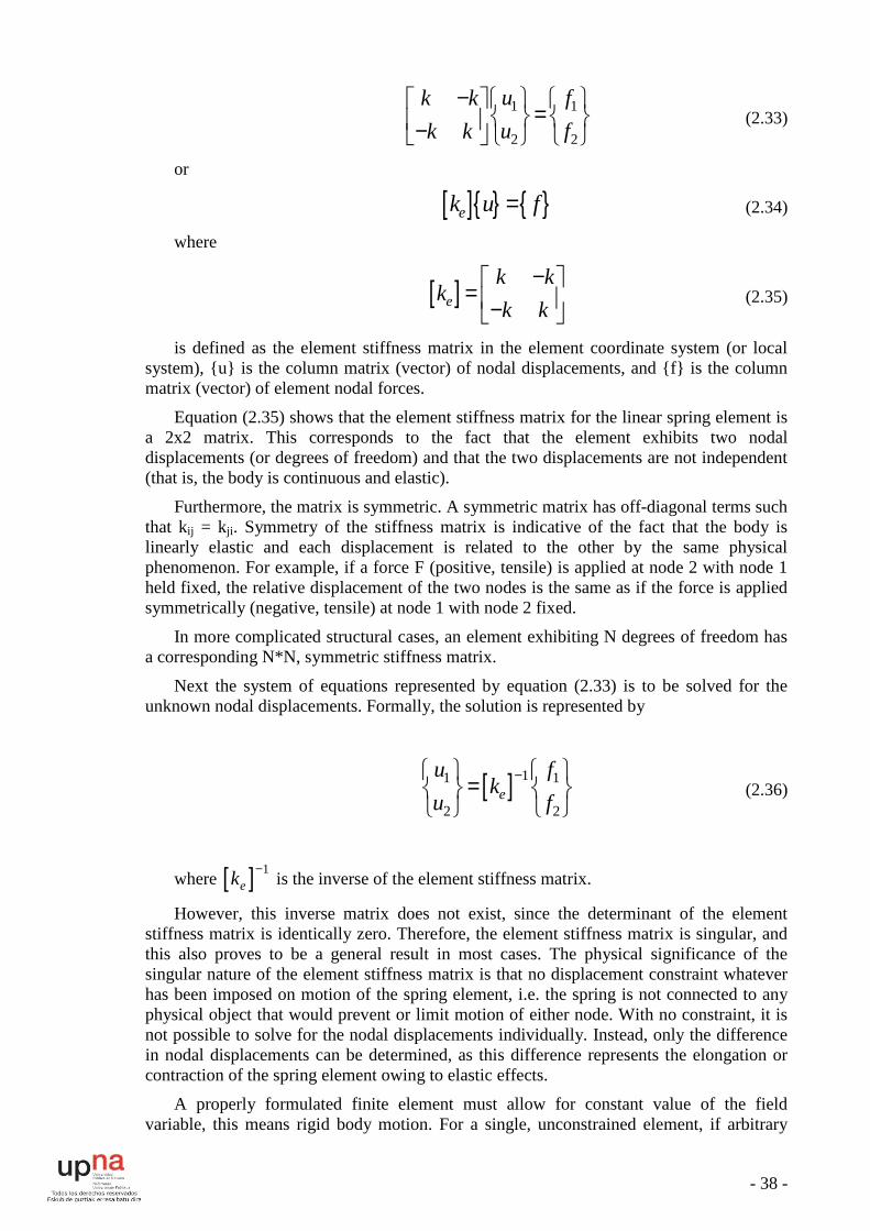
is defined as the element stiffness matrix in the element coordinate system (or local system), {u} is the column matrix (vector) of nodal displacements, and {f} is the column matrix (vector) of element nodal forces.
Equation (2.35) shows that the element stiffness matrix for the linear spring element is a 2x2 matrix. This corresponds to the fact that the element exhibits two nodal displacements (or degrees of freedom) and that the two displacements are not independent (that is, the body is continuous and elastic).
Furthermore, the matrix is symmetric. A symmetric matrix has off-diagonal terms such that kij = kji. Symmetry of the stiffness matrix is indicative of the fact that the body is linearly elastic and each displacement is related to the other by the same physical phenomenon. For example, if a force F (positive, tensile) is applied at node 2 with node 1 held fixed, the relative displacement of the two nodes is the same as if the force is applied symmetrically (negative, tensile) at node 1 with node 2 fixed.
In more complicated structural cases, an element exhibiting N degrees of freedom has a corresponding N*N, symmetric stiffness matrix.
Next the system of equations represented by equation (2.33) is to be solved for the unknown nodal displacements. Formally, the solution is represented by
[ ] 11 1
2 2e
u fk
u f−
=
(2.36)
where [ ] 1ek
− is the inverse of the element stiffness matrix.
However, this inverse matrix does not exist, since the determinant of the element stiffness matrix is identically zero. Therefore, the element stiffness matrix is singular, and this also proves to be a general result in most cases. The physical significance of the singular nature of the element stiffness matrix is that no displacement constraint whatever has been imposed on motion of the spring element, i.e. the spring is not connected to any physical object that would prevent or limit motion of either node. With no constraint, it is not possible to solve for the nodal displacements individually. Instead, only the difference in nodal displacements can be determined, as this difference represents the elongation or contraction of the spring element owing to elastic effects.
A properly formulated finite element must allow for constant value of the field variable, this means rigid body motion. For a single, unconstrained element, if arbitrary
- 39 -
forces are applied at each node, the spring not only deforms axially but also undergoes acceleration according to Newton’s second law. Hence, there exists not only deformation but overall motion. If, in a connected system of spring elements, the overall system response is such that nodes 1 and 2 of a particular element displace the same amount, there is no elastic deformation of the spring and therefore no elastic force in the spring. This physical situation must be included in the element formulation. The capability is indicated mathematically by singularity of the element stiffness matrix. As the stiffness matrix is formulated on the basis of deformation of the element, we cannot expect to compute nodal displacements if there is no deformation of the element.
Equation (2.36) indicates the mathematical operation of inverting the stiffness matrix to obtain solutions. In the context of an individual element, the singular nature of an element stiffness matrix precludes this operation, as the inverse of a singular matrix does not exist. The general solution of a finite element problem, in a global, as opposed to element, context, involves the solution of equations of the form of equation(2.34). For realistic finite element models, which are of huge dimension in terms of the matrix order (NxN) involved, computing the inverse of the stiffness matrix is a very inefficient, time-consuming operation, which should not be undertaken except for the very simplest of systems. Other, more-efficient solution techniques are available.
Derivation of the element stiffness matrix for a spring element was based on equilibrium conditions. The same procedure can be applied to a connected system of spring elements by writing the equilibrium equation for each node. However, rather than drawing free-body diagrams of each node and formally writing the equilibrium equations, the nodal equilibrium equations can be obtained more efficiently by considering the effect of each element separately and adding the element force contribution to each nodal equation. The process is described as assembly, as we take individual stiffness components and “put them together” to obtain the system or global equations.
3.4.3. Flexure element and beam theories
The one-dimensional, axial load-only elements are quite useful in analyzing the response to load of many simple structures. However, the restriction that these elements are not capable of transmitting bending effects precludes their use in modeling more commonly encountered structures that have welded or riveted joints.
The elementary beam theory is applied to develop a flexure (beam) element capable of properly exhibiting transverse bending effects.
Euler-Bernoulli beam theory, elementary beam theory, or just beam theory, is a simplification of the linear isotropic theory of elasticity which provides a means of calculating the load-carrying and deflection characteristics of beams. It was first enunciated about 1750, but was not applied on a large scale until the development of the Eiffel Tower and the Ferris Wheel in the late 19th century. Following these successful demonstrations, it quickly became a cornerstone of engineering and an enabler of the second industrial revolution.
Additional analysis tools have been developed such as plate theory and finite element analysis, but the simplicity of beam theory makes it an important tool in the sciences, especially structural and mechanical engineering.
The prevailing consensus is that Galileo Galilei made the first attempts at developing a theory of beams, but recent studies argue that Leonardo Da Vinci was the first to make the crucial observations. Da Vinci lacked Hooke's law and calculus to complete the theory, whereas Galileo was held back by an incorrect assumption he made.

- 40 -
The Bernoulli beam is named after Jacob Bernoulli, who made the significant discoveries. Leonhard Euler and Daniel Bernoulli were the first to put together a useful theory about 1750. At the time, science and engineering were generally seen as very distinct fields, and there was considerable doubt that a mathematical product of academia could be trusted for practical safety applications. Bridges and buildings continued to be designed by precedent until the late 19th century, when the Eiffel Tower and Ferris wheel demonstrated the validity of the theory on large scales.
The Euler-Bernoulli Beam Equation is based on 5 assumptions about a bending beam:
1. Calculus is valid and is applicable to bending beams;
2. The stresses in the beam are distributed in a particular, mathematically simple way;
3. The force that resists the bending depends on the amount of bending in a particular, mathematically simple way;
4. The material behaves the same way in every direction; i.e. material is isotropic.
5. The forces on the beam only cause the beam to bend, but not twist or stretch; i.e. the case is uncoupled.
More rigorously stated, these assumptions are:
1. Continuum mechanics is valid for a bending beam
2. The stress at a cross section varies linearly in the direction of bending, and is zero at the centroid of every cross section
3. The bending moment at a particular cross section varies linearly with the second derivative of the deflected shape at that location
4. The beam is composed of an isotropic material
5. The applied load is orthogonal to the beam's neutral axis and acts in a unique plane.
With these assumptions, we can derive the following equation governing the relationship between the beam's deflection and the applied load.
2 2
2 2
uEJ w
x x
∂ ∂ = ∂ ∂ (2.37)
This is the Euler-Bernoulli equation. The curve u(x) describes the deflection u of the beam at some position x (the beam is modeled as a one-dimensional object), w is a distributed load, in other words a force per unit length (analogous to pressure being a force per area); it may be a function of x, u, or other variables.
The parameter E is the elastic modulus and J is the second moment of area. The parameter J must be calculated with respect to the centroidal axis perpendicular to the applied loading. Often, u = u(x), w = w(x), and EJ is a constant, so that:
( )4
4
d uEJ w x
dx= (2.38)
This equation, describing the deflection of a uniform, static beam, is very common in engineering practice. Successive derivatives of u have important meanings:
u is the deflection

- 41 -
u
x
∂∂ is the slope of the beam
2
2
uEJ
x
∂∂ is the beam bending moment
2
2
uEJ
x x
∂ ∂− ∂ ∂ is the shear force in the beam
Besides deflection, the beam equation describes forces and moments and can thus be used to describe stresses. For this reason, the Euler-Bernoulli beam equation is widely used in engineering, especially civil and mechanical, to determine the strength (as well as deflection) of beams under bending.
Both the bending moment and the shear force cause stresses in the beam. The stress due to shear force is maximum along the neutral axis of the beam, and the maximum tensile stress is at either the top or bottom surfaces. Thus the maximum principal stress in the beam may be neither at the surface nor at the center but in some general area. However, shear force stresses are negligible in comparison to bending moment stresses in all but the stockiest of beams as well as the fact that stress concentrations commonly occur at surfaces, meaning that the maximum stress in a beam is likely to be at the surface.
It can be shown that the tensile stress experienced by the beam may be expressed as:
2
2
Mc uEc
J xσ ∂= =
∂ (2.39)
Here, c, a position along u, is the distance from the neutral axis to a point of interest; and M is the bending moment. This equation implies that "pure" bending (of positive sign) will cause zero stress at the neutral axis, positive (tensile) stress at the "top" of the beam, and negative (compressive) stress at the bottom of the beam, and also implies that the maximum stress will be at the top surface and the minimum at the bottom. This bending stress may be superimposed with axially applied stresses, which will cause a shift in the neutral (zero stress) axis.
The beam equation contains a fourth-order derivative in x, hence it mandates at most four conditions, normally boundary conditions. The boundary conditions usually model supports, but they can also model point loads, moments, or other effects.
Some commonly encountered boundary conditions include:
0u
ux
∂= =∂ - fixed support
2
20
uu
x
∂= =∂ - pin connection (deflection and moment fixed to zero)

- 42 -
2 3
2 30
u u
x x
∂ ∂= =∂ ∂ - no connection (no restraint, no load)
2
2
uEJ F
x x
∂ ∂− = ∂ ∂ - application of a point load F
The kinematic assumptions upon which the Euler-Bernoulli beam theory is founded allow it to be extended to more advanced analysis. Simple superposition allows for three-dimensional transverse loading. Using alternative constitutive equations can allow for viscoelastic or plastic beam deformation. Euler-Bernoulli beam theory can also be extended to the analysis of curved beams, beam buckling, composite beams, and geometrically nonlinear beam deflection.
Euler-Bernoulli beam theory does not account for the effects of transverse shear strain. As a result it underpredicts deflections and overpredicts natural frequencies. For thin beams (beam length to thickness ratios of the order 20 or more) these effects are of minor importance. For thick beams, however, these effects can be significant. More advanced beam theories such as the Timoshenko beam theory (developed by the Russian-born scientist Stephen Timoshenko) have been developed to account for these effects.
So, as mentioned above, elementary beam theory is applied to develop a flexure (beam) finite element, as an example here, capable of properly exhibiting transverse bending effects.
The element is usually presented as a line (one-dimensional) element capable of bending in a plane. In the context of developing the discretized equations for this element, a polynomial form is assumed for the field variable interpolation. The development could extended to two-plane bending and the effects of axial loading and torsion.
Figure Fig. 3.3 depicts a simply supported beam subjected to a concentrated and general, distributed, transverse load ω(x) assumed to be expressed in terms of force per unit length. The coordinate system is as shown with x representing the axial coordinate and y the transverse coordinate. The usual assumptions of elementary beam theory are:
1. The beam is loaded only in the y direction.
2. Deflections of the beam are small in comparison to the characteristic dimensions of the beam.
3. The material of the beam is linearly elastic, isotropic, and homogeneous.
4. The beam is prismatic and the cross section has an axis of symmetry in the plane of bending.
Fig. 3.3 Simply-supported beam loading cases

- 43 -
The beam element has two nodes, each with 2 degrees of freedom (dof) – translation and rotation.
We may now utilize the discretized approximation of the flexure element displacement to examine stress, strain, and strain energy exhibited by the element under load.
Using similar approach to the spring element considerations, the four nodal displacement values could be related algebraically to the four applied nodal forces (force and applied moments) as:
11 12 13 14 1 1
21 22 23 24 1 1
31 32 33 34 2 2
41 42 43 44 2 2
k k k k F
k k k k M
k k k k F
k k k k M
νθνθ
=
(2.40)
where kmn, m, n = 1, 4 are the coefficients of the element stiffness matrix.
Finally, applying additional computations, the complete well-known stiffness matrix for the flexure element is obtained:
[ ]2 2
3
2 2
12 6 12 6
6 4 6 2
12 6 12 6
6 2 6 4
ze
L L
L L L LEJk
L LL
L L L L
− − = − − −
−
(2.41)
3.4.4. Beam elements in ANSYS
ANSYS FEA software has a database of available flexure elements that the researcher could use to analyze corresponding structural effects. Two of the most commonly used elements are the BEAM3 and BEAM188 finite elements [7].
BEAM3
BEAM3 is a uniaxial element with tension, compression, and bending capabilities, based on the Euler-Bernoulli beam theory. The element has three degrees of freedom at each node: translations in the nodal x and y directions and rotation about the nodal z-axis.
Fig. 3.4 BEAM3 geometry

- 44 -
Fig. 3.4 shows the geometry, node locations, and the coordinate system for this element. The element is defined by two nodes, the cross-sectional area, the area moment of inertia, the height, and the material properties. The initial strain in the element is given by ∆/L, where ∆ is the difference between the element length, L (as defined by the I and J node locations), and the zero strain length. The initial strain is also used in calculating the stress stiffness matrix, if any, for the first cumulative iteration.
The element allows for a wide range of output data to be obtained such as bending stress on the element +/-Y side of the beam, member forces in the element coordinate system X and Y direction, member moment in the element coordinate system Z direction, etc.
BEAM188
BEAM188 is suitable for analyzing slender to moderately stubby/thick beam structures. This element is based on Timoshenko beam theory. Shear deformation effects are included.
BEAM188 is a linear (2-node) or a quadratic beam element in 3-D. BEAM188 has six degrees of freedom at each node. These include translations in the x, y, and z directions and rotations about the x, y, and z directions. This element is well-suited for linear, large rotation, and/or large strain nonlinear applications.
BEAM188 includes stress stiffness terms, by default, in any analysis with NLGEOM,ON. The provided stress stiffness terms enable the elements to analyze flexural, lateral, and torsional stability problems (using eigenvalue buckling or collapse studies with arc length methods).
BEAM188 can be used with any beam cross-section. The cross-section associated with the beam may be linearly tapered. Elasticity, creep, and plasticity models are supported (irrespective of cross-section subtype). A cross-section associated with this element type can be a built-up section referencing more than one material.
Fig. 3.5 BEAM188 geometry
The geometry, node locations, and coordinate system for this element are shown in Fig. 3.5 . BEAM188 is defined by nodes I and J in the global coordinate system.
The beam elements are one-dimensional line elements in space. The cross-section details are provided separately. In addition to a constant cross-section, a tapered cross-section may be defined.
The beam elements are based on Timoshenko beam theory, which is a first order shear deformation theory: transverse shear strain is constant through the cross-section; that is,

- 45 -
cross-sections remain plane and undistorted after deformation. BEAM188 is a first order Timoshenko beam element which uses one point of integration along the length with default setting.. With additional setting, two points of integration could be used resulting in linear variation along the length.
BEAM188 elements can be used for slender or stout beams. Due to the limitations of first order shear deformation theory, only moderately "thick" beams may be analyzed.
3.4.5. 3-D solid elements
The term 3D solid is used to mean a three-dimensional solid that is unrestricted as to shape, loading, material properties, and boundary conditions [9]. A consequence of this generality is that all six possible stresses (three normal and three shear) must be taken into account, Fig. 3.6.
Fig. 3.6 Stress states (a) 3-D state; (b) 8-node hexahedral FE; (c) typical node dof
Also, the displacement field involves all three' possible components, u, v, and w. Typical finite elements for 3D solids are tetrahedra and hexahedra, with three translational dof per node. Fig. 3.6b shows a hexahedral element.
The consecutive relation of a linearly elastic material is written as
0Eσ ε σ= + (2.42)
For an isotropic material in three dimensions, with initial stress 0σ produced by
temperature change, equation (2.42) symbolizes the relation
( )( )
( )
11 0 0 0
11 0 0 0
11 0 0 0
01 20 0
00
0
x x
y y
z z
xy xy
yz yz
zx zx
c c c
c c
c E T
G
symmetric G
G
σ εν ν νσ εν νσ εν ατ γ ντ γτ γ
− − − ∆= − −
(2.43)

- 46 -
where E is the elastic modulus, ν is the Poisson’s ratio, α is the coefficient of
thermal expansion, T∆ is the temperature change, and:
( )( ) ( ); 1 1 2 2 1
E Ec G
ν ν ν= =
+ − + (2.44)
Problems of beam bending, plane stress, plates, and so on, can all be regarded as spe-cial cases of a 3-D solid. Why then not simplify FE analysis by using 3D elements to model everything? In fact, this would not be a simplification. 3D models are the hardest to prepare, the most tedious to check for errors, and the most demanding of computer re-sources which is obvious from equations (2.42), (2.43) and (2.44). Also, some 3-D elements would become quite elongated in modeling beams, plates, and shells; this invites locking behavior and ill-conditioning.
3.4.6. 3-D finite elements in ANSYS Workbench
The ANSYS Workbench FEA software provides a unified working environment for developing and managing a variety of CAE information and makes it easier for setting up and work with data at a high level.
Workbench provides enhanced interoperability and control over the flow of information between its different task modules. Typical tasks that can be performed in Workbench are:
Importing models from a variety of CAD systems
Conditioning models for design simulations
Performing FEA simulations
Optimizing designs
Implementing a chosen design back into the original model
Similarly to ANSYS , this FEA application also has its own database of finite elements. Since Workbench is quite powerful in dealing with 3-D geometries, it could be employed in studying the structural crane behavior.
Some of its 3-D finite elements are SOLID186 and SOLID187.
SOLID186
SOLID186 is a higher order 3-D 20-node solid element that exhibits quadratic displacement behavior. The element is defined by 20 nodes having three degrees of freedom per node: translations in the nodal x, y, and z directions.
The element supports plasticity, hyperelasticity, creep, stress stiffening, large deflection, and large strain capabilities. It also has mixed formulation capability for simulating deformations of nearly incompressible elastoplastic materials, and fully incompressible hyperelastic materials.
SOLID186 structural solid is well suited to modeling irregular meshes (such as those produced by various CAD/CAM systems). The element may have any spatial orientation.

- 47 -
Fig. 3.7 SOLID186 geometry
The geometry, node locations, and the coordinate system for this element are shown in. A prism-shaped element may be formed by defining the same node numbers for nodes K, L, and S; nodes A and B; and nodes O, P, and W. A tetrahedral-shaped element and a pyramid-shaped element may also be formed as shown. SOLID187 is a similar, but 10-node tetrahedron element.
- 48 -
4. MODELING THE METAL STRUCTURE OF OVERHEAD BRIDGE CRANE
4.1. OVERVIEW
The carrying metal construction is the most metal-intensive part of overhead cranes. The main girders, that are the primary elements of the carrying construction, make for 35 up to 75% of the cranes overall weight [8].
That is why the basic theoretical and experimental researches aimed at decreasing the weight of the carrying construction are most commonly oriented towards the optimization of the cross section of the girders [2], [3].
The experimental studies, usually connected with establishing the real stressed state, general strained state, frequencies and amplitudes of oscillation of the carrying construction could be performed either on single beam models or on the whole construction.
Some methods for studying main beams of overhead cranes are shown in [4] and [5] while the results provided in [8] come from experimental researches carried on the entire metal structure of overhead crane with load capacity 50 tonnes.
It is not possible for the real experimental studies to take into consideration the influence of the connections between the main beams and the rest parts of the construction, the influence of the longitudinal and transverse ribbings as well as the influence of the supports on the overall stressed state of the construction.
Moreover, the researches that use for the majority of the test cases different strain-measurements turn out to be quite hard and expensive.
All these problems could be solved successfully by the use of computer modeling procedures.
It is possible to perform 2D or 3D computer studies. The 2D computer studies [6] give idea of the planar behavior of the construction and lack the opportunity of showing the influence of supports or the connections of the construction.
It is only the 3D models that could satisfy all the requirements for examining the general stressed state of the carrying metal construction.
With regard to this, the creation of 3-D models for researching and analyzing the behavior of an overhead crane, becomes the main goal of the present work.

- 49 -
4.2. 3-D BASIC CRANE MODEL (MODEL1)
The CAD system SolidWorks is used to construct the 3-D model,
Fig. 3.8 of the double girder overhead crane 50/12,5, produced by Kranostroene Engineering – Sofia. The crane has normal duty cycle main load capacity 50tonnes and auxiliary load capacity 12,5tonnes.
Some of the major crane parameters are listed in Table 3.1.
Crane span 28,5L m= Main girder cross-section area (+ rail)
20,05056A m=
Single main girder mass 11523M kg= Crab mass (no ropes) 1 8200zM kg=
Area moment inertia of the main girder section
40,02zJ m= Crane structure
material СТ 3
Hoisting velocities Travel velocities
Main hoist 0v 0,04 /m s= Crab 2v 0,333 /m s=
Aux hoist 1v 0,233 /m s= Crane 3v 0,8 /m s=
Main hoist capacity 50Q t= Aux hoist capacity 12,5Q t=
Mode of operation Average Total bridge mass 28173kg
Table 3.1 Parameters of crane, type 50/12,5
The double girder overhead crane could be divided into two top level assemblies – crab and bridge. The crab is imported as an external existing assembly while the crane metal bridge structure is constructed with SolidWorks and is composed of about 530 3-D components.
The bridge structure itself consists of several assemblies:
• main girders
• end trucks
• crane driving units
The following figures -
Fig. 3.8 and Fig. 3.9 give detailed idea of the crane and the crab both when assembled and when disassembled.

- 50 -
Fig. 3.8 3-D model of the double girder overhead crane 50/12,5
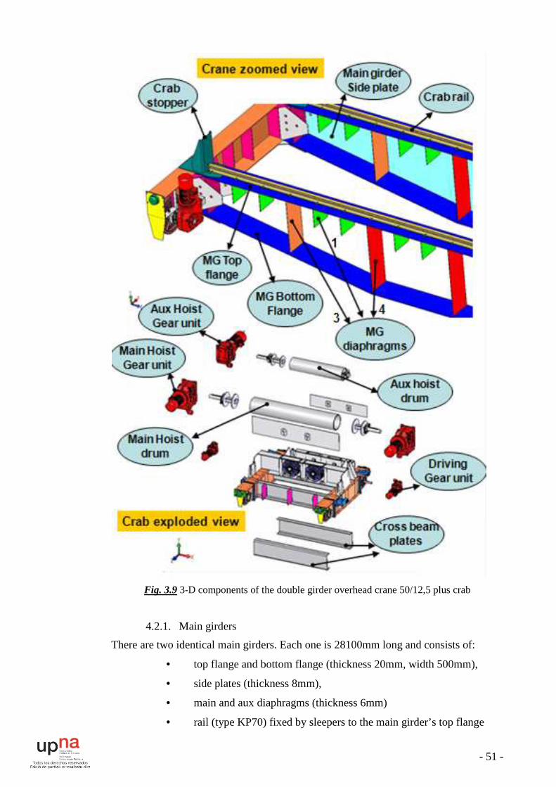
- 51 -
Fig. 3.9 3-D components of the double girder overhead crane 50/12,5 plus crab
4.2.1. Main girders
There are two identical main girders. Each one is 28100mm long and consists of:
• top flange and bottom flange (thickness 20mm, width 500mm),
• side plates (thickness 8mm),
• main and aux diaphragms (thickness 6mm)
• rail (type KP70) fixed by sleepers to the main girder’s top flange
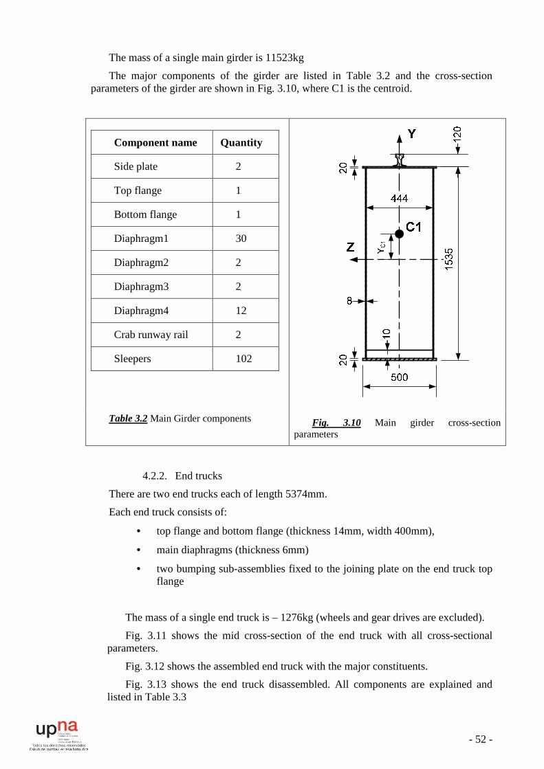
- 52 -
The mass of a single main girder is 11523kg
The major components of the girder are listed in Table 3.2 and the cross-section parameters of the girder are shown in Fig. 3.10, where C1 is the centroid.
Table 3.2 Main Girder components
Component name Quantity
Side plate 2
Top flange 1
Bottom flange 1
Diaphragm1 30
Diaphragm2 2
Diaphragm3 2
Diaphragm4 12
Crab runway rail 2
Sleepers 102
Fig. 3.10 Main girder cross-section parameters
4.2.2. End trucks
There are two end trucks each of length 5374mm.
Each end truck consists of:
• top flange and bottom flange (thickness 14mm, width 400mm),
• main diaphragms (thickness 6mm)
• two bumping sub-assemblies fixed to the joining plate on the end truck top flange
The mass of a single end truck is – 1276kg (wheels and gear drives are excluded).
Fig. 3.11 shows the mid cross-section of the end truck with all cross-sectional parameters.
Fig. 3.12 shows the assembled end truck with the major constituents.
Fig. 3.13 shows the end truck disassembled. All components are explained and listed in Table 3.3

- 53 -
Fig. 3.11 End truck cross-section parameters
Fig. 3.12 End truck (ET) assembly (side plate hidden)

- 54 -
Fig. 3.13 End truck disassembled with all components listed
End truck components (for one end truck) Comments
Number Component name Quantity
1 Side plate 2 Attachments are included
2 Top flange 1 3-D part
3 Bottom flange 1 3-D part
4 Bridge bumping set 2 subassembly
5 Crab stoppers (bumpers) 2 subassembly
6 Free wheel 1 subassembly
7 Driving wheel 1 subassembly
8 Diaphragm1 2 3-D part
9 Diaphragm2 6 3-D part
10 Driving gear motor 1 subassembly
Table 3.3 End truck components

- 55 -
4.2.3. Crane driving units
There are two crane driving units, Fig. 3.14. Each one consists of:
• gear motor (of power 11kW)
• driving wheel sub-assembly (wheel diameter 710mm) with bearings
Fig. 3.14 Crane driving unit
There have also been modeled the free crane traversing wheel sub-assemblies.
4.2.4. Rails and design tables
The crane runway rails (KP-80) and the crab runway rails (KP-70) are designed according to the standardized requirements for the dimensions, as shown in Fig. 3.15.
Fig. 3.15 Runway rail cross-section and parameters

- 56 -
Moreover, these rails are designed through the use of the design table method, available in SolidWorks.
A design table allows you to build multiple configurations of parts or assemblies by specifying parameters in an embedded Microsoft Excel worksheet [10], [11].
When you use design tables in the SolidWorks software, it is important to format the tables properly, Fig. 3.16.
Fig. 3.16 KP-70 design process with the design table
There are several different ways to insert a design table.
• to have the SolidWorks software insert a design table automatically
• to insert a blank design table
• to insert an external Microsoft Excel file as a design table
For the current case, the first way was chosen and some necessary manual corrections were done. Depending on the settings you selected, a dialog box may appear that asks which dimensions or parameters you want to add.
An embedded worksheet appears in the window, and the SolidWorks toolbars are replaced with Excel toolbars.
Cell A1 identifies the worksheet as Design Table for: <model_name>.

- 57 -
4.3. 3-D CRANE MODEL2 AND MODEL3
As mentioned in the introductory point 4.1, the carrying metal construction is the most metal-intensive part of overhead cranes. As listed in Table 3.1, the total mass of the bridge is 28173kg.
From the practice and from the literature it is well-known that positioning the main girder rails over one of the main girder side plates leads to reduction in the bridge structure mass. In this connection, the present work proposes some models of crane carrying structures designed to make the structure of the 3-D basic crane model lighter.
In these new models, the structural material is used more economically [2], [3]. Moreover, in comparison with model1, here the pressure stress in the side plate due to the crab wheels loading does not require any further increase in the side plate thickness. At the same time, neither the rails nor the top flange are subjected to considerable local bending due to the crab loading. This obviously allows for reducing the thickness of the opposing side plate as well as of the diaphragms.
However, the new models are characterized by the fact that the plane of loading does not pass through the bending center of the carrying cross-section, which produces additional main girder shear stresses. For this reason, the goal is to decrease the distance from the loading to the bending center which most commonly results in reducing the mass of the opposing side plate.
The side plate mass could be reduced by making the plate thinner and cutting extra holes through it. Therefore, two models of lighter crane structure have been designed in which the modified side plate has the same thickness but two types of holes are cut – simple holes and rimmed holes.
The following figures Fig. 3.17, Fig. 3.18 and Fig. 3.19 give the schemes of the holes positioning and dimensions
Fig. 3.20 presents the 3-D picture of the model 3 main girder design. It could be seen that the big diaphragms are also with hole which helps for further decreasing the mass of the structure.
Fig. 3.17 Main girder model2 (front view)

- 58 -
Fig. 3.18 Main girder model2 cross-section A-A parameters
Fig. 3.19 Main girder model3 cross-section parameters
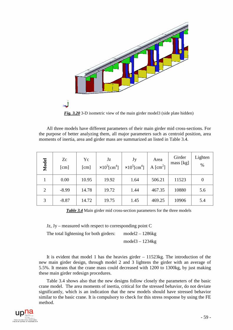
- 59 -
Fig. 3.20 3-D isometric view of the main girder model3 (side plate hidden)
All three models have different parameters of their main girder mid cross-sections. For the purpose of better analyzing them, all major parameters such as centroid position, area moments of inertia, area and girder mass are summarized an listed in Table 3.4.
Mod
el
Zc
[cm]
Yc
[cm]
Jz
×105[cm4]
Jy
×105[cm4]
Area
A [cm2]
Girder mass [kg]
Lighten
%
1 0.00 10.95 19.92 1.64 506.21 11523 0
2 -8.99 14.78 19.72 1.44 467.35 10880 5.6
3 -8.87 14.72 19.75 1.45 469.25 10906 5.4
Table 3.4 Main girder mid cross-section parameters for the three models
Jz, Jy – measured with respect to corresponding point C
The total lightening for both girders: model2 – 1286kg
model3 – 1234kg
It is evident that model 1 has the heavies girder – 11523kg. The introduction of the new main girder design, through model 2 and 3 lightens the girder with an average of 5.5%. It means that the crane mass could decreased with 1200 to 1300kg, by just making these main girder redesign procedures.
Table 3.4 shows also that the new designs follow closely the parameters of the basic crane model. The area moments of inertia, critical for the stressed behavior, do not deviate significantly, which is an indication that the new models should have stressed behavior similar to the basic crane. It is compulsory to check for this stress response by using the FE method.

- 60 -
4.3.1. Rimmed holes designing through sheet metal
Sheet metal parts are generally used as enclosures for components or to provide support to other components.
You can design a sheet metal part on its own without any references to the parts it will enclose, or you can design the part in the context of an assembly that contains the enclosed components.
Many releases ago, SolidWorks changed the way that the software dealt with sheet metal parts. In the old way, the sheet metal part was created through normal modeling features mainly centered on thin feature extrudes but also including shell features. It did not matter how you got the geometry, as long as it had a consistent thickness and the edge faces were sheared perpendicular to the material.
The new way uses a functional feature approach, which greatly simplified the feature order requirements, and at the same time added some powerful and easy-to-use feature types. This new way is what is now called the Base Flange method, and is the main tool for sheet metal creation that most sheet metal designers use today.
The basic concept with the Base Flange method is that when you insert a Base Flange feature, SolidWorks identifies that part as a sheet metal part. You can create multi-body sheet metal parts, but you can only insert one Base Flange for each part document, and so only one body can be sheet metal. If you try to create a second Base Flange feature, then SolidWorks interprets it as an attempt to add a tab, which is the alternate function of the Base Flange tool.
The sheet metal features allow the design of complex shapes and the repetitive use of configurations through the library features.
Library features are features that you create once and re-use many times. They are intended to be parametrically flexible to fit into many types of geometry, but they can also be of a fixed size and shape.
Library features reside in the Design Library. One very useful aspect of library features is that they can be driven by configurations and design tables. Once the feature is in the part, the configurations are still available, and so you can change the configuration of an applied library feature at any time.
The sheet metal forming tools (and more specifically the extruded flanges) is the method applied here for creating the rimmed holes, Fig. 3.21.
(a)
(b)
Fig. 3.21 Main girder model3 (a) rimmed hole design; (b) rimmed hole forming tool

- 61 -
Forming tools act as dies that bend, stretch, or otherwise form sheet metal to create form features such as louvers, lances, flanges, and ribs. You can insert forming tools only from the Design Library and you can apply them only to sheet metal parts. A sheet metal part has the Sheet-Metal1 feature in the FeatureManager design tree.
The presented shape is designed to create own forming tool using many of the same steps one uses to create any SolidWorks part.
The parameters of the forming tools are such that the holes to be formed on the side plate are the same as the holes in model 2. Here the new thing is the rims that are formed due to the rounded edges of the tool. The bent that remains has 36mm radius.
It is assumed that the rimmed holes could stiffen the side plate and reduce local side plate stresses. This one is to be confirmed through model analyses.

- 62 -
5. SIMULATION RESEARCH ON THE METAL STRUCTURE OF OVERHEAD BRIDGE CRANE
5.1. OVERVIEW
All the 3-D models created in the previous chapter are analyzed by the help of the finite element method (FEM).
After generating the corresponding 3-D geometry, it is transferred to the FEA (finite element analysis) application Workbench for performing the structural analyses where all necessary conditions are set for performing the investigation.
The parameters listed in Table 3.1, form the “3-D basic model” or “model1”. The basic 3-D model, after its validity is confirmed, serves as a reference point for the further investigations.
The validation is done in two ways.
• On one hand, its displacement is compared with the displacement of an ANSYS basic beam model which is in fact the widely accepted Euler-Bernoulli simply supported beam model, applied for the bridge crane.
• On the other hand, the basic 3-D model reproduces a real working crane. So the model could be validated one more time by comparing the crane static response with predefined and standardized deflection criteria (both horizontal and vertical). The deflection criteria are based on standard loading cases and predetermined values [12], [14], etc.
5.2. ANSYS BASIC BEAM MODEL
5.2.1. Overview
The ANSYS basic beam model is the first step in the validation of the 3-D basic model of the bridge crane. The bridge crane is of type double girder overhead.
If the following is assumed: no crane defects, crab center of gravity coincides with its geometric center and the payload suspension points, then both girders will have the same vertical deflection and will be subjected to the action of half the crab weight and half the load weight. So the ANSYS model is generated on the basis of a single crane girder, loaded by half the crab and half the payload weight.
5.2.2. Algorithm for generating the model
The algorithm of generating the ANSYS basic model follows closely the general FEA algorithm described in point 3.3.
The model is based on the widely accepted Euler-Bernoulli beam theory, discussed in details in point 3.4.3 of this work. The major constituents of the model are the girder, the crab and the payload - these define the geometric domain of the problem.
Next, is it required to define the element types and their properties – material and geometric.
The girder is meshed with BEAM3 finite elements, which are explained in point 3.4.4. In order to enter the required element properties (cross-sectional area, mass, area moment of inertia), an equivalent beam has been developed.
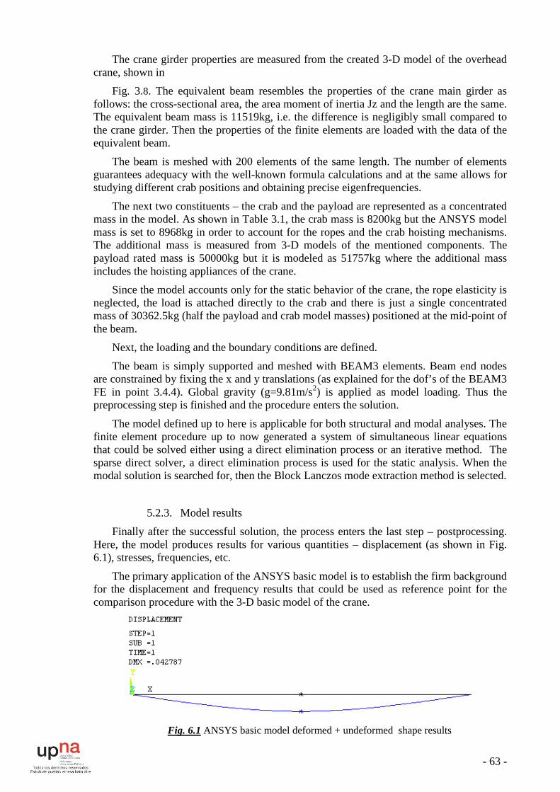
- 63 -
The crane girder properties are measured from the created 3-D model of the overhead crane, shown in
Fig. 3.8. The equivalent beam resembles the properties of the crane main girder as follows: the cross-sectional area, the area moment of inertia Jz and the length are the same. The equivalent beam mass is 11519kg, i.e. the difference is negligibly small compared to the crane girder. Then the properties of the finite elements are loaded with the data of the equivalent beam.
The beam is meshed with 200 elements of the same length. The number of elements guarantees adequacy with the well-known formula calculations and at the same allows for studying different crab positions and obtaining precise eigenfrequencies.
The next two constituents – the crab and the payload are represented as a concentrated mass in the model. As shown in Table 3.1, the crab mass is 8200kg but the ANSYS model mass is set to 8968kg in order to account for the ropes and the crab hoisting mechanisms. The additional mass is measured from 3-D models of the mentioned components. The payload rated mass is 50000kg but it is modeled as 51757kg where the additional mass includes the hoisting appliances of the crane.
Since the model accounts only for the static behavior of the crane, the rope elasticity is neglected, the load is attached directly to the crab and there is just a single concentrated mass of 30362.5kg (half the payload and crab model masses) positioned at the mid-point of the beam.
Next, the loading and the boundary conditions are defined.
The beam is simply supported and meshed with BEAM3 elements. Beam end nodes are constrained by fixing the x and y translations (as explained for the dof’s of the BEAM3 FE in point 3.4.4). Global gravity (g=9.81m/s2) is applied as model loading. Thus the preprocessing step is finished and the procedure enters the solution.
The model defined up to here is applicable for both structural and modal analyses. The finite element procedure up to now generated a system of simultaneous linear equations that could be solved either using a direct elimination process or an iterative method. The sparse direct solver, a direct elimination process is used for the static analysis. When the modal solution is searched for, then the Block Lanczos mode extraction method is selected.
5.2.3. Model results
Finally after the successful solution, the process enters the last step – postprocessing. Here, the model produces results for various quantities – displacement (as shown in Fig. 6.1), stresses, frequencies, etc.
The primary application of the ANSYS basic model is to establish the firm background for the displacement and frequency results that could be used as reference point for the comparison procedure with the 3-D basic model of the crane.
Fig. 6.1 ANSYS basic model deformed + undeformed shape results

The model reports that the max. displacement at the beam mid42.7 mm. This value is to be compared with the theoretical strength of materials formulas to verify the model validity.
5.2.4. Validation
In physics and systems theoryproperty, states that, for allcaused by two or more stimuli is the sum of the responses which would have been caused by each stimulus individu
So that if input A produces response(A + B) produces response (
Mathematically, for astimulus (input) and y is some sort of response (output), the superposition (i.e., sum) of stimuli yields a superposition of the respective responses
The differential equations for a deflected beam are linear differentitherefore the slope and deflection of a beam are linearly proportional to the applied loads Therefore, the slope and deflection of a beam due to several loads is equal to the sum of those due to the individual loads. In other words, the indisuperimposed to determined a combined response, hence the method of superposition.
This is a very powerful and convenient method since solutions for many support and loading conditions are readily available in various engineerinprinciple of superposition, we may combine these solutions to obtain a solution for more complicated loading conditions
The deflection equation of the complex beam is the addition of the two simpler beam equations, or more:
In the case of deflection of beams, the priholds for the material and if the deflection and rotation of the beam are small.
The method of superposition is most useful when the loading system obe subdivided into loading conditions that produce deflections that are already known.
In this case we are going to apply the
formulas for the case of concentrated load
The model reports that the max. displacement at the beam mid-This value is to be compared with the theoretical strength of materials formulas
rify the model validity.
Validation
systems theory, the superposition principle, also known for all linear systems, the net response at a given place and time
caused by two or more stimuli is the sum of the responses which would have been caused by each stimulus individually.
produces response X and input B produces response) produces response (X + Y).
Mathematically, for a linear system, F, defined by F(x) = y, whereis some sort of response (output), the superposition (i.e., sum) of
stimuli yields a superposition of the respective responses:
1 2 1 2( ....) ( ) ( ) ...F x x F x F x+ + = + +
The differential equations for a deflected beam are linear differentitherefore the slope and deflection of a beam are linearly proportional to the applied loads Therefore, the slope and deflection of a beam due to several loads is equal to the sum of those due to the individual loads. In other words, the individual results may be superimposed to determined a combined response, hence the method of superposition.
This is a very powerful and convenient method since solutions for many support and loading conditions are readily available in various engineering handbooks. Using the principle of superposition, we may combine these solutions to obtain a solution for more complicated loading conditions
The deflection equation of the complex beam is the addition of the two simpler beam
δ(x) = δ1(x) + δ2(x)+……
of deflection of beams, the principle of superposition is valid if Hooke’s law holds for the material and if the deflection and rotation of the beam are small.
The method of superposition is most useful when the loading system obe subdivided into loading conditions that produce deflections that are already known.
In this case we are going to apply the superposition principle to our simple beam, the
of concentrated load (P) and uniformed load (ω
2 21( ) (3 4 )
48
P xy x l x
E I
⋅= ⋅ − ⋅⋅ ⋅
- 64 -
-point and the value is This value is to be compared with the theoretical strength of materials formulas
, also known as superposition , the net response at a given place and time
caused by two or more stimuli is the sum of the responses which would have been caused
produces response Y then input
, where x is some sort of is some sort of response (output), the superposition (i.e., sum) of
( ....) ( ) ( ) ...
The differential equations for a deflected beam are linear differential equations, therefore the slope and deflection of a beam are linearly proportional to the applied loads Therefore, the slope and deflection of a beam due to several loads is equal to the sum of
vidual results may be superimposed to determined a combined response, hence the method of superposition.
This is a very powerful and convenient method since solutions for many support and g handbooks. Using the
principle of superposition, we may combine these solutions to obtain a solution for more
The deflection equation of the complex beam is the addition of the two simpler beam
nciple of superposition is valid if Hooke’s law holds for the material and if the deflection and rotation of the beam are small.
The method of superposition is most useful when the loading system on the beam can be subdivided into loading conditions that produce deflections that are already known.
to our simple beam, the
ω) are as follows [21]:

Once made, the separate calculations are then summed up to obtain the value of the displacement that is later compared with the value reported by ANSYS.
Calculations are done in the Excel environment. The table below shows the displacement results for an array of points located on the beam at a step of 0.5m. The maximum reported displacement is in the middle of the beam, at 14.05m.
x (m)
00.51
1.52
2.53
3.54
4.55
5.56
6.57
7.58
8.59
9.510
10.511
11.512
12.513
13.514
14.05
3 2 3
2( ) ( 2 )24
xy x l l x x
E I
ω ⋅= − ⋅ ⋅ +⋅ ⋅
Once made, the separate calculations are then summed up to obtain the value of the displacement that is later compared with the value reported by ANSYS.
done in the Excel environment. The table below shows the displacement results for an array of points located on the beam at a step of 0.5m. The maximum reported displacement is in the middle of the beam, at 14.05m.
P ω P+ωx (m) y1 (mm) y2 (mm) y (mm)
0 0.0 0.0 0.0 0.5 1.85 0.47 2.311 3.69 0.93 4.62
1.5 5.52 1.39 6.922 7.34 1.85 9.20
2.5 9.15 2.30 11.453 10.92 2.74 13.67
3.5 12.67 3.18 15.854 14.39 3.60 17.99
4.5 16.07 4.01 20.085 17.70 4.41 22.11
5.5 19.30 4.79 24.086 20.83 5.15 25.99
6.5 22.32 5.50 27.827 23.74 5.83 29.57
7.5 25.09 6.15 31.248 26.38 6.44 32.82
8.5 27.59 6.71 34.309 28.72 6.97 35.69
9.5 29.77 7.20 36.9610 30.73 7.40 38.13
10.5 31.59 7.59 39.1811 32.36 7.75 40.11
11.5 33.02 7.89 40.9112 33.58 8.00 41.58
12.5 34.02 8.09 42.1113 34.35 8.16 42.50
13.5 34.55 8.20 42.7514 34.63 8.21 42.84
14.05 34.63 8.21 42.84
- 65 -
( ) ( 2 )
Once made, the separate calculations are then summed up to obtain the value of the displacement that is later compared with the value reported by ANSYS.
done in the Excel environment. The table below shows the displacement results for an array of points located on the beam at a step of 0.5m. The maximum reported displacement is in the middle of the beam, at 14.05m.
ω y (mm)
1 2 2 0 5 7 5
7.99 08 1
08 5.99
2 57 4 2 0
69 6.96
3 18 1 1 8 1 0 5 4 4

- 66 -
The maximum displacement is equal to 42.84 mm and with ANSYS the value at the beam mid-point is 42.79 mm, therefore the error is less than 1%.
As show before this insignificant error confirm us that we can trust in the results of ANSYS for the basic beam model and also verify the model validity.
As mentioned, the ANSYS basic model could provide results for the natural frequencies of the system. For this purpose, the model is set to a modal analysis option and the first 6 frequencies are requested. A frequency value of interest for the current study is the f1=2.461Hz value that corresponds to the first vertical modal shape of the beam (along y-axis). The model also provides results for the higher modes: f2=24.55Hz and f3=39.96Hz, as shown in Fig. 6.2 cases (a), (b) and (c).
(a)
(b)
(c)
Fig. 6.2 ANSYS basic model – the first three vertical modal shapes,
deformed + undeformed shape results
This concludes the discussion about the ANSYS basic model and the study forwards to the generation of the 3-D basic model.

- 67 -
5.3. 3-D BASIC MODEL SIMULATION RESEARCH.
5.3.1. Preparing the 3-D basic model simulation.
The 3-D basic model of the crane is analyzed with the help of the ANSYS Workbench FEA application. The ANSYS Workbench FEA provides a unified working environment for developing and managing a variety of CAE information and makes it easier for setting up and work with data at a high level. The crane geometry generated in SolidWorks is imported here, where various boundary conditions, loadings and mesh controls provide powerful environment for the analyses.
The 3-D crane geometry is to be meshed with 3-D elements (solid elements) and such models are the hardest to prepare, the most tedious to check for errors, and the most demanding of computer resources. However, when properly meshed and the proper boundary conditions, loadings and material properties are set, then the model could reveal in full details even the most complex stressed behavior of the structure.
The imported geometry includes numerous of parts, many of them are contacting each other or have complex geometry which requires that special care be taken of the mesh. The number of finite elements in the mesh will directly influence the reasonable solution time. Solution accuracy usually asks for mesh refinement but PC resources impose limit on the FE number. The decreased number of elements, however, should not sacrifice the solution accuracy.
So, after the geometry is imported, detailed attention is paid to the mesh by placing proper mesh controls on the crane components. The meshing procedure is iterative, i.e. several meshes were obtained and solved for after the final mesh appearance,
Fig. 6.3 is obtained.
Fig. 6.3 3-D basic model final mesh (some main girder and end truck plates are hidden)

- 68 -
The mesh consists of 38962 finite elements and 72937 nodes. The major element types used are:
• 10-Node Quadratic Tetrahedron Solid187- 10-Node Tetrahedral Structural Solid
• 20-Node Quadratic Hexahedron Solid186 - 20-Node Hexahedral Structural Solid
• 20-Node Quadratic Wedge Solid186 - 20-Node Hexahedral Structural Solid
• Quadratic Quadrilateral Contact Conta174 - Hi-order Surface to Surface Contact
• Quadratic Quadrilateral Target Targe170 - Surface Contact Target;
• Quadratic Triangular Contact Conta174 - Hi-order Surface to Surface Contact
Detailed description of the SOLID186 and SOLID187 characteristics is given in point 3.4.6.
The material used is for the bridge structure is steel with properties:
Elastic modulus 112 10E Pa= ×
Poisson’s ratio 0.3ν =
Density 37850 /kg m
Tensile yield strength 250MPa
Tensile ultimate strength 460MPa
The crab is not part of the current investigation objective. Additionally, if it is left in the 3-D model as is, Fig. 6.4, then there is a high possibility of not being able to achieve reasonable solution times and mesh. That is why the crab is greatly simplified, Fig. 6.5.
Fig. 6.4 Detailed 3-D geometry of the crab

- 69 -
Fig. 6.5 Simplified crab geometry
Fig. 6.6 Scheme of the simplified crab
The simplified crab geometry from top view, Fig. 6.6, is a rectangle with dimensions 3000x3400mm. Lines L1 and L3 pass through the middle of the wheels. Lines L2 and L4 pass through the center of the wheels.

- 70 -
Distance L2 to L4 is 2500 (as in the original crab).
Distance L1 to L3 is 2850 (as in the original crab) which is the same distance between center lines of the crane main girders.
Fig. 6.6 also shows the geometric center (GMC) of the crab and the first local coordinate system OXYZ (LocalCS1).
It is assumed that the simplified geometry is non-deforming and has no mass. So, the crab mass M1 is concentrated entirely in its center of mass (CM) and the CM position must be known. The CM position is measured from the real crab, with respect to Coordinate system 1, Fig. 6.4. Coordinate system 1 (CS1) origin is in the plane where the crab wheels are in contact with the main girder rail, and CS1 origin is at equal distances from the crab wheels.
The Y-value of the CM (measured from CS1) determines the thickness of the crab measured from the wheel contact with the rail. The top face of the block, Fig. 6.5 will be the plane where the CM will be located. For additional positioning of the CM, the local coordinate system OXYZ, Fig. 6.6, is created and its origin is on the vertex of the rectangle as shown.
The payload mass M2 is also assumed as a concentrated mass. It is located on the bottom face of the block. A second local coordinate system OXYZ (LocalCS2) is located on this bottom face. The M2 position in the 3-D model is with respect to LocalCS2. The payload is assumed to be suspended from the main drum on a 5m rope. So these determine the location of the M2 in the 3-D model.
So briefly there is the first concentrated mass M1=8968kg and the second concentrated mass M2=51757kg and the mass values are explained in the ANSYS basic model. In the way the crab and payload masses are defined makes the 3-D model quite flexible. Masses could be easily changed and relocated.
Next is the pre-processing stage where the load boundary conditions are to be assigned. There are boundary conditions defined for all of the four crane wheels. Boundary conditions fix the crane wheels vertical displacement (along Y-axis, Fig. 6.3). In order to account for the masses, a global system gravity is introduced as g=9.81m/s2 along the Y-axis.
5.3.2. 3-D basic model simulation results.
The introduced loadings and contacts of type bonded turned the problem to linear static structural solution and a direct solver is used. The solution took about 30-40mins and after a successful solution, there could be retrieved a multitude of results for the crane static structural response as shown in Fig. 6.7, Fig. 6.8.

- 71 -
Fig. 6.7 Equivalent (von-Mises) stresses in the bridge structure
(crab and side plate of the far girder are hidden; stress values are measured at certain points)
Fig. 6.8 Vertical (Y-axis) deformation of the crane
(deformation values are measured at certain points)

- 72 -
The model allows us to measure at points and cross-sections that are inaccessible to the real gauging experiments, Fig. 6.9.
Fig. 6.9 Equivalent stresses measured at points on the diaphragms, inner walls of side plates and main girder mid cross-section (some side plates and diaphragms are hidden)
Results are also provided and could be measured at various crane components, such as the end trucks Fig. 6.10, the wheels, etc.

- 73 -
Fig. 6.10 Equivalent stresses measured at points on the end truck and near the driving crane
wheel (main girders are hidden)
As mentioned, the 3-D model is quite flexible. Besides the static structural results it could provide values of the crane frequency response, as shown in figures Fig. 6.11 and Fig. 6.12.
Fig. 6.11 First vertical (Y-axis) modal shape of the crane
(first vertical natural frequency f1=2.44Hz)

- 74 -
Fig. 6.12 Modal shape 6 of the crane (natural frequency 4.18Hz)
The 3-D modal analysis as compared to the ANSYS basic beam modal analysis offers much more detailed response picture. As shown in Fig. 6.12, here all possible shapes and frequencies could be derived and analyzed.
5.3.3. 3-D basic model vs ANSYS basic model.
After the 3-D basic model is solved and results acquired, it is necessary to compare these values with the ones from the ANSYS basic beam model. This was mentioned as one of the steps for the 3-D model validation.
Parameter ANSYS basic beam
model 3-D basic model Error ∆%
Main girder vertical displacement [mm]
42.7 43.3 1.41
First natural vertical frequency f1 [Hz]
2.46 2.44 0.82
Table 6.1 Comparison of the 3-D basic model with the ANSYS basic beam model

- 75 -
Table 6.1 clearly confirms that the 3-D basic model conforms to the theoretical considerations. The model is properly conditioned – the supports are well established, and the mesh is well designed.
The max. displacement of the 3-D basic model compared to the ANSYS basic beam model max. displacement leads to an acceptable error of not more than 1.5%.
Moreover, the natural frequency is included as a very significant comparison parameter, when comparing the Euler-Bernoulli simply supported ANSYS beam model with the 3-D basic model.
It is obvious that the first vertical natural frequency of the 3-D crane is less than 1% compared to the ANSYS model, take into account that the frequency to be compared must be the first vertical one because with the ANSYS basic model only the vertical displacement could be check.
The natural frequencies are quite important especially for performing dynamic studies of the structure [19].
Finally, the 3-D basic model is validated with respect to theory.
5.3.4. 3-D basic model static structural analyses.
There are lots of forces acting on the crane structure – crab and crane deadweight, payload, inertia forces, etc. In order to account for all of them in a fashion that is close enough to the real operating conditions, these forces could be grouped into several loading cases.
• Loading case 1 – Accounts for the live load vertical deflection of the structure. Includes crab and bridge weights plus the rated load. Used to define the endangered stress points on the metal structure.
• Loading case 2 – Deflection criteria (horizontal) – used to estimate the max horizontal deflection and compare it to the max permissible horizontal deflection allowed for bridge cranes. Both vertical and horizontal loadings are included with the latter due to sudden starts or stops of the crane with hoisted payload.
• Loading case 3 – Crane testing requirement with 125% of rated load capacity. It serves as a check for the vertical dynamic forces and safety considerations of the structure. Includes the vertical loadings due to sudden lifting or lowering of the payload when the crane is immovable.
• Loading case 4 – Deflection criteria (vertical) – used to estimate the max vertical deflection and compare it to the max permissible vertical deflection allowed which for bridge cranes is L/700 (L is the bridge span).

- 76 -
Loading case 1
This case loads the model in the plain of main girder symmetry as shown in Fig. 6.13.
Fig. 6.13 Loading scheme
Designations are:
[ ]/ N/mmq G L= - intensity of the uniformly distributed load from the main girder
deadweight;
[ ] NmG - main girder weight;
2,5mb= - crab wheel-gauge;
28,5mL = - crane span;
F1 and F2 – compression on crab wheels;
C-C – main girder mid cross-section;
C1-C1 – main girder cross-section under the crab wheel 1 625 mma = ;
C2-C2 – main girder cross-section at distance 2 8755 mma = from the girder left
end;
D-D – cross section near the end of the girder 3 590 mma = ;
For 1 / 4a b= crab wheels compression gets the form:
( )1 21
4 cbF F F G Qψ= = = + (2.45)
where, cbG - crab weight, ( )vQfψ = - dynamic coefficient as a function of the
payload speed; v 2,4m/minQ = - payload speed
The vertical loading, due to gravity, is:
crab weight cbG ;
payload weight 500 kNQ= ;
main girder weight 115,39 kNMGG =

- 77 -
Main girders and end trucks geometric parameters are shown in Fig. 3.10 and Fig. 3.11.
The normal σX and the equivalent σEq stresses are measured at points around cross-sections C-C, C1-C1, C2-C2 and the supporting D-D sections as given in Fig. 6.13, Fig. 6.14 and Fig. 6.15, for crab positioned in the bridge midst.
Fig. 6.14 Designations of girder locations and components
In model1 for sections C-C, C1-C1 and C2-C2, flange points are located at a step of 100mm and on side plates points are at 300mm step. For models 2 and 3, the flange points are located at a step of 124mm, on side plates the step is equal to model1.
Fig. 6.15 Points on sections C-C, C1-C1, C2-C2 and D-D for the girder near the drive

- 78 -
For section D-D the step is 160mm for the side plates.
Measured are also the natural frequencies and the static deformation of the crane structure.
The measurements also include the equivalent stresses at points on characteristic main girder section as shown in Fig. 6.16.
Fig. 6.16 Characteristic end truck points
The model allows to gather data for the equivalent stresses Eqσ , normal stresses
( Xσ , Yσ , Zσ ), shear stresses (XYτ , YZτ , XZτ ), directional deformations ( XU , YU ,
ZU ) etc. Some of the measured data are summarized in several tables and graphs below.
The cross-sectional values pertain to the main girder near the drive. This girder is chosen since the crab CM is displaced and the higher crab reactions are located namely on the girder near the drive.
Location Parameter
Point
0 1 2 3 4 5
Top
flan
ge
[ ] Eq MPaσ 44.37 42.33 40.54 40.5 42.14 43.95
[ ] X MPaσ
-37.6 -37.3 -38.17 -38.57 -26.71 -39.18
[ ] XY MPaτ
0.35 -0.46 -1.28 -1.25 0.37 0.52
[ ] YU mm
-43.9 -43.8 -43.7 -43.7 -43.7 -43.7
[ ] ZU mm
-0.012 -0.023 -0.032 -0.041 -0.05 -0.06

- 79 -
Bot
tom
flan
ge
[ ] Eq MPaσ 94.67 94.3 93.93 93.85 94.05 94.26
[ ] X MPaσ
94.23 94.18 94.17 94.19 94.41 94.63
[ ] XY MPaτ
-8.7×10⁻³
-0.03 2.5×10⁻³ 3.7×10⁻³ -7×10⁻⁴ -4.8×10⁻³
[ ] YU mm
-43.9 -43.8 -43.8 -43.7 -43.7 -43.7
[ ] ZU mm
-0.73 -0.72 -0.70 -0.69 -0.68 -0.66
Out
er s
ide
plat
e
[ ] Eq MPaσ 40.18 16.94 17.16 43.7 75.52 92.97
[ ] X MPaσ
-41.95 -17.5 8.6 36.35 64.73 92.84
[ ] XY MPaτ
-4.04 0.5 3.78 5.1 4.9 0.36
[ ] YU mm
-43.7 -43.8 -43.9 -43.9 -43.8 -43.7
[ ] ZU mm
-0.05 -0.15 -0.28 -0.41 -0.53 -0.66
Inne
r si
de p
late
[ ] Eq MPaσ 43.1 16.25 16.49 43.58 75.16 92.64
[ ] X MPaσ
-45.05 -17.59 9.04 36.53 64.8 91.05
[ ] XY MPaτ
-0.5 0.29 3.76 5.2 5.1 4.2
[ ] YU mm
-43.9 -43.8 -43.9 -43.9 -43.8 -43.9
[ ] ZU mm
-0.04 -0.2 -0.32 -0.45 -0.58 -0.73
Table 6.2 Values for cross-section C-C
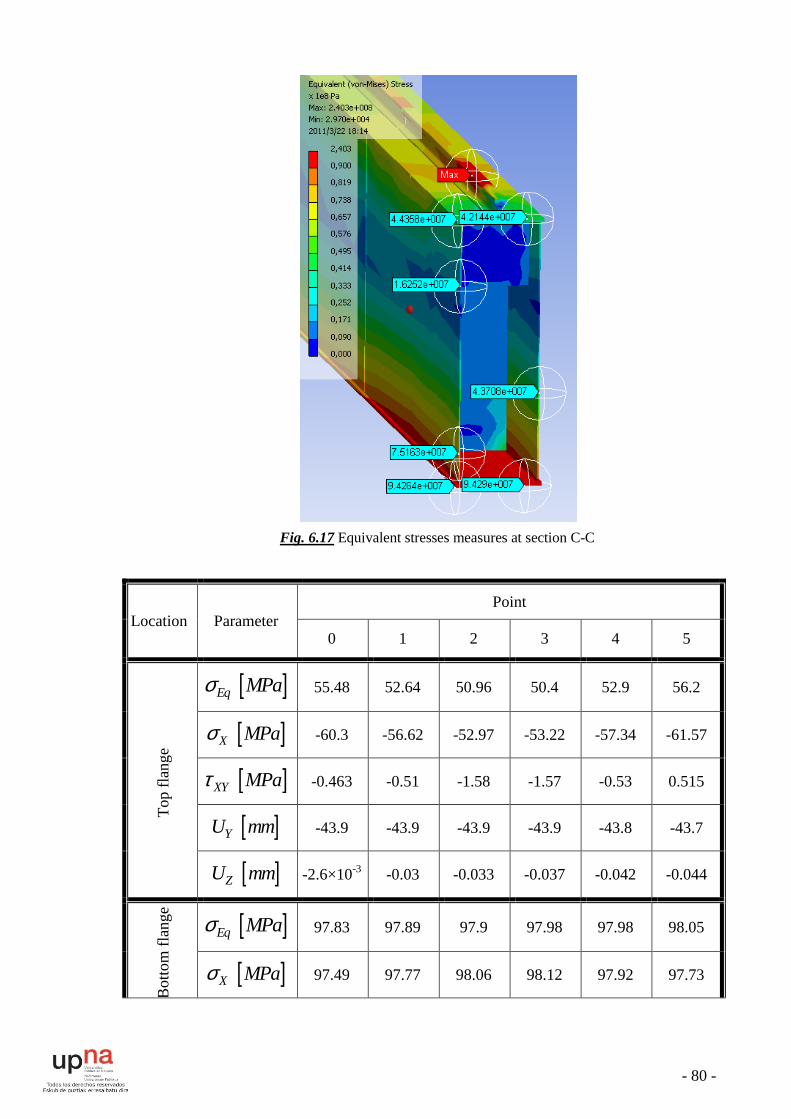
- 80 -
Fig. 6.17 Equivalent stresses measures at section C-C
Location Parameter Point
0 1 2 3 4 5
Top
flan
ge
[ ] Eq MPaσ 55.48 52.64 50.96 50.4 52.9 56.2
[ ] X MPaσ
-60.3 -56.62 -52.97 -53.22 -57.34 -61.57
[ ] XY MPaτ
-0.463 -0.51 -1.58 -1.57 -0.53 0.515
[ ] YU mm
-43.9 -43.9 -43.9 -43.9 -43.8 -43.7
[ ] ZU mm
-2.6×10⁻³ -0.03 -0.033 -0.037 -0.042 -0.044
Bot
tom
flan
ge
[ ] Eq MPaσ 97.83 97.89 97.9 97.98 97.98 98.05
[ ] X MPaσ
97.49 97.77 98.06 98.12 97.92 97.73

- 81 -
[ ] XY MPaτ
0.098 0.045 -4.2×10⁻³ -0.063 0.039 0.1
[ ] YU mm
-43.87 -43.82 -43.78 -43.74 -43.7 -43.66
[ ] ZU mm
-0.74 -0.72 -0.71 -0.69 -0.67 -0.63
Out
er s
ide
plat
e
[ ] Eq MPaσ 52.8 24.73 15.51 36.76 66.25 95.98
[ ] X MPaσ
-51.62 -24.37 4.297 34.38 64.69 96.49
[ ] XY MPaτ
-2.92 1.58 4.96 4.95 5.06 0.55
[ ] YU mm
-43.7 -43.7 -43.7 -43.7 -43.7 -43.6
[ ] ZU mm
-0.073 -0.19 -0.3 -0.43 -0.56 -0.66
Inne
r si
de p
late
[ ] Eq MPaσ 54.77 24.57 15.92 36.86 65.43 96.16
[ ] X MPaσ
-52.77 -24.96 3.887 33.88 64.35 96.32
[ ] XY MPaτ
-2.83 1.83 5.38 5.34 5.38 5.47
[ ] YU mm
-43.9 -43.9 -43.9 -43.9 -43.9 -43.8
[ ] ZU mm
-0.015 -0.15 -0.29 -0.43 -0.56 -0.72
Table 6.3 Values for cross-section C1-C1

- 82 -
Fig. 6.18 Horizontal (Z-axis) deformation in section C1-C1
Location Parameter Point
0 1 2 3 4 5
Top
flan
ge
[ ] Eq MPaσ 55.05 55 54.73 54.75 54.87 54.83
[ ] X MPaσ
-56.05 -55.8 -55.53 -55.47 -55.67 -55.85
[ ] XY MPaτ
-0.57 -7.23 -7.71 -7.54 -6.42 -4.77
[ ] YU mm
-36.72 -36.7 -36.6 -36.59 -36.54 -36.5
[ ] ZU mm
0.023 0.015 7.7×10⁻³ 7×10⁻⁵ -7.6×10⁻³ -0.015
Bot
tom
flan
ge
[ ] Eq MPaσ 73.15 73.34 73.51 73.57 73.46 73.38
[ ] X MPaσ
73.07 73.35 73.63 73.67 73.5 73.3
[ ] XY MPaτ
-0.36 -0.086 0.17 0.155 -0.123 -0.43
[ ] YU mm
-36.7 -36.65 -36.61 -36.56 -36.52 -36.47
[ ] ZU mm
-0.71 -0.69 -0.68 -0.67 -0.66 -0.65
Out
er
side
pla
te
[ ] Eq MPaσ 53.91 31.4 17.18 26.28 48.25 71.9
[ ] X MPaσ
-53.92 -28.91 -3.74 21.76 46.14 71.66

- 83 -
[ ] XY MPaτ
0.344 -0.78 -0.195 -0.196 -0.804 0.281
[ ] YU mm
-36.51 -36.52 -36.53 -36.53 -36.51 -36.48
[ ] ZU mm
-0.24 -0.13 -0.27 -0.41 -0.53 -0.64 In
ner
side
pla
te [ ] Eq MPaσ 54.06 31.65 16.92 25.68 47.96 72.3
[ ] X MPaσ
-54.02 -29.33 -4.1 21.4 46.6 71.77
[ ] XY MPaτ
-0.56 -6.97 -7.48 -7.3 -6.2 -4.58
[ ] YU mm
-36.71 -36.73 -36.73 -36.73 -36.72 -36.7
[ ] ZU mm
0.14 -0.14 -0.27 -0.39 -0.54 -0.69
Table 6.4 Values for cross-section C2-C2
Fig. 6.19 Equivalent stresses at section C2-C2

- 84 -
Location Parameter Point
0 1 2 3 4 5
Top
flan
ge
[ ] Eq MPaσ 5.578 8.38 9.38 9.57 9.26 6.44
[ ] X MPaσ
-1.94 -5.8 -8.5 -8.84 -6.67 -3.22
[ ] XY MPaτ
-0.54 -0.042 0.29 0.32 -0.023 -0.55
[ ] YU mm
-4.54 -4.49 -4.45 -4.4 -4.38 -4.3
[ ] ZU mm
0.17 0.17 0.17 0.17 0.17 0.17
Bot
tom
flan
ge
[ ] Eq MPaσ 17.51 19.58 19.42 19.87 19.91 19.8
[ ] X MPaσ
17.55 19.54 20.71 21.31 20.86 20.18
[ ] XY MPaτ
-3.32 -3.62 -3.83 -3.92 -3.85 -3.76
[ ] YU mm
-4.55 -4.52 -4.48 -4.43 -4.37 -4.31
[ ] ZU mm
-0.27 -0.27 -0.27 -0.27 -0.27 -0.27
Out
er s
ide
plat
e [ ] Eq MPaσ 20.2 18.7 17.95 20.13 19.97 16.56
[ ] X MPaσ
-9.2 -7 -4.1 6.35 8.05 8.8
[ ] XY MPaτ
-10.3 -10.1 -10.12 -10.1 -10.8 -3.87
[ ] YU mm
-4.31 -4.31 -4.31 -4.31 -4.32 -4.32
[ ] ZU mm
0.16 0.1 5.3×10⁻³ -0.12 -0.21 -0.25
Inne
r si
de p
late
[ ] Eq MPaσ 19.21 18.24 17.81 19.71 19.46 15.1
[ ] X MPaσ
-6.3 -6.02 -4.04 6.1 7.31 7.9
[ ] XY MPaτ
-2.3 -9.9 -10 -10.7 -10.7 -3.54
[ ] YU mm
-4.53 -4.53 -4.53 -4.54 -4.54 -4.54
[ ] ZU mm
0.17 0.08 -6.4×10⁻³ -0.07 -0.17 -0.26
Table 6.5 Values for cross-section D-D

- 85 -
Fig. 6.21 Variation of the equivalent stresses in the different points of bottom flange along the characteristic sections of the beam
As shown in Fig. 5.21, stresses at different bottom flange points remain almost unchanged for the corresponding section. However, the stress values at the same point in the different sections tend to vary as shown in Fig.5.22.
The reported stress in the middle cross section is high (94.67MPa) and this value is even higher in section C1-C1, reaching up to 97.73 MPa. Comparison among the max stress values of all the sections yielded that the critical section is under the crab wheel. This conforms directly to the theory that the maximum bending moment appears at a distance of 1/4 of the crab span from the middle of the bridge.
0
10
20
30
40
50
60
70
80
90
100
110
0 1 2 3 4 5
C-C
C1-C1
C2-C2
D-D
Section
MPa
Point
Fig. 6.20 Equivalent stresses at section D-D

- 86 -
From this critical point, the stress values go down to 17.51MPa in the section near the end truck, which again conforms to the strength of materials postulates.
Fig. 6.22 Equivalent stresses at point 0 of bottom flange
Parameter Point
W F E E1
[ ] Eq MPaσ 17.45 51.6 48.76 80.7
[ ] X MPaσ
3.88 0.45 -44.4 58
[ ] Y MPaσ
-1.43 15.3 -5.05 76.2
[ ] Z MPaσ
-13.5 15.9 -12 41.06
[ ] XY MPaτ
-0.45 -1.68 0.102 1.39
[ ] YZ MPaτ
-6.64 28.3 0.49 -9.9
[ ] XZ MPaτ
-0.3 -0.6 -19.8 41.1
[ ] XU mm
2.93 -0.43 2.89 -0.96
[ ] YU mm
-0.64 -0.8 -1.76 -1.77
[ ] ZU mm
-0.18 0.16 -0.16 0.14
Table 6.6 End truck characteristic points
94,67
97,73
73,15
17,51
10
20
30
40
50
60
70
80
90
100
110
C-C C1-C1 C2-C2 D-D
MPa

- 87 -
Fig. 6.23 Horizontal (Z-axis) deformation in end truck
Loading case 2
It is used to estimate the max horizontal deflection and compare it to the max permissible horizontal deflection allowed for bridge cranes. Both vertical and horizontal loadings are included with the latter due to sudden starts or stops of the crane with hoisted payload. The loading follows the scheme in Fig. 6.24.
Fig. 6.24 Second loading scheme
- 88 -
Designations are:
[ ]1 2, Nin inF F - horizontal inertia forces due to the vertical forces F1 and F2;
[ ]. / N/mmq G Lϕ= - intensity of the uniformly distributed load from the main
girder deadweight;
( )vfϕ = - dynamic amplification factor due to crane motion;
( 1ϕ = for v 60m/min< and 1ϕ > for v>60m/min);
[ ]in . / . N/mmq aG L g= - intensity of the uniformly distributed force from the main
girder mass;
2 m/sa - crane acceleration/deceleration
29,81 m/sg = - gravity
The stressed state is evaluated by the normal stress σX in the central section C-C. The stress is defined by the known relation:
in inF q
V H HZ
Y Z
M M M
W Wσ += ± (2.46)
, ,in inF qV H HM M M are respectively the moment due to vertical forces, the moment due
to the horizontal concentrated forces and the moment due to the horizontal uniformly distributed inertia forces.
,Y ZW W are resistive moments in both planes of the vertical section of the main girder.
Investigations are carried for crab position in the bridge midst.
The horizontal loading is applied as a horizontal acceleration 20.5 /a m s= according
to [20]. The acceleration is applied opposite to z-axis,
Fig. 6.3.
In real-world situations, the payload suspended from the crab is also subjected to this acceleration and as a consequence the payload swings.
The max angle of rope swing from its vertical position is given as
max2a
gα = − (2.47)
There is a range of values for the acceleration a :
• 20.1 0.2 /a m s= ÷ - acceleration of cranes handling molten metal
• 20.3 0.4 /a m s= ÷ - acceleration of cranes in normal operation when
crane speed are 80m/min to 120m/min (1.33m/s to 2m/s);

- 89 -
• 20.5 /a m s= - acceleration for the majority of cranes
• 20.6 /a m s= - acceleration of cranes in extreme modes of condition
(sudden stops)
• 21 1.2 /a m s= ÷ - acceleration of grabbing cranes
The currently investigated crane is a general purpose crane and it is suitable to assume that the acceleration is a = 0.5m/s2
Then the max angle is max
2 0.50.102 5 50' 6deg
gα ×= = ≈ ≈�
For cranes with capacities up to 50 tonnes, the height of suspension cannot be less than 4 to 5 meters.
It is selected that the height of suspension, i.e. the rope length, be 5meters.
A 5meter rope that swings 6deg from vertical is a clear sign that the payload Z-coordinate changes
The Z-coordinate changes and is calculated ( )5meters sin 6 deg 0.523m× =
Since the rope swings to the positive direction of the z-axis of the model, it follows, that the payload point position changes and is z= 1700+523≈2.23m
This new coordinate is entered and the concentrated mass M2 is easily relocated.
Two of the crane supports have their z-translations fixed so as to account for the fact that the crane has stopped suddenly which caused the acceleration.
Again lots of values could be measured. The ones that are of major interest are summarized in the table below:
Parameter Value
[ ] MaxEq MPaσ 110.65
[ ] MaxX MPaσ
110.7
[ ]max YU mm
-46.78
[ ]max ZU mm
10.1
Table 6.7 Max. values for section C-C

- 90 -
According to the rigidity requirements, point 1.6.2, the horizontal deflection,
[ ]ZU mm , is the maximum deflection ratio allowed for a bridge crane or runway. This
value is L/600, where L is the span of a bridge crane.
For this case, the bridge span is L=28500mm, then L/600=47.5mm.
As shown in Table 6.7, the max deflection [ ]maxZU mm is below the 47.5mm value
and it follows that the crane conforms to this rigidity requirement, with a safety factor higher than 4.
Fig. 6.25 shows top view of the crane horizontal deflection.
Fig. 6.25 Crane horizontal deflection for loading case 2
Loading case 3
Crane testing requirement with 125% of rated load capacity. It serves as a check for the vertical dynamic forces and safety considerations of the structure. Includes the vertical loadings due to sudden lifting or lowering of the payload when the crane is immovable.
The rate payload is 50000kg and with 125% of rated load capacity yields 50000*1.25=62500kg
The hoisting appliances, described in point 5.2.2, sum up to 1757kg, so the final mass M2 is 62500+1757=64257kg
This crane test load is typically specified by both [13] and [14] for safety purposes and dynamic loadings.
The max vertical girder deflection is max 51.4YU mm= −
Fig. 6.26 shows isometric view of the crane vertical deflection.
The max equivalent stress of the girder is max 282.5Eq MPaσ =
.

- 91 -
The values are again a proof of the fact that the crane can withstand the dynamic overload with 125%. However the max equivalent stress is higher than the tensile yield strength this plastically deformed specimen will not return to its original size and shape when unloaded. Note that there will be elastic recovery of a portion of the deformation. For many applications, plastic deformation is unacceptable, and is used as the design limitation.
At any rate, the max stress is underneath the tensile ultimate strength with with a overmeasure of over 60%.
Fig. 6.26 Crane vertical deflection for loading case 3
Loading case 4
It is used as the deflection criteria (vertical) – estimates the max vertical deflection and compares it to the max permissible vertical deflection allowed which for bridge cranes is L/700 (L is the bridge span).
The mass of the crane, the crab, the hoisting appliances and the ropes are all neglected. Only the payload mass of 50ton is assumed so as to compare the crane vertical deflection to a specified standard deflection.
For this crane L/700=28500/700=40.72mm
The max vertical deflection for this case is max 28.98YU mm= −
It is evident that the crane is properly constructed and conforms to the vertical deflection criteria.

- 92 -
5.4. 3-D MODELS – MODEL2 AND MODEL3 STRUCTURAL ANALYSES
5.4.1. Review
These two models aim at decreasing the mass of the crane structure but at the same time keeping the same stressed state of the 3-D basic crane. Detailed description of the modeling procedure, major dimensions and relations is given in point 4.3.
Here the two models are tested using the same loading cases 1, 2, 3 and 4 and the results obtained are gathered, analyzed and compared with the basic crane response. Due to the large amount of data processed, the tables, graphs and figures that follow summarize briefly some of the more important, for comparison purposes, information.
Again the measured points of the main girder are of the girder near the drive as shown in Fig. 6.14.
5.4.2. Loading case 1
Model Location Parameter Point
0 1 2 3 4 5
Mod
el2
Bot
tom
flan
ge
[ ] Eq MPaσ 105.5 102.9 100.4 98.68 98.14 97.55
[ ] X MPaσ
105.8 103.03 100.2 98.36 98 97.45
[ ] XY MPaτ
0.042 0.029 0.015 -7.5×10⁻³ -0.034 0.061
[ ] YU mm
-44.9 -45.2 -45.4 -45.7 -45.98 -46.3
[ ] ZU mm
4.15 4.17 4.18 4.2 4.22 4.23
Out
er s
ide
plat
e
[ ] Eq MPaσ 60.46 17.2 1.67 6.3 4.26 92.03
[ ] X MPaσ
-59.47 -17.8 0.47 2.84 42.8 93.6
[ ] XY MPaτ
-0.26 0.2 0.47 0.56 0.35 -4.75
[ ] YU mm
-46.2 -46.2 -46.16 -46.17 -46.2 -46.2
[ ] ZU mm
1.55 0.95 1.72 2.47 3.28 4.17
Mod
el3
Bot
tom
fla
nge
[ ] Eq MPaσ 105.8 103 100.2 98.35 97.91 97.5
[ ] X MPaσ
106 103 99.9 98.12 97.7 97.3

- 93 -
[ ] XY MPaτ
0.045 0.03 0.0167 -7.6×10⁻³ -0.034 -0.059
[ ] YU mm
-44.9 -45.2 -45.4 -45.7 -45.98 -46.3
[ ] ZU mm
4.15 4.17 4.18 4.2 4.21 4.23
Out
er s
ide
plat
e
[ ] Eq MPaσ 60.5 19 1.66 11.97 48.2 93.2
[ ] X MPaσ
-60 -20.8 1.1 12.99 54.5 93.3
[ ] XY MPaτ
-0.257 0.22 0.615 0.88 0.151 -6.32
[ ] YU mm
-46.21 -46.22 -46.22 -46.23 -46.22 -46.2
[ ] ZU mm
0.267 1.04 1.788 2.58 3.36 4.17
Table 6.8 Values for cross-section C-C, model2 and model3
Fig. 6.27 Equivalent stresses measures at section C-C in model 2 (beam near the drive)
As shown in Table 5.8, all the point values are almost the same for both models. None of the models has stresses or deformations higher than 2% from the other models. Exceptions are found in the shear stresses, where the differences reach 7%. At any rate we should consider the errors as induced by the ANSYS model data input and data acquired as output.
In conclusion, for the middle beam section of model2 and model3, the most important data, like equivalent stresses and vertical displacements, remain almost unchanged.

- 94 -
Model Location Parameter Point
0 1 2 3 4 5
Mod
el2
Bot
tom
flan
ge
[ ] Eq MPaσ 114.8 109.8 104.8 99.24 93.8 88.2
[ ] X MPaσ
114.95 110.04 105.2 99.24 93.4 87.5
[ ] XY MPaτ
0.068 0.0387 0.01 -3.7×10⁻³ 1×10⁻⁴ 4.3×10⁻³
[ ] YU mm
-44.94 -45.17 -45.39 -45.63 -45.86 -46.1
[ ] ZU mm
4.17 4.18 4.2 4.22 4.23 4.24
Out
er s
ide
plat
e
[ ] Eq MPaσ 52.17 20.33
55.7 88.59
[ ] X MPaσ
-51.9 -24.59 55.76 88.74
[ ] XY MPaτ
-0.39 -0.069 0.047 -0.075
[ ] YU mm
-46.07 -46.1 -46.1 -46.05
[ ] ZU mm
0.03 0.68 3.52 4.2
Mod
el3 B
otto
m fl
ange
[ ] Eq MPaσ 114.7 109.7 104.7 99.05 93.45 87.98
[ ] X MPaσ
114.9 110 105.1 99.2 93.3 87.21
[ ] XY MPaτ
0.0632 0.0361 8.4×10⁻³ -3.2×10⁻³ 0.0304 9.4×10⁻³
[ ] YU mm
-44.94 -45.16 -45.39 -45.63 -45.86 -46.1
[ ] ZU mm
4.16 4.18 4.2 4.21 4.23 4.24
Out
er s
ide
plat
e
[ ] Eq MPaσ 52.25 21.94
59.04 87.85
[ ] X MPaσ
-53.82 -23.4 61.47 88.57
[ ] XY MPaτ
-0.76 -0.14 0.346 0.0182

- 95 -
[ ] YU mm
-46.06 -46.08 -46.08 -46.05
[ ] ZU mm
0.03 0.74 3.42 4.2
Table 6.9 Values for cross-section C1-C1, model2 and model3
Fig. 6.28 Equivalent stresses measures at section C1-C1 in model 2 (beam near the drive)
For this previous section we have to take into account that because we made hole in the sideplates we don’t have values in the points 2 and 3 of the outler side plate.
The same explanations we have given for the section C-C could be made for this section again.
Model Location Parameter Point
0 1 2 3 4 5
Mod
el2
Bot
tom
flan
ge [ ] Eq MPaσ 79.3 77.2 75.1 71.6 67.43 63.23
[ ] X MPaσ
79.61 77.26 74.95 71.36 67 62.72
[ ] XY MPaτ
-0.193 -0.108 -0.024 0.032 0.051 0.0702

- 96 -
[ ] YU mm
-37.3 -37.45 -37.6 -37.7 -37.8 -37.96
[ ] ZU mm
1.97 1.97 1.98 1.99 2 2
Out
er s
ide
plat
e
[ ] Eq MPaσ 43.59 47.55
67.53 66.04
[ ] X MPaσ
-43.4 -49.4 71.64 66.75
[ ] XY MPaτ
3.17 -10 -9.4 0.38
[ ] YU mm
-37.97 -37.97 -37.95 -37.93
[ ] ZU mm
-0.37 -0.01 1.59 1.98
Mod
el3
Bot
tom
flan
ge
[ ] Eq MPaσ 79.11 77.12 75.13 71.58 67.1 62.6
[ ] X MPaσ
79.5 77.3 75.1 71.5 66.9 62.28
[ ] XY MPaτ
-0.19 -0.106 -0.023 0.0335 0.0512 0.0693
[ ] YU mm
-37.33 -37.45 -37.6 -37.7 -37.8 -37.96
[ ] ZU mm
1.97 1.98 1.99 2 2.02 2.03
Out
er s
ide
plat
e
[ ] Eq MPaσ 43.7 45.37
64.8 65.86
[ ] X MPaσ
-43.6 -45.1 64.2 66.44
[ ] XY MPaτ
0.11 -11.1 -8.72 0.362
[ ] YU mm
-37.97 -37.97 -37.95 -37.94
[ ] ZU mm
-0.37 -0.12 1.88 2
Table 6.10 Values for cross-section C2-C2, model2 and model3

- 97 -
Fig. 6.29 Equivalent stresses measures at section C2-C2 in model 3 (beam near the drive)
Once again the relation between the data of both models is the same as in the two previous sections, and also bear in mind the hole that we have made in the side plates.
Model Location Parameter Point
0 1 2 3 4 5
Mod
el2
Bot
tom
flan
ge
[ ] Eq MPaσ 19.81 21.16 21.97 21.1 20.06 19
[ ] X MPaσ
19.87 21.49 22.47 22 20.84 19.05
[ ] XY MPaτ
-3.9 -4.03 -4.09 -4.1 -3.77 -3.26
[ ] YU mm
-4.47 -4.42 -4.37 -4.3 -4.22 -4.14
[ ] ZU mm
-1.12 -1.12 -1.12 -1.12 -1.12 -1.11
Out
er s
ide
plat
e [ ] Eq MPaσ 11.9 11.93 10.48 11.32 13.67 15.33
[ ] X MPaσ
-8.8 -6.24 -1.8 3.76 8.25 14.2

- 98 -
[ ] XY MPaτ
-0.67 -5.91 -5.91 -6.21 -6.58 -5.1
[ ] YU mm
-4.15 -4.15 -4.15 -4.15 -4.15 -4.15
[ ] ZU mm
-0.57 -0.67 -0.79 -0.93 -1.05 -1.1
Mod
el3
Bot
tom
flan
ge
[ ] Eq MPaσ 20 21.2 22.01 21.2 20.1 18.95
[ ] X MPaσ
19.92 21.55 22.47 22.13 20.85 19.1
[ ] XY MPaτ
-3.94 -4.04 -4.11 -4.12 -3.78 -3.28
[ ] YU mm
-4.47 -4.42 -4.37 -4.3 -4.23 -4.14
[ ] ZU mm
-1.1 -1.08 -1.09 -1.08 -1.08 -1.08
Out
er s
ide
plat
e
[ ] Eq MPaσ 11.89 12 10.5 11.37 13.64 14.56
[ ] X MPaσ
-8.94 -6.26 -1.82 3.69 8.26 9.17
[ ] XY MPaτ
-0.66 -5.93 -5.93 -6.28 -6.52 -5.1
[ ] YU mm
-4.15 -4.15 -4.15 -4.15 -4.16 -4.16
[ ] ZU mm
-0.53 -0.64 -0.76 -0.90 -1.02 -1.07
Table 6.11 Values for cross-section D-D, model2 and model3
For the last section we test out, the difference with the previous sections are in the horizontal displacement, all the other considerations are still the same, the values for the horizontal displacement are lesser in the model3 than in the model2 in all the points where checked, the difference is not too high but the tendency is like that.
This results agree with the values that depends of the area moment inertia, the value for this constructive feature in the model3 is 1.45×105 cm4, meanwhile the value for the model2 is slightly lower, 1.44×105 cm4, then as the theoretical knowledge dictates, the deformation should be smaller in model3 and this could be check out with the 3D analysis.

- 99 -
Fig. 6.30 Equivalent stresses measured at section D-D in model 2 (beam near the drive)
Model Parameter Point
W F E E1
Mod
el2
[ ] Eq MPaσ 11.7 52.26 57.6 82.85
[ ] X MPaσ
3.59 0.28 -49.3 70.6
[ ] Y MPaσ
-1.08 16.63 -3.1 98.16 (max)
[ ] Z MPaσ
-8.57 14.51 -14.05 39.32
[ ] XY MPaτ
0.55 -1.25 1.36 17.12
[ ] YZ MPaτ
-4.71 28.46 -0.53 -9.02
[ ] XZ MPaτ
1.53 -0.35 -24.6 41.68

- 100 -
[ ] XU mm
2.63 -0.71 2.57 -1.31
[ ] YU mm
-0.64 -0.80 -1.69 -1.67
[ ] ZU mm
-1.1 -0.76 -1.09 -0.75
Mod
el3
[ ] Eq MPaσ 11.65 51.7 55.5 83.1
[ ] X MPaσ
3.77 0.27 -50.2 68.17
[ ] Y MPaσ
-1.06 16.75 -3.1 86.4
[ ] Z MPaσ
-8.6 14.55 -14.8 37.6
[ ] XY MPaτ
0.536 -1.24 1.35 17.2
[ ] YZ MPaτ
-4.52 28.45 -0.544 -8.95
[ ] XZ MPaτ
1.03 -0.35 -23.6 40.6
[ ] XU mm
2.67 -0.71 2.61 -1.3
[ ] YU mm
-0.56 -0.80 -1.69 -1.67
[ ] ZU mm
-1.06 -0.72 -1.06 -0.72
Table 6.12 End truck characteristic points for model2 and model3
Fig. 6.31 Equivalent stresses measured at end truck in model 2

- 101 -
Fig. 6.32 Equivalent stresses measured at end truck in model 3
Afresh the values between both models are virtually the same, then we cannot reach to a conclusion about which model has lower stresses and displacements and then better.
Fig. 6.33 Model 1, top view, equivalent stress distribution and deformed shape
Fig. 6.34 Model2, top view, equivalent stress distribution and deformed shape

- 102 -
Fig. 6. and Fig. 6.4 clearly indicate that for one and the same loading conditions, the deformation response of the structure is different. For both model2 and model3 girders attempt to twist under the crab while such an event is either missing or almost negligible for model1.
Fig. 6.175 Model2, outer side plate, section C2-C2, equivalent stress and deformed shape
(the view is scaled 200 times)
Fig. 6.3618 Model3, outer side plate, section C2-C2, equivalent stress and deformed shape
(the view is scaled 200 times)

- 103 -
Fig. 6.175 and Fig. 6.36186 reveal some details in the different response of the side plates of model2 and model3. As a whole, due to the holes introduced in the new designs, it is expected that the side plates would be more elastic. It was confirmed in loading case1 as the girders twist under the crab. However, the different hole design influences differently the side plate response.
Model2 side plates are deformed in a more regular fashion. Local deformations are not so obvious. In model3, however, local deformations are more obvious, there much more irregularities which tend to stress concentration at certain points – as shown in Fig. 6.36186 for section C2-C2.
5.4.3. Loading case 2
The values in the brackets are for the far from the drive girder. The two values are reported for comparison purposes. It is evident for this loading case that the maximum values are in the girder far from the drive.
Model Parameter Value
Mod
el2
[ ] MaxEq MPaσ 101 (117.3)
[ ] MaxX MPaσ
101.2 (117.1)
[ ]ax MYU mm
-41.7 (-50.76)
[ ]max ZU mm
11.47
Mod
el3
[ ] MaxEq MPaσ 101.1 (116.5)
[ ] MaxX MPaσ
101.3 (116.9)
[ ] MaxYU mm
-41.7 (-50.7)
[ ]max ZU mm
11.44
Table 6.13 Max. values for section C-C, model2 and model3
As we know, the maximum horizontal displacement allowed is 47.5mm and for the models 2 and 3, the deflection is under this value, specifically the values are only around a 25% of the maximum.

- 104 -
Fig. 6.37 Horizontal deformation measured in model 2
Fig. 6.38 Horizontal deformation measured in model 3

- 105 -
5.4.4. Loading case 3
Model Parameter Value
Mod
el2
[ ] MaxEq MPaσ 124
[ ] MaxX MPaσ
124.2
[ ] Y
MaxU mm
-53.9 (min)
[ ]max ZU mm
4.88
Mod
el3
[ ] MaxEq MPaσ 124.1
[ ] MaxX MPaσ
124.4
[ ] MaxYU mm
-53.93 (min)
[ ]max ZU mm
4.88
Table 6.14 Max. values for section C-C, model2 and model3
5.4.5. Loading case 4
It is used as the deflection criteria (vertical) – estimates the max vertical deflection and compares it to the max permissible vertical deflection allowed which for bridge cranes is L/700 (L is the bridge span).
For this crane L/700=28500/700=40.72mm
Located in the beam far from the drive
The max vertical deflection for model2 is max 30.78YU mm= −
The max vertical deflection for model3 is max 30.75YU mm= −
As the results show the maximum vertical displacement is nearly the same for both models, the difference is significantly lower than 1%.
Both of them are around the 75% of the max permissible vertical deflection.

- 106 -
Fig. 6.39 Vertical displacement in model 2
Fig. 6.40 Vertical displacement in model 3
It is evident the vertical deflection criteria is fulfilled according to the values, as we could check the values of both models, model2 and model3, are under the maximum vertical deflection in approximately 10mm.

- 107 -
6. CONCLUSIONS
6.1. GENERAL OVERVIEW
The carrying metal construction is the most metal-intensive part of overhead cranes and is often subject to optimization and reduction.
This project objective, aimed also at reducing the structural mass of a real-world double girder overhead crane, produced by Kranostroene Engineering – Sofia, is fulfilled through the use of modern computer modeling and simulation methods and applications.
In this connection, several models of a bridge crane carrying structure have been designed in the project and thoroughly statically investigated. One of the models includes the 3-D structure of a bridge crane, produced by Kranostroene Engineering – Sofia, referred to as model1. Models of new, lighter design than the basic model have been developed and studied, named as model2 and model3.
The key concept of the new designs originates from the well-known idea that positioning the main girder rails over one of the main girder side plates leads to reduction in the bridge structure mass. In these new models, the structural material is used more economically.
However, the new models are characterized by the fact that the plane of loading does not pass through the bending center of the carrying cross-section, which produces additional main girder shear stresses. For this reason, the goal is to decrease the distance from the loading to the bending center which most commonly results in reducing the mass of the opposing side plate.
Therefore, two models – model2 and model3 of lighter crane structure have been designed in which the modified side plate has the same thickness but two types of holes are cut – simple holes and rimmed holes. These new designs succeed in reducing the model1 crane mass respectively by 5.6% and 5.4%. The new models, however, are set to various checks in order to prove their conformity to theoretical considerations and prove that their static response is similar to that of the original crane. The varieties of checks go primarily through stress analyses, horizontal and vertical deflection analyses of the bridge.
6.2. COMPARISON ANALYSES
6.2.1. Stress analysis
Once designed with SolidWorks and prepared for performing 3-D analysis, the models have provided valuable data translated into tables and graphs. The graph below is one of the many that has provided the necessary insight into the models structural response.

- 108 -
Fig. 6.1. Equivalent stresses measured for the different models at point 0 of the bottom flange on
the characteristic sections.
Clearly outlined in the graph is the fact that the stresses in model1 are lower than in the two other models, especially in sections C-C and C1-C1. These differences diminish in section C2-C2 and almost disappear in section D-D.
Moreover, section C1-C1, located under the crab wheel, at 625mm from the middle cross section of the main girder, appeared to contain the maximum stress which fulfilled the theoretical considerations that the maximum is to be expected namely in this section.
Although the end trucks are not part of this project objective, their stress response has also been analyzed. A tendency similar to the sections of the girders has been observed, i.e. all stresses in the characteristic points in the model1 are lower than in the model2 and model3 but not with such a remarkable difference as in the girder. For example, in the point F of model1, the equivalent stress has reached 51.6MPa, meanwhile in the model2 and model3 this values have reached 52.26MPa and 51.7MPa respectively, the exception is in the point W where the equivalent stress is 17.45MPa for the model1 and for the value for the others is around 11.7MPa.
Last but not least are the ribs that in model3 are used to stiffen the side plates, as shown in Fig.5.35 and Fig.5.36. These ribs tend to create stress concentrations at certain points and deteriorate crane stress response.
6.2.2. Horizontal displacement analysis
In horizontal displacement analysis, model1 proved to be less susceptible to horizontal deflections than the other two models. Model1 horizontal deflection is about 10.1mm, while on the other hand for model2 it is 11.47mm and for model3 it reaches up to 11.44mm. Initially, before getting the simulation results, the same could be supposed, based on the area moment of inertia of the models about the Z-axis, which for model1 is 1.64×105cm4, for model2 is 1.44×105cm4 and for model3 is 1.45×105cm4.
94,67 97,73
73,15
17,51
105,8 114,7
79,11
20
10
20
30
40
50
60
70
80
90
100
110
120
C-C C1-C1 C2-C2 D-D
Model1
Model2
Model3
MPa
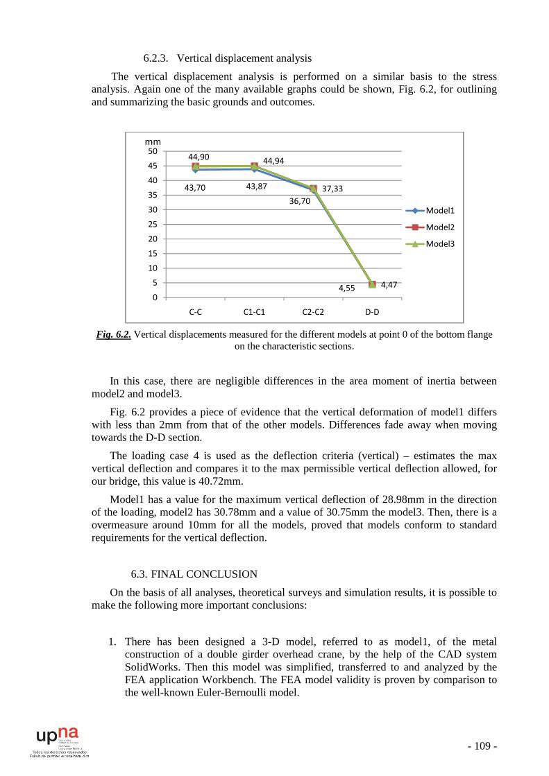
- 109 -
6.2.3. Vertical displacement analysis
The vertical displacement analysis is performed on a similar basis to the stress analysis. Again one of the many available graphs could be shown, Fig. 6.2, for outlining and summarizing the basic grounds and outcomes.
Fig. 6.2. Vertical displacements measured for the different models at point 0 of the bottom flange
on the characteristic sections.
In this case, there are negligible differences in the area moment of inertia between model2 and model3.
Fig. 6.2 provides a piece of evidence that the vertical deformation of model1 differs with less than 2mm from that of the other models. Differences fade away when moving towards the D-D section.
The loading case 4 is used as the deflection criteria (vertical) – estimates the max vertical deflection and compares it to the max permissible vertical deflection allowed, for our bridge, this value is 40.72mm.
Model1 has a value for the maximum vertical deflection of 28.98mm in the direction of the loading, model2 has 30.78mm and a value of 30.75mm the model3. Then, there is a overmeasure around 10mm for all the models, proved that models conform to standard requirements for the vertical deflection.
6.3. FINAL CONCLUSION
On the basis of all analyses, theoretical surveys and simulation results, it is possible to make the following more important conclusions:
1. There has been designed a 3-D model, referred to as model1, of the metal construction of a double girder overhead crane, by the help of the CAD system SolidWorks. Then this model was simplified, transferred to and analyzed by the FEA application Workbench. The FEA model validity is proven by comparison to the well-known Euler-Bernoulli model.
43,70 43,87
36,70
4,55
44,9044,94
37,33
4,47
0
5
10
15
20
25
30
35
40
45
50
C-C C1-C1 C2-C2 D-D
Model1
Model2
Model3
mm

- 110 -
2. The carrying metal construction of model1 is in a 3-D stressed state due to the essential influence of the connections between the main girders and end trucks as well as rotations of the supports.
3. The maximum static deformation of the 3-D model is bigger than the theoretical
one because the model takes into consideration not only the deformations due to concentrated loadings, but also the deformations due to own weight as well as twisting. In general, the metal construction of model1 is suitably constructed. It fulfills a wide range of the modern double girder overhead cranes requirements such as: modern hoist, driving units, etc. However, the mass of the model1 bridge crane could be further reduced.
4. Two models – model2 and model3 have been designed and studied as possible variants for reducing the mass of model1. The key concept of the new designs originates from the well-known idea that positioning the main girder rails over one of the main girder side plates leads to reduction in the bridge structure mass. In these new models, the structural material is used more economically in which the modified side plate has the same thickness but two types of holes are cut – simple holes and rimmed holes. These new designs succeed in reducing the model1 crane mass respectively by 5.6% and 5.4%.
5. The new design models – model2 and model3, are set to various checks in order to prove their conformity to theoretical considerations and prove that their static response is similar to that of the original crane. The varieties of checks go primarily through stress analyses, horizontal and vertical deflection analyses of the bridge. The models proved to conform to theory and their static structural response preserves the response of the original crane structure.

- 111 -
Fig.6.3. Model2 is one of the options to reduce the bridge mass
- 112 -
7. REFERENCES
[1]. Kolarov I. et al., Designing load-handling machines, Sofia, 1986
[2]. Gohberg M. M., Metal structures of materials handling machines, Leningrad, 1978
[3]. Kolarov I. Metal structures of materials handling and building machines, Sofia , 1987
[4]. Petkov G. et al., Experimental studies of materials handling machines, Sofia, 1980
[5]. Kolarov I., N. Kotzev, S. Stoychev, Metal structures of materials handling and building machines, Sofia, 1990.
[6]. Yanakiev A., M. Georgiev, , Modeling of materials handling machines and systems, Sofia, 1996
[7]. ANSYS, Theory Reference
[8]. Sumtzov A. A. et al., Results of bridge cranes gauging experiments, 1970
[9]. Cook R., Finite Element Modeling for Stress Analysis, John Wiley & Sons, 1995
[10]. SolidWorks, User’s guide, 2007
[11]. Matt Lombard, SolidWorks Bible, Wiley Publishing, 2009
[12]. CMAA Specification No. 70 (Top Running Bridge and Gantry Type Multiple Girder Electric Overhead Traveling Cranes)
[13]. OSHA Par. 1910.179 Overhead & Gantry Cranes
[14]. ASME B30.17 - 2003 Overhead and Gantry Cranes (Top Running Bridge, Single Girder, Underhung Hoist)
[15]. FEM 9.751 Power Driven Series Hoist Mechanisms, Safety
[16]. FEM 9.901 Rules for the Design of Series Lifting Equipment and Cranes Equipped with Series Lifting Equipment
[17]. Ivanchenko, F., Designing and calculating materials handling machines, Kiev, 1983
[18]. Pavlov, N, Cranes calculations examples, Mechanical engineering, 1976
[19]. Slavchev Y., Research on Carrying Metal Structure of Overhead Bridge Cranes, Lambert Academic Publishing, ISBN 978-3-8433-5644-2, 2010, Saarbrücken, Deutschland
[20]. Unstetigforder 2, von Prof. Dr. Ing. habil M. Scheffler, et al., VEB VERLAG Technik Berlin
[21]. Gere and Timoshenko, Mechanics of materials, Chapman & Hall, ISBN 0-412-36880-3, London, Third edition 1992

Abstract: The carrying metal structure (the main girders) of an actual double girder bridge crane is
modeled in 3-D and simulation research is performed for establishing the crane stressed state. Different operating modes are simulated. The stressed-state analysis includes studies of stresses at specific points on main girder cross-sections as well as frequencies and deformations. The received results are compared to similar ones from simulations of lightweight models of modified structures. The modified structures preserve the values for the height and inertia of the cross-section of the actual girders. The modified models decrease with approx. 5.5% the mass of the actual structure.
1. Introduction Bridge cranes are among the most popular material-handling machines and are applied mainly in handling
payload flows, loading/unloading and transport operations in workshops, etc. The carrying metal structure of the bridge cranes is one of their primary components. At present, the
solid-walled metal structures are among the most widely used. However, a major drawback of their design is the increased mass, particularly the main girders mass, which constitutes from 35% to 75% of the total crane mass, etc.
In this connection, the majority of the theoretical and experimental studies, dealing with reduction of structural mass, are oriented towards optimization of the main girders cross-section,etc.
The 3-D computer models turn out to be one of the most appropriate modern ways of performing reliable simulation research on the crane structures. Their popularity is due to the fact that they are much cheaper compared to the strain-gauging experiments and as well offer means of investigating the crane response at points that are almost inaccessible.
The objective of the current work is to carry out simulation researches on 3-D models of crane carrying structures in order to achieve reduction in the mass of an actual double girder bridge crane.
For fulfillment of the objective, an actual double girder crane is modeled and its response is simulated in 3-D so as to determine the crane stressed-state. Structural stresses, frequencies and deformations are analyzed and compared to theoretically obtained values.
Moreover, 3-D modeling and simulation is performed on structures that help reduce the mass of the actual crane. The lightweight models responses are compared to the response of the actual crane, keeping track of not having significant differences for similar modes of operation
2. Theoretical part
2.1. Generating 3-D models The CAD system SolidWorks is used to construct the 3-D model, of a double girder overhead crane,
produced by Kranostroene Engineering – Sofia, with main load capacity 50tonnes, and the following parameters: metal structure – deadweight 28173kg, span 28500mm, wheelbase 4600mm main girder – height 1535mm, width 500mm, second moments of inertia Jz=0.0199m4, Jy=0.0016m4 (incl. the rail), sectional area A = 506.21cm2, centroid coords yc1 = 10.95cm, zc1=0, Fig. 11.
This model is indexed as model1 but the crane structure it represents is reported as heavy and possible
researches could help in generating some lightweight modifications. For this purpose, two models are designed – model2 and model3. The key concept of the new designs
originates from the well-known idea that positioning the main girder rails over one of the main girder side plates leads to reduction in the structural mass of the bridge. It is due to the fact that the material is used more economically since the light-loaded side plate is made thinner.
Model2 and model3 are designed with one and the same girder holes, that differ only in the technology of manufacture – simple and rimmed holes, and the girder height of 1535mm is kept the same as in model1.
2.2. Models validation After the 3-D geometry is generated, it is transferred to the FEA application ANSYS Workbench for
validation as well stress and deformation analyses under applied boundary conditions. Model1 validity is confirmed in two ways:
- its displacement is compared with the displacement of an ANSYS basic beam model based on the widely accepted Euler-Bernoulli simply supported beam model which underlies the engineering check foundations of bridge cranes; - the crane static response is compared with predefined and standardized deflection criteria (horizontal and vertical).
The deflection criteria are based on standard loading cases and predetermined values. Models 2 and 3 go through the same validation.
3. Simulations with the 3-D models – results and analyses
3.1. Model1 When properly meshed and the proper boundary conditions, loadings and material properties are set, the
3-D models meshed with solid elements could reveal a detailed picture of the complex stressed state of the structure.
Loading case 1
Accounts for the live load vertical deflection of the structure. Includes crab and bridge weights and rated
load. Used to define endangered points on the structure.
Designations are:
C-C, C1-C1, C2-C2 and D-D – studied main girder cross-sections for 1 625 mma , 2 8755 mma ,
3 590 mma Main girders parameters are shown in Fig. 1, where C1 is the centroid.
TECHNICAL UNIVERSITY - SOFIA ENGLISH LANGUAGE FACULTY OF ENGINEERING
MODELLING AND SIMULATION RESEARCH ON THE METAL STRUCTURE OF BRIDGE CRANES

m
s
It is evidEq=98.05 Mmidst but is
For p.0 fupport, D-D
Fig.
Fig. 3 E
Fig. 4 Equi
ent from FiMPa. It conlocated und
from the difD section, w
1 Main girde
Equivalent s
ivalent stres
ig. that thenfirms the thder the wheefferent secti
which prove
er cross-secti
stresses Eq
sses Eq at t
e max stressheoretical vel of highesions, Fig. s again the
ion
q at bottom f
the bottom f
ses are locavalidation ost loading. 4, the equivmodel valid
Fig. 2 Me
flange point
flange point
ated at C1-Cf model1 th
valent stresdity.
as. points fro
ts from mai
t 0 for the m
C1 point5, uhat the max
sses Eq dec
om the girder
in girder sec
measured se
under the crx moment is
crease to 17
r section
ctions
ections
rab wheel, s not in the
7.51 MPa n
and are e bridge
near the
Modmodel gerrors o
The ZU L
The max def
The
reported 3.2.Both
model1 Mod
obtained
4. C
GeneModels stressed
The technoloapprox.
It is modified
Aut
del1 validitygenerated inof 1.41% in
Loadingcrane co/ 600 47L
Loadingcrane is cheflection m
YU
Loadingcrane verti
d value is U
Model2 anh models su response u
del2 and mod.
Conclusion
erated are 3-are checkedand deformamodified m
ogy of manu5.5%. confirmed
d models pre
thor: JaviePublic U
Te
y is also conn ANSYS adeflection a
g case 2 omplies wi7.5mm and t
g case 3 ecked with max 51.4m
g case 4 ical deflect
max 28.98YU
nd model3 uggest waysunchanged.odel3 are al
-D models od for validityation state of
models are deufacture – si
that the modeserve the sta
er IzurriagaUniversity oelecommuni
nfirmed by and based onand 0.82% i
ith the hothe real one
125% of themm , max eq
tion is chec
8mm
s of reduci
lso proved
Fig. 5 Mod
f an actual dy and compaf the crane isesigned with imple and r
dified modelatic response
a Lerga of Navarre –ications, 31
comparing n the Euler-in the first v
orizontal de is 10.1mm
e rated loadquivalent str
cked. The a
ng the cran
as valid by
el2 section
double girderared with th analyzed byone and the
immed hole
ls are valid e of the actua
– Pamplona006 Pamplo
crane defle-Bernoulli svertical freq
deformationm
d. The simulress max
Eq
allowable v
ne mass bu
y all the fou
F
r bridge cranhe simply suy the finite ele same type es. It is estab
with respectal crane unde
a, Technicalona, Spain.
ection and fsimply suppq are insigni
n criteria.
lation report118.1MPa
value is U
ut at the sam
ur loading c
Fig. 6 Model3
e as well as mupported Eullement methoof rectangulablished that
t to the theoer the same lo
l School for E-mail: jav
frequency vported beamificant.
The allow
rts the follow
/ 700YU L
me time ke
cases. Agai
3 section
modified moler-Bernoulliod. ar main girdthe structur
oretical consioading condi
r Industrial Evizu_10@ho
values with m. It is obser
wable defo
wing:
0 40.72mm
eeping the a
n numerous
odels of bridgbeam mode
der holes thatral mass is r
iderations. Mitions.
Engineeringotmail.com
values fromrved that th
ormation i
m . The max
actual cran
s results ar
dge structuresel. The stati
t differ in threduced with
Moreover, th
g and
m e
s
x
e
e
s. c
e h
e

I would like to express my appreciation to the reviewer – doctor Chankov, for his detailed inquiry of my project. Now for the remarks. Remark1: I agree that the surface contact elements in the 3-D models are really making the solution heavier and that the crab is not part of the project objectives and could be modeled by the reaction forces. However, we used it as a 3-D geometry because during the research the bridge crane was set to a modal analysis, where the role of the simplified crab geometry could not be fully neglected. Remark2: I agree that the shell finite elements could be used instead so as to make the solution much more effective. It could be done for future investigations, since the procedure for generating mixed-mode contacts, i.e. shell-to-solid elements will cause some more detailed attention. Remark3: I agree that the zones of local stresses and deformations could be a matter of investigation in further studies. Question1: Truly real-life experiments seem to be one of the most reliable tools for verifying the models. Probably, the most popular methods include the strain-gauging experiments. These experiments employ different tensometers and specialized devices like analog-to-digital converters, etc that enable the researcher to obtain real-life data and analyze it. Question2: The accuracy of the 3-D FE models could be checked for example by generating different meshes and solving the models with these different meshes. Some of the meshes could be denser, other - sparser until an acceptable level of the error is achieved through the iterations. Mistakes: 1) page85 - it is not fig 5.22 but fig.6.22 2) page90 - the equivalent stress of the girder is not 282.5MPa, but about 120MPA 3) page 102 - fig 6.3618

Supervisor StudentAssist.Prof. PhD Ya. Slavchev Javier Izurriaga Lerga

Cranes are industrial machines that are mainly used for materials movements inconstruction sites, production halls, assembly lines, etc.
For high capacities, over 30 tons, usuallyelectric overhead cranes (EOT) are the preferredtype, especially the double girder bridge cranes.
Crane features, like span, capacity, etcvary widely according to their weight,load type, location, etc.
Double Girder Bridge Crane ‐ The crane consists of two bridge girders supported on
two end trucks.

Double Girder Cranes
• Double girder cranes are faster, withmaximum bridge speeds up to 100 mpm,.
• They can lift up to 100 tonnes.
• They are highly suitable where thecrane needs to be fitted with specialequipment.
Usually the mass of these cranes is too high

The objective of this project is to reduce the structural mass of a real-worlddouble girder overhead crane, produced by Kranostroene Engineering – Sofia,through the use of modern computer modeling and simulation methods andapplications.
For the fulfillment of the objective, the following tasks are defined.
- accumulation of specific awareness of modern computer modeling andsimulation tools and specific applications, such as SolidWorks, ANSYS,Workbench and the Finite Element Method;
- 3-D modeling and static structural simulations of a double girder overheadcrane in order to establish its detailed 3-D structural response;
- generating models of reduced crane mass and provide evidence that theyconform to standard requirements and do not deviate significantly from theoriginal crane response.

Chapter2 is concerned with performing major engineering stress and straincalculations of the objective crane produced by Kranostroene Engineering –Sofia. Since the objective is to reduce the crane mass mainly through thedecrease in the mass of the main girders, these girders are of major importancefor the computations
A solid walled bridge construction is considered, where the main girders arewelded to the end trucks. Some of the major crane parameters are shown in thetable

Here are briefly shown some calculations performed according to the first calculationscheme - sharp load lift at stationary crane
The I-st calculation scheme is according to the figure.

The project objective requires that modern computer modeling and simulation methodsand applications be used.
The finite element method (FEM), sometimes referred to as finite element analysis (FEA),is a computational technique used to obtain approximate solutions of boundary valueproblems in engineering.
The current physical problem being analyzed is that of mechanical engineering and thefield variable is the physical displacement
There exist different FEA applications but the current interest is towards one of the mostpopular – ANSYS and ANSYS Workbench.
Workbench is quite powerful indealing with 3-D geometries, it could beemployed in studying the structuralcrane behavior using elements likeSOLID186.
SOLID186 structural solid is wellsuited to modeling irregular meshes(such as those produced by variousCAD/CAM systems). The element mayhave any spatial orientation.

Chapter 4 deals with generation of 3-Dmodels.
The CAD system SolidWorks is usedto construct the 3-D model, of a doublegirder overhead crane, produced byKranostroene Engineering – Sofia, withmain load capacity 50tonnes, and thefollowing parameters for the metalstructure
deadweight 28173kg,span 28500mm,wheelbase 4600mm
The bridge structure itself consists ofseveral assemblies:
main girdersend truckscrane driving units
This model is indexed as model1.
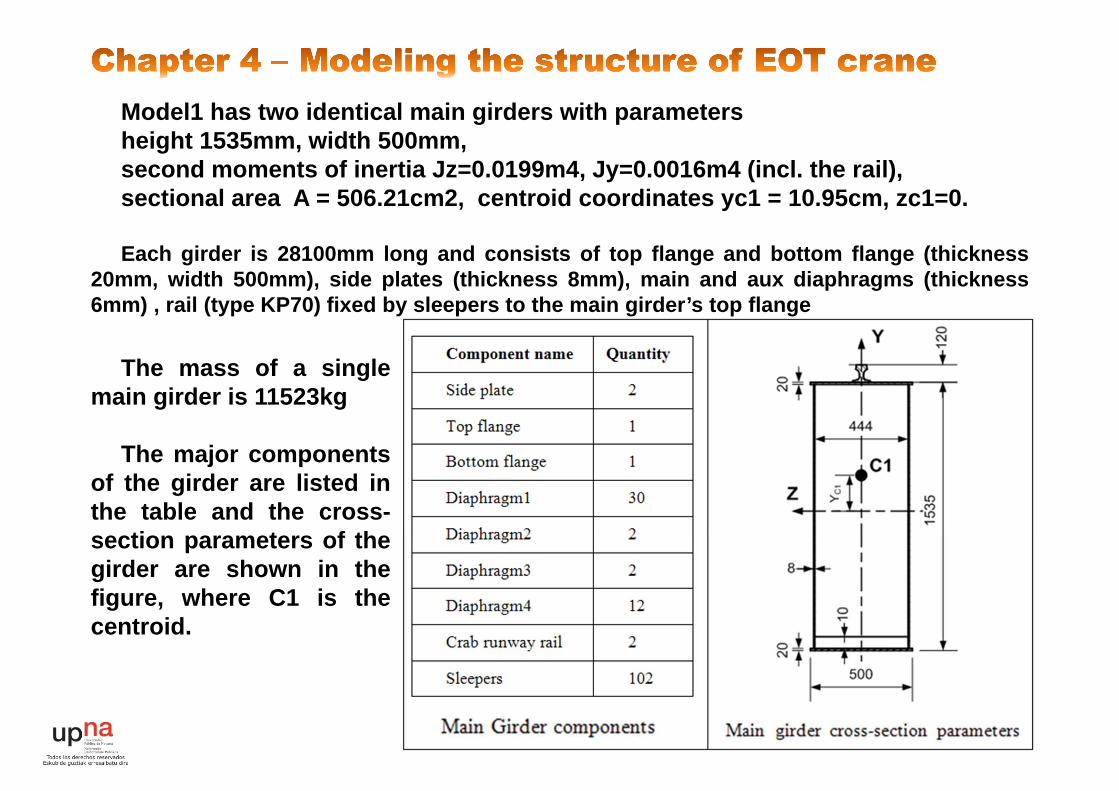
Model1 has two identical main girders with parametersheight 1535mm, width 500mm,second moments of inertia Jz=0.0199m4, Jy=0.0016m4 (incl. the rail),sectional area A = 506.21cm2, centroid coordinates yc1 = 10.95cm, zc1=0.
Each girder is 28100mm long and consists of top flange and bottom flange (thickness20mm, width 500mm), side plates (thickness 8mm), main and aux diaphragms (thickness6mm) , rail (type KP70) fixed by sleepers to the main girder’s top flange
The mass of a singlemain girder is 11523kg
The major componentsof the girder are listed inthe table and the cross-section parameters of thegirder are shown in thefigure, where C1 is thecentroid.

The crane runway rails (KP-80)and the crab runway rails (KP-70)are designed according to thestandardized requirements for thedimensions, as shown.
Moreover, these rails aredesigned through the use of thedesign table method, available inSolidWorks.
A design table allows you tobuild multiple configurations ofparts or assemblies by specifyingparameters in an embeddedMicrosoft Excel worksheet.

The crane structure in model1 is heavy.Two models are designed –
model2 and model3.
The key concept of the newdesigns - position the maingirder rails over one of the maingirder side plates to reduce thestructural mass of the bridge. Itis due to the fact that thematerial is used moreeconomically since the light-loaded side plate is madethinner.
Model2 and model3 aredesigned with one and the samegirder holes, that differ only inthe technology of manufacture –simple and rimmed holes, andthe girder height of 1535mm iskept the same as in model1.

The sheet metal forming tools in SolidWorks (and more specifically theextruded flanges) is the method applied here for creating the rimmed holes shownin the figure.
The sheet metal featuresallow the design of complexshapes and the repetitive use ofconfigurations through thelibrary features.
Library features are featuresthat you create once and re-usemany times. They are intendedto be parametrically flexible tofit into many types of geometry,but they can also be of a fixedsize and shape.
One very useful aspect of library features is that they can be driven byconfigurations and design tables. Once the feature is in the part, theconfigurations are still available, and so you can change the configuration of anapplied library feature at any time.

All three models have their main girder mid cross-section parameters as shown
Jz, Jy – measured with respect to corresponding point CThe total mass reduction for both girders: model2 – 1286kg, model3 – 1234kg
It is evident that model 1 has the heavies girder – 11523kg. The introduction of the newmain girder design, through model 2 and 3 lightens the girder with an average of 5.5%. Itmeans that the crane mass could be decreased with 1200 to 1300kg, by just making thesemain girder redesign procedures.
The table shows also that the new designs follow closely the parameters of the basiccrane model.
However, the stress response must be checked and it could be done by the FE method.

All models generated in chapter 4 are analyzed in chapter 5 using the FE method.
Analyses include stresses, deformations, frequencies, etc.
Validity confirmation:- Displacement compared with the displacement of the widely accepted Euler-Bernoulli
simply supported beam model, prepared as an ANSYS model;- Crane static response compared with standardized deflection criteria
The majority of possible structural loadings is classified into several cases:
Loading case 1 (LC1) – Live load vertical deflection of the structure.
Loading case 2 (LC2) – Deflection criteria (horizontal).
Loading case 3 (LC3) – Crane testing requirement with 125% of rated load capacity.
Loading case 4 (LC4) – Deflection criteria (vertical).
Thus, the bridge structure is checked for conformity with horizontal and verticaldeflection criteria, overloading and live loads as defined in the engineering standards.
Model2 and model3 crane static response is to be compared with the model1 responsefor any significant deviations from the response of the original crane.

Model1 preparation for simulation
•20-Node Quadratic Wedge
38962 finite elements and 72937 nodes.•10-Node Quadratic Tetrahedron Solid187•20-Node Quadratic Hexahedron
•Quadratic Quadrilateral Contact•Surface Contact Target;
•Hi-order Surface to SurfaceContact
Model1 results
Model1 vs ANSYS
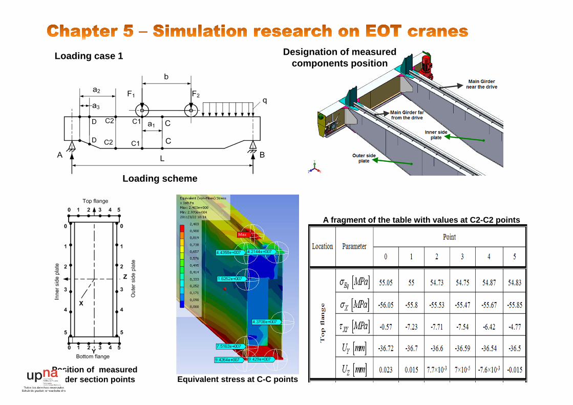
Loading case 1
Loading scheme
Designation of measured components position
Position of measured girder section points Equivalent stress at C-C points
A fragment of the table with values at C2-C2 points

Loading case 1
Equivalent stress at section D-D
Loading case 1 analyses
Eq stress at points of bottom flange along the characteristic sections of the beam
Equivalent stresses at point 0 of bottom flange
Stresses at differentbottom flange points remainalmost unchanged for thecorresponding section.However, the stress values atthe same point in the differentsections tend to vary as shown
The reported stress in themiddle cross section is high(94.67MPa) and this value iseven higher in section C1-C1,reaching up to 97.73 MPa.Comparison among the maxstress values of all the sectionsyielded that the critical sectionis under the crab wheel.
Stress values go down to17.51MPa in the section nearthe end truck, which againconforms to the strength ofmaterials postulates.

Loading case 2
Loading schemeThe horizontal loading is applied as horizontal
acceleration
max2 0.102 5 50 'ag
o
20.5 /a m s
Due to horizontal loading, payload swingsfrom vertical according to:
Horizontal deflection of the crane structure
Max. values at section C-C
For this case, the bridgespan is L=28500mm, thenL/600=47.5mm.
As shown in the table,the max deflection Uz,max[mm] is below the 47.5mmvalue and it follows that thecrane conforms to thisrigidity requirement.

Equivalent stress at section C1-C1, model 2
Equivalent stress at section C2-C2 model 3

LOADING CASE 1

Model2, outer side plate, section C2-C2, equivalent stress and deformed shape (the view is scaled 200 times)
Model3, outer side plate, section C2-C2, equivalent stress and deformed shape (the view is scaled 200 times)

Eq stresses measured for the different models at point 0 of the bottom flange on the characteristic sections.
STRESS SUMMARY DISPLACEMENT SUMMARY
Vertical displacements at point 0 of the bottom flange on the characteristic sections

On the basis of all analyses, theoretical surveys and simulation results, it is possible to make the following more important conclusions:
1) There has been designed a 3-D model, referred to as model1, of the metal construction of a doublegirder overhead crane. The FEA model validity is proven by comparison to the well-known Euler-Bernoulli model.
2) The carrying metal construction of model1 is in a 3-D stressed state due to the essential influenceof the connections between the main girders and end trucks as well as rotations of the supports.
3) In general, the metal construction of model1 is suitably constructed. It fulfills a wide range of themodern double girder overhead cranes requirements such as: modern hoist, driving units, etc.However, the mass of the model1 bridge crane could be further reduced.
4) Two models – model2 and model3 have been designed and studied as possible variants forreducing the mass of model1. The key concept of the new designs originates from the well-knownidea that positioning the main girder rails over one of the main girder side plates leads toreduction in the bridge structure mass. In these new models, the structural material is used moreeconomically in which the modified side plate has the same thickness but two types of holes arecut – simple holes and rimmed holes. These new designs succeed in reducing the model1 cranemass respectively by 5.6% and 5.4%.
5) The new design models – model2 and model3, are set to various checks in order to prove theirconformity to theoretical considerations and prove that their static response is similar to that ofthe original crane. The varieties of checks go primarily through stress analyses, horizontal andvertical deflection analyses of the bridge. The models proved to conform to theory and their staticstructural response preserves the response of the original crane structure.