Research Paper Efﬁcient computation of exposure proﬁles … · 2017-01-16 · and the percentage of loss given default ... portfolio to mitigate the credit risk that arises from

Journal of Computational Finance 20(1), 139–172DOI: 10.21314/JCF.2017.337

Research Paper

Efficient computation of exposure profiles onreal-world and risk-neutral scenarios forBermudan swaptions

Qian Feng,1 Shashi Jain,3 Patrik Karlsson,3

Drona Kandhai3,4 and Cornelis W. Oosterlee1,2

1Centrum Wiskunde and Informatica (CWI), Science Park 123, 1098 XG Amsterdam,The Netherlands; emails: [email protected], [email protected] University of Technology, Mekelweg 4, 2628 CD Delft, The Netherlands3ING Bank, Foppingadreef 7, PO Box 1800, 1000 BV Amsterdam, The Netherlands;emails: [email protected], [email protected] of Amsterdam, PO Box 94216, 1090 GE, Amsterdam, The Netherlands;email: [email protected]

(Received June 6, 2016; accepted June 7, 2016)

ABSTRACT

This paper presents a computationally efficient technique for the computation ofexposure distributions at any future time under the risk-neutral and some observedreal-world probability measures; these are needed for the computation of credit valua-tion adjustment (CVA) and potential future exposure (PFE). In particular, we present avaluation framework for Bermudan swaptions. The essential idea is to approximate therequired value function via a set of risk-neutral scenarios and use this approximatedvalue function on the set of observed real-world scenarios. This technique signifi-cantly improves the computational efficiency by avoiding nested Monte Carlo simu-lation and using only basic methods such as regression. We demonstrate the benefits

Corresponding author: Q. Feng Print ISSN 1460-1559 jOnline ISSN 1755-2850Copyright © 2016 Incisive Risk Information (IP) Limited

139

140 Q. Feng et al

of this technique by computing exposure distributions for Bermudan swaptions underthe Hull–White and G2++ models.

Keywords: credit valuation adjustment (CVA); credit exposure; potential future exposure (PFE);Bermudan swaption; risk-neutral measure; real-world measure.

1 INTRODUCTION

The aim of the regulatory capital base in the Basel framework is to improve a bank’sresilience against future losses due to defaults of counterparties (Basel Committee onBanking Supervision 2010). Credit exposure to counterparties occurs due to financialtransactions or investments via over-the-counter (OTC) derivatives products. It isdefined as the market value of the replacement costs of transactions if a counterpartydefaults, assuming no recovery. Banks are required to hold regulatory capital to backexposure in the future to all their counterparties.

The Basel Committee gives specific definitions for the credit exposure metricsand adjustments regarding the future credit risk to banks/firms (Basel Committee onBanking Supervision 2005). For example, the expected exposure (EE) is the mean ofthe exposure distribution at any particular future date. The potential future exposure(PFE) is a high quantile (typically 97% or 99%) of the exposure distribution at anyparticular future date. The (unilateral) credit valuation adjustment (CVA) is the marketvalue of the credit risk of the counterparty to the bank, which is typically calculatedvia an integral over time of the product of the discounted EE, the default probabilityand the percentage of loss given default (LGD) (Zhu and Pykhtin 2007).

EE and PFE are important indicators for the safety of a bank’s portfolio to marketmovements. They are therefore used as metrics for capital requirements by regulatorsin Basel II and III (Gregory 2010). PFE is used for trading limits for portfolios withcounterparties, as it may indicate at any future date the maximum amount of exposurewith a predefined confidence. For example, the 99% PFE is the level of potentialexposure that can be exceeded with a probability of 1%. CVA is a charge that hasa direct impact on the balance sheet and the income statement of a firm, as it is anadjustment to the value of financial derivatives.

There are three basic steps in calculating future distributions of exposure (Gregory2010):

� the generation of scenarios using the models that represent the evolution of theunderlying market factors;

� the valuation of the portfolio for each scenario at each monitoring date;

� the determination of exposure values at each date for each scenario.

Journal of Computational Finance www.risk.net/journal

Efficient computation of exposure profiles 141

There is no doubt that CVA must be computed under the risk-neutral measure, as itis the market price of counterparty default risk. It is the cost of setting up a hedgeportfolio to mitigate the credit risk that arises from exposure against a counterparty.In the setting of a CVA computation, scenarios are generated under the risk-neutralmeasure to compute “risk-neutral exposure distributions”.

In contrast, for risk analysis, it is argued that expectations (EEs) and quantiles(PFEs) of future exposure values must be obtained via scenarios that can reflect thereal world in a realistic way. We know that the risk-neutral probability measure usedin the pricing process does not reflect the real-world probability of future outcomes, asit has been adjusted based on the assumption that market participants are risk neutral.

The Girsanov theorem states that the risk-neutral volatility should be equal tothe real-world volatility when an equivalent measure exists (Andersen and Piterbarg2010). However, it is well known that in practice the risk-neutral market-impliedvolatility differs from the observed real-world volatility (Hull et al 2014; Stein2013). The observed historical dynamics and the calibrated risk-neutral dynamicsmay exhibit a different behavior, which is a challenge for risk management, as thecomputational cost becomes high.

In practice, calculation of exposure values on each real-world scenario at eachmonitoring date needs to be performed under a risk-neutral measure. For certainproducts, such as Bermudan swaptions, the valuation is based on Monte Carlo simu-lations, which can be computationally intensive, especially since pricing then requiresanother nested set of Monte Carlo paths. The computational cost increases drasticallydue to the number of real-world scenarios, risk-neutral paths and monitoring dates.

Employing a simplification, ie, assuming that the observed real-world scenariosare close to the risk-neutral scenarios and calculation takes place under just onemeasure, may lead to serious problems, as there are significant differences betweenthe resulting distributions. Stein (2014) showed that exposures computed under therisk-neutral measure depend on the choice of numéraire and can be manipulated bychoosing a different numéraire. As a conclusion, it is crucial that calculations of EEand PFE are done under the real-world instead of the risk-neutral measure.

The computational problem poses a great challenge to practitioners to enhancecomputational efficiency.Available solutions include reduction of the number of mon-itoring dates and Monte Carlo paths, application of variance reduction techniques andusing interpolation and enhanced computational platforms such as graphics process-ing units (GPUs). Even with all these efforts, calculations cost a lot of time (Stein2014).

For Bermudan swaptions, Joshi and Kwon (2016) provided an efficient approachfor approximating CVA, which relies only on an indicator of future exercise time alongscenarios, the decision of which is based on the regressed functions. The expected

www.risk.net/journal Journal of Computational Finance

142 Q. Feng et al

exposure at a monitoring date is then obtained from the corresponding deflated path-wise cashflows. However, this approximation method cannot, in a straightforwardfashion, be used for PFE on the real-world scenarios. For PFE computations, Stein(2013) proposed to avoid nested Monte Carlo simulations by combining the real-world and the risk-neutral probability measures. The computed results lie betweenthe computed PFE values under the real-world and risk-neutral probability measures.

In this paper, we will focus on accurate computation of these risk measures fora heavily traded OTC derivative, the Bermudan swaption. There are well-developedmethods that can be used to compute the time-zero value of Bermudan swaptions,such as regression and simulation-based Monte Carlo methods, eg, the least squaresmethod (LSM) (Andersen 1999; Longstaff and Schwartz 2001) or the stochastic gridbundling method (SGBM) (Jain and Oosterlee 2012, 2015; Karlsson et al 2014), thefinite difference (FD) PDE method or the Fourier expansion-based COS method (Fangand Oosterlee 2009).

This paper presents an efficient method to significantly enhance the computationalefficiency of exposure values computation without the nested simulation. The key isto approximate the value function by a linear combination of basis functions obtainedby risk-neutral scenarios, and to compute the expected payoff using the approximatedvalue function to determine the optimal early exercise strategy on the paths repre-senting the observed real-world scenarios. Only two sets of scenarios, one under therisk-neutral and one under the observed historical dynamics, are needed to computethe exposure distributions at any future time under the two measures. We apply thisnumerical scheme within the context of the LSM and SGBM approaches.

The paper is organized as follows. Section 2 presents the background mathematicalformulation of EE, PFE and CVA as well as the dynamic programming framework forpricing Bermudan swaptions. Section 3 explains the essential insight for computationunder two measures based on the risk-neutral scenarios, and describes the algorithmsfor computing the exposure profiles for the SGBM and LSM. We provide referencevalues for exposure, based on Fourier-cosine expansions, in Section 4. Section 5presents numerical results with the algorithms developed for the one-factor Hull–White and two-factor G2++ models.

2 CREDIT VALUATION ADJUSTMENT, EXPECTED EXPOSURE ANDPOTENTIAL FUTURE EXPOSURE AS RISK MEASURES

In this section, we present the general framework for computing the exposure mea-surements. It is important to choose suitable probability measures to compute CVA,EE and PFE. We will discuss the practical background and the choice of probabilitymeasures.



2.1 Calibration and backtesting

It is well known that there are differences between calibrated historical dynamicsand the dynamics implied by market prices. The reason is that models calibratedto historical data tend to reflect future values based on historical observations, andmodels calibrated to market prices reflect market participants’ expectations about thefuture. Some research on building a joint framework in the real and risk-neutral worldsis done by Hull et al (2014). They propose a joint measure model for the short rate,in which both historical data and market prices can be used for calibration, and thecalibrated risk-neutral and real-world measures are equivalent.

The practical setting with respect to calibrating model parameters is involved,however. Backtesting of counterparty risk models is required by the Basel Committeefor those banks with an internal model method approval, for which PFE is an importantindicator for setting limits. Backtesting refers to comparison of the outcomes of abank’s model against realized values in the past. The bank’s model must be consistentwith regulatory constraints; in other words, it must be able to pass the backtestingof PFE. A bank has to strike a balance between managing its risk and meeting theexpectations of the shareholders. An overconservative estimate of market factors forexposure computation would lead to high regulatory capital reservings.

In short, a model used by a bank for generating scenarios should be able to reflectthe real world: it should be able to meet the requirements of backtesting limits byregulators and the return rate by investors. Based on this, Kenyon et al (2015) proposeda risk-appetite measure that would fit in with these requirements. When a calibratedmodel under this risk-appetite measure cannot pass the backtesting, the bank needsto reconsider its preferences. From backtesting, one may find a so-called PFE-limitimplied volatility of a model, by which, combined with a given budget, a bank’s riskpreference can be computed.

Ruiz (2012) called the model that describes the evolution of the underlying marketfactors the risk factor evolution (RFE) model, on which the backtesting is done peri-odically. The related probability measure is called the RFE measure. In that work, themodel used to describe the real world is introduced first, and the relevant probabilitymeasure is defined based on the model. In some sense, there are different probabilitymeasures induced by the backtesting setting that describe the outcome, assuming theunderlying factors evolve according to the calibrated model.

2.2 Mathematical formulation

Consider an economy within a finite time horizon Œ0; T �. The probability space.˝;F ;P/ describes the uncertainty and information, with ˝ being the samplespace consisting of outcome elements w, with F being a � -algebra on ˝, and withP W F ! Œ0; 1� being the probability measure that specifies the probability of events


144 Q. Feng et al

happening on the measure space .˝;F /. Information up to time t is included in thefiltration fFt ; t 2 Œ0; T �g.

Further assume a complete market without arbitrage opportunities. There exists anequivalent martingale measure such that a price associated to any attainable claimis computed as an expectation under this probability measure with respect to theassociated numéraire. We choose to use a risk-neutral probability measure, denotedby Q W F ! Œ0; 1�, with numéraire Bt .w/ D exp.

R t0rs.w/ ds/, where frs; s 2 Œ0; t �g

is the risk-neutral short rate. The numéraire Bt represents a savings account withB0.w/ D 1.

Inspired by Kenyon et al (2015) and Ruiz (2012), we define a probability measure ofobserved history that can pass the backtesting. We use the notation A W ˝ 0 ! Œ0; 1� topresent the observed historical probability measure on some measure space .˝ 0;F 0/that we choose to reflect the probability of events in the real world. The probabilitymeasure A.˝ 0/ D 1. The observed historical measure A may not be equivalent to thechosen risk-neutral measure Q.As a probability space that includes realized outcomesin the past, the observed measure space should satisfy ˝ 0 � ˝ and the associatedfiltration F 0t � Ft .

Let the stochastic process fXt 2 Rd ; t 2 Œ0; T �g on .˝;F / represent all influentialmarket factors. We further define the market factor fXtgT0 on the space .˝ 0;F 0/ asthe same mapping as the one on .˝;F /, ie, for an outcomew that may happen in both˝ and ˝ 0 with different probability, one will have the same realized values for themarket factors. Fixing an outcome w 2 ˝ 0 � ˝, the stochastic process is a functionof time t , ie, Xt .w/ W Œ0; T �! Rd , which is a path of Xt .

2.3 Definition of exposure, credit valuation adjustment andpotential future exposure

Let the value of a portfolio v at time t be denoted by random variable vt W ˝ ! R;vt .w/ is the value of the portfolio at time t on a path, which is the mark-to-marketvalue of the portfolio computed under the risk-neutral measure Q.

We define exposure as the replacement costs of the portfolio, given by

Et .w/ D max.0; vt .w//; (2.1)

where w 2 ˝. Once the contract expires or, in the case of early exercise options,when the contract is exercised before expiry, the exposure of the portfolio is equal tozero.

Assume the percentage of LGD to be a constant over time, and let PS.t/ representthe default probability up to time t , which is retrieved from credit default swap (CDS)market data under the risk-neutral probability measure. Assume the independence of



exposure and the probability of default. The CVA formula is then given by

CVA0 D LGDZ T

0

EE�.t/ d PS.t/; (2.2)

where the notation d PS.t/ represents the probability that the default event occursduring the interval Œt; t C dt �, and the discounted expected exposure EE� is the con-ditional expectation of discounted exposure computed with the probability measureQ, given by

EE�.t/ D EQ

�Et

Bt

�D

Z˝

Et .w/

Bt .w/dQ.w/; (2.3)

where EQ is the risk-neutral expectation.The curve PFE.t/ is a function of future time t until the expiry of the transactions

T . Its peak value indicates the maximum potential exposure of a portfolio over thehorizon Œ0; T �. We define the PFE curve at time t 2 Œ0; T � as the 99% quantile of theexposure distribution, measured by the observed probability measure A, given by

PFE.t/ D inffy j A.fw W Et .w/ < yg/ > 99%g; (2.4)

where w 2 ˝ 0 and X0.w/ D x.The maximum PFE (MPFE) is used to measure the peak value at the PFE curve

over the time horizon Œ0; T �, given by

MPFE D maxt2Œ0;T �

PFE.t/: (2.5)

In a similar way, another measure of credit risk of a portfolio is the EE, which isthe average exposure at any future date, denoted by EE.t/. The value of the EE curveat a monitoring date t under the observed measure A is given by

EE.t/ D EAŒEt � D

Z˝0Et .w/ dA.w/; (2.6)

where w 2 ˝ 0 and X0.w/ D x. The real-world expected positive exposure (EPE)over a time period Œ0; T � is given by

EPE.0; T / D1

T

Z T

0

EE.t/ ds: (2.7)

In particular, we are interested in Bermudan swaptions, the pricing dynamics ofwhich are presented in the following section.


146 Q. Feng et al

2.4 Pricing of Bermudan swaptions

A Bermudan swaption is an option where the owner has the right to enter into anunderlying swap either on the swaption’s expiry or at a number of other predefinedexercise dates before the expiry date. As soon as the swaption is exercised, the under-lying swap starts. We assume here that the expiry date of the swap is predefined, sothe duration of the swap is calculated from the swaption exercise date until a fixed enddate. The underlying dynamics for the short rate governing the Bermudan swaptionare either the one-factor Hull–White model or the two-factor G2++ model. Details ofthese well-known governing dynamics, either under the risk-neutral or the observedreal-world dynamics, are presented in Appendixes 1 and 2 (available online).

We assume that the exercise dates coincide with the payment dates of the underlyingswaps. Then, we consider an increasing maturity structure, 0 < T1 < � � � < TN <

TNC1, with TNC1 the fixed end date of the underlying swap and T1; TN the first andlast opportunities to enter, respectively. We define T0 D 0. We assume that when aninvestor enters a swap at time Tn, n D 1; 2; : : : ; N , the payments of the underlyingswap will occur at TnC1; TnC2; : : : ; TNC1, with time fraction �n D TnC1�Tn. We letN0 represent the notional amount and K be the fixed strike. We use indicator ı D 1for a payer Bermudan swaption and ı D �1 for a receiver Bermudan swaption.

The payoff for entering the underlying swap at time Tn associated with paymenttimes Tn D fTnC1; : : : ; TNC1g, conditional on XTn D x, is given by (Brigo andMercurio 2007)

Un.x/ D N0

� NXkDn

P.Tn; TkC1; x/�k

�max.ı.S.Tn;Tn; x/ �K/; 0/; (2.8)

where the forward swap rate S.t;Tn; x/ at time t 6 Tn associated with timeTn; : : : ; TNC1 is defined by

S.Tn;Tn; x/ D1 � P.Tn; TNC1; x/PNkDn P.Tn; TkC1; x/�k

; (2.9)

and P.Tn; Tk; x/ is the price of a zero-coupon bond (ZCB), conditional onXTn D x,associated with times Tn and Tk . The analytic formula of the ZCB is related to therisk-neutral model for the underlying variable (see, for example, Appendixes 1 and2, available online).

We refer to a function Un, a bounded Borel function, as the exercise function,which represents the value of the future payments on any given scenario, when theoption will be exercised at time Tn. For completeness, we define U0 � 0. We choosefor the stochastic process fXt ; t 2 Œ0; TN �g an Ito diffusion. In that case, Un.XTn/



FIGURE 1 Time lines.

0 1 2 3 4 5 6 7 8 9 10

0 1 2 3 4 5 6 7 8 9 10

Exercise dates time line

Monitoring dates time line

T0 T1 T2 T3 T4 T5 T6 T7

t0 t5 t10 t15 t20 t25 t30 t35 t40 t45 t50

is a continuous variable, as XTn is a continuous random variable. The value of notexercising the option at t 2 Œ0; TN / is the value of continuing the option at time t .

Let time t 2 ŒTn; TnC1/, where the exercise opportunities are restricted to datesfTnC1; : : : ; Tng. The value of the Bermudan claim is the risk-neutral expectationof the (discounted) future payoff when exercising optimally (Øksendal 2003). Withthe strong Markov property of the Ito diffusions (Øksendal 2003), the value of thisBermudan claim at time t , conditional on Xt D x, is the value that is obtained bymaximizing the following object function (Glasserman 2003):

C.t; x/ D maxI2fnC1;:::;N g

BtEQ

�UI .XTI /

BTI

ˇ̌̌ˇ Xt D x

�; (2.10)

where n D 0; : : : ; N � 1. We refer to the value function C.t; �/ as the continuationfunction at time t .

We wish to determine the exposure at a set of discrete monitoring dates, f0 D t0 <t1 < � � � < tM D TN g, with time step �tk D tkC1 � tk , k D 0; : : : ;M � 1. Thesemonitoring dates include the exercise dates fT1; T2; : : : ; TN g, and tM is equal to TN .There are some dates between each two exercise dates, as we are also interested inthe exposure at those intermediate dates.

Figure 1 presents the time lines of the exercise dates of a Bermudan swaption andthe monitoring dates used for exposure computation as an example. This Bermudanswaption can be exercised seven times between year four and year ten, ie, year four isthe first exercise date and year ten is the expiry (the last exercise date). The exposuremonitoring dates are each one-fifth of a year from time zero until year ten. Themonitoring date t20 D 4 coincides with the first exercise date,and the monitoring datet50 D 10 is equal to the last exercise opportunity.


148 Q. Feng et al

We compute the exposure of a Bermudan claim at monitoring dates ftmgMmD0. Valuefunction V then satisfies (Glasserman 2003)

V.tm; x/ D

8̂̂<ˆ̂:UN .x/; tM D TN ;

max.C.tm; x/; Un.x//; tm D Tn; n < N;

C.tm; x/; Tn < tm < TnC1; n < N;

(2.11)

where the continuation function C is computed as the conditional expectation of thefuture option value, given by

C.tm; x/ D BtmEQ

�V.tmC1;XtmC1/

BtmC1

ˇ̌̌ˇ Xtm D x

�; (2.12)

which can be proven to be equivalent to (2.10) by induction.The optimal exercise strategy is now as follows. At state XTn D x, exercise takes

place when Un.x/ > C.Tn; x/, and the option is kept at all non-exercise monitoringdates tm. The value function V and continuation function C are defined over the timeperiod Œ0; TN � and space D 2 Rd .

The pricing dynamics in (2.11) are most conveniently handled by means of a back-ward recursive iteration. From known value UN at time tM D TN , we computeV.tM�1; �/, and subsequently function V.tM�2; �/, and so on, until time zero. Theessential problem, hence, becomes to determine the value functionV and continuationfunction C at all monitoring dates ftmgMmD1.

Remark 2.1 Given a fixed pathw0 2 ˝ 0 orw 2 ˝, we compute the option valuesfor the scenario as V.tm;Xtm.w// at any monitoring date tm by (2.11). Once theoption for scenario w is exercised at a specific date, the option terminates, and theexposure values regarding this option along the scenario from the exercise date to Tbecome zero.

When a sufficient number of scenarios for the risk-neutral model are generated,the option value can be determined at all monitoring dates for any scenario, and weobtain a matrix of exposure values called the exposure profile.

The exposure profile, computed from observed real-world scenarios that are cal-ibrated based on historical data, is an empirical real-world exposure density fromwhich we can estimate real-world EEs and PFEs at each monitoring date. However,with risk-neutral short rate processes, the exposure profiles on risk-neutral scenariosare needed to compute the discounted EE.

We see that the key to computing exposure profiles on generated scenarios is toknow the value function V and the continuation function C at all monitoring datesftmg

MmD1.

Nested Monte Carlo simulation is often used when a simulation-based algorithm isemployed for the valuation; this is expensive, as simulations of risk-neutral paths are



needed for each (real-world) scenario at each monitoring date. Suppose that accuratepricing requiresKI risk-neutral paths atM monitoring dates; then, the computationaltime would beO.M 2KIKa/ forKa real-world scenarios for computing EE and PFEprofiles.

3 REGRESSION-BASED MONTE CARLO ALGORITHMS

The computation of the conditional risk-neutral expectation is the most expensivepart in the algorithm for dynamics (2.11). We propose algorithms that can approxi-mate the continuation function in (2.12) by basic functions (for example, polynomialfunctions), based on the risk-neutral scenarios. Using these functions, we can performsimulations with risk-neutral expectations on the real-world scenarios without nestedsimulations. To compute CVA and PFE, we only need one set of Kq risk-neutralscenarios and one set of Ka real-world scenarios.

The proposed algorithms are based on the approximation of the continuation func-tion within the SGBM and LSM simulation techniques. In this section, details of thealgorithms are presented as well as the differences between the LSM and SGBM.

3.1 Stochastic grid bundling method

The SGBM approach, based on regression, bundling and simulation, was developedby Jain and Oosterlee (2015) for pricing Bermudan options. The SGBM can be verynaturally generalized toward the efficient computation of exposure profiles becauseof its high accuracy in approximating expected payoffs on each Monte Carlo path.The SGBM has been used to compute risk-neutral exposure profiles (for computingCVA) of Bermudan-style claims in Karlsson et al (2014) and Feng and Oosterlee(2014).

Pricing in the context of the SGBM approach is based on risk-neutral scenarios.Computation of discounted expected option values is performed locally in so-calledbundles by means of local regression. We will store the bundle-wise approximatedcontinuation functions and use them to compute exposure profiles for the observedreal-world scenarios for a Bermudan swaption.

3.1.1 Risk-neutral scenarios

Let fXq1;h; : : : ; X

q

M;hgKqhD1

beKq scenarios, where the underlying factor evolves withthe risk-neutral model. Pricing is done by a backward-in-time iteration, as in (2.11),from time tM to time t0 D 0.

To initialize the computation, the option value at expiry tM D TN is computed asthe immediate payoff UN , ie, the option value realized on the hth scenario at time


150 Q. Feng et al

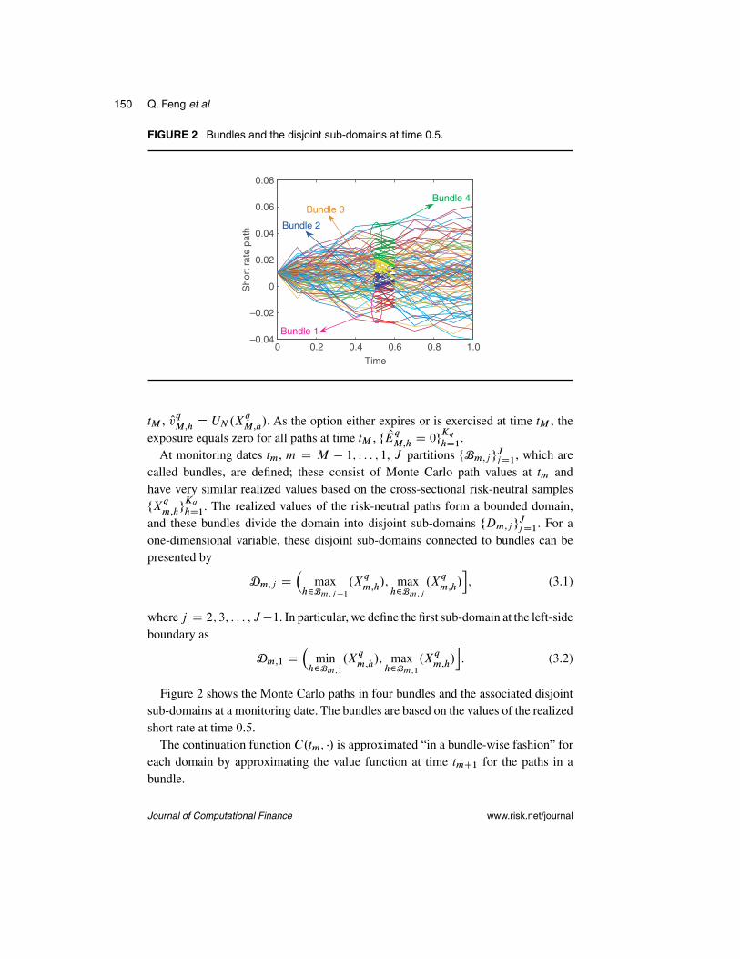
FIGURE 2 Bundles and the disjoint sub-domains at time 0.5.

Time0 0.2 0.4 0.6 0.8 1.0

Sho

rt r

ate

path

–0.04

–0.02

0

0.02

0.04

0.06

0.08

Bundle 3Bundle 4

Bundle 2

Bundle 1

tM , OvqM;hD UN .X

q

M;h/. As the option either expires or is exercised at time tM , the

exposure equals zero for all paths at time tM , f OEqM;hD 0g

KqhD1

.At monitoring dates tm, m D M � 1; : : : ; 1, J partitions fBm;j g

JjD1, which are

called bundles, are defined; these consist of Monte Carlo path values at tm andhave very similar realized values based on the cross-sectional risk-neutral samplesfX

q

m;hgKqhD1

. The realized values of the risk-neutral paths form a bounded domain,and these bundles divide the domain into disjoint sub-domains fDm;j gJjD1. For aone-dimensional variable, these disjoint sub-domains connected to bundles can bepresented by

Dm;j D�

maxh2Bm;j�1

.Xq

m;h/; maxh2Bm;j

.Xq

m;h/i; (3.1)

where j D 2; 3; : : : ; J �1. In particular, we define the first sub-domain at the left-sideboundary as

Dm;1 D�

minh2Bm;1

.Xq

m;h/; maxh2Bm;1

.Xq

m;h/i: (3.2)

Figure 2 shows the Monte Carlo paths in four bundles and the associated disjointsub-domains at a monitoring date. The bundles are based on the values of the realizedshort rate at time 0:5.

The continuation function C.tm; �/ is approximated “in a bundle-wise fashion” foreach domain by approximating the value function at time tmC1 for the paths in abundle.



For j D 1; : : : ; J , on the Monte Carlo paths in bundle Bm;j , the value functionV.tmC1; �/ is approximated by a linear combination of basis functions f�kgBkD1, ie,

V.tmC1; y/ �

BXkD1

ˇk.m; j /�k.y/; (3.3)

where the coefficientsˇk.m; j / of the kth basis function minimize the sum of squaredresiduals over the paths in bundle Bm;j , ie,

Xh2Bmj

�Ovq

mC1;h�

BXkD1

ˇk.m; j /�k.Xq

mC1;h/

�2; (3.4)

with f OvqmC1;h

gKqhD1

the option values at time tmC1 on the cross-sectional sample

fXq

mC1;hgKqhD1

.Using the approximated value function in (3.3) instead of the “true value” in (2.12),

the continuation function on Dm;j can be approximated by

C.tm; x/ �

BXkD1

ˇk.m; j / k.x; tm; tmC1/; (3.5)

where x 2 Dm;j and function k is the conditional risk-neutral discountedexpectation of basis function �k , defined by

k.x; tm; tmC1/ WD BtmEQ

��k.XtmC1/

BtmC1

ˇ̌̌ˇ Xtm D x

�: (3.6)

The formulas for f kgBkD1 can be obtained easily, and often analytically, whenpolynomial terms are chosen as the basis functions (see Section 3.1.4).

The expected values on the paths of the bundle Bm;j can then be approximated by

Ocq

m;h�

BXkD1

ˇk.m; j / k.Xq

m;h; tm; tmC1/; (3.7)

where h 2 Bm;j .After computation of the continuation values for all paths f Ocq

m;hgKqhD1

at time tm, wedetermine the option value at time tm by

Ovq

m;hD

(max.Un.X

q

m;h/; Oc

q

m;h/; tm D Tn;

Ocq

m;h; tm 2 .Tn; TnC1/;

(3.8)

where Un is the exercise function.


152 Q. Feng et al

The exposure value on the hth path from time tm to expiry tM is updated by thefollowing scheme.

(1) When exercised at exercise time tm D Tn, a value of zero is assigned to theexposures along the path from time tm to expiry, ie,

OEq

k;hD 0; k D m; : : : ;M:

(2) When the option is “alive” at an exercise date, or when tm is a monitoring datebetween two exercise dates, the exposure at the path is equal to the approximatedcontinuation value, OEq

m;hD Oc

q

m;h, and the exposure values at later times remain

unchanged.

The algorithm proceeds by moving one time step backward to tm�1, where the pathsare again divided into new bundles, based on the realized values fXq

m�1;hgKqhD1

, andthe continuation function is approximated in a bundle-wise fashion. Option values areevaluated, and the exposure profile is updated. The algorithm proceeds, recursively,back to t0 D 0. At time t0, we do not need bundles, and regression takes placefor all paths to get the coefficients fˇk.0/gBkD1, ie, the option value at time zero isapproximated by

Ovq0 �

BXkD1

ˇk.0/ k.x0; t0; t1/: (3.9)

During the backward recursive iteration, information about the boundaries ofthe disjoint sub-domains, Dm;j , is stored, along with the associated coefficientsfˇk.m; j /g

BkD1

for each index, j D 1; : : : ; J , at each monitoring date, tm, m D0; : : : ;M �1. Based on this information, we can retrieve the piecewise approximatedcontinuation function for each time tm.

With the risk-neutral exposure profiles, f OEq1;h; : : : ; OE

q

M;h; gKqhD1

, the discounted EEof a Bermudan swaption can be approximated by

EE�.tm/ �1

Kq

KqXhD1

exp

��

mC1XkD0

12. Orq

k;hC Or

q

kC1;h/�tk

�OEq

m;h; (3.10)

where fOrq1;j ; : : : ; OrqM;j g

KqjD1 represents simulated risk-neutral short rate values.

3.1.2 Real-world scenarios

During the computations on the risk-neutral scenarios, we have stored the bundle-wisecoefficients fˇk.m; j /gBkD1 and the associated sub-domains fDm;j g

JjD1, by which

we can perform valuation and exposure computation for any scenario without nestedsimulation.



We present the steps to compute exposure profiles on a set of Ka observed real-world scenarios fXa

1;h; : : : ; Xa

M;hg. These profiles are also determined by a backward

iteration from time tM until time t0.At expiry date tM , the exposure equals zero,

f OEaM;h D 0gKahD1

:

At monitoring dates tm < tM , for each index j D 1; : : : ; J , we determine thosepaths for which Xa

m;h2 Dm;h; we compute the continuation values for these paths

by

Ocam;h �

BXkD1

ˇk.m; j / k.Xam;h; tm; tmC1/; (3.11)

where Xam;h2 Dm;j .

Based on these continuation values, we update the exposure profile on this set ofreal-world scenarios.

At an exercise time tm D Tn, we compare the approximated continuation valueOcam;h

with the immediate exercise valuesUn.Xam;h/ for each path; when the immediateexercise value is largest, the option is exercised at this path at time tm, and exposurevalues at this path from time tm to expiry are set to zero, ie, OEa

k;hD 0; k D

m; : : : ;M .Otherwise, OEa

m;hD Oca

m;hand the later exposure values remain unchanged.

When tm is an intermediate monitoring date, the exposure values are equal to thecontinuation values in (3.11).

Note that the time-zero option value is the same for the risk-neutral and real-worldscenarios, ie, Ovq0 D Ov

a0 . Values of the observed real-world PFE and EE curves at

monitoring dates tm can be approximated by

PFE.tm/ D quantile. OEam;h; 99%/;

EE.tm/ D1

Ka

KaXhD1

OEam;h: (3.12)

3.1.3 Stochastic grid bundling method bundling technique

An essential technique within the SGBM is the bundling of asset path values ateach monitoring date, based on the cross-sectional risk-neutral samples. Numericalexperiments have shown that the algorithm converges with respect to the number ofbundles (Feng and Oosterlee 2014; Jain and Oosterlee 2015).

Various bundling techniques have been presented in the literature, such as therecursive-bifurcation method, k-means clustering (Jain and Oosterlee 2015) andthe equal-number bundling method (Feng and Oosterlee 2014). Here, we use the


154 Q. Feng et al

equal-number bundling technique. In this method, at each time step tm, we rank thepaths by their realized values, fXq

m;hgKqhD1

, and place the paths with indexes between.j � 1/Kq=J C 1 and jKq=J into the j th bundle, Bm;j , j D 1; : : : ; J � 1. Theremaining paths are placed in the J th bundle, Bm;J . Asset paths do not overlapamong bundles at time tm, and each path is placed in a bundle.

The advantage of the equal-number bundling technique is that the number of pathswithin each bundle is proportional to the total number of asset paths. An appropriatenumber of paths in each bundle is important for accuracy during the local regression.As mentioned, the bundling technique is also used to determine the disjoint sub-domains on which the value function is approximated in a piece-wise fashion.

For high-dimensional problems, one can either use the equal-number bundlingtechnique along each dimension, as employed in Feng and Oosterlee (2014), or one canproject the high-dimensional vector onto a one-dimensional vector and then apply theequal-number bundling technique (see Jain and Oosterlee 2015; Leitao and Oosterlee2015).

3.1.4 Formulas for the discounted moments in the stochastic gridbundling method

When we choose monomials as the basis functions within the bundles in the SGBM,the conditional expectation of the discounted basis functions is equal to the discountedmoments. There is a direct link between the discounted moments and the discountedcharacteristic function (dChF), which we can also use to derive analytic formulas forthe discounted moments.

As a one-dimensional example, in which the underlying variable represents theshort rate, ie, Xt D rt , let the basis functions be �k.rt / D .rt /

k�1, k D 1; : : : ; B .The discounted moments k , conditional on rtm D x over the period .tm; tmC1/, aregiven by

k.x; tm; tmC1/ WD EQ

�exp

��

Z tmC1

tm

rs ds

�.rtmC1/

k�1

ˇ̌̌ˇ rtm D x

�; (3.13)

and the associated dChF is given by

˚.uI x; tm; tmC1/ WD EQ

�exp

��

Z tmC1

tm

rs ds C iurtmC1

� ˇ̌̌ˇ rtm D x

�: (3.14)

When an explicit formula for the dChF is available, k can be derived by

k.x; tm; tmC1/ D1

.i/k�1@k�1˚

@uk�1.uI x; tm; tmC1/

ˇ̌̌ˇuD0

: (3.15)

Using the relation in (3.15), we find analytic formulas for the discounted momentswhen the dChF is known. The dChFs of the Hull–White and G2++ models arepresented in Appendixes 1 and 2, respectively (available online).



3.2 Least squares method

The LSM is also a regression-based Monte Carlo method that is very popular amongpractitioners. The objective of the LSM algorithm is to find for each path the optimalstopping policy at each exercise time Tn; the option value is computed as the averagevalue of the generated discounted cashflows. The optimal early exercise policy forthe in-the-money paths is determined by comparing the immediate exercise value andthe approximated continuation value, which is approximated by a linear combinationof (global) basis functions f�kgBkD1.

One can always combine the (expensive) nested Monte Carlo simulation with theLSM for the computation of EE and PFE on observed real-world scenarios. We willadapt the original LSM algorithm to obtain a more efficient method for computingrisk-neutral and real-world exposures. The technique is similar to that described forthe SGBM: valuation on the risk-neutral scenarios, approximation of the continuationfunction and computation of risk-neutral and real-world exposure quantities.

The involved part in the LSM is that discounted cashflows, realized on a path,are not representative of the “true” continuation values. In the LSM algorithm, theapproximated continuation values are only used to determine the exercise policy;therefore, one cannot use them to determine the maximum of the immediate exercisevalue and discounted cashflows in order to approximate the option value (Feng andOosterlee 2014), as is done in the SGBM.

The challenge is to approximate exposure values by means of the realizeddiscounted cashflows over all paths.

Joshi and Kwon (2016) present a way of employing realized discounted cashflowsand the sign of the regressed values for an efficient computation of CVA on risk-neutral scenarios. However, since the average of discounted cashflows is not the valueof a contract under the observed real-world measure, it cannot be used to computereal-world EE or PFE quantities.

Here, we propose two LSM-based algorithms for the approximation of continuationvalues with realized cashflows. They can be seen as alternative algorithms to theSGBM for the computation of exposure values when we do not have expressions forthe discounted moments (or when the LSM is the method of choice for many othertasks). We will test the accuracy of the algorithms compared with the SGBM andreference values generated by the COS method in Section 5.

3.2.1 Risk-neutral scenarios

First of all, we briefly explain the original LSM algorithm with the risk-neutral scenar-ios.At the final exercise date, tM D TN , the option holder can either exercise an optionor not, and the generated cashflows are given by qM;h D UN .X

q

M;h/, h D 1; : : : ; Kq .


156 Q. Feng et al

At monitoring dates tm 2 .Tn�1; Tn/, at which the option cannot be exercised, therealized discounted cashflows are updated by

qm;h D qmC1;hDm;h; (3.16)

with the discount factor Dm;h D exp .�12. Orq

m;hC Or

q

mC1;h/�tm/.

At an exercise date tm D Tn, prior to the last exercise opportunity, the exercisedecision is based on the comparison of the immediate payoff by exercising and the con-tinuation value when holding the option on the in-the-money paths; the continuationvalues at those in-the-money paths are approximated by projecting the (discounted)cashflows of these paths onto some global basis functions f�1; : : : ; �Bg.

The option is exercised at an in-the-money path, where the payoff is larger than thecontinuation value.After determining the exercise strategy at each path, the discountedcashflows read

qm;h D

(Un.X

q

m;h/; exercised;

qmC1;hDm;h; to be continued:(3.17)

Again, computation of the discounted cashflows at any monitoring date takes placerecursively, backward in time. At time t0 D 0, the option value is approximated by

Ovq

0;h�

1

Kq

KqXhD1

q0;h:

During the backward recursion, the discounted cashflows realized on all paths ateach monitoring date tm are computed.

For the computation of the real-world EE and PFE quantities, valuation needs tobe done on the whole domain of realized asset values, as we need the continuationvalues at each monitoring date for all paths. We therefore propose to use the realizeddiscounted cashflows determined by (3.17) or (3.16) on the risk-neutral scenarios.

One possible algorithm in the LSM context involves employing two disjoint sub-domains, similar to in the SGBM. At each monitoring date tm 2 .Tn�1; Tn�, MonteCarlo paths are divided into two bundles based on the realized values of the underlyingvariable, so the approximation can take place in two disjoint sub-domains, given by

Un;1 D fx j Un.x/ 6 0g; Un;2 D fx j Un.x/ > 0g: (3.18)

The continuation function is approximated on these two sub-domains as

C.tm; x/ �

BXkD1

�k.tm; j /�k.x/; (3.19)



where x 2 Un;j ; the coefficients �k.tm; j / are obtained by minimizing the sum ofsquared residuals over the two bundles, respectively, which is given by

XXq

m;h2Un;j

�qmC1;hDm;h �

BXkD1

�k.tm; j /�k.Xq

m;h/

�2: (3.20)

We refer to this technique as the LSM-bundle technique.The other possible algorithm is to perform the regression over all Monte Carlo paths

and compute the approximated continuation function on each path. The regression isas in (3.20), using basis functions and discounted cashflows but for all paths. We callthis the LSM-all algorithm. Note that the exercise decision is still based on the in-the-money paths with approximated payoff, using (3.19) at exercise dates Tn < TN ,n D 1; : : : ; N � 1.

We compute the risk-neutral exposure profiles with the approximated value func-tions in (3.19) by means of the same backward recursion procedure in Section 3.1.1.

3.2.2 Real-world scenarios

The LSM-bundle algorithm can be used for computing exposure on the observed real-world scenarios directly. It is based on the same backward iteration in Section 3.1.2;however, the continuation values are computed by the function in (3.19), ie,

Ocam;h �

BXkD1

�k.tm; j /�k.Xam;h/: (3.21)

At an early exercise date tm D Tn < TN , the early exercise policy is determined forin-the-money paths by comparing Oca

m;hwith the immediate exercise value Un.Xam;h/.

Exposure values along the path from time tm to expiry are set to zero if the option ata path is exercised.

By the LSM-all algorithm, we use the continuation function approximated in (3.19)for determining the optimal early exercise time on each real-world path; the regressedfunction is based on all paths to compute exposure values. We will compare theLSM-bundle and LSM-all algorithms in Section 5.

3.3 Differences between the stochastic grid bundling method andleast squares method algorithms

The SGBM differs from the LSM with respect to the bundling and the local regressionbased on the discounted moments. By these components, the SGBM approximates thecontinuation function in a more accurate way than the LSM, but at a (small) additionalcomputational cost. Here, we give some insights into these differences.


158 Q. Feng et al

The use of SGBM bundles may improve the local approximation on the disjointsub-domains, and we can reduce the number of basis functions.

Another important feature of the SGBM is that option values are obtained fromregression in order to obtain the coefficients for the continuation function.

Loosely speaking, the continuation function is approximated locally on the boundedsub-domains fDm;j g

JjD1 by projection on the functions f kgBkD1.

Compared with the SGBM, the LSM is based on the discounted cashflows forregression to approximate the expected payoff; however, discounted cashflows do notrepresent the realized expected payoff on all Monte Carlo paths. In the LSM, theexpected payoff is only used to determine the optimal early exercise time and notthe option value. One cannot compute the option value by using the maximum ofthe expected payoff and the exercise value, as it will lead to an upward bias for thetime-zero option value (Longstaff and Schwartz 2001).

The SGBM does not suffer from this, and the maximum of the exercise value andthe regressed continuation values gives us the direct estimator. We recommend alsocomputing the path estimator for convergence of the SGBM algorithm. Based on anew set of scenarios with the obtained coefficients to determine the optimal exercisepolicy on each path, we then take the average of the discounted cashflows as thetime-zero option value. Upon convergence, the direct and path estimators should bevery close (Jain and Oosterlee 2015).

The LSM approach is a very efficient and adaptive algorithm for computing optionvalues at time zero. The LSM-based algorithms for computing exposure can beregarded as alternative ways of computing the future exposure distributions basedon simulation. We will analyze the accuracy of all variants in Section 5.

4 THE COS METHOD

In this section, we explain the computation of the continuation function of Bermudanswaptions under the one-factor Hull–White model by the COS method. The COSmethod is an efficient and accurate method based on Fourier-cosine expansions. Itcan be used to determine reference values for the exposure. For Lévy processes andearly exercise options, the computational speed of the COS method can be enhancedby incorporating the fast Fourier transform (FFT) into the computations. We cannotemploy the FFT, because the resulting matrixes with the Hull–White model do not havethe special form needed (Toeplitz and Hankel matrixes (see Fang and Oosterlee 2009))to employ the FFT. For the G2++ model, the two-dimensional COS method developedin Ruijter and Oosterlee (2012) may be used for pricing Bermudan swaptions, butthis is not pursued here.

When the short rate is a stochastic process, the discount factor is a random variable,which should be under the expectation operator when computing the continuation



values. In order to compute the discounted expectation of the future option values, wewill work with the discounted density function. Letp.y; zI t; T; x/ be the joint densityfunction of the underlying variables XT D y and z D � log.Bt=BT /, conditionalon Xt D x. The discounted density function is defined as the marginal probabilityfunction pX of XT , derived by integrating the joint density p over z 2 R:

pX .yI t; T; x/ WD

ZR

e�zp.y; zI t; T; x/ dz: (4.1)

The dChF is the Fourier transform of the discounted density function, ie,

˚.uI t; T; x/ D E

�Bt

BTexp.iuXT /

ˇ̌̌ˇ Xt D x

�

D

ZRn

eiuyZ

R

e�zf .y; zI t; T; x/ dz dy

D

ZRn

eiuypX .yI t; T; x/ dy; (4.2)

where u 2 Rd and Xt 2 Rd .In the one-dimensional setting, Xt D Xt , the discounted density function pX can

be approximated by Fourier-cosine expansions (Fang and Oosterlee 2009). On anintegration range Œa; b�, we define fukg

Q�1

kD0by

uk Dk�

b � a; k D 0; : : : ;Q � 1;

whereQ represents the number of cosine terms used in the Fourier-cosine expansionof the discounted density, which is given by

pX .yI t; T; x/ �2

b � a

Q�1X0

kD0

Pk.x; t; T / cos.uk.y � a//: (4.3)

The symbolP0 in (4.3) implies that the first term of the summation is multiplied

by 12

and the Fourier coefficients Pk are given by

Pk.x; t; T / WD Ref˚.ukI t; T; x/ exp.�iauk/g: (4.4)

The integration range should be chosen such that the integral of the discounteddensity function over the region Œa; b� resembles very well the value of a ZCB betweentime t and T , given Xt D x. The way of constructing the range is presented inAppendix 1 (available online).


160 Q. Feng et al

With (2.12), the continuation function, conditional onXtm D x, at any monitoringdate tm 2 Œ0; TN / can be computed as an integral over Œa; b�:

C.tm; x/ �

Z b

a

V.tmC1; y/pX .yI tm; tmC1; x/ dy

�2

b � a

Q�1X0

kD0

Pk.x; tm; tmC1/Vk.tmC1/; (4.5)

where the coefficients Vk.tmC1/ are defined by

Vk.tmC1/ WD

Z b

a

V.tmC1; y/ cos.uk.y � a// dy: (4.6)

The coefficients fVkgQ�1

kD0can be computed at monitoring dates ftmgMmD1 by the

backward recursion, as in (2.11). Analytic formulas in the case of the Hull–Whitemodel for the coefficients fVkg

Q�1

kD0can be computed by backward recursion.

At the expiry date, tM D TN , the option value equals the payoff of the underly-ing swap, ie, V.tM ; �/ D UN .�/. We are only interested in the in-the-money regionregarding the function Un, for which we need to solve UN .x�.TN // D 0.

Function UN is positive on the range .a; x�.TN // for a receiver Bermudan swap-tion, and on the range .x�.TN /; b/ for a payer Bermudan swaption. We compute theintegral on the range in which UN > 0 for the coefficients Vk.tM /. The formulas forthe integral are given by

Vk.tM / D

Z b

a

UN .y/ cos.uk.y � a// dy

D

(Gk.a; x

�.TN /; TN / for a receiver swaption;

Gk.x�.TN /; b; TN / for a payer swaption:

(4.7)

The coefficients Gk at time Tn over Œx1; x2� are computed by

Gk.x1; x2; Tn/ D N0

Z x2

x1

cos.uk.y � a//UN .y/ dy

D N0ı.A1k.x1; x2/ �A2

k.x1; x2; Tn//; (4.8)

where the coefficients are given by

A1k.x1; x2/

D

8<:x2 � x1; k D 0;1

ukŒsin.uk.x2 � a// � sin.uk.x1 � a//�; k ¤ 0;

(4.9)



A2k.x1; x2; Tn/

D

NXjDn

cj NA.Tn; TjC1/

.uk/2 C . NB.Tn; TjC1//2

� Œexpf� NB.Tn; TjC1/x2g

� .uk sin.uk.x2 � a// � NB.Tn; TjC1/ cos.uk.x2 � a///

� expf� NB.Tn; TjC1/x1g

� .uk sin.uk.x1 � a// � NB.Tn; TjC1/ cos.uk.x1 � a///�: (4.10)

Here, cj D �jK, j D n; : : : ; N �1, cN D 1C �NK, and NA and NB are coefficientsassociated to the ZCB price, given in Appendix 1 (available online).

In the COS method, computation also takes place in backward fashion. We distin-guish an early exercise date from an intermediate date between two exercise times.At an intermediate date, tm 2 .Tn�1; Tn/, V.tm; �/ D C.tm; �/; thus, the coefficientsVk at time tm are given by

Vk.tm/ D

Z b

a

C.tm; y/ cos.uk.y � a// dy D Ck.a; b; tm/; (4.11)

where the coefficients Ck at time tm over Œx1; x2� are computed via an integral

Ck.x1; x2; tm/ WD

Z x2

x1

C.tm; y/ cos.uk.y � a// dy

�2

b � a

Q�1X0

jD0

�Z x2

x1

Pj .y; tm; tmC1/ cos.uk.y � a// dy

�Vj .tmC1/

D2

b � a

Q�1X0

jD0

RefWj .tm; tmC1/Xkj .x1; x2; �tm/gVj .tmC1/;

(4.12)

in which coefficients fVj .tmC1/gQ�1jD1 have been computed at time tmC1, and coeffi-

cients W and X are given by

Wj .tm; tmC1/

D exp

��

Z tmC1

tm

.s/ ds C iuj .tmC1/

� iuja � QBg.uj ; �tm/.tm/C QAg.uj ; �tm/

�; (4.13)


162 Q. Feng et al

Xkj .x1; x2; �tm/

D

Z x2

x1

cos.uk.y � a// exp. QBg.uj ; �tm/y/ dy

D1

.uk/2 C . QBg.uj ; �tm//2

� Œexpf QBg.uj ; �tm/x2g

� .uk sin.uk.x2 � a//C cos.uk.x2 � a// QBg.uj ; �tm//

� expf QBg.uj ; �tm/x1g

� .uk sin.uk.x1 � a//C cos.uk.x1 � a// QBg.uj ; �tm//�: (4.14)

The analytic formulas for the coefficients QAg and QBg , and the integral with thefunction in (4.13), are given in Appendix 1 (available online).

At an early exercise date tm D Tn, n D N � 1; : : : ; 1, the option value is themaximum of the continuation value and the immediate exercise value; hence, wesolve the following equation: C.Tn; x�.Tn// � Un.x�.Tn// D 0. Solution x�.Tn/represents the optimal early exercise boundary at time Tn. The equation can be solvedby some root-finding algorithm, such as the Newton–Raphson method.

The coefficients fVk.tm/gQ�1

kD0at time tm D Tn with the optimal exercise value

x�.Tn/ are given by

Vk.Tn/ D

Z b

a

max.C.Tn; y/; Un.y// cos.uk.y � a// dy

D

(Gk.r

�.Tn/; b; Tn/C Ck.a; r�.Tn/; Tn/ payer;

Gk.a; r�.Tn/; Tn/C Ck.r

�.Tn/; b; Tn/ receiver:(4.15)

The computation of the coefficients fVkgQ�1

kD0depends on the early exercise bound-

ary value at each exercise date Tn. The continuation function from the Fourier-cosineexpansions in (4.5) converges with respect to the number of Fourier terms Q whenthe integration interval is chosen properly.

At each tm, the continuation values for all scenarios can be computed by (4.5).Risk-neutral and real-world exposure profiles are obtained by backward iteration, as inSections 3.1.1 and 3.1.2. One can employ interpolation to enhance the computationalspeed for the computation of the continuation values.

5 NUMERICAL EXPERIMENTS

We test the developed algorithms for different test cases under the one-factor Hull–White and two-factor G2++ models.



The notional amount of the underlying swap is set equal to 100. We define aT1�TNBermudan swaption as a Bermudan option written on the underlying swap that canbe exercised between T1 and TN , the first and last early exercise opportunities. Theoption can be exercised annually after T1, and the payment of the underlying swap ismade by the end of each year until the fixed end date TNC1 D TN C 1, ie, the timefraction �n D 1.

We take a fixed strikeK to be 40%S , 100%S and 160%S , where S is the swap rateassociated with date T1 and payment dates T1 D fT2; : : : ; TNC1g given by (2.9). It isthe at-the-money strike of the European swaption that expires at date T1 associatedwith payment dates T1.

5.1 Experiments with the Hull–White model

We generate risk-neutral and real-world scenarios using the Hull–White model pre-sented inAppendix 1 (available online), with risk-neutral parameters and � obtainedby market prices and real-world parameters � and � obtained by historical data.

Table 1 reports the time-zero option values, CVA and real-world EPEs and MPFEsof 1Y�5Y and 4Y�10Y receiver Bermudan swaptions by the COS method, SGBMand LSM-bundle and LSM-all algorithms.

For the computation of future exposure distributions, one needs to combine the COSmethod computations with Monte Carlo scenario generation, so there are standarderrors as well for the corresponding CVA, EPE and MPFE values. We present 100 �CVA values instead of CVA to enlarge the differences and standard errors in Table 1.

The reference results by the COS method are obtained with Q D 100 cosineterms. In the SGBM algorithm, we use as basis functions f1; r; r2g for the approx-imation of the continuation values and ten bundles containing an equal numberof paths. In the LSM, we choose a cubic function based on f1; r; r2; r3g forthe approximation. It is observed that SGBM and LSM converge with respect tothe number of basis functions, and, from our experiments, we also find that forlonger maturities a larger number of basis functions are required to maintain theaccuracy.

As shown in Table 1, the differences in the computed time-zero option valuesbetween all algorithms are very small. The LSM-bundle and LSM-all algorithmsreturn the same time-zero option value, as they are based on the same technique todetermine the early exercise policy. Compared with the LSM, the SGBM has improvedaccuracy with smaller variances. The absolute difference in V0-values between theSGBM and COS method is as small as 10�3, and the standard errors are less than 1%.The largest difference in V0 between the LSM and COS method is 6 � 10�3, with astandard error between 1 and 2% in Table 1.


164 Q. Feng et al

The SGBM is particularly accurate for computing the MPFE values. The resultsin Table 1 show that the absolute differences for MPFE computed by the SGBM andCOS methods are less than 0.01. The LSM-all algorithm does not result in satisfactoryresults for the exposure values. MPFE is overestimated, while EPE is underestimated.The LSM-bundle algorithm, however, shows significant improvements with smallererrors.

For the computation of EPE and MPFE, the results obtained via these algorithmshave a similar standard error. This shows that the dominating factor in the EPE andMPFE variances is connected to the number of generated scenarios.

Figure 3 compares the statistics of the risk-neutral and real-world exposure distri-butions: the mean in Figure 3(a) and the 99% quantile in Figure 3(b) for a 4Y/10Yreceiver Bermudan swaption along time horizon Œ0; 10�. The significant differencebetween the curves shows that one cannot use quantiles computed by risk-neutralexposure distributions to represent the real-world PFE. There are downward jumpsin the EE and PFE curves at each early exercise date f4Y; 5Y; : : : g as the swaption onsome of the paths is exercised.

The mean and 99% percentile of the real-world exposure are the required EE andPFE values. Figure 4 compares the EE and PFE curves obtained by the differentalgorithms for the periods 2Y–4Y and 6Y–8Y. The LSM tends to overestimate thePFE prior to the first early exercise opportunity and underestimate it afterwards. TheSGBM results are as accurate as the reference values.

The main reason for the SGBM’s excellent fit in the tails of the distributions isthat, at each date, the algorithm provides an accurate local approximation of thecontinuation function for the whole realized domain of the underlying factor.

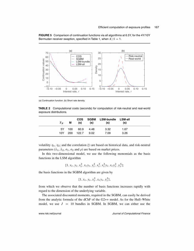
Figure 5(a) compares the reference continuation functions (by COS) with theapproximated continuation functions (by the SGBM and LSM) on the bounded real-ized risk-neutral region at time 6.5Y, for the 4Y/10Y receiver swaption. The approxi-mation by LSM-all is not accurate at the upper and lower regions, which explains itsperformance in Table 1. We observe an accuracy improvement in the results from theLSM-bundle algorithm. From the plot, we observe that the SGBM’s approximatedfunction well resembles the reference value on the whole domain. Figure 5(b) presentsthe empirical density of the risk-neutral short rate and the observed real-world shortrate, where we see that the realized domain under the risk-neutral measure is morewidely spread.

Table 2 gives the computational times for these algorithms. The SGBM is signif-icantly faster than the reference COS algorithm, while the LSM is less accurate butfaster than the SGBM. The experiments are performed on a computer with a CPU IntelCore i7-2600 3.40GHz� 8 processor and 15.6 Gigabytes of RAM. The computationalcost increases proportionally with respect to parameter M .



TABLE 1 Bermudan receiver swaption under the Hull–White model.

(a) 1Y�5Y

K=S Value COS SGBM LSM-bundle LSM-all

40% V0 4.126 4.127(0.00) 4.126(0.01) 4.126(0.01)MPFE 9.125(0.06) 9.118(0.06) 9.039(0.05) 8.8(0.05)EPE 1.704(0.00) 1.705(0.00) 1.708(0.01) 1.806(0.01)100CVA 15.87(0.01) 15.74(0.01) 15.75(0.08) 15.87(0.08)

100% V0 5.463 5.464(0.00) 5.461(0.01) 5.461(0.01)MPFE 11.07(0.05) 11.07(0.05) 11.06(0.05) 10.9(0.04)EPE 2.094(0.00) 2.096(0.00) 2.098(0.00) 2.215(0.00)100CVA 18.56(0.02) 18.33(0.02) 18.35(0.04) 18.44(0.04)

160% V0 7.11 7.11(0.00) 7.113(0.01) 7.113(0.01)MPFE 14.43(0.04) 14.42(0.04) 14.26(0.04) 13.92(0.04)EPE 2.368(0.00) 2.369(0.00) 2.372(0.01) 2.483(0.01)100CVA 21.28(0.02) 20.95(0.02) 20.98(0.05) 21.01(0.05)

(b) 4Y�10Y

K=S Value COS SGBM LSM-bundle LSM-all

40% V0 4.235 4.236(0.00) 4.237(0.01) 4.237(0.01)MPFE 14.12(0.12) 14.13(0.12) 13.86(0.11) 13.16(0.09)EPE 1.827(0.00) 1.829(0.00) 1.834(0.01) 1.91(0.01)100CVA 38.22(0.02) 37.98(0.02) 38.04(0.13) 38.34(0.13)

100% V0 6.199 6.199(0.00) 6.201(0.02) 6.201(0.02)MPFE 19.29(0.11) 19.29(0.11) 19.08(0.12) 18.08(0.10)EPE 2.606(0.00) 2.607(0.00) 2.616(0.01) 2.719(0.01)100CVA 53.35(0.05) 52.92(0.05) 53.03(0.14) 53.26(0.14)

160% V0 8.691 8.691(0.00) 8.687(0.02) 8.687(0.02)MPFE 24.33(0.09) 24.34(0.09) 24.28(0.09) 23.42(0.09)EPE 3.526(0.00) 3.527(0.00) 3.539(0.01) 3.628(0.01)100CVA 71.94(0.06) 71.35(0.06) 71.47(0.09) 71.5(0.10)

(a) S � 0.0109; risk-neutral: � D 0.010, � D 0.020; real-world: � D 0.010, � D 0.015. (b) S � 0.0113; risk-neutral: � D 0.020, � D 0.012; real-world: � D 0.006, � D 0.008. Risk-neutral and real-world scenarios aregenerated; the forward rate is flat, f M.0; t/ D 0.01; the default probability function PS.t/ D 1 � exp.�0.02t/ andLGD D 1; option values and CVA are based on Kq D 100� 103 risk-neutral scenarios; MPFE and EPE are basedon Ka D 100 � 103 real-world scenarios; the number of monitoring dates M D TN =�t with �t D 0.05; standarderrors are in parentheses, based on ten independent runs.

5.2 Experiments with the G2++ model

The dynamics of the risk-neutral and real-world G2++ models are given inAppendix 2(available online), where the associated parameters (ie, the reversion speed �1, �2; the


166 Q. Feng et al

FIGURE 3 Comparison of the mean and 99% quantile of the exposure distributions,computed by the COS method and based on risk-neutral and real-world scenarios, for the4Y/10Y Bermudan receiver swaption, as specified in Table 1, when K=S D 1.

Time0 2 4 6 8 10

EE

0

1

2

3

4

5

6

7

Time0 2 4 6 8 10

PF

E0

5

10

15

20

25

30

35

COS-real-worldCOS-risk-neutral

(a) (b)

(a) Exposure average. (b) Exposure quantile 99%.

FIGURE 4 Comparison of PFE curves obtained by the COS method, SGBM and LSM for2Y–4Y and 6Y–8Y, for the 4Y/10Y Bermudan receiver swaption specified in Table 1, whenK=S D 1.

Time2.0 2.5 3.0 3.5 4.0

PF

E

14

15

16

17

18

19

20

Time6.0 6.5 7.0 7.5 8.0

PF

E

2.0

2.5

3.0

3.5

4.0

4.5

5.0

5.5

COSSGBMLSM-bundleLSM-all

(a) (b)

(a) PFE, 2Y–4Y. (b) PFE, 6Y–8Y.



FIGURE 5 Comparison of continuation functions via all algorithms at 6.5Y, for the 4Y/10YBermudan receiver swaption, specified in Table 1, when K=S D 1.

Interest rate, r–0.10 –0.05 0 0.05 0.10 0.15

Interest rate, r–0.10 –0.05 0 0.05 0.10 0.15

Con

tinua

tion

valu

es

–10

0

10

20

30

40

50

60

70COSSGBMLSM-bundleLSM-all

Den

sity

0

5

10

15

20

25

30Risk-neutralReal-world

(a) (b)

(a) Continuation function. (b) Short rate density.

TABLE 2 Computational costs (seconds) for computation of risk-neutral and real-worldexposure distributions.

COS SGBM LSM-bundle LSM-allTN M (s) (s) (s) (s)

5Y 100 60.9 4.48 3.32 1.6710Y 200 122.7 9.02 7.09 3.26

volatility �1, �2; and the correlation ) are based on historical data, and risk-neutralparameters (1, 2, �1, �2 and �) are based on market prices.

In this two-dimensional model, we use the following monomials as the basisfunctions in the LSM algorithm

f1; xt ; yt ; x2t ; xtyt ; y

2t ; x

3t ; x

2t yt ; xty

2t ; y

3t gI

the basis functions in the SGBM algorithm are given by

f1; xt ; yt ; x2t ; xtyt ; y

2t g;

from which we observe that the number of basis functions increases rapidly withregard to the dimension of the underlying variable.

The associated discounted moments, required in the SGBM, can easily be derivedfrom the analytic formula of the dChF of the G2++ model. As for the Hull–Whitemodel, we use J D 10 bundles in SGBM. In SGBM, we can either use the


168 Q. Feng et al

TABLE 3 Receiver Bermudan swaption under the G2++ model.

(a) 1Y�5Y

K=S Value SGBM LSM-bundle Difference

40% V0 1.742(0.00) 1.747(0.01) 0.005MPFE 5.066(0.02) 5.037(0.17) �0.029EPE 0.771(0.00) 0.773(0.00) 0.002100CVA 7.491(0.01) 7.51(0.03) 0.019

100% V0 2.897(0.00) 2.900(0.01) 0.003MPFE 6.535(0.04) 6.448(0.11) �0.087EPE 1.113(0.00) 1.113(0.01) 0.000100CVA 10.05(0.01) 10.07(0.03) 0.02

160% V0 4.560(0.00) 4.563(0.01) 0.003MPFE 9.652(0.01) 9.601(0.09) �0.51EPE 1.33(0.00) 1.337(0.01) 0.007100CVA 12.67(0.01) 12.7(0.04) 0.03

(b) 3Y�10Y

K=S Value SGBM LSM-bundle Difference

40% V0 0.861(0.00) 0.865(0.00) 0.005MPFE 2.784(0.03) 2.704(0.04) �0.08EPE 0.446(0.00) 0.447(0.00) 0.001100CVA 8.678(0.01) 8.705(0.03) 0.027

100% V0 2.466(0.00) 2.475(0.01) 0.008MPFE 7.176(0.03) 7.115(0.03) �0.061EPE 1.059(0.00) 1.063(0.00) 0.004100CVA 19.53(0.01) 19.61(0.04) 0.08

160% V0 5.42(0.00) 5.428(0.00) 0.008MPFE 12.1(0.03) 12.22(0.04) 0.012EPE 1.839(0.00) 1.846(0.00) 0.007100CVA 35.49(0.01) 35.62(0.04) 0.13

(a) S � 0.0104; risk-neutral: �1 D 0.015, �2 D 0.008, �1 D 0.07, �2 D 0.08, � D �0.6; real-world: �1 D 0.005,�2 D 0.01, �1 D 0.54, �2 D 0.07, D �0.8. (b) S � 0.0102; risk-neutral: �1 D 0.005, �2 D 0.008, �1 D 0.09,�2 D 0.15, � D �0.6; real-world: �1 D 0.002, �2 D 0.006, �1 D 0.04, �2 D 0.07, D �0.8. Risk-neutral and real-world scenarios are generated; forward ratef M.0; t/ D 0.01; the default probability function PS.t/ D 1�exp.�0.02t/and LGD D 1; option values and CVA are based on Kq D 100 � 103 risk-neutral scenarios; MPFE and EPE arebased on Ka D 100� 103 real-world scenarios; the number of monitoring dates M D TN =�t with �t D 0.05.

two-dimensional equal-number bundling method, introduced in Feng and Ooster-lee (2014), or the one-dimensional version based on projecting the high-dimensionalvariable onto a one-dimensional variable. Here, we create the bundles based on therealized values of .xt C yt / on each path at time tm.



FIGURE 6 PFE and the 99% quantile of the exposure distributions of a receiver Bermudanswaption, as specified in Table 3, when K=S D 1.

Time0 2 4 6 8 10

Exp

osur

e

0

2

4

6

8

10

12

Real-world-PFE SGBMReal-world-PFE LSMRisk-neutral 99%-quantile SGBMRisk-neutral 99%-quantile LSM

TABLE 4 Computational costs (seconds) for the computation of risk-neutral and real-worldexposure distributions under the G2++ model.

LSM-bundle SGBMTN M (s) (s)

5Y 100 6.28 8.1010Y 200 12.96 15.07

Table 3 reports the time-zero option value results for SGBM and LSM as well asthe exposure measures for receiver Bermudan swaptions, where we can analyze thedifference between the results by these algorithms.

Figure 6 presents the PFE curves computed on the real-world scenarios as wellas the mean and 99% quantiles of the risk-neutral exposure distributions at eachmonitoring date. As expected, there is a clear difference between the statistics of therisk-neutral and real-world exposure distributions.

Table 4 presents the computational cost of the algorithms for this two-dimensionalmodel. The cost increases with respect to the dimension of the variable.


170 Q. Feng et al

6 CONCLUSION

This paper presents computationally efficient techniques for the simultaneous com-putation of exposure distributions under the risk-neutral and observed real-worldprobability measures. They are based on only two sets of scenarios, one generatedunder the risk-neutral dynamics and another under the observed real-world dynam-ics, as well as on basic techniques such as regression. Compared with nested MonteCarlo simulation, the techniques presented significantly reduce the computationalcost and maintain high accuracy, which we demonstrated by using numerical resultsfor Bermudan swaptions and comparing these with reference results generated by theFourier-based COS method. We illustrated the ease of implementation for both theone-factor Hull–White and two-factor G2++ models.

We recommend the SGBM because of its accuracy and efficiency in the computationof continuation values. A highly satisfactory alternative is to use the LSM-bundleapproach. The reference COS method is highly efficient for computing time-zerovalues of the Bermudan swaption, but for the computation of exposure, there is roomfor improvement in terms of computational speed.

The results for the parameter values chosen show that there are clear differencesin exposure distributions for the risk-neutral and real-world scenarios. The pro-posed algorithms are based on the requirement that the sample space induced bythe observed historical model is a subspace of the sample space under the risk-neutralmeasure.

The valuation framework presented is flexible and may be used efficiently forany type of Bermudan-style claim, such as Bermudan options and swaptions. For aBermudan option, one can compute the sensitivities of CVA at the same time as usingthe SGBM, which is an additional benefit. The algorithms developed can be extendedeasily to the situation in which model parameters are piecewise constant over the timehorizon.

DECLARATION OF INTEREST

The authors report no conflicts of interest. The authors alone are responsible for thecontents of the paper. The views expressed in this paper are those of the authors anddo not necessarily reflect the position of their employers. Financial support from theDutch Technology Foundation STW (project 12214) is gratefully acknowledged.

REFERENCES

Andersen, L. B. (1999). A simple approach to the pricing of Bermudan swaptions in themultifactor Libor market model.The Journal of Computational Finance 3(2), 5–32 (http://doi.org/bkn9).



Andersen, L.B., and Piterbarg,V.V. (2010). Interest Rate Modeling.Atlantic Financial Press.Basel Committee on Banking Supervision (2005). Annex 4 to “International convergence

of capital measurement and capital standards: a revised framework”. Report, Bank forInternational Settlements.

Basel Committee on Banking Supervision (2010). Basel III: a global regulatory frameworkfor more resilient banks and banking systems.Report, Bank for International Settlements.

Brigo, D., and Mercurio, F. (2007). Interest Rate Models – Theory and Practice: With Smile,Inflation and Credit. Springer Science & Business Media.

Fang, F., and Oosterlee, C. W. (2009). Pricing early-exercise and discrete barrier optionsby Fourier-cosine series expansions. Numerische Mathematik 114(1), 27–62 (http://doi.org/b2vhnx).

Feng, Q., and Oosterlee, C. W. (2014). Monte Carlo calculation of exposure profiles andGreeks for Bermudan and barrier options under the Heston Hull–White Model. SSRNWorking Paper, arXiv:1412.3623.

Glasserman, P.(2003).Monte Carlo Methods in Financial Engineering,Volume 53.SpringerScience & Business Media (http://doi.org/bf7w).

Gregory, J. (2010). Counterparty Credit Risk: The New Challenge for Global FinancialMarkets, Volume 470. Wiley.

Hull, J. C., Sokol, A., and White, A. (2014). Modeling the short rate: the real and risk-neutralworlds. Working Paper 2403067, Rotman School of Management (http://doi.org/bkpb).

Jain, S., and Oosterlee, C. W. (2012). Pricing high-dimensional Bermudan options usingthe stochastic grid method. International Journal of Computer Mathematics 89(9), 1186–1211 (http://doi.org/bkpc).

Jain, S., and Oosterlee, C.W. (2015).The stochastic grid bundling method: efficient pricingof Bermudan options and their Greeks. Applied Mathematics and Computation 269,412–431 (http://doi.org/bkpd).

Joshi, M. S., and Kwon, O. K. (2016). Least squares Monte Carlo credit value adjustmentwith small and unidirectional bias. SSRN Working Paper 2717250 (http://doi.org/bkpf).

Karlsson, P., Jain, S., and Oosterlee, C. W. (2014). Counterparty credit exposures forinterest rate derivatives using the stochastic grid bundling method. SSRN WorkingPaper 2538173 (http://doi.org/bkpg).

Kenyon, C., Green, A. D., and Berrahoui, M. (2015). Which measure for PFE? The riskappetite measure A. SSRN Working Paper, December 15, arXiv:1512.06247.

Leitao, Á., and Oosterlee, C. W. (2015). GPU acceleration of the stochastic grid bundlingmethod for early-exercise options. International Journal of Computer Mathematics92(12), 2433–2454 (http://doi.org/bkph).

Longstaff, F. A., and Schwartz, E. S. (2001). Valuing American options by simulation:a simple least-squares approach. Review of Financial Studies 14(1), 113–147 (http://doi.org/b38b5q).

Øksendal, B. (2003). Stochastic Differential Equations. Springer (http://doi.org/dqpdqb).Ruijter, M.J., and Oosterlee, C.W.(2012).Two-dimensional Fourier cosine series expansion

method for pricing financial options. SIAM Journal on Scientific Computing 34(5), B642–B671 (http://doi.org/bkpj).

Ruiz, I. (2012). Backtesting counterparty risk: how good is your model? Technical Report,iRuiz Consulting.


172 Q. Feng et al

Stein, H. J. (2013). Joining risks and rewards. SSRN Working Paper 2368905.Stein, H.J. (2014).Fixing underexposed snapshots:proper computation of credit exposures

under the real world and risk neutral measures. SSRN Working Paper 2365540 (http://doi.org/bkpk).

Zhu, S. H., and Pykhtin, M. (2007). A guide to modeling counterparty credit risk. GARPRisk Review July/August(37), 16–22.


Documents

Research Paper Efﬁcient computation of exposure proﬁles … · 2017-01-16 · and the percentage of loss given default ... portfolio to mitigate the credit risk that arises from