RESEARCH OpenAccess … · RESEARCH OpenAccess Anautomatedtoolforlocalizationofheart soundcomponentsS1,S2,S3andS4in ... and Heron’s formula ... his book, Metrica. The proof of Heron’s

a SpringerOpen Journal

Mondal et al. SpringerPlus 2013, 2:512http://www.springerplus.com/content/2/1/512

RESEARCH Open Access

An automated tool for localization of heartsound components S1, S2, S3 and S4 inpulmonary sounds using Hilbert transform andHeron’s formulaAshok Mondal1*, Parthasarathi Bhattacharya2 and Goutam Saha1

Abstract

The primary problem with lung sound (LS) analysis is the interference of heart sound (HS) which tends to maskimportant LS features. The effect of heart sound is more at medium and high flow rate than that of low flow rate.Moreover, pathological HS obscures LS in a higher degree than normal HS. To get over this problem, several HSreduction techniques have been developed. An important preprocessing step in HS reduction is localization of HScomponents. In this paper, a new HS localization algorithm is proposed which is based on Hilbert transform (HT) andHeron’s formula. In the proposed method, the HS included segment is differentiated from the HS excluded segmentby comparing their area with an adaptive threshold. The area of a HS component is calculated from the Hilbertenvelope using Heron’s triangular formula. The method is tested on real recorded and simulated HS corrupted LSsignals. All the experiments are conducted under low, medium and high breathing flow rates. The proposed methodshows a better performance than the comparative Singular Spectrum Analysis (SSA) based method in terms ofaccuracy (ACC), detection error rate (DER), false negative rate (FNR), and execution time (ET).

Keywords: Filtering; Heart sound localization; Hilbert transform; Heron’s formula; Lung sound

IntroductionThe conventional stethoscope based auscultation tech-nique is a cost-effective and non-invasive diagnosticprocedure. This technique is very popular among thephysicians and commonly used by them since 1816(Laennec 1962). However, the performance of this diag-nostic technique degrades due to the presence of noisein lung sound signals. Modern electronic stethoscope canreduce the ambient noises from lung sounds, but they areinefficient to avoid heart sound noise.During the recording of lung sound, heart sound inter-

feres and changes the temporal and spectral contents ofthe respiratory sound. This may lead to misinterpretationof the underlying lung diseases. Heart sounds compriseof two primary sounds S1 and S2. In addition, it may

*Correspondence: [email protected] of Electronics and Electrical Communication Engineering, IndianInstitute of Technology, Kharagpur, Kharagpur-721 302, IndiaFull list of author information is available at the end of the article

have components like S3, S4 and murmurs associatedwith pathological conditions. The first heart sound, S1and second heart sound, S2 are produced by the openingsof the atrioventricular valves and closures of semilunarvalves, respectively and vice versa (Pourazad 2004). Thethird (S3) HS occurs at the end of S2 due to the vibra-tion of blood inside the ventricles and the fourth (S4) HSis appeared just before the S1 due to the contraction ofatria (Webster 1998; Balasubramaniam and Nedumaran2010). These components carry important informationregarding the cardiac system and are segmented to diag-nose the valvular heart diseases (Schmidt et al. 2010; Tanget al. 2012; Sanei et al. 2011; Patidar and Pachori 2013).However, lung sounds are produced by stochastic and dis-ruptive flow of air within lung airways (Blake 1986). Mostof the heart sound information lies in the frequency rangeof 20-150 Hz (Arnott et al. 1984; Lu et al. 1988; Cromwellet al. 2002) but murmur sounds have a higher frequencyrange of 600 Hz (Patidar and Pachori 2013). On the other

© 2013 Mondal et al.; licensee Springer. This is an Open Access article distributed under the terms of the Creative CommonsAttribution License (http://creativecommons.org/licenses/by/2.0), which permits unrestricted use, distribution, and reproductionin any medium, provided the original work is properly cited.

Mondal et al. SpringerPlus 2013, 2:512 Page 2 of 14http://www.springerplus.com/content/2/1/512

hand, lung sound information spread out over a widerange of frequency approximately 20-1600 Hz (Gavrielyet al. 1981). However, a major part of the lung soundinformation is confined to a frequency less than 200 Hz(Sovijarvi et al. 2000).With the advances in modern technologies, computer

science, and statistical signal processing, a lot of researchwork has been conducted to overcome the problem ofHS removal to highlight the LS (Iyer et al. 1986; Luet al. 1988; Kompis and Russi 1992; Hadjileontiadis andPanas 1997; Gnitecki et al. 2003; Gnitecki and Moussavi2003; Ahlstrom et al. 2005; Yadollahi and Moussavi 2006;Pourazad et al. 2006; Flores-Tapia et al. 2007; Ghaderiet al. 2011). This is an important preprocessing step inlung sound analysis. A common approach of heart soundreduction is high pass filtering of lung sounds. However,this approach attenuates the lung sound components thatresemble to heart sound in spectral domain (Donoho1995). Except the wavelet de-noising technique, the per-formance of all the other heart sound cancellation meth-ods depends on a properly defined heart sound location.Many research groups have developed methods to detectthe heart sounds locations in LS signals. These meth-ods are based on adaptive filtering (Iyer et al. 1986; Luet al. 1988; Kompis and Russi 1992; Hadjileontiadis andPanas 1997; Gnitecki et al. 2003), time-frequency filtering(Pourazad et al. 2006), multiscale product based (Flores-Tapia et al. 2007), and statistical signal analysis (Gniteckiand Moussavi 2003; Ahlstrom et al. 2005; Yadollahi andMoussavi 2006; Ghaderi et al. 2011) approaches. Adap-tive filtering techniques need a reference heart soundsignal which is produced either by the noisy lung soundsignal itself or by an external source, e.g., electrocardio-gram (ECG) signal. A combined theory of spectrogramand wavelet transform analysis is proposed to detect theHS components in (Pourazad et al. 2006). A multiscaleproduct based method is implemented in (Flores-Tapiaet al. 2007) to localize the HS segments. Several sta-tistical methods are used to find out the heart soundlocations, such as variance fractal dimension trajectory(Gnitecki and Moussavi 2003), recurrence time statistics(Ahlstrom et al. 2005), entropy (Yadollahi and Moussavi2006), and singular spectrum analysis (SSA) (Ghaderiet al. 2011). Entropy (ENT) and SSA based algorithms givecomparatively better results than other techniques. How-ever, SSA method gives better results than that of ENTmethod in terms of false negative rate, error in localiza-tion and correlation coefficient. Moreover, SSA method ismuch faster than ENT method. Gadheri et al. has shownthe superiority of SSA method over ENT technique in(Ghaderi et al. 2011).All these techniques highlight their performances for

normal lung sound signals at low and medium flow ratebut not at high flow rate.

The objective of this work is to develop an effectiveand efficient algorithm to localize primary heart sounds(S1 and S2) and pathological heart sounds (S3 and S4)components that is applicable to both normal as well asabnormal cases of lung sounds for three different breath-ing flow rates: low, medium and high. In this paper, a novelheart sounds (S1, S2, S3 and S4) localization algorithmis proposed by using Hilbert transform (Johansson 1999;Mertins 1999) and Heron’s formula (Stanojevié 1997) andthe proposed method is referred to as Hilbert HeronAlgorithm (HHA). The HS and non HS segments arediscriminated by investigating the morphological charac-teristics of the cardiac sounds. It has been taken underconsideration that each HS component extends for a cer-tain duration (Khandpur 2003; Schlant and Alexander1994) and defined by two global minima and one max-imum points. The minima points are correspond to thestarting and ending of the HS component and the maxi-mum point is correspond to the highest energy peak of theHS component. By connecting the global extrema pointssome scalene triangles can be drawn and their areas willbe used to identify the HS and non HS segments. Thearea of the triangle can be computed from the envelopesignal using Heron’s formula. The envelope signal is esti-mated from the filtered mixed LS signal using HT. Thedecision regarding the heart sound included segment orheart sound excluded segment is taken by comparing thearea with an adaptive threshold value. The threshold valueis calculated from the variance of the area vector as dis-cussed in Section “Methodology”. The performance of theproposed method is compared with the SSA method byevaluating the results for both cases of simulated mixedlung sound signals (normal and pathological) and realrecorded lung sound signals. The method gives betterperformance than the SSA method in terms of false neg-ative rate, accuracy, detection error rate, and executiontime.The remaining part of this paper is organized as follows.

Section “Theoretical background on Hilbert transformand Heron’s formula” provides theoretical backgroundon the Hilbert transform and Heron’s formula andSection “Methodology” describes in detail the methodol-ogy. The experimental database and certain implementa-tion issues are described in Section “Experimental datasets and implementation issues” and Section “Results anddiscussion” presents the experimental results and dis-cusses the efficiency of the method. The conclusion isgiven in section “Conclusion”.

Theoretical background on Hilbert transform andHeron’s formulaThe Hilbert transformHilbert transform was developed by German scientistDavid Hilbert (Johansson 1999; Mertins 1999) in the


beginning of the 20th century for interpreting the Eulerformula

e jθ = cosθ + jsinθ (1)

where j is an imaginary unit, i.e., j = √−1. The Hilberttransform of a real valued continuous time domain signal,y(t) is defined by

H{y(t)} = yH(s) = 1π

∮ ∞

−∞y(t)t − s

dt (2)

where s is real and H{·} is the Hilbert operator. Here, theintegration has to be carried out according to the Cauchyprinciple value, that is,

∮ ∞

−∞y(t)t − s

dt = limε→0

(

∫ s−ε

−∞+

∫ ∞

s+ε

)y(t)t − s

dt, ε > 0. (3)

However, real world signals are discontinuous in natureand can be expressed as a discrete-time signal. In the dis-crete domain, the envelope of the real discrete signal y[n]is estimated by the discrete Hilbert transform denoted byHd{·}. The discrete Hilbert transform Hd{·} of a sequencey[n] having a finite period R can be computed using itsDiscrete Fourier transform (DFT). The DFT of y[n] isdenoted by Y [m] is calculated by

Y [m]=R−1∑n=0

y[n]Z−nmR , 0 � m � R − 1. (4)

where ZR = ej2πR , m is the discrete frequency and n is the

discrete time. The DFT Y [m] of the discrete time domainsignal y[n] can be expressed as a combination of a real andan imaginary component, i.e.,

Y [m]= YRe[m]+jY Im[k]

The discrete Hilbert transform yDHT [n] = Hd{y[n] } ofy[n] is calculated as

yDHT [n] = 1R

⎛⎜⎜⎜⎜⎜⎜⎜⎜⎜⎜⎜⎜⎜⎜⎝

(R−1)2∑

m=0YRe[m] sin

( 2πmnR

)

+(R−1)

2∑m=0

YIm[m] cos( 2πmn

R)

−R−1∑

m= (R+1)2

YRe[m] sin( 2πmn

R)

−R−1∑

m= (R+1)2

YIm[m] cos( 2πmn

R)

⎞⎟⎟⎟⎟⎟⎟⎟⎟⎟⎟⎟⎟⎟⎟⎠

(5)

yDHT [n] = 1R

⎛⎜⎜⎜⎜⎜⎜⎜⎜⎜⎜⎜⎜⎜⎜⎝

R2 −1∑m=0

YRe[m] sin( 2πmn

R)

+R2 −1∑m=0

YIm[m] cos( 2πmn

R)

−R−1∑

m= R2 +1

YRe[m] sin( 2πmn

R)

−R−1∑

m= R2 +1

YIm[m] cos( 2πmn

R)

⎞⎟⎟⎟⎟⎟⎟⎟⎟⎟⎟⎟⎟⎟⎟⎠

(6)

The equation (5) is applicable when R is even andequation (6) for odd R.

Heron’s formulaHeron was a Greek mathematician and engineer in 10-70AD (Stanojevié 1997). He contributed much in the field ofoptics, mathematics and enginering. But Heron is popu-lar for deriving the formula for computing the area of thetriangle. The formula consists of two steps:Step 1: Compute the semiperimeter h of the triangle

using the lengths of its sides, u, v, and w as

h = u + v + w2

(7)

Step 2: Calculate the area A of the triangle usingsemiperimeter and the lengths of its sides by theequation (8).

A =√

14v2c2

(1 − cos2 θ

)=

√14v2c2

(1 −

(v2+w2−u2

2vw

)2)

=√(

2u2w2+2u2v2+2v2w2−u4−v4−w416

)= √

(h ∗ (h − u) ∗ (h − v) ∗ (h − w))

(8)

where

θ = ∠vw = arccos(v2 + w2 − u2

2vw

)

The detail of the formula is given in proposition 1.8 ofhis book, Metrica. The proof of Heron’s formula has beendone by Roger Boscovich and stated in (Stanojevié 1997).

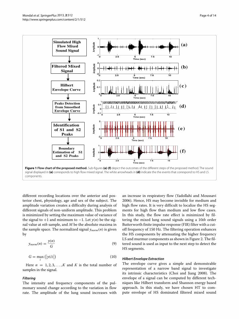
MethodologyThe proposed method distinguishes HS element fromnon HS element based on the principle that heart soundcomponent has higher area than that of the non heartsound component. A flow chart of the proposed methodis given in Figure 1. The entire process is comprised of thefollowing steps:

Amplitude normalizationThe amplitude of the mixed signal varies considerablydue to various factors such as recording instrument gain,


Simulated HighFlow Mixed

Sound Signal

Filtered MixedSignal

HilbertEnvelope Curve

Peaks Detectionfrom SmoothedEnvelope Curve

(a)

(b)

( c )

(d)

Identificationof S1 and S2

Peaks( e )

BoundaryEstimation of S1

and S2 Peaks ( f )

Figure 1 Flow chart of the proposedmethod. Sub-figures (a)-(f) depict the outcomes of the different steps of the proposed method. The soundsignal displayed in (a) corresponds to high flow mixed signal. The white arrowheads in (d) indicate the the events that correspond to HS and LScomponents.

different recording locations over the anterior and pos-terior chest, physiology, age and sex of the subject. Theamplitude variation creates a difficulty during analysis ofdifferent signals of non-uniform amplitude. This problemis minimized by setting the maximum value of variance ofthe signal to +1 and minimum to −1. Let y(n) be the sig-nal value at nth sample, andM be the absolute maxima inthe sample space. The normalized signal ynorm(n) is givenby

ynorm(n) = y(n)

G(9)

G = maxi

(∣∣y(i)∣∣) (10)

Here n = 1, 2, 3, . . . ,K and K is the total number ofsamples in the signal.

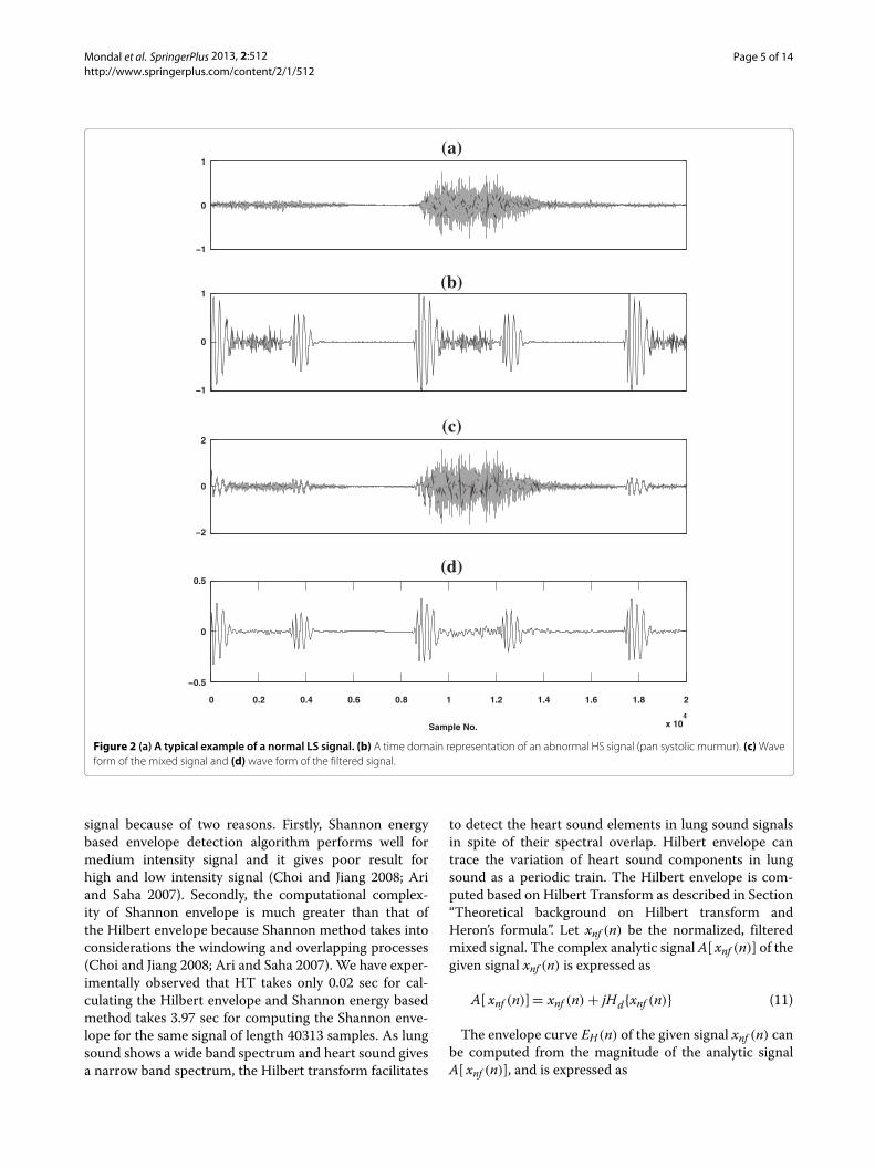
FilteringThe intensity and frequency components of the pul-monary sound change according to the variation in flowrate. The amplitude of the lung sound increases with

an increase in respiratory flow (Yadollahi and Moussavi2006). Hence, HS may become invisible for medium andhigh flow rates. It is very difficult to localize the HS seg-ments for high flow than medium and low flow cases.In this study, the flow rate effect is minimized by fil-tering the mixed lung sound signals using a 10th orderButterworth finite impulse response (FIR) filter with a cut-off frequency of 150 Hz. The filtering operation enhancesthe HS components by attenuating the higher frequencyLS andmurmur components as shown in Figure 2. The fil-tered sound is used as input to the next step to detect theHS segments.

Hilbert Envelope ExtractionThe envelope curve gives a simple and demonstrablerepresentation of a narrow band signal to investigateits intrinsic characteristics (Choi and Jiang 2008). Theenvelope of a signal can be computed by different tech-niques like Hilbert transform and Shannon energy basedapproach. In this study, we have chosen HT to com-pute envelope of HS dominated filtered mixed sound


−1

0

1(a)

−1

0

1(b)

−2

0

2(c)

0 0.2 0.4 0.6 0.8 1 1.2 1.4 1.6 1.8 2

x 104

−0.5

0

0.5

Sample No.

(d)

Figure 2 (a) A typical example of a normal LS signal. (b) A time domain representation of an abnormal HS signal (pan systolic murmur). (c)Waveform of the mixed signal and (d) wave form of the filtered signal.

signal because of two reasons. Firstly, Shannon energybased envelope detection algorithm performs well formedium intensity signal and it gives poor result forhigh and low intensity signal (Choi and Jiang 2008; Ariand Saha 2007). Secondly, the computational complex-ity of Shannon envelope is much greater than that ofthe Hilbert envelope because Shannon method takes intoconsiderations the windowing and overlapping processes(Choi and Jiang 2008; Ari and Saha 2007). We have exper-imentally observed that HT takes only 0.02 sec for cal-culating the Hilbert envelope and Shannon energy basedmethod takes 3.97 sec for computing the Shannon enve-lope for the same signal of length 40313 samples. As lungsound shows a wide band spectrum and heart sound givesa narrow band spectrum, the Hilbert transform facilitates

to detect the heart sound elements in lung sound signalsin spite of their spectral overlap. Hilbert envelope cantrace the variation of heart sound components in lungsound as a periodic train. The Hilbert envelope is com-puted based on Hilbert Transform as described in Section“Theoretical background on Hilbert transform andHeron’s formula”. Let xnf (n) be the normalized, filteredmixed signal. The complex analytic signalA[ xnf (n)] of thegiven signal xnf (n) is expressed as

A[ xnf (n)]= xnf (n) + jHd{xnf (n)} (11)

The envelope curve EH(n) of the given signal xnf (n) canbe computed from the magnitude of the analytic signalA[ xnf (n)], and is expressed as


EH(n) =√xnf (n)2 + Hd{xnf (n)}2 (12)

The phase φ(n) information of the analytic signalA[ xnf (n)] is determined by the following equation

φ(n) = arctan[Hd{xnf (n)

xnf (n)] (13)

Peak Detection in the EnvelopeThe Hilbert envelope curve EH(n) is estimated from thefiltered mixed signal using equation (12) and is shown inFigure 1(c). The envelope signal consists of many peakswhich are originated from the HS components and fromthe low frequency LS components of the filtered mixedsignal as shown in Figure 1(b). Each peak of the envelopecurve EH(n) has a rising and a falling edges, respectively.The rising edge gives the positive gradient values andfalling edge gives negative gradient values at each pointover the envelope. These peaks are detected through thefollowing steps:Step 1: Smoothening of the envelope: The Hilbert enve-

lope EH(n) of the signal is not smooth because of thepresence of lung sound components. Hence, it is requiredto smoothen for more accurate peak detection which isassociated with HS. To accomplish this, a filtering oper-ation is done using a 5th order Butterworth FIR filterwith a cutoff frequency varying in a range of 7-25 Hz.We discuss the effect of variation in cut-off frequency inSection “Results and discussion”.Step 2: Identification of local maxima and minima: The

extreme points of the envelope signal can be calculatedby considering the sign changes across the first derivativeof the envelope. A sample value EH(i) of the smoothedenvelope curve will be a minimum valued point ford(EH (n))

dn |n=i= 0 ‖ d(EH (n−1))dn |n=i< 0 ‖ d(EH (n+1))

dn |n=i> 0and will be a maximum valued point for d(EH (n))

dn |n=i= 0 ‖d(EH (n−1))

dn |n=i> 0 ‖ d(EH (n+1))dn |n=i< 0.

Step 3: Estimation of peaks: A peak consists of threeconsecutive extrema points which include two minimaand one maximum. Each peak has a finite extension fromone minimum point to another as shown in Figure 1(d).The duration of the individual peak varies according to itssource characteristics. The peak locations are identified bycalculating their extreme points and marked with a whitearrow head in Figure 1(d).

Picking up the S1, S2, S3 and S4 peaksThe peaks detected using the above described peak detec-tion framework do not always correspond to heart soundcomponents. Some peaks occur due to the presence ofartifacts and unfiltered lung sound components. The non-heart sound peaks are rejected and the heart sound peaksare selected using a geometrical formula derived by Greekmathematician Heron.

Selection criteria of S1, S2, S3 and S4 peaks: The areaof individual peak is calculated using Heron’s triangularformula. The triangles are formed by connecting theextreme points of the peaks. Let us consider the minimaand maximum points for ith peak are Limin1, Limin2, andLimax, respectively. The length of each side of the triangleassociated with ith peak are calculated as follows:

∣∣ai∣∣ =√[EH(Limax) − EH(Limin 1)]

2

∣∣bi∣∣ =√[EH(Limax) − EH(Limin 2)]

2

∣∣ci∣∣ =√[EH(Limin 2) − EH(Limin 1)]

2

(14)

where ci is the base , ai is the left lateral side and bi is theright lateral side of the triangle. The three angles of thetriangle are defined by the following equation

αi = ∠ai ci = arccos(

(ai)2 + (ci)2 − (bi)2

2ai ci

)

β i = ∠bi ci = arccos(

(bi)2 + (ci)2 − (ai)2

2bi ci

)

γ i = ∠ai bi = arccos(

(ai)2 + (bi)2 − (ci)2

2ai bi

)(15)

where αi, β i and γ i are the angles between the three sides.The lengths of the three sides of the triangle are unequalin magnitude and the angles in between them are alsounequal in degree. Hence this triangle satisfies the crite-rion of scalene triangle. The area �i of the ith triangle iscalculated as

�i =√Si(Si − ai)(Si − bi)(Si − ci) (16)

Si = ai + bi + ci

2(17)

=P∑j=1

Ljmin +Q∑j=1

Ljmax (18)

where i indicates the number of triangle and lies in therange defined by 1 � i � − 2 × Q, P and Q are thetotal number of minima andmaximum points in the enve-lope, respectively. The area of heart sound componentsis higher than that of the artifacts or low frequency lungsound components because heart sound components havea high peak amplitudes as shown in Figure 1(b). The heartsound components S1, S2, S3 and S4 are identified bycomparing the area of the peak with an adaptive thresholdvalue that is calculated from the variance σ of the area vec-tor A =[A1,A2,A3, . . . ,AQ]T , where Ar(r = 1, 2, . . . ,Q)

indicates the area of individual peak in corrupted LS.


The heart sound peaks PHS are selected using theAlgorithm 1.

Algorithm 1 Calculate PHS

Require: Z = Q, σ = 1−2×Q

∑−2×Qm=1 (�m − μ)2,μ =

1−2×Q

∑−2×Qm=1 (�m), j = 1 {σ and μ are the variance

and mean of the area vector A}for k = 1 to Z do

if �k ≥ σ thenPHS(j) ← k

else {�k < σ }PHS(j) ← 0j ← j + 1

end ifend for

Boundary estimation of S1, S2, S3 and S4 peaksThe primary HS components (S1 and S2) extend on bothsides of its peak position as shown in Figure 1(e) for afinite length due to the time gap between the closuresand openings of the heart valves (Pourazad 2004) but thethird (S3) and fourth (S4) HS components extend due tothe relaxation of the ventricle and atrium heart cham-bers (Webster 1998; Balasubramaniam and Nedumaran2010). To estimate the HS boundary, peak location identi-fication is needed. The peak locations are detected usingAlgorithm 1, and after that their boundary BHP are calcu-lated by using Algorithm 2.

Algorithm 2 Calculate BHPRequire: Lmin =[ 1, 2, .....,P] ,NHP = PHS {NHP is the total

number of HS peaks}for p = 1 to NHP do

for q = Lmin(PHS(p)) to Lmin(PHS(p) + 1) doBHP(q) ← 1

end forend for

Experimental data sets and implementation issuesSubjects and data acquisitionThe lung sound signals are recorded from the normal aswell as abnormal male and female subjects using a sin-gle channel stethoscope based data acquisition systemas described in (Mondal et al. 2011). The data acquisi-tion system has been constructed by making a circuitusing active devices (Transistors. Operational Ampli-fiers) and passive elements (Resistors, Capacitors andInductors) fitted to a stethoscope to capture the LS usingthe diaphragm mode. The LS data are recorded from dif-ferent auscultation locations over the body surface (e.g.,

left mid clavicular area, 2nd intercostal and third inter-costal spaces) of the patients in the sitting position andunder relaxing mood conditions. The recordings are notassociated with any particular age group. The recordeddata are arranged in 16 bit, PCM, Mono audio formatand stored as *.wav files at sampling frequency of 8 kHz.The pathological LS are recorded from 8 female and 20male subjects with different types of pulmonary dysfunc-tions: Chronic Obstructive Pulmonary Diseases (COPDs),Interstitial Lung Disease (ILD) and asthma. The patho-logical HS are recorded from 10 female and 22 malesubjects with various valvular heart diseases. On theother hand, the normal LS are recorded from 5 malehealthy subjects and normal HS from 3 female and 5male subjects. The pulmonary sound records are col-lected from various resources: Institute of Pulmocare andResearch, Kolkata, Audio & Biosignal Processing labora-tory, IIT Kharagpur, India and also from R.A.L.E. datasetavailable at:www.rate.cal. The cardiac sound data are col-lected from the two institutes mentioned above and alsofrom the Maulana Azad Medical Institute, Delhi, India.The abnormal lung sounds include wheezes, cracklesand squawks sounds and abnormal heart sounds includelate systolic murmur, pulmonary stenosis, early systolicmurmur, ejection click, aortic insufficiency, pan systolicmurmur, etc.

Synthetic dataThe synthesized mixed lung sound data at different flowrates are generated by a convoluting mixture producingtechnique as described in (Ghaderi et al. 2011). The con-volutive mixtures are simulated by imposing the filteredheart sound components FSHS(t) onto the filtered lungsound components FSLS(t) as given next.

Table 1 The values of norms for different flow rates

TLS THS TM Range of Norm TF

of ap

> 3.10 High

Normal Normal Normal 0.81-3.10 Medium

0.10-0.80 Low

> 3.30 High

Normal Abnormal Abnormal 0.91-3.30 Medium

0.10-0.90 Low

> 3.28 High

Abnormal Normal Abnormal 1.59-3.28 Medium

0.10-1.58 Low

> 3.35 High

Abnormal Abnormal Abnormal 1.97-3.35 Medium

0.10-1.96 Low

TLS: Types of Lung Sounds; THS: Types of Heart Sounds; TM: Types of Mixtures;TF: Type of Flow.

www.rate.cal.


−1

0

1(a)

−1

0

1(b)

−1

0

1(c)

0 0.5 1 1.5 2 2.5 3 3.5 4

x 104

−1

0

1

Sample No.

(d)

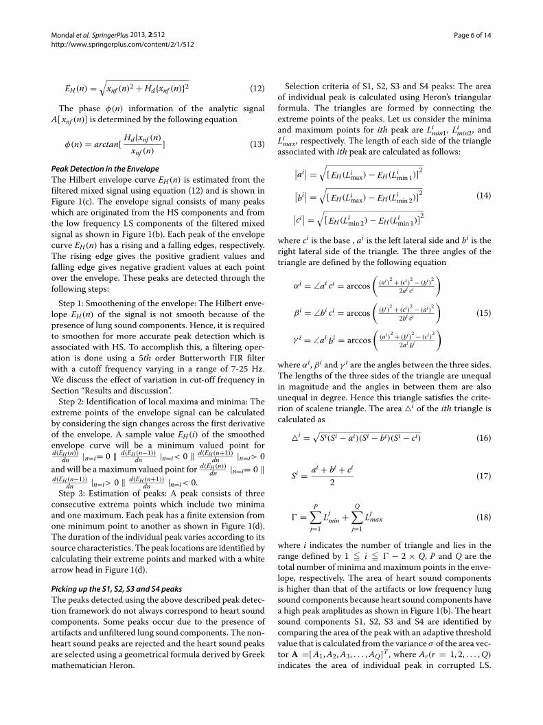
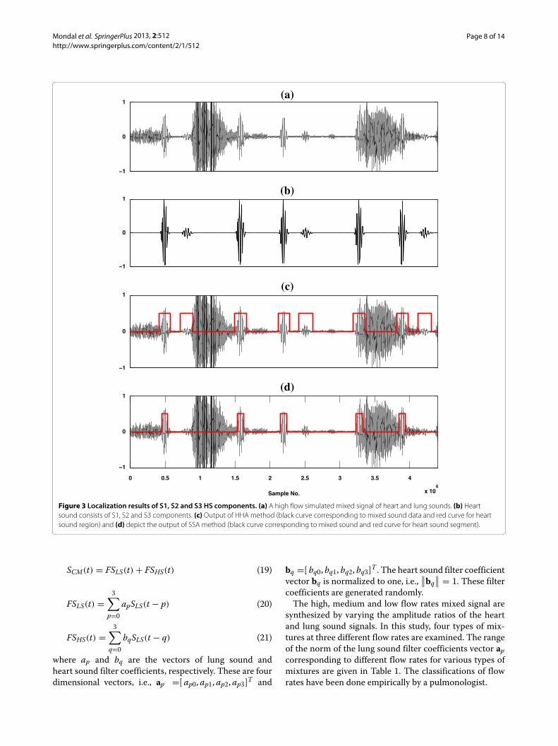
Figure 3 Localization results of S1, S2 and S3 HS components. (a) A high flow simulated mixed signal of heart and lung sounds. (b) Heartsound consists of S1, S2 and S3 components. (c) Output of HHA method (black curve corresponding to mixed sound data and red curve for heartsound region) and (d) depict the output of SSA method (black curve corresponding to mixed sound and red curve for heart sound segment).

SCM(t) = FSLS(t) + FSHS(t) (19)

FSLS(t) =3∑

p=0apSLS(t − p) (20)

FSHS(t) =3∑

q=0bqSLS(t − q) (21)

where ap and bq are the vectors of lung sound andheart sound filter coefficients, respectively. These are fourdimensional vectors, i.e., ap =[ ap0, ap1, ap2, ap3]T and

bq =[ bq0, bq1, bq2, bq3]T . The heart sound filter coefficientvector bq is normalized to one, i.e.,

∥∥bq∥∥ = 1. These filtercoefficients are generated randomly.The high, medium and low flow rates mixed signal are

synthesized by varying the amplitude ratios of the heartand lung sound signals. In this study, four types of mix-tures at three different flow rates are examined. The rangeof the norm of the lung sound filter coefficients vector apcorresponding to different flow rates for various types ofmixtures are given in Table 1. The classifications of flowrates have been done empirically by a pulmonologist.


−1

0

1(a)

−1

0

1(b)

−1

0

1(c)

0 0.5 1 1.5 2 2.5 3 3.5 4

x 104

−1

0

1

Sample No.

(d)

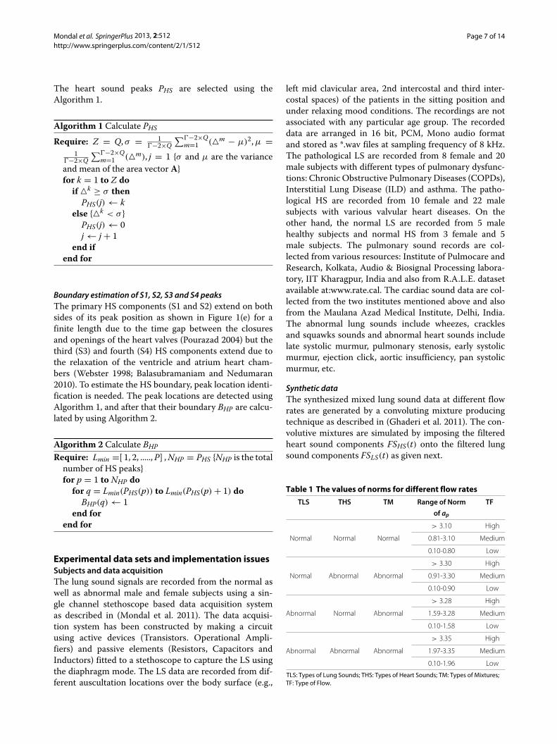
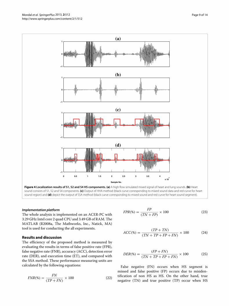
Figure 4 Localization results of S1, S2 and S4 HS components. (a) A high flow simulated mixed signal of heart and lung sounds. (b) Heartsound consists of S1, S2 and S4 components. (c) Output of HHA method (black curve corresponding to mixed sound data and red curve for heartsound region) and (d) depict the output of SSA method (black curve corresponding to mixed sound and red curve for heart sound segment).

Implementation platformThe whole analysis is implemented on an ACER-PC with3.29 GHz Intel core 2 quad CPU and 3.49 GB of RAM. TheMATLAB (R2008a, The Mathworks, Inc., Natick, MA)tool is used for conducting the all experiments.

Results and discussionThe efficiency of the proposed method is measured byevaluating the results in terms of false positive rate (FPR),false negative rate (FNR), accuracy (ACC), detection errorrate (DER), and execution time (ET), and compared withthe SSA method. These performance measuring units arecalculated by the following equations:

FNR(%) = FN(TP + FN)

× 100 (22)

FPR(%) = FP(TN + FP)

× 100 (23)

ACC(%) = (TP + TN)

(TN + TP + FP + FN)× 100 (24)

DER(%) = (FP + FN)

(TN + TP + FP + FN)× 100 (25)

False negative (FN) occurs when HS segment ismissed and false positive (FP) occurs due to misiden-tification of non HS as HS. On the other hand, truenegative (TN) and true positive (TP) occur when HS


−1

0

1(a)

−1

0

1(b)

0 0.5 1 1.5 2 2.5 3 3.5 4

x 104

−1

0

1

Sample No.

(c)

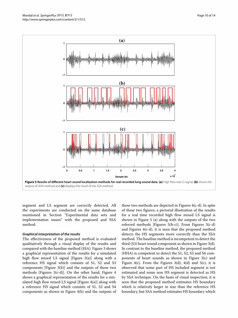
Figure 5 Results of different heart sound localization methods for real recorded lung sound data. (a) High flow real LS signal, (b) shows theoutput of HHA method and (c) displays the result of the SSA method.

segment and LS segment are correctly detected. Allthe experiments are conducted on the same databasementioned in Section “Experimental data sets andimplementation issues” with the proposed and SSAmethod.

Graphical interpretation of the resultsThe effectiveness of the proposed method is evaluatedqualitatively through a visual display of the results andcompared with the baseline method (SSA). Figure 3 showsa graphical representation of the results for a simulatedhigh flow mixed LS signal [Figure 3(a)] along with areference HS signal which consists of S1, S2 and S3components [Figure 3(b)] and the outputs of these twomethods [Figures 3(c-d)]. On the other hand, Figure 4shows a graphical representation of the results for a sim-ulated high flow mixed LS signal [Figure 4(a)] along witha reference HS signal which consists of S1, S2 and S4components as shown in Figure 4(b) and the outputs of

these two methods are depicted in Figures 4(c-d). In spiteof these two figures, a pictorial illustration of the resultsfor a real time recorded high flow mixed LS signal isshown in Figure 5 (a) along with the outputs of the tworeferred methods [Figures 5(b-c)]. From Figures 3(c-d)and Figures 4(c-d), it is seen that the proposed methoddetects the HS segments more correctly than the SSAmethod. The baselinemethod is incompetent to detect thethird (S3) heart sound component as shown in Figure 3(d).In contrast to the baseline method, the proposed method(HHA) is competent to detect the S1, S2, S3 and S4 com-ponents of heart sounds as shown in Figure 3(c) andFigure 4(c). From the Figures 3(d), 4(d) and 5(c), it isobserved that some part of HS included segment is notestimated and some non HS segment is detected as HSby SSA technique. On the basis of visual inspection, it isseen that the proposed method estimates HS boundarywhich is relatively larger in size than the reference HSboundary, but SSA method estimates HS boundary which


Table 2 Performance of the different HS localizationmethods, HHA and SSA for the synthetic mixtures of normal HS andnormal LS at three different flow rates

TF Method Error (%) ACC DER ET

FNR FPR (%) (%) (Sec)

L HHA 0.0 ± 0.0 1.05 ± 0.04 99.15 ± 0.03 0.83 ± 0.03 0.38 ± 0.01

L SSA 24.63 ± 0.18 0.0 ± 0.0 96.05 ± 0.02 3.94 ± 0.02 1.39 ± 0.01

M HHA 0.00 ± 0.0 2.42 ± 0.34 98.00 ± 0.27 1.99 ± 0.27 0.38 ± 0.01

M SSA 28.10 ± 0.18 0.0 ± 0.0 95.49 ± 0.03 4.49 ± 0.03 1.39 ± 0.01

H HHA 0.0 ± 0.0 5.46 ± 0.31 95.63 ± 0.23 4.35 ± 0.23 0.38 ± 0.01

H SSA 34.90 ± 0.14 0.0 ± 0.0 94.40 ± 0.05 5.59 ± 0.05 1.39 ± 0.01

TF: Types of Flows; FNR: False Negative Rate; FPR: False Positive Rate; ACC: Accuracy; DER: Detection Error Rate; ET: Execution Time.

Table 3 Performance of the different HS localizationmethods, HHA and SSA for the synthetic mixtures of normal HS andabnormal LS at three different flow rates



L HHA 0.0 ± 0.0 1.85 ± 0.30 98.46 ± 0.25 1.53 ± 0.25 0.38 ± 0.01

L SSA 25.80 ± 0.49 0.0 ± 0.0 95.86 ± 0.08 4.13 ± 0.08 1.39 ± 0.01

M HHA 0.00 ± 0.0 2.86 ± 0.31 97.49 ± 0.14 2.49 ± 0.14 0.38 ± 0.01

M SSA 31.85 ± 0.07 0.0 ± 0.0 94.88 ± 0.15 5.10 ± 0.15 1.39 ± 0.01

H HHA 0.0 ± 0.0 7.11 ± 0.08 94.41 ± 0.26 5.57 ± 0.26 0.38 ± 0.01

H SSA 37.09 ± 1.94 2.27 ± 1.66 92.11 ± 2.74 7.88 ± 2.74 1.39 ± 0.01


Table 4 Performance of the different HS localizationmethods, HHA and SSA for the synthetic mixtures of abnormal HSand normal LS at three different flow rates



L HHA 0.0 ± 0.0 3.05 ± 0.32 97.92 ± 0.21 2.06 ± 0.21 0.38 ± 0.01

L SSA 25.92 ± 0.59 0.0 ± 0.0 91.06 ± 0.20 8.92 ± 0.20 1.39 ± 0.01

M HHA 0.00 ± 0.0 4.94 ± 0.47 96.73 ± 0.30 3.25 ± 0.30 0.38 ± 0.01

M SSA 32.98 ± 1.76 0.0 ± 0.0 88.63 ± 0.60 11.36 ± 0.60 1.39 ± 0.01

H HHA 0.0 ± 0.0 14.07 ± 1.25 91.57 ± 0.65 8.41 ± 0.65 0.38 ± 0.01

H SSA 44.27 ± 3.30 2.64 ± 1.84 81.38 ± 0.92 18.59 ± 0.92 1.39 ± 0.01


Table 5 Performance of the different HS localizationmethods, HHA and SSA for the synthetic mixtures of abnormal HSand abnormal LS at three different flow rates



L HHA 0.0 ± 0.0 4.43 ± 0.60 97.01 ± 0.30 2.97 ± 0.30 0.38 ± 0.01

L SSA 27.15 ± 1.26 0.0 ± 0.0 90.42 ± 0.47 9.56 ± 0.47 1.39 ± 0.01

M HHA 0.00 ± 0.0 6.81 ± 0.39 95.59 ± 0.23 4.39 ± 0.23 0.38 ± 0.01

M SSA 34.83 ± 0.95 0.83 ± 0.20 87.44 ± 0.25 12.54 ± 0.25 1.39 ± 0.01

H HHA 0.0 ± 0.0 16.37 ± 0.72 90.40 ± 0.35 9.58 ± 0.35 0.38 ± 0.01

H SSA 45.34 ± 0.64 3.97 ± 0.76 79.25 ± 1.69 20.73 ± 1.69 1.39 ± 0.01



Table 6 Performance of the different HS localizationmethods, HHA and SSA for the real time recorded lung sounds atthree different flow rates



L HHA 0.0 ± 0.0 2.50 ± 0.33 98.15 ± 0.21 1.83 ± 0.21 0.23 ± 0.01

L SSA 25.84 ± 0.99 0.69 ± 0.47 95.42 ± 0.78 4.56 ± 0.78 1.45 ± 0.01

M HHA 0.0 ± 0.0 5.83 ± 0.10 95.59 ± 0.33 4.40 ± 0.33 0.23 ± 0.01

M SSA 29.19 ± 0.52 1.24 ± 0.97 92.96 ± 0.87 7.03 ± 0.89 1.45 ± 0.01

H HHA 0.0 ± 0.0 11.66 ± 0.80 93.05 ± 0.59 6.94 ± 0.59 0.23 ± 0.01

H SSA 36.25 ± 0.61 1.53 ± 1.44 90.40 ± 1.68 9.59 ± 1.68 1.45 ± 0.01


is relatively less in size than the reference HS boundary.The performance of the proposed method is measuredby comparing its output HS boundary with the referenceHS boundary. In this study, the boundary of reference HSsignal is calculated by three expert physicians based onauditory test and visual inspection of spectrogram andwaveform of the reference HS signal.

Quantitative evaluation of the resultsA quantitative comparisons of these two methods aregiven in Tables 2, 3, 4, 5, 6. Tables 2, 3, 4, 5, present theresults for normal and pathological simulated data andTable 6 gives results for real recorded data. The FNR,ACC, and DER of the proposed method are significantlybetter than the SSA method for various types of mixture(Tables 2, 3, 4, 5,) and real LS data (Table 6) at different

flow rates. Moreover, the proposed method is faster thanthe SSA method. On the other hand, SSA method is bet-ter in term of FPR. However, the performance of any heartsound reduction technique which follows a preprocessingstep of HS localization, depends on a correct estimationof HS segments. So, it is more important to estimate thesegment that contains HS information than the detectionof non HS segment as HS segment. The FNR value ofSSA method and FPR value of the proposed method aregreater for pathological HS signal than the normal HS sig-nal due to the presence of murmur in cardiac sound signal.The performance of the two methods degrades graduallywith increase of flow rate because of the superimpositionof LS over HS. The SSA method gives a higher valuedFNR for medium and high flow pathological signals. Toovercome these difficulties, two modifications have been

5 10 15 20 25 30 350

10

20

30

40

50

60

Cut off frequency (fc)

FN

R /

FP

R

FPR

FNR

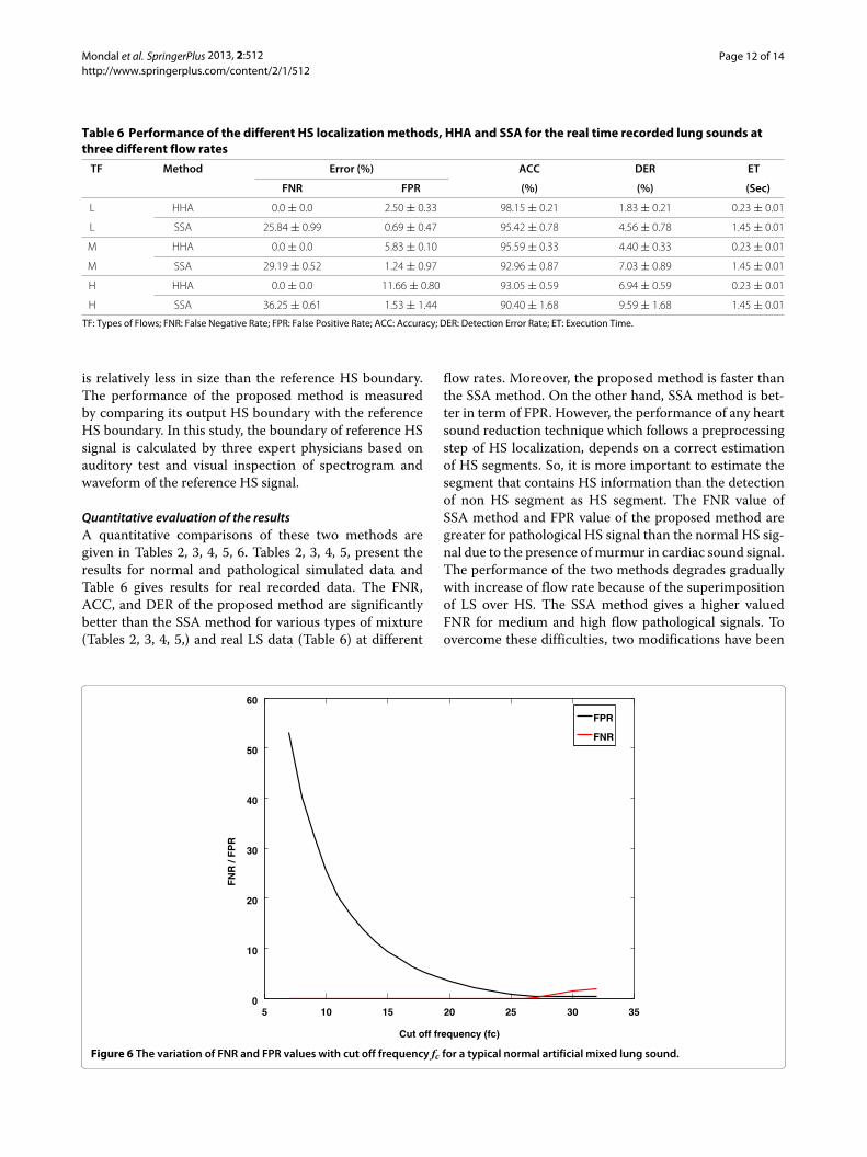
Figure 6 The variation of FNR and FPR values with cut off frequency fc for a typical normal artificial mixed lung sound.


0 500 1000 1500 2000 2500 3000−1.5

−1

−0.5

0

0.5

1

1.5x 10

−3

Sample No.

Mag

nit

ud

e o

f g

rad

ien

t

fc=8Hz

fc=12Hz

fc=16Hz

fc=20Hz

fc=24Hz

fc=28Hz

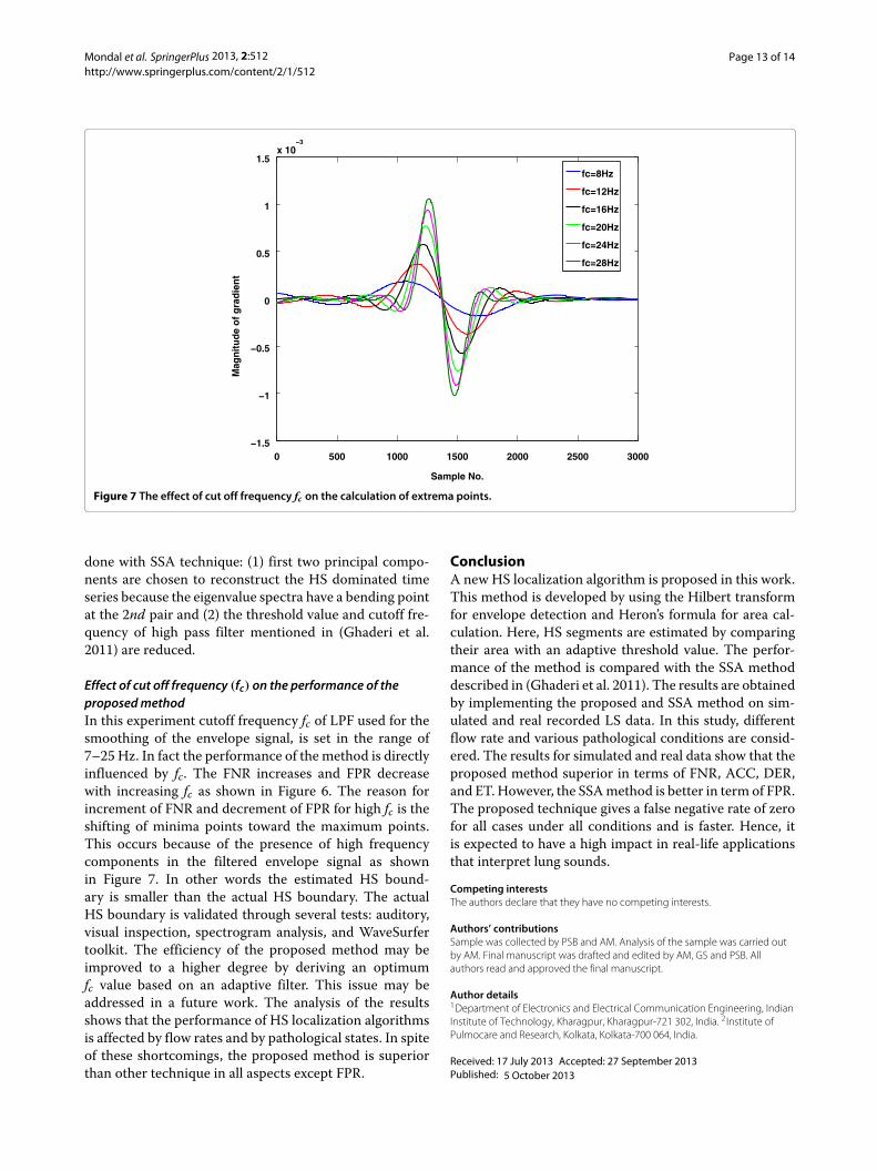
Figure 7 The effect of cut off frequency fc on the calculation of extrema points.

done with SSA technique: (1) first two principal compo-nents are chosen to reconstruct the HS dominated timeseries because the eigenvalue spectra have a bending pointat the 2nd pair and (2) the threshold value and cutoff fre-quency of high pass filter mentioned in (Ghaderi et al.2011) are reduced.

Effect of cut off frequency (fc) on the performance of theproposedmethodIn this experiment cutoff frequency fc of LPF used for thesmoothing of the envelope signal, is set in the range of7–25 Hz. In fact the performance of the method is directlyinfluenced by fc. The FNR increases and FPR decreasewith increasing fc as shown in Figure 6. The reason forincrement of FNR and decrement of FPR for high fc is theshifting of minima points toward the maximum points.This occurs because of the presence of high frequencycomponents in the filtered envelope signal as shownin Figure 7. In other words the estimated HS bound-ary is smaller than the actual HS boundary. The actualHS boundary is validated through several tests: auditory,visual inspection, spectrogram analysis, and WaveSurfertoolkit. The efficiency of the proposed method may beimproved to a higher degree by deriving an optimumfc value based on an adaptive filter. This issue may beaddressed in a future work. The analysis of the resultsshows that the performance of HS localization algorithmsis affected by flow rates and by pathological states. In spiteof these shortcomings, the proposed method is superiorthan other technique in all aspects except FPR.

ConclusionA new HS localization algorithm is proposed in this work.This method is developed by using the Hilbert transformfor envelope detection and Heron’s formula for area cal-culation. Here, HS segments are estimated by comparingtheir area with an adaptive threshold value. The perfor-mance of the method is compared with the SSA methoddescribed in (Ghaderi et al. 2011). The results are obtainedby implementing the proposed and SSA method on sim-ulated and real recorded LS data. In this study, differentflow rate and various pathological conditions are consid-ered. The results for simulated and real data show that theproposed method superior in terms of FNR, ACC, DER,and ET. However, the SSAmethod is better in term of FPR.The proposed technique gives a false negative rate of zerofor all cases under all conditions and is faster. Hence, itis expected to have a high impact in real-life applicationsthat interpret lung sounds.

Competing interestsThe authors declare that they have no competing interests.

Authors’ contributionsSample was collected by PSB and AM. Analysis of the sample was carried outby AM. Final manuscript was drafted and edited by AM, GS and PSB. Allauthors read and approved the final manuscript.

Author details1Department of Electronics and Electrical Communication Engineering, IndianInstitute of Technology, Kharagpur, Kharagpur-721 302, India. 2Institute ofPulmocare and Research, Kolkata, Kolkata-700 064, India.

Received: 17 July 2013 Accepted: 27 September 2013Published: 5 October 2013


ReferencesAhlstrom C, Liljefeldt O, Hult P, Ask P (2005) Heart sound cancellation from

lung sound recordings using recurrence time statistics and nonlinearprediction. Signal Process Lett, IEEE 12(12): 812–815

Ari S, Saha G (2007) On a robust algorithm for heart sound segmentation.JMMB 7(2): 129–150

Arnott P, Pfeiffer G, Tavel M (1984) Spectral analysis of heart sounds:relationships between some physical characteristics and frequency spectraof first and second heart sounds in normals and hypertensives. J BiomedEng 6(2): 121–128

Balasubramaniam D, Nedumaran D (2010) Efficient computation ofphonocardiographic signal analysis in digital signal processor basedsystem. IJCTE 2(4): 660–664

Blake WK (1986) Mechanics of flow-induced sound and vibration. AcademicPress, Orlando, FL

Choi S, Jiang Z (2008) Comparison of envelope extraction algorithms forcardiac sound signal segmentation. Expert Syst Appli 34(2): 1056–1069

Cromwell L, Weibell FJ, Pfeiffer EA (eds) (2002) Biomedical instrumentation andmeasurements. PHI Publication, New Delhi, India

Donoho DL (1995) De-noising by soft-thresholding. IEEE Trans Inf Theory 41(3):613–627

Flores-Tapia D, Moussavi Z, Thomas G (2007) Heart sound cancellation basedon multiscale products and linear prediction. IEEE Trans Biomed Eng 54(2):234–243

Gavriely N, Palti Y, Alroy G (1981) Spectral characteristics of normal breathsounds. J Appl Physiol 50(2): 307–314

Ghaderi F, Mohseni H, Sanei S (2011) Localizing heart sounds in respiratorysignals using singular spectrum analysis. IEEE Trans Biomed Eng 58(12):3360–3367

Gnitecki J, Moussavi Z, Pasterkamp H (2003) Recursive least squares adaptivenoise cancellation filtering for heart sound reduction in lung soundsrecordings. Engineering in medicine and biology society, Proceedings ofthe 25th annual international conference of the IEEE, Cancun, Mexico2416–2419

Gnitecki J, Moussavi Z (2003) Variance fractal dimension trajectory as a tool forheart sound localization in lung sounds recordings. Engineering inmedicine and biology society, Proceedings of the 25th annualinternational conference of the IEEE, Cancun, Mexico 2420–2423

Hadjileontiadis L, Panas S (1997) Adaptive reduction of heart sounds from lungsounds using fourth-order statistics. IEEE Trans Biomed Eng 44(7): 642–648

Iyer VK, Ramamoorthy PA, Fan H, Ploysongsang Y (1986) Reduction of heartsounds from lung sounds by adaptive filtering. IEEE Trans Biomed Eng33(12): 1141–1148

Johansson M (1999) The Hilbert transform. Master thesis, Vaxjo UniversityKhandpur RS (ed) (2003) Handbook of biomedical instrumentation. Tata

McGraw Hill, New Delhi, IndiaKompis M, Russi E (1992) Adaptive heart-noise reduction of lung sounds

recorded by a single microphone. Engineering in medicine and biologysociety, Proceedings of the 14th annual international conference of theIEEE, Paris, France, pp 691–692

Laennec RTH (1962) Invention of the stethoscope. Acoustic historical andphilosophical development. Hutchinson and Ross Inc, Stroudsburg, PA:Dowden

Lu YS, Liu WH, Qin GX (1988) Removal of the heart sound noise from thebreath sound. Engineering in medicine and biology society, Proceedingsof the 25th annual international conference of the IEEE. New Orleans, LA,USA, pp 175–176

Mertins A (1999) Signal analysis; wavelets, filter banks. Wiley, EnglandMondal A, Bhattacharya PS, Saha G (2011) Reduction of heart sound

interference from lung sound signals using empirical modedecomposition technique. JMET 35(6): 344–353

Patidar S, Pachori RB (2013) Segmentation of cardiac sound signals byremoving murmurs using constrained tunable-q wavelet transform.Biomed Signal Proc Control 8(6): 559–567

Pourazad M (2004) Heart sounds reduction from lung sounds recordingsapplying signal and image processing techniques in time-frequencydomain. Master thesis, University of Manitoba

Pourazad M, Moussavi Z, Thomas G (2006) Heart sound cancellation from lungsound recordings using time-frequency filtering. MBEC 44(3): 216–225

Sanei S, Ghodsi M, Hassani H (2011) An adaptive singular spectrum analysisapproach to murmur detection from heart sounds. Med Eng& Physics33(3): 362–367

Schlant RC, Alexander RW (eds) (1994) The heart arteries and veins, Vol. 1.McGraw Hill Inc., Ch. 11 New York, USA

Schmidt S, Holst-Hansen C, Graff C, Toft E, Struijk JJ (2010) Segmentation ofheart sound recordings by a duration-dependent hidden markov model.Physiol Meas 31(4): 513–529

Sovijarvi A, Malmberg L, Charbonneau G, Vanderschoot J, Dalmasso F, Sacco C,Rossi M, Earis J (2000) Characteristics of breath sounds and adventitiousrespiratory sounds. Eur Respir Rev 10(77): 591–596

Stanojevié M (1997) Proof of the Hero’s formula according to R. Boscovich.Math Commun 2(1): 83–88

Tang H, Li T, Qiu T, Park Y (2012) Segmentation of heart sounds based ondynamic clustering. Biomed Signal Proc Control 7(5): 509–516

Webster J (1998) Medical instrumentation: Application and design. John Wiley& Sons, New York

Yadollahi A, Moussavi Z (2006) A robust method for heart sounds localizationusing lung sounds entropy. IEEE Trans Biomed Eng 53(3): 497–502

doi:10.1186/2193-1801-2-512Cite this article as:Mondal et al.:An automated tool for localization of heartsound components S1, S2, S3 and S4 in pulmonary sounds using Hilberttransform and Heron’s formula. SpringerPlus 2013 2:512.

Submit your manuscript to a journal and benefi t from:

7 Convenient online submission

7 Rigorous peer review

7 Immediate publication on acceptance

7 Open access: articles freely available online

7 High visibility within the fi eld

7 Retaining the copyright to your article

Submit your next manuscript at 7 springeropen.com

Documents

RESEARCH OpenAccess … · RESEARCH OpenAccess Anautomatedtoolforlocalizationofheart soundcomponentsS1,S2,S3andS4in ... and Heron’s formula ... his book, Metrica. The proof of Heron’s