Embed Size (px)
Citation preview

Madison et al. Integrating Materials and Manufacturing Innovation 2014, 3:11http://www.immijournal.com/content/3/1/11
RESEARCH Open Access
Advancing quantitative description of porosity inautogenous laser-welds of 304L stainless steelJonathan D Madison1*, Larry K Aagesen2, Victor WL Chan2 and Katsuyo Thornton2
* Correspondence:[email protected] Materials & DataScience, Sandia NationalLaboratories, 87185 Albuquerque,NM, USAFull list of author information isavailable at the end of the article
©Am
Abstract
Porosity in linear autogenous laser welds of 304L stainless steel has beeninvestigated using micro-computed tomography to reveal defect content in fifty-fourwelds made with varying delivered power, travel speed and focal lens. Trends associatedwith porosity size and frequencies are shown and interfacial measures are employedto provide quantitative descriptors of pore shape, directionality, interspacing andsolid linear fraction. Lastly, the coefficient of variation associated with equivalentpore radii is reported toward a discussion of microstructural variability and the influenceof process-parameters on such variability.
Keywords: Micro-computed tomography; Porosity; Stainless steel; Interfacial shapedistribution; Interfacial normal distribution
BackgroundAmong joining and metal processing techniques used in industrial and scientific cap-
acities, laser welding is relatively new. Due to its ability to supply high densities of
power to very controlled areas with minimal peripheral excess heat input, it has be-
come a rapidly growing and highly attractive joining process for metals [1,2]. Common
interrogation practice for welds are often performed via post-mortem failure analysis
[3], post-process radiography [4], or ultrasonic scan [5]. Typically, these evaluations
provide an opportunity to identify the most probable cause of failure, or produce a
qualitative understanding of the internal structure of the weld.
For most engineering metals, there exists a fairly clear inverse correlation between
pore volume and mechanical properties such as strength or modulus with varying de-
grees of sensitivity. As a specific example, defects such as pores, occurring naturally or
imposed artificially, have been shown to serve as preferred sites for the initiation or
propagation of failure in creep in both conventional and high cycle fatigue of
aluminum [6,7], a material system having high formability and broad applications.
304L stainless steel is unique in this regard as the effects of porosity on some material
properties challenge intuition. Two examples in the literature which illustrate this phe-
nomena can be found in the work of Boyce et al. [3] and Kuo and Jeng [8]. In the work
of Boyce et al., autogenous continuous-wave and pulsed-wave laser welds were made
across the gauge section of 304L stainless-steel tensile bars, which were subsequently
strained to failure. While one weld schedule was noted to produce higher amounts of
porosity than the other, no decrease in mechanical strength was observed. In the work
2014 Madison et al.; licensee Springer. This is an Open Access article distributed under the terms of the Creative Commonsttribution License (http://creativecommons.org/licenses/by/2.0), which permits unrestricted use, distribution, and reproduction in anyedium, provided the original work is properly credited.
Madison et al. Integrating Materials and Manufacturing Innovation 2014, 3:11 Page 2 of 17http://www.immijournal.com/content/3/1/11
of Kuo and Jeng, a variety of weld schedules were created for 304L stainless steel,
where increasing porosity levels coincided with decreases in hardness and relatively
small variations in yield strength. Additionally, the continuous-wave-laser weld sample,
which contained higher amounts of porosity than any pulsed-wave-laser weld sample,
demonstrated significantly higher tensile strength than all pulsed-wave-laser weld sam-
ples [8]. These findings suggest that the interplay of processing parameters may affect
laser-welded microstructure in ways that complicate the individual effect of porosity,
particularly in 304L. Furthermore, both examples illustrate that the effects of laser-
welding induced porosity in 304L on certain mechanical properties is not clearly under-
stood. We suggest that advancing the quantitative description of porosity in 304L laser
weldments and relating them directly to carefully controlled weld parameters can assist
in better understanding the concomitant effects of porosity in this ubiquitous and
highly damage-tolerant material system.
Fortunately, for nearly all metallic systems, the parameters used to form the laser-
weld are among the most pivotal factors that determine the local microstructure. Typical
processing parameters may include; shielding gas, laser power, power profile, filler ma-
terial, travel speed and focal distance between the laser source and weld surface. The
combination of these factors is often referred to as the ‘weld schedule’. In this study,
parameters of the weld schedule investigated have been limited to weld power, travel
speed and focal length. Fortunately, recent advances in characterization and micro-
structure visualization have provided a rich set of tools being increasingly brought to
bear on laser-weld induced porosity in a variety of metals [9-13]. The work presented
here builds upon such investigations and utilizes micro-computed tomography and
other emerging state-of-the-art three-dimensional (3D) characterization techniques to
quantitatively relate porosity in autogenous laser-welds of 304L stainless-steel to spe-
cific processing parameters [9,10,14].
MethodsUsing a ROFIN-Sinar, Inc. CW 0.15 HQ, fiber-optic delivered Nd:YAG laser, over fifty
unique weld-schedules were used to produce autogenous standing-edge seam welds in
304L stainless steel having an elemental composition of Fe–0.04C–18.12Cr–1.21Mn–
8.09Ni–0.028 N–0.022P–0.001S–0.34Si (wt.%). In all subsequent depictions, the x-direc-
tion denotes the weld width, the z-direction denotes the weld length and the y-direction
denotes the weld depth, which is also the axis of incidence of the laser relative to the sam-
ple. For each sample, a standing-edge weld was formed by affixing two 2.54 cm×
10.16 cm× 0.1 cm flat plates together face-to-face by base-clamp, then laser-welding their
upper seam at one of five constant travel speeds (254 mm×min−1, 508 mm×min−1,
1016 mm×min−1, 1524 mm×min−1 or 2032 mm×min−1) and at one of six delivered
powers ranging from 200 W to 1200 W as measured with a Macken P2000Y laser
power-probe. This parameter set included a total of 27 separate weld schedules and
was performed for two separate focal lengths, 80 mm and 120 mm, bringing the total
weld schedule count to 54. For a complete matrix of the weld schedules investigated,
see Table 1.
Following welding, micro-computed tomography (μCT) was performed on each sam-
ple to reveal the size, location and morphology of the internal porosity. A Kevex PSX
10-65 W x-ray tube was employed using a 250 μA current and 130 kV operating

Table 1 Maximum pore volume and total pores observed per case
80 mm lens
252mm×min−1 510mm×min−1 1016mm×min−1 1524mm×min−1 2032mm×min−1
1200 W 0.49 mm3 (373) 0.05 mm3 (550) 0.03 mm3 (425)
1000 W 0.76 mm3 (160) 0.30 mm3 (337) 0.03 mm3 (603) 0.02 mm3 (403)
800 W 0.28 mm3 (60) 0.79 mm3 (190) 0.1 mm3 (612) 0.03 mm3 (835) 0.016 mm3 (349)
600 W 0.17 mm3 (145) 0.38 mm3 (247) 0.045 mm3 (652) 0.013 mm3 (406) 0.008 mm3 (192)
400 W 0.08 mm3 (394) 0.02 mm3 (343) 0.009 mm3 (116) 0.0005 mm3 (10) 0.0007 mm3 (20)
200 W – (0) – (0) – (0) – (0) – (0)
120 mm lens
252mm×min−1 510mm×min−1 1016mm×min−1 1524mm×min−1 2032mm×min−1
1200 W 0.95 mm3 (431) 0.10 mm3 (391) 0.03 mm3 (736)
1000 W 1.50 mm3 (130) 0.51 mm3 (190) 0.57 mm3 (381) 0.01 mm3 (263)
800 W 0.17 mm3 (77) 0.59 mm3 (129) 0.09 mm3 (302) 0.01 mm3 (290) 0.006 mm3 (264)
600 W 0.24 mm3 (120) 0.26 mm3 (284) 0.01 mm3 (267) 0.007 mm3 (132) 0.009 mm3 (91)
400 W 0.07 mm3 (81) 0.01 mm3 (6) 0.001 mm3 (1) – (0) – (0)
200 W – (0) – (0) – (0) – (0) – (0)
Madison et al. Integrating Materials and Manufacturing Innovation 2014, 3:11 Page 3 of 17http://www.immijournal.com/content/3/1/11
voltage. Samples were rotated for one full rotation at a speed of approximately 0.12°/s.
In an effort to identify optimal trade-offs in scanning time and resolution, multiple
scanning resolutions ranging from 9–30 μm per voxel edge were employed with most
scans being performed at 15 μm per voxel edge, except the six weld schedules pro-
duced at 1200 W. A minimum of ten contiguous voxels was imposed for identification
as a pore across all datasets. To verify changes in tomographic resolution did not bias
results, one weld produced at 1524 mm ×min−1 was re-scanned at higher resolution.
No significant differences in average pore size, maximum pore or total number of pores
were observed. To provide a basis for comparison with more conventional methods,
standard metallographic preparation and imaging via optical microscopy were per-
formed on weld-sample cross-sections. Measurements of weld depth, width, crown
height and pore volume fraction were also performed [9,10]. In these studies, pore
volume fraction was shown to vary from 1-8% and result largely from key-hole collapse
of the weld pool [13,15-18]. Transverse and longitudinal micrographs illustrating pore
structures are shown in Figure 1 for three separate weld schedules made at 1200 W.
Following tomography, three-dimensional reconstructions of pore populations were
performed by two separate methods. A cone-beam reconstruction algorithm operating
in tandem with the μCT experiment was carried out using VG StudioMax® and two-
dimensional images derived from the μCT experiments were independently segmented
in Adobe Photoshop® and reconstructed using IDL®. This was done to transfer the data
into a form amenable to higher-level morphological analyses such as interfacial and
topological characterization, which will be discussed later. A series of images from
IDL®-generated reconstructions of weld porosity at 600 W and the previously identified
five travel speeds are shown in Figure 2. The color designations for each pore set in
Figure 2 have been utilized to denote a specific travel speed and will be employed
throughout the paper to aid the reader in making associations between weld parame-
ters in subsequent figures and plots. For two full color-coded matrices of the welds in-
vestigated, the reader may see the Additional files 1 and 2.

Figure 1 Transverse (a-c) and longitudinal (d-f) micrographs of welds produced under a power of1200 W at (a, d) 1016 mm×min−1, (b, e) 1524 mm×min−1 and (c, e) 2032 mm×min−1. Transversecross-sections show keyhole weld geometries including porosity and surrounding base metal, and longitudinalmicrographs taken along welding direction further indicate scale of porosity present.
Madison et al. Integrating Materials and Manufacturing Innovation 2014, 3:11 Page 4 of 17http://www.immijournal.com/content/3/1/11
CharacterizationPore characterization
Utilizing the reconstructions obtained and the known voxel resolutions for each weld
sample, physical measures of pore size, population and frequency were calculated for
pores constituting ninety-percent or more of the voided space within each sample.
These values serve as a baseline and comparison for readily employed measures of pore
presence.
Interfacial morphology
Using tools developed by Voorhees et al. [19-24], the interfacial morphology of porosity
was also examined. The primary tools used to illustrate these quantitative descriptors
of shape are the interfacial shape [20,22] and interfacial normal [24] distributions.
Given a triangulation representing the interface between two phases of a discretized
microstructure, the mean (H) and Gaussian (K) curvatures can be calculated for each
patch of interface according to the method of Meyer et al. [25]. These in turn, can be
used to calculate the minimum and maximum principal curvatures, κ1, κ2 respectively,
for each patch of interfacial area as follows.
κ1 ¼ H−ffiffiffiffiffiffiffiffiffiffiffiffiffiH2−K
pð1Þ
κ2 ¼ H þffiffiffiffiffiffiffiffiffiffiffiffiffiH2−K
pð2Þ
This analysis allows for categorization of all patches into a specific (κ1, κ2) pairing.
The method used to visualize this probability of principal curvature pairings is a two-
dimensional color contour plot in which the horizontal and vertical axes are κ1 and κ2,
respectively, and the color indicates the probability associated with each pair of
Figure 2 3D reconstructions of weld porosity produced at a focal length of 120 mm under adelivered power of 600 W and travel speeds of (a) 254 mm×min−1, (b) 508 mm×min−1,(c) 1016 mm×min−1, (d) 1524 mm×min−1, (e) 2032 mm×min−1, illustrating decreasing averagepore size at higher travel speeds and highest shape complexity occurring at 1016 mm×min−1.
Madison et al. Integrating Materials and Manufacturing Innovation 2014, 3:11 Page 5 of 17http://www.immijournal.com/content/3/1/11
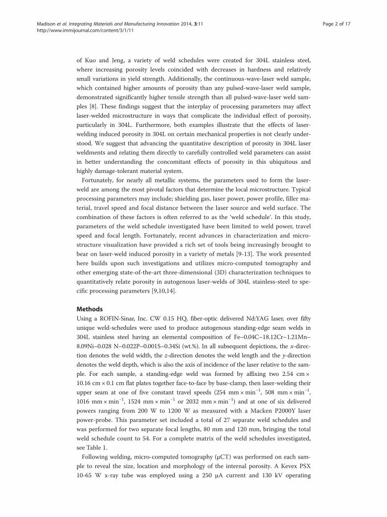
principal curvatures. This visualization technique is called the Interfacial Shape Distri-
bution (ISD) [20,22,23] and its descriptive legend is reproduced here for convenience,
Figure 3. For the purposes of this study, the “L” phase, as illustrated in the figure, corre-
sponds to the pores within welds (the figure was originally made for a solid–liquid sys-
tem). To interpret the ISD, it is useful to arrange the curvature pairings into four major
regions or categories. The uniqueness of these four categories is determined by the
combination of positive or negative signs of H and K. Patches in which both H and K
are positive correspond to Region 1, which are spherical or ellipsoidal with solid within.
Patches in which the H is positive and K is negative correspond to region 2. Region 3
consists of patches that have negative H and K values. Regions 2 and 3 contain saddle
shaped patches. Lastly, patches that have a negative H and positive K correspond to Re-
gion 4, which are spherical or ellipsoidal with the pore phase within. Based upon the
population of each principal curvature within one complete three-dimensional recon-
struction, which we will also refer to as a dataset, a probability can be assigned denot-
ing the likelihood of encountering a particular pairing of principal curvatures for a
given patch on the interface. It is important to note that the ISDs presented in this
study have not been normalized by any characteristic length-scale and therefore illus-
trate a combined effect of both shape and size. As a result, the color bar associated
with the ISDs presented later in the results section have units of μm2 so that the inte-
gration of the probability function over the entire ISD is equal to 1.
Figure 3 Interfacial Shape Distribution Legend indicating curvature types and their location withinthe ISD [20,22,23]. Reprinted from Acta Materialia, Vol. 54, issue 6, D. Kammer, P. Voorhees, “TheMorphological Evolution of Dendritic Microstructures During Coarsening”, pp. 1549–1558, (2006), withpermission from Elsevier.
Madison et al. Integrating Materials and Manufacturing Innovation 2014, 3:11 Page 6 of 17http://www.immijournal.com/content/3/1/11
Interfacial orientation
The interfacial normal n̂ð Þ associated with each interfacial patch of a dataset is used to
define a probability distribution for their orientation in three-dimensional space. The
method used to visualize this probability distribution is the Interfacial Normal Distribu-
tion or IND [23,24]. In this visualization technique, the two-dimensional projection of
a sphere with respect to a given axis displays the probability of occurrence of a given
normal orientation. In this study, all INDs are presented as projections along the posi-
tive z-axis, which is also the direction of travel for the work-piece beneath the welding
laser. Thus, the upper and lower hemispheres correspond to the direction toward and
away from the laser, respectively. The color values at each location in the IND indicate
the probability of encountering a particular normal based on the population of normals
within the dataset. The color bar associated with each IND presented later in the sec-
tion on results represents non-dimensional probability.
Spatial analysis
To better understand the spatial distribution of pore interfaces, we develop a method
to calculate interfacial-distance distributions (IDD) that provide the probability distri-
bution of the inter-pore distances, as measured between the pore surfaces nearest to
one another. In this paper, we refer to the IDD of the pores as “pore-interspacing distri-
bution” (PID). The method is based on the scheme for calculating the channel-size dis-
tributions of complex three-dimensional microstructures [26]. Further details regarding
this methodology will be available in a forthcoming publication. Briefly, to calculate the
interface-distance distribution, the image data of the 3D microstructure of the weld is
first converted to a signed distance function, the magnitude of which represents the
distance from the nearest pore-solid interface. The sign of the value indicates phase
within the dataset. In this study, points inside the pores are represented as positive

Madison et al. Integrating Materials and Manufacturing Innovation 2014, 3:11 Page 7 of 17http://www.immijournal.com/content/3/1/11
distances and points in the solid are represented as negative distances. Each isodistance
of a microstructure is an isosurface defined by thresholding the distance function asso-
ciated with the microstructure at a particular distance value. We refer to the regions
with distance function values greater than the threshold as “voids” to distinguish them
from the original pores as the sizes and topological characteristics of the voids differ
from those of the pores. (Note that the interface of the microstructure is described by
the isosurface with a threshold value of zero.) Topological changes in the isodistance
structure from one threshold to another denote the feature sizes of the structure. The
differences between isodistance structures resulting from thresholding in the positive
and negative directions are illustrated in the two-dimensional schematics of Figure 4,
where the value of the distance function is represented by grayscale and the isocontour
(analogous to isosurface in three dimensions) of each threshold value is marked by a
black line.
When the isodistance structures join together from thresholding with a negative
threshold value, a change in the number of voids arises. This occurs at a distance value
corresponding to half of the pore interspacing (the distance between interfaces at the
narrowest point). Since we are examining systems that contain a variety of spatial dis-
tributions of pores, PIDs are calculated by measuring the rate at which pores are join-
ing as a function of the distance threshold. Specifically, the PID is calculated by taking
the negative derivative (−1 times the derivative) of the number of voids as a function of
twice the distance threshold. Numerically, a central differencing method is used to cal-
culate the derivatives. Each point in the PID represents the probability of finding a pair
of pores with the pore interspacing at the corresponding distance threshold value.
(a) (b)
(d) (e) (f)
threshold distance = 0 threshold distance = 3 threshold distance = 5
15
10
5
0
threshold distance = 0 threshold distance = 2 threshold distance = 3
15
10
5
0
(c)
Figure 4 Two-dimensional schematic of the isodistance structures of two circular pores embeddedin a uniform matrix where grayscale represents the values of the distance function. The interfaces ofthe two pores are denoted by the black lines at a threshold value of zero, (a) and (d). Isocontour structures(isodistance structures in three dimensions) become smaller with increasingly positive threshold values (b)and eventually disappear when the threshold value exceeds the radius of the pore (c). Isocontour structuresbecome larger with increasingly negative threshold values (e) and eventually join together when themagnitude of the threshold value exceeds one half of the nearest distance between the two pores (f),causing a change in the number of voids.

Madison et al. Integrating Materials and Manufacturing Innovation 2014, 3:11 Page 8 of 17http://www.immijournal.com/content/3/1/11
Furthermore, a characteristic pore interspacing is calculated by taking the weighted
mean of the pore interspacing.
Similarly, when the isodistance structures are created for positive threshold values, a
change in the number of voids also arises when the threshold becomes larger than the
largest distance function value within a pore. The corresponding distance value is half
the smallest dimension (the radius for a sphere) of the pore. Once again, measuring the
rate at which pores disappear as a function of the distance threshold gives a pore-size
distribution. Lastly, the characteristic pore interspacing is scaled to yield solid linear
fraction (SLF):
SLF ¼ Rr þ R
ð3Þ
where R is one half of the characteristic pore interspacing and r is the characteristic
pore radius. The SLF provides a measure of local linear fraction of solid along the path
connecting the center of the particles and passing through the narrowest matrix region.
Unlike pore volume fraction, another commonly used measure of density, the SLF does
not depend on the volume used for the calculation. This is of particular note for each
weld schedule studied here, as laser weld porosity is generally a localized phenomena
often occurring at the centerline of the weld and not distributed homogeneously
throughout the weld. Furthermore, the SLF is useful as it yields a quantitative metric of
solid material between regions of densely populated pores relative to the size of pores
present. It is expected that this type of spacing sensitivity metric would have a strong
influence on the mechanical properties of the weld.
Results and discussionPopulation statistics
As mentioned previously, a variety of population metrics were extracted from each
weld schedule including but not limited to average and maximum pore volume, linear
frequency, and total number of pores observed per weld case. Average pore volume for
both focal lengths are shown in Figure 5 where each data series corresponds to a spe-
cific travel speed and data are presented as a function of delivered power. The trend is
consistent in that for a given travel speed, increases in welding power produce larger
pores. Slower travel speeds also generally produce larger pores with some exceptions to
this trend. Linear frequency was obtained by taking the total number of observed pores
for a given weld and dividing it by the weld length. Figure 6 illustrates a more complex
dependence of linear frequency on power and travel speed. With the exception of the
2032 mm×min−1 data series, an inflection point for the maximum frequency of pores
was observed across all series of travel speeds, indicating that fewer pores can be ob-
tained by increasing power delivered while maintaining the same travel speed. Further-
more, increases in travel speed shift the inflection point for diminishing pore presence
to higher powers. An inflection point may be observed for the 2032 mm ×min−1 travel
speed at higher powers as the data suggests an inflection point for this travel speed
may lie just beyond the bounds of this study. While the aforementioned trends are con-
sistent across both focal lenses, it is interesting to note that the 120 mm lens produces
higher average porosity volume (Figure 5) but generally lower frequencies (Figure 6) at
all parameter sets. In Table 1, maximum pore volume observed and total pore

Figure 5 Average pore volume as a function of weld power under (a) 80 mm focal lens and (b)120 mm focal lens showing an increase in pore volume with weld power and decreases intravel speed.
Madison et al. Integrating Materials and Manufacturing Innovation 2014, 3:11 Page 9 of 17http://www.immijournal.com/content/3/1/11
populations within each weld schedule are shown, with population counts denoted
within parentheses. No porosity was observed in any weld produced at 200 W nor at
higher travel speeds at 400 W under the 120 mm focal length.
Interfacial shape distributions
Interfacial shape distributions for porosity observed at 600 W across all five travel
speeds are shown for a focal length of 120 mm in Figure 7. All ISDs are plotted on a
uniform color scale in units of square microns to aid in comparison. In the discussion
in this section and those following, welds are grouped by travel speed into three cat-
egories: low (254 and 508 mm ×min−1), moderate (1016 mm ×min−1 only), and high
(1524 and 2032 mm ×min−1). At low travel speeds, the majority of interfacial patches
lie in Region 4 of the ISD, which largely corresponds to elliptical shapes with the edge
of the shape distributions reaching the κ1=κ2 line, which corresponds to completely
Figure 6 Pore frequency per unit length as a function of weld power under (a) 80 mm focal lensand (b) 120 mm focal lens.
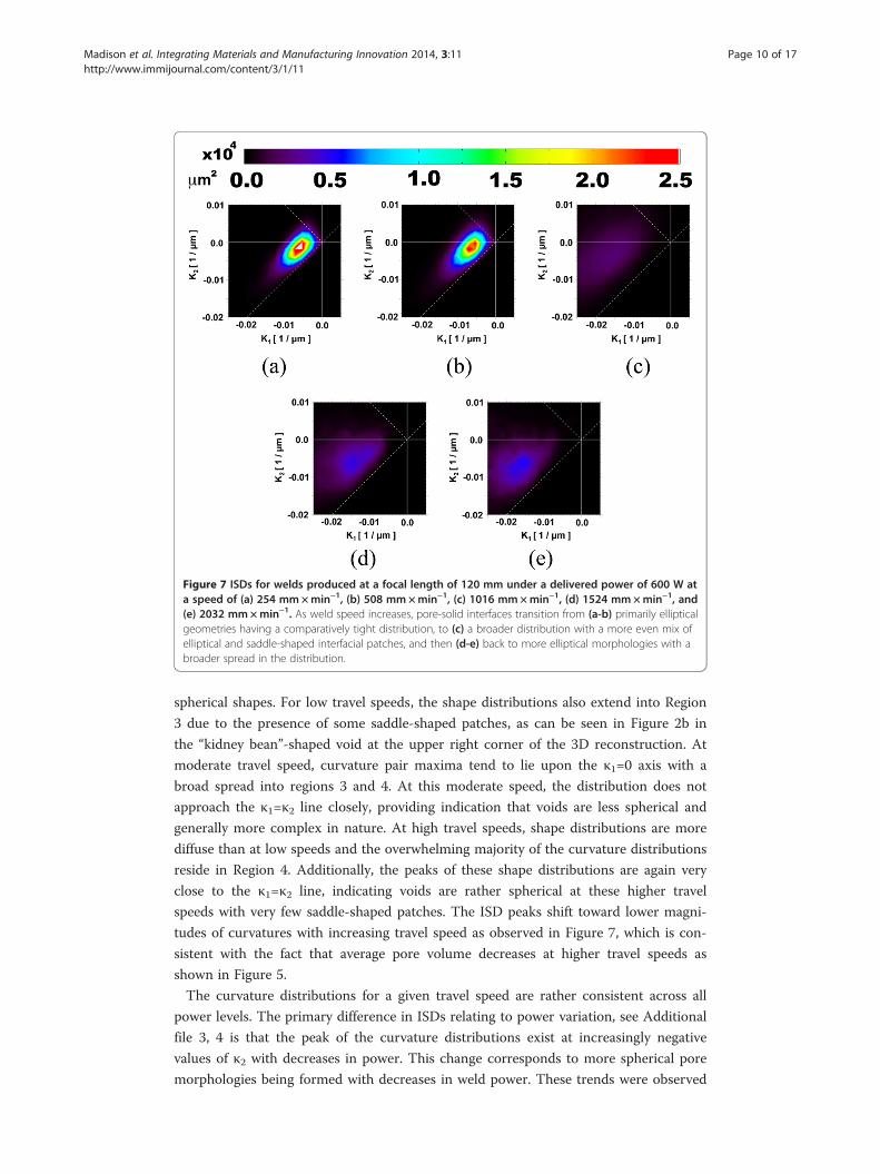
Figure 7 ISDs for welds produced at a focal length of 120 mm under a delivered power of 600 W ata speed of (a) 254 mm×min−1, (b) 508 mm×min−1, (c) 1016 mm×min−1, (d) 1524 mm×min−1, and(e) 2032 mm×min−1. As weld speed increases, pore-solid interfaces transition from (a-b) primarily ellipticalgeometries having a comparatively tight distribution, to (c) a broader distribution with a more even mix ofelliptical and saddle-shaped interfacial patches, and then (d-e) back to more elliptical morphologies with abroader spread in the distribution.
Madison et al. Integrating Materials and Manufacturing Innovation 2014, 3:11 Page 10 of 17http://www.immijournal.com/content/3/1/11
spherical shapes. For low travel speeds, the shape distributions also extend into Region
3 due to the presence of some saddle-shaped patches, as can be seen in Figure 2b in
the “kidney bean”-shaped void at the upper right corner of the 3D reconstruction. At
moderate travel speed, curvature pair maxima tend to lie upon the κ1=0 axis with a
broad spread into regions 3 and 4. At this moderate speed, the distribution does not
approach the κ1=κ2 line closely, providing indication that voids are less spherical and
generally more complex in nature. At high travel speeds, shape distributions are more
diffuse than at low speeds and the overwhelming majority of the curvature distributions
reside in Region 4. Additionally, the peaks of these shape distributions are again very
close to the κ1=κ2 line, indicating voids are rather spherical at these higher travel
speeds with very few saddle-shaped patches. The ISD peaks shift toward lower magni-
tudes of curvatures with increasing travel speed as observed in Figure 7, which is con-
sistent with the fact that average pore volume decreases at higher travel speeds as
shown in Figure 5.
The curvature distributions for a given travel speed are rather consistent across all
power levels. The primary difference in ISDs relating to power variation, see Additional
file 3, 4 is that the peak of the curvature distributions exist at increasingly negative
values of κ2 with decreases in power. This change corresponds to more spherical pore
morphologies being formed with decreases in weld power. These trends were observed
Madison et al. Integrating Materials and Manufacturing Innovation 2014, 3:11 Page 11 of 17http://www.immijournal.com/content/3/1/11
consistently across both focal length welds. A full set of calculated ISDs for all weld
cases in this study having more than twenty pores each are included in the Additional
file 3, 4 to this article.
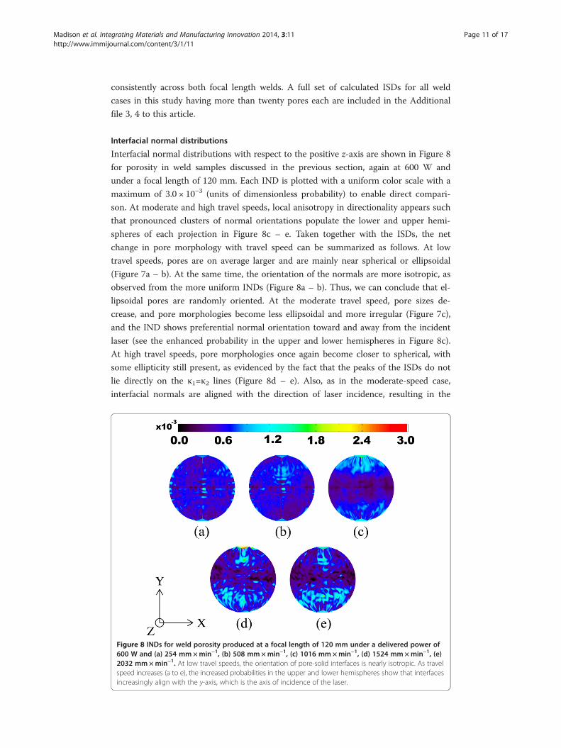
Interfacial normal distributions
Interfacial normal distributions with respect to the positive z-axis are shown in Figure 8
for porosity in weld samples discussed in the previous section, again at 600 W and
under a focal length of 120 mm. Each IND is plotted with a uniform color scale with a
maximum of 3.0 × 10⁻³ (units of dimensionless probability) to enable direct compari-
son. At moderate and high travel speeds, local anisotropy in directionality appears such
that pronounced clusters of normal orientations populate the lower and upper hemi-
spheres of each projection in Figure 8c – e. Taken together with the ISDs, the net
change in pore morphology with travel speed can be summarized as follows. At low
travel speeds, pores are on average larger and are mainly near spherical or ellipsoidal
(Figure 7a – b). At the same time, the orientation of the normals are more isotropic, as
observed from the more uniform INDs (Figure 8a – b). Thus, we can conclude that el-
lipsoidal pores are randomly oriented. At the moderate travel speed, pore sizes de-
crease, and pore morphologies become less ellipsoidal and more irregular (Figure 7c),
and the IND shows preferential normal orientation toward and away from the incident
laser (see the enhanced probability in the upper and lower hemispheres in Figure 8c).
At high travel speeds, pore morphologies once again become closer to spherical, with
some ellipticity still present, as evidenced by the fact that the peaks of the ISDs do not
lie directly on the κ1=κ2 lines (Figure 8d – e). Also, as in the moderate-speed case,
interfacial normals are aligned with the direction of laser incidence, resulting in the
Figure 8 INDs for weld porosity produced at a focal length of 120 mm under a delivered power of600 W and (a) 254 mm×min−1, (b) 508 mm×min−1, (c) 1016 mm×min−1, (d) 1524 mm×min−1, (e)2032 mm×min−1. At low travel speeds, the orientation of pore-solid interfaces is nearly isotropic. As travelspeed increases (a to e), the increased probabilities in the upper and lower hemispheres show that interfacesincreasingly align with the y-axis, which is the axis of incidence of the laser.

Madison et al. Integrating Materials and Manufacturing Innovation 2014, 3:11 Page 12 of 17http://www.immijournal.com/content/3/1/11
peaks of the INDs occurring in the upper and lower hemispheres at these high speeds.
The same trends were observed in the negative z-axis projections as well. Succinctly
stated, increasing weld speed results in decreased pore sizes and in interfacial normals
preferentially orienting in the direction of laser incidence (both toward and away from).
These trends in ISDs and INDs were observed across all powers and across both focal
lengths. For completeness, calculated INDs for all weld cases in this study are also in-
cluded in the Additional file 5, 6, 7 and 8 to more fully demonstrate the trend.
Pore interspacing
The pore-interspacing and pore-size distributions were calculated for a total of 18 weld
schedules to more closely examine the interspacing of pores in three dimensions as a
function of weld power and weld speed. These cases span both focal lenses and include
welds for which power was varied while travel speed was held constant at 1016 mm ×
min−1 and for which the travel speed was varied for a constant power of 600 W; see
Table 2. These selections traverse the central column and row of both sample matrices
where porosity was observed, shown in Table 1, encompassing median values for mm-
scale laser-welds. The probability distributions in Figures 9 and 10 were calculated as
described in the section on spatial analysis. To alleviate redundancy, PIDs for only the
120 mm focal length welds are plotted in Figure 9, as the trends illustrated here are
consistent for the 80 mm focal length results as well. In Figure 9, each data series rep-
resents a speed of 1016 mm ×min−1 under a different power. Overall, the pore-
interspacing probability distributions shift to higher values of distances as the weld
power increases. Stated simply, pores are spaced farther apart at higher power.
Pore interspacing was also calculated for various weld speeds, as shown in Figure 10.
Again, to reduce redundancy and to make the trend clear, only select results are shown
for welds made at multiple speeds in conjunction with the 120 mm focal length at
600 W. While the probability of finding pores at interspacing distances below 250 mi-
crons is relatively high across all cases, the distributions appear to be broader for low
and high travel speeds, with the high travel-speed case potentially exhibiting a bimodal
Table 2 Pore interspacing, radius and SLF as functions of weld power and speed
80 mm lens 120 mm lens
Weld power(W)
Pore interspacing(μm)
Pore radius(μm)
SLF Pore interspacing(μm)
Pore radius(μm)
SLF
400 300 (14.8) 51 (7.4) 0.75 (0.05) – – –
600 124 (9.1) 52 (4.6) 0.54 (0.05) 78 (9) 41 (4.5) 0.49 (0.07)
800 144 (9.2) 69 (4.6) 0.51 (0.04) 107 (9) 88 (4.5) 0.38 (0.04)
1000 170 (14.2) 82 (7.1) 0.51 (0.05) 110 (14.6) 104 (7.8) 0.35 (0.05)
1200 240 (15.5) 89 (7.8) 0.58 (0.05) 210 (20) 120 (10) 0.47 (0.05)
Weld speed(mm×min−1)
Pore interspacing(μm)
Pore radius(μm)
SLF Pore interspacing(μm)
Pore radius(μm)
SLF
252 270 (14.8) 108 (7.4) 0.55 (0.04) 340 (14.6) 129 (7.8) 0.57 (0.04)
510 170 (14.8) 142 (7.4) 0.37 (0.04) 160 (14.6) 124 (7.8) 0.40 (0.04)
1016 124 (9.1) 52 (4.5) 0.54 (0.05) 78 (9) 41 (4.5) 0.49 (0.07)
1524 110 (14.3) 63 (7.1) 0.47 (0.07) 230 (14.6) 51 (7.8) 0.70 (0.06)
2032 190 (14.3) 57 (7.1) 0.62 (0.06) 310 (14.6) 58 (7.8) 0.72 (0.05)
Variable weld powers shown are for a constant travel speed of 1016 mm ×min−1 and variable weld speeds shown are fora constant power of 600 W.

Figure 9 Pore-interspacing distributions with variation in power for 120 mm focal length weldseries. The probability distribution shifts to higher values of distances as weld power is increased.
Madison et al. Integrating Materials and Manufacturing Innovation 2014, 3:11 Page 13 of 17http://www.immijournal.com/content/3/1/11
distribution. However, the statistics are insufficient to conclusively determine whether a
bimodal distribution exists; further examination of larger weld samples or a larger
number of samples under the same processing parameters are required to do so.
The characteristic pore interspacing, characteristic pore radius, and SLF are listed in
Table 2 for all pore structures considered in Figures 9 and 10. To better illustrate the
variation with process parameters, calculated SLF are plotted as functions of delivered
power and weld speed across all process pairs examined in Figure 11. The method for
calculating pore interspacing and radius is accurate up to half a voxel [26]. Therefore,
the accuracy of each calculation is dependent on the resolution of the measurements;
the uncertainty is listed within parenthesis in Table 2 and shown by error bars in
Figure 11.
As described earlier, pore interspacing is a measure of the proximity of pores in the
weld structure, while the SLF measures the proximity of pores relative to the distance
between their centers and the characteristic pore size. For the samples where weld
power is varied, the smallest pore interspacing was found at 600 W for a speed of
Figure 10 A comparison of pore-interspacing distributions with varying weld speed for 120 mmfocal length at 600 W. At the high (2032 mm×min−1) and low (254 mm×min−1) speeds, several poresare found at large distances from one another, while at the medium (1016 mm×min−1), weld speed poresare clustered relatively closely.

Figure 11 SLF as a function of weld (a) power and (b) speed. With respect to variations in travel speed,minimum SLF was observed to occur at 510 mm×min−1. With respect to variations in power, SLF waslowest in the range of 800–1000 W, which is noteworthy as this range of powers coincides with theparameters that produce high pore frequencies per unit length across all weld schedules investigated(see Figure 6). The error bars show the calculation uncertainty presented in parenthesis in Table 2.
Madison et al. Integrating Materials and Manufacturing Innovation 2014, 3:11 Page 14 of 17http://www.immijournal.com/content/3/1/11
1016 mm×min−1 for both 80 and 120 mm lens welds (see Table 2), while the minimum
SLF occurs at weld powers of 800 – 1000 W for the same travel speed (Figure 11a). This
is consistent with the results of Figure 6, where the structure with the highest pore fre-
quency per unit length arises at a weld power of 800 W for the 1016 mm×min−1 speed
weld series. While these results are consistent, SLF provides a more insightful detail of the
pore structures present; for example, in the case of 800 W welds formed at 1016 mm×
min−1 with a 120 mm focus lens, the pore interfaces are separated by a distance that is
0.39 times the center-to-center distance between neighboring pores on average. Addition-
ally, it is valuable to point out that the SLF is in the range of 0.4 to 0.6 for welds with a
broad range of process parameters, which indicates that characteristic pore interspacing is
approximately the same as the characteristic pore diameter in these cases. This suggests that
for many weld cases, the characteristic pore interspacing can be approximated by the aver-
age pore diameter, which is generally easier to measure. However, high SLF values (> 0.6)
are observed at the lowest power and the highest speed, indicating that pores may be
spaced farther apart relative to their size at low delivered energy (Table 2 and Figure 11).
Pore size variability
The measures presented above are useful in quantifying the influence of specific weld
parameters on resultant pore microstructures. These measures revealed various degree
of variability within each weld. For example, ISDs are not sharply peaked, indicating
some pore surfaces have high curvatures while others have low curvatures. Here, we
examine the width of the distribution for pore sizes to better elucidate the variability in
this measure. To this end, the coefficient of variation (c.v.) associated with equivalent
pore radii is calculated. The coefficient of variation provides a quantitative measure of
the variability of any population by taking the ratio of the standard deviation (σ) to the
average (μ), Equation 4.
c:v: ¼ σ
μ¼
ffiffiffiffiffiffiffiffiffiffiffiffiffiffiffiffiffiffiffiffiffiffiffiffiffiffiffiffiffiffiffi1N
XN
i¼1xi−μð Þ2
q
μð4Þ
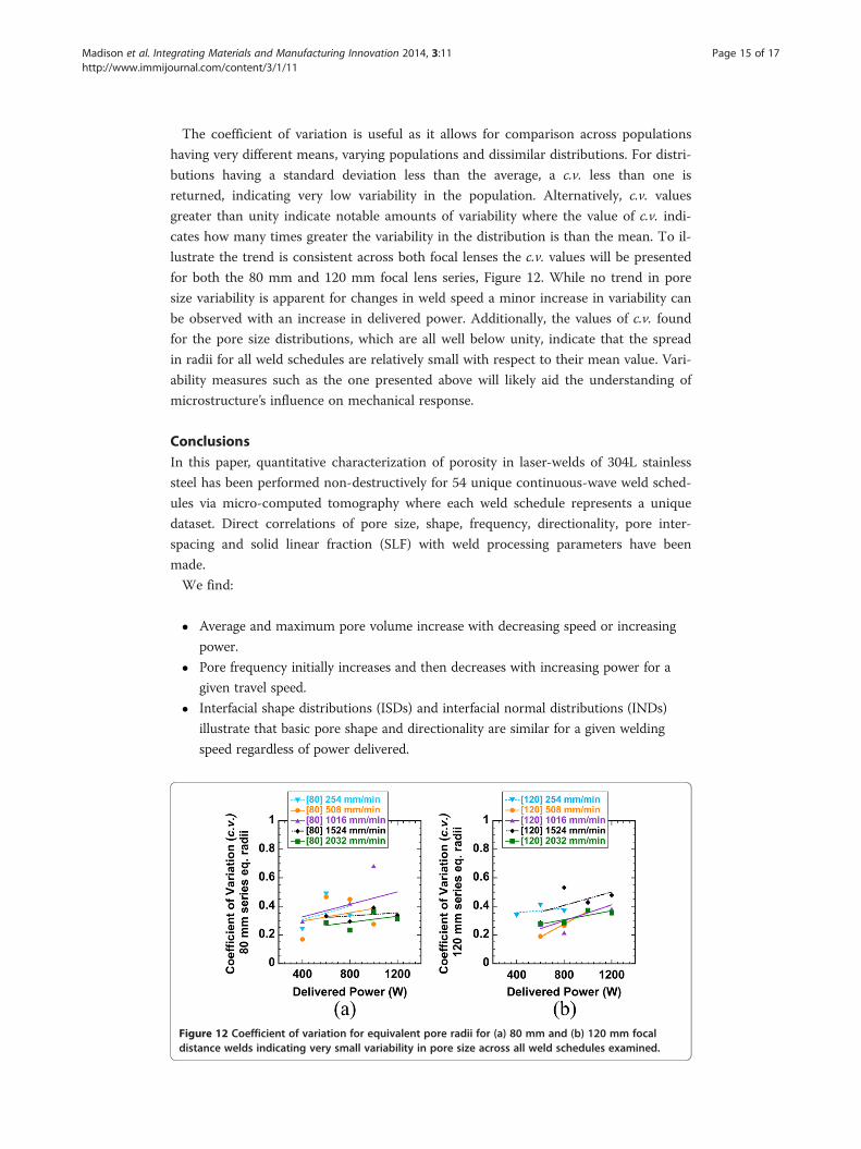
Madison et al. Integrating Materials and Manufacturing Innovation 2014, 3:11 Page 15 of 17http://www.immijournal.com/content/3/1/11
The coefficient of variation is useful as it allows for comparison across populations
having very different means, varying populations and dissimilar distributions. For distri-
butions having a standard deviation less than the average, a c.v. less than one is
returned, indicating very low variability in the population. Alternatively, c.v. values
greater than unity indicate notable amounts of variability where the value of c.v. indi-
cates how many times greater the variability in the distribution is than the mean. To il-
lustrate the trend is consistent across both focal lenses the c.v. values will be presented
for both the 80 mm and 120 mm focal lens series, Figure 12. While no trend in pore
size variability is apparent for changes in weld speed a minor increase in variability can
be observed with an increase in delivered power. Additionally, the values of c.v. found
for the pore size distributions, which are all well below unity, indicate that the spread
in radii for all weld schedules are relatively small with respect to their mean value. Vari-
ability measures such as the one presented above will likely aid the understanding of
microstructure’s influence on mechanical response.
ConclusionsIn this paper, quantitative characterization of porosity in laser-welds of 304L stainless
steel has been performed non-destructively for 54 unique continuous-wave weld sched-
ules via micro-computed tomography where each weld schedule represents a unique
dataset. Direct correlations of pore size, shape, frequency, directionality, pore inter-
spacing and solid linear fraction (SLF) with weld processing parameters have been
made.
We find:
� Average and maximum pore volume increase with decreasing speed or increasing
power.
� Pore frequency initially increases and then decreases with increasing power for a
given travel speed.
� Interfacial shape distributions (ISDs) and interfacial normal distributions (INDs)
illustrate that basic pore shape and directionality are similar for a given welding
speed regardless of power delivered.
Figure 12 Coefficient of variation for equivalent pore radii for (a) 80 mm and (b) 120 mm focaldistance welds indicating very small variability in pore size across all weld schedules examined.

Madison et al. Integrating Materials and Manufacturing Innovation 2014, 3:11 Page 16 of 17http://www.immijournal.com/content/3/1/11
� ISDs show that pore shapes are nearly spherical or ellipsoidal at low and high travel
speeds and are far more irregular, with a mix of ellipsoidal and saddle-shape geometries
at moderate travel speeds.
� INDs indicate that pore orientations become anisotropic at moderate to high travel
speeds with large concentrations of pore interfacial normals pointing toward and
away from the direction of laser incidence.
� Characteristic pore interspacing is nominally equivalent to characteristic pore
diameter for welds with a broad range of process parameters, as reflected in the
solid linear fraction (SLF) values.
� The values of c.v. indicate that the spread in pore radii is small with respect to their
mean value for all weld schedules.
� High travel speeds and low delivered power result in the lowest pore linear
frequency while increasing the amount of solid material between pores, which
would likely yield improved mechanical properties.
Availability of supporting dataAnimations of the five primary 3D reconstructions featured in this article for which
ISDs, INDs, pore interspacing and SLF were calculated and presented have been made
publicly available [27].
Additional files
Additional file 1: 3D Reconstructions of Porosity produced by laser-weld under a focal lens of 80 mm atvarious speeds and powers.
Additional file 2: 3D Reconstructions of Porosity produced by laser-weld under a focal lens of 120 mm atvarious speeds and powers.
Additional file 3: Interfacial Shape Distributions for Porosity produced by laser-weld under a focal lens of80 mm at various speeds and powers.
Additional file 4: Interfacial Shape Distributions for Porosity produced by laser-weld under a focal lens of120 mm at various speeds and powers.
Additional file 5: Equal Area Interfacial Normal Distributions with respect to the positive x axis for Porosityproduced by laser-weld under a focal lens of 80 mm.
Additional file 6: Equal Area Interfacial Normal Distributions with respect to the negative x axis for Porosityproduced by laser-weld under a focal lens of 80 mm.
Additional file 7: Equal Area Interfacial Normal Distributions with respect to the positive x axis forPorosity produced by laser-weld under a focal lens of 120 mm.
Additional file 8: Equal Area Interfacial Normal Distributions with respect to the negative x axis for Porosityproduced by laser-weld under a focal lens of 120 mm.
Competing interestsThe authors declare that they have no competing interests.
Authors’ contributionsJM coordinated data collection, performed image segmentation, created 3d reconstructions and made basiccharacterization measures for all datasets. ISD and IND calculations were performed by LA and JM. Pore Interspacingand SLF calculations were performed by VC and KT. All authors read and approved the final manuscript.
AcknowledgementsSandia National Laboratories is a multi-program laboratory managed and operated by Sandia Corporation, a whollyowned subsidiary of Lockheed Martin Corporation, for the US Department of Energy’s National Nuclear SecurityAdministration under contract DE-AC04-94AL85000. V.W.L. Chan and K. Thornton would like to acknowledge NSF DMRGrant # 0746424 “CAREER: Integrated Research and Education Program in Three-Dimensional Materials Science andVisualization.” The computational resources for calculations of pore interspacing and pore sizes were provided by theExtreme Science and Engineering Discovery Environment (XSEDE), which is supported by National Science Foundationgrant number OCI-1053575, under allocation No. TG-DMR110007.

Madison et al. Integrating Materials and Manufacturing Innovation 2014, 3:11 Page 17 of 17http://www.immijournal.com/content/3/1/11
Author details1Computational Materials & Data Science, Sandia National Laboratories, 87185 Albuquerque, NM, USA. 2MaterialsScience & Engineering, University of Michigan, 48109 Ann Arbor, MI, USA.
Received: 11 November 2013 Accepted: 21 March 2014Published: 29 April 2014
References
1. Mazumder J (1993) Laser-Beam Welding. In: ASM Handbook, Vol. 6. ASM International, Materials Park, OH,pp 262–2692. Webber T, Lieb T, Mazumder J (2011) Laser Beam Welding. In: ASM Handbook, Vol. 6A. ASM International,
Materials Park, OH, pp 556–5693. Boyce BL, Reu PL, Robino CV (2006) The constitutive behavior of laser welds in 304L stainless steel determined by
digital image correlation. Metall Mater Trans A 37A:2481–24924. Haboudou A, Peyre P, Vannes AB, Peix G (2003) Reduction of porosity content generated during Nd:YAG laser
welding of A356 and AA5083 aluminum alloys. Mater Sci Eng A A363:40–525. Feist WD, Tillack G-R (1997) Ultrasonic Inspection of Pores in Electron Beam Welds. In: European-American Workshop
Determination of Reliability and Validation Methods of NDE. BAM, Berlin, Germany. June 18–20 1997. vol 4. NDT.net6. Zhu X, Shyam A, Jones JW, Mayer H, Lasecki JV, Allison JE (2006) Effects of microstructure and temperature on
fatigue behavior of E319-T7 cast aluminum alloy in very long life cycles. Int J Fatigue 28:1566–15717. Shyam A, Picard YN, Jones JW, Allison JE, Yalisove SM (2004) Small fatigue crack propagation from micronotches
in the cast aluminum alloy W319. Scr Mater 50:1109–1114. doi:10.1016/j.scriptamat.2004.01.0318. Kuo TY, Jeng SL (2005) Porosity reduction in Nd-YAG laser welding of stainless steel and inconel alloy by using a
pulsed wave. J Phys D Appl Phys 38:722–728. doi:10.1088/0022-3727/38/5/0099. Madison J, Aagesen LK (2012) Porosity in Millimeter-Scale Welds of Stainless Steel: Three-Dimensional
Characterization. Sandia National Laboratories, Albuquerque, NM10. Madison J, Aagesen LK (2012) Quantitative characterization of porosity in laser welds of stainless steel. Scr Mater
67(9):783–786. doi:10.1016/j.scriptamat.2012.06.01511. Tucker JD, Nolan TK, Martin AJ, Young GA (2012) Effect of travel speed and beam focus on porosity in alloy 690
laser welds. JOM 64(12):1409–1417. doi:10.1007/s11837-012-0481-312. Norris JT, Perricone MJ, Roach RA, Faraone KM, Ellison CM (2007) Evaluation of Weld Porosity in Laser Beam Seam
Welds: Optimizing Continuous Wave and Square Wave Modulated Processes. Sandia National Laboratories,Albuquerque, NM
13. Norris JT, Robino CV, Hirschfeld DA, Perricone MJ (2011) Effects of laser parameters on porosity formation:investigating millimeter scale continuous wave Nd:YAG laser welds. Weld J 90:198–203
14. Madison JD, Aagesen LK, Battaile CC, Rodelas JM, Payton TKCS (2013) Coupling 3D quantitative interrogation ofweld microstructure with 3D models of mechanical response. Metallography, Microstructure and Analysis 2(6):359–363. doi:10.1007/s13632-013-0097-1
15. Matsunawa A, Kim J-D, Seto N, Mizutani M, Katayama S (1998) Dynamics of keyhole and molten pool in laserwelding. J Laser Apps 10(6):247–254. doi:10.2351/1.521858
16. Pang S, Chen L, Zhou J, Yin Y, Chen T (2011) A three-dimensional sharp interface model for self-consistent keyholeand weld pool dynamics in deep penetration laser welding. J Phys D 44:1–15. doi:10.1088/0022-3727/44/2/025301
17. Rai R, Elmer JW, Palmer TA, DebRoy T (2007) Heat transfer and fluid flow during keyhole mode laserwelding of tantalum, Ti-6Al-4 V, 304L stainless steel and vanadium. J Phys D Appl Phys 40:5753–5766.doi:10.1088/0022-3727/40/18/037
18. Zhou J, Tsai H-L (2007) Porosity formation and prevention in pulsed laser welding. Trans ASME 129:1014–1024.doi:10.1115/1.2724846
19. Alkemper J, Voorhees PW (2001) Three-dimensional characterization of dendritic microstructures. Acta Mater49:897–902
20. Mendoza R, Alkemper J, Voorhees PW (2003) The morphological evolution of dendritic microstructures duringcoarsening. Metall Mater Trans A 34A(3):481–489
21. Mendoza R, Savin I, Thornton K, Voorhees PW (2004) Topological complexity and the dynamics of coarsening. NatMater 3:385–388. doi:10.1038/nmat1138
22. Kammer D, Mendoza R, Voorhees PW (2006) Cylindrical domain formation in topologically complex structures. ScrMater 55(1):17–22. doi:10.1016/j.scriptamat.2006.02.027
23. Kammer D, Voorhees PW (2006) The morphological evolution of dendritic microstructures during coarsening. ActaMater 54(6):1549–1558. doi:10.1016/j.actamat.2005.11.031
24. Fife JL, Voorhees PW (2009) The morphological evolution of equiaxed dendritic microstructures duringcoarsening. Acta Mater 57:2418–2428. doi: 10.1016/j.actamat.2009.01.036
25. Meyer N, Desbrun M, Schroder P, Barr AH (2003) Discrete Differential-Geometry Operators for Triangulated2-Manifolds. In: Polthier K, Hege HC (ed) Visualization and Mathematics III. Springer, Berlin, Germany, pp 35–37
26. Chan VWL, Thornton K (2012) Channel size distribution of complex three-dimensional microstructures calculated fromthe topological characterization of isodistance structures. Acta Mater 60:2509–2517. doi:10.1016/j.actamat.2011.12.042
27. Madison JD, Aagesen LK, Chan VWL, Thornton K (2014) 3-Dimensional Reconstructions of Porosity from Laser-Welds of304L Stainless Steel at 600W and a Variety of Travel Speeds. http://hdl.handle.net/11115/243
doi:10.1186/2193-9772-3-11Cite this article as: Madison et al.: Advancing quantitative description of porosity in autogenous laser-welds of304L stainless steel. Integrating Materials and Manufacturing Innovation 2014 3:11.