Research Article Tracking- and Scintillation-Aware Channel

Research ArticleTracking- and Scintillation-Aware Channel Model forGEO Satellite to Land Mobile Terminals at Ku-Band

Ali M. Al-Saegh,1 A. Sali,1 J. S. Mandeep,2 and Alyani Ismail1

1Department of Computer and Communication Systems Engineering, Universiti Putra Malaysia (UPM),43400 Serdang, Selangor, Malaysia2Department of Electrical, Electronic and Systems Engineering, Universiti Kebangsaan Malaysia (UKM),43600 Bangi, Selangor, Malaysia

Correspondence should be addressed to Ali M. Al-Saegh; [email protected]

Received 28 March 2014; Accepted 9 July 2014

Academic Editor: Paschalis Sofotasios

Copyright © 2015 Ali M. Al-Saegh et al.This is an open access article distributed under theCreative CommonsAttribution License,which permits unrestricted use, distribution, and reproduction in any medium, provided the original work is properly cited.

Recent advances in satellite to land mobile terminal services and technologies, which utilize high frequencies with directionalantennas, have made the design of an appropriate model for land mobile satellite (LMS) channels a necessity. This paper presentsLMS channel model at Ku-band with features that enhance accuracy, comprehensiveness, and reliability. The effect of satellitetracking loss at different mobile terminal speeds is considered for directional mobile antenna systems, a reliable troposphericscintillation model for an LMS scenario at tropical and temperate regions is presented, and finally a new quality indicator modulefor different modulation and coding schemes is included. The proposed extended LMS channel (ELMSC)model is designed basedon actual experimental measurements and can be applied to narrow- and wide-band signals at different regions and at differentspeeds and multichannel states. The proposed model exhibits lower root mean square error (RMSE) and significant performanceobservation compared with the conventional model in terms of the signal fluctuations, fade depth, signal-to-noise ratio (SNR), andquality indicators accompanied for several transmission schemes.

1. Introduction

Therecent applications and services in the broadcasting satel-lite communication to land mobile terminal have increasedthe demand for higher data rate and thus higher transmissionfrequency. Therefore, land mobile satellite (LMS) channelestimation at high frequency has become a necessity todevelop efficient adaptive transmission models and tech-niques as solutions for channel impairments. Considerableinterest has been directed recently toward LMS commu-nication at Ku-band [1], which is the main concern ofthis study, owing to the high number of existing transpon-ders and the large amount of available bandwidth. Never-theless, Ku-band receivers require a high-gain directionalantenna [1]. A new generation of statistical LMS channelmodels capable of producing time series generative mod-els was initially introduced for lower frequencies, particu-larly for L and S bands. These models have replaced theones that solely provide cumulative distribution functions

(CDFs), which are insufficient for appropriate investigations[2].

The LMS channel condition at Ku-band depends onmobility impairments and tropospheric scintillation. Thelatter, which causes rapid fluctuations in satellite signallevel, occurs due to the irregularities in radio refractivityas the wave travels along different medium densities inthe troposphere [3, 4]. Several researchers [1, 2, 5–10] havecreated well-designed LMS channel models. The accuracyof the estimated models has increased notably over timethrough the addition of several features for approaching thereal-world environment along with recent LMS technologiesand services. This condition has motivated researchers, aswell as the authors of this paper, to design more reliable LMSchannel models.

However, existing channel models do not consider tropo-spheric scintillation under nonrainy conditions, which signif-icantly affect the signal performance at Ku-band, particularlyat high humidity regions, such as tropical areas [4].Moreover,

Hindawi Publishing CorporationInternational Journal of Antennas and PropagationVolume 2015, Article ID 392714, 15 pageshttp://dx.doi.org/10.1155/2015/392714

2 International Journal of Antennas and Propagation

these models do not consider the impairments caused bydifferent vehicle speeds at Ku-band for systems utilizingmobile directional antenna.Therefore, a comprehensive LMSchannel modeling that considers these significant impair-ments is needed to be designed with lower root mean squareerror (RMSE).

This paper presents a channel model for satellite toland mobile terminals based on actual measured channelconditions. The proposed model is referred to as extendedLMS channel (ELMSC) model. The term “extended” refersto four new features included in the model design. Firstly,the improvement is based on actual signal measurementsto enhance the accuracy and reliability of the previouslydeveloped multistate LMS model at Ku-band. Secondly, theimpairment attributed to the variable vehicular speeds ismodeled concerning the clear line-of-sight (LOS) and shad-owing scenarios. Thirdly, an LMS tropospheric scintillationmodel is developed. Lastly, a quality indicator module isdeveloped and added to the ELMSC model. The model con-siders tropospheric scintillation and vehicular environmentsas well as its application to narrow- and wide-band signalsworldwide because the LMS environment varies with respectto different regions in theworld, particularly in temperate andtropical regions.

The LMS channel characteristics and impairmentsregarding the mobility and tropospheric scintillationeffects are presented in the next section. The experimentalsetup is enlightened in Section 3 taking into account themobility impairments for different states accompanied withtropospheric scintillation. The proposed ELMSC model ispresented in Section 4. Section 5 provides a discussion ofthe results obtained from the measurements and proposedmodel, along with comparisons made concerning theexisting models. The conclusion is presented in Section 6.

2. LMS Channel Characterizationsand Impairments

Transmission parameters considerably affect the channelcharacteristics, the amount of signal attenuation, and thequality of service (QoS) of the LMS signal. In particular, thetransmitted frequency, bandwidth, and elevation angle exerteffects that should be identified by satellite system designersprior to the design process. The amount of signal attenuationis directly proportional to the carrier frequency and inverselyproportional to the elevation angle; thus, the signal qualityindication metrics, such as the signal-to-noise ratio (SNR)and energy of bit to noise ratio (𝐸𝑏/𝑁𝑜), are affected. Forsignal frequencies below 3GHz, ionospheric scintillation hasa paramount effect on signal performance. This effect beginsto disappear as the frequency increases above the said value[11]. The bandwidth effect will be explained in Section 2.1.The mobility impairments and channel states are presentedin Sections 2.2 and 2.3, respectively. The tropospheric scintil-lation effect is discussed in Section 2.4.

2.1. Bandwidth and Directional Antenna. The bandwidth ofthe signal is considered narrow-band when it is smaller than

the coherence bandwidth; otherwise, it is wide-band. Thecoherence bandwidth, which is inversely proportional to thedelay spread, is typically in the range of 7MHz to 11MHz at L-band and approximately 30MHz at EHF band [1, 12]. Underthe narrow-band condition, which is the most probablecondition in the LMS channel [13], the channel causes signalamplitude variations, whereas the time dispersion (timedelay of the received echoes) is insignificant. Under thewide-band condition, the channel not only causes variationsin signal amplitude but also experiences significant timedispersion in the received signal. This condition will causedistortion effects, such as frequency selectivity or intersymbolinterference; this distortion effect is attributed to the arrivalof the signal echoes at the receiver at different excess delayswith respect to the direct signal [2].

Practically, the radiation pattern of a directional antenna,which is commonly used in LMS scenarios at Ku-band, filtersout the echoes with significant delays; therefore, narrow-band models are typically employed for Ku-band signals fornarrow- and wide-band signals [1, 12, 14].

2.2. Mobility. Advanced technologies for satellite commu-nication services have resulted in a significant increase inmobile satellite terminals. This condition gave rise to thedemand for the estimation of the mobility effect on thesatellite link channel. Mobility impairments are typicallyproduced by the shadowing or blockage of signal energy,multipath, and antenna tracking error. Shadowing is usuallycaused by roadside trees, whereas blockage is normallycaused by surrounding tall buildings or bridges. The multi-path effect, which can be modeled by Rayleigh distribution[15], is primarily attributed to nearby buildings in urban areasor mountains.

These major factors affect the performance and qualityof the received signal and have motivated LMS systemdesigners to build well-formulated mobility channel modelsto predict the signal performance of mobile scenarios. Foraccurate modeling, the model design should be based onactual channel condition measurements. Thus, a number ofexperiments are conducted to compare the measured resultswith that of our estimatedmodel (discussed in Section 3).Thereceived signal strength in a tropical region is measured inconsideration of the scenarios of signal quality degradationusing a mobile receiver system mounted at the roof of a car.To the best of our knowledge, this is the first experimentconducted to determine the mobility effects on satellite linkchannel conditions in tropical regions.

2.3. Channel States and Conventional Model. According tothe type of impairments encountered during the movements,LMS channel models can be categorized into single-state andmultistate models [16, 17]. The single-state model describesthe signal level distribution of a specific propagation environ-ment over time, such as clear LOS, direct signal blockage, orshadowing states. Typically, in a single-state LMS channel, theunblocked LOS signal is modeled by Rice distribution. The

International Journal of Antennas and Propagation 3

Rice factor (𝐾) is defined as the ratio of carrier to multipathnormalized average power. Consider

𝐾 =𝑎2

2𝜎2, (1)

where 𝑎 is the amplitude of the direct signal and 𝜎 is thestandard deviation. If the signal is totally blocked, it is usuallyrepresented by Rayleigh distribution.

Meanwhile, several researchers have established single-state channel models that focus on the shadowing condition;they defined this state as a combination of two distributions.The most used models for the LMS scenario are Suzuki andLoo models, which have gained global attention [13]. Loomodel assumes that, in the case of shadowing, the Rician-distributed direct signal amplitude varies according to alog-normal distribution, and the received complex envelopeconsists of the sum of the two phasors. The model considersthe change in the phase caused by the Doppler effect, whichis practically detected by the omnidirectional antenna. Loomodel is applied to multistate LMS channel models at L andS bands [10, 16, 18]. Suzukimodel is a combination of Rayleighand log-normal distributions and is conventionally applied tothe modeling of multistate LMS channels at Ku-band usingdirectional antenna [1].

However, in a real-world environment, two or more LMSchannel states may occur during normal satellite terminalmovement.Therefore, the signal performance exhibits severalsignificant transformations in its characteristics over timeunlike the terrestrial scenario whose behavior is usuallydescribed by a single distribution [2]. In such case, multistatestatistical models should be used to design LMS channelmodels [2, 19].

Based on data obtained from measurement campaignsin Europe, Lutz et al. [8] designed a two-state model thatestimates the LMS signal performance under clear sky (Riciandistribution) and signal blockage (Rayleigh distribution)conditions. A high-state channel model is typically based onthe Markov chain approach [15, 19]. The Markov chain is astochastic model in which a system takes on discrete states.This approach is commonly used to model the variationsin signal performance attributed to shadowing or blockageeffects [10]. The correlation between rain impairment andmobility impairment at Ku-band is presented in [9]; theymodified the Rice factor to include the rainy sky scenario.

The first stochastic multistate model based on receivedsignal measurements at Ku-band was supported by the Euro-pean Space Agency (ESA) [1]. A three-state channel modelthat reflects the proper approach for the real-world environ-ment, including clear sky, shadowing, and blockage scenarioswith multipath effect, was employed. The model was builtbased on the measurement campaign in Germany with aconstant high speed of 120Km/h in a highway environmentand lower than 60Km/h in other environments. However, thereceiver antenna was mounted on a mechanically steerableplatform during measurements; this condition may causepointing misalignments and hence a high tracking accuracyerror.

The International Telecommunication Union (ITU) [20]recommended the use of a three-state model for statistical-approach LMS channel modeling. Moreover, [2] stated thatthe three-state model provides a tradeoff between complexityand accuracy. For the aforementioned reasons, a three-statechannel is utilized in the proposed model. Thus, the model iscompared with the conventional model [1] that also imple-mented the three-state scenarios at Ku-band, as explainedin the previous paragraph. Nevertheless, other states canbe added besides the aforementioned three states; however,this condition represents only special case modeling, such asthat presented in [10, 18], where a fourth state was added.The former described the fourth state as signal unavailabilityattributed to the failure of the satellite tracking process forvery low elevation angles (lower than 10∘), whereas the fourthstate of the latter represented multisatellite diversity (anglediversity).

2.4. Tropospheric Scintillation. Tropospheric scintillationoccurs inherently as the wave travels along different mediumdensities in the troposphere and causes rapid fluctuations insatellite signal level due to irregularities in radio refractivity[3, 21]. The standard deviation of fluctuations in tropicalregions differs from that in temperate regions owing totheir different related weather parameters, particularly thetemperature and humidity of the medium. Accordingly, thiscondition results in different satellite channel assessmentsand signal quality performance. However, tropical regionsare warmer and have higher relative humidity (𝐻𝑅) thantemperate regions for most time of the year [22]. ITU [23]claimed that the fade depth of tropospheric scintillation mayreach a few dBs based on its probability of exceedance time.

3. Experimental Setup

To achieve accurate channel estimation, the model designshould be based on the measured values of the LMS channelconditions. Several experiments were therefore conducted tomeasure the received signal level at the receiver (installedin a vehicle) at different mobility impairments. The impair-ments that occur typically in everyday life were consid-ered (Figure 1), namely, effects attributed to different vehiclespeeds (up to 150Km/h), shadowing by roadside trees, andblockage by crossroad bridges.

The experimental measurements obtained in the south-ernmost region of Kuala Lumpur in Malaysia are shown inFigure 2. The measurements are represented by the threestates listed in Table 1.

A mobile antenna system (upper right image of Figure 2)was used in the measurements setup mounted at the roof ofa car (upper left image of Figure 2). The system consists ofa 0.44m mobile autosteerable antenna pointed at MEASAT3/3A broadcasting satellite (91.5∘E) at 76.5∘ elevation angle. Ahigh tracking rate (75∘/sec) antenna was employed to reducethe tracking error as much as possible. The antenna systemalso includes a built-in motor and gyroscope to point to thesatellite automatically. The detection, filtering, and ampli-fication processes were performed by the antenna system


Table 1: Measurements scenarios.

State number Scenario Details

State 1 Clear sky/different speeds The vehicle moved at different speeds (from 0 km/h up to 150 km/h) during clearLOS. Measurements at zero speed (stationary) were obtained as well.

State 2 ShadowingThe vehicle moved at constant speed (40 km/h) under link shadowing by tall trees(approximately 12m tall and 7m away from the vehicle on the average) on theroadsides.

State 3 Blockage The vehicle moved at constant speed (40 km/h) under blockage by road bridges.

Scen

ario

1

Scenario 3

Scen

ario

2

Figure 1: LMS link scenarios.

Figure 2: Measurements campaign.

before the down conversion to L-band IF by a 9.75GHz localoscillator.

As the signals pass through the mobile antenna system,they are split into two directions as shown in Figure 3; the firstdirection is toward the decoder, and the second is toward thespectrum analyzer for data evaluation and analysis.

Meanwhile, the relative humidity was obtained on theday of the measurement campaign from theMalaysianMete-orological Department (MMD). The satellite and receiversystems parameters are listed in Table 2.

Typically, when the directional antenna is used, thereflections from buildings come from angles that are differentfrom those in the satellite direction. This condition causes

Table 2: LMS system parameters.

EIRP 57 dBWAntenna elevation angle 76.5∘

Polarization HorizontalAntenna local oscillator 9.75GHzRadio frequency (RF) 11.68GHzIntermediate frequency (IF) 1.93GHzAntenna diameter 0.44mAntenna tracking rate 75∘/s

Table 3: Channel states probabilities.

Probability Value

𝑃1

836

875= 0.955

𝑃221

875= 0.024

𝑃318

875= 0.021

the reflections from the buildings to be rarely measured[1]. The measurement campaign was conducted in highwayand suburban areas as shown in Figure 2. The areas containmany crossroad bridges, tunnels, and road toll counters(whose sheds cause signal blockages) as well as roadsidetrees that cause shadowing because of their dense leaves andbranches. During the continuous measurements, 837 datarecordings were obtained at a clear sky state at various vehiclespeeds, whereas 21 and 17 recordings were obtained duringsignal shadowing and blockage, respectively. The probabilityof accordance of each state is obtained depending on theaforementioned numbers of recordings and shown in Table 3.

The large number of measured samples is used in thecomparison with the measured data to improve the accuracyof the ELMSC model. However, the probability of each statecan be assumed in the design of the LMS channel modelaccording to the environment of the specified region ofinterest.

4. ELMSC Model

Fading channel model and characterization gain the outmostimportance for systems utilizing LMS link adaptive tech-niques and channel-aware modeling performance evaluationand assessment. The proposed model consists of severalsections as shown in Figure 4. These sections include the


Relative humidity

Mobile antenna system

SplitterSpectrum analyzer

Data storage

Decoder

Filter AmplifierDown

converterSteerable antenna

Local oscillator

Motor

Gyroscope

Figure 3: Measurement setup.

GN(0, 1)

GN(0, 1)

GN(0, 1)

GN(M, Σ)

HR

𝜎s

y(t)x(t)

×

×

×

×

×

+

+

+

j

a

P10

G𝑁/20

Ascint

𝜎BL

Filter

State series

Vehicle speed series

Rate conversion and interpolation

132

FSLQuality

indicator

AWGN

Total impairments

PSD estimator

Complementary blocks

Tropospheric scintillation

Multipath generator

IS

𝜎LOS

Mul

tista

te m

odel

Figure 4: Proposed ELMSC model.

multipath generation, the multistate model, the troposphericscintillation model, the complementary blocks, and the qual-ity indicator module. The model is designed based on theactual experimental measurements presented in Section 3.

In an actual LMS environment, channel output 𝑦(𝑡) canbe defined as

𝑦 (𝑡) = 𝑥 (𝑡) 𝑓 (𝑡) + 𝑛 (𝑡) , (2)

where 𝑥(𝑡) is the transmitted signal, 𝑓(𝑡) is the LMS channelfading, and 𝑛(𝑡) is the signal noise. The proposed ELMSCmodel imposes a comprehensive impairments estimation

effect which includes the impairments of mobility 𝑚(𝑡) andtropospheric scintillation 𝑠(𝑡). Consider

𝑓𝑚 (𝑡) = 𝑚 (𝑡) 𝑠 (𝑡) , (3)

where 𝑓𝑚(𝑡) is the total mobility impairments. The mobilityimpairments of the LMS channel include the attenuationattributed to the satellite terminal speed, shadowing orblockage attributed to physical obstacles in the link, and themultipath effect. In practice, both impairments are modeledseparately to produce the time series for correlated scintilla-tion and mobility impairments. Afterwards, their values arecorrelated according to the mobility state environment. The


details of the proposed model blocks are explained in thesubsequent subsections.

4.1. Multipath Generator. The diffused multipath fadingmodel can be characterized by Rayleigh distribution [15].Theenvelope is a result of the reflected signals from number ofpaths𝑁 as illustrated in (4). Consider

𝑟 (𝑡) =

𝑁

∑𝑖=1

𝐴 𝑖 (𝑡) exp [𝑗 Γ𝑖 (𝑡)] , (4)

where𝐴 𝑖(𝑡) is the reflected power of the 𝑖th signals and Γ𝑖(𝑡) isa coefficient that depends on angular Doppler frequency 𝜔𝐷as well as angle of arrival 𝛽 and phase 𝜙 as expressed in (5).Consider

Γ𝑖 (𝑡) = 𝜔𝐷 cos𝛽𝑖 (𝑡) + 𝜙 (𝑡) . (5)

Therefore, (4) can be rewritten as (6) or (7). Consider

𝑟 (𝑡) = 𝐴 (𝑡)

𝑁

∑𝑖

cos Γ𝑖 (𝑡) + 𝑗𝐴 (𝑡)𝑁

∑𝑖

sin Γ𝑖 (𝑡) , (6)

𝑟 (𝑡) = 𝑟𝐼 (𝑡) + 𝑗𝑟𝑄 (𝑡) , (7)

where 𝑟𝐼(𝑡) and 𝑟𝑄(𝑡) represent the inphase and quadraturecomponents of the Rayleigh distribution, respectively. Thesetwo components, as predicted by the central limit theorem,can be produced by first generating two, zero-mean whiteGaussian distributions [13, 24] as shown in Figure 4. Thestandard deviation 𝜎 varies with respect to the clear sky,shadowing, and blockage states because the fluctuation levelattributed to the multipath effect differs with respect to eachstate [13]. 𝜎 reaches the maximum in the blockage state andminimum in the state of clear LOS. Therefore, 𝜎 is includedin the multistate model (explained in Section 4.2).

Power spectral shaping is achieved by coloring “filtering”the resultant complex signal. The inphase and quadraturetrails are filtered with a Doppler filter to shape “reproduce”the Doppler effects for the fading channel attributed to themotion of the terminal. The filtering process is necessary insimulating the channel. Without this process, the resultantsignal variations would be unnaturally fast for a given satelliteterminal speed and would thus produce error bursts and dis-tribution of outage durations [25]. Therefore, a Butterworthfilter is used in the proposed model; this filter is commonlyused in LMS channel modeling because it provides a morerealistic approach [13, 24, 26, 27]. The filtering process isdesigned based on [13, 27].

4.2. Multistate Model. Three states, namely, clear LOS, shad-owing, and blockage states, were implemented in the ELMSCmodel. The model introduces one of the extensions of theELMSC model that represents the losses of satellite terminalattributed to movements at different speeds (𝐼𝑆); the newextension is applied to the clear LOS and shadowing states.

The cumulative distribution of the resultant signal shouldbe the weighted combination of the three states [10, 23].

Therefore, the probability behavior for the three states isexpressed in (8). Consider

𝑃 (𝑛 ≤ 𝑁) = 𝑃1𝑚1 + 𝑃2𝑚2 + 𝑃3𝑚, (8)

where 𝑛 is the sample number from the total number ofsamples𝑁. 𝑃𝑖 is the probability of occurrence of the 𝑖th state(𝑃1 + 𝑃2 + 𝑃3 = 1). The probabilities were obtained from theexperimental measurements as mentioned in Section 3 andwere used to generate random state series. The total time (ornumber of samples) of being in a specific state depends onthe probability of occurrence. The output discrete signal is aresult of switching between the generated signal samples ofthe aforementioned states according to the state series.

4.2.1. Clear LOS Signal Model. The signal received by themobile satellite terminal moving at different speeds in aclear (unblocked) channel environment is usually modeledwith Rician distribution as discussed in Section 2.3. Themodel includes the constant direct signal with multipathfluctuations. The latter, Rician multipath, is designed by firstmultiplying the resultant signal from the multipath modeldiscussed in Section 4.1 with its specific standard deviation(𝜎LOS). The direct signal component (𝑎) is then added to theRician multipath signal. 𝑎 is extracted using (1), where 𝐾represents the ratio between the direct signal level and thenoise floor level.Therefore, our assumption on the Rice factoris based on the actual measurements of the signal. Typically,the noise floor level is assumed based on the measurementsetup [1, 2].

Moreover, to estimate the signal losses that may occurbecause of the antenna tracking error attributed to terminalmovements, a new formula is proposed (see (9)) to estimatethe signal losses for satellite terminal movements at differentspeeds in dB based on the actual measurement explained inSection 3. Consider

𝐼𝑆 = 𝑘𝑎𝑠2+ 𝑘𝑏𝑠 + 𝑘𝑐, (9)

where 𝑠 is the satellite terminal speed in km/h and the con-stant values 𝑘𝑎, 𝑘𝑏, and 𝑘𝑐 are −4.667×10

−5, 1.468×10−2, and−1.364 × 10−3, respectively. These values were obtained withnonlinear curve-fitting optimization technique; the proposedformula provides accurate mobility impairment estimationwith a RMSE of 0.02407. Terminal speed is used as an inputto the module. This input series can be generated usingsinusoidal distribution random numbers with a minimumvalue of 0. The maximum value can be assumed based on thenature of the road of interest and its highest permitted speed.Moreover, the probability of speed values can be obtainedthrough statistical observations.

4.2.2. Shadowed Signal Model. The shadowing (state 2)attributed to roadside trees causes additional attenuation tothe received signal and thus results in a slow variation inthe direct signal simultaneous with the diffuse multipathcomponents. Typically, the shadowed signal at Ku-band ismodeled with the Suzuki model [1]. This model involves thecombination of log-normal and Rayleigh distributions.


Normal distribution signal 𝐺𝑁 is generated with itsspecific mean𝑀 and standard deviation Σ obtained from [1]in dB before being converted to a log-normal distributionusing the relation 10𝐺𝑁/20.The resultant signal passes throughtwo stages: rate conversation (to identify the slope of theenvelop and number of the added samples based on 𝑓𝑆 ofthe fast multipath fluctuations) and interpolation (addingsamples between two different leveled samples correspondingto the rate conversation and then convolution for envelopeshaping of the interpolated samples). In summary, these stepswere implemented to add an interpolated sloped envelopsample to approach the number of multipath samples and toavoid sharp multipath fluctuations. For periods with no statetransitions, this rate is utilized to generate rapid variationswith a low sampling period to account for the Doppler spreadbandwidth [13].

The multipath fluctuations of this state were generated asdiscussed in Section 4.1.The resultant combination of the twodistributions is then obtained to reflect the performance ofthe signal in the shadowing environment. The impairmentsthat occur primarily because of the antenna tracking errordue to the terminal movements, expressed in (9), affect theshadowed signal as well because the direct signal componentstill exists despite being shadowed. Therefore, in the case ofa partially shadowed environment (state 2), the 𝐼𝑆 module isalso involved in the simulated shadowed signal.

4.2.3. Blocked Signal Model. LMS signal blockage (state 3) istypically caused by bridges across the highway, sheds of theroad tolls counters, tunnels, or tall buildings in urban areas.The received signal power vanishes, and the fade depth canbe expressed by the noise floor level below the LOS.The LMSsignal blockage model is typically designed with Rayleighdistribution with specific standard deviation 𝜎BL as discussedearlier. Therefore, 𝜎BL is applied to the resultant fluctuatedsignal from the multipath model discussed in Section 4.1.Considering that the direct signal is totally blocked in thisstate, the signal would be unaffected by the 𝐼𝑆 module. Thestatus of the current state is obtained from state series blockas shown in Figure 4 to switch the 𝐼𝑆 module on during theclear LOS and shadowing states and off during the blockagestate.

4.3. Tropospheric Scintillation Model. Tropospheric scintil-lation depends on its standard deviation (𝜎𝑆) [21, 23]. Themodeling of tropospheric scintillation effect begins with thegeneration of a zero-mean white Gaussian distribution andwith standard deviation conventionally set to 1 [23, 28].However, 𝜎𝑆 depends mainly on the relative humidity andthe temperature [23], which is different in tropical regionscompared with temperate regions according to their weatherparameters. For temperate regions, Cioni et al. [28] assumedthat the value of 𝜎𝑆 is 0.066. However, it is declared by[22] that the standard deviation of scintillation in tropicalregions is larger than that in temperate regions. Therefore, 𝜎𝑆is adjusted to 0.117 to increase the accuracy of the estimatedscintillation standard deviation. The value of 𝜎𝑆 is estimatedbased on two steps. First, the𝐻𝑅 value was obtained from the

MMD as discussed in Section 3. Second, the mean value isused to estimate 𝜎𝑆 according to (10) [23]. Consider

𝜎𝑆 = 𝜎0 𝑓0.583 𝑔

(sin 𝜃)1.2, (10)

where 𝑓 is the frequency in GHz, 𝜃 is the angle of elevation,and 𝑔 is the antenna averaging factor that depends mainly onthe frequency and antenna parameters. 𝜎0 can be obtained indB from thewet term of radio refractivity𝑁wet which, in turn,depends on the value of temperature𝑇 and𝐻𝑅 [29]. Consider

𝜎0 = 0.0036 + 𝑁wet × 10−4,

𝑁wet = 3732 ×𝐻𝑅𝑒𝑆

𝑇2,

(11)

where 𝑒𝑆 is the temperature-dependent saturation vaporpressure that can be calculated from [29]. The mean value of𝐻𝑅measured byMMD is 82.375%.With 𝜎𝑆, the troposphericscintillation fade depth 𝐴 scint is estimated using the ITUmodel [23] for different probabilities of occurrence (𝑃).

The power spectral density (PSD) of the fading is timevariant and can be approximated by low-pass filter (LPF)[28]. The LPF in [28] is used, and the resultant signal is thenuniformly distributed and combined with𝐴 scint to obtain theestimated signal series of tropospheric scintillation.

4.4. Complementary Blocks and Quality Indicator. The totalperformance of the correlated impairments is a combinationof the LMSmultistate mobility and tropospheric scintillationmodels as declared in (2). However, as the signal passesthrough the channel, several other constraints cause addi-tional losses, such as system loss and free space loss (FSL).Thelatter depends on the transmitted frequency and the distancedifference between the satellite and the mobile terminal asrevealed in (12). Consider

FSL = 20 log(4𝜋𝑑𝜆

) . (12)

Consequently, the estimation of the received SNR, which isthe received signal power 𝑃𝑟 to noise [𝑃𝑛 = 10 log(𝑘𝐵TBW)]

ratio is included in the design. Equation (13) [30, 31] is utilizedto estimate the received power 𝑃𝑟 in dBW. Consider

𝑃𝑟 = EIRP + 𝐺𝑟 − FSL − 𝐿𝑆 − 𝐿LMS, (13)

where EIRP is the effective isotropic radiated power in dBWthat depends on the transmitted power and the transmitterantenna gain; 𝐺𝑟 is the receiver gain; 𝐿𝑆 is the total systemloss; and 𝐿LMS is the total LMS channel loss that has notbeen considered in previous studies, which represents thetotal fading losses that can be obtained from the ELMSCmodel. After the insertion of the channel fading effect to thetransmitted signal, additive white Gaussian noise (AWGN) isadded.

The atmospheric impairments have a negative effect onthe data after being demodulated in the receiver. The effectappears, for example, as a decrease in 𝐸𝑏/𝑁𝑜 or packet error


rate. These ratios can be utilized to generate the proposedindexing for optimal physical or link layer adaptations forthe current instantaneous transmission time interval (TTI).Equation (14) is used to obtain 𝐸𝑏/𝑁𝑜 (in dB) for widely usedmodulation schemes and code rates (MODCOD) in satellitecommunications. Consider

𝐸𝑏

𝑁𝑜=𝐸𝑆

𝑁𝑜− 10 log (𝐾) , (14)

𝐸𝑆

𝑁𝑜= SNR + 10 log(BW

𝑅) , (15)

where 𝐾 = log2(𝑀) × 𝑅𝐶, 𝑀 is the modulation order, 𝑅𝐶

is the code rate, 𝐸𝑠/𝑁𝑜 is the symbol energy to noise ratio,BW is the bandwidth, and 𝑅 is the symbol rate. For fixed 𝑅and BW, 𝐸𝑏/𝑁𝑜 is directly proportional to SNR and inverselyproportional to𝑀 and𝑅𝐶.Therefore, after substituting ((12)–(14)) to (15), the estimated𝐸𝑏/𝑁𝑜 is obtained as shown in (16).Consider

𝐸𝑏

𝑁𝑜= EIRP + 𝐺

𝑇− 20 log(4𝜋𝑑

𝜆) − 𝐿LMS

− 𝐿𝑆 − 𝑘𝐵 + 10 log(𝐾

𝑅) ,

(16)

where 𝐺/𝑇 is the figure of merit of the receiver antenna and𝑘𝐵 is the Boltzmann constant. 𝐸𝑏/𝑁𝑜 is used as a qualityindicator for the ELMSC model.

5. Results and Discussion

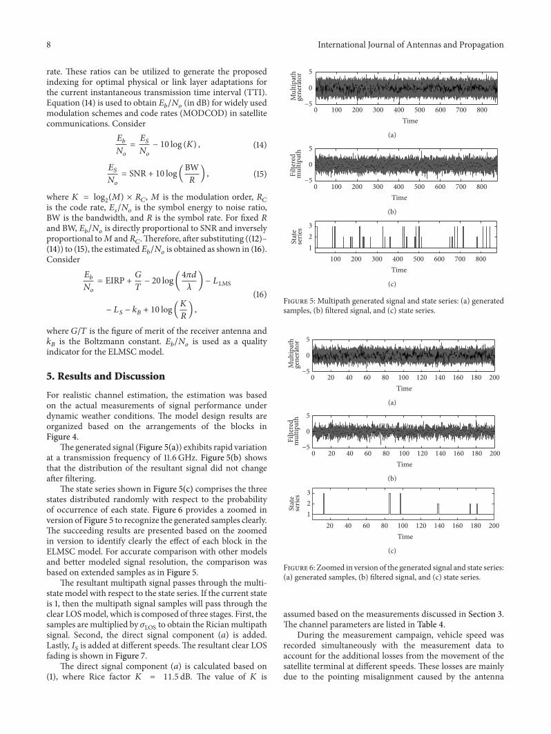
For realistic channel estimation, the estimation was basedon the actual measurements of signal performance underdynamic weather conditions. The model design results areorganized based on the arrangements of the blocks inFigure 4.

The generated signal (Figure 5(a)) exhibits rapid variationat a transmission frequency of 11.6 GHz. Figure 5(b) showsthat the distribution of the resultant signal did not changeafter filtering.

The state series shown in Figure 5(c) comprises the threestates distributed randomly with respect to the probabilityof occurrence of each state. Figure 6 provides a zoomed inversion of Figure 5 to recognize the generated samples clearly.The succeeding results are presented based on the zoomedin version to identify clearly the effect of each block in theELMSC model. For accurate comparison with other modelsand better modeled signal resolution, the comparison wasbased on extended samples as in Figure 5.

The resultant multipath signal passes through the multi-state model with respect to the state series. If the current stateis 1, then the multipath signal samples will pass through theclear LOSmodel, which is composed of three stages. First, thesamples are multiplied by 𝜎LOS to obtain the Ricianmultipathsignal. Second, the direct signal component (𝑎) is added.Lastly, 𝐼𝑆 is added at different speeds. The resultant clear LOSfading is shown in Figure 7.

The direct signal component (𝑎) is calculated based on(1), where Rice factor 𝐾 = 11.5 dB. The value of 𝐾 is

0 100 200 300 400 500 600 700 800−5

0

5

Mul

tipat

hge

nera

tor

Time

(a)

0 100 200 300 400 500 600 700 800−5

0

5

Filte

red

mul

tipat

h

Time

(b)

100 200 300 400 500 600 700 800 1 2 3

Time

Stat

ese

ries

(c)

Figure 5: Multipath generated signal and state series: (a) generatedsamples, (b) filtered signal, and (c) state series.

0 20 40 60 80 100 120 140 160 180 200−5

0

5

Mul

tipat

hge

nera

tor

Time

(a)

0 20 40 60 80 100 120 140 160 180 200−5

0

5

Filte

red

mul

tipat

h

Time

(b)

20 40 60 80 100 120 140 160 180 200 1 2 3

Time

Stat

ese

ries

(c)

Figure 6: Zoomed in version of the generated signal and state series:(a) generated samples, (b) filtered signal, and (c) state series.

assumed based on the measurements discussed in Section 3.The channel parameters are listed in Table 4.

During the measurement campaign, vehicle speed wasrecorded simultaneously with the measurement data toaccount for the additional losses from the movement of thesatellite terminal at different speeds. These losses are mainlydue to the pointing misalignment caused by the antenna


Table 4: Models’ parameters.

Parameter ELMSC Conventional [1]Satellite orbit GEO GEOFrequency band Ku KuRice 𝐾 factor 11.5 dB 17 dBClimatic area Temperate-tropical TemperateAntenna type Directional antenna Directional antenna

0 20 40 60 80 100 120 140 160 180 200Time

Fadi

ng (d

B)

0

−8

−6

−4

−2

2

4

6

8

10

−10

Figure 7: Fading in the clear LOS state.

tracking error. The resultant average measurement data ofsignal attenuation with respect to satellite terminal speed isshown in Figure 8.

With respect to terminal speed, the average values ofseveral measured signal samples have been obtained. Thespeed of approximately 40, 80, 100, 120, 140, and 150 km/hhas been considered in the measurement campaign as well asthe stationary (zero speed) case.Themeasurements show thatthe signal is further attenuated by 0.6 dB when the terminalmoves at 60 km/h. The attenuation slope changes when thespeed reaches 80 km/h. The attenuation level increases moreslightly than when speed is below 80 km/h. The losses reachapproximately 1 dB at 100Km/h, 1.15 dB at 140Km/h, and1.18 dB at 150Km/h. However, as discussed in Section 4.2 andexpressed in Figure 8, the proposed equation (9) providesan accurate estimation of signal performance at differentterminal speeds with RMSE equal to 0.02407. To the best ofour knowledge, this model is the first to be designed for theestimation of LMS channel impairments at different terminalspeeds based on measurement data at the Ku-band.

Based on the experimental measurements in the clearLOS scenario, the signal model at state 1 provides less RMSEestimation than the conventional model proposed earlier.This finding can be clearly proven by comparing the CDFand PDF of the measured SNR and the conventional modelwith the proposed model. After adding the effect of FSL from(12) to obtain the channel fade and AWGN to the transmittedsignal carrier, the CDF and PDF of the estimated receivedpower were obtained as shown in Figure 9.

To identify the effect of the proposed multistate part ofthe ELMSC model with respect to the clear LOS measuredsignal and conventional model, Figure 9 shows the CDF and

20 40 60 80 100 120 1400Speed (km/h)

Atte

nuat

ion

(dB)

Average measuredEstimated

1.2

1

0.8

0.6

0.4

0.2

0

Figure 8: Signal losses with respect to satellite terminal speed.

PDF of the received SNRprior to the addition of the proposedtropospheric scintillation model. The effect of the proposed𝐼𝑆 module appeared as a change in the slope difference ofCDF as shown in Figure 9(a). This leads to a decrease in theRMSE of the proposed model, whereas the change in the 𝐾factor shifted the CDF for few dBs towards the measuredvalue, which approaches the CDF slope of the measuredSNR comparedwith the conventionalmodel. Until this point,the PDF performance of the proposed model exhibits asignificant enhancement compared with the conventionalmodel such that it approaches the PDF of the measured SNRand will be further enhanced if tropospheric scintillation isincluded.

In the case of state 2, the shadowing model is appliedto the generated multipath signal in Figure 5(b). The modelis a combination of two distributions. The slow variationtrail is composed of three stages before the addition of rapidvariation. Finally, the signal passes through the proposed 𝐼𝑆block as discussed in Section 4.2. The effect of these steps isshown in Figure 10.

The slow variation trail begins with the generation ofrandom normal distribution samples. One of the objectivesof the experimental measurements is to measure the averagepower absorption for each scenario. 13 dB mean value is usedas proposed in [32].

The distribution is then converted to a log-normal distri-bution before rate conversion and interpolation as discussedin Section 4.2 and shown in Figure 10(a). Figure 10(b) showsthat the signal variation performance does not change afterthis step, except for the higher number of samples thataccounts for the generated rapid variations. Figure 10(c)shows the simulated shadowing fade.

The signal level in a full blocking environment (state3) usually reaches the noise floor level, as discussed inSection 4.2, with multipath fluctuations of specific standarddeviation 𝜎BL that is typically greater than 𝜎LOS [13]. There-fore, the resultant signal from the multipath generator ismultiplied by the value of 𝜎BL, which is assumed according to


9 10 11 12 13 14 15 16 17 180

0.10.20.30.40.50.60.70.80.9

1

SNR (dB)

CDF

Measured

ConventionalWith proposed IS

(a)

9 10 11 12 13 14 15 16 17 180

0.1

0.2

0.3

0.4

0.5

0.6

SNR (dB)

PDF

Measured

ConventionalWith proposed IS

(b)

Figure 9: Received SNR in clear LOS state: (a) CDF and (b) PDF.

05

1015

20 40 60 80 100 120 140 180160 200Time

Slow

var

iatio

nlo

g-no

rmal

(a)

05

1015

Afte

r rat

e con

vers

ion

and

inte

rpol

atio

n

20 40 60 80 100 120 140 180160 200Time

(b)

20 40 60 80 100 120 140 180160 200−50−40−30−20−10

010

Time

Shad

owin

gfa

de (d

B)

(c)

Figure 10: Simulated fade attributed to shadowing: (a) the generated slow variation lognormal distribution, (b) signal after rate conversionand interpolation, and (c) the aggregated fade.

[1]. However, the simulated signal of the multistate model isa result of the switching process of the three aforementionedstates. Switching control is based on the state series generated(shown in Figure 5(c)).

Another remarkable impairment to the LMS channel istropospheric scintillation which gives rise to signal turbu-lence because of the rapid change in the refractive index of themedium.The change in the refractive index of the medium isbecause of the water particles in the troposphere. Therefore,

the 𝐻𝑅 percentage has a vital role in the signal performanceand standard deviation of fluctuations.

𝐻𝑅 is varied from one region to another according totheir different weather parameters. Therefore, two differentsignals were modeled each with its specific region, one withlower standard deviation of fluctuation as proposed by [28]represents a temperate region and the other proposed in thisstudy for higher humidity regions as in tropics based on themeasured 𝐻𝑅 discussed in Section 4.3. Figure 11 shows the


−2

−1

0

1

2Tr

opos

pher

ic sc

intil

latio

nin

tem

pera

te re

gion

(dB)

0 20 40 60 80 100 120 140 160 180 200Time

(a)

0 20 40 60 80 100 120 140 160 180 200−2−1

012

Time

Trop

osph

eric

scin

tillat

ion

in tr

opic

al re

gion

(dB)

(b)

Figure 11: Modeled fluctuations caused by tropospheric scintillation: (a) temperate region and (b) tropical region LMS link scenarios.

9 10 11 12 13 14 15 16 17 180

0.10.20.30.40.50.60.70.80.9

1

SNR (dB)

CDF

ELMSC in temperate regionELMSC in tropical regionConventional

With proposed IS

(a)

9 10 11 12 13 14 15 16 17 180

0.1

0.2

0.3

0.4

0.5

0.6

SNR (dB)

PDF

ELMSC in temperate regionELMSC in tropical regionConventional

With proposed IS

(b)

Figure 12: Tropospheric scintillation effect: (a) CDF and (b) PDF.

estimated tropospheric scintillation performance accordingto the proposed model.

Figure 11 shows the difference in the estimated signalsamples between temperate and tropical regions. To identifythe effect of tropospheric scintillation clearly in both regions,Figure 12 shows the CDF and PDF of the received SNR intemperate and tropical regions for clear LOS state after addingthe tropospheric scintillation effect.

It is shown in Figure 12 that the distribution of thesamples in tropical regions is different from the temperateregions according to its weather parameters especially thehigher relative humidity and hence higher water particleswhich cause extra fluctuations compared with the temperateregions. Therefore, the fluctuation performance reflects achange in CDF and PDF with respect to the original distri-bution functions when tropospheric scintillation is excluded.It can be noticed that the peak value of the PDF of theestimated SNR in tropical region is moved to lower SNRbecause of the different weather parameters and approachesthe peak value of the measured SNR (as seen later inFigure 14). As discussed in Section 2.4, fade depth dependson the probability of exceedance time (𝑃). Figure 13 shows

9 10 11 12 13 14 15 16 17 180

0.10.20.30.40.50.60.70.80.9

1

SNR (dB)

CDF

P = 50

P = 10

P = 5

P = 1

Figure 13: Tropospheric scintillation effect at different 𝑃.

the tropospheric scintillation effect for several fade depths atdifferent 𝑃.


MeasuredELMSC modelConventional

9 10 11 12 13 14 15 16 17 180

0.10.20.30.40.50.60.70.80.9

1

SNR (dB)

CDF

(a)

9 10 11 12 13 14 15 16 17 180

0.1

0.2

0.3

0.4

0.5

0.6

SNR (dB)

PDF

MeasuredELMSC modelConventional

(b)

Figure 14: Comparison of channel models with the measured SNR: (a) CDF and (b) PDF.

20 40 60 80 100 120 140 160 180 200

1

2

3

Stat

e ser

ies

Time

(a)

20 40 60 80 100 120 140 160 180 200−40−30−20−10

010

Time

Fade

(dB)

(b)

Figure 15: Signal performance of the ELMSC model: (a) state series and (b) signal fade.

The probability of exceedance time significantly affectsthe distribution function. 𝑃 is directly proportional to fadedepth; the highest level reached 𝑃 ≥ 1.

The effect of 𝑃 was predicted based on the experimentalmeasurements obtained by ITU [23]. The proposed ELMSCmodel at tropical regions in clear LOS is compared withthe measurement data (discussed in Section 3) and theconventional model used, as shown in Figure 14.

The CDF and PDF show that the ELMSCmodel providesless RMSE regarding the estimation of the channel comparedwith the conventionalmodel.ThePDFof the proposedmodelreached a peak value of approximately 0.3 among 8 dBs. Thisvalue approaches the measured value (difference = 0.02). Bycontrast, the conventional model reached the peak value ofapproximately 0.59 among 5 dBs, which significantly differsfrom the measured value (difference = 0.31). Table 5 showsthe RMSE and the differences in variance and PDF’s peakvalues of the ELMC and conventional model compared withthe measured time series signal. The proposed fade for threestates is shown in Figure 15.

The variance in fluctuation during state 1 is equal to1.8133, which approaches the measured value of 1.6408 andis closer than the value of conventional variance (0.4508).The minimum duration for one state is set to four times thesampling period to reflect the real-world environment, such

Table 5: Comparison with the measured data.

Parameter ELMSC Conventional [1]RMSE 0.0262 0.1268PDF’s peak value difference 0.02 0.31Variance difference 0.1725 1.3625

that, when the mobile terminal passes under trees, it usuallystays in this environment for more than one sample period.

The quality indicator included in the model is used toidentify the channel quality in several widely used modula-tion schemes and code rates (MODCODs) that are used invideo broadcasting protocols such as digital video broadcast-ing via satellite-second generation (DVB-S2) [33]. Figure 16shows themean𝐸𝑏/𝑁𝑜 value for the three states.These valueswere estimated at the input of the decoder.

𝐸𝑏/𝑁𝑜 is used as a quality indicator for the ELMSCmodel.The value is examined at differentMODCODs.𝐸𝑏/𝑁𝑜determines the availability of the received signal as well asits quality. Availability is determined based on the value ofa quality indicator. Therefore, to achieve signal availabilityfor systems that use, for example, a minimum 𝐸𝑏/𝑁𝑜 valueof 4 dB, the signal is available in the clear LOS scenario atall times. In the shadowing scenario, the signal is available


QPSK 8-PSK 16-APSK/QAM 32-APSK/QAM0

2

4

6

8

10

12

MODCOD

Eb/N

o

Rc = 3/5

Rc = 2/3

Rc = 4/5

Rc = 5/6

Rc = 8/9

Rc = 9/10

(a)

Rc = 3/5

Rc = 2/3

Rc = 4/5

Rc = 5/6

Rc = 8/9

Rc = 9/10

QPSK 8-PSK 16-APSK/QAM 32-APSK/QAM −1

0

1

2

3

4

5

MODCOD

Eb/N

o

(b)

QPSK 8-PSK 16-APSK/QAM 32-APSK/QAM −8

−7

−6

−5

−4

−3

−2

−1

0

MODCOD

Eb/N

o

Rc = 3/5

Rc = 2/3

Rc = 4/5

Rc = 5/6

Rc = 8/9

Rc = 9/10

(c)

Figure 16: 𝐸𝑏/𝑁𝑜 (in dB) at different MODCODs: (a) clear LOS, (b) shadowing, and (c) blockage scenarios.

when QPSK at 𝑅𝐶 = 3/5 and 2/3 only, whereas no signal isavailable in the blockage state. Moreover, the values of 𝐸𝑏/𝑁𝑜at different MODCODs and environments can determinethe error rates in the data received. Therefore, the qualityindicator is essential in the design of the channel model tospecify the availability and error rates for the signal underdifferent channel conditions and system parameters.

6. Conclusion

A model for LMS channel modeling at the Ku-band waspresented in this study based on experimentalmeasurements.The design considers the three typical channel states, namely,clear LOS, shadowing, and blockage states. The proposedmodel has new features and was proven to be comprehen-sive, reliable, and less RMSE than conventional model. Thechannel states were modeled and combined with the new

module to account for the satellite tracking error attributed tothe dynamic terminal speeds. The tropospheric scintillationimpairments were presented and modeled for the LMSscenario at temperate and tropical regions. Finally, a qualityindicatormodulewas presented and included in the proposedELMSC model. The measurement data were provided, andthe time series synthesizer, PDF, and CDF of the proposedmodel were presented and compared with the conventionalmodel. A fairly good agreement was observed between theproposed ELMSC model outputs and the measurements.The model can be applied to temperate and tropical regionsfor narrow- and wide-band signals at various modulationand coding schemes and different satellite terminal speeds.The model and its associated modules can be used tostudy the signal performance, availability, and error rates ofdifferent services, including communications, broadcast, andnavigation, as well as to develop fade mitigation techniquesfor channel-aware strategies.


Conflict of Interests

The authors declare that there is no conflict of interestsregarding the publication of this paper.

Acknowledgment

The support provided by theMinistry of Higher Education inMalaysia through project grant code ERGS/1-2012/5527096 isduly acknowledged.

References

[1] S. Scalise, H. Ernst, andG. Harles, “Measurement andmodelingof the land mobile satellite channel at Ku-band,” IEEE Transac-tions on Vehicular Technology, vol. 57, no. 2, pp. 693–703, 2008.

[2] F. P. Fontan, M. Vazquez-Castro, C. E. Cabado, J. P. Garcıa,and E. Kubista, “Statistical modeling of the LMS channel,” IEEETransactions on Vehicular Technology, vol. 50, no. 6, pp. 1549–1567, 2001.

[3] A.M. Al-Saegh, A. Sali, J. S. Mandeep, and A. Ismail, “Extractedatmospheric impairments on earth-sky signal quality in trop-ical regions at Ku-band,” Journal of Atmospheric and Solar-Terrestrial Physics, vol. 104, pp. 96–105, 2013.

[4] J. S. Mandeep and Y. Y. Ng, “Satellite beacon experiment forstudying atmospheric dynamics,” Journal of Infrared,Millimeter,and Terahertz Waves, vol. 31, no. 8, pp. 988–994, 2010.

[5] C. Loo and N. Secord, “Computer models for fading channelswith applications to digital transmission,” IEEE Transactions onVehicular Technology, vol. 40, no. 4, pp. 700–707, 1991.

[6] G. E. Corazza and F. Vatalaro, “Statistical model for landmobilesatellite channels and its application to nongeostationary orbitsystems,” IEEETransactions onVehicular Technology, vol. 43, no.3, pp. 738–742, 1994.

[7] M. Patzold, U. Killat, and F. Laue, “An extended suzuki modelfor land mobile satellite channels and its statistical properties,”IEEE Transactions on Vehicular Technology, vol. 47, no. 2, pp.617–630, 1998.

[8] E. Lutz, D. Cygan, M. Dippold, F. Dolainsky, and W. Papke,“The land mobile satellite communication channel—recording,statistics, and channel model,” IEEE Transactions on VehicularTechnology, vol. 40, no. 2, pp. 375–386, 1991.

[9] K. P. Liolis, A. D. Panagopoulos, and S. Scalise, “On thecombination of tropospheric and local environment propaga-tion effects for mobile satellite systems above 10 GHz,” IEEETransactions on Vehicular Technology, vol. 59, no. 3, pp. 1109–1120, 2010.

[10] D. Rey Iglesias and M. G. Sanchez, “Semi-Markov model forlow-elevation satellite-earth radio propagation channel,” IEEETransactions on Antennas and Propagation, vol. 60, no. 5, pp.2481–2490, 2012.

[11] A. D. Panagopoulos, P. D. M. Arapoglou, and P. G. Cottis,“Satellite communications at KU,KA, andVbands: propagationimpairments and mitigation techniques,” IEEE Communica-tions Surveys & Tutorials, vol. 6, no. 3, pp. 2–14, 2004.

[12] S. Scalise, R. Mura, and V. Mignone, “Air interfaces for satellitebased digital TV broadcasting in the railway environment,”IEEE Transactions on Broadcasting, vol. 52, no. 2, pp. 158–166,2006.

[13] F. P. Fontan, A. Mayo, D. Matote et al., “Review of generativemodels for the narrowband land mobile satellite propagation

channel,” International Journal of Satellite Communications andNetworking, vol. 26, no. 4, pp. 291–316, 2008.

[14] A. Vanelli-Coralli, G. E. Corazza, G. K. Karagiannidis et al.,“Satellite communications: research trends and open issues,” inProceedings of the International Workshop on Satellite and SpaceCommunication (IWSSC ’07), pp. 71–75, September 2007.

[15] Z. K. Adeyemo, O. O. Ajayi, and F. K. Ojo, “Simulation modelfor a frequency-selective land mobile satellite communicationchannel,” Innovative Systems Design and Engineering, vol. 3, pp.71–84, 2012.

[16] M. Milojevic, M. Haardt, E. Eberlein, and A. Heuberger,“Channel modeling for multiple satellite broadcasting systems,”IEEE Transactions on Broadcasting, vol. 55, no. 4, pp. 705–718,2009.

[17] A. Abdi, W. C. Lau, M. Alouini, and M. Kaveh, “A new simplemodel for landmobile satellite channels: first- and second-orderstatistics,” IEEE Transactions on Wireless Communications, vol.2, no. 3, pp. 519–528, 2003.

[18] D. Arndt, A. Ihlow, T. Heyn, A. Heuberger, R. Prieto-Cerdeira,and E. Eberlein, “State modelling of the land mobile propaga-tion channel for dual-satellite systems,” EURASIP Journal onWireless Communications and Networking, vol. 2012, pp. 1–21,2012.

[19] A. Mehmood and A. Mohammed, “Characterisation and chan-nel modelling for satellite communication systems,” in SatelliteCommunications, N. Diodato, Ed., pp. 133–152, InTech, Rijeka,Croatia, 2010.

[20] ITU, Propagation Data Required for the Design of Earth-Space Land Mobile Telecommunication Systems, InternationalTelecommunication Union—Recommandation, 2009.

[21] A. Adhikari and A. Maitra, “Studies on the inter-relation of Ku-band scintillations and rain attenuation over an Earth-spacepath on the basis of their static and dynamic spectral analysis,”Journal of Atmospheric and Solar-Terrestrial Physics, vol. 73, no.4, pp. 516–527, 2011.

[22] A. Adhikari, A. Bhattacharya, and A. Maitra, “Rain-inducedscintillations and attenuation of ku-band satellite signals at atropical location,” IEEE Geoscience and Remote Sensing Letters,vol. 9, no. 4, pp. 700–704, 2012.

[23] ITU, “Propagation data and prediction methods requiredfor the design of Earth-space telecommunication systems,”Tech. Rep. P.618-11, International Telecommunication Union—Recommandation, 2013.

[24] P. Burzigotti, R. Prieto-Cerdeira, A. Bolea-Alamanac, F. Perez-Fontan, and I. Sanchez-Lago, “DVB-SH analysis using a multi-state land mobile satellite channel model,” in Proceeding of the4th Advanced Satellite Mobile Systems (ASMS '08), pp. 149–155,Bologna, Italy, August 2008.

[25] F. Perez Fontan and P. Marino Espineira, “Multipath: narrow-band channel,” in Modeling the Wireless Propagation Channel,chapter 5, pp. 105–135, John Wiley & Sons, 2008.

[26] R. Prieto-Cerdeira, F. Perez-Fontan, P. Burzigotti, A. Bolea-Alamaac, and I. Sanchez-Lago, “Versatile two-state land mobilesatellite channel model with first application to DVB-SHanalysis,” International Journal of Satellite Communications andNetworking, vol. 28, no. 5-6, pp. 291–315, 2010.

[27] F. Perez Fontan and P. Marino Espineira, “The land mobilesatellite channel,” inModeling theWireless Propagation Channel,chapter 9, pp. 213–227, JohnWiley & Sons, New York, NY, USA,2008.

[28] S. Cioni, R. de Gaudenzi, and R. Rinaldo, “Channel estimationand physical layer adaptation techniques for satellite networks


exploiting adaptive coding andmodulation,” International Jour-nal of Satellite Communications and Networking, vol. 26, no. 2,pp. 157–188, 2008.

[29] ITU, “The radio refractive index: its formula and refractivitydata,” in International Telecommunication Union—Recomman-dation, pp. 453–510, 2012.

[30] L. J. Ippolito, Satellite Communications Systems Engineering:Atmospheric Effects, Satellite Link Design and System Perfor-mance , Wiley, New York, NY, USA, 2008.

[31] V. K. Sakarellos, D. Skraparlis, A. D. Panagopoulos, and J. D.Kanellopoulos, “Outage performance analysis of a dual-hopradio relay system operating at frequencies above 10GHz,” IEEETransactions on Communications, vol. 58, no. 11, pp. 3104–3109,2010.

[32] F. Perez Fontan and P. Marino Espineira, “Shadowing and mul-tipath,” in Modeling the Wireless Propagation Channel, chapter6, pp. 137–151, John Wiley & Sons, New York, NY, USA, 2008.

[33] ETSI, “Digital Video Broadcasting (DVB) ; second generationframing structure, channel coding and modulation systemsfor broadcasting interactive services, news gathering and otherbroadband satellite applications (DVB-S2),” Tech. Rep. EN 302307 V1.3.1, ETSI, 2013.

International Journal of

AerospaceEngineeringHindawi Publishing Corporationhttp://www.hindawi.com Volume 2014

RoboticsJournal of

Hindawi Publishing Corporationhttp://www.hindawi.com Volume 2014


Active and Passive Electronic Components

Control Scienceand Engineering

Journal of



RotatingMachinery


Hindawi Publishing Corporation http://www.hindawi.com

Journal ofEngineeringVolume 2014

Submit your manuscripts athttp://www.hindawi.com

VLSI Design



Shock and Vibration


Civil EngineeringAdvances in

Acoustics and VibrationAdvances in



Electrical and Computer Engineering

Journal of

Advances inOptoElectronics

Hindawi Publishing Corporation http://www.hindawi.com

Volume 2014

The Scientific World JournalHindawi Publishing Corporation http://www.hindawi.com Volume 2014

SensorsJournal of


Modelling & Simulation in EngineeringHindawi Publishing Corporation http://www.hindawi.com Volume 2014


Chemical EngineeringInternational Journal of Antennas and

Propagation




Navigation and Observation



DistributedSensor Networks


Documents

Research Article Tracking- and Scintillation-Aware Channel