Embed Size (px)
Citation preview
Research ArticleProduct Demand Forecasting and Dynamic Pricing consideringConsumersrsquo Mental Accounting and Peak-End Reference Effects
Wenjie Bi1 and Mengqi Liu2
1 Business School Central South University Changsha 410083 China2 Business School Hunan University Changsha 410082 China
Correspondence should be addressed to Mengqi Liu liumengqi1976163com
Received 19 May 2014 Accepted 17 July 2014 Published 2 September 2014
Academic Editor Li Guo
Copyright copy 2014 W Bi and M Liu This is an open access article distributed under the Creative Commons Attribution Licensewhich permits unrestricted use distribution and reproduction in any medium provided the original work is properly cited
We introduce a demand forecasting model for a monopolistic company selling products to consumers with double-entry mentalaccounting which means consumers experience pleasure when consuming goods or service and feel pains when paying forthem Moreover as the monopolist changes prices consumers form a reference price that adjusts an anchoring standard basedon the lowest price that they perceived namely the peak-end anchoring We obtain the steady state prices under three differentpayment schemes for two- and infinite-period We also analyze the relationship between these steady prices and maximal profitand compare the steady state prices of different payment schemes by changing the double-entry mental accountingrsquos parametersthrough numerical examples The proposed model is computationally tractable for demand forecasting of realistic size
1 Introduction
Accurate demand forecasts are essential for companiesincluding manufactures and distributors because they willdrive more responsive customer service with lower inven-tories and reduced obsolescence [1 2] As Huang et al [3]have shown price-dependent demand models are the mostcommonly employed possibly because pricing strategy is themost effective tool that has been used to impact a firmrsquosdemand Under consideration of an integrated demand andsupply chainmanagement forecasting and pricing are relatedto each other Therefore we obviously should consider theimpact of its price when predicting the consumersrsquo demandof a certain product A distinctive feature of this work isthat it depends on descriptive models of consumer behaviorto predict customersrsquo demand and to derive pricing strategiesunder dynamic settings Specifically we incorporate both theconsumersrsquo mental accounting and the impact of referenceprice when modeling our demand function
Traditional assumption of consumersrsquo rationality some-times cannot explain the realistic complex world [4 5] Inorder to make accurate prediction about product purchasewe try to study the consumersrsquo behavior impact on it Mentalaccounting is an important concept in behavioral economics
which is the set of cognitive operations used by individualsand households to organize evaluate and keep track offinancial activities [6] And mental accounting theory canexplain many economic anomalies about price such as theendowment effect and the sunk cost effect [7] Since mentalaccounting was first formally proposed by Thaler in 1985[8] it has been widely studied One of the most outstandingmodels is the double-entry mental accounting model pro-posed by Prelec and Loewenstein [9] which obtain a varietyof predictions that are against the traditional economicstheory such as debt aversion and preferences for prepaymentThe double-entry model describes the nature of the recip-rocal interactions between the pleasure of consumption andthe pain of paying and introduces the idea of prospectiveaccounting and coupling which refers to the degree towhich consumption calls to mind thoughts of payment andvice versa Besides the double-entry model introduces twocoupling coefficients that is pleasure attenuation coefficient120595 and pain buffering coefficient 120574 which represent andrespect the degree to which payments attenuate the pleasureof consumption and the degree towhich consumption buffersthe pain of payments respectively And there are otherimportant studies on mental accounting see [10ndash16] Allthese studies belong to empirical research so it is essentially
Hindawi Publishing CorporationJournal of Applied MathematicsVolume 2014 Article ID 139030 10 pageshttpdxdoiorg1011552014139030
2 Journal of Applied Mathematics
needed to explore how to incorporate mental accountinginto theoretical models in economics and now there havebeen a small number of behavioral operations managementstudies attempting to model mental accounting Erat andBhaskaran [17] formulate a simple model to formalize how(and why) the mental account associated with a base productimpacts a consumersrsquo add-on purchase decision and theyalso develop a normative model to explicitly examine what(if any) implications the proposed consumer biases haveon firmrsquos pricing decisions And Chen et al [18] studiedwhat effects the payment schemes have on inventory deci-sions in the newsvendor problem when considering mentalaccounting and found out that ldquoprospective accountingrdquo inthe double-entry mental accounting model can explain thatwhen keeping the net profit structure constant inventoryquantities exhibit a consistent decreasing pattern in the orderof payment schemes O (where the order is financed by thenewsvendor herself) S (where the order is financed by thesupplier through delayed order payment) and C (wherethe order is financed by the customer through advancedrevenue) To sum up mental accounting is closely related toconsumer behavior but current studies onmental accountingare mostly empirical research and there are seldom dynamicpricing models incorporating double-entry mental account-ing yet
On the other hand mental accounting is always closelylinked with reference price According to [19] consumerskeep a reference price in mind and perform two com-parisons First they compare the reference price with theactual price and this comparison yields transaction utilitySecond they compare the benefits of consumption with thereference price yielding acquisition utility And it is essentialto note that the demand model in [20] is exactly estab-lished on this framework Moreover Baucells and Hwang[7] propose the MARA model of multiperiod purchasedecision-making which integrates the psychological mech-anism of mental accounting and reference price adaptationAnd the MARAmodel can capture some important underly-ing psychological processes (such as payment depreciation)that other mental accounting models (including Thalerrsquosdouble-comparison model and Prelec and Loewensteinrsquosdouble-entry mental accounting model) fail to doThereforeit is necessary to simultaneously incorporate consumersrsquomental accounting and reference-dependent behavior intodynamic pricing models In particular under the influenceof double-entry mental accounting not only the referenceprice will be constantly updated but also the consumersrsquoperceived price and perceived consumption benefit will bechanged under different payment schemes consequently thedemand function will vary thus affecting the predictionof product demand quantity This suggests that there mayexist further research opportunities for using the combi-nation of consumersrsquo double-entry mental accounting andreference effect to forecast the demand of a product and toinvestigate the optimal pricing strategy of a monopolisticfirm
The remainder of this paper is organized as followsSection 2 describes our model of double-entry mentalaccounting in product demand forecasting and further
investigates the combined effect of consumersrsquo double-entrymental accounting and reference-dependent behavior onfirmrsquos pricing strategies Section 3 provides two-perioddynamic pricing model under three different paymentschemes anddrives an explicit solution In Section 4we studyinfinite-period dynamic pricing model Section 5 reports thenumerical study and Section 6 concludes the paper with asummary of results
2 The Basic Model
Consider a product sold by a monopolistic company over aninfinite horizon through three different payment schemesThe first payment scheme (scheme 119874) the most ordinaryone indicates that consumers pay for and consume a productsimultaneously in each period The second one is prepay-ment (scheme Pre) meaning that consumers pay at thebeginning and consume at the end of each period and thethird scheme postpayment (scheme Post) shows completelyopposite conditions of prepayment that consumers consumeat first and pay in the end And the impact of double-entry mental accounting on consumer is different underdifferent payment schemes In this section we build demandforecasting and dynamic pricingmodels under each paymentscheme and compare their impacts on the monopolistrsquosprofit
To facilitate the analysis we assume that product demandfunction is linear as shown in Assumption 1
Assumption 1 The reference-dependent demand is119863(119901 119903) =119902(119901) + 119877(119903 minus 119901 119903) where 119902(119901) = 120573
0minus 1205731119901 119877(119903 minus 119901 119903) =
1205732min(119903 minus 119901 0) + 120573
3max(119903 minus 119901 0) and 120573
0 1205731 1205732 1205733ge 0
Let the price interval be 119875 = [119901 119901] and let the product costbe 0
The term 1205730 1205731 1205732 1205733ge 0 ensures that the demand
function is decreasing in price and increasing in referenceprice For loss-averse consumers the demand function issteeper for losses than for gains for example 120573
2gt 1205733while
1205732lt 1205733for loss-seeking consumers And for loss-neutral
consumers we have 1205732= 1205733so the demand function is
smoothAccording to [20] 119877(119909 119903) measures the impact on
demand of a perceived discountsurcharge where 119909 = 119903 minus 119901relative to the reference price 119903 And it can be seen fromAssumption 1 that 119877(119909 119903) ge 0 for 119909 gt 0 119877(119909 119903) le 0 for 119909 lt 0and 119877(0 119903) = 0
LetΠ(119901 119903) = 119901119902(119901)+119901119877(119903minus119901 119903) be the short-term profitwhere 120587
0(119901) = 119901119902(119901) is the base profit without reference
effect and Π119877(119901 119903) = 119901119877(119903 minus 119901 119903) is the profit from the
reference effect Let 120581(119903) = 119877119909(0 119903) denote the slope of
the reference demand at 119909 = 0 when consumers are lossneutral Next we give a typical technical assumption onΠ(119901 119903) borrowed from Assumption 3 in [20]
Assumption 2 (a) 120587(119901) is nonmonotonic and concave in 119901(b) prod
119901(119903 119903) = 120587
1015840(119903) minus 119903120581(119903) is strictly decreasing in 119903 (c)
Π119877(119901 119903) is concave in 119901 and supermodular in (119901 119903)
Journal of Applied Mathematics 3
The reference price formation and updating mechanismin this paper is assumed to be peak-end anchoring asshown in Assumption 3 which is the most commonly usedand empirically validated reference price mechanism in theliterature for example see [21 22]
Assumption 3 The reference price updating mechanism isgiven by 119903
119905= 120578119898
119905minus1+ (1 minus 120578)119901
119905minus1where 119898
119905minus1=
min(1198980 1199011 119901
119905) = min(119898
119905minus2 119901119905minus1) 119905 gt 1 119903
1= 1198980 and
the memory parameter 120578 isin [0 1] captures the fraction ofconsumers anchoring on the lowest price
Based on this assumption we can know that for 120578 = 0 themodel becomes a special case where the consumers anchorsolely on the previous period price
Given initial conditions 1198980and 119901
0(we can regard
1199010as 1198980) the monopolist maximizes infinite horizon 120573-
discounted revenues
V (1198980 1199010) = max119901isin119875
infin
sum
119905=1
120573119905prod(119901
119905 119903119905)
119903119905= 120578119898119905minus1
+ (1 minus 120578) 119901119905minus1 119898
119905= min (119898
119905minus1 119901119905)
(1)
where 120573 isin [0 1] is the firmrsquos discount factorThe Bellman equation for this problem is
V (119898119905minus1 119901119905minus1) = max119901isin119875
infin
sum
119905=1
prod(119901119905 119903119905)
+120573119881 (min (119901119905 119898119905minus1) 119901119905)
(2)
We can know from Lemma 1 of [23] that the valuefunction 119881(119898 119901) is increasing in both arguments
The infinite horizonmodel implicitly assumes that lowestprices can be remembered indefinitely This is a reasonableapproximation in a context where the frequency of transac-tions is high relative to the horizon length and the lowestprices are recalled because of their salience their extremenessmakes them stand out in the memory process
Next we analyze how different payment schemes influ-ence consumersrsquo perceived price and perceived consumptionbenefit Table 1 describes under prepayment scheme andpostpayment scheme how consumersrsquo perceived price 119901 andperceived consumption benefit 120579 are influenced by pleasureattenuation coefficient 120595 pain buffering coefficient 120574 andconsumersrsquo discount factor120593 for product price and consump-tion benefit because of the separation of consumption andpayment where 120595 120574 and 120593 isin [0 1]
On the basis of Prelec and Loewensteinrsquos [9] double-entry mental accounting model we can account for Table 1as follows
(1) Under prepayment scheme consumers pay price 119901at first and their prospective accounting will thinkof future consumption benefits so that the pain ofpayments will be buffered which leads perceivedpayment to be (1minus120574)119901 On the other hand because ofthe delay of consumption the perceived consumptionbenefit will be at discount and will become 120593120579
Table 1 Perceived price 119901 and perceived consumption benefit 120579
Prepayment PostpaymentConsumption 120579 = 120593120579 120579 = (1 minus 120595)120579
Payment 119901 = (1 minus 120574)119901 119901 = 120593119901
(2) Under postpayment scheme consumers obtain con-sumption benefit 120579 at first and the prospectiveaccounting will consider future payments so that thepleasure of consumption today will be attenuatedwhich leads perceived consumption benefit to be(1 minus 120595)120579 On the other hand because of the delay ofpayment the perceived price will be at discount andwill become 120593119901
Under the influence of mental accounting consumerswill make decision depending on perceived price and per-ceived consumption benefit instead of actual price and con-sumption benefit Then we can know that when consideringthe dynamic pricing problem with consumersrsquo double-entrymental accounting and reference-dependent behavior thedemand function 119863pre(119901 119903) and 119863post(119901 119903) can be expressedas follows
119863pre (119901 119903) = 119863 ((1 minus 120574) 119901 119903)
119863pre (119901 119903) = 119863 (120593119901 119903)
(3)
And accordingly the updating of reference price isaffected by perceived price instead of actual price that is119903119905= 120578119898119905minus1
+ (1 minus 120578)119901119905minus1
119898119905minus1
= min(119898119905minus2 119901119905minus1)
Based on the above assumptions the monopolistrsquos profitΠpre(119901 119903) under prepayment scheme is
prodpre
(119901 119903) = 119901119863pre (119901 119903)
=1
1 minus 120574120587 (119903 minus (1 minus 120574) 119901) + 119901119877 (119903 minus (1 minus 120574) 119901 119903)
(4)
so that (2) under prepayment scheme can be rewritten as
119881pre (119903 119901) = max119901isin119875
prodpre
(119901 119903) + 120573119881pre (120578119903 + (1 minus 120578) 119901) (5)
Similarly the monopolistrsquos profit Πpost(119901 119903) under post-payment scheme is
prod
post(119901 119903) = 119901119863post (119901 119903) =
1
120593120587 (120593119901) + 119901119877 (119903 minus 120593119901 119903) (6)
so that (2) under postpayment scheme can be rewritten as
119881post (119903 119901) = max119901isin119875
prod
post(119901 119903) + 120573119881post (120578119903 + (1 minus 120578) 119901) (7)
We assume consumers are loss neutral namely 1205732= 1205733
Then according to Assumption 1 we have
119863pre (119901 119903) = 1205730 minus 1205731 (1 minus 120574) 119901 + 1205732 (119903 minus (1 minus 120574) 119901)
119863post (119901 119903) = 1205730 minus 1205731120593119901 + 1205732 (119903 minus 120593119901) (8)
4 Journal of Applied Mathematics
3 The Two-Period Dynamic Pricing Model
The two-period dynamic pricing model is the simplest andcommonly used in practice Generally it is easy to calcu-late the analytical solution of optimal price path Also theobtained properties and conclusions are clear at a glance andgood for interpretation Hence we start with studying thetwo-period model
Based on the analysis in Section 2 the single-periodprofits under scheme 119874 scheme Pre (prepayment scheme)and scheme Post (postpayment scheme) in two-periodmodelΠ119900(119901119905 119903119905) Πpre(119901119905 119903119905) and Πpost(119901119905 119903119905) can expressed below
(119905 = 1 2) respectively
prod
0
(119901119905 119903119905) = 119901119905[1205730minus 1205731119901119905+ 1205732(119903119905minus 119901119905)] (9)
prodpre
(119901119905 119903119905) = 119901119905[1205730minus 1205731(1 minus 120574) 119901
119905+ 1205732(119903119905minus (1 minus 120574) 119901
119905)]
(10)
prod
post(119901119905 119903119905) = 119901119905[1205730minus 1205731120593119901119905+ 1205732(119903119905minus 120593119901119905)] (11)
As a result the two-period dynamic pricingmodels underscheme 119874 scheme Pre and scheme Post are (119905 = 1 2)
1198810(1198980) = sup119901isin119875
prod
0
(1199011 1199031) + 120573119881
0(1199012 1199032)
1199032= 1205781198981+ (1 minus 120578) 119901
1 1198981= min (119898
0 1199011)
(12)
119881pre (1198980) = sup119901isin119875
prodpre
(1199011 1199031) + 120573119881pre (1199012 1199032)
1199032= 1205781198981+ (1 minus 120578) (1 minus 120574) 119901
1 1198981= min (119898
0 (1 minus 120574) 119901
1)
(13)
119881post (1198980) = sup119901isin119875
prod
post(1199011 1199031) + 120573119881post (1199012 1199032)
1199032= 1205781198981+ (1 minus 120578) 120593119901
1 1198981= min (119898
0 1205931199011)
(14)
Proposition 4 Given the initial reference price 1198980 let
119901lowast
1199001 119901lowast
1199002 119901lowastpre1 119901
lowast
pre2 and 119901lowast
post1 119901lowast
post2 be the optimalprice path of models (12) (13) and (14) respectively
Case 1 If1198980is large enough satisfying119898
0= max(119898
0 119901 (1 minus
120574)1199011 1205931199011) we obtain
119901lowast
pre1 =119901lowast
01
1 minus 120574 119901
lowast
pre2 =119901lowast
02
1 minus 120574119901lowast
post1 =119901lowast
01
120593
119901lowast
post2 =119901lowast
02
120593
(15)
where
119901lowast
01=2 (1205730+ 12057321198980) (1205731+ 1205732) + 120573120573
01205732
4(1205731+ 1205732)2minus 1205731205732
2
119901lowast
02=1205730+ 1205732119901lowast
01
2 (1205731+ 1205732)
(16)
Case 2 If 1198980is small satisfying 119898
0= min(119898
0 1199011 (1 minus
120574)1199011 1205751199011) we also have
119901lowast
pre1 =119901lowast
01
1 minus 120574 119901
lowast
pre2 =119901lowast
02
1 minus 120574119901lowast
post1 =119901lowast
01
120593
119901lowast
post2 =119901lowast
02
120593
(17)
where
119901lowast
01=2 (1205730+ 12057321198980) (1205731+ 1205732) + 120573 (120573
0+ 12057321205781198980) 1205732(1 minus 120578)
4(1205731+ 1205732)2minus 12057312057322(1 minus 120578)
2
119901lowast
02=1205730+ 1205732(1205781198980+ (1 minus 120578) 119901
lowast
01)
2 (1 minus 120573) (1205731+ 1205732)
(18)
Proof See Appendices A B and C
By Proposition 4 the ratios of each periodrsquos optimal priceto the corresponding periodrsquos optimal price under scheme119874 are identical In other words if the optimal price pathunder scheme 119874 is 119901lowast
1199001 119901lowast
1199002 the corresponding optimal
paths of scheme Pre will be 119901lowast1199001(1 minus 120574) 119901
lowast
1199002(1 minus 120574) and
the corresponding optimal paths of scheme Post will be119901lowast
1199001120593 119901lowast
1199002120593
After obtaining the optimal price paths we can comparefirmrsquos profits under different payment schemes and providetheoretical support for firmrsquos decision on how to choosepayment scheme for higher profit
Proposition 5 Given the initial reference price 1198980 let
119881lowast
0(1198980) 119881lowastpre(1198980) and 119881
lowast
post(1198980) be the maximal profit ofmodels (12) (13) and (14) respectively They satisfy thefollowing equations
119881lowast
pre (1198980) =119881lowast
0(1198980)
1 minus 120574 119881
lowast
post (1198980) =119881lowast
0(1198980)
120593 (19)
Proof See Appendices A B and C
Based on Proposition 5 it is straightforward to draw thefollowing conclusions
(1) If 120593 gt 1 minus 120574 it will be better for the monopolistto provide prepayment scheme to consumers orpostpayment scheme
For scheme 119874 the pleasure of consumption and the painof paying are equal And under scheme Pre the bigger 120574 isthe more buffered the pain of paying is because of mentalaccounting and the bigger 1 minus 120593 is the more attenuated thepleasure of consumption is because of time discounting Asa result 120593 gt 1 minus 120574 means the reduced pain is less than thereduced pleasure and the benefit outweighs the disadvantagewhich leads to the increasing in demand And hence it isprofitable for providing scheme Pre where the firmrsquos profitbecomes higher Similarly we can explain the attractivenessof scheme Post in the case of 120593 le 1 minus 120574
Journal of Applied Mathematics 5
(2) For 120593 = 1 minus 120574 scheme Pre and scheme Post areindifferent in pricing strategies and profitability
When 120593 = 1 minus 120574 the effects of pain buffering coefficient120574 and consumersrsquo discount factor 120593 are offset reciprocallyConsequently we have 119881lowastpre(1198980) = 119881
lowast
post(1198980)
(3) In general 120574 120593 isin [0 1] namely 119881lowastpre(1198980) gt 119881lowast
0(1198980)
and 119881lowast
post(1198980) gt 119881lowast
0(1198980) so it is usually better to
choose the scheme Pre and scheme Post
4 The Infinite-Period Dynamic Pricing Model
With the fierce change of the market environment and therapid development of Internet price adjustments becomemore andmore frequent and periodicity of pricing is growingfast Hence the pricing strategies and their related propertiesof the multiperiod dynamic pricing problem and the infinite-period dynamic pricing problem are worthy of further studyIn this section we study the infinite-period dynamic pric-ing problem considering consumersrsquo double-entry mentalaccounting and reference-dependent behavior
41The Steady State This section characterizes the long-termpricing strategy of the firm facing loss-neutralconsumerswith demand given by Assumption 1 where 120573
2= 1205733
First we will consider the scheme 119874 in which case theBellman equation is given in (2) To get the steady states of(2) requires a nonstandard approach because the transitionin the value function (memory structure) is nonsmoothOur analysis is based on a bounding technique [23] whichidentifies the steady states of (2) based on those of a series ofsmooth problem
For 119908 isin [0 1] and 119898 isin 119875 consider the following smoothproblem with one-dimensional state
119881V119898(119901119905minus1) = max119901119905isin119875
(1 minus 119908)prod(119901119905 120578119898119905minus1
+ (1 minus 120578) 119901119905minus1)
+ 119908prod(119901119905 119901119905minus1) + 120573119881
V119898(119901119905)
(20)
We first show that the family 119881119908119898 119908 isin [0 1] provides
upper bounds for the value function119881 Based on [23] we canknow that for any119898 lt 119901 we have 119881(119898 119901) le 119881119908
119898(119901)
We next argue that by approximating the value function119881 by a smooth upper bound 119881119908
119898 for an appropriate subset of
value 119881 the firm will charge optimal prices in the long runTechnically this amounts to matching supergradients of theoriginal problem with gradients for an appropriate smoothupper bound equation (2) We first identify steady states ofproblem (20) which will help characterize those of (2)
The structure of the problem leads us to considerthree price-memory scenarios (low medium and high)1198771= [119901 119904] 119877
2= [119904 119878] and 119877
3= [119904 119878] where the thresholds
119904 119878 solve respectively
1205871015840
0(119901) minus 120573
2(1 minus 120573 (1 minus 120578) 119901) = 0 (21)
1205871015840
0(119901) minus 120573
2(1 minus 120573119901) = 0 (22)
where 1205870(119901) = 119901119902(119901) represents the base profit
Uniqueness of 119904 and 119878 follows because the above left handsides (LHS) are strictly decreasing in 119901 by concavity of 1205871015840
0(119901)
To understand 119904 119878 better we will give Lemma 6 in which (21)and (22) are special case
Lemma 6 (a) For 119908 isin [0 1] and119898 isin 119875 (2) under scheme 119874admits a unique steady state which solves
1205871015840
0(119901) minus 120573
2[(1 minus 119908) (2 minus (1 minus 120578) (1 + 120573) + 120573
2119908 (1 minus 120573))] 119901
+ 1205732 (1 minus 119908) 120578119898 = 0
(23)
(b) For any 119898 isin [119904 S] there exists 119908 isin [0 1] such that 119898is a steady state of the corresponding equation (20)
Proof See Lemma 4 of [23]
Denote 119901lowastlowast(119898) the unique steady state of problem (20)for 119908 = 0 by Lemma 6(a) 119901lowastlowast(119898) solves
1205871015840
0(119901) minus 120573
2(2 minus (1 minus 120578) (1 + 120573)) 119901 + 120573
2120578119898 = 0 (24)
In particular 119901lowastlowast(119904) = 119904 the thresholds 119904 and 119878 definedabove correspond to those values119898 for which the steady stateof 119869119908119898equals119898 for119908 = 0 respectively119908 = 1 It turns out that
(119904 119904) and (119878 119878) are steady state of our equation (2) The nextresult identifies steady states of (2) based on the steady statesof (20) identified in Lemma 6
Based on Lemma 6 we can get Proposition 7 which givesthe steady state
Proposition 7 (a) For 119898 isin 1198771 (119898 119901lowastlowast(119898)) is a steady state
of (2) where 119901lowastlowast(119898) solves (10) (b) For 119898 isin 1198772 (119898119898) is a
steady state of (6)
Proof See Appendices A B and C
Proposition 7 suggests to partition the initial states spaceinto the following region 119877
1119886= (119898 119901) | 119901 ge 119901
lowastlowast(119898)119898 le
119904 1198771119887= (119898 119901) | 119901 le 119901
lowastlowast(119898)119898 le 119904 119877
2= (119898 119901) | 119901 ge
119901lowastlowast(119898) 119904 le 119898 le 119878 and 119877
3= (119898 119901) | 119901 ge 119898119898 ge 119878
The main results in Proposition 7 are indeed the onlysteady state of (2)
The result says that the lower the value of the steady stateis the more sensitive consumers are to deviations from thereference price Furthermore a more patient firm (higher 120573)charges higher steady state prices
Based on the analysis above we can give the similarconclusions on the scheme Pre and scheme Post Under thescheme Pre let us consider the following smooth problemwith one-dimensional state which is similar to (5)
119881Vpre119898 (119901119905minus1) = max
119901119905isin119875
(1 minus 120596)prodpre
(119901119905 120578119898 + (1 minus 120578) 119901
119905minus1)
+ 120596prodpre
(119901119905 119901119905minus1) + 120573119881
Vpre119898 (119901119905)
(25)
6 Journal of Applied Mathematics
Similarly we can obtain that 119881pre119881(119898 119901) le 119881120596
pre119898(119901)Now we get Proposition 8 which gives the steady state of (5)The proof is similar to Proposition 7 and is omitted here
Proposition 8 (a) For119908 isin [0 1] and119901 isin 119875 (5) under schemePre admits a unique steady state which solves the followingequations
1
1 minus 1205741205871015840
0((1 minus 120574) 119901)
minus 1205732(1 minus 120574) [(1 minus 120596) ((2 minus (1 minus 120578) (1 + 120573)) + 120596 (1 minus 120573))] 119901
+ 1205732 (1 minus 120596) 120578119898 = 0
(26)
(b) For any 119898 isin [119904pre 119878pre] there exists 119908 isin [0 1] suchthat119898 is a steady state of the corresponding equation (25) and119904pre 119878pre solve the following equations respectively
1
1 minus 1205741205871015840
0((1 minus 120574) 119901)
minus 1205732(1 minus 120574) (2 minus (1 minus 120578) (1 + 120573)) 119901
+ 1205732120578119901 = 0
1
1 minus 1205741205871015840
0((1 minus 120574) 119901) minus 120573
2(1 minus 120574) (1 minus 120573) 119901 = 0
(27)
Also denote by 119901lowastlowastpre(119898) the unique steady state of problem(25) for 119908 = 0 By Lemma 6(a) 119901lowastlowast(119898) solves
1
1 minus 1205741205871015840
0((1 minus 120574) 119901)
minus 1205732(1 minus 120574) (2 minus (1 minus 120578) (1 + 120573)) 119901
+ 1205732120578119898 = 0
(28)
Similarly we can get that (119904pre 119904pre) and (119878pre 119878pre) aresteady state of our equation (5)
For the scheme Post we also use the one-dimensionalstate which is similar to (7) as follows
119881Vpost119898 (119901119905minus1) = max
119901119905isin119875
(1 minus 120596)prod
post(119901119905 120578119898 + (1 minus 120578) 119901
119905minus1)
+ 120596prod
post(119901119905 119901119905minus1) + 120573119881
Vpost119898 (119901119905)
(29)
Similarly we can obtain that 119881post119881(119898 119901) le 119881120596
post119898(119901)Now we obtain Proposition 9 which gives the steady state of(7) The proof is also similar to Proposition 7 and is omittedhere
Proposition9 (a) For119908 isin [0 1] and119901 isin 119875 (7) under schemePost admits a unique steady state which solves the followingequations
1
1205751205871015840
0(120575119901) minus 120573
2120575 [(1 minus 120596) (2 minus (1 minus 120578) (1 + 120573))
+120596 (1 minus 120573) ] 119901 + 1205732(1 minus 120596) 120578119898 = 0
(30)
(b) For any 119898 isin [119904post 119878post] there exists 119908 isin [0 1] suchthat119898 is a steady state of the corresponding equation (29) and119904post 119878post solve the following equations respectively
1
1205751205871015840
0(120575119901) minus 120573
2120575 (2 minus (1 minus 120578) (1 + 120573)) 119901 + 120573
2120578119901 = 0
1
1205751205871015840
0(120575119901) minus 120573
2120575 (1 minus 120573) 119901 = 0
(31)
We denote 119901lowastlowastpost(119898) as the unique steady state of problem(29) for 119908 isin [0 1] By Lemma 6(a) 119901lowastlowastpost(119898) solves
1
1205751205871015840
0(120575119901) minus 120573
2120575 (2 minus (1 minus 120578) (1 + 120573)) 119901 + 120573
2120578119898 = 0 (32)
42 The Optimal Policy and Price Paths This section inves-tigates the transient pricing policy of the monopolist Firstlywe study convergence and monotonicity of the price paths of(2) then we can use the similar way to analyze (5) and (7)namely under the scheme Pre and scheme Post We start atan arbitrary initial state (119898
0 1199010) in which 119898
0le 1199010and 119898
0
can be regarded as 1199010 The optimal pricing policy of the
monopolist is
119901lowast(119898119905minus1 119901119905minus1) = arg max
119901119905isin119875
prod(119901119905 120578119898 + (1 minus 120578) 119901
119905minus1)
+ 120573119881 (min (119898119905minus1 119901119905) 119901119905)
(33)
The optimal price path 119901119905119905is given by 119901
119905= 119901lowast(119898119905minus1 119901119905minus1)
with119898119905= min(119898
119905minus1 119901119905) 119905 ge 1 and the state path is (119898
119905 119901119905)
Our first result in this section shows that if (1198980 1199010) is
in any of the three regions 119877119905 119905 = 1 2 3 as defined in
Section 41 the state path remains in that region We canknow that [23] if119898
0isin 1198771cup1198772 then 119901
119905ge 1198980for all 119905 If119898
0isin
1198773 then119898
119905isin 1198773for all 119905 Under the scheme Pre and scheme
Post we can get the similar conclusions as Proposition 10 andthe proof is similar to Proposition 7
Proposition 10 (a) For the scheme Pre if1198980isin 119877pre1 cup119877pre2
then 119901119905ge 1198980for all 119905 If 119898
0isin 119877pre3 then 119898119905 isin 119877pre3 for all
119905 where 119877pre1 = [119901 119904pre] 119877pre2 = [119904pre 119878pre] 119877pre3 = [119904pre 119901]and 119904pre 119878pre are defined in Section 41
(b) For the scheme Post if 1198980isin 119877post1 cup119877post2 then 119901119905 ge
1198980for all 119905 If 119898
0isin 119877post3 then 119898119905 isin 119877post3 for all 119905 where
119877post1 = [119901 119904post] 119877post3 = [119904post 119901] and 119904post 119878post are definedin Section 41
Journal of Applied Mathematics 7
The first part of these three propositions shows that if theinitial minimum price 119898
0is not too high the optimal price
path stays above 1198980 for the scheme 119874 if 119898
0lt 119878 (for the
scheme Pre if 1198980lt 119878pre for the scheme Post if 119898
0lt 119878post)
the minimal price does not change over time and so the statepath will remain within the region On the other hand if theinitial minimal price 119898
0is relatively high for the scheme
119874 if 1198980gt 119878 (for the scheme Pre if 119898
0gt 119878pre for the
scheme Post if 1198980gt 119878post) the minimum price decreases
over time but it never drops below 119878 under scheme 119874 119878preunder scheme Pre and 119878post under scheme PostThese resultsidentify the possible convergence points of the optimal pricepaths starting at any initial state
Proposition 10 implies that if the optimal price path of (2)under scheme 119874 converges it converges to a steady state inthe same regions as the initial price path of (119898
0 1198980) These
states are (1198980 119901lowastlowast
0) for 119898
119900isin 1198771 (1198980 1198980) for 119898
119900isin 1198772 and
(119878 119878) for119898119900isin 1198773
Similarly for scheme Pre these steady states are (1198980 119901lowastlowast
pre)
for119898119900isin 119877pre1 (1198980 1198980) 119898119900 isin 119877pre2 and (119878 119878) for119898119900 isin 119877pre3
for scheme Post these steady states are (1198980 119901lowastlowast
post) for 119898119900 isin119877post1 (1198980 1198980) 119898119900 isin 119877post2 and (119878 119878) for119898119900 isin 119877post3
We now turn to characterize the optimal price paths ofproblem (2) namely under scheme 119874 which can also beapplied to scheme Pre and scheme Post For 119898
0isin 1198771cup 1198772
119898119905= 1198980by Proposition 10 so (2) can be rewritten (with 119898
119900
as a parameter) as follows
1198811198980
(119901119905minus1) = max119901119905minus1gt1198980
prod(119901119905 119903119905) + 120573119881
1198980
(119901119905) (34)
where 119903119905= 120578119898
0+ (1 minus 120578)119901
119905minus1 That is 119881(119898 119901) = 119881
119898(119901) for
1198980isin 1198771cup 1198772and119898 lt 119901 Becauseprod(119901
119905 119903119905) is supermodular
the optimal policy in (2) is monotone so 119901lowast
119905(1198980 119901119905minus1) is
increasing in 119901119905minus1
There the optimal path is monotonic ina bounded interval and hence converges to a steady state(1198980 119901lowastlowast(1198980))
For 119898119900isin 1198773 we can get from Proposition 3 of [23] that
the optimal price path is decreasing to 119878 by supermodularityof prod(119901
119905 119903119905) Based on the analysis above we can get the
following conclusionsGiven initial state (119898
0 1199010) and scheme 119874 the optimal
price path of (2) converges monotonically to a steady statewhich is (a
1) 119901lowastlowast(119898
0) if 119898
119900isin 1198771 (b1) 119898119900 if 119898119900isin 1198772 (c1)
119878 if 119898119900isin 1198773 Under scheme Pre the optimal price path of
(5) converges monotonically to a steady state which is (a2)
119901lowastlowast
pre(1198980) if 119898119900 isin 119877pre1 (b2) 119898119900 if 119898119900 isin 119877pre2 (c2) 119878pre if119898119900isin 119877pre3 Under scheme Post the optimal price path of
(7) converges monotonically to a steady state which is (a3)
119901lowastlowast
post(1198980) if 119898119900 isin 119877post1 (b3) 119898119900 if 119898119900 isin 119877post2 (c3) 119878post if119898119900isin 119877post3
5 Numerical Examples
Based on Section 4 we know that in order to get the steadystates under three schemes respectively we should knowthe 119901lowastlowast(119898
0) 119904 119878 under scheme 119874 119901lowastlowastpre(1198980) 119904pre 119878pre under
scheme Pre and 119901lowastlowastpost(1198980) 119904post 119878post under scheme Post
According to (21) (22) and (24) we have
119901lowastlowast(1198980) =
1205730+ 12057321205781198980
21205731+ 1205732(2 minus (1 minus 120578) (1 + 120573))
119904 =1205730
21205731+ 1205732(1 minus 120573 (1 minus 120578))
119878 =1205730
21205731+ 1205732(1 minus 120573)
(35)
Based on Proposition 8 and (28) we have
119901lowast
pre (1198980) =1205730+ 12057321205781198980
2 (1 minus 120574) 1205731+ 1205732(1 minus 120574) (2 minus (1 minus 120578) (1 + 120573))
119904pre =1205730
2 (1 minus 120574) 1205731+ 1205732(1 minus 120574) (1 minus 120573 (1 minus 120578))
119878pre =1205730
2 (1 minus 120574) 1205731+ 1205732(1 minus 120574) (1 minus 120573)
(36)
Based on Proposition 9 and (32) we have
119901lowast
Post (1198980) =1205730+ 1205732120578119898
21205751205731+ 1205732120575 (1 minus 120574) (1 minus 120573)
119904post =1205730
21205751205731+ 1205732120575 (1 minus 120574) (1 minus 120573)
119878post =1205730
21205751205731+ 1205732120575 (1 minus 120573)
(37)
In order to analyze how the steady states under threeschemes change with the parameters we set 120573 = 0951205730= 20 120573
1= 20 120573
2= 40 120574 = 03 120593 = 06 120578 = 05 and
119901 = [119901 119901] = [02 1] Then we can get Figures 1ndash3From Figure 1 we know that under scheme 119874 119904 = 033
119878 = 048 namely 1198771
= [02 033] 1198772
= [033 048]and 119877
3= [048 1] which means if 119898
119900ge 048 the steady
price will be 048 if 033 lt 1198980lt 048 the steady price will
be 119898119900 and if 119898
0lt 033 119901lowastlowast(119898
0) will be the steady state
From Figure 2 we can see under scheme Pre 119904pre = 047119878pre = 068 which means if 119898
119900ge 068 the steady price will
be 068 if 047 le 119898119900lt 068 the steady price will be 119898
119900 and
if119898119900lt 047 119901lowastlowast(119898
0) will be the steady state Figure 3 shows
that if 055 le 119898119900lt 079 the steady price will be 119898
119900lt 055
and 119901lowastlowast(1198980) will be the steady state
With further analysis we can find out that 119904pre = 119904(1minus120574)and 119904post = 119904120593 and 119878pre = 119904(1minus120574) and 119878post = 119878120593which canalso be obtained in two-period dynamic pricing model Andunder scheme 119874 scheme Pre and scheme Post the steadyprice converges monotonically Besides the characteristics ofthe convergence depend on119898
0
Next wewill investigate how themonopolistrsquos steady stateunder scheme Pre varies with the pain buffering coefficient 120574and moreover how the steady state under scheme Post varieswith the consumersrsquo discount factor 120593 Firstly we should setthe value of 119898
0 For the characteristics of convergence we
8 Journal of Applied Mathematics
plowastlowast(m
0)
m0
05
048
046
044
042
04
038
036
034
032
0302 03 04 05 06 07 08 09 1
S
s
Figure 1 The steady price under scheme 119874
plowast pre(m
0)
08
075
07
065
06
055
05
045
04
035
03
m0
02 03 04 05 06 07 08 09 1
S
s
Figure 2 The steady state under scheme Pre
just consider the case when the value of 119898119900is small such as
03 Then we can get Figures 4 and 5From Figure 4 we know that the bigger pain buffering
coefficient 120574 is the higher the steady price under the schemePre is whichmeans that if the pain felt by consumers ismuchthe firm will be better to set the price high when they choosethe scheme Pre From Figure 5 we see that the less discountfactor 120593 is the higher the steady price under the scheme Postis which means that if consumers perceive a little discountthe firm will be better to set the price high when they choosethe scheme Post
6 Conclusion
This paper provides a new product demand forecastingand pricing model for consumers with double-entry men-tal accounting and peak-end anchoring model With theassumption of linear demand the model derives the steadyprice for three different payment schemes for two- andinfinite-period respectively In infinite-period model thecharacteristic of the steady state under different scheme has
08
09
07
06
05
04
03
m0
02 03 04 05 06 07 08 09 1
s
S
plowast po
st(m
0)
Figure 3 The steady state under scheme Post
plowast pre(120574)
3
25
2
15
1
05
001
120574
02 03 04 05 06 07 08 09
Figure 4 The steady state changing with 120574 under scheme Pre
something to dowith1198980 the firm should set different scheme
based on1198980to makemore profit Besides how the long-term
profits of different schemes change with double-entry mentalaccountingrsquos parameters and the advice about how to choosethe best payment scheme for higher profits are provided vianumerical analysis
We demonstrate that consumersrsquo mental accounting hassignificant impacts on product demand It is necessary for astrategic company to consider it to get an accurate predictionof product demand Future research can explore modelingconsumersrsquo mental accounting in other ways for exampleexplore how reference price adaption is influenced by mentalaccounting [7]
Appendices
A The Proof of Proposition 4
Case 1 Because 1198980= max(119898
0 1199011 (1 minus 120574)119901
1 1205751199011) in the
scheme 119874 we have 1198981= min(119898
0 1199011) = 119901
1 1199032= 120578119898
1+
(1 minus 120578)1199011= 1199011
Journal of Applied Mathematics 9
Then we can solve model (12) through backward induc-tion
Firstly let 120597Π119900(1199012 1199032)1205971199012= 0 and we can get the second
periodrsquos optimal price formation 119901lowast02
= (1205730+ 12057321199011)2(1205731+
1205732)Secondly substituting 119901
lowast
02into model (12) and letting
1205971198810(1199031)1205971199011= 0 give the first periodrsquos specific optimal price
119901lowast
01= (2(120573
0+ 12057321198980)(1205731+ 1205732) + 120573120573
01205732)(4(120573
2+ 1205732)2minus 1205731205732
2)
Thirdly substitute the specific 119901lowast1199001
into formation 119901lowast
1199002
and we can obtain the second periodrsquos specific optimal price119901lowast
02= (1205730+ 1205732119901lowast
01)2(1205731+ 1205732)
In the scheme Pre we also have 1198981= min(119898
0 1199011) = 1199011
then 1199032= 120578119898
1+ (1 minus 120578)(1 minus 120574)119901
1= (1 minus 120574)119901
1 Using the
same ways above we have 119901lowastpre1 = (2(1205730+ 12057321198980)(1205731+ 1205732) +
12057312057301205732)(4(1minus120574)(120573
2+ 1205732)2minus(1minus120574)120573120573
2
2) 119901lowastpre2 = (1205730 +1205732(1minus
120574)1199011)(2(1 minus 120574)(120573
1+ 1205732))
In the scheme Post we have 1199032= 120578119898
1+ (1 minus 120578)120575119901
1=
1205751199011 similarly we have 119901lowastpost1 = (2(120573
0+ 12057321198980)(1205731+ 1205732) +
12057312057301205732)(4120575(120573
2+ 1205732)2minus120575120573120573
2
2) 119901lowastpost2 = (1205730 +12057321205751199011)2120575(1205731 +
1205732) So we have 119901lowastpre1 = 119901
lowast
01(1 minus 120574) 119901lowastpre2 = 119901
lowast
02(1 minus 120574)
119901lowast
post1 = 119901lowast
01120575 and 119901lowastpost2 = 119901
lowast
02120575
Case 2 Because of 1198980= min(119898
0 1199011 (1 minus 120574)119901
1 1205751199011) in the
scheme119874 we have1198981= min(119898
0 1199011) = 119898
0 then 119903
2= 1205781198981+
(1 minus 120578)1199011= 1205781198980+ (1 minus 120578)119901
1
Using the same ways above we can get
119901lowast
01=2 (1205730+ 12057321198980) (1205731+ 1205732) + 120573 (120573
0+ 12057321205781198980) 1205732(1 minus 120578)
4(1205732+ 1205732)2minus 12057312057322(1 minus 120578)
2
119901lowast
02=1205730+ 1205732[1205781198980+ (1 minus 120578) 119901
1]
2 (1205731+ 1205732)
119901lowast
pre1=2 (1205730+ 12057321198980) (1205731+ 1205732) + 120573 (120573
0+ 12057321205781198980) 1205732(1 minus 120578)
4(1205732+ 1205732)2(1 minus 120574) minus 1205731205732
2(1 minus 120578)
2(1 minus 120574)
119901lowast
pre2 =1205730+ 1205732[1205781198980+ (1 minus 120578) (1 minus 120574) 119901
1]
2 (1 minus 120574) (1205731+ 1205732)
119901lowast
post1
=2 (1205730+ 12057321198980) (1205731+ 1205732) + 120573 (120573
0+ 12057321205781198980) 1205732(1 minus 120578) 120575
4(1205732+ 1205732)2120575 minus 1205731205732
2(1 minus 120578)
2120575
119901lowast
post2 =1205730+ 1205732[1205781198980+ (1 minus 120578) 120575119901
1]
2120575 (1205731+ 1205732)
(A1)
So we also can get 119901lowastpre1 = 119901lowast
01(1 minus 120574) 119901lowastpre2 = 119901
lowast
02(1 minus 120574)
119901lowast
post1 = 119901lowast
01120575 and 119901lowastpost1 = 119901
lowast
01120575
B The Proof of Proposition 5
In Case 1 of Proposition 4 namely 1198980= max(119898
0 1199011 (1 minus
120574)119901 1205751199011) we have 119903
2= 1199011 According to 119901
lowast
1199001 119901lowast
1199002 the
3
25
2
15
1
05
001 02 03 04 05 06 07 08 09
plowast po
st(120575)
120575
Figure 5 The steady state changing with 120593 under scheme Post
maximum profit of model (12) is 119881lowast0(1198980) = prod
0(119901lowast
01 119903lowast
1) +
120573prod0(119901lowast
02 119903lowast
2) where 119903
1= 1198980and 119903lowast2= 119901lowast
01
According to model (13) we have
119881lowast
pre (1198980) = 119901lowast
pre1 [1205730 minus (1 minus 120574) 119901lowast
pre1
+1205732(1199031minus (1 minus 120574) 119901
lowast
pre1)]
+ 120573119901lowast
pre2 [1205730 minus 1205731 (1 minus 120574) 119901lowast
pre2
+1205732(1199032minus (1 minus 120574) 119901
lowast
pre2)]
(B1)
Substituting 119901lowastpre1 = 119901lowast
01(1 minus 120574) 119901lowastpre2 = 119901
lowast
02(1 minus 120574) into
119881lowast
pre(1198980) we obtain
119881lowast
pre (1198980) =119901lowast
01
1 minus 120574[1205730minus 1205731119901lowast
01+ 1205732(1199031minus (1 minus 120574) 119901
lowast
01)]
+ 120573119901lowast
02
1 minus 120574[1205730minus 1205731119901lowast
02+ 1205732(119901lowast
01minus 119901lowast
02)]
=119881lowast
0(1198980)
1 minus 120574
(B2)
Similarly we can get 119881lowastpost(1198980) = 119881lowast
0(1198980)120593
C Proof Proposition 7
We first show that 119901lowastlowast(119898) as defined by (24) is feasible thatis 119901lowastlowast(119898) ge 119898 for119898 isin [119901 119904] Note that 119901lowastlowast(119898) is increasingin119898 and single-crosses the single identity line from above at119904 defined by (21) Feasibility follows because (24) has a uniquepositive solution 119901lowastlowast(119901) at119898 = 0
For 119898 isin [119901 119904] the constant pricing policy 119901 equiv 119901lowastlowast(119898)
is optimal for problem (20) with 119908 = 0 and feasible for(2) Because 119898 le 119904min(119898 119901lowastlowast(119898)) = 119898 and 119903 = 120578119898 +
10 Journal of Applied Mathematics
(1 minus 120578)119901lowastlowast(119898) le 119901
lowastlowast(119898) which implies prod(119901
119905 119903119905) = (1 minus
120596)prod(119901119905 120578119898 + (1 minus 120578)119901
119905minus1) + 120596prod(119901
119905 119901119905minus1) = prod(119901
119905 120578119898 + (1 minus
120578)119901119905minus1) This constant pricing policy yields the same value in
both problems so it is also optimal for (2) and (119898 119901lowastlowast(119898))is a steady state of (2)
For isin [119904 119878] the constant pricing policy 119901119905equiv 119898 is optimal
for (20) is feasible for (2) and yields the same value in bothproblems Therefore (119898119898) is the steady state of (2)
Conflict of Interests
The authors declare that there is no conflict of interestsregarding the publication of this paper
Acknowledgment
This research is supported by National Natural ScienceFoundation of China (Grant nos 71371191 71221061 and71210003)
References
[1] N Mahbub S K Paul and A Azeem ldquoA neural approach toproduct demand forecastingrdquo International Journal of Industrialand Systems Engineering vol 15 no 1 pp 1ndash18 2013
[2] L Wang C X Dun W J Bi and Y R Zeng ldquoAn effectiveand efficient differential evolution algorithm for the integratedstochastic joint replenishment and delivery modelrdquoKnowledge-Based Systems vol 36 pp 104ndash114 2012
[3] J Huang M Leng and M Parlar ldquoDemand functions indecisionmodeling a comprehensive survey and research direc-tionsrdquo Decision Sciences vol 44 no 3 pp 557ndash609 2013
[4] W Bi L Tian H Liu and X Chen ldquoA stochastic dynamicprogramming approach based on bounded rationality andapplication to dynamic portfolio choicerdquo Discrete Dynamics inNature and Society vol 2014 Article ID 840725 11 pages 2014
[5] W Bi Y Sun H Liu and X Chen ldquoDynamic nonlinearpricing model based on adaptive and sophisticated learningrdquoMathematical Problems in Engineering vol 2014 Article ID791656 11 pages 2014
[6] R HThaler ldquoMental accountingmattersrdquo Journal of BehavioralDecision Making vol 12 no 3 pp 183ndash206 1999
[7] M Baucells andWHwang ldquoAModel ofMental Accounting andReference Price Adaptationrdquo 2013 httpssrncomabstract=2283884
[8] R H Thaler ldquoMental accounting and consumer choicerdquo Mar-keting Science vol 4 no 3 pp 199ndash214 1985
[9] D Prelec and G Loewenstein ldquoThe red and the black mentalaccounting of savings and debtrdquo Marketing Science vol 17 no1 pp 4ndash28 1998
[10] N Barberis and M Huang ldquoMental accounting loss aversionand individual stock returnsrdquoThe Journal of Finance vol 56 no4 pp 1247ndash1292 2001
[11] T Langer and M Weber ldquoProspect theory mental accountingand differences in aggregated and segregated evaluation oflottery portfoliosrdquo Management Science vol 47 no 5 pp 716ndash733 2001
[12] S Frederick G Loewenstein and T OrsquoDonoghue ldquoTimediscounting and time preference a critical reviewrdquo Journal ofEconomic Literature vol 40 no 2 pp 351ndash401 2002
[13] M Grinblatt and B Han ldquoProspect theory mental accountingand momentumrdquo Journal of Financial Economics vol 78 no 2pp 311ndash339 2005
[14] Y Liu C Ding C Fan and X Chen ldquoPricing decision underDUAl-channel structure considering fairness and FREe-ridingbehaviorrdquo Discrete Dynamics in Nature and Society vol 2014Article ID 536576 10 pages 2014
[15] E Shafir and R HThaler ldquoInvest now drink later spend neveron the mental accounting of delayed consumptionrdquo Journal ofEconomic Psychology vol 27 no 5 pp 694ndash712 2006
[16] U Simonsohn and F Gino ldquoDaily horizons evidence of narrowbracketing in judgment from 10 years of MBA admissionsinterviewsrdquo Psychological Science vol 24 no 2 pp 219ndash2242013
[17] S Erat and S R Bhaskaran ldquoConsumer mental accounts andimplications to selling base products and add-onsrdquo MarketingScience vol 31 no 5 pp 801ndash818 2012
[18] L Chen A G Kok and J D Tong ldquoThe effect of paymentschemes on inventory decisions the role of mental accountingrdquoManagement Science vol 59 no 2 pp 436ndash451 2013
[19] M Liu W Bi X Chen and G Li ldquoDynamic pricing of fashion-like multiproducts with customersrsquo reference effect and limitedmemoryrdquo Mathematical Problems in Engineering vol 2014Article ID 157865 10 pages 2014
[20] I Popescu and Y Wu ldquoDynamic pricing strategies with refer-ence effectsrdquo Operations Research vol 55 no 3 pp 413ndash4292007
[21] R S Winer ldquoA reference price model of brand choice forfrequently purchased productsrdquo Journal of Consumer Researchvol 13 no 2 pp 250ndash256 1986
[22] E A Greenleaf ldquoThe impact of reference price effects on theprofitability of price promotionsrdquoMarketing Science vol 14 no1 pp 82ndash104 1995
[23] J Nasiry and I Popescu ldquoDynamic pricing with loss-averseconsumers and peak-end anchoringrdquo Operations Research vol59 no 6 pp 1361ndash1368 2011
Submit your manuscripts athttpwwwhindawicom
Hindawi Publishing Corporationhttpwwwhindawicom Volume 2014
MathematicsJournal of
Hindawi Publishing Corporationhttpwwwhindawicom Volume 2014
Mathematical Problems in Engineering
Hindawi Publishing Corporationhttpwwwhindawicom
Differential EquationsInternational Journal of
Volume 2014
Applied MathematicsJournal of
Hindawi Publishing Corporationhttpwwwhindawicom Volume 2014
Probability and StatisticsHindawi Publishing Corporationhttpwwwhindawicom Volume 2014
Journal of
Hindawi Publishing Corporationhttpwwwhindawicom Volume 2014
Mathematical PhysicsAdvances in
Complex AnalysisJournal of
Hindawi Publishing Corporationhttpwwwhindawicom Volume 2014
OptimizationJournal of
Hindawi Publishing Corporationhttpwwwhindawicom Volume 2014
CombinatoricsHindawi Publishing Corporationhttpwwwhindawicom Volume 2014
International Journal of
Hindawi Publishing Corporationhttpwwwhindawicom Volume 2014
Operations ResearchAdvances in
Journal of
Hindawi Publishing Corporationhttpwwwhindawicom Volume 2014
Function Spaces
Abstract and Applied AnalysisHindawi Publishing Corporationhttpwwwhindawicom Volume 2014
International Journal of Mathematics and Mathematical Sciences
Hindawi Publishing Corporationhttpwwwhindawicom Volume 2014
The Scientific World JournalHindawi Publishing Corporation httpwwwhindawicom Volume 2014
Hindawi Publishing Corporationhttpwwwhindawicom Volume 2014
Algebra
Discrete Dynamics in Nature and Society
Hindawi Publishing Corporationhttpwwwhindawicom Volume 2014
Hindawi Publishing Corporationhttpwwwhindawicom Volume 2014
Decision SciencesAdvances in
Discrete MathematicsJournal of
Hindawi Publishing Corporationhttpwwwhindawicom
Volume 2014 Hindawi Publishing Corporationhttpwwwhindawicom Volume 2014
Stochastic AnalysisInternational Journal of
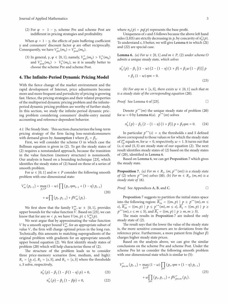
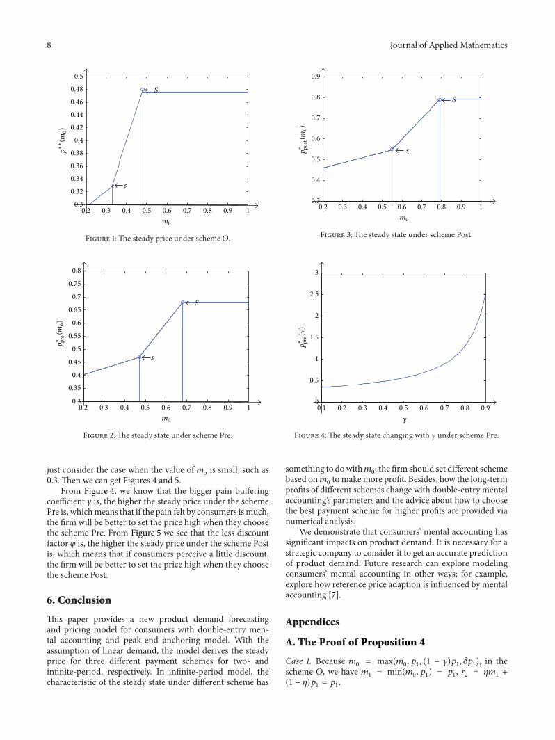
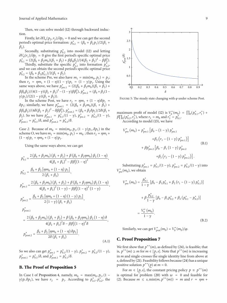