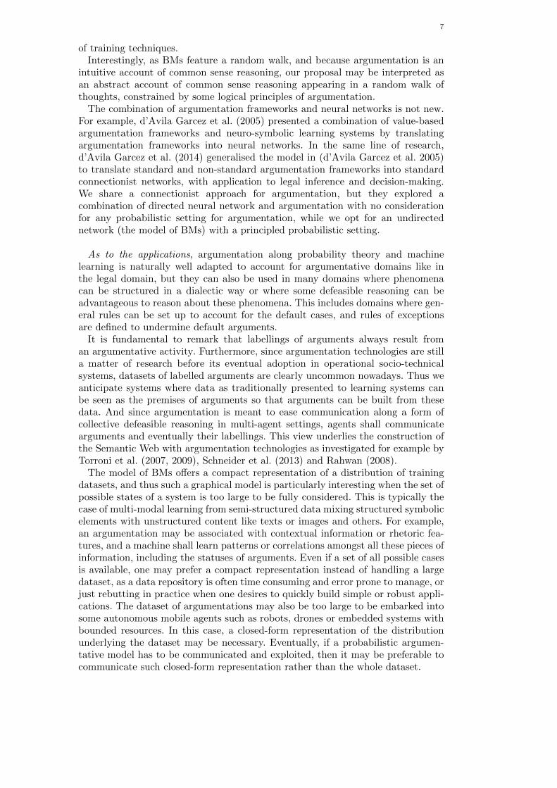
Argument & Computation

RESEARCH ARTICLE

Probabilistic Abstract Argumentation:

an Investigation with Boltzmann Machines.

Regis Rivereta , Dimitrios Korkinofb, Moez Draiefc and Jeremy Pittd

aData61 - CSIRO, Brisbane, Australia; bCortexica Vision Systems, London, United

Kingdom; cHuawei Technologies, Paris, France; dImperial College, London, United

Kingdom

Probabilistic argumentation and neuro-argumentative systems offer new computational per-spectives for the theory and applications of argumentation, but their principled constructioninvolve two entangled problems. On the one hand, probabilistic argumentation aims at com-bining the quantitative uncertainty addressed by probability theory with the qualitative uncer-tainty of argumentation, but probabilistic dependences amongst arguments as well as learningare usually neglected. On the other hand neuro-argumentative systems offer the opportunityto couple the computational advantages of learning and massive parallel computation fromneural networks with argumentative reasoning and explanatory abilities, but the relation ofprobabilistic argumentation frameworks with these systems have been ignored so far. Towardsthe construction of neuro-argumentative systems based on probabilistic argumentation, we as-sociate a model of abstract argumentation and the graphical model of Boltzmann machinesin order to (i) account for probabilistic abstract argumentation with possible and unknownprobabilistic dependences amongst arguments, (ii) learn distributions of labellings from a setof cases and (iii) sample labellings according to the learned distribution. Experiments on do-main independent artificial datasets show that argumentative Boltzmann machines can betrained with conventional training procedures and compare well with conventional machinesfor generating labellings of arguments, with the assurance of generating grounded labellings- on demand.

Keywords: Machine Learning, Probabilistic Argumentation, Graphical Models, BoltzmannMachines, Neuro-argumentative Systems, Product of Experts.

1. Introduction

The combination of formal argumentation and probability theory to obtain formal-isms catering for qualitative uncertainty as well as qualitative uncertainty has at-tracted much attention in the recent years, see, for example, (Dondio 2014, Hunter2013, Li et al. 2011, Sneyers et al. 2013, Thimm 2012), and applications have beensuggested for example in the legal domain by Riveret et al. (2008, 2007), Rothet al. (2007) and Dung and Thang (2010). The underlying argumentation frame-works, the probability interpretation, the probability spaces and the manipulationof probabilities vary due to the different interests (see next section for details),but settings dealing with probabilistically dependent arguments, along issues re-garding the computational complexity of inferences and learning, have been hardlyexplored so far.

However, the pursuit for efficient inference and learning in domains possiblystructured by some logic-based knowledge is not new. For instance, statistical rela-

∗Corresponding author. Email: regis.riveret@nicta.com.au

2

tional learning (SRL) (Getoor and Taskar 2007) is a burgeoning field at the cross-road of statistics, probability theory, logics and machine learning, and a plethoraof frameworks have been proposed, see, for example, Probabilistic Relational Mod-els (Getoor et al. 2007) and Markov Logic Networks (Richardson and Domingos2006). Inspired by these approaches consisting in the combination of logic-basedsystems and graphical models to handle probabilistic dependences, we are willingto investigate the use of graphical models to tackle dependences in a setting ofprobabilistic abstract argumentation.

Another interesting and parallel active line of research possibly combining proba-bility theory, logics and machine learning regards neuro-symbolic systems meant tojoin the strength of neural network models and logics (d’Avila Garcez et al. 2008):neural networks offer sturdy learning with the possibility of massive parallel com-putation, while logic brings intelligible knowledge representation and reasoningwith explanatory ability, thereby facilitating the transmission of learned knowl-edge to other agents. Considering the importance of defeasible reasoning for agentsreasoning with incomplete information and the intuitive account of this type ofreasoning by formal argumentation, neuro-argumentative agents shall provide anergonomic representation and argumentative reasoning aptitude to the underly-ing neural networks. However, such neuro-argumentation has been hardly exploredso far, cf. d’Avila Garcez et al. (2014), and thus we are willing to investigate apossible construction of neuro-argumentative systems with a principled account ofprobabilistic argumentation.Contribution. We investigate an integration of abstract argumentation and

probability theory with undirected graphical models and in particular with thegraphical model of Boltzmann machines (BMs). This combination of argumen-tation and graphical models allows us to relax assumptions on the probabilisticindependences amongst arguments, and to obtain a closed-form representation ofthe distribution underlying observed labellings of arguments. By doing so, we canlearn distributions of labellings from a set of cases (in an unsupervised manner)and sample labellings according to the learned distribution. We focus on genera-tive learning and we thus propose a labelling random walk allowing us to generategrounded labellings with respect to the learned distribution. To make our ideas aswidely applicable as possible, we investigate the use of BMs with the common ab-stract setting for argumentation of Dung (1995) where the content of arguments isleft unspecified, hence we do not deal with structured argumentation in this paper,nor with sub-arguments, see (Riveret et al. 2015) for a development of this paperwhich accounts for sub-arguments.

Since the model of BMs are commonly interpreted as a model of neural networks,we are moving towards the construction of neuro-argumentative systems based ona principled account of probabilistic argumentation. Moreover, as the graphicalmodel of BMs can be also interpreted as a product of experts (PoE), our contribu-tion can also interpreted as a probabilistic model of an assembly of experts judgingthe statuses of arguments in an unanimous manner.

We investigate thus ‘argumentative Boltzmann machines’ meant to learn a func-tion producing a probability distribution over statuses of arguments and to producepossible justified or rejected arguments sampled according to the learned distribu-tion. As proposed by Mozina et al. (2007) and d’Avila Garcez et al. (2014), ar-gumentation appears as a guide to learn hypotheses, that is, some backgroundknowledge is assumed to be encoded into an argumentative structure that shallconstrain the learning and the labelling of argumentative hypotheses. Structurelearning is not addressed in this paper.Outline. The paper is organised as follows. The motivations and possible appli-

3

cations of our proposal are developed in Section 2. The abstract argumentation isintroduced in Section 3. We associate to it a probabilistic setting with a discussionwith respect to probabilistic graphical models in Section 4, and we develop theprobabilistic setting into an energy-based model in Section 5. We overview BMs inSection 6, and we propose ‘argumentative Boltzmann machines’ in Section 7. Wegive some experimental insights in Section 8 before concluding.

2. Motivations and Applications

The first motivation of the present work originates from the observation that in-vestigations into probabilistic argumentation had little consideration for the prob-abilistic dependences amongst arguments and for learning, cf. (Riveret et al. 2012)and (Sneyers et al. 2013).

Roth et al. (2007) used a probabilistic instantiation of an abstract argumentationframework in Defeasible Logic (Governatori et al. 2004), with the focus on deter-mining strategies to maximize the chances of winning legal disputes. In this work,the probability of the defeasible status of a conclusion is the sum of cases where thisstatus is entailed. A case is a set of premises which are assumed independent. Inthe same line of research, Riveret et al. (2007) investigated a probabilistic variantof a rule-based argumentation framework proposed by Prakken and Sartor (1997).They looked at the probability to win a legal dispute, and thus on the probabil-ity that arguments and statements get accepted by an adjudicator. The proposalfocused on the computation of probabilities of justification reflecting moves in adialogue. They emphasized a distinction between the probability of the event of anargument and the probability of justification of an argument. The proposal assumesthe independence amongst premises and arguments so that the probability of anargument is the product of the probability of its premises. Riveret et al. (2012)further developed the setting of Roth et al. (2007) to a rule-based argumentationframework by associating a potential to every sub-theory induced by a larger hypo-thetical theory. The potentials are then learned using reinforcement learning. Ourproposal is inspired by this potential-based model of probabilistic argumentation,but for abstract argumentation combined with energy-based undirected graphicalmodels, and in particular with the graphical model of BMs.

Sneyers et al. (2013) tackled a similar setting of Riveret et al. (2007) (but withoutthe concern of reflecting the structure of dialogues) by defining a probabilistic ar-gumentation logic and implementing it with the language CHRiSM (Sneyers et al.2010), a rule-based probabilistic logic programming language based on ConstraintHandling Rules (CHR) (Fruhwirth 2009) associated with a high-level probabilis-tic programming language called PRISM (Sato 2008); this language must not beconfused with the system PRISM for probabilistic model checking developed byHinton et al. (2006). They discussed how it can be seen as a probabilistic general-ization of the defeasible logic proposed by (Nute 2001), and showed how it providesa method to determine the initial probabilities from a given body of precedents. InCHRiSM, rules have an attached probability and each rule is applied with respectto its probability: rules are probabilistically independent.

Dung and Thang (2010) extended Dung’s abstract argumentation framework byinvestigating a probabilistic assumption-based argumentation (PABA) framework(Bondarenko et al. 1997) for jury-based dispute resolution. Every juror is associ-ated with a probability space where a possible world can be interpreted as a setof arguments. The probability of an argument with respect to a juror and thegrounded semantic is the sum of the probability of the juror’s worlds entailing thisargument. Thus, every juror determines the probability weights of the arguments.

4

The probability space of every juror is further specified by mapping it to a PABAframework where some probabilistic parameters (appearing in some rules) definethe possible worlds.

Li et al. (2011) proposed an extension of Dung (1995)’s framework to build prob-abilistic argumentation frames by associating probabilities with the events of argu-ments and defeats. The sample space is constituted by the possible argumentationsub-graphs induced from a probabilistic argumentation graph. Assuming the inde-pendence of arguments and defeats, the joint probability of the events of argumentsand defeats induced from a probabilistic graph is then defined using the productrule for independent events. The probability of a set of justified arguments is definedas the marginal probability over the sub-graphs justifying this set of arguments.This setting is thus in tune with the setting used by Roth et al. (2007) where theabstract argumentation framework is instantiated in Defeasible Logic (Governatoriet al. 2004) and when the sample space of sub-graphs is mapped to a sample spaceof cases, or with the proposal of Dung and Thang (2010) when the sample spaceof sub-graphs is mapped to the sample space as set of arguments of a juror. Li atal. proposed to tackle the exponential complexity of the sample space by a Monte-Carlo algorithm to approximate the probability of a set of justified arguments,arguments being assumed independent. Li developed her work, see (Li 2015), toaccount for dependences amongst arguments when they share the same premises,however these dependences remain logic and not probabilistic.

The abstract setting of Li et al. (2011) was followed by several investigations. Forexample, Fazzinga et al. (2013) observed that the Monte-Carlo techniques proposedby Li et al. (2011) can be improved, and they showed that computing the proba-bility that a set of arguments is a set of justified arguments is either PTIME orFP#P -complete depending on the semantics. In a similar line of research, Dondio(2014) tackled the complexity of the sample space of the probabilistic frameworkproposed in (Li et al. 2011) by investigating a recursive algorithm to compute theprobability of acceptance of each argument under grounded and preferred seman-tics. The underlying assumptions are that the probability of every argumentationsub-graph is known, or that the arguments are probabilistically independent, orthat the premises are independent as in (Riveret et al. 2007).

Another view on probabilistic argumentation focuses on an interpretation ofprobabilities as subjective probabilities meant to represent the degree to which anargument is believed to hold. For example, Hunter (2013) developed the idea of aprobability value attached to every argument, and investigated this idea for argu-ments that are constructed using classical logic. Then various kinds of inconsistencyarising within the framework are studied. Thimm (2012) also focused on an inter-pretation of probabilities as subjective probabilities, and investigated probabilityfunctions that agree with some intuitions about the interrelationships of argumentsand attacks. In these views, instead of differentiating the probability of the eventof an argument and the probability of the justification of this argument, the prob-ability of an argument is interpreted as its probability of its justification status.Hunter and Thimm (2014) further consolidated this interpretation according towhich the statuses of arguments can be labelled in a similar way than conventionalformal argumentation by assuming some constraints on arguments probabilities.Baroni et al. (2014) observed that, though Hunter and Thimm focused on an in-terpretation of probabilities as subjective probabilities, Hunter and Thimm usedKolmogorov axioms instead of a probability theory more akin to a subjective prob-ability setting. For this reason, Baroni et al. advocated and used the theory ofDe Finetti (1974) for an epistemic approach similar to (Hunter 2013) and (Thimm2012).

5

In this paper, we favour a frequentist interpretation of probabilities, instead of aninterpretation of probabilities as subjective probabilities. The subjective approachis interesting when the domain is small and when objectivity is not important, buta frequentist approach where probabilities are statically computed or learned iscertainly more appropriate for larger domains or more objective measures. How-ever, since frequency ratios may also be interpreted in subjective probabilities andvice versa, we do not discard an interpretation of probabilities as subjective prob-abilities for our framework, in particular when the framework is understood fromthe perspective of the model of PoE.

Whatever the interpretation of probabilities, we note that the extraction of prob-ability measures is rather neglected in the above proposals and there is no consider-ation for learning. An exception is the work by Sneyers et al. (2013) which proposesa solution to determine the initial probabilities from a given body of precedents(but rules are probabilistically independent). Riveret et al. (2012) also investigatedan approach using reinforcement learning to learn the optimal probability of usingsome arguments by an agent.

Furthermore, we also note that all the above works assume that either the prob-ability of every argumentation sub-graph is known (for theoretical purposes) orthat the arguments are probabilistically independent (for practical purposes), butsuch assumptions may not hold in the general case and for many applications. Forthese reasons, we aim at developing a computational probabilistic argumentationframework able to handle probabilistic dependences amongst arguments and learnprobability measures from examples.

The second motivation of our proposal stems from the observation that log-ics, principled probabilistic and statistical approaches along machine learning havebeen largely studied to learn from uncertain knowledge and to perform inferenceswith this knowledge. In particular, statistical relational learning (SRL) (Getoorand Taskar 2007) is the field at this crossroad, with successful integrations, seee.g. Probabilistic Relational Models (Getoor et al. 2007) and Markov Logic Net-works (Richardson and Domingos 2006). In these approaches, logics are used tostructure in a qualitative manner the probabilistic relations amongst entities. Typ-ically, (a subset of) first-order logic formally represents a qualitative knowledgedescribing the structure of a domain in a general manner (using universal quan-tification) while techniques from graphical models (Koller and Friedman 2009),such as Bayesian networks (Getoor et al. 2007) or Markov networks (Richardsonand Domingos 2006), are applied to handle probability measures on the structuredentities. Though SRL approaches focus on capturing data in its relational formand we are only dealing with an abstract and flat data representation (inducedby our setting of abstract argumentation), we are inspired by these approachesconsisting in combinations of graphical models and logic-based systems, and wepropose that investigations for probabilistic argumentation shall benefit from theuse of graphical models too.

In this paper we will focus on abstract argumentation, and thus we need to selecta probabilistic graphical model appropriate for our purposes. In SRL systems, theprobabilistic dependences are usually represented by the graphical structure of theprobabilistic graphical model associated with the logic-based knowledge. These re-lations of (in)dependence amongst entities of the system are specified or induced bythe logic-based knowledge, or given by domain experts or learned from examples.In the case of probabilistic argumentation, though arguments are usually assumedto have no other dependence relations other than the relations of attacks and even-tual supports, we will argue that the argumentative structure and the probabilistic

6

structure have to be separated (see Section 4). We will assume that the dependencesare not specified (from a human operator for instance): so we will focus on the par-ticular class of graphical models of BMs where any dependence amongst argumentsis possible. These machines are a Monte Carlo version of Hopfield networks inspiredby models in statistical physics, and they can be interpreted as a special case ofPoE or Markov networks (see Section 6). The model of BMs appears thus as anappealing theoretical model which has shown to be useful for practical problemsand which paves the way to some multi-modal machines (combining audio, videoand symbolic modes for example), but this model has not been considered so farto tackle probabilistic and learning settings of formal argumentation.

Learning is commonly approached in a discriminative or a generative way. Thedifference holds in that a generative approach deals with the joint probabilityover all variables in a system and handles it to perform other tasks like classifica-tion, while discriminative approaches are meant to directly capture the conditionalprobability for classification. More precisely, if a system is featured by N variables(x1, . . . , xN ), the generative approach will account for the full joint distributionp(x1, . . . , xN ), while the discriminative approach will attempt to capture a con-ditional probability like p(xN |x1, . . . , xN−1) where xN is a classifying variable. Agenerative model can be handled to deal with tasks performed by discriminativeapproaches, or it can be used in straightforward manner to simulate (that is, gen-erate or sample) configurations of a system. In this paper, we will focus on thegenerative approach. So, given examples of the form (x1, . . . , xN ), we will train anargumentative BM to account for the full joint distribution p(x1, . . . , xN ) of the ex-amples in a generative manner, paving the way to the manipulation of the learnedjoint distribution to account for a conditional distribution. Since we are interestedby generative learning, we will focus on a labelling random walk which allows usto generate grounded labellings according to a learned probability distribution.

Whilst training datasets in state-of-the-art SRL systems are normally relational,a training example for BMs is typically a binary vector. For our purposes and sincewe are dealing with abstract argumentation, a training case will be a labelling ofa set of arguments, that is, every argument will be associated a label to indicatewhether its status is justified, rejected, undecided or unexpressed. We will showthat the space complexity of the sample space for probabilistic argumentation canbe dramatically reduced when using BMs, and a compact model can be learned atrun time while producing labellings.

The third motivation of our work regards the construction of neuro-symbolicagents. Neuro-symbolic agents join the strength of neural networks and logics(d’Avila Garcez et al. 2008). Neural networks offer robust learning with the possi-bility of massive parallel computation and have successfully shown to grasp in-formation and uncertainty where symbolic approaches failed. However, as net-works suffer from their ‘black box’ nature, logic formalisms shall bring intelligibleknowledge representation and reasoning into the networks with explanatory ability,thereby facilitating the transmission of learned knowledge to other agents.

As artificial neural networks are inspired by natural nervous systems, we proposeto associate with them argumentation as a natural account of human defeasiblereasoning. Neuro-argumentative agents shall provide an ergonomic representationand argumentative reasoning aptitude to the underlying neural networks and easeits possible combination with some argumentative agent communication languages.We will propose to build neuro-symbolic agents based on BMs and formal argu-mentation. As different Monte Carlo sampling approaches to Boltzmann machinesare possible, we will propose a sampling of labellings allowing the use of variants

7

of training techniques.Interestingly, as BMs feature a random walk, and because argumentation is an

intuitive account of common sense reasoning, our proposal may be interpreted asan abstract account of common sense reasoning appearing in a random walk ofthoughts, constrained by some logical principles of argumentation.

The combination of argumentation frameworks and neural networks is not new.For example, d’Avila Garcez et al. (2005) presented a combination of value-basedargumentation frameworks and neuro-symbolic learning systems by translatingargumentation frameworks into neural networks. In the same line of research,d’Avila Garcez et al. (2014) generalised the model in (d’Avila Garcez et al. 2005)to translate standard and non-standard argumentation frameworks into standardconnectionist networks, with application to legal inference and decision-making.We share a connectionist approach for argumentation, but they explored acombination of directed neural network and argumentation with no considerationfor any probabilistic setting for argumentation, while we opt for an undirectednetwork (the model of BMs) with a principled probabilistic setting.

As to the applications, argumentation along probability theory and machinelearning is naturally well adapted to account for argumentative domains like inthe legal domain, but they can also be used in many domains where phenomenacan be structured in a dialectic way or where some defeasible reasoning can beadvantageous to reason about these phenomena. This includes domains where gen-eral rules can be set up to account for the default cases, and rules of exceptionsare defined to undermine default arguments.

It is fundamental to remark that labellings of arguments always result froman argumentative activity. Furthermore, since argumentation technologies are stilla matter of research before its eventual adoption in operational socio-technicalsystems, datasets of labelled arguments are clearly uncommon nowadays. Thus weanticipate systems where data as traditionally presented to learning systems canbe seen as the premises of arguments so that arguments can be built from thesedata. And since argumentation is meant to ease communication along a form ofcollective defeasible reasoning in multi-agent settings, agents shall communicatearguments and eventually their labellings. This view underlies the construction ofthe Semantic Web with argumentation technologies as investigated for example byTorroni et al. (2007, 2009), Schneider et al. (2013) and Rahwan (2008).

The model of BMs offers a compact representation of a distribution of trainingdatasets, and thus such a graphical model is particularly interesting when the set ofpossible states of a system is too large to be fully considered. This is typically thecase of multi-modal learning from semi-structured data mixing structured symbolicelements with unstructured content like texts or images and others. For example,an argumentation may be associated with contextual information or rhetoric fea-tures, and a machine shall learn patterns or correlations amongst all these pieces ofinformation, including the statuses of arguments. Even if a set of all possible casesis available, one may prefer a compact representation instead of handling a largedataset, as a data repository is often time consuming and error prone to manage, orjust rebutting in practice when one desires to quickly build simple or robust appli-cations. The dataset of argumentations may also be too large to be embarked intosome autonomous mobile agents such as robots, drones or embedded systems withbounded resources. In this case, a closed-form representation of the distributionunderlying the dataset may be necessary. Eventually, if a probabilistic argumen-tative model has to be communicated and exploited, then it may be preferable tocommunicate such closed-form representation rather than the whole dataset.

8

In multi-agent simulations, stochastic behaviours of heterogeneous agentsmay be simulated by sampling behaviours from argumentative machines, whereargumentation shall provide scrutiny on the simulated behaviours. As somenon-monotonic logics instantiating Dung’s abstract argumentation frameworkare proposed to model normative multi-agent systems (see e.g. Governatoriet al. (2005), Sartor (2005)) with some implementations (Riveret et al. 2012)), themodel of BMs combined with abstract argumentation paves the way to simulationscombining neural agents and institutions. In ‘living’ simulators for which datashall be streamed into (see e.g. Paolucci et al. (2013)), a compact model shall belearned ‘on the fly’ while producing possible labellings sampled according to thelearned distribution. More generally, learning a compact model on the fly whilesampling labellings can also be interesting for so-called complex event processingsystems capturing data streams.

3. Abstract Argumentation Framework

In this section, we introduce our abstract argumentation framework. We begin withthe definition of an argumentation graph following Dung (1995).

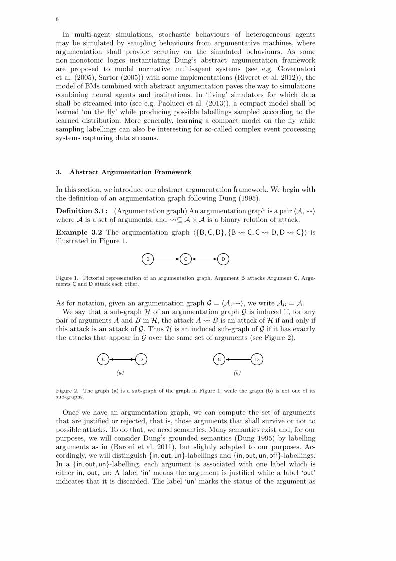
Definition 3.1: (Argumentation graph) An argumentation graph is a pair 〈A, 〉where A is a set of arguments, and ⊆ A×A is a binary relation of attack.

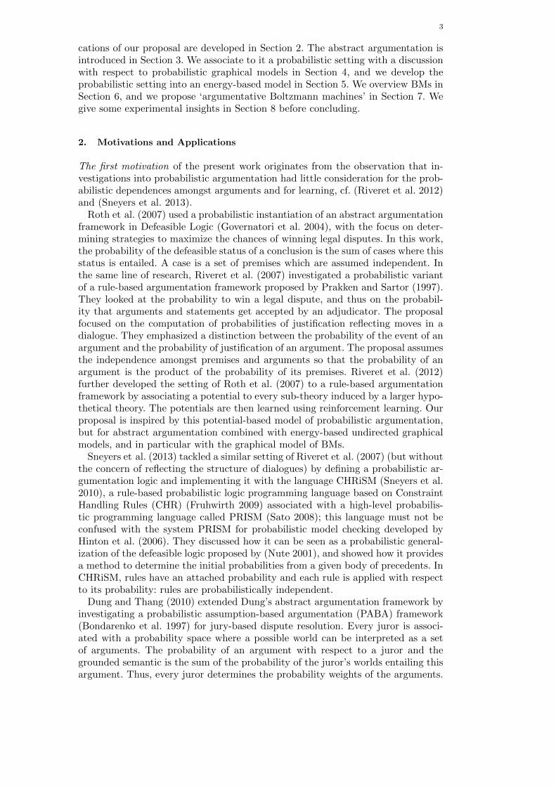
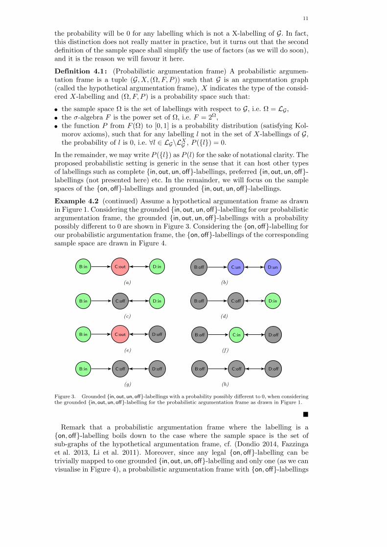
Example 3.2 The argumentation graph 〈B,C,D, B C,C D,D C〉 isillustrated in Figure 1.

B C D

Figure 1. Pictorial representation of an argumentation graph. Argument B attacks Argument C, Argu-ments C and D attack each other.

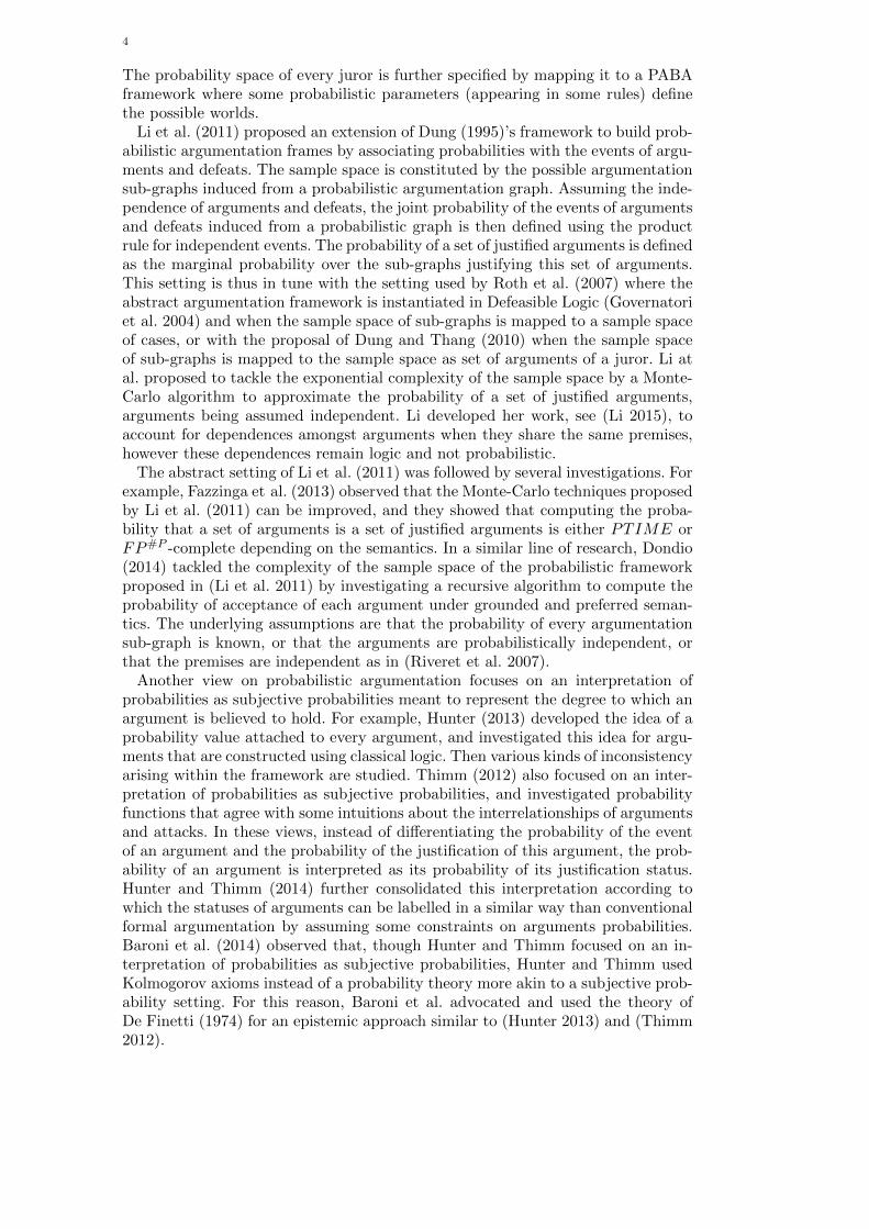
As for notation, given an argumentation graph G = 〈A, 〉, we write AG = A.We say that a sub-graph H of an argumentation graph G is induced if, for any

pair of arguments A and B in H, the attack A B is an attack of H if and only ifthis attack is an attack of G. Thus H is an induced sub-graph of G if it has exactlythe attacks that appear in G over the same set of arguments (see Figure 2).

C D

(a)

C D

(b)

Figure 2. The graph (a) is a sub-graph of the graph in Figure 1, while the graph (b) is not one of itssub-graphs.

Once we have an argumentation graph, we can compute the set of argumentsthat are justified or rejected, that is, those arguments that shall survive or not topossible attacks. To do that, we need semantics. Many semantics exist and, for ourpurposes, we will consider Dung’s grounded semantics (Dung 1995) by labellingarguments as in (Baroni et al. 2011), but slightly adapted to our purposes. Ac-cordingly, we will distinguish in, out, un-labellings and in, out, un, off-labellings.In a in, out, un-labelling, each argument is associated with one label which iseither in, out, un: A label ‘in’ means the argument is justified while a label ‘out’indicates that it is discarded. The label ‘un’ marks the status of the argument as

9

undecided. We introduce two novel labels: ‘on’ and ‘off’ to indicate whether anargument is expressed or not. We say that an argument is expressed if it is labelledon, or either in, out or un, otherwise it is not expressed, that is, it is labelled off.So, in a on, off-labelling or in a in, out, un, off-labelling, the label ‘off’ indicatesthat the argument is not expressed.

Definition 3.3: (Labellings) Let G be an argumentation graph.

• A on, off-labelling of G is a total function l : AG → on, off.• A in, out, un-labelling of G is a total function l : AG → in, out, un.• A in, out, un, off-labelling of G is a total function l : AG → in, out, un, off.

Notice that the labelling functions are denoted with a lower case, reserving theupper case to denote random labellings in the probabilistic setting (as we will seein Section 4). We write in(l) for A|l(A) = in, out(l) for A|l(A) = out, un(l) forA|l(A) = un, on(l) for A|l(A) = on and off(l) for A|l(A) = off. In the re-mainder, a in, out, un-labelling l will be represented as a tuple (in(l), out(l), un(l)),and a in, out, un, off-labelling l as a tuple (in(l), out(l), un(l), off(l)). Next completelabellings are defined by constraints amongst the labels in and out.

Definition 3.4: (Complete in, out, un-labelling) Let G be an argumentationgraph, a complete in, out, un-labelling of G is a in, out, un-labelling such thatfor every argument A in AG it holds that:

• A is labelled in if, and only if, all attackers of A are labelled out,• A is labelled out if, and only if, A has an attacker that is labelled in.

An argumentation graph may have several complete in, out, un-labellings.Given a graph, we will focus in the remainder on the unique complete labellingwith the smallest set of labels in (or equivalently the largest set of labels un) (Ba-roni et al. 2011, Dung 1995).

Definition 3.5: (Grounded in, out, un-labelling) Let G be an argumentationgraph and l a complete in, out, un-labelling of G. A labelling l is a groundedin, out, un-labelling of G if in(l) is minimal (w.r.t. set inclusion) amongst all com-plete in, out, un-labellings of G.

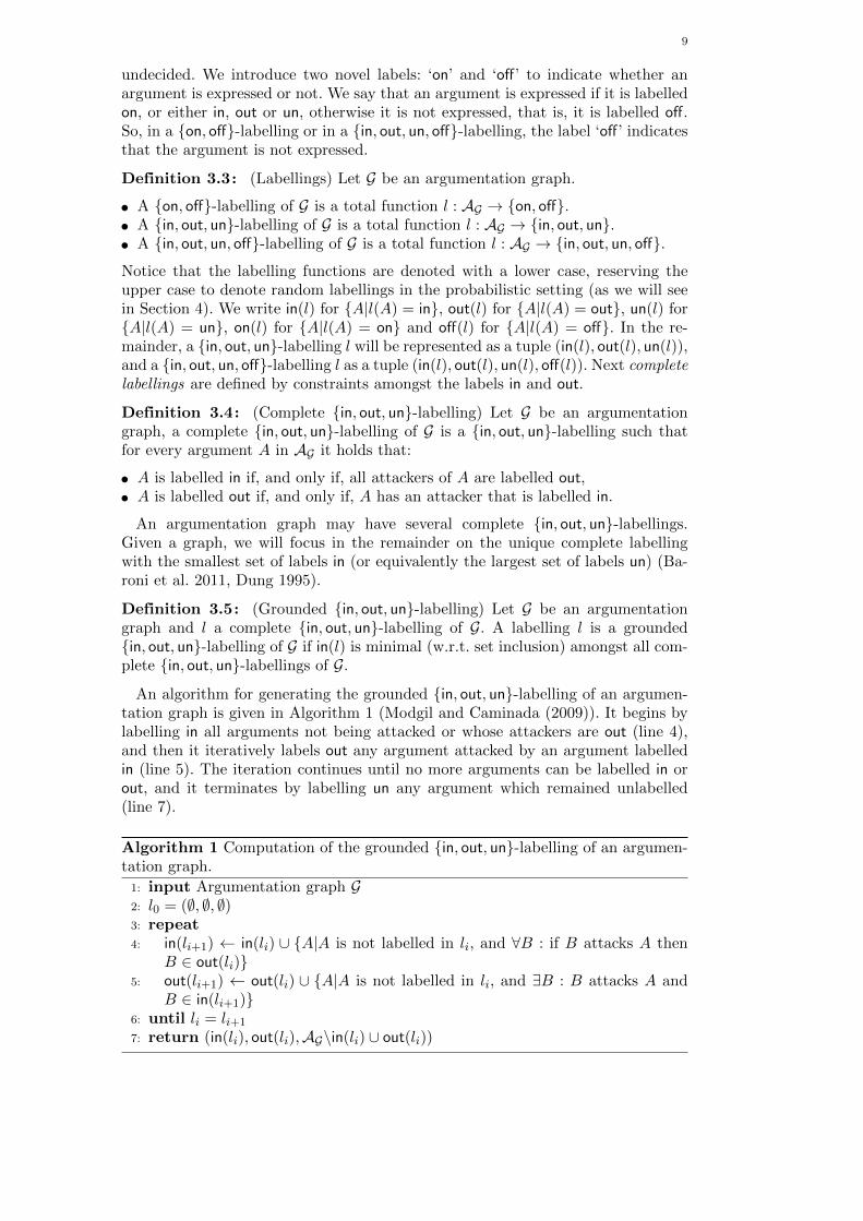
An algorithm for generating the grounded in, out, un-labelling of an argumen-tation graph is given in Algorithm 1 (Modgil and Caminada (2009)). It begins bylabelling in all arguments not being attacked or whose attackers are out (line 4),and then it iteratively labels out any argument attacked by an argument labelledin (line 5). The iteration continues until no more arguments can be labelled in orout, and it terminates by labelling un any argument which remained unlabelled(line 7).

Algorithm 1 Computation of the grounded in, out, un-labelling of an argumen-tation graph.

1: input Argumentation graph G2: l0 = (∅, ∅, ∅)3: repeat4: in(li+1) ← in(li) ∪ A|A is not labelled in li, and ∀B : if B attacks A then

B ∈ out(li)5: out(li+1) ← out(li) ∪ A|A is not labelled in li, and ∃B : B attacks A and

B ∈ in(li+1)6: until li = li+1

7: return (in(li), out(li),AG\in(li) ∪ out(li))

10

This algorithm is sound because the resulting in, out, un-labelling l is completeand in(l) is minimal, thus the labelling l is a grounded in, out, un-labelling.At each iteration, one argument at least is labelled, otherwise the algorithmterminates. Therefore, when the input is a graph of N arguments, then there isnecessarily less than N iterations. For each iteration, the status of N argumentshas to be checked with respect to the status of N arguments in the worst case.Consequently, the time complexity of Algorithm 1 is polynomial in the worst case.

We introduced in, out, un, off-labellings in Definition 3.3 by extending the com-mon in, out, un-labelling with unexpressed arguments, we present now groundedin, out, un, off-labellings. The substantial underlying idea is that only expressedarguments can be refuted, and only expressed arguments can effectively attackother arguments.

Definition 3.6: (Grounded in, out, un, off-labelling) Let G be an argumentationgraph and H an induced sub-graph of G. A grounded in, out, un, off-labelling ofG is a in, out, un, off-labelling such that:

• every argument inAH is labelled according to the grounded in, out, un-labellingof H,

• every argument in AG\AH is labelled off.

An argumentation graph has a unique grounded in, out, un-labelling, but ithas as many grounded in, out, un, off-labellings as sub-graphs. See Figure 3 forexamples of grounded in, out, un, off-labellings.

As for notational matters, the sets of labellings of an argumentation graphG will be denoted LG . A complete in, out, un, off-labelling will be abbrevi-ated as in, out, un, offc-labelling, and a grounded in, out, un, off-labelling asin, out, un, offg-labelling. By doing so, we can denote the set of X-labellings ofa graph G as LXG , and each set will basically constitute a sample space of ourprobabilistic setting for argumentation. Considering a X-labelling, if a labellingof arguments is not a X-labelling, then it is an illegal labelling, else it is a legallabelling.

4. Probabilistic Abstract Argumentation Framework

In this section, we introduce our probabilistic setting for the abstract argumenta-tion framework as given in the previous section. Notice that there are many waysto define the probability space of a setting for probabilistic argumentation and thechoice of a probability space shall be made in function of the envisaged applica-tions. Our choice was conducted by the promotion of simplicity and to match ouruse of the graphical model of BMs for probabilistic argumentation towards theconstruction of neuro-argumentative systems.

So for our purposes, we define a sample space as the set of labellings of ahypothetical argumentation frame (or simply called a hypothetical frame) whichis an argumentation graph. Now, when building a probabilistic setting, we haveto make the distinction between an impossible event (that is, the event does notbelong to the sample space), and an event with probability 0. Similarly, given ahypothetical argumentation frame G and a X-labelling (e.g. a on, off-labelling ora grounded in, out, un, off-labelling or any other in, out, un, off-labelling), thereis the choice between either (i) defining the sample space as the set of the X-labellings of G, or (ii) defining the sample space as the set of any labelling of G and

11

the probability will be 0 for any labelling which is not a X-labelling of G. In fact,this distinction does not really matter in practice, but it turns out that the seconddefinition of the sample space shall simplify the use of factors (as we will do soon),and it is the reason we will favour it here.

Definition 4.1: (Probabilistic argumentation frame) A probabilistic argumen-tation frame is a tuple (G, X, (Ω, F, P )) such that G is an argumentation graph(called the hypothetical argumentation frame), X indicates the type of the consid-ered X-labelling and (Ω, F, P ) is a probability space such that:

• the sample space Ω is the set of labellings with respect to G, i.e. Ω = LG ,

• the σ-algebra F is the power set of Ω, i.e. F = 2Ω,

• the function P from F (Ω) to [0, 1] is a probability distribution (satisfying Kol-morov axioms), such that for any labelling l not in the set of X-labellings of G,the probability of l is 0, i.e. ∀l ∈ LG\LXG , P (l) = 0.

In the remainder, we may write P (l) as P (l) for the sake of notational clarity. Theproposed probabilistic setting is generic in the sense that it can host other typesof labellings such as complete in, out, un, off-labellings, preferred in, out, un, off-labellings (not presented here) etc. In the remainder, we will focus on the samplespaces of the on, off-labellings and grounded in, out, un, off-labellings.

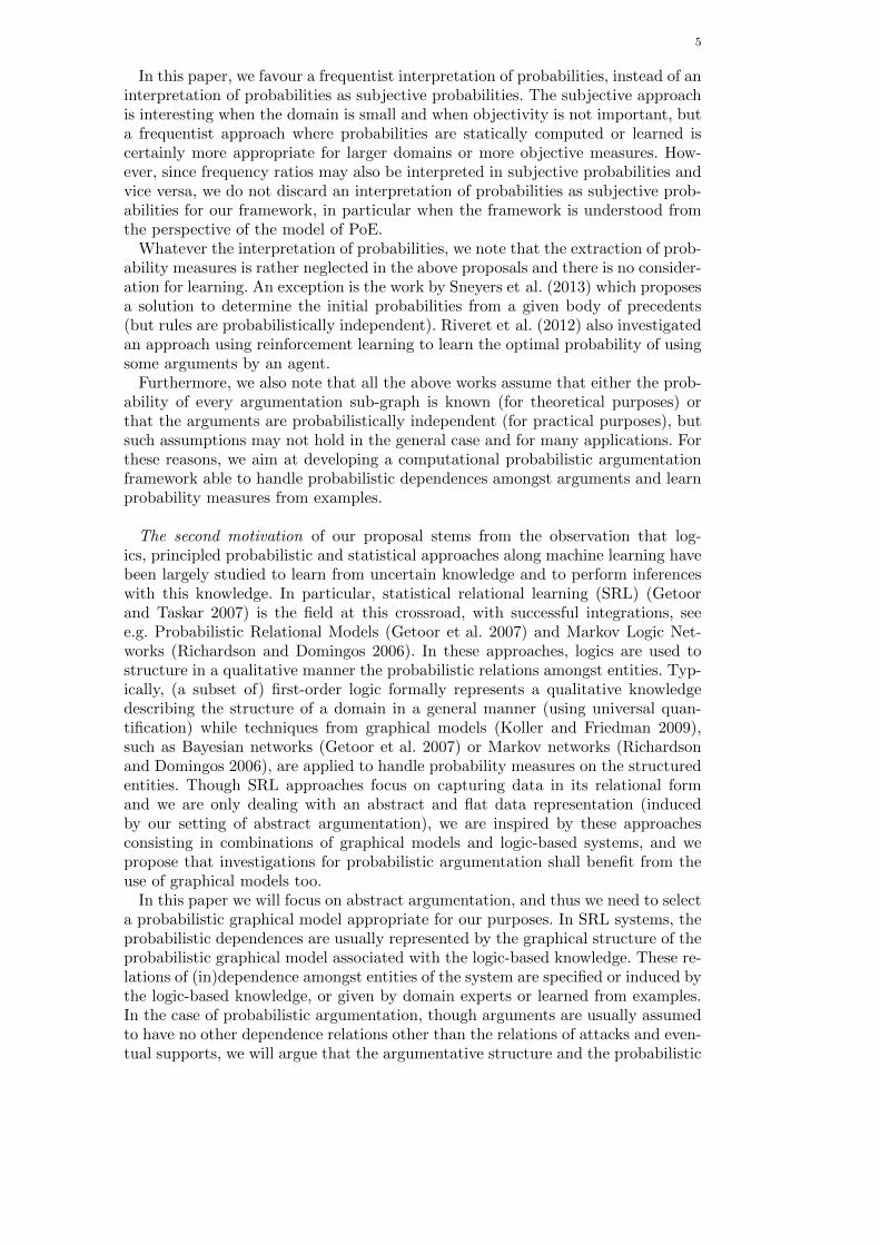
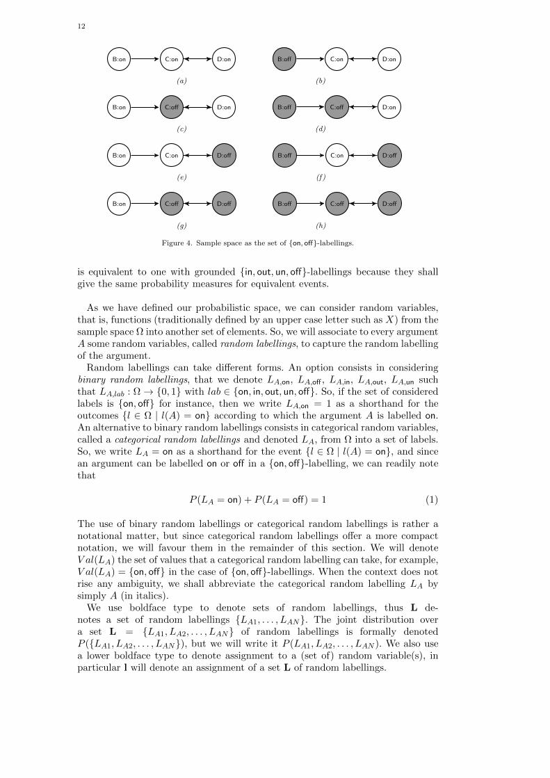
Example 4.2 (continued) Assume a hypothetical argumentation frame as drawnin Figure 1. Considering the grounded in, out, un, off-labelling for our probabilisticargumentation frame, the grounded in, out, un, off-labellings with a probabilitypossibly different to 0 are shown in Figure 3. Considering the on, off-labelling forour probabilistic argumentation frame, the on, off-labellings of the correspondingsample space are drawn in Figure 4.

B:in C:out D:in

(a)

B:off C:un D:un

(b)

B:in C:off D:in

(c)

B:off C:off D:in

(d)

B:in C:out D:off

(e)

B:off C:in D:off

(f)

B:in C:off D:off

(g)

B:off C:off D:off

(h)

Figure 3. Grounded in, out, un, off-labellings with a probability possibly different to 0, when consideringthe grounded in, out, un, off-labelling for the probabilistic argumentation frame as drawn in Figure 1.

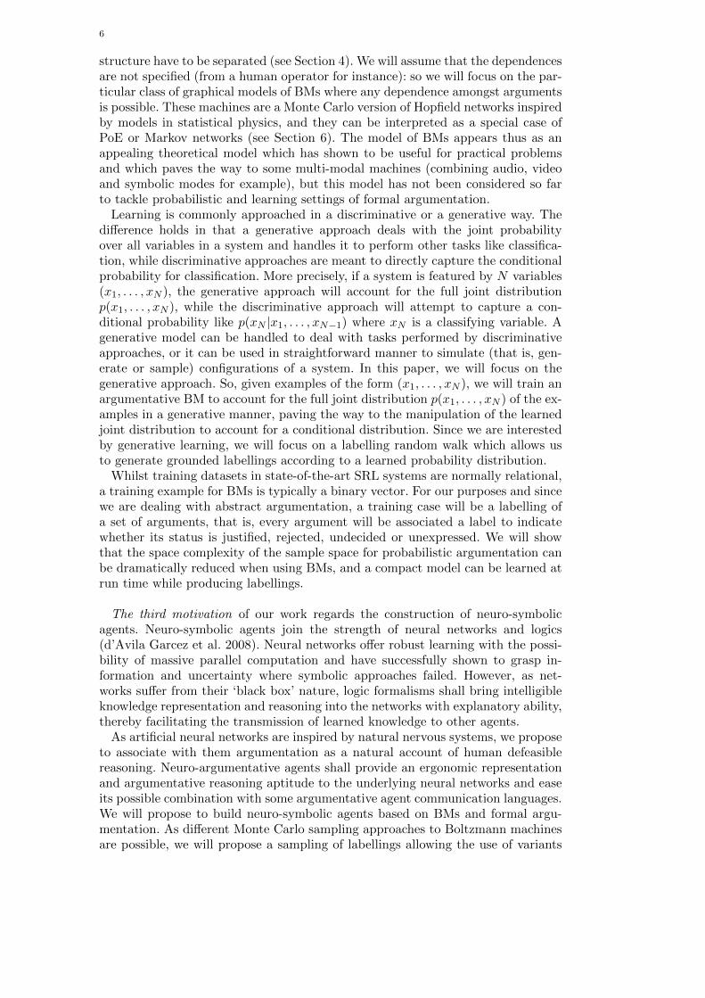
Remark that a probabilistic argumentation frame where the labelling is aon, off-labelling boils down to the case where the sample space is the set ofsub-graphs of the hypothetical argumentation frame, cf. (Dondio 2014, Fazzingaet al. 2013, Li et al. 2011). Moreover, since any legal on, off-labelling can betrivially mapped to one grounded in, out, un, off-labelling and only one (as we canvisualise in Figure 4), a probabilistic argumentation frame with on, off-labellings

12

B:on C:on D:on

(a)

B:off C:on D:on

(b)

B:on C:off D:on

(c)

B:off C:off D:on

(d)

B:on C:on D:off

(e)

B:off C:on D:off

(f)

B:on C:off D:off

(g)

B:off C:off D:off

(h)

Figure 4. Sample space as the set of on, off-labellings.

is equivalent to one with grounded in, out, un, off-labellings because they shallgive the same probability measures for equivalent events.

As we have defined our probabilistic space, we can consider random variables,that is, functions (traditionally defined by an upper case letter such as X) from thesample space Ω into another set of elements. So, we will associate to every argumentA some random variables, called random labellings, to capture the random labellingof the argument.

Random labellings can take different forms. An option consists in consideringbinary random labellings, that we denote LA,on, LA,off , LA,in, LA,out, LA,un suchthat LA,lab : Ω→ 0, 1 with lab ∈ on, in, out, un, off. So, if the set of consideredlabels is on, off for instance, then we write LA,on = 1 as a shorthand for theoutcomes l ∈ Ω | l(A) = on according to which the argument A is labelled on.An alternative to binary random labellings consists in categorical random variables,called a categorical random labellings and denoted LA, from Ω into a set of labels.So, we write LA = on as a shorthand for the event l ∈ Ω | l(A) = on, and sincean argument can be labelled on or off in a on, off-labelling, we can readily notethat

P (LA = on) + P (LA = off) = 1 (1)

The use of binary random labellings or categorical random labellings is rather anotational matter, but since categorical random labellings offer a more compactnotation, we will favour them in the remainder of this section. We will denoteV al(LA) the set of values that a categorical random labelling can take, for example,V al(LA) = on, off in the case of on, off-labellings. When the context does notrise any ambiguity, we shall abbreviate the categorical random labelling LA bysimply A (in italics).

We use boldface type to denote sets of random labellings, thus L de-notes a set of random labellings LA1, . . . , LAN. The joint distribution overa set L = LA1, LA2, . . . , LAN of random labellings is formally denotedP (LA1, LA2, . . . , LAN), but we will write it P (LA1, LA2, . . . , LAN ). We also usea lower boldface type to denote assignment to a (set of) random variable(s), inparticular l will denote an assignment of a set L of random labellings.

13

Given a set L of random labellings, we consider the standard definition of afactor as a function, denoted φ, from the possible set of assignments V al(L) tostrictly positive real numbers R+. The set L is called the scope of the factor φ. Onthis basis, we write the joint distribution of random labellings LA1, . . . , LAN as adistribution parametrised by a set of factors Φ = φ1(L1), . . . , φK(LK):

PΦ(LA1, LA2, . . . , LAN ) =

∏i φi(Li)

ZΦ(2)

where ZΦ is normalising the distribution:

ZΦ =∑

LA1,...,LAN

∏i

φi(Li) (3)

A factor can be thought as an expert putting some credits on assignments, we willreturn on this point when introducing BMs in Section 6.

If the scope of a factor contains two random labellings, then there is a direct prob-abilistic influence between these two random labellings. In this view, it is commonto visualise dependences by relating a factorisation with a graphical structure,typically such as a Markov random field (MRF), also known as Markov network,where nodes represent random variables and arcs indicate dependences amongstthese variables: in this case, a distribution PΦ with Φ = φ1(L1), . . . , φK(LK)factorises over a Markov network H if each Li is a complete sub-graph of H.

It is also common to visualise the factorisation under the graphical model offactor graphs, which is an alternative to Markov networks to explicit the fac-torisation. In this perspective, a factor graph for a set of random labellingsL = (L1, L2, . . . , LN ) and a set of factor functions φ1, . . . , φK is a bipartite graphon a set of nodes corresponding to the variables, and a set of nodes correspondingto the functions. Each function depends on a subset of the variables, and the cor-responding function node is connected to the nodes corresponding to the subsetof variables, that is, if φk depends on Ln, there is an edge connecting the nodesrepresenting φk and Ln.

Example 4.3 Consider an argumentation graph G with five arguments, sayAG = B,C,D,E,F (the attack relation does not matter for our purposes), wecan (arbitrarily) decompose the joint distribution of random labelling in two fac-tors as follows:

P (LB, LC, LD, LE, LF) =φ1(LB, LC, LD) · φ2(LD, LE, LF)

ZΦ(4)

Suppose that the factors take their values as given in the tables of Figure 5.

LB LC LD φ1(LB, LC, LD)on on on 1on on off 100on off on 10on off off 10off on on 50off on off 1off off on 1off off off 1

LD LE LF φ2(LD, LE, LF)on on on 500on on off 100on off on 10on off off 10off on on 50off on off 1off off on 1off off off 1

Figure 5. Tables corresponding to the factors φ1(LB, LC, LD) and φ2(LD, LE, LF).

14

From the given factors, we can compute the joint probability of any on, off-labelling of the argumentation graph. For example, consider the probability of theon, off-labelling where all the arguments are labelled on. Since φ1(LB = on, LC =on, LD = on) = 0 and φ2(LD = on, LE = on, LF = on) = 50, we can compute thefollowing joint probability (amongst others):

P (LB = on, LC = on, LD = on, LE = on, LF = on) ≈ 0 (5)

Graphical models provide a compact and graphical representation of dependencesto deal with joint probability distributions. For example in MRFs, two sets of nodesA and B are conditionally independent given a third set C, if all paths between thenodes in A and B are separated by a node in C. In graphical models, arcs are thusmeant to represent assumptions on conditional independence relationships amongstvariables, and on the basis of these assumptions joint probability can break downinto manageable products of conditional probabilities.

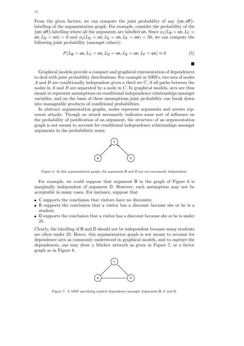
In abstract argumentation graphs, nodes represent arguments and arrows rep-resent attacks. Though an attack necessarily indicates some sort of influence onthe probability of justification of an argument, the structure of an argumentationgraph is not meant to account for conditional independence relationships amongstarguments in the probabilistic sense.

B

C

D

Figure 6. In this argumentation graph, the arguments B and D are not necessarily independent.

For example, we could suppose that argument B in the graph of Figure 6 ismarginally independent of argument D. However, such assumption may not beacceptable in many cases. For instance, suppose that

• C supports the conclusion that visitors have no discounts;

• B supports the conclusion that a visitor has a discount because she or he is astudent;

• D supports the conclusion that a visitor has a discount because she or he is under25.

Clearly, the labelling of B and D should not be independent because many studentsare often under 25. Hence, this argumentation graph is not meant to account fordependence arcs as commonly understood in graphical models, and to capture thedependences, one may draw a Markov network as given in Figure 7, or a factorgraph as in Figure 8.

B

C

D

Figure 7. A MRF specifying explicit dependence amongst Arguments B, C and D.

15

C

φ

B D

Figure 8. A (trivial) factor graph specifying the joint probability P (LB, LC, LD).

This example may be considered in a modified setting for abstract argumentationwith some support relations, see e.g. (Cayrol and Lagasquie-Schiex 2013), so thatarguments B and C are related by some support relations, specifying so someprobabilistic dependences. In this view, we might induce a Markov network froman argumentation graph to capture the probabilistic dependences among the labelsof arguments, but this matter is not addressed in this paper.

In this paper we consider that graphs of probabilistic graphical models and ar-gumentation graphs (and logical structures in general) are not meant to encodethe same type of information (cf. Richardson and Domingos (2006)): graphs ofprobabilistic graphical models encode probabilistic dependence relations, while ar-gumentation graphs encode logic constraints on the possible labellings amongstarguments. In this view, though graphs of probabilistic graphical models and ar-gumentation carry distinct information, we see them as complementary, and anargumentation graph shall be associated with a probabilistic graphical model tospecify probabilistic dependences.

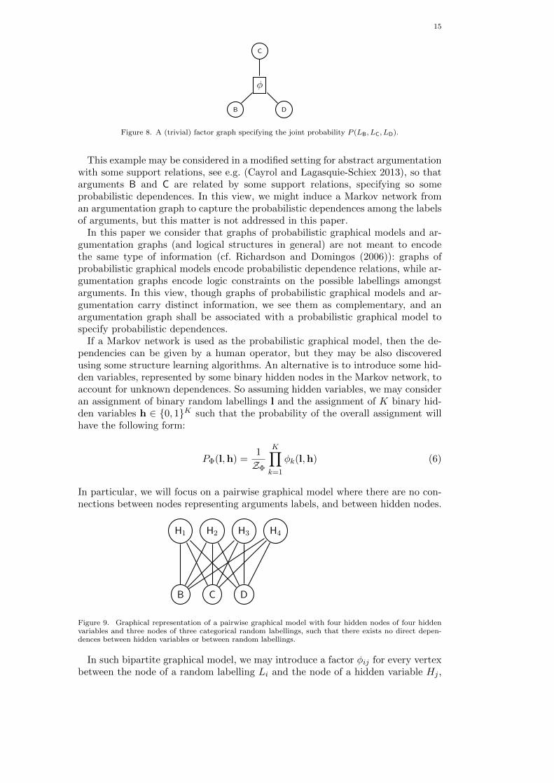
If a Markov network is used as the probabilistic graphical model, then the de-pendencies can be given by a human operator, but they may be also discoveredusing some structure learning algorithms. An alternative is to introduce some hid-den variables, represented by some binary hidden nodes in the Markov network, toaccount for unknown dependences. So assuming hidden variables, we may consideran assignment of binary random labellings l and the assignment of K binary hid-den variables h ∈ 0, 1K such that the probability of the overall assignment willhave the following form:

PΦ(l,h) =1

ZΦ

K∏k=1

φk(l,h) (6)

In particular, we will focus on a pairwise graphical model where there are no con-nections between nodes representing arguments labels, and between hidden nodes.

H1 H2 H3 H4

B C D

Figure 9. Graphical representation of a pairwise graphical model with four hidden nodes of four hiddenvariables and three nodes of three categorical random labellings, such that there exists no direct depen-dences between hidden variables or between random labellings.

In such bipartite graphical model, we may introduce a factor φij for every vertexbetween the node of a random labelling Li and the node of a hidden variable Hj ,

16

so that Equation 6 can be rewritten as follows:

PΦ(l,h) =1

ZΦ

∏(li,hj)

φij(li,hi) (7)

As we will see, such a graphical model corresponds in fact to a particular graphi-cal model of BMs called restricted Boltzmann machines (RBMs). Using this model,we shall benefit for efficient learning algorithms to capture a compact model of a setof training examples, which can be accommodated to our probabilistic argumenta-tion setting to discard illegal labellings (with respect to grounded in, out, un, off-labellings). Interestingly, we will see that the model of restricted machines canbe understood as a PoE for our probabilistic argumentation setting, where eachhidden node is possibly interpreted as an expert.

As the model of BMs is an energy-based model, we take the opportunity topresent in the next section a counterpart energy-based model for our argumentationsetting and its possible justification, and this will allow us to account for the settingsinvestigated in (Dondio 2014, Fazzinga et al. 2013, Li et al. 2011) where argumentsare probabilistically independent, as well as the setting of Riveret et al. (2012)where the dependences amongst arguments are captured by a potential (which isa loose terminology for the energy function) meant to be learned by reinforcementlearning.

5. Energy-based Argumentation

Energy-based models in probabilistic settings associate an energy to any configura-tion defined by the variables of a system, and then associate a probability to eachconfiguration on the basis of energies, see e.g. (LeCun et al. 2006) for a tutorial.

Making an inference with an energy-based model consists in comparing the en-ergies associated with various configurations of the variables, and choosing the onewith the smallest energy. The energies of remarkable configurations can be givenby a human operator, or they can be learned using machine learning techniques.In particular, any illegal configuration shall be set with an infinite energy, so thatsuch configurations will occur with probability zero.

Energy-based models date back from the early work of statistical physics, notablythe work of Boltzmann and Gibbs, and have since inspired more abstract proba-bilistic setting in particular so-called log-linear models in probabilistic graphicalmodels. So energy-based models appear not only as a probabilistic setting witha strong theoretical basis, but have been shown to be useful in many practicalapplications. We are thus inspired by works using energy-based models, and weinvestigate here such energy-based models for argumentation. Sometimes, energy-based models are also called potential-based models, and we may favour the latterdenomination to the former when we deal with argumentation, because it appearsto us more natural to talk about the potential of arguments than the energy of ar-guments. However, we prefer here to align ourselves with the standard terminologyof energy-based models.

In argumentation, the energy can be interpreted as an opposite measure of thecredit we put into the argumentative statuses of arguments, for example, the com-patibility amongst the statuses taken by the arguments (a configuration). Never-theless, we shall not commit to any particular interpretation, and accordingly weshall use the word energy to designate it.

Using an energy-based account of probabilistic argumentation, we can use many

17

concepts from statistical mechanics and information theory, such as entropy, andgain an intuitive understanding of the probabilistic setting. For example, the justi-fication of such energy-based models can be found at the crossroad of informationtheory and statistical physics (see e.g. Jaynes (1957)), and we adapt it here for ourargumentation setting.

Amongst possible configurations, it is a standard to accept the Principle of In-sufficient Reason (also called the Principle of Indifference): if there is no reason toprefer one configuration over alternatives, simply attribute the same probabilityto all of them. This principle dates back to Laplace when he was studying gamesof chance. A modern version of this principle is the Principle of Maximum En-tropy. In our setting, the entropy of a probability distribution of a set of labellingsL = l1, l2, . . . , ln where the labelling li has probability Pi = P (li) is given as

S = −∑li∈L

Pi · ln(Pi) (8)

The principle states that we should maximise the uncertainty we put in the prob-ability distribution of labellings. If nothing more is known, then the Principle ofMaximum Entropy is satisfied by the distribution for which all the probabilitiesare equals.

However, the Principle of Insufficient Reason has to be confronted to the Principleof Sufficient Reason, which, in simple words, says that “nothing happens withouta reason”. In our argumentative setting, the reason of the event of a labelling isfundamentally unknown, but such an event is nevertheless associated with an en-ergy. The energy of a labelling li is denoted Qi. This energy may be interpretedas the (dis)credit put in a labelling (depending on the sign, as we can define anopposite energy Q′ = −Q): for example, it shall correspond to a measure of doubtor confidence in an epistemic setting, while it shall be interpreted as the (dis)utilityof the labelling in a practical setting. In general, such energy shall have an inter-pretation depending on the considered context or application, but in any case, weassume that the average energy

∑i Pi ·Qi is known (

∑i Pi ·Qi = Q ). From here,

we cannot agree more with Jaynes (1957) stating that “in making inferences on thebasis of partial information we must use that probability distribution which hasmaximum entropy to whatever is known.” On this basis, we have to maximize theentropy over all probability distributions with a known average energy and totalprobability (

∑i Pi = 1). To maximize the entropy by taking into account these

constraints, it is standard to use the method of Lagrange multipliers, and thus weconsider the following Lagrangian expression:

L = S − β · (∑i

Pi ·Qi −Q)− (α− 1) · (∑i

Pi − 1) (9)

Taking the derivative with respect to Pi gives

lnPi + β ·Qi + α = 0 (10)

which yields

Pi = e−α−β·Qi (11)

We can then determine α by recalling the total probability should be 1, and there-

18

fore we have

e−α ·∑i

e−β·Qi = 1 (12)

So the probability Pi of a labelling li is

Pi =e−β·Qi

Z(13)

where the normalizing factor Z is called the partition function by analogy withphysical systems:

Z =∑i

e−β·Qi (14)

This distribution is also known as Gibbs or Boltzmann distribution and washistorically first introduced in statistical mechanics to model gas. In counterpartsystems studied in statistical physics, the constant β usually turns out to be in-versely proportional to the temperature. In machine learning, this temperature isoften used as a factor to ‘regularise’ the distribution over configurations or as pa-rameter balancing the exploration and exploitation of alternative configurations,but for the sake of simplicity and because it is is not necessary for our purposes,we omit it here for our argumentative framework (by setting it to 1).

We discussed in the previous section the factorisation of a distribution in termsof dependences amongst random labellings, but we did not catered much for theform that factors can take. In this regard and in light of the above theoreticalinsights, it is standard to put the factorised distribution introduced in Equation 2under the form of a log-linear model, so we write factors as exponentials:

φi(Li) = e−Q(Li) (15)

where Q(Li) is called the energy function of the set Li of random labellings.Factors are meant to break down a full joint distribution into manageable pieces,

but we are eventually interested to regroup all these pieces to get results for thefull joint distribution. So, using the exponential form of factors of Equation 15 into2, we obtain

PΦ(LA1, LA2, . . . , LAn) =e∑

i−Q(Li)

ZΦ(16)

If the arguments are assumed to be independent, we can associate one factor toevery random labelling, and thus we obtain:

P (LA1, LA2, . . . , LAn) =e−

∑AiQ(LAi

)

ZΦ(17)

which we can rewrite as:

P (LA1, LA2, . . . , LAn) =∏Ai

e−Q(LAi)

ZAi

(18)

19

Each factor associated with an argument A can be interpreted as the probabilityof the on, off-labelling of the associated argument:

P (LA = on) =e−Q(LA=on)

e−Q(LA=on) + e−Q(LA=off)(19)

P (LA = off) =e−Q(LA=off)

e−Q(LA=on) + e−Q(LA=off)(20)

from which we retrieve Equation 1:

P (LA = off) = 1− P (LA = on) (21)

And thus the probability of a on, off-labelling l is:

P (l) =∏

A∈on(l)

P (LA = on)∏

A∈off(l)

(1− P (LA = on)) (22)

which is the setting of Li et al. (2011) and Fazzinga et al. (2013) for computing theprobability of a labelling when arguments are probabilistically independent indeed.

Figuring out that a labelling l can be straightforwardly associated with an assign-ment l to every random labelling, we can write that the probability of a labellingis exponentially proportional to the overall energy of this labelling:

PΦ(l) =e−Q(l)

ZΦ(23)

from which we retrieve Equation 13 when β = 1.

Using factorised probability distribution under the form of energy-based mod-els, we have a direct connection with log-linear models of factor graphs and thusMarkov networks as well as PoE (see Section 6), so that well-established tools andtechniques can be used for our present and future purposes.

In particular, when hidden variables are considered, we can write the factors inEquation 6 under the form of a log-linear model:

φk(l,h) = e−Qk(l,h) (24)

so that

PΦ(l,h) =e−Q(l,h)

ZΦ(25)

where

Q(l,h) = −K∑k=1

Qk(l,h) (26)

By marginalising a labelling over the hidden variables, we may define PΦ(l) interms of a quantity F (l) that we shall call the free energy of the labelling l (we

20

shall precise this quantity in the next sections):

PΦ(l) =e−F (l)∑l e−F (l)

(27)

so that we retrieve the probability of a labelling as previously formulated in Equa-tion 23 where hidden variables are considered. With the introduction of hiddenvariables with an energy-based model, we are now prepared to a make a straight-forward bridge with BMs which we will overview in the next section, towardsargumentative BMs.

6. Boltzmann Machines

The original BM (Ackley et al. 1985) is a probabilistic undirected graphical modelwith binary stochastic units, although there have been numerous extensions alsoallowing for discrete and/or continuous units. The BM may be interpreted as astochastic recurrent neural network and a generalisation of Hopfield networks (Hop-field 1982) which feature deterministic rather than stochastic units. In contrast,however, to common neural networks, BMs are fully generative models, widelyutilised for the purpose of feature extraction, dimensionality reduction and learn-ing complex probability distributions.

The nodes of a BM are usually divided into observed (or visible) and latent (orhidden) units, where the former represent observations we wish to model and thelatter capture the assumed underlying dependences among visible nodes. Postu-lating a BM of D visible and K hidden units, an assignment of binary values tothe visible and hidden variables will be denoted as v ∈ 0, 1D and h ∈ 0, 1Krespectively.

The model of Boltzmann Machines are, in fact, a special model of Markov net-works which can be interpreted as a model of PoE (Hinton 2002). In a nutshell, aPoE models a probability distribution by combining the output from several sim-pler distributions (representing the experts). A PoE can be interpreted as a councilof experts judging the veracity or the goodness of something (e.g. a sample) in anunanimous manner. In more details, a PoE features a joint probability distributionof the following general form:

PPoE(v,h) =1

ZPoE

K∏k=1

φk(v,h) (28)

where φk(v,h) are (non-linear) functions in general, not necessarily representingprobability distributions and thus not necessarily normalised. The resulting jointdistribution PPoE(·), however, needs to be properly normalised by means of thenormalisation constant denoted as ZPoE and also referred to as the partition func-tion. PoE contrast with so-called mixture of experts where the ‘beliefs’ of individualexperts are averaged. The main characteristic of a PoE is that the product of be-liefs can appear much sharper than the individual beliefs of each expert or theiraverage. If the experts are chosen from the family of exponential function so that

φk(v,h) = e−Qk(v,h) (29)

then the resulting PoE model with exponential experts is an MRF represented by

21

the following joint probability density:

PMRF (v,h) =1

ZMRFe−

∑Kk=1Qk(v,h) (30)

As alluded to when introducing the use of such distribution in the previoussection, and in order to reflect their physical meaning, the sum of energies Qk(·),denoted asQ(·) =

∑Kk=1Qk(·) is referred to as the system energy. In this view, every

configuration of a machine is associated with an energy, and the most probableconfiguration is the configuration with the lowest energy.

A BM is a special case of a MRF, where the energy function is chosen to belinear with respect to its inputs and more specifically of the following form:

Q(v,h;ϑ) = −v>Lv− h>Jh− v>Wh (31)

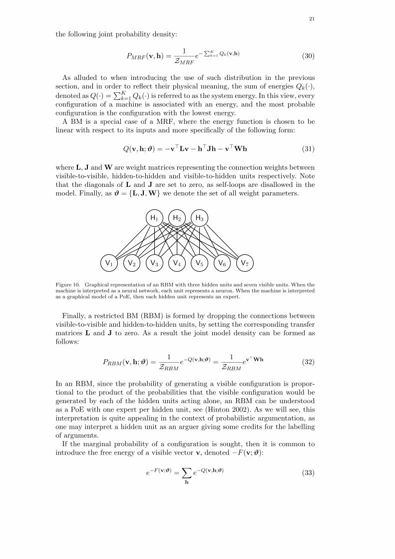
where L, J and W are weight matrices representing the connection weights betweenvisible-to-visible, hidden-to-hidden and visible-to-hidden units respectively. Notethat the diagonals of L and J are set to zero, as self-loops are disallowed in themodel. Finally, as ϑ = L,J,W we denote the set of all weight parameters.

H1 H2 H3

V1 V2 V3 V4 V5 V6 V7

Figure 10. Graphical representation of an RBM with three hidden units and seven visible units. When themachine is interpreted as a neural network, each unit represents a neuron. When the machine is interpretedas a graphical model of a PoE, then each hidden unit represents an expert.

Finally, a restricted BM (RBM) is formed by dropping the connections betweenvisible-to-visible and hidden-to-hidden units, by setting the corresponding transfermatrices L and J to zero. As a result the joint model density can be formed asfollows:

PRBM (v,h;ϑ) =1

ZRBMe−Q(v,h;ϑ) =

1

ZRBMev

>Wh (32)

In an RBM, since the probability of generating a visible configuration is propor-tional to the product of the probabilities that the visible configuration would begenerated by each of the hidden units acting alone, an RBM can be understoodas a PoE with one expert per hidden unit, see (Hinton 2002). As we will see, thisinterpretation is quite appealing in the context of probabilistic argumentation, asone may interpret a hidden unit as an arguer giving some credits for the labellingof arguments.

If the marginal probability of a configuration is sought, then it is common tointroduce the free energy of a visible vector v, denoted −F (v;ϑ):

e−F (v;ϑ) =∑h

e−Q(v,h;ϑ) (33)

22

so that

PRBM (v;ϑ) =e−F (v;ϑ)

ZRBM(34)

Notice that the free energy can be computed in a time linear in the number ofhidden units, see Hinton (2012).

When training a machine, the primary objective is to estimate the optimal modelweights ϑ∗ minimising the system’s energy Q(·) for a given set of N observationsdenoted as vnNn=1.

RBMs are usually trained by means of ‘Maximum Likelihood Estimation’ (MLE);although alternative approaches do exist in the literature, they usually introducea significant computational burden. By employing MLE we aim at estimating theoptimal model parameter configuration ϑ∗, which maximises the marginal log-likelihood for a given set ofN observations vnNn=1 which are assumed independentand identically distributed (i.i.d. - and thus the probability distribution of the Nobservations is the product of the probabilities for each observation):

lnPRBM

(vnNn=1 |ϑ

)= ln

N∏n=1

PRBM (vn|ϑ) =

N∑n=1

lnPRBM (vn|ϑ) (35)

From an alternative perspective, we aim at adjusting the model parameters so asto fit the true distribution of a training dataset. A measure of the discrepancybetween the true data distribution, denoted P (v), and the RBM density, denotedas PRBM (v|ϑ), is the Kullback-Leibler divergence (KL divergence), henceforth de-noted as DKL:

DKL =∑v

P (v) lnP (v)

PRBM (v)= EP (v) [lnP (v)]− EP (v) [lnPRBM (v|ϑ)] (36)

The first expectation is basically the entropy of P (v) and it is thus constantwith respect to the model parameters ϑ. Therefore the KL divergence is minimalwhen the second term is maximal. The second term is the expected log-likelihoodwhich can be approximated as an average of the finite number of N observationas follows: EP (v) [lnPRBM (v)] ≈ 1

N

∑Nn=1 lnPRBM (vn). In the asymptotic case,

where N → +∞, this approximation tends to the exact expected log-likelihood.Therefore, in order to minimize the KL divergence between the true and modeldistributions it is sufficient to maximise the log data likelihood. To do so, however,we first need to obtain the marginal log-likelihood PRBM (v|ϑ) of the RBM bysumming-out the hidden variables h as follows:

lnPRBM (v|ϑ) = ln∑h

PRBM (v,h|ϑ) (37)

= ln∑h

1

ZRBMe−Q(v,h) (38)

= ln∑h

e−Q(v,h) − ln∑h

∑v

e−Q(v,h) (39)

Note that the normalisation constant ZRBM =∑

h

∑v e−Q(v,h) is intractable

23

and thus the joint distribution is not directly accessible to us. Maximizing thelog-likelihood is usually achieved via gradient methods. Differentiate Equation 39yields:

∂ lnPRBM (v|ϑ)

∂ϑ= EPRBM (h|v)

[−∂Q(v,h)

∂ϑ

]− EPRBM (v,h)

[−∂Q(v,h)

∂ϑ

](40)

The first term is the expectation of the probabilities of hidden units given anobserved datapoint under the current model of the RBM, and thus it does not posea significant challenge. The second term is the expectation of the joint probabilityof visible and hidden units: as mentioned above, it is intractable as we are unableto directly normalise the joint distribution. For that reason, the gradient is mostfrequently approximated by means of ‘Contrastive Divergence’ (CD) (Hinton 2002),which has proven to be a fast and reasonably effective way to perform learning forRBMs.

CD is based on a simple principle, according to which it is sufficient to approx-imate the expectations in Equation 40, using only one value of v and h. Morespecifically we employ the following approximations:

EPRBM (h|v)

[− ∂

∂ϑQ(v,h)

]∼= −

∂

∂ϑQ(v0,h0) (41)

EPRBM (v,h)

[− ∂

∂ϑQ(v, h)

]∼= −

∂

∂ϑQ(vk,hk) (42)

where (v0,h0) and (vk,hk) are computed according to the following process:

(1) ”Clamp” v0 to an observed datapoint:

v0 = vn (43)

(2) Draw h0 from its conditional density:

h0 ∼ PRBM (h|v0) (44)

(3) Obtain (vk,hk) after k Gibbs samples t = 1, . . . , k as follows:

vt ∼ PRBM (v|ht−1) (45)

ht ∼ PRBM (h|vt) (46)

CD-k is applied by using the pair (vk,hk) as obtained by step 3 with k itera-tions. The conditional expectations necessary for the aforementioned draws, are asfollows:

PRBM (vi = 1|h) = σ (Q(vi = 1)) (47)

PRBM (hj = 1|v) = σ (Q(hj = 1)) (48)

where σ(x) = 1/(1 + e−x) is the sigmoid logistic function, and Q(vi = 1) andQ(hj = 1) are the energies of activation of a visible and hidden node, respectively,

24

that is, the sum of the weights of connections from other active nodes:

Q(vi = 1) = Wi:h (49)

Q(hj = 1) = vTW:j (50)

where Wi: and W:j we denote the ith row and jth column of the weight matrix Wrespectively. Concluding the weight parameter updates are given as follows:

∆wij = ε(v0i h

0j − vki hkj ) (51)

where ε scales the change. In practice many tricks exist to improve the training(see the guide by Hinton (2012) for details), including adaptive learning rates andadvanced gradient techniques such as Nesterov gradient, and the weights may beupdated after a so-called epoch, i.e. after estimating the gradient on ‘mini-batches’which are small sets of (typically 10 to 100) examples.

The use of the logistic function in Equation 47 can be generalized to the case ofa unit with K alternative states (such a unit is called a softmax unit), in this casethe probability to draw the unit in the state j is as follows:

Pj =eQj∑Ki=1 e

Qi

(52)

A softmax unit can be seen as a set of binary units constrained so that only one ofthe K configurations occurs. Training for softmax units is identical to the trainingfor standard binary units.

To generate samples from the learned model, Gibbs sampling is usually employed(Murphy 2012), by iteratively sampling all random variables from their conditionalprobability densities. We also refer to that process as a ”free run”. More specifically,we begin each free run from a random initial point (v0,h0) and progressively drawsamples t = 1, 2, 3, . . . as follows:

vti ∼ PRBM (vi|ht−1),∀i ∈ [1, D] (53)

htj ∼ PRBM (hj |vt), ∀j ∈ [1,K] (54)

The exact conditionals for the Gibbs sampler are given in Equation 47 and 48. Thebipartite structure of an RBM allows for the use of efficient block Gibbs sampling,where visible units are simultaneously sampled given fixed values of the hiddenunits, and hidden units are simultaneously sampled given the visible units.

As the samples for learning and the samples in the generative mode are similarlydrawn, BMs offer the possibility to learn a compact model of a distribution whiledrawing samples from the model. In this perspective, instead of reinitialising theMarkov chain to an observed data point after each weight update, we may initialisethe Markov Chain at the state in which it ended after k iterations, also referred aspersistent CD (Tieleman 2008).

Whatever the learning procedure, the number of hidden units used in an RBMhas a strong influence on its ability to learn distributions. Roux and Bengio (2008)showed that when the number of hidden nodes of an RBM is increased, thereare weight values for the new nodes that guarantee improvement in the KL diver-gence between the data distribution and the model distribution. In particular, theyshowed that any distribution over a set 0, 1D can be approximated arbitrarilywell (in the sense of the KL divergence) with an RBM with K + 1 hidden nodes

25

where K is the number of input vectors whose probability is not 0. In practice, thevalue of the number of hidden nodes is often chosen on the basis of experience (seeHinton (2012) for a recipe) and the desired approximation.

7. Argumentative Boltzmann Machines

To construct a BM that embodies probabilistic abstract argumentation, we refor-mulate argumentative labelling as a Gibbs sampling within the binary setting ofBMs. Yet different machines can be built to perform the labelling of argumentationgraphs in such setting. For this reason, we are in fact in front of different typesof machines called argumentative BMs in the sense that different machines can beproposed to label arguments. We are proposing two types here and we will focuson the second.

A first type of argumentative machine consists in a machine where the on, off-labelling of an argument is represented by a visible node. We call this machine aon, off-labelling machine. In this machine, an argument is on (thus labelled ei-ther in or out or un with respect to the grounded semantics) if, and only if, thecorresponding node is switched on, and an argument is off if, and only if, the corre-sponding node is switched off. When learning, any example clamped to the machineis a on, off-labelling (i.e. a sub-graph) to indicate whether an argument is on oroff. So, a on, off-labelling machine shall learn a distribution of on, off-labellingsand, when running in free mode, it shall sample on, off-labellings according to thelearned distribution. Once a legal on, off-labelling is produced, one can computethe entailed grounded in, out, un, off-labelling using Algorithm 1. The advantageof such a machine is its simplicity: it boils down to a conventional BM chainedwith an algorithm to compute the grounded in, out, un, off-labelling of sampledgraphs (or any other labelling based on the provision of such algorithm to computethis labelling). A major disadvantage is that this machine cannot discriminate in,out or un labellings (limiting the discriminative mode and possibly hindering pos-sible useful mining of the network in search of relations amongst the statuses ofarguments), and one cannot possibly guess the in, out, un, off-labelling of somearguments given the in, out, un, off-labelling of some other arguments.

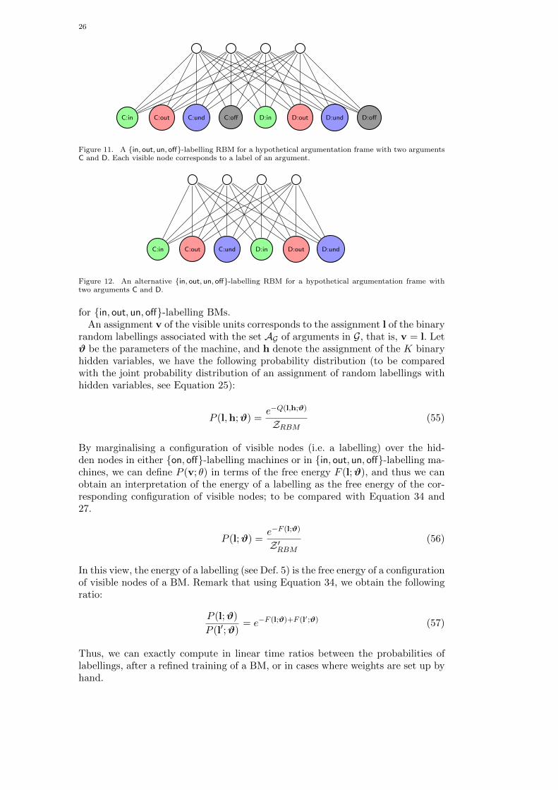
To address the limitations of on, off-labelling BMs, we propose an alterna-tive type of argumentative machines where a configuration of visible nodes rep-resents a in, out, un, off-labelling. Such machines are henceforth referred to as ain, out, un, off-labelling machines. Different sorts of in, out, un, off-labelling ma-chines are possible. The most instinctive way to construct such a machine is bypairing any label of every argument with one visible node, and only one. Whena visible node has value 1 then the argument shall be labelled accordingly, if thenode has value 0 then there is no such labelling. An example of a in, out, un, off-labelling RBM is given in Figure 11.

An alternative in, out, un, off-labelling machine is a machine where each of thelabels in, out and un is paired with one visible node, and only one. Then an argumentis labelled off when all the visible nodes of this argument are switched off (i.e. takethe value 0). An example of this sort of in, out, un, off-labelling BM is given inFigure 12. The obvious advantage here is the reduction of the space complexity,and a priori the training time (since there are fewer weights to train).

As for notation, the energy of activation of an argument A being labelled inwill be denoted Q(in(A)), and similarly Q(out(A)) will denote the energy of Alabelled out, Q(un(A)) for A labelled un, and Q(off(A)) for A labelled off. Sincethe four statuses of an argument is encoded by four different configurations of theassociated units, we have the possibility to consider softmax units (see Section 6)

26

C:in C:out C:und C:off D:in D:out D:und D:off

Figure 11. A in, out, un, off-labelling RBM for a hypothetical argumentation frame with two argumentsC and D. Each visible node corresponds to a label of an argument.

C:in C:out C:und D:in D:out D:und

Figure 12. An alternative in, out, un, off-labelling RBM for a hypothetical argumentation frame withtwo arguments C and D.

for in, out, un, off-labelling BMs.An assignment v of the visible units corresponds to the assignment l of the binary

random labellings associated with the set AG of arguments in G, that is, v = l. Letϑ be the parameters of the machine, and h denote the assignment of the K binaryhidden variables, we have the following probability distribution (to be comparedwith the joint probability distribution of an assignment of random labellings withhidden variables, see Equation 25):

P (l,h;ϑ) =e−Q(l,h;ϑ)

ZRBM(55)

By marginalising a configuration of visible nodes (i.e. a labelling) over the hid-den nodes in either on, off-labelling machines or in in, out, un, off-labelling ma-chines, we can define P (v; θ) in terms of the free energy F (l;ϑ), and thus we canobtain an interpretation of the energy of a labelling as the free energy of the cor-responding configuration of visible nodes; to be compared with Equation 34 and27.

P (l;ϑ) =e−F (l;ϑ)

Z ′RBM(56)

In this view, the energy of a labelling (see Def. 5) is the free energy of a configurationof visible nodes of a BM. Remark that using Equation 34, we obtain the followingratio:

P (l;ϑ)

P (l′;ϑ)= e−F (l;ϑ)+F (l′;ϑ) (57)

Thus, we can exactly compute in linear time ratios between the probabilities oflabellings, after a refined training of a BM, or in cases where weights are set up byhand.

27

Focusing on grounded in, out, un, off-labelling machines, once a machine is welltrained, the free energy of any illegal labelling shall be very high compared to legallabellings, in a manner such that the probability of any illegal labelling will be closeto 0. So, a standard Gibbs sampling may sample illegal labellings with probabilityclose to 0.

To ensure the production of grounded in, out, un, off-labellings, we may checkex post whether a produced labelling is grounded and discard it if not, but thissolution may involve extra computation that may slow down the production ofgrounded labellings. So we propose to tune the Algorithm 1 for computing thegrounded in, out, un-labelling of an argumentation graph into a probabilisticvariant as given in the Algorithm 2. This Algorithm 2 is called a ‘labelling randomwalk ’ or more specifically a grounded in, out, un, off-labelling random walk inorder to emphasise that first of all it features a random walk, on which any Gibbssampling of a BM is based, and second that it is constrained by the constructionof a grounded in, out, un, off-labelling. This walk shall be used to sample visibleunits so that we ensure that grounded in, out, un, off-labellings are sampled, andsuch a sampling is called a grounded in, out, un, off-sampling.

For the sake of the clarity of the presentation, we adopt the following notation.An argument A is labelled in with respect to a labelling li if, and only if,

• A is not labelled in li, and

• ∀B : if B attacks A then B ∈ out(li) ∪ off(li), and

• A is drawn in: u ≤ eQ(in(A))/Z(A) where u is a random number in [0, 1] drawnfrom an uniform distribution, and

Z(A) = eQ(in(A)) + eQ(out(A)) + eQ(un(A)) + eQ(off(A))

We denote IN(li) the set of arguments eventually labelled in with respect to alabelling li. An argument A fulfilling the first two conditions but not drawn in issaid ‘inable’, abbreviated inable(li, A).

An argument A is labelled out with respect of the labellings li and li+1 if, and onlyif,

• A is not labelled in li, and

• ∃B : B attacks A and B ∈ in(li+1), and

• A is drawn out: u ≤ eQ(out(A))/Z(A).

We denote OUT(li, li+1) the set of arguments eventually labelled out with respectto the labellings li and li+1. An argument A fulfilling the first two conditions butnot drawn out is said ‘outable’, abbreviated outable(li, li+1, A).

An argument A is labelled off with respect to labellings li and li+1 if

• A is not labelled in li, and

• A was not labelled in or out, i.e. inable(li, A) or outable(li, li+1, A).

We denote OFF1(li, li+1) the set of arguments labelled off this way.

Finally, an argument A is labelled off with respect to a labelling li+1 if

• A is not labelled in li+1, and

• A is drawn off: u ≤ eQ(off(A))/Z(A).

We denote OFF2(li+1) the set of arguments labelled off this way.

28

With this notation, we can now present a simple version of the groundedin, out, un, off-labelling random walk as given in Algorithm 2.

Algorithm 2 Grounded in, out, un, off-labelling random walk.

1: input Machine parameters ϑ, argumentation frame G2: l0 = (∅, ∅, ∅, ∅)3: repeat4: l′0 ← li5: repeat6: in(l′i+1)← in(l′i) ∪ IN(l′i)

7: out(l′i+1)← out(l′i) ∪ OUT(l′i, l′i+1)

8: off(l′i+1)← off(l′i) ∪ OFF1(l′i, l′i+1)

9: until l′i = l′i+110: li+1 ← l′i11: off(li+1)← off(li) ∪ OFF2(li+1)12: until li = li+1

13: return (in(li), out(li), A− in(li) ∪ out(li) ∪ off(li), off(li))

The labelling random walk consists of an outer loop and an inner loop. The innerloop draws the labelling in and out of arguments with respect to their probability.The inner loop begins by labelling in all arguments not being attacked or whoseattackers are out (line 6), and then it iteratively labels out any argument attackedby an argument labelled in (line 7). If an argument eligible for a label in or out isnot labelled as such, then it is labelled off (line 8). The iteration of the inner loopcontinues until no more arguments can be labelled in or out (line 9). Any argumentremaining unlabelled is then labelled off with its respective probability (line 11).If there is an argument labelled off, then the labelling proceeds in the inner loop.If there is no argument labelled off, then the walk terminates by finally labellingun all remaining arguments (line 13).

When learning, the machine will be shown a set of training examples where anexample is a set of labelled arguments. To clamp the visible nodes of a machine witha set of labelled arguments, a visible node will be set at 1 if its labelling matches theexample, otherwise it is set at 0. If a training example does not match any groundedin, out, un, off-labelling of the hypothetical framework then it suggests that thehypothetical framework shall be changed and be adapted, but noisy settings mayalso occur. These issues are not addressed here. Notice that the learning procedureand the labelling walk are kept separated, thus we shall use the walk with anystate-of-the-art learning algorithms or future improvements.

When labelling arguments with the labelling random walk, if the weight matrixL is not set to 0 (e.g. in the case of a general BM) then the order in which the argu-ments are labelled matters. If the matrix L is set to 0, as in the case of an RBM, thenthe order of labelling does not matter. Thus a grounded in, out, un, off-labellingmachine based on a conventional general BM exhibits a discrepancy between anideal purely random walk amongst possible states of the machine (as suggestedby a general BM setting) and the proposed labelling walk (Algorithm 2) meant toensure grounded in, out, un, off-labelling. Indeed, this labelling walk is not purelyrandom, as visible nodes are now considered in an order regimented by the con-struction of a grounded in, out, un, off-labelling. Thus, in order to integrate theargumentative constraints during all the walk, the RBM model appears more ap-propriate as the sampling of the visible nodes will be performed using the labelling

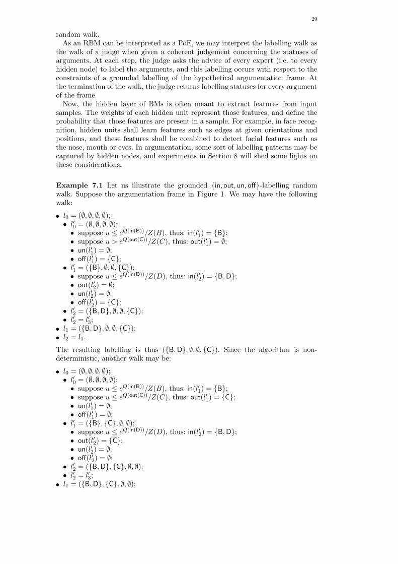
29

random walk.As an RBM can be interpreted as a PoE, we may interpret the labelling walk as

the walk of a judge when given a coherent judgement concerning the statuses ofarguments. At each step, the judge asks the advice of every expert (i.e. to everyhidden node) to label the arguments, and this labelling occurs with respect to theconstraints of a grounded labelling of the hypothetical argumentation frame. Atthe termination of the walk, the judge returns labelling statuses for every argumentof the frame.

Now, the hidden layer of BMs is often meant to extract features from inputsamples. The weights of each hidden unit represent those features, and define theprobability that those features are present in a sample. For example, in face recog-nition, hidden units shall learn features such as edges at given orientations andpositions, and these features shall be combined to detect facial features such asthe nose, mouth or eyes. In argumentation, some sort of labelling patterns may becaptured by hidden nodes, and experiments in Section 8 will shed some lights onthese considerations.

Example 7.1 Let us illustrate the grounded in, out, un, off-labelling randomwalk. Suppose the argumentation frame in Figure 1. We may have the followingwalk:

• l0 = (∅, ∅, ∅, ∅);• l′0 = (∅, ∅, ∅, ∅);• suppose u ≤ eQ(in(B))/Z(B), thus: in(l′1) = B;• suppose u > eQ(out(C))/Z(C), thus: out(l′1) = ∅;• un(l′1) = ∅;• off(l′1) = C;

• l′1 = (B, ∅, ∅, C);• suppose u ≤ eQ(in(D))/Z(D), thus: in(l′2) = B,D;• out(l′2) = ∅;• un(l′2) = ∅;• off(l′2) = C;

• l′2 = (B,D, ∅, ∅, C);• l′2 = l′3;

• l1 = (B,D, ∅, ∅, C);• l2 = l1.

The resulting labelling is thus (B,D, ∅, ∅, C). Since the algorithm is non-deterministic, another walk may be:

• l0 = (∅, ∅, ∅, ∅);• l′0 = (∅, ∅, ∅, ∅);• suppose u ≤ eQ(in(B))/Z(B), thus: in(l′1) = B;• suppose u ≤ eQ(out(C))/Z(C), thus: out(l′1) = C;• un(l′1) = ∅;• off(l′1) = ∅;

• l′1 = (B, C, ∅, ∅);• suppose u ≤ eQ(in(D))/Z(D), thus: in(l′2) = B,D;• out(l′2) = C;• un(l′2) = ∅;• off(l′2) = ∅;

• l′2 = (B,D, C, ∅, ∅);• l′2 = l′3;

• l1 = (B,D, C, ∅, ∅);

30

• l2 = l1.

So in this last walk, the labelling (B,D, C, ∅, ∅) was returned. In another run,when computing l′0 in the first time we may obtain l′1 = (∅, ∅, ∅, B), and thealgorithm may return (∅, ∅, C,D, B).

For any possible input, the grounded in, out, un, off-labelling random walk (al-gorithm 2) terminates, i.e. it exits by returning a labelling of all arguments ofthe argumentation frame. Indeed at each iteration of the outer loop, at least oneargument is labelled until termination when all arguments get labelled.

Theorem 7.2 : (Termination) The grounded in, out, un, off-labelling randomwalk terminates.

Proof : To prove the termination, we consider the sequence of pairs(A0, l0), (A1, l1), . . . , (An, ln) where Ai and li are the set of unlabelled argumentsand the set of labelled arguments i.e. a partial labelling (respectively) at the be-ginning of the iteration i of the outer loop. At each iteration i, the cardinality ofAi is strictly inferior to the cardinality of Ai−1. At some point, there is no furtherargument to label, then ln = ln−1 and thus the algorithm terminates.

We say that a labelling algorithm is sound with respect to a type of labelling if, andonly if, it returns a labelling of the argumentation frame as defined with respect tothis type of labelling. When the grounded in, out, un, off-labelling random walkterminates, it necessarily returns a grounded in, out, un, off-labelling of the argu-mentation frame, it is thus sound with respect to the grounded in, out, un, off-labelling.

Theorem 7.3 : (Soundness) The grounded in, out, un, off-labelling random walkis sound.

Proof : To prove the soundness, we consider any terminated sequence(A0, l0), (A1, l1), . . . , (An, ln), and we show that ln is a grounded in, out, un, off-labelling. To show that ln is a grounded in, out, un, off-labelling, we consider thelabelled argumentation sub-graph H induced by the arguments labelled on and weshow that this graph has a grounded in, out, un-labelling. To see that the graphH has a grounded in, out, un-labelling l′, it is sufficient to observe that l′ is a com-plete labelling, and in(l′) is minimal (because no less arguments can be labelled in).Therefore, ln is a grounded in, out, un, off-labelling.

Moreover, we say that a labelling algorithm is complete with respect to a type oflabelling if, and only if, it can return any labelling of the argumentation frameas defined with respect to this type of labelling. The grounded in, out, un, off-labelling random walk can return any grounded in, out, un, off-labelling of theargumentation frame, it is thus complete.

Theorem 7.4 : (Completeness) The grounded in, out, un, off-labelling randomwalk is complete.

Proof : To prove the completeness, we demonstrate that for anygrounded in, out, un, off-labelling l, there exists a terminated sequence(A0, l0), (A1, l1), . . . , (An, ln) where ln = l. For any terminal groundedin, out, un, off-labelling L, there exists a unique graph induced by the ar-guments labelled present in L, and thus we have to show that the walk can returnthis graph. However, the walk can return any set of arguments labelled off, andthus any induced sub-graph. Consequently, for any grounded in, out, un, off-labelling l, there exists a terminated sequence (A0, l0), (A1, l1), . . . , (An, ln) withln = l.

31

As mentioned earlier, once a machine is trained, the free energy of any illegallabelling shall be very high compared to legal labellings, in a manner such that theprobability of any illegal labelling will be close to 0. So, a standard Gibbs sam-pling may sample illegal labellings with probability close to 0. Since the groundedin, out, un, off-labelling random walk is sound, we ensure that illegal labellingswill not be sampled. And since the random walk is sound and complete, thena well trained grounded in, out, un, off-labelling machine coupled with a sampleprocedure like the random labelling walk shall produce a sound estimation of theprobability distributions. Experiments in the next section will bring some evidencesin this regard, within the boundaries of the experimented training procedures.

Concerning time complexity, the walk is a slight adaptation of the Algorithm 1for a probabilistic setting, meant to keep its polynomial complexity.

Theorem 7.5 : (Time complexity) Time complexity of the groundedin, out, un, off-labelling random walk is polynomial.

Proof : At each iteration of the inner loop, one argument at least is labelled, oth-erwise the algorithm terminates. Therefore, when the input argumentation framehas N arguments, then there are N iterations at worse. For each iteration, the sta-tuses of N argument has to be checked with respect to the statuses of N argumentsin the worst case. The time complexity of this inner loop is thus polynomial. Whenthe inner loop terminates, one iteration of the outer loop completes by checking thestatuses of remaining unlabelled arguments, and the outer loop iterates N timesat worse. Therefore, the time complexity of the grounded in, out, un, off-labellingrandom walk is polynomial.

Concerning space complexity, a major benefit of the proposed approach is totackle the exponential space complexity of the sample space of a probabilisticargumentation frame (see Definition 4.1) by a compact machine whose the spacecomplexity is reduced to weight matrices.

Theorem 7.6 : (Space complexity) Space complexity of the groundedin, out, un, off-labelling random walk is O(max(|v| × |v|, |h| × |h|, |v| × |h|)).

Proof : A BM can be described by two binary random vectors corresponding tonodes vectors v and h, and matrices L, J and W (corresponding to the strengthof the edges between hidden and visible nodes, see Figure 11), an hypotheticalargumentation graph and machine parameters. The two binary vectors, the hypo-thetical argumentation graph and machine parameters require minimal space, thusthe memory requirements are dominated by the real-valued edge matrices L, J andW . We need a weight to describe each pairwise interaction amongst hidden andvisible nodes, thus it holds that the dimensions of the matrices are |v| × |v| for L,|h| × |h| for J, and |v| × |h| for W.

In case of an RBM, we have L = 0 and J = 0, therefore the space complexity isreduced to O(|v| · |h|) in this case.

The labelling random walk is designed to ensure the production of groundedin, out, un, off-labellings. By sampling grounded in, out, un, off-labellings, wecan then evaluate the probability of a labelling or the marginal probability ofthe labelling of some subset of arguments. The walk allows us to sample groundedin, out, un, off-labellings on demand (instead of checking ex post whether a sam-pled labelling is a grounded in, out, un, off-labelling and waiting that such a la-belling eventually pops up), saving thus computational time when a valid labellingis requested. However, as BMs learn by mistakes too and since the random la-belling walk may stuck the underlying Markov chain of the Gibbs sampling into

32

some minima (corresponding to grounded in, out, un, off-labellings), one may seeka balance between the use of the random labelling walk and an ordinary samplingof visible units as given in Equation 53. This point will be experimentally exploredby using an argumentative mixing rate in the next section.

8. Experiments

The experiments regard the use and effects of the grounded in, out, un, off-labelling random walk (Algorithm 2) in the learning mode and generative mode ofan RBM.

To get experimental insights into the use of the grounded in, out, un, off-labelling random walk, we alternated grounded in, out, un, off-samplings and or-dinary Gibbs samplings of conventional machines with an argumentative mixingrate pm ∈ [0, 1]: we draw a random number u between [0, 1] from a uniform distribu-tion, and if u ≤ pm then an ordinary sampling is used to sample a configuration ofvisible nodes, otherwise a grounded in, out, un, off-sampling is performed. Hence,if the rate pm = 0 then only grounded in, out, un, off-samplings are performed.If the rate pm = 1, then we have a conventional RBM. This rate should not beconfused with the mixing rate of the Markov chain, i.e. the rate of convergence tothe Markov chain equilibrium distribution.

The statistical distance between the empirical distribution P of the labellingsdrawn from a training dataset (approximating the source distribution) and thedistribution P ′ learned by a machine was measured using the KL divergence (seeEquation 36) and the total variation distance (TV distance) denoted δ(P, P ′) anddefined as follows:

δ(P, P ′) =1

2

∑l∈S|P (l)− P ′(l)| (58)

where S are the examples drawn from the training dataset.The experiments concerned (i) a tiny hypothetical argumentation frame so that

the source distribution, the distribution of reconstructed labellings (at the endof a training phase) and the distribution of generated labellings (at the end ofa generative phase) could be extensively compared and that the weights couldbe examined (ii) a small hypothetical argumentation frame to test RBMs withdifferent argumentative mixing rates and entropies of the training distributions(iii) larger frames to reconnoiter the limits of the tested machines. In all cases, thedatasets were artificially generated (without any noise), so that this evaluation wasnot dependent of any particular domain. To build these datasets, each groundedin, out, un, off-labelling was associated a random energy and examples amongstlabellings were drawn from the associated Gibbs–Boltzmann distribution.

8.1. First experiment

The first experiment regards the training of a grounded in, out, un, off-labellingmachine based on a tiny hypothetical argumentation frame of 5 arguments, see Fig-ure 13 - inducing 45 = 1024 different possible in, out, un, off-labellings, amongstwhich 32 grounded labellings.

The training consisted of 1000 passes over small batches, each containing 100grounded in, out, un, off-labellings. The weights were updated after each pass, us-ing adaptive learning rate (in the interval [0, 1]) and Nestorov accelerated gradient.

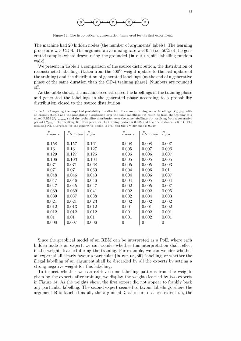
33

B C D E F

Figure 13. The hypothetical argumentation frame used for the first experiment.

The machine had 20 hidden nodes (the number of arguments’ labels). The learningprocedure was CD-4. The argumentative mixing rate was 0.5 (i.e. 50% of the gen-erated samples where drawn using the grounded in, out, un, off-labelling randomwalk).

We present in Table 1 a comparison of the source distribution, the distribution ofreconstructed labellings (taken from the 500th weight update to the last update ofthe training) and the distribution of generated labellings (at the end of a generativephase of the same duration than the CD-4 training phase). Numbers are roundedoff.

As the table shows, the machine reconstructed the labellings in the training phaseand generated the labellings in the generated phase according to a probabilitydistribution closed to the source distribution.

Table 1. Comparing the empirical probability distribution of a source training set of labellings (Psource with

an entropy 2.681) and the probability distribution over the same labellings but resulting from the training of a

mixed RBM (Ptraining) and the probability distribution over the same labellings but resulting from a generative

period (Pgen). The resulting KL divergence for the training period is 0.005 and the TV distance is 0.017. The

resulting KL divergence for the generative period is 0.01 and the TV distance is 0.029.

Psource Ptraining Pgen

0.158 0.157 0.1610.13 0.13 0.1270.129 0.127 0.1250.106 0.103 0.1040.071 0.071 0.0680.071 0.07 0.0690.048 0.046 0.0430.047 0.046 0.0460.047 0.045 0.0470.039 0.039 0.0410.039 0.037 0.0380.021 0.021 0.0230.012 0.013 0.0120.012 0.012 0.0120.01 0.01 0.010.008 0.007 0.006

Psource Ptraining Pgen

0.008 0.008 0.0070.005 0.007 0.0060.005 0.006 0.0070.005 0.005 0.0050.005 0.005 0.0030.004 0.006 0.010.004 0.006 0.0070.004 0.005 0.0040.002 0.005 0.0070.002 0.002 0.0050.002 0.004 0.0030.002 0.002 0.0020.001 0.001 0.0020.001 0.002 0.0010.001 0.002 0.0010 0 0

Since the graphical model of an RBM can be interpreted as a PoE, where eachhidden node is an expert, we can wonder whether this interpretation shall reflectin the weights learned during the training. For example, we can wonder whetheran expert shall clearly favour a particular in, out, un, off labelling, or whether theillegal labelling of an argument shall be discarded by all the experts by setting astrong negative weight for this labelling.

To inspect whether we can retrieve some labelling patterns from the weightsgiven by the experts after training, we display the weights learned by two expertsin Figure 14. As the weights show, the first expert did not appear to frankly backany particular labelling. The second expert seemed to favour labellings where theargument B is labelled as off, the argument C as in or to a less extent un, the

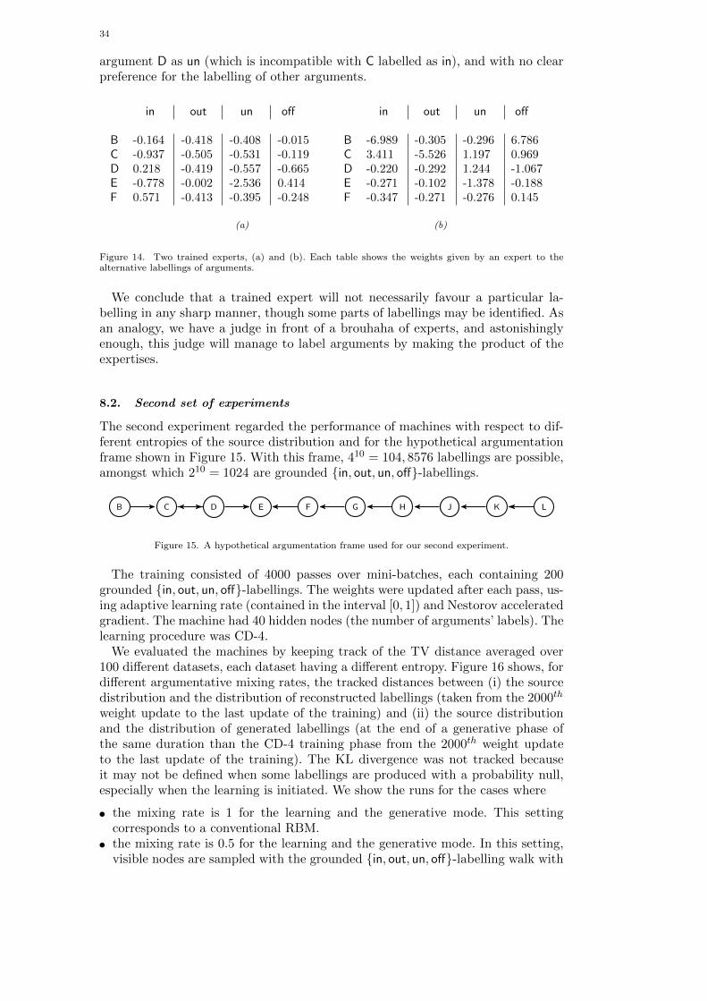
34

argument D as un (which is incompatible with C labelled as in), and with no clearpreference for the labelling of other arguments.

in out un off

B -0.164 -0.418 -0.408 -0.015C -0.937 -0.505 -0.531 -0.119D 0.218 -0.419 -0.557 -0.665E -0.778 -0.002 -2.536 0.414F 0.571 -0.413 -0.395 -0.248

(a)

in out un off

B -6.989 -0.305 -0.296 6.786C 3.411 -5.526 1.197 0.969D -0.220 -0.292 1.244 -1.067E -0.271 -0.102 -1.378 -0.188F -0.347 -0.271 -0.276 0.145

(b)

Figure 14. Two trained experts, (a) and (b). Each table shows the weights given by an expert to thealternative labellings of arguments.

We conclude that a trained expert will not necessarily favour a particular la-belling in any sharp manner, though some parts of labellings may be identified. Asan analogy, we have a judge in front of a brouhaha of experts, and astonishinglyenough, this judge will manage to label arguments by making the product of theexpertises.

8.2. Second set of experiments

The second experiment regarded the performance of machines with respect to dif-ferent entropies of the source distribution and for the hypothetical argumentationframe shown in Figure 15. With this frame, 410 = 104, 8576 labellings are possible,amongst which 210 = 1024 are grounded in, out, un, off-labellings.

B C D E F G H IJ K L

Figure 15. A hypothetical argumentation frame used for our second experiment.

The training consisted of 4000 passes over mini-batches, each containing 200grounded in, out, un, off-labellings. The weights were updated after each pass, us-ing adaptive learning rate (contained in the interval [0, 1]) and Nestorov acceleratedgradient. The machine had 40 hidden nodes (the number of arguments’ labels). Thelearning procedure was CD-4.

We evaluated the machines by keeping track of the TV distance averaged over100 different datasets, each dataset having a different entropy. Figure 16 shows, fordifferent argumentative mixing rates, the tracked distances between (i) the sourcedistribution and the distribution of reconstructed labellings (taken from the 2000th

weight update to the last update of the training) and (ii) the source distributionand the distribution of generated labellings (at the end of a generative phase ofthe same duration than the CD-4 training phase from the 2000th weight updateto the last update of the training). The KL divergence was not tracked becauseit may not be defined when some labellings are produced with a probability null,especially when the learning is initiated. We show the runs for the cases where

• the mixing rate is 1 for the learning and the generative mode. This settingcorresponds to a conventional RBM.

• the mixing rate is 0.5 for the learning and the generative mode. In this setting,visible nodes are sampled with the grounded in, out, un, off-labelling walk with

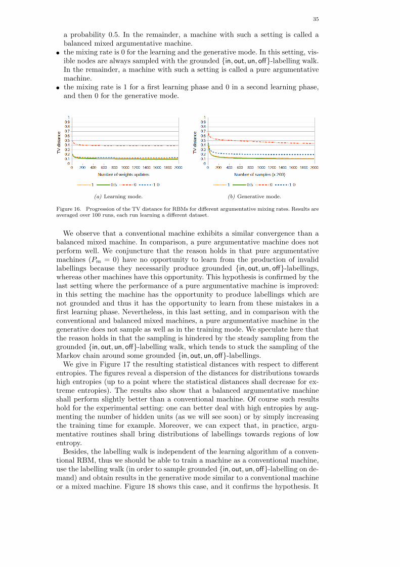
35

a probability 0.5. In the remainder, a machine with such a setting is called abalanced mixed argumentative machine.

• the mixing rate is 0 for the learning and the generative mode. In this setting, vis-ible nodes are always sampled with the grounded in, out, un, off-labelling walk.In the remainder, a machine with such a setting is called a pure argumentativemachine.

• the mixing rate is 1 for a first learning phase and 0 in a second learning phase,and then 0 for the generative mode.

(a) Learning mode. (b) Generative mode.

Figure 16. Progression of the TV distance for RBMs for different argumentative mixing rates. Results areaveraged over 100 runs, each run learning a different dataset.

We observe that a conventional machine exhibits a similar convergence than abalanced mixed machine. In comparison, a pure argumentative machine does notperform well. We conjuncture that the reason holds in that pure argumentativemachines (Pm = 0) have no opportunity to learn from the production of invalidlabellings because they necessarily produce grounded in, out, un, off-labellings,whereas other machines have this opportunity. This hypothesis is confirmed by thelast setting where the performance of a pure argumentative machine is improved:in this setting the machine has the opportunity to produce labellings which arenot grounded and thus it has the opportunity to learn from these mistakes in afirst learning phase. Nevertheless, in this last setting, and in comparison with theconventional and balanced mixed machines, a pure argumentative machine in thegenerative does not sample as well as in the training mode. We speculate here thatthe reason holds in that the sampling is hindered by the steady sampling from thegrounded in, out, un, off-labelling walk, which tends to stuck the sampling of theMarkov chain around some grounded in, out, un, off-labellings.

We give in Figure 17 the resulting statistical distances with respect to differententropies. The figures reveal a dispersion of the distances for distributions towardshigh entropies (up to a point where the statistical distances shall decrease for ex-treme entropies). The results also show that a balanced argumentative machineshall perform slightly better than a conventional machine. Of course such resultshold for the experimental setting: one can better deal with high entropies by aug-menting the number of hidden units (as we will see soon) or by simply increasingthe training time for example. Moreover, we can expect that, in practice, argu-mentative routines shall bring distributions of labellings towards regions of lowentropy.

Besides, the labelling walk is independent of the learning algorithm of a conven-tional RBM, thus we should be able to train a machine as a conventional machine,use the labelling walk (in order to sample grounded in, out, un, off-labelling on de-mand) and obtain results in the generative mode similar to a conventional machineor a mixed machine. Figure 18 shows this case, and it confirms the hypothesis. It

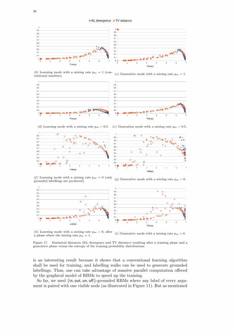
36

(b) Learning mode with a mixing rate pm = 1 (con-ventional machine).

(c) Generative mode with a mixing rate pm = 1.

(d) Learning mode with a mixing rate pm = 0.5. (e) Generation mode with a mixing rate pm = 0.5.

(f) Learning mode with a mixing rate pm = 0 (onlygrounded labellings are produced).

(g) Generative mode with a mixing rate pm = 0.

(h) Learning mode with a mixing rate pm = 0, aftera phase where the mixing rate pm = 1.

(i) Generative mode with a mixing rate pm = 0.

Figure 17. Statistical distances (KL divergence and TV distance) resulting after a training phase and agenerative phase versus the entropy of the training probability distributions.

is an interesting result because it shows that a conventional learning algorithmshall be used for training, and labelling walks can be used to generate groundedlabellings. Thus, one can take advantage of massive parallel computation offeredby the graphical model of RBMs to speed up the training.

So far, we used in, out, un, off-grounded RBMs where any label of every argu-ment is paired with one visible node (as illustrated in Figure 11). But as mentioned

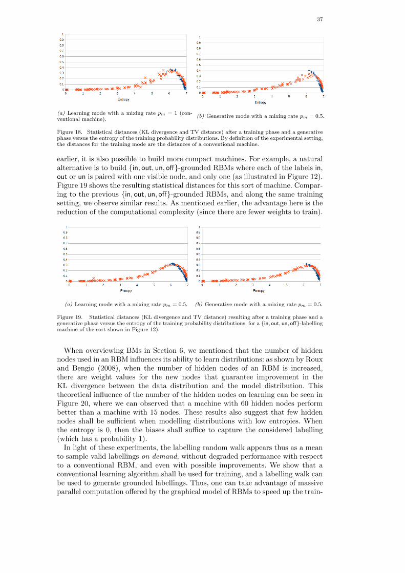
37

(a) Learning mode with a mixing rate pm = 1 (con-ventional machine).

(b) Generative mode with a mixing rate pm = 0.5.

Figure 18. Statistical distances (KL divergence and TV distance) after a training phase and a generativephase versus the entropy of the training probability distributions. By definition of the experimental setting,the distances for the training mode are the distances of a conventional machine.

earlier, it is also possible to build more compact machines. For example, a naturalalternative is to build in, out, un, off-grounded RBMs where each of the labels in,out or un is paired with one visible node, and only one (as illustrated in Figure 12).Figure 19 shows the resulting statistical distances for this sort of machine. Compar-ing to the previous in, out, un, off-grounded RBMs, and along the same trainingsetting, we observe similar results. As mentioned earlier, the advantage here is thereduction of the computational complexity (since there are fewer weights to train).

(a) Learning mode with a mixing rate pm = 0.5. (b) Generative mode with a mixing rate pm = 0.5.

Figure 19. Statistical distances (KL divergence and TV distance) resulting after a training phase and agenerative phase versus the entropy of the training probability distributions, for a in, out, un, off-labellingmachine of the sort shown in Figure 12).

When overviewing BMs in Section 6, we mentioned that the number of hiddennodes used in an RBM influences its ability to learn distributions: as shown by Rouxand Bengio (2008), when the number of hidden nodes of an RBM is increased,there are weight values for the new nodes that guarantee improvement in theKL divergence between the data distribution and the model distribution. Thistheoretical influence of the number of the hidden nodes on learning can be seen inFigure 20, where we can observed that a machine with 60 hidden nodes performbetter than a machine with 15 nodes. These results also suggest that few hiddennodes shall be sufficient when modelling distributions with low entropies. Whenthe entropy is 0, then the biases shall suffice to capture the considered labelling(which has a probability 1).

In light of these experiments, the labelling random walk appears thus as a meanto sample valid labellings on demand, without degraded performance with respectto a conventional RBM, and even with possible improvements. We show that aconventional learning algorithm shall be used for training, and a labelling walk canbe used to generate grounded labellings. Thus, one can take advantage of massiveparallel computation offered by the graphical model of RBMs to speed up the train-

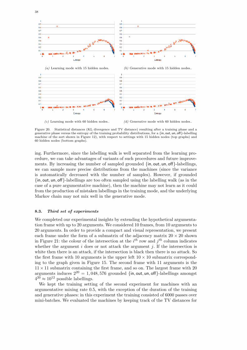
38

(a) Learning mode with 15 hidden nodes. (b) Generative mode with 15 hidden nodes..

(c) Learning mode with 60 hidden nodes.. (d) Generative mode with 60 hidden nodes..

Figure 20. Statistical distances (KL divergence and TV distance) resulting after a training phase and agenerative phase versus the entropy of the training probability distributions, for a in, out, un, off-labellingmachine of the sort shown in Figure 12), with respect to settings with 15 hidden nodes (top graphs) and60 hidden nodes (bottom graphs).

ing. Furthermore, since the labelling walk is well separated from the learning pro-cedure, we can take advantages of variants of such procedures and future improve-ments. By increasing the number of sampled grounded in, out, un, off-labellings,we can sample more precise distributions from the machines (since the varianceis automatically decreased with the number of samples). However, if groundedin, out, un, off-labellings are too often sampled using the labelling walk (as in thecase of a pure argumentative machine), then the machine may not learn as it couldfrom the production of mistaken labellings in the training mode, and the underlyingMarkov chain may not mix well in the generative mode.

8.3. Third set of experiments

We completed our experimental insights by extending the hypothetical argumenta-tion frame with up to 20 arguments. We considered 10 frames, from 10 arguments to20 arguments. In order to provide a compact and visual representation, we presenteach frame under the form of a submatrix of the adjacency matrix 20× 20 shownin Figure 21: the colour of the intersection at the ith row and jth column indicateswhether the argument i does or not attack the argument j. If the intersection iswhite then there is an attack, if the intersection is black then there is no attack. Sothe first frame with 10 arguments is the upper left 10× 10 submatrix correspond-ing to the graph given in Figure 15. The second frame with 11 arguments is the11× 11 submatrix containing the first frame, and so on. The largest frame with 20arguments induces 220 = 1, 048, 576 grounded in, out, un, off-labellings amongst420 ≈ 1012 possible labellings.

We kept the training setting of the second experiment for machines with anargumentative mixing rate 0.5, with the exception of the duration of the trainingand generative phases: in this experiment the training consisted of 6000 passes overmini-batches. We evaluated the machines by keeping track of the TV distances for

39

Figure 21. Adjacency matrix encoding argumentation graphs.

four runs for the different frames and for two entropies of datasets, 3.466 and 5.198.

(a) Learning mode. (b) Generative mode.

(c) Learning mode. (d) Generative mode.

Figure 22. TV distances resulting after a learning phase and a generative phase (with a mixing ratepm = 0.5) versus the number of arguments. For any argumentation graph, the entropy was fixed to 3.466(top) and 5.198 (bottom).

The resulting TV distances are given in Figure 22, for the two entropies 3.466and 5.198, between (i) the source distribution and the distribution of reconstructedlabellings (taken from the 2000th weight update to the last update of the training)and (ii) the source distribution and the distribution of generated labellings (at theend of a generative phase of the same duration than the CD-4 training phase fromthe 2000th weight update to the last update of the training).

We observe that learning degrades when the number of arguments augments andwhen the entropy increases. Results shall improve with a longer training, or byconsidering more advanced learning settings such as persistent contrastive learn-ing (Tieleman 2008), stacked RBMs (i.e. deep BMs, see Salakhutdinov and Hinton(2009)) or some assumptions concerning the probabilistic dependences amongstarguments (as in the spirit of factor graphs). Such settings are left for future in-vestigations.

40 REFERENCES

9. Conclusion

We investigated an integration of abstract argumentation and probability theorywith undirected graphical models and in particular with the graphical model ofBMs. This combination allows us to relax assumptions on probabilistic indepen-dences amongst arguments, along a possible closed-form representation of a proba-bilistic distribution. We focused on generative learning, and we proposed a randomlabelling walk to generate grounded labellings ‘on demand’, while possibly keepingconventional training procedures. Thus, we can take advantage of massive parallelcomputation offered by the graphical model of RBMs to speed up the training.Since the labelling walk is well separated from the learning procedure, we can takeadvantages of variants of such learning procedures and future improvements. Italso offers the possibility to learn on the fly a probability distribution of labelledarguments while producing labellings sampled according to the learned distribu-tion.

Since the model of BMs is commonly interpreted as a model of neural networks,we are thus moving towards the construction of neuro-argumentative systems basedon a principled account of probabilistic argumentation. Moreover, as the graphicalmodel of RBMs can also be interpreted as a PoE, our contribution can also inter-preted as a probabilistic model of an assembly of experts judging the statuses ofarguments.

Future developments can be multiple, they range from instantiation of the ab-stract argumentation into specific frameworks, e.g. rule-based argumentation, see(Riveret et al. 2015) for a setting which accounts for sub-arguments, to furtherbenchmarking of variants of BMs such as deep machines for learning and infer-ence in probabilistic argumentation. Different semantics may be addressed, and themodifications of hypothetical argumentation frames may be considered to accountfor unforeseen argumentative dependences. Towards structure learning, weights ofargumentative machines shall be interpreted in order to extract the structure ofhypothetical argumentation graphs. Finally, the utility of the approach has to beinvestigated by learning from labelled data in real applications instead of artificialdistributions.

Acknowledgement

This work was supported by the Marie Curie Intra-European Fellowship PIEF-GA-2012-331472. Data61, formerly NICTA, is funded by the Australian Governmentthrough the Department of Communications and the Australian Research Councilthrough the ICT Centre of Excellence Program. The Version of Record of thismanuscript has been published and is available in Argument & Computation, Dec.2015, http://www.tandfonline.com/ DOI: 10.1080/19462166.2015.1107134.

References

Ackley, D.H., Hinton, G.E., and Sejnowski, T.J. (1985), “A learning algorithm for boltzmann machines*,”Cognitive science, 9, 147–169.

Baroni, P., Caminada, M., and Giacomin, M. (2011), “An introduction to argumentation semantics,”Knowledge Engineering Review, 26, 365–410.

Baroni, P., Giacomin, M., and Vicig, P. (2014), “On Rationality Conditions for Epistemic Probabilitiesin Abstract Argumentation,” in Proceedings of Computational Models of Argument, Vol. 266 ofFrontiers in Artificial Intelligence and Applications, IOS Press, pp. 121–132.

Bondarenko, A., Dung, P., Kowalski, R., and Toni, F. (1997), “An abstract, argumentation-theoreticapproach to default reasoning,” Artificial Intellgence, 93, 63–101.

REFERENCES 41

Cayrol, C., and Lagasquie-Schiex, M. (2013), “Bipolarity in argumentation graphs: Towards a better un-derstanding,” Int. J. Approx. Reasoning, 54, 876–899.

d’Avila Garcez, A.S., Gabbay, D.M., and Lamb, L.C. (2005), “Value-based Argumentation Frameworks asNeural-symbolic Learning Systems,” J. Log. Comput., 15, 1041–1058.

d’Avila Garcez, A.S., Gabbay, D.M., and Lamb, L.C. (2014), “A neural cognitive model of argumentationwith application to legal inference and decision making,” Journal of Applied Logic, 12, 109–127.

d’Avila Garcez, A.S., Lamb, L., and Gabbay, D., Neural-Symbolic Cognitive Reasoning, 1 ed., Springer(2008).

De Finetti, B., Theory of probability: a critical introductory treatment, Wiley (1974).Dondio, P. (2014), “Toward a Computational Analysis of Probabilistic Argumentation Frameworks,” Cy-

bernetics and Systems, 45, 254–278.Dung, P.M. (1995), “On the Acceptability of Arguments and its Fundamental Role in Nonmonotonic

Reasoning, Logic Programming and n-Person Games,” Artificial Intelligence, 77, 321–358.Dung, P.M., and Thang, P.M. (2010), “Towards (Probabilistic) Argumentation for Jury-based Dispute Res-

olution,” in Proceedings of the 2010 Conference on Computational Models of Argument, COMMA’10,IOS Press, pp. 171–182.

Fazzinga, B., Flesca, S., and Parisi, F. (2013), “On the Complexity of Probabilistic Abstract Argumen-tation,” in Proceedings of the 23rd International Joint Conference on Artificial Intelligence, IJ-CAI/AAAI.

Fruhwirth, T., Constraint Handling Rules, 1st ed., Cambridge University Press (2009).Getoor, L., Friedman, N., Koller, D., Pfeffer, A., and Taskar, B. (2007), “Probabilistic Relational Models,”

in An Introduction to Statistical Relational Learning MIT Press.Getoor, L., and Taskar, B., Introduction to Statistical Relational Learning (Adaptive Computation and

Machine Learning), MIT Press (2007).Governatori, G., Maher, M.J., Billington, D., and Antoniou, G. (2004), “Argumentation Semantics for

Defeasible Logics,” Journal of Logic and Computation, 14, 675–702.Governatori, G., Rotolo, A., and Sartor, G. (2005), “Temporalised Normative Positions in Defeasible

Logic,” in Proceedings of the 10th International Conference on Artificial Intelligence and Law, ACM,pp. 25–34.

Hinton, A., Kwiatkowska, M., Norman, G., and Parker, D. (2006), “PRISM: A Tool for Automatic Verifi-cation of Probabilistic Systems,” in Proceedings of the 12th International Conference on Tools andAlgorithms for the Construction and Analysis of Systems, TACAS’06, Springer-Verlag, pp. 441–444.

Hinton, G.E. (2002), “Training Products of Experts by Minimizing Contrastive Divergence,” Neural Com-putation, 14, 1771–1800.

Hinton, G.E. (2012), “A Practical Guide to Training Restricted Boltzmann Machines,” (Vol. 7700, Springer,pp. 599–619.

Hopfield, J.J. (1982), “Neural networks and physical systems with emergent collective computational abil-ities,” Proceedings of the national academy of sciences, 79, 2554–2558.

Hunter, A. (2013), “A probabilistic approach to modelling uncertain logical arguments,” InternationalJournal of Approximating Reasoning, 54, 47–81.

Hunter, A., and Thimm, M. (2014), “Probabilistic Argumentation with Epistemic Extensions and Incom-plete Information,” CoRR, abs/1405.3376.

Jaynes, E.T. (1957), “Information Theory and Statistical Mechanics,” Phys. Rev., 106, 620–630.Koller, D., and Friedman, N., Probabilistic Graphical Models: Principles and Techniques - Adaptive Com-

putation and Machine Learning, MIT Press (2009).LeCun, Y., Chopra, S., Hadsell, R., Ranzato, M., and Huang, F. (2006), “A Tutorial on Energy-Based

Learning,” in Predicting Structured Data, eds. G. Bakir, T. Hofman, B. Scholkopf, A. Smola andB. Taskar, MIT Press.

Li, H. (2015), “Probabilistic Argumentation,” University of Aberdeen.Li, H., Oren, N., and Norman, T.J. (2011), “Probabilistic Argumentation Frameworks,” in Revised Se-

lected Papers of First International Workshop Theory and Applications of Formal Argumentation,TAFA’11., Lecture Notes in Computer Science, Springer, pp. 1–16.

Modgil, S., and Caminada, M. (2009), “Proof theories and algorithms for abstract argumentation frame-works,” in Argumentation in artificial intelligence Springer, pp. 105–129.

Mozina, M., Zabkar, J., and Bratko, I. (2007), “Argument based machine learning,” Artificial Intelligence,171, 922–937.

Murphy, K.P., Machine learning: a probabilistic perspective, MIT press (2012).Nute, D. (2001), “Defeasible Logic,” in Handbook of Logic in Artificial Intelligence and Logic Programming,

Oxford University Press, pp. 353–395.Paolucci, M., Kossmann, D., Conte, R., Lukowicz, P., Argyrakis, P., Blandford, A., Bonelli, G., Anderson,

S., de Freitas, S., Edmonds, B., Gilbert, N., Gross, M.H., Kohlhammer, J., Koumoutsakos, P., Krause,A., Linner, B., Slusallek, P., Sorkine, O., Sumner, R.W., and Helbing, D. (2013), “Towards a livingearth simulator,” CoRR, abs/1304.1903.

Prakken, H., and Sartor, G. (1997), “Argument-Based Extended Logic Programming with Defeasible Pri-orities,” Journal of Applied Non-Classical Logics, 7.

Rahwan, I. (2008), “Mass argumentation and the Semantic Web,” Web Semantics: Science, Services andAgents on the World Wide Web, 6, 29–37.

Richardson, M., and Domingos, P. (2006), “Markov Logic Networks,” Machine Learning, 62, 107–136.Riveret, R., Pitt, J.V., Korkinof, D., and Draief, M. (2015), “Neuro-Symbolic Agents: Boltzmann Ma-

chines and Probabilistic Abstract Argumentation with Sub-Arguments,” in Proceedings of the 2015International Conference on Autonomous Agents and Multiagent Systems, AAMAS, pp. 1481–1489.

Riveret, R., Prakken, H., Rotolo, A., and Sartor, G. (2008), “Heuristics in Argumentation: A Game The-ory Investigation,” in Proceedings of Computational Models of Argument, COMMA’08, Vol. 172 ofFrontiers in Artificial Intelligence and Applications, IOS Press, pp. 324–335.

Riveret, R., Rotolo, A., and Sartor, G. (2012), “Norms and Learning in Probabilistic Logic-Based

42 REFERENCES

Agents,” in Proceedings of the 11th International Conference in Deontic Logic in Computer Sci-ence, DEON’12, Vol. 7393 of Lecture Notes in Computer Science, Springer, pp. 123–138.

Riveret, R., Rotolo, A., and Sartor, G. (2012), “Probabilistic rule-based argumentation for norm-governedlearning agents,” Artificial Intelligence and Law, 20, 383–420.

Riveret, R., Rotolo, A., Sartor, G., Prakken, H., and Roth, B. (2007), “Success chances in argument games:a probabilistic approach to legal disputes,” in Proceeding of the 20th Conference on Legal Knowledgeand Information Systems, JURIX’07, IOS Press, pp. 99–108.

Roth, B., Riveret, R., Rotolo, A., and Governatori, G. (2007), “Strategic argumentation: a game theoreticalinvestigation,” in Proceedings of the 11th international conference on Artificial intelligence and law,ICAIL’07, ACM, pp. 81–90.

Roux, N.L., and Bengio, Y. (2008), “Representational Power of Restricted Boltzmann Machines and DeepBelief Networks,” Neural Computation, 20, 1631–1649.

Salakhutdinov, R., and Hinton, G.E. (2009), “Deep Boltzmann Machines,” in Proceedings of the 12thInternational Conference on Artificial Intelligence and Statistics, AISTATS’09, Vol. 5 of JMLRProceedings, JMLR.org, pp. 448–455.

Sartor, G., Legal Reasoning: A Cognitive Approach to the Law, Springer (2005).Sato, T. (2008), “A glimpse of symbolic-statistical modeling by PRISM,” Journal of Intelligent Information

Systems, 31, 161–176.Schneider, J., Groza, T., and Passant, A. (2013), “A Review of Argumentation for the Social Semantic

Web,” Semantic Web, 4, 159–218.Sneyers, J., Meert, W., Vennekens, J., Kameya, Y., and Sato, T. (2010), “CHR(PRISM)-based Probabilistic

Logic Learning,” CoRR, abs/1007.3858.Sneyers, J., Schreye, D.D., and Fruhwirth, T. (2013), “Probabilistic legal reasoning in CHRiSM,” Theory

and Practice of Logic Programming, 13, 769–781.Thimm, M. (2012), “A Probabilistic Semantics for abstract Argumentation,” in Proceedings of the 20th Eu-

ropean Conference on Artificial Intelligence, ECAI’12, Vol. 242 of Frontiers in Artificial Intelligenceand Applications, IOS Press, pp. 750–755.

Tieleman, T. (2008), “Training Restricted Boltzmann Machines using Approximations to the LikelihoodGradient,” in Proceedings of the 25th international conference on Machine learning, ACM, pp. 1064–1071.

Torroni, P., Gavanelli, M., and Chesani, F. (2007), “Argumentation in the Semantic Web,” IEEE IntelligentSystems, 22, 66–74.

Torroni, P., Gavanelli, M., and Chesani, F. (2009), “Arguing on the Semantic Grid,” in Argumentation inArtificial Intelligence Springer, chap. 21, pp. 423–441.