Embed Size (px)
Citation preview
Research ArticleFault Detection Based on Tracking DifferentiatorApplied on the Suspension System of Maglev Train
Hehong Zhang Yunde Xie and Zhiqiang Long
College of Mechatronics Engineering and Automation National University of Defense Technology Changsha Hunan 410073 China
Correspondence should be addressed to Zhiqiang Long zhqlong263net
Received 1 October 2014 Accepted 26 January 2015
Academic Editor Francesco Braghin
Copyright copy 2015 Hehong Zhang et alThis is an open access article distributed under the Creative Commons Attribution Licensewhich permits unrestricted use distribution and reproduction in any medium provided the original work is properly cited
A fault detection method based on the optimized tracking differentiator is introduced It is applied on the acceleration sensor ofthe suspension system of maglev train It detects the fault of the acceleration sensor by comparing the acceleration integral signalwith the speed signal obtained by the optimized tracking differentiator This paper optimizes the control variable when the stateslocate within or beyond the two-step reachable region to improve the performance of the approximate linear discrete trackingdifferentiator Fault-tolerant control has been conducted by feedback based on the speed signal acquired from the optimizedtracking differentiator when the acceleration sensor fails The simulation and experiment results show the practical usefulnessof the presented method
1 Introduction
Maglev train is a new kind of urban railway system that hasadvantages of lower noise less exhaust fumes emission andless maintenance cost It is under engineering applicationnow in many countries such as China Japan and Korea [1ndash3] According to the engineering application the accelerationsensor is themain cause for the suspension system fault due toits direct installation on the electromagnet and its poor exter-nal operating environment The suspension control systemcannot guarantee the suspension stability without the speedsignal obtained by acceleration sensor How to obtain thefault information of acceleration sensor timely and conductfault-tolerant control promptly is important to guarantee thesafety and stability of the maglev train [4ndash6] With the rapiddevelopment and enormous advantages of maglev train theresearch on the fault detection for the suspension controlsystem is both theoretically and practically significant Thisis also the starting point of this paper
In accordance with the existing public documents theresearch both at home and abroad on the fault detectionof the suspension control system is very few Instead mostof the studies focus on the system modeling analysis andthe controller design At home the research on the fault
detectionmainly focuses on aspects of power supply tractionsubsystem and the safe reliability analysis of suspensionsystem [7 8] Michail et al [9] studied the fault detection ofthe gap sensor of suspension system and it was conducted bycomparing the gapmeasurement value the estimated value ofKalman filtering the gap value computed on electric currentand magnetic flux density Also a research on the fault detec-tion of the acceleration sensor gap sensor and the actuatorof a monopodium double-iron suspension system has beenconducted by some researchers from Korea including Sungand Kim [10ndash12] The research detects the fault by obtainingone residual through comparing the measurement value ofthe gap and the acceleration with the gap and accelerationvalue computed on the basis of the system input signal andelectromagnet current valueThen the other residual throughcomparing the currents of two electromagnets is obtainedThe fault indicator of this component through adding themean values of the square of one residual with the squareof the other residual according to certain algorithm can beworked out Finally it can get the fault detection result byperforming fuzzy theory algorithm on this indicator andits derivative While the research at home [13] primarilyfocuses on the fault-tolerant plan for the sensor and actuatorof the suspension system the methods of Kalman filtering
Hindawi Publishing CorporationMathematical Problems in EngineeringVolume 2015 Article ID 242431 9 pageshttpdxdoiorg1011552015242431
2 Mathematical Problems in Engineering
Bogie
Track
Susp
ensio
n se
nsor
gro
up 1
Gap Gap
Controller 1 Controller 2
EM 1 EM 2 EM 3 EM 4
PWM PWM
Susp
ensio
n se
nsor
gro
up 2
u i u i
c1(t) c2(t)
c1 c2
12
cc
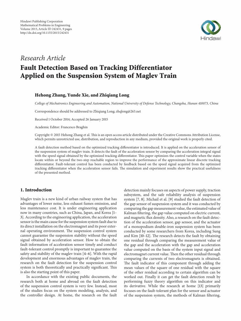
Figure 1 Suspension control system of the module
strong tracking filtering and full-dimension observer areapplied after the suspension control system is linearized at theequilibrium point And then the fault is detected by checkingthe parameters and states of system before and after the fault
In view of the existing methods this paper focuses on thefault detection for the acceleration sensor of the suspensionsystem in the maglev train If model-based fault detectionmethod [14] is employed the detection effect will be greatlydiscounted because the mathematical model of suspensionsystem cannot be obtained accurately If knowledge-basedfault detection method [15] is taken the suspension systemwould not be very applicable due to the lack of priorknowledge of fault Consider that many faults will affect themeasurement of signal (generally the inputoutput signal)and change some of their features in practical system Themethod based on processing the inputoutput signal analyzesthe features of the detectable signal such as the correlationfunction frequency spectrum higher-order statistics andautoregression moving average process By observing thechange of features of the signal or comparing the redundancysignal it can infer the fault model and then realize faultdetection By optimizing the approximate linear trackingdifferentiator proposed by Han and Yuan [16] (hereinafterreferred to as 119865119905119889) and extracting the speed signal as thereference signal with 119865119905119889 algorithm this paper compares thereference signal with the acceleration sensor signal And thenthe fault of the acceleration sensor is detected by the thresholdvalue that is set by introducing the Bayesian DecisionTheory[17 18] for comparison result The fault-tolerant control isperformed by introducing the speed signal acquired by theoptimized linear tracking differentiator when fault occurs
2 Analysis of the Structure and Problem of theSuspension Control System in Maglev Train
21 Structure of the Suspension Maglev train is an integratedelectromechanical system composed of vehicle structurebogie track suspension controller and suspension sensorgroup and so forth As shown in Figures 1-2 the four elec-tromagnets (EM) of suspension control system are controlledby two controllers The unit of PWM exerts ultimate voltageon the electromagnets Each controller corresponds to twoseries connected electromagnets Controller 1 and Controller
0
0
120574minus
120574+u = +r
u = minusr
O
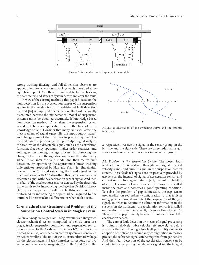
Figure 2 Illustration of the switching curve and the optimaltrajectory
2 respectively receive the signal of the sensor group on theleft side and the right side There are three redundancy gapsensors and one acceleration sensor in one sensor group
22 Problem of the Suspension System The closed loopfeedback control is realized through gap signal verticalvelocity signal and current signal in the suspension controlsystem These feedback signals are respectively provided bygap sensor the integral of signal of acceleration sensor andcurrent sensor In maglev train project the fault probabilityof current sensor is lower because the sensor is installedinside the crate and possesses a good operating conditionTo solve the problem of gap connection the gap sensoruses triplication redundancy configuration so that fault inone gap sensor would not affect the acquisition of the gapsignal In order to acquire the vibration information in thesuspension electromagnet the acceleration sensor is installedon the electromagnet As a result it is more likely to fail [6]Therefore this paper mainly targets the fault detection of theacceleration sensor
The core of fault detection by means of signal processingis to find a relatively stable velocity reference signal beforeand after the fault Having a low fault probability due to itsadoption of triplication redundancy configuration in maglevproject the reference signal can be required from gap sensorAnd then fault detection of the acceleration sensor can beconducted by comparing the reference signal and the integral
Mathematical Problems in Engineering 3
of the acceleration sensor signal In this paper the velocitysignal of system is acquired by using the tracking differentia-tor Tracking differentiator with obvious flutter phenomenonand requirement of high-frequency adjustment of controlvariable is unacceptable for the practical control systembecause the high-frequency change needs to consume muchenergy and the high-frequency perturbation of trackingsignal indicates the abrasion of mechanical deviceThereforethis paper aims at optimizing the parts that have overshooterror or flutter phenomenon on the basis of the approximatelinear tracking differentiator proposed by Han and Yuan [16]By optimizing the deviation of control algorithm whereverthe states locate within or beyond the two-step reachableregion the flutter problem can be solvedAnd an approximatelinear tracking differentiator (hereinafter referred to as 119865119905119889)that does not contain the square roots algorithm and whoseform is simple and whose implement action is easy can beacquired
3 An Optimized Approximate Linear TrackingDifferentiator Algorithm
According to part 2 the key to the fault detection of theacceleration sensor for the suspension system of maglevtrain is to obtain the efficient velocity signal as the referencesignal Gaining the differential signal rapidly and accuratelyand restraining the noise in the signal have always beenan important topic Tracking differentiator (TD) can trackthe input signal and extract of appropriate differential sig-nal effectively which make it increasingly popular amongresearchers Khalil and some other researchers [19 20]designed a linear high-gain differentiator which providesthe derivatives of signal from 1 to (119899 minus 1) The trackingdifferentiator based on bang-bang control is actually a kind ofsliding differentiator Researchers such as Levant [21ndash24] andUtkin [25 26] have done a series of studies on the featuresof sliding differentiator They applied this differentiator tofiltering sliding-mode control parameter estimation and soforth and have obtained certain achievements Han and Yuan[16] proposed a discrete tracking differentiator based on thesecond order time-optimal control system and applied it toactive-disturbance-rejection control (ADRC) [27] It solvesthe complex problems of disturbance observation trackingcontrol and parameter estimation better and has a goodrobust stability In the meantime Xie proposed a second-order nonlinear discrete tracking differentiator based on theresearch of Han that is able to amend its characteristic pointsand is flexible to applications And Xie applied this differen-tiator to the velocity and position detection of a permanentmagnet electrodynamicmaglev train system [28] To simplifythe discrete tracking differentiator Han [29] proposes a kindof approximate linear discrete tracking differentiator in hisbook Active-Disturbance-Rejection Controller CompensationTechnology taking the features of two-step reachable regionand the reversion of switching curve into considerationHowever the tracking trajectory obtained according to thefinal formula in this book has problems of overshoot andflutter which makes it difficult to promote and apply This
part discusses the simplification of the approximate linearand points out the disadvantage of the approximate linearformula in [29] Finally this part gives an optimized approx-imate linear discrete formula The simulation results showerror between the TD of Han and the two other differentlinear approximate formulas respectively
31 Synthesis Function of Second-OrderDiscrete Time-OptimalControl System In accordance with the optimal control the-ory the time-optimal control of the second-order integratorsystem with the starting point as the terminal one is bang-bang control [30] And themodel of the second-order systemcan be written as
1= 1199092
2= 119906 |119906| le 119903
(1)
The switching curve of the bang-bang control can be given by
Γ (1199091 1199092) = 1199091+1199092
100381610038161003816100381611990921003816100381610038161003816
2119903 (2)
Control strategy that is shown in Figure 2 can be defined as
119906 = minus119903 sgn (Γ (1199091 1199092)) (3)
When the second-order integrator system is dispersedsimply the system would generate unsatisfactory high-frequency flutter after it stabilizes It is a challenge to boththe study and application of rapid tracking differentiator Afurther research on the reasons for flutter is a must Theboundary characteristic curves of linear regions with thesecond-order discrete time-optimal control are presentedusing the method of the state back step by Han And bymeans of it Han designed a brilliant method that avoided theflutter According to the algorithm of the discrete trackingdifferentiator in document [29] it can be assumed that thediscrete step is ℎ any point on the phase plane is119872(119909
1 1199092)
and then the discretionary result of (1) is (4) And the controlforce 119906 is determined by (5) The algorithm (herein referredto as 119865ℎ119886119899) formula can be written as
1199091(119896) = 119909
1(119896) + ℎ119909
2(119896)
1199092(119896) = 119909
2(119896) + ℎ119906 (119896)
|119906 (119896)| le 119903 119896 = 0 1 2
(4)
Ω119903=
10038161003816100381610038161199091 + ℎ11990921003816100381610038161003816 le ℎ2119903 cap
10038161003816100381610038161199091 + 2ℎ11990921003816100381610038161003816 le ℎ2119903
if sdot 119872 sube Ω119903
119906 = minus1199091+ 2ℎ119909
2
ℎ2
else
119910 = 1199091+ ℎ1199092
119892 (1199091 1199092) = 1199092minus (
ℎ119903
2minus1
2radicℎ21199032 + 8119903
10038161003816100381610038161199101003816100381610038161003816) sgn (119910)
119906 = minus119903 sdot sat (119892 (1199091 1199092) ℎ119903)
end
(5)
4 Mathematical Problems in Engineering
Removing the ldquoif rdquo statement in formula (5) the formula canbe adapted as follows by using the sign function
119889 = 119903ℎ2 119886
0= ℎ1199092 119910 = 119909
1+ 1198860
1198861= radic119889 (119889 + 8
10038161003816100381610038161199101003816100381610038161003816)
1198862= 1198860+sign (119910) (119886
1minus 119889)
2
119878119910=(sign (119910 + 119889) minus sign (119910 minus 119889))
2
119886 = (1198860+ 119910 minus 119886
2) 119878119910+ 1198862
119878119886=(sign (119886 + 119889) minus sign (119886 minus 119889))
2
119865ℎ119886119899 = minus119903 (119886
119889minus sign (119886)) 119878
119886minus 119903 sign (119886)
(6)
Apparently formula (6) contains the square roots algo-rithm which complicated the whole algorithm and increasedthe calculationThis is inefficient for the practical engineeringapplication In formula (5) Ω
119903is the two-step reachable
region which is a rhombus circled by four points (minusℎ2119903 0)(minus3ℎ2119903 2ℎ119903) (ℎ2119903 0) and (3ℎ2119903 minus2ℎ119903) as shown in Figure 3
the region circled by blue line 119892(1199091 1199092) is the boundary
transfer function and sat(119909 120575) is the standard saturationfunction The sketch map of the switching curve two-stepreachable region and the optimal trajectory is shown inFigure 3
32 Boundary Simplification and Approximate Linear Rep-resentation Without considering the boundary layer thick-ness it can simplify the boundary and get the switching curveunder discretization as follows
Γ0(1199091 1199092) 1199091+1199092
100381610038161003816100381611990921003816100381610038161003816
2119903+1
2ℎ1199092= 0 (7)
In accordance with the method in document [16] the quasi-linear algorithm is expressed as follows
119889 = ℎ2119903 119911
1= 1199091+ ℎ1199092
1199112= 1199111+ ℎ1199092 119886 = 119909
1+1199092
100381610038161003816100381611990921003816100381610038161003816
2119903+1
2ℎ1199092
1198781=(sgn (119911
1+ 119889) minus sgn (119911
1minus 119889))
2
1198782=(sgn (119911
2+ 119889) minus sgn (119911
2minus 119889))
2
119878119888= 11987811198782 119880
119885= minus
1199112
ℎ2 119880
119886= minus119903 sgn (119886)
119906 = 119878119888119880119911+ (1 minus 119878
119888) 119880119886
(8)
0
0x2
x1
Figure 3 Illustration of the reachable area switching curve and theoptimal trajectory
And according to the book of Han [29] the approximate TDis expressed as follows
119889 = ℎ2119903 119886
0= ℎ1199092
119910 = 1199091+ 1198860 119911 = 119910 + 119886
0
119886 = 119910 +1198860(100381610038161003816100381611988601003816100381610038161003816 119889 minus 1)
2
119878119910=(sgn (119910 minus 119889) minus sgn (119910 + 119889))
2
119878119911=(sgn (119911 minus 119889) minus sgn (119911 + 119889))
2
119906 = minus119903 (119911 minus sign (119911) minus sign (119886) 119878119910119878119911+ sign (119911) + sign (119886))
(9)
To further discuss formula (9) a conclusion can be drawnthat if 119872(119909
1 1199092) on the phase plan is within the two-step
reachable region namely |119910| le 119889 cap |119911| le 119889 119872 sube Ω119903 then
it can obtain that 119878119910119878119911= 1 119906 = minus119903
119911 But the actual algorithm
should be 119906 = minus119911ℎ2 by computation when 119872(119909
1 1199092) is
within the two-step reachable region Besides taking thepoint beyond the two-step reachable region into accountnamely 119878
119910119878119885
= 1 119906 = minus119903(sgn(119911) + sgn(119886)) the actualreversion algorithm is 119906 = minus119903 sgn(119886) so naturally differencealso exists here Therefore the conclusion can be drawn thatthe approximate linear algorithm (9) in document [29] ispartially erred and the right algorithm should be formula (8)
According to the analysis of formula (9) there is aredundant sgn(119911) both within and beyond the reachableregion and factor 119889 is missing for the item with 119911 The correctformula is as follows
119906 = minus119903 (119911
119889minus sgn (119886) 119878
119910119878119911+ sgn (119886)) (10)
Mathematical Problems in Engineering 5x2
x1
10
5
0
minus5
minus10minus08 minus06 minus04 minus02 0 02 04 06 08
Fhan1
Fhan
Ftd
Figure 4 Illustration of trajectory of three different TD algorithms
The result now is the same as that of (8) and formula (9) canbe revised as
119889 = ℎ2119903 119886
0= ℎ1199092
119910 = 1199091+ 1198860 119911 = 119910 + 119886
0
119886 = 119910 +1198860(100381610038161003816100381611988601003816100381610038161003816 119889 minus 1)
2
119878119910=(sgn (119910 + 119889) minus sgn (119910 minus 119889))
2
119878119911=(sgn (119911 + 119889) minus sgn (119911 minus 119889))
2
119906 = minus119903 (119911
119889minus sgn (119886) 119878
119910119878119911+ sgn (119886))
(11)
Formula (11) is completely equal to formula (8) whichis a correction of formula (9) Thus this formula showsthe disadvantage of document [29] by Han and corrects theshortcoming
33 Comparison of the Numerical Simulation Result Tocompare the errors of the two approximates against the TD ofHan we can compare the phase path of a point on the phaseplane firstly and then study the difference with the trackinginput signal and differential signal
(1) The Time-Optimal Trajectory on the Phase PlaneTD algorithm of Han is formula (6) and here is expressed
as 119865ℎ119886119899 Its approximate algorithm before correction isformula (9) which is recorded as 119865ℎ1198861198991 And the newapproximate algorithm (11) is displayed as 119865119905119889 The result isas shown in Figure 4
As shown in Figure 4 algorithm 119865ℎ1198861198991 (formula (9))deviated from the switching curve with overshoot and wind-ing phenomenon which is largely different from 119865ℎ119886119899 Butalgorithm 119865119905119889 is slightly deviated from the switching curveand has slight deviation with algorithm 119865ℎ119886119899 According toFigure 3 the algorithm of 119865119905119889 that is the approximate one ofTD is a feasible linear approximate algorithm But formula(10) is largely deviated which is apparently disadvantaged
0 005 01 015 02 025
0
5
Time (s)
x1
Fhan1Fhan
Ftd
minus5
minus10
Figure 5 Illustration of the comparison of the tracking error ofinput signal
0 005 01 015 02 025
0
01
02
Time (s)
x1
Fhan1Fhan
Ftd
minus01
Figure 6 Illustration of the comparison differential error of theinput signal
(2) The following simulation is the comparison for threedifferent TD algorithms (119865ℎ1198861198991 119865ℎ119886119899 119865119905119889) by using a com-mon input signal to illustrate the ability of tracking inputsignal and extracting relevant differential signal of them
It is defined as follows input signal as V(119905) = sin(025120587119905)+120574(119905) sampling period as ℎ = 001 s rapid factor as 119903 = 120the original value as 119909
1(0) = 02 119909
2(0) = minus1 and 120574(119905) as the
evenly distributed white noise with intensity as 0001 Basedon the discrete model of (4) the analysis and comparison ofthe three algorithms119865ℎ119886119899 119865ℎ1198861198991 and119865119905119889 against the earliermentioned tracking error of sinusoidal signal and differentialerror of the obtained signal is as in Figures 5 and 6
As shown in Figure 5 the deviation of algorithm 119865ℎ1198861198991 islarger and flutter of it is severer while algorithm 119865119905119889 iscloser to119865ℎ119886119899 And as Figure 6 shows the approximate linearalgorithm 119865119905119889 is very close to algorithm 119865ℎ119886119899 and 119865ℎ1198861198991
has larger deviation and flutter phenomenon Under thecircumstances of input signal having noise the deviations ofboth the tracking signal and differential signal for 119865ℎ1198861198991are large To some extent the differential signal of algo-rithm 119865ℎ1198861198991 is unavailable in practical system In terms of
6 Mathematical Problems in Engineering
the plane phase trajectory the tracking error and the dif-ferential quality the approximate linear algorithm presentedin this paper is closer to algorithm 119865ℎ119886119899 proposed by Hanwhich is an appropriate improvement to the approximatelinear algorithm in [29] of Han
4 The Application of Optimized TD inthe Fault Detection of Acceleration Sensor
41 Simulation Analysis of Fault Detection A model of theelectromagnet of low-speed maglev train has been given inthe documents [30] Adopting the current loop feedback andusing the practical parameters the state equation can beshown
(119905) =
[[[[[
[
0 0 1 0
0 0 0 1
21437 30625 0 0
30625 21437 0 0
]]]]]
]
119909 (119905)
+
[[[[[
[
0 0
0 0
minus35178 minus05025
minus05025 minus35178
]]]]]
]
119906 (119905)
(12)
According to the optimal control theory the feedback controlalgorithm can be obtained as follows
119906 (119905) = 119870119909 (119905) = [
12188 0 265 minus19
0 12188 minus19 265] 119909 (119905) (13)
where the state vector is 119909(119905) = [1199091 119909211990931199094] and the
first two elements in the state vector respectively indicatethe variation of the gap on the left-side and right-side sensoragainst the steady-state value namely the gap deviation Andthe last two elements in the state vector respectively indicatethe vertical speed of train of the left-side and right-sidesensor All tracks of the maglev train during simulation aredeemed smooth
The two single electromagnets in the electromagnetmodule are symmetricalWithout loss of generality here takethe acceleration sensor of the left-side single electromagnethaving fault as an example to simulate In order to verifythe tracking and differential extraction ability in these threealgorithms the parameters in algorithms of119865ℎ119886119899119865ℎ1198861198991 and119865119905119889 are set with one accord
Figure 7 to Figure 9 demonstrate the simulation of theleft-side signal when system is fault-free Figure 7 showsthe gap deviation and the tracking status of three kindsof tracking differentiators Figure 8 displays comparison ofthe gap differential signal gained from three tracking differ-entiators and the acceleration integral signal And Figure 9displays the absolute 119863-value (residual for short) betweenthe gap differential signal obtained by the three trackingdifferentiators and the acceleration integral signal
As shown in Figures 7 8 and 9 the system is understable suspension when fault is free Since the characteristic
02 025 03 035 04 045 05
0
1
2
Gap
(m)
Time (s)
minus1
minus2
times10minus4
MeasurementFhan1Fhan
Ftd
Figure 7 Comparison between the left-side gap deviation and thetracking filtering value without fault
02 021 022 023 024 025 026 027 028 029 03
00005
0010015
002
Time (s)
Velo
city
(ms
)
Integral of accelerationFhan1Fhan
Ftd
minus0005minus001minus0015
Figure 8 Comparison between the gap differential value and theleft-side acceleration integral value without fault
of maglev train the gap deviation signal is included the whitenoise signal that is distributed evenly In other words thedifferential signals and gap signal must have signal-like noisewhich is not affected by external disturbance The simulationresults also indicate that 119865ℎ1198861198991 is very sensitive to noiseand it is unable to process the noise and further obtain thetracking and differential signal To some degree 119865ℎ1198861198991 is notapplicable in the maglev train system A conclusion can bedrawn that the tracking and differential extraction ability ofthe two tracking differentiators in algorithms 119865ℎ119886119899 and 119865119905119889are approximate And both of themhave a goodfiltering effecton the gap signal In addition their noise arising from gapdifferential is also within the minor magnitude
Figures 10 11 and 12 demonstrate the simulation resultsof left-side acceleration sensor when a fault has occurred at05 seconds (ie output as 0)
As can be seen from Figure 10 the system begins toshake and diverge when the left-side accelerations sensorfails But at the same time the tracking differentiator stillcan track and extract differential signal of the gap signalto a certain extent However the tracking and differentialextraction of noise signal from algorithm 119865ℎ1198861198991 is not goodaccording to the simulation results All the signals obtainedfrom 119865ℎ1198861198991 algorithm in this system are useless When theleft-side acceleration sensor fails the acceleration integralvalue remains the same and it makes gap differential valueand the gap signal shake and diverge which leads to bigger
Mathematical Problems in Engineering 7
02 022 024 026 028 030
0005
001
0015
002
Time (s)
Resid
ual e
rror
(ms
)
Fhan1FhanFtd
Figure 9 Comparison of the three left-side residuals without fault
045 05 055 06 065 07 075 08
0
2
4
Time (s)
Gap
(m)
MeasurementFhan1Fhan
Ftd
minus2
minus4
times10minus4
Figure 10 Comparison between the tracking filtering value and gapdeviation with acceleration sensor failure
05 1 15 2 25 3
0005
01015
Time (s)
Velo
city
(ms
)
Integral of accelerationFhan1Fhan
Ftd
minus005
minus01
minus02
minus015
Figure 11 Comparison between gap differential and left-side accel-eration integral value with acceleration sensor failure
05 1 15 2 25 30
002004006008
01012014
Time (s)
Resid
ual e
rror
(ms
)
Fhan1FhanFtd
Figure 12 Comparison of three residuals on the left side withacceleration sensor failure
residual As can be seen from the result if the threshold valueis set at 002 the fault can be detected at 052 seconds
42 Threshold Selection The selection of the earlier men-tioned threshold is largely subjective In order to improve theinstantaneity of fault detection and to decline the false alarmrate it is necessary to introduce an approach of thresholdselection that is practical and objective This paper calculatesthreshold based on the Bayesian Decision Theory [17] Thealgorithm is as follows
(1) calculation of the mean value and variance of theresidual in normal state
1205831198900=
1
1198731199081
1198731199081
sum
119894=1
119903 (119894) 1205902
0=
1
1198731199081
1198731199081
sum
119894=1
[119903(119894) minus 1205831198900]2
(14)
where 119903(119894) indicates the residual sequence in normalstate and119873
1199081indicates the data window length
(2) calculation of all types of statistical property of resid-ual when the system is running
120583119890=
1
1198731199081
1198731199081
sum
119894=1
119903 (119896 minus 119894)
1205902
0(119896) =
1
1198731199081
1198731199081
sum
119894=1
[119903(119896 minus 119894) minus 1205831198900]2
1205902
Π(119896) =
1
1198731199081
1198731199081
sum
119894=1
[119903(119896 minus 119894) minus 1205831198900]2
(15)
where 119903(119896 minus 1) indicates the residual sequence that iswaiting for detecting and119873
119908≻ 1198731199081
indicates the datawindow length
(3) decision content 119889 and threshold value 119905ℎ119903
119889119895(119896) =
1205902
119868(119896)
1205902
0
minus ln1205902
Π(119896)
1205902
0
minus 1
119889119895(119896)
le 2 ln(119873119908119875119905
(1 minus 119875119905)) fault-free
ge 2 ln(119873119908119875119905
(1 minus 119875119905)) fault
(16)
where 119875119905is the prior probability when system is fault-
free According to the experience of practical projectit can be chosen as 119875
119905= 08 Figure 13 displays the
result of threshold by the method mentioned abovewhen it is applied to the residual data
As can be seen from the simulation result of faultdetection in part 41 algorithm119865ℎ1198861198991 is sensitive to the high-frequency noise signal And it cannot process noise signalto track or extract the differential signal of the system Asa result only 119865119905119889 algorithm has been adopted to do thesimulation analysis when decision content and thresholdvalue are analyzed As shown in the simulation diagramtaking 119875
119905= 08 the fault on the left-side acceleration sensor
can be detected at 052 seconds
8 Mathematical Problems in Engineering
0 01 02 03 04 05 06 07 080
5
10
15
Time (s)
Decision variableThreshold
dan
d thr
Figure 13 Decision content and threshold value
5 Fault-Tolerant Control ofAcceleration Sensor
As can be seen from part 2 it is much likely to breakdown in acceleration sensor in the suspension control systemof maglev train Fault-tolerant control can be conductedby replacing the acceleration integral signal with the gapdifferential signal extracted by the optimized approximatelinear tracking differentiator when the acceleration sensorfails The specific schematic diagram of the scheme is shownin Figures 1ndash5 where gap differential 1199111015840 is the gap signalprocessed by differentiator and acceleration integrated signalint 119886 is acceleration signal processed by integrator and decisioncontent 119889 and threshold value 119905ℎ119903 are processed by the faultdetection unit based on the difference between 119911
1015840 and int 119886Signal 119904 is obtained based on the relationship between 119889
and 119905ℎ119903 The controller then makes the choice between 1199111015840
and int 119886 according to the difference of 119904 int 119886 is regardedas the velocity feedback when system is normal but whenfault is detected in accelerometer by fault detection unit1199111015840 is regarded as the velocity feedback Thus fault-tolerantcontrol of accelerometer fault is realized Figure 14 shows theintroduction of the speed signal 1199111015840 obtained from the trackingdifferentiator into the closed loop feedback control after theacceleration sensor fails during the experiment The resultshows that the introduction of the speed signal obtainedfrom the tracking differentiator into the feedback control canstabilize the system which is fault-tolerant control
Figure 15 shows the ultimate gap deviation curve afterintroducing the speed signal 119911
1015840 obtained by 119865119905119889 algo-rithm when the acceleration sensor fails during experimentFigure 16 shows the ultimate absolute stable gap value (thesuspension gap is between 453mm and 454mm whenthe maglev train is in stable state) after introducing thefault-tolerant control During the experiment the closureof acceleration sensor power is performed to simulate thefault of acceleration sensor And then speed signal 1199111015840 isintroduced at the first second when the system detects faultThe experimental result shows that the introduction of thespeed signal acquired from the tracking differentiator into thefeedback control can make system stable
Electromagnet
Accelerometer
Gap sensor
FDD
Integral
TD
ChopperCurrentsensor
Controller
Kc
Kp
K
Switch
z
z998400
i
u
s
a inta
Figure 14 Schematic diagram of the fault detection and fault-tolerant control scheme for acceleration sensor
08 09 1 11 12 13 14 15 16 17 18
024
Time (s)
Gap
erro
r (m
) Measurement
Ftd
times10minus4
minus2
minus4
minus6
Figure 15 The experimental curve of the actual gap error afterintroducing the fault-tolerant control when acceleration sensor fails
1 12 14 16 18 2 224525
453
4535
454
4545
Time (s)
Gap
(mm
)
Gap
Figure 16 The experimental curve of the actual absolute gap afterintroducing the fault-tolerant control when acceleration sensor fails
6 Conclusion
This paper focuses on the fault detection of the accelerationsensor for the suspension system of maglev train Thepaper studies the approximate linear tracking differentiatorproposed by Han during acquiring the speed reference signaland presents a new approximate linear tracking differen-tiator based on the correction of the disadvantages of thisdifferentiator Numerical simulation of given signal showsthat 119865119905119889 algorithm with simple form (without the squareroots algorithm) can quickly track an input signal without
Mathematical Problems in Engineering 9
chattering and can produce a good differential signal whichis easy to realize in practical application According to theexperiment fault-tolerant control by using the speed signalobtained from 119865119905119889 algorithm when the acceleration sensorfails is feasible
Conflict of Interests
The authors declare that there is no conflict of interestsregarding the publication of this paper
References
[1] Z-R Liu ldquoCommercialization of HSST an access line of for the2005 world exposition in Aichi Japanrdquo Converter Technology ampElectric Traction vol 3 no 1 pp 50ndash52 2005
[2] R-J Wai J-D Lee and K-L Chuang ldquoReal-time PID controlstrategy for maglev transportation system via particle swarmoptimizationrdquo IEEE Transactions on Industrial Electronics vol58 no 2 pp 629ndash646 2011
[3] E Kong J-S Song B-B Kang and S Na ldquoDynamic responseand robust control of coupled maglev vehicle and guidewaysystemrdquo Journal of Sound and Vibration vol 330 no 25 pp6237ndash6253 2011
[4] S Banerjee M K Sarkar P K Biswas R Bhaduri and PSarkar ldquoA review note on different components of simpleelectromagnetic levitation systemsrdquo IETE Technical Review vol28 no 3 pp 256ndash264 2011
[5] Y Li G He and J Li ldquoNonlinear robust observer-based faultdetection for networked suspension control system of maglevtrainrdquoMathematical Problems in Engineering vol 2013 ArticleID 713560 7 pages 2013
[6] Y Li J Li G Zhang and W-J Tian ldquoDisturbance decoupledfault diagnosis for sensor fault of maglev suspension systemrdquoJournal of Central South University vol 20 no 6 pp 1545ndash15512013
[7] Z Q Long Z Q Lv S Huan and W S Chang ldquoAnalysis anddesign in safeties and reliabilities of the suspension systemof Maglev trainrdquo in Proceedings of the 5th World Congress onIntelligent Control and Automation (WCICA rsquo04) pp 1819ndash1823HangZhou China June 2004
[8] Z-Q Long Y Cai and J Ye ldquoAnalysis of the reliabilities ofmaglev train power system with DFTAmethodrdquo in Proceedingsof the 19th International Conference on Magnetically LevitatedSystems and Linear Drives (MAGLEV rsquo2006) pp 449ndash502Dresden Germany September 2006
[9] K Michail A Zolotas R Goodall and J Pearson ldquoFault toler-ant control for EMS systems with sensor failurerdquo in Proceedingsof the 17th Mediterranean Conference on Control Automationpp 712ndash717 Thessaloniki Greece June 2009
[10] H K Sung S H Lee and Z Bien ldquoDesign and implementationof a fault tolerant controller for EMS systemsrdquoMechatronics vol15 no 10 pp 1253ndash1272 2005
[11] H K Sung D S Kim H J Cho M H Yoo B S Kim andJ M Lee ldquoFault tolerant control of electromagnetic levitationsystemrdquo in Proceedings of the 18thMagnetically Levitated Systemand Linear Drives Conference (MAGLEV rsquo04) pp 676ndash6882004
[12] H-J Kim C-K Kim and S Kwon ldquoDesign of a fault-tolerantlevitation controller formagnetic levitation vehiclerdquo in Proceed-ings of the International Conference on Electrical Machines andSystems (ICEMS rsquo07) pp 1977ndash1980 October 2007
[13] Z Q Long S Xue Z-Z Zhang and Y-D Xie ldquoA new strategyof active fault-tolerant control for suspension system of maglevtrainrdquo in Proceedings of the IEEE International Conference onAutomation and Logistics (ICAL rsquo07) pp 88ndash94 August 2007
[14] J Chen and R-J PattonRobustModel-Based Fault Detection forDynamic Systems Kluwer Academic Publishers Boston MassUSA 1999
[15] P-M Frank ldquoFault diagnosis in dynamic systems using analyti-cal and knowledge-based redundancymdasha survey and some newresultsrdquo Automatica vol 26 no 3 pp 459ndash474 1990
[16] J Q Han and L L Yuan ldquoThe discrete form of a tracking-differentiatorrdquo Journal of Systems Science and MathematicalSciences vol 19 no 3 pp 268ndash273 1999
[17] T Bayes ldquoAn essay toward solving a problem in the doctrineof chancesrdquo Philosophical Transactions of the Royal Society ofLondon vol 53 pp 370ndash418 1763
[18] J W Sheppard and M A Kaufman ldquoA Bayesian approach todiagnosis and prognosis using built-in testrdquo IEEE Transactionson Instrumentation and Measurement vol 54 no 3 pp 1003ndash1018 2005
[19] H-K Khalil ldquoRobust servomechanism output feedback con-trollers for feedback linearizable systemsrdquo Automatica vol 30no 10 pp 1587ndash1599 1994
[20] A N Atassi and H K Khalil ldquoSeparation results for thestabilization of nonlinear systems using different high-gainobserver designsrdquo Systems amp Control Letters vol 39 no 3 pp183ndash191 2000
[21] A Levant ldquoRobust exact differentiation via sliding modetechniquerdquo Automatica vol 34 no 3 pp 379ndash384 1998
[22] A Levant ldquoHigher-order sliding modes differentiation andoutput-feedback controlrdquo International Journal of Control vol76 no 9-10 pp 924ndash941 2003
[23] A Levant ldquoSliding order and sliding accuracy in sliding modecontrolrdquo International Journal of Control vol 58 no 6 pp 1247ndash1263 1993
[24] A Levant ldquoPrinciples of 2-sliding mode designrdquo Automaticavol 43 no 4 pp 576ndash586 2007
[25] V-I Utkin J Guldner and J Shi Sliding Mode in Control inElectromechanical Systems Taylor amp Francis London UK 1999
[26] V I Utkin and A S Poznyak ldquoAdaptive sliding mode controlwith application to super-twist algorithm equivalent controlmethodrdquo Automatica vol 49 no 1 pp 39ndash47 2013
[27] J-Q Han ldquoFromPID technique to active disturbances rejectioncontrol techniquerdquo Control Engineering of China vol 19 no 3pp 13ndash18 2002
[28] Y D Xie Y G Li Z Q Long and C C Dai ldquoDiscrete second-order nonlinear tracking-differentiator based on boundarycharacteristic curves and variable characteristic points and itsapplication to velocity and position detection systemrdquo ActaAutomatica Sinica vol 40 no 5 pp 952ndash964 2014
[29] J-Q Han Active Disturbance Rejection Control The Techniquefor Estimating and Compensating the Uncertainties NationalDenfence Industry Press 2008
[30] D-S Liu Research on the Module Suspension Control Problemof the EMS Low-Speed Maglev National University of DefenseTechnology Changsha China 2006
Submit your manuscripts athttpwwwhindawicom
Hindawi Publishing Corporationhttpwwwhindawicom Volume 2014
MathematicsJournal of
Hindawi Publishing Corporationhttpwwwhindawicom Volume 2014
Mathematical Problems in Engineering
Hindawi Publishing Corporationhttpwwwhindawicom
Differential EquationsInternational Journal of
Volume 2014
Applied MathematicsJournal of
Hindawi Publishing Corporationhttpwwwhindawicom Volume 2014
Probability and StatisticsHindawi Publishing Corporationhttpwwwhindawicom Volume 2014
Journal of
Hindawi Publishing Corporationhttpwwwhindawicom Volume 2014
Mathematical PhysicsAdvances in
Complex AnalysisJournal of
Hindawi Publishing Corporationhttpwwwhindawicom Volume 2014
OptimizationJournal of
Hindawi Publishing Corporationhttpwwwhindawicom Volume 2014
CombinatoricsHindawi Publishing Corporationhttpwwwhindawicom Volume 2014
International Journal of
Hindawi Publishing Corporationhttpwwwhindawicom Volume 2014
Operations ResearchAdvances in
Journal of
Hindawi Publishing Corporationhttpwwwhindawicom Volume 2014
Function Spaces
Abstract and Applied AnalysisHindawi Publishing Corporationhttpwwwhindawicom Volume 2014
International Journal of Mathematics and Mathematical Sciences
Hindawi Publishing Corporationhttpwwwhindawicom Volume 2014
The Scientific World JournalHindawi Publishing Corporation httpwwwhindawicom Volume 2014
Hindawi Publishing Corporationhttpwwwhindawicom Volume 2014
Algebra
Discrete Dynamics in Nature and Society
Hindawi Publishing Corporationhttpwwwhindawicom Volume 2014
Hindawi Publishing Corporationhttpwwwhindawicom Volume 2014
Decision SciencesAdvances in
Discrete MathematicsJournal of
Hindawi Publishing Corporationhttpwwwhindawicom
Volume 2014 Hindawi Publishing Corporationhttpwwwhindawicom Volume 2014
Stochastic AnalysisInternational Journal of
2 Mathematical Problems in Engineering
Bogie
Track
Susp
ensio
n se
nsor
gro
up 1
Gap Gap
Controller 1 Controller 2
EM 1 EM 2 EM 3 EM 4
PWM PWM
Susp
ensio
n se
nsor
gro
up 2
u i u i
c1(t) c2(t)
c1 c2
12
cc
Figure 1 Suspension control system of the module
strong tracking filtering and full-dimension observer areapplied after the suspension control system is linearized at theequilibrium point And then the fault is detected by checkingthe parameters and states of system before and after the fault
In view of the existing methods this paper focuses on thefault detection for the acceleration sensor of the suspensionsystem in the maglev train If model-based fault detectionmethod [14] is employed the detection effect will be greatlydiscounted because the mathematical model of suspensionsystem cannot be obtained accurately If knowledge-basedfault detection method [15] is taken the suspension systemwould not be very applicable due to the lack of priorknowledge of fault Consider that many faults will affect themeasurement of signal (generally the inputoutput signal)and change some of their features in practical system Themethod based on processing the inputoutput signal analyzesthe features of the detectable signal such as the correlationfunction frequency spectrum higher-order statistics andautoregression moving average process By observing thechange of features of the signal or comparing the redundancysignal it can infer the fault model and then realize faultdetection By optimizing the approximate linear trackingdifferentiator proposed by Han and Yuan [16] (hereinafterreferred to as 119865119905119889) and extracting the speed signal as thereference signal with 119865119905119889 algorithm this paper compares thereference signal with the acceleration sensor signal And thenthe fault of the acceleration sensor is detected by the thresholdvalue that is set by introducing the Bayesian DecisionTheory[17 18] for comparison result The fault-tolerant control isperformed by introducing the speed signal acquired by theoptimized linear tracking differentiator when fault occurs
2 Analysis of the Structure and Problem of theSuspension Control System in Maglev Train
21 Structure of the Suspension Maglev train is an integratedelectromechanical system composed of vehicle structurebogie track suspension controller and suspension sensorgroup and so forth As shown in Figures 1-2 the four elec-tromagnets (EM) of suspension control system are controlledby two controllers The unit of PWM exerts ultimate voltageon the electromagnets Each controller corresponds to twoseries connected electromagnets Controller 1 and Controller
0
0
120574minus
120574+u = +r
u = minusr
O
Figure 2 Illustration of the switching curve and the optimaltrajectory
2 respectively receive the signal of the sensor group on theleft side and the right side There are three redundancy gapsensors and one acceleration sensor in one sensor group
22 Problem of the Suspension System The closed loopfeedback control is realized through gap signal verticalvelocity signal and current signal in the suspension controlsystem These feedback signals are respectively provided bygap sensor the integral of signal of acceleration sensor andcurrent sensor In maglev train project the fault probabilityof current sensor is lower because the sensor is installedinside the crate and possesses a good operating conditionTo solve the problem of gap connection the gap sensoruses triplication redundancy configuration so that fault inone gap sensor would not affect the acquisition of the gapsignal In order to acquire the vibration information in thesuspension electromagnet the acceleration sensor is installedon the electromagnet As a result it is more likely to fail [6]Therefore this paper mainly targets the fault detection of theacceleration sensor
The core of fault detection by means of signal processingis to find a relatively stable velocity reference signal beforeand after the fault Having a low fault probability due to itsadoption of triplication redundancy configuration in maglevproject the reference signal can be required from gap sensorAnd then fault detection of the acceleration sensor can beconducted by comparing the reference signal and the integral
Mathematical Problems in Engineering 3
of the acceleration sensor signal In this paper the velocitysignal of system is acquired by using the tracking differentia-tor Tracking differentiator with obvious flutter phenomenonand requirement of high-frequency adjustment of controlvariable is unacceptable for the practical control systembecause the high-frequency change needs to consume muchenergy and the high-frequency perturbation of trackingsignal indicates the abrasion of mechanical deviceThereforethis paper aims at optimizing the parts that have overshooterror or flutter phenomenon on the basis of the approximatelinear tracking differentiator proposed by Han and Yuan [16]By optimizing the deviation of control algorithm whereverthe states locate within or beyond the two-step reachableregion the flutter problem can be solvedAnd an approximatelinear tracking differentiator (hereinafter referred to as 119865119905119889)that does not contain the square roots algorithm and whoseform is simple and whose implement action is easy can beacquired
3 An Optimized Approximate Linear TrackingDifferentiator Algorithm
According to part 2 the key to the fault detection of theacceleration sensor for the suspension system of maglevtrain is to obtain the efficient velocity signal as the referencesignal Gaining the differential signal rapidly and accuratelyand restraining the noise in the signal have always beenan important topic Tracking differentiator (TD) can trackthe input signal and extract of appropriate differential sig-nal effectively which make it increasingly popular amongresearchers Khalil and some other researchers [19 20]designed a linear high-gain differentiator which providesthe derivatives of signal from 1 to (119899 minus 1) The trackingdifferentiator based on bang-bang control is actually a kind ofsliding differentiator Researchers such as Levant [21ndash24] andUtkin [25 26] have done a series of studies on the featuresof sliding differentiator They applied this differentiator tofiltering sliding-mode control parameter estimation and soforth and have obtained certain achievements Han and Yuan[16] proposed a discrete tracking differentiator based on thesecond order time-optimal control system and applied it toactive-disturbance-rejection control (ADRC) [27] It solvesthe complex problems of disturbance observation trackingcontrol and parameter estimation better and has a goodrobust stability In the meantime Xie proposed a second-order nonlinear discrete tracking differentiator based on theresearch of Han that is able to amend its characteristic pointsand is flexible to applications And Xie applied this differen-tiator to the velocity and position detection of a permanentmagnet electrodynamicmaglev train system [28] To simplifythe discrete tracking differentiator Han [29] proposes a kindof approximate linear discrete tracking differentiator in hisbook Active-Disturbance-Rejection Controller CompensationTechnology taking the features of two-step reachable regionand the reversion of switching curve into considerationHowever the tracking trajectory obtained according to thefinal formula in this book has problems of overshoot andflutter which makes it difficult to promote and apply This
part discusses the simplification of the approximate linearand points out the disadvantage of the approximate linearformula in [29] Finally this part gives an optimized approx-imate linear discrete formula The simulation results showerror between the TD of Han and the two other differentlinear approximate formulas respectively
31 Synthesis Function of Second-OrderDiscrete Time-OptimalControl System In accordance with the optimal control the-ory the time-optimal control of the second-order integratorsystem with the starting point as the terminal one is bang-bang control [30] And themodel of the second-order systemcan be written as
1= 1199092
2= 119906 |119906| le 119903
(1)
The switching curve of the bang-bang control can be given by
Γ (1199091 1199092) = 1199091+1199092
100381610038161003816100381611990921003816100381610038161003816
2119903 (2)
Control strategy that is shown in Figure 2 can be defined as
119906 = minus119903 sgn (Γ (1199091 1199092)) (3)
When the second-order integrator system is dispersedsimply the system would generate unsatisfactory high-frequency flutter after it stabilizes It is a challenge to boththe study and application of rapid tracking differentiator Afurther research on the reasons for flutter is a must Theboundary characteristic curves of linear regions with thesecond-order discrete time-optimal control are presentedusing the method of the state back step by Han And bymeans of it Han designed a brilliant method that avoided theflutter According to the algorithm of the discrete trackingdifferentiator in document [29] it can be assumed that thediscrete step is ℎ any point on the phase plane is119872(119909
1 1199092)
and then the discretionary result of (1) is (4) And the controlforce 119906 is determined by (5) The algorithm (herein referredto as 119865ℎ119886119899) formula can be written as
1199091(119896) = 119909
1(119896) + ℎ119909
2(119896)
1199092(119896) = 119909
2(119896) + ℎ119906 (119896)
|119906 (119896)| le 119903 119896 = 0 1 2
(4)
Ω119903=
10038161003816100381610038161199091 + ℎ11990921003816100381610038161003816 le ℎ2119903 cap
10038161003816100381610038161199091 + 2ℎ11990921003816100381610038161003816 le ℎ2119903
if sdot 119872 sube Ω119903
119906 = minus1199091+ 2ℎ119909
2
ℎ2
else
119910 = 1199091+ ℎ1199092
119892 (1199091 1199092) = 1199092minus (
ℎ119903
2minus1
2radicℎ21199032 + 8119903
10038161003816100381610038161199101003816100381610038161003816) sgn (119910)
119906 = minus119903 sdot sat (119892 (1199091 1199092) ℎ119903)
end
(5)
4 Mathematical Problems in Engineering
Removing the ldquoif rdquo statement in formula (5) the formula canbe adapted as follows by using the sign function
119889 = 119903ℎ2 119886
0= ℎ1199092 119910 = 119909
1+ 1198860
1198861= radic119889 (119889 + 8
10038161003816100381610038161199101003816100381610038161003816)
1198862= 1198860+sign (119910) (119886
1minus 119889)
2
119878119910=(sign (119910 + 119889) minus sign (119910 minus 119889))
2
119886 = (1198860+ 119910 minus 119886
2) 119878119910+ 1198862
119878119886=(sign (119886 + 119889) minus sign (119886 minus 119889))
2
119865ℎ119886119899 = minus119903 (119886
119889minus sign (119886)) 119878
119886minus 119903 sign (119886)
(6)
Apparently formula (6) contains the square roots algo-rithm which complicated the whole algorithm and increasedthe calculationThis is inefficient for the practical engineeringapplication In formula (5) Ω
119903is the two-step reachable
region which is a rhombus circled by four points (minusℎ2119903 0)(minus3ℎ2119903 2ℎ119903) (ℎ2119903 0) and (3ℎ2119903 minus2ℎ119903) as shown in Figure 3
the region circled by blue line 119892(1199091 1199092) is the boundary
transfer function and sat(119909 120575) is the standard saturationfunction The sketch map of the switching curve two-stepreachable region and the optimal trajectory is shown inFigure 3
32 Boundary Simplification and Approximate Linear Rep-resentation Without considering the boundary layer thick-ness it can simplify the boundary and get the switching curveunder discretization as follows
Γ0(1199091 1199092) 1199091+1199092
100381610038161003816100381611990921003816100381610038161003816
2119903+1
2ℎ1199092= 0 (7)
In accordance with the method in document [16] the quasi-linear algorithm is expressed as follows
119889 = ℎ2119903 119911
1= 1199091+ ℎ1199092
1199112= 1199111+ ℎ1199092 119886 = 119909
1+1199092
100381610038161003816100381611990921003816100381610038161003816
2119903+1
2ℎ1199092
1198781=(sgn (119911
1+ 119889) minus sgn (119911
1minus 119889))
2
1198782=(sgn (119911
2+ 119889) minus sgn (119911
2minus 119889))
2
119878119888= 11987811198782 119880
119885= minus
1199112
ℎ2 119880
119886= minus119903 sgn (119886)
119906 = 119878119888119880119911+ (1 minus 119878
119888) 119880119886
(8)
0
0x2
x1
Figure 3 Illustration of the reachable area switching curve and theoptimal trajectory
And according to the book of Han [29] the approximate TDis expressed as follows
119889 = ℎ2119903 119886
0= ℎ1199092
119910 = 1199091+ 1198860 119911 = 119910 + 119886
0
119886 = 119910 +1198860(100381610038161003816100381611988601003816100381610038161003816 119889 minus 1)
2
119878119910=(sgn (119910 minus 119889) minus sgn (119910 + 119889))
2
119878119911=(sgn (119911 minus 119889) minus sgn (119911 + 119889))
2
119906 = minus119903 (119911 minus sign (119911) minus sign (119886) 119878119910119878119911+ sign (119911) + sign (119886))
(9)
To further discuss formula (9) a conclusion can be drawnthat if 119872(119909
1 1199092) on the phase plan is within the two-step
reachable region namely |119910| le 119889 cap |119911| le 119889 119872 sube Ω119903 then
it can obtain that 119878119910119878119911= 1 119906 = minus119903
119911 But the actual algorithm
should be 119906 = minus119911ℎ2 by computation when 119872(119909
1 1199092) is
within the two-step reachable region Besides taking thepoint beyond the two-step reachable region into accountnamely 119878
119910119878119885
= 1 119906 = minus119903(sgn(119911) + sgn(119886)) the actualreversion algorithm is 119906 = minus119903 sgn(119886) so naturally differencealso exists here Therefore the conclusion can be drawn thatthe approximate linear algorithm (9) in document [29] ispartially erred and the right algorithm should be formula (8)
According to the analysis of formula (9) there is aredundant sgn(119911) both within and beyond the reachableregion and factor 119889 is missing for the item with 119911 The correctformula is as follows
119906 = minus119903 (119911
119889minus sgn (119886) 119878
119910119878119911+ sgn (119886)) (10)
Mathematical Problems in Engineering 5x2
x1
10
5
0
minus5
minus10minus08 minus06 minus04 minus02 0 02 04 06 08
Fhan1
Fhan
Ftd
Figure 4 Illustration of trajectory of three different TD algorithms
The result now is the same as that of (8) and formula (9) canbe revised as
119889 = ℎ2119903 119886
0= ℎ1199092
119910 = 1199091+ 1198860 119911 = 119910 + 119886
0
119886 = 119910 +1198860(100381610038161003816100381611988601003816100381610038161003816 119889 minus 1)
2
119878119910=(sgn (119910 + 119889) minus sgn (119910 minus 119889))
2
119878119911=(sgn (119911 + 119889) minus sgn (119911 minus 119889))
2
119906 = minus119903 (119911
119889minus sgn (119886) 119878
119910119878119911+ sgn (119886))
(11)
Formula (11) is completely equal to formula (8) whichis a correction of formula (9) Thus this formula showsthe disadvantage of document [29] by Han and corrects theshortcoming
33 Comparison of the Numerical Simulation Result Tocompare the errors of the two approximates against the TD ofHan we can compare the phase path of a point on the phaseplane firstly and then study the difference with the trackinginput signal and differential signal
(1) The Time-Optimal Trajectory on the Phase PlaneTD algorithm of Han is formula (6) and here is expressed
as 119865ℎ119886119899 Its approximate algorithm before correction isformula (9) which is recorded as 119865ℎ1198861198991 And the newapproximate algorithm (11) is displayed as 119865119905119889 The result isas shown in Figure 4
As shown in Figure 4 algorithm 119865ℎ1198861198991 (formula (9))deviated from the switching curve with overshoot and wind-ing phenomenon which is largely different from 119865ℎ119886119899 Butalgorithm 119865119905119889 is slightly deviated from the switching curveand has slight deviation with algorithm 119865ℎ119886119899 According toFigure 3 the algorithm of 119865119905119889 that is the approximate one ofTD is a feasible linear approximate algorithm But formula(10) is largely deviated which is apparently disadvantaged
0 005 01 015 02 025
0
5
Time (s)
x1
Fhan1Fhan
Ftd
minus5
minus10
Figure 5 Illustration of the comparison of the tracking error ofinput signal
0 005 01 015 02 025
0
01
02
Time (s)
x1
Fhan1Fhan
Ftd
minus01
Figure 6 Illustration of the comparison differential error of theinput signal
(2) The following simulation is the comparison for threedifferent TD algorithms (119865ℎ1198861198991 119865ℎ119886119899 119865119905119889) by using a com-mon input signal to illustrate the ability of tracking inputsignal and extracting relevant differential signal of them
It is defined as follows input signal as V(119905) = sin(025120587119905)+120574(119905) sampling period as ℎ = 001 s rapid factor as 119903 = 120the original value as 119909
1(0) = 02 119909
2(0) = minus1 and 120574(119905) as the
evenly distributed white noise with intensity as 0001 Basedon the discrete model of (4) the analysis and comparison ofthe three algorithms119865ℎ119886119899 119865ℎ1198861198991 and119865119905119889 against the earliermentioned tracking error of sinusoidal signal and differentialerror of the obtained signal is as in Figures 5 and 6
As shown in Figure 5 the deviation of algorithm 119865ℎ1198861198991 islarger and flutter of it is severer while algorithm 119865119905119889 iscloser to119865ℎ119886119899 And as Figure 6 shows the approximate linearalgorithm 119865119905119889 is very close to algorithm 119865ℎ119886119899 and 119865ℎ1198861198991
has larger deviation and flutter phenomenon Under thecircumstances of input signal having noise the deviations ofboth the tracking signal and differential signal for 119865ℎ1198861198991are large To some extent the differential signal of algo-rithm 119865ℎ1198861198991 is unavailable in practical system In terms of
6 Mathematical Problems in Engineering
the plane phase trajectory the tracking error and the dif-ferential quality the approximate linear algorithm presentedin this paper is closer to algorithm 119865ℎ119886119899 proposed by Hanwhich is an appropriate improvement to the approximatelinear algorithm in [29] of Han
4 The Application of Optimized TD inthe Fault Detection of Acceleration Sensor
41 Simulation Analysis of Fault Detection A model of theelectromagnet of low-speed maglev train has been given inthe documents [30] Adopting the current loop feedback andusing the practical parameters the state equation can beshown
(119905) =
[[[[[
[
0 0 1 0
0 0 0 1
21437 30625 0 0
30625 21437 0 0
]]]]]
]
119909 (119905)
+
[[[[[
[
0 0
0 0
minus35178 minus05025
minus05025 minus35178
]]]]]
]
119906 (119905)
(12)
According to the optimal control theory the feedback controlalgorithm can be obtained as follows
119906 (119905) = 119870119909 (119905) = [
12188 0 265 minus19
0 12188 minus19 265] 119909 (119905) (13)
where the state vector is 119909(119905) = [1199091 119909211990931199094] and the
first two elements in the state vector respectively indicatethe variation of the gap on the left-side and right-side sensoragainst the steady-state value namely the gap deviation Andthe last two elements in the state vector respectively indicatethe vertical speed of train of the left-side and right-sidesensor All tracks of the maglev train during simulation aredeemed smooth
The two single electromagnets in the electromagnetmodule are symmetricalWithout loss of generality here takethe acceleration sensor of the left-side single electromagnethaving fault as an example to simulate In order to verifythe tracking and differential extraction ability in these threealgorithms the parameters in algorithms of119865ℎ119886119899119865ℎ1198861198991 and119865119905119889 are set with one accord
Figure 7 to Figure 9 demonstrate the simulation of theleft-side signal when system is fault-free Figure 7 showsthe gap deviation and the tracking status of three kindsof tracking differentiators Figure 8 displays comparison ofthe gap differential signal gained from three tracking differ-entiators and the acceleration integral signal And Figure 9displays the absolute 119863-value (residual for short) betweenthe gap differential signal obtained by the three trackingdifferentiators and the acceleration integral signal
As shown in Figures 7 8 and 9 the system is understable suspension when fault is free Since the characteristic
02 025 03 035 04 045 05
0
1
2
Gap
(m)
Time (s)
minus1
minus2
times10minus4
MeasurementFhan1Fhan
Ftd
Figure 7 Comparison between the left-side gap deviation and thetracking filtering value without fault
02 021 022 023 024 025 026 027 028 029 03
00005
0010015
002
Time (s)
Velo
city
(ms
)
Integral of accelerationFhan1Fhan
Ftd
minus0005minus001minus0015
Figure 8 Comparison between the gap differential value and theleft-side acceleration integral value without fault
of maglev train the gap deviation signal is included the whitenoise signal that is distributed evenly In other words thedifferential signals and gap signal must have signal-like noisewhich is not affected by external disturbance The simulationresults also indicate that 119865ℎ1198861198991 is very sensitive to noiseand it is unable to process the noise and further obtain thetracking and differential signal To some degree 119865ℎ1198861198991 is notapplicable in the maglev train system A conclusion can bedrawn that the tracking and differential extraction ability ofthe two tracking differentiators in algorithms 119865ℎ119886119899 and 119865119905119889are approximate And both of themhave a goodfiltering effecton the gap signal In addition their noise arising from gapdifferential is also within the minor magnitude
Figures 10 11 and 12 demonstrate the simulation resultsof left-side acceleration sensor when a fault has occurred at05 seconds (ie output as 0)
As can be seen from Figure 10 the system begins toshake and diverge when the left-side accelerations sensorfails But at the same time the tracking differentiator stillcan track and extract differential signal of the gap signalto a certain extent However the tracking and differentialextraction of noise signal from algorithm 119865ℎ1198861198991 is not goodaccording to the simulation results All the signals obtainedfrom 119865ℎ1198861198991 algorithm in this system are useless When theleft-side acceleration sensor fails the acceleration integralvalue remains the same and it makes gap differential valueand the gap signal shake and diverge which leads to bigger
Mathematical Problems in Engineering 7
02 022 024 026 028 030
0005
001
0015
002
Time (s)
Resid
ual e
rror
(ms
)
Fhan1FhanFtd
Figure 9 Comparison of the three left-side residuals without fault
045 05 055 06 065 07 075 08
0
2
4
Time (s)
Gap
(m)
MeasurementFhan1Fhan
Ftd
minus2
minus4
times10minus4
Figure 10 Comparison between the tracking filtering value and gapdeviation with acceleration sensor failure
05 1 15 2 25 3
0005
01015
Time (s)
Velo
city
(ms
)
Integral of accelerationFhan1Fhan
Ftd
minus005
minus01
minus02
minus015
Figure 11 Comparison between gap differential and left-side accel-eration integral value with acceleration sensor failure
05 1 15 2 25 30
002004006008
01012014
Time (s)
Resid
ual e
rror
(ms
)
Fhan1FhanFtd
Figure 12 Comparison of three residuals on the left side withacceleration sensor failure
residual As can be seen from the result if the threshold valueis set at 002 the fault can be detected at 052 seconds
42 Threshold Selection The selection of the earlier men-tioned threshold is largely subjective In order to improve theinstantaneity of fault detection and to decline the false alarmrate it is necessary to introduce an approach of thresholdselection that is practical and objective This paper calculatesthreshold based on the Bayesian Decision Theory [17] Thealgorithm is as follows
(1) calculation of the mean value and variance of theresidual in normal state
1205831198900=
1
1198731199081
1198731199081
sum
119894=1
119903 (119894) 1205902
0=
1
1198731199081
1198731199081
sum
119894=1
[119903(119894) minus 1205831198900]2
(14)
where 119903(119894) indicates the residual sequence in normalstate and119873
1199081indicates the data window length
(2) calculation of all types of statistical property of resid-ual when the system is running
120583119890=
1
1198731199081
1198731199081
sum
119894=1
119903 (119896 minus 119894)
1205902
0(119896) =
1
1198731199081
1198731199081
sum
119894=1
[119903(119896 minus 119894) minus 1205831198900]2
1205902
Π(119896) =
1
1198731199081
1198731199081
sum
119894=1
[119903(119896 minus 119894) minus 1205831198900]2
(15)
where 119903(119896 minus 1) indicates the residual sequence that iswaiting for detecting and119873
119908≻ 1198731199081
indicates the datawindow length
(3) decision content 119889 and threshold value 119905ℎ119903
119889119895(119896) =
1205902
119868(119896)
1205902
0
minus ln1205902
Π(119896)
1205902
0
minus 1
119889119895(119896)
le 2 ln(119873119908119875119905
(1 minus 119875119905)) fault-free
ge 2 ln(119873119908119875119905
(1 minus 119875119905)) fault
(16)
where 119875119905is the prior probability when system is fault-
free According to the experience of practical projectit can be chosen as 119875
119905= 08 Figure 13 displays the
result of threshold by the method mentioned abovewhen it is applied to the residual data
As can be seen from the simulation result of faultdetection in part 41 algorithm119865ℎ1198861198991 is sensitive to the high-frequency noise signal And it cannot process noise signalto track or extract the differential signal of the system Asa result only 119865119905119889 algorithm has been adopted to do thesimulation analysis when decision content and thresholdvalue are analyzed As shown in the simulation diagramtaking 119875
119905= 08 the fault on the left-side acceleration sensor
can be detected at 052 seconds
8 Mathematical Problems in Engineering
0 01 02 03 04 05 06 07 080
5
10
15
Time (s)
Decision variableThreshold
dan
d thr
Figure 13 Decision content and threshold value
5 Fault-Tolerant Control ofAcceleration Sensor
As can be seen from part 2 it is much likely to breakdown in acceleration sensor in the suspension control systemof maglev train Fault-tolerant control can be conductedby replacing the acceleration integral signal with the gapdifferential signal extracted by the optimized approximatelinear tracking differentiator when the acceleration sensorfails The specific schematic diagram of the scheme is shownin Figures 1ndash5 where gap differential 1199111015840 is the gap signalprocessed by differentiator and acceleration integrated signalint 119886 is acceleration signal processed by integrator and decisioncontent 119889 and threshold value 119905ℎ119903 are processed by the faultdetection unit based on the difference between 119911
1015840 and int 119886Signal 119904 is obtained based on the relationship between 119889
and 119905ℎ119903 The controller then makes the choice between 1199111015840
and int 119886 according to the difference of 119904 int 119886 is regardedas the velocity feedback when system is normal but whenfault is detected in accelerometer by fault detection unit1199111015840 is regarded as the velocity feedback Thus fault-tolerantcontrol of accelerometer fault is realized Figure 14 shows theintroduction of the speed signal 1199111015840 obtained from the trackingdifferentiator into the closed loop feedback control after theacceleration sensor fails during the experiment The resultshows that the introduction of the speed signal obtainedfrom the tracking differentiator into the feedback control canstabilize the system which is fault-tolerant control
Figure 15 shows the ultimate gap deviation curve afterintroducing the speed signal 119911
1015840 obtained by 119865119905119889 algo-rithm when the acceleration sensor fails during experimentFigure 16 shows the ultimate absolute stable gap value (thesuspension gap is between 453mm and 454mm whenthe maglev train is in stable state) after introducing thefault-tolerant control During the experiment the closureof acceleration sensor power is performed to simulate thefault of acceleration sensor And then speed signal 1199111015840 isintroduced at the first second when the system detects faultThe experimental result shows that the introduction of thespeed signal acquired from the tracking differentiator into thefeedback control can make system stable
Electromagnet
Accelerometer
Gap sensor
FDD
Integral
TD
ChopperCurrentsensor
Controller
Kc
Kp
K
Switch
z
z998400
i
u
s
a inta
Figure 14 Schematic diagram of the fault detection and fault-tolerant control scheme for acceleration sensor
08 09 1 11 12 13 14 15 16 17 18
024
Time (s)
Gap
erro
r (m
) Measurement
Ftd
times10minus4
minus2
minus4
minus6
Figure 15 The experimental curve of the actual gap error afterintroducing the fault-tolerant control when acceleration sensor fails
1 12 14 16 18 2 224525
453
4535
454
4545
Time (s)
Gap
(mm
)
Gap
Figure 16 The experimental curve of the actual absolute gap afterintroducing the fault-tolerant control when acceleration sensor fails
6 Conclusion
This paper focuses on the fault detection of the accelerationsensor for the suspension system of maglev train Thepaper studies the approximate linear tracking differentiatorproposed by Han during acquiring the speed reference signaland presents a new approximate linear tracking differen-tiator based on the correction of the disadvantages of thisdifferentiator Numerical simulation of given signal showsthat 119865119905119889 algorithm with simple form (without the squareroots algorithm) can quickly track an input signal without
Mathematical Problems in Engineering 9
chattering and can produce a good differential signal whichis easy to realize in practical application According to theexperiment fault-tolerant control by using the speed signalobtained from 119865119905119889 algorithm when the acceleration sensorfails is feasible
Conflict of Interests
The authors declare that there is no conflict of interestsregarding the publication of this paper
References
[1] Z-R Liu ldquoCommercialization of HSST an access line of for the2005 world exposition in Aichi Japanrdquo Converter Technology ampElectric Traction vol 3 no 1 pp 50ndash52 2005
[2] R-J Wai J-D Lee and K-L Chuang ldquoReal-time PID controlstrategy for maglev transportation system via particle swarmoptimizationrdquo IEEE Transactions on Industrial Electronics vol58 no 2 pp 629ndash646 2011
[3] E Kong J-S Song B-B Kang and S Na ldquoDynamic responseand robust control of coupled maglev vehicle and guidewaysystemrdquo Journal of Sound and Vibration vol 330 no 25 pp6237ndash6253 2011
[4] S Banerjee M K Sarkar P K Biswas R Bhaduri and PSarkar ldquoA review note on different components of simpleelectromagnetic levitation systemsrdquo IETE Technical Review vol28 no 3 pp 256ndash264 2011
[5] Y Li G He and J Li ldquoNonlinear robust observer-based faultdetection for networked suspension control system of maglevtrainrdquoMathematical Problems in Engineering vol 2013 ArticleID 713560 7 pages 2013
[6] Y Li J Li G Zhang and W-J Tian ldquoDisturbance decoupledfault diagnosis for sensor fault of maglev suspension systemrdquoJournal of Central South University vol 20 no 6 pp 1545ndash15512013
[7] Z Q Long Z Q Lv S Huan and W S Chang ldquoAnalysis anddesign in safeties and reliabilities of the suspension systemof Maglev trainrdquo in Proceedings of the 5th World Congress onIntelligent Control and Automation (WCICA rsquo04) pp 1819ndash1823HangZhou China June 2004
[8] Z-Q Long Y Cai and J Ye ldquoAnalysis of the reliabilities ofmaglev train power system with DFTAmethodrdquo in Proceedingsof the 19th International Conference on Magnetically LevitatedSystems and Linear Drives (MAGLEV rsquo2006) pp 449ndash502Dresden Germany September 2006
[9] K Michail A Zolotas R Goodall and J Pearson ldquoFault toler-ant control for EMS systems with sensor failurerdquo in Proceedingsof the 17th Mediterranean Conference on Control Automationpp 712ndash717 Thessaloniki Greece June 2009
[10] H K Sung S H Lee and Z Bien ldquoDesign and implementationof a fault tolerant controller for EMS systemsrdquoMechatronics vol15 no 10 pp 1253ndash1272 2005
[11] H K Sung D S Kim H J Cho M H Yoo B S Kim andJ M Lee ldquoFault tolerant control of electromagnetic levitationsystemrdquo in Proceedings of the 18thMagnetically Levitated Systemand Linear Drives Conference (MAGLEV rsquo04) pp 676ndash6882004
[12] H-J Kim C-K Kim and S Kwon ldquoDesign of a fault-tolerantlevitation controller formagnetic levitation vehiclerdquo in Proceed-ings of the International Conference on Electrical Machines andSystems (ICEMS rsquo07) pp 1977ndash1980 October 2007
[13] Z Q Long S Xue Z-Z Zhang and Y-D Xie ldquoA new strategyof active fault-tolerant control for suspension system of maglevtrainrdquo in Proceedings of the IEEE International Conference onAutomation and Logistics (ICAL rsquo07) pp 88ndash94 August 2007
[14] J Chen and R-J PattonRobustModel-Based Fault Detection forDynamic Systems Kluwer Academic Publishers Boston MassUSA 1999
[15] P-M Frank ldquoFault diagnosis in dynamic systems using analyti-cal and knowledge-based redundancymdasha survey and some newresultsrdquo Automatica vol 26 no 3 pp 459ndash474 1990
[16] J Q Han and L L Yuan ldquoThe discrete form of a tracking-differentiatorrdquo Journal of Systems Science and MathematicalSciences vol 19 no 3 pp 268ndash273 1999
[17] T Bayes ldquoAn essay toward solving a problem in the doctrineof chancesrdquo Philosophical Transactions of the Royal Society ofLondon vol 53 pp 370ndash418 1763
[18] J W Sheppard and M A Kaufman ldquoA Bayesian approach todiagnosis and prognosis using built-in testrdquo IEEE Transactionson Instrumentation and Measurement vol 54 no 3 pp 1003ndash1018 2005
[19] H-K Khalil ldquoRobust servomechanism output feedback con-trollers for feedback linearizable systemsrdquo Automatica vol 30no 10 pp 1587ndash1599 1994
[20] A N Atassi and H K Khalil ldquoSeparation results for thestabilization of nonlinear systems using different high-gainobserver designsrdquo Systems amp Control Letters vol 39 no 3 pp183ndash191 2000
[21] A Levant ldquoRobust exact differentiation via sliding modetechniquerdquo Automatica vol 34 no 3 pp 379ndash384 1998
[22] A Levant ldquoHigher-order sliding modes differentiation andoutput-feedback controlrdquo International Journal of Control vol76 no 9-10 pp 924ndash941 2003
[23] A Levant ldquoSliding order and sliding accuracy in sliding modecontrolrdquo International Journal of Control vol 58 no 6 pp 1247ndash1263 1993
[24] A Levant ldquoPrinciples of 2-sliding mode designrdquo Automaticavol 43 no 4 pp 576ndash586 2007
[25] V-I Utkin J Guldner and J Shi Sliding Mode in Control inElectromechanical Systems Taylor amp Francis London UK 1999
[26] V I Utkin and A S Poznyak ldquoAdaptive sliding mode controlwith application to super-twist algorithm equivalent controlmethodrdquo Automatica vol 49 no 1 pp 39ndash47 2013
[27] J-Q Han ldquoFromPID technique to active disturbances rejectioncontrol techniquerdquo Control Engineering of China vol 19 no 3pp 13ndash18 2002
[28] Y D Xie Y G Li Z Q Long and C C Dai ldquoDiscrete second-order nonlinear tracking-differentiator based on boundarycharacteristic curves and variable characteristic points and itsapplication to velocity and position detection systemrdquo ActaAutomatica Sinica vol 40 no 5 pp 952ndash964 2014
[29] J-Q Han Active Disturbance Rejection Control The Techniquefor Estimating and Compensating the Uncertainties NationalDenfence Industry Press 2008
[30] D-S Liu Research on the Module Suspension Control Problemof the EMS Low-Speed Maglev National University of DefenseTechnology Changsha China 2006
Submit your manuscripts athttpwwwhindawicom
Hindawi Publishing Corporationhttpwwwhindawicom Volume 2014
MathematicsJournal of
Hindawi Publishing Corporationhttpwwwhindawicom Volume 2014
Mathematical Problems in Engineering
Hindawi Publishing Corporationhttpwwwhindawicom
Differential EquationsInternational Journal of
Volume 2014
Applied MathematicsJournal of
Hindawi Publishing Corporationhttpwwwhindawicom Volume 2014
Probability and StatisticsHindawi Publishing Corporationhttpwwwhindawicom Volume 2014
Journal of
Hindawi Publishing Corporationhttpwwwhindawicom Volume 2014
Mathematical PhysicsAdvances in
Complex AnalysisJournal of
Hindawi Publishing Corporationhttpwwwhindawicom Volume 2014
OptimizationJournal of
Hindawi Publishing Corporationhttpwwwhindawicom Volume 2014
CombinatoricsHindawi Publishing Corporationhttpwwwhindawicom Volume 2014
International Journal of
Hindawi Publishing Corporationhttpwwwhindawicom Volume 2014
Operations ResearchAdvances in
Journal of
Hindawi Publishing Corporationhttpwwwhindawicom Volume 2014
Function Spaces
Abstract and Applied AnalysisHindawi Publishing Corporationhttpwwwhindawicom Volume 2014
International Journal of Mathematics and Mathematical Sciences
Hindawi Publishing Corporationhttpwwwhindawicom Volume 2014
The Scientific World JournalHindawi Publishing Corporation httpwwwhindawicom Volume 2014
Hindawi Publishing Corporationhttpwwwhindawicom Volume 2014
Algebra
Discrete Dynamics in Nature and Society
Hindawi Publishing Corporationhttpwwwhindawicom Volume 2014
Hindawi Publishing Corporationhttpwwwhindawicom Volume 2014
Decision SciencesAdvances in
Discrete MathematicsJournal of
Hindawi Publishing Corporationhttpwwwhindawicom
Volume 2014 Hindawi Publishing Corporationhttpwwwhindawicom Volume 2014
Stochastic AnalysisInternational Journal of
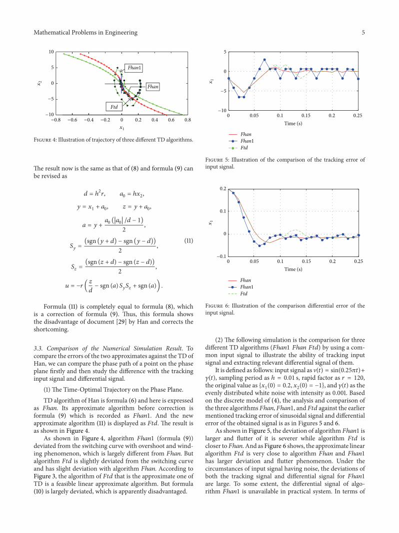
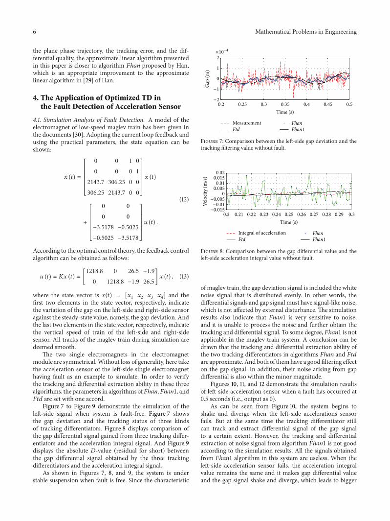
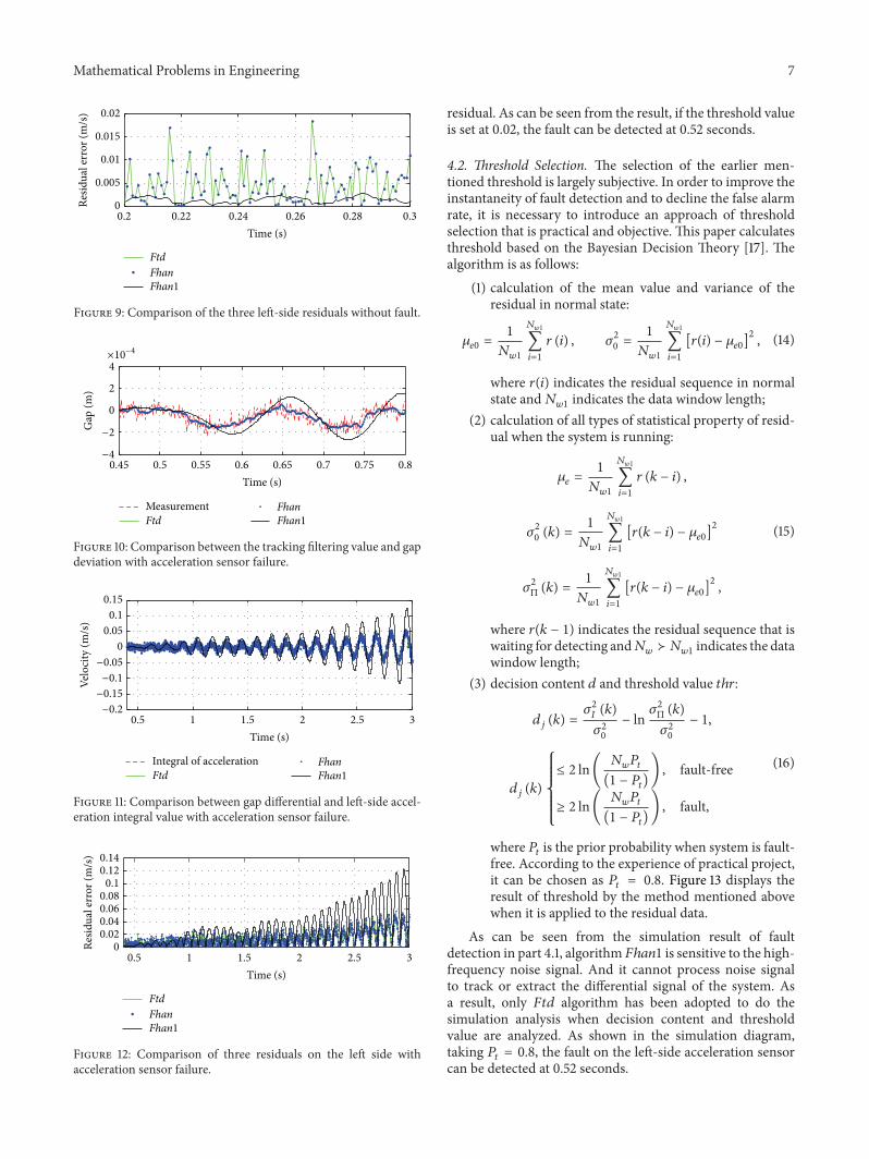
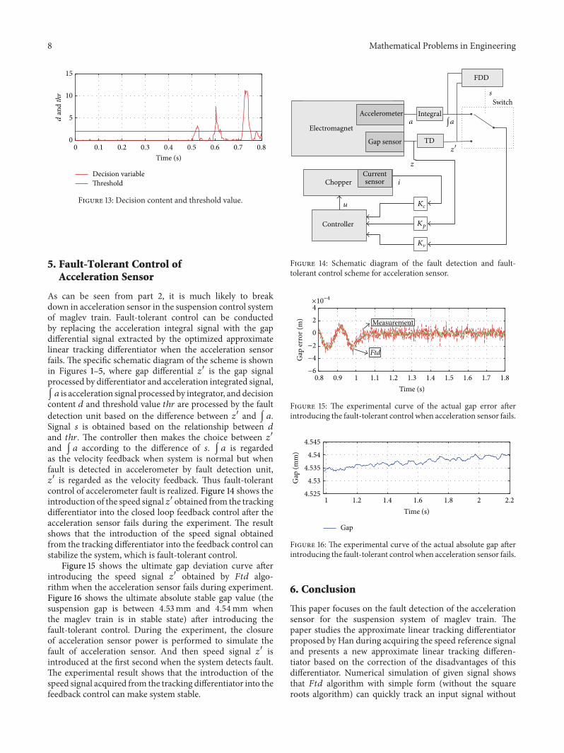