Embed Size (px)
Citation preview
Hindawi Publishing CorporationMathematical Problems in EngineeringVolume 2008, Article ID 578723, 11 pagesdoi:10.1155/2008/578723
Research ArticleExact and Numerical Solutions of Poisson Equationfor Electrostatic Potential Problems
Selcuk Yıldırım
Department of Electrical Education, Firat University, 23119 Elazig, Turkey
Correspondence should be addressed to Selcuk Yıldırım, [email protected]
Received 19 September 2007; Accepted 17 March 2008
Recommended by Mohammad Younis
Homotopy perturbation method (HPM) and boundary element method (BEM) for calculating theexact and numerical solutions of Poisson equation with appropriate boundary and initial conditionsare presented. Exact solutions of electrostatic potential problems defined by Poisson equation arefound using HPM given boundary and initial conditions. The same problems are also solved usingthe BEM. The cell integration approach is used for solving Poisson equation by BEM. The problemregion containing the charge density is subdivided into triangular elements. In addition, this paperpresents a numerical comparison with the HPM and BEM.
Copyright q 2008 Selcuk Yıldırım. This is an open access article distributed under the CreativeCommons Attribution License, which permits unrestricted use, distribution, and reproduction inany medium, provided the original work is properly cited.
1. Introduction
It is well known that there are many linear and nonlinear partial equations in variousfields of science and engineering. The solution of these equations can be obtained by manydifferent methods. In recent years, the studies of the analytical solutions for the linear ornonlinear evolution equations have captivated the attention of many authors. The numericaland seminumerical/analytic solution of linear or nonlinear, ordinary differential equationor partial differential equation has been extensively studied in the resent years. There areseveral methods have been developed and used in different problems [1–3]. The homotopyperturbation method is relatively new and useful for obtaining both analytical and numericalapproximations of linear or nonlinear differential equations [4–7]. This method yields a veryrapid convergence of the solution series. The applications of homotopy perturbation methodamong scientists received more attention recently [8–10]. In this study, we will first concentrateon analytical solution of Poisson equation, using frequently in electrical engineering, in theform of Taylor series by homotopy perturbation method [11–13].
The boundary element method is a numerical technique to solve boundary valueproblems represented by linear partial differential equations [14] and has some important
2 Mathematical Problems in Engineering
advantages. The main advantage of the BEM is that it replaces the original problem withan integral equation defined on the boundary of the solution domain. For the case of ahomogeneous partial differential equation, the BEM requires only the discretization on theboundary of the domain [15]. If the simulation domain is free from the electric charge,the governing equation is known as Laplace equation. The BEM computes an approximatesolution for the boundary integral formulation of Laplace’s equation by discretizing theproblem boundary into separate elements, each containing a number of collocation nodes.
The distribution of the electrostatic potential can be determined by solving Poissonequation, if there is charge density in problem domain. In this case, the boundary integralequation obtained from Poisson equation has a domain integral. In the BEM, several methodshad been developed for solving this integral. These methods are commonly known ascell integration approach, dual reciprocity method (DRM) and multiple reciprocity method(MRM) [16].
The electric field is related to the charge density by the divergence relationship
E = electric field,
∇E =ρ
ε0, ρ = charge density,
ε0 = permittivity,
(1.1)
and the electric field is related to the electric potential by a gradient relationship
E = −∇V. (1.2)
Therefore the potential is related to the charge density by Poisson equation:
∇ · ∇V = ∇2V =−ρε0, V = electric potential. (1.3)
2. Theory of the numerical methods
2.1. Homotopy perturbation method
Homotopy perturbation method has been suggested to solve boundary value problems in[17–19]. According to this method, a homotopy with an imbedding parameter p ∈ [0, 1]is constructed and the imbedding parameter is considered as a “small parameter”. Here,homotopy perturbation method is used to solve analytic solution of Poisson equation withgiven boundary conditions.
To illustrate this method, we consider the following nonlinear differential equation:
A(u) − f(r) = 0, r ∈ Ω, (2.1)
with boundary condition
B
(u,∂u
∂n
)= 0, r ∈ Γ, (2.2)
Selcuk Yıldırım 3
where A(u) is written as follows:
A(u) = L(u) +N(u). (2.3)
A is a general differential operator, B is a boundary operator, f(r) is a known analyticalfunction and Γ is the boundary of the domain Ω. The operator A can be generally divided intotwo parts L and N, where L is linear operator and N is nonlinear operator. Thus, (2.1) can berewritten as follows:
L(u) +N(u) − f(r) = 0. (2.4)
By the homotopy technique [20], we obtain a homotopy ν(r, p) : Ω×[0, 1]→ R satisfying
H(ν, p) = (1 − p)[L(ν) − L
(u0)]
+ p[A(ν) − f(r)] = 0, p ∈ [0, 1], r ∈ Ω, (2.5)
where p ∈ [0, 1] is an embedding parameter and u0 is an initial approximation of (2.1), whichsatisfies the boundary conditions. Clearly, from (2.5), we have
H(ν, 0) = L(ν) = L(u0)= 0,
H(ν, 1) = A(ν) = f(r) = 0,(2.6)
the changing process of p from zero to unity is just that of ν(r, p) from u0(r) to u(r). In topologythis is called deformation and L(ν) − L(u0), A(ν) − f(r) are called homotopic.
We consider ν as follows:
ν = ν0 + pν1 + p2ν2 + p3ν3 + · · · =∞∑n=0
pnνn. (2.7)
According to homotopy perturbation method, an acceptable approximation solution of(2.4) can be explained as a series of the power of p,
u = limp→1
ν = ν0 + ν1 + ν2 + ν3 + · · · =∞∑n=0
νn. (2.8)
Convergence of the series (2.8) is given in [20, 21]. Besides, the same results have beendiscussed in [22–24].
2.2. Boundary element method
Consider the Poisson equation
∇2u=b0, (2.9)
where b0 is a known function (for the electrostatic problems, according to Gauss law is b0 =−ρ/ε0).

4 Mathematical Problems in Engineering
We can develop the boundary element method for the solution of ∇2u = b0 in a two-dimensional domain Ω. We must first form an integral equation from the Poisson equation byusing a weighted integral equation and then use the Green-Gauss theorem:
∫Ω
(∇2u − b0
)w0dΩ =
∫Γ
∂u
∂nw0dΓ −
∫Ω∇u · ∇w0dΩ. (2.10)
To derive the starting equation for the boundary element method, we use the Green-Gauss theorem again on the second integral. This gives
∫Ωu(∇2w0
)dΩ −
∫Ωbw0dΩ =
∫Γu∂w0
∂ndΓ −
∫Γw0
∂u
∂ndΓ, (2.11)
and thus, the boundary integral equations are obtained for a domain Ω with boundary Γ, whereu potential, ∂u/∂n, is derivative with respect to normal of u and w0 is the known fundamental
solution to Laplace’s equation applied at point ξ(w0 = −(1/2π)�nr). r =√(ξ − x)2 + (η − y)2
(singular at the point (ξ, η) ∈ Ω).Then, using the property of the Dirac delta from (2.11),
∫Ωu(∇2w0
)dΩ = −
∫Ωuδ(ξ − x, η − y)dΩ = −u(ξ, η), (ξ, η) ∈ Ω, (2.12)
that is, the domain integral has been replaced by a point value [25].Thus, from Poisson equation the boundary integral equation is obtained on the boun-
dary:
c(ξ)u(ξ) +∫Γu∂w0
∂ndΓ +
∫Ωb0w0dΩ =
∫Γw0
∂u
∂ndΓ, (2.13)
where
c(ξ) =
⎧⎨⎩
1 in Ω,12
on Γ.(2.14)
The boundary integral equation for the internal points is
u(ξ) =∫Γw0
∂u
∂ndΓ −
∫Γu∂w0
∂ndΓ −
∫Ωb0w0dΩ. (2.15)
2.2.1. Cell integration approach
One of solution of domain integral in the BEM is cell integration approach which is the problemregion subdivided to triangular elements as done in the finite element method (Figure 1).Domain integral is solved with respect to relationship between all cells and each boundarynode by Gauss quadraturemethod.
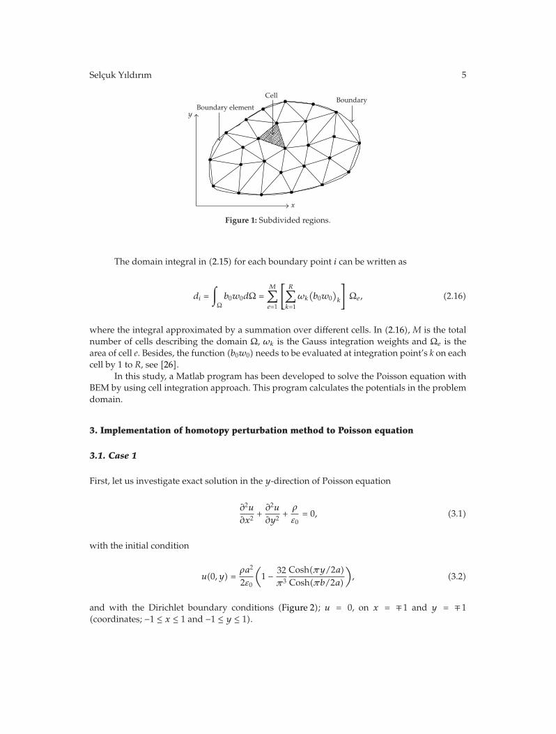
Selcuk Yıldırım 5
BoundaryCell
Boundary elementy
x
Figure 1: Subdivided regions.
The domain integral in (2.15) for each boundary point i can be written as
di =∫Ωb0w0dΩ =
M∑e=1
[R∑k=1
ωk
(b0w0
)k
]Ωe, (2.16)
where the integral approximated by a summation over different cells. In (2.16), M is the totalnumber of cells describing the domain Ω, ωk is the Gauss integration weights and Ωe is thearea of cell e. Besides, the function (b0w0) needs to be evaluated at integration point’s k on eachcell by 1 to R, see [26].
In this study, a Matlab program has been developed to solve the Poisson equation withBEM by using cell integration approach. This program calculates the potentials in the problemdomain.
3. Implementation of homotopy perturbation method to Poisson equation
3.1. Case 1
First, let us investigate exact solution in the y-direction of Poisson equation
∂2u
∂x2+∂2u
∂y2+ρ
ε0= 0, (3.1)
with the initial condition
u(0, y) =ρa2
2ε0
(1 − 32
π3
Cosh(πy/2a)Cosh(πb/2a)
), (3.2)
and with the Dirichlet boundary conditions (Figure 2); u = 0, on x = ∓ 1 and y = ∓ 1(coordinates; −1 ≤ x ≤ 1 and −1 ≤ y ≤ 1).
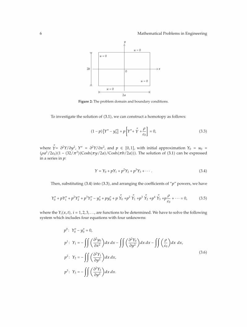
6 Mathematical Problems in Engineering
2b
2a
u = 0
u = 0
u = 0
u = 0
0
y
x
Figure 2: The problem domain and boundary conditions.
To investigate the solution of (3.1), we can construct a homotopy as follows:
(1 − p)[Y ′′ − y′′0
]+ p
[Y ′′+
′′Y +
ρ
ε0
]= 0, (3.3)
where′′Y= ∂2Y/∂y2, Y ′′ = ∂2Y/∂x2, and p ∈ [0, 1], with initial approximation Y0 = u0 =
(ρa2/2ε0)(1 − (32/π3)(Cosh(πy/2a)/Cosh(πb/2a))). The solution of (3.1) can be expressedin a series in p:
Y = Y0 + pY1 + p2Y2 + p3Y3 + · · · . (3.4)
Then, substituting (3.4) into (3.3), and arranging the coefficients of “p” powers, we have
Y ′′0 + pY ′′1 + p2Y ′′2 + p3Y ′′3 − y′′0 + py′′0 + p′′Y0 +p2
′′Y1 +p3
′′Y2 +p4
′′Y3 +p
ρ
ε0+ · · · = 0, (3.5)
where the Yi(x, t), i = 1, 2, 3, . . ., are functions to be determined. We have to solve the followingsystem which includes four equations with four unknowns:
p0 : Y ′′0 − y′′0 = 0,
p1 : Y1 = −∫∫ (
∂2y0
∂x2
)dx dx −
∫∫ (∂2Y0
∂y2
)dx dx −
∫∫ (ρ
ε0
)dx dx,
p2 : Y2 = −∫∫ (
∂2Y1
∂y2
)dx dx,
p3 : Y3 = −∫∫ (
∂2Y2
∂y2
)dx dx.
(3.6)
Selcuk Yıldırım 7
To found unknowns Y1, Y2, Y3, . . . , we must use the initial condition (3.2) for the abovesystem, then we obtain
Y0 =ρa2
2ε0
(1 − 32
π3
Cosh(πy/2a)Cosh(πb/2a)
),
Y1 =16 ρa2
π3ε0
x2
2!
(π
2a
)2 Cosh(πy/2a)Cosh(πb/2a)
− x2
2ρ
ε0,
Y2 =16 ρa2
π3ε0
x4
4!
(π
2a
)4 Cosh(πy/2a)Cosh(πb/2a)
,
Y3 =16 ρa2
π3ε0
x6
6!
(π
2a
)6 Cosh(πy/2a)Cosh(πb/2a)
,
...
(3.7)
Thus, as considering (3.4) with (3.7) and using Taylor series, we obtain the analyticalsolutions as
u =ρa2
2ε0−
16 ρa2
π3ε0
Cosh(πy/2a)Cosh(πb/2a)
[1 − 1
2!
(πx
2a
)2
+14!
(πx
2a
)4
− 16!
(πx
2a
)6
+ · · ·]− x
2
2ρ
ε0. (3.8)
Therefore, the exact solution of u(x, y) in closed form is
u(x, y) =ρa2
2ε0
(1 − x
2
a2
)−
16 ρa2
π3ε0
Cosh(πy/2a)Cosh(πb/2a)
Cosπx
2a. (3.9)
3.2. Case 2
Let us investigate exact solution in the x-direction of Poisson equation
∂2u
∂x2+∂2u
∂y2+ρ
ε0= 0, (3.10)
with the initial condition
u(x, 0) =ρb2
2ε0
(1 − 32
π3
Cosh(πx/2b)Cosh(πa/2b)
), (3.11)
and with the Dirichlet boundary conditions. To investigate the solution of (3.10), we canconstruct a homotopy as follows:
(1 − p)[ ′′Y −
′′y0
]+ p
[Y ′′+
′′Y +
ρ
ε0
]= 0. (3.12)
8 Mathematical Problems in Engineering
0 0 0 0
0
0 0 0 0
0
0.05
0.05
0.15
0.2
0.2
0.2 0.25
0.25
0.250.25
0.1
0.05
0.050.05
0.050.050.
05
0.05
0.05
0.1
0.1
0.1
0.1
0.10.1
0.1
0.15
0.15
0.15
0.15
0.15
0.150.2
0.2
0.2
10.80.60.40.20−0.2−0.4−0.6−0.8−1x-coordinate
−1
−0.8
−0.6
−0.4
−0.2
0
0.2
0.4
0.6
0.8
1
y-c
oord
inat
e
Figure 3: Equipotential lines for ρ/ε0 = 1 (using HPM, x-direction).
After that, substituting (3.4) into (3.12), and arranging the coefficients of “p” powers, wehave to solve the following system including four equations with four unknowns:
p0 : Y ′′0 − y′′0 = 0,
p1 : Y1 = −∫∫ (
∂2y0
∂x2
)dy dy −
∫∫ (∂2Y0
∂y2
)dy dy −
∫∫ (ρ
ε0
)dy dy,
p2 : Y2 = −∫∫ (
∂2Y1
∂x2
)dy dy,
p3 : Y3 = −∫∫ (
∂2Y2
∂x2
)dy dy.
(3.13)
As found unknowns Y1, Y2, Y3, . . ., we have exact solution of (3.10):
u(x, y) =ρb2
2ε0−
16 ρb2
π3ε0
Cosh(πx/2b)Cosh(πa/2b)
[1 − 1
2!
(πy
2b
)2
+14!
(πy
2b
)4
− 16!
(πy
2b
)6
+ · · ·]−y2
2ρ
ε0.
(3.14)
Therefore, the exact solution of u(x, y) in closed form is
u(x, y) =ρb2
2ε0
(1 −
y2
b2
)−
16ρb2
π3ε0
Cosh(πx/2b)Cosh(πa/2b)
Cosπy
2b. (3.15)
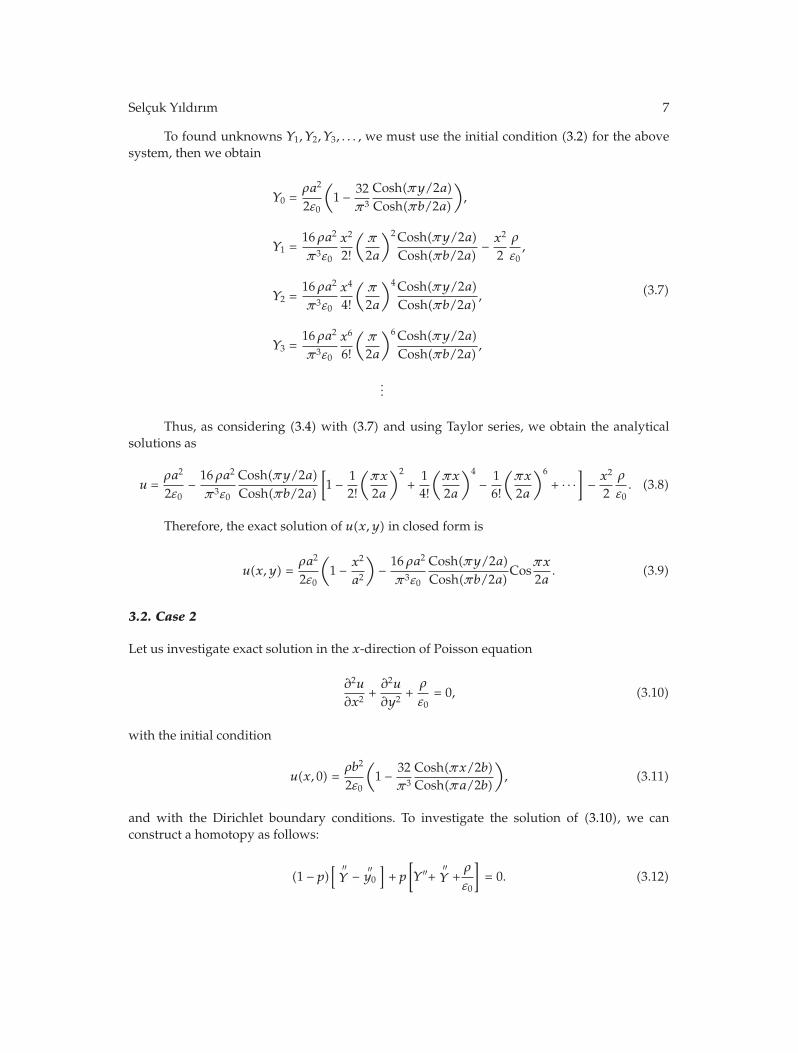
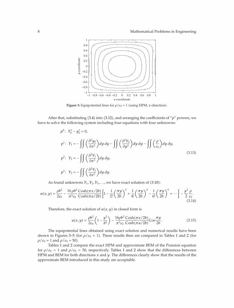
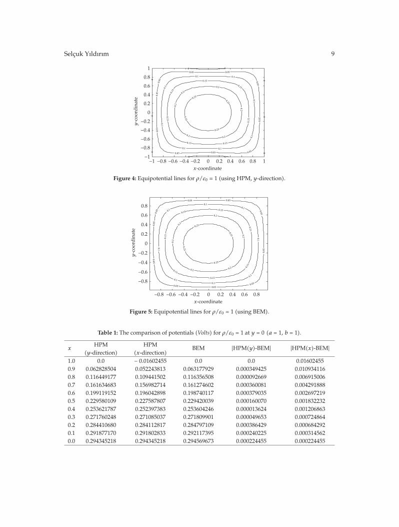
The equipotential lines obtained using exact solution and numerical results have beenshown in Figures 3–5 (for ρ/ε0 = 1). These results then are compared in Tables 1 and 2 (forρ/ε0 = 1 and ρ/ε0 = 50).
Tables 1 and 2 compare the exact HPM and approximate BEM of the Poission equationfor ρ/ε0 = 1 and ρ/ε0 = 50, respectively. Tables 1 and 2 show that the differences betweenHPM and BEM for both directions x and y. The differences clearly show that the results of theapproximate BEM introduced in this study are acceptable.
Selcuk Yıldırım 9
00
0
0 0
0 0
00
0
0.05
0.05 0.05
0.05
0.05
0.050.050.05
0.05
0.05
0.1
0.1 0.1
0.1
0.1
0.10.1
0.1
0.15
0.15
0.15
0.15
0.150.15
0.15
0.2
0.2
0.2
0.20.2
0.2
0.25
0.25
0.25
0.25
10.80.60.40.20−0.2−0.4−0.6−0.8−1x-coordinate
−1
−0.8
−0.6
−0.4
−0.2
0
0.2
0.4
0.6
0.8
1
y-c
oord
inat
e
Figure 4: Equipotential lines for ρ/ε0 = 1 (using HPM, y-direction).
0.05
0.05 0.05
0.05
0.05
0.05
0.050.05
0.05
0.05
0.1
0.10.1
0.1
0.1
0.1
0.1
0.1
0.150.15
0.15
0.15
0.15
0.15
0.15
0.2
0.2
0.2
0.20.2
0.2
0.25
0.25
0.25
0.25
0.80.60.40.20−0.2−0.4−0.6−0.8x-coordinate
−0.8
−0.6
−0.4
−0.2
0
0.2
0.4
0.6
0.8
y-c
oord
inat
e
Figure 5: Equipotential lines for ρ/ε0 = 1 (using BEM).
Table 1: The comparison of potentials (Volts) for ρ/ε0 = 1 at y = 0 (a = 1, b = 1).
xHPM HPM BEM |HPM(y)-BEM| |HPM(x)-BEM|
(y-direction) (x-direction)1.0 0.0 − 0.01602455 0.0 0.0 0.016024550.9 0.062828504 0.052243813 0.063177929 0.000349425 0.0109341160.8 0.116449177 0.109441502 0.116356508 0.000092669 0.0069150060.7 0.161634683 0.156982714 0.161274602 0.000360081 0.0042918880.6 0.199119152 0.196042898 0.198740117 0.000379035 0.0026972190.5 0.229580109 0.227587807 0.229420039 0.000160070 0.0018322320.4 0.253621787 0.252397383 0.253604246 0.000013624 0.0012068630.3 0.271760248 0.271085037 0.271809901 0.000049653 0.0007248640.2 0.284410680 0.284112817 0.284797109 0.000386429 0.0006842920.1 0.291877170 0.291802833 0.292117395 0.000240225 0.0003145620.0 0.294345218 0.294345218 0.294569673 0.000224455 0.000224455

10 Mathematical Problems in Engineering
Table 2: The comparison of potentials (Volts) for ρ/ε0 = 50 at x = 0 (a = 1, b = 1).
yHPM HPM BEM |HPM(y)-BEM| |HPM(x)-BEM|
(y-direction) (x-direction)1.0 − 0.80122754 0.0 0.0 0.80122754 0.00.9 2.612190681 3.141425217 3.158722460 0.546531779 0.0172972430.8 5.472075101 5.822458882 5.815100354 0.343025253 0.0073585280.7 7.849135743 8.081734156 8.083558316 0.234422573 0.0018241600.6 9.802144924 9.955957630 9.930100041 0.127955117 0.0258575890.5 11.37939038 11.47900548 11.46598698 0.08659660 0.013018500.4 12.61986917 12.68108935 12.67698049 0.05711132 0.004108860.3 13.55425187 13.58801241 13.60251771 0.04826584 0.014505300.2 14.20564089 14.22053401 14.22555053 0.01990964 0.005016520.1 14.59014168 14.59385852 14.62567229 0.03553061 0.031813770.0 14.71726094 14.71726094 14.72848367 0.01122273 0.01122273
4. Conclusions
In this paper, we proposed homotopy perturbation method to find exact solution in the x-and y-directions of Poisson equation with appropriate boundary and initial conditions. Thenumerical results of this electrostatic potential problem have been calculated at the sameboundary conditions by BEM. These results are compared with those of HPM in Tables 1 and2. The obtained numerical results by using BEM are in agreement with the exact solutionsobtained by HPM. This adjustment is clearly seen in Figures 3, 4, and 5. It is shown that thesemethods are acceptable and very efficient for solving electrostatic field problems with chargedensity.
References
[1] G. Adomian, “A review of the decomposition method in applied mathematics,” Journal of MathematicalAnalysis and Applications, vol. 135, no. 2, pp. 501–544, 1988.
[2] J.-H. He, “Variational iteration method—a kind of non-linear analytical technique: some examples,”International Journal of Non-Linear Mechanics, vol. 34, no. 4, pp. 699–708, 1999.
[3] S. J. Liao, Beyond Perturbation: Introduction to Homotopy Analysis Method, vol. 2 of CRC Series: ModernMechanics and Mathematics, Chapman & Hall/CRC Press, Boca Raton, Fla, USA, 2004.
[4] S. Abbasbandy, “Modified homotopy perturbation method for nonlinear equations and comparisonwith Adomian decomposition method,” Applied Mathematics and Computation, vol. 172, no. 1, pp. 431–438, 2006.
[5] J.-H. He, “The homotopy perturbation method nonlinear oscillators with discontinuities,” AppliedMathematics and Computation, vol. 151, no. 1, pp. 287–292, 2004.
[6] J.-H. He, “Some asymptotic methods for strongly nonlinear equations,” International Journal of ModernPhysics B, vol. 20, no. 10, pp. 1141–1199, 2006.
[7] T. Ozis and A. Yildirim, “A comparative study of He’s homotopy perturbation method fordetermining frequency-amplitude relation of a nonlinear oscillator with discontinuities,” InternationalJournal of Nonlinear Sciences and Numerical Simulation, vol. 8, no. 2, pp. 243–248, 2007.
[8] T. Ozis and A. Yildirim, “Traveling wave solution of Korteweg-de Vries equation using He’shomotopy perturbation method,” International Journal of Nonlinear Sciences and Numerical Simulation,vol. 8, no. 2, pp. 239–242, 2007.
[9] J.-H. He, “New interpretation of homotopy perturbation method,” International Journal of ModernPhysics B, vol. 20, no. 18, pp. 2561–2568, 2006.

Selcuk Yıldırım 11
[10] S. Abbasbandy, “Application of He’ homotopy perturbation method to functional integral equations,”Chaos, Solitons and Fractals, vol. 31, no. 5, pp. 1243–1247, 2007.
[11] L.-N. Zhang and J.-H. He, “Homotopy perturbation method for the solution of the electrostaticpotential differential equation,” Mathematical Problems in Engineering, vol. 2006, Article ID 83878, 6pages, 2006.
[12] S. T. Mohyud-Din and M. A. Noor, “Homotopy perturbation method for solving fourth-orderboundary value problems,” Mathematical Problems in Engineering, vol. 2007, Article ID 98602, 15 pages,2007.
[13] K. Al-Khaled, “Theory and computation in singular boundary value problems,” Chaos, Solitons andFractals, vol. 33, no. 2, pp. 678–684, 2007.
[14] C. A. Brebbia and S. Walker, Boundary Element Techniques in Engineering, Newnes-Butterworths,London, UK, 1980.
[15] P. K. Kythe, An Introduction to Boundary Element Method, CRC Press, Boca Raton, Fla, USA, 1995.[16] P. W. Partridge, C. A. Brebbia, and L. C. Wrobel, The Dual Reciprocity Boundary Element Method,
International Series on Computational Engineering, Computational Mechanics and Elsevier AppliedScience, Southampton, UK, 1992.
[17] M. A. Noor and S. T. Mohyud-Din, “An efficient algorithm for solving fifth-order boundary valueproblems,” Mathematical and Computer Modelling, vol. 45, no. 7-8, pp. 954–964, 2007.
[18] M. A. Noor and S. T. Mohyud-Din, “Homotopy perturbation method for solvingsixth-order boundaryvalue problems,” Computers & Mathematics with Applications. In press.
[19] M. A. Noor and S. T. Mohyud-Din, “Variational iteration method for solving higher-order nonlinearboundary value problems using He’s polynomials,” International Journal of Nonlinear Sciences andNumerical Simulation, vol. 9, no. 2, 2008.
[20] J.-H. He, “Homotopy perturbation technique,” Computer Methods in Applied Mechanics and Engineering,vol. 178, no. 3-4, pp. 257–262, 1999.
[21] J.-H. He, “A coupling method of a homotopy technique and a perturbation technique for non-linearproblems,” International Journal of Non-Linear Mechanics, vol. 35, no. 1, pp. 37–43, 2000.
[22] J.-H. He, “Homotopy perturbation method for solving boundary value problems,” Physics Letters A,vol. 350, no. 1-2, pp. 87–88, 2006.
[23] J.-H. He, “Homotopy perturbation method: a new nonlinear analytical technique,” Applied Mathemat-ics and Computation, vol. 135, no. 1, pp. 73–79, 2003.
[24] J.-H. He, “Comparison of homotopy perturbation method and homotopy analysis method,” AppliedMathematics and Computation, vol. 156, no. 2, pp. 527–539, 2004.
[25] P. Hunter and A. Pullan, “FEM/BEM notes,” Ph. D. thesis, Department of Engineering Science,University of Auckland, Auckland, New Zealand, 2001.
[26] S. Yıldırım, “The investigation of electric fields in high voltage systems using the boundary elementmethod,” Ph. D. thesis, Graduate School of Natural and Applied Science, Firat University, Elazig,Turkey, 1999.

Submit your manuscripts athttp://www.hindawi.com
Hindawi Publishing Corporationhttp://www.hindawi.com Volume 2014
MathematicsJournal of
Hindawi Publishing Corporationhttp://www.hindawi.com Volume 2014
Mathematical Problems in Engineering
Hindawi Publishing Corporationhttp://www.hindawi.com
Differential EquationsInternational Journal of
Volume 2014
Applied MathematicsJournal of
Hindawi Publishing Corporationhttp://www.hindawi.com Volume 2014
Probability and StatisticsHindawi Publishing Corporationhttp://www.hindawi.com Volume 2014
Journal of
Hindawi Publishing Corporationhttp://www.hindawi.com Volume 2014
Mathematical PhysicsAdvances in
Complex AnalysisJournal of
Hindawi Publishing Corporationhttp://www.hindawi.com Volume 2014
OptimizationJournal of
Hindawi Publishing Corporationhttp://www.hindawi.com Volume 2014
CombinatoricsHindawi Publishing Corporationhttp://www.hindawi.com Volume 2014
International Journal of
Hindawi Publishing Corporationhttp://www.hindawi.com Volume 2014
Operations ResearchAdvances in
Journal of
Hindawi Publishing Corporationhttp://www.hindawi.com Volume 2014
Function Spaces
Abstract and Applied AnalysisHindawi Publishing Corporationhttp://www.hindawi.com Volume 2014
International Journal of Mathematics and Mathematical Sciences
Hindawi Publishing Corporationhttp://www.hindawi.com Volume 2014
The Scientific World JournalHindawi Publishing Corporation http://www.hindawi.com Volume 2014
Hindawi Publishing Corporationhttp://www.hindawi.com Volume 2014
Algebra
Discrete Dynamics in Nature and Society
Hindawi Publishing Corporationhttp://www.hindawi.com Volume 2014
Hindawi Publishing Corporationhttp://www.hindawi.com Volume 2014
Decision SciencesAdvances in
Discrete MathematicsJournal of
Hindawi Publishing Corporationhttp://www.hindawi.com
Volume 2014 Hindawi Publishing Corporationhttp://www.hindawi.com Volume 2014
Stochastic AnalysisInternational Journal of


![Electrostatic Excitation of a Conducting Toroid: Exact Solution …scharstein.eng.ua.edu/toroid.pdf · so that a Fourier sine series is required in the form sinη [2coshξ0 −2cosη]3/2](https://img.dokumen.tips/doc/110x75/5f37d6496d7ebb576202132b/electrostatic-excitation-of-a-conducting-toroid-exact-solution-so-that-a-fourier.jpg)