Embed Size (px)
Citation preview

STANFORD RESEARCH INSTITUTEMenlo Park, California 94025 • U.S.A.
Semiannual Progress Report
Covering the Period 7 October 1970 to 31 March 1971
April 1971
RESEARCH AND APPLICATIONSARTIFICIAL INTELLIGENCE
By B RAPHAEL L J CHAITIN R 0 DUDAR E FIKES P E HART N J NILSSON
Prepared For
NATIONAL AERONAUTICS AND SPACE ADMINISTRATIONOFFICE OF ADVANCED RESEARCH AND TECHNOLOGYRESEARCH DIVISIONWASHINGTON, DC 20546
CONTRACT NASW-2164
SRI Project 8973
Approved By
DAVID R BROWN, Director,Information Science Laboratory
BONNAR COX, Executive DirectorInformation Science and Engineering Division
Copy No
https://ntrs.nasa.gov/search.jsp?R=19730013831 2020-05-10T03:29:59+00:00Z

ABSTRACT
This is a semiannual progress report about a program of research in
the field of Artificial Intelligence. The research areas discussed in-
clude automatic theorem proving, representations of real-world environ-
ments, problem-solving methods, the design of a programming system for
problem-solving research, techniques for general scene analysis based
upon television data, and the problems of assembling an integrated robot
system. Major accomplishments include the development of a new problem-
solving system that uses both formal logical inference and informal
heuristic methods, the development of a method of automatic learning by
generalization, and the design of the overall structure of a new complete
robot system. Eight appendices to the report contain extensive technical
details of the work described.
111

CONTENTS
ABSTRACT
LIST OF ILLUSTRATIONS
LIST OF TABLES
I INTRODUCTION
A. General
B. Background
C. The Problem
D. Report Organization
II INDEPENDENT RESEARCH STUDIES
A. Automatic Theorem Proving
B. Models of the Environment
C. Problem-Solving Studies
D. Language Development
Ill ASSEMBLING AN INTEGRATED ROBOT SYSTEM
A. The Executive
B. Intermediate-Level Actions
C. ' The Construction of Generalized Plans
IV VISION RESEARCH
A. Introduction. . .
B. Vision Programs for Intermediate-Level Actions.
C. Techniques for General Scene Analysis
V HARDWARE AND SYSTEMS SOFTWARE
A. Introduction
111
Vll
ix
1
1
2
2
3
7
7
9
17
20
23
23
25
32
41
41
41
44
49
49

B. Hardware 49
C. Diagnostic and Monitor Programs 52
D. User Support Programs 53
REFERENCES 55
Appendix A—A HEURISTICALLY GUIDED EQUALITY RULE IN ARESOLUTION THEOREM PROVER 57
(Claude R. Brice and Jan A. Derksen)
Appendix B--REASONING BY ANALOGY AS AN AID TO HEURISTIC THEOREM
PROVING 83
(Robert E. Kling)
Appendix C--STRIPS: A NEW APPROACH TO THE APPLICATION OFTHEOREM PROVING TO PROBLEM SOLVING 99
(Richard E. Fikes and Nils J. Nilsson)
Appendix D--A LANGUAGE FOR WRITING PROBLEM-SOLVING PROBLEMS , . . 137(Johns F. Rulifson, Richard J. Waldinger and
Jan A . Derksen)
Appendix E—FAILURE TESTS AND GOALS IN PLANS 151(Richard E. Fikes)
Appendix F--ISUPPOSEW--A COMPUTER PROGRAM THAT FINDS REGIONS IN
THE PLAN MODEL OF A VISUAL SCENE 171
(Kazuhiko Masuda)
Appendix G—ROBOT COMMUNICATIONS BETWEEN THE PDP-15 AND THEPDP-10 203
(B. Michael Wilber)
Appendix H—FORTRAN DISPLAY PACKAGE 225
(John Bender)
VI

ILLUSTRATIONS
Figure 1 Example Model
Figure 2 Sequence of States and Kernel States
Figure 3 Some Possible Ways of Correcting an Imperfect
Imperfectly Partitioned Picture
Figure 4 SRI Artificial Intelligence Group Computer
System
Figure B-l Venn Diagram of Relations in
Statement T, T . and Df\
Figure B-2 Relationship Between Section of ZORBA-1
and QA3
Figure C-l Flowchart for the Strips Executive
Figure C-2 Configuration of Objects and Robot
for Example Problem
Figure C-3 Solution Trace for Example Problem
Figure E-l Abstract Plan Indicating Possible Tests. . . .
Figure E-2 Plan for the Three Boxes Problem
Figure F-l Part of the Plan Model of Visual Scenes. . . .
Figure F-2 Cases for Application of Rules 4(a)
Figure F-3 Case for Application of Rule 4(b)
Figure F-4 Diagram Illustrating Rules 5 and 6
Figure F-5 Example Input Data
Figure F-6 Algorithm of CONJECT 2
Figure F-7 Explanatory Diagram for CONJECT 2
Figure F-8 Algorithm of PROCESSK
Figure F-9 Functions for Judging the Relationship
Between A Line and CDLNs
13
37
47
50
89
95
118
119
123
157
159
176
178
179
179
181
186
187
189
190
VII

Figure F-10
Figure F-ll
Figure F-12
Figure F-13
Figure F-14
Figure F-15
Figure F-16
Figure F-17
Figure F-18
Figure F-19
Diagram Illustrating the Necessity of
Checking Whether CDLN Crosses any VIEWLINE
Explanatory Diagram for Function FOOP. . .
Algorithm of FOOP
Data 1 Results
Data 2 Results
Data 3 Results
Data 4 Results
Data 5 Results
Explanatory Diagram for Closing Regions. .
Diagram for Questionable Conjecture. . . .
191
192
193
195
196
197
198
199
200
201
Vlll

TABLES
Table 1 Primitive Predicates for the Robot's
World Model 11
Table 2 Subroutine GOTOADJROOM(ROOM1,DOOR,ROOM2) 28
Table 3 Intermediate Level Actions. Routines Marked by
Asterisks are Viewed as Primitive Routines 31
Table D-l Problem Areas 141
Table D-2 Some Language Features 143
Table D-3 A Sample Expression 146
Table D-4 Expression Properties 146
Table D-5 Some Pattern Matcher Features 147
Table F-l Example Input Data 182
Table F-2 Internal Format 183
Table G-l Formats of the Messages 223
IX

I INTRODUCTION
A. General
This is a report of progress during the past six months in a program
of research into techniques and applications of the field of Artificial
Intelligence. This field deals with the development of automatic systems,
usually including general-purpose digital computers, that are able to
carry out tasks normally considered to require human intelligence. Such
systems would be capable of sensing the physical environment, solving
problems, conceiving and executing plans, and improving their behavior
with experience. Success in this research will lead to machines that
could replace men in a variety of dangerous jobs or hostile environments,
and therefore would have wide applicability for Government and industrial
use .
This project began in October 1970 as a direct continuation of work
performed and reported under previous contracts.1 Some of the work
reported here has been partially supported by other, concurrent SRI proj-
ects whose goals are closely related to the general Artificial Intelli-
gence problem. Such joint support is acknowledged below wherever relevant
During the past six months we have written several Technical Notes,
consolidating some of the results obtained both during the present proj-
ect and toward the end of the previous project. The contents of these
notes are summarized in the following sections of this report, and the
complete notes are attached as appendices .
*References are listed at the end of this report

The balance of this section summarizes our general orientation,
activities, and major results thus far in this project. Subsequent
sections and appendices contain additional technical details.
B. Background
The basic goal of our work is to develop general techniques for
achieving artificial intelligence. To this end, we are pursuing funda-
mental studies in several areas: problem solving, perception, automated
mathematics, and learning. However, we find it productive to choose as
a goal the creation of a single integrated system, and thus bring to a
common focus the activities in these separate studies. Such a specific
goal helps us define interesting research problems and measure progress
towards their solutions.
Our research method has involved studies aimed at both short-term
and long-term results. The short-term studies usually consist of first
defining an "intelligent" task that is slightly beyond present capabilities
for the system to perform, and then attempting to develop a specific
solution for that task. Long-term studies are concerned with developing
more general methods for achieving future intelligent systems. We be-
lieve that pursuing these two kinds of studies in parallel, and using
short-term task domains as test beds for proposed long-term techniques,
has been (and will continue to be) a fruitful research strategy.
C . The Problem
Our system consists of a mobile robot vehicle controlled by radio
from a large digital computer. The principal goal is to develop soft-
ware for the computer that, when used in conjunction with the hardware
of the vehicle, will produce a system capable of intelligent behavior.

Before we changed computers (at the end of 1969), our robot system
had achieved a primitive level of capabilities: It could analyze a
simple scene in a restricted laboratory environment; plan solutions to
certain problems, provided that exactly the correct data were appropriately
encoded; and carry out its plans, provided nothing went wrong during
execution. Therefore, when we began planning a new software system for
controlling the robot from a new computer, we set more difficult short-
term goals: The system is to be able to operate in a larger environment,
consisting of several rooms, corridors, and doorways; its planning ability
must be able to select relevant data from a large store of facts about
the world and the robot's capabilities; and it must be able to recover
gracefully from certain unexpected failures or accumulated errors.
We have not yet accomplished these goals. However, we have essen-
tially completed the design and partial implementation of a system that
we believe can exhibit such performance. This system differs from our
previous robot system in several basic ways . We expect to demonstrate
the new system before the end of the next six-month period.
D. Report Organization
The remainder of this progress report consists of four major sections
and eight appendices, describing our current robot system and associated
longer-term studies . We now present brief overviews of the contents of
those sections.
Every integrated "artificially intelligent" system must contain
several component elements. Some of these elements may define signifi-
cant long-term research fields, as well as requiring short-term formula-
tion as part of a current system. Section II describes our recent progress
in several of these areas: logic, modeling, planning, and implementation
language. Our logical inference research is still based upon the QA3.5

program for proving theorems in first-order predicate calculus. However,
the basic inference rule (viz., resolution) has been considerably aug-
mented by a variety of devices, e.g., predicate evaluation, heuristic
equality substitution, and parametric terms, that enable close coupling
between the general inference program and a particular problem domain.
How to model the real world is a basic problem in many AI systems.
Our present approach is simpler than the dual geometric and symbolic
models that we used in previous years, and is highly related to the logic
system.
Part C of Section II describes our work on problem-solving systems.
Our previous use of the logic system as the entire problem solver has
been discarded in favor of a more efficient scheme that uses logical
inference as a subroutine within a GPS-like2 framework.
Finally, Section II-D reports on the status of a long-term effort
to develop a new implementation language, QA4, that will simplify the
programming of future problem-solving and logic systems.
Section III is devoted to the problems, and potential benefits, of
assembling the components discussed above into a complete integrated
system. First, we consider the nature of an executive program that can
carry out plans generated by a problem solver like STRIPS. Second, we
examine a proposed internal structure of the subroutines—the "intermediate
Level Actions"—that are called upon by the executive in order to ac-
complish things in the real world. This structure, based upon a Markov
algorithm formalization, provides a conceptually easy way to specify
methods for communication between subroutines and recovery from errors.
Finally, the largest part of Section III describes a proposal for
"bootstrap learning" by constructing and storing generalized plans. This
promising technique for learning depends upon several of the previously
discussed features of the overall robot system.

Section IV describes recent work in vision research. Short-term
vision work has consisted of developing particular program packages,
compatible with the rest of the system, for gathering visual data about
an environment containing corridors and doorways. Longer-term studies
of color and stereo vision have also been initiated.
Finally, Section V discusses _the bottom-level software and hardware
that make the rest of the research possible. This consists of the robot
vehicle and its recent modifications, the PDP-10/PDP-15 computer systems,
and the software that enables LISP and FORTRAN programs on the PDP-10 to
control the vehicle by radio link from the PDP-15.

II INDEPENDENT RESEARCH STUDIES
A . Automatic Theorem Proving
QA3.5 is a question-answering system containing a resolution-based
theorem-proving program for first-order predicate calculus, and various
features for indexing axioms, extracting answers from proofs, and so on.3
During the past few months, we have completed the implementation of an
efficient version of QA3.5 on our PDP-10 computer, and added a variety
of features that make QA3.5 usable as the logic component of a larger
problem-solving system. In addition to a general clean-up of QA3 andI
its interface to other routines, we have made the following developments
in the general area of theorem proving (all aimed at extending resolution
to improve the effectiveness of automatic procedures):
Equality—A method was developed for using efficient tree-search
heuristics for guiding the use of the "paramodulation" rule of inference
for first-order logic with equality. This work is described in detail
in Appendix A, and the method has been implemented and is available for
experimentation.
Analogy—A study of reasoning by analogy has used QA3.5 proofs as
a subject domain, and has concluded that automatic theorem proving can
be aided by making appropriate use of analogies to similar proofs. This
work is detailed in Appendix B.
Evaluation—For some time a "predicate evaluation" feature has been
present in QA3.5, although this important innovation has not been ade-
quately documented. The basic idea is that it is sometimes more efficient
to use a special program to test the truth of a simple logical assertion
than to deduce its truth from axioms. (For example, this technique

would permit the inclusion of arithmetic relations such as "3 > 2" in
our axioms without axiomatizing arithmetic.) Such predicate-evaluation
functions, if appropriately used, could eliminate the need for large
(perhaps infinite) sets of axioms. QA3.5 contains provisions for in-
serting a broad class of predicate evaluation functions.
Parameters—Expressions of first-order logic in clause form, the
standard form for all resolution-based theorem provers including QA3.5,
contain two classes of individual symbols. constants, each of which has
a unique identity (unless the equality relation between two of them can
be proven), and variables, which are assumed to be universally quantified.
We have discovered that a third class of individuals, parameters, would
be extremely useful in problem-solving work and may have much wider
significance in logic. The use of parameters in a mechanism for making
an axiom set into a scheme of alternative possible axiom sets. A param-
eter is an unspecified constant. It may take on any—but only one—value
during a proof (subject to certain limitations discussed below). For
example, suppose we wish to use QA3.5 to determine a convenient initial
placement for the robot before carrying out some task. We would like to
assert that, in that initial configuration, the robot is someplace; and
then let the particular place be chosen by the normal unification pro-
cedure of the theorem prover as it considers other relevant facts. How-
ever, if we encode, "The robot is someplace," by the existential assertion,
(3place)AT(Robot,place), i.e., "There exists a place where the robot is
at," then the Skolemization process chooses a new constant to name the
place and give us the clause AT(Robot,a), where a_ cannot be identified
as any particular place that we know anything about (unless we intro-
duce many more axioms and equality). On the other hand, if we try
AT(Robot,v) where y_ is a universally quantified variable, v ranges over
all the relevant constants, but we can also prove all kinds of silly
false results (because we have asserted that the robot is everywhere at
8

at once). The solution is to use AT(Robot,p), where the parameter p is
a new kind of individual that sometimes behaves like a constant and
sometimes like a variable, giving just the appropriate results. We be-
lieve we have identified the appropriate behavior of parameters, and they
are now available within QA3.5.
The basic property of any parameter is that it represents precisely
a single element of a given domain. This property implies that parameter
names (and, therefore, their interpretations) are global to the entire
set of clauses involved in a QA3.5 proof (as opposed to variables, whose
names are local to a single clause) . This further requires^ that any
parameter appearing in a proof tree have but one interpretation in that
tree.
The allowed instantiations of a parameter are restricted in accordance
with the above basic property. Bindings can be formed between a param-
eter and another parameter, or to a non-Skolemized (possibly parameterized)
ground term only. It is illegal to bind a parameter to a variable, or
a function of variables (i.e., a nonground term), as this allows a single
parameter to represent a whole class of interpretations. Also, a param-
eter may not be instantiated by a term containing Skolem functions,
since such terms represent new individuals, while parameters are intended
to represent previously known (although perhaps not yet specified)
individuals.
B. Models of the Environment
1. The Robot's World Model
As a result of our experience with the previous robot system
and our desire to expand the robot's experimental environment to include
several rooms with their connecting hallways, we have adopted new con-
ventions for representing the robot's model of the world. In particular,

whereas the previous system had the burden of maintaining two separate
world models (i.e., a map-like grid model and an axiom model), the new
system uses a single model for all its operations (an axiom model); also,
in the new system conventions have been established for representing
doors, wall faces, rooms, objects, and the robot's status.
The model in the new system is a collection of predicate calcu-
lus statements stored as prenexed clauses in an indexed data structure.
The storage format allows the model to be used without modification as
the axiom set for STRIPS' planning operations (see Appendix C) and for
QAS.S's theorem-proving activities.
Although the system allows any predicate calculus statement to
be included in the model, most of the model will consist of unit clauses
(i.e., consisting of a single literal) as shown in Table 1. Nonunit
clauses typically occur in the model to represent disjunctions (e.g.,
box2 is either in room K2 or room K4) and to state general properties of
the world (e.g., for all locations loci and Ioc2 and for all objects
obi, if obi is at location loci and loci is not the same location as
Ioc2, then obi is not at location Ioc2) .
We have defined for the model the following five classes of
entities: doors, wall faces, rooms, objects, and the robot. For each
of these classes we have defined a set of primitive predicates which
are to be used to describe these entities in the model. Table 1 lists
these primitive predicates and indicates how they will appear in the
model. All distances and locations are given in feet and all angles
are given in degrees. These quantities are measured with respect to a
rectangular coordinate system oriented so that all wall faces are parallel
to one of the X-Y axes. The NAME predicate associated with each entity
allows a person to use names natural to him (e.g., halldoor, leftface,
K2090, etc.) rather than the less-intuitive system-generated names (e.g.,
dl, f203, r4450, etc.) .
10

Table 1
PRIMITIVE PREDICATES FOR THE ROBOT'S WORLD MODEL
Primitive
Predicate
FACES
type
name
f aceloc
grid
boundsroom
DOORS
type
name
doorlocs
joinsfaces
joinsrooms
doorstatus
ROOMS
typename
grid
OBJECTS
type
name
atinroom
shape
radius
ROBOT
typenameatthetatiltpanwhiskersirisoverriderangetvmodefocus
Literal Form
type( f ace"f ace")name(face name)faceloc(face number)grid(face grid)boundsroom( f ace room direction)
type( door"door")narae(door name)door locs( door number number)joinsfaces(door face face)joinsrooms(door room room)doorstatus(door status)
type( room" room")nameCroom name)grid(room grid)
t y pe( ob iect" object")nameCobject name)at(object number numberinroom( object room)shapeCobject shape)radius(object number)
type("robot""robot")name( " robot" name)at("robot" number number)t he ta(" robot "number)t i 1 t (" robot " number )pan(" robot "number)whisker s(" robot" integer)iris(" robot" integer)override( "robot" integer)range(" robot" number)tvmode(" robot" integer)f ocus( " robot" number)
Example Literal
typeCfl face)nameCfl leftface)facelocCfl 6.1)gndCfl gl)
boundsroom(f 1 rl east)
typeCdl door)name(dl halldoor)
doorlocs(dl 3.1 6.2)
joinsfaces(dl fl f2)
joinsrooms(dl rl r2)
doorstatus(dl "open")
type(rl room)
nameCrl K29090)
gridCrl gl)
typeCol object)
name(ol boxl)
at(ol 3 1 5 2 )
inroom(ol rl)shape(ol wedge)
radius(ol 3 1)
type( robot robot)name( robot shakey)
at(robot 4.1 7.2)
theta( robot 90.1)tilt(robot 15.2)
pan( robot 45 3)
whiskers( robot 5)
iris(robot 1)
overnde( robot 0)
range( robot 30.4)
tvmode( robot 0)
focus(robot 30.7)
11

Figure 1 shows a sample environment and a portion of the cor-
responding world model . Rooms are defined as any rectangular area, and
therefore the hallway on the left is modeled as a room. There is associ-
ated with each room a grid structure that indicates which portions of
the room's floor area have not yet been explored by the robot. During
route planning the grid is employed to help determine if a proposed path
is known blocked, known clear, or unknown.
Four wall faces are modeled in Figure 1. The FACELOC model
entry for each face indicates the face's location on either the X or Y
coordinate depending on the face's orientation. There is associated
with each face a grid structure to indicate which portions of the wall
face have not yet been explored by the robot. This grid is used in
searching wall faces for doors and signs.
Two doors are modeled in Figure 1. The DOORLOC model entry
for each door indicates the locations of the door's boundaries on either
the X or Y coordinate, depending on the orientation of the wall in which
the door lies. Any opening between adjoining rooms is modeled as a door,
so that the complete model of the environment diagrammed in Figure 1
would have a door connecting rooms Rl and R3. This door coincides with
the south face of room R3 and will always have the status "open."
The RADIUS and AT model entries for the object modeled in
Figure 1 define a circle circumscribing the object. These entries simplify
the route-planning routines by allowing each object to be considered
circular in shape. Our current set of primitive predicates for describing
objects is purposely incomplete; we will add new predicates to the set
as the need for them arises in our experiments.
We do not wish to restrict the model to only statements con-
taining primitive predicates. The motivation for defining such a predicate
class is to restrict the domain of model entries that the robot action
12

0)00
-n8 " •»_ E< S » S •§
Hill
oci inCM
_ S o ~8 •? ">_ E
& E 82: S »
LUOO5
a.
III& s &
£
8(N
•2 " «N "> 2CM r. " 2
£ - X « -S— o» O ^ J:
Mill*- C *_ 01 •£]
in _CN n
tr
& ?-8 ° 2.o "5 g o 2O a | «DC & c S •£
inT CM _ (N _O •" N >- C
IP ' -C IS r! r- •• o* » *g •; 8? s s
c^i,| „ * ; ? » § s j» ° : ; o^^S ^ - - S c S S g g o S O o 5 ^ E 3 - 2s-? gMll|i 3115111
13

routines have responsibility for updating. That is, it is clear that
the action routine that moves the robot must update the robot's location
in the model, but what else should it have to update9 The model may
contain many other entries whose validity depends on the robot's previous
location (e.g., a statement indicating that the robot is next to some
object), and the system must be able to determine that these statements
may no longer be valid after the robot's location has changed.
We have responded to this problem by assigning to the action
routines (discussed in Section IV-B) the responsibility for updating
only those model statements which are unit clauses and contain a primitive
predicate. All other statements in the model will have associated with
them the primitive predicate unit clauses on which their validity depends.
When such a nonprimitive statement is fetched from the model, a test
will be made to determine whether each of the primitive statements on
which it depends is still in the model; if not, then the nonprimitive
statement is considered invalid and is deleted from the model. This
scheme, which is also discussed in Section 2 of Appendix C, ensures that
new predicates can be easily added to the system and that existing action
routines produce valid models when they are executed.
2 . Model-Manipulating Functions
We have designed and programmed a set of LISP functions for
interacting with the world model. These functions are used both by the
experimenter (as he defines and interrogates the model) and by other
routines in the system to modify the model. To the experimenter at a
teletype, these functions are accessible as a set of commands. A brief
description of these commands follows.
ASSERT—This is the basic command for entering new axioms into
the model . The user follows the word ASSERT by either CUR or ALL to
14

indicate whether the entries are to be for the current model or are to
be considered part of all models. The system then prompts the user for
predicate calculus statements to be typed in using the QA3 .5 expression
input language. After each statement is entered, the system responds
with "OK" and requests the next statement. To exit the ASSERT mode the
. II t !tuser types I.
FETCH—This is the basic command for model queries. The user
follows the word FETCH by an atom form, and the system types out a list
of all unit clauses in the model that match the form. Each term in an
atom form is either a constant or a dollar sign. The dollar sign indi-
cates an "l don't care" term and will match anything. The last term of
an atom form can also be the characters "$*" to indicate an aribtrary
number of "l don't care" terms. For example, the atom form "(AT ROBOT
$*)" will fetch the location of the robot, and the atom form "(INROOM
$ Rl)" will fetch a list of model entries indicating each of the objects
in room Rl.
DELETE—This is the basic command for removing statements from
the model. The user follows the word DELETE by an atom form, and the
system deletes all unit clauses in the model that match the form. Atom
forms have the same syntax and semantics for the DELETE command as de-
scribed above for the FETCH command.
REPLACE—This is a hybrid command combining the operations of
DELETE and ASSERT. The user follows the word REPLACE by an atom form
and by a predicate calculus statement. The system first deletes all
unit clauses in the model matching the atom form and then enters the
statement into the model. This command is useful for operations such as
changing the robot's position in the model, indicating in the model that
a previously closed door is now open, and so forth.
15

3. Long-Term Modeling Studies
We have been investigating some different ways of representing
the robot's model of the world, for possible use in future system imple-
mentations. In particular, we will need to represent a large store of
knowledge of the world, hopefully including many objects, actions the
robot can take, and general principles about the world in which it re-
.sides. Until now we have only used small domains for specific problems
and have not entirely faced the problem of a lot of information in one
model .
The main concentration so far has been on comparing semantic
nets with the first-order predicate calculus representations now used .
Preliminary study seems to indicate that either can be used to make a
reasonable model for the robot. One major concern is that the system
have the ability to make inferences from the model—so the robot can
solve the problems posed to it. So far, we have not found any inference
mechanism for semantic nets that has the formal completeness of the
resolution-based theorem prover, QA3.5, that we now use. The net struc-
ture does, however, have the advantage of directing one's attention to
pertinent information to be used in the deduction. This is of particular
importance when the amount of information in the model is large in com-
parison with the amount needed to solve a specific problem.
A possible next step is to see if we can develop an inference
scheme for semantic nets which has some of the formal completeness
properties of logic. Another approach is to try to incorporate semantic
information into QA3.5 to guide the resolution toward the axioms perti-
nent to the current problem. Because we already have a working theorem
prover, and are getting some experience in resolution strategies, the
latter approach seems the one to pursue.
16

Another method of representation that has been used recently
entails encoding information in procedures rather than data structures .
During the next six months we plan to explore this alternative, particu-
larly with respect to using the QA4 language (see Section II-D) .
C. Problem-Solving Studies
A problem-solving process generally consists of two parts: planning
a solution, and executing the plan. Most previous work in heuristic
problem solving has really been concerned with the planning aspects,
since interesting problems of execution do not arise until a complete
robot system has been created. We shall delay discussion of our work on
the execution phase of problem solving until Section III of this report.
The need for a new planning program for our robot system followed
from our decisions, discussed above, to enlarge the robot's environment
(by adding rooms and hallways), and to model the world by predicate-
calculus formulas. In the new experimental environment a world model
will contain 100 or more formulas. The complexity of these models raised
certain difficulties with previously developed problem-solving systems,
and led to the design of a new problem-solving system.
The first difficulty was that our world models are too large for
any problem solver to create a complete new world model at each step in
its search. That is, when a problem solver considers some action taken
in the world, it creates a new model to indicate the state of the world
after the action. Typically, this new model is formed by copying the
old model and then making the changes implied by the action in the copy.
For our models this process would be extremely costly in both memory
space and computing time. Our response to this problem was to establish
conventions for representing a model as a set of changes from the initial
model given to the problem solver. That is, each model created during
17

the problem-solving process is represented by two lists: one of formulas
that exist in that model but do not exist in the initial model, and the
other of formulas that exist in the initial model but do not exist in the
new model. Since most formulas in a model are not changed by an action,
the two lists representing each new model contain only a small number of
formulas (usually less than about ten) and can be managed efficiently.
The second difficulty was that for large models, the use of axioms
to represent the effects of action routines, our previous planning method,
becomes extremely clumsy. That is, in our previous automaton system each
model change produced by an action was described by an axiom. Unfortu-
nately, it was also necessary to include axioms describing all those
portions of the model that were not changed by an action. (This latter
set of axioms allowed the system to produce those portions of the new
model which were unchanged from the old model when an action was applied.)
The problems with this scheme are basically twofold: First, a large
number of axioms need to be written by a person in order to describe an
action to the system; and secondly, when the problem solver applies an
action to a model it must perform a deductive step using one of these
axioms to produce each portion of the new model. Large world models
amplify these problems to the extent that the problem solver becomes
completely impotent. Reference 4 discusses these problems more fully.
We have responded to this second difficulty by removing the descrip-
tions of actions from the predicate calculus . We provide a form for
describing actions that requires only that the person indicate the changes
produced by the action. The assumption is made that all portions of the
model not mentioned in an action description are not changed by the
action. This assumption enables concise action descriptions to be written
with little effort. Our new problem-solving program, which we call STRIPS
(STanford Research Institute Problem Solver), contains an action-application
18

routine, which takes as input a world model and an action description,
and produces as output the model that would be produced by applying the
action to the input model. This routine uses the "change list" world-
model representation discussed above and is quite efficient, even with
large models.
The third difficulty we have responded to in our new system is that
of providing the problem solver with powerful heuristics for guiding its
search for a plan. In our previous system, all the search was carried
out by the theorem prover, QA3.5. Although the search heuristics in
QA3.5 may be adequate for proving theorems, they are unacceptably weak
when used to conduct the search for a plan in a space of world models.
Again, this difficulty is accentuated by the large models we are now
using. We have responded to this difficulty by designing STRIPS so that
standard graph-searching techniques can be applied to its search for a
solution. We may consider STRIPS to be searching in a space of world
models for a path from the initial model to a model in which a given goal
predicate is satisfied. During its search it uses the action-application
routine discussed above to create new models, and it uses the theorem
prover, QA3.5, to ask questions of any given model (e.g., Is the goal
true in this model'') . Hence, it can employ powerful heuristic-search
techniques to determine which action application to consider next, and
it can use QA3.5's powerful deductive techniques to determine properties
of individual world models .
The primary search strategy employed by STRIPS is means-ends analysis.
This strategy, borrowed from GPS,2 uses the following basic technique-
Given a world model and a goal, compare the two to determine a difference
between them, select an action that is relevant to reducing the difference,
establish a new subgoal of achieving a world model to which the relevant
action can be applied, and repeat the process to achieve the new subgoal.
19

This strategy provides STRIPS with a strong sense of direction toward a
goal and has produced very encouraging results with the problems we have
given to the program. (STRIPS is described more fully in Appendix C.)
D. Language Development
During the past six months this project has participated in the
support of the design and implementation of a new programming language,
QA4. (QA4 development is primarily supported by SRI Project 8721 under
Contract NASW-2086 with NASA.) QA4 contains a novel combination of
features that promise to make it more useful for programming theorem-
proving and problem-solving systems than any existing language. Appendix
D contains a general description of QA4.
The QA4 programming language has reached a first major milestone in
its development. Micro-QA4 is implemented. This restricted version of
the full QA4 language lacks only the more advanced control statements
and the complete pattern matcher. It includes the following debugged
program packages:
• Input-Output—A parsing system that converts the mathematical
style infix notation of the QA4 language to internal format.
e Expression Storage—A set of programs that:
(1) Store QA4 expressions in a discrimination net and
recognize equivalence of sets and expressions with
bound variables.
(2) Store and retrieve properties of expressions with
respect to QA4 "contexts," automatically handling
process-variable bindings and backtracking.
e QA4 Evaluator—A set of programs that:
20

(1) Evaluate all the QA4 primitive functions (e.g.,
PLUS and UNION).
(2) Execute QA4 statements (e.g., IF and GO).
(3) Work in small nonrecursive steps so that time can
be shared between parallel processes .
Features such as backtracking, process-control structures, set operations,
and tuple pattern matching make Micro-QA4 suitable for experimenting and
testing designs for future heuristic programs.
The immediate plans are to finish the pattern matcher and complete
the implementation of the control and strategy statements. The resulting
initial version of the full QA4 language will then be used for the con-
struction of theorem provers and automatic program writers. Throughout
the implementation, however, we have consistently used general data
structures and clear program design instead of the specific structures
and tight code dictated by space and time considerations. Thus, as we
use the language, we expect to enter an iterative cycle of modification
and extension. As we gather statistics we can properly optimize, and
as we discover language deficiencies we can extend the semantics.
21

Ill ASSEMBLING AN INTEGRATED ROBOT SYSTEM
A. The Executive
One of the difficulties in devising a robot system is that of pro-
viding feedback during the execution of plans. That is, since a plan
produced by STRIPS must be executed in the real world by a mechanical
device (as opposed to being carried out in a mathematical space or by
a simulator), consideration must be given to the possibility that opera-
tions in the plan may not accomplish what they were intended to, that
data obtained from sensory devices may be inaccurate, and that mechanical
tolerances may introduce errors as the plan is executed. Hence, we wish
STRIPS to provide information in a plan that will allow the executor to
determine whether each of the plan's actions is achieving the desired
result in the real world. The executor can then use this information
to recognize failures as they occur during plan execution, and can take
appropriate steps (e.g., initiate replanning) to put the system back on
a course toward the goal.
Appendix D describes algorithms for including the needed information
in STRIPS plans and for using that information during plan execution.
These algorithms produce and use a plan containing steps of the follow-
ing form:
Bi:BEGINFAILTEST<predicate-calculus formula)FOR Bjl,Bj2, ...,Bjn;
FAILTEST^predicate-calculus formula)FOR Bkl,Bk2, ...,Bkm;
IF(preconditions for action ^THEN DO action.
ELSE GOAL (relevant results of action.,)END;
23

The predicate-calculus formulas in the FAILTEST statements indicate what
STRIPS expects to be true in the world model at this point in the plan.
If one of these formulas is not true, then the executor deletes those
subsequent portions of the plan having the labels, Bxy, listed in the
right side of the FAILTEST statement; that is, STRIPS determines that
the portions of the plan being deleted cannot produce the desired re-
sults unless the formula in the FAILTEST statement is true, and there-
fore they should not be executed. The IF statement in the plan tests
to see whether the next action in the plan (action ) is applicable to
the model. In the case where it is, then the action is executed; in
the case where it is not, a replanning effort is initiated with the goal
being the model changes that action was expected to make. If a replan-
ning effort succeeds, then the new plan takes the place of the IF state-
ment in the old plan and execution proceeds as before. These plan for-
mation and execution schemes are designed to provide continual checking
on the progress of plan execution and to allow a productive interaction
between the planning and execution sections of the system.
A comment is in order on the status of this work. The world-model
maintenance routines and the STRIPS problem solver exist as running
programs. The mechanisms for creating and executing the FAILTEST and
IF statements in plans have been specified but have not yet been coded.
We have successfully run STRIPS with several example problems and are
engaged in experimenting with various search heuristics for it. We
have not yet had the opportunity to put the entire system together and
input a problem, have STRIPS produce a plan, and then have an executor
carry out the plan. The primary missing link presently is a set of
intermediate-level action routines (described below) for the robot.
These should be completed shortly, and we expect to be able to exercise
the entire system in the next few months.
24

B. Intermediate-Level Actions
1. Introduction
A planning program such as STRIPS assumes the existence of
certain action routines that enable the robot to interact with the world.
Thus far in this report we have assumed the availability of some such
set of routines, with their preconditions and effects assumed to be for-
malized and known to the problem solver. Now we face the task of actually
creating an appropriate set of routines.
As with most programming tasks, the problem of programming
robot actions is simplified when it is done in terms of'well-defined
subroutines. At the lowest level it is natural to define routines that
have a direct correspondence with low-level robot actions—routines for
rolling, turning, panning, taking a range reading, taking a television
picture, and so forth. However, these routines are too primitive for
high-level problem solving. Here it is desirable to assume the existence
of programs that can carry out tasks such as going to a specified place
or pushing an object from one place to another. These intermediate-
level actions (ILAs) may possess some limited problem-solving capacity,
such as the ability to plan routes and recover from certain errors, but
the ILAs are basically specialized subroutines. None of these routines
has as yet been written. However, considerable thought has been devoted
to their design, and this section describes our plans for a set of ILAs
that are suitable for use with the STRIPS problem-solving system. (Low-
level actions, the robot's elementary hardware capabilities, are described
in Section V of this report.)
Perhaps the most difficult problem that confronts the designer
of ILAs is the problem of detecting and recovering from errors. Some-
times errors are detected automatically, as when an interrupt from a
touch sensor indicates the presence of an unexpected obstacle. Other
25

times it is necessary to make explicit checks, such as checking to be
sure that a door is open before moving through it. When an error is
detected, the problem of recovery arises. This problem can be very
difficult, and is one aspect that distinguishes work in robotry from
other work in artificial intelligence.
It is natural to think of an intermediate-level action as a
composition of somewhat lower-level actions, which in turn are composi-
tions of lower-level actions. While this hierarchical organization
possesses many advantages (and is in fact the organization that we use),
it is not ideally suited for error recovery. Errors are made most fre-
quently at low levels by routines that are too primitive to cope with
them. An error message may have to be passed up through several levels
of routines before reaching one possessing sufficient knowledge of both
the world and the goal to take corrective action. If any routine can
fail in several ways, this presents the highest-level routine with a
bewildering variety of error messages to analyze, and requires explicit
coding for a large number of contingencies.
To circumvent this problem, we have chosen to have the sub-
routines communicate through the model. With a few special exceptions,
neither answers nor'error messages are explicitly returned by subroutines.
Instead, each routine uses the information it gains to update the model.
It is the responsibility of the calling routine to check the model to be
sure that conditions are correct before taking the next step in a sequence
of actions. Detection of an error causes returns through the sequence
of calling programs until the routine that is prepared to handle that
kind of error is reached. In the following sections we describe in more
detail the formal mechanism by which this is done.
26

2. The Markov Algorithm Formalization
a. General Considerations
The formal structure of each ILA routine is basically*
that of a Markov algorithm. Each routine is a sequence of statements.
Each statement consists of a statement label, a predicate, an action,
and a control label. When a routine is called, the predicates are eval-
uated in sequence until one is found that is satisfied by the current
model. Then the corresponding action is executed. The control label
indicates a transfer of control, either to another labeled statement
or to the calling routine.
Table 2 gives a specific example of an ILA coded in this
form. This routine, gotoadjroom (rooml, door, room2), is intended to
move the robot from rooml to room2 through the specified door. The first
test made is a check to be sure that the robot is in rooml. If it is
not, an error has occurred somewhere. Since this routine is not pre-
pared to handle that kind of error, no action is taken, and control is
returned to the calling routine. The subroutine return is indicated
by the "R" in the control field.
Under normal circumstances, the first two predicates will
be false. The third predicate is always true, and the corresponding
action sets the value of a local variable "s" to give the status of the
door. The function "doorstatus" computes this from the model, and eval-
uates to either OPEN, CLOSED, or UNKNOWN. Rather than tracing through
all of the possibilities, let us consider a normal case in which the
door is open but the robot is neither in front of nor near it. In this
*It also bears a close resemblance to Floyd-Evans productions,
27

Table 2
SUBROUTINE GOTOADJROOM(ROOM1,DOOR,ROOM2)
Label Predicate Action Control
1
2
3
4
in(room2)
T
infrontof(door) Aeq(s,OPEN)
near(door) Aeq(s,OPEN)
near(door)AS q(s,UNKNOWN)
eq(s,CLOSED)
T
setq(s,doorstatus(door))
bumblethru(rooml, door, room2)
align(rooml, door,room2)
doorpic(door)
navto(nearpt(rooml, door))
R
R
4
2
4
3
R
4
case, the action taken is the last one, navto(nearpoint(rooml,door)).
Here the function "nearpoint" computes a goal location near the door.
The function "navto" is another ILA that plans a route to the goal point
and eventually executes a series of turns and rolls to get the robot
to that goal. Of course, unexpected problems may prevent the robot
from reaching that goal. Nevertheless, whether navto succeeds or fails,
when it returns to gotoadjroom the next predicate checked will be that
of statement 4. If navto succeeds and the robot is actually in front
of the door, the butnblethru routine will be called to get the robot into
room2. If navto had failed and the robot is not even near the door,
navto will be tried again. Clearly, this exposes the danger of being
trapped in fruitless infinite loops. We shall describe some simple ways
of circumventing this problem shortly.
b. Predicates and Actions
The predicates used in the ILAs have the responsibility
of seeing that preconditions for an action are satisfied. In general,
28

the evaluation of predicates is based on information contained in the
model. If this information is incorrect, the resulting action will
usually be inappropriate. However, the act of taking such an action
will frequently expose errors in the model. When the model is updated
(which typically occurs after bumping into an object or analyzing a
picture), the values of predicates can and do change. Thus, the values
of the predicates will depend on the way the execution of the I1A pro-
ceeds, and will steer the routine into (hopefully) appropriate actions
when errors are encountered.
The actions can be any executable program. The most com-
mon actions are to compute the values of local variables, update the
model, call picture-taking routines that update the model, or call other
ILAs. Only the first of these causes any answers to be returned directly
to the calling program. This constraint of communicating through the
model occasionally leads to computational inefficiencies. For example,
the very computation used by one routine to determine that it has com-
pleted its job successfully may be repeated by the calling routine to
be sure that the job has been done. While some of these inefficiencies
could be eliminated with modest effort, they appear to be of minor im-
portance compared to the value of having a straightforward solution to
the problem of error recovery.
c. Loop Suppression
We mentioned earlier that the failure of a lower-level
ILA might result in no changes in the model that are detected by the
calling ILA. In this case, one can become trapped in an infinite loop.
There are a number of ways to circumvent this problem. Perhaps the
most satisfying way would be to have a monitor program that is aware of
the complete state of the system, and that could determine whether or
not the actions being taken are bringing the robot closer to the goal.
29

An alternative would be to have each ILA keep a record of whether or not
its actions are leading toward the solution of its problem.
The simplest kind of record for an ILA to keep is a count
of the number of times it has taken each action. In many cases, if an
action has been taken once or twice before, and if the predicates are
calling for it to be taken again, then the ILA can assume that no prog-
ress is being made and return control to the calling program. This
strategy can be improved by computing a limit on the number of allowed
repetitions, and making this limit depend on the task. For example,
if the action is to take the next step in a plan, the limit should
obviously be related to the number of steps in the original plan. Both
of these strategies can be criticized on the grounds that they are in-
direct and possibly very poor measures of the progress being made. How-
ever, they constitute a frequently effective, simple heuristic, and will
be used in our initial implementation of the ILAs.
d. Status and Implementation
As mentioned earlier, none of the ILAs has been imple-
mented to date. However, some 15 have been sufficiently well defined
to allow coding to begin. These are listed in Table 3, together with
the ILAs that they call. The specification of the ILAs has also led to
the specification of a number of specialized planning and information-
gathering routines. The planning routines include programs for planning
pushing sequences, tours from room to room, and trips within a single
room. These will be developed along the lines of the navigation routines
that were one of our earliest efforts on this project. The information-
gathering routines are primarily special-purpose programs for processing
television pictures. For example, PICLOC is a special-purpose routine
that uses landmarks to update the location of the robot, and CLEARPATH
30

XIcd
W
ca
Ul-pC0e6OCJ
•o0
r— |
rHcd0
Ul0GH•P3O03
31-1
Ul
CM33W&ft
O
Ul0H(-10Ul
cd
0-p300
0
73Ccd
dcdrHaccdO
CM33CO
ft
*\
*
K>
O
CQ
i
*J
ft
CO33CQ
ft
C|_|
<HO
UlP.H
Ul
730
Ul3ahocH0Xi
-pU01-3X!o<HiH
o0o
1-133CQ
£
1
Oa•
o
^J15
•*
^^5§*3oi— ift
CM33CQ^—tft
XI-PcdP.
cd0
i— iO
Ul0S3UlCQcd
. »0fiH-P3O
XIUl3P.
OHUlcd
CQ
-
*)_3Q03
r-l
33CQ
ft
0CH•P3O
O-P1O
rH0
0r-l
-PUl0
"§>H33
O
^^J55
•v*£
8gQ
5
oH
wO
Ul•-SOo
IoQ
O
oUl0H
0Ul
cd
0
3o0
0
73Ccd
ccdiHaacdo
s8§cS
so#038H
^*
^Jft
S3
§Q£HQ
3
Ul
cdaoo73
XI
3O
XI
bO£j
HObO
r*O
730
Or-lHcdH
Ha1CQ
^
O
^J55
•
KOr-llj
"
•-)(.
0
3QQQ
s803sQ
^HQ
0
soorl
0CoGHXI•prl
^P.rl
-P
cd
0-P3O0
0
73ficdpjcdi-iP.
GcdO
r-lOQO
^^f
w2§>-3
J
ft
O£>
^J15
Ul-pO0nXIO
rj
0ca3
O-P
03
73
Ul
O£_l£H0goH-l
CQ
0
Oo0
0
o^
*CQ0H0
wp0h- 1ft
*33H
CS
K
J
O
i-lO£HO0
Q.H
•P
0CHr-l|
•P
XIbflHcdJ-4
+JUl
0i— 1hoCHUl
CQ0•P3O0Xw
CM
»-3OK
•g(—(
g^
*3orH
ft
O
O0
i-HcdObO
73
cd
O•p
^_}OX!o£H
Ul-P
0•rlr<
O
CMJ5
§H
*«3j
W
SOMft
H
M0ft
UlP.e3
730•pO0P.X
0C3
O•P
Ul73COaUl0
rH%z
D
^
*W
g05DH
CMZ,&
H
caP.S3X!
O
Ul,po0p.0• A
0rt•H
3Orl
ah3
OHUlcd
CQ
*03piH
i-t
S5OS
H
UlP,g
3X!
730-po0p.X03
O•P
CQ73aaen0)
H,J|
O
^
wo
9o03
W
(
H^O
UlP.S3XI
oG
Ul•p00p.0+JcdXI
0CH•p30£4
rHrHO
O•rlCQcd
CQ
5*3O
i— ijjo03
Ae3XI
,_(
cd
H
0•P
cd
Ul•p00p.0•PcdXI•p0H-P3O
rHrHO
O•HUlcdCQ
i— ij
O
^*O
3f_3o
pj
g
(_^
o03
31

analyzes a picture to see whether or not the path to the goal is clear.
(The status of these routines is described in Section IV of this report.)
One aspect of implementing the ILAs that has not yet been
resolved concerns whether the ILAs should be written as ordinary LISP
programs, or should be kept in tabular form as data for an interpreter.
It is quite easy to go from a representation such as that in Table 1 to
a LISP program realization; the basic structure is merely a COND within
a PROG. However, the use of an interpreter would simplify the imple-
mentation of the loop suppressor, and would also simplify monitoring
and the incorporation of diagnostic messages. In addition, the same
program that interprets the ILAs might be used to interpret the plans
produced by STRIPS; that is, the Markov algorithm structure of ILAs is
similar to the FAILTEST structure of STRIPS-produced plans so that, if
we can make these structures identical, the same executive program will
be usable for both. Uniformity in program structure is also important
for the plan generalization ideas (to be discussed in the following
section). Final decisions on ILA implementation will be made in the
near future.
C. The Construction of Generalized Plans
1. Introduction
There are several senses in which a program or machine can be
said to learn. A robot may "learn" about the physical objects in its
environment; for example, it may discover the presence of a doorway at
some particular location. In another sense, a program may "learn" the
values of parameters through what is essentially an estimation process;
for example, threshold levels may be set in a picture-processing program
on the basis of average light levels. In a third sense, a program may
"learn" (i.e., remember) solutions of earlier problems in order to solve
later problems. This form of learning, which we term bootstrap learning,
32

has been the subject of much interest but few serious investigations in
artificial intelligence.5 This section presents some preliminary results
in this area, based upon the robot system organization described in pre-
vious sections.
We consider bootstrap learning within the context of the STRIPS
problem-solving program that composes sequences of ILA operators to manip-
ulate objects in a domain. In this setting we envision a problem-solving
program that can store a solution to a problem in some appropriate form
and use this information to help solve a subsequent (and possibly more
difficult) problem. The solution to the new problem can also be stored,
and so on through a progression of increasingly difficult problems.
Perhaps the most important advantage of bootstrap learning in
this context has to do with reducing the amount of search done by the
problem-solving program. The solution to a problem involves searching
for appropriate sequences of operators; composing longer sequences of
operators requires more search. If bootstrap learning can be accomplished,
then a "useful" or "powerful" sequence of primitive operators is available
to the problem-solving program as a single operator and the combinatorics
of the search thereby reduced.
2. Parameterization of a Sequence of Operators
a. The Need for Parameterization
Let us consider the following very simple problem. A
room contains a box named BOX1 at Position 1 and another box named BOX2
at Position 2. Using a robot initially at Position 3, capable of moving
through the room and pushing boxes, the problem is to create a state in
which BOX1 and BOX2 are at the same place. (We ignore here for simplic-
ity the refinement that two boxes cannot be literally at the same place,
but only near each other.) Using the primitive operators
33
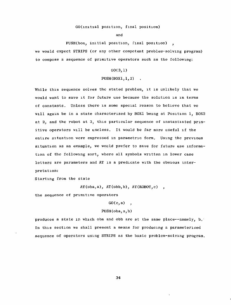
GO(initial position, final position)
and
PUSH(box, initial position, final position) ,
we would expect STRIPS (or any other competent problem-solving program)
to compose a sequence of primitive operators such as the following:
G0(3,1)
PUSH(30X1,1,2) .
While this sequence solves the stated problem, it is unlikely that we
would want to save it for future use because the solution is in terms
of constants. Unless there is some special reason to believe that we
will again be in a state characterized by BOX1 being at Position 1, BOX2
at 2, and the robot at 3, this particular sequence of instantiated prim-
itive operators will be useless. It would be far more useful if the
entire situation were expressed in parametric form. Using the previous
situation as an example, we would prefer to save for future use informa-
tion of the following sort, where all symbols written in lower case
letters are parameters and AT is a predicate with the obvious inter-
pretation:
Starting from the state
AT(oba, a), AT(obb,b), AT(ROBOT,c) ,
the sequence of primitive operators
GO(c,a) ,
PUSH(oba,a,b)
produces a state in which oba and obb are at the same place—namely, b.
In this section we shall present a means for producing a parameterized
sequence of operators using STRIPS as the basic problem-solving program.
34

b. Solving Parameterized Problems with STRIPS
There appear to be two distinct approaches to the problem
of producing a parameterized sequence of operators using the STRIPS
problem solver: We can use STRIPS to solve a specific problem and seek
ways to generalize the arguments of operators from constants to param-
eters, or we can generalize the problem statement so that it is in terms
of parameters only and seek ways to modify STRIPS so that it can solve
parameterized problems. Surprisingly, perhaps, the second of these two
approaches has proven to be the fruitful one. Following this approach,
the modification to STRIPS is as follows:
(1) Replace every constant in the description of
the initial state by a distinct parameter symbol.
(Multiple occurrences of the same constant lead
to differently named parameters.) For each
parameter symbol, create a "binding" that binds
it to the constant it replaces.
(2) Similarly, replace each constant in the goal
statement with a distinct parameter symbol.
Bind each parameter to the constant it replaces.
(3) When performing resolutions within QA3, parameters
obey the rules for parameter bindings as discussed
in Section II-A. However, no parameter is ever
actually replaced by its binding in a logical
expression. Instead, separate lists are used to
keep track of parameter bindings, and the logical
unification operation must be aware of this special
bookkeeping.
35

Upon completing the solution to a problem, STRIPS produces
a sequence of primitive operators whose arguments are parameters. If
all parameters bound to constants are in fact replaced by those constants,
we will have precisely the sequence of instantiated operators produced*
by the existing, unparameterized problem solver. Remarkably, the STRIPS
search for a solution to the parameterized problem is isomorphic to the
search for a solution to the unparameterized problem . Thus no more
effort is expended in producing the general solution than would be ex-
pended in producing the specific solution.
3. Construction of a Plan Description
Once STRIPS has solved a problem and generated a parameterized
plan, we can make it into a new complex operator to be added to the
existing repertoire of ILAs available to STRIPS as operators. To do
this, the complex operator must be characterized in the same fashion
as any other operator; we must construct a precondition wff, an add-
list, and a delete-list.
In order to extract the appropriate information from a plan
to make these constructions, we need the notion of a kernel state. A
kernel state is a collection of axioms constituting a subset of thet
axioms defining a given state. We intend to include in each kernel
*It is possible, even using the standard unparameterized STRIPS problem
solver, to produce as a final solution a sequence of operators that
are only partially instantiated.
Note that if we extract from a set s of axioms a subset k, then the
totality of worlds satisfying s is a subset of the totality of worlds
satisfying k. In other words, fewer axioms specify a more general
world.
36

state only those axioms relevant to fulfilling the goal. Figure 2 illus-
trates the situation we have in mind. STRIPS can produce both the se-
quence of (parameterized) operators OP ,...,OP and the sequence of1 n-1
(parameterized) states s ,...,s . The kernel states k ....,k are to
be computed. We first assume that the sequence of operator preconditions
have been labeled g ,...,g , and g is the final goal. The following
algorithm computes kernel states by beginning from the final state and
working backwards to the initial state.
OP.
OPn-1
TA-8973-1
FIGURE 2 SEQUENCE OF STATES ANDKERNEL STATES
37

Start:
Put in k exactly those axioms of s used in then n
proof of the overall goal g .n
Recursion:
Put an axiom in kernel k only if
(1) It is in s and used in the proof of thei
precondition of OP., or
(2) It is a member of k but is not on the add-i+l
list of OP .i
It is not difficult to prove that the following properties
are consequences of this algorithm definition:
(1) Each set k of kernel axioms is in fact a subseti
of the corresponding set s of state axioms.
(2) If a set of kernel axioms k is satisfied by a
configuration of the world, then application of
OP will produce a configuration of the world in
which kernel k is satisfied,i+l
In other words, if we are in a situation in which k is satisfied for
some i, then application of the remaining operators in the sequence
will result in a state in which the overall goal g is satisfied. Thus,
the sequence of kernel states k ,...,k defined by our algorithm serves
as a set of natural milestones for monitoring the execution of a sequence
of operators.
We may now complete the description of a complex operator
(from a plan generated by STRIPS), by using the following simple rules,
where s and s are respectively the initial and final parameterized1 n
states. (Note that the parameters in s and s are those resulting1 n
after making whatever substitutions were necessary in constructing the
plan.)
38

(1) The precondition wff is the conjunction of the
axioms in the initial kernel.
(2) The add-list consists of all axioms in s and
not in s .
(3) The delete-list consists of all axioms in s and*
not in s .n
By the definition of the kernels, if any set of kernel axioms is satis-
fied, then application of the remaining sequence of operators must lead
to a state in which the goal is satisfied; hence, Rule (1). Notice
that the add- and delete-lists are formed by set differences on the
initial and final states rather than set differences of kernels. This
is because these lists reflect all the (planned) effects of an operator
on the world, not just those effects that happen to be relevant to a
particular problem.
This rule is still somewhat tentative, but works well in "typical
situations.
39

IV VISION RESEARCH
A. Introduction
Three separate efforts are currently in progress in the area of
vision research. The first concerns the development of special-purpose
picture-processing routines needed for the intermediate-level actions.
The second conerns an exploration of the use of color and stereoscopic
information to obtain better-formed regions for general region analysis.
The third is an investigation of ways in which visual information ob-
tained during exploration can be used to build a world model; this work
is described in Appendix F.
These activities represent a dichotomy between short-range and
long-range plans for vision work. Our long-range plans continue to be
based on a region-oriented approach to general scene analysis. However,
we have encountered problems in getting the merging heuristics to func-
tion well in the corridor environment. In addition, the amount of com-
putation required for a general scene analysis is often excessive for
the limited amount of information required by the intermediate-level
actions. Thus, the special-purpose routines are being written to pro-
vide users of the robot with certain specific kinds of visual informa-
tion. Hopefully this information will be useful for more general scene
analysis programs as well, and thus the short-range effort will also
contribute to the long-range effort.
B. Vision Programs for Intermediate-Level Actions
The special-purpose vision programs basically perform only three
functions: orienting and locating the robot, detecting the presence
41

of objects, and locating objects. We shall consider each of these func-
tions in turn.
When the environment of the robot is represented accurately and
completely in the model, the chief role of vision is to provide feed-
back to update the robot's position and orientation. Angular orienta-
tion information is often needed in advance of a relatively long trip
down a corridor, where a small angular error might be significant. The
simplest way to obtain orientati-on feedback is to find the floor/wall
boundary in the picture, project it into the floor, and compare this
result with the known wall location in the model; any observed angular
discrepancy can be used to correct the stored value of the robot's
orientation.
For manuevers such as going through a doorway, both the robot's
position and orientation must be accurately known. This information
can be obtained from a picture of a known point and line on the floor.
Such distinguished points and lines are called landmarks, and include
doorways, concave corners, and convex corners. The basic program for
finding such landmarks has been described previously.6 The program has
undergone several refinements and improvements, and now works with the
model described in Section II-B of this report. Execution time is*
essentially the time required to pan, tilt, and turn on the camera.
Concurrently, the accuracy is limited by mechanical factors to between
5 and 10 percent in range and 5 degrees in angle. Increased accuracy,
if needed, can be obtained by improving the pan and tilt mechanism for
the camera.
*Since the camera, television control unit, and television transmitter
draw a large amount of power from the batteries, they are normally off.
Approximately ten seconds is required from the time these units are
turned on to the time that a picture can be taken.
42

Before the robot starts a straight-line journey, it may be desirable
to check that the path is indeed clear. A simple way to do this is to
find the image of the path in the picture and examine that trapezoidal-
shaped region for changes in brightness that might indicate the presence
of an obstructing object. This is a simple visual task, and a program
implementing it has been written. In its current form the program uses
the Roberts-cross operator to detect brightness changes. When we first
ran the program, we were surprised to discover that at steep camera
angles the texture in the tile floor can be detected and give rise to
false alarms. This is an instance of a major shortcoing of special-
purpose vision routines, namely, the failure of simple criteria to cope
with the variety of circumstances that can arise. This particular
problem can be solved by requiring a certain minimum run-length of
gradient. However, shadows and reflections can still cause false alarms,
and the only solution to some of these problems is to do more thorough
scene analysis.
If there is reason to believe that an object is in a given area,
but its location is not known exactly, vision can be used to locate the
object. We are currently working on an object location routine that
will
• Use the model to compute the image of the floor area
• Delete all but the floor area from the picture
• Use the region-merging routines to partition the floor area
into regions
• Inspect these regions to find the faces of the object
that touch the floor
• Calculate the coordinates that locate the object.
43

This is the most complicated of the special-purpose vision programs.
By making use of the model to exclude extraneous data and limiting
attention to finding merely the points where the object meets the floor,
we hope to obtain an efficient, reliable, and still useful special-
purpose vision routine.
C. Techniques for General Scene Analysis
For the past 18 months, we have based our work in general scene
analysis on the partitioning of the digitized picture into regions.7?8
If this partitioning is substantially correct, there are several ways
to identify the regions and complete the analysis of the scene.e>s>9
Unfortunately, it has not been possible to obtain reliable partitioning
in the corridor scenes. Regions that we wish to keep distinct—such as
two walls meeting at a corner—are frequently merged, and fragments of
meaningful regions that should be merged are too often kept distinct.
There are several ways in which this problem can be attacked. One
is to try to improve the quality of the input data. Another is to seek
improved merging heuristics. Another is to guide the merging by more
a priori knowledge, such as the fact that real region boundaries are
straight, and many edges are vertical. Another is to guide the merging
by feedback from recognition of parts of the scene. One can even con-
sider using the information in the model to compute an expected parti-
tioning, and turn to confirming, augmenting, and/or rejecting the hypoth-
esized partitioning.
Of these possibilities, we have concentrated on the first two.
One of the more promising ways of obtaining better input data is through
the use of color. When we explored color previously,10 we encountered
problems chiefly because of the low sensitivity of the vidicon sensor,
the low saturation of most of the colors encountered in the real world,
44

and the sensitivity of color measurements to such factors as the type
of ambient light, specular reflections, shadows, the dynamic range, and
nonlinearities in the camera tube.
To attack these problems and gain the advantages of color infor-
mation, the following program has been initiated and is now being car-
ried out:
(1) The vidicon has been replaced by a plumbicon, resulting
in an approximately ten-fold increase in sensitivity.
(2) A set of color filters has been selected and experimentally
checked. The filters match both the spectral transfer
characteristics of the plumbicon and the spectral charac-
teristics of the fluorescent lights used in the laboratory
and the corridors.
(3) An effort has been made to obtain adequate discrimination
with unsaturated colors covering a wide range of objects
in the laboratory. These colors range from pastels to
unsaturated but deep reds, greens, etc. It appears that,
with appropriate adjustment of the camera characteristics,
such discrimination will be adequate under most operating
conditions.
(4) A subsidiary investigation is planned to automatize the
iris control of the camera, such that the dynamic range
is automatically adjusted as a function of varying light
level of a scene. A fairly simple program will be written
to read one picture, analyze the distribution of light
levels, adjust the iris setting, and repeat the process
until a satisfactory distribution is obtained.
45

(5) The Fennema-Brice region analysis program has been
modified to accept color data. In addition, an alter-
native approach to region analysis tailored to the charac-
teristics of color data is being developed. Although
several test pictures have been taken and analyzed, this
work is still in a formative stage and requires further
investigation.
Another area that is being investigated is the use of stereoscopic
information to aid scene analysis. This study assumes that correspond-
ing vertex points in stereo pairs can be identified, and that the range
to these points can be computed. The basic question concerns the use
of this information in detecting and correcting errors in partitioning
the picture. One of the early observations was that this kind of in-
formation can detect errors and suggest corrections, but it can not
detect all errors or yield unique corrections. For example, if Figure
3(a) is an imperfect representation of part of a box, they by knowing
the range to the vertices of region A one will conclude that the region
is not planar. However, as the other constructions in Figure 3 illus-
trate, no unique correction of the errors is possible. Nevertheless,
if a list of possible corrections can be obtained, one can try to see
which one best explains the original picture data. (This is essentially
the line proposer and verifier technique suggested by Minsky and inves-
tigated by Griffith.11) Hopefully, the improvements provided by color
or stereo information will allow us to attack the more interesting,
higher-level problems in scene analysis.
46

(a) (b)
\ \
\ \\\
(c) (d)TA-8973-3
FIGURE 3 SOME POSSIBLE WAYS OF CORRECTING ANIMPERFECTLY PARTITIONED PICTURE
47

V HARDWARE AND SYSTEMS SOFTWARE
A. Introduction
The work of the systems group can be divided into three parts:
hardware modification and addition, monitor and diagnostic programs,
and user support programs. The first section deals with hardware, and
includes discussion of problems as well as current additions and future
modifications. The second section treats diagnostic programs and moni-
tor modifications. The third section discusses user programs and their
relation to existing hardware.
B. Hardware
The AI computer system is pictured in Figure 4. The dotted figures
and connections are future additions; the solid lines indicate existing
equipment. The left side shows the PDP-10 and its peripherals, the
right side the PDP-15 complex.
Changes in the past six months include:
• Moving two DECtape units from the PDP-15 to the PDP-10.
It is still possible to use these on the PDP-15 by switch
control.
• Modifying the TV interface from manual control to program
control.
• Modifying the robot.
The robot was adjusted to fix slippage in the wheels. A new gear
is on order to fix the pan motor. A new sensor was added, which enables
49

CO
CO
QCLU
OuQ.
Ooc
LUO
a
LU
O
LL
CO
LUcc
50

the robot to generate an interrupt (which is ovemdable) when it loses
contact with an object that it was pushing. Built into this sensor is
an interrupt capability which is triggered when the robot tries to push
against something that is too heavy for it (e.g., a wall).
During the past period it was determined that the DA25 interface
was unsatisfactory because the transfer rate was too slow. The maximum
rate that could be hoped for is one 18-bit word every 8 |j.s. In fact,
due to a design flaw, the best we have been able to obtain is a word
every 12 |is, and this is maximum rate. Average rate is closer to 16 |is.
Since we shall eventually require speeds approaching a word per
microsecond, we entered into negotiation with DEC. The resulting design
of the DA28 was a result of our joint efforts, and meets our needs. It
is to be delivered to SRI in August.
Another new development is the future receipt of the TENEX system.
This is a system designed and implemented by BBN to convert the PDP-10
into a paged machine. This will greatly increase throughput. The sys-
tem includes both hardware and software.
The hardware includes a paging box and certain modifications to the
PDP-10 CPU. These modifications are being made now.
Design specifications have been developed by us for an interface
between the IMP remote host and the PDP-15. This is to enable us to
enter the ARPA network. This design has been let out for competitive
bids and we are evaluating them prior to awarding a contract to build
it.
The final hardware modification is another future development.
This is our device multiplexer. It is possible, in the future, that
devices as yet unspecified will be added to the system. Rather than
designing an interface to the PDP-15 for each device, a universal
51
interface is being built to multiplex these future devices, one of which
is a Grafacon, which we would like to use in conjunction with our display.
C. Diagnostic and Monitor Programs
The Systems Group completed checkout of the diagnostic programs
for the drum and display during the past six months. The drum diagnostic
exercises all tracks of the drum (reading and writing), both fixed and
random patterns. It checks timing and parity. It also turns out to be
a good memory diagnostic, when used in conjunction with other programs.
The display diagnostic enables the standard Adage diagnostic pat-
tern to be displayed and refresh rate and interrupt levels to be checked.
The major monitor modification was a new swapper. This uses the
drum as a swapping device (rather than the disk packs). Preliminary
study seems to indicate an average enhancement of response time of from
150 to 200 percent. We plan to optimize the code in hopes of getting
another 50 percent increase in user response time. We have decided not
to implement any files on the drum, since the entire system will be
changed with the advent of TENEX.
Some modifications to the LOGIN and LOGOUT routines were implemented.
This gave a clearer picture of where most of the time was spent, and
which users were spending it.
The monitor was modified to handle the PDP-15 as a sharable device.
The PDP-15 peripherals (i.e., robot, display, A/D converter) are handled
as single-user subdevices. Also the monitor was modified to handle TV
input. When a picture is to be taken, the monitor ensures that no
accesses to the disk pack will take place. It then allocates core to
the user area and acknowledges that a picture may be acquired. The
picture is read in through the TV A/D converter via the DF10 channel.
52

It is then written on a unique disk file in that user's area. The TV
is then released by the monitor, and that core allocated for the pic-
ture acquisition is returned to the available area.
Currently, we are learning about TENEX and its monitor. The first
job we hope to do on that monitor is to change its file-handling I/O.
It currently treats all tertiary file space as one large disk. We want
to have removable, separate disk pack software, thereby giving each
subproject a disk pack for its own files and allocating one disk pack
for systems and backup availability. We are also starting to consider
rewrites for the various parts of the system which will change under
TENEX—specifically TV interface, DA25 interface, and drum utilization.
D. User Support Programs
The most important user support programs that were written were
the robot programs in the,PDP-10 and PDP-15. They are described in
Appendix G, "Robot Communications Between the PDP-15 and the PDP-10."
The PDP-15 programs have been written entirely by the Systems
Group. This was necessary because existing DEC software was written
for the customer who had a stand-alone PDP-15. Our monitor (if such
it may be called) is efficient and compact. It appears that our pres-
ent 12K will be sufficient core memory on the PDP-15 for the immediate
future, but it is easy to visualize that amount as being too small.
Currently we handle the PDP-10 interface, robot, display, and A/D con-
verter programs.
The PDP-10 interface program always assumes that the PDP-10 is the
master and the PDP-15 the servant. Therefore if any information has
to go from the PDP-15 to the PDP-10, it must be asked for by the PDP-10.
Similarlym if the PDP-15 is sending a message and the PDP-10 decides to
initiate a transfer the other way, it takes priority, its message is
sent, and the original message is retransmitted afterwards.
53

All assembling of programs for the PDP-15 is done by an SRI-written
PDP-15 assembler on the PDP-10 and then transferred to the PDP-15 via
the DA25. This is much faster and does not interfere with existing
PDP-15 routines while the assembly is running.
The Adage display has been programmed so that a user on the PDP-10
writing in MACRO or FORTRAN can use it. This is described in Appendix
H, "User Display Software Memo," Currently, a higher-order implementa-
tion for use by LISP programmers is being done.
Two other user routines currently being written are an A/t> converter
routine, and a magtape-to-DECtape program.
54

REFERENCES
1. B. Raphael, "Research and Applications — Artificial Intelligence,"
Final Report, Contract NAS12-2221, SRI Project 8259, StanfordResearch Institute, Menlo Park, California (November 1970) .
2. G. W. Ernst and A. Newell, GPS: A Case Study in Generality and
Problem Solving (Academic Press, New York, N.Y., 1969).
3. T. Garvey and R. Kling, "User's Guide to the QA3.5 Question-Answering System," Artificial Intelligence Group, Technical Note15, Stanford Research Institute, Menlo Park, California (October
1969).
4. B. Raphael, "The Frame Problem in Problem-Solving Systems,"
Artificial Intelligence Group, Technical Note 33, Stanford ResearchInstitute, Menlo Park, California (June 1970).
5. L. Travis, "Experiments with a Theorem-Utilizing Program," Proc.
AFIPS 1964 SJCC, Vol. 25, pp. 339-358 (Spartan Books, New York,N.Y., 1964).
"6. R. 0. Duda, "Some Current Techniques for Scene Analysis," SRIArtificial Intelligence Group, Technical Note 46, Stanford Research
Institute, Menlo Park, California (October 1970).
7. L. F. Chaitin, et al . , "Research and Applications — Artificial
Intelligence," Interim Scientific Report, Contract NAS12-2221,SRI Project 8259, Stanford Research Institute, Menlo Park, California
(April 1970).
8. C. R. Brice and C. L. Fennema, "Scene Analysis Using Regions,"Artificial Intelligence, Vol. 1, pp. 205-226 (1970).
9. A. Guzman, "Decomposition of a Visual Scene Into Three-Dimensional
Bodies," Proc. FJCC, pp. 291-304 (December 1968).
10. L. S. Coles, et al . , "Application of Intelligence Automata to
Reconnaissance," Final Report, Contract F30602-69-C-0056, SRIProject 7494, Stanford Research Institute, Menlo Park, California
(November 1969) .
55

11. A. K. Griffith, "Computer Recognition of Prismatic Solids," Ph.D.
Dissertation, Department of Mathematics, Massachusetts Institute
of Technology, Cambridge, Massachusetts (June 1970).
56

Appendix A
A HEURISTICALLY GUIDED EQUALITY RULEIN A RESOLUTION THEOREM PROVER
by
Claude R. Brice and Jan A. Derksen
57
Appendix A
A HEURISTICALLY GUIDED EQUALITY RULE
IN A RESOLUTION THEOREM PROVER
ABSTRACT
A new way of handling the equality relation within the framework
of a resolution theorem prover is described. The system uses a modi-
fication of Morns' E-resolution, a rule of inference to handle equality,
controlled by heuristic tree search techniques. The modification makes
possible an implementation to which new rules of inference may be added
easily.
I INTRODUCTION
The equality relation is widely used but difficult to axiomatize
efficiently. We describe a new way of handling this relation within
the framework of a resolution theorem prover. The system uses a modi-
fication of Morns' E-resolution, a rule of inference to handle equality,
controlled by heuristic tree search techniques. The modification makes
possible an implementation to which new rules of inference may be added
easily.
Each time the resolution theorem prover makes an attempt to resolve
two clauses, but cannot unify a pair of literals, the "equality tree"
generator is called. A tree of clauses is built by substituting equal
terms in one of the literals, until unification is possible. The growth
of the equality tree is controlled by bounds on the processing time, the
59

breadth and depth of the tree, and a reluctance" function. The reluc-
tance function associates a cost with each node of the tree and selects
nodes for expanding with minimal cost. The function is a linear combi-
nation of several "features." Some of the features are the probability
that the literals will unify, the length of the literals, the number of
constants the literals have in common, and the length of the clauses in
which the literals occur.
Section II gives information on terminology, theoretical background
and completeness results for E-resolution and variants. Section III
describes the heuristic machinery of the system. It includes also
descriptions of the "equality tree" and the search strategies used to
find a path from the root to the goal node of the tree. Four sample
proofs are given in Section IV.
II E-RESOLUTION
It is assumed that the reader is familiar with the standard nota-
tion and terminology used in lierature on resolution.1 Among other
methods for dealing with equality, paramodulation is relevant as E-
resolution can be shown to be definable in terms of paramodulation with
resolution.1 Therefore, let us recall briefly the definition of
paramodulation.
Paramodulation—This is a rule of inference that, given two clauses:
A
and
a = p v B (or 3 - a v B) ,
*References are listed at the end of this appendix.
60

having no variables in common and such that A contains a term 5, with §
and ot having a most-general unifier a, forms A' by replacing in A one
single occurrence of 6 by p and infers A' V B .
Example: given the following three clauses
c = d V Qc
f(c) ^ f(d)
X = X
letting A correspond with f(c) ^ f(d), B with Qc, a = P with c = d, and
6 with d in A', then one can deduce by paramodulation the clause
f(c) ± f(c) V Qc
and, by resolution, the clause Qc.
Thus, intuitively, paramodulation provides a way to make use of the
substitutivity property of equality. The reflexivity property does not,
in E-resolution, require special axioms, and if a and 6 have no most-
general unifier, the program tries to find one for (3 and 6 (with the
same definition for y, 6> and p as in the paramodulation definition).
Each clause may generate many distinct paramodulators. One can define,
following Ref. 1, the descendants of a clause C from a set S obtained by
paramodulating into the literal & of C, in the following manner:
P (S,C,£) = (C} ,
P (S,C,jfc) - the set of descendants obtained from C ,
61

and by induction:
P (S,C,,C) = the set of descendants obtained by paramodulating from
k—1the clauses of P (S,C,1) into the literal j,
A. E-Resolution Defined
Using the preliminary definition above, one can define E-
resolution as follows:
oo kLet P (S,C,4) be the union of the P (S,C,&) for the different
values of k. C is an E-resolvent of two clauses C and C iff there3 1 2
exist a descendant clause C' from P (S,C ,1 ) and a descendant clause
C' from P°°(S,C ,H ) such that C is a resolvent of G' and c' and the
literals resolved upon in C7 and C7 are those descended from & and H ,1 £i \. £
respectively.
The intuitive idea behind these concepts is to be able to deal
with the transitive property of equality. The two clauses C and Ci. £
generate two trees of descendant clauses, and a path in one of these
trees can be built by a chain of equalities and substitutions. This
definition is of little help for programming purposes because of the
necessity of developing two trees of paramodulants. It can be shown
that a similar definition, but using only one tree, is equivalent. This
definition is given below:
C is an E-resolvent of two clauses C and C iff there3 1 2
exists G' from P (S,C ,j£ ) such that C is a resolventJL _L _L «j
of C and C and the literal resolved upon in C; is HJ - £ 1 1
or the descendant of H .
62

This way of implementing E-resolution differs from the one used in Ref.
3, but is closer to the formal definition of E-resolution given by
Anderson.1
B. Completeness for Ground E-Resolution
To show that this modified definition of E-resolution is com-
plete, we will show that it is complete for ground E-resolution and
following Ref. 1, lift this result to the general level. Using the
terminology of the first definition of E-resolution, let C be a resol-tJ
vent of the two clauses c' and c'. Let us denote G' by {&'} U L' and\. £1 J. 1_ _L
c/ by {&'} U L', where L' and L are the sets of literals from c' and£t £ &t \- £t J.
G' not deleted by the resolution. C is therefore expressed by I/ U L'£ o J. ^2and, since we have performed ground resolution, H, and & are comple-
1 £t
ments. By applying in reverse order to the literal H,' of the clause c',
the chain of equality replacements that took place to generate &', we
can generate the clause c" = {&"} U L" where Q," = ~Z . G" can then
resolve against C and as we apply the same chain of paramodulations,
the resolvent is C . It is shown in Ref. 1 that E-resolution, expressedO
here in terms of resolution and paramodulation, is complete with or
without set of support, under the same condition as paramodulation: If
the reflexivity axiom (FA(x) x = x) (in which FA(x) stands for (Vx)) is
present and all reflectivity functional axioms
(FA(x,y)(x = y ID f(x) = f(y))) are also present.
C. Comments on E-Resolution
If E-resolution can be expressed in terms of paramodulation
and resolution, one might wonder to what extent it is a useful technique.
In contrast with paramodulation, E-resolution limits the number of
clauses on which a theorem prover works. This is an important advantage
63

because the strategies used to select clauses that are resolved upon are
not very successful when the number of clauses increases. The reason
is that in E-resolution a clause is added to the set of clauses of the
system only if a resolvent is found, while in paramodulation the clauses
that would be on the intermediate nodes of the E-resolution tree would
be added. However, two clauses may yield more than one resolvent, and
E-resolution is complete only if from two clauses one can generate all
the possible distinct E-resolvents. To generate all the E-resolvents
from two clauses C and C , one would have to grow from C or C a tree1 £i \- £t
P (S,C ,H ) or P (S,C ,!i ) until all the possible distinct paramodulants.L J- £ £
of C or C into fa or i have been found. In practice, these trees are\- £t \. £t
almost never generated entirely. They could sometimes be infinite trees
and, at any rate, the expansion of these trees is time consuming. Fur-
thermore, in most cases not all the E-resolvents of two clauses are
needed to obtain a proof. Instead, as in Ref. 3, one might use a tree-
level bound on the depth of the E-resolution tree. This bound limits
the number of nodes to be generated, and it is increased progressively
until a proof is found. Of course, then some procedure to save the
partially expanded trees of paramodulated clauses should be implemented.
If a proof is not found, the tree-level bound is incremented and the
search can continue using the saved trees. This tree-level bound serves
also the purpose of limiting the search when it happens that two clauses
have no E-resolvents. To further limit the search, Morris's E-resolution
program3 was activated only if the two literals H and H of two clauses
C and C did not unify. Although this limitation seems fairly natural,1 £
it made the system incomplete, as was shown by Anderson1 using the fol-
lowing set of clauses:
(1) Pf(x)g(y) V Ph(x)i(y)
~Pf(a)g(b)
64

~ph(b)l(b)(4) f(a) = f(c)
(5) h(c) = h(b)
The only possible resolvents obtained, if E-resolution is called only
iff two literals do not unify, are:
Ph(a)i(b)
and
Pf(b)g(b)
However, by using the general E-resolution, one can generate the nil
clause:
(6) Ph(c)i(b) E-resolvent from (1) and (2) obtained by
paramodulation of (1) using (4)
(7) nil E-resolvent from (6) and (3) obtained by
paramodulation into (6) using (5).
D. The EQA3 E-Resolution System
The E-resolution program EQA3 was designed to be a package
that could be added to QA3.S QA3 is a question-answering system based
on the resolution principle, and it uses the set-of-support and unit-
preference strategy. EQA3 does not differ in principle from the system
described in Ref. 4 but actually suffers from its implementation in a
theorem-proving system whose conception and structure do not lend them-
selves to improvement and refinement. However, QA3 will probably be
rewritten or replaced by a more flexible theorem prover. With this
purpose in mind, we have tried to keep EQA3 as general as possible.
The descendant tree generator, which is the core of the system, could
65

eventually be used to generate any type of clause that could be inferred
using a rule other than paramodulation. For example, to express that
the predicate P(x,y,z) is such that the order in which its arguments
appear is irrelevant, one can use the tree generator with a rule of in-
ference consisting of a permutation of the arguments. Special permuta-
tions such as cyclic permutation can be used. For example, when the
orientation of a line is irrelevant, one wants to express that the two
predicates LINE(A,B) and LINE(B,A) have the same truth value. A predi-
cate may have only a few ground instances. A model for this predicate
could then be the list of the ground instances for which the predicate
is true. Each clause containing a model evaluable predicate can be re-
solved against or subsumed by a model unit clause.
One can imagine that the tree generator could select, de-
pending on the problem, different rules of inference to produce descen-
dant clauses. The selection can be simply as in E-resolution, e.g.,
the failure of rule 1 (resolution) implies the use of rule 2 (E-
resolution). Another possibility is that each predicate has a property
list that tells what rule of inference has to be used.
In its actual implementation, EQA3 makes use of an evaluation
function or reluctance function to select the next node to be expanded.
The system actually uses only paramodulation to infer new nodes in the
tree. Not all the descendants of clauses obtained by paramodulation
into a literal are generated. Some of them would be of no use in trying
to get an E-resolvent. The substitution takes place only in the terms
of the literal or descendant of the literal when the unification algorithm
fails. Thus, this implementation suffers from the same incompleteness as
Morris's system (see Section II-C), but this limitation has no practical
consequences. The reflexivity axiom X = X does not have to be added as
66

an axiom to the set of clauses. It is "built into the system and used
to resolve against inequality literals.
Each clause containing an equality literal is collected on a
list of equalities (EQLIST). This list is ordered by length of clause.
Thus equalities belonging to shortest clauses will be tried first for
possible application of the E-resolution rule. This was done in an
effort to keep the length of the eventual E-resolvent to a minimum (cf.
unit preference strategy).
The next section describes the structure of the tree generator
and the reluctance function in more detail.
Ill THE EQUALITY TREE
The essence of E-resolution is that each time two literals with the
same predicate but opposite sign do not unify, a special procedure is
invoked to show these two terms to be equal using unknown equalities.
The special procedure generates a tree of modified clauses obtained by
substituting terms in the literal of the clauses until they unify, using
a list of positive equalities. This tree is called the "equality tree."
The procedure is a rather general one given:
(1) A start node, a string of symbols, e.g., p(a).
(2) A goal node, also a string of symbols, e.g., p(b).
(3) A list of equalities, e.g., (a = c, c = b). We can
replace part of a string by another string known to be
its equal by a most-general common instance, and form
in this way other nodes (grow a tree), e.g., we can
form the nodes p(c) and p(b); the last node is equal
to the goal node.
67

The procedure tries to find a path between the start and goal nodes.
In our example the path found is p(a), p(c), p(b). In our description
we showed only nodes consisting of single literals. In general, nodes
have more complex values (clauses), although the search is done for
specific literals in the start and goal clauses.
A. Search Procedures
Several difficulties arise if we want to implement such a
procedure:
(1) A path between two nodes does not have to exist; •
in this case we should be able to end the search.
(2) Some branches of the tree must be recognized as
unsuccessful, and the search stopped in favor of
other branches.
Because of such problems, we cannot use a "depth-first" search technique
as we are unable to recover from a single wrong decision in an infinite
tree, e.g., we grow a branch from the node f(x) = e * x and repeatedly
apply the equality x = e * x. Then we get the branch
f(x) = e * x
f (x) = e- * e * x
f(x) = e * e * e * x
68

An alternative, is a breadth-first search; we avoid the difficulty
associated with infinite branches, but now we cannot use heuristic in-
formation in deciding which branch to develop first.
The method used in this system is search controlled by a re-
luctance function. In this method we may think of a "frontier" of those
nodes whose successors have not been examined. This frontier is extended
by choosing any node in it and examining the node's successors. The
node chosen will be that which has the minimum value of some function
called a "reluctance function." It is easy to see that breadth-first
and depth-first search are special cases of this last search method.
B. How to Grow a Tree
Several factors have to be considered when growing a tree.
(1) Control of the size of the tree; there are bounds
on:
• Breadth
• Depth
• Processing time spent working on this
specific problem.
(2) Successors or sons of the node. Not all of the
sons of a node are developed at once because
the number of sons may be unreasonably large,
for instance, when a long list of equalities
has to be used. Also, we may reach a goal node
without having to find all the successors.
(3) Some nodes are thrown away if associated cost
values are above a "cutoff" criterion. In
69

our system this is a limiting of the length of
the literal relative to the length of the goal
literal used. If the global variable LIMIT
LENGTH is set to four, then any node with
literals whose number of symbols (length) is
four times the length of the goal literal will
be thrown away.
(4) Order of the evaluation of the nodes, the re-
luctance function: the essential function is
EVALCOST.
The tree-growing program is written in an elegant recursive
form as suggested by Burstall.5 The controlled search therefore could
be programmed in a manner very similar to depth-first search.
C. The Reluctance Function
Each time a node is to be selected for expanding, the candi-
dates are "open" nodes--nodes that do not have their maximum number of
sons (limited by the breadth bound). The node selected is the one with
minimal associated cost. The reluctance function should have a minimal
value for the chosen node. The cost given by the reluctance function
"EVALCOST" is a combination of several "features." A feature f is a
function that measures some properties of a node. EVALCOST makes use
of the linear combination
C = C f + C f ... + C f11 22 n n
Of course, nonlinear combinations are possible, but for our system the
linear reluctance function is adequate.
70

D. Features Used in the Reluctance Function
The features are all functions of the string (literal) asso-
ciated with the node under investigation. The goal literal is the
string that is the ultimate goal of the tree search. The features are:
(1) Length relative to the length of the goal literal
(2) Number of constants in common with the goal
literal
(3) Number of function symbols in common with the goal
literal
(4) Degree of nesting relative to degree of nesting
of the goal literal
(5) Length of the clause of which the literal is an
element
(6) Probability that the literal and the goal literal
will unify.
E. Detailed Description of the Features
(1) Length: number of symbols in the string (literal)
including parentheses, e.g., (f(e)3) -• 7.
(2) Number of constants: A list of constants occurring
in the literal is made and compared with the list
of constants occurring in the goal literal. An
integer expressing the number of shared constants
is computed. The algorithm gives, in this way,
a maximal value for literals with an equal number
of the same constants, while lower values are
71

obtained for a smaller or larger shared number of
constants.
(3) Number of function symbols: each substring of
the form '((atom) (atom or list)1 contains the
occurrence of a function symbol, here, '(atom)'.
The procedure for the number of constants is re-
applied, this time with the two lists of function
symbols.
(4) Degree of nesting: this feature is defined as
£ K , where x is an element of the string under
consideration; x is not '('or')'; K is the numberx
of bracket pairs enclosing x—e.g., '(g(f a)(e))' -* 7.
(5) Length of clause: the literal associated with
the node is an element of a clause. The resolu-
tion system has a built-in strategy with a
preference for short clauses. In the E-resolution
part, too, nodes with long clauses are penalized.
(6) Probability that the literal and the goal literal
will unify: normally if two literals do not
unify, the unification algorithm fails and leaves
us without information on how "well" the unifica-
tion was doing. If the algorithm in this system
fails, it reports the degree to which the laterals
did match. The algorithm adds
• For each term that matches [I/number of
terms], the weight of the term, to a
running count
72

• Inside a term, for each subterm, [weight
of the term/number of subterms] to the
running count.
The algorithm tries to unify the two literals and
adds each time that the unification succeeds on a
subterm the weight of the term or subterm of a
term to the running count, e.g.,
(P(f x)(a)), (P(g x)(a)) - 0.5
(P(f x)(a)), (P(f y) z) - 1
(P(f(a))x), (P(f(b))(a)) - 0.25
F. Performance of EVALCOST
Not much is known about the influence of the different features.
The sample runs are made with a setting in which the length of the
literal, and to a lesser degree the length of the clause of a node, de-
termine the expansion of the tree. The user will have to experiment
which setting to use for each problem. A semi- interactive use with
tracing, printing, and checking of the growth of the tree seems the best
approach.
G. Structure of the Tree
1. Structure of the Tree
The tree is built with atoms generated by GENSYM. Each
node has a property list with the following flags and information:
VALUE, the literal associated with the node
FATHER, a backpointer to the father node
73

SONS, a list of pointers to son nodes
EXPBY, a pair of pointers to the terms of the
literal and the equality, used in the substitution
TERMINAL, T if node is terminal, otherwise NIL
BOUND, dotted pair of current depth and breadth
(number of sons) (in this order)
COST, cost as computed by EVALCOST.
2. An Example of a Small Tree'
START
G0001
((FATHER START)
(SONS NIL)(TERMINAL NIL)
(BOUND.(1.2))(COST 15))
((FATHER NIL)(SONS.(G0001 G0002))
(TERMINAL NIL)(BOUND.(0.0))(COST 10))
G0002 ((FATHER START)(SONS.(G0003))
(TERMINAL NIL)(BOUND.(1. 2))
(COST 9))
G0003 ((FATHER G002)(SONS NIL)
(TERMINAL NIL)(BOUND.(2.1))
(COST 0))
IV EXAMPLES OF RUNS
Three of the following examples come from elementary group theory.
'*' denotes the binary group operator. E denotes the identity of the
group and INV denotes the inverse operator. One example is about the
induction proof for the synthesis of the reverse function. REV denotes
the reverse function, and AP, LIST, and CDR denote the LISP functions
APPEND, LIST, and CDR. For each proof that implied only one E-resolution,
the penetrance—the number of nodes developed on the path divided by the
74

total number of nodes developed in the tree—is given. In the sample
runs the theorems to be proven are preceded by TQ and the axioms by AX.
Literals derived by E-resolution from a part of the negation of the
theorem are preceded by NEG-THM.
Example 1. (See sample printout on page 72). The theorem
proven is: the identity element of a commutative group is
unique. The negation of the theorem is (el * x = x) &
el ^ e, or in prefix notation as used in the printouts:
= (*(E1,X)X) & (E1,E). EQA3 generates a contradiction
by paramodulating into ^ (E1,E) and resolving against the
reflexivity axiom = (X,X). A measure of goal directedness
of the proof is the ratio of the length of the path and
the total number of nodes generated during the proof.
This measure is called penetrance. The penetrance in
example 1 was 3/8.
Example 2. In the proof shown on page 73 the group is re-
stricted such that for all elements X, (X(* X X)E). The
theorem proven is (Vx) x-x = e. Penetrance 8/22.
Example 3. Page 74 gives a sample printout for the proof
of the theorem (Vx)(Vy)(Vz)x-(y-(x -y )) = e. The
penetrance was extremely low, 7/104. It seems that the
main reason for such a bad performance was the great
number of unproductive paramodulants that were generated
by using the commutativity axiom (FA(X,Y)(=(* X Y)(* Y X))).
Example 4. In the sample printout on page 75, SK45, SK46,
and SK47 denote the constants that replace the universally
quantified variables Yl, Y2, and X. As the system starts
from the negation of the theorem to find a contradiction,
75

the universal quantifiers of the theorem become existential
quantifiers and the variables are replaced by Skolem con-
stants. The instantiation of Y2*, not given by the system,
is Y2* = AP(LIST(CAR(SK45)),SK46)) or for all Yl, Y2, and
X the theorem is true with Y2* = AP(LIST(CAR(Y1),Y2)).
Penetrance 3/5.
V CONCLUSION
After some experimentation with our implementation of the equality
rule several things became clear to us:
(1) An equality rule without any guidance is doomed to
fail on any nontrivial problem.
(2) A heuristically guided search gives good results
for a limited class of problems for which the reluc-
tance function features are properly "tuned."
(3) For a wider range of problems, watching the theorem
prover in the process of proving an equality and
introducing simple special rules of inference in
case of failure or bad performance turns out to be
the best solution.
76

(PAS)EXECUTIVE M0DF
-RESET
- A X C A X 1 AX2)AX1 CFA (X Y) (= (* X Y) C* Y X»)AXI0M
AX? CFA CX) ( = (* F X) X))AXIOM
- T Q ( I F C F A C X > < = ( * El X) X»<= Fl F»
1. NEG-THM 0. = <*<£ ! ,X> ,X>
2. NFG-THM 0. -=CF1,E)
3. NFG-THM 0. -= (*( E, El >, E)
CLAUSE 3. EQUAL.
4. NEG-THM 0. -= <*< El, E), E)
CLAUSE 4. EPUAL.
5. NFtt-THM 0. -=<E, F)
CLAUSE 5. EQUAL.
6. AXI0M 0. = ( X * X )
7. PFSC5. 6.) 1. CONTRADICTION
YFS
Example 1
77

( O A S >EXECUTIVE M0DE
-PESET
«-AX(AX2 AX3 AX4 AX5)AX2 (FA CX) ( = C* E X) X))AXI0M
AX3 (Fft (X) (= <* X X) E))AXI0M
AX4 (FA (X) (= (* X ( I N V X>> E))AXI0M
AX5 (FA (X Y 7.) ( = (* X (* Y Z>> (* (* X Y) Z > > >AXI0M
- T f > ( F A ( X ) ( = X ( I N V X ) ) )
1. NEG-THM 0. -=(SK45, INV(SK45»
?. NEG-THM 0. -=(SK45,*(E,INV(SK45»>
CLAUSE ?. EOUAL.
3. NEG-THM 0. -= ( SK45, *(*(X, X), I N V ( SK 45) ) )
CLAUSE 3. EOUAL.
4. NFG-THM 0. - = ( SK45,*(Y* *(Y» I NV( SK45) ) »
CLAUSE 4. EQUAL.
5. NEG-THM 0. -= (SK45»*( SK45, E))
Q.AUSE 5. EQUAL.
6. NFG-THM 0. - = ( SK45, * ( SK45* *(X» X) ) )
CLAUSE 6. EPUAL.
7. NEG-THM 0. -= ( SK45, *(*( SK45* Z), 7.) )
CLAUSF 7. EOUAL.
R. NEG-THM 0. -= (SK45* *( E, SK^5) )
CLAUSF R. EOUAL.r
9. NEG-THM 0. -= (SK45, SK45)
CLAUSF 9. EOUAL.
1 0 . A X I O M 0 . = ( X , X >
11.RFS(9. 10.) 1. C0NTPADICTI0N
YFS 78
Example 2

EXECUTIVE M0DE
-PFSET
-AX(AX1 AXP AX4 AX5)AX1 (FA CX Y) ( = (* X Y) (* Y X>»
AX? (FA (X) (= (* E X) X))AX T 0M
AX4 (FA (X) (= (* X (INV X)) E»AXIOM
AX5 (FA (X Y Z> (= (* X (* Y Z>> (* (* X Y) Z»>AXI0M
-T"(FA(X Y ) ( = E (* X(* Y(* (INV XXINV Y))»»
1. NEG-THM 0. -=(E.»*(SK45**(SK46** . ( INV(SK45)* INV(SK46) )) »
?. NFG-THM 0. -=(E**(*(SK46,*( INV(SK45), INV(SK46)»* SK^5))
CLAUSE 2. EOUAL.
3. NFG-THM 0. -= ( E, *(*( SK46, *( I NV( SK 46) * I NV( SK/t5» ) , SK45) )
d.AUSF 3. FOUAL.
A. NEG-THM 0. -=(F,* f*(*(SK46* INV(SK46))» INV(SK45)>* SK45))
CLAUSE A. FOUAL.
5. NEG-THM 0. -=( E, *(*(£, I NV( SK45) )* SK45) )
CLAUSE 5. FOUAL.
6. NEG-THM 0. -= ( E* *( INV( SK 45) , SK45) )
CLAUSE 6. EOUAL.
7. NFG-THM 0. -= ( E, *( SK45* INV( SK45) ) )
CLAUSE 7. EOUAL.
8. NEG-THM 0. - = (F, E)
CLAUSF R. EOUAL.
9. AXI0M 0. =(X,X)
10.RFS(R. 9.) 1. C0NTRADICTI0N
Example 3
79

E X E C U T I V E M0DF
-AX(AX? AX3)AX2 (FA (U V W) (= (AP U (AP V W) ) (AP (AP II V) W) ) )A X I O M
AX3 (FA (U) (IF (N0T (NULL U)) (= (PF.V U) (AP ( R E V (CDR U» ( L I S T (CAP U ) ) ) ) ) )AXI0M
-TPR0VF 01(FA (Yl Y2 X) ( IF ( A N D (N0T (NULL Y l ) ) (= (AP ( R E V Yl ) Y? ) ( R E V X»)(FX (YP*> (= (AP ( R E V (CDR Y l ) ) Y2*) (RFV X ) ) ) ) )1. NEG-THM 0. -NULL(SK45)
£• NEG-THM 0. = ( A P ( R E V ( SK 45) * SK^6) , RFV( SK
3. NFG-THM 0. - = ( A P ( R E V ( CDP( SK ^55) )* Y2*) * R F V ( SK 47) )
4. NFG-THM 0. - = ( A P ( R E V ( C D R ( S K 45) )* Y2*) * A P ( R F V ( SK45) , SK 46) )
CLAUSF 4. EQUAL.
5. NEG-THM 0. - = C A P ( R E V ( C D R ( S K 4 5 ) ) , Y 2 * ) , A P ( A P ( R E V ( C D R ( S K 4 5 ) ) , LI S T ( C A R ( S K 4 5 ) ) ) , S K 4 6 ) ) NULL (SK 45)
CLAUSE 5. EQUAL.
6. NEG-THM 0. - = ( A P ( R E V ( C D R ( SK45) ) , Y2*), AP( REV( CDR( SK 45) ) , A P ( LI S T ( C A R ( S K 4 5 ) ) , S K 4 6 ) ) ) NULL (SK 4 5)
CLAUSE 6. EQUAL.
7. A X I 0 M 0. = ( X * X )
R. RES(6 . 7.) 1. N U L L ( S K 4 5 )
9. PFSd. 80 2. C O N T R A D I C T I O N
YES
Example 4
80

REFERENCES
1. R. Anderson, "Completeness Results for E-Resolution," Proc. Spring
Joint Computer Conference, pp. 653-656 (1970).
2. T. D. Garvey and R. E. Kling, "User's Guide to QA3.5 Question-
Answering System/' Artificial Intelligence Group, Technical Note
15, Stanford Research Institute, Menlo Park, California (December
1969).
3. J. B. Morris, "E-Resolution: Extension of Resolution to Include
the Equality Relation," Proc. International Joint Conference on
Artificial Intelligence (Association for Computing Machinery,
New York, New York, 1969).
4. C. C. Green, "The Application of Theorem Proving to Question-
Answering Systems" (thesis) Artificial Intelligence Project Memo
AI-96, Stanford University, Stanford, California, pp. 123-130
(June 1969).
5. R. M. Burstall, "Writing Search Algorithm in Functional Form,"
Machine Intelligence 3, D. Michie (ed.) (Edinburgh University
Press, Edinburgh, Scotland, 1968).
6. R. J. Popplestone, "Beth-Tree Methods in Automatic Theorem Proving,'
Machine Intelligence 1, N. Collins and D. Michie (eds.) (American
Elsevier Publishing Co., New York, New York, 1967).
7. G. A. Robinson and L. Wos, "Paramodulation and Theorem Proving in
First Order Theories with Equality," Machine Intelligence 4,
B. Meltzer and D. Michie (eds.) (American Elsevier Publishing Co.,
New York, New York, 1969).
81

Appendix B
REASONING BY ANALOGY AS AN AID TO HEURISTICTHEOREM PROVING
by
Robert E. Kling
83
Appendix B
REASONING BY ANALOGY AS AN AID TO HEURISTIC
THEOREM PROVING
ABSTRACT
When heuristic problem-solving programs are faced with large data
bases that contain numbers of facts far in excess of those needed to
solve any particular problem, their performance rapidly deteriorates.
In this paper, the correspondence between a new unresolved problem and
a previously solved analogous problem is computed and invoked to tailor
large data bases to manageable sizes. This appendix describes a particu-
lar set of algorithms for generating and exploiting analogies between
theorems posed to a resolution-logic system. These algorithms are be-
lieved to be the first computationally feasible development of reasoning
by analogy to be applied to heuristic theorem proving.
85

Any contemporary heuristic deductive theorem-proving system that
proves theorems by applying some rules of inference to an explicit set
of axioms must use a carefully tailored data base. Most search pro-
cedures will generate many irrelevant inferences when seeking the proof
of some nontrivial theorem even when they are given a minimal set of
axioms. Generally, the effective power of a search procedure is limited
by the memory capacity of a particular system: most theorem provers run
out of space (absorbed by irrelevant inferences) before they run out of*
time when they fail to prove a hard theorem.
Consider a particular theorem P that can be solved with a set of
axioms D. Suppose that a theorem-prover S can prove P within its memory
limitations. Suppose D is expanded to D; by adding axioms that include
many of the same relations that appear in D. If S attempts P again, it
will generate many new irrelevant inferences that are derived from the
axioms in D' - D. In fact, the size of D need not be too much larger
than that of D to render P unprovable by S. Typical theorem provers
work with a D composed of less than 20 axioms. If P is hard for S, then
just a few additional axioms may add a sufficient number of inferences
to the search space to exhaust the memory before a solution is found.
In the '60's, most research focused on the organization of S and the
development of a variety of ever-more-efficient search procedures. Con-
sequently, researchers could choose an optimal D for each particular
theorem without sacrificing their research goals. In contrast, as
heuristic deductive systems are being proposed to solve real-world
problems, such as robot manipulation,3 larger nonoptimal data bases are
necessary.
*This observation is based upon my own experience with resolution systems
and is corroborated by other researchers using different paradigms.1 >3*
tReferences are listed at the end of this appendix.
86

Suppose we have a theorem P, and a large data base D . In general,
there is no way to choose a small subset D of D' such that D =*»P. Sup-
pose we had previously solved some theorem P that is analogous to P in
so far as analogs of the axioms used in the proof of P will be required
in the proof of P. If we could generate the analogy between P and P to
find the set of axioms and use them as D , then we could let S attempt
P with greater hope of success. This appendix describes a set of al-
gorithms for generating an analogy between some given pair of P and P
and for exploiting this relationship to estimate D'.
The preceding discussion has been rather general and applies to any
heuristic theorem prover such as LT2 and resolution.4 However, each
paradigm will require slightly variant representations and methods for
generating and using analogical information. Effective research demands
working with a specific theorem prover; for reasons of convenience, I
have chosen QA3,5 a resolution-based theorem prover. QA3 and the al-
gorithm ZORBA-I, described below, are implemented in LISP on a PDP-10
at Stanford Research Institute.
Before describing ZORBA-I abstractly, I want to exemplify the kinds
of theorems that it tackles. Briefly, they are theorem-pairs in domains
without constants (e.g., mathematics) that have close to one-to-one
analogies. The theorems include those that are fairly hard for QA3 to
solve even with an optimal memory. For example, ZORBA-I will be given
the proof of the theorem
T . The intersection of two abelian groups is an abelian group,
and is asked to generate an analogy with
T . The intersection of two commutative rings is a commutative£t
ring;
87

or, given
T . A factor group G/H is simple iff H is a maximal normal sub-3
group of G,
and its proof, ZORBA-I is asked to generate an adequate analogy with
T . A quotient ring A/C is simple iff C is a maximal ideal in A.4
None of these theorems is trivial for contemporary theorem provers. T
has a 35-step proof and T has a 50-step proof in a good axiomatiza-O
tion. A good theorem prover (QA3) generates about 200 inferences in
searching for either proof when its data base is minimized to the 10 to
15 axioms required for each proof. If the data base is increased to 20
to 30 reasonable axioms, the theorem prover may generate 500 to 600
clauses and run out of space before a proof is found. Note also that
the predicates in the problem statement of these theorems contain only
a few of the predicates used in the proof. Thus, T can be stated
using only the predicates {INTERSECTION; ABELIAN], but a proof, in
addition (GROUP; IN; TIMES; SUBSET; SUBGROUP; COMMUTATIVE}. Thus, while
the first set must map into [INTERSECTION, COMMUTATIVERING], the second
set can map into anything.
Figure B-l shows a relational space R covering all the relations
in the data base. Let R' and R' be the set of relations in the state--L £
ments of the new and old theorems (T and T , for example). In addi-
tion, we know the relations R in some proof of T (since we have a
proof at hand). We need to find the set R that contains the relations£t
we expect in some proof of T , and we want a map Q: G(R ) = R .^ 1 2i
Clearly, a wise method would be to find some Q', a restriction of
G to R' such that G'(R ) = R', and then incrementally extend G' to G',J- J. £ 1
G', ... each on larger domains until some G'(R ) = R . ZORBA-I performs^ 1 2
in such a way that each incremental extension picks up new clauses that
88

TA-8973-4
FIGURE B-1 VENN DIAGRAM OF RELATIONS IN STATEMENTS T, TA, AND D
could be used in a proof of T . In fact, if we get no new clauses from
an extended Q', that may be reason to believe that G' is faulty. I nowJ J
will describe the generation algorithm in more detail.
The user presents ZORBA-I with the following information:
(1) A new theorem, T , to prove.
(2) An analogous theorem, T (chosen by the user), that has
already been proved.
(3) Proof [T]} which is an ordered set of clauses C suchK
that Vk, C is eitherk
(a) A clause in —i T
(b) An axiom
(c) Derived by resolution from two clauses
c and c j < k and i < k.J
89

These three items of information are problem-dependent. It accesses
a large data base which includes more axioms than it needs for T or TA
and is, in this sense, problem independent. In addition, the user
specifies a "semantic template" for each predicate in his language.
This template associates a (semantic) type with each predicate and
predicate-place and is used to help constrain the predicate mappings to
be meaningful. For example, (STRUCTURE SET OPERATOR) is associated with
the predicate "group." Thus, ZORBA-I knows that "group" is a structure,
"A" is a set, and "*" is an operator when it sees group [A;*]. Currently,
the predicate types (for algebra) are STRUCTURE, RELATION, MAP, and
RELSTRUCTURE; the variable types are SET, OPERATOR, FUNCTION, and OBJECT.
ZORBA-I can make up a description descr[c] of any clause c according
to the following rules:
(1) V If P and -i p appear in c, then impcond[p] e descr[c].P
(2) V If p appears in c, then pos[p] e descr[c].P
(3) V If —i p appears in c, then neg[p] e descr[c].P
Thus, the axiom, "every abelian group is a group," e.g.,
V(x *) abelian [x;*] =s»group [x;*] ,
is expressed by the clause
—i abelian [x;*] V group [x;*] ,
which is described by
neg [abelian]; pos [group]
90

The theorem, "the homomorphic image of a group is a group/' e.g.,
V (X Y *i *2 cp)
horn [cp;X;Y] A group [X;*
=>group [Y;*2] ,
is expressed by the clause
-i horn [cp;X;Y] V -, group [X;* ] V group [Y;* ]_L £
and is described by
neg [horn], impend [group]
The semantic templates are used during both the INITIAL-MAP (when
the predicates and variables in the theorem statements are mapped) as
well as in EXTENDER, which adds additional predicates needed for the
proof of T and a candidate set of axioms for the data base. The clauseA
descriptions are used only by EXTENDER.
The INITIAL-MAP uses a rule of inference called
ATOMMATCH[atom 1; atom 2; ANA], which extends analogy by adding the
predicates and mapped variables of atom and atom to analogy ANA.*
ATOMMATCH now limits ZORBA-I to analogies where atoms map one-to-one.
But a slight generalization of ATOMMATCH can be made so that ATOMMATCH
can accept many-many maps of atoms. INITIAL-MAP is a sophisticated
search program that sweeps ATOMMATCH over likely pairs of atoms, one
Atoms, not predicates.
91

from the statement of T, the other from the statement of T . Alterna-A
tive analogies are kept in parallel (no backup), and INITIAL-MAP termi-
nates when it has found some analogy that includes all the predicates*
in theorem statements. Usually, this is the only analogy generated.
EXTENDER accepts a partial analogy G generated by INITIAL-MAP and
the (unordered) axioms used in the proof P. In addition, EXTENDER has
access to the data base D used by the theorem prover. It partitions
this axiom-list, called AXLIST, into three distinct subsets, ALL, SOME,
and NONE (AXLIST = ALL U SOME U NONE).
If all the predicates on an axiom Ax are in G , ax e SOME; and ifK J. K
none of its predicates are in Q , ax e NONE. This partition is trivial-L K.
to compute, and initially, none or a few ax e ALL, and some ax e SOMEK K
and NONE. When EXTENDER has satisfactorily completed Q, ALL = AXLIST,
SOME = NONE = 0.
EXTENDER wants to pick up the analogs of each ax g AXLIST and inK.
doing so incrementally extend the analogy. For the clauses in ALL, the
analog descriptions are complete since the analog of each predicate is
known. Thus, for all ax e ALL, its analog ax' is the set of all clausesK K.
that satisfy the analog descriptions. This process is rather pat. In
contrast the clauses in SOME are a bridge between the known (restricted)
analogy and some additional unmapped predicates. Thus, if I know the
analog of a clause in SOME, I have an opportunity to extend the analogy
to cover one or more unknown predicates. EXTENDER focuses its attention
upon clauses in SOME that have a unique image under the current analogy.
*In addition, it is rather fast. It generates the analogies for T - T
with about 2 seconds of PDF-10 CPU time.
92

These clauses are used to extend the analogy, provide a new portion of
AXLIST into ALL, SOME, and NONE, and incrementally complete the analogy
by iteration. Thus the game becomes one of finding some way to move
axioms systematically from NONE to SOME to ALL in a way that for each
ax moved, some image set G (ax ) = ax' is found that can be used ink j k k
the proof of T . Moreover, each new image should help extend G -• GA J J ' I
When image clauses are sought, all the clauses that satisfy a par-
ticular description are sieved out of the data base. Theorem T described
above required the axiom:
-i int[x;y;z] V subset[x;y] ,
which is described by: pos[subset], neg[int]. When the system searches
memory for all clauses that satisfy this description, it finds, in
addition
—i int[x;y;z] V subset[x;z] ,
which has an identical description. ZORBA-I discriminates clauses only
in terms of their descriptions and does not discriminate between these
two clauses. Most clauses have but one image, but a few have two or
three.
Given a clause ax g SOME with description d , its image set ax',K- K K
and the partial analogy G developed at this point, EXTENDER picks upJ
the analog information regarding the new predicates appearing in axrC
and ax' by deleting from d and d' all the terms referencing the predi-K. K. K
cates G . If there is one term left in d and d', the correspondingJ K K
predicates are mapped by default. If more terms are left, the predicates
93

are mapped in a way that preserves (1) description features (e.g., pos
terms are associated with pos terms) and (2) semantic types of predicates.
If the system knows that
abelian -• cring
and wants to associate
—i abelian [x;*] V commutative [*;x]
with
cring [x;*;+] V commutative [*;x]
it compares the description
neg[abelian], pos[commutative]
with
neg[cring], pos[commutative]
and extends the analogy to include commutative«—»commutative.
The preceding discussion provides an introduction to the ZORBA-I
algorithm, a complete description of which would be too lengthly for
inclusion here. It is developed in full detail elsewhere.6 Figure B-2
describes the relationship between ZORBA-I and QA3. While EXTENDER
iterates through the partitions of AXLIST to create a final analogy, it
accesses D' and builds up a small set of images of the clauses on AXLIST.
94

EXTENDER
MODIFIEDDATA BASE D
TA-8973-5
FIGURE B-2 RELATIONSHIP BETWEEN SECTION OF ZORBA-1 AND QA3
When it terminates (all clauses have images), it passes this image set
into the memory of QA3, which then attempts to prove P using the re-
stricted data base.
At this time, the INITIAL-MAP and EXTENDER run on problem pairs in
algebra such as T -T , T -T . A large data base of 250 clauses includesJ- ^ o 4
the axioms needed for these proofs but is much too large for QA3 to use
in any effective way. In effect, without ZORBA-I, QA3 cannot prove any
of these theorems using the full data base.
Theorems T and T each require 13 axioms, whereas T and T re-
quire 12. When ZORBA-I is asked to find an axiom set for T given the
proof of T and the 250 clause algebraic data base, it finds 16 axioms,
which include the necessary 13. When it is applied to T given a proof
of T . it finds 15 axioms, including all the necessary 12. In botho
cases, the QA3 is able to prove the new theorems (T and T ) with littl
more search than a humanly selected optimal data base would generate.
95

Summary
The preceding sections described a specific (implemented) algorithm
for generating the analogy between a new and an old problem, extracting
pragmatically important information from this analogy to aid a problem
solver in its search for the solution to the new problem. The system
knows none of the associations that constitute the analogy in advance,
although it does have a description of some of the semantics (templates)
of the language. It can generate analogies that involve many relations
(predicates) but is implemented to meet several severe restrictions.
In particular
(1) The problem solver is a resolution-logic based system
with one rule of inference.
(2) The extracted information takes only the form of a
problem-dependent data base.
(3) The analogies are nearly one to one.
None of the restrictions is necessary, and weakening is quite possible.
In general, ZORBA-I restricts the environment that its associated prob-
lem solver (QA3) operates. Using this approach circumvents the need
for a sequential planning language and detailed information specifying
exactly how each (analog) axiom is to be used. Nevertheless, the analogy
generator is nontrivial and needs only a simple semantic type theory
represented by templates to supplement the problem-solving language
(first-order predicate calculus). Although the resultant analogies are
noninformal, they still can be developed in a way as to be used by a
highly formal problem solver with extremely weak semantics.
96

REFERENCES
1. G. Ernst and Allen Newell, GPS: A Case Study in Generality and
Problem Solving, ACM Monograph Series (Academic Press, 1969).
2. A. Newell, J. C. Shaw, and H. Simon, "Empirical Explorations with
the Logic Theory Machine," in Computers and Thought, E. Feigenbaumand J. Feldman (eds.) (McGraw-Hill, New York, 1963).
3. C. Green, "Application of Theorem Proving to Problem Solving,"
Proc. Intl. Joint Conf. on Artificial Intelligence, Washington,
D.C. (May 1969).
4. N. Nilsson, Problem-Solving Methods in Artificial Intelligence
(McGraw-Hill Book Company, New York, to appear in April 1971).
5. C. Green, "Theorem Proving by Resolution as a Basis for Question-
Answering Systems," in Machine Intelligence 4, B. Meltzer and
D. Michie (eds.), pp. 183-205 (American Elsevier Publishing Co.,
Inc., New York, 1969).
6. R. Kling, "A Paradigm for Reasoning by Analogy," ArtificialIntelligence Group Technical Note No. 47, Stanford Research
Institute, Menlo Park, California (November 1970).
97

Appendix C
STRIPS: A NEW APPROACH TO THE APPLICATION OF
THEOREM PROVING TO PROBLEM SOLVING
by
Richard E. Fikes and Nils J. Nilsson
99

Appendix C
STRIPS: A NEW APPROACH TO THE APPLICATION OF
THEOREM PROVING TO PROBLEM SOLVING
ABSTRACT
We describe a new problem solver called STRIPS that attempts to
find a sequence of operators in a space of world models to transform a
given initial world model into a model in which a given goal formula
can be proven to be true. STRIPS represents a world model as an arbi-
trary collection of first-order predicate calculus formulas and is de-
signed to work with models consisting of large numbers of formulas. It
employs a resolution theorem prover to answer questions of particular
models and uses means-ends analysis to guide it to the desired goal-
satisfying model.
DESCRIPTIVE TERMS
Problem solving, theorem proving, robot planning.
I INTRODUCTION
A. Overview of STRIPS
This appendix describes a new problem-solving program called
STRIPS (STanford Research Institute Problem Solver). The program has
been implemented in LISP on a PDP-10 and is being used in conjunction
101

with robot research at SRI. (See the paper by Munson1 for a discussion
of the relationships among STRIPS and the robot executive and monitoring
functions.) STRIPS belongs to the class of problem solvers that search
a space of "world models" to find one in which a given goal is achieved.
For any world model, we assume there exists a set of applicable operators
each of which transforms the world model to some other world model. The
task of the problem solver is to find some composition of operators that
transforms a given initial world model into one that satisfies some par-
ticular goal condition.
This framework for problem solving, discussed at length by
Nilsson,3 has been central to much of the research in Artificial
Intelligence. A wide variety of different kinds of problems can be
posed in this framework. Our primary interest here is in the class of
problems faced by a robot in rearranging objects and in navigating.
The robot problems we have in mind are of the sort that require quite
complex and general world models compared to those needed in the solu-
tion of puzzles and games. Usually in puzzles and games, a simple matrix
or list structure is adequate to represent a state of the problem. The
world model for a robot problem solver, however, needs to include a
large number of facts and relations dealing with the position of the
robot and the positions and attributes of various objects, open spaces,
and boundaries.
*References are listed at the end of this appendix.
It is true that many problems do not require search and that specialized
programs can be written to solve them. Our view is that these special
programs belong to the class of available operators and that a search-
based approach can be used to discover how these and other operators
can be chained together to solve even more difficult problems.
102

Thus, the first question facing the designer of a robot prob-
lem solver is how to represent the world model. A convenient answer is
to let the world model take the form of statements in some sort of
general logical formalism. For STRIPS we have chosen the first-order
predicate calculus mainly because of the existence of computer programs
for finding proofs in this system. Presently, STRIPS uses the QA3
theorem-proving system3 as its primary deductive mechanism.
Goals (and subgoals) for STRIPS are stated as first-order
predicate calculus wffs (wee formed formulas). For example, the task
"push a box to place b" might be stated as the wff (3u)[BOX(u) A AT(u,b)],
where the predicates have the obvious interpretation. The task of the
system is to find a sequence of operators that will produce a world
model in which the goal can be shown to be true. The QA3 theorem prover
will be used to determine whether or not a wff corresponding to a goal
or subgoal is a theorem in a given world model.
Although theorem-proving methods play an important role in
STRIPS, they are not used as the primary search mechanism. A graph of
world models (actually a tree) is generated by a search process that
can best be described as GPS-like (Ernst and Newell4). Thus it is fair
to say that STRIPS is a combination of GPS and formal theorem-proving
methods. This combination allows objects (world models) that can be
much more complex and general than any of those used in previously im-
plemented versions of GPS. This use of world models consisting of sets
of logical statements causes some special problems that are now the sub-
ject of much research in Artificial Intelligence. In the next and fol-
lowing sections we will describe some of these problems and the particular
solutions to them that STRIPS employs.
103

B. The Frame Problem
When sets of logical statements are used as world models, we
must have some deductive mechanism that allows us to tell whether or
not a given model satisfies the goal or satisfies the applicability con-
ditions of various operators. Green5 implemented a problem-solving
system based on the QA3 theorem-proving system3 using the resolution
principle. In his system, Green expressed the results of operators as
logical statements. Thus, for example, to describe an operator goto(x,y)
whose effect is to move a robot from any place x to any other place y,
Green would use the wff
(Vx,y,s)[ATR(x,s) =*»ATR(y,goto'(x,y, s))] ,
where ATR is a predicate describing the robot's position. Here, each
predicate has a state term that names the world model to which the
predicate applies. Our wff above states that for all places x and y
and for all states s, if the robot is at x in state s then the robot
will be at y in the state goto'(x,y,s) resulting from applying the goto
operator to state s. (If f is the name of an operator, we denote the
corresponding state-mapping function by f'.)
With Green's formulation, any problem can be posed as a
theorem to be proved. The theorem will have an existentially quanti-
fied state term, s. For example, the problem of pushing a box B to
place b can be stated as the wff
(3s) AT(B,b,s)
If a constructive proof procedure is used, an instance of the state
proved to exist can be extracted from the proof (Green,3 Luckham and
104

Nilsson9). This instance, in the form of a composition of operator
functions acting on the initial state, then serves as a solution to
the problem.
Green's formulation has all the appeal (and limitations) of
any general-purpose problem solver and represents a significant step
in the development of these systems. It does, however, suffer from
some serious disadvantages that our present system attempts to overcome.
One difficulty is caused by the fact that Green's system combines two
essentially different kinds of searches into a single search for a proof
of the theorem representing the goal. One of these searches is in a
space of world models; this search proceeds by applying operators to
these models to produce new models. The second type of search concerns
finding a proof that a given world model satisfies the goal theorem or
the applicability conditions of a given operator. Searches of this type
proceed by applying rules of inference to wffs within a world model.
When these two kinds of searches are combined in the largely syntac-
tically guided proof-finding mechanism of a general theorem prover, the
result is gross inefficiency. Furthermore, it is much more difficult
to apply any available semantic information in the combined search
process.
The second drawback of Green's system is even more serious.
The system must explicitly describe, by special axioms, those relations
not affected by each of the operators. For example, since typically
the positions of objects do not change when a robot moves, one must in-
clude the statement
(Vu,x,y,z,s)[OBJECT(u, s) AAT(u,x,s) =»AT(u.x,goto'(y,z, s)]
105

Thus, after every application of goto in the search for a solution, one
may need to prove that a given object B remains in the same position in
the new state if the position of B is important to the completion of
the solution.
The problem posed by the evident fact that operators affect
certain relations and don't affect others is sometimes called the frame
problem.7>8 Since, typically, most of the wffs in a world model will
not be affected by an operator application, our approach will be to name
only those relations that are affected by an operator and to assume that
the unnamed relations remain valid in the new world model. Since proving
that certain relations are still satisfied in successor states is tedious,
our convention can drastically decrease the search effort required.
Because we are adopting special conventions about what happens
to the wffs in a world model when an operator is applied, we have chosen
to take the process of operator application out of the formal deductive
system entirely. In our approach, when an operator is applied to a
world model, the computation of the new world model is done by a special
extra-logical mechanism. Theorem-proving methods are used only within
a given world model to answer questions about it concerning which
operators are applicable and whether or not the goal has been satisfied.
By separating the theorem proving that occurs within a world model from
the search through the space of models we can employ separate strategies
for these two activities and thereby improve the overall performance of
the system.
II OPERATOR DESCRIPTIONS AND APPLICATIONS
The operators are the basic elements out of which a solution is
built. For robot-like problems we can imagine that the operators
106

correspond to routines or subprograms whose execution causes a robot to
take certain actions. For example, we might have routines that cause
the robot to turn and move, a routine that causes it to go through a
doorway, a routine that causes it to push a box and perhaps dozens of
others. When we discuss the application of problem-solving techniques
to robot problems, the reader should keep in mind the distinction be-
tween an operator and its associated action routine. Execution of
routines actually causes the robot to take actions. Application of
operators to world models occurs during the planning (i.e., problem
solving) phase when an attempt is being made to find a sequence of
operators whose associated routines will produce a desired state of the
world. Since routines are programs, they can have parameters that are
instantiated by constants when the routines are executed. The asso-
ciated operators will also have parameters, but as we shall soon see,
these can be left free at the time they are applied to a model.
In order to chain together a sequence of operators to achieve a
given goal, the problem solver must have descriptions of the operators.
The descriptions used by STRIPS consist of three major components:
(1) Name of the operator and its parameters
(2) Preconditions
(3) Effects.
The first component consists merely of the name of the operator and the
parameters taken by the operator. The second component is a formula in
first-order logic. The operator is applicable in any world model in
which the precondition formula is a theorem. For example, the operator
push(u,x,y) which models the action of the robot pushing an object u
107

from location x to location y might have as a precondition formula
(3x,u)[AT(u,x) A ATR(x)]
The third component of an operator description defines the effects
(on a set of wffs) of applying the operator. We shall discuss the pro-
cess of computing effects in some detail since it plays a key role in
STRIPS. When an operator is applied, certain wffs in the world model
are no longer true (or at least we cannot be sure that they are true)
and certain other wffs become true. Thus to compute one world model*
from another involves copying the world model and in this copy deleting
some of the wffs and adding others. Let us deal first with the set of
wffs that should be added as a result of an operator application.
The set of wffs to be added to a world model depends on the results
of the routine modeled by the operator. These results are not completely
specified until all of the parameters of the routine are instantiated by
constants. For example, the operator goto(x,y) might model the robot
moving from location x to location y for any two locations x and y. When
this operator's routine is executed, the parameters x and y must be in-
stantiated by constants. However, we have designed STRIPS so that an
operator can be applied to a world model with any or all of the operator's
parameters left uninstantiated. For example, suppose we apply the
operator goto(a,x) to a world model in which the robot is at some loca-
tion a. If the parameter x is unspecified, so will be the resulting
*In our implementation of STRIPS we employ various bookkeeping tech-niques to avoid copying; these will be described in a later section.
We shall adopt the convention of using letters near the beginning of
the alphabet (a,b,c, etc.) to stand for constants and letters near the
end of the alphabet (u,v,w,x, etc.) as variables.
108

world model. We could say that the application of goto(a,x) creates a
family or schema of world models parameterized by x. The power and
efficiency of STRIPS is increased by searching in this space of world
model families rather than in the larger space of individual world
models.
If we are to gain this reduction in search space size, then we must
be able to describe with a single set of predicate calculus wffs the
world model family resulting from the application of an operator with
free parameters. One way in which this can be done is to use a state
term in each literal of each wff. Thus, the principal effect of applying
the operator goto(a,x) to some world model s , say, is to add the wff
(Vx)(3s)ATR(x,s)
which states that for all values of the parameter x, there exists a
world model s in which the robot is at x. With expressions of this sort,
a set of wffs can represent families of world models. Selecting specific
values for the parameters selects specific members of the family.
Anticipating the use of a resolution-based theorem prover in STRIPS,
we shall always express formulas in clause form.1 Then the formula
above would be written
ATR(x,goto'(a,x, s ))
where goto'(a,x,s ) is a function of x replacing the existentially
quantified state variable. The value of goto (a,x,s ), for any x, is
that world model produced by applying the operator goto(a,x) to world
model s . Recall that any variables (such as x in the formula above)o
occurring in a clause have implicit universal quantification.
109

The description of each operator used in STRIPS contains a list of
those clauses to be added when computing a new world model. This list
is called the add list.
The description of an operator also includes information about
which clauses can no longer be guaranteed true and must therefore be
deleted in constructing a new world model. For example, if the operator*
goto(a,x) is applied, we must delete any clause containing the atom
ATR(a). Each operator description contains a list of atoms, called the
delete list, that is used to compute which clauses should be deleted.
Our rule for creating a new world model is to delete any clauses con-
taining atoms (negated or unnegated) that are instances of atoms on the
delete list. We also delete any clauses containing atoms of which the
atoms on the delete list are instances. The application of these rules
might sometimes delete some clauses unnecessarily, but we want to be
guaranteed that the new world model will be consistent if the old one
was.
When an operator description is written, it may not be possible to
name explicitly all the atoms that should appear on the delete list.
For example, it may be the case that a world model contains clauses
that are derived from other clauses in the model. Thus from AT(Bl,a)
and from AT(B2,a+A) we might derive NEXTTO(B1,B2) and insert it into
the model. Now, if one of the clauses on which the derived clause de-
pends is deleted, then the derived clause must be deleted also.
We deal with this problem by defining a set of primitive predicates
(e.g., AT, ATR, BOX) and relating all other predicates to this primitive
*An atom is a single predicate letter and its arguments.
110

set. In particular, we require the delete list of an operator descrip-
tion to indicate all the atoms containing primitive predicates which
should be deleted when the operator is applied. Also, we require that
any nonprimitive clause in the world model have associated with it those
primitive clauses on which its validity depends. (A primitive clause is
one which contains only primitive predicates.) For example, the clause
NEXTO(B1,B2) would have associated with it the clauses AT(Bl,a) and
AT(B2,a+A).
By using these conventions we can be assured that primitive clauses
will be correctly deleted during operator applications, and that the
validity of nonprimitive clauses can be determined whenever they are to
be used in a deduction by checking to see if all of the primitive clauses
on which the nonprimitive clause depends are still in the world model.
In the next section, we shall describe the search process for
STRIPS and also present a specific example in which the process of
operator application is examined in detail.
Ill THE OPERATION OF STRIPS
A. Computing Differences and Relevant Operators
In a very simple problem-solving system we might first apply
all of the applicable operators to the initial world model to create a
set of successor models. We would continue to apply all applicable
operators to these successors and to their descendants until a model
was produced in which the goal formula was a theorem. Checking to see
which operators are applicable and to see if the goal formula is a
theorem are theorem-proving tasks that could be accomplished by a de-
ductive system such as QA3. However, since we envision uses in which
the number of operators applicable to any given world model might be
111

quite large, such a simple system would generate an undesirably large
tree of world models and would thus be impractical.
Instead we have adopted the GPS strategy of extracting "dif-
ferences" between the present world model and the goal and of identi-
fying operators that are "relevant" to reducing these differences.4
Once a relevant operator has been determined, we attempt to solve the
subproblem of producing a world model to which it is applicable. If
such a model is found then we apply the relevant operator and reconsider
the original goal in the resulting model.
Note that in the GPS strategy, when an operator is found to
be relevant, it is not known where it will occur in the completed plan,
that is, it may be applicable to the initial model and therefore be the
first operator applied, its effects may imply the goal so that it is the
last operator applied, or it may be some intermediate step toward the
goal. The STRIPS search strategy maintains this flexibility and there-
fore combines many of the advantages of both forward search (from the
initial model toward the goal) and backward search (from the goal toward
the initial model).
Two key steps in this strategy involve computing differences
and finding operators relevant to reducing these differences. One of
the novel features of our system is that it uses a theorem prover as an
aid in these steps. The following description of these processes assumes
that the reader is familiar with the terminology of resolution-based
theorem-proving systems.
Suppose we have a world model consisting of a set, S, of
clauses, and that we have a goal formula whose negation is represented
by the set, G, of clauses. The difference-computing mechanism attempts
to find a contradiction for the set S U G using a resolution theorem
112

prover such as QA3. (The theorem prover would likely use, at least,
the set-of-support strategy with G the set receiving support.) If a
contradiction is found, then the "difference" is nil and STRIPS would
conclude that the goal is satisfied in S.
Our interest at the moment though is in the case in which QA3
cannot find a contradiction after investing some prespecified amount of
effort. Let R be the set consisting of the clauses in G and the re-
solvents produced by QA3 that are descendants of clauses in G. Any set
of clauses D in R can be taken as a "difference" between S and the goal
in the sense that if a world model were found in which a clause in D*
could be contradicted, then it is likely that the proof of the goal
could be completed in that model.
STRIPS creates differences by heuristically selecting subsets
of R, each of which acts as a difference. The selection process con-
siders such factors as the number of literals in a clause, at what level
in the proof tree a clause was generated, and whether or not a clause
has any descendants in the proof tree.
The quest for relevant operators proceeds in two steps. In
the first step an ordered list of candidate operators is created for
each difference set. The selection of operators for this list is based
on a simple comparison of the clauses in the difference set with the add
lists in the operator descriptions. For example, if a difference set
contained a clause having in it the robot position predicate ATR, then
the operator goto would be considered a candidate operator for that
difference.
*That is, a proof could be completed if this new model still allows a
deduction of this clause in D.
113

The second step in finding an operator relevant to a given
difference set involves employing QA3 to determine if clauses on the
add list of a candidate operator can be used to "resolve away" (i.e.,
continue the proof of) any of the clauses in the difference set. If,
in fact, QA3 can produce new resolvents which are descendants of the
add list clauses, then the candidate operator (properly instantiated)
is considered to be a relevant operator for the difference set.
To complete the operator-relevance test STRIPS must determine
which instances of the operator are relevant. For example, if the dif-
ference set consists of the unit clauses -ATR(a) and -ATR(b), then
goto(x,y) is a relevant operator only when y is instantiated by a or b.
Each new resolvent which is a descendant of the operator's add list
clauses is used to form a relevant instance of the operator by applying
to the operator's parameters the same instantiations that were made
during the production of the resolvent. Hence the consideration of one
candidate operator may produce several relevant operator instances.
One of the important effects of the difference-reduction
process is that it usually produces specific instances for the operator
parameters. Furthermore, these instances are likely to be those occurring
in the final solution, thus helping to narrow the search process. So,
although STRIPS has the ability to consider operators with uninstantiated
parameters, it also has a strong tendency toward instantiating these
parameters with what it considers to be the most relevant constants.
B. The STRIPS Executive
STRIPS begins by attempting to form differences between the
initial world model, s , and the main goal (as described in the previous
section). If no differences are found, then the problem is trivially
114

solved. If differences are found, then STRIPS computes a sat of operators
relevant to reducing those differences.
Suppose, for example, that STRIPS finds two instantiated
operators, OP and OP , relevant to reducing the differences between s* ' I 2' o
and the main goal. Let the (instantiated) precondition formulas for
these operators be denoted by PC and PC , respectively. Thus STRIPSi. £t
has found two ways to work on the main problem:
(1) Produce a world model to which OP is applicable,
apply OP , and then produce a world model in
which the main goal is satisfied, or
(2) Produce a world model to which OP is applicable,
apply OP , and then produce a world model in£i
which the main goal is satisfied.
STRIPS represents such solution alternatives as nodes on a
search tree. The tree for our example can be represented as follows:
where G , G , and G are sets of clauses corresponding to the negationsO J. ^
of the main theorem, PC and PC . respectively.J. ^
In general, each node of the search tree has the form
((world model),(goal list)). The subgoal being considered for solution
at each node is the first goal on that node's goal list. The last goal
on each list is the negation of the main goal, and each subgoal is the
negation of the preconditions of an operator. Hence, each subgoal in a
115

goal list represents an attempt to apply an operator which is relevant
to achieving the next goal in the goal list.
Whenever a new node, (s ,(G ,G ....,G ,G )), is constructedi m m-1 1 o '
and added to the search tree as a descendant of some existing node, the
new node is tested for goal satisfaction. This test is performed by QA3
which looks for a contradiction to s U G .i m
If a contradiction is found and G is G —i.e., the node hasm o
the form (s ,(G )) — then the main goal is satisfied in s and the prob-1 0 i
lem is solved. If a contradiction is found and G is not G . then Gm o m
is the negation of a precondition formula for an operator that is ap-
plicable in s . STRIPS produces a new world model, s', by applying to
s the operator corresponding to G . The node is changed toi m
(s',(G , ...,G ,G )) and the test for goal satisfaction is performed
on it again. This process of changing the node continues until a goal
is encountered which is not satisfied or until the problem is solved.
If no contradiction is found in the goal satisfaction test,
QA3 will return a set R of clauses consisting of the clauses in G andm
resolvents that are descendants of clauses in G . This set of resolventsm
is attached to the node and is used for generating successors to the
node.
The process for generating the successors of a node
(s ,(G ,G .....G .G )) with R attached involves forming differencei m m-1 1 o
sets (D ] from R and finding operator instances relevant to reducing
these differences (as described in the previous section). For each
operator instance found to be relevant, a new offspring node is created.
This new node is formed with the same world model and goal list as its
parent node, then, the goal of finding a world model in which the rele-
vant operator instance can be applied is added to the new node. This
116
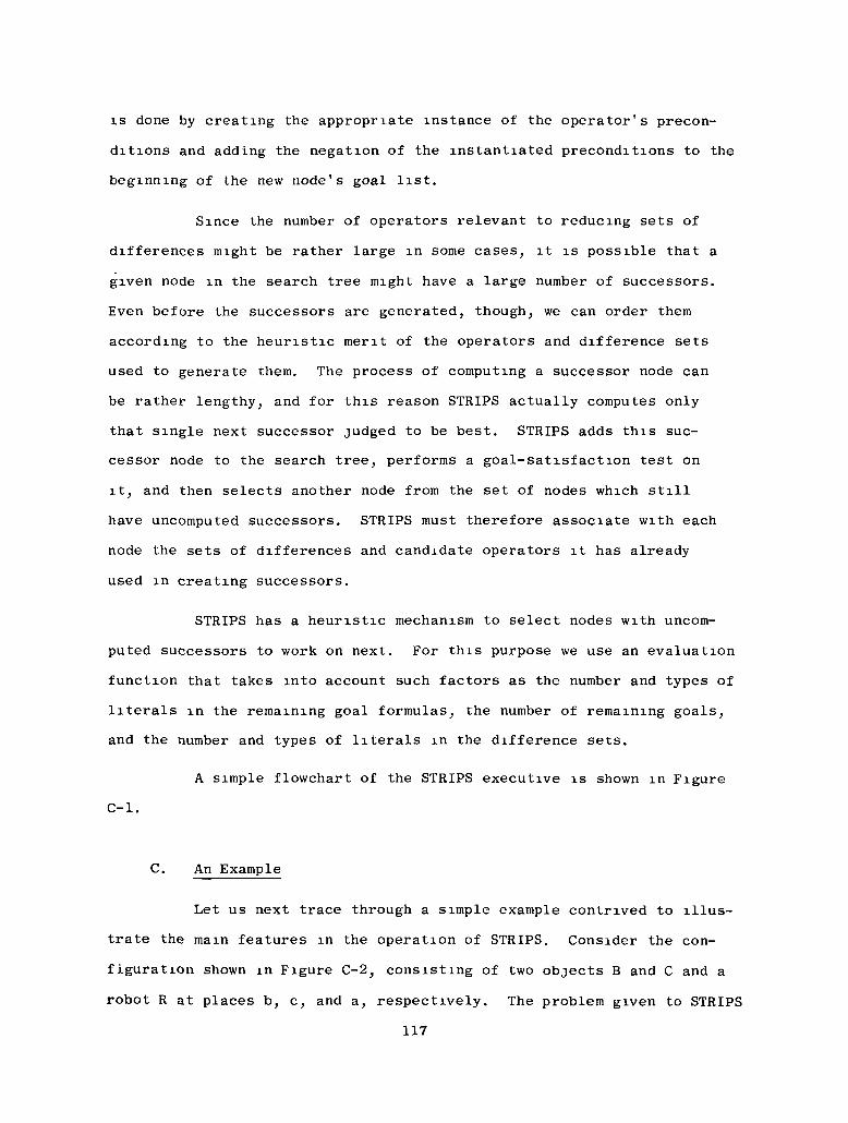
is done by creating the appropriate instance of the operator's precon-
ditions and adding the negation of the instantiated preconditions to the
beginning of the new node's goal list.
Since the number of operators relevant to reducing sets of
differences might be rather large in some cases, it is possible that a
given node in the search tree might have a large number of successors.
Even before the successors are generated, though, we can order them
according to the heuristic merit of the operators and difference sets
used to generate them. The process of computing a successor node can
be rather lengthy, and for this reason STRIPS actually computes only
that single next successor judged to be best. STRIPS adds this suc-
cessor node to the search tree, performs a goal-satisfaction test on
it, and then selects another node from the set of nodes which still
have uncomputed successors. STRIPS must therefore associate with each
node the sets of differences and candidate operators it has already
used in creating successors.
STRIPS has a heuristic mechanism to select nodes with uncom-
puted successors to work on next. For this purpose we use an evaluation
function that takes into account such factors as the number and types of
literals in the remaining goal formulas, the number of remaining goals,
and the number and types of literals in the difference sets.
A simple flowchart of the STRIPS executive is shown in Figure
01.
C. An Example
Let us next trace through a simple example contrived to illus-
trate the main features in the operation of STRIPS. Consider the con-
figuration shown in Figure C-2, consisting of two objects B and C and a
robot R at places b, c, and a, respectively. The problem given to STRIPS
117

01
IDX
<rCO
trO
cc<o
O
ccD
118

ROBOT
TA-8259-31
FIGURE C-2 CONFIGURATION OF OBJECTS AND ROBOT FOR EXAMPLE PROBLEM
is to achieve a configuration in which object B is at place k and in
which object C is not at place c.
The existentially quantified theorem representing this problem
can be written
(3s)[AT(B,k,s) A~AT(C,c,s)]
If we can find an instance of s (in terms of a composition of operator
applications) that satisfies this theorem, then we will have solved the
problem. The negation of the theorem is
G : ~AT(B,k.s) V AT(C.c.s)o
119

Let us suppose that STRIPS is to compose a solution using the
two operators goto and push. These operators can be described as
follows:
(1) push(u,x,y): Robot pushes object u from place x
to place y.
Precondition formula:
(3u,x,s)[AT(u,x;s) AATR(x,s)]
Negated precondition formula:
~AT(u,x,s) V ~ATR(x,s)
Delete list:
AT(u,x,s)
ATR(x,s)
Add list:
/ *AT(u,y,push (u,
/ *ATR(y,push (u,
*where s is the state to which the operator is
applied.
(2) goto(x,y)• Robot goes from place x to place y.
Precondition formula:
120

(3x,s)ATR(x,s)
Negated precondition formula:
~ATR(x,s)
Delete list:
ATR(x,s)
Add list:
/ *ATR(y,goto (x,y,s
The initial configuration can be described by the following
world model:
s : ATR(a.s )o o
AT(B,b,s
AT(C,c,SQ)
In addition, we have a universal formula, true in all world models, that
states if an object is in one place, then it is not in a different place:
F: (Vu,x,y,s)[AT(u,x,s) A (x y) =>~AT(u,y, s)]
The clause forir of this formula is
121

F': ^AT(u,x,s) V (x=y)
We assume that F' is adjoined to all world models.
A portion of STRIPS' solution trace relating to the final plan
is given in Figure C-3. The remainder of this section is a commentary on
that trace. STRIPS first constructs the node N , consisting of the list
(s ,(G )). as the root of the problem-solving tree and tests it for ao o
solution by attempting to find a contradiction for the set s U [G }.
No contradiction is found but some resolvents can be obtained; among
them is the resolvent R of G and F':1 o
~AT(B,k,s) V (c=y) V ~AT(C,y,s)
Next STRIPS selects a node (N is now the only one available)o
and begins to generate successors. First it selects a difference set
D from the set of resolvents attached to N . In this case it sets1 o
D = [R }. Then STRIPS composes a list L of candidate operators for
reducing D . Here L would consist of the single element push.
Next STRIPS attempts to reduce D using clauses on the add
list of push. Again using theorem-proving methods we obtain two re-
*solvents from D and AT(u,y,push (u,x,y,s ):
and
~AT(B,k,push'(C,x,y,s )) V (c=y)
jpush'CBjXjk^s )) V (c=y)
Assuming that these resolutions represent acceptable reductions in the
difference, we extract the state terms of the resolvents to yield
122

Begin STRIPS trace
Create negated goal G : ~AT(B,k,s) V AT(C,c,s)o
Form model s : ATR(a.s )o ' o
ATCB.b.s )o
AT(C.c.s )' o
~AT(u,x,s) V (x=y) V ~-AT(u,y,s)
Form node N : (s .(G ))o o o
Perform goal satisfaction test on node N
Goal G not satisfied; resolvents formed:o
R : ~AT(B,k,s) V (c=y) V~AT(C,y,s)
R2: ...
Select node No
Compute offspring node of No
Create difference D : {R }
Create candidate operators list L : (push)
Test relevancy of push
Relevant instances of push found:
OP : push(C,x,y)
OP : push(B,x,k)iL _ _
Create negated goal G : ~AT(C,x,s) V ~ATR(x,s)
Create node N : (s ,(G .G ))
Perform goal satisfaction test on node N
Goal G not satisfied; resolvents formed:
R':*J
»;=
FIGURE C-3 SOLUTION TRACE FOR EXAMPLE PROBLEM
123
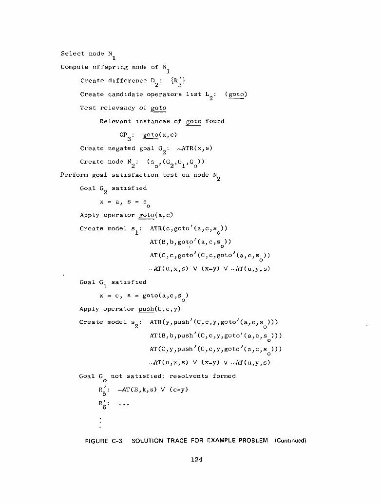
Select node N
Compute offspring node of N
Create difference D : [n'}
Create candidate operators list L : (goto)
Test relevancy of goto
Relevant instances of goto found
OP : goto(x,c)O
Create negated goal G : ~ATR(x,s)£1
Create node N : (s , (G ,G ,G ))£i O ^ J. O
Perform goal satisfaction test on node N
Goal G satisfied£i
x = a, s = s' o
Apply operator goto(a, c)
Create model s : ATR(c,goto ' (a,c,s ))
AT(B,b,goto ' (a ,c ,s ) )
~AT(u,x,s) V (x=y) V ~AT(u,y,s)
Goal G satisfied
x = c, s = goto(a,c,s )
Apply operator push(C, c, y)
ATR(y_,pu
AT(B,b,push'(C,c,y,goto'(a,c,s
ATCC^y^push'CC^c^y^g
~AT(u,x,s) V (x=y) V
ied; resol
R': AT(B,k,s) V (c=y)
Create model s : ATR(y_,push' (C,c^y, goto'(a^c^ s )))2 o
)))o
)))
Goal G not satisfied; resolvents formedo
FIGURE C-3 SOLUTION TRACE FOR EXAMPLE PROBLEM (Continued)
124

Select node N
Compute offspring node of N
Create difference D : [R'}o o
Create candidate operators list L • (push)3
etc.
FIGURE C-3 SOLUTION TRACE FOR EXAMPLE PROBLEM (Concluded)
appropriate instances of the relevant operator. This gives us:
OP : push(C,x,y)
and
OP : push(B,x,k)£i ~~~""—
For brevity, let us consider just OP and construct G , the
negated version of the precondition formula for OP :
G : ~AT(C.,x.,s) V ~ATR(x,s)
This formula is then used to construct a successor node
Y (V(VG0})
STRIPS then performs a goal test on N by attempting to find a contra-
diction for s U G .o 1
Again no contradiction is found, but the following resolvents
are obtained:
125

R : ~ATR(c.s ) from G and AT(C.c.s )3 o 1 ' ' o
and
R : ~AT(C,a,s ) from G and ATR(a.s )4 o 1 o
Although these clauses represent differences between s and G , we do
not insist that these differences be reduced in s . We would accept ao
reduction occurring in any w.orld model, so STRIPS rewrites the clauses
as:
R': ~ATR(c,s)
and
R': ~AT(C.a,s)4
Next STRIPS selects a node for consideration. When it selects
N , it sets the difference set, D , to {R'}.1 ^ O
The list of operators useful for reducing D consists only of£1
goto. STRIPS now attempts to perform resolutions between the clauses
on the add list of goto and D . The clause in D resolves with2 2
ATR(y,goto'(x,y,s )) to yield nil, and answer extraction produces the
instance substituted for the state term, namely
s = goto'(x,c,s )
Thus STRIPS identifies the following instance of goto:
OP : goto(x,c)o
The associated negated precondition is
126

G : ~ATR(x,s)
STRIPS then constructs the successor node
V
and immediately attempts to find a contradiction for s U G . Here ao 2
contradiction is obtained, and answer extraction yields the state term:
goto'(a,,c,s )
Thus STRIPS applies goto(a,c) to s to yieldo
s ATR(c,goto/(aJ)c,s )
AT(B,b,goto'(a,c,s
AT(C,c,goto'(a,c,s ))
Node N is then changed to
<V(Gl'Go)}
and STRIPS immediately checks for a contradiction for s U G . Again a
contradiction is found; answer extraction produces the following in-
stances for x and s:
x = c
and
s = goto'(a,c,s )
127

thetig
itrstOf Op
ls tht
AT(C
fant
(C.
to
*>c.
of the foil

The clause at the root produces one of the resolvents to be attached to
N . namely
R : ~AT(B,k,s) V (c=y)o
When STRIPS selects N , it begins generating successors based£i
on a difference D = [R'}. The operator list for this difference con-«3 O
sists solely of push, and the relevant instance of push is found to be
OP : push(B,x,k)4
Its (negated) precondition is
G : ^AT(B.x.s) V ~ATR(x.s)
A successor node to N is then
V
STRIPS finds a contradiction between s and G , and extracts^ O
s = push'(C,c,b,goto'(a,c,s ))o
and x = b. Therefore, it applies push(B,b,k) to an instance of s2
(with y = b) to yield
s : ATR(k;push/(B,b,k,push'(C,c,b,goto'(a,c,s ))))
O O
AT(B.k,push'(B,b,k,push'(C,c,b,goto'(a,c,s ))))o
AT(C,b,push/(B,b,k,,push/(C,c,b,goto'(a,c.Is ))))
129

Node N is then changed to
_,3
STRIPS can find a contradiction between s and G [assuming that the3 o
equality predicate (b = c) can be evaluated to be false] and exits
successfully. The successful plan is embodied in the state term for s .o
D. Efficient Representation of World Models
A primary design issue in the implementation of a system such
as STRIPS is how to satisfy the storage requirements of a search tree
in which each node may contain a different world model. We would like
to use STRIPS in a robot or quest ion-answering environment where the
initial world model may consist of hundreds of wffs. For such applica-
tions it is infeasible to recopy completely a world model each time a
new model is produced by application of an operator.
We have dealt with this problem in STRIPS by first making the
assumption that most of the wffs in a problem's initial world model will
not be changed by the application of operators. This is certainly true
for the class of robot problems we are currently concerned with. For
these problems most of the wffs in a model describe rooms, walls, doors,
and objects, or specify general properties of the world which are true
in all models. The only wffs that might be changed in this robot environ-
ment are the ones that describe the status of the robot and any objects
which it manipulates.
Given this assumption, we have implemented the following
scheme for handling multiple world models. All the wffs for all world
models are stored in a common memory structure. Associated with each
130

wff (i.e., clause) is a visibility flag, and QA3 has been modified to
consider only clauses from the memory structure which are marked visible.
Hence, we can "define" a particular world model for QA3 by marking that
model's clauses visible and all other clauses invisible. When clauses
are entered into the initial world model they are marked visible and
given a variable as a state term. Clauses not changed will remain
visible throughout STRIPS' search for a solution.
Each world model produced by STRIPS is defined by two clause
lists. The first list, DELETIONS, names all those clauses from the
initial world model which are no longer present in the model being de-
fined. The second list, ADDITIONS, names all those clauses in the model
being defined which are not also in the initial model. These lists
represent the changes in the initial model needed to form the model
being defined, and our assumption implies they will contain only a small
number of clauses.
To specify a given world model to QA3, STRIPS marks visible
the clauses on the model's ADDITIONS list and marks invisible the
clauses on the model's DELETIONS list. When the call to QA3 is com-
pleted, the visibility markings of these clauses are returned to their
previous settings.
When an operator is applied to a world model, the DELETIONS
list of the new world model is a copy of the DELETIONS list of the old
model plus any clauses from the initial model which are deleted by the
operator. The ADDITIONS list of the new model consists of the clauses
from the old model's ADDITIONS list as transformed by the operator plus
the clauses from the operator's add list.
To illustrate this implementation design we list below the
way in which the world models described in the example of the previous
section are represented:
131

s : ATR(a.s)o
AT(B,b,s)
AT(C,c,s)
s ' DELETIONS: ATR(a,s)
ADDITIONS: ATR(c, goto' (a, c, s ))
s • DELETIONS: ATR(a,,s)£t
AT(C,c,s)
ADDITIONS: ATR(y, push' (C, c,y, goto' (a, c , SQ) ) )
s • DELETIONS: ATR(a,,s)J
AT(C,c,s)
AT(B,b,s)
ADDITIONS: ATR(k,push' (B, b , k,push' (C, c,b, goto' (a, c, s ))))
AT (B, k , push ' (B , b,k, push '(C,c,b, goto ' (a,c,S ))))
IV FUTURE PLANS AND PROBLEMS
The current implementation of STRIPS can be extended in several
directions. These extensions will be the subject of much of our problem-
solving research activities in the immediate future. We shall conclude
this note by briefly mentioning some of these.
We have seen that STRIPS constructs a problem-solving tree whose
nodes represent subproblems. In a problem-solving process of this sort,
there must be a mechanism to decide which subproblem to work on next.
132

We have already mentioned some of the factors that might be incorporated
in an evaluation function by which subproblems can be ordered according
to heuristic merit. We expect to devote a good deal of effort to de-
vising and experimenting with various evaluation functions and other
ordering techniques.
Another area for future research concerns synthesis of more complex
procedures than those consisting of simple linear sequences of operators.
Specifically we want to be able to generate procedures involving itera-
tion (or recursion) and conditional branching. In short, we would like
STRIPS to be able to generate computer programs. Several researchers5^9^10
have already considered the problem of automatic program synthesis and
we expect to be able to use some of their ideas in STRIPS.
Our implementation of STRIPS is designed to facilitate the defini-
tion of new operators by the user. Thus the problem-solving power of
STRIPS can gradually increase as its store of operators grows.
An idea that may prove useful in robot applications concerns de-
fining and using operators to which there correspond no execution rou-
tines. That is, STRIPS may be allowed to generate a plan containing
one or more operators that are fictitious. This technique essentially
permits STRIPS to assume that certain subproblems have solutions without
actually knowing how these solutions are to be achieved in terms of
existing robot routines. When the robot system attempts to execute a
fictitious operator, the subproblem it represents must first be solved
(perhaps by STRIPS). (In human problem solving, this strategy is em-
ployed when we say: "l won't worry about that [sub] problem until I
get to it.")
We are also interested in getting STRIPS to define new operators
for itself based on previous problem solutions. One reasonable possi-
bility is that after a problem represented by (S ,(G )) is solved,o o '
133

STRIPS could automatically generate a fictitious operator to represent
the solution. It would be important to try to" generalize any constants
appearing in G ; these would then be represented by parameters in theo
fictitious operator. The structure of the actual solution would also
have to be examined in order to extract a precondition formula, delete
list, and add list for the fictitious operator.
A more ambitious undertaking would be an attempt to synthesize
automatically a robot execution routine corresponding to the new '
operator. Of course, this routine would be composed from a sequence
of the existing routines corresponding to the individual existing
operators used in the problem solution. The major difficulty concerns
generalizing constants to parameters so that the new routine is general
enough to merit saving. Hewitt11 discusses a related problem that he
calls "procedural abstraction." He suggests that from a few instances
of a procedure, a general version can sometimes be synthesized. We ex-
pect that our generalization problem will be aided by an analysis of
the structure of the preconditions and effects of the individual
operators used in the problem solution.
ACKNOWLEDGMENT
The development of the ideas embodied in STRIPS has been the re-
sult of the combined efforts of the present authors, Bertram Raphael,
Thomas Garvey, John Munson, and Richard Waldinger, all members of the
Artificial Intelligence Group at SRI.
134

REFERENCES
1. J. H. Munson, "Robot Planning, Execution, and Monitoring in an
Uncertain Environment," paper submitted for presentation to the
Second International Joint Conference on Artificial Intelligence,London, England, 1-3 September 1971.
2. N. J. Nilsson, Problem-Solving Methods in Artificial Intelligence
(McGraw-Hill Book Company, New York, to appear in April 1971).
3. C. Green, "Theorem Proving by Resolution as a Basis for Question-
Answering Systems," in Machine Intelligence 4, B. Meltzer and
D. Michie (eds.), pp. 183-205 (American Elsevier Publishing Co.,
Inc., New York, 1969).
4. G. Ernst and A. Newell, GPS: A Case Study in Generality and
Problem Solving, ACM Monograph Series (Academic Press, 1969).
5. C. Green, "Application of Theorem Proving to Problem Solving,"Proc. Intl. Joint Conf. on Artificial Intelligence, Washington,
D.C. (May 1969).
6. D. Luckham and N. Nilsson, "Extracting Information from Resolution
Proof Trees," Artificial Intelligence (to appear).
7. J. McCarthy and P. Hayes, "Some Philosophical Problems from the
Standpoint of Artificial Intelligence," in Machine Intelligence 4,
B. Meltzer and D. Michie (eds.), pp. 463-502 (American Elsevier
Publishing Co., Inc., New York, 1969).
8. B. Raphael, "The Frame Problem in Problem-Solving Systems," Proc.
Adv. Study Inst. on Artificial Intelligence and Heuristic
Programming, Menaggio, Italy (August 1970).
9. R. Waldinger and R. Lee, "PROW: A Step Toward Automatic Program
Writing," Proc. Intl. Joint Conf. on Artificial Intelligence,
Washington, D.C. (May 1969).
135

10. Z. Manna and R. Waldinger, "Toward Automatic Program Synthesis/'
Artificial Intelligence Group Technical Note 34, Stanford Research
Institute, Menlo Park, California (July 1970).
11. C. Hewitt, "Planner: A Language for Manipulating Models and
proving Theorems in a Robot," Artificial Intelligence Memo No. 168
(Revised), Massachusetts Institute of Technology, Project MAC,
Cambridge, Massachusetts (August 1970).
136

Appendix D
A LANGUAGE FOR WRITING PROBLEM-SOLVING PROGRAMS
by
Johns F. Rulifson, Richard J. Waldinger and Jan A. Derksen
137
Appendix D
A LANGUAGE FOR WRITING PROBLEM-SOLVING PROGRAMS
ABSTRACT
This appendix describes a language for constructing problem-solving
programs. The language can manipulate several data structures, in-
cluding ordered and unordered sets. Pattern matching facilities may
be used in various ways, including the binding of variables. Implicit
backtracking facilitates the compact representation of search procedures.
Expressions are treated analogously to atoms in LISP. A "context" de-
vice is used to implement variable bindings, to effect conditional
proofs, and to solve the "frame" problem in robot planning.
I BACKGROUND
In order to design a deductive problem-solving program, we are
constructing a new formal language that can express complex inferential
mechanisms concisely. This language, called the QA4 language, is being
used to build a proposed intelligent system, called the QA4 system, that
will be able to organize and use a large body of specialized knowledge.
The selection of three specific applications--automatic program synthesis,
automaton planning, and theorem proving—permits a concentration of effort
within a framework of generality. All three applications, however, share
a common basis that encompasses natural language dialogue, question
answering, and inference, as well as many other areas of Artificial
Intelligence.
139

There is strong motivation for the development of a new language
for problem-solving programs. Earlier systems have been constrained
by fixed inference mechanisms, built-in strategies, awkward languages
for problem statement, and rigid overall structure. They relied on one
or two rules of inference that could not be changed. To modify a
strategy required a complete reprogramming of the system. It was some-
times harder to express a program-synthesis problem in a language the
system could understand than it was to write the program yourself.
Systems were limited to the use of a single paradigm that might be
applicable to some types of problems and inappropriate for others.
Theorem-proving strategies have used syntactic properties of the ex-
pressions being manipulated, but have been unable to use semantic
knowledge or pragmatic, intuitive information. They have been unable
to employ the sort of pattern recognition the human problem solver re-
lies on so heavily.
The basic approach of the QA4 project is to develop natural, in-
tuitive representations of specific problems and their solutions. The
specification for a computer program, for example, is a blend of pro-
cedural and declarative information that includes explicit instructions,
intuitive advice, and semantic definitions. A QA4 interpreter will
execute programs in the transparent but precise language we have chosen
for these representations; and the interpreter, together with an initial
collection of QA4 "bootstrapping" programs, will constitute the basic
QA4 system. The system will attempt to assimilate new advice and facts
and attempt to solve problems with continually increasing agility.
The project has revolved around the construction and reworking of
hand simulations of a proposed final QA4 system. Each simulation in-
cludes a problem statement, relevant definitions and advice, and a
protocol for the solution. These simulations have provided a focus
140

for the language development and prompted explorations into theoretical
foundations of the problem areas.1 Table D-l summarizes the scope of
the simulations and indicates the problem areas attacked.
Table D-l
PROBLEM AREAS
Program Synthesis
• Generate recursive and iterative programs from declarative
axiomatic specifications (problems taken from a LISP primer).
• Generate an iterative program from a recursive procedural
definition (see Fibonacci example in Ref. 2).
• Verify the correctness of programs with respect to input/output
relations. These relations may be defined in terms of
executable programs, as well as in terms of declarative axioms.
Automaton Planning
• Generate plans for simple robot problems.
Theorem Proving
• Prove simple algebraic identities over the integers.
• Derive simple algebraic laws from Peano's axioms.
• Prove properties of axiomatically defined groups.
• Accommodate general rules of inference, applicable to any
logical system.
The QA4 language is derived from more conventional programming
languages and mathematical languages, and yet differs from both in many
ways. The basic data structures include sets, sets with repeated ele-
ments ("bags"), ordered bags ("tuples"), and lambda expressions. Data
*References are listed at the end of this appendix.
141

may also be represented implicitly; for example, the set of even integers,
although infinite, may still be described and manipulated in the system.
Every expression in the language may have a variety of properties asso-
ciated with it. This feature serves as the basis for describing the
role of each expression and thus directing the processes that operate
on the expression. Program control is often directed by matching pat-
terns against expressions. Sometimes, for example, the syntactic form
of a problem suggests the use of a certain strategy. Ambiguous patterns
lead to nondeterministic programs and the need for automatic back-
tracking.3 Other control features include parallel search and iteration
through sets. Space does not permit a full presentation of our current,
preliminary version of the QA4 syntax. Table D-2 lists some features
of the language.
The system changes continuously as it is used. The programmer types
commands in the form of QA4 expressions to a top-level function. The
commands may input or modify expressions or properties of expressions;
define, modify, or execute programs; or perform debugging tasks.
The input system of QA4 is a parser that transforms QA4 infix ex-
pressions into internal prefix format. The parser uses the input trans-
later BIP,4 and has the advantage of being readily modified. Similarly,
an output function takes the internal expression form and produces a
corresponding infix output stream. Thus the user always communicates
with QA4 in an infix mathematical-style notation.
The QA4 interpreter is a function resembling LISP EVAL.5 It accepts
QA4 expressions and, with the aid of an extensive library of primitive
functions, executes them.- Unlike LISP programs, QA4 expressions may
succeed or fail and do not necessarily have values. The interpreter
performs its task in small steps, and may, between any two steps, re-
direct its attention to other parallel processes or search programs.
142

Table D-2
SOME LANGUAGE FEATURES
Data Manipulation
• Arithmetic and Boolean operations
• Set, bag, and tuple operations
• Expression decomposition and construction
Pattern Matching
• Actual argument decomposition
• Data base queries
• Monitoring expression properties
• Invoking of strategies and inference rules
Control
• Standard serial and conditional statements
(prog's, labels, go's, and if's)
• Iterative forms for sets, bags, and tuples
• Automatic backtracking
• Strategy controlled parallel interpretation
II DATA CONTROL STRUCTURES
Every operator in QA4 has a single operand. The data type of each
primitive operator has been chosen to eliminate a proliferation of
rules governing algebraic properties, such as associativity, commuta-
tivity, and transitivity. The Boolean connective "and," for example,
has a set as its operand. The finix expression A & B & C is translated
into the internal representation AND^A, B, C] (where braces denote the
data type ''set''). Since sets are independent of the order of their
elements, this representation makes the statement of the commutativity
law unnecessary.
143

Bags in QA4 are unordered tuples or, equivalently, sets with re-
peated elements. They play an important role in the definition of
arithmetic operators, such as addition. The operand of PLUS cannot be
a set, because the set [l, 1} is equal to {l}, but we would not want
PLUS{1, 1} to equal PLUS{l}. .Instead, the infix expression X + Y + Z
becomes PLUS[X, Y, Z] internally, where [X, Y, Z] is a bag. Bags are
evaluated by first evaluating their members. The resulting values are
collected together into a bag, elements being duplicated when appro-
priate. Thus, if X, Y, and Z all had value 1, our expression would
equal PLUS[1, 1, 1], and its value would be 3.
Some expressions, infinite sets, for example, cannot always be ex-
plicitly evaluated. Finite sets may also be inconvenient to evaluate:
A program may wish to search the Cartesian product of two sets, even
when the entire set is too large to generate. The interpreter can per-
form the search by indexing through the original two sets. In cases
such as this expressions are said to have implicit values.
QA4 has iterative, parallel, and backtracking control structures.
The iterative statement forms of the language operate over sets, bags,
and tuples. The order of iteration may be controlled by relations.
During theorem proving experiments, for example, pairs of logical ex-
pressions are analyzed in an order specified both in terms of syntactic
properties, such as length, and of pragmatic properties, such as fre-
quency of use. Parallel structures, in the form of coroutines and WHEN
statements, are used in the construction of problem solving strategies.
For example, in order to prove a theorem of the form A V B, we may wish
to establish two processes, one to prove A and the other to prove B. If
either terminates successfully, the proof is complete. Nondeterministic
programs give rise to backtracking. If a point of indeterminacy occurs,
a choice determined by a prespecified strategy is made. If the program
144

later fails, control is reestablished at the choice point, and a dif-
ferent selection is made.
Without explaining all the notations we use, we illustrate the
power of the QA4 language with a program that sorts bags:
SORT = CASES
U t ], < >,
X X-B T MIN(X,B>, X-SORT(B));
When this function is applied to a bag, say B', it first checks to see
whether B is empty ([ ]); if so, it returns the empty tuple (( )). If
the bag is not empty, it finds an element X of B' such that X is less
than or equal to all the elements of B, the bag remaining when X is de-
leted from B'. Then it sorts B (recursively) and adjoins X to the front
of the resulting tuple. Thus the bound variables of a lambda expression
may be patterns, and variable binding must then be done by pattern
matching. The search for a pattern match may be directed by an associated
strategy.
Ill EXPRESSIONS
The data base for QA4 programs is made up of QA4 expressions. An
expression is represented internally by a list of properties, one of
which is the syntactic component that uniquely distinguishes it from all
other QA4 expressions. This list stores arbitrary properties, and each
property is, in turn, a QA4 expression. These properties fall into three
categories: syntactic, semantic, and pragmatic. Table D-3 is a brief
example of an expression. Table D-4 lists commonly used properties
145

Table D-3
A SAMPLE EXPRESSION
Syntactic component
Value
Length
Result when the function
F is applied to the expression
, 4)
27
Table D-4
EXPRESSION PROPERTIES
Syntactic
• The form
The logical type (e.g., a function mapping numbers into truthvalues)
The data type (e.g., a set of 3-tuples)
Frequently used information (e .g. , the length)
Semantic
The value
An implicit value (e.g., a coroutine6 that generates the value)
A set of expressions equal to this one
Constraints (e.g., a range or interval for the value)
Pragmatic
Historical information
Intuitive evaluation advice
Success/failure indicators
146

Expression manipulation is accomplished by decomposition and con-
struction. In QA4 decomposition means naming parts or components of an
expression. The naming is done by the pattern matcher. Patterns may
occur at many points in the language: in formal arguments of functions,
in assignment statements, and in conditional tests. Table D-5 illustrates
some of the more useful facets of the pattern matching notation. Trans-
formation of expressions is done through a complete set of constructors,7
such as: add an element to a set, add onto tuples, or construct a lambda
expression.
Table D-5
SOME PATTERN MATCHER FEATURES
Transparent template notation
Matching of internal or external
notation
Fragment variables
Type constraints on variables
Predicate constraints
"Occurs in" matching
(X,4,3> matches (5,4,3)with X = 5
(X,4) matches (tuple 3 4)with X = 3
(2, * Y) matches (2,3,4,5)
with Y = (3,4,5)
X/integer matches 3with X = 3
(X T X s 4,5,6) does not
match (2,5,6)
•• + •• matches A * 2 + B
Given the syntactic component for an expression, a fundamental
operation is to retrieve the entire expression so as to find the proper-
ties already assigned or known about it. In this way, LISP's atom
property feature is extended to expressions in general. When an expres-
sion is stored, whether the expression has been stored before is deter-
mined. If it has been, the old expression is returned; if not, the new
expression is retained by the system.
147

The storage mechanism is a discrimination net. Each node of the
net consists of a feature selector and a set of labeled branches. A
syntactic component is retrieved by applying the topmost selector,
choosing a branch based on the outcome of the selector, and repeating
the process until either a terminal node is reached or there is no
appropriate branch. When conflicts occur at a terminal node, a new
selector is automatically generated and installed at the new node. The
next time the same syntactic component is retrieved, the expression that
has just been added will be returned. The net also serves as a pruning
device for the pattern matcher.
If two QA4 expressions are identical except for the names of their
bound variables, they have the same internal representation. Thus bound
variables are not used as discrimination features. Moreover, in order
to store sets and bags in the net, an index is assigned to each element
of a set or bag expression the first time the expression is stored. If
the same set is then stored a second time (perhaps with some elements
permuted), the elements are first ordered by their index numbers and
then discriminated upon syntactically. If a user types in the set
[A, B, C], the elements might be assigned indices A«-l, B*-2, C«-3. If
the set [C, B, A] is entered, it is sorted into {A, B, C] and then
found to occur already. The storage and retrieval functions also main-
tain extensive statistics concerning the number of references made to
each expression for use in future optimization.
Variable bindings are implemented in the QA4 interpreter with a
"context" mechanism—a method of storing all the changeable properties
of expressions which simplifies backtracking and executing parallel
processes. The same facilities, moreover, are made available to users
and are especially useful in programs dealing with conditional proofs
or robot planning programs confronted with the "frame" problem.8
148

IV CONCLUSION
Certain structures and mechanisms have found repeated application
in deductive problem solvers. It is our goal to give these concepts
concise notations. We expect this effort to have several desirable
consequences'
• Existing problem-solving techniques should become more
easily representable and modifiable.
• A large store of special-purpose knowledge could be
embodied in a program.
• Systems would be more likely to rely on strategies than
on blind search if such strategies were easily expressed
and incorporated.
We have found the QA4 language a suitable vehicle for our own work in
program synthesis, robot planning, and theorem proving.
V ACKNOWLEDGMENT
The development and use of the QA4 system has been supported at
Stanford Research Institute by the Advanced Projects Research Agency
and the National Aeronautics and Space Administration (NASA) under
Contract NAS12-2221, by NASA under Contract NASW-2086, and by Air Force
Cambridge Research Laboratories under Contract F19628-70-C-0246.
149

REFERENCES
1. Z. Manna and R. Waldinger, "Towards Automatic Program Synthesis,"
Artificial Intelligence Group Technical Note 34, Stanford Research
Institute, Menlo Park, California (July 1970). [Submitted for
publication in Collection of Lecture Notes in the Symposium on theSemantics of Algorithmic Languages, Erwin Engeler (ed.), Springer
Verlag.] [Also submitted for publication in the CACM.]
2. J. F. Rulifson, R. J. Waldinger, and J. Derksen, "QA4 Working
Paper," Artificial Intelligence Group Technical Note 42, Stanford
Research Institute, Menlo Park, California (October 1970).
3. L. Golomb and L. Baumert, "Backtrack Programming," J. ACM, Vol. 12,
No. 4, pp. 516-524 (October 1965).
4. R. E. Fikes, "A LISP Implementation of BIP," Artificial Intelligence
Group Technical Note 22, Stanford Research Institute, Menlo Park,
California (February 1970).
5. J. McCarthy et al., LISP 1.5 Programmer's Manual (M.I.T. Press,Cambridge, Massachusetts, 1962).
6. M. E. Conway, "Design of a Separable Transition-Diagram Compiler,"CACM, Vol. 6, pp. 396-408 (1963).
7. P. J. Landin, "The Mechanical Evaluation of Expressions," ComputerJ_._, Vol. 6, pp. 308-320 (1963-64).
8. J. McCarthy and P. Hayes, "Some Philosophical Problems from the
Standpoint of AI," in Machine Intelligence 4, B. Meltzer and
D. Michie (eds.) (Edinburgh University Press, Edinburgh, Scotland,1969).
150

Appendix E
FAILURE TESTS AND GOALS IN PLANS
by
Richard E. Fikes
151

Appendix E
FAILURE TESTS AND GOALS IN PLANS
I INTRODUCTION
This appendix describes a proposal for the form that plans for the
Stanford Research Institute mobile automaton might take and the rules
an interpreter might use to execute these plans. We are particularly
concerned here with adding tests to a plan that allow the executor to
determine whether execution of a plan is succeeding and that specify
what is to be done when a failure occurs.
We proceed by developing a syntax and semantics for plans in the
i *context of STRIPS (STanford Research Institute Problem Solver), the
program that acts as a planner for the automaton system. Subsequently,
we present an algorithm that STRIPS can use to create the tests for the
executor to use.
We assume that the reader has some familiarity with the capabilities
of our robot vehicle and our means of modeling both the robot's external
environment and its action routines (or operators). See Refs. 1 and 2
for this background material.
II SYNTAX AND SEMANTICS OF A STRIPS PLAN
The role of the planner in our system is to determine what the
robot should do to solve a given task. We may consider the output of
*References are listed at the end of this appendix.
153

the planner to be a program each of whose steps is an operator to be
executed or a test to be made on the world model. One simple form that
a plan might have is the following:
BEGIN
DO operator ,
GOAL preconditions for operator ;
DO operator ,
^GOAL preconditions for operator ;
GOAL preconditions for operator ;k
DO operator ,K
GOAL task statement
END.
The executor of the plan will call the operator routines contained in
the DO statements and will employ a theorem prover such as QA3.53;4
(a resolution-based deductive system) to determine whether the predi-
cates contained in the GOAL statements are true in the world model at
each step.
The GOAL statements in a plan provide a means of testing whether^
execution of the plan is proceeding successfully. We^assign to the
planner the responsibility of generating the information needed for
these tests. In the form for a plan given above this information is
merely the GOAL statements that determine whether the next operator in
the plan can be applied, and a final GOAL statement to determine whether
the task has been completed.
We would like the planner to provide statements in the plan that
will allow the executor to determine as soon as possible when execution
of the plan is failing. For example, if the success of some operator
154

in a plan depends on a box Bl being at some location LA and a side
effect of execution of some earlier operator in the plan is the de-
termination that Bl is not located at LA, then we would like the plan
to contain statements that would allow the executor to realize that the
new location of Bl is going to cause an eventual failure. Execution
of the plan could then be discontinued without incurring the costs of
doing the operations that precede the point in the plan where the actual
failure would occur.
To see how STRIPS provides this type of information in its plans,
we first note that it employs a means-ends analysis search strategy
similar to that of GPS5 to grow a search tree whose nodes specify world
models and some of whose arcs represent planned operator applications.
The means-ends analysis strategy directs search by creating subgoals
and determining relevant operators. The theorem prover, QA3.5, is used
to ask questions about world models, such as whether a goal is true in
a model or whether an operator's preconditions are true in a model. A
complete description of STRIPS can be found in Ref. 1.
STRIPS can create a plan when there is a path through its search
tree of the following form:
operator operator operator
where S is the initial world model, each S is the world model that
would be produced by applying operator to model S } and S is the
model in which the task statement is satisfied. The operators on this
path define the DO statements for the plan; each operator's precondi-
tions and the task statement define the plaVs GOAL statements.
STRIPS forms additional tests for the plan by extracting informa-
tion from the proofs produced by QA3.5. For the search-tree path we
155

are considering, QA3.5 will have been used to prove that the task state-
ment is true in S , and that the preconditions for each operator arek i
true in S . For each of these proofs, STRIPS determines which axioms
from the world model were used. Any of these axioms from a given model
that were not added to the model as one of the effects of the previous
operator in the plan must also have been in the model before that operator
was executed. This implies that STRIPS can add a test to the plan be-
fore the DO statement for that operator that will prevent the DO state-
ment' s execution if one of these axioms is missing from the model. This
process can be iterated backwards through the plan so that tests can be
inserted before each DO statement indicating what axioms the remainder
of the plan assumes exist in the model at that point. Figure E-l shows
an example plan into which test indicators have been inserted.
To include these new tests in the plan, we first surround each DO
statement and the preceding preconditions GOAL statement by a labeled
BEGIN statement and an END statement to form ALGOL-like blocks as follows:
BEGIN
B1:BEGINGOAL preconditions for operator ,
DO operator
END;
B2:BEGIN
GOAL preconditions for operator ;
DO operator
END;
B :BEGINkGOAL preconditions for operator ;
DO operatork
END;
GOAL task statement
END
156

BEGIN
END
(Test for Al)
(Test for A2 and A4)
(Test for A6)
(Test for A7 and A3)
GOAL preconditions for op ,
DO op
(Test for Al)
(Test for A6)
(Test for A7 and A3)
GOAL preconditions for op ,
DO op2
(Test for Al and A12)(Test for A7 and A3)GOAL preconditions for op ,
DO op
(Proof used axioms A8 and A5)
(Adds axiom A9)
(Test for Al and A12)
GOAL
DO op
GOAL preconditions for op ;
GOAL task statement
(Proof used axioms A9, A2, and A4)
(Adds axioms A12 and A10)
(Proof used axioms A10 and A6)
(Adds axiom All)
(Proof used axioms All, A7, and A3)(Adds axioms A10 and A13)
(Proof used axioms Al, A12, and A13)
FIGURE E-1 ABSTRACT PLAN INDICATING POSSIBLE TESTS
Each new test in the plan is represented by a FAILTEST statement
having the following form-
FAILTEST A A A A ... A A FOR B ,B ....,B12 n j' J+1' ' m
where each A is an axiom used by QA3.5 in a proof and each B is the
label of a BEGIN statement in the plan. When the executor encounters
a FAILTEST statement it attempts to determine whether the conjunction
of axioms is true in the current state. If the proof attempt succeeds,
157

then execution continues with the next statement in the plan; if the
proof attempt fails, then those blocks which begin with the labels
listed in the right side of the FAILTEST statement are deleted from the
plan before execution continues.
When deletions occur during the execution of a FAILTEST statement,
the plan is no longer complete and its execution will almost certainly
fail to satisfy some GOAL statement remaining in the plan. When the
executor encounters an unsatisfied GOAL statement, it can recall the
planner to create a plan that will achieve the unsatisfied goal. If
the planner successfully produces such a plan, then the new plan can be
executed to "get back onto the track" of the original plan. If the
planner fails and the goal is.the task-statement goal, then the system
cannot accomplish the task. If the planner fails with any other goal,
then the executor may still be able to retain some of the original plan*
by continuing execution at the next block.
To determine which blocks should be listed in a FAILTEST statement,
the planner assumes that if some axiom that it intends to be true at
some point in a plan is not true at that point when the plan is being
executed, then any proof in which that axiom participated is invalid.
This assumption implies that the FAILTEST statement at that point in
the pl-an can indicate deletion of "any block whose only function in the
plan is to add axioms used in the invalidated proofs.
Figure E-2 shows an instantiation of the example plan from Figure E-l
in the form that STRIPS would produce it. The task for the instantiated
plan is to push the three boxes BOX1, BOX2, and BOX3 to the same location.
*At this point execution of the plan is in deep trouble, and in most
cases FAILTEST statements will be encountered that will cause deletion
of the remainder of the plan.
158

BEGIN
B1:BEGINFAILTEST AT(BOX1,LA) FOR B1,B2,B3,B4;
FAILTEST AT(BOX2,LB)ASAMEROOM(LB,LA) FOR Bl,
IF AT(ROBOT,LD)ASAMEROOM(LD,LB) THEN DO GO(LD,LB)
ELSE GOAL AT ( ROBOT .,LB)
END;B2:BEGIN ,
FAILTEST AT(BOX1,LA) FOR B2,B3,B4;IF AT(ROBOT,LB)AAT(BOX2,LB)ASAMEROOM(LB,LA) THEN DO PUSH(BOX2,LB,LA)
ELSE GOAL AT(ROBOT.,LA)AAT(BOX2, LA)
END;B3:BEGIN
FAILTEST AT(BOX1,LA)AAT(BOX2,LA) FOR B3,B4;FAILTEST AT(BOX3,LC)ASAMEROOM(LC,LA) FOR B3,IF AT(ROBOT,LA)ASAMEROOM(LA,LC) THEN DO GO(LA,LC)
ELSE GOAL AT(ROBOT,LC)END,
B4:BEGIN
FAILTEST AT(BOX1,LA)AAT(BOX2,LA) FOR B4;
IF AT(ROBOT,LC)AAT(BOX3,LC)ASAMEROOM(LC,,LA) THEN DO PUSH(BOX3,LC,LA)
ELSE GOAL AT(BOX3,LA)
END;GOAL (Ex)(AT(BOX1,x)AAT(BOX2,x)AAT(BOX3,x))
END
FIGURE E-2 PLAN FOR THE THREE BOXES PROBLEM
The GO(x,y) operator used in the plan moves the robot from location x to
location y where x and y are constrained to be in the same room. The
PUSH(b;x,y) operator in the plan causes the robot to push an object b
from location x to location y, where both the robot and the object are
assumed to begin at location x.
Note that in the Figure E-2 plan each pair of statements
GOAL preconditions for opi
DO op
has been replaced by an IF statement. STRIPS produces these IF state-
ments in the following form:
159

IF preconditions for op THEN DO opi i
ELSE GOAL relevant results of op ,
where the relevant results of an operator are those axioms added by the
operator that were used during the creation of the plan in the proof of
some subsequent operator's preconditions or the task-statement goal.
Hence the IF statement indicates to the executor that if the operator
can be applied then it should be, otherwise a new plan should be found
and executed that will produce the same results that the operator was to
achieve. For example, in the Figure E-2 plan if the robot is not initially
at location LD, then GO(LD,LB) will not be applied; instead a new plan
will be created to move the robot to location LB, since that was the de-
sired result of applying GO(LD,LB). Also, consider the case where the
robot is at LD initially so that GO(LD,LB) is applied; if GO(LD,LB)
fails to move the robot to LB, then the preconditions for PUSH(BOX2,LB,LA)
will not be satisfied in block B2 and a new plan will be created to
achieve the desired results of pushing BOX2 to LA.
Note also in Figure E-2 the implications of the assumption that a
single missing axiom invalidates any proofs in which the axiom partici-
pated. This assumption causes the first FAILTEST statement in the plan
to indicate deletion of the entire plan if BOX1 is not at location LA.
One might-argue that when a partrcular axiom is not true as expected an
attempt should be made to generate and execute a plan that would make
the axiom true so that the original plan could still be used. That
strategy can easily lead to nonoptimal plans. For example, if BOX1 is
not initially at LA during execution of the plan for the three boxes
problem, then this strategy would dictate that a new plan be constructed
and executed to move BOX1 to LA; once this was accomplished, the original
plan could be executed. This solution of the problem would require
moving all three boxes to a new location; the strategy proposed here of
160

deleting the entire original plan would cause creation and execution of
a new plan involving the movement of two boxes to the third. Hence,
this strategy prefers to expend greater replanning effort so that the
resulting plan will require less execution effort.
Finally, note that some of the tests indicated in the Figure E-l
plan have disappeared in the Figure E-2 plan. The deleted tests were de-
termined by STRIPS to be redundant. For example, a FAILTEST statement
could have been inserted in block Bl to assure that BOX3 was at location
LC; but since failure of that test would cause only block B3 to be de-
leted from the plan, the test need not be made in any of the blocks pre-
ceding block B3.
Ill THE STRIPS ALGORITHM FOR ADDING TESTS TO A PLAN
In this section we present and illustrate an algorithm for creating
the FAILTEST statements and IF statements for a STRIPS plan. The input
to the algorithm is a plan consisting of a sequence of blocks followed
by a GOAL statement containing the task statement. Each block in the
input plan has the following form:
Bi:BEGIN
GOAL preconditions for operator ,
DO operatori
END
The algorithm also knows which axioms were used to prove each operator's
preconditions and the task statement while the plan was being created by
STRIPS. Finally, the algorithm knows from the operator descriptions the
axioms added to the world model by each operator in the plan.
The algorithm is as follows:
1. For each GOAL statement in the plan do the following
procedure:
161

1.1 Create an axiom list, AXL, consisting of the
axioms used by QA3.5 in the goal's proof
during the creation of the plan.
1.2 Proceed backwards through the plan from the
GOAL statement to the initial BEGIN and exe-
cute the following procedure at each DO
statement encountered:
1.2.1 Determine whether the DO state-
ment' s operator added to the
model any of the axioms on the
list, AXL. If it did not, then
take no action at this DO state-
ment. If it did, then continue
at the next step.
1.2.2 Delete from AXL those axioms
added to the model by the
operator and store at the DO
statement a list of the deleted
axioms.
1.2.3 Mark the block in which the DO
statement occurs as being rele-
vant to the goal under con-
sideration by storing at the
block the goal and a copy of
the list, AXL.
2. For each GOAL statement in the plan, do the following
procedure:
2.1 Create a null goal list, GL.
2.2 Create a null block list, BL.
2.3 Proceed backwards through the plan from the
GOAL statement to the initial BEGIN and exe-
cute the following procedure at each block
encountered:
162

2.3.1 Determine whether the block is
marked as being relevant to thegoal under consideration. If
it is then continue at the nextstep. If it is not, then con-
tinue at step 2.3.3.
2.3.2 Set AXL to be the list of axioms
stored at the block with thegoal under consideration.
2.3.3 Determine whether the block is
marked relevant to any goal thatis either not on the list GL or
is not the goal under considera-tion. If it is, then take nofurther action at this block.If it is not, then continue atthe next step.
2.3.4 If there is a GOAL statement in
the block under consideration,
then add the goal to the list GL.
2.3.5 Add the block under consideration
to the list BL.
2.3.6 Insert a FAILTEST statement at thebeginning of the block under con-
sideration to test for the conjunc-tion of the axioms on AXL and todelete the blocks on list BL.
3. For each block on the plan, do the following procedure:
3.1 Form a wff, RELRESULTS, by conjoining all the axiomsstored at the block's operator (in step 1.2.2 of the
algorithm).
3.2 Replace the statements
GOAL preconditions for op ,i
DO operatori
163

in the block by the statement
IF preconditions for op THEN DO operator
ELSE GOAL RELRESULTS
We will illustrate the operation of this algorithm with the fol-
lowing input plan:
BEGIN
Bl:BEGIN
DO opEND
B2:BEGIN
GOAL preconditions for op ,
DO opEND,
B3:BEGIN
DO opEND,
B4-BEGINDO op
END;
B5-BEGIN
GOAL preconditions for op ;
DO opEND;
GOAL task statement;
(Adds axioms A7 and A10)
(Proof used axioms A5 and A7)
(Adds axioms A4 and All)
(Adds axioms Al and A12)
(Adds axioms A2, A6, and A13)
(Proof used axioms Al, A6, and A8)
(Adds axioms A3 and A14)
(Proof used axioms A2, A3, A4, and A9)
END
The parenthesized comments in the plan indicate the axioms that
are added'by each operator^ (as" give'n in the operator descriptions) and
the axioms used to prove each of the goals during creation of the plan.
Operators op , op , and op are assumed to have no preconditions.~L O r
The algorithm begins by executing the step 1 procedure for each GOAL
statement in the plan. Consider first the GOAL statement in block B2.
We shall refer to the goal in this statement as G2. In step 1.1 AXL will
be created as the list (A5,A7). Next the procedure of step 1.2 is exe-
cuted for the DO statement in block Bl. Op added axiom A7 to the model,
164

and A7 is an element of AXL. Hence, in step 1.2.2 list AXL becomes (A5)
and the list (A7) is stored at the DO statement. In step 1.2.3 block Bl
is marked relevant to goal G2 by storing the pair (G2,(A5)) at the block.
This completes the step 1 processing for goal G2.
For the goal in block B5, which we shall refer to as G5, the list
AXL is created as (Al A6 A8). The first DO statement encountered is in
block B4, at step 1.2.2 AXL becomes (Al A8) and the list (A6) is stored
at the DO statement. In step 1.2.3 the pair (G5;(A1 A8)) is stored at
block B4. For the DO statement in block B3, AXL becomes (A8), the list
(Al) is stored at the DO statement, and the pair (G5;(A8)) is stored at
block B3. Since neither of the DO statements in blocks B2 and Bl add
axiom A8 to the model, no further action is taken for goal G5.
For the task-statement goal, which we shall refer to as Gt, the list
AXL is created as (A2 A3 A4 A9). The first DO statement encountered is
in block B5; it causes AXL to become (A2 A4 A9), the list (A3) to be
added to it, and the pair (Gt;(A2 A4 A9)) to be stored at block B5. For
the DO statement in block B4, AXL becomes (A4 A9), the list (A2) is added
to the statement, and the pair (Gt,(A9)) is stored at the block B2.
Since the DO statement in block Bl does not add axiom A9, no further
action is taken for goal Gt.
This completes the step 1 processing and leaves the plan in the
following form:
BEGIN
B1:BEGIN (G2;(A5))DO op ; (Adds axioms A7 and A10) (A7)
END;
B2:BEGIN (Gt,(A9))GOAL preconditions for op . (Proof used axioms A5 and A7)
DO op (Adds axioms A4 and All) (A4)
END;
165

B3:BEGIN (G5;(A8))
DO op (Adds axioms Al and A12) (Al)
END;B4-BEGIN (G5;(A1 A8))(Gt,(A4 A9))
DO op (Adds axioms A2, A6, and A13) (A6) (A2)
END;B5:BEGIN (Gt;(A2 A4 A9))
GOAL preconditions for op ; (Proof used axioms Al, A6, and A8)
GO op (Adds axioms A3 and A14) (A3)
END;GOAL task statement; (Proof used axioms A2, A3, A4, and A9)
END
Step 2 of the algorithm makes a second pass through the plan by
again considering each GOAL statement. For goal G2, the step 2.3 process
is executed once at block Bl. At step 2.3.1 we determine that block Bl
is marked relevant to G2. At step 2.3.2, AXL becomes (A5). The block
passes the test at step 2.3.3, no action is taken at step 2.3.4, and
list BL becomes (Bl) at step 2.3.5. At step 2.3.6 the following state-
ment is added to block Bl:
FAILTEST A5 FOR Bl
No further action is taken for goal G2.
For goal G5, B4 is the first block considered in the step 2.3
process. Since B4 is marked as being relevant to G5, step 2.3.2 is
executed and sets AXL to-be (Al A8). Since block B4 is marked relevant
to Gt and Gt is not an element of list GL, no further action is taken
for block B4. For block B3, AXL becomes (A8) in step 2.3.2, BL becomes
(B3) in step 2.3.5, and the following statement is added to block B3
in step 2.3.5:
FAILTEST A8 FOR B3
Since blocks B2 and Bl are not marked relevant to G5, no further action
is taken for G5.
166

For goal Gt, block B5 is marked relevant and therefore AXL is set
to be (A2 A4 A9). The test is passed at step 2.3.3, list GL is set to
be (G5) at step 2.3.4, list BL is set to be (B5) at step 2.3.5, and the
following statement is added to block B5 at step 2.3.6:
FAILTEST A2AA4AA9 FOR B5
At block B4, AXL becomes (A4 A9), the test in step 2.3.3 is passed
since G5 is on list GL, BL becomes (B4 B5), and the following statement
is added to B4:
FAILTEST A4AA9 FOR B4,B5
At block B3, the test in step 2.3.1 causes step 2.3.2 to be skipped, BL
becomes (B3 B4 B5), and the following statement is added:
FAILTEST A4AA9 FOR B3,B4,B5
At block B2, AXL becomes (A9), GL becomes (G2 G5), BL becomes
(B2 B3 B4 B5), and the following statement is added:
FAILTEST A9 FOR B2,B3,B4,B5
At block Bl, the test in step 2.3.1 causes step 2.3.2 to be skipped, BL
becomes (Bl B2 B3 B4 B5), and the following statement is added:
FAILTEST A9 FOR B1,B2,B3,B4,B5
No further action is taken for goal Gt.
The algorithm's final pass through the plan occurs in step 3. At
that time IF statements are added to blocks B2 and B5. Note that in
blocks Bl, B3, and B4 the operators have no preconditions, so that the
IF statements for those blocks collapse into DO statements and leave the
blocks unchanged.
This completes the algorithm and produces the following plan:
167

BEGIN
B1:BEGIN (G2;(A5))
FAILTEST A9 FOR B1,B2,B3,B4,B5,FAILTEST A5 FOR Bl;DO op (Op, adds axioms A7 and A10)
(RELRESULTS for op is (A7))
(Gt;(A9))
END;
B2.-BEGINFAILTEST A9.FOR B2,B3,B4,B5;
IF preconditions for op THEN (Preconditions proof used axioms A5
DO op2 ELSE GOAL A4 and A7)
END; (°P2 adds axioms A4 and All)(RELRESULTS for op2 is (A4))
(G5,(A8))B3-BEGIN
FAILTEST A4AA9 FOR B3,B4,B5;
FAILTEST A8 FOR B3;
DO op3END;
B4:BEGIN
FAILTEST A4AA9 FOR B4,B5,DO op4
END;
B5:BEGIN
FAILTEST A2AA4AA9 FOR B5;
IF preconditions for op_ THEN (Preconditions proof used axioms Al,
DO op5 ELSE GOAL A3 A6, and A8)
END; (Op5 adds axioms A3 and A14)
(RELRESULTS for op5 is (A3))GOAL task statement; (Proof of task statement used axioms
A2, A3, A4, and A9)END
(Op3 adds axioms Al and A12)
(RELRESULTS for op3 is (Al))
(Op4 adds axioms A2, A6, and A13)
(RELRESULTS for op is (A2 A6))
168

REFERENCES
1. R. E. Fikes and N. J. Nilsson, STRIPS: A New Approach to the
Application of Theorem Proving to Problem Solving/' Technical Note
43R, Artificial Intelligence Group, Stanford Research Institute,
Menlo Park, California (January 1971).
2. J. H. Munson, "Robot Planning, Execution, and Monitoring in an
Uncertain Environment," draft paper submitted for presentation to
the Second International Joint Conference on Artificial
Intelligence, London, England, 1-3 September 1971.
3. C. Green, "Theorem Proving by Resolution as a Basis for Question-
Answering Systems," in Machine Intelligence 4, B. Meltzer and
D. Michie (eds.), pp. 183-205 (American Elsevier Publishing Co.,
New York, 1969).
4. C. Green, "Application of Theorem Proving to Problem Solving,"
Proc. Intl. Joint Conf. on Artificial Intelligence, pp. 219-239
(The Mitre Corporation, Bedford, Massachusetts, 1969).
5. G. Ernst and A. Newell, GPS: A Case Study in Generality and Problem
Solving, ACM Monograph Series (Academic Press, New York, 1969).
169

Appendix F
ISUPPOSEW—A COMPUTER PROGRAM THAT FINDS REGIONSIN THE PLAN MODEL OF A VISUAL SCENE
by
Kazuhiko Masuda
171

Appendix F
ISUPPOSEW--A COMPUTER PROGRAM THAT FINDS REGIONS
IN THE PLAN MODEL OF A VISUAL SCENE
ABSTRACT
This appendix describes the nature and structure of the computer
program ISUPPOSEW and some of its results. ISUPPOSEW is designed to
enable a robot to make conjectures, on the basis of its visual informa-
tion, about elements of its environment that it cannot see. The process
of conjecture employed is analogous to that which a human employs in
similar circumstances.
I INTRODUCTION
Suppose you visit someone's house and your visit is confined to
one room--say, the living room. After you have returned home, it may
be interesting to conjecture, on the basis of your memory of the visual
information acquired from seeing only one room, where the other rooms
of the house are located. Similarly, we often guess the locations of
elevators or exits in places such as department stores or halls. As a
matter of fact, the results remain as conjectures unless one finally
confirms the locations by seeing for oneself. A person tries to reduce
the problem by conjecturing as reasonably as possible with the help of
his empirical knowledge.
The computer program described in this appendix provides a means
for conjecturing how the environment of a robot is constructed of
173

regions by taking into account the unseen elements of the plan model of
the scene that the robot now has as its model of the environment.
Let us first consider some applications. Suppose that you command
a robot located in a large room to do a job that requires some informa-
tion that the robot does not yet have. For example, you might give the
command, "Turn in the corridor to the right and go into the third room,"
but the robot does not know where the corridor is. If, however, he can
guess the most likely location of the corridor through his already-
known information, he goes there, confirms its location, and solves the
problem. If he finds that his first conjecture is wrong, he moves to
the second possible point and looks for the corridor.
We can consider another example. Suppose a robot asks the recep-
tionist at the entrance of the university building, "Where is Professor
K's office?" The receptionist may answer, "Turn to the right at the
corner, and go straight on. You'll see a big office behind a smaller
office in front." The robot must find the large room with a small
office in front. When he finds an office that fits the description,
he conjectures that he has solved the problem.
This type of conjecture will not be done by only one means. The
exit of the building to the outside will be more easily conjectured by
sound, wind, or ligh-t, but the vrsual model may a'lso be "important for
that purpose.
Buildings usually consist of comparatively regular structures of
a particular type. That is, very few homes are built with round rooms.
A theater, however, may be circular, with the corridor surrounding the
hall, hence, when a person is in a theater, he applies different con-
jectures with the knowledge that he is now in a theater. This process
must be something like a global conjecture based on an elementary one
174

by adding a different strategy and different information to the basic
conjecture method.
Now, the author thought that it would be valuable to try to con-
struct the more complete environmental model of a robot from the visual
scene by following as closely as possible the process that a person
does in making such conjectures.
The estimation of the results is related so much to the purpose of
action and accumulation of empirical knowledge that simple programming
is difficult. Regretfully, this program conjectures only by following
several elementary rules given to the program beforehand and does not
include any estimation of its procedure and results. For this reason
the author named the program ISUPPOSEW—"w" means "DOUBLE," for the
program and for the author. In addition, since the program technique
of the author is very rudimentary, algorithms are elementary and need
to be improved. Although the program requires a rather long running
time, example data examined are rather more complicated than actual
data, for the author expects that this type of conjecture must be limited
to several local areas of the model.
II HEURISTICS
As described in the Introduction, this program does not follow any
theorem or axiom, nor does it have any estimation function to monitor
the procedure of conjecture. It follows only the human way to conjec-
ture as naturally as possible. Consequently, there may be some people
who doubt the results. For these people, several rules that the program
follows are given below.
First of all, the basic terminology—EPOINT, VIEWZONE, and VIEWLINE—
is explained. Figure F-l shows a part of the plan model of visual scenes.
175

RB
VIEWZONE /I
* / '/ /VIEW/LINE
P1/ /
.E POINT
P3 P4
TA-710531-7
FIGURE F-1 PART OF THE PLAN MODEL OF VISUAL SCENES
Triangles constructed by three points including RB such as A(RB PI P2)
and A(RB P3 P4) are called VIEWZONEs, where RB signifies the location
point of a robot. The lines constructing those triangles such as RBP1,
RBP2, and P1P2 are called VIEWLINEs. Lines such as P1P2 are elements
of models at the same time. Points such as P2, P3, P4, and P5 that are
edges of only one element of a model are called EPOINTs.
The rules of the program are given as follows:
Rule 1—The elements of a model are thought to be related to
each other by right angles or parallelism. - -
Rule 2—The conjecture procedure is applied only to all
EPOINTs.
Rule 3—Conjecture elements of a model must not be drawn in
VIEWZONEs, except in the special case of Rule 4(a).
Rule 4—There are three kinds of conjectures applied to
EPOINTs:
176

(a) When two lines that contain the opposite EPOINTs
are colinear with each other, these two EPOINTs
are connected.
(b) The line that contains an EPOINT can be extended
as long as the extended line segment does not vio-
late Rule 3.
(c) In the case where Rule 4(b) cannot be applied be-
cause an EPOINT is in contact with a VIEWZONE,
the line that contains the EPOINT is turned with
a right angle to the direction in which the ex-
tended line does not cross the VIEWZONE and is
extended in the same way as in Rule 4(b).
Rule 5—The extended or turned and extended line from an
EPOINT is connected to the line that crosses the former one
or may cross it if extended at the closest point to the
EPOINT on the former one.
Rule 6--The conjecture procedure is repeated until no new
conjectured line is created with regard to all'EPOINTs.
Rule 7—The region surrounded by a single closing curve is
thought to be a structural region of a model.
ISUPPOSEW is an algorithm that carries those rules into effect. A
brief explanation about rules is added below.
In application of Rule 4(a), we can consider four cases shown in
Figure F-2. Figures F-2(b) and (d) indicate cases where there are
several VIEWZONEs between opposite EPOINTs with lines colinear to each
other. If a strict definition such as "GATE" or "DOORWAY" is preferred,
Rule 4(a) may have to be applied only to cases (a) and (b), but because
177

A\
(a)
A/
/1
/ I?
/ 1/ ^
' /
/ \
/ \i \
\
\
¥
_I^^^^^^^W
(b)
FIGURE F-2 CASES FOR APPLICATION OF RULE 4(a)
of inconvenience described later in ISUPPOSEW, Rule 4(a) is applied to
all four cases. However, in a_case such as_(d), .since EPOINTs should
be considered to be connected to line L, ISUPPOSEW treats those paired
EPOINTs as NGATE (a structure that is not like a gate) and considers
application of Rule 4(b) to them simultaneously.
Consider the configuration of Figure F-3. With regard to points
P2, P5, P7, Rule 4(b) can also be applied, but as is seen in the case
of P5, infinite extension of the line is not allowable. The same thing
may be considered also with regard to P2 or P7. P8 is the point to
which Rule 4(c) is applied. The extension of the line must be done
178

RB
/ >\x\>/ \\ \N
/ \ '/ \
/PI \r \/ \1 \
+4 1
P8— ~i\
l\4 \ 1\ \P5
, P7
P6
P2 P3TA-710531-9
FIGURE F-3 CASE FOR APPLICATION OF RULE 4(b)
after turning to the right at the point, P8, and the line is connected
to the extended line of P7. At PI and P4, any conjecture is impossible.
When only those points are left, the algorithm terminates.
Figure F-4(a) illustrates Rule 6. Rule 4(a) is thought to be
applied to PI, but unless P2 and P3 are connected, the extended line
from PI will cross a VIEWZONE. The sequence of consideration of EPOINTs
is optional, and so we must withhold any conjecture about PI until
PI
/ ^\
A |
/
I
LI
/
^L3 P4
L2
P2
(a) (b)TA-710531-10
FIGURE F-4 DIAGRAM ILLUSTRATING RULES 5 AND 6
179

consideration on P2 or P3 is completed. This suggests that the conjec-
ture process must be repeated.
When line L3 is extended from P4 in Figure F-4(b), it must terminate
at the crossing point of the extended line of LI, rather than at that of
L2. That is what Rule 5 explains; and this makes the program rather
conservative.
Ill PROGRAM
A. Structure
This program can be divided into two parts: Part I consists
of functions EX2IN, CONJECT 1, and CONJECT 2, Part II consists of func-
tions EX2IN* and RGNFND. Part I is the program that creates a new model
of scenes by drawing possible conjectured lines in a given data model by
following the rules, Part II is the program that separates a created
model into several closed regions. Each part of the program is explained
below.
B. EX2IN
Since the author dealt with only hand-written experimental
data, a program to transform input data into internal format is needed.
EX2IN is the program that transforms the input data shown in Figure F-5
and Table F-l into the internal format shown in Table F-2.
The input data must have an assumed boundary region that
covers all the territory of an original model. It is a square region
surrounded by four straight lines L, T, R, and B, that connect points
POO, POY, PXY, and PXO, where POO is not necessarily the origin, the
origin is allowed anywhere.
180

POY»
POO*
• P2
P4 fT
L5
L4 P6/
P8
P9l
L6
P1<
XX
XX
L2
L1
-4P3
L3
»P5
PXY
+ PXO
TA-710531-11
FIGURE F-5 EXAMPLE INPUT DATA
The first line of the input format clarifies the location of
a robot (RB signifies ROBOT). The values of X-Y coordinates of RB are
put in parentheses next to RB. Then the arbitrary names of lines that
are the elements of a model including assumed boundary lines are listed
in optional sequence, followed by a list of end points of each line and
their X-Y coordinate values after each name of a line.
The original data are named VIEW, and all the lines and points
except RB are put into the property lists of VIEW with identifier LINES
and POINTS. Each line has one property list identified by ORT, where
the list of both end points of the line are propped. Each point has
property lists identified by XCOR, YCOR, TYPE, NLNS, NPTS, and NVZNS,
but RB has only the properties XCOR and YCOR. XCOR and YCOR are values
of X-coordinates and Y-coordinates of each point, respectively. TYPE
indicates the type of points such as E for EPOINT and C for corner. NLNS
is the abbreviation of neighbor lines; the list of lines diverging from
181

Table F-l
EXAMPLE INPUT DATA
( (RB (15.0 13.0))
LI (P2 (21.0 21.0) P3 (21.0 12.0))
L2 (PI ( 5.0 6.0) P5 (18.0 6.0))
L3 (P8 (18.0 12.5) P5 (18.0 6.0))
L4 (P4 ( 9.0 18.0) P6 (18.0 18.0))
L5 (P4 ( 9.0 18.0) P7 ( 9.0 12.0))
L6 (PI ( 5.0 6.0) P9 ( 5.0 11.3))
L (POCK 0.0 0.0) POY( 0.0 99.0))
T (POY( O.,0 99.0) PXY(99.0 99.0))
R (PXY(99.0 99.0) PXO(99.0 0.0))
B (PXO(99.0 0.0) P00( 0.0 0.0))
182

Table F-2
INTERNAL FORMAT
VIEW—POINTS--(PI P2 ... P9 POO PXO PXY POY)
LINES—(LI L2 . . . L6 L T R B)
RB—XCOR—15.0
YCOR—13.0
PI—XCOR—5.0
YCOR—6.0
TYPE—C
NLNS--(L2 L6)
NPTS— (P5 P9)
NVZNS—((RB P9 P1)(RB PI P5))
POY—XCOR—0.0
YCOR--99.0
TYPE—C
NLNS—(L T)
NPTS—(POO PXY)
NVZNS—(NIL NIL)
L1--ORT—(P2 P3)
B— ORT— (POO PXO)
183

the point is put into NLNS. NPTS means neighbor points, and it identi-
fies the list of points connected to the point by NLNS. Finally, NVZNS
signifies neighbor viewzones. One point in a model always has one view-
line that is attached by two viewzones on both sides. The list of those
viewzones is put under the identifier NVZNS. In the case of P2 in
Figure F-l, NVZNS has the list, ((RB PI P2), (RB P3 P4)). EX2IN computes
NVZNS of each point at its final stage, using the already transformed
internal format.
ISUPPOSEW outputs EX2INED when the transformation is completed.
C. CONJECT 1
This is the program that applied Rule 4(a) to the model. Be-
fore entering CONJECT 1, ISUPPOSEW prepares the data list named ELIST,
which is a list of all points whose types are E. CONJECT 1 creates all
the possible pairs of EPOINTs and judges whether or not the pairs meet
Rule 4(a). If such a pair is found, the new line that connects both
points is created in such a manner that the function GENSYM names the
line, the paired points are put into the property list of the new line
(identified by ORT), and the new line is APPENDed to the list MODEL,
which was prepared beforehand. The list MODEL is constructed in the
form-of the-list-of lines and their end points, though coordinate values
of points and the list of RB are not listed.
The implementation of Rule 4(a) is done by the function named
GLISTF. First of all, both points of a pair must have NLNS colinear to
each other, and the pair connected in the original data—namely, elements
of a model—or the pair that includes other colinear lines between them
is deleted. Then whether or not both points have one common NVZNS is
checked. If so, they are the pairs shown in Figures F-2(a) and (c).
184

Next, to distinguish case (b) from case (d), the function checks whether
or not the connecting line of points crosses more than one viewline.
CONJECT 1 deletes the EPOINTs that meet Rule 4(a) from the
ELIST and puts the left ones into the new list, E*LIST, but the EPOINTs
considered to be NGATE are still left in E*LIST for further consideration.
ISUPPOSEW outputs the new current model created by CONJECT 1.
D. CONJECT 2
CONJECT 2 is one program that applies Rules 4(a) and (b) ,
Rule 5, and Rule 6 to the EPOINTs listed in E*LIST. The algorithm is
shown in Figure F-6. According to Rule 5, the repeated conjecture is
required for the EPOINTs from which adequate conjecture is not extracted
through each path. Consequently, E**LIST is set for those points, and
the same process is repeated until the contents of both E*LIST and
E**LIST become the same—namely, no more conjecture can be extracted.
The following are brief explanations of each stage of the
algorithm.
1. Setting Candidate Lines
As is shown in Figure F-7, we prepare three lines, LX,
LY1, and LY2, starting from P and terminating at crossing points of
border lines. Each of these lines is at a right angle to the next one.
That procedure is done by three functions: CANDLX creates the list of
three lines, LX, LXB1, and LXB2, computing the crossing point, XNP1, of
the extended line, LX, with one of border lines, L, T, R, or B; the
function CANDLY1 does the same computation with regard to the imaginary
line, LR, which is the assumed line of L shifted to the right in a right
angle against L with the center, P; and the function CANDLY2 does the
185

SET CONTENTS OF E'UST
SET CONTENTS OF E*"LISTTO E'LIST
PICKUP P FROM LIST
CREATE CANDIDATELINES OF P SET E"LIST NIL
CUTNVZNS.LX OF P?
CUTNVZNS. ^^ YesLYI OF P?
No CUTNVZNSLY2 OF P?
PUT P INTO E"LIST
TA-71O531-12
FIGURE F-6 ALGORITHM OF CONJECT 2
same with regard to the assumed line, LL, the shifted line of L to the
left. Three sets of lines (LX, LXB1, LXB2), (LY, LY1B1, LY1B2), and
(LY2, LY2B1, LY2B2) are prepared. The internal format of those lines
and newly created points such as XNP1, XNP2, XNP3, PR, and PL are tem-
porarily made with property lists of ORT for lines and XCOR and YCOR
for points for convenience of computation.
186

POY
POO*
PXY
*PXO
TA-710531-13
FIGURE F-7 EXPLANATORY DIAGRAM FOR CONJECT 2
2. Determining Whether a Candidate Line Crosses NVZNS
The function CUTNVZNS determines whether a candidate line
crosses NVZNS. One of three lines, LX, LY1, and LY2, that does not
cross NVZNS of P is chosen. The priority is given to LX first and then
either to LY1 or to LY2. In the case of P5 in Figure F-3, LX crosses
the NVZNS of P5, but it is possible to extend the line as far as the
crossing point. Therefore, the criterion of CUTNVZNS is whether or not
the extended line crosses only one VIEWLINE of NVZNS.
One extended line chosen from LX, LY1, and LY2 is called
a candidate line of P and its set, i.e., (LX, LXB1, LXB2), is bound to
CDLNS, and each element of the CDLNS is called CDLN, CDLN1, and CDLN2,
respectively.
187 •

3. PROCESSK
This is a program to apply Rule 5, namely, to modify the
current model, using the result of the judgment of whether the proposed
CDLNS must be used as new elements of the model or whether they must be
modified. The algorithm is shown in Figure F-8. First of all, the list
LNS, which consists of all lines picked up from the current MODEL, is
prepared. Then, picking up each line from the list, the program judges
the relationship between the line and CDLN. This judgment is carried
on by the following four functions.
OVERLAP! [Figure F-9(a)]—This function judges whether or
not CDLN overlaps the line L. The definition of OVERLAP here is either
that both ends of L are inside CDLN or that only one of them is inside.
Both lines must be colinear with each other. If so, the new line whose
new end is the closer NPTS of L to P is bound to CDLN, and CDLN1 and
CDLN2 are bound to NIL.
XNL* [Figure F-9(b)] — If the line L crosses the CDLN,
the crossing point is calculated, and the new set of CDLN, CDLN1, and
CDLN2 is created instead of the old ones, as is shown in Figure F-9(b).
XN2L [Figure F-9(c)]—This function is a little compli-
cated. When the extended line of L crosses the current CDLN, unless the
extended segment crosses or overlaps any other line or crosses any VIEW-
LINE on its way to the assumed crossing point of CDLN, new CDLN and CDLN1
are created, and CDLN2 is set to be NIL, as is shown in Figure F-9(c).
COVER [Figure F-9(d)3—This is also for a very special
case. The value of this function becomes T in the reverse case of
OVERLAPL, namely, when the CDLN is overlapped by L because the already
created line, L, in the current model connecting P to the other, exists.
This situation sometimes occurs for EPOINTs such as the part of NGATE
188

SET ALL THE LINESOF MODEL INTO LNS
DOES NEWCDLN1 OVERLAP
ANY OTHERLINES'
DOES CDLN1XNL ANY OTHER
LINES?
TA-710531-14
FIGURE F-8 ALGORITHM OF PROCESSK
189

NEW CDLN
CDLN
(a) OVERLAPL
CDLN1
CDLN2
NEW CDLNl
1I1
NEW CDLNl. T?P CDLN |
1
NEW CDLN2i
1
L 'CDLNl
I
4
ICDLN2I
(b) XNL*
INEWICDLNI
NEW CDLN 1_0n.- - _-T ?P CDLN
(c) XN2L
'CDLN1
CDLN2
NEW CDLN1 CDLN-CDLN1
L
NEW CDLN
TA-710531-15NEW CDLN2
(d) COVER
FIGURE F-9 FUNCTIONS FOR JUDGING THE RELATIONSHIP BETWEEN A LINE AND CDLNs
judged by CONJECT 1 or the point -already chosen rn the current model as
the opposite part against the crossing point of the CDLNl when XN2L
worked through the process of conjecture on the other EPOINT before. So,
as is shown in Figure F-7(d), the new set of CDLNs is the shifted one as
the point P' is conjectured by XNL*, for convenience of computation.
After the above judgments have been made, the new set of -
candidate lines, CDLNs, is formed, or it may be the same as the original
one. Then, it is checked as to whether or not the CDLN crosses any VIEW-
LINE in the model. This seems ridiculous, but it must be checked after
190

all the above conjectures or simultaneously, because otherwise, it makes
the above conjectures insignificant. Consider P in Figure F-10. Per-
haps, if EPOINT PI has not been conjectured yet, P will be connected to
the line L only with the above four conjectures.
TA-710531-16
FIGURE F-10 DIAGRAM ILLUSTRATING THE NECESSITYOF CHECKING WHETHER CDLN CROSSESANY VIEW/LINE
All through the process, all new elements of CDLNs and
their created crossing points, if any, are named by the function GENSYM
but at this stage no internal format for them is made.
When any CDLN is negated and we find that the questionable
point is not to be conjectured on the current MODEL, the point is put
into E**LIST and prepared for the second path of CONJECT 2.
ISSUPOSEW outputs the newly created MODEL after CONJECT 2
is completed.
E. EX2IN*
As for the list MODEL, created by CONJECT 1 and CONJECT 2,
only ORT of new lines and values of X-Y coordinates of new points are
191

put in their property lists in internal format. Consequently, EX2IN*,
almost the same function as EX2IN, works on MODEL to make properties
NPTS, NLNS, and TYPE of points.
EX2IN* results in the new internal format such that the old
points have properties XCOR, YCOR, new NPTS, new NLNS, and NVZNS, the
new points have properties XCOR, YCOR, NPTS, and NLNS, all the lines
have their ORT, and the point RB remains the same. The property lists
of VIEW, LINES, and POINTS are left as they were, although the elements
of LINES must have different properties from the old ones. (The author
has not yet developed a function to modify LINES.)
The new property of points, NPTS, is different from the old
one in a way. EX2IN* has the function called FOOP, which lists the
neighbor points of a certain point in the manner of traversing clock-
wise, as shown in Figure F-ll. The algorithm is shown in Figure F-12.
FIGURE F-11 EXPLANATORY DIAGRAM FOR FUNCTION FOOP
F. RGNFND
The function RGNFND works on the list of all points of the
model to find out the closed region in the model.
192

K2
IS THESECOND POINT OF
L NIL'
PUT K2 ON THEBOTTOM OF L-
NOTE 'COMP is T when angle <K1PK2 is less than or equal to be ffwith regard to the direction shown by an arrow
TA-710531-18
FIGURE F-12 ALGORITHM OF FOOP
193

Whenever one closed region is found, the name of the region is
given by GENSYM and put into the property list of MODEL identified by
REGIONS. Each created region has the property list of all lines and the
list of all points that define that region listed in the order that we
can see the region on the left as we follow the contour. ISUPPOSEW
outputs the lists of all regions and its points as shown in the results
(see Figures F-13 to F-17).
The RGNFND program is still incomplete, it has not yet been
developed so" that it can delete the region outside the border lines and
unite two regions created by outer and inner boundaries when one large
region holds the small one.
IV RESULTS
The examined data and their results are shown in Figures F-13 to
F-17. Figure F-16 shows the whole output of ISUPPOSEW.
Some questionable points of the program should be considered.
A. Necessity of NGATE and Singularity of Solution
Even in the case of Figure F-2(d), CONJECT 1 connects both
EPOINTs in pairs. Strictly speaking, they may not have to be connected..
However, the author gave the program the characteristic that it make as
many closed regions as possible. See Figure F-18. If CONJECT 1 is de-
fined strictly, the region R2 in Figure F-18(a) and the region R6 in
Figure F-18(b) may be left as open regions, for the lines L and L' are
not created in some circumstances, whether they are created depends on
the sequence of EPOINTs that CONJECT 1 is given. Case (a) may be thought
to be natural without R2, whereas in case (b) the preference is to close
the region R6. The present CONJECT 1 closes both regions, unfortunately,
194

P5
+
5 10+
15
RESULTS [G0026 (G0016 POO PXO PXY G0003 P11 P10
G0006 PS G0012 P6 P5))
(G0025 (G0019 POY G0016 P5 P6 G0012 P8
P7 P4 P3 P2 P1»
(G0024 (G0019 P1 P2 P3 P4 P7 P8 P9 P8
G0006 P10 P11 G0003))
(G0023 (G0019 G0003 PXY PXD POO G0016POY)) ]
TA-710531-19
FIGURE F-13 DATA 1 RESULTS
195
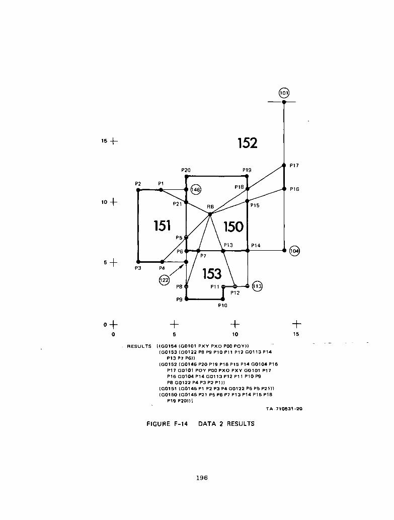
15
P2
10
P10
+5
+10
+15
RESULTS UG0154 (G0101 PXY PXO POO POYI)(G0153 (G0122 P8 P9 P10 P11 P12 G0113 P14
P13 P7 P6)l(G0152 (G0146 P20 P19 P18 P15 P14 G0104 P16
P17 G0101 POY POO PXO PXY G0101 P17P16 G0104 PI4 G0113 P12 P11 P10 P9P8 G0122 P4 P3 P2 P1I)
(G0151 (G0146 P1 P2 P3 P4 G0122 P6 P5 P21»(G0150 (G0146 P21 P5 P6 P7 P13 P14 P15 P18
P19 P20))l
TA-710831-20
FIGURE F-14 DATA 2 RESULTS
196

15 +
10 +
P10
P20
10
+
15
+
20
RESULTS (MAPCAR (FUNCTION RGNLIST) (RGNFND (GET VIEW <5POINTS$(IG0101 (POY POO PXO PXY)) (G0100 (POY PXY PXO POO))(G0099 (G0009 P1 8 P17 G0003)) (G0098 (G0016 P17 P16 P15I)(G0097 (G0062 P5 P4 P2 P1 P 20 P19 G0009 G0003 P17 G0016 G0043P10 P9 P8 P7)) (G0096 (G0074 P13 P14 P3 P2 P4 P5 P6» (G0095(G0074 P6P5 G0062 P7 PS P9 P11 P12)) (G0094 (G0074P12 P11 P9P10 G0043 G0016 P15 P16P17 P18 G0009 P19 P20 P1 P2 P3 P14 P130)
TA-710531-21
FIGURE F-15 DATA 3 RESULTS
197

P30 P29 P26P25
P34
P14 P16
RESULTS MDSKIN DATA4$
•(I SUPPOSEW DATA4$
EX2INEO
MODEL
(B (PXO POO) R (PXY PXO) T (POY PXY) L (POO POY) L23 (P33 P34)
L22 (P32 P33) L21 (P31 P32) L20 (P29 P30) L19 (P28 P29) L18 (P27
P28) L17 (P25 P26) L16 (P24 P25) L15 (P22 P23) L14 (P20 P21) L13
(P19 P20) L12 (P17 P18) L11 (P16 P17) L10 (P14 P15) L2 (P9 P14)
L1 (P34 P9»
CONJECT1
(8 (PXO POO) R (PXY PXO) T (POY PXY) L (POO POY) L23 (P33 P34)
L22 (P32 P33) L21 (P31 P32) L20 (P29 P30) L19 (P28 P29) L18 (P27 P28)
L17 (P25 P26) L16 (P24 P25) L15 (P22 P23) L14 (P20 P21) L13 (P19 P20)
L12 (P17 P18) L11 (P16 P17) L10 (P14 P15) L2 (P9 P14) LI (P34 P9)
GO001 (P31 P21) G0002 (P27 P23) GOOO3 (P24 P18) GOO04 (P19 P15)
CONJECT2
(B (PXO POO) R (PXY PXO) T (POY PXY) L (POO POY) L23 (P33 P34)
L22 (P32 P33) L21 (P31 P32) L20 (P29 P30) L19 (P28 P29) L18 (P27 P28)
L17 (P25 P26) L16 (P24 P25) L15 (P22 P23) L14 (P20 P21) L13 (P19 P20)
L12 (P17 P18) L11 (P16P17) L10 (P14 P15) L2 (P9 P14) L1 (P34 P9)
G0001 (P31 P21) GOO02 (P27 P23) GOOO4 (P19 P15) G0006 (P30 GOODS)
GOO07 (G0005 P33) GO020 (P26 P29) G0031 (P24 G0030) G0040 (P22
G0030) G0060 (G0058 P20) G0061 (G0058 G0030) G0059 (PI8 G0058)
G0071 (P16 P14))
EX2INED'
REGIONS
(IG0078 (POY POO PXO PXY)) (GO077 (POY PXY PXO POO)) (G0076
(P9 P14 P15 P19 P20 P21 P31 P32 P33 P34)) (G0075 (GO030 P24 P25
P26 P29 P28 P27 P23 P22I) (G0074 (G0058 G003O P22 P23 P27 P28 P29
P30 GOODS P33 P32 P31 P21 P2OI) (GOO73 (G0058 P20 P19 PI 5 P14 P16
P17 P18)) (GOO72 (G0058 P18 P17 P16 P14 P9 P34 P33 GOODS P30 P29
P26P25 P24 G0030)))TA-710531-22
FIGURE F-16 DATA 4 RESULTS
198
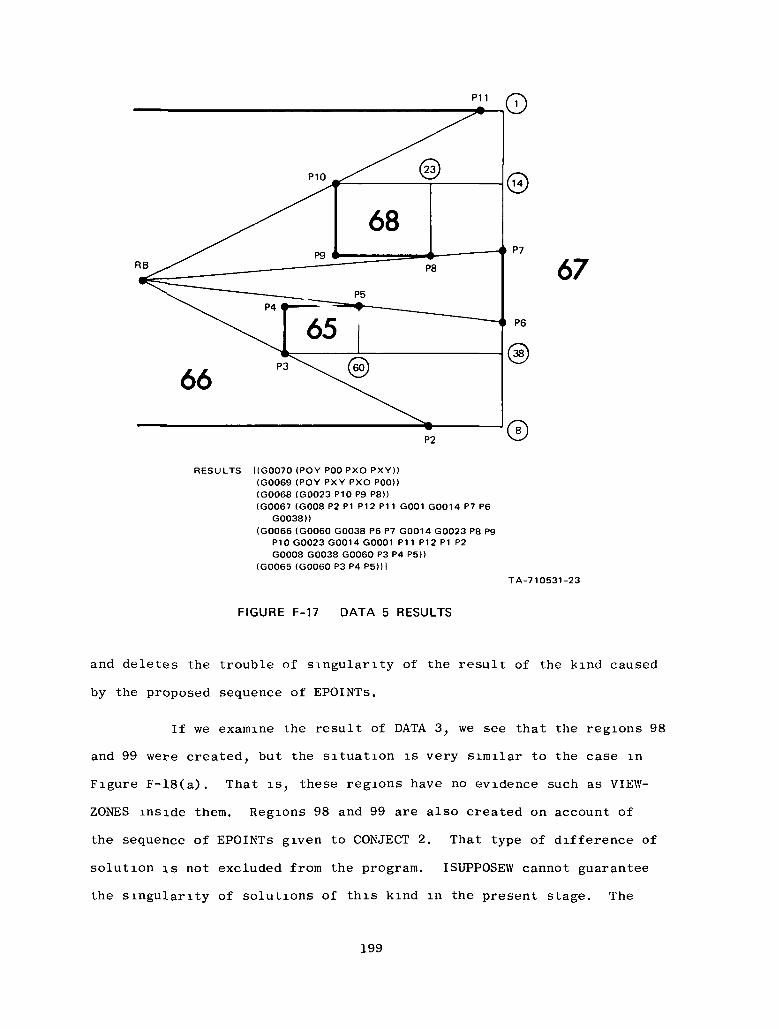
67
RESULTS [(G0070 (POY POO PXO PXY) )(G0069 (POY PXY PXO POO))(G0068 (G0023 P10 P9 P8))(G0067 (G008 P2 PI P12 P11 G001 G0014 P7 P6
G0038))(G0066 (G0060 G0038 P6 P7 G0014 G0023 P8 P9
P10 G0023 G0014 G0001 P11 P12 P1 P2G0008 G0038 G0060 P3 P4 P5))
(G0065 (G0060 P3 P4 P5))lTA-710531-23
FIGURE F-17 DATA 5 RESULTS
and deletes the trouble of singularity of the result of the kind caused
by the proposed sequence of EPOINTs.
If we examine the result of DATA 3, we see that the regions 98
and 99 were created, but the situation is very similar to the case in
Figure F-18(a). That is, these regions have no evidence such as VIEW-
ZONES inside them. Regions 98 and 99 are also created on account of
the sequence of EPOINTs given to CONJECT 2. That type of difference of
solution is not excluded from the program. ISUPPOSEW cannot guarantee
the singularity of solutions of this kind in the present stage. The
199

Tm\
\\
\4
R2
R4
1
\ /
Ti / R3
'
/I
\ /\ /VRB
/ R5
R6
R7 R8
RB
P2
L'
P3
TA-710531-24
(a) (b)
FIGURE F-18 EXPLANATORY DIAGRAM FOR CLOSING REGIONS
program that defines the relationship between regions must be added to.
Then inconvenient regions may be deleted from the results or may be
merged by the other (as they are most likely to be), but it must be
another problem concerned with the global conjecture.
B. The Problem of Overlap of Lines
The algorithm of CONJECT 2 has the problem of overlap of
created lines. ISUPPOSEW always replaces the, old line in the current
model by the newest line. It does conjecture procedures evenly on all
the EPOINTs listed in E*LIST at first, without deleting any that happen
to be considered to be connected as the result of the conjecture of
other points. The case (b) in Figure F-18 has three points, PI, P2,
and P3, to be dealt with by CONJECT 2. Assume the sequence given in
(.,. PI ... P2 ... P3 ...). When CONJECT 2 works on PI, the set of
lines such that the extended line of PI crosses I/ is created in the
model, CONJECT 2 is applied to P2, and the result becomes the same.
200

ISUPPOSEW replaces the old set in the model with the new result. This
is the way that ISUPPOSEW avoids the overlap problem, but it drives the
program to meaningless calculations.
C. Questionable Conjecture, Impossible Conjecture,
and Necessity of CONJECT 3
The basic concept of ISUPPOSEW includes the idea that an
EPOINT like P9 in DATA 1 seldom exists, which has no opposite EPOINT
to which it can be connected, in the building of the average kind. This
gives the basic reason to case (a) in Figure F-19 that the line must be
\\\\\
/ / \/ ,/ /
PM
L ^.
\j \
\
1 vPN
TA-710531-25
(b)
\\
(a)
FIGURE F-19 DIAGRAM FOR QUESTIONABLE CONJECTURE
extended in the direction shown by an arrow, for if that point is one
part of the doorway, it must be connected to the opposite one by CONJECT
1. The problem occurs when such opposites cannot be found because of
obstacles. Such a case occurs in rather complicated data, as is shown
in Figure F-19(b). Both points PK and PL must cross NVZNS to make
closed regions, because the opposite EPOINTs of them may be somewhere
behind LO. This is one point at which the author fears that CONJECT 3
is necessary.
201

We can consider more impossible conjectures. P3 in DATA 1 is
one of them. ISUPPOSEW has treated only EPOINTs. Consequently, although
they are in almost the same situation, conjecture on P5 in DATA 1 is
different from other points such as Pll and P10 in DATA 1.
Suppose the line LO in Figure F-19(b) is connected to the
other by CONJECT 1. There is left no possibility that the conjectured
line L is drawn. Then point PM has no chance to be connected to any
other point. Furthermore, who can guarantee that line L is right? The
best answer may be that the line L connects to LO on the central point
of LO. Now, it is impossible for ISUPPOSEW to make the above conjec-
tures, and the author thinks it is the limit of ISUPPOSEW and that of
human beings at the same time so long as we consider only the plan model
of a visual scene.
202

Appendix G
ROBOT COMMUNICATIONS BETWEEN THE PDP-15 AND THE PDP-10
by
B. Michael Wilber
203

Appendix G
ROBOT COMMUNICATIONS BETWEEN THE PDP-15 AND THE PDF-10
I INTRODUCTION
There are an inconceivable number of links in the chain from a
person typing English sentences on a Teletype to Shakey shaking, tweeting,
and occasionally moving from place to place. One of those links is a
package of subroutines through which the LISP part communicates with the
robot program in the PDP-15, via the POP-10 monitor, the infamous inter-
computer interface, and a set of PDP-10 communication routines on the
PDP-15. In this document, we will characterize the robot vehicle as it
is seen from LISP via this subroutine package; when we refer to the PDP-
15, it should be understood that we refer to the robot program within the
PDP-15.
This appendix is one of three documents describing the robot from
more or less the same point of view; the others are John Munson's
Technical Note 351 and a forthcoming description of the robot as seen
from the next level up.3 Technical Note 35 describes the overall design
considerations of this software and was written before any of the soft-
ware. Here we describe the implementation of the "lower end" (as pre-
viously detailed) of that software, as well as characterizing the
1"Bottom-Level PDP-10 Software for the SRI Robot," August 1970.
2Further details on the workings of the PDP-15 can be gleaned from
Ed Pollack's memos of 11 February 1971 and 18 March 1971 (two memos)
205

concomitant hardware as viewed through the software. Ihe third document
will complete the description by telling how to use the robot from the
viewpoint central to Technical Note 35. The last two documents, telling
how to use the robot, go into considerable detail superfluous to Technical
Note 35; areas of contradiction of Technical Note 35, however, represent
implementation-motivated changes in the design.
We will characterize the robot as having two levels of protocol.
The "PDP-15 protocol" is concerned with messages between LISP and the ,
robot (or at least the PDP-15), while the "PDP-10 protocol" treats the
ways of inducing the PDP-10 subroutine package to handle those messages.
The PDP-10 protocol is by far the simpler, so we shall consider it
first. A conversation with the robot program in the PDP-15 is initiated
or terminated by a call to INIT15 or REL15, respectively, about these
two nothing more need be said. During a conversation, messages are sent
to the PDP-15 by calls on START15; these messages typically start activi-
ties aboard the robot. Status reports are elicited from the PDP-15 by
calls on READ15. Finally, the subroutine package provides a fifth entry
point called STOP15, which sends a "stop" message; it is a specialized
entry to START15 and thus needs little further special consideration.
Before further exploring the peculiarities of START15 and READ15,
we will touch upon the PDP-15 protocol—the content of the messages
transmitted between PDP-10 LISP and the PDP-15 robot program. Munson's
Technical Note 35 introduces the concept of an "activity" as one of ten
motor or sensory actions that the PDP-15 can be asked or told about. In
communication with the PDP-15, these activities are designed by code
numbers called "activity codes." There are certain other kinds of mes-
sages sent between the two computers (e.g., '"stop" above) which artifi-
cially fit into the protocol by the use of dummy "activity" codes. We
206

will however, try to restrict our use of the word "activity" to Munson's
sense and use "action" to denote this more general sense.
In order to further isolate the PDP-10 protocol from the PDP-15
messages, we have stylized the PDP-15 messages into two formats--one
for the orders sent to the PDP-15 ,(via START15), and another for the
status reports elicited from the PDP-15 (via READ15). Each of these
routines, of course, needs an activity code to identify the action under
consideration. The (START15) orders also contain an additional optionally
used parameter giving—for example—a distance to turn. The (READ15)
status reports contain a value called the "activity status value" (ASV)
and two additional values (which may or may not be used). The ASV sum-
marizes the status of the action in a fairly uniform way, while the
additional values give additional information in a manner peculiar to
the particular action under consideration.
There are two additional facets of READ15 that will bear passing
mention. For completeness, we should mention that READ15 sends the
activity code to the PDP-15 in the request for a status report, so it
is not entirely passive with respect to the PDP-15 robot program. Far
more important is the observation that some of the actions do not
directly affect the vehicle, but are instead handled completely by the
PDP-15 robot program. For these actions there is no corresponding
status report; in fact, we do not consider the case of READ15 being
given one of the corresponding activity codes.
207

II THE PDF-10 PROTOCOL
A. The LISP Functions in the PDP-10 Protocol
We will now specify the precise LISP constructs used in the
PDP-10 protocol. The reader may be interested to note that this is a
LISP adaptation of the FORTRAN-orlented protocol.1
1. Establishing the Connection: (INIT15)
This must be done when the program is started or re-
started. Thus it must be done whenever the PDP-10 monitor detects an
error and stops the program. Spurious execution of this form should do
no harm.
2. Breaking the Connection: (RELL5)
This is the complement of (INIT15).
3. Sending an Order: (START15 actcode param)
Execution of this form will send an order to the PDP-15
robot program; the order will contain the values of "actcode" and "param.'
The PDP-15 will then usually start the action represented by "actcode,"
with "param" specifying, say, a distance to turn; details- are further
specified by the PDP-15 protocol.
4. Reading the Status of an Activity: (READ15 actcode)
This is a pseudo-function in that it returns values via
global variables as well as communicating with the PDP-15. It sends a
1Cf. Ann Robinson's memo of 26 June 1970.
208

request for a status report to the PDP-15 and then reads the resulting
report from the PDP-15, the request contains the value "actcode." The
activity status value is returned as the value of both the function and
the LISP atom ACTASV, while the first and second additional activity
status values are returned as the values of the LISP atoms ACTV1 and
ACTV2, respectively. (These three values replace the values current
when the READ15 function is entered at the same level of binding. Thus
the effect is the same as if the atoms had been SETQ-ed to the values in
the calling function.) Further details are given by the PDP-15 protocol.
5. Stopping an Activity: (STOP15 actcode)
A "stop" order is sent to the PDP-15, the order contains
the value "actcode." While this is not a separate activity1 in the
PDP-10 protocol, it is a separate action in the PDP-15 protocol, to
which the reader is referred for further details.
B. How to Use the LISP Functions in the PDP-10 Protocol
1. The Connection—INIT15 and REL15
Before a conversation between LISP and the PDP-15 robot
program can take place, a connection must be established by INIT15. This
connection is broken by REL15 and also by the monitor or the LISP system
on a large number of monitor commands, such as RUN, SAVE, START, etc.,
and must subsequently be reestablished.
Ideally, one will break the connection with REL15, but
the monitor's (and LISP's) predilection to do this automatically as a
by-product of many frequently used operations reduces REL15 to near-
vestigial status.
1 In the sense of Technical Note 35.
209

2. Using the PDP-15 Protocol—START15, READ15, STOP15
A conversation, as specified in the PDP-15 protocol, is
carried out by means of the START15, READ15, and STOP15 functions. As
previously mentioned, these functions can only be used after an INIT15,
any further restrictions on their use is the domain of the PDP-15
protocol.
Ill PDP-15 PROTOCOL
A. The PDP-15 Actions in the PDP-15 Protocol
There are twelve actions that the PDP-15 can be commanded to
perform, eight of these actions are just the PDP-15 ends of Technical
Note 35 activities, while the others serve other purposes. All twelve
actions are detailed below. Eight of these actions directly cause the
PDP-15 to send orders to the robot and receive responses from the robot,
while the others affect various aspects of the operations of the eight
robot actions. We will now briefly describe the PDP-15 actions, but we
defer details to our summary. Many of the actions executed by the robot
can terminate abnormally; we defer discussion of that point to a suc-
ceeding section.
1. Stop
The indicated activity is stopped. The activity must be
tilt, pan, iris, focus, roll, or turn. The activity status value for
the stopped activity is set to 7, and the rest of the report will cor-
rectly reflect its terminal status.
2. Tilt
The robot's head tilts by the indicated amount.
210

3. Pan
The robot's head pans (relative to its body) by the indi-
cated amount.
4. Turn
The entire robot turns by the indicated amount. Note that
roll and turn conflict in their use of the wheels.
5. Roll
The entire robot rolls forward or backward by the indi-
cated amount. Note that roll and turn conflict in their use of the
wheels.
6. Override
The catwhiskers and pushbar are overridden according to
a code word supplied by the most recent override order. This override
is effective on rolls and turns.
7. Range
This is a complex action, which we will describe in terms
of its components. Upon receipt of the START15-order, the rangefinder
is turned on and allowed to start warming up. When the rangefinder
finishes warming up, the PDF-15 reads the value from the rangefinder
into its own memory. At this time, the PDP-15 starts timing an interval
after which, barring another START15-order from the PDP-10, it will
automatically turn off the rangefinder. If another START15-order comes
from the PDP-10 during this interval, the PDP-15 reads the then-current
rangefinder value into its memory and resets the interval to turn off
211

the rangefinder. Thus a sufficiently rapid succession of rangefinder
STARTlS-orders will keep the rangefinder turned on. READ15 will always
report the value resulting from the START15 rather than directly reading
the rangefinder, so READ15's will normally be paired to STARTlS-orders.
8. Emergencyfinished
This "action" cannot be the subject of a STARTlS-order
but supplies a means by which the PDF-15 can supply (via READ15) infor-
mation to the PDP-10 regarding its "emergency" recovery status. Further
details are given below.
9. Tvpoweron
This is a complex action quite similar to range in that
it entails a warmup phase and a "kept-on" phase that is reinitialized
on subsequent STARTlS-orders. This action, however, does not directly
read a TV picture, owing to problems in handling the enormous volume of
data that would result therefrom.
10. Iris
The TV camera's iris setting is changed by the indicated
amount.
11. Focus
The TV camera's focus setting is changed by the indicated
amount.
212

12. Initialize
The PDP-15 resets itself to its initial state. Note that
this involves turning off the overrides. No orders are sent to the
robot because no on-board initialization is necessary. Note that any
on-board actions can thus be in progress. The PDP-15 will not become
confused about this. This action is used in system initialization and
also in certain error recoveries (see below).
B. How to Use the PDP-15 Protocol
1. Establishing and Terminating Rapport
When first establishing contact with the PDP-15, it is
advisable, though by no means necessary, to send it an initialize order.
Then the PDP-15 and the robot will be in a more-or-less well-known state.
No means is provided by which the contact can be broken because there is
no need for such an action.
2. Normal Operations
Any PDP-15 action except emergencyfinished can be the
subject of a START15-order whenever there is no conflict with an in-
progress action, this is not quite true in the case of emergency re-
coveries, as we will discuss below. Emergencyfinished can never be
START15-ed. The conflicts are as follows.
(1) Override and initialize are completely
executed in the PDP-15 and thus are
never in progress.
(2) Stop sends orders to the robot but
works by affecting other actions and
is thus never in progress itself.
213

(3) Each of the remaining eight START15-able
actions conflicts with itself while it
is in progress.
(4) Roll and turn conflict with each other
while they are in progress.
Any of the eight on-board actions—as well as emergency-
finished (i.e., any action but stop, override, or initialize)—can be
reported by READ15 at any time. The range of values that can be taken
by the activity status variable changes from action to action, but there
are five standard values with roughly the same meaning for each of the
actions. They are•
-1. The action is in progress. For range
and tvpoweron, this means that the on-
board equipment is warming up.
0: The action has completed normally.
6: The action did not complete in the time
the PDP-15 allowed it. The PDP-15 then
took other measures to terminate the
action.
7: This action was specified in a stop
order.
8- An "emergency" was noted by the robot,
the PDP-15, or by the telemetry inter-
face between them. Recovery from this
condition is further discussed below.
Other conditions can give rise to values from 1 to 5 as individually
noted in the summary below.
214

3. Coping with an 'Emergency
Under certain drastic conditions (e.g., transmission
error or low robot power) the PDP-15 may report an activity status of
8. Owing to the gravity of this condition, the PDP-15 will not com-
pletely reset itself until it has received acknowledgment that the PDP-10
has noticed. For example, the PDP-10 cannot presume correct execution
of recent orders or even nonexecution of nonorders. The PDP-15 will
attempt to reset the states of the robot, as well as some of its internal
tables, but will not complete the job until receipt of an initialize
order from the PDP-10.
In addition, we must consider timing. The PDP-15 takes
several seconds in its attempts to reset the state of the robot. It
tells the PDP-10 about the progress of this recovery by means of a
special activity code--and the associated activity status variable.
This special activity is the "emergencyfinished" action. Its activity
status variable is set to 8 (just as all the others) when the PDP-15
perceives an emergency, but it is automatically set to zero when the
PDP-15 and the robot have again established communications.
Thus there are two things the PDP-10 must do upon per-
ceiving a PDP-15 "emergency" (i.e., activity status variable = 8). It
must send an initialize order, and it must wait until the emergency-
finished activity status value goes to 0. These can be done in either
order, but both must be done. It should be noted that successful com-
pletion of this part of the protocol does not guarantee absence of the
offending condition, e.g., low power on board the robot.
C. Abnormal Terminations on Board the Robot
We have discussed PDP-15 conditions under which actions can
terminate abnormally (e.g., timeout, emergency). There remain, however,
215

conditions on board the robot that can also abnormally terminate actions—
for example, bumping into an unexpected obstacle. Whenever a stepping
motor is thus abnormally stopped, the residual count is accurately re-
ported in the corresponding status report. These conditions are dis-
cussed below.
1. Tilt, Pan, Iris, Focus
These four motions are restricted to definite ranges by
limit switches. Whenever the indicated count would cause motion past a
limit switch, then motion is stopped at the limit switch and the status
report reflects this state.
2. Roll and Turn
There are four principal ways in which a roll or turn
can terminate abnormally, these are denoted by distinct values of the
READ15 activity status variable. First, the robot can engage a cat-
whisker and stop because of that. Secondly, the pushbar can come free
(because an object the robot is pushing has slipped off), causing the
PDP-15 to stop the robot. Also, the robot can encounter an immobile
obstacle while pushing (or preparing to push). (This case will be
treated more fully below.) _These three circumstances all involve the
robot stopping; however, the status reports also distinguish a fourth
case in which the robot covers the entire distance ordered by the PDP-10,
in spite of the catwhiskers being engaged sometime during or before the
roll. This could happen because the catwhiskers are overridden or be-
cause the catwhiskers became free either before the robot had finished
decelerating to a stop or before the roll started.1
1 See Ed Pollack's memo of 18 March 1971, "Robot Emergencies," Note that
his "pushbar emergency" is just the "hard contact" referred to herein.
216

When the robot encounters an immobile obstacle it backs
away: if it was rolling, it backs up to free itself, if it was turning
(unlikely, but still a distinct possibility), it turns back to its
original heading. This is a reflex in the PDP-15 because of the way
the hard-contact pushbar switch is connected to the PDP-15. That is,
the PDP-15 can sense the event of making hard contact but not the state
of being in hard contact. Consistent with our philosophy of removing
all possible computational burden from the PDP-15, we adopted this solu-
tion, rather than have the PDP-15 ensure that a subsequent roll or turn
be in a direction appropriate to releasing the hard contact. At any
rate, the status report of a roll or turn correctly reflects the ter-
minal status of the activity.
IV SUMMARY
A. Introduction
A LISP program communicates with the robot through the PDP-10
monitor and various programs in the PDP-15. We break the protocol into
two pieces, which we call the PDP-10 protocol and the PDP-15 protocol.
We can think of the PDP-15 protocol as treating the messages to and
from the robot, while we can view the PDP-10 protocol as treating the
way a LISP program gets the PDP-10 monitor to handle these messages.
Thus in this discussion, the robot is viewed as part of the implementa-
tion of the PDP-15 protocol. In previous sections we have emphasized
the meanings of messages at the expense of their precise forms, now we
will focus on precise formats and allude to the meanings only in passing.
217

B. PDF-10 Protocol
1. The Connection
(a) Execution of the form
(•INIT15)
will establish a channel to the robot
program.
(b) Whenever the form
(REL15)
is executed, the channel is disestab-
lished. In practice there should be
little need to execute this form.
2. The Messages
(a) LISP can send an order by executing
(START15 actcode param) _,
where the order contains actcode and
param and is subject to the rules of
the PDF-15 protocol.
(b) Whenever a LISP function is curious
about the state of a PDF-15 action,
it need only execute
218

(READ15 actcode) ,
where actcode specifies the action
according to the PDP-15 protocol. The
activity status value is returned as
the value of the function and of the
atom ACTASV, while the first and second
additional values are returned as the
values of ACTV1 and ACTV2; respectively.
(c) A LISP function can stop some actions
by executing
(STOP15 actcode) ,
which in the PDP-15 protocol is equivalent
to
(START15 stopcode actcode) ,
with "stopcode" being the activity code
for the "stop" action of the PDP-15
protocol.
C. PDP-15 Protocol
1. Formats of Parameters, Results, and Other Diverse Quantities
We frequently include in PDP-15 messages various numeric
and coded values. We will briefly digress to explain the formats of the
code words for the catwhiskers and the overrides as well as the peculiar
formats for stepping motor counts and residual counts.
219

a. Catwhiskers
The states of the catwhiskers and pushbar (after a
roll or turn) are encoded into a word called the "whisker word." The
pushbar and each catwhisker is associated with a unique bit position in
the whisker word, and the value of any given bit is 1 when (and only
when) the associated catwhisker is in contact with something (presumably
a box, wall, another robot, etc.). All unused bits in the whisker word
contain zeroes, so the entire word is zero when the robot is in an empty
area. The following table gives the correspondence between whiskers and
bits, of course, the pushbar bit reflects the "ready to push" switch,
not the "immovable object" switch.
Bit No. Octal Code Meaning of "l"
21 040000 Pushbar is engaged
23 010000 Left front whisker is engaged
25 002000 Front horizontal whisker is engaged
26 001000 Right front whisker is engaged
28 000200 Right rear whisker is engaged
30 000040 Rear whisker is engaged
33 000004 Left rear whisker is engaged
_ 35 000001 -Front vertical whisker is engaged
b. Overrides
The inhibition of rolling or turning due to the
pushbar becoming free or a catwhisker being engaged is overridden as
shown by this table.
220

Code Word Pushbar Catwhisker
0 Enabled Enabled
1 Enabled Overridden
2 Overridden Enabled
3 Overridden Overridden
c. Stepping Motor Counts
In the robot, motor counts are expressed in sign-
magnitude notation of various formats tailored to the individual activi-
ties. Because we have removed all possible computational burdens from
the PDP-15, this variability of format is carried up to the interface
between START15 and READ15 on the one hand and the lower-level LISP
functions on the other. We can characterize one of these sign-magnitudes
by two field widths: the width of the entire number and the width of the
significant part of the magnitude. Thus a 12-bit wide number of 11 sig-
nificant bits has no bits ignored, while a 12-bit wide number of 7 signi-
ficant bits has 4 bits (to be ignored) between the sign bit and the most
significant magnitude bit.
d. Residual Counts
Those actions involving a stepping-motor count all
return a residual motor count at the end of the action. (We expect that
on a normal completion, the residual count will be zero.) The residual
counts are treated nonuniformly for the following reasons.
The robot has two distinct ways of handling residual
motor counts: in the cases of a tilt, pan, iris, or focus action running
into a limit switch and stopping because of the limit switch, the sign
bit is inverted; in all other cases, the sign bit is correct. Fortunately,
221

these four actions can never overshoot their targets, and thus the
residual's sign bit is dispensable. (Of course, these four actions
could be aborted by the stop action or a PDP-15 emergency so the sign
bit is not even necessarily reversed.) On the other hand, the vehicle
can build up considerable momentum while rolling (e.g., down a ramp) or
even turning, causing it to overshoot and then back up to the target.
Of course, there is nothing preventing, for example, the pushbar coming
free on the overshoot, and so the robot could be on either side of the
target when it finally stops rolling (or turning). Then it is very
important to preserve the sign bit associated with the residual count
of a roll or turn.
The way residual counts are returned (via READ15),
then, is this: For the roll and turn activities, the residual count is
the correct signed residual count, while the other activities return
the magnitude of the residual count.
2. Formats of the Messages
The formats of the messages themselves are presented in
abbreviated fashion in Table G-l.
222

Llo
4-1
Ud
cO
CO
O
cou
4->
L,0ao
OS
in3
d
cn
ma
OS
cnc /-.O G)H -P
•P tB
(0 H0 X04 0
•p aH ae drl v_^
H /-v
> CN-H >
S B
d oC rH
0 XIH d
H L."O d•a >
cn•a 3C -P
y -P0) W
CO
•P f \H rH
3 By <
rH Qd rH
C XJO 0)H H
•P LiH d•a >•a< cn
3-P -Pcn dLI -PH CO
b-
^
G)
X)d
y L,< d
tn o
H 0a: e< dH I-co a
a
- o> "0-J O
y
^
o
S0
0co
(Vo•oy
y
o
a.0
«
a.3 a
30)
L, abo CD0) L,
•O bO\ CDin -D
3 COo +uO ui
+ T
ocO2
C
§U
rH
3
H
cn<D
O
cn
E,_,
cn ,*
C cn3 -P0 Hy X)
Li CN0 rH
•P \O CD
="
OrH
in <HO G)0 -H
be in
o Siai o\ T3cn
d rH3 rHO -fym mo orH rH
+ 1
DC02
C
O
d3•ain<v
y
cn
£,_,
cn .
3 -PO HU XI
L. CMO rH
O 00
CN
Cda
cn
30O
otnCD
1
(01
,
+
•
0
aE3XI J
•O 7OLiOd
H
cnd30O
0
0
c*
t
c
<HCD
tnoo
o•aoa>
3
3s
J<:nH
c
33J
Hfl33Hnj
•ooa
i a= 03 LI3 "O
13 TJj ai ai a:> O
n tn
,-v
•p_£
00
\
^
:
M4JC3Oyooo-f
**
',
4
•
c
J
1JJuor-J
O
tnc30y
o0s,
^
c
•adS
0<H
G)
'P.
m
1-1
3
Ua-n•H
:
j
33J
H•u3DH
ny£
<i_ii
'H
H ODU T3> CU2 •*1 d•< x»;j -p3. Un. oD •-)
n o
^^i5
XI
00rH
^
p
HD
OC02
nQJ
O2
•a0
ooo
o•oL.
oo
in-P -PQ> CO 3
<H Oy
m CDCO CN
CO
Q)C02
inc3Oy
•ac
0)bocd
CS
XT:G)
•cd
Q.3 Q.
3
c -aE S
S O S
1
"oco2
CD
0bDca
OS
G)CO2
GJCO2
C02
_>OXt -PO O '-N
LI x> inO G)
0 L. 3•P rH
bo dbO C >d HH Li Ll^ o orH c x:P H O
oc
moo2
1
O TJC 0a x:bo cnLi Ho c
ps "•
ac0
oo2
Oco2
•ooLl
•acd
a3 a
3boc -aH G)E EL. <fH L,
S O S
I
"aco2
X
eoosoaH
•DOC
E
G)
•d
G)XI
0H
01c02
C30yrHd3•ocnoOS
x:yH
sin
E
rH
cn .4,
c "tn3 -Po -<y xi
L. CM0 rH
0 ^
Ol
cn
**
T3G)
H
ELiO
Q)•aG)XI
0H
QJdo2
C30yrHd3•oHcno
OS
x:o
scn
E,_,
tn s-*.
C -P3 P0 X)y
OJL> rH
O \
0 ^H
O
m3yo
G)CO2
C02
"oCO2
to
O
d
C
— — Li
223

Appendix H
FORTRAN DISPLAY PACKAGE
by
John Bender
225

Appendix H
FORTRAN DISPLAY PACKAGE
This appendix is a follow-up to the User Display Software Memo of
October 1970, with corrections and specifics for using the display from
FORTRAN.
The current implementation is a minidisplay package that gives the
user the basic routines needed to display a figure. No light pen
facility has been implemented. A satisfactory handle for indicating
the location of a light pen hit within a user's sublist has not been
worked out. The ability to save, retrieve, and manipulate a complete
frame is not possible, and may not be a desirable low-level FORTRAN
facility. See the attached pages for a rewritten edition of pages 4, 5,
and 6 of the October memo.
The format of a sublist has been simplified and is as follows-
X position
Y position
e
e
X position
Y position
e is either an incre-
mental vector, an X
position, or a Y
position
— plus end of list
The left half of all sublist words is ignored. All sublists must con-
tain at least one end of list.
The operating procedure for using the display is as follows:
(1) Reserve the PDP-15 for your use, using the signup sheet.
227

(2) Turn on the power to the Adage display.
(3) Put the newest version of the bootstrap program in the
PDF-15 papertape reader.
(4) Put 07600 in the address switches.
(5) Press the following PDP-15 console buttons in order
(located in upper left-hand corner):
STOP
RESET
READIN.
(6) Log in on the PDP-10 and get on your disk areas,
DISMON.BIN and DIS10.MAC, from user area [20,26].
(7) Type the underlined:
.R T015J
FILE TO GO TO 15*1
DISMON.BINj
TC
(8) Along with your FORTRAN program, load the file DIS10.MAC.
The display is now yours.
(9) When finished with the display, turn off its power and
hit the STOP switch on the PDP-15.
228

To: AI Group , October 1970
From: Systems Programming
Subject: User Display Software
The following memo is divided into three parts:
Part I is a description of the way the display works at the lowest
level. It is provided for information only; it is not expected that
LISP or FORTRAN programmers will use this information directly.
Part II is a description of the display commands that are accessible
from FORTRAN or MACRO.
Part III is a discussion of a display user system (the user being
a LISP robot programmer) that we envision as the final working system.
We urge everyone to read this and offer criticisms. We do not wish
to omit any obvious functions and would like to accommodate all users if
possible.
LJC/kls
229

In the PDP-10 a display list is defined as a list of two-word
packets that describe sublists, where a sublist is a list of PDP-10
words that are the coordinates of a point on the user's screen. The
user's screen is a two-dimensional 10" X 10" area. For the purposes of
this description, any point outside this area is not visible. The X
and Y coordinates have the origin at the center of the screen.
The structure of a display list is as follows:
first
packet
location
lengthcontrol
word
X
position
e
e or e '
Y
position
e'
e or e'
(see below for
description of e)
Xposition
Yposition
\end of list must be setThe move bit is set if the vector is to be displayed at the inten-
sity specified in the Y portion of the position word.
The preceding description of a display list did not include any
mention of the various modes available to the user. The available modes
are: point, dashed, and line. The line mode is normally used to describe
a figure in a frame.
The control word contains the bits that indicate in which mode a
sublist is to be displayed. The entire sublist must be displayed in the
same mode. There exist two submodes for line: absolute vector and in-
cremental vector.
230

The control word bit definition is as follows:
<°*
e is an element that is either a description of an incremental
vector or the X portion of an absolute vector. e is either an incre-
mental vector or the Y portion of an absolute vector. Note that a sub-
list must start with an absolute vector. This requirement ensures that
the position of the display beam is well defined before the display
enters the incremental mode. Also, the sublist must end with the dis-
play in absolute vector mode, because only in the absolute mode is it
possible to have the end of list bit. End of list bit set defines the
end of a sublist.
An absolute vector has the following form:
e = X
j change to incremental if set
intensify bit
end of list bit must be off
e' = Y [intensity |
effectively 4 bits or 16 levels
In incremental mode,
e and e' = X increment | Y increment [ j |
t change to absolute if setintensify bit
231

The only functions available to user programs are: light pen enable,
line mode, point mode, and dashed mode. The user cannot disable, on, end
of list enable, absolute vector automatic, or display clock. The user
cannot enable, stop" enable, or manual. Scope enable may be indirectly
effected by the blink function. If the display is to be capable of
blinking a sublist, this function will have to be performed in the PDP-15.
232

PART II, Revised 2/1/71
User Display Software Memo, 10/70
The MACRO subroutine calls that are available to the user are-
CREFRM(framename)
ADDSL(name,length,mode)
DELSL(name)
Create frame, where frame name is a
block of storage in which the display
list packets will be stored, or are
stored if first entry is nonzero.
Add sublist; name is the address of
a sublist, length is the absolute
number of contiguous PDF-10 wordsused in the sublist, and mode is one
of the following:
1 line
2 dashed line
3 point
4 blink line
5 blink dashed line
6 blink point
Delete sublist, deletes the entry
and moves up the bottom of the list.
REPSL(oldname,newname,length,mode) Replace sublist.
MODE(name,mode)
LPON(name)LPOFF(name)
SET INT(name,value)
DISPLA
New mode, changes the mode of an
existing sublist.
Light pen on/off, enables or dis-
ables the light pen for this sublist.
Set intensity; changes intensity in
an existing sublist. The values can
be from 0 to 15
Display; will display the list at a
refresh rate of 40 frames a second,
using all entries in the array re-
ferred to by CREFRM.
233

HIT Hit , queries the PDP-15 if a lightpen hit has occurred since the last
time it was interrogated and returns
a sublist reference and an index
into the sublist; 0 otherwise. This
is not presently implemented.
STOP Stop, turns off the scope. This
does not have to be done before
changing what is currently appearing
on the display.
A copy of the current display is kept by the user. The only infor-
mation that he can get back from the display is light pen hit information.
Some routines that can help a user in building up a sublist are:
INCVEC(1ocation,Xincrement,Yincrement,action)
Incremental vector puts the X and Y increment
values in the specified location. Action has
values of:
0 Don't change vector mode, don't intensify
1 Change vector mode, don't intensify
2 Don't change vector mode, intensify
3 Change vector mode, intensify.
Changing vector mode only affects vectors that
follow the vector in which it occurs.
ABSVEC(location,Xposition,Yposition,action)
Absolute vector puts X position and action
value.in left half of location, and puts Y
position and implied intensity in right half.
The action values are the same as for incre-
mental plus end of list action:
234

4 End of list
5 End of list and intensify.
INTENS(value)
Implied intensity in constructing a sublist
intensity is an implied parameter and is
needed by ABSVEC.
GETINT
Get implied intensity returns the value of
the assumed intensity if no intensity value
is ever defined and an assumed value of 1010
is used. This is a FORTRAN function.
235

PART III
A. Introduction
This proposed display system is plagiarized from the BBN 940 LISP
system. That system, however, seemed to be designed around the BBN's
displays. Ours, we hope, is somewhat display-independent. Since our
display is quite primitive, this doesn't hurt.
The system centers around an internal LISP representation for struc-
tured pictures. Simple objects such as lines, quadratic curves, and
character strings are combined, translated, rotated, scaled, etc. by
combining them into lists together with key words and necessary
parameters. Currently, the system is designed to handle only two-
dimensional coordinates, but we hope everything will be easily extended
to homogeneous coordinates. Our system is unsuited for displays of
large numbers of unstructured points, say, a display of unprocessed TV
pictures. But for interactive systems displaying line drawings, such
as plots or pictures of rooms, the system offers flexibility of data
structure with a minimum of space and computation.
B. Noninteractive Picture Display
To display a picture the user must first construct the internal
representation. The proposed primitive figures are:
(1) (DVECTOR X Y X Y ) represents a vector from (X ,Y )
to (X Y
(2) (DPLOT A) (where A is a list of Y values, say
A = (Y ,Y ,...,Y )) represents a plot of the elementsl ^ n
of A at unit intervals along the X-axis
236

(3) (DPLOT AT) similarly represents a plot where A is
interpreted as X values
(4) (DCIRCLE X Y RDT) represents a circle with origin
(X,Y) of radius R; approximated by cords spanning
an angle of DT
(5) (DTREE E) represents a tree-like display of the
s-expr E
(6) Character strings; that will be discussed later.
To define a unit interval the display is thought of as a coordinate
system with the origin in the middle and extending one unit on each axis.
All numbers may, in normal list fashion, be fixed or floating.
A figure is either a primitive figure or modified figure. The
following list of modifications always apply to both kinds:
1. (TRANSLATE: F X Y) represents F translated by X Y
2a. (SCALE: F S) represents F scaled by S in both axes
2b. (SCALE: F X Y) represents F scaled by X in the X-axis
and Y in the Y-axis
2c. (ISCALE: F S) represents F scaled by 1/S in both axes
2d. (ISCALE: F X Y) represents F scaled by 1/X in the
X-axis and 1/Y in the Y-axis
3a. (MOVE: F A A A A ) represents the transforma-11 1 ^ 1 &£
tion of F by the obvious matrix
3b. (MOVE: F R) represents F rotated by R radians
4. (INTENSITY: F I) represents F displayed in intensity I
237

5. (DASH: F), (SOLID: F) (BLINKING: F) represents F
displayed point in the appropriate mode
6.' Finally, the list (F F ... F ) represents the com-1 2 n \
bination of the figures in the list.
Before we discuss the process of displaying an internal representa-
tion, let's consider an example. Suppose we have a list A = (Y Y ... Y )1 2 n
of values we want to plot. We would like everything to fit on display
and fill the screen. We also want to start plotting along the X-axis
at the origin. If DY is the maximum difference in Y values, then
(TRANSLATE:
(ISCALE:
(DPLOT A)
N
DY)
1 0)
is a possible representation. The LISP code to generate the figure
might simply be
(SETQ F (LIST (QUOTE TRANSLATE:)
(LIST (QUOTE ISCALE:)
(LIST (QUOTE DPLOT) A) .
(LENGTH A)(MAXDIF A))
0 1))
To convert an internal representation to a bit-string in the style
of the display the user might execute
(SETQ G (DISPLAY F A))
238

where F is a figure, A is the array in which the bits will go, and G is
a variable that will be used to store all sorts of good information about
A for later reference. G is thought of as a piece of glass and may be
shown at any time. The command (SHOW G) does just that. (KILL G) re-
moves G from the display. It is recommended that these pieces of glass
not be used as small picture parts but rather as major overlays. For
example, they might be a coordinate grid, a light button panel, an un-
smoothed picture, a smoothed picture, etc. It is planned that there
will also be a mechanism for modifying a piece of glass, but the specifi-
cations of such modification requests will be closely linked to final
implementation procedures.
The primitive figures for character strings are close to the LISP
print functions:
DPRIN1, DPRINC, and DTERPRI
They will be interpreted as the appropriate strings with character height
and width being some standard proportion of the display screen size.
DTERPRI will cause teletype-like lines to appear. The extra function
(DSPACES N) inserts N blanks. All the standard figure modifiers will
also work on character strings, permitting vertical printing and various
sizes.
C. Interactive Features
Since we are not yet sure just which selection devices will ulti-
mately be used, this proposal discusses everything in terms of the light
pen. Two facilities are offered for interactive graphics: the ability
to specify which figures may be selected and functions which will wait in
the PDP-10 until certain selections have been made through the PDP-15.
239

When a figure F modified by the list (ITEM: F), is processed by
DISPLAY special information is included in the bit buffer for the PDP-15
and notes are kept on the piece of glass in the PDP-10. Later, if the
figure is shown and the function (PENSELECT) is executed, the value will
be a pointer to the ITEM list in the internal representation of the
figure selected by the user.
This system is a compromise, and due to the cost of interaction be-
tween the machines it appears especially suited for light button panels,
selection of one from a few relatively disjoint figures, for drawing
with only a few lines. But since this is the anticipated kind of usage
the system should be adequate.
For drawing, two more interactive functions are needed:
(1) TRACE--which tracks the pen and returns as a value a
coordinate
(2) RUBBERBAND—which tracks to the first select, and
rubberbands until the second. It's value is the list
of the two selected coordinates.
240


![Artificial Intelligence · Artificial Intelligence 2016-2017 Introduction [5] Artificial Brain: can machines think? Artificial Intelligence 2016-2017 Introduction [6] ... Deep Blue](https://img.dokumen.tips/doc/110x75/5f0538917e708231d411e192/artificial-intelligence-artificial-intelligence-2016-2017-introduction-5-artificial.jpg)