Embed Size (px)
Citation preview

IPERMANENT RETENTION
REQUIREDBY CONTRACT II
::. :: --..,. !. ..-...., -.; . . .
,. ..,,., .,, .. . . .m. ..r. -.. .-r.- .Y, . . . ~,.,, -,... ’i...-, . .,, ..,.,, ,. ,-Al ““ i
.1-4 .,, .,,..> .+, . ...!i
., “, . ,., .,4 . ,., , . . . . . . . . . . . . . . . . . . . .! .,..
~ al:

. . . ,., .,;’,,.,.
&a Affiirive Actiora/Eqtasl Oppmtmity Ernpbya
‘.. .
. . ..F- . . . . .
. . . .,, . , . . . . .-.
.
.,
Thisthesiswasacceptedby TheUniversityofTexasatAustin,Austin,Texas,DepartmentofPhysicsinpartialfulfillmentoftherequirementsforthedegreeofDoctorofphilosophy.Itisthehdependentworkoftheauthorandhasnotbeeneditedby theTechni&lInformationStiff.
ThisworkwassupportedbytheRobertA.WelchFoundation.. . . . .,
“..
,
,./“ .’,! ..,. .
. .
i
,.”$
.,
-.
...- ... .
. . .
,, .. .,;, l.,,.. . .“. ,., ” ... ,,. . ,,, -
., .-., . :,
,.
,.,-. .
,’ ,’
-: .,. ... .
,.
.,, .ThIareprt was_xepqed as ~“;c~~t ‘o~wrk @b%d%$~J&en;y of the U&ted Stma Government.Neither the .L)sited Statq Covemrrsen~nor,any igeri~y thti~f,”nor any of their employees, makes my
WIITMty, ex@aa OF fipiied, or assumesany legal Iiabilit y or rcspnnaibifity for the accuracy, mmplet eneaa,.& uscTii of any information, apparatraa,product, or procear disclosed, or represents that its uscwouldnot MMge privately owned rights. References herein to any spe~k commercial product, proceaa,or=Ace by tra& name, !radeu<k, ~ufacturcr, or otherwise, does not neusaarily constitute or imply its
cndo~ment ;r&commen&tion, or favo~%y t~e ~Nte~ S&ka ~vcrraktent or ~ny agency thereof. The*Ad obiioN of au!hors expreaaed herein do nor neceasarify swe or reflect :hoae of the United
LA-8937-TThesis
UC-34CIssued: August 1981
-1
Inclusive Proton Spectra and
Total Reaction Cross Sections for
Proton-Nucleus Scattering at 800 MeV
John Alexander McGill
LOSNla~OS Los.lamos,NewMexico87545Los Alamos National Laboratory

TABLE OF CONTENTS
page
ABSTRACT . . . . . . . . . . . . . . . . . . . . . . . . . . . ● 0.V
CHAPTER I:
CHAFTER II:
CHAPTER Iv:
APPENDIX A:
APPENDIX B:
APPENDIX C:
Introduction . . . . . . . . . . . . . . . . . . . ...1
Experimental. Arrsmgement. . . . . . . . . . . . . . . . 7
Summary and Conclusions.. . . . . . . . . . . . ...32
Synopsis of the Data for Experiment 470 . . . . . . . .77
A Fast, Low-Mass Detector for Charged Particles . . . .84
Test Descriptor File... . . . . . . . . . . . . . ..95
ACKNOWLEDGMENT. . . . . . . . . . . . . . . . . . . . . . . . . . .97
REFERENCES. . . . . . . . . . . ● . . . . . . . . . . . . . . . . .98
h
.

1
.
INCLUSIVE PROTON SPECTRA AND
TOTAL REACTION CROSS SECTIONS FOR
PROTON-NUCLEUS SCATTERING AT 800 MeV
by
John Alexander McGill
ABSTRACT
Current applications of multiple
the elastic scattering of medium energy
scattering theory to describe
protons from nuclei have been
shown to be quite successful in reproducing the experimental cross
sections. These calculations use the impulse approximation, wherein
the scattering from individual nucleons in the nucleus is described by
the scatering amplitude for a free nucleon. Such an approximation
restricts the inelastic channels to those initiated by nucleon-nucleon
scattering.
As a first step in determining the nature of p + nucleus
scattering at 800 MeV, both total reaction cross sections and (P9P’)
inclusive cross sections were measured and compared to the free p + p
cross sections. We conclude that as mch as 85
nucleus proceed from interactions with a single
and that the impulse approximation is a good
% of all reactions in a
nucleon in the nucleus,
starting point for a
microscopic description of p + nucleus interactions at 800 MeV.
v

CHAPTER I
INTRODUCTION
The internucleon spacing in
the dellroglie wavelength of an
information suggests that 800MeV p
nuclear matter is about 1.3 fm, and
800 MeV proton is 1.5 fm. This
+ nucleus elastic scattering data
should be sensitive to the onebody density of the target nucleus;
several multiple scattering theorie~’-’) attempt to describe
quantitatively the scattering process in terms of the fundamental
protomnucleon interactions.
Current multiple scattering theory is an outgrowth of earlier
attempts to explain the scattering of elementary particles from complex
nuclei. Due to the partial transparency of the nucleus to low energy
(5)neutrons, a theory was developed which considered the projectile as
incident on a sphere of material characterized by an absorption
coefficient and an index of refraction. Such an “optical” model
provides good agreement with data for projectiles whose wavelength is
significantly longer than the internucleon distances.
For projectiles having wavelengths shorter than internucleon
spacings, the earliest attempt to obtain a microscopic theory of
(6,7)scattering resulted in the Impulse Approximation of Chew . ‘he
assumptions under which the model is valid are that the scattering
takes place on a single nucleon, and that the distortion and binding
.effects of the nuclear mediua are negligible. Binding corrections and
ec,m(deg)
I&’2MPb (p. P)
105 -800 MeV
10’ -ELASTIC
~3 -
lot -
< Iol -
~ Do -
Gy 10-1-
b= 0-2-
ld -
to-’-
W - “....,-
l+~’ ;’,;’ ! 1 I 1 I I ! ! I 1 I I ! I16 20 24 28 32 36 40 44
f)c,m(deg)
104 I , 8 # I I I
PROTONELASTICSCATTERING“e 800 MeV
,02
<1o’
20~lo
Yb 10-’u
,0-2
I0-3
1 ! 1 , I 1
10 12 14 16 18 20 22 24
ec,m(deg)
P
.
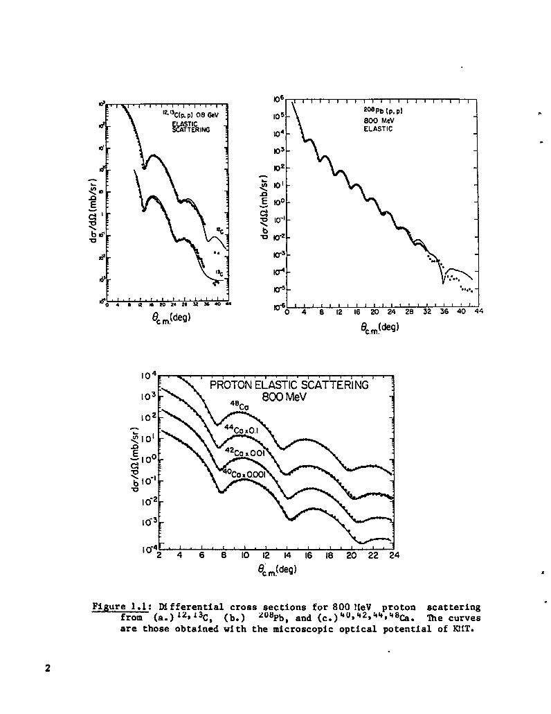
Figure 1.1: Differential cross sections for 800 MeV proton scatteringfrom (a.) L2S~3C, (b.) 2“8Pb, and (c.)qiJ,It2,W,148~C The curvesare those obtained with the microscopic optical potential of KllT.
2

multiple scattering terms were later introduced as refinements to the
theory.
Watso~l-3) married the optical model with the impulse
approximation, showing rigorously how to construct an optical potential
from the single scattering amplitudes. Such a construction provided
the theoretical justification for the use of an optical potential
calculated from nucleon-nucleon scattering amplitudes and the ground
state density distribution. Kerman, ~kllanus, and Thale~8)
reformulated the Watson expansion in a form more readily suited to the
use of “free” nucleon-nucleon amplitudes. Figure 1.1 shows the success
of the KMT theory in describing 800 MeV p + nucleus elastic scattering
(13,23,25)from various nuclei .
lbth the KMT and Watson Multiple Scattering theories solve the
SchrGdinger equation in integral form
Y+= 0+ GV4Y+ ,
where A projects out antisynmetrized states and
-1G=(E_Ho_HA+ic) ,
by defining a scattering matrix T such that
TO= VY+ .
(1.1)
(1.2)
With this definition Equation 1.1 becomes
3

T= V+ VG$T .
The KMT approach involves defining a single scattering operator
.(1.4);i = vi + ViGhti
where ~i is the amplitude for scattering from the ith nucleon, when vi
is defined such that
Azvi=Av=V . (1.5)
i=1
Using the definitions in Equations 1.4 and 1.5 in 1.3, and iterating
1.3, gives
T= A; + (A-l)iGAT . (1.6)
To cast the problem in a proper LippmanrrSchwinger form, the auxiliary
operator T’ is defined
A-1T’=7T
1
so that Equation (1.6) becomes
T’ = (A-l); + (A-l)k&’ .
(1.7)
(1.8)

.
.
From Equation (1.3) it is desired to provide an optical potential U
such that
T= U + UGPT (1.9)
where the operator P projects out the elastic states only, and its
complementary operator Q projects out only inelastic states. Of course
P+Q=~ . (1.10)
lJith T’ as given in Equation (1.8) the corresponding requirement for
the optical potential is
T’ = U’ + U’PGT’ . (1.11)
Solving Equation (1.8) for T’ and substituting into (1.11) gives
u’ = (A-1);+ (A-l)u’GQ; . (1.12)
The treatment up to this point is exact, and if the microscopic
single scattering amplitudes defined in Equation 1.4 were known, the
optical potential could be constructed. Unfortunately these amplitudes
which describe the proto~nucleon interaction in nuclear matter are not
known, and practical calculations approximate these amplitudes with
free nucleownucleon amplitudes , and the series in (1.12) is truncated
at some point. The use of free p+ p and p + n amplitudes in place of
A
t constitutes the impulse approximation in the context of multiple
scattering theory.
(he important consequence of the use of the impulse
approximation is that, within the context of the theory, all reactions
(9-11)must evolve from quasi-free doorways . In other words only
quasi-elastic and quasi-free plon production mechanisms are allowed to
initiate the process leading to reactions. Clearly unless these two
processes account for a substantial portion of the physical reaction
cross section, the theory will be inadequate.
As a first step in determining the nature of the 800 MeV
p + nucleus reaction mechanism, both total reaction cross sections and
(P,P’) inclusive spectra at forward angles were measured-
Chapter II describes the experiments, while Chapter 111
contains a description of the data analysis. Finally Chapter IV
contains a comparison of the total reaction cross sections with the
angl-integrated inclusive (p,p’) cross sections, and with predictions
(35)given by KMT calculations .
We tentatively conclude that two-nucleon processes account for
about 80% of the 800 MeV p + nucleus total reaction cross section, and
that the impulse approximation appears to be a good starting point for
microscopic calculations of p * nucleus observable at 800 MeV.
-,
.
.

CHAPTER II
EXPERIMENTAL ARRANGEllENT
Both experiments were done using the High Resolution
Spectrometer at the Los Alamos Meson Physics Facility. A brief
description of the beam line and spectrometer system is given in
Section A; Experiment 470 “Reactive Content of the Optical Potential”
is fully described in Section B; and Section C describes Experiment 386
“Total Reaction Cross Sections for p + Nuclei”.
A. BEAM LINE A1$DSPECTROIIETER— —(12)
The LAIPF LINAC has been extensively described elsewhere .
Briefly, both H+ and H- ions are accelerated to 750 keV by separate
Cockroft-Walton injectors at which point they are passed to the second
stage or Alvarez section (drift tube), where they are accelerated to
100 lleV. The third stage, the sidecoupled cavity section, then
accelerates the ions to 800 lleV.
Once the final velocity of 0.84c has been reached, the H+ and
H- beams are separated by a dipole magnet and each proceeds to
different experimental areas. Line A takes the H+ to several meson
production targets, thence to a beam dump. Line X accepts the H- beam
wherein it is focussed and steered onto a stripper. At the stripper a
fraction of the H- ions are relieved of their electrons then bent via a
dipole into Line C (see Figure 2.1). The unstrapped H- continues to
other experimental areas.
7

III
;
I
$..,...bI
,3s
23 9s
~. ..””
CJ
u-lo
.

4
-’
Blanpied has given a good description of the Line C be~
(13)optics . The beam line basically consists of three sections:
dispersion, twister, and matching. ‘he beam is dispersed in the
horizontal plane by a pair of dipole magnets. Beam phase space is then
rotated 90° by a set of five quadruples. Additional quadruples are
then used to provide a beam on target whose dispersion is matched to
that of the HRS for operation in the energy-loss mode.
‘IheHRS is a QuadrupoleDipoleDipole (QDD) system mounted in a
(14)vertical plane . ‘he optics provide parallel-to-point focussing in
the nomdispersion direction (~) and point-to-point focussing in the
A
dispersion (x) direction. Proper dispersion matching between the line
C optics and the HRS optics ensures that (apart from the kinematical
~) all scattered particles having the same energy loss at the target
will be focussed atA
the same transverse coordinate (x) on the focal
.plane. For a narrow beam in the y direction, the focal plane
coordinate in the non-dispersion (~) direction is proportional to the
scattering angle.
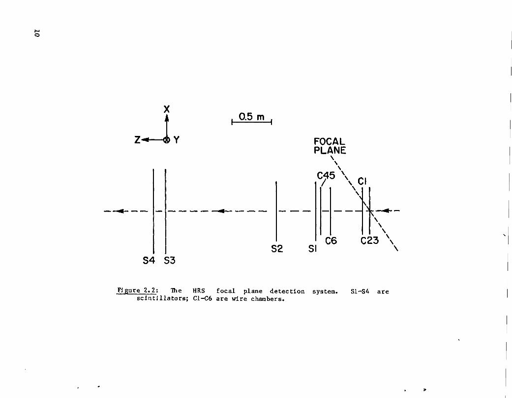
A schematic of the HRS focal plane detection system is shown in
Figure 2.2. Cbunters Cl through C6 are delay-line (DL) and drift
chambers (DC’s) which provide position and angle information; S1-S4 are
scintillators which give pulse height and tine-of-flight information,
1
and provide the “event” trigger. me
a wide variety of purposes and only
experiments.
detection system is designed for
portions of it were used in these
9
/
I Emo“
i.“”
III
U)
Ntn
I*
Iu
)
It
“
EJ
u;G.sul-in.fu
$4
I
I
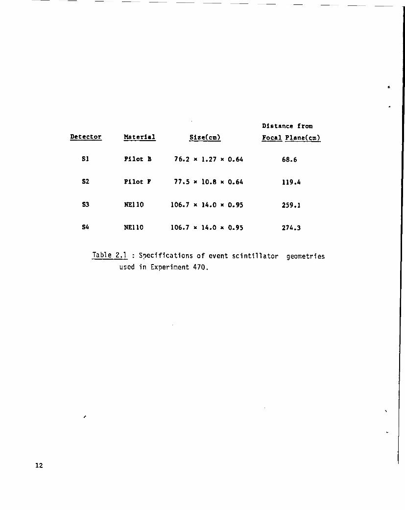
The four scintillators are optically coupled to EM1 9813B
photomultiplier tubes at each end. The physical characteristics of the
scintillators are listed in Table 2.1. ‘he anode signal from each
photomultiplier is
each scintillator,
fed into an LRS
input to an LRS 621 leading edge discriminator. For
the two discriminator signals (top and bottom) are
624 Ileantimer, tk output of which is a signal whose
arrival time is independent of position in the scintillator. Normally
the meantimed signals are used to form a four-fold coincidence, so that
a good event is defined by the requirement of S1.S2.S3.S4. This
constitutes the HRS event trigger, alerting other electronics modules
in the system that a good event (i.e. not a random charged particle
from room background) has occured and other data, e.g. chamber
information, may be read in.
Another function of the focal plane scintillators is the
identification of particle types at the focal plane. For a given field
setting the HRS will transport to the focal plane different particle
types with the same value of p/q, where p is the particle momentun and
q is its charge. Field settings corresponding to an 800 lleV proton
(p/q = 146311eV/c*e) also transmit a 500MeV deuteron, a 35011eV
triton, a 70 NeV %e, and a 1330 NeV n+. Therefore some scheme of
particle identification (PID) at the focal plane is necessary. ‘!iheHRS
system provides PID through measuring time of flight between two
scintillators, and pulse height in one scintillator. Time of flight
1 Egoes like ~or—. Pulse height from a scintillator is a function of
P
Distance from
Detector Raterial Size(cm) Focal Plane(cm)
S1 Pilot B 76.2 x 1.27 x 0.64 68.6
S2 Pilot F 77s5 x 10.8 X 0.64 119.4
S3 NEllo 106.7 X ]4.0 x 0.95 259.1
S4 NE110 106.7 X 14.0 x 0.95 274.3
Table 2.1 : Sy?cifications of event scintillator geometries
used in Experiment 470.
\
.
12
—

the energy lost in the scintillator , which is proportional to [~j2.P
‘Ihusparticles having different masses or charges can be distinguished.
In Figure 2.2 Cl and C6 are “delay line” (DL) chambers which
provide information redundant to C2-C5, “drift” chambers. (bnsequently
Cl and C6 were not used in this experiment. Each of the four drift
chambersA
used contains a pair of planes for x information, and a pair
for ~ information. The design and construction of these detectors has
(15,16)been dfscussed extensively in the literature 9 and only a
qualitative description is given here.
A schematic representation of a plane is shown in Figure 2.3.
Alternating anode and cathode wires are spaced 4 mm apart, with anode
wires attached at regular intervals to a delay line, and cathode wires
bussed together and grounded..
Each physical unit (stacked x-plane,
~-plane, ~-plane, ‘~plane) is covered with .001” aluminized Nylar. A
mixture of Argon, C02t methylal, and isobutane in the chamber serves as
an ionizing mediun; i.e., a charged particle traversing a plane will
produce ion-electron pairs which are accelerated to their respective
wires. Electrons in the vicinity of the anode will cascade, providing
a signal on the order of a few millivolts which passes in both
directions down the delay line. The arrival times of these signals are
‘1 = td+ n At ,
where td is the drift time in the gas, n is the nunber of wire
13

>
.-LI-1I
I
A
I
11
e+1 I
n-J

.
.
.
intervals between the left edge and the event wire, and At is the delay
interval of each wire space; and
t2= td+ (t-xl) At ,
where k is the total nunber of wire intervals between the left and
right edges. The time difference
tl- t2= 2nAt- gAt
reveals the event wire , while the time sun
tJ+t2= Ztd + iAt
yields the drift time td. In both quantities the constant %At can be
treated as an offset and renoved either in hardware with appropriate
delays, or in software. Thus the time difference locates the event to
* 4 mm, and the time sun is used to interpolate from there.
Figure 2.4a is a spectrum of time difference showing discrete wire
positions; Figure 2.4b shows a drift spectrum of t,+ t2. These data
were taken by illuminating the focal plane uniformly. Note that a
constant drift velocity would result in a flat drift spectrum out to
4mm , and zero from there out. Nonlinearities as in Figure 2.4b are
accommodated by generating a look-up table which gives the drift time to
position conversion in increments of -0.1 mm.
15

oL+-} i
u’)1-Z300
TIME DIFFERENCE
,~
-i
TIME SUMS
Hgure 2.4: Histograms of the difference and sun of the arrival timesof the signals from the left edge of an anode plane (tl) and theright edge (t2).
●
✎
16

*
.
lhere is one ambiguity
did the event occur to the left
the reason for placing two
remaining in the location of the event:
or the right of the anode? Here enters
Fy pairs in each physical unit. By
locating the event to within this ambiguity in two planes which are
offset by 4 mm, four possible combinations can be formed: (left,left),
(left,right), (right,left), and (right,right). One of these
combinations
and that one
tice
will ninimize the difference between the two positions,
is chosen.
accurate positions in all chambers are known, it is a
simple geometric problem to generate the variables of interest at the
focal plane : (xf, yf, Of, ~f), where Of is the angle in the dispersion
plane and @f is the angle in the non-dispersion plane. These four
quantities along with the inverse transport matrix and dipole field
settings are sufficient to determine the properties of the scattering
event. In particular the quantity
Pod= - Psp
l’sp
yields the momentun of the event (Po) relative to the spectrometer
central momentun (P5P), known from the field settings. The
relationships between the quantities are given by

,.
Y~
et
‘$t
6,,
5
0.00 0.00 -0.0644 0.1906
007471 -0.8125 0.0818 0.0007
-0.0229 0.0409 -5.0249 -0.1654
I0.0555 0.0002 0.00 0.00 1Xf
‘f
Yf
$f
+A
where the subscript t refers to the target coordinates, and f refers to
focal plane coordinates. Higher order corrections are contained in A.
From the above it can be seen that the major elements in the physical
terms are <Ytl +f>~ <$tlYf>s and <d]xf>. Finally, from this last
quantity the dispersion of the HRS is 18.02 cm/%.
The calculation of physical quantities in terms of focal plane
information is done in software (see Chapter III). Thus the statement
in the preceding paragraph that “once accurate positions in all
chambers are known. ..” implies that the outputs of various electronic
modules are passed to a computer for analysis. llIisis accomplished by
~NMC(17,18)
the HRS
trigger
.
Raw scintillator and drift chamber
focal plane to the Area C bunting
(S1=S2 %33%4) is made and used
signals are transmitted from
liouse (CCH). There the HRS
as the common start to CAllAC
time-t-digital converters (TDC’S). Discriminated chamber signals
used as stops to yield t, and t2 discussed above. Signals from S2
S3 are used as stops to give time-of-flight. Also raw S3 and
signals are fed to CAMAC analogtedigital converters (ADC’S) for
are
and
S4
the
pulseheight information used in particle identification. ‘i’heoutputs
of these CAMAC modules are 8-bit words which are written to magnetic
.
.
.
18
.tape via a PDP-11/45 computer. A total of 38 data words, containing
time and pulse height information, are written for each event.
.
B.—
and
EXPERIMENT 470: “REACTIVE CONTENT OF THE OPTICAL POTENTIAL”——
This experiment took place in two parts because of scheduling
be-quality considerations. During December 1979, a mechanical
problem developed in the sliding vacuun seal of the HRS scattering
chamber which was deemed irreparable until after the holiday season.
So the scattering chamber was isolated from the upstream beam line
vacuun and from the downstream spectrometer vacuum by .010” Mylar
windows. To reduce multiple scattering effects the scattering chamber
was purged with Heliun. Of course this had devastating effects on the
obtainable nomentun resolution and rendered the facility unusable for
many purposes. However the resolution requirements of Experiment 470
were no more than one in 103. Further, spurious scattering events
associated with the Helium could be accommodated by r-taking a partial
set of data at a later date with good vacuun. So the experiment ran
for approximately 10 days in December 1979 (Cycle 25), and another 5
days in March 1980
Figure 2.5
of the experiment.
(Cycle 26).
is a schematic drawing showing
Protons with 800 lleV kinetic
scattering chamber from Line C and scattered from
small fraction of the beam was scattered ( ‘10-”),
continuing on to a beam current monitor, thence to
the major components
?nergy entered the
the target. Only a
with the majority
the beam stop. The
beam current monitor ( IC ) was an Ion Chamber consisting of several
19

wza2
awmzaxu0
I
..
.2w0
..

.
.
conducting plates imbedded in a gas mediun (ArC02), so that the plates
collected the ionization current caused by the passage of a fast
charged particle. ‘Ibis current was integrated, and the integral was
written to tape for each run. Protons scattered from the target at the
proper angle entered the HRS, where they were momentun analyzed and
detected at the focal plane.
During Cycle 25 a target of
HRS scattering chamber, and data
laboratory angles of 11°, 15°, 200,
liquid hydrogen
were taken with
was
the
25°, and 30°. Upon
these data runs the cryogenic target was removed and
mounted in the
spectrometer at
completion of
targets of CHq,.&
12CCD2, , 4OCa, 90Zr, and 208Pb were mounted on the standard HRS target
wheel. Data from these targets were taken at laboratory angles of 5°,
11°, 15° , and 30°. As stated earlier, all the Cycle 25 data were
acquired with the scattering chamber full of Heliun. Amore or less
complete set of data were taken with no target in the beam to gauge the
effects of multiple scattering from the Heliuz.
In Cycle 26 targets of the same isotopes were mounted on the
target wheel and data were taken at laboratory angles of 5°, 11°, and
20°. All these data were acquired with the scattering chamber
evacuated to a pressure of < 10-4 torr. kce again a few data points
were recorded with no target in the beam to check for background
effects. In all
each were taken.
describing TDC
scintillators.
over 1100 separate runs averaging about 15,000 events
An “event” , as used here, refers to the 38 data
and ADC outputs from the wire chambers
words
and
21

Initially at each angle the HRS fields were set to detect
protins elastically scattered from ‘H; i.e. field settings
corresponding to p+ p kinematics. At these settings typically 10,000
events from each target were recorded (except LH2), giving the yield at
the quasi-elastic peak. The liquid hydrogen runs consisted of 25 K
events, giving the p + p elastic yield. Background runs lasted until
the total integrated beam current was that of an average target-in run.
‘hen the HRS fields were decreased to the values for a proton of about
100Mev/c lower momentun, and the series of targets was run through
again. As the momenttn of protons at the focal plane was decreased,
multiple scattering and energy loss in the scintillators resulted in an
increased inefficiency of the HRS trigger. l’herefore the definition of
the HRS trigger was changed from S1*S2*S3*S4 to S1*S2*S3 at
-850 MeV/c, then to S1”S2 at -400 MeV/c. Overlap data were taken at
points 100 MeV/c above and below these values to assure consistency.
‘Ibisprocess was continued until the outgoing proton’s kinetic energy
was so low as to preclude reliable counting efficiency (50 MeV). A
synopsis of the data runs by target, angle and momen tun is given in
Appendix A.
c. EXPERIIIENT 386: TOTAL REACTION CROSS SECTIONS—
Experiment 386 was an absolute measurement of the attenuation
of an 800 MeV proton beam by nuclei, and as such was greatly different
from the usual experiment carried out at the HRS. lhe extraction of
total reaction cross sections from this attenuation will be described
.
22

1
.
●
.
in Chapter III, but here we wish to point Out the experimental
situation. None of the standard liRSdata acquisition system, focal
plane detectors, or beam monitors were used. In fact the HRS itself
was used only as a focussing lens for 800 MeV protons.
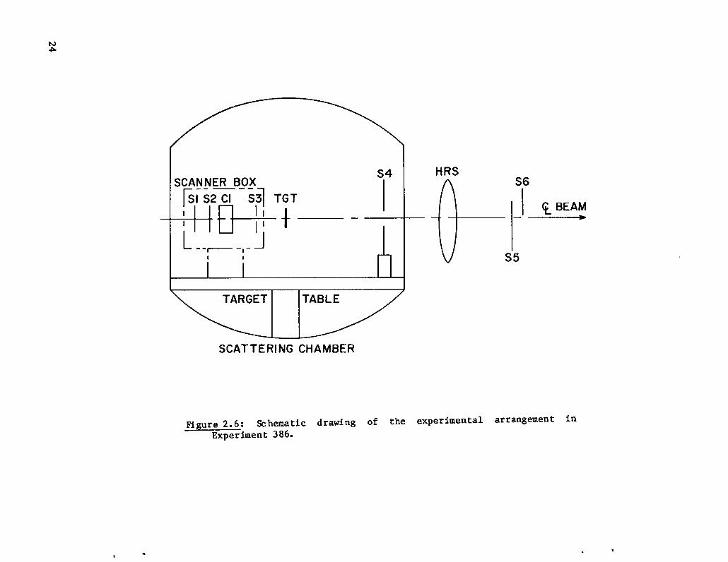
The experimental arrangement is shown in Figure 2.6. Two .010”
thick scintillation counters upstream of the target, S1 and S2, counted
the beam particles incident on the target. S3 was a scintillator of
1the same thickness, with a — “ hole drilled in it which served as a
8
veto for the beam halo. A small drift chamber, Cl, acted as a beam
profile monitor. The construction and operation of this chamber is
described in Appendix B. S4 was a veto counter located 27.63”
downstream of the target with a 1“ hole, defining a solid angle of
1.03 msr. With the HRS set at 0°, S5 and S6 were mounted on the focal
plane to intercept 800 MeV protons scattered inside the 1.03 msr veto
counter. The two focal plane counters were overlapped as shown, and
the HRS fields were set to put the 800 MeV peak just below the overlap
region. Thus S5 intercepted transmitted beau particles and the
straggling tail down to - 3.5 MeV loss.
A certain fraction of the beam was scattered outside the region
of acceptance (defined by the 1“ hole in S4) by the upstream counters
as well as by the target. Consequently target-in runs were compared to
target-out runs to determine the scattering by the target alone. h t
due to the sensitivity of the absolute measurement to systematic
effects, the time between target-in and target-out had to be kept to a
minimum. For this and other reasons the CAMAC electronics modules were
23
u
C9
I
coI
mCn
I
l-’C9+
‘1IL m.
-—1
xl
u)
:1I.-—I
=G
1,1
-1
!~-—
1-
T
I
gls--l
24.J
w08JJ
r
24
.
used to change the target configuration every 60 seconds. (Actually
the cycle time was chosen at the beginning of each run, but 60 seconds
was eventually used as a standard.) A FORTRAN program was written to
accumulate various logical combinations of the counter pulses (see
below) for a given time, then cease acquisition while the target
rotated out of the bean. While the target wheel was moving,
accumulated data were written to disk and the CAllAC scalers were
cleared. When the target reached its “full out” position, a bit was
set in the CNIAC electronics, which had the effect of stopping the
target rotation and re-starting the accumulation of data. At the end
of the next time period data acquisition again ceased, accumulated data
were written as “target-out” data, and the target was rotated back to
“full in”. So any systematic fluctuations in beam quality or intensity
were averaged between target-in and target-out. Further, suspect data
could be thrown out without the loss of a large body of it.
bunters S1, S2, S3, and Cl were mounted on a beam scanner
which allowed them to be moved independently of the rest of the
apparatus. These counters were optically aligned and mounted to a
common assembly, which was then attached rigidly to a beam scanner.
The scanner had a pair of stepping motors wh ch drove worm gears,1
providing linear translation of the counter assembly in the two
directions perpend~cular to the beam. The stepping motors were
controlled from inside CCH, and positional readout was supplied there
via sliding potentiometers on the scanner. ‘Ihusthe upstream counter
25
set could be moved independently and reproducibly up-down and
left-right to locate the beam.
In order to accurately extract the total reaction cross section
frcm the attenuation measured in the experiment, it was necessary to
know the precise angular span of the S4 veto. As seen in Figure 2.7,
for a point beam profile one may assune that all particles scattered
outside an angle 0 are not counted, and those scattered inside tJ are
counted. A beam of finite extent, d in Figure 2.7, complicates this
assumption: some particles inside e> (but outside b) are counted, and
some particles outside 0< (but inside 0) are not counted. ‘Iherefore
the spatial extent of the beam was critical to the accuracy of the
experiment.
The Line C beam optics were tuned to provide a minimally
dispersed beam on the target. Once a good tune of Line C was obtained,
a phosphor target was put in the scattering chamber and the beam was
visually steered onto the crosshairs on the target. tillimator jaws
CL04 and CL05 (see Figure 2.1) were used to cut the size of the bean
down to less than 1 mm sqare, then an upstream jaw, CLO1, was adjusted
to cut the beam current down to a countable level. With CL04 and CL05
fixed at a small aperture, drifting in the upstream magnets did not
affect the size or location of the beam on the target. ‘Iliebeam
profile was then measured by taking a drift time spectrum in Cl, and
was found to be gaussian in shape with - 0.5 mm FWH1l. l’hebeam profile
was checked periodically with Cl.
.
.
.
26

..
II
I
II
ot-
W>zcd
’
II
-f+--~
II
II
‘Iv
.2ucda02!u‘%.aJo
Uu
.I-4
,..

A similar source of error in the determination of the solid
ang1e can arise if the beam does not travel precisely through the
centers of S3 and S4. These counters were centered in the following
way: Both S4 and the scanner box containing S1, S2, S3, and Cl were
mounted on the target table in the scattering chamber. ‘Ibistable can
be rotated from inside CCH, with its angular position relative to some
arbitrary reference indicated on a digital readout. With the scanner
box lowered below the beam, the target table was rotated left until the
beam hit the right edge of the hole in S4. The process was reversed to
locate the left edge of the hole. The two values of the table’s
angular position were averaged and the table was moved to that angle.
Line C Steering Magnet 6Y (see Figure 2.1) was used to bend the beam
vertically, and the currents through the magnet corresponding to the
top and bottom of the hole were recorded. The mean of these values
located the beam at the center of S4. With the target table and
LC-S116Y set to their proper values, the scanner box was moved up-down,
and right-left to center the hole in S3 about the beam. l’husthe line
defined by the centers of the two holes was colinear with the beam.
A schematic diagram of the electronics used in the experiment
is shown in Figure 2.8. Signals from all scintillators were first
discriminated in either Lecroy Research Systems Model 621 or 821
leading edge discriminators. Thresholds were set to - 30 nv and output
pulse widths set to 10 ns. %xue outputs from these units were further
discriminated so their output pulses could be independently widened for
use as vetoes in logic units. For example, an output from the S3
.
.
.
.
28

..
l--r
II
n.y(J(
7-
c*rnu%-lc0kvaJ
?-4auw-l
5’
29

discriminator was fed again to a LRS 821 where its output width was set
to 40 ns and used as a veto into the LRS 365ALP to give Sl*~. h
output of this unit was fed to a LRS 322A coincidence register along
.
.
with the discriminated output of S2 to give S1 “S2‘S3, or BEAM. The
discriminated output of S4 was similarly widened and used as a veto to
BEAM in aLRS 364AL. Then BEAM*~was joined with the discriminated S5
signal to form BEAll*=*S5, or EVENT. As their names imply, BEAM
represented those protons incident on the target, and EVENT represented
BEAM particles which scattered inside the 1“ hole in S4 and were
transmitted through the HRS to S5.
As in any coincidence measurement the possibility exists to
count a “true” coincidence (e.g. a beam particle) when in fact an
“accidental” coincidence (e.g. two unrelated cosmic rays) has occured.
These accidentals are assuned to be uncorrelated in time, SO by
delaying one of the coincident pair one gets a measure of the
probability of accidental overlap of the two signals, i.e.
A-B = true
A-did B = accidental .
However if one knows (or suspects) that most of the singles in either
counter come from true coincidences, the above method will overestimate
the rate of accidentals. In this case the measure of the nunber of
accidentals should be restricted, specifically how many events are
counted as coincidences that are not true coincidences. This may be——
.
30

accomplished by forming A“% and forming a coincidence between this and
a delayed signal from B:
(A*~)”dld B = accidental .
This was the situation in Experiment 386, so accidentals were
dealt with in this way. The discriminated signal frou S1 was widened
to 40 ns and used as a veto to the discriminated signal of S2 in a
LRS 465 logic unit. The output of that unit, =“s2, was thus
guaranteed not to be a beam particle. lhis signal was delayed and fed
to a LRS 322 coincidence unit with Sl*~. The output of that unit was
BEAllACCIDENTALS. Similarly to form EVENT ACCIDENTALS, part of the
definition of EVENT, BEAM”S4, was widened and used as a veto to the
rest of the definition, S5, yielding an S5 event corresponding to no
BEAM particle. This signal formed a coincidence with a delayed BEAli*S4
signal in a LRS 365AL to give EVENT ACCIDENTALS. Accidental
coincidences between
last quantity gave a
by S4.
S4 and BENI were formed in a similar manner. This
measure of the accidental vetoing of a good EVENT
obst of the information described here was scaled, noted S on
the electronic diagram. The outputs of these various modules were
-1.7 v pulses which were connected to 12-channel CAMAC 24-bit scalers.
At the end of each “target-in”. and “target-out” cycle the accumulated
counts in these units was written to disk via the FORTRAN program
EXP386, and the scalers were cleared.
31

CHAPTER III
ANALYSIS OF THE DATA—— —
A. EXPERIMENT 470: REACTIVE CONTENT OF THE OPTICAL POTENTIAL
The off-line analysis of the data from Experiment 470 was done
(19,20)using the standard HRS data acquisition system “Q” in a “Must
Process” mode. This system consists of three major components: an
ANALYZER, a DISPLAY package, and an ALLTEST package. The ANALYLI%K is
primarily responsible for converting the 38 taped words containing time
and pulseheight information into physical quantities such as
(xf, ef,yf,~f) and (6t,qt,yt, d). The ANALYZER also calls a relativistic
kinematics subroutine KINREL to correct for the recoil of the target
nucleus, arriving at the Missing Mass. Of course these quantities are
complicated functions of times and pulse heights, so in the process of
calculating them many other intermediate quantities are also
calculated. In all the ANALTLER generates over 200 DAi’AWORDS which
can be displayed or used in the ALLTEST package.
DSP(21)The DISPLAY package, > permits the creation of
one-dimensional histograms, the entry, retrieval and plotting of these
histograms, and the dynamical display of two-dimensional scatter plots
as data are acquired. The user can specify which DATA WORD is to be
plotted, a test to be passed for entry to the histogram, and display
parameters. L)SP is therefore closely linked to the ANALYZER and to
ALLTEST. In addition one may use cursors on displayed data to define
.
.
.
32

.
the limits of GATES and BOXES, which are in turn written as tests to
the ALLTEST package.
ALLTEST is a subroutine to the ANALYZER which allows the user
to perform tests on raw and calculated DATA WOKDS (MICROTESTS) or on
logical combinations of previous tests (MACROTESTS). A MICRO’ILST
specifies a bit pattern or upper/lower limits on the value of a DATA
WORD (including the limits defined in GATE and BOX commands to
displayed data ). A MACROTEST specifies logical combinations of
previous MICR& or MACR&TESTS or their complement (AND, OR, EXCLUSIVE
OR). Tests are defined in the Test Descriptor File (see Appendix C)
which is written in a clear and concise format to facilitate the
evolution of off-line replay of the experiment. Through the Test File
one can easily tighten or loosen the definition of a “good” event,
define a restricted region of the focal plane, or change Particle
Identification limits. The Test File for Experiment 470 was used to
count protons scattered into a solid angle W and monentum interval hp
(Test 76) to arrive at the double-differential cross section. Other
tests were used to determine the focal plane efficiency, software
efficiency, and normalization of the data.
Al: The Differential Cross Section
In scattering experiments the number of particles scattered
into a solid angle AQ is proportional to the beam flux, the size of ~~1~
and the number of scatterers intercepting the beam:
33

dN = o(e)”N “AU*nb s“
(3.1)
.
The constant of proportionality u(0) is the differential cross section
and
u(6)*A$1= do(d) (3.2)
so that
For elastic
the quantity
~= dN. (3.3)
dS1‘b”ns”Ab2
and inelastic scattering to discrete final states this is
of interest, and beam particles which leave the nucleus in
discrete states are easily identified and couuted with a spectrometer
such as the HKS. However scattering to the continuum does not result
in outgoing protons with discrete energy losses. In this region the
scattering yield into a solid angle Ailand momentum interval Ap is
(3.4)dN = a(O,p)”Nb ”n~”Af~”*P ,
and by analogy with Equation 3.2
IJ(e,p)”A~)”hp= d%(~,p) (3.5)
.
.
.
so that the quantity of interest is
34

.dzd~, p) = dN
dktdp Nb .n~.Afj.A~ “(3.6)
.
Determination of the right side is the object of the experiment.
A.2: NORMALIZATION
Since the (p,p’) inelastic spectra for excitations greater than
about 160 MeV are structureless over the momentum acceptance of the tiKS
(~ = tl.2 %), and because the angle-integrated (p,p’) cross sections
daare
%structureless over the solid-angle acceptance of the iiRS
(AO = ~ 1° in the plane of scattering), the full phase space acceptance
of the HRS was used for each HltSangle-field setting to generate a
d ‘Osingle data point for the relative —.
dfklp
However the momentum-solid angle, acceptance function of the
spectrometer is not uniform over the entire focal plane, so that a
technique had to be devised to obtain the absolute cross sections.
This technique, described below, involved using a small region at the
center of the focal plane, where the acceptance is uniform, to
the d~ocross-normalize some of data to ‘H (p,p) elastic scattering
dikip
data obtained during the course of the experiment. Since the elsastic
1H (p,p) cross sections are known,
d‘uthe absolute cross sections for —
dkklp
were
Then
with
easily obtained for the restricted angle-momentum acceptance runs.
d ‘uit was simply a matter of scaling the relative— data obtained
ditip
the full acceptance, to obtain the absolute cross sections.
35
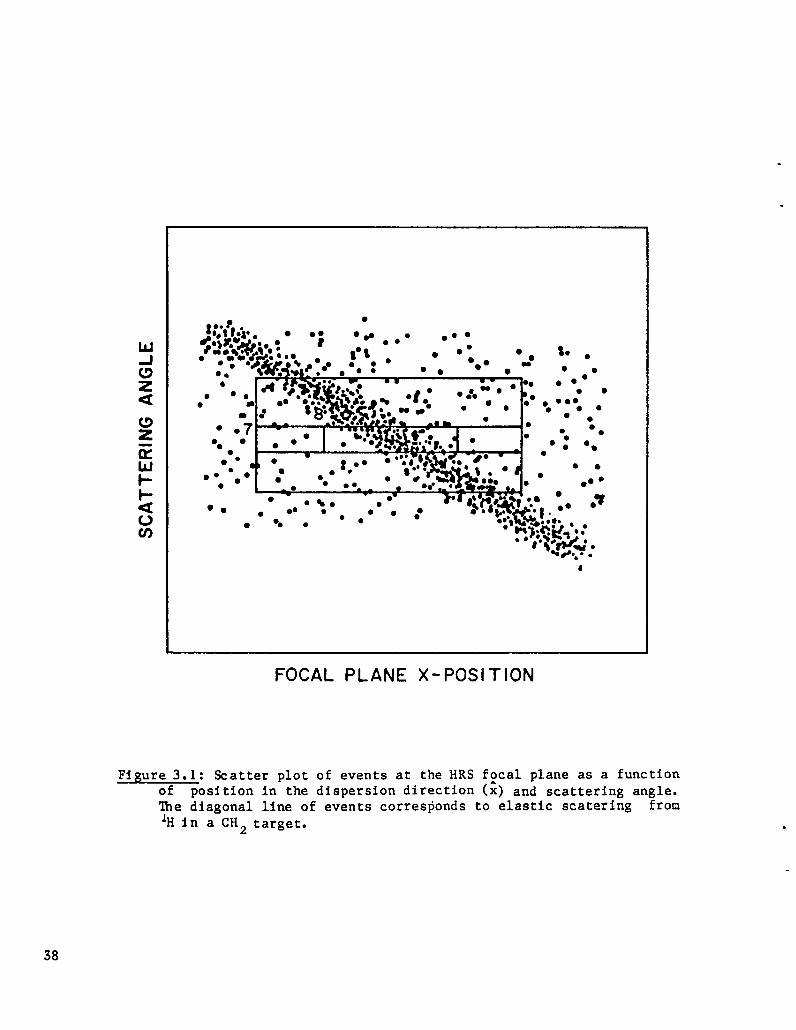
Figure 3.1, obtained using a CH~ target with the HRS at 15° and
fields set for ‘H (p,p) elastic scattering, shows a scatter plot of
events at the focal plane as a function of dispersion coordinate and
scattering angle. The diagonal line of events corresponds to protons
1elastically scattered from the H in the CH2. The angle-position
correlation is due to the large kinematical% ( -9.4 14eV/deg) at this
angle. Eox 7 in the figure was used as a test to constrain the
scattering angle to the central 0.3° accepted by the HRS. Because of
the largedE
x’Box 7 also effectively restricts the focal plane
dispersion coordinate to t 2.1 cm (the focal plane is 60 cm in this
direction). The lH (p,p) events passing the Box 7 test occur over a
central region of the focal plane (- 0.7 % of the full acceptance) for
which the relative momentum-solid angle acceptance is known to be
9uniform.
For ‘H (p,p) elastic scattering we have
du(~) = K*NB7~cF
dfl IC .ns(3.7)
where NB7 is the number of counts in 80X 7, CF accounts for the
efficiencies of the drift chambers relative to the event trigger, IC is
a relative current monitor, and ns is the areal density of scattering
centers in the target. Thus the normalization constant K accounts for
the gain of the ion chamber, the overall trigger efficiency, and the
size of AU defined by Box 7. Since ~ for 800 MeV ‘H (p,p) elastic
(22)scattering is known , K can be calculated.
.
.
.
36

i
d ‘aIn order to obtain an absolute normalization for the — data,
d&tip
Box 8 (Figure 3.1) was used in the test file to define the same angle
limits as Box 7, but a dispersion direction region corresponding to the
region indirectly defined by Box 7 for the ‘H (p,p) data. Since the
trajectory’s dispersion coordinate on the center of the focal plane is
linear with dispersion
Ap PO-PSP‘f =U*6=I)*-=D*
P3
Psp
(3.8)
where D is the dispersion, Psp is the momentum corresponding to
optic axis for given HRS field settings, and p. is the momentum of
trajectory. Therefore
PspAPBOX8 =
“%0 x8D
s (3.9)
the
the
so that
d20 _ K*D . NB8 ●CF
d$tip‘BOX8
IC*ns.p ‘Sp
(3.1(J)
where NB8 is the number of counts in Box 8. Since K is known from the
1H (p,p) analysis, absolute double-differential cross sections were
obtained. l-bweverBox 8 selects only a small fraction of the events
detected at the focal plane, so the absolute normalization runs were
37
●✎☛
.00
●●
● m ●
● “ ●e .● @
09°●“%“ee@
fee ● .@*-* 6.00
- ** ●
●●.-
i?
● ✎
b-
1
● . #-/#●
● ml”
● ●-7+ - l-”=
h ●
● ●●
✎☛
● o● ● 00● ● 0
● 0
● .
● S ●
1
● .●
● ●. . .●0 ●
FOCAL PLANE X-POSITION
Figure 3.1: Scatter plot of events at the HRS f~cal plane as a functionof position in the dispersion direction (x) and scattering angle.‘he diagonal line of events corresponds to elastic scatering fron‘H in a CH2 target. .

.
considerably longer than those runs for,,
d‘awas used to obtain the relative —.
dkkip
Box 9, shown in Figure 3.2,
which most of the focal plane
was used to obtain the relative
doubledifferential cross sections for all of the runs. As stated
d ‘uearlier, — is a smooth function of both momentum and angle, and
dS&lp
varies little over the momentum- and solid angle-acceptance of the HRS,
so that a factor A can be used to cross-normalize the Box 9 derived
relative cross sections to the Box 8 derived absolute cross sections
obtained from the normalization runs:
NB9 “CF KoDA*K— =
NB8 ●CF.IC*ns ●p
Sp ‘Bo X8IC*ns*p “Sp
Thus
NB8A==-
D.
‘Box8
(3.11)
(3.12)
These Box8 - BOXY normalization runs were made in the region
800 MeV/c < psp < 1000 MeC/c where the cross section is smoothest. The
results for several angles and targets were statistically averaged.
d 20The final expression to be used in calculating—
d~kipis then
d20 _ A*K*NB3”CF
dikip IC*ns.p ●
Sp
(3.13)
39
—

FOCAL PLANE X-POSITION
Figure 3.2: See Figure 3.1. These data were taken at energy-losscorresponding to pion production. tixes 7, 8, and 9 are discussedin the text.
.
I ● I
.
.

.
.
The HRS acceptance is a function of beam-on-target width in the
non-dispersion direction. For thin targets the region of uniform
acceptance is about z ~ cm in the direction transverse to the optic
axis of the HRS. Since the beam-on-target width is typically less than
?+ cm, no problems are encountered.
kwever for the 5 cm cylindrical LH2 target used during
Cycle 25, the beam-target volume was 5 cm long in the beam direction,
so that the “effective” target thickness seen by the HRS (Figure 3.3)
1varied with spectrometer angle. Therefore during the LHZ runs H (p,p)
elastic were also taken at each angle using a solid CH2 target, and the
normalization of this solid-target data made it possible to account for
the variation in the effective target thickness of the liquid-target
data. The CH2 data were normalized using the BOX 7 technique described
above.
Finally it is to be noted that the IC gain was different for
the two running cycles. Since normalization data using the CH2 target
were obtained for both Cycles 25 and 26, the different ion chamber
gains presented no problem. As a further check of the normalization
2(J8elastic scattering data were taken for p + Pb at blab = 5° during
(23)Cycle 26, and compared to the data of iioffmann et al . The two——
normalizations thus got agreed to within 2 X.
41

U)
axml
x-
-J0.-Wd.-CN
II=
’aumd
..
Ii
..
42
.
.
A.3 BACKGROUNDS
The scheme
pure target. In
outlined above assunes that the scattering is from a
fact, however, protons scattered from impurities in
the targets, Helium in the scattering chamber, and the LH~ target flask
were also detected. It was necessary to subtract such events from the
data in order to arrive at meaningful results. Further, extraction of
1H (p,p’) inelastic information from data obtained using the CHZ target
12required that scattering from C be accounted for.
For all targets,
measurements were made to
the LH2 runs the background
For the solid-target data
including LH~, target-in and target-out
determine the background contribution. ?0r
due to the Mylar flask was typically 5 X.
obtained during Cycle 25, the Helium in the
scattering chamber contributed between 3 X and 20 Z to the total yield.
Background during Cycle 26 were typically 5 Z.
Extraction of
sections was a similar
1the H (p,p’) cross sections from Ctizcross
exercise:
I*=( ‘BY”CF)* + INB9”CF I*
where the * indicates that backgrounds have been subtracted.
(3.14)
Then
(3.15)
43

40One more adjustment to the Ca data was made. Figure 3.4 is a
spectrum of protons elastically scattered from the ‘°Ca target at 5°.
The second peak seen corresponds to protons elastically scattered from
a lighter nucleus, in this case an ’60 contaminant. Since data were
not taken on ’60, no definitive number was available to be subtracted,
so the assumption was made that
based on total reaction cross section measurements. ‘Ihen
d 2U(—J
d 2a—)= 1.21 [dh~ dp 1~~ ‘
d$ldp 160
(3.16)
(3.17)
and the 40Ca data were adjusted accordingly.
A.4: Uncertainties
Aside from statistical uncertainties in the data and
backgrounds, there are three sources of uncertainties in the results:
target thickness, the derivation of A in Equation 3.12, and overall
normalization of the data.
‘i’hetarget thicknesses were known to 2 X, and this error is
included as an uncertainty in ns.
.
.
.

.
b
oo—(9
O“
—*
—0
(~JD
J+!qJD
)slNno~
.
45

‘he error in the determination of A by Equation 3.12 is
By calculating A for different angles and targets,
errors) were obtained and statistically averaged.
(3.18)
several values (with
The distribution of
A’s had a ~’ of 0.7, so calculation of the errors by purely statistical
means may have overestimated them slightly. These quantities were
nonetheless used in the
The assumption
Alinear in xf, does have
reported results.
that generates Equation 3.8, namely that b iS
some inherent error, but these higher order
terms in 6 are -J0.4 % and so were ignored.
Apart from the above uncertainties, the uncertainty in the
overall normalization of the data depends on the uncertainty associated
with the data used to determine the absolute normalization. Both the
800 MeVp+pandp+208
Pb elastic data used for
have quoted uncertainties of 5 %.
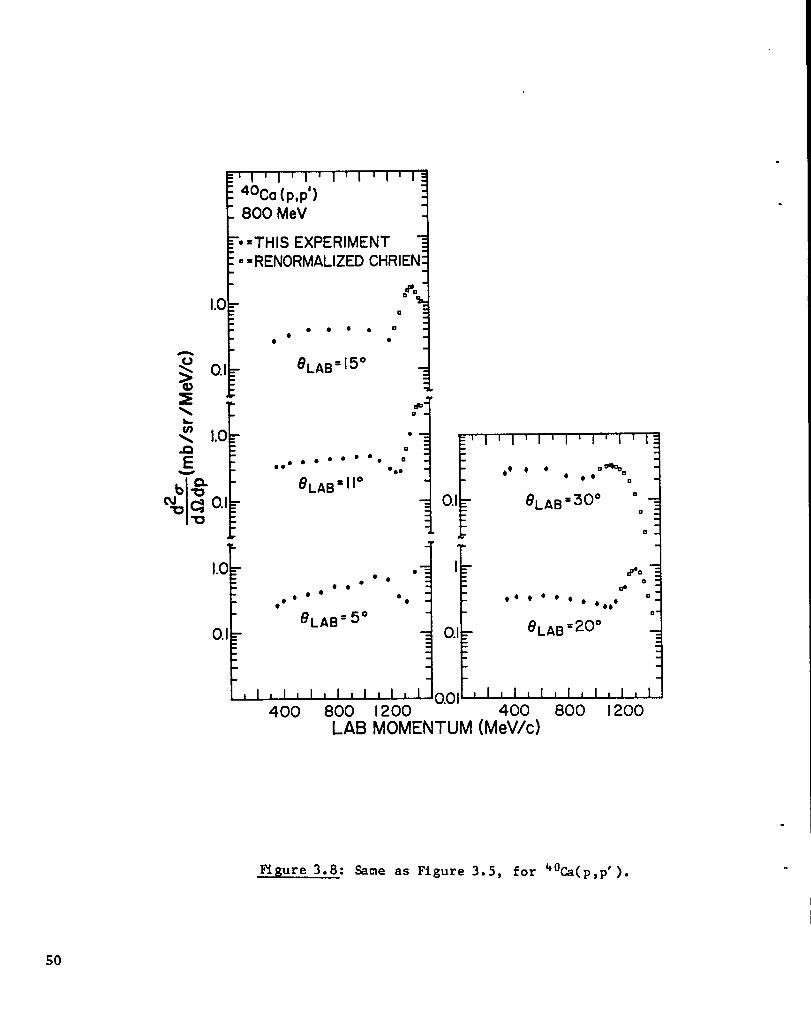
A.5: RESULTS
The results of the experiment are
in Appendix A. Also shown in the figures
shown in
are the
this normalization
Figures 3.5-3.9, and
(renormalized) data
of Chrien, et al(24) for the quasi-elastic region..— The data obtained
in this experiment and the Chrien data have absolute normalizations
which differ by from 11 % to 25 %, depending on target and’angle. .
.

.
0.1
I0.01
~’I’’’l ’’’l’”q ~“’’’’’’’’””~
? 0.1F
J 0.01=
0.01
I1-
‘H(p,p’)800 MeV
● 9.● 9,9
●
● **‘“ 8~A~=150
b
●
e**
e
0LAB=5”++
b
I
* It
L
!1.00
--
.01
.001
*+* ● ●
9LAB =30°
?
*
E .001:
Llllllll,l,lll ll;‘,,,,,,,,,,,,,,,400 800 1200 400 800 1200
LAB MOMENTUM (MeV/c)
.
Figure 3.5: ‘Itie double-differential inclusive cross section for‘H(p,p’) scattering at 800 MeV.
47
p“’’’’’’’””q2H(P,P’)800 MeV
1.0:
0.1~ 004c
●
a
0.1
[
0.01
1
6e *
++++
6LAB=30”*
6 0~++
8LAB=II” $+
1[0.01
,*** ● 0.1~
*** +
** ‘+
8LAB=5” ~ 0.01-
I I 1 I I I I I 1 I I I 1 I 1 I 1 I I I I I I I I I
400 800 1200 400 800 I200LAB MOMENTUM (MeV/C)
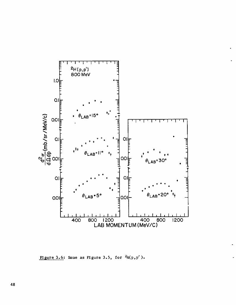
Figure 3.6: Sane as Figure 3.5, for 2H(p,p’).
*.me
● “ +*
*8LABX20” *++ (
.
.
.
.
.
& *F
11.0 u0.1L -1 1-
o●n●
❑ m. ● * ● ● ●,,* o,*
8LAB=200/
t
0.1 .“ “
“-4 k
0.018~AB= 5°
o.o,L_lA_uJlLu_w_dJ400 800 1200 400 800 1200
LAB MOMENTUM (MeV/c)
I I I I 1 I I I 1 I I I I I
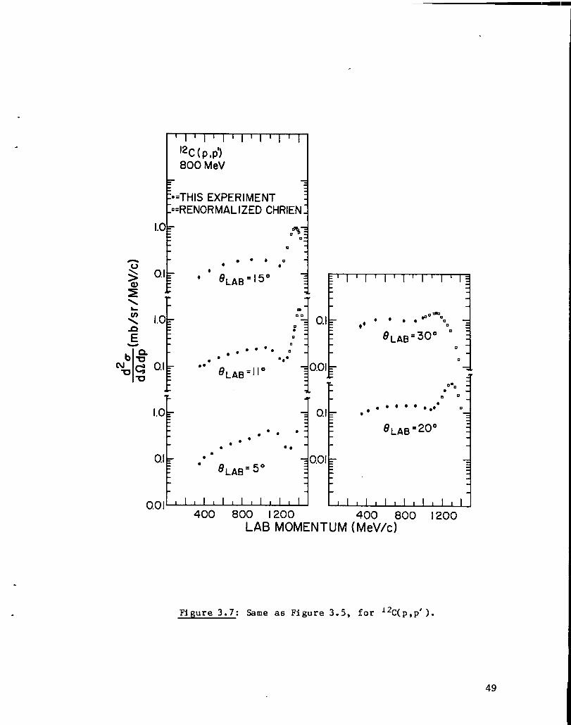
‘*c(p,p’)800 MeV
:D=THIS EXPERIMENT.LI=RENORMALIZED CHRIEN.
t-
* 0 0~A~=i50i :“’’’’’’’’’’”2
\ :
“ 0.1:0
❑
● *..● “”.0 ..*
“0 8~AB=llo 0.01
‘F
Figure 3.7: Same as Figure 3.5, for 12C(p,p’).
49
F●XTHIS EXPERIMENT
{.xRENORMALIZED CHRIEN
●● “
***,,*
8LAB=5”
●
!$%
00
●
1’9
HI
● *
●*
0.1
-1
Illllll,llllld 00,LJALLUJ400 800 1200 “ 400 800 1200
LAB MOMENTUM (MeV/c)
Ngure 3.8: Same as Figure 3.5, for ‘°Ca(p,p’).
50

.
IN
7
m10
I
●=THIS EXPERIMENT
4==RENORfVIALIZEDCHRIEN
I.0*
. t
● ☛ ● 9*.**
6’*~=110
●“ .,, ***
8’A~ =5°
●O
●
I#09
0..9°
●
●
●
●
/
E“’’’’’’’’’’”a
1.0~ +**,* * ,0-%
OLAEI=SO” “0
1
0
01
Lo
0.1r
I I I I 1 I I 1 I I I I 1 I I 1 I I I I I I I ! I I I I I I400 800 1200 400 800 1200
LAB MOMENTUIVI (MeV/c)
I1.0
0.1
**,●☛☛✌✌
OLAB=20”
Figure 3.9: Same as Figure 3.5, for 20bPb(p;p’).
51

B: EXPERIMENT 386: TOTAL REACTION CROSS SECTIONS— .
B.1: The Attenuation Cross Section——
In the off-line analysis of the Experiment 336 data the
attenuation cross section was calculated from the recorded data, and
reaction cross sections were calculated from the attenuation cross
sections. The attenuation of a particle beam by a target of density P
is described by
N = No” e-pm , (3.19)
where No is the number of beam particles, N is the number of particles
transmitted through the target, x is the target thickness, and u is tile
attenuation cross section. This experiment was performed with counters
upstream of the target, and they scattered - 0.3% of the beam. In fact
those counters scattered a fraction of the beam that was on the order
of the fraction scattered by the targets. Denoting i..and i as the
beam and transmitted particles, respectively, with no target in the
beam; and Ioand I as those quantities with the target in the beam
i -Pcucxc ,= ioe (3.20)
‘(PC~CxC + pA”AxA) ,I = Ioe (3.21)
where the subscript A refers to the target nucleus, and c to the
counters. lhen the attenuation cross section due only to the target is
.
52
●
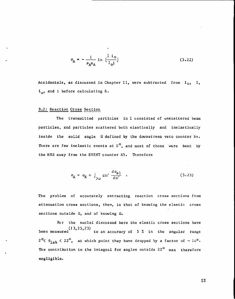
1 I i.GA = -— in [—j
pAxA I~i(3.22)
Accidentals, as discussed in Chapter II, were subtracted from l., I,
i~, and i before calculating S.
B.2: Reaction Cross Section
The transmitted particles in I consisted of unscattered beam
particles, and particles scattered both elastically and inelastically
inside the solid angle S2defined by the downstream veto counter S4.
There are few inelastic events at 0°, and most of those were bent by
the HRS away frcm the EVENT counter S5. Therefore
(3.23)
The problem of accurately extracting reaction cross sections from
attenuation cross sections, then, is that of knowing the elastic cross
sections outside Q, and of knowing Q.
For the nuclei discussed here the elastic cross sections have
(13,25,23)been measured to an accuracy of 5 % in the angular range
20< elab < 22°, at which point they have dropped by a factor of - ll)b.
The contribution to the integral for angles outside 22° was therefore
negligible.
53

‘Ihe veto counter S4 defined ‘anazimuthal angle of - 1°, so
there remained a small region inside 2° for which the elastic cross
section had to be calculated. The Optical Model fitting routine
IwoMN(2’) was used to calculate that cross section for 1°< ~~ab <2”.
The calculated cross sections were constrained to fit the data for
2° < 6 <10°, and since the 6 < 2° region is dominated by ~ulo~b
scattering, the calculated values were considered more than sufficient.
B.3: Systematic Errors and Corrections
One uust consider three possible corrections to the extraction
of reaction cross sections as oulined in the scheme above: inelastic
transmitted to the EVENT counter S5, straggling, and Multiple Coulomb
Scattering. The contribution made by these processes to the reaction
cross section will be discussed here. Further, possible sources of
error associated with the uncertainty in the measurement of ~1,
uncertainties in the known elastic cross sections, and statistical
uncertainties will also be discussed.
B.3a Forward Inelastic: The correction due to forward-scattered
inelastic events was negligible. One has to consider only protons
scattered at angles less than 1° to states of Ex < 3.5 ~leV in the
target nucleus: in ‘o& the (0+,3.35); and in 208Pb the (3-,2.61) and
(5-,3.20).(13,27)
Data for these reactions are available only for
angles greater than - 4°, so estimating their contribution for the
range 0°< 0 <1° by the cross section at 4°, one obtains values less
.
.
.
.
54

than 0.1 mb, or a contribution to the reaction cross section of around
one part in 104.
B.3b Straggling: The straggling of the beam in both the upstream
counters and in the target can cause a fraction of the transmitted beam
to miss the EVENT detector S5; i.e. those particles degraded by more
than - 3.5 MeV will be bent by the HRS away from S5. Of course,
straggling will not affect the counted BEAM, 10 and io, so denoting the
measured quantities with primes,
I = 1’ + Istrgl
i = i’ + istrgl
(3.24)
(3.25)
where Istrgl (i5trgl) is the portion of the transmitted beam not
counted due to straggling in S1, S2, and the target (S1 and S2 only).
Since pox is small ( <.01 ), Equation (3.22) can be written
where
‘= (+-:1o 0
Then
(3.26)
(3.27)
55

.L[s’+kd’yj ●
‘A ~x i. o
(3.28)
With no target in the beam the fraction lost, cs~ iS due onlY to to the
scintillators S1 and S2
‘strgl = csio , (3.2!4)
and with the target in the beam the fraction lost is due to both the
scintillators S1 and S2 (c’) and to the target (ct)
lstrgl = (c’+ ct)Io ●
So Equation 3.28 becomes
aA .: (s’ - Ct)
and the fractional error in aA due to straggling loss is
~aA Ct—=—e
“As
(3.30)
(3.31)
(3.32)
Calculations of the straggling tail to energy losses greater
than about 3.5 MeV were made using the program LANDAU, based on the
(28)theory of Vavilov . An uncertainty of 35 mb was calculated for the
208Pb target. For the other targets%< .01 .
.
.
.
56
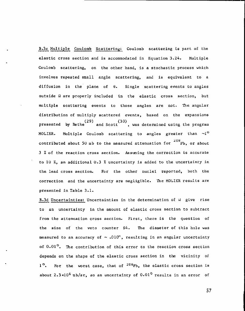
. B.3c Multiple Coulomb Scattering: Coulomb
elastic cross section and is accommodated in
Coulomb scattering, on the other hand, is
involves repeated small angle scattering,
scattering is part of the
Equation 3.24. Multiple
a stochastic process which
and is equivalent to a
diffusion in the’ plane of 6. Single scattering events to an@es
outside Q are properly included in the elastic cross section, but
multiple scattering events to those angles are not. The angular
distribution of multiply scattered events, based on the expansions
presented by Bethe(29)
and Scot~30) , was determined using the program
MOLIER. Multiple Coulomb scattering to angles greater than -~o
ZU8contributed about 50 mb to the measured attenuation for Pb, or about
3 2 of the reaction cross section. Assmning the correction is accurate
to 1(I%, an additional 0.3 % uncertainty is added to the uncertainty in
the lead cross section. For the other nuclei reported, both the
correction and the uncertainty are negligible. The MO”LIERresults are
presented in Table 3.1.
B.3d Uncertainties: Uncertainties in the determination of kt give rise
to an uncertainty in the amount of elastic cross section to subtract
from the attenuation cross section. First, there is the question of
the size of the veto counter S4. The diameter of this hole was
measured to an accuracy of - .010”, resulting in an angular uncertainty
of O.O1°. ‘he contribution of this error to the reaction cross section
depends on the shape of the elastic cross section in the vicinity of
10. For the worst case, that of ~08pb, the elastic cross section is
about 2.3x10⁶ mb/sr, so an uncertainty of O.O1° results in an error of
57

t 30 mb. A second source of error due to ktis the position of the bean
relative to the center of the hole in s4. The process of locating the
center of that hole was carried out twice, about 48 hours apart, and
the results were repeated exactly. Since the position was read to
~ 0.010, it seems safe to assume that this location was known to
*0.030.s such an error contributes less than 10 mb to the integral of
the elastic cross section for 208Pb, less for the other nuclei.
Target thicknesses were assumed accurate to 2 Z.
Another source of error in the extraction of the reaction cross
(13,25,23)sections is the error in the known elastic cross sections .
Error bars on these data are - 5%, and contribute to the reaction cross
sections differently for different nuclei. For example, there is an
‘k reaction cross section of N 5 mb due touncertainty in the the 5%
error in the elastic, whereas the 5% translates to -130 ub in 20bPb.
From the expression 3.22 for GA statistical uncertainties are
1 Ioi I i.6aA = ——*6 [—J ●PX I i. Ioi
(3.33)
The statistical uncertainty of the quantity in parentheses results
entirely from 61 and 6i, since 10 and i. measure the beam, whereas I
and i represent, to some accuracy, the effect of a probabilistic
process on the beam. lhen
(3.34)
58

Finally with
61= [1(1 -:) 1+o
one has
(3.35)
(3.36)
(3.37)
From this final expression it can be seen that the scattering by the
upstream detectors contributes to the uncertainty on an equal footing
with the scattering by the target, indicating the advisibility of using
the thinnest possible BEAM counters. (Note the expressions (3.35) and
(3.36) seem somewhat different from those commonly used in scattering
experiments. The apparent difference arises from an approximation
normally employed to reduce a Binomial distribution to a poisson
distribution(31)
, so that AN = h. The assumption in the approximation
is that the probability deduced is small. Such is not the case in a
transmission experiment, since ~ --1.)10
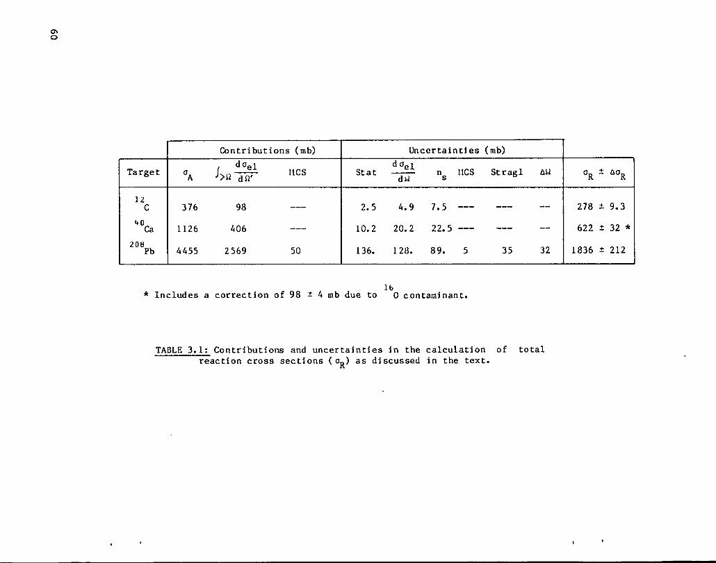
B.4: RESULTS
The extracted total reaction cross sections and various
contributions to their errors are presented in Table 3.1.
59
In
al
uuc—sEUIco
I1IIII1Iu-l
.-mu“
u-l
.‘NIIIar+m
.
Q.i0C
iox
.“a)
4JU
tic
c1w
-!
2’%U
ul
c:.-
vm(n-
@u
.1-b-l(n
cm
aw
gul2C
m.:
Cu
CL!u
2:Oul.“
m
..

CHAPTER IV
SUMMARY AND CONCLUSIONS
The experiments described in the preceding chapters were
carried out to provide data which test the main assumption used in
practical applications of multiple scattering theory: use of the
impulse approximation. The effect of this approximation is to restrict
the allowed reaction channels to those initiated by nucleorrnucleon
collisions: nucleon knockout and quasi-free pion production. In order
to provide a basis for comparison with p+ nucleus data, a complete set
of p+p inclusive cross sections was obtained. A discussion of the
lH(p,p’) data is given in Section A. Section B presents the
p+ nucleus data, and Section C discusses the conclusions that can be
drawn from the data.
A: THE HYDROGEN SPECTRUI1—
Figure 3.5 shows the inelastic lH (p,p’) spectrum at lab angles
up to 30°. ‘Ibisspectrum corresponds almost entirely to single pion
production. At 800 MeV the process of single pion production proceeds
3primarily through the p-wave resonance A~~ (J = —, T =
2~), and has been
(33,34)explained most successfully in terms of One Pion Exchange (OPE) ●
Therefore the diagrsms assuned to contribute to the *H (p,p’) inelastic
spectrun are those shown in Figure 4.1.
(
61
.
a)i
IP P
PI
n
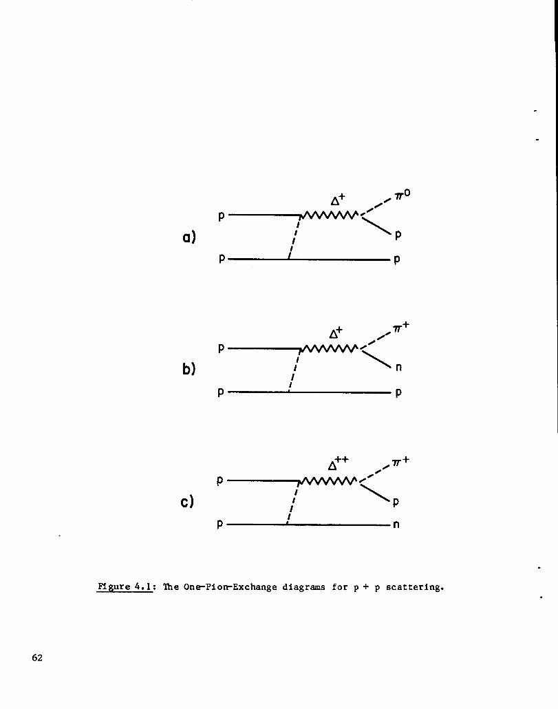
Ngure 4.1: The One-Pi omExchange diagrams for p + p scattering.
.
.
62
.
.
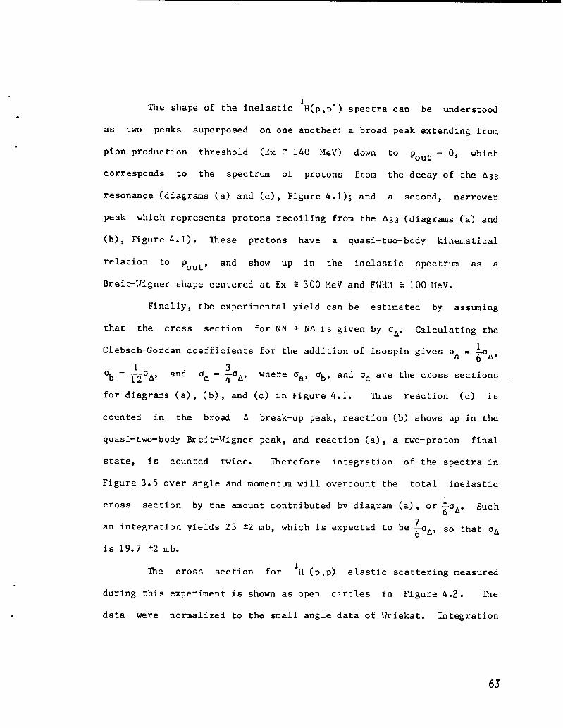
1The shape of the inelastic ~(p,p’) spectra can be understood
as two peaks superposed on one another: a broad peak extending from
pion production threshold (Ex = 140 MeV) down to Pout = 0, which
corresponds to the spectrtnn of protons from the decay of the A33
resonance (diagrams (a) and (c), Figure 4.1); and a second, narrower
peak which represents protons recoiling from the A33 (diagrams (a) and
(b), Figure 4.1). These protons have a quasi-two-body kinematical
relation to pout’ and show Up in the inelastic spectrum as a
Breit-Wigner shape centered at Ex z 300 MeV and
Finally, the experimental yield can be
that the cross section for NN + NA is given
ClebsckGordan coefficients for the addition of
FWHI1 = 100 lleV.
estimated by assuning
by OA. Calculating the
1isospin gives csa = g~~,
1 3‘b ‘@A’ and UC = —u4 A’ where aa, ab, and ac are the cross sections
for diagrams (a), (b), and (c) in Figure 4.1. IIIus reaction (c) is
counted in the broad A break-up peak, reaction (b) shows up in the
quasi-two-body Breit-Wigner peak, and reaction (a), a two-proton final
state, is counted twice. Therefore integration of the spectra in
Figure 3.5 over angle and momentun will overcount the total inelastic
cross section
an integration
is 19.7 *2 mb.
by the amount contributed by diagram (a), or~uA. Such
yields 23 *2 mb, which is expected to be la6 As SO that uA
The cross section for ‘H (p,p) elastic scattering measured
during this experiment is shown as open circles in Figure 4.,2. me
data were normalized to the small angle data of Wriekat. Integration

160
140
I20
I00-:\
2- 80
eu>u
6C
4C
2C
c
lWP, P’) 800 MeV
● = INELASTICO = ELASTIC THIS WORK❑ = ELASTIC, wRIEKA~ e
.
.
8 LAB (deg).
.Figure 4$ : Angular distributions of the elastic cross section (open
circles) and the momentun-integrated inelastic cross section
(solid dots) for800MeV lH(P,P’) scattering=

.
.
of the elastic data yields oel = 25.1 t 1.2 mb. From this
interpretation one concludes that oT(p+p) = Uel + CA = 44.8 t 2.3 mb.
‘he experimental yield from a p+ n experiment can be similarly
evaluated by assuning
scattered proton in
relationship, that in
the contributing diagrams in Figure 4.3. The
diagram (a) has a quasi-two-body kinematical
diagram (c) will be counted in the broad d
break-up region, and diagram (b) will be counted twice. Diagram (d)
has no proton in the outgoing channel, so the contribution it makes to
‘A will be lost; however its ClebsclrGordan coefficient is equal to
that for diagram (b) (which is ove~counted), so the integration over
angle and momentun will yield the correct value of oA“
B: NUCLEAR INELASTIC SPECTM—
The inelastic spectra for p + nucleus scattering are shown in
Figures 3.6-3.9. . ‘he outstanding feature of the spectral
.distributions is their marked
indicating that nucleon-nucleon
p + nucleus scattering. At the
similarity to the p+p spectrum,
processes dominate highly inelastic
large momentun end of each spectrun is
a peak corresponding to quasi-elastic nucleo~nucleon scattering. This
region has been investigated at an incident proton energy of 800 MeV by
Chrien et al.(24)
.— , and their data are shown in the figures as open
squares. ‘Ihereis some discrepancy between Chrien’s normalization and
ours, as discussed in Chapter III. The points shown conform to the
normalization of this experiment.
65

.
a)
P
b)
n
P
c)
n
n
A“
~’”””/’ \
A+
~“’””/ \I
in
7T-
d)
A+~T+
P ~“”’/’ \ n1’
n n
.
.
Pigure 4.3: The OnePiorExchange diagrams for p + n scattering.

.
.
At outgoing momenta lower
spectra, the same structure can be
for p+p scattering. Because
than that of the deep minimum in the
seen for p + nucleus scattering as
of this similarity of shape and
position, these lower momentun data are assuned to be the result of
quasi-free &production. ‘he similarity between the p+ p inelastic
#spectrun and the p + nucleus highly inelastic spectra deteriorates for
.heavier nuclei: whereas the p+ ‘H data are essentially identical to
208the p+ p data (except for a scale factor), the p+ Pb data resemble
the p + p data only at small scattering angles.2oti
Indeed, for Pb at
01ab = 30° the cross section in the quasi-free A region increases
monotonically with decreasing pout. Such behavior with increasing A
and ‘lab is to be expected, since the effect of the nuclear medium on
the outgoing proton grows with nuclear size (A) and with lower outgoing
momentun in the (A+l) -body center of mass.
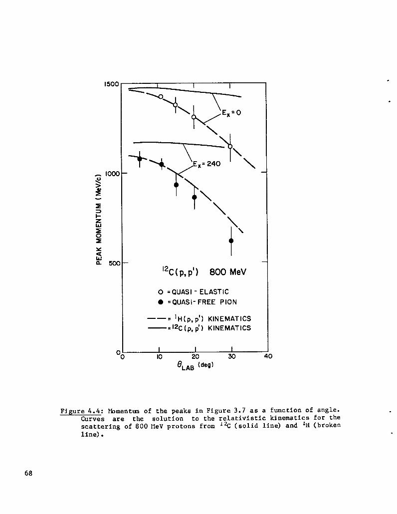
Further evidence of the dominance of
in the highly inelastic nucleon-nucleus
relation of the prominent peaks seen, namely
nucleon-nucleon processes
spectra is the kinematical
the quasi-elastic peak and
Breit-Wigner peak corresponding to a proton recoiling from a A33.
Figure 4.4 shows the momentun corresponding to the center of these
12peaks as a function of ‘lab ‘or c“ While the distortion effects
referred to above inhibit an accurate determination of the peak
locations at the larger angles, comparison of the rough locations of
these prominences with the curves corresponding to p + p kinematics and
12p+ C kinematics leads to the conclusion that the dominant processes
observed are between two nucleons.
67
‘2c(p,p’)
\
\
t
\
800 MeV
O =QUASI- ELASTIC● =QUASI-FREE PION
lH(p,p’)KINEMATICS——=
—=12C(p, p’)KINEMATICS
eLAB(degl
Figure 4.4: Ihmentun of the peaks in Figure 3.7 as a function of angle.Curves are the solution to the relativistic kinematics for thescattering of 800 MeV protons from I% (solid line) and ‘H (brokenline).
68

I
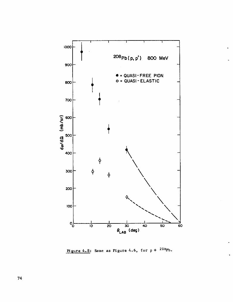
lhus the evidence is good that the cross sections for
p+ nucleus scattering to very high energy losses are dominated by,
d ‘up + nucleon processes. The — data have been divided into twodUdp
regions, corresponding to quasi-elastic scattering and quasi-free pion
production, and integrated over momentun, giving the angular
distributions
‘Ut ‘0 ‘lab =estimate of
shown in Figures 4.5-4.8. Extrapolating the% points
60° (dashed line) and integrating over angle yields an
the total cross section for nucleoxrnucleon processes in
nuclei. lhe results of this integration are given in Table 4.1, along
with the measured values for the total reaction cross section, and
Optical Model predictions for the total reaction cross section obtained
(35)using the lQITmicroscopic optical potential .
C: CONCLUSIONS:—
The information in Table 4.1 indicates that as much as 85 %
the 800 MeV p + nucleus reaction cross section may be explained
terms of nucleornucleon processes. However the conclusions to
of
in
be
drawn from the comparison of total reaction cross sections with the
d 2aangle and momentun-integrated —d~tip
are in general less obvious for the
heavier nuclei (40 208 2
Ca and12
Pb) than for H and C. First,d‘a
the —db~dp
data for the heavier nuclei do not drop off as rapidly as the lighter
nuclei at small outgoing momenta, so that the strength omitted by
cutting off the integration at - 300 MeV/c is larger. hd second, the
angular distributions that result from the momentun integration are
more sensitive to the particular extrapolation assuned for angles
69

1II+1x
IIIIIIIII
m+1
uNNh+1
1-
mdm+1
r-
Cn
N
:0.!+1
+1
.-4
r-N:
+[
+1
emmu
+1
+1
lnln
PIN
mm+1
+1
..
c.+
..

.
. 90
80
70
n~60\
:50
y 40bw
30
20
10
00
2H(p, p’) 800 MeV
● = QUAS - FREE PION
10 20 30 40 50eLAB (deg)
Figure 4.5: Angular distribution of the total pion production2H(p,p’) spectrum in Figure 3.6.contribution to the
71

.
.
+
+
12C(p, p’) 800 MeV
● =QUASI-FREE PIONO = QUASI- ELASTIC
10 20 40 50e~~~w(deg)
Figure 4.6: Fmgular distribution of the total quasi-elastic crosssection (open circles) and the total quasi-free pion production
cross section (solid dots) for p+ ‘k scattering.
.
.
)
.
.
72

.
.
00
t ‘Co (p, p’) 800 MeV
+
● =QUASI-FREE PIONo = Qu=i ‘ELASTIC
+.
10 20 30
eLAB(deg)40 50 60
Ngure 4.7: Sane as Figure 4.6, for p+ ‘°Ca.
73
moo
900
800
700
~600
>g
C!500
u%u
400
30C
200
1(X
a
1’1 I I I
~8pb( p,p’) 800 MeV
● = QUASI -FREE PION
t
o = QUASI- ELASTIC
t
(\+ \
\ \k,
\ \\\\ \ \\ \
N.N. \
1 1 I 1
10 20 30 40 50 eo
8~~8 (deg)
Figure 4.8: Same as Figure 4.6, for P + 20Mpb.
74
2 12greater than 30° in the lab. Alternately for H and C the integrated
cro.s8 section at momenta below - 300 MeV/c is small, and the angular
distributions of both the quasi-elastic and the quasi-free pion
production regions are sufficiently small at‘lab = 30° to be
relatively insensitive to the extrapolation used m larger angles.
These problems, of course, can be accommodated by measuring the
experimental cross section8 to lower outgoing momenta and larger
angles. Such an experiment is scheduled in the coming months. However
providing this data will not make the association of that cross section
with nucleon-nucleon processes more apparent.
The basis for our conclusion that only nucleon-nucleon
reactions lead to the reaction cross section is the kinematical
similarity between the p+ nucleus data and the p + p data. Based on
(36) hasthis similarity for light nuclei the Quasi-free Doorway Model
been discussed, in which the higher-multiplicityreactions are assuned
to evolve from an initial nucleoxrnucleoninteraction. Predictions of
the12C(p,p’) spectra have been published for a plan-wave calculation.
Calculations which include the distorting effects of the nuclear medium
are currently underway. ‘fhe ability of the theory to reproduce the.
data for heavier nuclei will provide a good test of the Quasi-free
Doorway Mdel.
.
7s

D: SUMMARY——
Wa have presented data for A(P,P’)X inclusive cross sections at
800 MaV, and have attempted to associate those inclusive data with .
nucleon-nucleonprocesses in nuclei. Such an association appears valid
for ligh~ nuclei, but is less obvious for heavier nuclei. Accordingly
we have found that as much as 80- 85 % of 800 MeV p + nucleus reactions
in light nuclei proceed from nucleon-nucleon interactions in the
nucleus, supporting the use of the impulse approximationfor practical
●pplications of Multiple Scattering theories. ‘lhecase for heavier
nuclei must ●wait further experimental and theoreticaldevelopments.
.
76

APPENDIX A
SYNOPSIS OF DATA FOR EXPERIMENT 470
A synopsis of the data taken in Experiment 470 is given here.
Refer to the text for a further description of the analysis.
‘lab
‘H (P,p’)so
5°Ijo
5°5°5°5°5°5°5°5°
11°11°11°11°11°11°11°ll”1111°11°~~o
11°11°15°15°15°15°15°15°15°15°15°15°
PSp
3504004806807808809801180126013201380
350400450550650750850950105011201200124012801350
340380453527601676752829898975
ntgt (nuclei/rob)
3.98x10-53.98x10-53.98x10-53.98x10-53.98x10-53.98x10-53.98X1O-53.98x10-53.98x1(J-53.98x10-53.98x10-5
3.98X1O-53.98x10-53.98x10-53.98x10-53.98x10-53.98x10-53.98x10-53.98x10-53.98 10-53.98X1O-53.98X1O-53.98x10-53.98x10-53.98x10⁻⁵
LH2LH2LH2LH 2LH2LH2LH2LH2LH2LH2
d 2Um (mb/sr/MeV/c)
.0119 t .0018
.0168 I .0024
.0324 f .0032
.0559 t .0046
.0680 * .0053
.0686 t .0060
.0985 t .0071
.0823 t .0067
.0110 t .0031
.0036 t .0030
.(IOUOt .0062
.0130 t .0U19
.0202 f .0021..0237 * .0026.0356 t .0032.0432 t .0U35.0588 * .0041.0607 t .0046.0743 ~ .0055.0747 * .0057.0674 t .0049.0280 t .0028.0022 t .0021.0000 f .0030.0180 t .0093
.0104 t .0006
.0139 k .0008
.0178 * .0011
.0262 t .0015
.0322 * .0019
.0366 t .0021
.0417 t .0025
.0473 t .0028
.0565 t .0033
.0604 t .0036
77

‘H (p,p’)
‘lab
cent’d
15°15°15015°15°15°
20020020020020020°200
25025°25°250
25025°25°250
300300300
300Cjoo
30030°3003~o
2H (p,p’)
5°5°5°5°50
5°5°50
5°5°5°5°5°
PSp
104911251150117612021229
34038048460186010101160
34038048063078093010001080
34037542655070085092510001067
35040048058068078088098010801180126013201380
%gt (nuclei/rob) = (mb/sr/MeV/c)
LH2LH 2LH2LH2LH2LH2
LH2LH2LH2LH2LH2LH2LH2
LH2LH2LH2LH2LH2LH2LH2LHz
LH2LH2LH 2LH2LH2LH2LH2LH2LH2
3.58x10-53.58X1O-53.58x10-53.58X1O-53.58x10-53.58X1O-53.58x10-53.58x10-53.58x10-53.58X1O-53.58x10-53.58x10-53.58x10⁻⁵
.0531 t .0032
.0310 * .0019
.0195 * CO012
.0045 ~ .0003
.0009 ~ .0002
.0011 * .0003
.0119 * .0015
.0141 ~ .0017
.0185 * .0010
.0219 t .0013
.0334 ~ .0022
.0237 ~ .0014
.00096 t .00005
.0114 ~ .0007
.0148 * .0010
.0170 * .0011
.0215 t .0013
.0221 ~ .0013
.0140 ~ .0009
.0057 ~ .0003
.00047 ~ .00003
.0120 ~ .0007
.0138 t .0008
.0133 t .0008
.0161 k .00U9
.0142 ~ .0008
.0072 t .0005
.0020 * .0002
.00033 ~ .0U015
.0000 f .0003
.020 f .002
.026 t .003
.043 ~ .003
.051 * .004 ‘
.070 f .005
.099 * .006
.098 k .005
.144 * .008
.154 * .009
.102 ~ .007
.031 * .004
.025 k .003
.050 * .007
.
.
.
.
78
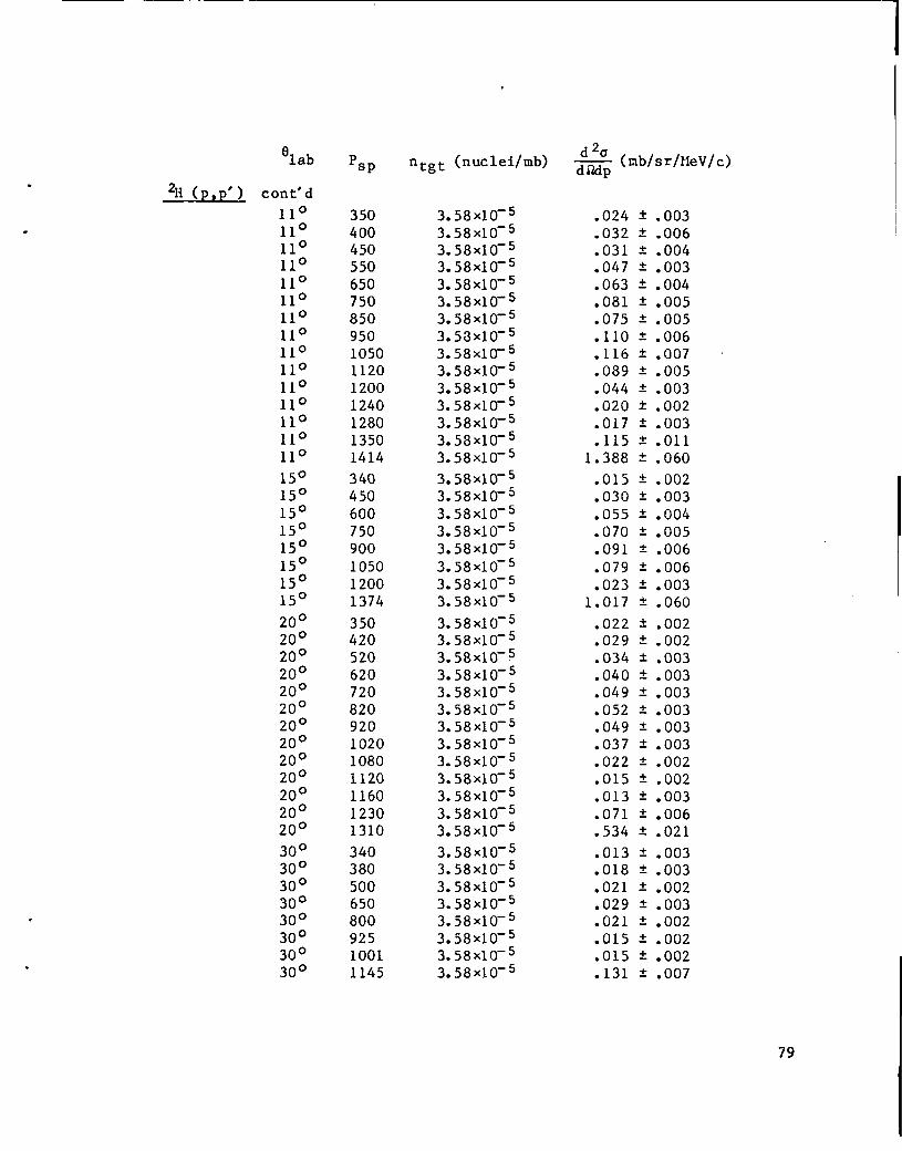
‘lab
2H (p,p’) cent’d
11°~~o
11°11011°11°11°11°110Ilo
11011011011°110
15015015°~~o
15°15°15°~50
~~o
20°20°20°.200
20°20°200
20°20°20°200
20°
30°30°30°30°30030°30°30°
PSp
3504004505506507508509501050112012001240128013501414
340450600750900105012001374
350420520620720820920102010801120116012301310
34038050065080092510011145
ntgt (nuclei/rob)
3.58x10-53.58x10-53.58x10-53.58x10-53.58x10-53.58x10-53.58x10-53.58X1O-53.58x10-53.58x10-53.58x10-53.58x10-53.58x10-53.58x10-53.58x10⁻⁵
3.58x10-53.58x10-53.58x10-53.58x10-53.58x10-53.58x10-53.58x10-53.58x10-5
3.58x10-53.58x10-53.58x10-53.58x10-53.58x10-53.58x10-53.58x10-53.58x10-53.58x10-53.58x10-53.58x10-53.58x10-53.58x10⁻⁵
3.58x10-53.58x10-53.58x10-53.58x10-53.58x10-S3.58x10-53.58x10-53.58x10-5
d 2U~ (mb/sr/MeV/c)
.024 k .003
.032 * .006
.031 f .004
.047 * .003
.063 t .004
.081 t .005
.075 t .005
.110 t .006
.116 k .007
.089 t .005
.044 ~ .003
.020 * .002
.017 * .003
.115 ~ .0111.388 * .060
.015 * .002
.030 ~ .003
.055 * .004
.070 ~ .005
.091 * .006
.079 t .006
.023 I .0031.017 * .060
.022 f .002
.029 * .002
.034 ~ .003
.040 * .003
.049 ~ .003
.052 t .003
.049 * .003
.037 ~ .003
.022 * .002
.015 f .002
.013 ~ .003
.071 t .006
.534 ~ .021
.013 f .003
.018 * .003
.021 ~ .002
.029 t .003
.021 ~ .002
.015 ~ .002
.015 f .002
.131 ~ .007
79

Olab Psp ntgt (nuclei/rob)
‘% (p,p’)
5° 350 8.73x10-650 400 8.73x10-65° 480 8.73x10-65° 580 8.73x10-65° 680 8.73x10-65° 780 8.73x10-65° 880 8.73x10⁻⁶so 980 8.73x10-65° 1080 8.73x10-650 1180 8.73x10-65° 1260 8.73x10-650 1320 8.73x10-650 1380 8.73x10⁻⁶
11° 350 8.73x10-611° 400 8.73x10⁻⁶~~o 450 8.73x10-611° 550 8.73x10⁻⁶~~o 650 8.73x10⁻⁶~~o 750 8.73x10-611° 850 8.73x10-611° 950 8.73x10-611° 1050 8.73x10-611° 1120 8.73x10-611° 1200 8.73x10-611° 1240 8.73x10-611° 1280 8.73x10-611° 1350 8.73x10⁻⁶~lo 1414 8.73x10⁻⁶
15° 340 2.30x10⁻⁶ ‘15° 450 2.30x10-615° 600 2.30x10⁻⁶~50 750 2.30x10-615° 900 2.30x10-615° 1050 2.30x10-615° 1200 2.30x10-615° 1374 2.30x10⁻⁶
20° 350 8.73x10-6200 420 8.73x10-620° 520 8.73x10-620° 620 8.73x10-6200 720 8.73x10-620° 820 8.73x10-602~o 920 8.73x10⁻⁶zoo 1020 8.73x10-620° 1080 8.73x10⁻⁶
d 2a~ (mb/sr/MeV/c)
.079 * .004
.108 * .005
.131 * .006
.173 t .008
.212 * .009
.241 i .010
.275 * .011
.329 * .014
.408 t .017
.348 t .014
.184 t .008
.175 * .008
.392 * .016
.101 * .004
.108 t .005
.133 f .006
.156 t .006
.182 * .007
.204 t .008
.231 t .009
.240 * .010
.263 t .011
.227 t .009
.152 t .006
.137 t .006
.158 t .007
.618 * .0251.709 * .063
.084 * .006
.115 t .006
.157 * .008
.186 ~ .010
.204 * .011
.196 t .010
.150 t .008
.980 t .048
.098 * .005
.115 t .006
.129 f .006
.141 * .007
.146 k .007
.149 f .007
.149 ~ .007
.134 * .007
.124 i .006
.
.
.
.
80

.
‘lab
1% (p,p‘) cent’d.~~o
20°200
30°30°30°30°30°30°30°30°
40Ca (p,p’)
5°5°5°5°5°5°5°5°5°5°5°5°50
11°11°11°11°11°11°11°11°11°11°11°11°11°11°11°
15°15°15°15°
PSp
1120116012301310
34038050065080092510001145
35040048158068078088098010801180126013201380
3504004505506507508509501050112012001240128013501414
340450600750
ntgt (nuclei/mb) ~ (mb/sr/MeV/c)
8.73x10-68.73x10-68.73x10-68.73x10-6
2.30x10-62.30x10-62.30x10-62.30x10-62.30x10-62.30x10-62.30x10-62.30x10-6
2.19x10-62.19x10-62.19x10-62.19x10-62.19x10-62.19x10-62.19x10-b2.19x10-62.19x10-62.19x10-62.19x10-62.19x10-62.19x10⁻⁶
2.19x10-62.19x10-62.19x10-62.19x10-62.19x10-62.19x10-62.19x10-62.19x10-62.19x10-62.19x10-62.19x10-62.19x10-62.19x10-62.19x10-62.19x10⁻⁶
7.29x10-77.29x10-77.29x10-77.29x10-7
. 133 f .007
.169 t .008
.316 * .016
.449 * .021
.077 * .005
.088 * .006
.103 * .005
.108 t .006
.099 * .005
.099 ~ .005
.116 * .006
.149 ~ .008
.262 ~ .012
.310 ~ .015
.356 * .016
.389 t .019
.426 t .021
.505 * .023
.495 ~ .023
.575 t .026
.704 ~ ●030
.644 * .028
.357 * .016
.306 t .015
.841 f .038
.334 f .014
.332 * .014
.377 t .016
.389 t .017
.403 ~ .017
.431 t .018
.443 ~ .019
.466 i .020
.476 t .020
.413 ~ .018
.311 ~ .013
.268 * .012
.277 t .0121.024 * .0442.80 ~ .11
.268 I .020
.330 * .018
.405 f .021
.405 ~ .022
81
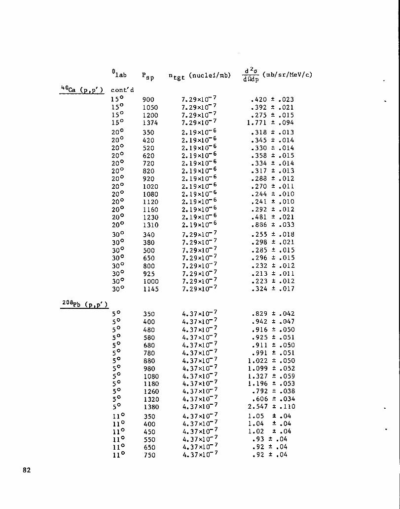
..
‘lab P~p
40Ca (p,p‘) cent’d
15°15°~50
15°
20°200
20°20°20°20°20°20020°20°20°20°20°
30030°30°30°30°30°30°30°
208pb ( ●)
50505050so
5°5050
5°5°5°5050
11°11°11°
900105012001374
350420520620720820920102010801120116012301310
34038050065080092510001145
35040048058068078088098010801180126013201380
350400450550650750
ntgt (nuclei/rob)
7.29x10-77.29x10-77.29x10-77.29x10-7
2.19x10-62.19x10-62.19x10-62.19x10-62.19x10-62.19x10-62.19x10-62.19x10-62.19x10-62.19x10-62.19x10-62.19x10-62.19x10⁻⁶
7.29x10-77.29x10-77.29x10-77.29x10-77.29x10-77.29x10-77.29x10-77.29x10-7
4.37X1O-74.37X1O-74.37X1O-74.37X1O-74.37X1O-74.37X1O-74037X10-74.37X1O-74.37X1O-74.37X1O-74.37X1O-74.37X1O-74.37X1O-7
4.37X1O-74.37X1O-74.37X1O-74.37X1O-74.37X1O-74.37X1O-7
% (mb/sr/MeV/c)
.420 * .023
.392 t .021
.275 * .0151.771 * .094
.318 t .013
.345 f .014
.330 * .014
.358 t .015
.334 ~ .014
.317 f .013
.288 t .012
.270 t .011
.244 t .010
.241 * .010
.292 * .012
.481 t .021
.886 ~ .033
.255 * .018
.298 t .021
.235 t .015
.296 t .015
.232 t .012
.213 t .011
.223 * .012
.324 * .017
.829 * .042
.942 t .047
.916 i .050
.925 t .051
.911 ~ .050
.991 * .0511.022 ~ .0501.099 t .0521.327 t .0591.196 * .053.792 * .038.606 ~ .034
2.547 * .110
1.05 * .041.04 * .041.02 ~ .04.93 ~ .04.92 ~ .04.92 t .04
.
.
.
82
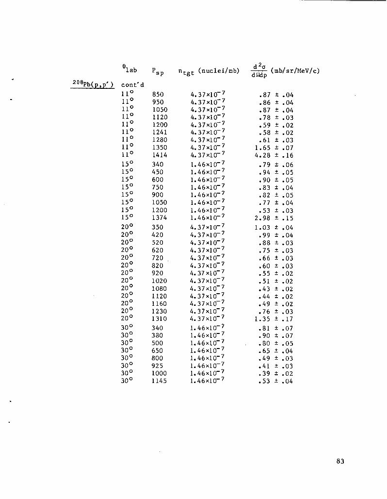
‘lab P~p
208pb(9P‘) cent’d
11°11°11°11°11°~~o
11°~~o
11°
15°15°15°15°15°15°~50
150
20020°20°20°20°20°20°20°20020°20°.200
20°
30°30°30°30°30°30°30°30°
8509501050112012001241128013501414
340450600750900105012001374
350420520620720820920102010801120116012301310
34038050065080092510001145
ntgt (nuclei/rob)
4.37X1O-74.37X1O-74.37X1O-74.37X1O-74.37X1O-74.37X1O-74.37X1O-74.37X1O-74.37X1O-7
1.46x10-71.46x10-71.46x10-71.46x10-71.46x10-71.46x10-71.46x10-71.46x10-7
4.37X1O-74.37X1O-74.37X1O-74.37X1O-74.37X1O-74037X10-74.37X1O-74.37X1O-74.37XI0-74.37X1O-74.37X1O-74.37X1O-74.37X1O-7
1.46x10-71.46x10-71.46x10-71.46x10-71.46x10-71.46x10-71.46x10-71.46x10-7
d 2am (mb/sr/MeV/c)
83

APPENDIX B
A FAST, LOWMASS DETECTOR FOR CHARGED PARTICLES
by J. A. McGill, L. G. Atencio, and C. L. Morris
Nuclear Instruments and Methods (to be published)
.
.
Multi-wire proportional counters (MWPC) using delay lines
and one amplifier per wire have been described in the literature .
A good review of such counters is given in Reference 39, and
references therein. In this paper we describe a MWPC designed to
operate at significantly reduced gas pressures, and to provide
positjon, time, and angle information. It presents a low mass to
charged particlea traversing it, and is intended to be used with a
small beam. The specific detector descrjbed was built as an
upstream profile monitor for an 800 WV proton beam.
CONSTRUCTION and INSTALLATION
The body of the counter was machined from a 4“ x 2~’ x 2“
aluminum block as shown in Figure B1. A piece of 2(I w # Au-pldted
tungsten wire (a) was strung down the center of each of the three
1bores,
z“soldered at one end to a modified S1lVconnector (b).
Prior to this each S}{Vconnector had its solder tip cut back, and a
0.6mm hole was drilled therein at the geometric center of the
threads. With the connector and wire installed, the other end of
84

fQ
Fjgure Bl: An assembly drawing of the chamber described, showingthe position of an anode wire (a), SHV connectors (b), one ofthree lucjte centering plugs (c), one of the 0.(IU05° mylarwindows. &s from tilehandling system entered t}lroughone of
the ~’ poly-flo lines (e) and exitted the other, witl~
cros-flow provided by the $’ holes (f).
85

.
.
* 2’”0+
\
0.0005-in. MYLAR \BRAssPLATE
Figure B2: Detail of the interface between the chamber Imly,~ Inj1mylar window, and the brass plate.
.
.
86

the wire was threaded through a lucite centering plug (c), a 30 gm.
tensioning weight was attached, and the wire and plug were secured
with epoxy.
The oblong hole through the 2;’ dimension of the block was
covered at each end with a .0005” Mylar window (d) sandwiched
between a brass plate and the block. All edges were rounded and
smeared with a light film of silicon grease to keep the epoxy at
the perimeter of the Mylar, allowing the Mylar to flex without
encountering any sharp edges (Figure S2).
Poly-flo fittings (Figure Bl(e)) provided gas eIILryaLld
exit, with cross-flow between wires through ~’ holes (f). These
holes were plugged to the environment with epoxy. The gas handling
system is shown in Figure B3. Gas pressure in the chamber is
monitored by a 0-800 mm differential pressure gauge installed as
shown. The ilanostatused to regulate gas pressure was advertised
as capable of maintaining a constant pressure over a wide range of
thru-rates, but in reality some adjusting was necessary to achieve
a specific combination of flow and pressure. However once set, tile
N!anostat was quite stable over periods of up to 72 hrs.
87

1-
d
@
(.O=
a_w
Iu
5(1-U?0zaz
..
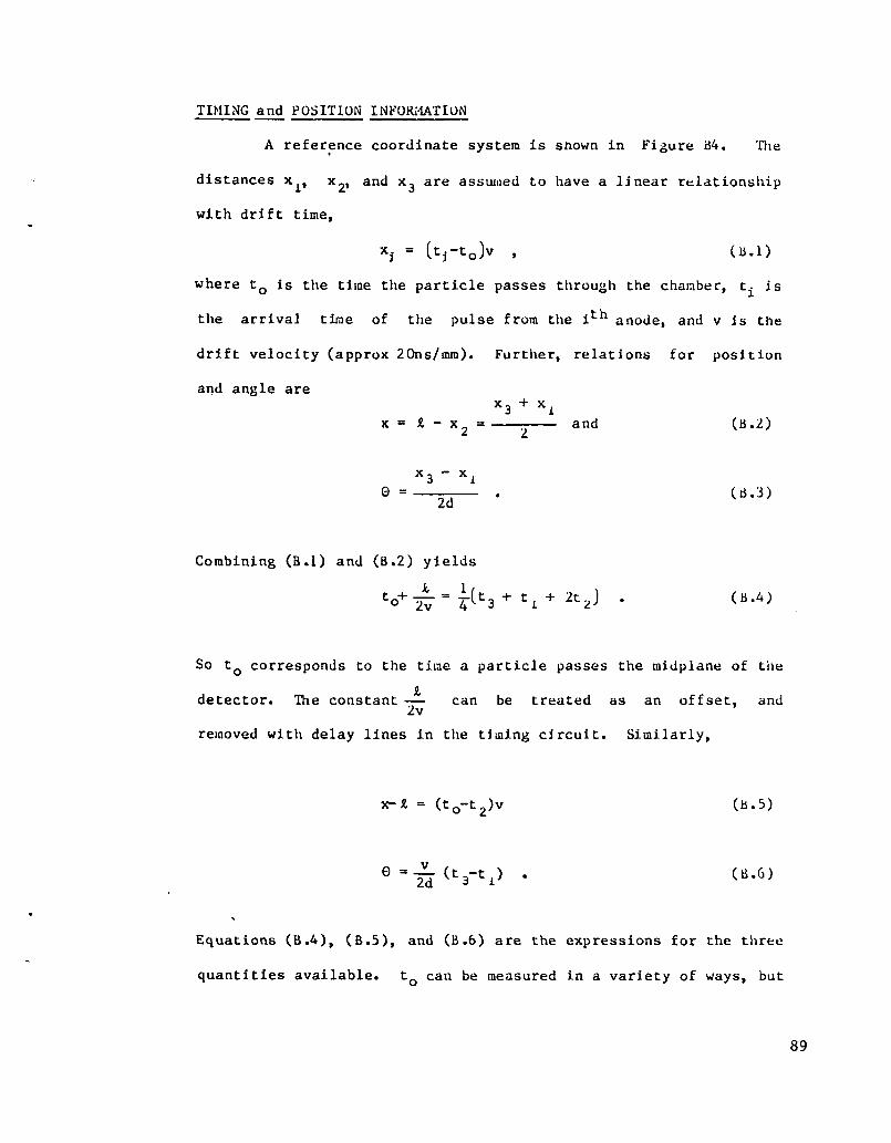
.
.
TIMING and POSITION 1NFUUATION—.
A reference coordinate system is shown in Figure U4. The
distances XL, X2, and X3 are assumed to have a linear relationship
with drift time,
x. =J (tj-to)v , (B.1)
where to is the time the particle passes through the chanber, ti is
the arrival time of the pulse from the ith anode, and v is the
drift velocity (approx 20ns/min). Further, relations for position
and angle are
‘3 + ‘1x= 2-X2=
2and
‘3 - ‘10=
2d “
Combining (B.1) and (B.2) yields
t~+k
K=#t3+t, +2t2) . (B.4)
SO to corresponds to the time a particle passes the midplane of the
detector. ‘l%econstant +
removed with delay lines in
(B*2)
(t3.3)
can be treated as an offset, and
the timing circuit. Similarly,
x-t= (to-t2)v
e =;(t3-t J .
(B.5)
(B.6)
.
Equations (B.4), (B.5), and (B.6) are the expressions for the three
quantities available. to can be measured in a variety of ways, but
89
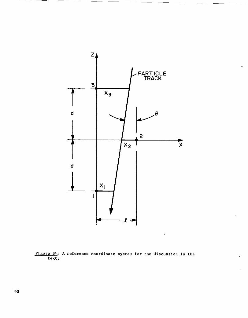
d
d
L
x3
X2 x
Xj
.
Figure B4: A reference coordinate system for the discussion in thetext.
.

.
.
*
.
the most straitforward is to
Corp. model # 624, to obtain
t.
use a meantiuier, ego Lecroy &search
+t.tt
12=~
2
Then
to = ~j(t2t3)+ offset .
The time differences can be calculated using TAC’S or TUC’S, and
added together either with summing amplifiers or in software to
obtain the other quantities.
RES’ULTS
Some plateau curves as a function of pressure are shown in
Figure B5. For minimum ionizing particles, the device appears to
be useful at pressures above 180 ma1ig abs. Below these pressures
anode efficiencies are less than til)%,and the plateau shoulder is
too narrow to trust. At 300 mm~{gthe counter is N 7 nlg/ca2 thick,
including the ~ mil Mylar .windowso The drift spectra in Figure Bb
were taken with a 207Bj source collimated to - 6mm. The drift
velocities do not change measurably over a wide range of pressures,
but stay constant at 20ns/mm.
In several trials with an 800 MeV proton beal~ raw signals
from the chamber had - 5rnvamplitudes with 2ns rise times, when
terminated into 50 $2. By plac~.nga scintillator directly behind
the counter, the tjme resolution between the scintjllator and to
was measured to be 2 ns FWHM. The ultimate position resolution is
expected to be *.1 mm based on previous drift chamber
91

EE0C9
2
1,,1,,
I1
I1,1,,,
11
1—
0
(%)
A9N
3131=J=
J3
un002
~a-0
-$3
●
92

..
--
-T-
I
3a
131A
●u
,
93

(39)measurements . Based on the position resolution one should be
able to obtain an angle resolution of -4 mrad with the present
counter,
The countinb~rate performance of
space charge effects, and consequently
size. Problems are expected to arise at
104/ l~near mm of wire/ sec.
the counter is limited by
depends upon the beam spot
counting rates exceeding
CONCLUSION
We have reported a small counter which presents a mass of
7 mg/cm2 to incident particles and is capable of providing time,
position, and angle information. I.njtialstudies have shown it is
possible to obtain better than 2 ns FWIL1time resolution. Expected
position resolutions are ().1mm and expected angle resolutions are
4 mrad.
94

.
.
Appendix C
Listed below is the Test Descriptor file used in
Experiment 470.
601,65,5S,4,Box 1,Box 2,Box 3,IOR.-I. I.END iGATEC?.TECATECATEGATEGATE
1,1,-1,1.1,-1,1,1,-1,1,1 !-1,12,20,600,13.20.600.
BI ,2,6,”BI ,2,7,CA,14109871,10155,CA,142,99OO,1OIOO,CA, I43,99OO,1OIOO,CA,144,9900, IO1OO,CA,145,9900, 1O1C)O,CA,146, %B7,10169,BOX 4,CA,239,998O,1OO2O,r3A,~40, 9980, loo~o ,CA.185.8500,11500,CA,181 ,13000,7000,ICAT 1,ICAT 2,lCAT 3,ICAT 4,lC?.TS,CA,160,7500, 1250t3,CA,148,9800,10200,CA,162,7SO0,12500,CA, I5O,98OO,1O2OO,BOX,5,BOX,6,BOX,7,BOX.8.BOX,9,CA,193, 1OO2O,1OO6O,CA, 193,9985, 10045,CA,193, 10045,10105,CA, 193,I0105. IO165,CA,193,9B72,1014S,CA. 193,9890,10239.CA,181; 13000,7000:CA,181,13QQ0,7000,AND, -5,-6,AND, -7,-8,AND,46,47,AND, I,l,AND,20,21,AND, 13,18,AND, 14,15,16,17,AND, 14,15,16,17,49AND, 14,15,16,17,49AND,20,33,49,52,AND,21 ,33,49,52,AND,20,53,AND,21 ,53,AND,54,19,AND,2,19,50, !J2,AND, 15,16,17,49,21AND, 14,16,17,49,21AND, 14,15,17,49,20AND, 14,15,16,49,20AND,3,19,50, S2,.
.
,33,,50,
,33.,33,,33.,33,
:[16!J,761BIW470. TST CYCIJ5.2iJ DEC 1979:1 INSIDE BOX -- 1 . PID:2 2:3:4 LOOP 1 coum3
I5 SPARE16 SP.ARE:7 SPARE:8 SPARE;9 NORM:10111;12113114:1s;16;17118;19120;21:22I23I24:23:26:27:28;29:30;31;32833:34;35$36;37;38I39140;41:42;43:44;45:46:47t48149850;51152
:34
:57;58I59169161162163;64165
SPARESPARECNMBR 1 CEKSUN
234
:ANCLE CUT==> X(-185) VS ROTATED ARCLS (.196)DRF DIFF 23 (+/- 2MM)DRF DIFF 45 (+/- 2NM)X DRIFT CBMMERSSP.AREPEAK
;345
CR2XCHZYCH4XCH4YBOX 5BOX 6BOX 7BOX 8BOX 9SCAT7 ANCLE 1
. 2
. 2
,FULL S~ ANC!E RXCION 2 DECREESsPlmESPARENOT JAWSNOT VETOESNOT ANTISGOOD PID ==> NO ANTIS, PillDRY TSTDL OKDR OK
:53 DR CBMBRS, GOOD PID,BOX5DR CHMBRS , GOOD P !D , DRP TST
;55 DR CBRS, COOD PID,DRF23, BOX5$56 DR CHBNS, COOD PID,DlW43, B0X5
TEST 53 AND DRF23TEST 53 AND DRF45GOOD EVENT ==> GOOD PID, DR CBS, XANCLE, DRFGOOD BOX 2 EVENTALL DR CRMBRS BUT 2, GOOD PID, DRF45,BOXS
34 DRP235
GOOD BOX 3 EWNT
95

,
.
AND,59,42,AND,59.34.3B$AND. s9,40mAND;S9,41,AND, S9,42,AND, S9,24,AND, S9,24,34,AND,S9,26,AND, S9,27,AlfD,S9,28,AND,22.42,59,AND,35,S9,AND,22,42,60,AND.22,42,6S,AND,22, S9,AND, -16,17,49,AND, S9,33.AND,69,34,AND,69,3S,AND.69,36,AND 59,36,AND,S9,39,AND, s9,4eoARD, S9,41,AND. S9,42,AND.3,19.22,42 .Se,s2,IOR,l,-l,ENDFINISH
g66 COOD167 GOOD168:69
EVENT , SCAT ANCLE SEVENT SCAT REG 1 VAW
4;70 s;71 COOD EVENT, PEAK 1;72 GOOD EVENT PEAX 13=A TCI’;73:74 4175;76 X DRI?T CSAI’IBERS&)OD EVENT SCAT REGION 5177 BOX 7 AND GOOD EVENT;78 X DRIFT CBAMBERS, GOOD EVW Box 2! scAmlNc .mcu179 x DRIFT CBAI’IB~. cooD EVENT Box 30 s~T ~cXOH s;80 COOD EVENT, X DRIFT .~-;81 DRIFT S, NOT 4, ~oD PID;82 GOOD EVENT, BOX s:83 6.——104 7:85186 000D EVENT 80X 88;87 COOD EVENT, SCAT ANCLE 2180 3;89 4.—-;90
191 PID12 EQUIVALE% OF TES1’ 76;92 LOOP 2 COUNTER
REGION 5
.
.
96

ACKNOWLEDGME~
b.
As is usually the case, those who have gone before have nade
straight the way for those who follow. In particular I am grateful to
the LMPF staff and users who have contributed to the hardware and
software which facilitated the experiments described here. Special
thanks go to Jim Amann for his fervent efforts. The collaborators on
these experiments also rendered specific assistance, most notably Ray
Fergerson, Cas Milner, and George Burleson. Martin Barlett not only’
collaborated in the collection of the data, but also in many hours of
discussions and “thinking out loud.” Of course Gerry Hoffmann, my
thesis advisor, deserves my greatest appreciation for the help and/
guidance he has given throughout the last three years.
This work was supported by the Department of Energy and by The
Robert A. Welch Foundation.
“
.
97
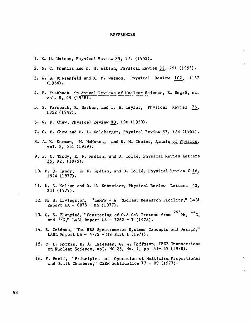
REFERENCES
1. K. M. Watson, Physical Review~, 575 (1953).
2. N. C. FYancis and K. M. Watson, Physical Review 9&, 291 (1953).
3. W. B. Riesenfeld and K. M. Watson, Physical Review ~, 1157(1956).
4. H. Feshbach in Annual Reviews of Nuclear Science, E. Segr&, ed.vol. 8, 49 (1958).
—
5. S. Fernbach, R. Serber, and T. B. ‘Ikylor, Physical Review ~,1352 (1949).
6. G. F. Chew, Physical Review 80, 196 (1950).
7. G. F. Chew and M. L. Goldberger, Physical Review~, 778 (1952).
8. A. K. Kerman, M. Iklfanus, and R. M. Thaler, lmnals of Physics,—VO1. 8, 551 (1959).
9. P. C. Tandy, E. F. Redish, and D. B0116, Physical Review Letters
10.
11.
12.
13.
14.
15.
16.
35, 921 (i975).
P. C. Tandy, E. F. Redish, and D. E0116, Physical Review CM,1924 (1977).
D. S. Koltun and D. M. Schneider, Physical Review Letters ~,211 (1979).
M. S. Livingston, “LAMPF - A Nuclear Research Facility,” LASLReport LA- 6878 -MS (1977).
G. S. Blanpied,208 12
“Scattering of 0.8 GeV Protons from Pb, C,and ‘3C,” LASL Report LA- 7262 - T (1978).
B. Zeidnan, “The HRS Spectrometer System: tincepts and Design,”LASL Report LA- 4773 -MS Part I (1971).
C. L. Ibrris, H. A. ‘lhiessen,G. W. Hoffmann, IEEE Transactionson Nuclear Science, vol. NS-25, No. 1, pp 141-143 (1978).
F. Sauli, “Principles of Operation of Multiwire Proportionaland Drift Chambers,” CERN l%blication 77 - 09 (1977).
98

17.
1.8.
19.
20.
21.
22.
23.
24.
25.
26.
27.
28.
29.
30.
31.
32.
33.
34.
35.
36.
“A Modular Instrumentation System for Data Handling, ” EuratomReport EUR - 4100e (1969).
B. Zacharov, “CAMAC Systems: A Pedestrian’s Guide,” DaresburyNuclear Physics Laboratory, Daresbury, lhgland (1972).
M. Kellogg, 110M. Minor, S. Schlaer, N. Spencer, R. F.Thomas Jr., and H. van der Beken, “Introduction to Q“, LASLReport LA- 7001 -M (1978).
M. Kellogg et al., “QAL and the Analyzer——LA- 6884 -M (1977).
R. J. Ridge, “DSP - A Histogram Display(1979).
A. Wriekat et al., Physics Letters, to be.—
Task”, LASL Report
Program”, unpublished
published.
G. W. Hoffmann et al., Physical Review C~, 1488 (1980).——
R. E. Chrien et al., Physical Review C~, 1014 (1980).——
L. Ray et al., Physical Review C=, 828 (1980).——
L. Ray, University of Texas, Austin, Texas, unpublished.
G. S. klams et al., Physical Review C~, 2485 (1980).——
P. V. Vavilov, JETP (USSR) ~, 749 (1957).
H. A. Bethe, Physical Review~, 1256 (1953).
W. T. Scott, Reviews of lbdern Physics=, 231 (1963).
P. R. Bevington, Data Reduction and Error Analysis for thePhysical Sciences, lkGraw - Hill~.Y. (1969). —
J. Hudomalj - Gabitzsch et al., Physical Review CM, 2666(1978).
——
E. Ferrari and F. Selleri, Nuovo Cimento~, 1028, (1961).
&Ynter Wolf, Physical Review 182, 1538 (1966).
L. Ray, Physical Review C~, 1857 (1979).
Y. Alexander, J. W. van Orden, E. F. Redish, and S. J. Wallace,Physical Review Letters @ 1579 (1980).
99

Dometiic NTISPage Range Price Price Code
001425 s .5.00 A02026.050 6.OO A03051.075 7.00 A04076-100 8.04 A05101-12s 9.00 A06126-150 10.00 A07
Printed in the United States of AmericaAvailable from
National Technical Information ServiceUS Department of Commerce
S285 Port Royal RoadSpringIicld, VA 22161
Microfiche S3.50 (AOI)
Domestic NTIS Domestic NTlsPage Range Rice Price Code Page Range RiLX Price Code
1s1-175 $11.00 AOg 301-325 S17.00 A14176-200 12.00 A09 326-35o 18.00 AM201-225 13.00 AlO 3s1-375 19.00 A16
226-250 14.00 All 376400 20.00 A17
2S1-27S 15.00 A12 401425 21.00 A18
276-300 16.00 A13 4264s0 22.00 A19
Domestic NTISPage Range Rice Price Code
451475 S23.00 A20476-500 24.00 A21
501-525 25.00 A22S26-S50 26.oo A235s1-575 27.00 A24
576.600 28.00 A25601-uP t AW
tAdd S1.00 for each addltioml 25.page increment or portion thereof from 601 pages up.


![1 Pensions (FAS 87); Post Retirement Benefits (FAS 106); Post Employment Benefits (FAS 112); Disclosure about Pensions, etc. (FAS 132 [R]) – amendment](https://img.dokumen.tips/doc/110x75/56649d1f5503460f949f3b1c/1-pensions-fas-87-post-retirement-benefits-fas-106-post-employment-benefits.jpg)