Representation and Querying of Valid Time ofTriples in Linked Geospatial Data ?

Konstantina Bereta, Panayiotis Smeros, and Manolis Koubarakis

National and Kapodistrian University of Athens, Greece{Konstantina.Bereta, psmeros, koubarak}@di.uoa.gr

Abstract. We introduce the temporal component of the stRDF datamodel and the stSPARQL query language, which have been recently pro-posed for the representation and querying of linked geospatial data thatchanges over time. With this temporal component in place, stSPARQLbecomes a very expressive query language for linked geospatial data, go-ing beyond the recent OGC standard GeoSPARQL, which has no supportfor valid time of triples. We present the implementation of the stSPARQLtemporal component in the system Strabon, and study its performanceexperimentally. Strabon is shown to outperform all the systems it hasbeen compared with.

1 Introduction

The introduction of time in data models and query languages has been thesubject of extensive research in the field of relational databases [6, 20]. Threedistinct kinds of time were introduced and studied: user-defined time which hasno special semantics (e.g., January 1st, 1963 when John has his birthday), validtime which is the time an event takes place or a fact is true in the applicationdomain (e.g., the time 2000-2012 when John is a professor) and transaction timewhich is the time when a fact is current in the database (e.g., the system timethat gives the exact period when the tuple representing that John is a professorfrom 2000 to 2012 is current in the database). In these research efforts, manytemporal extensions to SQL92 were proposed, leading to the query languageTSQL2, the most influential query language for temporal relational databasesproposed at that time [20].

However, although the research output of the area of temporal relationaldatabases has been impressive, TSQL2 did not make it into the SQL standardand the commercial adoption of temporal database research was very slow. It isonly recently that commercial relational database systems started offering SQLextensions for temporal data, such as IBM DB2, Oracle Workspace manager, andTeradata [2]. Also, in the latest standard of SQL (SQL:2011), an important newfeature is the support for valid time (called application time) and transactiontime. Each SQL:2011 table is allowed to have at most two periods (one for

?This work was supported in part by the European Commission project TELEIOS(http://www.earthobservatory.eu/)

application time and one for transaction time). A period for a table T is definedby associating a user-defined name e.g., EMPLOYMENT TIME (in the case ofapplication time) or the built-in name SYSTEM TIME (in the case of transactiontime) with two columns of T that are the start and end times of the period(a closed-open convention for periods is followed). These columns must havethe same datatype, which must be either DATE or a timestamp type (i.e., nonew period datatype is introduced by the standard). Finally, the various SQLstatements are enhanced in minimal ways to capture the new temporal features.

Compared to the relational database case, little research has been done toextend the RDF data model and the query language SPARQL with temporalfeatures. Gutierrez et al. [8, 9] were the first to propose a formal extension of theRDF data model with valid time support. They also introduce the concept ofanonymous timestamps in general temporal RDF graphs, i.e., graphs containingquads of the form (s, p, o)[t] where t is a timestamp or an anonymous timestamp xstating that the triple (s, p, o) is valid in some unknown time point x. The workdescribed in [11] subsequently extends the concept of general temporal RDFgraphs of [9] to express temporal constraints involving anonymous timestamps.In the same direction, Lopes et al. integrated valid time support in the generalframework that they have proposed in [15] for annotating RDF triples. Similarly,Tappolet and Bernstein [22] have proposed the language τ -SPARQL for queryingthe valid time of triples, showed how to transform τ -SPARQL into standardSPARQL (using named graphs), and briefly discussed an index that can be usedfor query evaluation. Finally, Perry [19] proposed an extension of SPARQL,called SPARQL-ST, for representing and querying spatiotemporal data. Themain idea of [19] is to incorporate geospatial information to the temporal RDFgraph model of [9]. The query language SPARQL-ST adds two new types ofvariables, namely spatial and temporal ones, to the standard SPARQL variables.Temporal variables (denoted by a # prefix) are mapped to time intervals andcan appear in the fourth position of a quad as described in [9]. In SPARQL-STtwo special filters are introduced: SPATIAL FILTER and TEMPORAL FILTER. Theyare used to filter the query results with spatial and temporal constraints (OGCSimple Feature Access topological relations and distance for the spatial part,and Allen’s interval relations [3] for the temporal part).

Following the ideas of Perry [19], our group proposed a formal extension ofRDF, called stRDF, and the corresponding query language stSPARQL for therepresentation and querying of temporal and spatial data using linear constraints[13]. stRDF and stSPARQL were later redefined in [14] so that geometries arerepresented using the Open Geospatial Consortium standards Well-Known-Text(WKT) and Geography Markup Language (GML). Both papers [13] and [14]mention very briefly the temporal dimension of stRDF and do not go into de-tails. Similarly, the version of the system Strabon presented in [14], which im-plements stRDF and stSPARQL, does not implement the temporal dimension ofthis data model and query language. In this paper we remedy this situation byintroducing all the details of the temporal dimension of stRDF and stSPARQLand implementing it in Strabon.

The original contributions of this paper are the following. We present indetail, for the first time, the valid time dimension of the data model stRDF andthe query language stSPARQL. Although the valid time dimension of stRDF andstSPARQL is in the spirit of [19], it is introduced in a language with a much moremature geospatial component based on OGC standards [14]. In addition, thevalid time component of stSPARQL offers a richer set of functions for queryingvalid times than the ones in [19]. With the temporal dimension presented in thispaper, stSPARQL also becomes more expressive than the recent OGC standardGeoSPARQL [1]. While stSPARQL can represent and query geospatial data thatchanges over time, GeoSPARQL only supports static geospatial data.

We discuss our implementation of the valid time component of stRDF andstSPARQL in Strabon. We evaluate the performance of our implementation ontwo large real-world datasets and compare it to three other implementations: (i)a naive implementation based on the native store of Sesame which we extendedwith valid time support, (ii) AllegroGraph, which, although it does not offer sup-port for valid time of triples explicitly, it allows the definition of time instantsand intervals and their location on a time line together with a rich set of func-tions for writing user queries, and (iii) the Prolog-based implementation of thequery language AnQL1, which is the only available implementation with explicitsupport for valid time of triples. Our results show that Strabon outperforms allother implementations.

This paper is structured as follows. In Section 2 we introduce the temporaldimension of the data model stRDF and in Section 3 we present the temporalfeatures of the query language stSPARQL. In Section 4 we describe how we ex-tended the system Strabon with valid time support. In Section 5 we evaluate ourimplementation experimentally and compare it with other related implementa-tions. In Section 6 we present related work in this field. Section 7 concludes thispaper.

2 Valid Time Representation in the Data Model stRDF

In this section we describe the valid time dimension of the data model stRDFpresented in [14]. The time line assumed is the (discrete) value space of thedatatype xsd:dateTime of XML-Schema. Two kinds of time primitives are sup-ported: time instants and time periods. A time instant is an element of the timeline. A time period (or simply period) is an expression of the form [B,E), (B,E],(B,E), or [B,E] where B and E are time instants called the beginning and theending of the period respectively. Since the time line is discrete, we often as-sume only periods of the form [B,E) with no loss of generality. Syntactically,time periods are represented by literals of the new datatype strdf:period thatwe introduce in stRDF. The value space of strdf:period is the set of all timeperiods covered by the above definition. The lexical space of strdf:period istrivially defined from the lexical space of xsd:dateTime and the closed/open pe-

1http://anql.deri.org/

riod notation introduced above. Time instants can also be represented as closedperiods with the same beginning and ending time.

Values of the datatype strdf:period can be used as objects of a triple torepresent user-defined time. In addition, they can be used to represent validtimes of temporal triples which are defined as follows. A temporal triple (quad)is an expression of the form s p o t. where s p o. is an RDF triple and t is atime instant or a time period called the valid time of a triple. An stRDF graphis a set of triples and temporal triples. In other words, some triples in an stRDFgraph might not be associated with a valid time.

We also assume the existence of temporal constants NOW and UC inspiredfrom the literature of temporal databases [5]. NOW represents the current timeand can appear in the beginning or the ending point of a period. It will be usedin stSPARQL queries to be introduced in Section 3. UC means “Until Changed”and is used for introducing valid times of a triple that persist until they areexplicitly terminated by an update. For example, when John becomes an asso-ciate professor in 1/1/2013 this is assumed to hold in the future until an updateterminates this fact (e.g., when John is promoted to professor).

Example 1. The following stRDF graph consists of temporal triples that repre-sent the land cover of an area in Spain for the time periods [2000, 2006) and[2006, UC) and triples which encode other information about this area, suchas its code and the WKT serialization of its geometry extent. In this and fol-lowing examples, namespaces are omitted for brevity. The prefix strdf standsfor http://strdf.di.uoa.gr/ontology where one can find all the relevantdatatype definitions underlying the model stRDF.

corine:Area_4 rdf:type corine:Area .corine:Area_4 corine:hasID "EU-101324" .corine:Area_4 corine:hasLandCover corine:coniferousForest

"[2000-01-01T00:00:00,2006-01-01T00:00:00)"^^strdf:period .corine:Area_4 corine:hasLandCover corine:naturalGrassland

"[2006-01-01T00:00:00,UC)"^^strdf:period .corine:Area_4 corine:hasGeometry "POLYGON((-0.66 42.34, ...))"^^strdf:WKT .

The stRDF graph provided above is written using the N-Quads format2 whichhas been proposed for the general case of adding context to a triple. The graphhas been extracted from a publicly available dataset provided by the EuropeanEnvironmental Agency (EEA) that contains the changes in the CORINE LandCover dataset for the time period [2000, UC) for various European areas. Ac-cording to this dataset, the area corine:Area_4 has been a coniferous forestarea until 2006, when the newer version of CORINE showed it to be naturalgrassland. Until the CORINE Land cover dataset is updated, UC is used to de-note the persistence of land cover values of 2006 into the future. The last tripleof the stRDF graph gives the WKT serialization of the geometry of the area (notall vertices of the polygon are shown due to space considerations). This datasetwill be used in our examples but also in the experimental evaluation of Section5.

2http://sw.deri.org/2008/07/n-quads/

3 Querying Valid Times Using stSPARQL

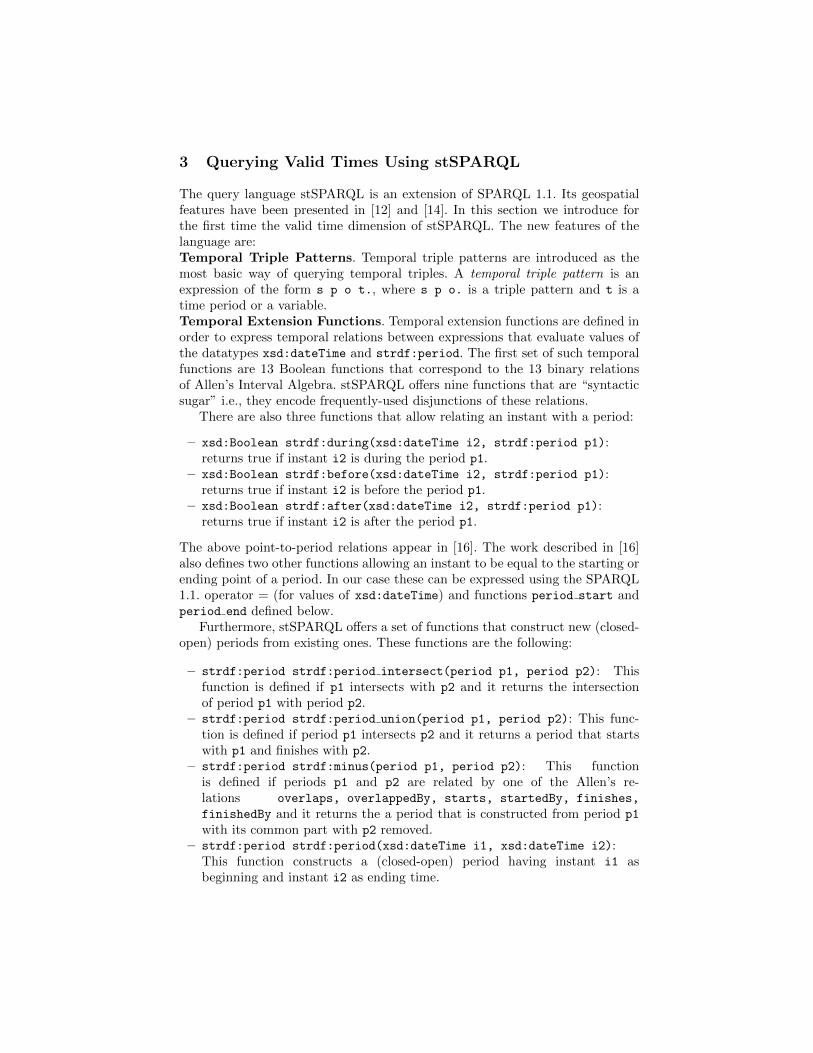
The query language stSPARQL is an extension of SPARQL 1.1. Its geospatialfeatures have been presented in [12] and [14]. In this section we introduce forthe first time the valid time dimension of stSPARQL. The new features of thelanguage are:Temporal Triple Patterns. Temporal triple patterns are introduced as themost basic way of querying temporal triples. A temporal triple pattern is anexpression of the form s p o t., where s p o. is a triple pattern and t is atime period or a variable.Temporal Extension Functions. Temporal extension functions are defined inorder to express temporal relations between expressions that evaluate values ofthe datatypes xsd:dateTime and strdf:period. The first set of such temporalfunctions are 13 Boolean functions that correspond to the 13 binary relationsof Allen’s Interval Algebra. stSPARQL offers nine functions that are “syntacticsugar” i.e., they encode frequently-used disjunctions of these relations.

There are also three functions that allow relating an instant with a period:

– xsd:Boolean strdf:during(xsd:dateTime i2, strdf:period p1):returns true if instant i2 is during the period p1.

– xsd:Boolean strdf:before(xsd:dateTime i2, strdf:period p1):returns true if instant i2 is before the period p1.

– xsd:Boolean strdf:after(xsd:dateTime i2, strdf:period p1):returns true if instant i2 is after the period p1.

The above point-to-period relations appear in [16]. The work described in [16]also defines two other functions allowing an instant to be equal to the starting orending point of a period. In our case these can be expressed using the SPARQL1.1. operator = (for values of xsd:dateTime) and functions period start andperiod end defined below.

Furthermore, stSPARQL offers a set of functions that construct new (closed-open) periods from existing ones. These functions are the following:

– strdf:period strdf:period intersect(period p1, period p2): Thisfunction is defined if p1 intersects with p2 and it returns the intersectionof period p1 with period p2.

– strdf:period strdf:period union(period p1, period p2): This func-tion is defined if period p1 intersects p2 and it returns a period that startswith p1 and finishes with p2.

– strdf:period strdf:minus(period p1, period p2): This functionis defined if periods p1 and p2 are related by one of the Allen’s re-lations overlaps, overlappedBy, starts, startedBy, finishes,

finishedBy and it returns the a period that is constructed from period p1

with its common part with p2 removed.– strdf:period strdf:period(xsd:dateTime i1, xsd:dateTime i2):

This function constructs a (closed-open) period having instant i1 asbeginning and instant i2 as ending time.

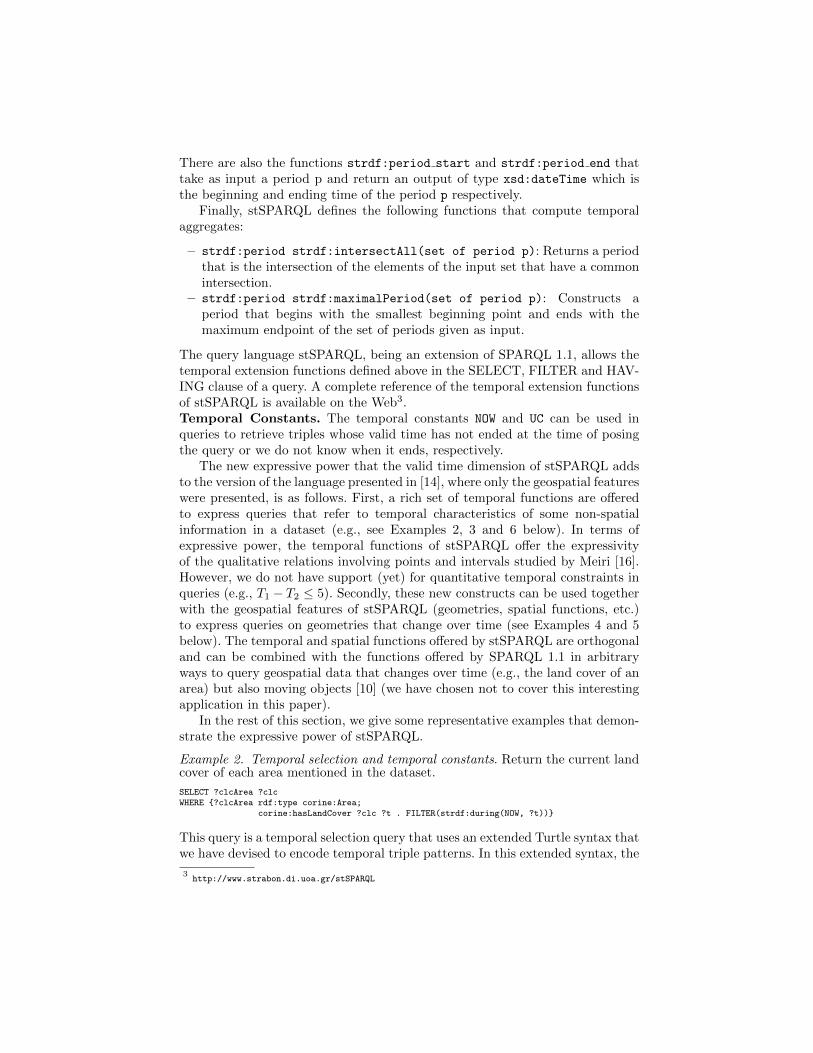
There are also the functions strdf:period start and strdf:period end thattake as input a period p and return an output of type xsd:dateTime which isthe beginning and ending time of the period p respectively.

Finally, stSPARQL defines the following functions that compute temporalaggregates:

– strdf:period strdf:intersectAll(set of period p): Returns a periodthat is the intersection of the elements of the input set that have a commonintersection.

– strdf:period strdf:maximalPeriod(set of period p): Constructs aperiod that begins with the smallest beginning point and ends with themaximum endpoint of the set of periods given as input.

The query language stSPARQL, being an extension of SPARQL 1.1, allows thetemporal extension functions defined above in the SELECT, FILTER and HAV-ING clause of a query. A complete reference of the temporal extension functionsof stSPARQL is available on the Web3.Temporal Constants. The temporal constants NOW and UC can be used inqueries to retrieve triples whose valid time has not ended at the time of posingthe query or we do not know when it ends, respectively.

The new expressive power that the valid time dimension of stSPARQL addsto the version of the language presented in [14], where only the geospatial featureswere presented, is as follows. First, a rich set of temporal functions are offeredto express queries that refer to temporal characteristics of some non-spatialinformation in a dataset (e.g., see Examples 2, 3 and 6 below). In terms ofexpressive power, the temporal functions of stSPARQL offer the expressivityof the qualitative relations involving points and intervals studied by Meiri [16].However, we do not have support (yet) for quantitative temporal constraints inqueries (e.g., T1 − T2 ≤ 5). Secondly, these new constructs can be used togetherwith the geospatial features of stSPARQL (geometries, spatial functions, etc.)to express queries on geometries that change over time (see Examples 4 and 5below). The temporal and spatial functions offered by stSPARQL are orthogonaland can be combined with the functions offered by SPARQL 1.1 in arbitraryways to query geospatial data that changes over time (e.g., the land cover of anarea) but also moving objects [10] (we have chosen not to cover this interestingapplication in this paper).

In the rest of this section, we give some representative examples that demon-strate the expressive power of stSPARQL.

Example 2. Temporal selection and temporal constants. Return the current landcover of each area mentioned in the dataset.

SELECT ?clcArea ?clcWHERE {?clcArea rdf:type corine:Area;

corine:hasLandCover ?clc ?t . FILTER(strdf:during(NOW, ?t))}

This query is a temporal selection query that uses an extended Turtle syntax thatwe have devised to encode temporal triple patterns. In this extended syntax, the

3http://www.strabon.di.uoa.gr/stSPARQL

fourth element is optional and it represents the valid time of the triple pattern.The temporal constant NOW is also used.

Example 3. Temporal selection and temporal join. Give all the areas that wereforests in 1990 and were burned some time after that time.

SELECT ?clcAreaWHERE{?clcArea rdf:type corine:Area ;

corine:hasLandCover corine:ConiferousForest ?t1 ;corine:hasLandCover corine:BurnedArea ?t2 ;FILTER(strdf:during(?t1, "1990-01-01T00:00:00"^^xsd:dateTime) && strdf:after(?t2,?t1))}

This query shows the use of variables and temporal functions to join informationfrom different triples.

Example 4. Temporal join and spatial metric function. Compute the area occu-pied by coniferous forests that were burnt at a later time.

SELECT ?clcArea (SUM(strdf:area(?geo)) AS ?totalArea)WHERE {?clcArea rdf:type corine:Area;

corine:hasLandCover corine:coniferousForest ?t1 ;corine:hasLandCover corine:burntArea ?t2 ;corine:hasGeometry ?geo .

FILTER(strdf:before(?t1,?t2))} GROUP BY ?clcArea

In this query, a temporal join is performed by using the temporal extension func-tion strdf:before to ensure that areas included in the result set were coveredby coniferous forests before they were burnt. The query also uses the spatialmetric function strdf:area in the SELECT clause of the query that computesthe area of a geometry. The aggregate function SUM of SPARQL 1.1 is used tocompute the total area occupied by burnt coniferous forests.

Example 5. Temporal join and spatial selection. Return the evolution of the landcover use of all areas contained in a given polygon.

SELECT ?clc1 ?t1 ?clc2 ?t2WHERE {?clcArea rdf:type corine:Area ;

corine:hasLandCover ?clc1 ?t1 ; corine:hasLandCover ?clc2 ?t2 ;clc:hasGeometry ?geo .

FILTER(strdf:contains(?geo, "POLYGON((-0.66 42.34, ...))"^^strdf:WKT)FILTER(strdf:before(?t1,?t2))}

The query described above performs a temporal join and a spatial selection. Thespatial selection checks whether the geometry of an area is contained in the givenpolygon. The temporal join is used to capture the temporal evolution of the landcover in pairs of periods that preceed one another .

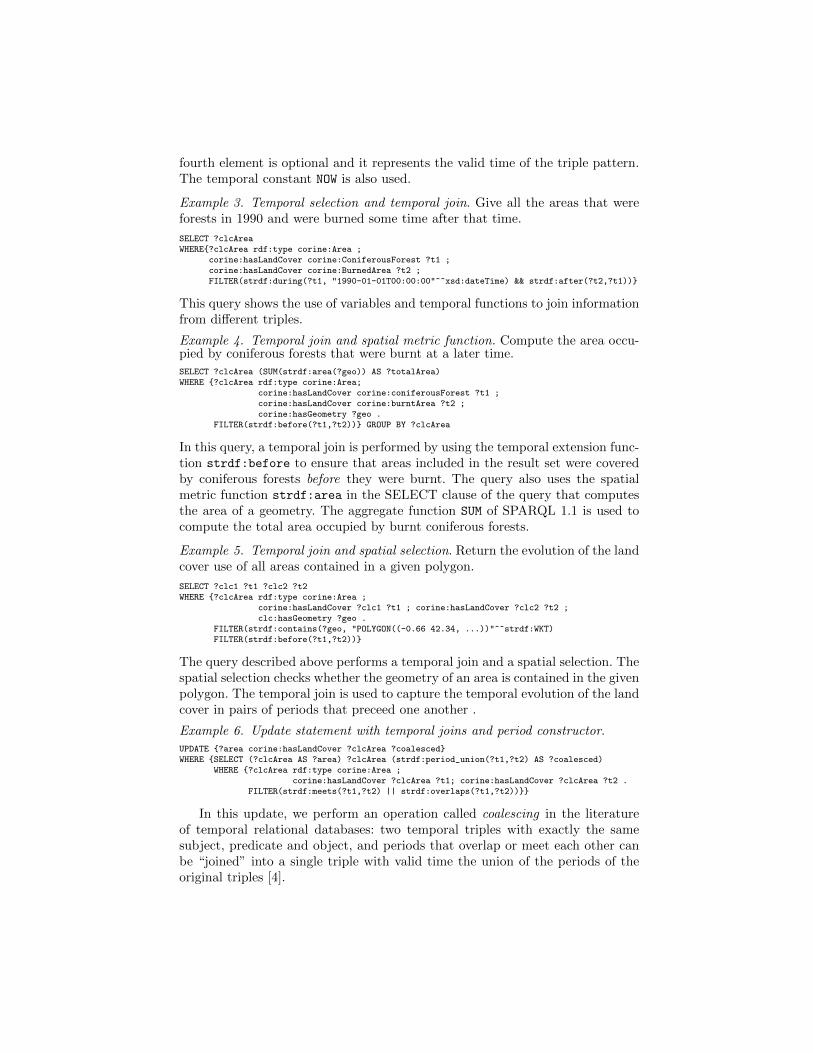
Example 6. Update statement with temporal joins and period constructor.

UPDATE {?area corine:hasLandCover ?clcArea ?coalesced}WHERE {SELECT (?clcArea AS ?area) ?clcArea (strdf:period_union(?t1,?t2) AS ?coalesced)

WHERE {?clcArea rdf:type corine:Area ;corine:hasLandCover ?clcArea ?t1; corine:hasLandCover ?clcArea ?t2 .

FILTER(strdf:meets(?t1,?t2) || strdf:overlaps(?t1,?t2))}}

In this update, we perform an operation called coalescing in the literatureof temporal relational databases: two temporal triples with exactly the samesubject, predicate and object, and periods that overlap or meet each other canbe “joined” into a single triple with valid time the union of the periods of theoriginal triples [4].

Strabon

Repository

SAIL

Query Engine

Parser

Optimizer

Transaction Manager

Storage Manager

RDBMS

Evaluator

stSPARQL to

SPARQL 1.1 Translator

Named Graph

Translator PostgreSQL

MonetDB

GeneralDB

PostGIS

PostgreSQL Temporal

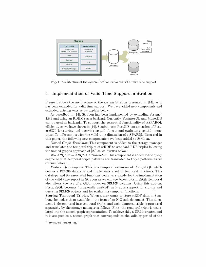
Fig. 1. Architecture of the system Strabon enhanced with valid time support

4 Implementation of Valid Time Support in Strabon

Figure 1 shows the architecture of the system Strabon presented in [14], as ithas been extended for valid time support. We have added new components andextended existing ones as we explain below.

As described in [14], Strabon has been implemented by extending Sesame4

2.6.3 and using an RDBMS as a backend. Currently, PostgreSQL and MonetDBcan be used as backends. To support the geospatial functionality of stSPARQLefficiently as we have shown in [14], Strabon uses PostGIS, an extension of Post-greSQL for storing and querying spatial objects and evaluating spatial opera-tions. To offer support for the valid time dimension of stSPARQL discussed inthis paper, the following new components have been added to Strabon.

Named Graph Translator. This component is added to the storage managerand translates the temporal triples of stRDF to standard RDF triples followingthe named graphs approach of [22] as we discuss below.

stSPARQL to SPARQL 1.1 Translator. This component is added to the queryengine so that temporal triple patterns are translated to triple patterns as wediscuss below.

PostgreSQL Temporal. This is a temporal extension of PostgreSQL whichdefines a PERIOD datatype and implements a set of temporal functions. Thisdatatype and its associated functions come very handy for the implementationof the valid time suport in Strabon as we will see below. PostgreSQL Temporalalso allows the use of a GiST index on PERIOD columns. Using this add-on,PostgreSQL becomes “temporally enabled” as it adds support for storing andquerying PERIOD objects and for evaluating temporal functions.Storing Temporal Triples. When a user wants to store stRDF data in Stra-bon, she makes them available in the form of an N-Quads document. This docu-ment is decomposed into temporal triples and each temporal triple is processedseparately by the storage manager as follows. First, the temporal triple is trans-lated into the named graph representation. To achieve this, a URI is created andit is assigned to a named graph that corrresponds to the validity period of the

4http://www.openrdf.org/

triple. To ensure that every distinct valid time of a temporal triple correspondsto exactly one named graph, the URI of the graph is constructed using the literalrepresentation of the valid time annotation. Then, the stored triple in the namedgraph identified by this URI and the URI of the named graph is associated toits corresponding valid time by storing the following triple in the default graph:(g, strdf:hasValidTime, t) where g is the URI of the graph and t is thecorresponding valid time. For example, temporal triple

corine:Area_4 corine:hasLandCover corine:naturalGrassland"[2000-01-01T00:00:00,2006-01-01T00:00:00)"^^strdf:period

will be translated into the following standard RDF triples:

corine:Area_4 corine:hasLandCover corine:naturalGrasslandcorine:2000-01-01T00:00:00_2006-01-01T00:00:00 strdf:hasValidTime

"[2000-01-01T00:00:00,2006-01-01T00:00:00)"^^strdf:period

The first triple will be stored in the named graph with URIcorine:2000-01-01T00:00:00_2006-01-01T00:00:00 and the second in the default graph. Iflater on another temporal triple with the same valid time is stored, its corre-sponding triple will end-up in the same named graph.

For the temporal literals found during data loading, we deviate from the de-fault behaviour of Sesame by storing the instances of the strdf:period datatypein a table with schema period values(id int, value period). The attribute id isused to assign a unique identifier to each period and associate it to its RDFrepresentation as a typed literal. It corresponds to the respective id value that isassigned to each URI after the dictionary encoding is performed. The attributevalue is a temporal column of the PERIOD datatype defined in PostgreSQL Tem-poral. In addition, we construct a GiST index on the value column.

Querying Temporal Triples. Let us now explain how the query engine of Stra-bon presented in [14] has been extended to evaluate temporal triple patterns.When a temporal triple pattern is encountered, the query engine of Strabonexecutes the following steps. First, the stSPARQL to SPARQL 1.1 Translatorconverts each temporal triple pattern of the form s p o t into the graph pat-tern GRAPH ?g s p o . ?g strdf:hasValidTime t. where s, p, o are RDFterms or variables and t is either a variable or an instance of the datatypesstrdf:period or xsd:dateTime. Then the query gets parsed and optimized bythe respective components of Strabon and passes to the evaluator which has beenmodified as follows: If a temporal extension function is present, the evaluatorincorporates the table period values to the query tree and it is declared that thearguments of the temporal function will be retrieved from the period values table.In this way, all temporal extension functions are evaluated in the database levelusing PostgresSQL Temporal. Finally, the RDBMS evaluation module has beenextended so that the execution plan produced by the logical level of Strabonis translated into suitable SQL statements. The temporal extension functionsare respectively mapped into SQL statements using the functions and operatorsprovided by PostgreSQL Temporal.

5 Evaluation

For the experimental evaluation of our system, we used two different datasets.The first dataset is the GovTrack dataset5, which consists of RDF data aboutUS Congress. This dataset was created by Civic Impulse, LLC6 and containsinformation about US Congress members, bills and voting records. The seconddataset is the CORINE Land Cover changes dataset that represents changes forthe period [2000, UC), which we have already introduced in Section 2.

The GovTrack dataset contains temporal information in the form of instantsand periods, but in standard RDF format using reification. So, in the pre-processing step we transformed the dataset into N-Quads format. For examplethe 5 triples

congress_people:A000069 politico:hasRole _:node17d3oolkdx1 ._:node17d3oolkdx1 time:from _:node17d3oolkdx2 ._:node17d3oolkdx1 time:to _:node17d3oolkdx3 ._:node17d3oolkdx2 time:at "2001-01-03"^^xs:date ._:node17d3oolkdx3 time:at "2006-12-08"^^xs:date .

were transformed into a single quad:

congress_people:A000069 politico:hasRole _:node17d3oolkdx1"[2001-01-03T00:00:00, 2006-12-08T00:00:00]"^^strdf:period .

The transformed dataset has a total number of 7,900,905 triples, 42,049 ofwhich have periods as valid time and 294,636 have instants.

The CORINE Land Cover changes dataset for the time period [2000, UC) ispublicly available in the form of shapefiles and it contains the areas that havechanged their land cover between the years 2000 and 2006. Using this dataset,we created a new dataset in N-Quads form which has information about geo-graphic regions such as: unique identifiers, geometries and periods when regionshave a landcover. The dataset contains 717,934 temporal triples whose validtime is represented using the strdf:period datatype. It also contains 1,076,901triples without valid times. Using this dataset, we performed temporal and spa-tial stSPARQL queries, similar to the ones provided in Section 3 as examples.

Our experiments were conducted on an Intel Xeon E5620 with 12MB L3caches running at 2.4 GHz. The system has 24GB of RAM, 4 disks of stripedRAID (level 5) and the operating system installed is Ubuntu 12.04. We ran ourqueries three times on cold and warm caches, for which we ran each query oncebefore measuring the response time. We compare our system with the followingimplementations.The Prolog-based implementation of AnQL. We disabled the inferencer and wefollowed the data model and the query language that is used in [15], e.g., theabove quad is transformed into the following AnQL statement:

congress_people:A000069 politico:hasRole _:node1 :[2001-01-03, 2006-12-08] .

5http://www.govtrack.us/data/rdf/

6http://www.civicimpulse.com/

AllegroGraph. AllegroGraph offers a set of temporal primitives and temporalfunctions, extending their Prolog query engine, to represent and query temporalinformation in RDF. AllegroGraph does not provide any high level syntax toannotate triples with their valid time, so, for example, the GovTrack triple thatwe presented earlier was converted into the following graph:

congress_people:A000069 politico:hasRole _:node1 graph:2001-01-03T... .graph:2001-01-03T... allegro:starttime "2001-01-03T00:00:00"^^xsd:dateTime .graph:2001-01-03T... allegro:endtime "2001-01-03T00:00:00"^^xsd:dateTime .

As AllegroGraph supports the N-Quads format, we stored each triple of thedataset in a named graph, by assigning a unique URI to each valid time. Then,we described the beginning and ending times of the period that the named graphcorresponds to, using RDF statements with the specific temporal predicates thatare defined in AllegroGraph7. We used the AllegroGraph Free server edition8

that allows us to store up to five million statements, so we could not store thefull version of the dataset.Naive implementation. We developed a baseline implementation by extendingthe Sesame native store with the named graph translators we use in Strabon sothat it can store stRDF graphs and query them using stSPARQL queries. Wealso developed in Java the temporal extension functions that are used in thebenchmarks. A similar implementation has been used as a baseline in [14] wherewe evaluated the geospatial features of Strabon.

We evaluate the performance of the systems in terms of query response time.We compute the response time for each query posed by measuring the elapsedtime from query submission till a complete iteration over the results had beencompleted. We also investigate the scalability with respect to database size andcomplexity of queries.

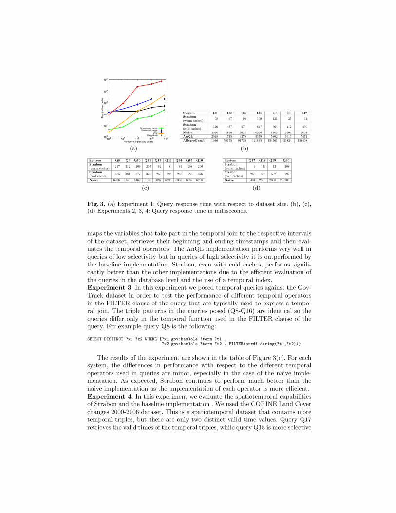
We have conducted four experiments that are explained below. Twenty querieswere used in the evaluation. Only two queries are shown here; the rest are omit-ted due to space considerations. However, all datasets and the queries that weused in our experimental evaluation are publicly available9.Experiment 1. In this experiment we ran the same query against a numberof subsets of the GovTrack dataset of various size, as we wanted to test thescalability of all systems with respect to the dataset size. To achieve this, wecreated five instances of the GovTrack dataset, each one with exponentiallyincreasing number of triples and quads. The query that is evaluated againstthese datasets is shown in Figure 2.

Figure 3(a) shows the results of this experiment. As the dataset size increases,more periods need to be processed and as expected, the query response timegrows for all systems. This is expected, as posing queries against a large datasetis challenging for memory-based implementations. Interestingly, the AnQL re-sponse time in the query Q2 is decreased, when a temporal filter is added to thetemporal graph pattern of the query Q1. The use of a very selective temporal

7http://www.franz.com/agraph/support/documentation/current/temporal-tutorial.html

8http://www.franz.com/agraph/downloads/

9http://www.strabon.di.uoa.gr/temporal-evaluation/experiments.html

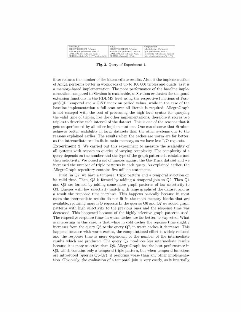
stSPARQL AnQL AllegroGraphSELECT DISTINCT ?x ?name SELECT DISTINCT ?x ?name (select0-distinct (?x ?name)WHERE {?x gov:hasRole ?term ?t . WHERE {?x gov:hasRole ?term ?t . (q ?x !gov:hasRole ?term ?t)OPTIONAL {?x foaf:name ?name .} OPTIONAL {?x foaf:name ?name .} (optional (q ?x !foaf:name ?name))FILTER(strdf:after(?t,“[...]”ˆˆstrdf:period))} FILTER(beforeany([[...]],?t))} (interval-after-datetimes ?t “...”))

Fig. 2. Query of Experiment 1.

filter reduces the number of the intermediate results. Also, it the implementationof AnQL performs better in workloads of up to 100,000 triples and quads, as it isa memory-based implementation. The poor performance of the baseline imple-mentation compared to Strabon is reasonable, as Strabon evaluates the temporalextension functions in the RDBMS level using the respective functions of Post-greSQL Temporal and a GiST index on period values, while in the case of thebaseline implementation a full scan over all literals is required. AllegroGraphis not charged with the cost of processing the high level syntax for queryingthe valid time of triples, like the other implementations, therefore it stores twotriples to describe each interval of the dataset. This is one of the reasons that itgets outperformed by all other implementations. One can observe that Strabonachieves better scalability in large datasets than the other systems due to thereasons explained earlier. The results when the caches are warm are far better,as the intermediate results fit in main memory, so we have less I/O requests.

Experiment 2. We carried out this experiment to measure the scalability ofall systems with respect to queries of varying complexity. The complexity of aquery depends on the number and the type of the graph patterns it contains andtheir selectivity. We posed a set of queries against the GovTrack dataset and weincreased the number of triple patterns in each query. As explained earlier, theAllegroGraph repository contains five million statements.

First, in Q2, we have a temporal triple pattern and a temporal selection onits valid time. Then, Q3 is formed by adding a temporal join to Q2. Then Q4and Q5 are formed by adding some more graph patterns of low selectivity toQ3. Queries with low selectivity match with large graphs of the dataset and asa result the response time increases. This happens basically because in mostcases the intermediate results do not fit in the main memory blocks that areavailable, requiring more I/O requests In the queries Q6 and Q7 we added graphpatterns with high selectivity to the previous ones and the response time wasdecreased. This happened because of the highly selective graph patterns used.The respective response times in warm caches are far better, as expected. Whatis interesting in this case, is that while in cold caches the reponse time slightlyincreases from the query Q6 to the query Q7, in warm caches it decreases. Thishappens because with warm caches, the computational effort is widely reducedand the response time is more dependent of the number of the intermediateresults which are produced. The query Q7 produces less intermediate resultsbecause it is more selective than Q6. AllegroGraph has the best performance inQ2, which contains only a temporal triple pattern, but when temporal functionsare introduced (queries Q3-Q7), it performs worse than any other implementa-tion. Obviously, the evaluation of a temporal join is very costly, as it internally

100

101

102

103

104

105

103

104

105

106

107

Tim

e (

mill

iseconds)

Number of triples and quads

Strabon(warm cache)Strabon(cold cache)

NaiveAnQL

AllegroGraph

(a)

System Q1 Q2 Q3 Q4 Q5 Q6 Q7Strabon

98 67 92 109 131 35 31(warm caches)Strabon

326 437 571 647 664 412 430(cold caches)Naive 3056 5860 5916 6260 6462 2594 2604AnQL 2028 1715 4275 4379 5802 6913 7472AllegroGraph 1016 58155 91736 121835 154561 33824 156408

(b)

System Q8 Q9 Q10 Q11 Q12 Q13 Q14 Q15 Q16Strabon

217 212 209 207 82 84 81 208 200(warm caches)Strabon

485 381 377 370 250 248 248 285 376(cold caches)Naive 6206 6148 6162 6196 6097 6248 6388 6332 6258

(c)

System Q17 Q18 Q19 Q20Strabon

3 13 12 208(warm caches)Strabon

268 368 532 792(cold caches)Naive 404 2868 2388 200705

(d)

Fig. 3. (a) Experiment 1: Query response time with respect to dataset size. (b), (c),(d) Experiments 2, 3, 4: Query response time in milliseconds.

maps the variables that take part in the temporal join to the respective intervalsof the dataset, retrieves their beginning and ending timestamps and then eval-uates the temporal operators. The AnQL implementation performs very well inqueries of low selectivity but in queries of high selectivity it is outperformed bythe baseline implementation. Strabon, even with cold caches, performs signifi-cantly better than the other implementations due to the efficient evaluation ofthe queries in the database level and the use of a temporal index.Experiment 3. In this experiment we posed temporal queries against the Gov-Track dataset in order to test the performance of different temporal operatorsin the FILTER clause of the query that are typically used to express a tempo-ral join. The triple patterns in the queries posed (Q8-Q16) are identical so thequeries differ only in the temporal function used in the FILTER clause of thequery. For example query Q8 is the following:

SELECT DISTINCT ?x1 ?x2 WHERE {?x1 gov:hasRole ?term ?t1 .?x2 gov:hasRole ?term ?t2 . FILTER(strdf:during(?t1,?t2))}

The results of the experiment are shown in the table of Figure 3(c). For eachsystem, the differences in performance with respect to the different temporaloperators used in queries are minor, especially in the case of the naive imple-mentation. As expected, Strabon continues to perform much better than thenaive implementation as the implementation of each operator is more efficient.Experiment 4. In this experiment we evaluate the spatiotemporal capabilitiesof Strabon and the baseline implementation . We used the CORINE Land Coverchanges 2000-2006 dataset. This is a spatiotemporal dataset that contains moretemporal triples, but there are only two distinct valid time values. Query Q17retrieves the valid times of the temporal triples, while query Q18 is more selective

and performs a temporal join. Query Q19 is similar to Q20 but it also retrievesgeospatial information so the response time is increased. Query 20 performs atemporal join and a spatial selection, so the reponse time is increased for bothsystems. Strabon peforms better because the temporal and the spatial operationsare evaluated in the database level and the respective indices are used, while inthe naive implementation these functions are implemented in Java.

6 Related Work

To the best of our knowledge, the only commercial RDF store that has goodsupport for time is AllegroGraph10. AllegroGraph allows the introduction ofpoints and intervals as resources in an RDF graph and their situation on a timeline (by connecting them to dates). It also offers a rich set of predicates thatcan be used to query temporal RDF graphs in Prolog. As in stSPARQL, thesepredicates include all qualitative relations of [16] involving points and intervals.Therefore, all the temporal queries expressed using Prolog in AllegroGraph canalso be expressed by stSPARQL in Strabon.

In [7] another approach is presented for extending RDF with temporal fea-tures, using a temporal element that captures more than one time dimensions.A temporal extension of SPARQL, named T -SPARQL, is also proposed which isbased on TSQL2. Also, [17] presents a logic-based approach for extending RDFand OWL with valid time and the query language SPARQL for querying andreasoning with RDF, RDFS and OWL2 temporal graphs. To the best of ourknowledge, no public implementation of [7] and [17] exists that we could use tocompare with Strabon. Similarly, the implementations of [19] and [22] are notpublicly available, so they could not be included in our comparison.

In stRDF we have not considered transaction time since the applications thatmotivated our work required only user-defined time and valid time of triples.The introduction of transaction time to stRDF would result in a much richerdata model. We would be able to model not just the history of an applicationdomain, but also the system’s knowledge of this history. In the past the relevantrich semantic notions were studied in TSQL2 [20], Telos (which is very close toRDF) [18] and temporal deductive databases [21].

7 Conclusions

In future work, we plan to evaluate the valid time functionalities of Strabon onlarger datasets, and continue the experimental comparison with AllegroGraphas soon as we obtain a license of its Enterprise edition. We will also study opti-mization techniques that can increase the scalability of Strabon. Finally, it wouldbe interesting to define and implement an extension of stSPARQL that offersthe ability to represent and reason with qualitative temporal relations in thesame way that the Topology vocabulary extension of GeoSPARQL representstopological relations.

10http://www.franz.com/agraph/allegrograph/

References

1. Open Geospatial Consortium. OGC GeoSPARQL - A geographic query languagefor RDF data. OGC Candidate Implementation Standard (2012)

2. Al-Kateb, M., Ghazal, A., Crolotte, A., Bhashyam, R., Chimanchode, J., Pakala,S.P.: Temporal Query Processing in Teradata. In: ICDT (2013)

3. Allen, J.F.: Maintaining knowledge about temporal intervals. CACM 26(11) (1983)4. Boelen, M.H., Snodgrass, R.T., Soo, M.D.: Coalescing in Temporal Databases.

IEEE CS 19, 35–42 (1996)5. Clifford, J., Dyreson, C., Isakowitz, T., Jensen, C.S., Snodgrass, R.T.: On the

semantics of now in databases. ACM TODS 22(2), 171–214 (1997)6. Date, C.J., Darwen, H., Lorentzos, N.A.: Temporal data and the relational model.

Elsevier (2002)7. Grandi, F.: T-SPARQL: a TSQL2-like temporal query language for RDF. In: In-

ternational Workshop on Querying Graph Structured Data. pp. 21–30 (2010)8. Gutierrez, C., Hurtado, C., Vaisman, R.: Temporal RDF. In: Gmez-Prez, A., Eu-

zenat, J. (eds.) ESWC. LNCS, vol. 3532, pp. 93–107. Springer (2005)9. Gutierrez, C., Hurtado, C.A., Vaisman, A.: Introducing Time into RDF. IEEE

TKDE 19(2), 207–218 (2007)10. Guting, R.H., Bohlen, M.H., Erwig, M., Jensen, C.S., Lorentzos, N.A., Schneider,

M., Vazirgiannis, M.: A foundation for representing and querying moving objects.ACM TODS 25(1), 1–42 (2000)

11. Hurtado, C.A., Vaisman, A.A.: Reasoning with Temporal Constraints in RDF. In:Alferes, J., Bailey, J., May, W., Schwertel, U. (eds.) PPSWR. LNCS, vol. 4187, pp.164–178. Springer (2006)

12. Koubarakis, M., Karpathiotakis, M., Kyzirakos, K., Nikolaou, C., Sioutis, M.: DataModels and Query Languages for Linked Geospatial Data. In: Eiter, T., Krennwall-ner, T. (eds.) RR. LNCS, vol. 7487, pp. 290–328. Springer (2012)

13. Koubarakis, M., Kyzirakos, K.: Modeling and Querying Metadata in the SemanticSensor Web: The Model stRDF and the Query Language stSPARQL. In: Aroyo,L., et al. (eds.) ESWC. LNCS, vol. 6088, pp. 425–439. Springer (2010)

14. Kyzirakos, K., Karpathiotakis, M., Koubarakis, M.: Strabon: A Semantic Geospa-tial DBMS. In: Cudr-Mauroux, P., et al. (eds.) ISWC. LNCS, vol. 7649, pp. 295–311. Springer (2012)

15. Lopes, N., Polleres, A., Straccia, U., Zimmermann, A.: AnQL: SPARQLing UpAnnotated RDFS. In: Patel-Schneider, P., et al. (eds.) ISWC. LNCS, vol. 6496.Springer (2010)

16. Meiri, I.: Combining qualitative and quantitative constraints in temporal reasoning.Artificial Intelligence 87(1-2), 343–385 (1996)

17. Motik, B.: Representing and Querying Validity Time in RDF and OWL: A Logic-Based Approach. Journal of Web Semantics 12–13, 3–21 (2012)

18. Mylopoulos, J., Borgida, A., Jarke, M., Koubarakis, M.: Telos: representing knowl-edge about information systems. ACM TIS (1990)

19. Perry, M.: A Framework to Support Spatial, Temporal and Thematic Analyticsover Semantic Web Data. Ph.D. thesis, Wright State University (2008)

20. Snodgrass, R.T. (ed.): The TSQL2 Temporal Query Language. Springer (1995)21. Sripada, S.M.: A logical framework for temporal deductive databases. In: Bancil-

hon, F., DeWitt, D. (eds.) VLDB. pp. 171–182. M. Kaufmann Publ. Inc. (1988)22. Tappolet, J., Bernstein, A.: Applied Temporal RDF: Efficient Temporal Querying

of RDF Data with SPARQL. In: Aroyo, L., et al. (eds.) ESWC. LNCS, vol. 5554,pp. 308–322. Springer-Verlag (2009)