Report - USNA stuff/Report... · Report SM495 Meredith Lipp ... Stimulated Emission, Photon Amplification, and Lasers ... by S. O. Kasap, New York, 2013. Lipp 12

UNITED STATES NAVAL ACADEMY

Report SM495

Meredith Lipp

12/18/2013

Lipp 1

Table of Contents

Introduction………………………………………………………………………………… 2

Motivation………………………………………………………………………………..… 3

Background Knowledge………………………………………………………...………… 5

History………………………………………………………………………….….…. 5

Stimulated Emission, Photon Amplification, and Lasers………………………..….... 11

Helium-Neon Laser………………………………….………………...………….….. 12

Related Paper Analysis………………………………...……………………….………… 14

Pseudo-Partially Coherent Beam for Free-Space Laser Communication…………… 14

Numerical Investigation on Propagation Effects of Pseudo-Partially Coherent

Gaussian Schell-model Beam in Atmospheric Turbulence…………………………… 15

Convolution Project……………………………………………..….………………..…… 16

Sinusoidal Input with Noise through Low Pass Filter...……………………………… 16

Two Sinusoidal Inputs through Low Pass Filter..……………………………………. 19

Sinusoidal Input with Noise through High Pass Filter...........................……….....…. 20

Two Sinusoidal Inputs through High Pass Filter ………….…...…….…………….... 21

Conclusion……………………………………………………………………………. 21

Research Summary…………………………………..……………….………………….... 22

Equipment.……………….……….………………………………………….…………. 23

Emulator Setup……….…………………………………………………….………....... 23

Laser, Expander, and SLM Setup…………….………………………………………… 25

SLM Screens………….……….………………………………………………………… 25

Process.……………….……….…………………………………………………..……. 26

Results ………….……….……………………………………………………………… 26

Conclusion....……………….……….………………………………………………….. 27

References…………………………………...……………..………………….…………… 28

Appendix……………..……………………...……………..………………….…………… 29

Lipp 2

Introduction

The purpose of this course is to provide background knowledge on laser beam

propagation as well as conduct experiments oriented toward the ultimate goal of improving laser

propagation through the maritime environment. Lasers can be a useful tool for remote sensing,

communications, and as a weapon. However, because of the effects air turbulence has on a beam,

using lasers in these areas has not yet been utilized to its full potential. Turbulence results in

decreased intensity at the target in addition to increased scintillation (the amount a beam varies at

a point). By possible manipulations to a beam at the source, we hope to achieve increased

intensity at the target with decreased scintillation.

Lipp 3

Motivation

As mentioned above, the purpose of this project is to produce a method that will allow

laser beams to propagate through a maritime environment with minimal scintillation and little

reduction in intensity. This new technique could then be applied as a way to communicate long

distances or as a weapon. Recently, I discussed with a researcher how this type of system would

be useful on a submarine. When a submarine surfaces, it is extremely vulnerable to attack by

helicopters. Therefore, utilizing a laser targeting system would reduce its vulnerability so that the

aircraft could be brought down more quickly. There are many more applications within the

military, but this is just one example. Research in this area is being pursued fervently all around

the country, and the world as well.

Personally, I was introduced to this research when my cousin, who attended the United

States Naval Academy and graduated in 2010, encouraged me to take an Introduction to Laser

Research course the second semester of my freshman year. I then became an assistant to a 1/C

midshipman who was conducting his research in laser propagation and was introduced to

Professor Avramov, Assistant Professor Nelson, and Professor Malek-Madani. Over the course

of the semester, I became familiar with the equipment being used to conduct the research. Also,

the classroom sessions introduced some of the mathematics involved with lasers and how it can

be applied to real world scenarios. However, this research focuses on what happens when

mathematics can no longer exactly predict what will happen because the environment through

which the laser is propagating is not ideal. I am extremely interested in lasers because I can

directly see the results of my research and how it will eventually be applied on a large scale.

Technically, this problem interests me because there are so many factors to consider. We

have the tools to measure the atmospheric conditions and manipulate the beams. However, we

Lipp 4

only need to find the correct algorithm to allow the beam to propagate successfully. I hope that

my time at the Academy will continue moving toward this goal and allow others to build off of

my research to eventually reach a solution.

In my 1/C year, I would like to participate in the Trident Research Scholarship Program

which would allow me to devote an entire year to an extensive research project in this field. In

addition, I see the possibility of pursuing a master’s degree after graduation from the Naval

Academy and continuing my research.

Lipp 5

Background Knowledge

In lectures with Professor Nelson, I am gaining an understanding of basic laser operations

and the different theories which have led to the current understanding of the atomic orbitals and

laser propagation.

History

1885

- Balmer discovers that the hydrogen atom has discrete energy levels

1900

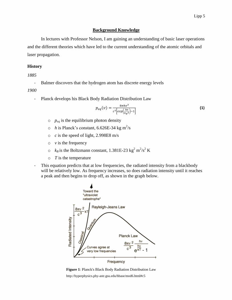
- Planck develops his Black Body Radiation Distribution Law

( )

[ (

) ]

(1)

o peq is the equilibrium photon density

o h is Planck’s constant, 6.626E-34 kg m2/s

o c is the speed of light, 2.998E8 m/s

o v is the frequency

o kB is the Boltzmann constant, 1.381E-23 kg2 m

2/s

2 K

o T is the temperature

- This equation predicts that at low frequencies, the radiated intensity from a blackbody

will be relatively low. As frequency increases, so does radiation intensity until it reaches

a peak and then begins to drop off, as shown in the graph below.

Figure 1: Planck's Black Body Radiation Distribution Law

http://hyperphysics.phy-astr.gsu.edu/hbase/mod6.html#c5

Lipp 6

1905

- Einstein defines the photoelectric effect

o

“photons”

Figure 2: (a) The photoelectric effect (b) the maximum kinetic energy of the

photoelectron as a function of incident frequency.

“Laser Fundamentals,” 2nd edition, by William T. Silfvast, Cambridge, 2004.

3 Key Ideas:

1. The first key idea of quantum mechanics was given by Planck who described the atom as

having discrete energy levels which produced photons of light, which he called quanta.

2. Next, Einstein identified the wave-particle duality of light, demonstrating how it possessed

wave-like properties by diffraction but particle-like properties in delivery of discrete packets of

energy, called photons.

Figure 3: Double-slit diffraction pattern for electrons emitted from an electron

gun, showing the pattern obtained when passing through each individual slit

and then the pattern with both slits.

“Laser Fundamentals,” 2nd edition, by William T. Silfvast, Cambridge, 2004.

Lipp 7

3. Finally, Heisenberg outlined his Uncertainty Principle, stating that we could never know both

how fast an electron is moving and where it is at the same time.

These 3 key ideas are the building blocks of quantum mechanics and are crucial to our

understanding of light and lasers.

1913

- Bohr uses classical physics to define atomic orbitals

o Assumes there is a mass at the center with electrons orbiting

o

(2)

The n indicates that there can only be certain energy levels

o (3)

This is a photon of energy

( )

(4)

is the first Bohr radius

o

defines energy for each atomic orbital

Lipp 8

1924

- DeBroglie introduces the idea of matter waves

(relativistic parameter)

As v approaches c, goes to

(5)

1926

- Schrodinger’s Equation (6)

o Published by Erwin Schrodinger in 1926, this equation is a linear partial

differential equation which describes the wave function of a system, also known

as the quantum state.

o Solutions to this equation can be used to describe many systems; however, in this

case, we are using it to describe the discrete energy levels found in the atom.

o Building on DeBroglie’s idea of matter waves, the solution reveals that the

frequency of a particle is directly proportional to the total energy (7) of a system.

Lipp 9

- Infinite Potential Well Example

o This illustration supposes that there is a particle in free space surrounded by

impenetrable barriers. As the space becomes narrower, the particle will only be

found in certain places since it can only occupy certain energy levels.

o This model is one of the simplest since it can be solved using the mass of the

particle and width of the well. It gives insight into quantum mechanics without

complex mathematics.

o Equation 8 is the result of the infinite potential well example using the

Schrodinger equation and initial conditions.

∞ ∞

Region 1 Region 2 Region 3

V(x)

x = 0 x = a

Figure 4: Potential Function of the infinite potential well.

“Semiconductor Physics and Devices,” 3rd edition, by Donald A.

Neamen, McGraw Hill, 2003.

Lipp 10

( )

( ) ( )

( )

(6)

( ) ( ) ( )

( )

( ( )) ( )

( ) ( ) ( )

( ) ( ) ( )

( ) ( ) ( )

∫ ( ( ))

√

( ) √

(

) (7)

√

(

)

(8)

Lipp 11

Stimulated Emission, Photon Amplification, and Lasers

As demonstrated above, if an electron absorbs a photon of energy, it can be excited from

a lower energy state (E1) to a higher energy state (E2). Then, when the electrontransfers from its

excited state, it emits a photon equal to the change in energy level (E2 – E1 = hv). This process

usually occurs spontaneously, or it can be induced by another photon. This is called stimulated

emission and is the foundation upon which laser principles are based. When an excited electron

is hit with a photon with energy E2 – E1 = hv, the electron transits from E2 to E1. Population

inversion is when more electrons are at E2 than E1; however, three energy states are required for

this to occur. Using the ruby laser as an example, electrons are stimulated to the third energy

level with photons = E3 – E1 = hv3. This is called pumping. From E3, the electrons spontaneously

transition to E2, which is known as a metastable state in which the electrons can exist for a

relatively long period of time before they transfer to E1. Therefore, the electrons accumulate at

E2 causing a population inversion. When one electron spontaneously decays to E1, it causes the

other electrons in E2 to also decay, emitting light as a large collection of coherent photons. This

emission is called the lasing emission. This entire process describes photon amplification, and

the device which accomplishes this is a laser, an acronym for Light Amplification by Stimulated

Emission of Radiation.

Figure 5: Light Amplification by Stimulated Emission of Radiation

“Optoelectronics and Photonics, Principles and Practices,” 2nd edition, by S. O. Kasap, New York, 2013.

Lipp 12

Helium-Neon (He-Ne) Laser

The ruby laser is a relatively simple version of a laser; however a Helium-Neon laser,

which actually has four energy levels, is used in our research. The helium atoms are excited to a

higher energy state which then excites the neon atoms to a metastable state. The electrons are

then induced to fall to a lower energy level and emit coherent light. This process emits light at

632.8 nm, giving the He-Ne laser its well-known red color. This is demonstrated in Figure 6

below.

Figure 6: The principles of operation of the He-Ne laser and the He-Ne laser energy levels

involved for 632.8 nm emission.

“Optoelectronics and Photonics, Principles and Practices,” 2nd edition, by S. O. Kasap, New York, 2013.

Lipp 13

While the internal process has been discussed in detail, the actual assembly of the He-Ne

laser is very intricate as well. A typical He-Ne laser contains a helium and neon gas mixture

within a narrow glass tube and the ends are sealed with a flat mirror on one end and a concave

mirror at the other, forming an optical cavity. This emits a Gaussian beam.

Figure 7: Functionality of a laser

“Introduction to Optics,” 3rd edition, by Pedrotti, Pedrotti and Pedrotti, Pearson, 2007.

Lipp 14

Related Paper Analysis

I have read numerous papers about laser beam propagation. Included below are

summaries of the ones which focus on what have come to be known as pseudo-partially coherent

beams (PPCBs).

Pseudo-Partially Coherent Beam for Free-Space Laser Communication

David Voelz and Kevin Fitzhenry

This paper describes a process to “modulate or temporally alter the phase front of the

beam before transmission” which would reduce scintillation at the target and improve the use of

a laser for communication purposes. The research seeks to minimize scintillation and beam

spread so that a large receiver is not required to detect the beam. Scintillation arises from

atmospheric turbulence which disrupts the laser beam. This paper theorizes that by sending many

different beams very quickly through the turbulence, at the receiver the entire beam will be

“filled in” per say. The results from this paper discuss that while manipulation of the beam

caused greater spread, the results of scintillation were reduced.

This paper directly applies to our research because by using the SLM we can alter the

phase of the laser beam creating a different beam which will hopefully propagate through the

atmosphere better than the original. Presently, we are exploring the idea of cycling, using 4000

screens produced by MATLAB with different degrees of correlation. Using Far Field

Transforms, we can predict the outcome of the beam and are looking into propagating “flat top”

beams which are more spread out over a larger region rather than having the standard high

intensity point in the center. Therefore, these beams have a higher probability of reaching a

certain intensity at the target, which could then be translated into a message of some kind. This

paper discusses cycling, which in combination with the flat top beam, could prove very

successful at propagating through the atmosphere and resisting its effects.

Lipp 15

Numerical Investigation on Propagation Effects of Pseudo-Partially Coherent Gaussian

Schell-model Beam in Atmospheric Turbulence

Xianmei Qian, Wenyue Zhu and Ruizhong Rao

Similar to the previous paper, this discusses the effects of Pseudo Partially Coherent

Beams (PPCBs) and their advantages and disadvantages over coherent beams. PPCBs use the

theory that during the period that the atmosphere has changed once, the phase screen has cycled

multiple times. This paper found that the beam radius of a PPCB is always larger than a Coherent

Beam (CB) in free space and turbulence. However, the beam radius of a PPCB is the same in

turbulence as free space, whereas the CB beam radius is changed based on the atmosphere. Thus,

partially coherent beams are less affected by atmospheric turbulence than coherent beams. The

paper also reveals that the beam wander of the CB is larger than that of a PPCB; however, the

difference is very slight. Interestingly, the scintillation index of a PPCB is lower than that of a

CB, which is the goal of our research. Therefore, this suggests that PPCBs are more resistant to

the influences of a turbulent atmosphere, such as that found in the maritime environment.

Finally, since PPCBs do have larger beam spread than CBs, this would result in a larger

dispersion of energy. Thus, there must be a balance between intensity delivered and lower

scintillation.

Lipp 16

Convolution Project

The design goal of this project is to reduce the amount of noise or the influence of the

unwanted signal at the output. Two types of filters are suggested for consideration. The code for

this project is referenced in the Appendix.

Sinusoidal Input with Noise through Low Pass Filter

From these results, the low pass filter with length 5.00E-04 extracted the input signal the best

because it has the highest ratio of output signal to noise. The graphs produced from this

convolution are displayed below to visually display what convolution does for a signal and noise.

It can be seen that the filter with length 5.00E-04 produces the graph most similar to the input

signal.

Results

Trial

Length of

filter, Tfilter

Power of

input

signal, S

Power

of

noise,

N

Ratio of Output

Signal to

Noise,

Ratio_out

Power of Output

Signal, Sout

1 2.50E-04 0.006 0.0744 247.4039 18.3959

2 5.00E-04 0.006 0.0744 537.5714 39.9714

3 7.50E-04 0.006 0.0744 494.0394 36.7346

4 1.00E-03 0.006 0.0744 385.6259 28.6743

T3

t

1

T1

Low Pass Filter

t

-1

T2

1

High Pass Filter

Lipp 17

Output

Figure 8: Filter length = 2.50E-04


Lipp 18



Lipp 19

Two Sinusoidal Inputs through Low Pass Filter

Results

Trial

Length of filter,

Tfilter

Power of

signal 1,

S1

Power of

signal 2,

S2

Power of Output

Signal, Sout

1 0.25 1.5 0.375 3.08E+05

2 0.5 1.5 0.375 6.64E+05

3 0.75 1.5 0.375 5.13E+05

4 1 1.5 0.375 3.14E+05

Figure 12: Filter length = .5

In this case, the low pass filter was only effective in extracting the larger sinusoid whereas the

goal was to extract the smaller sinusoidal signal.

Lipp 20

Sinusoidal Input with Noise through High Pass Filter

Results

Trial

Length of

filter, Tfilter

Power of

input

signal, S

Power

of noise,

N

Ratio of Output

Signal to Noise,

Ratio

Power of

Output

Signal, Sout

1 2.50E-04 0.006 0.0785 193.5239 15.1867

2 5.00E-04 0.006 0.0785 403.9459 31.6994

3 7.50E-04 0.006 0.0785 359.1667 28.1069

4 1.00E-03 0.006 0.0785 290.5121 22.7978


The high pass filter with length 5.00E-04 was again the best at extracting the input sinusoid.

Lipp 21

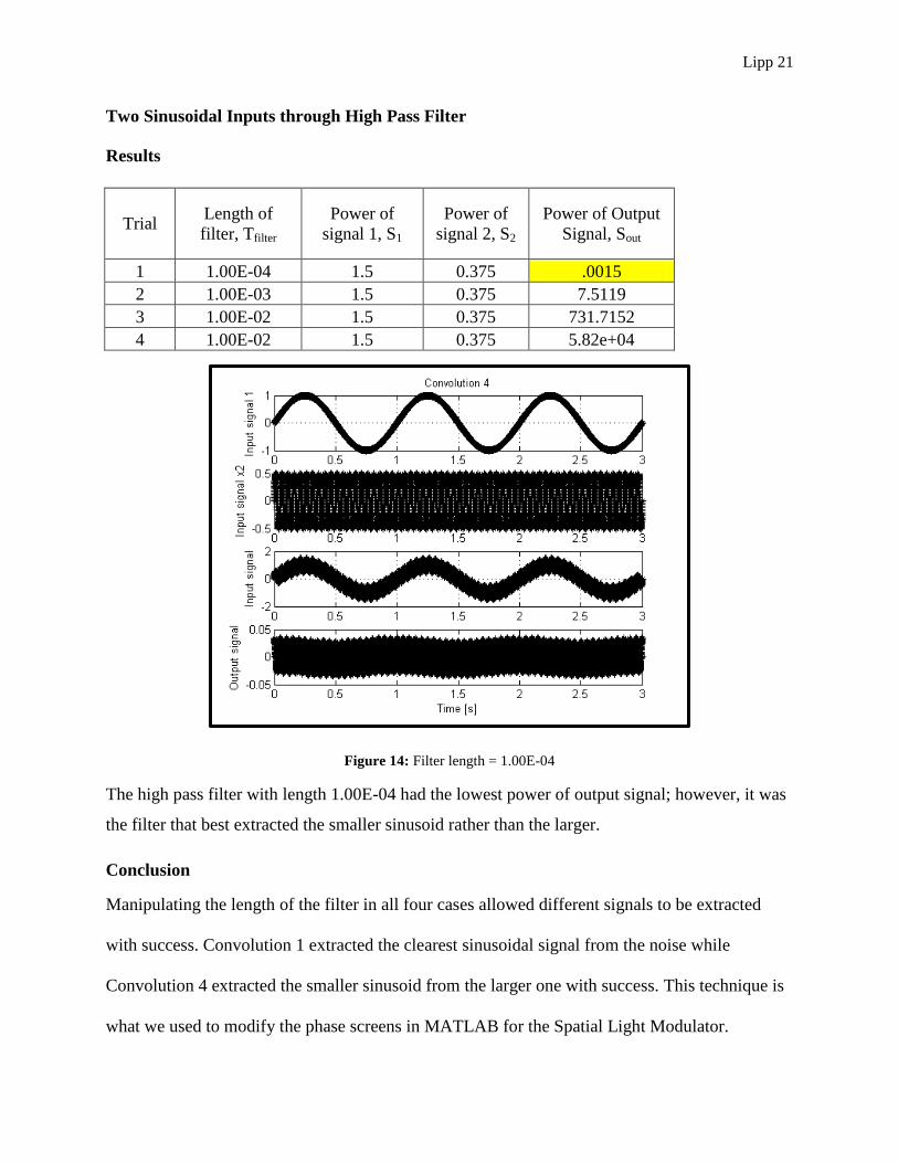
Two Sinusoidal Inputs through High Pass Filter

Results

Trial Length of

filter, Tfilter

Power of

signal 1, S1

Power of

signal 2, S2

Power of Output

Signal, Sout

1 1.00E-04 1.5 0.375 .0015

2 1.00E-03 1.5 0.375 7.5119

3 1.00E-02 1.5 0.375 731.7152

4 1.00E-02 1.5 0.375 5.82e+04


The high pass filter with length 1.00E-04 had the lowest power of output signal; however, it was

the filter that best extracted the smaller sinusoid rather than the larger.

Conclusion

Manipulating the length of the filter in all four cases allowed different signals to be extracted

with success. Convolution 1 extracted the clearest sinusoidal signal from the noise while

Convolution 4 extracted the smaller sinusoid from the larger one with success. This technique is

what we used to modify the phase screens in MATLAB for the Spatial Light Modulator.

Lipp 22

Research Summary

Research in developing lasers for use in communications and as a directed energy

weapon in the maritime environment is being conducted. However, because of the effects air

turbulence, optical turbulence, and temperature have on a beam, using lasers in these areas has

not yet been utilized to its full potential. Turbulence can result in increased scintillation which

causes fades at the target. By manipulating the phase of the beam using spatial light modulation,

a new beam can be created with a “flat top” profile rather than the typical Gaussian form. Voelz

and Fitzhenry have discussed a similar beam, formally known as a pseudo-partially coherent

beam (PPCB). This research propagates PPCBs through a hot air turbulence emulator capable of

simulating low to strong fluctuation conditions, recording the intensity and scintillation at the

target. The PPCBs can be created with different spatial coherence levels, which can be compared

to the standard Gaussian form, to determine their success in propagating through the turbulence.

In addition, this research explores the effects that cycling different phase screens has on the

success of propagating the PPCBs through turbulence. Theory predicts that by cycling PPCBs at

a rate faster than the atmosphere changes will result in decreased intensity fluctuations at the

target. The goal of this project is to minimize scintillation variations at the target after passing

the beam through high turbulence.

This past semester, we succeeded in setting up the turbulence emulator, constructed by

Assistant Professor Nelson for his dissertation. Also, we propagated laser beams through the

emulator using phase screens constructed using MATLAB and convolution theory. These phase

screens had different coherence levels, with black corresponding to perfect phase coherence.

Finally, we succeeded in running trials to obtain preliminary results on the PPCBs described by

Voelz and Fitzhenry.

Lipp 23

Equipment

- ThorLabs HNL020L 632.8 nm Helium Neon Laser

- BNS Spatial Light Modulator (SLM) – XY Series

- ThorLabs DCU224M - CCD Camera

- 11 Amp Variable Temperature Heat Gun

- Thorlabs BEDS-10-A Expander

- Thermaltake Fans

- Omega 12 Channel Temperature Recorder RDXL 12SD

Emulator Setup

An emulator is used to mimic some of the effects of high turbulence found by

propagating a beam over a long range in just a laboratory setting. It provides quick and easy

control over turbulence strength, is statistically repeatable, provides a random optical turbulence

as compared with a static phase screen that is rotated and has a repeating phase pattern, and is

modular and extendable. The setup includes four heat guns providing thermal flow of 200 °F

which are opposed by four fans providing ambient air counter flow. The heat from the guns is

dispersed by three diffuser screens set in front of the heat guns. There are temperature probes

spaced evenly throughout taking temperature readings every second. Previous analysis of these

temperature changes categorized the turbulence as approximately Kolmogorov along the beam

propagation axis with an average Cn2 value of 3.81E-11. Figures 15 and 16 below illustrate the

setup.

Lipp 24

Figure 15: Laser’s path through emulator into DC camera

Figure 16: Side view of emulator displaying heat guns and Temperature Recorder

Lipp 25

Laser, Expander, and SLM Setup

The laser is first propagated through an expander and then reflected off of the SLM, as

shown in Figure 17.

SLM Screens

Using MATLAB and convolution, the screens for the SLM can be produced. The Multi-

Gaussian Schell Model is used to make the screens, using different levels of coherence. Some

sample screens are shown below.

Laser Expander SLM Figure 9

Figure 17: Laser, Expander and SLM setup

Black

(perfectly coherent) SLM Screen 2

(strong diffuser)

SLM Screen 8

(weaker diffuser)

Lipp 26

Process

- Start camera and SLM

- Warm up heat guns and fans

- Begin temperature collection

- Begin cycling

- Begin camera recording

- Convert video to jpeg images

- Analyze jpegs in MATLAB to find scintillation index and intensity

Results

Below is a graph of scintillation index versus coherence. When propagating beams, scintillation

should be minimized. The data indicates that all but one of the partially coherent beams had a

lower scintillation index than that of black.

0

0.02

0.04

0.06

0.08

0.1

0.12

1 2 4 8

Scin

tillation Index

Correlation Width

Scintillation with Turbulence

Cycling

No Cycling

Lipp 27

Conclusion

This experiment’s goal was to examine the effects of pseudo-partially spatially coherent beams

through turbulence. Ideally, the scintillation index would be minimized. However, initial results

indicate that the scintillation was lower for all of the partially coherent beams. In addition, the

pseudo-partially coherent beams had higher scintillation than the partially coherent beams

through turbulence. This may be due to the fact that the SLM affected the pseudo-partially

coherent beams when changing phase screens so rapidly. Further study will allow us to explore

how to reduce scintillation using pseudo-partially coherent beams while maintaining intensity.

Lipp 28

References

Pedrotti, Pedrotti, and Pedrotti. Introduction to Optics, Third Edition. Pearson, 2007.

S.O. Kasap. Optoelectronics and Photonics: Principles and Practices, Second Edition. Pearson,

2007.

Voelz, David and Kevin Fitzhenry. “Pseudo-partially Coherent Beam for Free-space Laser

Communication.”

Qian, Xianmei, Wenyue Zhu and Ruizhong Rao. “Numerical Investigation on Propagation

Effects of Pseudo-partially Coherent Gaussian Schell-model Beam in Atmospheric

Turbulence.” Optical Society of America. 26 February 2009.

C. Nelson, S. Avramoz-Zamurovic, O. Korotkova, R. Malek-Madani, R. Sova, and F. Davidson.

“Measurements of partially spatially coherent laser beam intensity fluctuations propagating

through a hot-air turbulence emulator and comparison with both terrestrial and maritime

environments.”

C. Nelson. “Experiments in Optimization of Free Space Optical Communication Links for

Applications in a Maritime Environment,” dissertation from John Hopkins University, 2013.

Lipp 29

Appendix

Convolution 1: Sinusoidal Input with Noise through Low Pass Filter

Input signals

clear

dt = 5*10^-6;

period=1/1000; % Since the signal frequency is 1 kHz

Tx = 3*period;

t=0:dt:Tx; % Let us show 3 periods

x = 2*sin(2000*pi*t);% Input signal

n = 5*randn(size(x));% Generates random noise

S = sum((x.^2)*dt);% Power of the input

N = sum((n.^2)*dt);% Power of the noise

Ratio = S/N;% Ratio between power of input and noise

y = x + n;% Input plus noise

Building the filter

for i=1:4;

tfilter = i*.25*period; % Filter lasts .5 signal periods. Modify for best results

tfup=0:dt:tfilter;

F=ones(size(tfup));% Builds filter

c=conv(y,F);% Convolution of filter and input signal with noise

tconv=0:dt:(length(c)-1)*dt;

Sout(i) = sum((c.^2)*dt);% Power of the output signal

Ratio_out = Sout/N;

Plotting results

figure(1)

subplot(311);plot(t,x,'k*');grid;

title('Convolution 1');

ylabel('Input signal');

subplot(312);plot(t,y,'k*');grid;

ylabel('Input with noise');

subplot(313);plot(tconv,c,'k*');grid;

ylabel('Output signal')

xlabel('Time [s]')

end

Lipp 30

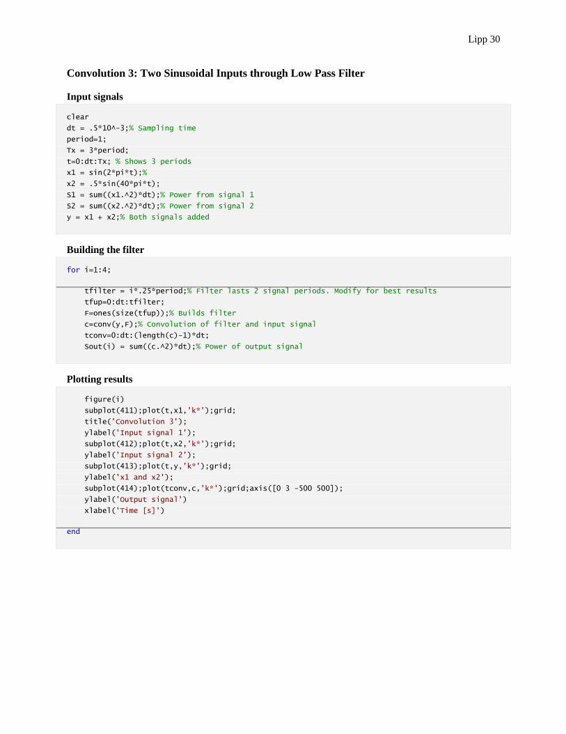
Convolution 3: Two Sinusoidal Inputs through Low Pass Filter

Input signals

clear

dt = .5*10^-3;% Sampling time

period=1;

Tx = 3*period;

t=0:dt:Tx; % Shows 3 periods

x1 = sin(2*pi*t);%

x2 = .5*sin(40*pi*t);

S1 = sum((x1.^2)*dt);% Power from signal 1


y = x1 + x2;% Both signals added

Building the filter

for i=1:4;

tfilter = i*.25*period;% Filter lasts 2 signal periods. Modify for best results

tfup=0:dt:tfilter;

F=ones(size(tfup));% Builds filter

c=conv(y,F);% Convolution of filter and input signal


Sout(i) = sum((c.^2)*dt);% Power of output signal

Plotting results

figure(i)

subplot(411);plot(t,x1,'k*');grid;


ylabel('Input signal 1');




ylabel('x1 and x2');

subplot(414);plot(tconv,c,'k*');grid;axis([0 3 -500 500]);


xlabel('Time [s]')

end

Lipp 31

Convolution 2: Sinusoidal Input with Noise through High Pass Filter

Input signals

clear

dt = 5*10^-6;

period=1/1000; % Since the signal frequency is 1 kHz

Tx = 3*period;

t=0:dt:Tx; % Let us show 3 periods

x = 2*sin(2000*pi*t);% Input signal

n = 5*randn(size(x));% Generates random noise

S = sum((x.^2)*dt);% Power of the input

N = sum((n.^2)*dt);% Power of the noise

Ratio = S/N;% Ratio between power of input and noise

y = x + n;% Input plus noise

Building the filter

for i=1:4;

T2 = i*.25*period;

T3 = i*.25*period;% Filter lasts 2 periods. Modify for best results

tup=0:dt:T2;% Length of time filter equals 1

tdown=T2+dt:dt:T3+dt;% Length of time filter equals -1

FilterHP = [ ones(size(tup)) -ones(size(tdown))];% Builds filter

c=conv(y,FilterHP);% Convolution of filter with input noise


Sout(i) = sum((c.^2)*dt);% Power of output signal

Ratio_out = Sout/N;

Plotting results

figure(i)

subplot(311);plot(t,x,'k*');grid;




ylabel('Input with noise');

subplot(313);plot(tconv,c,'k*');grid;


xlabel('Time [s]')

end

Lipp 32

Convolution 4: Two Sinusoidal Inputs through High Pass Filter

Input signals

clear

dt = .5*10^-3;% Sampling time

period=1;

Tx = 3*period;

t=0:dt:Tx; % Shows 3 periods

x1 = sin(2*pi*t);%

x2 = .5*sin(40*pi*t);



y = x1 + x2;% Both signals added

Building the filter

T2 = .0001*period;

T3 = .0001*period;% Modify for best results

tup=0:dt:T2;% Length of time filter equals 1

tdown=T2+dt:dt:T3+dt;% Length of time filter equals -1

FilterHP = [ ones(size(tup)) -ones(size(tdown))];% Builds filter

c=conv(y,FilterHP);% Convolution of filter with input noise


Sout = sum((c.^2)*dt);% Power of output signal

Plotting results

figure(1)





ylabel('Input signal x2');



subplot(414);plot(tconv,c,'k*');grid;axis([0 3 -.05 .05]);


xlabel('Time [s]')

Documents

Report - USNA stuff/Report... · Report SM495 Meredith Lipp ... Stimulated Emission, Photon Amplification, and Lasers ... by S. O. Kasap, New York, 2013. Lipp 12