Report on Socio-Economic Disparities in

Madhya Pradesh

Working Paper I

Poverty Monitoring and Policy Support Unit State Planning Commission

C- wing, First Floor, Vindhyachal Bhawan, Bhopal, Madhya Pradesh

Forward Poverty Monitoring and Policy Support Unit is bringing out its first working paper entitled “Socio

Economic Disparities in Madhya Pradesh” based on data of State Sample of 61st

round of NSS (July

2004-June 2005). This is first time in the state that an attempt has been made to analyze the data of

State sample of NSS of any round.

On the basis of analysis of data, present report covers various aspects such as Distribution of

households and population by socio-economic classes, Distribution of households by type of

households, Distribution of households by type of land owned, Distribution of households by social

groups and type of fuel used, Distributions of households by primary source of energy for cooking or

lighting, Reach of various programmes, Holding of various type of ration cards, Distribution of

households by MPCE classes, Average monthly per capita expenditure and inequality among different

socio groups in consumption etc, are presented for the State of Madhya Pradesh. This paper reveals

the disparities among various socio economic categories of households. Gini Coefficient which is the

indicator of inequality for different socio – economic categories has been presented in the paper. In

addition, Average Poverty Gap, Poverty Gap Index and Squared Poverty Gap Index for different MPCE

classes by Socio-Groups have worked out and presented.

I hope that this paper may serve as input to policy makers for developing policies for alleviating

poverty and its implementation in more effective way.

I hope that in future PMPSU will come up with more working papers on the issues which concern

most to the public of state.

I wish, PMPSU will work with its sincerity and devotion for the progress of state and achieve its aim

for which it has been set up.

Mangesh Tyagi

Advisor SPC,M.P.

& Nodal Officer PMPSU CELL

Executive Summary The purpose of analysis of State Sample is to provide insight on some of issues to the policy makers,

planners and implementers, which require to be attended to reduce disparity and inequalities.

This is first time in the state that State Sample of any NSS round has been analysed. It is first initiative

of PMPSUS. More detailed work has been planned for year to come.

The major findings of present study are:

Distribution of households and Population by socio-economic classification:

Scheduled tribes households’ accounts for 19.94 percent of total household and around 17.77

percent of households belonging to scheduled castes are there in the state. Other Backward

Classes accounted for 38.91 percent of households are highest in state. Other households are

slightly less than one fourth of total households.

Type of Households:

In urban area 44.19 % household earning income from self-employment, 32.61 % from

salaries/regular wages, 17.18 % earn their livelihood by working as casual labour and 6.02 %

from other activities. Among self employed households the representation is more of OBC

and others as compare to their population while in case of salary earning households the

representation of ST and others is more. In case of SC and OBC their representation is less by

4.5 and 5 percentage points than their proportion in population respectively.

In Rural areas, 76.31 % of households earning their livelihood from agricultural activities,

which includes 29.03 % households who are working as agricultural labourers in rural area of

the state. 11.73 % of total households come under Self Employed-non agriculture category.

Among self employed in agriculture households the presentation is more of OBC and others

as compare to their population. It is also true for self employed in non agriculture.

Use of Primary Source of Energy:

Cooking:

It is observed that in urban areas of the state, during 2004-05, 58.1 % of households were

using LPG as fuel, 37.4 % using firewood, 2.1 % using kerosene and 2.0 % using dung cake

for cooking. The LPG users accounts for 42.6 % among ST households, 28.3 % among SC

households, 55.2 % among OBC households and 72.8 % among other households. Majority of

households of Scheduled tribes and Castes, firewood and chips are major source of fuel for

cooking. Among total LPG users, 3.4 % belonged to ST category, 7.4 % to SC, 35.7 % to

OBC and others accounted for 53.6 percent showing disproportionate distribution of better

fuel to their respective population.

In rural areas, penetration of use of LPG for cooking is found to be low at 3.95 percent. Fuel

wood is widely used for cooking by 93.43 % of rural households though use of dung cake is

limited to 2.51 percent of households. The reason for use of firewood by large proportion of

all social groups is availability of fire wood from nearby forests. Among firewood user

households 65% are accounted by ST and OBC households. In case of LPG users 79.4 % are

others and OBC households. Majority of dung cake users’ households belong to OBC and

others category of households.

Lighting:

Electricity is the major source for lighting in both urban and rural area of the state. 88.48 % of

households are using electricity for lighting in the state. In urban area user households

accounts for 97 % of total households while for rural area it is 83.4 percent. The access to

electricity is almost equitable to all socio groups irrespective of their place of residence.

Marginal distortion in case ST and SC is observed in both urban and rural area.

Access to Various Programmes

State sample of 61st Round of NSSO reveals that Food for Work programme could reach to1.0

% of households, Annapoorna 0.5 % households, ICDS 5.7 % and Midday Meal could reach

30.37 percent of households in the state. Midday Meal could reach 35 percent of households

in rural area while in urban it was able to reach 13.5 % of households. It is also observed that

programme could reach ST, SC and OBC relatively more than state average reach.

Ration Card Holding:

To provide subsidized food grain to the subjects belonging to poor section of the society, Food

and Civil Supply Department had issued different type of ration cards namely, Antodaya card,

BPL card and other cards.

In state around 73 % of urban households, 83 % of rural households and overall 80% of the

households own ration card. Among social groups, highest proportion of SC households (85.4

%) was holding ration cards in the state. It is true for both urban and rural areas. In urban

areas, it is followed by Others (73.5 %), OBC (71 %) and lowest proportion of household

owning ration card was ST with 68.3 %. In case of rural, after SC households second highest

proportion is observed for OBC household (83.7 %) followed by ST with 81.2 % and 79.9 %

of other households owned ration card.

The proportion of different types of ration card among card holders revealed that Antodaya

Card meant for the poorest among poor, accounts for merely 1.3 percent of the ration card

holders and BPL card holders accounted for 25.2 percent while remaining households owned

other cards in the state.

Expenditure Pattern and Inequality

Monthly Per Capita Expenditure:

Instead of 12 MPCE classes adopted by NSSO, for the present study four MPCE classes have

been formed by clubbing, in urban areas monthly per capita expenditure classes adopted are

less than Rs. 485, Rs. 485-930 and more than Rs. 930 which work out to less than Rs.16.16,

24.33 and more than Rs.31 per capita par day. For rural area these classes are less than Rs.

455, Rs. 455-890 and more than Rs. 890 which work out to less than Rs.15.16, 22.43 and

more than Rs.30 per capita par day.

Urban Area:

Analysis reveals that in urban areas there were 24.5 percent of total households with MPCE

less than Rs. 485. 28.1 % of households having MPCE more than Rs. 930 while remaining

47.4 % of households having MPCE in range of Rs. 485 to Rs. 930. Among SC households,

the proportion of households with MPCE more than Rs.930 is lowest at 12.1 % followed by

ST with 13.8 % and OBC with 21.1 %. It shows that majority of SC households (87.9 %) are

incurring consumer expenditure less than Rs. 24 per capita per day on an average basis. The

proportion of similar households in ST and OBC categories are 86.2 % and 78.9 %

respectively. Among other households such households constitute for 58.5 % of total

households.

Results reveal that around three fourth of total households with MPCE less than Rs. 485

belong to OBC and ST categories. The distribution of households in MPCE class of Rs. 485

to Rs. 930 shows that to large extent is same as their proportion in total population. Highest

category of MPCE (i.e. more than Rs. 930) is dominated by “Other Households”. It shows

that significantly good proportion of SC, OBC and ST are relatively not better off than other

households.

ST households belonging to MPCE category of Rs. 485-930 are spending more than (on an

average basis) households of other socio groups and all households. OBC households are

spending more as compare to (on an average basis) other socio groups in lower and higher

MPCE classes. Households of Lower MPCE class of less than Rs. 485 are spending less than

one fourth of their respective counter parts in higher MPCE class except in case of SC

households who are spending 29 percent and ST households who are spending 21 percent of

their counterparts in higher MPCE class. ST households of lower MPCE class are spending

less than half than their counter parts in next higher MPCE class of Rs. 485 to Rs. 930.

Rural Areas:

There were 44.5 percent of total households with MPCE less than Rs. 455. Merely 7.9 % of

households having MPCE more than Rs. 890 while remaining 47.6 % of households having

MPCE in range of Rs. 455 to Rs. 890. Among other households, the proportion of

households with MPCE more than Rs.890 is highest at 17.1 % followed by OBC with 9.3 %

and ST with 3.2 %. It also reveals that majority of SC households (97.8 %) are incurring

consumer expenditure less than Rs. 22.43 per capita per day on an average basis.

ST and SC households are spending less than average spending of all households irrespective

of MPCE class. OBC and Other households are spending more as compare to all households

put together. Households of Lower MPCE class of less than Rs. 455 are spending around one

third of their counter parts in higher MPCE class and 60 % of those in middle MPCE class of

Rs. 455 to Rs. 890 irrespective of social class. This table also reveals that in rural areas among

SC and ST households intake is below the state average.

The proportion of households for different consumption levels have similar pattern or not. To

analyse this aspect, in urban area the consumption level assumed are below Rs300, Rs. 350,

Rs. 400, Rs450, Rs. 500, Rs. 550 and Rs. 600 while in rural areas first four level have been

considered. This analysis will reveal that an increment in consumption level by Rs.50 what

proportion of total households get included. In other word, these households can be treated as

target group which can be moved from one category of consumption class to another by some

interventions comparatively of smaller magnitude than moving all the households belonging

to lower MPCE class for which interventions of larger magnitudes are required. Details are in

main paper.

Average Poverty Gap, Inequality among different Socio Groups and Poverty Gap Index for

different MPCE classes by Socio-Groups have worked out and presented in main paper.

Introduction

The NSSO conducts regular consumer expenditure surveys as part of its “rounds”, each round

normally of a year’s duration and covering more than one subject of study. The surveys are conducted

through household interviews, using a random sample of households covering practically the entire

geographical area of the country. Each State also conducts the same survey with equal sample known

as STATE SAMPLE.

This is first time, an attempt is made to analyses the State Sample of the data collected in any NSS

round in the state. The present report is based State sample for which data was collected through the

61st

round of NSS (July 2004-June 2005). On the basis of analysis of data, present report covers

various aspects such as Distribution of households and population by socio-economic classes,

Distribution of households by type of households, Distribution of households by type of land owned,

Distribution of households by social groups and type of fuel used, Distributions of households by

primary source of energy for cooking or lighting, Reach of various programmes, Holding of various

type of ration cards, distribution of households by MPCE classes, average monthly per capita

expenditure and inequality among different socio groups in consumption etc, are presented for the

State of Madhya Pradesh. All the results are presented separately for rural and urban households.

Some details of the survey:

Madhya Pradesh participated in the survey: a “State sample” was surveyed by State Government

officials of National Sample Survey Division of Directorate of Economic and Statistics. For rural

Madhya Pradesh, 384 villages formed the State sample for this round. Of these, 383 villages were

ultimately surveyed. In the urban sector, the allocation for the state sample was 208 blocks, of which

206 were surveyed. This report is based on the estimates obtained from the State sample alone.

Table 1 shows the number of villages and urban blocks allotted for survey and the numbers actually

surveyed, and the number of households in which the consumer expenditure schedule, “Schedule 1.0”,

was canvassed.

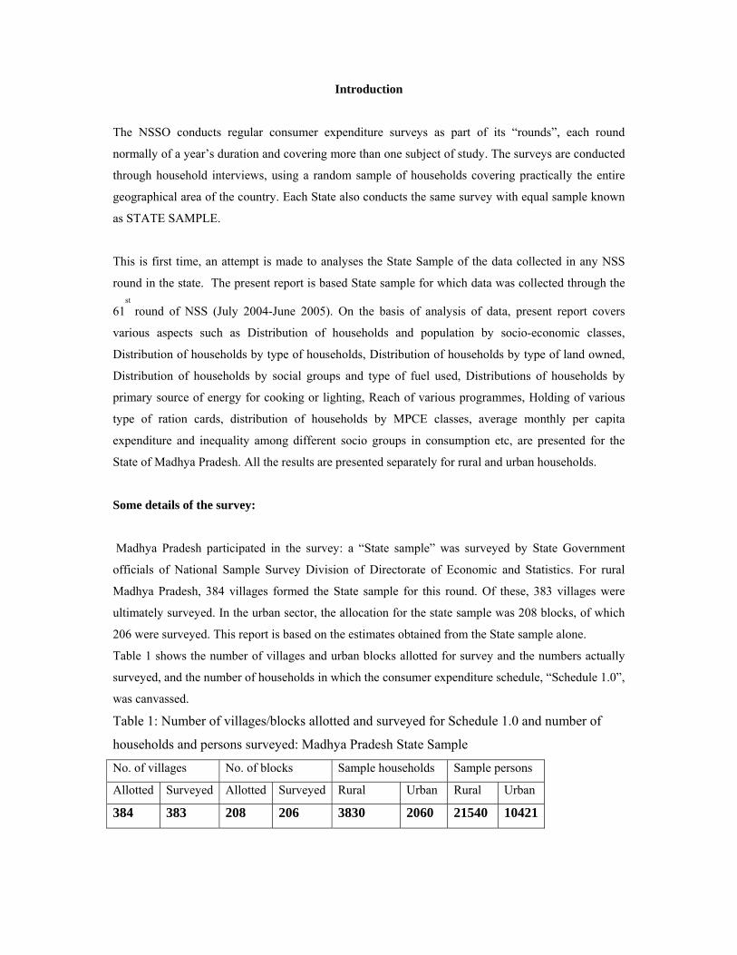
Table 1: Number of villages/blocks allotted and surveyed for Schedule 1.0 and number of

households and persons surveyed: Madhya Pradesh State Sample

No. of villages No. of blocks Sample households Sample persons Allotted Surveyed Allotted Surveyed Rural Urban Rural Urban

384 383 208 206 3830 2060 21540 10421

Concepts and Definitions

Household:

A group of persons normally living together and taking food from a common kitchen constitutes a

household. The word "normally" means that temporary visitors are excluded but temporary stay-

aways are included. Thus, a son or daughter residing in a hostel for studies is excluded from the

household of his/her parents, but a resident employee or resident domestic servant or paying guest

(but not just a tenant in the house) is included in the employer/host's household. "Living together" is

usually given more importance than "sharing food from a common kitchen" in drawing the boundaries

of a household in case the two criteria are in conflict; however, in the special case of a person taking

food with his family but sleeping elsewhere (say, in a shop or a different house) due to space shortage,

the household formed by such a person's family members is taken to include the person also. Each

inmate of a mess, hotel, boarding and lodging house, hostel, etc. is considered as a single-member

household except that a family living in a hotel (say) is considered as one household only; the same

applies to residential staff of such establishments.

Household size:

The size of a household is the total number of persons in the household.

Household consumer expenditure:

The expenditure incurred by a household on domestic consumption during the reference period is the

household's consumer expenditure. Household consumer expenditure is the total of the monetary

values of consumption of various groups of items, namely (i) food, pan (betel leaves), tobacco,

intoxicants and fuel & light, (ii) clothing and footwear and (iii) miscellaneous goods and services and

durable articles.

For groups (i) and (ii), the total value of consumption is derived by aggregating the monetary value of

goods actually consumed during the reference period. An item of clothing and footwear would be

considered to have been consumed if it is brought into maiden or first use during the reference period.

The consumption may be out of (a) purchases made in cash or credit during the reference period or

earlier; (b) home-grown stock; (c) receipts in exchange of goods and services; (d) any other receipt

like gift, charity, borrowing and (e) free collection. Home produce is evaluated at the ex farm or ex

factory rate. For evaluating the consumption of the items of group (iii), i.e., items categorised as

miscellaneous goods and services and durable articles, a different approach is followed. In this case,

the expenditure made during the reference period for the purchase or acquisition of goods and services

is considered as consumption.

It is pertinent to mention here that the consumer expenditure of a household on food items relates to

the actual consumption by the members of the household and also by the guests during ceremonies or

otherwise. To avoid double counting, transfer payments like charity, loan advance, etc. made by the

household are not considered as consumption for items of groups (i) and (ii), since transfer receipts of

these items have been taken into account. However, the item "cooked meals" is an exception to the

rule. Meals prepared in the household kitchen and provided to the employees and/or others would

automatically get included in domestic consumption of employer (payer) household. There is a

practical difficulty of estimating the quantities and values of individual items used for preparing the

meals served to employees or others. Thus, to avoid double counting, cooked meals received as

perquisites from employer household or as gift or charity are not recorded in the recipient household.

As a general principle, cooked meals purchased from the market for consumption of the members and

for guests and employees will also be recorded in the purchaser household.

This procedure of recording cooked meals served to others in the expenditure of the serving

households only leads to bias-free estimates of average per capita consumption as well as total

consumer expenditure. However, donors of free cooked meals are likely to be concentrated at the

upper end of the per capita expenditure range and the corresponding proportion of recipients at the

lower end of the same scale. Consequently, the derived nutrition intakes may get inflated for the rich

(net donors) and understated for the poor (net recipients). This point has to be kept in mind while

interpreting the NSS consumer expenditure data for any studies relating to the nutritional status of

households.

Value of consumption:

Consumption out of purchase is evaluated at the purchase price. Consumption out of home produce is

evaluated at ex farm or ex factory rate. Value of consumption out of gifts, loans, free collections, and

goods received in exchange of goods and services is imputed at the rate of average local retail prices

prevailing during the reference period.

Monthly per capita consumer expenditure (MPCE):

For a household, this is the total consumer expenditure over all items divided by its size and expressed

on a per month (30 days) basis. A person’s MPCE is understood as that of the household to which he

or she belongs.

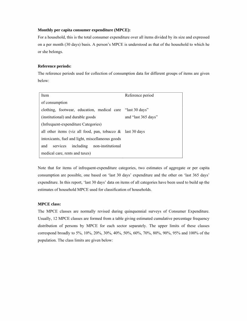
Reference periods:

The reference periods used for collection of consumption data for different groups of items are given

below:

Item

of consumption

Reference period

clothing, footwear, education, medical care

(institutional) and durable goods

(Infrequent-expenditure Categories)

“last 30 days”

and “last 365 days”

all other items (viz all food, pan, tobacco &

intoxicants, fuel and light, miscellaneous goods

and services including non-institutional

medical care, rents and taxes)

last 30 days

Note that for items of infrequent-expenditure categories, two estimates of aggregate or per capita

consumption are possible, one based on ‘last 30 days’ expenditure and the other on ‘last 365 days’

expenditure. In this report, ‘last 30 days’ data on items of all categories have been used to build up the

estimates of household MPCE used for classification of households.

MPCE class:

The MPCE classes are normally revised during quinquennial surveys of Consumer Expenditure.

Usually, 12 MPCE classes are formed from a table giving estimated cumulative percentage frequency

distribution of persons by MPCE for each sector separately. The upper limits of these classes

correspond broadly to 5%, 10%, 20%, 30%, 40%, 50%, 60%, 70%, 80%, 90%, 95% and 100% of the

population. The class limits are given below:

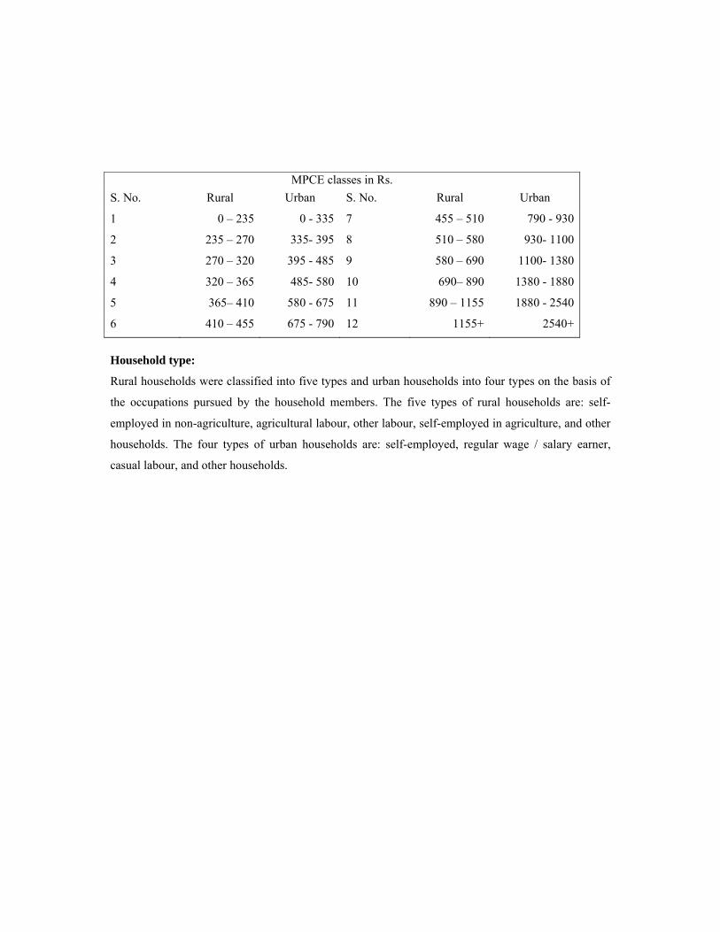
Household type:

Rural households were classified into five types and urban households into four types on the basis of

the occupations pursued by the household members. The five types of rural households are: self-

employed in non-agriculture, agricultural labour, other labour, self-employed in agriculture, and other

households. The four types of urban households are: self-employed, regular wage / salary earner,

casual labour, and other households.

MPCE classes in Rs. S. No. Rural Urban S. No. Rural Urban

1 0 – 235 0 - 335 7 455 – 510 790 - 930

2 235 – 270 335- 395 8 510 – 580 930- 1100

3 270 – 320 395 - 485 9 580 – 690 1100- 1380

4 320 – 365 485- 580 10 690– 890 1380 - 1880

5 365– 410 580 - 675 11 890 – 1155 1880 - 2540

6 410 – 455 675 - 790 12 1155+ 2540+

The “Type” of a household was determined as follows:

Rural:

A household was classified as “agricultural labour”, if its income during the last 365 days preceding

the date of survey from that source was 50% or more of its total income. The same criterion was

followed to classify a household as “self-employed in agriculture”. A household was classified as

“self-employed in non-agriculture” if its income from that source was greater than that from rural

labour as well as that from all other gainful sources put together. If a household was not one of these

three types but its income from total rural labour was greater than that from all self-employment and

from other gainful sources, it was classified as “other labour”. The remaining households were

classified as “other households”.

Urban:

A household was classified as “self-employed”, “regular wage or salary earning”, or “casual labour”,

according to the major sources of its income from “gainful employment” during the 365 days

preceding the date of survey. A household not having any income from gainful employment was

classified under “others”.

Social Group: There are in all four social groups, namely, scheduled caste (SC), scheduled tribe (ST),

other backward class (OBC) and Others. Those who did not come under any one of the first three

social groups were assigned to ‘Others’ meant to cover all other categories. In case different members

of a household belonged to different social groups, the group to which the head of the household

belonged was considered as the ‘social group’ of the household.

Source of energy for cooking:

The source of energy used by a household during the last 30 days preceding the date of survey has

been ascertained and collected in the survey. The type of sources are as follow coke/ coal, firewood

and chips, LPG , gobar gas, dung cake, charcoal , kerosene, electricity and others.

If a household used more than one of the above sources then the one having major use has been

assigned to the household. The term used for this source is primary source of energy for cooking.

Source of energy for lighting:

Like source of energy for cooking, the source of energy for lighting used by households during the

last 30 days preceding the date of survey has been ascertained and collected in the survey. The

different types of sources are kerosene, other oil, gas, candle, electricity and others. If a household

used more than one of the above sources for lighting then the one having major use has been assigned

to the household. The term used for this source is primary source of energy for lighting.

The report gives information on the primary source of energy separately for cooking and lighting used

by the households. It ignores the sources other than the primary sources used by the households.

In addition, data has been collected from the households regarding holding of various type of ration

cards and whether households has been benefited by programmes like Mid Day Meal, ICDS etc.

Sample Design A stratified multi-stage design has been adopted for the 61st round survey. The first stage

units (FSU) are the 2001 census villages in the rural sector and Urban Frame Survey (UFS)

blocks in the urban sector. The ultimate stage units (USU) are households in both the sectors.

In the case of large villages/blocks requiring hamlet-group (hg)/sub-block (sb) formation, one

intermediate stage is the selection of two hgs/sbs from each FSU. The sample of villages and

urban blocks for state sample has been selected by NSSO. The estimation procedure as

provided by NSSO is used. Details of sample design and estimation procedure is given in

annexure, which is being reproduced from NSSO Report Number 508.

General Profile of Households and Disparity in Madhya Pradesh

Socio- economic Classification:

Scheduled tribes households’ accounts for 19.94 percent of total household and around 17.77 percent

of households belonging to scheduled castes are there in the state. Other Backward Classes accounted

for 38.91 percent of households are highest in state. Other households (not belonging to scheduled

tribe, scheduled caste and OBC categories) are slightly less than one fourth of total households.

The concentration of scheduled tribe and scheduled caste is more in rural area while OBC are almost

equally concentrated in rural and urban areas of the state. Others are more in urban areas in percentage

term. Distribution of households and population by socio-economic classification is presented in

figure 1 and Table 1.

Distribution of households and Population by socio-economic classification

4.59

24.51

19.94

4.26

24.22

19.93

15.118.57 17.17

15.3317.95 17.38

37.5339.33 38.91

36.8239.19 38.67

42.78

17.59

23.37

43.59

18.64

24.12

05

101520253035404550

Urban Rural Total Urban Rural Total

Households (%) Population (%)

Perc

enta

ge D

istri

butio

n

ST SC OBC Others

Table 1: Distribution of households and Population by socio-economic classification

Households (%) Population (%) Socio-economic Classification

Urban Rural Total Urban Rural Total

ST 4.59 24.51 19.94 4.26 24.22 19.93 SC 15.10 18.57 17.17 15.33 17.95 17.38 OBC 37.53 39.33 38.91 36.82 39.19 38.67 Others 42.78 17.59 23.37 43.59 18.64 24.12 All 100.00 100.00 100.00 100.00 100.00 100.00

Type of Households:

The households have been classified based on type of activity undertaken by head of household for

earning such as self-employed, regular wage/salary earning, casual labour and others in urban area

while in rural area the classification is slightly different, the classification adopted in rural area is self-

employed-non agriculture, agriculture labour, other labour, self-employed in agriculture and others.

Survey results revealed that in urban area 44.19 % household earning income from self-employment,

32.61 % from salaries/regular wages, 17.18 % earn their livelihood by working as casual labour and

6.02 % from other activities.

Figure 2:

Distribution of Households by Type of Livelihood: Urban

44.19

32.61

17.186.02

Self Employed Salary Earner Casual Labour Others

Table 2: Distribution of households by Type of Households: Urban (in %)

Type of Households Urban Self Employed 44.19 Salary Earner 32.61 Casual Labour 17.18 Others 6.02 All 100.00

It is observed that among self employed households the representation is more of OBC and others as

compare to their population while in case of salary earning households the representation of ST and

others is more. In case of SC and OBC their representation is less by 4.5 and 5 percentage points than

their proportion in population respectively.

Figure:

Distribution of households by Type of livelihood and Social Group: Urban

1.25.3

8.813.6

4.6

14.310.6

27

11.715.1

40.2

32.5

42.4

31.1

37.5

44.3

51.6

21.8

43.6 42.8

0

10

20

30

40

50

60

Self employed Salary earning Casual labour Others Total

Per

cent

age

ST SC OBC Others

Table -3: Distribution of households by Type of Household and Social Group: Urban (in %)

Type of Households Social Group

Self employed Salary earning

Casual labour Others Total

ST 1.2 5.3 8.8 13.6 4.6SC 14.3 10.6 27.0 11.7 15.1OBC 40.2 32.5 42.4 31.1 37.5Others 44.3 51.6 21.8 43.6 42.8Total 100.0 100.0 100.0 100.0 100.0

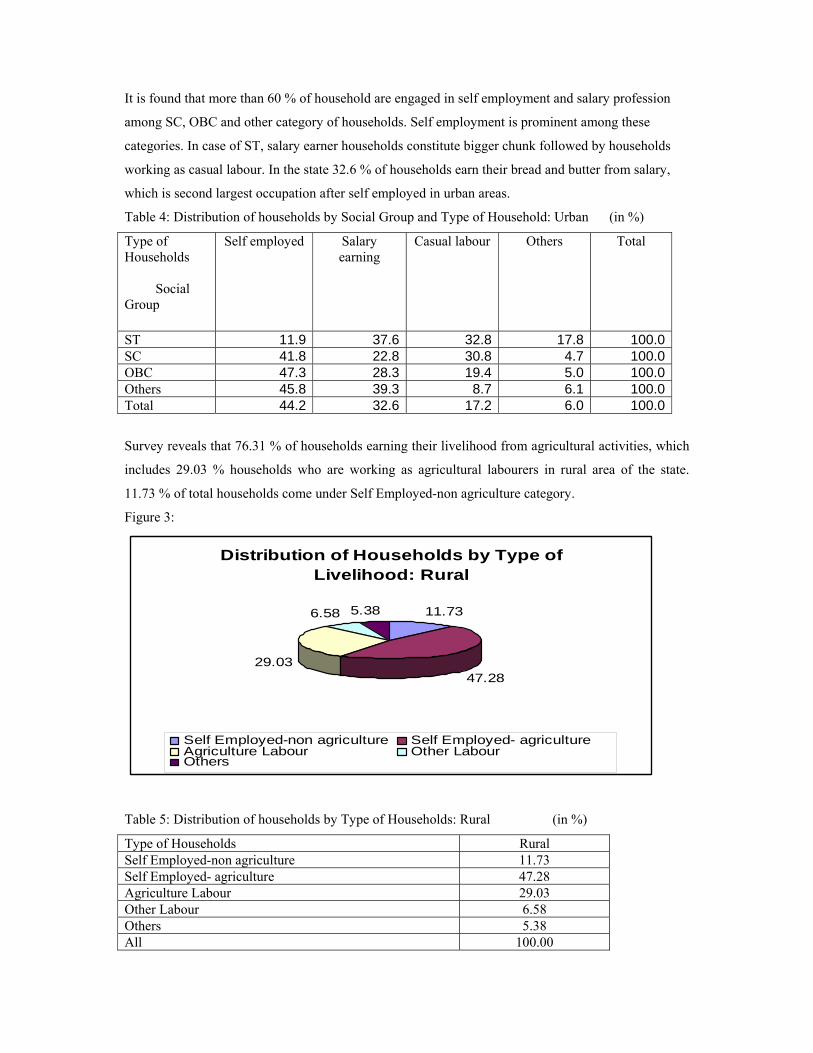
It is found that more than 60 % of household are engaged in self employment and salary profession

among SC, OBC and other category of households. Self employment is prominent among these

categories. In case of ST, salary earner households constitute bigger chunk followed by households

working as casual labour. In the state 32.6 % of households earn their bread and butter from salary,

which is second largest occupation after self employed in urban areas.

Table 4: Distribution of households by Social Group and Type of Household: Urban (in %)

Type of Households Social Group

Self employed Salary earning

Casual labour Others Total

ST 11.9 37.6 32.8 17.8 100.0SC 41.8 22.8 30.8 4.7 100.0OBC 47.3 28.3 19.4 5.0 100.0Others 45.8 39.3 8.7 6.1 100.0Total 44.2 32.6 17.2 6.0 100.0

Survey reveals that 76.31 % of households earning their livelihood from agricultural activities, which

includes 29.03 % households who are working as agricultural labourers in rural area of the state.

11.73 % of total households come under Self Employed-non agriculture category.

Figure 3:

Distribution of Households by Type of Livelihood: Rural

11.73

47.2829.03

6.58 5.38

Self Employed-non agriculture Self Employed- agricultureAgriculture Labour Other LabourOthers

Table 5: Distribution of households by Type of Households: Rural (in %)

Type of Households Rural Self Employed-non agriculture 11.73 Self Employed- agriculture 47.28 Agriculture Labour 29.03 Other Labour 6.58 Others 5.38 All 100.00

It is observed that among self employed in agriculture households the presentation is more of OBC

and others as compare to their population. It is also true for self employed in non agriculture.

Scheduled tribe and scheduled caste households’ forms major chunk of labour force engaged in

agriculture and other labour. A detail of participation by activity and social group is presented in

Table 6.

Table 6: Distribution of households by Type of Household and Social Group: Rural (in %)

Type of Households Social Group

Self Employed-

non agriculture

Self Employed- agriculture

Agriculture Labour

Other Labour

Others Total

ST 13.63 19.03 37.37 25.92 25.45 24.51 SC 17.29 9.44 28.28 43.04 19.20 18.57 OBC 49.68 47.30 27.23 23.78 30.92 39.33 Others 19.40 24.23 7.13 7.26 24.43 17.59 Total 100.00 100.00 100.00 100.00 100.00 100.00 Figure:

Distribution of households by Type of Livelihood and Social Group: Rural

13.619.0

37.4

25.9 25.5 24.51

17.3

9.4

28.3

43.0

19.2 18.57

49.747.3

27.223.8

30.9

39.33

19.424.2

7.1 7.3

24.4

17.59

0.0

10.0

20.0

30.0

40.0

50.0

60.0

Self Employed-non agriculture

Self Employed-agriculture

AgricultureLabour

Other Labour Others Total

Per

cent

ST SC OBC Others

It is observed that 65 % and 57 % of household from others and OBC group are occupied as self

employed in agriculture. Around 44 % of ST and SC are working as agricultural labour in rural areas.

The majority of the households depend upon cultivation and agricultural labour. 80.93 % of ST

households, 76.98 % of OBC, 76.88 % of other households and 68.35 % of SC households are

engaged in cultivation and agricultural labour respectively. A relative higher proportion as compare

to over all, OBC and Others are engaged in self employed non agricultural activities. Details are

presented in Table 7.

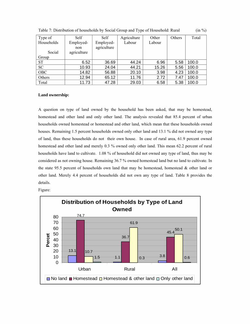
Table 7: Distribution of households by Social Group and Type of Household: Rural (in %)

Type of Households Social Group

Self Employed-

non agriculture

Self Employed- agriculture

Agriculture Labour

Other Labour

Others Total

ST 6.52 36.69 44.24 6.96 5.58 100.0 SC 10.93 24.04 44.21 15.26 5.56 100.0 OBC 14.82 56.88 20.10 3.98 4.23 100.0 Others 12.94 65.12 11.76 2.72 7.47 100.0 Total 11.73 47.28 29.03 6.58 5.38 100.0

Land ownership:

A question on type of land owned by the household has been asked, that may be homestead,

homestead and other land and only other land. The analysis revealed that 85.4 percent of urban

households owned homestead or homestead and other land, which mean that these households owned

houses. Remaining 1.5 percent households owned only other land and 13.1 % did not owned any type

of land, thus these households do not their own house. In case of rural area, 61.9 percent owned

homestead and other land and merely 0.3 % owned only other land. This mean 62.2 percent of rural

households have land to cultivate. 1.08 % of household did not owned any type of land, thus may be

considered as not owning house. Remaining 36.7 % owned homestead land but no land to cultivate. In

the state 95.5 percent of households own land that may be homestead, homestead & other land or

other land. Merely 4.4 percent of households did not own any type of land. Table 8 provides the

details.

Figure:

Distribution of Households by Type of Land Owned

13.1

1.1 3.8

74.7

36.745.4

10.7

61.9

50.1

1.5 0.3 0.60

1020304050607080

Urban Rural All

Per

cet

No land Homestead Homestead & other land Only other land

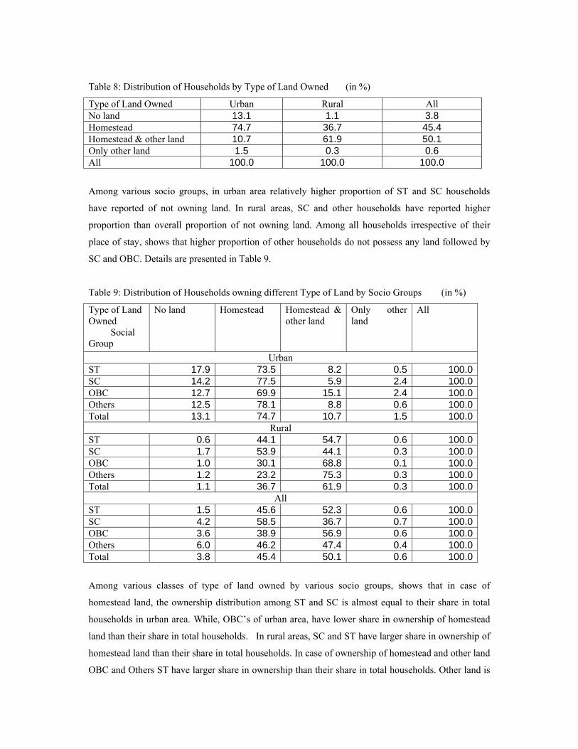
Table 8: Distribution of Households by Type of Land Owned (in %)

Type of Land Owned Urban Rural All No land 13.1 1.1 3.8 Homestead 74.7 36.7 45.4 Homestead & other land 10.7 61.9 50.1 Only other land 1.5 0.3 0.6 All 100.0 100.0 100.0

Among various socio groups, in urban area relatively higher proportion of ST and SC households

have reported of not owning land. In rural areas, SC and other households have reported higher

proportion than overall proportion of not owning land. Among all households irrespective of their

place of stay, shows that higher proportion of other households do not possess any land followed by

SC and OBC. Details are presented in Table 9.

Table 9: Distribution of Households owning different Type of Land by Socio Groups (in %)

Type of Land Owned Social Group

No land Homestead Homestead & other land

Only other land

All

Urban ST 17.9 73.5 8.2 0.5 100.0SC 14.2 77.5 5.9 2.4 100.0OBC 12.7 69.9 15.1 2.4 100.0Others 12.5 78.1 8.8 0.6 100.0Total 13.1 74.7 10.7 1.5 100.0

Rural ST 0.6 44.1 54.7 0.6 100.0SC 1.7 53.9 44.1 0.3 100.0OBC 1.0 30.1 68.8 0.1 100.0Others 1.2 23.2 75.3 0.3 100.0Total 1.1 36.7 61.9 0.3 100.0

All ST 1.5 45.6 52.3 0.6 100.0SC 4.2 58.5 36.7 0.7 100.0OBC 3.6 38.9 56.9 0.6 100.0Others 6.0 46.2 47.4 0.4 100.0Total 3.8 45.4 50.1 0.6 100.0

Among various classes of type of land owned by various socio groups, shows that in case of

homestead land, the ownership distribution among ST and SC is almost equal to their share in total

households in urban area. While, OBC’s of urban area, have lower share in ownership of homestead

land than their share in total households. In rural areas, SC and ST have larger share in ownership of

homestead land than their share in total households. In case of ownership of homestead and other land

OBC and Others ST have larger share in ownership than their share in total households. Other land is

reported to be owned by higher proportion of ST and others households as compare to their share in

population. Though, the area owned is not being considered in this exercise, disparity in ownership of

land (irrespective of area owned) among various socio groups has been found. Details are presented in

Table 10.

Table 10: Distribution of Households by Type of Land Owned (in %)

Type of Land Owned Social Group

No land Homestead Homestead & other land

Only other land

All

Urban ST 6.3 4.5 3.5 1.4 4.6SC 16.4 15.7 8.3 24.1 15.1OBC 36.5 35.1 52.8 58.5 37.5Others 40.9 44.7 35.3 16.0 42.8Total 100.0 100.0 100.0 100.0 100.0

Rural ST 12.6 29.4 21.7 50.7 24.5SC 29.8 27.2 13.2 18.4 18.6OBC 37.6 32.3 43.7 13.1 39.3Others 20.0 11.1 21.4 17.8 17.6Total 100.0 100.0 100.0 100.0 100.0

All ST 7.6 20.0 20.8 20.9 19.9SC 19.3 22.9 13.0 21.9 17.8OBC 36.7 33.3 44.1 40.5 38.9Others 36.3 23.8 22.1 16.7 23.4Total 100.0 100.0 100.0 100.0 100.0

Use of Primary Source of Energy

Cooking:

It is observed that in urban areas of the state, during 2004-05, 58.1 % of households were using LPG

as fuel, 37.4 % using firewood, 2.1 % using kerosene and 2.0 % using dung cake for cooking. The

LPG users accounts for 42.6 % among ST households, 28.3 % among SC households, 55.2 % among

OBC households and 72.8 % among other households. Majority of households of Scheduled tribes

and Castes, firewood and chips are major source of fuel for cooking. Almost two fifth of OBC

households are dependent on fire wood and almost equal number of households (around 2.5 % of total

households) are using Dung cake and Kerosene for cooking purposes. A small proportion of

households (0.1%) reported of no cooking arrangement.

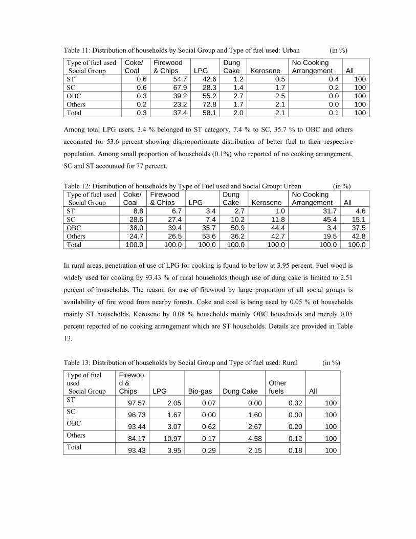
Table 11: Distribution of households by Social Group and Type of fuel used: Urban (in %)

Type of fuel used Social Group

Coke/Coal

Firewood & Chips LPG

Dung Cake Kerosene

No Cooking Arrangement All

ST 0.6 54.7 42.6 1.2 0.5 0.4 100SC 0.6 67.9 28.3 1.4 1.7 0.2 100OBC 0.3 39.2 55.2 2.7 2.5 0.0 100Others 0.2 23.2 72.8 1.7 2.1 0.0 100Total 0.3 37.4 58.1 2.0 2.1 0.1 100

Among total LPG users, 3.4 % belonged to ST category, 7.4 % to SC, 35.7 % to OBC and others

accounted for 53.6 percent showing disproportionate distribution of better fuel to their respective

population. Among small proportion of households (0.1%) who reported of no cooking arrangement,

SC and ST accounted for 77 percent.

Table 12: Distribution of households by Type of Fuel used and Social Group: Urban (in %) Type of fuel used Social Group

Coke/ Coal

Firewood & Chips LPG

Dung Cake Kerosene

No Cooking Arrangement All

ST 8.8 6.7 3.4 2.7 1.0 31.7 4.6SC 28.6 27.4 7.4 10.2 11.8 45.4 15.1OBC 38.0 39.4 35.7 50.9 44.4 3.4 37.5Others 24.7 26.5 53.6 36.2 42.7 19.5 42.8Total 100.0 100.0 100.0 100.0 100.0 100.0 100.0

In rural areas, penetration of use of LPG for cooking is found to be low at 3.95 percent. Fuel wood is

widely used for cooking by 93.43 % of rural households though use of dung cake is limited to 2.51

percent of households. The reason for use of firewood by large proportion of all social groups is

availability of fire wood from nearby forests. Coke and coal is being used by 0.05 % of households

mainly ST households, Kerosene by 0.08 % households mainly OBC households and merely 0.05

percent reported of no cooking arrangement which are ST households. Details are provided in Table

13.

Table 13: Distribution of households by Social Group and Type of fuel used: Rural (in %)

Type of fuel used Social Group

Firewood & Chips LPG Bio-gas Dung Cake

Other fuels All

ST 97.57 2.05 0.07 0.00 0.32 100SC 96.73 1.67 0.00 1.60 0.00 100OBC 93.44 3.07 0.62 2.67 0.20 100Others 84.17 10.97 0.17 4.58 0.12 100Total 93.43 3.95 0.29 2.15 0.18 100

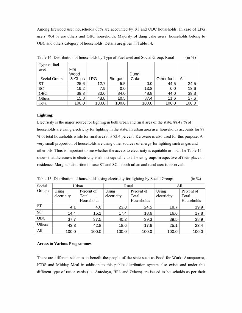
Among firewood user households 65% are accounted by ST and OBC households. In case of LPG

users 79.4 % are others and OBC households. Majority of dung cake users’ households belong to

OBC and others category of households. Details are given in Table 14.

Table 14: Distribution of households by Type of Fuel used and Social Group: Rural (in %)

Type of fuel used Social Group

Fire Wood & Chips LPG Bio-gas

Dung Cake Other fuel All

ST 25.6 12.7 5.5 0.0 44.5 24.5SC 19.2 7.9 0.0 13.8 0.0 18.6OBC 39.3 30.6 84.0 48.8 44.0 39.3Others 15.8 48.8 10.5 37.4 11.6 17.6Total 100.0 100.0 100.0 100.0 100.0 100.0

Lighting:

Electricity is the major source for lighting in both urban and rural area of the state. 88.48 % of

households are using electricity for lighting in the state. In urban area user households accounts for 97

% of total households while for rural area it is 83.4 percent. Kerosene is also used for this purpose. A

very small proportion of households are using other sources of energy for lighting such as gas and

other oils. Thus is important to see whether the access to electricity is equitable or not. The Table 15

shows that the access to electricity is almost equitable to all socio groups irrespective of their place of

residence. Marginal distortion in case ST and SC in both urban and rural area is observed.

Table 15: Distribution of households using electricity for lighting by Social Group: (in %)

Urban Rural All Social Groups Using

electricity Percent of Total Households

Using electricity

Percent of Total Households

Using electricity

Percent of Total Households

ST 4.1 4.6 23.8 24.5 18.7 19.9SC 14.4 15.1 17.4 18.6 16.6 17.8OBC 37.7 37.5 40.2 39.3 39.5 38.9Others 43.8 42.8 18.6 17.6 25.1 23.4All 100.0 100.0 100.0 100.0 100.0 100.0

Access to Various Programmes

There are different schemes to benefit the people of the state such as Food for Work, Annapoorna,

ICDS and Midday Meal in addition to this public distribution system also exists and under this

different type of ration cards (i.e. Antodaya, BPL and Others) are issued to households as per their

entitlement. An attempt is made to study the extent the reach of these programmes to the households

in the state.

State sample of 61st Round of NSSO reveals that Food for Work programme could reach to1.0 % of

households, Annapoorna 0.5 % households, ICDS 5.7 % and Midday Meal could reach 30.37 percent

of households in the state. Midday Meal could reach 35 percent of households in rural area while in

urban it was able to reach 13.5 % of households. It is also observed that programme could reach ST,

SC and OBC relatively more than state average reach. It is evident from Table 16 that programme

have targeted poor section of the society though with thin coverage. The percentage of beneficiary

households for each social group for urban and rural area is also presented below in Table 16.

Table 16: Reach of various programme by Social Groups (in %)

All (Urban+Rural) Social Groups Food for work Annapoorna ICDS Midday Meal

ST 2.0 0.4 6.0 38.96SC 1.3 1.5 6.2 34.91OBC 0.9 0.3 6.3 30.65Others 0.1 0.1 4.2 19.11All 1.0 0.5 5.7 30.37Table 16 continued

Urban Rural Social Groups Food

for work

Annapoorna ICDS Midday Meal

Food for work

Annapoorna ICDS Midday Meal

ST 1.19 0.00 1.07 7.60 2.0 0.4 6.3 40.7SC 0.42 1.42 1.11 27.96 1.5 1.5 7.4 36.6OBC 0.30 0.08 2.06 17.16 1.0 0.3 7.5 34.5Others 0.09 0.01 0.15 5.82 0.2 0.2 7.1 28.7All 0.27 0.25 1.05 13.50 1.2 0.5 7.1 35.4

Under Food for Work programme, it is observed that among total beneficiaries 96.9 % households

were from ST, SC and OBC category. Under Annpoorna Yojana, of the total benefited households

56.4 % were SC, followed by 22.9 % OBC and 15.6 % ST. Of the total who have availed the

services of ICDS, 42.8 % were OBC, followed by 21.0 % ST and 19.2 % SC. Midday Meal

programme, which has higher reach among the programmes under consideration, have 39.3 % of its

beneficiaries from OBC, 25.6 % from ST and 20.4 % from SC categories. The benefits are distributed

more in favour of poor section of the society. It is more or less true for urban and rural areas by

programme. The details are given in Table 17.

Table 17: Distribution of Beneficiaries by various programme and Social Groups (in %)

All (Urban+Rural) Social Groups Food for work Annapoorna ICDS Midday Meal

ST 39.6 15.6 21.0 25.6SC 22.6 56.4 19.2 20.4OBC 34.6 22.9 42.8 39.3Others 3.1 5.1 17.1 14.7All 100.0 100.0 100.0 100.0Table 17 continued

Urban Rural Social Groups Food for

work Annapoorna ICDS Midday

Meal Food for work

Annapoorna ICDS Midday Meal

ST 20.13 0.00 4.68 3.2 2.59 17.8 21.7 28.2SC 23.21 86.54 15.93 28.9 31.26 52.3 19.3 19.2OBC 42.22 12.03 73.37 50.3 47.70 24.4 41.4 38.3Others 14.44 1.42 6.03 17.6 18.45 5.6 17.5 14.3All 100.0 100.0 100.0 100.0 100.0 100.0 100.0 100.0

Ration Card Holding:

To provide subsidized food grain to the subjects belonging to poor section of the society, Food and

Civil Supply Department had issued different type of ration cards namely, Antodaya card, BPL card

and other cards. In some states, there are white, yellow and blue cards. In present context, Antodaya

card, BPL card and other card are being considered.

Survey results revealed that in state around 73 % of urban households, 83 % of rural households and

overall 80% of the households own ration card. Among social groups, highest proportion of SC

households (85.4 %) was holding ration cards in the state. It is true for both urban and rural areas. In

urban areas, it is followed by Others (73.5 %), OBC (71 %) and lowest proportion of household

owning ration card was ST with 68.3 %. In case of rural, after SC households second highest

proportion is observed for OBC household (83.7 %) followed by ST with 81.2 % and 79.9 % of other

households owned ration card. Proportion of Households holding Ration Card by social groups is

presented below in Table 18.

Table 18: Proportion of Households holding Ration Card (in %)

Social Group Urban Rural All ST 69.3 81.2 80.6 SC 76.6 87.5 85.4 OBC 71.2 83.7 81.0 Others 73.5 79.9 77.2 All 72.9 83.1 80.8

An attempt is made to study the pattern of holding of different type of ratio cards among ration card

holders. The over all distribution of ration cards among different social groups is almost evenly

distributed according to their population. The proportion of different type of ration cards among card

holders revealed that Antodaya card meant for the poorest among poor, accounts for merely 1.3

percent of the ration card holders and BPL card holders accounted for 25.2 percent while remaining

households owned other cards in the state. Percentage Distribution of cards by type for urban and

rural areas is also shown in Table 19. The holding of different type of ration cards is not evenly

distributed among groups because of the entitlements depends upon economic criterion. Among BPL

cards holder in urban areas, more than 65 % of BPL cards holder belongs to OBC and SC. In rural

areas, 90 % of BPL cards are held by other than Other households. In case of Antodaya Card, 99.4 %

of total cards are held by SC, ST and OBC in descending order while in urban areas 87 % of total

cards are owned by others, SC and ST. A detail distribution of different type of ration cards by social

classes is exhibited in Table 19. The pattern is found to be in line with the belief that SC, ST and

OBC’s constitute major chunk of poor population. The distribution of all type of cards among social

classes is evenly distributed to large extent irrespective of area of residence.

Table 19: Distribution of Different type of Ration Cards by Social Group (in %)

Social Group Antodaya BPL other All Type of cards

Urban ST 23.7 6.4 3.9 4.4SC 27.1 33.3 12.5 15.9OBC 19.9 32.0 37.6 36.6Others 29.4 28.3 46.0 43.1All 100.0 100.0 100.0 100.0Percentage Distribution of cards 0.5 15.7 83.8 100.0

Rural ST 32.5 33.7 20.0 24.0SC 45.8 28.8 15.4 19.5OBC 21.0 29.4 44.0 39.6Others 0.6 8.1 20.7 16.9All 100.0 100.0 100.0 100.0Percentage Distribution of cards 1.5 27.6 70.9 100.0

Total ST 31.8 30.2 16.2 19.9SC 44.4 29.4 14.7 18.8OBC 20.9 29.7 42.5 39.0Others 2.9 10.7 26.6 22.3All 100.0 100.0 100.0 100.0Percentage Distribution of cards 1.3 25.2 73.5 100.0

Expenditure Pattern and Inequality

Monthly Per Capita Expenditure:

The purpose of present analysis is not to estimate the extent of poverty prevailing in the state as per

61st Round of NSSO based on state sample. An attempt is made to study the relative position of

various social groups assuming different level of MPCE. Instead of 12 MPCE classes adopted by

NSSO, for the present study four MPCE classes have been formed by clubbing, in urban areas

monthly per capita expenditure classes adopted are less than Rs. 485, Rs. 485-930 and more than Rs.

930 which work out to less than Rs.16.16, 24.33 and more than Rs.31 per capita par day. For rural

area these classes are less than Rs. 455, Rs. 455-890 and more than Rs. 890 which work out to less

than Rs.15.16, 22.43 and more than Rs.30 per capita par day.

Results based on this analysis reveals that in urban areas there were 24.5 percent of total households

with MPCE less than Rs. 485. 28.1 % of households having MPCE more than Rs. 930 while

remaining 47.4 % of households having MPCE in range of Rs. 485 to Rs. 930. It is observed that

among SC households, the proportion of households with MPCE more than Rs.930 is lowest at 12.1

% followed by ST with 13.8 % and OBC with 21.1 %. It shows that majority of SC households (87.9

%) are incurring consumer expenditure less than Rs. 24 per capita per day on an average basis. The

proportion of similar households in ST and OBC categories are 86.2 % and 78.9 % respectively.

Among other households such households constitute for 58.5 % of total households. Details are

presented in Table 20.

Distribution of Households by Social Classes and MPCE class: Urban

41.145.1

13.8

44.4 43.5

12.1

29.9

49

21.1

10.9

47.6

41.5

24.5

47.4

28.1

0

10

20

30

40

50

60

< Rs. 485 Rs. 485 - 930 > Rs. 930

Perc

ent

ST SC OBC Others All

Table 20: Distribution of Households by Social Classes and MPCE class: Urban

MPCE Class Social Class

< Rs. 485 Rs. 485 - 930 > Rs. 930 All

ST 41.1 45.1 13.8 100.0 SC 44.4 43.5 12.1 100.0 OBC 29.9 49.0 21.1 100.0 Others 10.9 47.6 41.5 100.0 All 24.5 47.4 28.1 100.0

It is equally important to know that in each MPCE class who the major constituents are. Table 21

gives the distribution of households within each MPCE class. It reveals that around three fourth of

total households with MPCE less than Rs. 485 belong to OBC and ST categories. The distribution of

households in MPCE class of Rs. 485 to Rs. 930 shows that to large extent is same as their proportion

in total population. Highest category of MPCE (i.e. more than Rs. 930) is dominated by “Other

Households”. It shows that significantly good proportion of SC, OBC and ST are relatively not better

off than other households.

Table 21: Distribution of Households by Social Classes and MPCE class: Urban

MPCE Class Social Class

< Rs. 485 Rs. 485 - 930 > Rs. 930 All

ST 7.7 4.4 2.3 4.6SC 27.4 13.8 6.5 15.1OBC 45.8 38.8 28.2 37.5Others 19.1 43.0 63.1 42.8All 100.0 100.0 100.0 100.0

The other parameter to be studied is the average per capita consumer expenditure per day so that

intake differential if any can be highlighted. Table 22 reveals, that ST households belonging to MPCE

category of Rs. 485-930 are spending more than (on an average basis) households of other socio

groups and all households. OBC households are spending more as compare to (on an average basis)

other socio groups in lower and higher MPCE classes. This table also reveals that in urban areas SC

households are consuming less than their counterparts in each category of MPCE class except the

lower MPCE class where their average consumption is higher than that of ST households. Households

of Lower MPCE class of less than Rs. 485 are spending less than one fourth of their respective

counter parts in higher MPCE class except in case of SC households who are spending 29 percent and

ST households who are spending 21 percent of their counterparts in higher MPCE class. ST

households of lower MPCE class are spending less than half than their counter parts in next higher

MPCE class of Rs. 485 to Rs. 930 while for other socio groups it varies between 56 to 59 percent. It is

observed that average spending per day per person is higher in case of other households with Rs.

30.84 followed by OBC households (Rs. 24.15 ), ST households (Rs. 20.77) and least is for SC

households with Rs. 18.75 per capita per day. Households of MPCE class of less than Rs. 485 are

spending little more than half of average spending of all the households of same socio group except

Other households who are spending slightly less than half of the average spending of all other

households.

Table 22: Average Per Capita Per Day Expenditure by Social Classes and MPCE class: Urban

(in Rs. 0.00)

MPCE Class Social Class

< Rs. 485 Rs. 485 - 930 > Rs. 930 All

ST 11.17 23.90 52.06 20.77SC 12.20 20.63 41.43 18.75OBC 13.00 22.05 50.05 24.15Others 12.72 22.66 50.28 30.84All 12.59 22.21 49.69 26.10

Results based on this analysis reveals that in rural areas there were 44.5 percent of total households

with MPCE less than Rs. 455. Merely 7.9 % of households having MPCE more than Rs. 890 while

remaining 47.6 % of households having MPCE in range of Rs. 455 to Rs. 890. It is observed that

among other households, the proportion of households with MPCE more than Rs.890 is highest at

17.1 % followed by OBC with 9.3 % and ST with 3.2 %. It also reveals that majority of SC

households (97.8 %) are incurring consumer expenditure less than Rs. 22.43 per capita per day on an

average basis. The proportion of similar households in ST and OBC categories are 96.8 % and 90.7 %

respectively. Among other households such households constitute for 83.9 % of total households.

Thus large proportion of rural households are living in much worse conditions as compare to urban

households. Details are presented in Table 23.

Table 23: Distribution of Households by Social Classes and MPCE class: Rural (in %)

MPCE Class Social Class

< Rs. 455 Rs. 455 - 890 > Rs. 890 All

ST 59.8 37.0 3.2 100 SC 62.7 35.1 2.2 100 OBC 36.8 53.9 9.3 100 Others 21.3 61.6 17.1 100 All 44.5 47.6 7.9 100 Table 24 gives the distribution of households within each MPCE class. It reveals that around two third

of total households with MPCE less than Rs. 455 belong to OBC and ST categories. The distribution

of households by MPCE classes shows that households are not equitably distributed according to their

proportion in total population thus showing the disparity.

Table 24: Distribution of Households by Social Classes and MPCE class: Rural (in %)

MPCE Class Social Class

< Rs. 455 Rs. 455 - 890 > Rs. 890 All

ST 32.9 19.1 9.9 24.5SC 26.2 13.7 5.1 18.6OBC 32.5 44.5 46.6 39.3Others 8.4 22.7 38.4 17.6All 100.0 100.0 100.0 100.0 The other parameter to be studied is the average per capita consumer expenditure per day so that

intake differential if any can be highlighted. Table 25 reveals that ST and SC households are spending

less than average spending of all households irrespective of MPCE class. OBC and Other households

are spending more as compare to all households put together. Households of Lower MPCE class of

less than Rs. 455 are spending around one third of their counter parts in higher MPCE class and 60 %

of those in middle MPCE class of Rs. 455 to Rs. 890 irrespective of social class. This table also

reveals that in rural areas among SC and ST households intake is below the state average.

Table 25: Average Per Capita Per Day Expenditure by Social Classes and MPCE class: Rural

(in Rs. 0.00)

MPCE Class Social Class

< Rs. 455 Rs. 455 - 890 > Rs. 890 All

ST 11.52 18.60 35.01 14.25 SC 11.75 19.76 33.63 14.71 OBC 12.19 20.32 37.71 18.47 Others 12.58 21.12 38.56 21.66 All 11.89 20.15 37.71 17.37

Now question arises whether among different social groups, the proportion of households for different

consumption levels have similar pattern or not. To analyse this aspect, in urban area the consumption

level assumed are below Rs300, Rs. 350, Rs. 400, Rs450, Rs. 500, Rs. 550 and Rs. 600 while in rural

areas first four level have been considered. This analysis will reveal that an increment in consumption

level by Rs.50 what proportion of total households get included. In other word, these households can

be treated as target group which can be moved from one category of consumption class to another by

some interventions comparatively of smaller magnitude than moving all the households belonging to

lower MPCE class for which interventions of larger magnitudes are required.

Table 26 reveals that 19.28 % of ST population in the urban areas has MPCE less than Rs. 300 while

10.690% of SC population has same level of MPCE. In case of OBC and Others merely 1.62 % of

their population has MPCE less than Rs. 300. In case one considers MPCE classes less than Rs. 450

and more than Rs. 450, then different scenario emerge, which shows that the higher proportion of ST

population as compare to other socio groups is living with less than Rs. 450 monthly per capita

expenditure. While among those who are living with more than Rs. 450 monthly per capita

expenditure, higher percentage of SC population as compare to other socio groups is covered under

such category. In Figure 1 an attempt is made to reveal that with increment of Rs. 50 in MPCE class

the proportion of household get added through relative height of bar for different classes and socio

groups. This chart reveals that with each additional increase of Rs. 50 in MPCE relatively higher

proportion of population is affected. In case of ST population considerably high proportion of

population moved from MPCE level of Rs.400 to Rs. 450. While in case of OBC population such

movement of population is observed at slower pace in number of MPCE classes.

Table 26: Proportion of Population/Households below MPCE: Urban MPCE classes

MPCE less than

Social Group 300 350 400 450 500 550 600 ST Population (%) 19.28 29.72 33.06 43.17 46.88 50.54 51.39Households (%) 14.69 23.58 27.10 38.20 41.10 44.71 45.45SC Population (%) 10.69 18.21 28.75 40.04 51.54 59.12 68.02Households (%) 10.00 16.66 26.91 38.48 48.09 54.25 63.65OBC Population (%) 1.62 7.17 17.43 26.68 34.46 44.16 52.66Households (%) 1.60 6.67 15.30 24.80 31.86 40.18 47.89Others Population (%) 2.23 3.46 7.02 10.56 15.13 23.20 27.96Households (%) 2.07 3.14 6.23 9.34 12.42 18.09 21.72All Population (%) 4.10 8.21 15.29 22.40 29.19 37.59 44.20Households (%) 3.73 7.45 13.71 20.86 26.42 33.06 38.96

Figure 1

Proportion of Population below Different Level of Comnsumption (Rs. MPCE): Urban

19.3

10.7

1.6 2.24.1

29.7

18.2

7.23.5

8.2

33.1

28.7

17.4

7.0

15.3

43.240.0

26.7

10.6

22.4

46.9

51.5

34.5

15.1

29.2

50.5

59.1

44.2

23.2

37.6

51.4

68.0

52.7

28.0

44.2

0.0

10.0

20.0

30.0

40.0

50.0

60.0

70.0

80.0

ST SC OBC Others TotalSocial Group

Prop

ortio

n of

Pop

ulat

ion

300350400450500550600

Table 27 reveals that 16.40 % of ST population in the rural areas has MPCE less than Rs. 300 while

13.51% of SC population has same level of MPCE. In case of OBC and Others only 6.60 % and 2.61

% of their population has MPCE less than Rs. 300. The higher proportion of SC and SC population is

found for all MPCE classes under consideration as compare to OBC and Others. In Figure 2 reveals

that with each additional increase of Rs. 50 in MPCE relatively higher proportion of population is

affected. In case of ST and SC population considerably high proportion of population moved from

first MPCE level to the level of Rs.350 to Rs. 450. While in case of OBC population such movement

of population is observed is smaller in number of MPCE classes. This exercise can be used to target

specifically identified group of population through various programmes meant for eradication of

poverty. Even this analysis may help the planner to set the targets at various level to achieve pre set

overall goals.

Table 27: Proportion of Population/Households below MPCE: Rural MPCE classes

MPCE less than

Social Group 300 350 400 450 ST Population (%) 16.40 31.53 48.40 63.59 Households (%) 14.24 27.18 43.89 58.05 SC Population (%) 13.51 31.61 48.78 63.98 Households (%) 13.22 30.46 47.14 61.42 OBC Population (%) 6.60 14.53 26.64 38.24 Households (%) 5.81 13.50 25.00 35.71 Other Population (%) 2.61 6.63 13.18 21.75 Households (%) 2.00 4.81 11.60 19.64 All Population (%) 9.47 20.24 33.38 45.93 Households (%) 8.58 18.47 31.39 43.13

Figure 2:

Proportion of Population below Different Level of Consumption (Rs. MPCE): Rural

16.4013.51

6.602.61

9.47

31.53 31.61

14.53

6.63

20.24

48.40 48.78

26.64

13.18

33.38

63.59 63.98

38.24

21.75

45.93

0.00

10.00

20.00

30.00

40.00

50.00

60.00

70.00

ST SC OBC Others Total

Social Group

Prop

ortio

n of

Pop

ulat

ion

300350400450

Now targeting a particular category with given parameter keeping oneself within the limit of available

resources can be done easily provided one know how much amount is required to uplift the population

from one category to another. For this purpose average poverty gap has been calculated for each

MPCE class for Urban and Rural population by social groups and is presented in Tables 28 and Table

29. The relative expenditure to bring all the households with MPCE less than Rs. 450 to next MPCE

class will be more in rural areas than urban areas. Relative expenditure will be more for ST, SC and

others households of urban areas.

Table 28: Average Poverty Gap: Urban

(Amount required in bringing above present MPCE Class to Next Higher MPCE Class)

Amount required to bring above present MPCE Class to Next Higher MPCE Class

(Rs. Per month) Social Groups 300 350 400 450 500 550 600ST Per person 6.03 10.31 17.39 21.51 28.90 35.82 44.55Per household 37.29 61.18 99.92 114.52 155.25 190.73 237.26SC Per person 6.53 10.93 14.02 18.31 22.18 27.87 32.41Per household 35.97 61.62 77.29 98.27 122.60 156.66 178.64OBC Per person 9.39 7.35 9.20 13.69 18.88 22.95 27.67Per household 47.27 39.34 52.21 73.41 101.79 125.68 151.57Other Per person 4.64 10.14 11.15 14.65 16.87 17.70 21.37Per household 25.82 57.83 64.93 85.69 106.39 117.49 142.33All Per person 6.29 9.54 11.73 15.80 20.01 23.46 27.88Per household 35.07 30.28 66.44 86.14 112.25 135.48 160.63

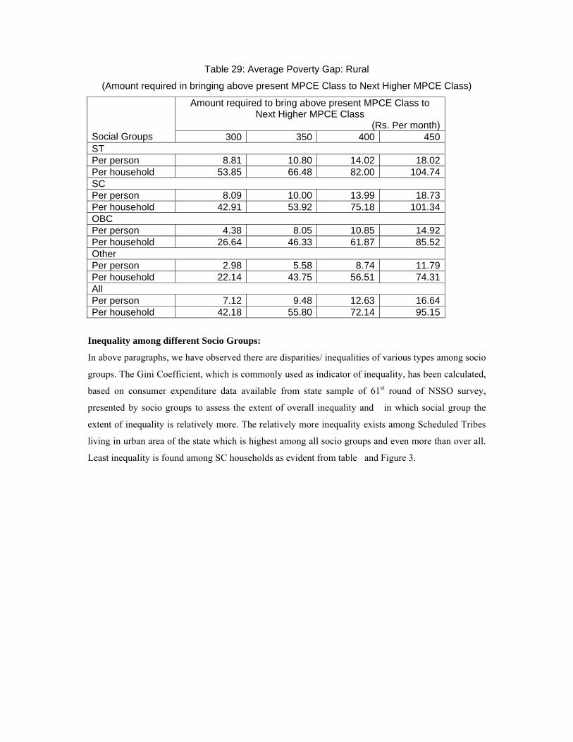
Table 29: Average Poverty Gap: Rural

(Amount required in bringing above present MPCE Class to Next Higher MPCE Class)

Amount required to bring above present MPCE Class to Next Higher MPCE Class

(Rs. Per month) Social Groups 300 350 400 450 ST Per person 8.81 10.80 14.02 18.02 Per household 53.85 66.48 82.00 104.74 SC Per person 8.09 10.00 13.99 18.73 Per household 42.91 53.92 75.18 101.34 OBC Per person 4.38 8.05 10.85 14.92 Per household 26.64 46.33 61.87 85.52 Other Per person 2.98 5.58 8.74 11.79 Per household 22.14 43.75 56.51 74.31 All Per person 7.12 9.48 12.63 16.64 Per household 42.18 55.80 72.14 95.15

Inequality among different Socio Groups:

In above paragraphs, we have observed there are disparities/ inequalities of various types among socio

groups. The Gini Coefficient, which is commonly used as indicator of inequality, has been calculated,

based on consumer expenditure data available from state sample of 61st round of NSSO survey,

presented by socio groups to assess the extent of overall inequality and in which social group the

extent of inequality is relatively more. The relatively more inequality exists among Scheduled Tribes

living in urban area of the state which is highest among all socio groups and even more than over all.

Least inequality is found among SC households as evident from table and Figure 3.

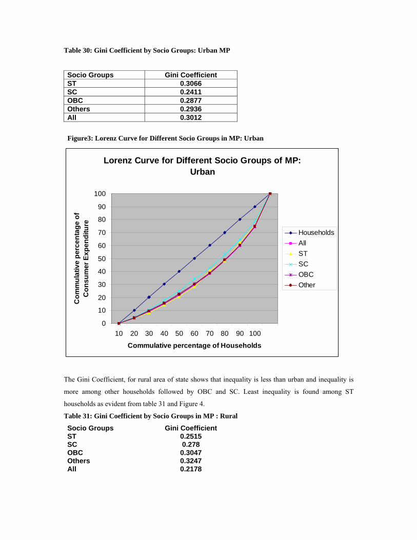
Table 30: Gini Coefficient by Socio Groups: Urban MP

Socio Groups Gini Coefficient ST 0.3066 SC 0.2411 OBC 0.2877 Others 0.2936 All 0.3012

Figure3: Lorenz Curve for Different Socio Groups in MP: Urban

Lorenz Curve for Different Socio Groups of MP: Urban

0

10

20

30

40

50

60

70

80

90

100

10 20 30 40 50 60 70 80 90 100

Commulative percentage of Households

Com

mul

ativ

e pe

rcen

tage

of

Con

sum

er E

xpen

ditu

re

HouseholdsAllSTSCOBCOther

The Gini Coefficient, for rural area of state shows that inequality is less than urban and inequality is

more among other households followed by OBC and SC. Least inequality is found among ST

households as evident from table 31 and Figure 4.

Table 31: Gini Coefficient by Socio Groups in MP : Rural

Socio Groups Gini Coefficient ST 0.2515 SC 0.278 OBC 0.3047 Others 0.3247 All 0.2178

Figure 4: Lorenz Curve for Different Socio Groups in MP: Rural

Lorenz Curve for Different Socio Groups in MP: Rural

0

10

20

30

40

50

60

70

80

90

100

0 10 20 30 40 50 60 70 80 90 100

Commulative Percentage of Households

Com

mul

ativ

e Pe

rcen

tage

of C

onsu

mer

Expe

nditu

re

ALLSTSCOBCOtherHouseholds

Other indicators such as poverty gap index and squared poverty gap index for various MPCE Classes

are presented below separately for Urban and Rural area separately.

Table 32: Poverty Gap Index for different MPCE classes by Socio-Groups: Urban

Socio groups MPCE <=300

MPCE <=350

MPCE <=400

MPCE <=450

MPCE <=500

MPCE <=550

MPCE <=600

ST Population (%) 0.39 0.88 1.44 2.06 2.71 3.29 3.82 Households (%) 1.83 4.12 6.77 9.72 12.76 15.50 17.97 SC Population (%) 0.23 0.57 1.01 1.63 2.29 3.00 3.67 Households (%) 1.20 2.93 5.20 8.40 11.79 15.45 18.95 OBC Population (%) 0.05 0.15 0.40 0.81 1.30 1.84 2.43 Households (%) 0.25 0.75 2.00 4.04 6.49 9.18 12.10 Other Population (%) 0.03 0.10 0.20 0.34 0.51 0.75 1.00 Households (%) 0.18 0.52 1.01 1.78 2.64 3.86 5.15 All Population (%) 0.09 0.22 0.45 0.79 1.17 1.60 2.05 Households (%) 0.44 1.14 2.28 3.99 5.93 8.14 10.43

Table 33: Squared Poverty Gap Index for different MPCE classes by Socio-Groups: Urban

Socio groups MPCE <=300

MPCE <=350

MPCE <=400

MPCE <=450

MPCE <=500

MPCE <=550

MPCE <=600

ST Population 1.75 4.08 8.57 13.89 19.76 25.78 31.68 Households 5.67 19.21 40.36 65.40 93.09 121.40 149.22 SC Population 0.70 2.63 5.94 10.45 15.97 22.43 29.57 Households 3.63 13.58 30.62 53.87 82.38 115.69 152.52 OBC Population 0.15 0.43 1.21 2.97 6.06 10.28 15.54 Households 0.74 2.14 6.04 14.81 30.20 51.22 77.41 Other Population 0.10 0.66 1.57 2.84 4.39 6.32 8.76 Households 0.54 3.41 8.13 14.68 22.70 32.70 45.31 All Population 0.26 1.02 2.41 4.52 7.44 11.08 15.42 Households 1.32 5.20 12.22 22.97 37.76 56.25 78.31

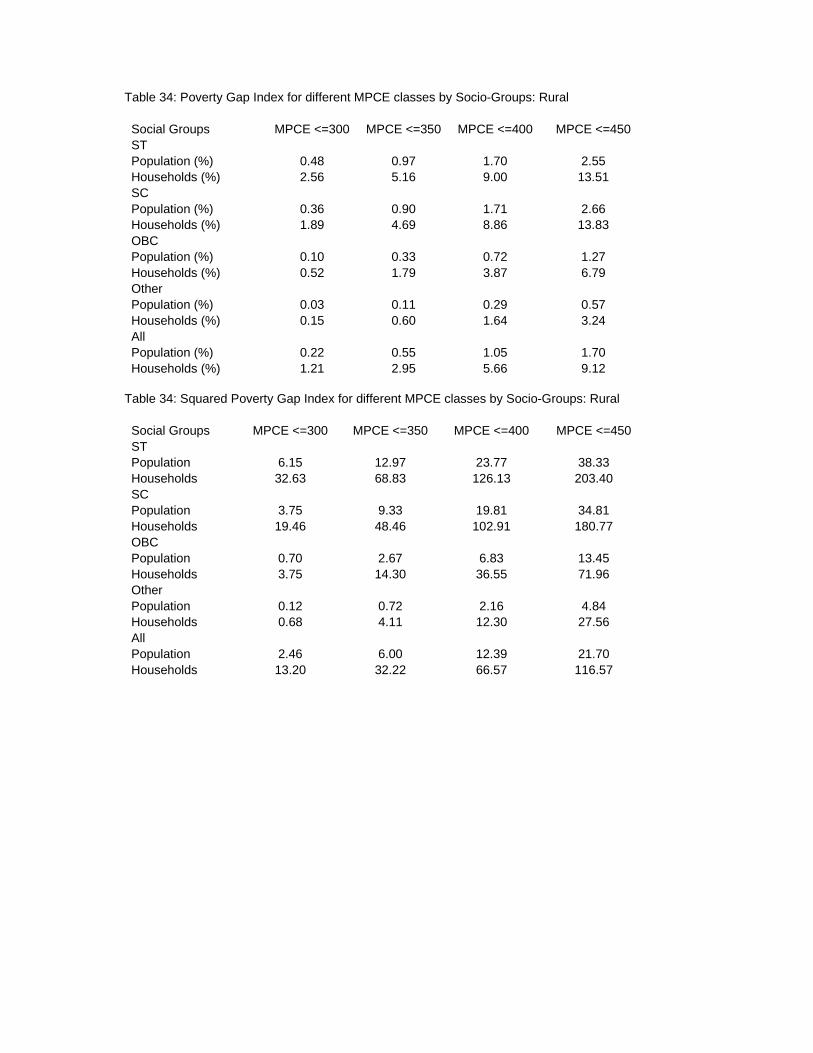
Table 34: Poverty Gap Index for different MPCE classes by Socio-Groups: Rural

Social Groups MPCE <=300 MPCE <=350 MPCE <=400 MPCE <=450 ST Population (%) 0.48 0.97 1.70 2.55 Households (%) 2.56 5.16 9.00 13.51 SC Population (%) 0.36 0.90 1.71 2.66 Households (%) 1.89 4.69 8.86 13.83 OBC Population (%) 0.10 0.33 0.72 1.27 Households (%) 0.52 1.79 3.87 6.79 Other Population (%) 0.03 0.11 0.29 0.57 Households (%) 0.15 0.60 1.64 3.24 All Population (%) 0.22 0.55 1.05 1.70 Households (%) 1.21 2.95 5.66 9.12

Table 34: Squared Poverty Gap Index for different MPCE classes by Socio-Groups: Rural

Social Groups MPCE <=300 MPCE <=350 MPCE <=400 MPCE <=450 ST Population 6.15 12.97 23.77 38.33 Households 32.63 68.83 126.13 203.40 SC Population 3.75 9.33 19.81 34.81 Households 19.46 48.46 102.91 180.77 OBC Population 0.70 2.67 6.83 13.45 Households 3.75 14.30 36.55 71.96 Other Population 0.12 0.72 2.16 4.84 Households 0.68 4.11 12.30 27.56 All Population 2.46 6.00 12.39 21.70 Households 13.20 32.22 66.57 116.57

Annexure Sample Design

Outline of sample design: A stratified multi-stage design has been adopted for the 61st round

survey. The first stage units (FSU) are the 2001 census villages in the rural sector and Urban

Frame Survey (UFS) blocks in the urban sector. The ultimate stage units (USU) are

households in both the sectors. In the case of large villages/blocks requiring hamlet-group

(hg)/sub-block (sb) formation, one intermediate stage is the selection of two hgs/sbs from

each FSU.

Sampling Frame for First Stage Units: For the rural sector, the list of 2001 census villages

(panchayat wards for Kerala) constitutes the sampling frame. For the urban sector, the list

of latest available Urban Frame Survey (UFS) blocks has been considered as the sampling

frame.

Stratification: Within each district of a State/UT, two basic strata have been formed: i) rural

stratum comprising of all rural areas of the district and (ii) urban stratum comprising of all the

urban areas of the district. However, if there are one or more towns with population 10 lakhs

or more as per population census 2001 in a district, each of them will also form a separate

basic stratum and the remaining urban areas of the district will be considered as another basic

stratum. There are 27 towns with population 10 lakhs or more at all-India level as per census

2001.

Sub-stratification:

Rural sector: If ‘r’ be the sample size allocated for a rural stratum, the number of sub-strata

formed is ‘r/2’. The villages within a district as per frame have been first arranged in

ascending order of population. Then sub-strata 1 to ‘r/2’ have been demarcated in such a way

that each sub-stratum comprises a group of villages of the arranged frame and has more or

less equal population.

Urban sector: If ‘u’ be the sample size for a urban stratum, ‘u/2’ number of sub-strata have

been formed. The towns within a district, except those with population 10 lakhs or more,

have been first arranged in ascending order of population. Next, UFS blocks of each town

have been arranged by IV unit no. × block no. in ascending order. From this arranged frame

of UFS blocks of all the towns, ‘u/2’ number of sub-strata has been formed in such a way that

each sub-stratum has more or less equal number of UFS blocks.

For towns with population 10 lakhs or more, the urban blocks have been first arranged

by IV unit no. × block no. in ascending order. Then ‘u/2’ number of sub-strata has been

formed in such a way that each sub-stratum has more or less equal number of blocks.

Total sample size (FSUs): 12784 FSUs have been allocated at all-India level on the basis of

investigator strength in different States/UTs for central sample and 14992 for state sample.

Allocation of total sample to States and UTs: The total number of sample FSUs is

allocated to the States and UTs in proportion to population as per census 2001 subject to the

availability of investigators ensuring more or less uniform work-load.

Allocation of State/UT level sample to rural and urban sectors: State/UT level sample

size is allocated between two sectors in proportion to population as per census 2001 with 1.5

weightage to urban sector subject to the restriction that urban sample size for bigger states

like Maharashtra, Tamil Nadu etc. should not exceed the rural sample size. A minimum of 8

FSUs has been allocated to each state/UT separately for rural and urban areas.

Allocation to strata: Within each sector of a State/UT, the respective sample size is

allocated to the different strata in proportion to the stratum population as per census 2001.

Allocations at stratum level have been adjusted to a multiple of 4 with a minimum sample

size of 4.

Selection of FSUs: Two FSUs have been selected from each sub-stratum of a district of rural

sector with Probability Proportional to Size With Replacement (PPSWR), size being the

population as per Population Census 2001. For urban sector, two FSUs have been selected

from each sub-stratum by using Simple Random Sampling Without Replacement

(SRSWOR). Within each sub-stratum, samples have been drawn in the form of two

independent sub-samples in both the rural and urban sectors.

Selection of hamlet-groups/sub-blocks/households - important steps

Criterion for hamlet-group/sub-block formation: Large villages/blocks having

approximate present population of 1200 or more will be divided into a suitable number (say,

D) of ‘hamlet-groups’ in the rural sector and ‘sub-blocks’ in the urban sector as stated below.

approximate present population

of the sample village/block

no. of hgs/sbs to

be formed (D)

less than 1200 (no hamlet-groups/sub-blocks) 1

1200 to 1799 3

1800 to 2399 4

2400 to 2999 5

3000 to 3599 6

…………..and so on

For rural areas of Himachal Pradesh, Sikkim and Poonch, Rajouri, Udhampur, Doda districts

of Jammu and Kashmir and Idukki district of Kerala, the number of hamlet-groups formed is

as follows.

approximate present population

of the sample village

no. of hgs to

be formed

less than 600 (no hamlet-groups) 1

600 to 899 3

900 to 1199 4

1200 to 1499 5

.………..and so on

Two hamlet-groups/sub-blocks are selected from a large village/UFS block wherever

hamlet-groups/sub-blocks have been formed, by SRSWOR. Listing and selection of the

households are done independently in the two selected hamlet-groups/sub-blocks. In case

hamlet-groups/sub-blocks are to be formed in the sample FSU, the same would be done by

more or less equalizing population.

Formation of Second Stage Strata and allocation of households

For both Schedule 1.0 and Schedule 10, households listed in the selected

village/block/ hamlet-groups/sub-blocks are stratified into three second stage strata (SSS) as

given below.

Rural: The three second-stage-strata (SSS) in the rural sector are formed in the following

order:

SSS 1: relatively affluent households

SSS 2: from the remaining households, households having principal

earning from non- agricultural activity

SSS 3: other households

Urban: In the urban sector, the three second-stage strata (SSS) are formed as under:

Two cut-off points, say ‘A’ and ‘B’, based on MPCE of NSS 55th round, have been

determined at NSS Region level in such a way that top 10% of households have MPCE more

than ‘A’ and bottom 30% have MPCE less than ‘B’. Then three second-stage-strata (SSS) are

formed in the urban sector in the following order:

SSS 1: households with MPCE more than A (i.e. MPCE > A)

SSS 2: households with MPCE equal to or less than A but equal to or

more than B ( i.e. B ≤ MPCE ≤ A)

SSS 3: households with MPCE less than B (i.e. MPCE < B)

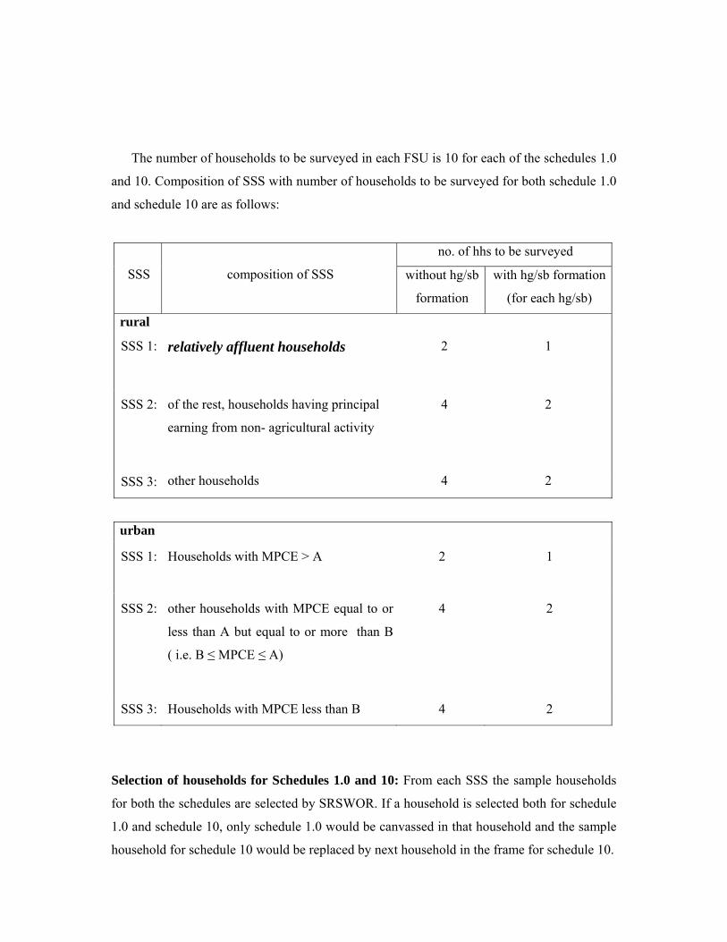
The number of households to be surveyed in each FSU is 10 for each of the schedules 1.0

and 10. Composition of SSS with number of households to be surveyed for both schedule 1.0

and schedule 10 are as follows:

no. of hhs to be surveyed

SSS composition of SSS without hg/sb

formation

with hg/sb formation

(for each hg/sb)

rural

SSS 1: relatively affluent households

2 1

SSS 2: of the rest, households having principal

earning from non- agricultural activity

4 2

SSS 3: other households 4 2

urban

SSS 1: Households with MPCE > A

2 1

SSS 2: other households with MPCE equal to or

less than A but equal to or more than B

( i.e. B ≤ MPCE ≤ A)

4 2

SSS 3: Households with MPCE less than B 4 2

Selection of households for Schedules 1.0 and 10: From each SSS the sample households

for both the schedules are selected by SRSWOR. If a household is selected both for schedule

1.0 and schedule 10, only schedule 1.0 would be canvassed in that household and the sample

household for schedule 10 would be replaced by next household in the frame for schedule 10.

Estimation Procedure

Notations:

s = subscript for s-th stratum

t = subscript for t-th sub-stratum

m = subscript for sub-sample (m =1, 2)

i = subscript for i-th FSU [village (panchayat ward) / block]

d = subscript for a hamlet-group/sub-block (d = 1, 2)

j = subscript for j-th second stage stratum in an FSU/ hg/sb ( j = 1, 2 or 3)

k = subscript for k-th sample household under a particular second stage stratum within an

FSU/ hg/sb

D = total number of hg’s/sb’s formed in the sample village (panchayat ward) / block

D* = 1 if D = 1

= D / 2 for FSUs with D > 1

N = total number of FSUs in any urban sub-stratum

Z = total size of a rural sub-stratum (= sum of sizes for all the FSUs of a rural sub-stratum )

z = size of sample village used for selection.

n = number of sample village / block surveyed including zero cases but excluding casualty

for a particular sub-sample and sub-stratum.

H = total number of households listed in a second-stage stratum of a village/block/hamlet-

group/sub-block of sample FSU

h = number of households surveyed in a second-stage stratum of a village/block/hamlet-

group/sub-block of sample FSU

x, y = observed value of characteristics x, y under estimation

X , Y = estimate of population total X, Y for the characteristics x, y

Under the above symbols,

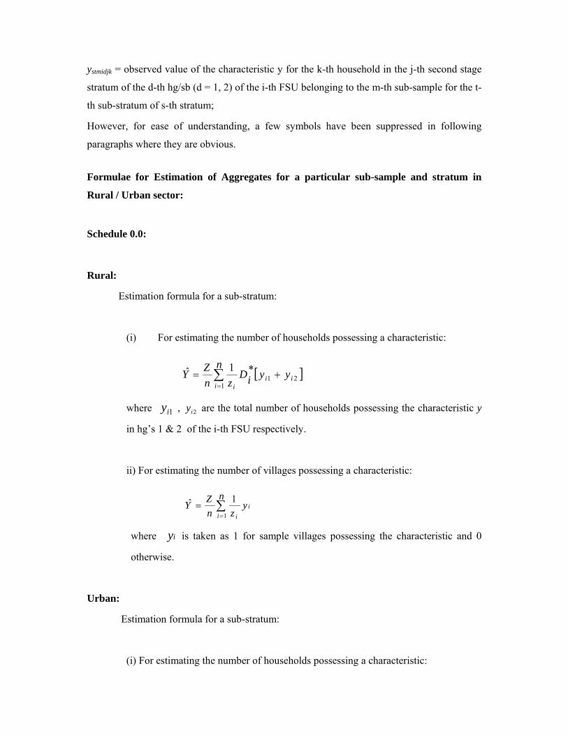
ystmidjk = observed value of the characteristic y for the k-th household in the j-th second stage

stratum of the d-th hg/sb (d = 1, 2) of the i-th FSU belonging to the m-th sub-sample for the t-

th sub-stratum of s-th stratum;

However, for ease of understanding, a few symbols have been suppressed in following

paragraphs where they are obvious.

Formulae for Estimation of Aggregates for a particular sub-sample and stratum in

Rural / Urban sector:

Schedule 0.0:

Rural:

Estimation formula for a sub-stratum:

(i) For estimating the number of households possessing a characteristic:

[ ]∑=

+=n

yyiDzn

ZYi

iii1

21*1ˆ

where 1iy , 2iy are the total number of households possessing the characteristic y

in hg’s 1 & 2 of the i-th FSU respectively.

ii) For estimating the number of villages possessing a characteristic:

∑=

=n

yzn

ZYi

ii1

1ˆ

where iy is taken as 1 for sample villages possessing the characteristic and 0

otherwise.

Urban:

Estimation formula for a sub-stratum:

(i) For estimating the number of households possessing a characteristic:

[ ]∑=

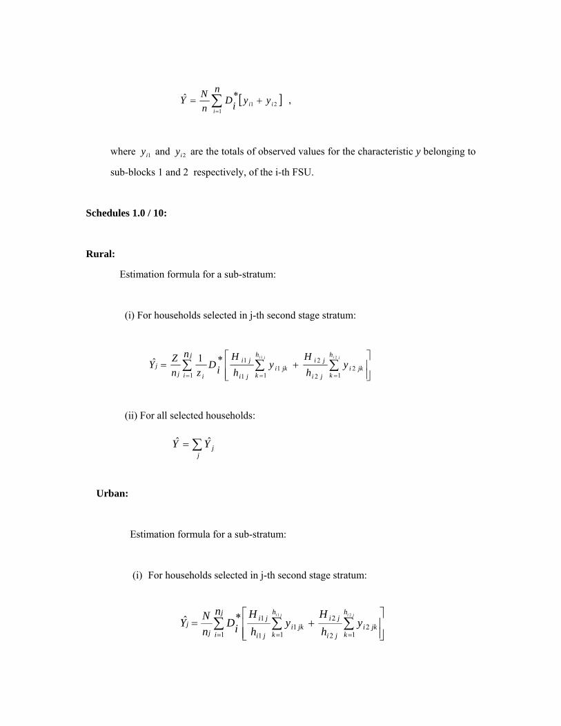
+=n

yyiDnNY

iii

121

*ˆ ,

where 1iy and 2iy are the totals of observed values for the characteristic y belonging to

sub-blocks 1 and 2 respectively, of the i-th FSU.

Schedules 1.0 / 10:

Rural:

Estimation formula for a sub-stratum:

(i) For households selected in j-th second stage stratum:

∑ ∑∑= == ⎥

⎥⎦

⎤

⎢⎢⎣

⎡+=

j

i

h

kjki

ji

jih

kjki

ji

ji

ijj

ny

hH

yhH

iDzn

ZYjiji

1 12

2

2

11

1

1 21*1ˆ

(ii) For all selected households:

∑=j

jYY ˆˆ

Urban:

Estimation formula for a sub-stratum:

(i) For households selected in j-th second stage stratum:

∑ ∑∑= == ⎥

⎥⎦

⎤

⎢⎢⎣

⎡+=

j

i

h

kjki

ji

jih

kjki

ji

ji

jj

ny

hH

yhH

iDnNY

jiji

1 12

2

2

11

1

1 21*ˆ

(ii) For all selected households:

∑=j

jYY ˆˆ

Estimate for a stratum:

∑=t

stYsY ˆˆ

Overall Estimate for Aggregates:

Overall estimate for aggregates for a stratum ( sY ) based on two sub-samples is obtained

as:

∑=

=2

1

ˆ21ˆ

msms YY

Overall Estimate of Aggregates at State/UT/all-India level:

The overall estimate Y at the State/ UT/ all-India level is obtained by summing the

stratum estimates sY over all strata belonging to the State/ UT/ all-India.

Estimates of Ratios:

Let Y and X be the overall estimate of the aggregates Y and X for two

characteristics y and x respectively at the State/ UT/ all-India level.

Then the combined ratio estimate )ˆ(R of the ratio )(XYR = will be obtained as

X

YR ˆ

ˆˆ = .

Estimates of Error: The estimated variances of the above estimates will be as follows:

For aggregate Y :

∑=s

sYraVYraV )ˆ(ˆ)ˆ(ˆ

where )ˆ(ˆ sYraV are as given below.

For strata with PPSWR selection at first stage:

⎥⎦

⎤⎢⎣

⎡−

−= ∑ ∑

=t

st

ist

sti

stist

ststsppswr

nY

zYZ

nnYraV

1

2)ˆˆ(

)1(1)ˆ(ˆ ,

where ∑=j

stijsti YY ,

⎥⎥⎦

⎤

⎢⎢⎣

⎡+= ∑∑

==

jiji h

kjki

ji

jih

kjki

ji

jististij y

hH

yhH

DY21

12

2

2

11

1

1*ˆ

For strata with SRSWOR selection at first stage:

( ) ( )∑ −=t

ststssrswor YYYrVa2

21ˆˆ

41ˆˆ ,

where 1stY and 2stY are the estimates for sub-sample 1 and sub-sample 2 respectively

for stratum ‘s’ and sub-stratum ‘t’.

For ratio R :

⎥⎦⎤

⎢⎣⎡ += ∑∑

′′

ss

ss RESMRESM

XRESM )ˆ(ˆ)ˆ(ˆ

)ˆ(1)ˆ(ˆ

2

where s, s' indicate respectively the strata with PPSWR and SRSWOR selection at first

stage.

For strata with PPSWR selection at first stage:

∑ ∑=

⎥⎦⎤

⎢⎣⎡ −−−

−=

t

st

istststisti

sti

st

ststs

nXRYXRY

zZ

nnRESM

2

1)ˆˆˆ()ˆˆˆ(

)1(1)ˆ(ˆ

where

∑=j

stijsti YY ˆˆ , ∑=j

stijsti XX ˆˆ ,

⎥⎥⎦

⎤

⎢⎢⎣

⎡+= ∑∑

==

jsijsi h

kjki

ji

jih

kjki

ji

jististij y

hH

yhH

DY21

12

2

2

11

1

1*ˆ ,

⎥⎥⎦

⎤

⎢⎢⎣

⎡+= ∑∑

==

jsijsi h

kjki

ji

jih

kjki

ji

jististij x

hH

xhH

DX21

12

2

2

11

1

1*ˆ

For strata with SRSWOR selection at first stage:

( ) ( ) ( )( )∑ ⎥⎦⎤

⎢⎣⎡ −−−−+−= ′′′′′′′′′

ttstststststststss XXYYRXXRYYRESM 2121

2

2122

21ˆˆˆˆˆ2ˆˆˆˆˆ

41)ˆ(ˆ

where 1ˆ

tsY ′ and 2ˆ

tsY ′ are the estimates for sub-sample 1 and sub-sample 2 respectively

for stratum ‘s'’ and sub-stratum ‘t’.

Estimates of RSE:

( ) ( )100ˆ

ˆˆˆˆ ×=Y

YraVYESR

( ) ( )100ˆ

ˆˆˆˆ ×=

R

RESMRESR

Multipliers:

The formulae for multipliers for a sub-sample and schedule type are given below:

formula for multipliers sch

type sub-stratum

hg / sb 1 hg / sb 2

0.0 Rural *1

stmistmistm

st Dzn

Z×× *1

stmistmistm

st Dzn

Z××

formula for multipliers sch

type sub-stratum

hg / sb 1 hg / sb 2

Urban *stmistm

st DnN *

stmistm

st DnN

rural

jstmi

jstmistmi

stmistmj

st

hH

Dzn

Z

1

1*1×××

j = 1, 2, 3

jstmi

jstmistmi

stmistmj

st

hH

Dzn

Z

2

2*1×××

j = 1, 2, 3 1.0 /

10

Urban jstmi

jstmistmi

stmj

st

hH

DnN

1

1* ×× ,

j = 1, 2, 3

jstmi

jstmistmi

stmj

st

hH

DnN

2

2* ×× ,

j = 1, 2, 3

Note: (i) For estimating any characteristic for any domain not specifically considered in

sample design, indicator variable may be used.

(ii) Multipliers have to be computed on the basis of information available in the

listing schedule irrespective of any misclassification observed between the listing

schedule and detailed enquiry schedule.

(iii) For estimating number of villages possessing a characteristics, *stmiD = 1 in the

relevant multipliers and there will be only one multiplier for the village.

Treatment for zero cases, casualty cases etc.:

While counting the number of FSUs surveyed (nstm ) in a sub-stratum, all the FSUs with

survey codes 1 to 6 in schedule 0.0 will be considered. In addition, if no SSU is available in

the frame for a particular schedule then also that FSU will be treated as surveyed in respect of

that schedule. However, if the SSUs of a particular schedule type are available in the frame

of the FSU but none of these could be surveyed then that FSU has to be treated as casualty

and it will not be treated as surveyed in respect of that schedule.

Casualty cases: FSUs with survey code 7 as per schedule 0.0 are treated as casualties. In

addition to this, an FSU, although surveyed, may have to be treated as casualty for a

particular schedule type and a particular second stage stratum as given in the following para:

FSUs with survey codes 1 and 4 as per schedule 0.0 having number of households in the

frame of j-th second stage stratum greater than 0 but number of households surveyed

according to data file, considering both hg/sb together, as nil (i.e. Hi1j + Hi2j >0 but hi1j + hi2j

=0) will be taken as casualties for j-th second stage stratum.

All the FSUs with survey codes 1 to 6 as per schedule 0.0 minus the number of

casualties as identified above will be taken as the number of surveyed FSUs (nstmj ) for that

sub-stratum × second stage stratum.

When casualty for j-th second stage stratum occurs for a particular hg/sb but not for the

other hg/sb, the FSU will not be treated as casualty but some adjustments in the value of H

for the other hg/sb will be done as follows:

(i) Suppose for hg/sb 1, Hi1j > 0 but hi1j = 0 while for hg/sb 2, Hi2j > 0 and hi2j > 0. In

that case jii HD 2* × will be replaced by )( 21

*jijii HHD +× in the formula for

multiplier of hg/sb 2.

(ii) Suppose for hg/sb 1, Hi1j>0 and hi1j > 0 while for hg/sb 2, Hi2j>0 but hi2j=0. In that

case jii HD 1* × will be replaced by )( 21

*jijii HHD +× in the formula for multiplier of

hg/sb 1.

It may be noted that nstmj would be same for hg/sb 1 & 2 of an FSU.

Treatment in cases of void second-stage strata/sub-strata /strata/NSS region at FSU or

household level

A sub-stratum may be void because of the casualty of all the FSUs belonging to the sub-

stratum. This may occur in one sub-sample or in both the sub-samples. If it relates to only

one sub-sample, then estimate for the void sub-stratum may be replaced with the estimate as

obtained from the other sub-sample for the same sub-stratum.

When a sub-stratum is void in both the sub-samples, the following procedure is

recommended:

Case(I): Sub-stratum void cases at FSU levels (i.e. all FSUs having survey code 7):

i) If a rural sub-stratum is void then it may be merged with a sub-stratum having the

next higher population size class of villages within the same district. Sub-stratum 1

may be merged with sub-stratum 2, sub-stratum 2 with sub-stratum 3 and so on. If

last sub-stratum is void, it will be merged with the previous sub-stratum.

(ii) If an urban sub-stratum is void then it may be merged with the sub-stratum with

next higher number within the same district/stratum i.e. Sub-stratum 1 may be

merged with sub-stratum 2, sub-stratum 2 with sub-stratum 3 and so on. If last

sub-stratum is void, it will be merged with the previous sub-stratum.

iii) If all the sub-strata in a district are void, it may be excluded from the coverage of

the survey. The state level estimates will be based on the estimates of districts for

which estimates are available and remarks to that effect may be added in appropriate

places.

Case (II): Stratum void case at second stage stratum level (i.e. all the FSUs are

casualties for a particular second stage stratum):

An FSU may be a casualty for a particular second stage stratum although survey

code is not 7. If all the FSUs of a sub-stratum become casualties in this manner for a

particular second stage stratum, the sub-stratum will become void. In such cases, sub-

strata will be merged with other sub-strata for all the second stage strata as in Case (I)

above.

However, if whole district/stratum becomes void in this manner for a particular

second stage stratum, adjustment for this type of stratum void case may be done

according to the following guidelines.

The adjustment will be made involving other strata (within NSS region) of the

State/U.T. Suppose A, B, C and D are the four strata in the State/UT/Region and

stratum C is void for j-th second stage stratum. If ajY , bjY and djY are the aggregate

estimates for the strata A, B and D respectively, then the estimate cjY for stratum C

may be obtained as ⎟⎟⎠

⎞⎜⎜⎝

⎛×

++

++c

dba

djbjaj ZZZZYYY ˆˆˆ

where Za, Zb, Zc and Zd are the sizes of strata

A, B, C and D respectively.

Reference to the values of Zst, Nst, nst, zsti, Dsti, D*sti, Hsti1j, hsti1j, Hsti2j, hsti2j:

(a) Values of Zst, Nst and allotted nst for the whole round are provided for rural sector

and urban sectors.

(b) nst should not be taken from the tables. The values of nstm for each sub-sample are

to be obtained following the guidelines given in para 7 above. It includes uninhibited

and zero cases but excludes casualty cases.

(c) The value of zsti is to be taken from the column of sample list under the heading

“frame population”. Value of Dsti are to be taken from item 16 of block 1, sch 0.0.

Dsti* is to be calculated from the value of Dsi.

(d) Values of Hsti1j, Hsti2j are to be taken from col.(5), block 6 of sch 0.0 for respective

hg/sb.

(e) The value of hsti1j and hsti2j should not be taken from col (9), block 6 of sch.0.0. The

figures should be obtained by counting the number of households in the data file

excluding the casualty households.