REPORT OF THE 2016 SAILFISH STOCK ASSESSMENT (Miami, …

SAILFISH STOCK ASSESSMENT MEETING – MIAMI 2016

REPORT OF THE 2016 SAILFISH STOCK ASSESSMENT (Miami, USA – 30 May to 3 June 2016)

1. Opening, adoption of Agenda and meeting arrangements

The Meeting was held at the Rosenstiel School of Marine and Atmospheric Science, University of Miami, Miami,

USA from 30 May - 3 June 2016. Local arrangements were made by Dr. David Die with financial support of

NOAA through the Cooperative Institute of Marine and Atmospheric Studies (CIMAS). Dr. Paul de Bruyn, on

behalf of the ICCAT Executive Secretary, thanked the University of Miami for hosting the meeting and providing

all logistical arrangements.

Dr. Freddy Arocha, the Billfish Species Group Rapporteur, chaired the meeting. Dr. Arocha welcomed the meeting

participants (hereinafter “the Group”) and proceeded to review the Agenda which was adopted with minor changes

(Appendix 1).

The List of Participants is included as Appendix 2. The List of documents presented at the meeting is attached

as Appendix 3.

The following participants served as Rapporteurs for various sections of the report:

Section Rapporteurs

1 P. de Bruyn

2 J. Hoolihan, P. de Bruyn, G. Diaz, H. Perryman

3 M. Schirripa, R. Sharma, M. Lauretta, M. Fitchett, E. Babcock, B. Mourato

4 R. Sharma, C. Brown

5 F. Forrestal, J. Costa, F. Arocha

6 M. Perez Moreno, F. Arocha

7 P. de Bruyn

2. Summary of available data for assessment

2.1 Biology

2.1.1 Genetics

SCRS/2016/P/025 described preliminary results of a study investigating genetic differentiation among groups of

Atlantic sailfish. Mitochondrial DNA was compared using a 645 base pair sequence from the control region. So

far, analyses have been undertaken on samples from the western North Atlantic (Florida), Senegal, and Brazil

(Figure 1). An AMOVA comparison indicated a moderate to strong (Φst = 0.1020, p = 0.011) differentiation

between northern and southern hemispheres, and moderate differentiation (Φst = 0.0783, P = 0.010) between

eastern and western Atlantic samples. In pairwise comparisons, the largest population differentiation was observed

between the western North Atlantic (Florida) and African (Senegal) groups, and the smallest differentiation

between the Brazil and African (Senegal) groups (Table 1). Preliminary results suggest genetic stock structure

between both the eastern and western Atlantic, and northern and southern hemispheres. Further work is needed to

elucidate and confirm the presence of stock structure. Additional collection and analyses of samples from Côte

d’Ivoire, EU-Portugal, E-U-Spain, d Uruguay and Venezuela, are anticipated.

2.1.2 Distribution

SCRS/2016/099 used general additive models (GAMs) to predict the spatial distribution of sailfish across the Gulf

of Mexico (GOM) using data from the U.S. PLL Observer Program (2005-2010).

A delta approach fitting a Bernoulli GAM with binomial data, and a Gamma GAM with zero-truncated catch rate data (fish/100 hooks) was used. Model factors included year, season, day/night, sea bottom depth, altimetry, sea surface temperature, and minimum distance from a front. Results indicated that both the probability of catching a sailfish and the CPUE are most influenced by sea bottom depth and sea surface temperature. Seasonal distribution profiles were developed across the GOM by predicting across grids of NCEI and AVISO environmental data (Figure 2). Profiles indicated a seasonal flux, with increased sailfish CPUE between April and September, and higher catch rates associated to fronts.

1


2.1.3 Age, Growth, Natural Mortality and Maturity at size

The Group reviewed and compared growth parameters based on relevant information compiled from sailfish age

and growth studies conducted in the Atlantic and Pacific Oceans. Discussion and comparison of growth curve

estimates (Table 2, Figure 3) resulted in the Group’s conclusion that the growth trajectory estimated by

Cerdenares-Ladrón et al. (2011) was the most plausible, and agreement to use the following growth parameters in

the exploratory assessment model runs: Linf = 206.83; K = 0.36; T0 = -0.24.;

The Group discussed the estimate of M. It was noted that appropriate methods to estimate M based on tag-recapture

and maximum age were those described in Hoenig (1983) and in Then et al. (2015). Considering that the estimates

of M were high, the Group considered applying the estimate of M obtained using the method by Hoenig (1983)

and to be consistent with prior billfish stock assessments (BUM). Therefore, an estimate of M = 0.35 (based on

Hoenig equation from 1983) and a mean maximum age of 12 years was selected based on information available

from age and growth, and tagging information reviewed during the meeting.

It was noted to the Group that a new estimate of maturity at size was presented and discussed in the 2014

Intersessional meeting of the 2014 Billfish Species Group held in Mexico (Anon. 2015), and during the 2015 SCRS

Species Groups meeting (Anon. 2016), which resulted in an new L50 estimate of 142.12 cm LJFL (@ 3 years) by

the combination of Brazilian and Venezuelan reproductive samples to produce the new L50 estimate for west

sailfish.

2.2 Catch, effort, and size

The Task I nominal catch (T1NC) statistics of sailfish by stock, flag and gear, are presented in Table 3 and by

stock in Figure 4. The Secretariat informed the Group that updates were made to the historical catch series for

Venezuela (Longline artisanal).

The Group noted that for two key fisheries, data was either absent (Grenada) or the reported catches were extremely

low (Mixed flags (FR+ES)) in recent years. In the case of Grenada, the Group decided that for the assessment, an

average of the catch reported between 2007 and 2009 (the final three years of reported data from that CPC) would

be carried over for the years 2010 to 2014 (191t per year). For the Mixed flags fleet, estimates of the eastern stock

of sailfish caught as by-catch in the EU tropical tuna purse seine fleet were made by the Group using the stratified

ratio estimator method and the EU Purse Seine observer database. The observed sailfish by-catch were linearly

related to the observed tuna catch in both FAD and free sets. Observed sets and the tropical tuna catch from the

Task II database were stratified by year and fishing mode. By-catch ratio estimators for sailfish were calculated

using the mean observed sailfish by-catch in each stratum divided by the mean observed tuna catch for each

stratum. This ratio estimator was then applied to the total reported tuna catch for each stratum, yielding total

estimates of sailfish by-catch. The results from this analysis are presented in Tables 4a and b for FAD and free

school catches, respectively. The Group noted that this analysis indicates that the catches reported in the Task I

data are almost certainly lower than the true catches. As such, the Group decided for assessment purposes to use

the average of the catches reported between 2008 and 2010 as a carry over for the years 2011 to 2014 (275 t per

year).

The Group noted the strong decline in total reported sailfish catches since 2010. Although it was not clear how

accurate total captures were prior to this period, several potential factors may have resulted in decreased reporting

in recent years. For example, these reduced captures could potentially be a product of management actions or

changes in fishing operations (such as switches in targeting for many commercial longline vessels). With regards

to management, there may have been some reduction in sailfish captures due to the Billfish rebuilding plan which

was enacted in 2005. It was noted that this plan was only focused on marlin species but there was speculation that

this may have had an effect on sailfish catches as well. Related to this management action, the Group noted that

live release information is not provided and, thus, if management has discouraged retaining any billfish catches,

these potential releases have not been recorded. Very few fleets report any dead discard information for sailfish

and this makes the quantification of these potential captures impossible. The Group considered the possibility that

the recent decline of catches could be a result of increased, but unrecorded live releases and dead discards. Overall,

the Group expressed its concern that high uncertainty still remains with respect to total removals.

2


During the 2009 Sailfish Stock Assessment Session (Anon. 2010), it was reported that the catch and effort data

from Ghana used in the standardization of CPUE for the gillnet fishery had very different patterns in the

relationships between CPUE, trips and number of canoes when you compared data prior or after 1992. Such

differences led the Group in 2009 to exclude the Ghana CPUE data prior to 1992. Such pattern was also seen again

when the data were standardized in preparation for the current assessment (SCRS/P/2016/027). Furthermore, catch

levels prior and after 1990 are very different and prior to 1992 the species composition of billfish landings reported

by Ghana is very different to that prior to 1989. The Group concluded that catches of sailfish for Ghana between

1956 and 1989 may have been incorrectly estimated.

To test the sensitivity of assessment results to the estimates of sailfish catch from Ghana, an alternative catch series

of sailfish catches for Ghana for the period 1957-1989 was developed during the meeting (Appendix 4).

The data catalogues for sailfish regarding Task II catch and effort (T2CE) and Task II size information (T2SZ),

were presented to the Group for the Atlantic West and East stocks. This information is presented in Tables 5a and

5b respectively. The Group noted that many gaps exist in these datasets which limits the ability of the Group to

use integrated stock assessment models. The Group noted, however, that much data regarding size information

exists (especially for Venezuela) from the Enhanced Program for Billfish Research and the JDMIP (Arocha et al.

2016) and this data is being compiled for inclusion in the ICCAT database even though it is not official Task II

data submitted by the CPC. In addition, the Task II CE data is not often used in sailfish stock assessments as CPCs

usually provide standardised CPUE indices using more comprehensive data than is available in the Task II dataset.

The sailfish conventional tagging data available in the ICCAT database is presented in Table 6. There are a total

of 115,743 sailfish individuals released between 1950 and 2011. The total number of individuals recovered is

2,020, which represents on average a recovery ratio of about 1.7%. The apparent movement (straight displacements

between release and recovery positions) shown in Figure 5 (complemented by the release and recovery density

maps of Figure 6) indicates that the largest amount of the sailfish tagging took place in the western Atlantic. The

Group acknowledged the important work (national scientists and the Secretariat) behind the ICCAT tagging

database on sailfish and noted the large number of individuals that had been tagged. The Group recommended in

the future exploring methodologies to include this important information into the stock assessments framework.

2.3 Relative Indices of Abundance

The following documents with indices of abundance for the western stock were presented to the Group during

the meeting:

Document SCRS/2016/075 indicated that catches of sailfish (Istiophorus albicans), white marlin (Tetrapturus

albidus) and blue marlin (Makaira nigricans) and effort data were available from the recreational rod and reel

fishery based at the Playa Grande Yacht Club, Central Venezuela, from 1961 to 2001. Data were also available

from an artisanal drift-gillnet fishery in the same area from 1991 to 2014. Each dataset was standardized

independently using a generalized linear mixed model (GLMM). The two datasets were also combined in a GLMM

analysis that included the year, season, fishery and some two-way interactions as potential explanatory variables.

The combined analysis produced a CPUE index of abundance that runs from 1961 to 2014. The index shows a

decline followed by a period of stability for both sailfish and white marlin.

The Group inquired if trips with no catches were included in the analysis. It was indicated that the data for both

gears (recreational rod and reel and gillnet) corresponded to monthly summaries and that nearly all the monthly

summaries have positive catches. It was also discussed that since both fisheries are conducted in an area considered

to be a ‘hot spot’, the possibility of trip with no sailfish catch was extremely low. The Group noticed that some of

the model diagnostics showed some deviance from the assumptions. It was discussed that adding a constant value

to the model might have created the pattern seen in the residuals. Following the advice from the authors, the Group

agreed to use the individual indices instead of the combined index, as it was initially suggested in Babcock and

Arocha, 2015.

3


Document SCRS/2016/093 presented an index of abundance for sailfish from the United States recreational billfish

tournament fishery for the period 1972-2014 and for non-tournament recreational fisheries for the period 1981-

2014. Tournament catch-per-unit-effort (number of fish caught per 100 hours fishing) was estimated from catch

and effort data submitted by recreational tournament coordinators and U.S. National Marine Fisheries Service

observers under the Recreational Billfish Survey program. A selection process was applied to restrict the data to

tournaments that primarily target sailfish, using live bait only, along the Florida East coast. Non-tournament

recreational data was compiled from the Marine Recreational Fisheries Statistical Survey (MRFSS). The catch per

unit effort standardization procedure included the variables year, area, and season. Standardized indices were

estimated using Generalized Linear Mixed Models under a Delta lognormal model approach.

The authors explained that the data from MRFSS covered a larger area (the data included covered from the State

of North Carolina through Texas) than the tournament data, and therefore it was used to see if there was any

indication of the stock moving or expanding further north as it has been hypothesized for North Atlantic swordfish.

However, the authors indicated that there was no evidence of this being the case. The Group discussed the

difficulties in identifying the target species in the MRFSS data, which could affect the number of trips with zero

catches included in the analysis. It was also noted by the Group that the model diagnostics for the MRFSS index

showed strong evidence that the assumption of normality was violated. Therefore, the Group supported the

decision made in the 2009 Sailfish Stock Assessment Session (Anon. 2010) of not including the MRFSS index in

the 2016 Sailfish Stock Assessment and only including the tournament index.

Document SCRS/2016/092 catch and effort data from 73,810 sets done by the Brazilian tuna longline fleet,

including both national and chartered vessels, in the equatorial and southwestern Atlantic Ocean, from 1978 to

2012, were analyzed. The fished area was distributed along a wide area of the equatorial and South Atlantic Ocean,

ranging from 3º W to 52º W of longitude, and from 11º N to 40º S of latitude. The CPUE of the sailfish was

standardized by a Generalized Linear Mixed Model (GLMM) using a Delta Lognormal approach. The factors used

in the model were: year, fishing strategy, quarter, area, sea surface temperature, and the interactions year:strategy,

year:quarter and year:area. The standardized CPUE series of the sailfish showed a gradual decreasing trend,

particularly after the year 2000.

The Group asked the author how was the SST data used in the standardization obtained and it was indicated that

it was from satellite data. The Group also suggested that it is preferably to incorporate SST data into the models

as a categorical variable (bins) instead of as a continuous variable because many species have a range of preferred

temperatures and their response to temperature is not linear. As it was the cases with other species groups, the

Group held an extensive discussion with regard to the methodology used to define the three fishing strategies (FS).

The Group was concerned that the FS:Year interaction was significant which means that the catchability of those

3 FS changed with time. It was discussed that such effect might be masking true changes in stock abundance. As

a potential fix, the Group suggested to estimate individual CPUEs for each FS, or to do so only for the FS with the

highest mean CPUE. Alternatively, the Group also suggested to exclude the FS:Year interaction from the model.

If the nominal and the standardized CPUEs are similar then keeping the interaction in the model should not raise

much of a concern.

- The following documents with indices of abundance for the eastern stock were presented to the Group during the

meeting:

Presentation SCRS/P/2016/026 introduced a standardized index of abundance for the artisanal fishery in Senegal

for the period 1981-2015. The main gears in the fishery are troll, handline, and gillnet which incidentally catches

sailfish. The catch and effort data used corresponded to monthly summaries of catch and effort (n=1076). The

standardized index was estimated using a GLMM. The main factors tested in the model were year, area, month

and gear. Two models were considered, one with only the main factors and a second one with the main factors and

the interactions. Model selection was based on the AIC. The final model used to estimate the standardized index

included the factors year, area, gear, and month and the interactions year:area, year:gear, area:gear, and

gear:month. The estimated standardized index showed no discernible trend in the first 20 years of the time series

and a declining trend after year 2000.

The Group noted that monthly aggregated data was used in the analysis and the data used in the model

corresponded to the positive observations (N=1072 positive observations). The examination of the mean CPUE

by factor showed a consistency among the results and what is known about the fishery. More specifically, troll

gear has higher catches than seine gear (which targets sardines), and that highest catches occur during the

upwelling months. The significant Year:Month interaction supports the anecdotal observation that the length of

the period when sailfish are present in the area of the study has shortened. The Group noted that the estimated

4


CPUE for years 2013 and 2014 were significantly lower than the rest of the time series and the author indicated

that was the result of new management regulations. Therefore, the Group requested that the index be re-estimated

without including the last two years of data (2014-2015). A new estimated index without the last two years of data

was provided by the author during the meeting.

Presentation SCRS/P/2016/027 introduced a standardized index of abundance for the Ghanaian drift gillnet

artisanal fishery for the period 1974-2013. The data used corresponded to monthly summaries of catch and effort

data. No data for years 1983 and 2010 were included as part of the time series. The standardization procedure used

a GLM. The factors tested in the model were year, quarter, fishing season, number of canoes, and the interactions

Year:Quarter and Year:Fishing Season. The factors included in the final model were year, quarter, and the

interaction year:quarter. Although variable, highest CPUE values were observed in the late 80s and in the 90s. The

index values for the last three years of the time series (2011-2013) were the lowest since 1991. The Group requested

that a new split index for the periods 1974-1990 and 1991-2013 be estimated. Such indices were provided during

the meeting.

Document SCRS/2016/098 analyzed the catch, effort, and standardized CPUE trends for the eastern stock of

Atlantic sailfish (Istiophorus albicans) captured by the Portuguese pelagic longline fleet between 1999 and 2015.

Nominal annual CPUEs were calculated as kg/1000 hooks and were standardized with Generalized Linear Models

(GLM) with Tweedie distribution and using year, quarter, area, and targeting effects (ratios) as explanatory

variables. Model goodness-of-fit was determined with AIC and the pseudo coefficient of determination, and model

validation was analyzed with residual analysis. The final standardized CPUE series shows a general decrease in

the initial years, between 1999 and 2010, followed by a general increase in the more recent years, until 2015, with

some inter-annual oscillations. This paper presents the first index of abundance for Atlantic sailfish estimated from

captures from the Portuguese pelagic longline fleet in the east Atlantic and can be used for future stock assessments

of the species.

It was recommended by the Group that future versions of this index also include the estimated mean CPUE for

each factor in the model.

- The following documents with indices of abundance for both the eastern and western stocks were presented to

the Group during the meeting:

Document SCRS/2016/071 introduced standardized catch rates of the sailfish (Istiophorus albicans) obtained from

10,615 trip observations of EU-Spain surface longline fishing targeting swordfish during the period 2001-2014. In

roughly 28% of these trips at least one individual belonging to this species was found. Because of the low

prevalence of this species in this fishery, the standardized CPUE was developed using a Generalized Linear Mixed

Model assuming a delta-lognormal error distribution. The results obtained indicate that the overall trend of the

standardized CPUE was similar for the total Atlantic areas and for the East and West stocks. An overall increasing

trend was identified for the total Atlantic areas and for the East and West stock for the whole 2001-2014 period

with some fluctuations in the most recent years.

The Group inquired what was the rationale used to define the different areas used in the CPUEs standardization.

It was pointed out that the areas defined were similar to those used for the analysis of the same fleet for target and

other species, and they represent an approximation of the sea temperatures at 50 m depth. Other elements that were

also taken into consideration to define the spatial structure for the analysis included the current stock boundaries

assumed by ICCAT for this species, and environmental conditions in the surface layers between East and West

areas as well as North and South were also considered. Moreover, the distribution of the fleet in the respective

areas throughout the year and observations available also plays an important role in deciding the spatial-temporal

definitions for analysis. The Group agreed to use in the assessment the individual indices presented for each stock

(East and West) instead of the index also presented for the entire Atlantic.

Document SCRS/2016/094 presented estimated standardized CPUEs for sailfish caught by Japanese tuna longline

fishery in the western and eastern Atlantic Ocean using logbook data during 1994-2014. Delta lognormal model

was used to standardize the nominal CPUEs. Annual changes in the standardized CPUEs for the western Atlantic

stock showed a large fluctuation. The time series had a slight decreasing trend from 1994 to 2007 and after that

the time series had sharply increased and maintained at higher values. Annual changes in the standardized CPUEs

for the eastern Atlantic stock were considerably stable. The time series had a slight decreasing trend during 1994

and 2001, while the time series showed an increasing trend since then. The 95% confidence intervals were not

wide for the western and eastern Atlantic sailfish stocks. These results suggest that the current adult stock level of

sailfish in the western and eastern Atlantic increased in recent years compared with those in the 1990s and 2000s.

5


It was indicated by the authors that the use of the habitat model should be dismissed due to the lack of vertical

distribution information for sailfish. However, the Group noted that vertical distribution information has been

available since 2009 and recommended that this information be incorporated in the future. The Group noted that

the standardized index for the western stock was below the nominal index for the entire time series. It was discussed

that the indices start in 1994 because prior to that year the data did not separate catches of sailfish and spearfish.

In the 2009 Sailfish Stock Assessment Session (Anon. 2010), a JPN index that covered the period 1960-2007 was

included in the analysis. It was indicated to the Group that such index was developed during the assessment

meeting using CATDIS data and the estimated sailfish/spearfish ratios in the catch. The Group inquired if the

presence of spearfish in the estimated ratios was significant and it was informed that in some areas up to 30-40%

of the catches were spearfish. The Group noted that in eastern Atlantic, the Japanese longline fleet of yellowfin

catches in numbers were higher than bigeye catches when less than 15 hooks–between-float were used, while the

opposite was true when more than 15 hooks–between-float were used. However, the same trend was not evident

in the western Atlantic. The Group discussed the implication of these observations, but it was agreed that there

was not enough information available to interpret this particular results. The Group agreed to use in the assessment

the newly estimated index for each stock for the period 1994-2014 and use (as a separate index) the historical

CPUE estimated by the Group in the 2009 Sailfish Stock Assessment Session (Anon. 2010), only for the period

1960-1993. The Group noted that the strong year:area interaction and notably an apparent increase of catches in

the western Caribbean might require a finer spatial partitioning than the current coarse areas used in the model;

this could be the areas chosen by the adaptive partition method originally proposed in the document. To address

this concern, the index was split into two different periods in the stock synthesis model (see Section 3.2.3 for

details).

Document SCRS/2016/102 introduced catch and effort data of sailfish (Istiophorus platypterus) collected and

analyzed for the Chinese-Taipei distant-water longline fishery in the Atlantic Ocean for the period 2009-2015.

Catch in number observed in logbooks and that estimated using catch ratio of sailfish over the two species (sailfish

and spearfish Tetrapturus pfluegeri) were used to calculate nominal CPUE (catch per unit of effort), and then

CPUE was standardized using generalized linear models (GLMs). Two separate eastern and western stocks of

sailfish were considered in the standardization, with information on operation type (i.e., hooks per basket) included

as a potential effect in the models. All of the main effects were statistically significant in the GLM analyses, except

for month and longitude in the standardization of the western stock. However, relative abundance indices showed

similar and consistent trends for the two scenarios on catch data. The standardized CPUE of eastern Atlantic

sailfish increased from 2009 to a higher level but then dropped in recent two years (2014-2015), while for the

western stock the CPUE showed a decreasing trend during 2010 and 2014 with a slightly increase in 2015.

The Group noted that the data used did not include observations with zero catches. The author indicated that about

19% of the observations had sailfish positive catches and that the percentage was fairly constant. The Group

inquired how stable was the ratio sailfish-spearfish. It was indicated that the ratio was very variable since catches

for these species are a rare event. The author indicated that Logbook data was used to estimate the ratios by area

and it was assumed that the ratios remained constant with time. The Group indicated that the ratios might not have

been constant throughout the entire time series. However, with that assumption it should be possible to use the

ratios to estimate CPUE series prior to 2009.

The Group discussed the possibility of combining the data from the EU-Spain and EU-Portugal longline fisheries

to estimate a combined index for eastern sailfish, and potentially expand this approach to combine data from other

fleets. This approach of combining data from different fleets to estimate indexes of abundance is currently being

explored for other species like bluefin tuna. The Group acknowledged the importance of having standardized

indices from the artisanal fisheries of Senegal and Ghana, and those from EU-Spain and EU- Portugal longline

fisheries. The Group thanked the authors of these documents and their significant contribution to the assessment

process.

The Group also have available other indices of abundance that were presented at the 2014 Intersessional meeting

of the Billfish Group (Anon. 2015) and the 2015 SCRS Species Groups meeting (Madrid, 21-25 September 2015).

Tables 7 and 8 (and Figures 7 and 8) show the indices of abundance used for the western and eastern stocks,

respectively.

6


3. Stock Assessment

3.1 Eastern stock

3.1.1 Bayesian production models

Methods

For the eastern Atlantic population, Bayesian production models were run using both the BSP model that is

available from the ICCAT catalog of methods (BSP-VB, Babcock 2007, McAllister and Babcock 2003) and a

JAGS version of the same model based on Millar and Meyer (1999, BSP-JAGS). See Appendix 5 for details on

model specification, diagnostics and sensitivity analyses.

For all model runs, the prior for biomass in the first year relative to K (Bo/K) was lognormal with mean of 1 and

a CV of 0.2, except for a sensitivity that fixed Bo/K at 1. The prior for K was uniform on log(K) between log(10)

and log(1E6). The prior for r was calculated using the demographic method of Carruthers and McAllister (2011),

as shown in Appendix 6. Because the annual time step was used, the input parameters were a mean of 0.57, and

CV of 0.3. In a sensitivity analysis, the mean was set equal to 0.3 with a CV of 0.3. Uninformative priors were

used for the catchability coefficient for each CPUE index (q), using a uniform distribution in BSP-VP and an

inverse gamma distribution in BSP-JAGS. The same priors were used for the residual variance, in cases where

sigma was estimated.

None of the BSP-VB models included process error. For the BSP-JAGS models, process error was fixed at 0.05,

except in sensitivity runs in which sigma was set to either 0.00001 or 0 to evaluate the effect of removing process

error. The models varied in which indices were included, how the indices were weighted, and the priors for r and

Bo/K (Table 9). The indices included were either those that had an increasing trend (Chinese Taipei, EU- Japan-

early, Japan-late, Spain) or those that had decreasing trend (Côte d’Ivoire, EU-Portugal, Ghana, Japan-early,

Senegal). Indices were weighted equally with an estimated variance, or weighted by catch (input precision equal

to the fraction of the total catch associated with each index), or each index had its own estimated residual variance.

Results

The BSP-VB models without process error did not converge well, particularly for the case with an estimated

variance for each series. The Hessian estimate of variance for some parameters was near zero, although the

importance sampling estimated very wide distributions for the parameters indicating that the model may not have

accurately estimated the mode of the posterior distribution. The model posteriors were very similar to the priors

for both K and r, even though K had an uninformative prior. Thus, the mean values of K were orders of magnitude

higher than the values from other models applied to the same dataset. Because the model was unable to find any

information in the data, these model results are not credible. See Appendix 5 for details.

The BSP-JAGS models with process error provided better convergence diagnostics. The catch weighted models

gave posterior distributions for r that were quite similar to the priors (see Appendix 5), probably because the data

were given very low weights relative to the priors. Because of this, the results were highly uncertain, and the 95%

confidence intervals for B/BMSY included a range from near zero to more than 4 for some years (Table 10, Figure

9). The models that estimated residual variance provided more narrow credible intervals for B/BMSY and F/FMSY.

All the models other than the catch-weighted ones estimated a posterior mean of r that was higher than the prior;

these high r values may not be biologically realistic.

All of the models estimated a starting biomass that was below BMSY, probably because the models attempted to fit the large variability in the Japanese longline series in the 1960s combined with very low catches. All the runs were similar during the early part of the time series, but the runs with increasing versus decreasing indices diverged in recent years as the median biomass trajectory follows the indices. Estimates of MSY were between 5,000 t and 13,000 t, and the current stock status was below BMSY in all runs. That the population was depleted despite the fact that catches were never above MSY was surprising, but may be explained by the fact that the process error allowed the model to follow the decreasing trend in the indices despite the relatively low catches. Incorporating process error implies that biomass is allowed to vary randomly, without necessarily following the catch time series exactly. Thus, the population estimates could decline if the indices are declining, even if reported catches are low. Three possible scenarios that may explain this are: (1) that the reported catches are lower than real catches, (2) there is a decline in abundance not caused by catch, and/or (3) the actual MSY may be lower than the model estimate due to data uncertainty.

7


Current fishing mortality is below FMSY in some of the runs with increasing indices, and far above FMSY in the

models with decreasing indices. In general, the BSP-JAGS runs are consistent with a population that has declined,

and may or may not be rebuilding depending on which indices, if any, are tracking abundance. However, these

results are highly uncertain.

3.1.2 ASPIC

During the 2009 assessment ASPIC 5.0 was used for fitting production models for sailfish in the eastern Atlantic.

In this assessment, ASPIC 7.0 was used. Although ASPIC 7.0 allows for input of priors for initial parameters, this

option was not used in the present assessment for sailfish in the eastern Atlantic.

After examining the different indices available for the assessment of the eastern stock the Group agreed, similarly

to the approach used for the western stock, to group the indices into two different scenarios. One scenario contains

the indices that showed positive trends in the last years of the time series and the other scenario the indices that

showed negative trends. Additionally the Group agreed that the relative abundance index for Ghana should be split

into two series Ghana1 (1974-1987) and Ghana2 (1992-2014).

The following scenarios of CPUE indices were used in ASPIC runs:

E1) Recent trends in indices is negative: Japan1, Ghana1, Ghana2, Senegal, Côte d’Ivoire, EU-Portugal

(‘Neg’)

E2) Recent trends in indices is positive: Japan1, Japan2, Ghana1, EU-Spain, Chinese Taipei (‘Pos’)

E3) All indices: Chinese Taipei, Côte d’Ivoire, EU-Spain, Ghana1, Ghana2, Japan1, Japan2, Portugal,

Senegal

E4) Like E1 but with a recalculated catch for Ghana prior to 1990

E5) Like E3 but with a recalculated catch for Ghana prior to 1990

E6) Like E1 but with the Ghana CPUE as a single uninterrupted series

In all cases, CPUE indices were given equal weighting in the fit. As part of model diagnostics, retrospective

patterns were run by using data up to 2013, 2011, 2009 and 2007. Uncertainty was assessed by running 500

bootstraps in ASPIC.

Results

Estimates for FMSY, MSY, and K appear highly sensitive to the CPUE trends used, Therefore, results for different

scenarios were significantly different (e.g. E1 vs E2). ASPIC fits better the scenarios that omit data for the

period1988-1990 from the Ghana1 index and separate the Ghana series into two indices (E1-E5). ASPIC have

problem converging, or didn’t converge, for the scenarios with a single Ghana series (E6).

Runs that use CPUE with positive trends yielded different estimates of current biomass and exploitation than runs

that use CPUE with negative trends or all indices combined. However, fits and parameter estimates for FMSY, K,

and MSY with positive trajectories were highly sensitive to which catch series was used (Task 1 or alternative

Task I series) and fit observed indices quite poorly. Runs with alternative catch either did not converge or bounded

out at the upper limit of FMSY (1.5). Runs that use CPUE with negative trends and both Ghana series appeared the

least sensitive to the use of different catch series and exhibited the highest value of contrast in ASPIC. Furthermore,

historical trends of B/BMSY and F/FMSY for the period up to 2007 for scenarios are consistent with results from the

previous 2009 assessment.

Scenarios (E2 and E5) with recent positive trends did not fit the model and solutions kept hitting the upper

constraint of FMSY (1.5) (Table 11). It was considered that such high values are not biologically plausible and,

therefore, results for these scenarios were not considered any further.

The other two scenarios (E1 and E4) allowed the model to converge and both suggested that the stock is overfished

and is undergoing overfishing. Scenario E4 is more optimistic and suggested that in the last two years overfishing

is not occurring; while Scenario E1 indicated that overfishing continues.

For scenarios E2 and E5, deterministic results suggest the stock was previously overfished in prior decades and is

not presently undergoing overfishing, ASPIC Run E3 suggests that overfishing may have stopped over the last two

years and the stock is recovering.

8


Unfortunately, scenario E3 was not able to be bootstrapped so the only bootstrap results available are those for E1.

Retrospective analyses for E1 show what is expected from the addition of the recent CPUE data that show increases

in the index and catch data that show decreases (Figure 10). As data are added the Biomass estimates become

larger and the fishing mortality smaller. Boostraps for E1 converged for 100% of runs and yielded reasonable

intervals for parameters (Table 12).

E3 exhibits a retrospective pattern with great inconsistencies in the use of all indices for the recent 7 years. The

ASPIC run E3 produced results consistent to E1; however, using all indices create issues with consistency for

estimates of FMSY, B/BMSY, and F/FMSY (Figure 11).

3.2 Western stock

3.2.1 ASPIC

Production models were fitted for western sailfish using different combinations of the available indices of

abundance. The first model included all indices and was run with both ASPIC 5 and ASPIC 7 using the least

squares estimation method. Both software versions solved to the same solution; however, the estimates of FMSY

were not biologically plausible (FMSY>1.2). ASPIC 7 was used for all other model runs, using maximum likelihood

estimation or maximum a posterior with priors. Uniform priors were included for MSY and fleet catchabilities

across a range of logical values. A beta prior was included on FMSY (alpha=2, beta=8; Figure 12), based on the

prior developed for the Bayesian Surplus Production model for r. Multiple model runs were conducted using this

parameterization, which included multiple scenarios of selected indices: (1) all indices, (2) those which showed an

increasing trend in recent period, versus (3) those that showed a decreasing trend in the recent period, and (4) catch

weighting versus (5) equal indices weighting. A base model was selected by the Group which included all available

indices except the Brazilian rod and reel which was excluded due to concerns about extremely low samples sizes

in 2009. Multiple sensitivity runs were conducted on the base model, including an indices jackknife, model

bootstrap, and retrospective analysis. An additional run was made with the Japan longline index split at 2008 to

account for a change in spatial distribution (see section 2.3), consistent with the stock synthesis assessment model.

The base deterministic model runs showed poor model fit to the indices and a lack of convergence without prior

on FMSY, hitting the upper bounds on either FMSY or MSY. To better understand model convergence, the negative

log-likelihood objective function was profiled across the range of hypothesized MSY (200 to 4,000 t) and FMSY

(0.01 to 1.0) values. The profile surface indicated a flat contour at the upper ranges of MSY, and little gradient

across the range of FMSY (Figure 13). This profile across the range of logical parameter values demonstrated that

the ability to estimate FMSY was poor, and that values of MSY greater than 1,400 t are plausible. The scaled

likelihood surface (Figure 13) indicated the maximum likelihood at the upper bound of FMSY, which believed to

be biologically implausible.

Estimates of MSY and FMSY varied greatly between the different model runs, with little agreement between the

base model and alternative positive and negative indices models. Estimates of current stock status were also highly

variable with no agreement across models. Bootstrap estimates of parameter uncertainty were evaluated to

determine the quality of the fit of the base model. Many bootstrap runs bounded at the upper limit of MSY or FMSY;

however, these runs were overwritten with runs that solved within the bounds, until 500 valid bootstraps were

completed. Overall convergence was approximately 72% of trials. The resulting bootstrap estimate of FMSY and

MSY showed a wide distribution across the range of parameter bounds (Figure 14), indicating poor model

performance and lack of convergence to a stable solution. It was concluded that the ASPIC model for western

sailfish did not produce reliable estimates of FMSY or current stock status. The information in the data did indicate

that MSY is not likely to be less than 1,400 t; however, the determination of stock status was highly uncertain.

3.2.2 Bayesian state space surplus production model

SCRS/2016/103 presented initial results of the stock assessment of the western Atlantic sailfish. The assessment model was implemented in JAGS (Just Another Gibbs Sampler) and consisted of fitting a Bayesian state-space surplus production model to CPUE data for western Atlantic sailfish. The catch time series is derived from the Task I table in the 2015 SCRS Report (Anon. 2016) and relative abundance indices consisted of standardized catch-per-unit effort (CPUE) for Brazil, Chinese Taipei, EU-Spain, Japan, United States and Venezuela, including longline, recreational and gillnet fisheries. One run that included all input CPUE series (9 indices) and prior mean values was developed. The full specifications of the initial model presented are detailed in this SCRS document. Based on model outputs the western Atlantic sailfish population biomass has slightly declined over the available time series but it is above BMSY and has remained stable since middle 1980s. The estimated harvest rate in 2014 was 0.025, which is lower than the estimated HMSY of 0.065.

9


Several assumptions regarding data weighting, including equal weights, weights proportional to the catches and

weights developed by applying the Francis method (Francis, 2011) were considered. However, none of the models

could converge. A model with all indices together (except Brazilian recreational rod and reel fishery) was also

tested, but it did not converge either. This lack of convergence might be related to the presence of conflicting trends

in the CPUE. Thus, additional runs were performed to address the conflicting trends in the CPUEs in a similar way

as agreed for the Stock Synthesis model (see Section 3.2.3) which also resulted in a lack of convergence in all runs.

Also, the Group noted that the available data did not provide sufficient information for any of these models to

reliably estimate the model parameters.

3.2.3 Stock Synthesis (ASPM) 3 parameters, steepness, R0 and M

The initial model was presented (SCRS/2016/100) with the following details. Comparisons were made with the

old and new models on data used in the previous assessment and what was used in current years. In the 2009

assessment of the western stock, a composite index that was averaged across all series (weighted by-catch and

area) was used. In the current examination of the Age Structured Production Model (ASMP), 11 fleets were

modelled assuming full selectivity. It was noted that the CPUE series had conflicting trends, as five of the series

were increasing, and five were decreasing. This would cause conflicting results based on alternative trends. In the

model presented, no Brazilian Rod & Reel catches were available in recent years. A combined index was generated

based on catches and landings across fisheries (so larger fisheries got more weight). Four models/approaches were

examined, (1) unweighted CPUE with no recruitment deviates, (2) use all CPUEs with no recruitment deviates,

(3) add catch weighted with no recruitment deviates, and (4) add catch weighted CPUE and recruitment deviates.

It was noted that the results of model 1, 2 and 3 were not convincingly plausible, and model 4 results were more

consistent with the known history of the fishery. Likelihood profiling approaches were used, and the data were

found to be non-informative on natural mortality or steepness. It was noted that the Japanese and Spanish CPUE’s

were informative, though steepness very large or very low if it were fit to those series. Possible reasons for this are

that the CPUE data are not informative, and mostly a one way trip is evident. A new set of length/age structured

models were used, where the growth was modified as Priors, and size at age 1 was fixed at 100 cm LJFL. However,

trying to introduce more uncertainty with growth, provided an unrealistic answer.

Additional work was accomplished following that described in SCRS/2016/100. With the length composition data,

five models were examined that combined CPUE weighted by catch, 3 gears selectivity, gillnet, rod and reel and

longline, with bias correction to the stock-recruitment function used. The Dome shaped selectivity was used for

gillnet, the longline and rod and reel was fixed as a logistic. As per the 2009 assessment, one CPUE series was

generated where the combined CPUE was applied across all fisheries. The Length Composition data resulted in a

better fit to the gillnet fleet than longline fleet, due mostly to the larger sample size of the gillnet fishery which

resulted in that data series getting a higher weighting (based on the Francis weighting scheme; Francis, 2011).

Mean length fits to the gillnet gear and longline gear were acceptable, but not so much for the Rod & Reel fishery

(again because of the low sample size). Profiling on steepness indicated the overall data/model ‘preferred’ a very

high steepness and natural mortality values (M). In addition, the posteriors were similar to MLE’s analyzed.

The Group discussed the different inputs of the model and particularly whether the western sailfish catches were

recorded completely and/or accurately. In addition, it was noted that in previous sailfish meetings the Group have

not adopted growth and M estimates, and that additional time should be used by the Group to decide on an

appropriate estimate of M and a growth curve. It was also noted that fixing M and steepness (h) would have a

strong influence on the outcome of the estimates of stock productivity. As a result, the posteriors distributions of

the –MCMC may be misleading and should be viewed with appropriate skepticism. For example, the steepness

appeared to be estimated at the upper bound. In addition, all information on ASPM comes from the CPUE’s.

Given the conflicting CPUE time series and no means to objectively discern which of the trends were more accurate, it was suggested that two separate models for the two separate scenarios (alternative hypothesis) be constructed, one represented by only the CPUE’s with increasing trends (Model_1) and another by only the CPUE’s with decreasing trends (Model_2). While the size frequency data was seen as informative, improving the fit was not a worthwhile pursuit. The Group agreed that the use of a combined index (across all conflicting CPUE time series) would be hiding the uncertainty associated to the different CPUEs trends and that models should be constructed that use data across all CPUE series, rather than one series, and be transparent with the datasets being used.

10


A long discussion ensued and the Group agreed to group the CPUEs based on the prevailing trend in the time

series, which resulted in the following groupings (Figure 15):

1. Those with increasing trends:

a) Japan longline, 1994-2015

b) US rod and reel tournaments

c) Venezuela gillnet

d) Spanish longline

2. Those with decreasing trends:

a) Brazil rod and reel

b) Brazil longline

c) US longline (observer)

d) Venezuela longline

e) Chinese Taipei recent (2009-2014)

3. Those used in both data sets based on being the only long term time series:

a) Japan longline 1960-1993

b) Venezuela Rod and Reel

The input biological population parameters for the SS model are those discussed and agreed in Section 2.1 under

the item on Age, Growth, Natural Mortality and Maturity at Size.

Model_1.0 and Model_2.0

The Group examined two scenarios, one based on positive (Model_1.0) and another on negative (Model_2.0)

trending CPUEs. The standard deviation on the steepness prior was tightened from 20% to 10%. Both scenarios

were considered plausible with different datasets. It was noted that the fits to the survey index (CPUEs) were

comparable across the two different scenarios (Figure 15). Estimated and observed mean lengths from gillnet and

rod and reel fisheries were comparable, but were better for the longline fishery from Model_1 (Figure 16). It was

noted that the average size of fish in the gillnet fishery declined (Figure 17). A larger sample and less variable

sizes were observed and as such, created tighter fits of the selectivity to the length information. Longline fleets

changing selectivity over time are a possible reason why the model was not fitting the data very well.

It was noted that the two models agreed in the stock biomass trend fairly well up until the year 2005. This was

because the last few data points of the CPUE time series had a large influence on biomass trajectories. One model

(Model_1) suggests a high fishing mortality and lower biomass, and the other (Model_2) vice-versa (Figure 18).

As a mean to further differentiate between the two scenarios a retrospective analysis was suggested for each as a

diagnostic. An examination of the retrospective analysis showed no retrospective pattern or bias apparent for

Model_1. However, Model_2 showed a strong difference in biomass estimates when excluding data after 2010.

However, it was noted that recent upward trend in Model_1 was being driven by the Japanese (recent) CPUE as

well as the U.S. rod and reel index. The recent declining trend in Model_2 was being driven almost entirely by

the Brazilian rod and reel index (Figure 19).

Model_1.1 and Model_2.1

Given the strong influence on the current perception of stock status driven by the Japanese longline index

(Model_1.0) and the Brazilian rod and reel index (Model_2.0) the Group revisited the fundamentals of these two

CPUE time series.

Model_1.1. Two observations were made regarding the Japanese CPUE times series. The first observation was

that there was a marked increase in the index between 2007 and 2008. The second observation was that the CV’s

associated with the second stanza of this index (2008-2014) were much smaller than the first stanza (1994-2007).

These two aspects resulted in the assessment model making a large jump in the estimates of biomass between 2007

and 2008. The small CV’s for the second stanza accentuated the fit to this jump. The Group determined that it

would be appropriate to let catchability change between the two periods by using time blocks in CPUE series for

the Japanese series (in effect breaking it into two surveys). Effects of having a catchability change indicates that

the models performed better than the previous models, and recruitment deviates are not exceedingly large (Figure

20).

11


Model_2.1. The Group then discussed the sudden drop in biomass in recent years as estimated by the Brazilian rod

and reel index. Closer examination of this index revealed that the 2009 data point was being estimated from only

three sampling days. The Group concluded that this point was unlikely to be representative and also influenced the

standardization of the other annual estimates of relative biomass. In addition, the Group was unable to estimate an

alternative index excluding the 2009 data during this meeting and, therefore, decided to exclude the entire index

from further analysis. Once removed, no retrospective patterns or bias was evident (Figure 21). Furthermore, the

two scenarios were much more in agreement with each other, at least with regard to the current status of the stock

(Figure 20). The Group made a final examination of the four candidate models (Model_1, 2, 1.1, and 2.1), and

made the determination to adopt Model_1.1 and Model_2.1 as two plausible scenarios to represent the current

status of the stock.

In an effort to further refine the plausibility of the two candidate models chosen above, MCMC analysis was

conducted on each of the estimated parameters and the deterministic estimate of stock status (i.e. F/FMSY and

B/BMSY) compared to the distribution of stock status evaluations from the MCMC analysis. A total of 501,000

MCMC runs were made with the first 1,000 runs being discarded as a “burn in” period. The remaining runs were

thinned by 1,000 resulting in a total of 5000 runs for analysis. Examination of the MCMC distributions of

Model_1.1 showed that the median of the posterior values of the steepness parameter was being estimated

considerably higher (approximately 0.90) than the informative prior value used (0.70) (Figure 22). The distribution

of the posteriors was rather tight relative to the distribution of the prior, suggesting a strong signal in the data for

a higher steepness value. Three of the gillnet selectivity parameters were well estimated, as evidenced from the

“normal” shape of the posterior distributions, while two were not, either resulting in a uniform distribution

(parameter number 1) or one highly skewed to the left (parameter number 6). The resulting Kobe plot from

Model_1.1 showed that while the point estimates of stock status were in the green zone (neither overfished or

under going over fishing), the MCMC cluster of points were 87% in the red zone (both overfished and under going

over fishing) (Figure 23). This disparity in results makes any perception of stock status highly uncertain.

Examination of the MCMC distributions of Model_2.1 posteriors suggested that the median value of steepness

was closer (approximately 0.8) to that of the prior (0.7) and had a shape that would be expected from that parameter

(beta-like) (Figure 24). The estimates of the gillnet selectivity parameters were similar to those of Model_1.1. The

resulting Kobe status plot had more desirable diagnostics than Model_1.1 in that the point estimate of the 2014

status was within the 95% confidence intervals of the MCMC, however not within the 75% confidence intervals

(Figure 25). The point estimate of stock status from Model_2.1 suggested the stock is neither overfished or under

going over fishing; however, the centroid of the MCMC cluster suggests the stock is in the red zone (both

overfished and under going over fishing) (Figure 24). This disparity in results makes any perception of stock status

from Model_2.1 also uncertain.

3.3. SRA Section (Catch-MSY Methods)

In standard stock assessments conducted in the Atlantic, indices of abundance are essential elements to capture

trends in biomass over time. For Sailfish in the Atlantic, CPUE data showed conflicting trends in both the eastern

and the western stocks and, therefore, the Group attempted a catch only method. The primary method used is a

technique called Stock reduction Analysis (Zhou et al. 2012, Walters et al. 2006, Martell and Froese 2012, Kimura

and Tagart 1982) which required assumptions about initial biomass, biomass level at the middle of the time series,

and what the biomass depletion levels range for the last year. The technique builds on simple surplus production

models (like Shaefer, 1954), that use removal data and some estimate of carrying capacity and r. Ideally, these

models should have some measure of the changes in abundance over time, but as shown in Martell and Froese

(2012) and Walters et al. (2006), a narrow range of r-K parameter can be obtained through simulation techniques

that maintain the population, so that it neither collapses nor exceeds the carrying capacity K. This is the primary

basis of the method that was developed and used during the assessment. Methods

This method of Martell and Froese (2012) is based on catch data and does not require fishing effort or CPUE data.

The method involves several steps. It applies a simple population dynamics model, starts with wide prior ranges

for the key parameters, and includes the available catch data in the model. The model systematically searches

through possible parameter spaces and retains feasible parameter values. Mathematically and biologically

unfeasible values are excluded from the large pool of data. The model progressively derives basic parameters and

carry out stochastic simulations using these base parameters to get biomass trajectories and additional parameters.

This simple model has two unknown parameters, r and K. The Group set reasonably wide prior range, for example,

K between Cmax and 500 * Cmax. The Group used the approach proposed in Martell and Froese (2012) for

12


“resiliency” estimates that tied to the productivity parameter r (low resiliency levels indicated r between 0.05-0.5,

medium resiliency indicated a r between 0.2-1, and high between 0.5-1.5). These were compared to values obtained

in the literature and alternative methods.

The Group run model (1) to find all mathematically feasible r values by searching through wide range of Ks for

all depletion levels. If the feasible choice of r and K chosen meets the intermediate (0.1 and 1 level of depletion in

1980), and last point depletion levels (the range specified was 0.3-0.7 level of depletion for these billfish stocks)

it is kept. The summary of all runs which meet these criteria are then used, and geometric mean values are reported

to be the better representation of yield targets (Martell and Froese 2012). Biological parameters, including K, r,

MSY, are derived from the retained pool of [r, K] values. The geometric mean values of these are then used to

assess the stock dynamics over time and reported using a plot.

SRA West

The catch only method for western sailfish estimates an MSY equal to 1,317 t (95% confidence interval is 1,130

to 1,534) and FMSY equal to 0.18 (95% confidence interval was 0.09 to 0.33). Figure 26 shows the posterior

distributions of r, K, and MSY. A summary of the parameter estimates is provided in Table 13. Stock status was

estimated to be overfished (B2014/BMSY =0.46, 95% confidence interval of 0.23 to 0.61) and overfishing occurring

(F2014/FMSY=1.37, 95% confidence interval of 0.69 to 2.45). The large uncertainty in current fishing status is noted,

while the confidence intervals of biomass status were below 1 indicating that the stock is currently overfished. The

catch and overall stock biomass trajectory is shown in Figure 27.

SRA East

The catch only method for eastern sailfish estimated MSY equal to 1,977 t (95% confidence interval was 1,812 to

2,157) and FMSY equal to 0.13 (95% confidence interval was 0.10 to 0.18). Figure 28 shows the posterior

distributions of r, K, and MSY. A summary of the parameter estimates is provided in Table 14. Stock status was

estimated to be overfished (B2014/BMSY =0.49, 95% confidence interval of 0.22 to 0.70), but overfishing not

occurring (F2014/FMSY=0.96, 95% confidence interval of 0.16 to 2.42). Similar to western sailfish, it was noted that

the estimates of stock biomass status were much less uncertain the fishing mortality rate in relation to FMSY. The

catch and overall stock biomass trajectory is shown in Figure 29.

3.4 Summary of assessment results

Both the eastern and western stocks of sailfish may have been reduced to stock sizes below BMSY in recent years,

but there is considerable uncertainty, as many models examined had convergence problems, and the maximum

likelihood surfaces were flat and not well defined.

Western Atlantic Ocean

In the ASPIC models examined in the west was heavily influenced by the priors used in the models. They couldn’t

provide stock status due to large uncertainty in estimates of benchmarks, and general poor model convergence.

The BSPM model did not converge in the western Atlantic Ocean. Integrated models were equally inconclusive

as the ASPIC and BSPM models as to the status of the stock. Although the MLE estimates indicated that the stock

was not overfished nor overfishing was occurring, the MCMC diagnostics indicated otherwise. Alternative models

using data limited methods suggested that the stock in the western Atlantic was overfished with overfishing

occurring. There is a large uncertainty in these results, and these results should be interpreted with caution.

Eastern Atlantic Ocean

The BSPM, ASPIC and SRA models in the east showed similar trends in biomass trajectories and fishing mortality

levels; trends in abundance suggest that the eastern stocks suffered their greatest declines in abundance prior to

1990. Different model runs indicate a declining/increasing trend in recent years depending on the CPUE series

selected. The majority of the models examined in the BSPM/ASPIC/SRA indicate that the stock is overfished, but

overfishing status is uncertain.

13


4. Management recommendations

Considerable uncertainty still remains in the assessments of both the eastern and western stocks. Available

abundance indices demonstrate conflicting trends for both stocks, and there are concerns that reported catches,

including dead discards, may be incomplete. Nevertheless, it should be noted that there have been significant

improvements since the last assessment. There are more abundance indices available, and the standardizations

have seen general improvement, fostered in part by the CPUE workshop held in advance of this meeting. In

addition, this assessment incorporated new data and new modelling approaches. As it was the case during the 2009

Sailfish Stock Assessment Session (Anon. 2010), the results for the eastern stock were more pessimistic than the

western stock in that more of the results indicated recent stock biomass below BMSY.

4.1 Eastern stock

East Atlantic sailfish appear to have declined markedly since the 1970s, reaching a low in the early 1990s. There

is broad agreement across model results that the stock is currently overfished. Since 2010, catches appear to have

declined substantially. However, models disagree over whether or not overfishing is occurring and whether the

stock is recovering. Based on the assessment results, and considering the associated uncertainty, the Group

recommends at a minimum that catches should not exceed current levels. Furthermore, taking into account the

possibility that overfishing may be occurring, the Commission may consider reductions in catch levels.

4.2 Western stock

The assessment models agreed on MSY estimates between 1,200 – 1,400 t. Although current catches are well

below this level, it is possible that the biomass is below BMSY – in which case overfishing could be occurring.

Based on the assessment results, and considering the associated uncertainty, the Group recommends that the West

Atlantic sailfish catches should not exceed current levels. One approach to reduce fishing mortality could be the

use of non-offset circle hooks as terminal gear. Recent research has demonstrated that in some longline fisheries

the use of non-offset circle hooks resulted in a reduction of marlin mortality, while the catch rates of several of the

target species remained the same or were greater than the catch rates observed with the use of conventional J hooks

or offset circle hooks. Currently, three ICCAT Contracting Parties (Brazil, Canada, and the United States) already

mandate or encourage the use of circle hooks on their pelagic longline fleets.

5. Recommendations on research and statistics

1. The Group examined available life history parameters, and noted that several new life history parameters

have been estimated in recent years. The Group recommended that the sailfish section in the ICCAT

Manual reflect those new estimates.

2. The Group noted that robust growth estimates for Atlantic sailfish are not available. The Group

recommended that growth parameters be estimated for the Atlantic sailfish stocks.

3. The Group recommended that new information about stock structure be considered prior to future

assessments.

4. The Group examined the available tagging data for sailfish, and noted that over 118,000 tag releases are

documented for the species. The majority of releases have occurred off the east coast of the U.S., but

tagging has also occurred off Venezuela and Brazil. The Group recommended that the data be further

evaluated prior to the next assessment to determine if the data can be formatted for inclusion in Stock

Synthesis models for western sailfish.

5. The Group continues to express concern regarding the quality and completeness of the Task I and II data.

Therefore, the Group recommends that all CPCs report dead discards as well as complete landings, and

representative size samples from all their fisheries.

6. The Group recommended that sailfish catches reported by Ghana be reviewed due to differences in time

periods.

7. The Group recommended that future assessments of billfish stock status include combined indices of fleets

with similar operational characteristics.

14


8. Noting the severe difficulties in interpreting and fitting indices within stock assessment model, the Group

recommends work to consider how to reconcile divergent CPUE patterns that may be a function of

changes in fleet spatial distribution, oceanography, or targeting.

6. Other matters

Document SCRS/2016/095 (The Caribbean Billfish Management and Conservation Plan) was available to the

Group since the deadline for document submission to the ICCAT Secretariat. Due to time constraint during the

assessment meeting, the document was not presented during the meeting. Any comments and information on the

document can be addressed to the author.

7. Adoption of the report and closure

The report was adopted during the meeting. The Rapporteur thanked the local organizers for the excellent meeting

arrangements and the participants for their efficiency and hard work. The Secretariat reiterated it’s thanks to the

hosts for the exceptional organization of the meeting and for the warm support provided to participants. The

meeting was adjourned.

References

Anon. 2010. Report of the 2009 ICCAT Sailfish Stock Assessment Session (Recife, Brazil, June 1 to 5, 2009).

ICCAT Collect. Vol. Sci. Pap. 65(5): 1507-1632.

Anon. 2015. 2014 Intersessional meeting of the Billfish Species Group (Veracruz, Mexico, 2-6 June 2014). ICCAT

Collect. Vol. Sci. Pap. 71(5): 2139-2202.

Anon. 2016. Report of the Biennial Period, 2014-15, Part II (2015) – Vol. 2. English version. 351 pp.

Arocha, F., Narvaez M., Laurent C., Silva J. and Marcano L.A. 2016. Spatial and temporal distribution patterns of

sailfish (Istiophorus albicans) in the Caribbean Sea and adjacent waters of the western Central Atlantic, from

observer data of the Venezuelan fisheries. ICCAT Collect. Vol. Sci. Pap. 72(8): 2102-2116.

Babcock, E. and Arocha, F. 2015. Standardized CPUE from the rod and reel and small scale gillnet fisheries of

La Guaira, Venezuela. ICCAT Collect. Vol. Sci. Pap. 71(5): 2239-2255.

Babcock, EA 2007. Application of a Bayesian surplus production model to Atlantic white marlin. Col. Vol. Sci.

Pap. ICCAT, 60(5): 1643-1651.

Carruthers, T. and McAllister, M. 2011. Computing prior probability distributions for the intrinsic rate of increase

for Atlantic tuna and billfish using demographic methods. Collect. Vol. Sci. Pap. ICCAT, 66(5): 2202-2205.

Cerdenares-Ladrón De Guevara, G., Morales-Bojórquez, E., and Rodríguez-Sánchez, R. 2011. Age and growth of

the sailfish Istiophorus platypterus (Istiophoridae) in the Gulf of Tehuantepec, Mexico, Marine Biology

Research, 7:5, 488-499.

Hoenig, J.M. 1983. Empirical use of longevity data to estimate mortality rates. Fish. Bull., 82: 898–903.

Kimura, D.K., and Tagart, J.V. 1982. Stock reduction analysis, another solution to the catch equations. Can. J.

Fish. Aquat. Sci. 39: 1467-1472.

Martell, S. and Froese, R. 2012. A simple method for estimating MSY from catch and resilience. Fish and

Fisheries. doi: 10.1111/j.1467-2979.2012.00485.x

McAllister, MK and EA Babcock, EA. 2003. Bayesian surplus production model with the Sampling Importance

Resampling algorithm (BSP): a user’s guide. Available from www.iccat.int/en/AssessCatalog.htm

15

http://www.iccat.int/en/AssessCatalog.htm


McAllister, MK, EK Pikitch, and EA Babcock. 2001. Using demographic methods to construct Bayesian priors

for the intrinsic rate of increase in the Schaefer model and implications for stock rebuilding. Can. J. Fish.

Aquat. Sci. 58: 1871–1890.

Meyer, R. and R. B. Millar 1999. BUGS in Bayesian stock assessments. Canadian Journal of Fisheries and Aquatic

Sciences 56(6): 1078-1087.

Schaefer, M.B. 1954. Some aspects of the dynamics of populations important to the management of commercial

marine fisheries. Bulletin, Inter-American Tropical Tuna Commission 1:27-56.

Then, A. Y., J. Hoenig, N.G. Hall, D.A. Hewitt. 2015. Evaluating the predictive performance of empirical

estimators of natural mortality rate using information on over 200 fish species. ICES Journal of Marine

Science, 72:82-92.

Walters, C. Martell, S., and Korman, J. 2006. A stochastic approach to stock reduction analysis. Can. J. Fish.

Aquat. Sci. 63: 212-223.

Zhou, S., Yin, S., Thorson, J.T., Smith, A.D.M., Fuller, M. 2012. Linking fishing mortality reference points to life

history traits: an empirical study. Canadian Journal of Fisheries and Aquatic Science, 69: 1292–1301.

16

Table 1. Mitochondrial DNA differentiation among Atlantic sailfish groups showing pairwise Fst values (below

diagonal) and respective p values (above diagonal).

NW Atlantic (Miami) Brazil Africa (Senegal)

NW Atlantic (Miami) ̶ 0.8823 0.00430

Brazil 0.04049 ̶ 0.10523

Africa (Senegal) 0.14204 0.02774 ̶

Table 2. Different growth studies published on sailfish used to assess likely parameter structure.

Species t0 k LINF Sex Region Citation Measurement LINF LJFL LINF EFL Converted k

Sailfish -0.24 0.36 180.6 Combined Mazatlan Cerdenares-Ladrón De Guevara et al., 2011EFL 206.82 180.60 0.36

Sailfish -0.004 0.37 207.46 Combined Eastern PacificFitchett and Ehrhardt, 2016 (Disserrtation)EFL 236.26 207.46 0.37

Sailfish -3.312 0.1586 183 F Florida Hedgepeth and Jolley 1983 EFL 209.46 183.00 0.16

Sailfish -1.959 0.3014 147 M Florida Hedgepeth and Jolley 1983 EFL 170.00 147.00 0.30

Sailfish -0.0015 0.8 203.6 Combined Mexico Alvarado-Castillo and Felix-Uraga, 1998LJFL 203.60 178.92 0.73

Sailfish -4.207 0.11 261.4 F Taiwan Chiang et al 2004 LJFL 261.40 233.57 0.10

Sailfish -2.99 0.138 250.3 F Taiwan Chiang et al 2004 LJFL 250.30 223.30 0.13

Sailfish 0 0.617 221 F Atlantic US Ehrhardt and Deleveaux 2006 LJFL 221.00 196.17 0.57

Sailfish -1.08 0.18 251.4 F Tehauntepec Ramírez-Pérez et al., 2012 LJFL 251.40 224.31 0.17

Sailfish -3.916 0.115 252.6 M Taiwan Chiang et al 2004 LJFL 252.60 222.35 0.10

Sailfish -2.781 0.145 240.4 M Taiwan Chiang et al 2004 LJFL 240.40 211.26 0.13

Sailfish 0 0.583 160.8 M Atlantic US Ehrhardt and Deleveaux 2006 LJFL 160.80 138.90 0.53

Sailfish -1.37 0.16 256.7 M Tehauntepec Ramírez-Pérez et al., 2011 LJFL 256.70 226.08 0.15

Sailfish -1.246 0.1466 179.6 Combined NE Brazil Freire et al, 1999 EFL 205.73 179.60 0.13

17

Table 3. Estimated catches (t) of Atlantic sailfish (Istiophorus albicans) by area, gear and flag.

1950 1951 1952 1953 1954 1955 1956 1957 1958 1959 1960 1961 1962 1963 1964 1965 1966 1967 1968 1969 1970 1971 1972 1973 1974 1975 1976 1977 1978 1979 1980 1981 1982 1983 1984 1985 1986 1987 1988 1989 1990 1991 1992 1993 1994 1995 1996 1997 1998 1999 2000 2001 2002 2003 2004 2005 2006 2007 2008 2009 2010 2011 2012 2013 2014 2015

TOTAL 0 0 0 0 0 0 1 95 99 9 226 523 581 585 798 1776 1189 1541 1792 1714 1886 2160 1675 1319 4326 6011 6250 2357 3308 4097 2910 3050 3838 4892 3596 3274 3316 3746 3252 2762 3550 2701 3239 3228 2292 2445 3023 2604 2975 2922 3976 4603 4411 4137 4335 4058 3854 4137 3962 3753 2897 2411 2393 1825 1585 204

ATE 0 0 0 0 0 0 0 71 32 4 50 173 218 230 264 797 540 848 920 962 628 916 870 670 3573 5278 5398 1457 2529 3230 2069 2082 2796 3706 2445 2269 2065 2553 2109 1710 2315 1476 1780 1815 1172 1234 1881 1337 1362 1342 1978 2761 2313 2625 2587 2194 1901 2542 2196 2062 1821 1241 1258 1042 920 50

ATW 0 0 0 0 0 0 1 24 66 5 176 350 364 354 533 979 649 693 871 752 1258 1243 804 649 753 732 852 900 779 867 841 968 1042 1186 1151 1004 1252 1193 1143 1052 1235 1225 1459 1413 1120 1211 1142 1267 1613 1580 1998 1842 2098 1512 1748 1864 1953 1595 1765 1691 1076 1170 1134 783 665 153

Landings ATE Longline 0 0 0 0 0 0 0 71 32 4 50 173 218 228 260 793 529 754 808 835 474 711 605 376 191 174 351 133 96 57 121 153 229 238 177 89 99 99 93 112 109 47 104 256 151 189 196 206 275 273 195 269 354 322 261 294 566 555 596 555 483 454 485 431 458 47

Other surf. 0 0 0 0 0 0 0 0 0 0 0 0 0 2 4 4 11 18 36 46 67 93 143 150 3275 4982 4858 1164 2290 3066 1623 1432 1999 2962 2107 1940 1394 1870 1479 1153 1249 1000 983 1111 954 910 1504 644 859 883 1231 1725 1862 2022 2106 1756 1289 1798 1488 927 895 651 710 489 452

Sport (HL+RR) 0 0 0 0 0 0 0 0 0 0 0 0 0 0 0 0 0 76 76 81 87 112 122 144 107 122 189 160 143 107 325 497 568 506 161 240 571 584 537 445 957 429 692 448 67 135 182 488 228 186 551 767 98 282 219 143 46 189 113 580 443 136 58 117 9 3

ATW Longline 0 0 0 0 0 0 1 24 66 5 65 217 217 195 356 788 444 482 653 516 998 976 533 376 460 436 476 363 263 342 294 320 395 310 442 417 460 473 406 405 392 268 491 619 407 425 360 427 765 731 1275 1368 1382 1066 1098 1492 1504 1130 1246 1220 978 1049 941 664 539 153

Other surf. 0 0 0 0 0 0 0 0 0 0 0 0 0 0 0 0 0 0 0 0 28 28 28 28 38 38 110 198 178 175 179 87 173 141 173 274 295 187 208 238 514 521 599 498 468 410 482 433 553 615 602 402 603 440 642 368 442 452 502 457 92 101 154 86 106

Sport (HL+RR) 0 0 0 0 0 0 0 0 0 0 111 133 147 159 177 191 205 211 218 236 232 239 243 245 255 258 266 339 338 350 368 561 475 735 536 313 496 491 472 352 267 371 333 233 217 348 230 350 267 163 76 60 106 0 0 0 2 6 7 4 2 10 19 20 9

Discards ATE Longline 0 0 0 0 0 0 0 0 0 0 0 0 0 0 0 0 0 0 0 0 0 0 0 0 0 0 0 0 0 0 0 0 0 0 0 0 0 0 0 0 0 0 0 0 0 0 0 0 0 0 0 0 0 0 0 0 0 0 0 0 0 0 5 4 1

ATW Longline 0 0 0 0 0 0 0 0 0 0 0 0 0 0 0 0 0 0 0 0 0 0 0 0 0 0 0 0 0 0 0 0 0 0 0 0 0 42 57 57 62 64 36 63 28 29 69 57 27 72 45 11 7 5 7 3 5 8 9 10 4 10 20 13 11

Other surf. 0 0 0 0 0 0 0 0 0 0 0 0 0 0 0 0 0 0 0 0 0 0 0 0 0 0 0 0 0 0 0 0 0 0 0 0 0 0 0 0 0 0 0 0 0 0 0 0 0 0 0 0 0 0 0 0 0 0 0 1 0 0 0 0 0

Landings ATE Belize 0 0 0 0 0 0 0 0 0 0 0 0 0 0 0 0 0 0 0 0 0 0 0 0 0 0 0 0 0 0 0 0 0 0 0 0 0 0 0 0 0 0 0 0 0 0 0 0 0 0 0 0 0 0 0 0 0 0 0 0 24 0 0 0 0

Benin 0 0 0 0 0 0 0 0 0 0 0 0 0 0 0 0 0 0 0 0 0 0 0 0 0 0 0 0 0 0 0 36 48 51 53 50 25 32 40 8 21 20 21 20 20 20 19 6 4 5 5 12 2 2 5 3 3 4 0 0 0 0 0 0 0

Cape Verde 0 0 0 0 0 0 0 0 0 0 0 0 0 0 0 0 0 0 0 0 0 0 0 0 0 0 0 0 0 0 0 0 3 0 0 0 0 0 0 0 0 0 0 0 0 0 0 0 0 0 0 0 0 0 0 0 0 0 0 0 0 0 0 0 0

China PR 0 0 0 0 0 0 0 0 0 0 0 0 0 0 0 0 0 0 0 0 0 0 0 0 0 0 0 0 0 0 0 0 0 0 0 0 0 0 0 0 0 0 0 0 3 3 3 3 5 9 4 5 11 4 4 8 16 8 1 4 5 2 4 1 1

Chinese Taipei 0 0 0 0 0 0 0 0 0 0 0 0 2 3 2 1 11 54 421 333 122 370 252 226 36 11 29 8 2 5 1 3 19 6 2 3 0 1 2 3 5 4 80 157 38 58 24 56 44 66 45 50 62 49 15 25 36 109 121 80 21 51 54 42 51

Cuba 0 0 0 0 0 0 0 0 0 0 0 0 0 10 20 43 31 371 56 52 42 21 13 42 96 110 185 65 69 40 79 79 158 200 115 19 55 50 22 53 61 184 200 77 83 72 533 0 0 0 0 0 0 0 0 0 0 0 0 0 0 0 0 0 0

Côte d'Ivoire 0 0 0 0 0 0 0 0 0 0 0 0 0 0 0 0 0 0 0 0 0 0 0 0 0 0 0 0 0 0 0 0 0 0 40 40 40 40 66 55 58 38 69 40 54 66 91 65 35 80 45 47 65 121 73 93 78 52 448 74 24 108 192 80 99

EU.España 0 0 0 0 0 0 0 0 0 0 0 0 0 0 0 0 0 0 0 0 0 0 0 0 0 0 0 0 0 0 0 0 10 7 4 7 9 19 28 14 0 13 3 42 8 13 42 38 15 20 8 150 210 183 148 177 200 192 206 280 174 154 201 203 302

EU.Portugal 0 0 0 0 0 0 0 0 0 0 0 0 0 0 0 0 0 0 0 0 0 0 0 0 0 0 0 0 0 0 0 0 0 0 0 0 0 0 0 0 0 0 1 2 1 2 1 2 27 53 11 3 8 13 19 31 136 43 49 103 170 121 70 109 33

EU.United Kingdom 0 0 0 0 0 0 0 0 0 0 0 0 0 0 0 0 0 0 0 0 0 0 0 0 0 0 0 0 0 0 0 0 0 0 0 0 0 0 0 0 0 0 0 0 0 0 0 0 0 0 0 0 0 0 1 0 0 0 0 0 0 0 0 0 0

Gabon 0 0 0 0 0 0 0 0 0 0 0 0 0 0 0 0 0 0 0 0 0 0 0 0 0 0 0 0 0 0 0 0 0 0 0 0 0 0 0 0 0 0 0 3 3 110 218 2 0 0 0 0 0 4 0 0 0 0 0 0 0 0 0 0 0

Ghana 0 0 0 0 0 0 0 0 0 0 0 0 0 0 0 0 0 0 0 0 0 0 0 2 3040 4726 4517 764 1885 2691 1191 891 1426 2408 1658 1485 925 1392 837 465 395 463 297 693 450 353 303 196 351 305 275 568 592 566 521 542 282 420 342 358 417 299 201 220 191

Guinea Ecuatorial 0 0 0 0 0 0 0 0 0 0 0 0 0 0 0 0 0 0 0 0 0 0 0 0 0 0 0 0 0 0 0 0 0 0 0 0 0 0 0 0 0 0 0 0 0 0 0 0 0 0 0 0 0 0 0 0 0 0 0 0 0 0 0 11 1 3

Honduras 0 0 0 0 0 0 0 0 0 0 0 0 0 0 0 0 0 0 0 0 0 0 0 0 0 0 0 0 0 0 0 0 0 0 0 0 0 0 0 0 0 0 0 0 0 0 0 0 0 0 0 0 0 0 0 0 0 0 0 0 0 0 0 0 0

Japan 0 0 0 0 0 0 0 71 32 4 50 173 216 215 238 745 458 229 293 124 42 54 40 20 5 11 1 5 3 8 13 17 16 23 32 41 32 16 26 26 31 6 15 27 45 52 47 19 58 16 26 6 20 22 70 50 62 144 199 94 115 142 157 71 59 47

Korea Rep. 0 0 0 0 0 0 0 0 0 0 0 0 0 0 0 2 23 86 26 311 257 253 246 43 36 29 108 29 13 4 27 17 23 2 24 20 2 8 11 12 12 22 2 2 5 5 11 4 0 0 0 0 0 0 0 0 0 0 0 1 0 5 0 6 10

Liberia 0 0 0 0 0 0 0 0 0 0 0 0 0 0 0 0 0 0 0 0 0 0 0 0 0 0 0 0 0 0 0 0 0 0 0 0 0 0 0 0 0 0 0 0 0 33 85 43 136 122 154 56 133 127 106 122 118 115 0 0 0 0 0 0 0

Maroc 0 0 0 0 0 0 0 0 0 0 0 0 0 0 0 0 0 0 0 0 0 0 0 0 0 0 0 0 0 0 0 0 0 0 0 0 0 0 0 0 0 0 0 0 0 0 0 0 0 0 0 0 0 0 0 15 0 0 0 0 0 0 0 0 0

Mixed flags (FR+ES) 0 0 0 0 0 0 0 0 0 0 0 0 0 2 4 4 11 18 36 46 67 93 143 148 235 256 327 400 405 375 432 504 521 499 354 364 403 394 408 432 595 174 150 182 160 128 97 110 138 131 353 400 365 413 336 264 274 205 251 308 265 56 0 0 0

NEI (BIL) 0 0 0 0 0 0 0 0 0 0 0 0 0 0 0 0 0 0 0 0 0 0 0 0 0 0 0 0 0 0 0 0 0 0 0 0 0 0 0 0 0 0 0 0 0 0 0 0 0 0 28 269 408 213 55 1 105 43 20 11 0 0 0 0 0

NEI (ETRO) 0 0 0 0 0 0 0 0 0 0 0 0 0 0 0 0 0 0 0 0 0 0 0 0 0 0 0 0 0 0 0 0 0 0 0 0 0 0 0 0 0 0 0 27 51 57 69 86 127 120 77 43 3 2 16 7 8 10 0 0 0 0 0 0 0

Panama 0 0 0 0 0 0 0 0 0 0 0 0 0 0 0 0 0 0 0 0 0 0 15 31 9 7 41 13 4 0 0 0 0 0 0 0 0 0 0 0 0 0 0 0 0 0 0 0 0 0 0 0 0 0 0 0 0 0 0 0 0 0 0 0 0

Russian Federation 0 0 0 0 0 0 0 0 0 0 0 0 0 0 0 0 0 0 0 0 0 0 0 0 0 0 0 0 0 0 0 0 0 0 0 0 0 0 0 0 0 0 0 0 0 0 0 0 0 0 0 0 0 0 0 1 0 0 0 0 0 0 0 0 0

S. Tomé e Príncipe 0 0 0 0 0 0 0 0 0 0 0 0 0 0 0 0 0 0 0 0 0 0 0 0 0 0 0 0 0 0 0 0 0 0 0 0 0 0 78 86 97 84 78 81 88 92 96 139 141 141 136 136 136 136 515 346 292 384 114 119 121 124 127 131 134

Senegal 0 0 0 0 0 0 0 0 0 0 0 0 0 0 0 0 0 76 76 81 87 112 122 144 107 122 189 160 143 107 325 498 572 510 163 241 572 596 587 552 1040 466 860 462 162 167 240 560 260 238 786 953 240 673 567 463 256 737 446 630 484 174 247 165 37

Sierra Leone 0 0 0 0 0 0 0 0 0 0 0 0 0 0 0 0 0 0 0 0 0 0 0 0 0 0 0 0 0 0 0 0 0 0 0 0 0 0 0 0 0 0 0 0 0 0 0 0 0 0 0 0 0 0 0 0 0 0 0 0 0 4 0 0 0

South Africa 0 0 0 0 0 0 0 0 0 0 0 0 0 0 0 0 0 0 0 0 0 0 0 0 0 0 0 0 0 0 0 0 0 0 0 0 0 0 0 0 0 0 0 0 0 0 0 0 0 0 0 0 0 0 0 0 0 0 0 0 0 0 0 0 0

St. Vincent and Grenadines 0 0 0 0 0 0 0 0 0 0 0 0 0 0 0 0 0 0 0 0 0 0 0 0 0 0 0 0 0 0 0 0 0 0 0 0 0 0 0 0 0 0 0 0 0 0 0 0 0 0 0 0 4 0 0 0 1 5 0 0 0 0 0 0 0

Togo 0 0 0 0 0 0 0 0 0 0 0 0 0 0 0 0 0 0 0 0 0 0 0 0 0 0 0 0 0 0 0 0 0 0 0 0 0 0 0 0 0 0 0 0 0 0 0 9 22 36 23 62 55 95 135 47 31 71 0 0 0 0 0 0 0

U.S.A. 0 0 0 0 0 0 0 0 0 0 0 0 0 0 0 0 0 0 0 0 0 0 0 0 0 0 0 0 0 0 0 0 0 0 0 0 0 0 0 0 0 2 4 1 1 3 1 0 0 0 0 0 0 0 0 0 0 0 0 0 0 0 0 0 0

U.S.S.R. 0 0 0 0 0 0 0 0 0 0 0 0 0 0 0 3 5 14 13 14 11 14 39 14 9 7 1 13 5 0 0 37 0 0 0 0 2 5 4 4 0 0 0 0 0 0 0 0 0 0 0 0 0 0 0 0 0 0 0 0 0 0 0 0 0

ATW Aruba 0 0 0 0 0 0 0 0 0 0 0 0 0 0 0 0 0 0 0 0 0 0 0 0 10 10 20 20 30 30 30 30 30 30 30 30 30 23 20 16 13 9 5 10 10 10 10 10 10 10 10 0 0 0 0 0 0 0 0 0 0 0 0 0 0

Barbados 0 0 0 0 0 0 0 0 0 0 0 0 0 0 0 0 0 0 0 0 0 0 0 0 0 0 0 0 0 0 0 0 0 0 0 0 0 0 0 69 45 29 42 50 46 74 25 71 58 44 44 42 26 27 26 42 58 42 0 0 18 36 36 39 44

Belize 0 0 0 0 0 0 0 0 0 0 0 0 0 0 0 0 0 0 0 0 0 0 0 0 0 0 0 0 0 0 0 0 0 0 0 0 0 0 0 0 0 0 0 0 0 0 0 0 0 0 0 0 0 0 0 5 0 12 0 0 52 8 0 4 0

Brazil 0 0 0 0 0 0 0 0 0 0 0 159 91 46 46 46 46 23 57 27 21 43 64 37 78 76 186 287 246 201 231 64 153 60 121 187 292 174 152 147 301 90 351 243 129 245 310 137 184 356 598 412 547 585 534 416 139 123 268 433 78 137 108 38 57

China PR 0 0 0 0 0 0 0 0 0 0 0 0 0 0 0 0 0 0 0 0 0 0 0 0 0 0 0 0 0 0 0 0 0 0 0 0 0 0 0 0 0 0 0 0 3 3 3 3 3 9 4 3 1 0 1 0 0 0 1 2 1 1 1 0 1

Chinese Taipei 0 0 0 0 0 0 0 0 0 0 0 0 0 0 0 1 14 74 60 80 34 94 7 37 36 9 29 1 3 6 11 25 7 9 14 12 20 9 92 86 42 37 17 112 117 19 19 2 65 17 11 33 31 13 8 21 5 14 10 11 6 9 26 6 9

Cuba 0 0 0 0 0 0 0 0 0 0 0 0 0 13 29 59 44 151 258 19 58 30 17 58 133 152 122 91 51 151 119 134 181 28 169 130 50 171 78 55 126 83 70 42 46 37 37 40 28 196 208 68 32 18 50 72 47 56 0 0 0 0 0 0 0

Curaçao 0 0 0 0 0 0 0 0 0 0 0 0 0 0 0 0 0 0 0 0 28 28 28 28 28 28 28 28 21 21 21 21 21 21 21 10 10 10 10 10 10 10 10 15 15 15 15 15 15 15 15 0 0 0 0 0 0 0 0 0 0 0 0 0 0

Dominica 0 0 0 0 0 0 0 0 0 0 0 0 0 0 0 0 0 0 0 0 0 0 0 0 0 0 0 0 0 0 0 0 0 0 0 0 0 0 0 0 0 0 0 0 0 0 0 0 0 0 0 5 3 0 1 0 3 3 4 2 0 2 0 0 0

Dominican Republic 0 0 0 0 0 0 0 0 0 0 0 0 0 0 0 0 0 0 0 0 0 0 0 0 0 0 0 0 0 0 0 0 22 50 49 46 18 40 44 44 40 31 98 50 90 40 40 101 89 27 67 81 260 91 144 165 133 147 0 0 0 0 0 0 0

EU.España 0 0 0 0 0 0 0 0 0 0 0 0 0 0 0 0 0 0 0 0 0 0 0 0 0 0 0 0 0 0 0 0 0 0 0 0 0 0 0 0 0 8 13 13 19 36 5 30 42 7 14 354 449 196 181 113 148 248 393 451 306 233 239 229 244

EU.Portugal 0 0 0 0 0 0 0 0 0 0 0 0 0 0 0 0 0 0 0 0 0 0 0 0 0 0 0 0 0 0 0 0 0 0 0 0 0 0 0 0 0 0 0 0 0 0 0 0 0 0 7 0 2 12 12 110 19 53 101 48 19 9 4 0 0

Grenada 0 0 0 0 0 0 0 0 0 0 0 0 0 0 0 0 0 0 0 0 0 0 0 0 0 0 0 31 37 40 31 36 27 37 66 164 211 104 114 98 218 316 310 246 151 119 56 83 151 148 164 187 151 171 112 147 159 174 216 183 0 0 0 0 0

Japan 0 0 0 0 0 0 1 24 66 5 65 21 63 105 244 586 234 58 117 125 205 234 93 60 78 90 103 14 4 4 3 26 85 15 23 16 8 2 5 12 12 27 0 1 8 2 4 17 3 10 12 3 3 10 5 22 4 1 33 43 36 13 16 7 11 12

Korea Rep. 0 0 0 0 0 0 0 0 0 0 0 0 0 0 1 3 45 64 83 176 253 249 241 54 45 44 45 45 10 12 30 28 8 18 24 33 10 1 1 12 16 1 2 3 4 4 12 4 0 0 0 0 0 0 0 0 0 0 0 1 0 45 4 1 1

Mexico 0 0 0 0 0 0 0 0 0 0 0 0 0 0 0 0 0 0 0 0 0 0 0 0 0 0 0 0 0 0 0 0 0 0 0 0 0 0 0 0 0 0 0 2 19 19 10 9 65 40 118 36 34 45 51 55 41 46 45 48 34 32 51 63 42

NEI (BIL) 0 0 0 0 0 0 0 0 0 0 0 0 0 0 0 0 0 0 0 0 0 0 0 0 0 0 0 0 0 0 0 0 0 0 0 0 0 0 0 0 0 0 0 0 0 0 0 0 0 0 297 268 0 0 0 0 68 81 252 17 0 0 0 0 0

NEI (ETRO) 0 0 0 0 0 0 0 0 0 0 0 0 0 0 0 0 0 0 0 0 0 0 0 0 0 0 0 0 0 0 0 0 0 0 0 0 0 0 0 0 0 0 0 15 27 30 36 46 67 64 41 23 1 1 9 4 4 6 0 0 0 0 0 0 0

Panama 0 0 0 0 0 0 0 0 0 0 0 0 0 0 0 0 0 0 0 0 0 0 20 44 13 9 0 18 3 2 0 0 0 0 0 0 0 0 0 0 0 0 0 0 0 0 0 0 0 0 0 0 0 0 0 0 0 0 0 0 0 0 0 0 0

Seychelles 0 0 0 0 0 0 0 0 0 0 0 0 0 0 0 0 0 0 0 0 0 0 0 0 0 0 0 0 0 0 0 0 0 0 0 0 0 0 0 0 0 0 0 0 0 0 0 0 0 0 3 0 0 0 0 0 0 0 0 0 0 0 0 0 0

St. Vincent and Grenadines 0 0 0 0 0 0 0 0 0 0 0 0 0 0 0 0 0 0 0 0 0 0 0 0 0 0 0 0 0 0 0 0 0 0 0 0 0 0 0 0 2 1 4 4 4 2 1 3 0 1 0 2 164 3 86 73 59 18 13 8 7 4 4 3 4

Sta. Lucia 0 0 0 0 0 0 0 0 0 0 0 0 0 0 0 0 0 0 0 0 0 0 0 0 0 0 0 0 0 0 0 0 0 0 0 0 0 0 0 0 0 0 0 0 0 0 0 0 0 0 0 0 0 0 0 0 0 0 4 0 2 2 3 2 3

Trinidad and Tobago 0 0 0 0 0 0 0 0 0 0 0 0 0 0 0 0 0 0 0 0 0 0 0 0 0 0 0 0 0 0 0 0 0 65 58 14 25 35 24 10 7 3 3 1 2 1 4 10 25 37 3 7 6 8 10 9 17 13 32 16 16 38 72 34 29

U.S.A. 0 0 0 0 0 0 0 0 0 0 111 126 142 157 173 188 194 201 207 214 220 227 233 240 248 254 261 308 308 308 308 533 452 734 495 282 462 454 451 324 242 343 294 202 179 345 231 349 267 163 76 58 103 0 0 0 0 0 3 3 0 0 7 3 2

UK.British Virgin Islands 0 0 0 0 0 0 0 0 0 0 0 0 0 0 0 0 0 0 0 0 0 0 0 0 0 0 0 0 0 0 0 0 0 0 0 0 0 0 0 0 0 0 0 0 0 0 0 0 0 0 0 0 0 0 0 0 0 0 0 0 0 0 0 0 0

Venezuela 0 0 0 0 0 0 0 0 0 0 0 44 68 33 40 96 72 123 90 111 440 338 101 91 84 60 59 56 66 93 58 72 57 119 81 81 117 127 94 113 99 175 205 341 223 180 255 279 515 367 261 249 277 327 509 607 1042 549 382 416 498 590 543 341 210 142

Discards ATE Chinese Taipei 0 0 0 0 0 0 0 0 0 0 0 0 0 0 0 0 0 0 0 0 0 0 0 0 0 0 0 0 0 0 0 0 0 0 0 0 0 0 0 0 0 0 0 0 0 0 0 0 0 0 0 0 0 0 0 0 0 0 0 0 0 0 5 4 1

Korea Rep. 0 0 0 0 0 0 0 0 0 0 0 0 0 0 0 0 0 0 0 0 0 0 0 0 0 0 0 0 0 0 0 0 0 0 0 0 0 0 0 0 0 0 0 0 0 0 0 0 0 0 0 0 0 0 0 0 0 0 0 0 0 0 0 0 0

ATW Brazil 0 0 0 0 0 0 0 0 0 0 0 0 0 0 0 0 0 0 0 0 0 0 0 0 0 0 0 0 0 0 0 0 0 0 0 0 0 0 0 0 0 0 0 0 0 0 0 0 0 0 0 0 0 0 0 0 1 0 0 0 0 0 0 0 0

Chinese Taipei 0 0 0 0 0 0 0 0 0 0 0 0 0 0 0 0 0 0 0 0 0 0 0 0 0 0 0 0 0 0 0 0 0 0 0 0 0 0 0 0 0 0 0 0 0 0 0 0 0 0 0 0 0 0 0 0 0 0 0 0 0 0 1 1 0

Korea Rep. 0 0 0 0 0 0 0 0 0 0 0 0 0 0 0 0 0 0 0 0 0 0 0 0 0 0 0 0 0 0 0 0 0 0 0 0 0 0 0 0 0 0 0 0 0 0 0 0 0 0 0 0 0 0 0 0 0 0 0 0 0 0 0 0 0

Mexico 0 0 0 0 0 0 0 0 0 0 0 0 0 0 0 0 0 0 0 0 0 0 0 0 0 0 0 0 0 0 0 0 0 0 0 0 0 0 0 0 0 0 0 0 0 0 0 0 0 0 0 0 0 0 0 0 0 0 0 0 0 0 0 0 0

U.S.A. 0 0 0 0 0 0 0 0 0 0 0 0 0 0 0 0 0 0 0 0 0 0 0 0 0 0 0 0 0 0 0 0 0 0 0 0 0 42 57 57 62 64 36 63 28 29 69 57 27 72 45 11 7 5 7 4 5 7 10 10 4 10 19 11 11

18

Table 4. Estimates of the eastern stock of sailfish caught as bycatch in the EU tropical tuna purse seine fleet for

a) FAD and b) free school sets

a)

FAD Sets Sets Obs. (mt) Est. (mt) SD

2003 - - - -

2004 - - - -

2005 5 0.27 12.50 5.44

2006 3 0.65 11.40 8.06

2007 4 0.14 4.20 1.93

2008 3 1.17 24.77 16.67

2009 5 0.19 4.97 2.56

2010 4 0.14 2.11 1.13

2011 4 0.17 6.26 4.01

2012 7 0.24 8.29 3.48

2013 7 0.17 2.82 1.19

b)

Free Sets Sets Obs. (mt) Est. (mt) SD

2003 16 0.86 98.57 37.45

2004 - - - -

2005 8 0.72 38.06 18.86

2006 7 1.40 56.37 30.41

2007 15 4.99 98.64 48.81

2008 19 1.00 11.54 3.14

2009 22 1.46 34.35 9.18

2010 46 3.22 30.81 7.95

2011 43 6.36 131.84 38.55

2012 43 3.69 113.44 42.73

2013 32 2.38 223.89 88.24

19

Table 5. Data catalogues for Task II data for the a) Western and b) Eastern Sailfish stocks.

a)

Species Stock Status FlagName GearGrp DSet 1990 1991 1992 1993 1994 1995 1996 1997 1998 1999 2000 2001 2002 2003 2004 2005 2006 2007 2008 2009 2010 2011 2012 2013 2014 2015

SAI

AT

W CP Venezuela LL t1 94 129 170 271 148 139 167 165 333 227 190 186 188 233 387 476 907 363 269 320 409 498 404 262 112 142

SAI

AT

W CP Venezuela LL t2 -1 b ab ab ab ab ab ab ab ab a -1 -1 a a a a a a a a a a a a -1

SAI

AT

W CP Brazil LL t1 98 65 285 201 60 97 76 69 106 278 531 412 325 347 208 415 82 59 75 73 76 135 106 25 57

SAI

AT

W CP Brazil LL t2 a a ab a a a a a a ab ab ab a a a ab ab ab ab ab ab ab ab a a

SAI

AT

W CP EU.España LL t1 0 8 13 13 19 36 5 30 42 7 14 354 449 196 181 113 148 248 393 451 306 233 239 229 244

SAI

AT

W CP EU.España LL t2 -1 -1 -1 b b -1 b b -1 b b b b b -1 b b -1 b b b -1 -1 -1 -1

SAI

AT

W CP U.S.A. RR t1 242 341 290 201 179 342 230 349 267 163 76 58 103

0 0 0 0 3 3 0 0 7 3 2

SAI

AT

W CP U.S.A. RR t2 ab ab ab ab ab b ab b ab b b -1 b b b b b b b ab b b b b b

SAI

AT

W CP Venezuela GN t1

41 25 60 65 41 88 114 182 140 71 64 88 93 122 131 135 186 113 96 89 92 139 79 98

SAI

AT

W CP Venezuela GN t2

ab ab ab ab ab ab ab ab ab a ab -1 -1 -1 -1 -1 -1 -1 -1 a a a a a

SAI

AT

W NCO Grenada UN t1 218 316 310 246 151 119 56 83 151 148 164 187

SAI

AT

W NCO Grenada UN t2 -1 -1 -1 -1 -1 -1 -1 -1 -1 -1 -1 -1

SAI

AT

W NCO

Dominican

Republic SU t1 40 31 98 50 90 40 40 101 89 27 67 81 260 91 144 165 133 147

SAI

AT

W NCO

Dominican

Republic SU t2 -1 -1 -1 -1 -1 -1 -1 -1 -1 -1 -1 -1 -1 -1 -1 -1 -1 -1

SAI

AT

W NCO Grenada LL t1

151 171 112 147 159 174 216 183

SAI

AT

W NCO Grenada LL t2

-1 a a a a a a -1

SAI

AT

W CP Brazil SU t1 184

33 21 41 143 224 67 78 78 67

326 0

SAI

AT

W CP Brazil SU t2 -1

-1 -1 -1 -1 -1 -1 -1 -1 -1

-1 -1

SAI

AT

W CP Brazil UN t1

222 238

58 60 193 360 1 0 0

SAI

AT

W CP Brazil UN t2

-1 -1

-1 -1 -1 -1 -1 -1 -1

SAI

AT

W NCO Cuba UN t1

83 70 42 46 37 37 40 28 196 208 68 32 18 50 72 47 56

20

SAI

AT

W NCO Cuba UN t2

-1 -1 -1 -1 -1 -1 -1 -1 -1 -1 -1 -1 -1 -1 -1 -1 -1

SAI

AT

W CP Mexico LL t1

2 19 19 10 9 65 40

11

8 36 34 45 51 55 42 47 45 48 34 32 51 63 42

SAI

AT

W CP Mexico LL t2

a a -1 a a a a a -1 -1 a a a a

ab

c a a a a a a a

SAI

AT

W CP Barbados LL t1

74 25 71 58 44 44 42 26 27 26 42 58 42

16 29 25 35 37

SAI

AT

W CP Barbados LL t2

-1 -1 -1 -1 -1 -1 -1 -1 -1 -1 -1 -1 -1

-1 a a a a

SAI

AT

W NCO NEI (BIL) LL t1

29

7

26

7

81 59 17

SAI

AT

W NCO NEI (BIL) LL t2

-1 -1

-1 -1 -1

SAI

AT

W CP U.S.A. LL t1 62 66 40 64 29 30 69 57 27 72 45 11 7 5 7 3 5 7 9 10 4 10 18 11 11

SAI

AT

W CP U.S.A. LL t2 a a a a a a a a a ab a a ac a a a a a a a ab ab ab ab ab

SAI

AT

W NCC

Chinese

Taipei LL t1 42 37 17

11

2

11

7 19 19 2 65 17 11 33 31 13 8 21 5 14 10 11 6 9 27 7 9

SAI

AT

W NCC

Chinese

Taipei LL t2 -1 -1 -1 -1 -1 -1 -1 -1 -1 -1 a a a a a a -1 -1 a ab ab ab ab ab ab a

SAI

AT

W CP

St. Vincent

and

Grenadines LL t1

2

16

4 3 86 73 59 18 13 8 7 4 4 3 4

SAI

AT

W CP

St. Vincent

and

Grenadines LL t2

-1 a a a -1 a a a a a a a a a

SAI

AT

W CP

EU.Portuga

l LL t1

7 0 2 12 12

11

0 19 53

10

1 48 19 9 4

SAI

AT

W CP

EU.Portuga

l LL t2

a a -1 -1 a a a a a ab a a ab ab ab ab

SAI

AT

W NCO

NEI

(ETRO) LL t1

15 27 30 36 46 67 64 41 23 1 1 9 4 4 6

SAI

AT

W NCO

NEI

(ETRO) LL t2

-1 -1 -1 -1 -1 -1 -1 -1 -1 -1 -1 -1 -1 -1 -1

SAI

AT

W CP

Trinidad

and Tobago LL t1 4 1

1 2 1 4 10 25 37 3 7 6 7 10 9 17 13 32 16 16 32 60 28 23

SAI

AT

W CP

Trinidad

and Tobago LL t2 -1 -1

-1 -1 -1 -1 -1 -1 -1 -1 -1 -1 a a a a a a a a a a a a

SAI

AT

W CP Japan LL t1 12 27 0 1 8 2 4 17 3 10 12 3 3 10 5 22 4 1 33 43 36 13 16 7 11 12

SAI

AT

W CP Japan LL t2 b -1 b -1 a a a a ab ab ab a ab a ab a ab ab ab ab ab ab a a a -1

21

b)

Sp. Stock Status FlagName

Gear

Grp

D

Set 1990 1991 1992 1993 1994 1995 1996 1997 1998 1999 2000 2001 2002 2003 2004 2005 2006 2007 2008 2009 2010 2011 2012 2013 2014 2015

SAI

AT

E CP Ghana GN t1 395 463 297 693 450 353 303 196 351 305 275 568 592 566 521 542 282 420 342 358 417 299 201 220 191

SAI

AT

E CP Ghana GN t2 -1 -1 -1 -1 a -1 -1 b ab b ab ab ab ab ab ab ab ab a ab a a a a a

SAI

AT

E CP Senegal HL t1 957 429 692 448 67 135 182 488 228 186 551 767 98 282 219 143 46 189 108 497 357 122 30 114 5

SAI

AT

E CP Senegal HL t2 -1 -1 -1 -1 -1 -1 -1 -1 -1 -1 -1 -1 -1 ab ab ab ab ab a -1 -1 b b -1 a

SAI

AT

E NCO

Mixed flags

(FR+ES) PS t1 595 174 150 182 160 128 97 110 138 131 353 400 365 413 336 264 274 205 251 308 265 56

SAI

AT

E NCO

Mixed flags

(FR+ES) PS t2 -1 -1 -1 -1 -1 -1 -1 -1 -1 -1 -1 -1 -1 -1 -1 -1 -1 -1 -1 -1 -1 -1

SAI

AT

E CP Senegal TR t1 53 27 141 11 90 29 52 59 24 44 213 155 123 337 343 296 177 512 158 18

104 25

SAI

AT

E CP Senegal TR t2 -1 -1 -1 -1 -1 -1 -1 -1 -1 -1 -1 -1 -1 -1 -1 -1 -1 -1 ab -1

b b a

SAI

AT

E CP EU.España LL t1 0 13 3 42 8 13 42 38 15 20 8 150 210 183 148 177 200 192 206 280 174 154 201 203 302

SAI

AT

E CP EU.España LL t2 -1 -1 -1 b b b b b b b b b b b b b b -1 -1 -1 b b -1 -1 b

SAI

AT

E CP

S. Tomé e

Príncipe TR t1

92 96 139 141 141 136 136 136 136 515 346 292 384 8 8 10

SAI

AT

E CP

S. Tomé e

Príncipe TR t2

-1 -1 -1 -1 -1 -1 -1 -1 -1 -1 -1 -1 -1 -1 -1 -1

SAI

AT

E CP

Côte

d'Ivoire GN t1 58 38 69 40 54 66 91 65 35 80 45 47 65 121 73 93 78 52 448 74 24 108 192 80 99

SAI

AT

E CP

Côte

d'Ivoire GN t2 ab ab ab ab ab ab ab ab ab ab ab ab ab ab ab -1 -1 a -1 -1 -1 a a a ab

SAI

AT

E CP Japan LL t1 31 6 15 27 45 52 47 19 58 16 26 6 20 22 70 50 62 144 199 94 115 142 157 71 59 47

SAI

AT

E CP Japan LL t2 b b -1 -1 a ab a a ab ab ab ab ab ab ab ab ab a ab ab ab ab ab ab ab -1

SAI

AT

E NCC

Chinese

Taipei LL t1 5 4 80 157 38 58 24 56 44 66 45 50 62 49 15 25 36 109 121 80 21 52 59 46 53

SAI

AT

E NCC

Chinese

Taipei LL t2 -1 -1 -1 -1 -1 -1 -1 -1 -1 -1 a a a a a a -1 -1 a ab ab ab ab ab ab a

SAI

AT

E CP Liberia GN t1

33 85 43 136 122 154 56 133 127 106 122 118 115

SAI

AT

E CP Liberia GN t2

-1 -1 -1 -1 -1 -1 -1 -1 -1 -1 -1 -1 -1

SAI

AT

E NCO Cuba UN t1

184 200 77 83 72 533

SAI

AT

E NCO Cuba UN t2

-1 -1 -1 -1 -1 -1

22

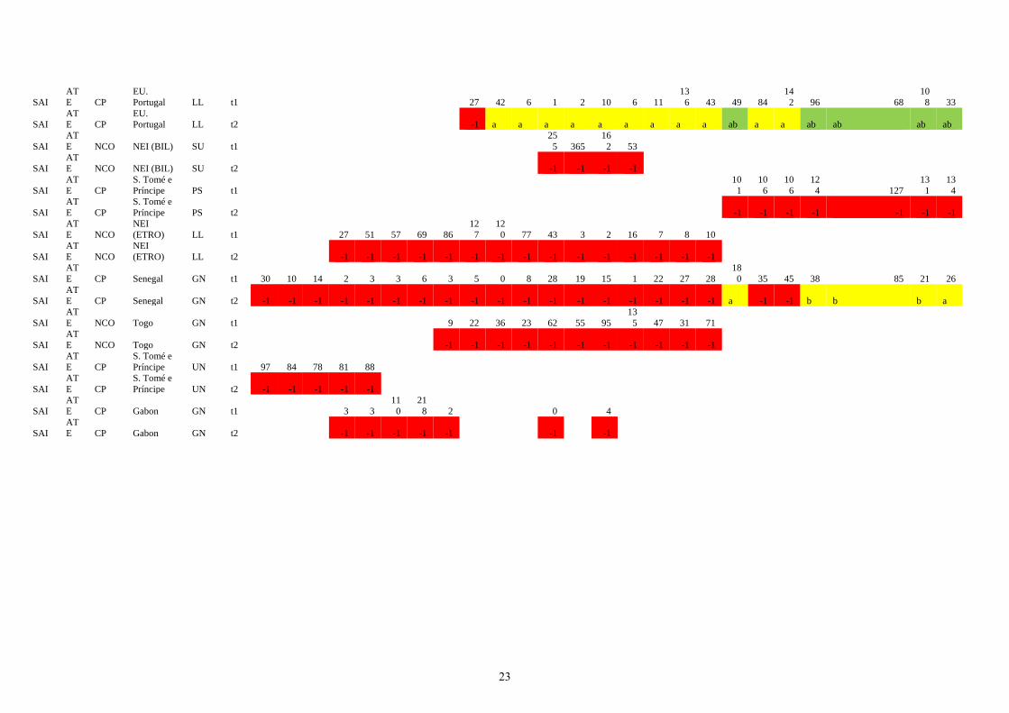
SAI

AT

E CP

EU.

Portugal LL t1

27 42 6 1 2 10 6 11

13

6 43 49 84

14

2 96 68

10

8 33

SAI

AT

E CP

EU.

Portugal LL t2

-1 a a a a a a a a a ab a a ab ab ab ab

SAI

AT

E NCO NEI (BIL) SU t1

25

5 365

16

2 53

SAI

AT

E NCO NEI (BIL) SU t2

-1 -1 -1 -1

SAI

AT

E CP

S. Tomé e

Príncipe PS t1

10

1

10

6

10

6

12

4 127

13

1

13

4

SAI

AT

E CP

S. Tomé e

Príncipe PS t2

-1 -1 -1 -1 -1 -1 -1

SAI

AT

E NCO

NEI

(ETRO) LL t1

27 51 57 69 86

12

7

12

0 77 43 3 2 16 7 8 10

SAI

AT

E NCO

NEI

(ETRO) LL t2

-1 -1 -1 -1 -1 -1 -1 -1 -1 -1 -1 -1 -1 -1 -1

SAI

AT

E CP Senegal GN t1 30 10 14 2 3 3 6 3 5 0 8 28 19 15 1 22 27 28

18

0 35 45 38 85 21 26

SAI

AT

E CP Senegal GN t2 -1 -1 -1 -1 -1 -1 -1 -1 -1 -1 -1 -1 -1 -1 -1 -1 -1 -1 a -1 -1 b b b a

SAI

AT

E NCO Togo GN t1

9 22 36 23 62 55 95

13

5 47 31 71

SAI

AT

E NCO Togo GN t2

-1 -1 -1 -1 -1 -1 -1 -1 -1 -1 -1

SAI

AT

E CP

S. Tomé e

Príncipe UN t1 97 84 78 81 88

SAI

AT

E CP

S. Tomé e

Príncipe UN t2 -1 -1 -1 -1 -1

SAI

AT

E CP Gabon GN t1

3 3

11

0

21

8 2

0

4

SAI

AT

E CP Gabon GN t2

-1 -1 -1 -1 -1

-1

-1

23

Table 6. Tag releases and recaptures by year in the ICCAT tagging database.

Years at liberty

Year Releases Recaptures < 1 1 - 2 2 - 3 3 - 4 4 - 5 5 - 10 10+ 15+ ERROR % recapt*

1950 2 1

1

50.0%

1951 1 1 1

100.0%

1952 2 2 2

100.0%

1953 1 1

1

100.0%

1954 3 0

1955 13 2

2

15.4%

1956 2 1

1

50.0%

1957 59 2 1 1

3.4%

1958 31 2 1 1

6.5%

1959 252 1

1

0.4%

1960 926 5 3 2

0.5%

1961 1303 7 5 2

0.5%

1962 1497 10 7 3

0.7%

1963 1423 8 8

0.6%

1964 1305 6 6

0.5%

1965 1316 9 8 1

0.7%

1966 1277 17 13 2 1

1

1.3%

1967 877 13 12 1

1.5%

1968 847 10 8 2

1.2%

1969 819 7 5 1

1

0.9%

1970 632 2 1

1

0.3%

1971 1074 4 2 1 1

0.4%

1972 920 6 3 3

0.7%

1973 914 17 7 8

1

1

1.9%

1974 870 10 4 4 2

1.1%

1975 1017 17 14 3

1.7%

1976 1464 22 15 7

1.5%

1977 1391 32 24 4 1 2

1

2.3%

1978 1549 32 18 11 2

1

2.1%

1979 1860 37 23 4 5 2 1

2

2.0%

1980 2125 49 24 9 2 1 1

11 1

2.3%

1981 1853 43 34 4 4 1

2.3%

1982 1643 32 20 7 2 2 1

1.9%

1983 1824 13 8 4 1

0.7%

1984 2212 32 16 7 4 2 1 2

1.4%

1985 1912 41 26 8 3

2 2

2.1%

1986 2238 44 32 8 4

2.0%

1987 1999 46 24 10 6 3

3

2.3%

1988 2487 50 30 7 4 4 2 3

2.0%

1989 2183 50 24 18 7

1

2.3%

1990 3403 85 48 23 6 6 1 1

2.5%

1991 4912 140 75 41 17 2 3 2

2.9%

1992 5878 147 87 41 13 2 1 3

2.5%

24

1993 5540 124 80 29 11

1 3

2.2%

1994 5708 93 57 16 9 7 1 3

1.6%

1995 6512 96 57 23 7 6 1 2

1.5%

1996 4933 118 63 31 17 2 3 2

2.4%

1997 5454 106 58 26 13 5 2 2

1.9%

1998 5021 106 56 30 12 5 1 1

1 2.1%

1999 7174 127 83 24 12 5 1 2

1.8%

2000 5148 54 36 9 7

2 1.0%

2001 3866 43 27 8 2 2 3

1 1.1%

2002 4186 31 21 6 1 2

1 0.7%

2003 2977 17 12 4 1

0.6%

2004 447 17 8 7 1

1 3.8%

2005 448 23 17 6

5.1%

2006 8 8 7

1 100.0%

2011 5 1 1

20.0%

Grand Total 115743 2020 1222 471 181 63 28 32 13 3 7 1.7%

25

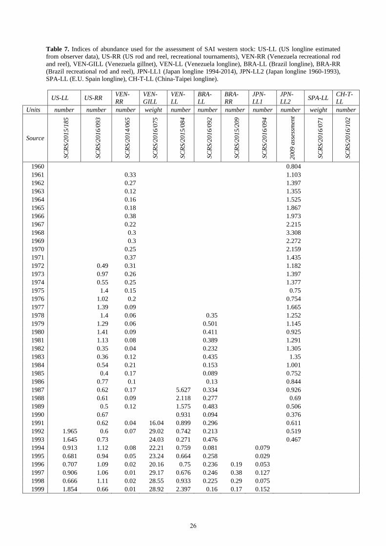
Table 7. Indices of abundance used for the assessment of SAI western stock: US-LL (US longline estimated

from observer data), US-RR (US rod and reel, recreational tournaments), VEN-RR (Venezuela recreational rod

and reel), VEN-GILL (Venezuela gillnet), VEN-LL (Venezuela longline), BRA-LL (Brazil longline), BRA-RR

(Brazil recreational rod and reel), JPN-LL1 (Japan longline 1994-2014), JPN-LL2 (Japan longline 1960-1993),

SPA-LL (E.U. Spain longline), CH-T-LL (China-Taipei longline).

US-LL US-RR VEN-

RR

VEN-

GILL

VEN-

LL

BRA-

LL

BRA-

RR

JPN-

LL1

JPN-

LL2 SPA-LL

CH-T-

LL

Units number number number weight number number number number number weight number

Source

SC

RS

/20

15

/18

5

SC

RS

/20

16

/09

3

SC

RS

/20

14

/06

5

SC

RS

/20

16

/07

5

SC

RS

/20

15

/08

4

SC

RS

/20

16

/09

2

SC

RS

/20

15

/20

9

SC

RS

/20

16

/09

4

20

09

ass

essm

ent

SC

RS

/20

16

/07

1

SC

RS

/20

16

/10

2

1960

0.804

1961

0.33

1.103

1962

0.27

1.397

1963

0.12

1.355

1964

0.16

1.525

1965

0.18

1.867

1966

0.38

1.973

1967

0.22

2.215

1968

0.3

3.308

1969

0.3

2.272

1970

0.25

2.159

1971

0.37

1.435

1972

0.49 0.31

1.182

1973

0.97 0.26

1.397

1974

0.55 0.25

1.377

1975

1.4 0.15

0.75

1976

1.02 0.2

0.754

1977

1.39 0.09

1.665

1978

1.4 0.06

0.35

1.252

1979

1.29 0.06

0.501

1.145

1980

1.41 0.09

0.411

0.925

1981

1.13 0.08

0.389

1.291

1982

0.35 0.04

0.232

1.305

1983

0.36 0.12

0.435

1.35

1984

0.54 0.21

0.153

1.001

1985

0.4 0.17

0.089

0.752

1986

0.77 0.1

0.13

0.844

1987

0.62 0.17

5.627 0.334

0.926

1988

0.61 0.09

2.118 0.277

0.69

1989

0.5 0.12

1.575 0.483

0.506

1990

0.67

0.931 0.094

0.376

1991

0.62 0.04 16.04 0.899 0.296

0.611

1992 1.965 0.6 0.07 29.02 0.742 0.213

0.519

1993 1.645 0.73

24.03 0.271 0.476

0.467

1994 0.913 1.12 0.08 22.21 0.759 0.081

0.079

1995 0.681 0.94 0.05 23.24 0.664 0.258

0.029

1996 0.707 1.09 0.02 20.16 0.75 0.236 0.19 0.053

1997 0.906 1.06 0.01 29.17 0.676 0.246 0.38 0.127

1998 0.666 1.11 0.02 28.55 0.933 0.225 0.29 0.075

1999 1.854 0.66 0.01 28.92 2.397 0.16 0.17 0.152

26

2000 2.689 0.61 0.06 23.83 0.693 0.218 0.45 0.094

2001 1.002 0.74 0.06 22.42 0.431 0.304 0.23 0.017

0.61356

2002 0.661 0.83

20.51 0.507 0.154 0.26 0.047

0.78549

2003 0.456 0.94

19.74 0.314 0.241 0.42 0.098

0.68082

2004 0.791 0.99

21.12 0.347 0.213 0.29 0.046

0.35385

2005 1.011 0.97

25.17 0.405 0.443 0.43 0.118

0.66841

2006 0.521 1.14

28.43 0.726 0.186 0.58 0.082

0.62019

2007 0.608 0.97

31.02 1.84 0.152 0.62 0.017

0.81285

2008 1.105 1.57

31.75 0.462 0.077 0.46 0.227

1.18685

2009 0.796 1.74

32.35 0.526 0.271 0.02 0.223

1.40152 0.054

2010 0.877 1.79

31.56 0.511 0.05 0.16 0.213

1.39395 0.083

2011 0.768 2.03

37.75 0.724 0.179 0.11 0.272

1.238 0.068

2012 1.087 2.08

36.13 0.946 0.033 0.14 0.122

1.22106 0.086

2013 0.631 1.45

37.8 0.784

0.19 0.105

1.86786 0.058

2014 0.658 1.33

40.24 0.442

0.07 0.234

1.15559 0.027

27

Table 8. Indices of abundance used for the assessment of SAI eastern stock: CIV-ART (Cote d’Ivoire artisanal),

SEN-ART (Senegal artisanal), GHA-ART (Ghana artisanal), JPN-LL1 (Japan longline 1994-2014), JPN-LL2

(Japan longline 1960-1993), SPA-LL (E.U. Spain longline), CH-T-LL (China-Taipei longline), POR-LL (E.U.

Portugal longline).

CIV-ART SEN-

ART GHA-ART JPN-LL1 JPN-LL2

SPA-LL CH-T-LL POR-LL

Units number weight weight number number weight number weight

Source

Ko

nan

et

al.

20

10

SC

RS

/P/2

01

6/0

26

SC

RS

/P/2

01

6/0

27

SC

RS

/20

16

/09

4

no

cu

rren

t p

ap

er

SC

RS

/20

16

/07

1

SC

RS

/20

16

/10

2

SC

RS

/20

16

/09

8

1960

0.736

1961

5.036

1962

1.080

1963

0.778

1964

2.405

1965

2.028

1966

1.951

1967

0.660

1968

1.799

1969

2.846

1970

4.269

1971

1.086

1972

1.007

1973

0.579

1974

0.211895562

0.470

1975

0.861368814

0.449

1976

0.957747662

0.612

1977

0.112948668

0.375

1978

0.163621417

0.686

1979

0.212812227

0.262

1980

0.180083326

0.527

1981

0.748 0.086482684

0.325

1982

1.104 0.935583116

1.078

1983

0.695

0.421

1984

0.480 0.201801942

1.147

1985

0.975 0.175561492

0.635

1986

1.127 0.509489735

0.670

1987

1.526 0.262844857

0.485

1988 0.610 1.268 4.668112227

0.483

1989 0.300 1.904 0.028988173

0.398

1990 0.350 1.479 1.526036311

0.250

1991 0.400 1.491 3.314307472

0.198

1992 0.180 1.293 1.931277986

0.212

1993 0.180 0.780 1.863091017

0.379

1994 0.240 0.335 1.626846167 0.046

1995 0.120 0.612 0.775487009 0.048

1996 0.110 1.263 2.386733581 0.040

1997 0.190 1.892 1.294619842 0.028

1998 0.160 1.244 0.823348625 0.038

1999 0.250 0.951 0.564210346 0.029

3.980

28

2000 0.110 1.133 0.36950505 0.037

1.520

2001 0.180 1.847 0.93782419 0.013

0.136

1.400

2002 0.200 1.448 1.756970257 0.029

0.725

2.120

2003 0.100 2.116 2.219196392 0.035

0.483

0.740

2004 0.200 0.692 0.818136506 0.072

0.471

1.280

2005 0.200 0.811 1.327515512 0.078

0.574

1.180

2006 0.200 0.523 0.70223582 0.062

0.672

0.410

2007 0.250 0.609 0.645313986 0.094

0.812

0.470

2008

0.741 0.611763543 0.115

1.066

0.290

2009

0.556 1.526725834 0.071

1.187 0.054 0.370

2010

0.382

0.073

0.874 0.050 0.080

2011

0.296 0.496332575 0.122

0.773 0.056 0.900

2012

0.412 0.712631818 0.104

1.408 0.078 0.830

2013

0.269 0.200548261 0.114

2.339 0.090 0.710

2014

0.076

2.480 0.056 1.770

Table 9. Bayesian production model runs in the East.

Number Index trend Weighting Software

Process

error Bo/K

r prior

mean converged

1a up equal BSP-VB 0 prior 0.54 yes

1b up catch BSP-VB 0 prior 0.54 yes

1c up by series BSP-VB 0 prior 0.54 no

2a down equal BSP-VB 0 prior 0.54 yes

2b down catch BSP-VB 0 prior 0.54 yes

2c down by series BSP-VB 0 prior 0.54 no

1a up equal JAGS 0.05 prior 0.54 yes

1b up catch JAGS 0.05 prior 0.54 yes

1c up by series JAGS 0.05 prior 0.54 yes

2a down equal JAGS 0.05 prior 0.54 yes

2b down catch JAGS 0.05 prior 0.54 yes

2c down by series JAGS 0.05 prior 0.54 yes

3a down, 2 GHN equal JAGS 0.05 prior 0.54 yes

3b down, GHN 92+ equal JAGS 0.05 prior 0.54 yes

1d up equal JAGS 0.05 prior 0.3 yes

2d down equal JAGS 0.05 prior 0.3 yes

1e up equal JAGS 0.05 fixed=1 0.54 yes

2e down equal JAGS 0.05 fixed=1 0.54 yes

1f up equal JAGS 1E-06 prior 0.54 yes

1g up equal JAGS 0 prior 0.54 no

29

Table 10. Means and CVs of parameters from BSP-JAGS models in the east.

Model

K

(1000) r Bo/K MSY (1000)

Bcur/

Bmsy

HRcur/

HRmsy

E-up-equal wt

23.41

(0.96) 1.23 (0.22)

0.45

(1.1)

6.8

(0.75) 0.67 (0.43)

0.33

(0.33)

E-up-catch wt.

66.35

(1.18) 0.59 (0.31) 0.45 (1.57)

8.98

(1.1)

0.4

(2.07)

2.85

(2.44)

E-up-series wt.

27.04

(0.48) 1.17 (0.22) 0.45 (1.12)

7.67

(0.41) 0.41 (0.38)

0.45

(0.29)

E-down-equal wt.

15.7

(0.77) 1.39 (0.24) 0.44 (1.07)

5.08

(0.57) 0.71 (0.86)

0.61

(0.81)

E-down-catch wt.

71.94

(1.27) 0.59 (0.31) 0.43 (1.56)

9.6

(1.16) 0.36 (1.61)

2.85

(2.51)

E-down-series wt.

18.94

(0.5) 1.28 (0.22) 0.46 (1.08)

5.79

(0.42) 0.32 (0.94)

1.35

(1.19)

E-down-equal-2

GHN

24.23

(2.99)

1.6

(0.2)

0.40

(1.13)

8.58

(2.36) 0.41 (0.62)

0.61

(0.52)

E-down-equal-

GHN 92+

20.94

(1.58) 1.42 (0.21)

0.42

(1.1)

7.03

(1.21) 0.41 (0.62)

0.62

(0.55)

E-up-prior.3

91.08

(2.14)

0.7

(0.27) 0.56 (1.17) 13.48 (2.01) 0.52 (0.59)

0.51

(0.37)

E-down-prior.3

62.43

(2.22) 0.63 (0.28) 0.61 (1.15)

8.58

(2.08) 0.14 (2.46)

63.97

(3.23)

E-up-Bo=K

21.68

(0.37) 1.22 (0.22) 1

6.4

(0.33)

0.66

(0.4)

0.34

(0.33)

E-down-B0=K

17.25

(0.82) 1.21 (0.25) 1

4.83

(0.6) 0.29 (2.16)

38.58

(3.74)

E-up-low process

22.73

(0.62) 1.22 (0.22)

0.46

(1.1)

6.65

(0.49) 0.66 (0.42)

0.34

(0.33)

Table 11. Results for sailfish eastern Atlantic with varying catch scenarios, indices used, separation of Ghana

series (Ghana1 and Ghana2), and omission of 1988-1990 from Ghana index.

30

Table 12. Bootstrap results for ASPIC runs for ASPIC Run E1 with CPUE Indices Exhibiting a Negative Trend.

Parameter Estimate

80%

lower

80%

upper

50%

lower

50%

upper

Interquartile

range

Relative

IQ Range

B1/K 1.00 NA NA NA NA NA NA

MSY 1657.00 1152.00 1951.00 1448.00 1855.00 406.80 0.25

Fmsy 0.08 0.03 0.13 0.06 0.11 0.05 0.70

Ye(2015) 780.30 518.10 1260.00 685.10 1040.00 354.50 0.45

Y.(Fmsy) 464.60 291.50 849.70 388.50 655.00 266.50 0.57

Bmsy

21480.0

0 14900.00 33580.00 16800.00 26150.00 9343.00 0.44

B./Bmsy 0.27 0.16 0.43 0.21 0.34 0.14 0.51

F./Fmsy 2.55 1.41 3.92 1.86 3.00 1.15 0.45

Ye./MSY 0.47 0.30 0.68 0.37 0.57 0.20 0.43

Table 13. Key parameters associated with the stock production analysis for SAI_west.

Parameter Lower 80% CI Geometric Mean Upper 80% CI

r 0.18 0.35 0.67

K 10233 15250 25592

MSY 1130 1317 1534

BMSY 18727 36470 71025

B2014/BMSY * 0.23 0.42 0.61

F2014/FMSY * 0.69 1.37 2.45

*Based on Shaefer models

Table 14. Key parameters associated with the stock production analysis for SAI_east.

Parameter Lower 80% CI Geometric Mean Upper 80% CI

r 0.194 0.263 0.356

K 18727 36470 71025

MSY 1812 1977 2157

BMSY 9363 18235 35513

B2014/BMSY * 0.22 0.49 0.70

F2014/FMSY * 0.16 0.96 2.42

*median est (other pars Gem. Mean)

31

Figure 1. Spatial distribution of sailfish mitochondrial DNA sampling.

Figure 2. Sailfish abundance indices predicted from the fitted delta generalized additive models for Jan. – Mar.

(a), Apr. – Jun. (b), Jul. – Sep. (c), and Oct. – Dec. (d). Predictions were generated from data fishnets (0.1° latitude

by 0.1° longitude) representing seasonal averages of numerical model descriptors for the year 2010. Fishnets were

generated using data from NCEI and NOAA. Plots were generated from the daytime fishnets (nighttime fishnets

displayed similar patterns with slightly larger abundance indices).

32

0

50

100

150

200

250

0 2 4 6 8 10 12

Lo

we

r-J

aw

Fo

rkle

ng

th (

CM

)

Age

Cerdenares-Ladrón De Guevara et al., 2011

Fitchett and Ehrhardt, 2016 (Dissertation)

Hedgepeth and Jolley 1983 Female

Hedgepeth and Jolley 1983 Male

Alvarado-Castillo and Felix-Uraga, 1998

Freire et al, 1999

Ehrhardt and Deleveaux 2006 Female

Ehrhardt and Deleveaux 2006 Male

Figure 3. Von Bertalanffy growth plots examined to determine appropriate sailfish growth parameters to be used

in assessment.

Figure 4. Sailfish Task I nominal catches (t) by year for western (red line) and eastern stock (blue line).

0

1000

2000

3000

4000

5000

6000

19

50

19

53

19

56

19

59

19

62

19

65

19

68

19

71

19

74

19

77

19

80

19

83

19

86

19

89

19

92

19

95

19

98

20

01

20

04

20

07

20

10

20

13

ATE

ATW

33

Figure 5. Straight displacements between release and recovery positions (apparent movement), from conventional

tagging of sailfish.

Figure 6. Density (5 by 5 degrees squares) of SAI releases (left) and recoveries (right).

34

Figure 7. Indices of abundance used for the western sailfish stock.

Figure 8. Indices of abundance used for the eastern sailfish stock.

35

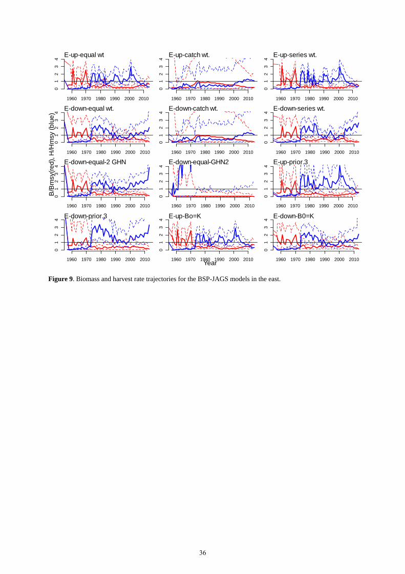
Figure 9. Biomass and harvest rate trajectories for the BSP-JAGS models in the east.

1960 1970 1980 1990 2000 2010

01

23

4E-up-equal wt

1960 1970 1980 1990 2000 2010

01

23

4

E-up-catch wt.

1960 1970 1980 1990 2000 2010

01

23

4

E-up-series wt.

1960 1970 1980 1990 2000 2010

01

23

4

E-down-equal wt.

1960 1970 1980 1990 2000 2010

01

23

4

E-down-catch wt.

1960 1970 1980 1990 2000 2010

01

23

4

E-down-series wt.

1960 1970 1980 1990 2000 2010

01

23

4

E-down-equal-2 GHN

1960 1970 1980 1990 2000 2010

01

23

4E-down-equal-GHN2

1960 1970 1980 1990 2000 2010

01

23

4

E-up-prior.3

1960 1970 1980 1990 2000 2010

01

23

4

E-down-prior.3

1960 1970 1980 1990 2000 2010

01

23

4

E-up-Bo=K

1960 1970 1980 1990 2000 2010

01

23

4

E-down-B0=K

B/B

msy(r

ed

), H

/Hm

sy (

blu

e)

Year

36

Figure 10. Retrospective Analyses for ASPIC run E1 for F/FMSY (upper panel) and B/BMSY (lower panel).

37

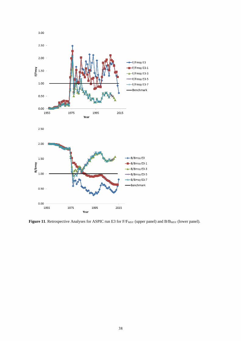
Figure 11. Retrospective Analyses for ASPIC run E3 for F/FMSY (upper panel) and B/BMSY (lower panel).

38

Figure 12. Prior on FMSY for ASPIC surplus production model of western Atlantic sailfish.

Beta prior on Fmsy

Fmsy

De

nsity

0.0 0.2 0.4 0.6

01

23

39

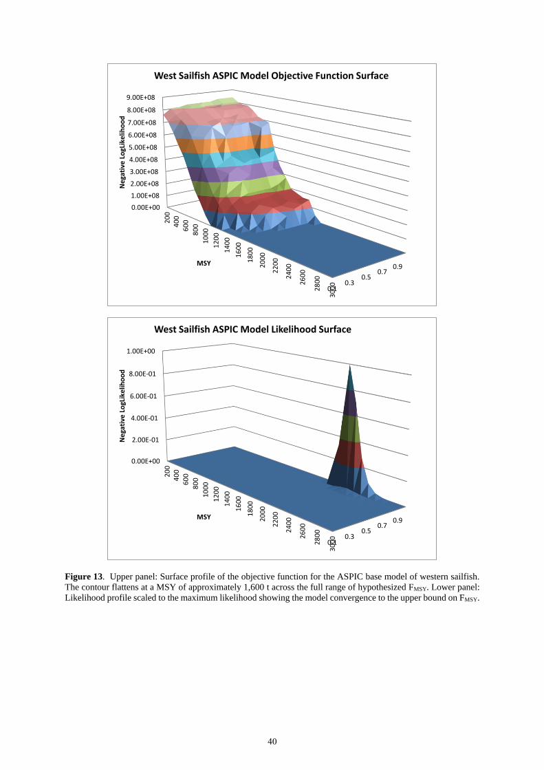
Figure 13. Upper panel: Surface profile of the objective function for the ASPIC base model of western sailfish.

The contour flattens at a MSY of approximately 1,600 t across the full range of hypothesized FMSY. Lower panel:

Likelihood profile scaled to the maximum likelihood showing the model convergence to the upper bound on FMSY.

0.10.3

0.50.7

0.9

0.00E+00

1.00E+08

2.00E+08

3.00E+08

4.00E+08

5.00E+08

6.00E+08

7.00E+08

8.00E+08

9.00E+08

20

04

00

60

0

80

0

10

00

12

00

14

00

16

00

18

00

20

00

22

00

24

00

26

00

28

00

30

00

Ne

gati

ve L

ogL

ike

liho

od

MSY

West Sailfish ASPIC Model Objective Function Surface

0.10.3

0.50.7

0.9

0.00E+00

2.00E-01

4.00E-01

6.00E-01

8.00E-01

1.00E+00

20

04

00

60

0

80

0

10

00

12

00

14

00

16

00

18

00

20

00

22

00

24

00

26

00

28

00

30

00

Ne

gati

ve L

ogL

ike

liho

od

MSY

West Sailfish ASPIC Model Likelihood Surface

40

Figure 14. Bootstrap estimates of FMSY from the ASPIC base model for western sailfish. The distribution of

estimates is spread across the lower (0.01) and upper bounds (0.8) defined in the model.

Figure 15. Fit to indices of abundance used in each of Model_1 (left) and Model_2 (right).

Fmsy Bootstrap Estimates

Fmsy

Fre

qu

en

cy

0.0 0.1 0.2 0.3 0.4 0.5 0.6 0.7

05

10

15

20

25

30

41

Figure 16. Observed (bars) and expected (blue line) mean weight of catch from the three gear types for Model_1

(left) and Model_2 (right).

42

Figure 17. Overall fit to length composition data from each of the three gear types for Model_1 (top) and Model_2

(bottom).

43

Figure 18. Estimated historic trends in spawning stock biomass (upper left), recruitment (upper right), F/FMSY

(lower left) and B/BMSY (lower right) for Model_1 (blue) and Model_2 (red).

44

Figure 19. Retrospective analysis Model_1 (top) and Model_2 (bottom).

45

Figure 20. Estimated historic trends in spawning stock biomass (upper left), recruitment (upper right), F/FMSY

(lower left) and B/BMSY (lower right) for Model_1 (dark blue) and Model_2 (dark red), Model_1.1 (light blue) and

Model_2.1 (light red).

Figure 21. Retrospective analysis for Model_2.1.

46

Figure 22. Prior, maximum likelihood, and posterior distributions from MCMC analysis of Model_1.1. Red

triangle represents the starting value and the dotted line the posterior median value.

47

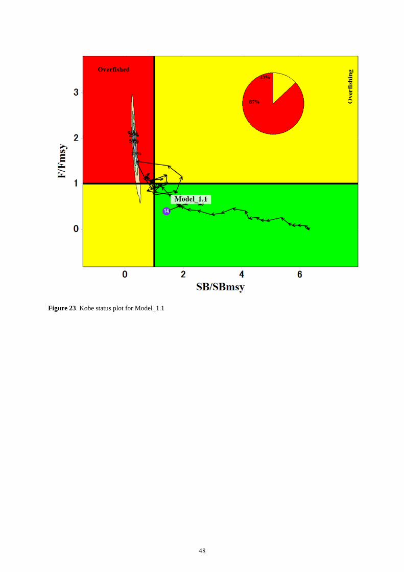
Figure 23. Kobe status plot for Model_1.1

48

Figure 24. Prior, maximum likelihood, and posterior distributions from MCMC analysis of Model_2.1. Red

triangle represents the starting value and the dotted line the posterior median value.

49

Figure 25. Kobe status plot for Model_2.1

Figure 26. Posterior distributions of r, K, and MSY for SRA SAI_west.

50

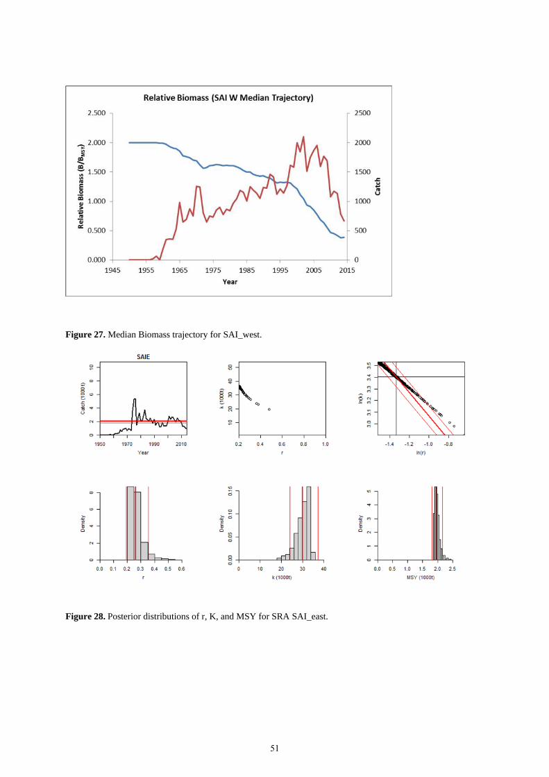
Figure 27. Median Biomass trajectory for SAI_west.

Figure 28. Posterior distributions of r, K, and MSY for SRA SAI_east.

51

Figure 29. Median Biomass trajectory for SAI_east.

52

Appendix 1

Agenda

1. Opening, adoption of the Agenda and meeting arrangements.

2. Summary of available data for assessment

2.1. Biology

2.2. Catch, effort, and size

2.3. Relative abundance estimates (CPUEs)

3. Stock Assessment

3.1. SAI east

3.2. SAI west

4. Management recommendations

4.1. SAI east

4.2. SAI west

5. Recommendations on research and statistics

6. Other matters

7. Adoption of the report and closure

53

Appendix 2

List of Participants

BRAZIL

Leite Mourato, Bruno Profesor Adjunto, Departamento de Ciências do Mar, Universidade Federal de São Paulo Avenida Almirante Saldanha da

Gama, 89. Ponta da Praia, 11030-400 Santos, SP, Brazil

Tel: +55 61 2023 3540, Fax: +55 61 2023 3909, E-Mail: [email protected];[email protected]

CÔTE D'IVOIRE

Konan, Kouadio Justin Chercheur Hidrobiologiste, Centre de Recherches Océanologiques (CRO), 29 Rue des Pêcheurs, BP V 18, Abidjan 01, Côte

d'Ivoire

Tel: +225 07 625 271, Fax: +225 21 351155, E-Mail: [email protected]

EUROPEAN UNION

Fernández Costa, Jose Ramón Ministerio de Economía y Competitividad, Instituto Español de Oceanografía - C. Costero de A Coruña, Paseo Marítimo

Alcalde Francisco Vázquez, 10 - P.O. Box 130, 15001 A Coruña, Spain

Tel: +34 981 218 151, Fax: +34 981 229 077, E-Mail: [email protected]

GHANA

Ayivi, Sylvia Sefakor Awo Fisheries Directorate of the Ministry of Food and Agriculture, Marine Fisheries Research Division P.O. Box BT 62, Tema,

Ghana

Tel: + 233 2441 76300, Fax: +233 3032 008048, E-Mail: [email protected]

S. TOMÉ E PRÍNCIPE

Da Conceiçao, Ilair Chef du Département de Recherche, Statistiques et de l'aquaculture, Direcçao das Pescas, Responsavel pelo serviço de

Estatística Pesqueira Bairro 3 de Fevereiro - PB 59, Sao Tomé, São Tomé and Príncipe

Tel: +239 990 9315, Fax: +239 12 22 414, E-Mail: [email protected]

SENEGAL

Sow, Fambaye Ngom Chercheur Biologiste des Pêches, Centre de Recherches Océanographiques de Dakar Thiaroye, CRODT/ISRALNERV - Route

du Front de Terre - BP 2241, Dakar, Senegal

Tel: +221 3 0108 1104; +221 77 502 67 79, Fax: +221 33 832 8262, E-Mail: [email protected]

UNITED STATES

Babcock, Elizabeth Rosenstiel School of Marine and Atmospheric Science, University of Miami, 4600 Rickenbacker Causeway, Miami, Florida

33133, United States


Brown, Craig A. Chief, Highly Migratory Species Branch, Sustainable Fisheries Division, NOAA Fisheries Southeast Fisheries Science Center,

75 Virginia Beach Drive, Miami Florida 33149, United States


Díaz, Guillermo NOAA-Fisheries, Southeast Fisheries Science Center, 75 Virginia Beach Drive, Miami Florida 33139, United States

Tel: +1 305 361 4277, E-Mail: [email protected]

Die, David SCRS Chairman, Cooperative Institute of Marine and Atmospheric Studies, University of Miami, 4600 Rickenbacker

Causeway, Miami Florida 33149, United States


54

mailto:[email protected]



Fitchett, Mark University of RSMAS, 4600 Rickenbacker Causeway, Miami Florida 33149, United States Tel: +1 305 989 8308, Fax: +1 305 421 4600, E-Mail: [email protected]

Forrestal, Francesca Cooperative Institute of Marine and Atmospheric Studies, University of Miami, RSMAS/CIMAS4600 Rickenbacker Causeway, Miami Florida 33149, United States


Hoolihan, John

NOAA Fisheries, Southeast Fisheries Science Center75 Virginia Beach Drive, Miami Florida 33149, United States


Lauretta, Matthew

NOAA Fisheries Southeast Fisheries Center, 75 Virginia Beach Drive, Miami, Florida 33149, United States


Perryman, Holly

CSWY, 4600 Rickenbacker CSWY, Miami, FL 33165, United States


Prince, Eric

33 Senner Court, Shalimar Florida 32579, United States


Schirripa, Michael

NOAA Fisheries, Southeast Fisheries Science Center75 Virginia Beach Drive, Miami Florida 33149, United States


Sharma, Rishi

SEFSC, 75 Virginia Beach Drive, Miami, Florida 33149, United States


Walter, John

NOAA Fisheries, Southeast Fisheries Center, Sustainable Fisheries Division75 Virginia Beach Drive, Miami, Florida 33149,

United States

Tel: +305 365 4114, Fax: +1 305 361 4562, E-Mail: [email protected]

VENEZUELA

Arocha, Freddy Instituto Oceanográfico de Venezuela Universidad de Oriente, A.P. 204, 6101 Cumaná Estado Sucre, Venezuela Tel: +58-293-400-2111 ; mobile +58 416 693 0389, E-Mail: [email protected]; [email protected]

OBSERVERS FROM COOPERATING NON-CONTRACTING PARTIES, ENTITIES, FISHING ENTITIES

CHINESE TAIPEI

Su, Nan-Jay

Assistant Professor, Department of Environmental Biology and Fisheries Science, No. 2 Pei-Ning Rd. Keelung, Taiwan,

Chinese Taipei

Tel: +886 2 2462-2192 #5046, E-Mail: [email protected]

OBSERVERS FROM INTERGOVERNMENTAL ORGANIZATIONS

FOOD AND AGRICULTURE ORGANIZATION - FAO

Pérez Moreno, Manuel

United Nations House, Christ Church, BB11000 Bridgetown, Barbados


ICCAT De Bruyn, Paul ICCAT Secretariat,

Mail: [email protected]

55







Appendix 3

List of documents

SCRS/2016/071

Standardized catch rates of sailfish (Istiophorus albicans)

caught as bycatch of the Spanish surface longline fishery

targeting swordfish (Xiphias gladius) in the Atlantic

Ocean

García-Cortés B., Ramos-Cartelle A.,

Fernández-Costa J., and Mejuto J.

SCRS/2016/075

Standardized CPUE from the Rod and Reel and artisanal

drift-gillnet fisheries off La Guaira, Venezuela, updated

through 2014.

Babcock E.A., and Arocha F.

SCRS/2016/092

Standardized catch rates of sailfish caught by the Brazilian

fleet (1978-2012) using a Generalized Linear Mixed Model

(GLMM), with a delta log approach

Mourato B.L., Hazin H., Carvalho F.,

and Hazin F.

SCRS/2016/093

Estimated sailfish catch-per-unit-effort for the U.S.

recreational billfish tournaments and U.S. recreational

fishery (1972-2014)

Hoolihan J.P., and Lauretta M.

SCRS/2016/094

Standardized CPUE for sailfish caught by the Japanese

tuna longline fishery in the Atlantic Ocean from 1994 to

2014

Kai M., and Okamoto H.

SCRS/2016/095 Regional Caribbean Billfish Management and

Conservation Plan Perez-Moreno M.

SCRS/2016/098

Characterization and standardization of the Atlantic

sailfish (Istiophorus albicans) catch rates in the East

Atlantic from the Portuguese pelagic longline fishery

Coelho R., Lino P.G., and Santos

M.N.

SCRS/2016/099

Generalized additive models for predicting the spatial

distribution of billfishes and tunas across the Gulf of

Mexico

Perryman H.A., and Babcock E.A.

SCRS/2016/100 An assessment of Western Atlantic sailfish for 2016 Schirripa M.J.

SCRS/2016/101 Maximum sizes in the Atlantic sailfish catch Goodyear C.P., and Schirripa M.J.

SCRS/2016/102

CPUE standardization of sailfish (Istiophorus platypterus)

for the Taiwanese distant-water longline fishery in the

Atlantic Ocean

Su, N-J and Sun, C-L

SCRS/2016/103

Stock Assessment of Western Atlantic Sailfish

(Istiophorus platypterus) Using a Bayesian State-Space

Surplus Production Model

Mourato, B. L. and Carvalho, F.

Presentations

SCRS/P/2016/025 Genetic stock delimitation of sailfish (Istiophorus

platypterus) in the Atlantic Ocean

Ferrette B.P.L.S., Mourato B.,

Coelho R., Santos M.N., Oliveira

C., Foresti F., Amorim A.F.,

Arocha F., Hoolihan J.,

Constance D., Ngom-Sow F.,

Mendonça F.

SCRS/P/2016/026

Relative Abundance Indices for Atlantic Sailfish

(Istiophorus albicans) from the Artisanal Fleet from

Senegal

Ngom-Sow, F. N.

SCRS/P/2016/027 Standardization of CPUE Series for the Ghanaian

Artisanal Sailfish Fishery Ayivi, S.

56

Appendix 4

Ghana data estimations

During the 2009 assessment it was reported that the catch and effort data from Ghana used in the standardization

of CPUE for the gillnet fishery had very different patterns in the relationships between CPUE, trips and number

of canoes when you compared data prior or after 1992. Such differences led the group in 2009 to disregard the

Ghana CPUE data prior to 1992. Such pattern was also seen again when the data were standardized in preparation

for the current assessment (SCRS/P/2016/027).

At the current assessment it was pointed out that the reported catch of Ghana changed greatly prior an after 1992.

Catches from the 1970s contain values five to ten times greater than those after 1992. During the mid 1970s the

Ghana catch represent more than 80% of all Atlantic catch. Such high catches prior to 1992 occurred at a time

when the number of canoes was not very different to levels post 1992, so they cannot be explained by simply the

presence of a larger fleet in the historical period (Figure 1). Furthermore, prior to 1992 the species composition

of billfish landings reported by Ghana is very different to that post 1989 (Figure 2). The post 1989 species

composition is, however, similar to the species composition of the gillnet fishery of neighboring Cote d’Ivoire

(Figure 3), except that Ghanaian catches have relatively more sailfish than Côte d’Ivoire.

All these observations suggest that the Task I reported catch of billfish for Ghana may not be accurate. The Group

recommends that Ghanaian landings prior to 1972 should be reviewed thoroughly, however, the group agreed the

reported catches from task 1 were to be used for the assessment.

The Group, however, estimated an alternative series of Ghanaian landings of billfish for the period 1956-1989 to

be used as a sensitivity analysis. Alternative catches were obtained by estimating an average species composition

of billfish for the period 1990-1999 and calculating the average catch of each billfish per canoe from the data for

that same period. The billfish catch for each year was then calculated as the product of the number of canoes that

year and the average annual catch per canoe for each species.

The alternative catch estimated for Ghana from 1973-1989 (Table 1, Figure 4) is much lower than that reported

to ICCAT in Task I but similar to catches in the 1990s, however, the catch estimated prior to 1973 is significant,

even though no catch was reported to ICCAT. It is important to note that these calculations assume that the catch

composition does not change through time, that annual catch per canoe was constant and that the number of canoes

is a good index of gillnet effort. Nunoo et al. 2015 point out that the Ghanaian fishing fleet existed long before it

started being mechanized in the 1940s, so it is possible that the catches of sailfish extend back to the 1950s and

possibly earlier.

References

Nunoo F.K.E., Asiedu B., Amador K., Blhabib D. and D. Pauly. 2015. Reconstruction of marine fisheries catches

for Ghana, 1950-2010. Fisheries Center, the University of British Columbia. Working paper Series 2015-10.

26 p.

57

Table 1. Alternative time series of billfish catch for Ghana gillnet. Catch is calculated as the product of the average

catch per canoe (1991-1999) and the number of canoes. Bold number of canoes are those reported (Nunoo et al.

2015). Other number of canoes were calculated with linear interpolation for years were there was no canoe census.

SAI BUM SWO WHM Canoes SAI BUM SWO WHM Canoes

1955 4800

1956 216 211 55 6 4940 1973 361 351 92 10 8238

1957 223 222 57 6 5080 1974 363 354 93 10 8297

1958 229 217 59 6 5220 1975 366 356 94 10 8355

1959 237 229 60 6 5360 1976 369 359 94 10 8414

1960 241 235 62 7 5500 1977 371 361 95 10 8472

1961 257 250 66 7 5859 1978 354 345 91 10 8089

1962 272 265 70 7 6217 1979 337 329 86 9 7705

1963 288 281 74 8 6576 1980 321 312 82 9 7322

1964 304 296 78 8 6935 1981 304 296 78 8 6938

1965 319 311 82 9 7293 1982 315 307 81 9 7193

1966 335 326 86 9 7652 1983 326 318 84 9 7448

1967 351 342 90 10 8011 1984 337 329 86 9 7704

1968 367 357 94 10 8369 1985 349 339 89 10 7959

1969 382 372 98 10 8728 1986 360 350 92 10 8214

1970 377 367 97 10 8606 1987 357 348 92 10 8160

1971 372 362 95 10 8483 1988 355 346 91 10 8106

1972 366 357 94 10 8361 1989 353 343 90 10 8052

58

(a) (b)

Figure 1. Canoes and landings. Ghanaian artisanal ocean-going fleet (a) Number of canoes reported by Nunoo et

al. 2015 (red dots) and lineary interpolated values (blue dots). (b) Relationship between number of canoes and

sailfish landings from task I for two periods prior to 1992 (yellow dots) and after 1991 (blackdots).

(a) (b)

Figure 2. Species composition (a) and total billfish landings (b) of task I artisanal gillnets of Ghana.

59

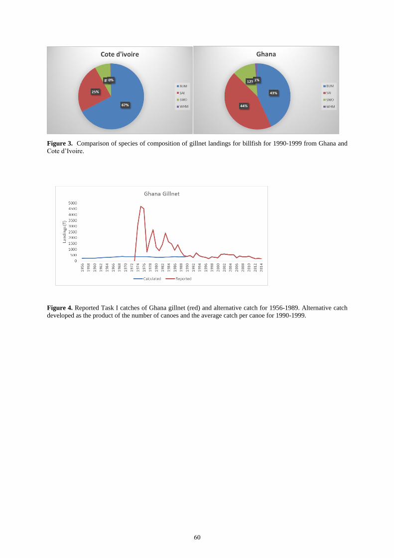
Figure 3. Comparison of species of composition of gillnet landings for billfish for 1990-1999 from Ghana and

Cote d’Ivoire.

Figure 4. Reported Task I catches of Ghana gillnet (red) and alternative catch for 1956-1989. Alternative catch

developed as the product of the number of canoes and the average catch per canoe for 1990-1999.

60

Appendix 5

Bayesian surplus production models in the East

For the eastern Atlantic population, Bayesian production models were run using both the BSP model that is

cataloged in the ICCAT catalog of methods (BSP-VB, Babcock 2007, McAllister and Babcock 2003) and a

JAGS version of the same model based on Millar and Meyer (BSP-JAGS, Meyer and Millar 1999). The JAGS

version differed from the Millar and Meyer formulation in that it included a boundary condition by which

combinations of parameter values that caused the biomass to be lower than the catch in any year were down-

weighted in the likelihood. This was implemented using the ones trick (Lunn et al. 2013). The BSP-VB model

similarly throws out parameter draws that crash the population.

The BSP-VB did not converge at all for the series weighted models, since the percent of the importance weight

on a single draw was larger than 0.5%. For the other models, the convergence diagnostics were adequate, but the

Hessian estimates of variance and covariance were not believable (Table 1). The catch weighting series put very

high weights on the Japanese longline series, and then on the Ghana series (Figure 1). The models appeared to

fit the CPUE series fairly well (Figure 2). However, the posterior distributions of both r and K were nearly

identical to the prior (Figure 3) implying that the data did not provide any information on the values of the

parameters. Because of the very wide posterior distribution of K, the population was estimated to be very large

and not heavily fished (Figure 4).

The JAGS models applied to the same datasets had much better convergence diagnostics (Table 2). Except for

the runs with catch weighting, all the runs estimated posterior distributions of r that were higher than the prior

(Figure 5). The posteriors of K were fairly well estimated.

References

Babcock, EA 2007. Application of a Bayesian surplus production model to Atlantic white marlin. Col. Vol. Sci.

Pap. ICCAT, 60(5): 1643-1651

Lunn, D., Jackson, C., Best, N., Thomas, A. and Spiegelhalter, D. 2013. The BUGS Book: A Practical

Introduction to Bayesian Analysis. CRC Press. 381 pp.

McAllister, MK and Babcock, EA. 2003. Bayesian surplus production model with the Sampling Importance

Resampling algorithm (BSP): a user’s guide. Available from www.iccat.int/en/AssessCatalog.htm

McAllister, MK, Pikitch, EK and Babcock, EA. 2001. Using demographic methods to construct Bayesian priors

for the intrinsic rate of increase in the Schaefer model and implications for stock rebuilding. Can. J. Fish.

Aquat. Sci. 58: 1871–1890.

Meyer, R. and Millar, R. B. 1999. BUGS in Bayesian stock assessments. Canadian Journal of Fisheries and

Aquatic Sciences 56(6): 1078-1087.

61

http://www.iccat.int/en/AssessCatalog.htm

Table 1. Convergence diagnostics for BSP-VP models. The percent maximum weight diagnostic should be less

than 0.5. The Hessian variance of K should be large (i.e. 1000s).

Diagnostic E-up-equal E-up-catch E-up-series E-down-equal E-down-catch E-down-series

% max wt 0.49 0.02 49.82 0.29 0.09 45.00

var(K) 3.98E-03 9.97E-07 8.80E-17 9.55E-17 5.08E-02 9.52E-17

Table 2. Convergence diagnostics for the BSP-JAGS runs in the Eastern Atlantic.

Number Description Rhat n.eff converged

1a E-up-equal wt 1.01 1800 yes

1b E-up-catch wt. 1.00 920 yes

1c E-up-series wt. 1.02 200 yes

2a E-down-equal wt. 1.12 180 yes

2b E-down-catch wt. 1.00 1300 yes

2c E-down-series wt. 1.00 990 yes

3a E-down-equal-2 GHN 1.01 1500 yes

3b E-down-equal-GHN2 302.75 2 no

1d E-up-prior.3 1.61 6 no

2d E-down-prior.3 1.15 35 yes

1e E-up-Bo=K 1.01 230 yes

2e E-down-B0=K 1.00 900 yes

1f E-up-low process 1.04 99 yes

1g E-up-no process 8.08 2 no

62

Figure 1. Catches (a), indices (b), and catch weighing (c).

Figure 2. Fit at mode of posterior distribution for the BSP-VP model for the east.

1960 1970 1980 1990 2000 2010

02000

4000

Catc

h(a)

1960 1970 1980 1990 2000 2010

01

23

4

Rela

tive C

PU

E

(b)

1960 1970 1980 1990 2000 2010

0.0

0.2

0.4

0.6

0.8

1.0

Catc

h w

eig

hts

(c)

CIVSENGHNJPN.early

JPN.lateSPNCHTPOR

1960 1970 1980 1990 2000 2010

020000

40000

60000 E-up-equal wt.

1960 1970 1980 1990 2000 2010

020000

40000

60000 E-up-catch wt.

1960 1970 1980 1990 2000 2010

020000

40000

60000

E-down-equal wt.

1960 1970 1980 1990 2000 2010

020000

60000

E-down-catch wt.

Year

Bio

ma

ss

63

Figure 3. Priors (red dashed) and posteriors (solid black) or K and r from the BSP-VP model for the East.

Figure 4. Fishing mortality (red) and biomass (blue) with 80% credible intervals.

0 1000000 2000000

0.0

0.2

0.4

0.6

0.8

K

E-up-equal wt.

0.0 0.4 0.8 1.2

0.0

00.0

20.0

40.0

60.0

80.1

00.1

2

r0 1000000 2000000

0.0

0.1

0.2

0.3

0.4

0.5

0.6

K

E-up-catch wt.

0.0 0.4 0.8 1.2

0.0

00.0

20.0

40.0

60.0

80.1

0

r

0 1000000 2000000

0.0

0.2

0.4

0.6

0.8

K

E-down-equal wt.

0.0 0.4 0.8 1.2

0.0

00.0

20.0

40.0

60.0

80.1

0

r0 1000000 2000000

0.0

0.1

0.2

0.3

0.4

0.5

0.6

0.7

K

E-down-catch wt.

0.0 0.4 0.8 1.2

0.0

00.0

20.0

40.0

60.0

80.1

0

r

Pro

ba

bility

1960 1970 1980 1990 2000 2010

0.0

0.5

1.0

1.5

2.0

E-up-equal wt.

1960 1970 1980 1990 2000 2010

0.0

0.5

1.0

1.5

2.0

E-up-catch wt.

1960 1970 1980 1990 2000 2010

0.0

0.5

1.0

1.5

2.0

E-down-equal wt.

1960 1970 1980 1990 2000 2010

0.0

0.5

1.0

1.5

2.0

E-down-catch wt.

Year

B/B

msy (

red

) a

nd

F/F

msy (

blu

e)

64

Figure 5. Priors (dashed red) and posteriors (solid black) for K and r from the BSP-JAGS models in the East.

0 50000 150000

0e+00

K

E-up-equal wt

0.0 0.5 1.0 1.5 2.0

0.0

r

0 50000 150000

0.0

e+00

K

E-up-catch wt.

0.0 0.5 1.0 1.5 2.0

0.0

r

0 50000 150000

0e+00

K

E-up-series wt.

0.0 0.5 1.0 1.5 2.0

0.0

r

0 50000 150000

0e+00

K

E-down-equal wt.

0.0 0.5 1.0 1.5 2.0

0.0

r

0 50000 1500000.0

e+00

K

E-down-catch wt.

0.0 0.5 1.0 1.5 2.0

0.0

r

0 50000 150000

0e+00

K

E-down-series wt.

0.0 0.5 1.0 1.5 2.0

0.0

r

0 50000 150000

0e+00

K

E-down-equal-2 GHN

0.0 0.5 1.0 1.5 2.0

0.0

r

0 50000 150000

0e+00

K

E-down-equal-GHN2

0.0 0.5 1.0 1.5 2.0

0.0

r

0 50000 1500000.0

e+00

K

E-up-prior.3

0.0 0.5 1.0 1.5 2.0

04

r

0 50000 1500000e+00

K

E-down-prior.3

0.0 0.5 1.0 1.5 2.0

04

r

0 50000 150000

0e+00

K

E-up-Bo=K

0.0 0.5 1.0 1.5 2.0

0.0

r

0 50000 150000

0e+00

K

E-down-B0=K

0.0 0.5 1.0 1.5 2.0

0.0

r

65

Appendix 6

Demographic estimate of r

For the Bayesian production models used in the 2009 assessment, the prior for the intrinsic rate of population

growth (r) had a mean of 0.3, implying a moderately productive stock. Carruthers and McAllister (2010) used a

demographic method to estimate a prior distribution of r, and found a mean value of 0.08, implying the

population was less production. There have been some updates to the demographic information for sailfish since

the last assessment. Therefore, the working group used the Carruthers and McAllister method with the updated

values of the biological parameters (Table 1) to produce a new demographic prior for r.

The demographic method uses estimates of the survival to each age (la), and the fecundity at each age (ma) to

calculate the population growth rate at low population sizes (r), using the Euler-Lotka equation. Assuming the

natural mortality (M) is constant, the survival to each age is calculated as exp(-Ma). Fecundity at age is

calculated from the fraction mature at age times the weight at age (calculated from length at age) times the

expected number of age 1 recruits per kg of SSB at low population size, which is calculated from steepness. The

life history parameters at age calculated from the mean values of the parameters shown in Table 1 are shown in

Figure 1.

A Monte Carlo method was used to develop a prior distribution for r. Each input parameter was given a

distribution (Table 1), with the mean agreed to be the working group, and a distribution and variance that gave a

reasonable range of values. Values of each input parameter were drawn from the specified distributions (Figure

2), and each set of parameters was used to calculate r. The resulting distribution of r values (Figure 3) is well

described by a lognormal distribution with a mean of 0.45 and CV of 0.30. This implies a much more productive

stock than was assumed in the 2009 assessment.

The Euler-Lotka method gives a value of r as an instantaneous rate. For models that use an annual time step, the

mean value of r would be exp(0.45)-1=0.57.

References

Carruthers, T. and M. McAllister. 2011. Computing prior probability distributions for the intrinsic rate of

increase for Atlantic tuna and billfish using demographic methods. Collect. Vol. Sci. Pap. ICCAT, 66(5):

2202-2205 (2011).

66

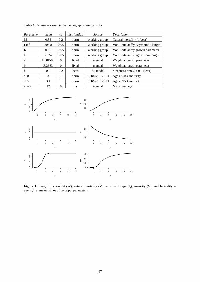
Table 1. Parameters used in the demographic analysis of r.

Parameter mean cv distribution Source Description

M 0.35 0.2 norm working group Natural mortality (1/year)

Linf 206.8 0.05 norm working group Von Bertalanffy Asymptotic length

K 0.36 0.05 norm working group Von Bertalanffy growth parameter

t0 -0.24 0.05 norm working group Von Bertalanffy age at zero length

a 1.00E-06 0 fixed manual Weight at length parameter

b 3.2683 0 fixed manual Weight at length parameter

h 0.7 0.2 beta SS model Steepness h=0.2 + 0.8 Beta()

a50 3 0.1 norm SCRS/2015/SAI Age at 50% maturity

d95 3.4 0.1 norm SCRS/2015/SAI Age at 95% maturity

amax 12 0 na manual Maximum age

Figure 1. Length (L), weight (W), natural mortality (M), survival to age (la), maturity (G), and fecundity at

age(ma), at mean values of the input parameters.

2 4 6 8 10 12

80

120

180

a

L

2 4 6 8 10 12

10

20

30

a

W

2 4 6 8 10 12

0.1

50.2

5

a

M

2 4 6 8 10 12

0.2

0.6

a

la

2 4 6 8 10 12

0.0

0.4

0.8

a

G

2 4 6 8 10 12

020

40

60

a

ma

67

Figure 2. Distributions of parameters used in the demographic analysis.

Figure 3. Histogram of r from Monte Carlo simulations. Red solid line is a lognormal distribution with the same

mean and variance, used as a prior for r.

M

M

Density

0.1 0.2 0.3 0.4 0.5 0.6

01

23

45

Linf

Linf

Density

170 190 210 230

0.0

00.0

20.0

4 K

K

Density

0.30 0.34 0.38 0.42

05

10

20

t0

t0

Density

-0.28 -0.24 -0.20

010

20

30

a

a

Density

0e+00 4e-07 8e-07

0e+00

6e+05

b

b

Density

2.0 2.5 3.0 3.5 4.0

0.0

0.2

0.4

h

h

Density

0.3 0.5 0.7 0.9

01

23

a50

a50

Density

2.0 2.5 3.0 3.5 4.0

0.0

0.4

0.8

1.2

d95

d95

Density

2.0 2.5 3.0 3.5 4.0 4.5 5.00.0

0.4

0.8

1.2

r

r

De

nsity

0.0 0.5 1.0 1.5 2.0

0.0

0.5

1.0

1.5

2.0

2.5

3.0

68

Documents

REPORT OF THE 2016 SAILFISH STOCK ASSESSMENT (Miami, …