Embed Size (px)
Citation preview

January 17, 2010
Dr. Jon Nakane,
University of British Columbia
Department of Physics and Astronomy
6224 Agricultural Road,
Vancouver, British Columbia, Canada
V6T 1Z1
Dear Dr. Nakane,
We are submitting to you our final recommendation report which follows from our APSC 479 project
work. The project goal was to optimize microwave antennas to be used in Rubidium quantum spin
manipulation experiments by Dr. Kirk Madison et al in the Quantum Degenerate Gas laboratory
(University of British Columbia, Physics Department). The designed antennas improve upon previous
prototypes by achieving greater radiation directivity and gain. The report outlines the project
background and motivation, discusses the project completion, and concludes with future design
recommendations.
Sincerely,
Taylor Dean
Engineering Physics
University of British Columbia
Dan Crawford
Engineering Physics
University of British Columbia

Microwave Antenna Design for Quantum Spin Manipulation of
Laser Cooled Rubidium Atoms
Taylor Dean
Daniel Crawford
Project Sponsor:
Dr. Kirk Madison
Quantum Degenerate Gases Laboratory
University of British Columbia
Applied Science 479
Engineering Physics
University of British Columbia
January 17, 2010
Project Number 964

i | P a g e
Executive Summary
The objective of this project is to design a set of highly directive microwave antennas: one operating
near 6.8 gigahertz and the other at 3.0 gigahertz. These antennas are to be used in a controlled
laboratory experiment to manipulate the quantum spin of laser cooled rubidium atoms. The atoms have
an associated magnetic dipole, allowing their spin to be altered with the application of resonant
microwaves.
Initially, two fabricated antenna prototypes were available: one dipole and one helix. These first
generation designs have been characterized by exploring frequency dependencies and spatial emission
patterns. It is found that the helical antenna is more directional than the dipole, and is thus chosen as
the final design type. The frequency response of the helical antenna shows a peak gain of 6.0 GHz. This
peak allows the calculation of the dielectric constant of Delrin, the core material. The physical
parameters of the helix (circumference, number of turns, length and dielectric material) are then
manipulated to guarantee that the peak intensity can be achieved at either 6.8 GHz or 3.0 GHz. The core
dielectric material of the next generation prototypes remains Delrin, since its behaviour is now well
documented and the cost is minimal.
Aside from experimental results, two methods of increasing helical antenna directionality and gain have
been researched and implemented in the final design. Four helical antennas will be placed in an array,
which leads to much higher directionality and a lower input impedance. Parasitic antennas have been
added in Helix-Helix formation around each antenna in the array. These extra elements reduce radial
radiation bleeding and direct stray wave axially.
The next generation antennas are currently under construction in the University of British Columbia
Physics and Astronomy machine shop and will be available for construction and characterization within
the first quarter of 2010.

ii | P a g e
Table of Contents Executive Summary ........................................................................................................................................ i
List of Figures ............................................................................................................................................... iii
List of Tables ................................................................................................................................................ iv
1. Background and Motivation ................................................................................................................. 1
1.1 Experiment Background ................................................................................................................ 1
1.2 Initial Prototypes ........................................................................................................................... 2
1.3 Technical Requirements ................................................................................................................ 4
1.4 Industrial Competitors – Alternative Strategies ........................................................................... 4
2. Discussion .............................................................................................................................................. 5
2.1 Project Objectives ......................................................................................................................... 5
2.2 Technical Background and Theory ................................................................................................ 6
2.2.1 Helical Antennas: Theory of Antenna Arrays and Parasitic Antennas .................................. 6
2.3 Methods and Experimental Equipment ...................................................................................... 10
2.3.1 Rubidium State Selector ...................................................................................................... 11
2.3.2 Antenna and Pick-up Antenna ............................................................................................ 13
2.3.2 Spectrum Analyzer .............................................................................................................. 14
2.4 Results ......................................................................................................................................... 15
2.4.1 Frequency Dependency ...................................................................................................... 15
2.4.2 Spatial Emission Pattern ..................................................................................................... 16
2.5 Discussion of Results ................................................................................................................... 18
2.5.1 Spatial Emission Pattern ..................................................................................................... 18
2.5.2 Frequency Dependency ...................................................................................................... 18
2.6 Final Design ................................................................................................................................. 20
2.6.1 Design Calculations ............................................................................................................. 20
2.6.2 Parasitic and Array Antennas .............................................................................................. 21
2.7 Sources of Error .......................................................................................................................... 22
3. Conclusions ............................................................................................................................................. 23
4. Recommendations .................................................................................................................................. 24
Bibliography ................................................................................................................................................ 25
Appendix A – Dimensioned Drawings ......................................................................................................... 26
Appendix B – MATLAB Script for Trace Data Compilation .......................................................................... 35

iii | P a g e
List of Figures
Figure 1 6.8GHz dipole antenna ................................................................................................................. 2
Figure 2 6.8GHz helical antenna with make-shift ground plane ................................................................ 3
Figure 3 6.8GHz helical antenna with fabricated ground plane and Delrin Shell ...................................... 3
Figure 4 The 2 by 2 Antenna Array front view (left) and side view (right) ................................................. 6
Figure 5 Helix-Helix parasitic antenna element. ........................................................................................ 8
Figure 6 Testing set-up for frequency variation and spatial distribution................................................. 10
Figure 7 Rubidium State Selector, consisting of a phase locked loop and power amplifier. ................... 11
Figure 8 Process diagram for obtaining the 6.8 GHz (top) and 3.0 GHz (bottom) signals ....................... 11
Figure 9 RbSS trace data from the spectrum analyzer for expected frequency of 6.8GHz ..................... 12
Figure 10 Two pick-up antennas used in prototype antenna characterization ......................................... 13
Figure 11 Apparatus to vary antenna and pick-up antenna radial distance and angle ............................. 13
Figure 12 Intensity vs. Frequency for the 6.8 GHz helical antenna and the 6.8 GHz dipole antenna ....... 15
Figure 13 Antenna output gain vs frequency ............................................................................................. 16
Figure 14 Top view of antenna showing sweeping method of measuring planar emission pattern ......... 16
Figure 15 Horizontal plane emission patterns ........................................................................................... 17
Figure 16 Single helical antenna with parasitic element ........................................................................... 21
Figure 17 Antenna Array Structure ............................................................................................................ 21

iv | P a g e
List of Tables
Table 1 Parameter values for the Agilent E4407-B used to characterize antennas ................................. 14
Table 2 Parameter values for the 6.8GHz and 3.0GHz helical antennas................................................... 21

1 | P a g e
1. Background and Motivation
This project focuses on the design of optimized microwave antennas used in experiments intended to
manipulate the spin of 85
Rb and 87
Rb atoms. Two prototypes, a dipole antenna and a helical antenna,
were available for characterization to aide in the development of a final design. The initial antennas
were characterized in terms of frequency variation on a range of approximately ±2GHz and for the
spatial distribution of intensity. Once baseline data for each prototype was collected and analyzed, the
final version could be created. The final model will, ideally, exhibit high directionality at the specified
frequency. The experimental set-up necessitates that the antennas be as small as possible in order to be
placed in close proximity to the Rubidium Dipole Trap. Furthermore, the project sponsors required a
final antenna design with a well-defined and well-documented fabrication process in order to construct
additional copies in the future.
The project sponsor is Dr. Kirk Madison of the Quantum Degenerate Gases (QDG) Laboratory at the
University of British Columbia. Additional guidance and supervision was provided by Dr. Benjamin Deh,
also of the QDG group. This report is produced to provide a summary and analysis of the collected
prototype antenna data and a description of the final design.
1.1 Experiment Background
The experimental set-up used by the QDG lab consists of the Rubidium State Selector (RbSS), microwave
antenna, and Rubidium Dipole Trap, as well as many other commercial measurement devices. This
report provides and overview of the RbSS operation and microwave antenna analysis and design as only
these two aspects were studied during the course of the project1.
The overall experiment is designed to emit microwave radiation at one of two frequencies: 6.8 GHz and
3.0 GHz. 6.8 GHz is the Feshbach resonance frequency for 87
Rb and 3.0 GHz is the Feshbach resonance
frequency for 85
Rb. Using these frequencies, the quantum states of the atoms may be manipulated.
Feshbach resonance is used to increase the interaction rate between atoms and has various applications
including Bose Einstein Condensates and accurate measurements of magnetic fields. The QDG team is
particularly interested in studying interactions between Rubidium and Lithium atoms. The design of an
optimal antenna to transfer intensity accurately and efficiently from the RbSS to the Rubidium Dipole
Trap will improve the quality of the current experimental set-up.
1 More information on the overall experiment is available in Alan Robinson’s report: Measuring the Molecular
Structures of Ultracold Lithium-Rubidium Dimers by Feshbach Resonances – University of British Columbia, June
2009.

2 | P a g e
1.2 Initial Prototypes
Two initial prototypes were available at the beginning of the project. These versions were to be tested
and analyzed to generate baseline comparison data. Because there are many antenna architectures
including dipole, helical, parabolic, horn, etc, another function of testing the two original models is to
aide in determining the final antenna type. One model available for characterization is a dipole antenna
and the other is a helical antenna. Both tested models were designed to emit radiation at 6.8 GHz,
although third dipole antenna model, which was designed at 3.0 GHz, exists and was in use in
experiments during the term of the project.
The dipole antenna is the first prototype antenna, shown in Figure 12, and was constructed for the initial
experiment. It has a reflector behind the antenna to increase the directivity and match the impedance
to 50Ω. Previous calculations and measurements show the impedance is 50Ω, and the Voltage Standing
Wave Ratio (VSWR) is 1.03 for the 3.0GHz antenna and 1.19 for the 6.8GHz dipole antenna (1). An in-
depth description of this antenna, including directivity plots, if available in Allan Robinson’s report:
Measuring the Molecular Structure of Ultracold Lithium-Rubidium Dimers by Feshbach Resonances –
University of British Columbia, June 2009 (1).
Figure 1
6.8GHz dipole antenna
2 Taken from Alan Robinson’s report: Measuring the Molecular Structures of Ultracold Lithium-Rubidium Dimers by
Feshbach Resonances – University of British Columbia, June 2009
3 | P a g e
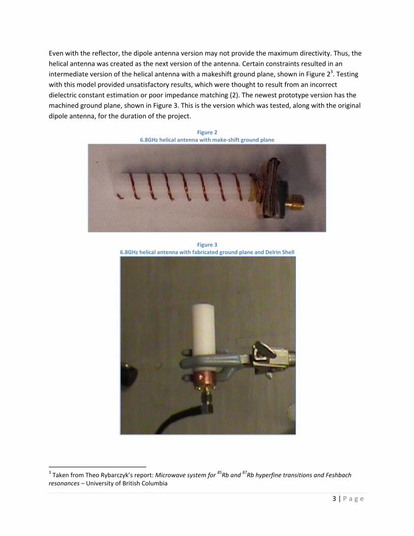
Even with the reflector, the dipole antenna version may not provide the maximum directivity. Thus, the
helical antenna was created as the next version of the antenna. Certain constraints resulted in an
intermediate version of the helical antenna with a makeshift ground plane, shown in Figure 23. Testing
with this model provided unsatisfactory results, which were thought to result from an incorrect
dielectric constant estimation or poor impedance matching (2). The newest prototype version has the
machined ground plane, shown in Figure 3. This is the version which was tested, along with the original
dipole antenna, for the duration of the project.
Figure 2
6.8GHz helical antenna with make-shift ground plane
Figure 3
6.8GHz helical antenna with fabricated ground plane and Delrin Shell
3 Taken from Theo Rybarczyk’s report: Microwave system for
85Rb and
87Rb hyperfine transitions and Feshbach
resonances – University of British Columbia

4 | P a g e
The helical antenna’s dimensions are easily altered through the use of a dielectric core. An initial
problem with the helical antenna was the antenna length, as a small antenna is required for the
experiment. As an example, the 3.0GHz model had a calculated length of 22.2cm for a helical loop in a
vacuum. The required length of the helix is proportional to the wavelength; therefore it may be reduced
by having a core and shell material with a large dielectric constant.
1.3 Technical Requirements
As stated above, the antenna must exhibit high directivity and be as small and robust as possible. There
is no stated minimum length or size for the antenna. The objective of the project is to balance size and
intensity to create an antenna which will transfer maximum radiation to the Rubidium Dipole Trap as
efficiently as possible. The size of the antenna can be quantified by viewing the source field from the
dipole trap. The solid angle created by the antenna takes into account both the size of the antenna and
the distance from the dipole trap. Therefore, the solid angle should be taken into account when
quantifying the final version.
One specification which arises from the project outline is the aspect of impedance matching. To transfer
the microwave signal efficiently, the microwave antenna should have 50Ω input impedance. This is
especially an issue in the case of the helical antenna, where the input impedance is directly proportional
to the helix circumference. This is discussed more in the theory segment of the discussion section.
Another technical requirement, which is mostly for ease of integration into the existing system, is the
use of SMA connections between the antenna and RbSS. SMA connectors also have a 50Ω input
impedance and perform adequately in the 3.0GHz and 6.8GHz range. Both the existing dipole and
helical antennas were designed with SMA connections, as is the final design.
1.4 Industrial Competitors – Alternative Strategies
Fractal Antenna Systems Inc. design and manufacture antennas for commercial, military, and
government applications. Fractal Antenna Systems designs antennas using fractal geometry, enabling
them to manufacture antennas which are 50 to 75 percent smaller than traditional antennas (3).
Furthermore, using fractal geometry allows for a higher number of resonant frequencies than traditional
antenna designs. Furthermore, Fractal Antenna Systems has a comprehensive design process in which
its team of engineers conducts works with the customer from the project definition to the product
production phase. This company was not pursued as a possible source of microwave antenna fabrication
due to time and cost constraints.
Other options for the final design included selecting from any of the various antenna types. The project
goal was to test and characterize the existing prototypes and use the data to generate an optimal final
design. Therefore, it did not appear to be in the best interest of the team to develop a third prototype of
an entirely different design such as horn, parabolic, or spiral, which would then have to be tested,
characterized, compared, and fine-tuned before an optimal version is produced.

5 | P a g e
2. Discussion
The following sections outline the project objectives, technical background and theory, methods and
experimental set-up, and final designs.
2.1 Project Objectives
The project objectives for this project include characterizing the current antenna designs, researching
alternate antenna types and materials, establishing a final design, and determining characteristics of the
final antenna. These are described in more detail in the following sub sections.
Objective 1: Characterization of Existing Antennas
There are currently two antennas available for characterisation. The first is a dipole antenna which has
already undergone testing, although the tests will be repeated by the team for project consistency. The
team will measure the antennas impedance, reflectance, and emission pattern. The emission pattern for
antennas can be characterized in terms of two quantities: the gain and the intensity distribution. The
second prototype is a helical antenna with a Delrin core. Similarly to the dipole antenna, the team will
measure the antenna impedance, reflectance, and emission pattern. In addition to these parameters,
the exact dielectric constant of Delrin at both 3.0GHz and 6.8GHz must also be determined.
Objective 2: Research Alternate Designs and Materials
There are many types of antennas, including dipole, helical, biconical, sleeve, and spiral, as well as many
ways of fabricating each (see section on Fractal Antenna Systems, above). The various antenna type and
fabrication options will be researched in order to determine which antenna is optimal for the specific
experiment. The deliverable for this objective will be to establish an ideal shape, material, and
fabrication process for the antenna in order to begin working on a final design.
Objective 3: Establish Final Design
A final design for an optimal antenna which is both robust and reproducible is required for Objective 3.
This includes placing all orders for parts and materials, as well as all submitting machine shop work
orders. Drawings must be completed to provide the machine shop with an outline of the antenna shape
and to help with antenna fabrication.
Objective 4: Characterizing the Final Antenna
The final version of the antenna must be characterized in the same manner as the prototypes. The team
will measure the antenna impedance, reflectance, and emission pattern. Any unforeseen changes to the
antenna design should be accounted for in a new drawing set for the final design package.

6 | P a g e
2.2 Technical Background and Theory
This section outlines the additional theory required to describe the project, which has been developed in
the time proceeding the initial project proposal.
2.2.1 Helical Antennas: Theory of Antenna Arrays and Parasitic Antennas
As mentioned in Objective 2 of the project objectives section above, the team is to research
alternate designs to improve antenna gain and directionality. It is the opinion of the team that the
helical antenna gives the greatest directionality and intensity when operated in its axial mode. In this
context, axial mode implies that the radiation pattern is parallel to the helical axis, having the maximum
of the radiated power in the direction of cylinder axis. A literature search has shown that there are two
common methods to further increase the gain and directionality of the helical antenna: creating
symmetric antenna arrays and modifying winding design to include parasitic antennas.
Arrays of Monofilar Axial-Mode Helical Antennas
The novelty behind the array of monofilar axial-mode helical antennas is that it maintains the single
antenna emission pattern characteristics (highly directional radiation emission pattern) while increasing
the gain. A diagram showing how the array is arranged is shown below in Figure 4.
Figure 4
The 2 by 2 Antenna Array front view (left) and side view (right). A1, A2, A3 and A4 represent individual helical antenna
elements and d is the displacement between them. The antennas are mounted on a reflecting back-plate.
Let the desired output wavelength of the system to be λ. The distance between adjacent antennas in the
2 by 2 system have been experimentally been chosen to be 1.5 λ (4), both horizontally and vertically (d =
1.5 λ). This configuration produces the most symmetry of the main lobe in both E and H polarizations,
yielding maximum directional gain.
After measuring the output radiation pattern of a single helical antenna (which has been done during
the course of this project), we obtain an emission pattern R(r, θ, φ). To demonstrate the effect of the
array, the antenna array factor for N antenna elements (AF)N must be defined.

7 | P a g e
Given R(r, θ, φ), the emission pattern of the array can be approximated (to within 20%) by
���, �� � ��, �� ����
Where, for a uniformly spaced N element array,
���� � ������������������������� �!"�#����$
Here, k is the wave number and d is the distance between array elements.
Therefore, for the N=4 array designed for this project,
���% � ���&'����������(%������� �!"�#����$
And
���, �� � ��, �� sin,2./�012�31�54sin�12kd�cosθ31��$
From this it is apparent the maximum radiation intensity still occurs along the axis θ = 0°.
To further prove that directionality is improved using the array, the directionality of the N=1 element
and the N=4 element array will be compared.
The measure of directionality of a single helix is given by
<�,�=>?@A B 12CD'EF%
Where n is the number of turns in the helix, S is the spacing between two adjacent windings and C is the
circumference of a single turn. The implemented design (G = 6.8 GHz) has n = 8, C = 0.06 m, and
S = 0.006 m giving <�,�=>?@A B 24.1.
The directionality of the 2 by 2 array is given by
<I,JKKJL � MNJOM�
Where Umax is the maximum intensity value of y(θ,φ) and is taken to be 1 and M� B P'���

8 | P a g e
Therefore,
<I,JKKJL B 2Q./R � 4Q S/FT � 4 S1 U V
/T
Or by implementing the Hansen-Woodyard approximation for antenna arrays, the directivity is given by
<I,JKKJL � MNJOM� � 10.554 Y
2Q./R Z � 1805 Y4Q S/FTZ
Given N = 4, d = 1.5F: <I,JKKJL B 43300
So it has been shown that <I,JKKJL >> <I,�=>?@A and the use of the array is justified and beneficial for
large directionality increases.
To address gain increases, it must be indicated that each element of the array has an associated - and
approximately identical – impedance Z, and by the law of adding parallel impedances the impedance of
the N=4 array is given by
\JKKJL � \||Z||Z||Z � Z4
So the array impedance of the array is one quarter that of a single antenna, which given a constant
source power input, will yield a higher output gain.
In conclusion, the helix-antenna array will generate an output which is more directional and has a higher
gain than that of a single antenna element. If the array does not break the solid angle constraints
needed for the project sponsor’s optical arrangement, this option will be a significant improvement on
the original antenna design.
Helix-Helix Parasitic Elements
A parasitic antenna (or passive radiator) is a radio antenna which is not connected to its source by a
wire. This added element absorbs radiation from surrounding antennas and re-radiates it, which leads to
higher directionality and thus higher intensity in the axial direction. During spatial emission pattern
characterization experiments, it was noticed that there was a significant amount of radiation produced
non-axially. This added element will redirect a portion of this radiation and force it to propagate axially.
Figure 5 below shows how the parasitic element will be placed with respect to the original helical
antenna.
Figure 5
Helix-Helix parasitic antenna element. The Driven Antenna (red) is powered directly from the RbSS, and the Parasitic
Antenna (blue) is not powered, but rather directs the non-axial radiation from the Driven Antenna, increasing directionality.

9 | P a g e
John D. Kraus, the inventor of the helical antenna, reports the following in his textbook Antennas 2nd
Ed.
(1988) on the gain increase and improved directionality of this helix-helix parasitic antenna modification
(5):
“If a parasitic helix is wound between the turns of a driven monofilar axial-mode helical antenna without
touching it (diameters the same), Nakano et al. report that the combination gives an increased gain of
about 1 dB without an increase in the axial length of the antenna. The increased gain occurs for helices
of any number of turns between 8 and 20. The parasitic helix may be regarded as a director for the
driven helix.”
With these experimentally established advantages of the parasitic helix addition, we have confirmed its
use in our final design.
The theory presented by the reference materials for these methods treats helical antenna arrays and
parasitic helical antennas separately, i.e., the concept of an array of parasitic helical antennas is not
mentioned. Without experimentally quantitatively verifying the performance increases found by
combining both methods, it can be loosely argued that having a large reflecting back plate from the
antenna array will direct a large portion of the non-axial radiation back toward the parasitic antennas,
which trap the waves, re-directing it axially. Likewise for adjacent antennas: each individual helix will
emit some radiation radially instead of axially, and there will be three parasitic antennas available to
redirect this radiation towards the target.

10 | P a g e
2.3 Methods and Experimental Equipment
This section focuses on the equipment used to characterize the two prototype antennas. The testing
equipment consisted of unique apparatus such as the Rubidium State Selector (RbSS) and antennas, as
well as commercial measurement equipment. A DC voltage supply was used to supply power to the RbSS
phase locked loop (PLL) and power amplification loop. The reference signal for the PLL was supplied by a
function generator, which outputted an 85MHz signal for the 6.8GHz antenna testing. The antenna
signal transmitted to the antenna pick-up. A pick-up was assembled at the beginning of the project,
however a second pick-up was later used which provided increased signal stability during testing. Figure
6 display the testing set-up used during the project, with standard equipment parameters. The following
sections describe the equipment used in the experimental set-up.
Figure 6
Testing set-up for frequency variation and spatial distribution characterization of prototype antennas
11 | P a g e
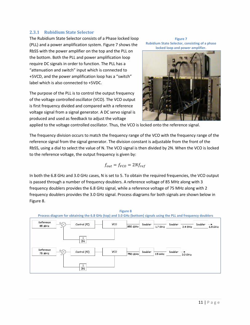
2.3.1 Rubidium State Selector
The Rubidium State Selector consists of a Phase locked loop
(PLL) and a power amplification system. Figure 7 shows the
RbSS with the power amplifier on the top and the PLL on
the bottom. Both the PLL and power amplification loop
require DC signals in order to function. The PLL has a
“attenuation and switch” input which is connected to
+5VCD, and the power amplification loop has a “switch”
label which is also connected to +5VDC.
The purpose of the PLL is to control the output frequency
of the voltage controlled oscillator (VCO). The VCO output
is first frequency divided and compared with a reference
voltage signal from a signal generator. A DC servo signal is
produced and used as feedback to adjust the voltage
applied to the voltage controlled oscillator. Thus, the VCO is locked onto the reference signal.
The frequency division occurs to match the frequency range of the VCO with the frequency range of the
reference signal from the signal generator. The division constant is adjustable from the front of the
RbSS, using a dial to select the value of N. The VCO signal is then divided by 2N. When the VCO is locked
to the reference voltage, the output frequency is given by:
G�_` � Gabc � 2QGKAd
In both the 6.8 GHz and 3.0 GHz cases, N is set to 5. To obtain the required frequencies, the VCO output
is passed through a number of frequency doublers. A reference voltage of 85 MHz along with 3
frequency doublers provides the 6.8 GHz signal, while a reference voltage of 75 MHz along with 2
frequency doublers provides the 3.0 GHz signal. Process diagrams for both signals are shown below in
Figure 8.
Figure 7
Rubidium State Selector, consisting of a phase
locked loop and power amplifier.
Figure 8
Process diagram for obtaining the 6.8 GHz (top) and 3.0 GHz (bottom) signals using the PLL and frequency doublers

12 | P a g e
The purpose of the power amplifier is to amplify the signal to around 1W. The output power from the
RbSS is controlled with a set-point voltage, supplied by a DC voltage source, which should be between
4V and 10V. The output of the PLL is connected via SMA to the input of the power amplifier, and the
output is sent to the antenna. The power amplifier also has a control loop to ensure a constant power
output. More information on both the PLL and power amplification loop is found in Theo Rybarczyk’s
report: Microwave system for 85
Rb and 87
Rb hyperfine transitions and Feshbach resonances – University
of British Columbia (2).
One observed issue with the RbSS output is that the output spectrum has additional peaks. Figure 9
below shows the trace data from the spectrum analyzer for an RbSS intended output of 6.8GHz. There is
an additional peak, 85MHz below the expected peak, at 5.95GHz. This peak is not expected, and is not
seen under the characterization testing span of 2.0MHz.
Figure 9
RbSS trace data from the spectrum analyzer for expected frequency of 6.8GHz, with additional peak at 5.95GHz.
The reference signal required to produce a 6.8GHz signal is 85MHz, which is then multiplied by 10 and
doubled 3 times as discussed above. Therefore, the extra peak may be due to defects in the frequency
doubler and band-pass filter stages. This result is very reproducible, and because it was not recorded in
the spectrum analyzer trace span of 2MHz, it is ignored in the remainder of the report.
-65
-60
-55
-50
-45
-40
-35
-30
5.4E+09 5.9E+09 6.4E+09 6.9E+09 7.4E+09
Inte
nsi
ty (
dB
m)
Frequency (Hz)
Trace Data from RbSS Output
13 | P a g e
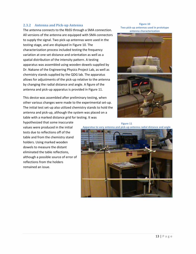
2.3.2 Antenna and Pick-up Antenna
The antenna connects to the RbSS through a SMA connection.
All versions of the antenna are equipped with SMA connectors
to supply the signal. Two pick-up antennas were used in the
testing stage, and are displayed in Figure 10. The
characterization process included testing the frequency
variation at one set distance and orientation as well as a
spatial distribution of the intensity pattern. A testing
apparatus was assembled using wooden dowels supplied by
Dr. Nakane of the Engineering Physics Project Lab, as well as
chemistry stands supplied by the QDG lab. The apparatus
allows for adjustments of the pick-up relative to the antenna
by changing the radial distance and angle. A figure of the
antenna and pick-up apparatus is provided in Figure 11.
This device was assembled after preliminary testing, when
other various changes were made to the experimental set-up.
The initial test set-up also utilized chemistry stands to hold the
antenna and pick-up, although the system was placed on a
table with a marked distance grid for testing. It was
hypothesized that some inaccurate
values were produced in the initial
tests due to reflections off of the
table and from the chemistry stand
holders. Using marked wooden
dowels to measure the distant
eliminated the table reflections,
although a possible source of error of
reflections from the holders
remained an issue.
Figure 10
Two pick-up antennas used in prototype
antenna characterization
Figure 11
Apparatus to vary antenna and pick-up antenna radial distance and angle
14 | P a g e
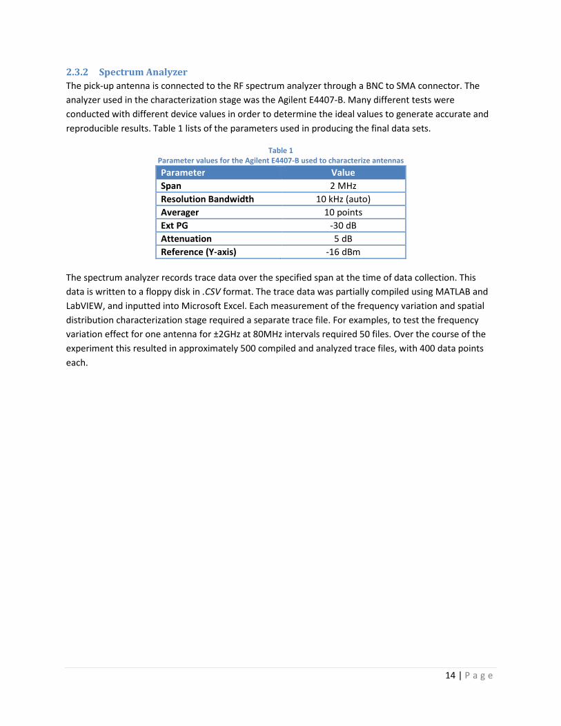
2.3.2 Spectrum Analyzer
The pick-up antenna is connected to the RF spectrum analyzer through a BNC to SMA connector. The
analyzer used in the characterization stage was the Agilent E4407-B. Many different tests were
conducted with different device values in order to determine the ideal values to generate accurate and
reproducible results. Table 1 lists of the parameters used in producing the final data sets.
Table 1
Parameter values for the Agilent E4407-B used to characterize antennas
Parameter Value
Span 2 MHz
Resolution Bandwidth 10 kHz (auto)
Averager 10 points
Ext PG -30 dB
Attenuation 5 dB
Reference (Y-axis) -16 dBm
The spectrum analyzer records trace data over the specified span at the time of data collection. This
data is written to a floppy disk in .CSV format. The trace data was partially compiled using MATLAB and
LabVIEW, and inputted into Microsoft Excel. Each measurement of the frequency variation and spatial
distribution characterization stage required a separate trace file. For examples, to test the frequency
variation effect for one antenna for ±2GHz at 80MHz intervals required 50 files. Over the course of the
experiment this resulted in approximately 500 compiled and analyzed trace files, with 400 data points
each.

15 | P a g e
2.4 Results
To characterize the original antenna prototypes, the team determined the frequency dependencies and
the spatially dependent emission patterns of the 6.8 GHz helical and 6.8 GHz dipole antennas. The
results of these tests are used to modify the designs to maximize gain and directionality at the desired
frequency (6.8GHz or 3.0 GHz). The experiments were performed in the Quantum Degenerate Gas
laboratory at the University of British Columbia with the Rubidium State Selector as the source and
Agilent Model E4407B radio frequency spectrum analyzer as the measuring receiver.
2.4.1 Frequency Dependency
The frequency study was used to determine the frequency response of each antenna. To maximize gain,
the largest intensity amplitudes should lie on the target frequency (6.8 GHz or 3.0 GHz). The frequency
dependency of an antenna is dependent on its physical parameters such as winding circumference and
core material dielectric constant, so this experiment provides insight into how to alter the design to
improve gain.
The frequency experiment was performed on the 6.8 GHz helical and dipole antennas by taking
spectrum intensity readings for values between 4.8 GHz and 7.8 GHz in increments of 80 MHz. Both sets
of data have been normalized with a baseline dataset taken directly from the Rubidium State Selector.
Figure 12 and Figure 13 are a summary of experimental results, as intensity and gain plots respectively.
Figure 12
Intensity vs. Frequency for both the 6.8 GHz helical antenna and the 6.8 GHz dipole antenna
-20
-18
-16
-14
-12
-10
-8
-6
-4
-2
0
2
4
6
8
10
4.6 4.8 5 5.2 5.4 5.6 5.8 6 6.2 6.4 6.6 6.8 7 7.2 7.4 7.6 7.8
Inte
nsi
ty (
dB
m)
Frequency (GHz)
Intensity vs. Frequency
Helix
Dipole

16 | P a g e
Figure 13
Antenna output gain vs frequency. This further exemplifies the shifted maximum peak of the helical antenna gain.
2.4.2 Spatial Emission Pattern
The purpose of the spatial emission pattern
experiment is to analyze the antenna directivity
and choose a suitable antenna type for the final
prototype design. The horizontal plane (i.e., the
plane with no vertical antenna emission
inclination with respect to the receiving antenna)
was decided to be suitable for characterizing
spatial intensity dependence. This is a valid
generalization because the target for the
Rubidium spin manipulation experiment will also lie in this plane (axially, most likely).
0
0.25
0.5
0.75
1
1.25
1.5
1.75
2
2.25
2.5
4.5 4.7 4.9 5.1 5.3 5.5 5.7 5.9 6.1 6.3 6.5 6.7 6.9 7.1 7.3 7.5 7.7
Ga
in
Frequency (GHz)
Gain vs. Frequency
Helix
Dipole
Figure 14
Top view of antenna showing sweeping method of measuring
planar emission pattern

17 | P a g e
To measure the emission pattern, set displacements were measured at the desired center frequency
(6.8 GHz) and at various angles as shown below, to sweep out a plane of data points. Varying angles
θ:[0°,180°] in increments of 30°, and varying distances d:[10cm, 100 cm], an array of raw intensity data
points were collected. For each antenna the raw intensity data was normalized to the maximum of its
set and plotted as a two dimensional contour plots. The results of this experiment are shown below in
Figure 15.
Figure 15
Horizontal plane emission patterns. The normalized intensity of the 6.8 GHz helical antenna (left) and the 6.8 GHz dipole
antenna (right) have been plotted to compare directivity.

18 | P a g e
2.5 Discussion of Results
The final antenna prototype designs were decided upon partially by the results of the frequency
dependency and spatial emission pattern experiments and also from theoretical models which are
described in the theory section of this report. The following sections summarize the important findings
of each experiment and what the conclusions have lead to with regard to design alterations.
2.5.1 Spatial Emission Pattern
The spatial emission pattern is used to compare the antenna types. As seen in Figure 15, the dipole
antenna bleeds more radiation non-axially close to the antenna output compared with the helical
antenna. This characteristic leads to an undesirable lower intensity in the axial direction. When
analyzing just the axial emission pattern (the intensity along the vertical line directly above the antenna
output), the dipole exhibits large regions of low intensity compared to the helix. These factors have
directed the team to choose the helical antenna type for the final prototype.
2.5.2 Frequency Dependency
The results of the frequency dependency experiment strengthen the choice for a helical antenna for the
final prototype design. In Figure 13 it is apparent that the gain of the helical antenna is generally higher
than the dipole. This is likely due to the radial bleeding described in the section above. The dipole
antenna frequency response will not be discussed as the helical antenna proves to be better suited for
this application.
Looking now at the helix antenna response, there is a significant rise in gain around 6 GHz, implying that
the antenna tested here is not best suited to operate at 6.8 GHz. This frequency response is dependent
on the circumference of the helix as well as the dielectric of the core material, and can be altered to
perform better at 6.8 GHz in the following way:
The antenna which has been tested operates best at approximately λo = 0.05 m and we would like the
next prototype to operate at λ = 0.0271 m. In order to achieve axial radiation from a helical antenna
must have C and pitch angle α such that
λλ3
4
4
3<< C And
oo1512 << α .
The tested antenna has helix circumference Co = 28mm = 1.2 λ, which is within the required bounds but
may be producing the offset. We have therefore chosen to use the midpoint of both the above bounds
in an attempt to shift the maximum intensity to λ = 0.0271 m, i.e. C = 1.042 λ and α =13.5o.
To calculate a new circumference we need to know the dielectric constant of delrin rε , the core
material.
05.04.30271.0
050.022
±=
=
=
λ
λε
o
r
Working backwards now using the same dielectric material, set λ = ro ελ / , == fco /λ 3.0x10⁸
/
6.8x10⁹, we get λ =0.0239 m and C = (1.042)(0.0239) = 0.025 ± 0.005 m.

19 | P a g e
We would like to minimize the length of the antenna and fewer turns will yield a shorter helix. Since N =
8 is the minimum turns required to utilize the parasitic effect, this will be the number of turns for the
final design. The length of a single turn is calculated from the pitch angle and circumference:
mCl 0005.00060.0)5.13(tan)025.0()(tan011
±===−−
α
The total antenna length is therefore )0060.0)(8(== NlL = 0.048 ± 0.0005 m.
Now knowing the dielectric constant, the same calculations can be performed and a summary of these
results can be found in Table 2.
The spatial emission pattern experiment has led to the choice of the helical type antenna for the final
design due to the increase in directionality and axial radiation intensity when compared to the dipole
antenna. The frequency characterization experiment shows that the first prototype helix is not
optimized for 6.8 GHz, but gives us a way to calculate the dielectric constant of Delrin and determine the
optimal physical parameters of the antenna to output 6.8 GHz while still having parasitic ability.

20 | P a g e
2.6 Final Design
As shown in the results section above, the helical antenna exhibited high directivity than the dipole
antenna. This was the basis for selecting the helical antenna for the final design. Furthermore, the
impedance matching to 50Ω is accomplished though the use of an antenna array system, which in
conjunction with the parasitic helix wire will also further increase the directivity. This section contains
calculations for the single antenna dimensions as well as descriptions of the parasitic and array antenna
structures. Dimensioned drawings are available in Appendix A.
Shown above, the dielectric constant of Delrin, initially thought to be 3.5, is calculated as 3.393. This
material was chosen as the final design material due to numerous factors including cost, ease of
machining, and because the current Delrin model is already characterized. Other materials are discussed
in the Alternative Designs section of the report.
2.6.1 Design Calculations
This section provides an outline of the calculations used in the final design of a Delrin core helical
antenna. The wavelength in a vacuum, λo, is calculated as:
FI�6.8fgh� � 0�G � 299792458 k 2⁄6.8 m 10n2�� � 0.04409 k
FI�3.0fgh� � 0�G � 299792458 k 2⁄3.0 m 10n2�� � 0.1 k
The required circumference of the helix is designed such that it will be in the middle of the
circumference range for an axial mode of radiation. Averaging the bounds on the circumference (see
Technical Background and Theory section) suggests that the circumference should be 1.042 times the
wavelength. The wavelength in the dielectric is scaled by its dielectric constant; therefore, the
circumference of both antennas can be calculated from λo and the experimentally determined dielectric
constant.
Dp�6.8fgh� � 1.042�F� � 1.042 YF��6.8fgh�qK Z � 0.02494 k
Dp�3.0fgh� � 1.042�F� � 1.042 YF��3.0fgh�qK Z � 0.05653 k
The circumference values in addition to the selection of the helical pitch angle and number of turns
generate values for the helix diameter and length. The pitch angle was selected at 13.50 as the average
of the upper and lower bounds for an axial mode of radiation. The number of turns was selected at the
minimum number of turns in which the parasitic antenna will function to increase the antenna
directivity. The helix parameters for the 6.8GHz and 3.0GHz models are shown in Table 2.
21 | P a g e
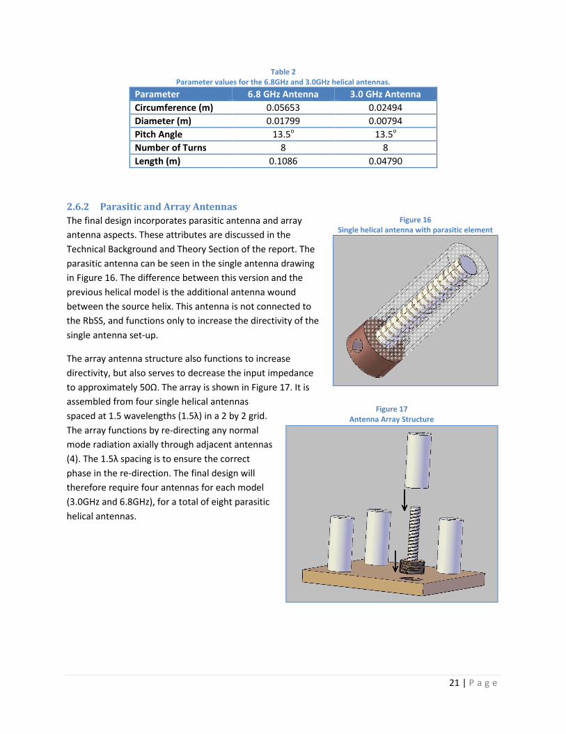
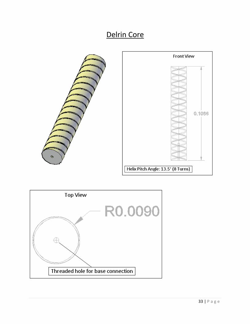
Table 2
Parameter values for the 6.8GHz and 3.0GHz helical antennas.
Parameter 6.8 GHz Antenna 3.0 GHz Antenna
Circumference (m) 0.05653 0.02494
Diameter (m) 0.01799 0.00794
Pitch Angle 13.5o 13.5
o
Number of Turns 8 8
Length (m) 0.1086 0.04790
2.6.2 Parasitic and Array Antennas
The final design incorporates parasitic antenna and array
antenna aspects. These attributes are discussed in the
Technical Background and Theory Section of the report. The
parasitic antenna can be seen in the single antenna drawing
in Figure 16. The difference between this version and the
previous helical model is the additional antenna wound
between the source helix. This antenna is not connected to
the RbSS, and functions only to increase the directivity of the
single antenna set-up.
The array antenna structure also functions to increase
directivity, but also serves to decrease the input impedance
to approximately 50Ω. The array is shown in Figure 17. It is
assembled from four single helical antennas
spaced at 1.5 wavelengths (1.5λ) in a 2 by 2 grid.
The array functions by re-directing any normal
mode radiation axially through adjacent antennas
(4). The 1.5λ spacing is to ensure the correct
phase in the re-direction. The final design will
therefore require four antennas for each model
(3.0GHz and 6.8GHz), for a total of eight parasitic
helical antennas.
Figure 16
Single helical antenna with parasitic element
Figure 17
Antenna Array Structure

22 | P a g e
2.7 Sources of Error
Wave Reflections
In experiments measuring antenna radiation characteristics, an ideal laboratory would be large enough
to neglect any reflecting waves which may influence intensity measurements. This is not always
practical, however, and was not the case during these experiments. The measurements were taken in
close proximity to large metal, wood and plastic structures, and how these objects manipulate
measurements is still generally unknown. For our purpose (which is to determine emission
characteristics of antennas relative to one another), ensuring the placement of an antenna within the
laboratory was constant for each test allows us to approximately neglect the effects of reflection.
Spectrum Analyzer Resolution Bandwidth and Averaging
In the initial stages of the project, poor results were obtained for both frequency and spatial
experiments. The problem was not with the experimental apparatus used, but with the resolution
bandwidth (RBW) and averager of the spectrum analyzer. Since the intensity measurements fluctuate
significantly from sample to sample the averager must be implemented to yield reliable results. Also, to
obtain sensible results, the RBW of the spectrum analyzer must be selected appropriately to guarantee
appropriate measurement sensitivity. The entire desired spectrum (4.8 GHz to 7.86 GHz) was naively
chosen at first as the RBW, which sent the measured intensity peak levels nearly into the background
noise. Needless to say this data was unusable and had to be retaken, greatly postponing objective
deadlines.
Pick-up Antenna Selection
For the initial experiments, the receiver antenna we used produced signals which were not repeatable
or reliable. Later experiments were done with a smaller receiver and repeatable and stable
measurements were taken. This stability allowed us to gather the qualitative data needed to chose the
correct antenna. For quantitative results it would be necessary to characterize the receiver antenna and
include it as part of the overall system transfer function.

23 | P a g e
3. Conclusions
The characterization of the helical and dipole antenna at 6.8GHz, presented in the results section,
provide a set of baseline data. This baseline data will be compared with data measured for the final
design. Ideally, the final design will exhibit higher directivity than the two previous models.
It is concluded from the baseline data that the optimal antenna form, when choosing between a dipole
antenna and a helical antenna, is the helical antenna. This antenna exhibits higher directivity, and with
some changes to the design is tuned to the correct center frequency.
Research into alternative designs produced information on parasitic and array antennas, both of which
are incorporated into the final design. The final version of the antenna is based on a helical antenna
which is very similar to the current model; with a slightly smaller diameter and length resulting from the
re-calculated dielectric constant of Delrin (ε = 3.393). Also, a parasitic wire is wound between the turns
of the drive antenna to increase the directivity. Four antennas will be fabricated for the 6.8GHz model
and the 3.0GHz model. These will be installed on a ground plate in a 2 by 2 array. The function of the
array is to further increase the directivity and tune the input impedance to 50Ω. Plans have been
submitted to the electrical machine shop for antenna fabrication.
Objective 4, characterization of the final design, is incomplete due to time constraints. Numerous
sources contributed to this including RbSS troubleshooting and incorrect usage of the spectrum analyzer
resolution bandwidth which resulted in the need to reacquire most of the data.

24 | P a g e
4. Recommendations
1. Characterization of new antennas: The procedure used to characterize the emission pattern
and frequency dependency of each antenna should be done in a completely reproducible way.
In general, the laboratory space used to perform these experiments is filled with objects which
may cause reflections that alter measurements. It is important that the researcher be careful to
arrange the antennas in the same fashion each time an experiment is performed to reduce the
relative error incurred by the environment.
2. Construction of new antennas: Since the new antennas are meant to be placed in an array, the
theory is based on the premise that they are identical (same input impedance and helical
parameters). It is therefore necessary to construct each element in a similar fashion to optimize
homogeneity.
3. Selecting appropriate spectrum analyzer settings: We had lost a lot of time collecting unusable
data with the spectrum analyzer because the resolution bandwidth used was too large, creating
intensity readings which were close to background noise level. Staying aware of which RBW is
being used will lead to higher measurement sensitivity and reduction of errors. Also, since the
signal encounters a large amount of noise traveling from the RbSS to the helical antenna, from
the helical antenna to the receiver antenna, and finally from the receiver antenna to the
spectrum analyzer, it is important to average over a reasonable time span (20 data points) to
minimize outside-system influences on measurements.
4. Characterization of receiver antenna: Since our study was focused on obtaining information
about the helical and dipole antennas relative to each other qualitatively, it was not imperative
that the full system transfer function was known since the system is assumed to be linear time-
invariant. When characterizing the final designs, however, the quantitative response of the
antennas will be desired, and the receiver antenna will need to be characterized. This can be
done by placing a fully characterized antenna on the output line of the RbSS and obtaining the
signal through the receiver antenna into the spectrum analyzer. Then the system can be
reversed, i.e. place the receiver antenna on the output line of the RbSS and the characterized
antenna into the spectrum analyzer. The comparison of these two responses will allow the
transfer function of the receiver antenna to be calculated.

25 | P a g e
Bibliography
1. Robinson, Alan. Measuring the Molecular Structures of Ultracold Lithium-Rubidium Dimers by
Feshbach Resonance. Vancouver : University of British Columbia, 2009.
2. Rybarczyk, Theo. Microwave system for 85-RB and 87-RB hyperfine transitions and Feshbach
resonances. Vancouver : University of British Columbia, 2009.
3. Our Technologies: Fractal Antenna Systems. [Online] Fractal Antenna Systems Inc. [Cited: September
25, 2009.] http://www.fractenna.com/index.html.
4. Verification of Four Elements Helical Antennas Array Design Procedure. Zemanovic, Jan, Peter, Hajach
and Podhoransky, Peter. 2008.
5. Kraus, John D. Antennas. 2nd Edition. New York : McGraw-Hill, 1988. 0-07-463219-1.
6. Applications of the Feshbach-resonance management to a tightly confined Bose-Einstein Condensate.
Filetralla, Giovanni, Malomed, Boris A and Salasnich, Luca. 4, April 2, 2009, Physical Review A, Vol. 79.

26 | P a g e
Appendix A – Dimensioned Drawings

27 | P a g e
6.8 GHz Prototype

28 | P a g e
Delrin Shell

29 | P a g e
Delrin Core
Helix Pitch Angle: 13.5° (8 turns)

30 | P a g e
Copper Base

31 | P a g e
3.0 GHz Prototype

32 | P a g e
Delrin Shell
33 | P a g e
Delrin Core

34 | P a g e
Copper Base

35 | P a g e
Appendix B – MATLAB Script for Trace Data Compilation

36 | P a g e
Helix.m
%%%%%%%%%%%%%%%%%%%%%%%%%%%%
% This program imports Spatial Emission Pattern data
% and transcribes peak values to a 3D Grid. This
% particular file is defined FOR HELICAL ANTENNA
% assuming output symmetry
% Structure of Data Files:
% Define the following alpha-to-numeric constants:
% A = 0
% B = 1
% C = 2
% D = 3
% E = 4
% F = 5
% G = 6
% H = 7
% I = 8
% J = 9
% Name Format: _ _ _ _.csv
% (1)(2)(3)(4)
% Positions 1,2, and 3 specify the distance the receiving antenna
% is placed from the emitting antenna, measured in centimeters
% For example: BJD_.dat
% would indicate that the receieving
% antenna was placed 193 cm from emitting
% antenna.
% Position 4 incicates the angle the normal of the receiving
% antenna makes with the negative of the normal of the emitting
% antenna.
% This is coded alphabetically as well:
% S = 0
% T = 45
% U = 90
% V = 135
% W = 180
% X = 225
% Y = 270
% Z = 315
% For example: DABX.csv
% would indicate the receiving antenna
% was placed 301 cm away from the
% emitting antenna with 225 degrees
% between the normal of the receiving
% antenna and the negative of the normal
% of the transmitting antenna.
%%%%%%%%%%%%%%%%%%%%%%%%%%%%%%%%%%%%%%%%%%%%%%%%%%%%%%%%%%%
% Define Character Space for Spatial and Angular File-Specific Coordinates
SPC = ['A','B','C','D','E','F','G','H','I','J', '0'];
NSPC = ['0','1','2','3','4','5','6','7','8','9'];
n = length(SPC);
ANG = ['S','T','U','V','W','X','Y','Z', '0'];
NANG = ['000','045','090','135','180','225','270','315', '000'];
m = length(ANG);
counter = 0;
% Create all possible
% maxima(1,1) = 'frequency';
% maxima(1,2) = 'intensity';
% maxima(1,3) = 'distance';
% maxima(1,4) = 'angle';
for i = 1:m
for j = 1:2
for k = 1:n

37 | P a g e
for l = 1:n
temp = strcat(SPC(j), SPC(k), SPC(l), ANG(i),'.csv');
if exist(temp)==0
else
counter=counter+1;
M1 = csvread(temp, 15);
data = M1(:,1:2);
[C,I] = max(data(:,2));
maxima(counter,1) = max(data(:,2));
%Makes sure max is at 6.8 GHZ
%maxima(counter,1) = data(I,1);
tdist(counter,1) = {strcat(NSPC(j),NSPC(k),NSPC(l))};
tang(counter,1) = {strcat(NANG(3*i-2),NANG(3*i-1),NANG(3*i))};
clear M1 data;
end
end
end
end
end
% Now that all the data has been imported from csv files into matlab:
% Organize the files in terms of angles, and then in terms of distance
for i = 1:counter
if strcmp(tang(i),'045')
for j = 1:10
tt = tdist{i*j};
max45(1,j) = str2num(tt);
max45(2,j) = maxima(i*j);
end
i = i + 10;
elseif strcmp(tang(i),'090')
for j = 1:10
tt = tdist{i*j};
max90(1,j) = str2num(tt);
max90(2,j) = maxima(i*j);
end
i = i + 10;
elseif strcmp(tang(i),'135')
for j = 1:10
tt = tdist{i*j};
max135(1,j) = str2num(tt);
max135(2,j) = maxima(i*j);
end
i = i + 10;
elseif strcmp(tang(i),'180')
for j = 1:10
tt = tdist{i*j};
max180(1,j) = str2num(tt);
max180(2,j) = maxima(i*j);
end
i = i + 10;
elseif strcmp(tang(i),'225')
for j = 1:10
tt = tdist{i*j};
max225(1,j) = str2num(tt);
max225(2,j) = maxima(i*j);
end
i = i + 10;
elseif strcmp(tang(i),'270')
for j = 1:10
tt = tdist{i*j};

38 | P a g e
max270(1,j) = str2num(tt);
max270(2,j) = maxima(i*j);
end
i = i + 10;
elseif strcmp(tang(i),'315')
for j = 1:10
tt = tdist{i*j};
max315(1,j) = str2num(tt);
max315(2,j) = maxima(i*j);
end
i = i + 10;
elseif strcmp(tang(i),'360')
for j = 1:10
tt = tdist{i*j};
max360(1,j) = str2num(tt);
max360(2,j) = maxima(i*j);
end
i = i + 10;
end
end
CONTOURPLOT.m
% Creates the contour plots used to analyze spatial emission patterns of 6.8GHz dipole and
helical %antennas
% Average the results of the angle tests
nHelix = (AngleHelix20(:,3)+AngleHelix30(:,3))/2;
nDipole = (AngleDipole20(:,3)+AngleDipole30(:,3))/2;
% Define Angle and Displacement values
T = [ 180 150 120 90 60 30 0 ];
D = [ 10 20 30 40 50 60 70 80 90 100 ];
for k = 1:length(T)
for j = 1:length(D)
x(j,k) = D(j)*cosd(T(k));
y(j,k) = D(j)*sind(T(k));
end
end
% Normalize the spatial vectors to the average of the angle tests
for i = 1:length(nHelix)
h(:,i) = (DistanceHelix1(:,3) - nHelix(i));
end
for i = 1:length(nDipole)
d(:,i) = DistanceDipole1(:,3) - nDipole(i);
end
h = flipud(h);
d = flipud(d);
subplot(1,2,1);contourf(x,y,h);
subplot(1,2,2);contourf(x,y,d);
clear i j;