Embed Size (px)
Citation preview

The public reporting burden for this collection of information is estimated to average 1 hour per response, including the time for reviewing instructions,
searching existing data sources, gathering and maintaining the data needed, and completing and reviewing the collection of information. Send comments
regarding this burden estimate or any other aspect of this collection of information, including suggesstions for reducing this burden, to Washington
Headquarters Services, Directorate for Information Operations and Reports, 1215 Jefferson Davis Highway, Suite 1204, Arlington VA, 22202-4302.
Respondents should be aware that notwithstanding any other provision of law, no person shall be subject to any oenalty for failing to comply with a collection of
information if it does not display a currently valid OMB control number.
PLEASE DO NOT RETURN YOUR FORM TO THE ABOVE ADDRESS.
a. REPORT
Final Report: Development of Vector Parabolic Equation
Technique for Propagation in Urban and Tunnel Environments
14. ABSTRACT
16. SECURITY CLASSIFICATION OF:
A vector version of parabolic equation (PE) was used to study the 3D propagation of electromagnetic waves in
enclosed structures such as tunnels. The tunnels walls could be lossy, rough, gently curved, or branched. The PE
was solved numerically by adopting the Alternate Direction Implicit finite difference technique. Extensive
comparisons with experimental results conducted by other researchers were carried out to elaborate on the accuracy
and limitations of the technique.
1. REPORT DATE (DD-MM-YYYY)
4. TITLE AND SUBTITLE
12-09-2010
13. SUPPLEMENTARY NOTES
The views, opinions and/or findings contained in this report are those of the author(s) and should not contrued as an official Department
of the Army position, policy or decision, unless so designated by other documentation.
12. DISTRIBUTION AVAILIBILITY STATEMENT
Approved for Public Release; Distribution Unlimited
UU
9. SPONSORING/MONITORING AGENCY NAME(S) AND
ADDRESS(ES)
6. AUTHORS
7. PERFORMING ORGANIZATION NAMES AND ADDRESSES
U.S. Army Research Office
P.O. Box 12211
Research Triangle Park, NC 27709-2211
15. SUBJECT TERMS
Parabolic Equation, Electromagnetic Wave Propagation, Tunnels, Transform Techniques, Stochastic Techniques
Ramakrishna Janaswamy
University of Massachusetts - Amherst
Office of Grant & Contract Admin.
408 Goodell Building
Amherst, MA 01003 -3285
REPORT DOCUMENTATION PAGE
b. ABSTRACT
UU
c. THIS PAGE
UU
2. REPORT TYPE
Final Report
17. LIMITATION OF
ABSTRACT
UU
15. NUMBER
OF PAGES
5d. PROJECT NUMBER
5e. TASK NUMBER
5f. WORK UNIT NUMBER
5c. PROGRAM ELEMENT NUMBER
5b. GRANT NUMBER
5a. CONTRACT NUMBER
W911NF-04-1-0228
611102
Form Approved OMB NO. 0704-0188
45599-EL.1
11. SPONSOR/MONITOR'S REPORT
NUMBER(S)
10. SPONSOR/MONITOR'S ACRONYM(S)
ARO
8. PERFORMING ORGANIZATION REPORT
NUMBER
19a. NAME OF RESPONSIBLE PERSON
19b. TELEPHONE NUMBER
Ramakrishna Janaswamy
413-545-0937
3. DATES COVERED (From - To)
1-Jun-2004
Standard Form 298 (Rev 8/98)
Prescribed by ANSI Std. Z39.18
- 30-Nov-2008

Final Report: Development of Vector Parabolic Equation Technique for Propagation in Urban and Tunnel
Environments
Report Title
ABSTRACT
A vector version of parabolic equation (PE) was used to study the 3D propagation of electromagnetic waves in enclosed structures such as
tunnels. The tunnels walls could be lossy, rough, gently curved, or branched. The PE was solved numerically by adopting the Alternate
Direction Implicit finite difference technique. Extensive comparisons with experimental results conducted by other researchers were carried
out to elaborate on the accuracy and limitations of the technique.
The angular correlation of received fields in 2D multipath environments was studied through full-wave Monte Carlo simulations. The results
showed that the uncorrelated scattering assumption remains valid for the discrete finite spectra when the scattering objects are distributed
randomly and that the correlation among wave components from different angles increases only when the randomness of the scatterer
distribution is reduced.
Separately, expressions for the transitional probabilities for a four-state random walk (FRW) that is used to solve the PE in free-space and
with material boundaries were derived by using transform techniques. An absorbing boundary condition for use with the FRW was also
derived using transform techniques. Appropriateness of the random walk technique for wave propagation problems was demonstrated.
(a) Papers published in peer-reviewed journals (N/A for none)
R. Martelly and R. Janaswamy, ``Modeling radio transmission loss in curved, branched and rough-walled tunnels with the ADI-PE
method,’’ IEEE Trans. Antennas Propagat., vol. 58(6), pp. 2037-2045, June 2010.
J. Xu and R. Janaswamy, ``Angular correlation properties with random multiple scattering,’’ IEEE Trans. Signal Proccessing, vol. 57(7), pp.
2651-2659, July 2009.
R. Martelly and R. Janaswamy, ``An ADI-PE approach for modeling radio transmission loss in tunnels,’’ IEEE Trans. Antennas Propagat.,
vol. 57(6), pp. 1759-1770, June 2009.
R. Janaswamy, ``Transitional probabilities for the four-state random walk on a lattice in the presence of partially reflecting boundaries,’’ J.
Mathematical Physics, vol. 50(5), Pages: 053301 (11 pp), May 2009.
R. Janaswamy, ``Transparent boundary condition for the parabolic equation modeled by the 4RW,’’ IEEE Antennas Wireless Propagat.
Lett., vol. 8, pp. 23-26, 2009.
R. Janaswamy, ``Transitional probabilities for the 4-state random walk on a lattice,’’ J. Phys. A: Math. Theor., vol. 41, Pages: 155306
(11pp), April 2008.
List of papers submitted or published that acknowledge ARO support during this reporting
period. List the papers, including journal references, in the following categories:
(b) Papers published in non-peer-reviewed journals or in conference proceedings (N/A for none)
6.00Number of Papers published in peer-reviewed journals:
Number of Papers published in non peer-reviewed journals:
R. Janaswamy, ``A four state random walk technique for treating the parabolic equation,'' 2009 Joint IEEE International Symposium/URSI
National Radio Science Meeting, Charleston, SC, 2009.
(c) Presentations
0.00
Number of Presentations: 1.00
Non Peer-Reviewed Conference Proceeding publications (other than abstracts):

Number of Non Peer-Reviewed Conference Proceeding publications (other than abstracts): 0
Peer-Reviewed Conference Proceeding publications (other than abstracts):
R. Martelly and R. Janaswamy, ``Propagation prediction in rough and branched tunnels by the ADI-PE techniqu,'' IEEE International
Conference on Electromagnetics in Advanced Applications, ICEAA '09., Digital Object Identifier: 10.1109/ICEAA.2009.5297359,
Publication Year: 2009 , Page(s): 596 - 599.
R. Martelly and R. Janaswamy, ``Propagation in tunnels using the parabolic equation and the ADI technique,'' IEEE Antennas and
Propagation Society International Symposium, Digital Object Identifier: 10.1109/APS.2007.4395426, Publication Year: 2007 , Page(s): 45 -
48.
R. Janaswamy, ``Solution of BVPs in electrodynamics by stochastic methods,''
IEEE Applied Electromagnetics Conference, Digital Object Identifier: 10.1109/AEMC.2007.4638046, Publication Year: 2007 , Page(s): 1 -
4.
(d) Manuscripts
Number of Peer-Reviewed Conference Proceeding publications (other than abstracts): 3
Number of Manuscripts: 0.00
Patents Submitted
Patents Awarded
Graduate Students
PERCENT_SUPPORTEDNAME
Richard Martelly 0.80
Jie Xu 0.05
0.85FTE Equivalent:
2Total Number:
Names of Post Doctorates
PERCENT_SUPPORTEDNAME
FTE Equivalent:
Total Number:
Names of Faculty Supported
National Academy MemberPERCENT_SUPPORTEDNAME
Ramakrishna Janaswamy 0.08 No
0.08FTE Equivalent:
1Total Number:
Names of Under Graduate students supported

PERCENT_SUPPORTEDNAME
FTE Equivalent:
Total Number:
The number of undergraduates funded by this agreement who graduated during this period with a degree in
science, mathematics, engineering, or technology fields:
The number of undergraduates funded by your agreement who graduated during this period and will continue
to pursue a graduate or Ph.D. degree in science, mathematics, engineering, or technology fields:
Number of graduating undergraduates who achieved a 3.5 GPA to 4.0 (4.0 max scale):
Number of graduating undergraduates funded by a DoD funded Center of Excellence grant for
Education, Research and Engineering:
The number of undergraduates funded by your agreement who graduated during this period and intend to
work for the Department of Defense
The number of undergraduates funded by your agreement who graduated during this period and will receive
scholarships or fellowships for further studies in science, mathematics, engineering or technology fields:
0.00
0.00
0.00
0.00
0.00
0.00
......
......
......
......
......
......
Student MetricsThis section only applies to graduating undergraduates supported by this agreement in this reporting period
The number of undergraduates funded by this agreement who graduated during this period: 0.00......
Names of Personnel receiving masters degrees
NAME
Total Number:
Names of personnel receiving PHDs
NAME
Richard Martelly
Jie Xu
2Total Number:
Names of other research staff
PERCENT_SUPPORTEDNAME
FTE Equivalent:
Total Number:
Sub Contractors (DD882)

Inventions (DD882)

Solution of BVPs in Electrodynamics byStochastic Methods
(Invited Paper)
R. JanaswamyDepartment of Electrical & Computer Engineering
University of Massachusetts, Amherst, MA 01002, USA. Email: [email protected]
Abstract-Field computation by the stochastic differentialequation (SDE) method is demonstrated for electrostaticand electrodynamic propagation problems by consider-ing simple examples. The solution to the inhomogeneousHelmholtz equation is first related to that a Schrndingertype of equation (parabolic in nature) by means of Laplacetransformation. The SDE method is directly applied to thisparabolic equation. Presence of the imaginary term in theparabolic equation warrants analytic continuation into thecomplex space that is addressed in this paper.
I. Introduction
SDE methods are alternative methods that are availablefor field computation and have not been explored to thefull extent yet. Initial efforts for solving the Helmholtzequation are given in [1] and [2], although the approachof the latter is limited to low wavenumbers and that ofthe former is geared towards determining the transportamplitude, having found the eikonal by some othermeans. Among the principal advantages of the stochasticmethod considered in this paper are that (i) it requires nomeshing, (ii) the field at a point can be determined with-out the knowledge of the field at the neighboring points,(iii) it is ideal for parallel computation, and (iv) it is verystable for low frequencies. The primary disadvantage ofthe method is that it is not computationally effective onserial machines compared to the traditional methods. Wefirst discuss a brief theory of the method and demonstrateit for electrodynamic case by considering the Schrodingertype of parabolic wave equation that is encountered inwave propagation problems over terrain.
II. Theory
A. Brownian Motion
A one-dimensional normalized Brownian motion orWiener process is a continuous stochastic process Wt(Was a function of t), t > °describing the motionof a particle in a dynamical system and satisfying (i)
978-1-4244-1864-0/07/$25.00 ©2007 IEEE
Wo == 0, (ii) for any°::; to < tl < ... < tn, the randomvariables Wtk - Wtk _ 1 are independent, 1 ::; k ::; n, and(iii) if°::; s ::; t, Wt - Ws is normally distributed withE[Wt - Ws ] == 0, E[Wt - Ws ]2 == (t - s), where Estands for expectation [5]. Equivalently, the transitionalprobability density function for a particle starting atposition x and ending up at position y in a time interval
. (. ) _ 1 - !x_y!2 1tIS P t,X,Y - (27T"t)1/2e 2t ,X,Y E R ,t > °and Ix - yl is the Euclidean distance between x and y.Hence the variance of the particle displacement increaseslinearly with time. An r-dimensional Brownian mo-tion W t == [Wl, ... ,W[]', where ' denotes transpose,consisting of r independent, one-dimensional Brownianmotions is defined with respect to the time-homogeneoustransitional density
1p(t; x, y) = (21ft)r/2 e- 2t ,x,YEW, t > 0, (1)
B. The Ito Formula and the Feynman-Kac Formula
If X t (Xl, Xl, ... , X[)' satisfies the SDEdXt == Xt) dWt + 1/1(t, Xt) dt, where the ma-trix (t, x) == {<I>{ (t, x)} and the vector 1/1(t, x) ==
(t, x)}, then for a function f( t, x) differentiable oncein t and twice in x, Ito formula states that [3]
[8 1 kat + 2 . <I>i (t, Xt)<I>l (t, Xt)
),k,l=l
a2r. a ]
8xj 8xk + tPJ8xj f(t, X t ) dt
+ epj(t X)8 f (t,Xt )dWk (2)k ,t 8xj t ,
j,k=l
where we have used the following results: E(dW/)0, E(dW/dt) == 0, E(dW/)2 == dt, E(dW/dWt
k )0, j =I- k. Ito formula applied directly to the solution

D
A. Electrostatic Potential
Fig. 1. Interior domain D bounded by a boundary aD.
aKat
Figure 2 shows the electrostatic potential distributioninside a rectangular region where the potential on theleft wall is specified as 10 volts and the potential atthe other walls is specified as 0 volts. Comparison isshown between the analytical solution and the stochastic
00
u(x) =JK(t, x)eGk2t/2 dt, (9)
owhere the propagator satisfies the equation
aK Q 2 Qat==2"V7K,t>O, K(O,x)==2"f(x) (10)
and a is an appropriately chosen complex constant.
III. Example Calculations
aD
Helmholtz equation V7 2u + k2u == - f can be related tothe propagator K via
where TE is the first exit time of Xf from the domainD (see Fig. 1). Similarly, solution of the inhomogeneous
1"2 V7 2 K, K(t, x E aD) == 'ljJ(x) (6)
1K(t == 0+, x) == "2 f(x). (7)
In this case, formula (5) yields the solution of the Poissonequation as
transformation. For example, the electrostatic potentialu(x) that satisfies the Poisson equation V72u == - f(x)together with the boundary value can be writtenin terms of an auxiliary function K(t,x) as u(x) ==00JK(t, x) dt. The equation satisfied by K for t > 0 andoits initial, boundary values are
u(t, x) = Ex [f(Xf) exp {I c(X;) ds } ], (4)
If the problem in (3) is supplemented with the Dirichletcondition u(t,x) == g(t,x) on the boundary aD of aclosed domain D, then application of the Feynman-Kacformula to the extended space-time boundary t == 0 plusaD yields
u(t, x) = Ex [BT,=t exp {I ds }
exp { (5)
where B[.] is the indicator function for the set [.], Tt,X ==minis : X;,x E aD}, Tt == min(t, Tt,X), == x,and the time counter for the stochastic process is takenas t;,X == t - s. The conditions under which formulas(4) and (5) hold are discussed in detail in [3]. It is alsoreasonable to expect these formulas to be valid for com-plex spatial coordinates assuming analyticity of fields[1]. Essentially, what (5) says is that one first starts arandom process at (t, x) having a drift componentdictated by 1/J and a Brownian component dictated bythe matrix '11. If the process hits the boundary aD atTt,X before the time t at which the solution in sought,a partial contribution comes from the boundary valueg(Tt,X, Xt'tXx). On the other hand, if the boundary is
T'not intercepted before t, then a partial contribution comesfrom the initial value The process is thenrepeated for multiple realizations starting at (t, x) and anaverage taken to yield the solution u(t, x). Even thoughthe governing equations encountered in electrostatics andelectrodynamics do not necessarily take the form of (3),they can be made to resemble it [4] by employing Laplace
c. Initial Boundary Value Problem
where £x is the expectation operator conditioned onkeeping x fixed.
u(t,x) of the initial value problem
au 1 T . a2u T. auat 2 L: afc (x) axj axk +L: 11'1 (x) axj
j,k=l j=l
+ c(x)u, u(O,x) == f(X), (3)
where the matrix {a{} == together with the SDEdX; == + 1/J(X;)dt, == x E RTleads to the Feynman-Kac formula

(11)
u(t,x)==00L sin(knx), (12)
n=OLJuo(x) sin(knx) dx. (13)o
If the upper limit in the summation in (12) is truncatedto N and the integral is approximated by a Riemann sumon a uniform grid of size == L / N, then the relationbetween and Uo(kn) will be that of Fouriersine series [6]. The expression for u(t, x) in (12) canbe analytically continued to complex space by writingx == + i1]. The boundaries x == 0 and x == L canalso be analytically continued to x == 0 + i1], x == L +i1] respectively. The field on the analytically continuedupper and lower boundaries is then
au i a2uat 2koax2 '
where v(t, x) is the true field and ko is the wavenumber.If u(O, x) == 'uo(x), then the field at any distance alongthe guide with kn == n1f / L is given by
:::x:
u(t, 0+ i1]) == i L sinh(knr]) (14)n=Ox
u(t, L + i1]) == iL( sinh(kn1])n=O
(15)which are seen to depend on the axial distance t. Alsonote that the field is no longer the same on the upper andlower boundaries in the complex plane. For the currentproblem it is desirable to find the solution (seeFig. 3). The random process is started at T) and is
For the electrodynamic case, we will consider a problemwhere an equation of the type (10) occurs naturallywhen (i) paraxial propagation is considered, and (ii)back scattering is neglected. Consider propagation oftime-harmonic waves inside an infinite parallel platewaveguide with perfectly conducting boundaries at x == 0and x == L. This model problem approximately describespropagation over a conducting ground with a periodiccondition enforced at a large height L. The more generalcase of an impedance boundary condition [6] can be han-dled using the same ideas. Let the axis of the waveguidebe designated as t. Assuming an eiWT convention in thetime variable T and paraxial propagation, the reducedfield u(t,x) == v(t,x)exp (-ikot) satisfies the standardparabolic equation
B. Propagation Inside a Parallel Plate Waveguide
VjV410.8750.750.6250.50.3750.250.125o
2345678 9X
(b) Stochastic SolutionFig. 2. Potential distribution inside a square region.
3
2
4
6
7
9
8
(a) Analytical Solution
23456 7 8 9X
Nr =3,000, At1/2 =min [Ax(r), Ay(r), 0.5]
10
>- 5
10
9V/V41
8 0.8750.75
70.6250.50.375
6 0.250.1250
>- 5
4
3
2
1IEEE Applied Electromagnetics Conference, Kolkata, India,December 19-20, 2007
solution that is obtained with N r == 3, 000 realizations.The random process is approximated as == +y""SJ/y, where "y is a zero mean, unit variance Gaussianrandom variable. A good agreement is seen between thetwo. The electrostatic solution is rather insensitive to thetime step and the solution shown uses == 0.25units. l

'/2)..... -.,
t=T
0.1
0.05
TJ
Fig. 3. Analytical continuation of parallel plate geometry with threetypical traj ectories.
-0.05
-0.1
HI =121.., cr. =31.., L=241..t =501.., =0.51.., N, =4,000
10 15 20 25
observed over a duration T. Equation (11) implies thegoverning equation for the random process as ==Ji/kodWs , with the initial condition == Fig-ure 3 shows three sample paths of the random process.The red trace does not hit any boundaries, while the greenand blue traces hit the upper and lower boundary in thecomplex plane. If f(xo) == + i1]o), 91(T,1]1) ==u(T - 71,0+ i1]l), and 92 (T, 1]2) == u(T - 72, L + i1]2),then the solution can be expressed as
u(T, x) £x{3 sET f(xo) +3 SET1 91(T, TJl)
+ 3 sET2 92(T, TJ2) } (16)
Fig. 4 shows the real and imaginary parts of the analyticalsolution U e and the stochastic solution, Un obtained using(16) for a Gaussian initial field with peak at x == Htand standard deviation (]"x. Other parameters used in thecomputation are shown in the figure inset. The accuracynear == 0 and == L can be improved by optimizing thetime step /::}.t and the number of realizations NT. In thisexample, we used the exact solution in (12) to provideus with the boundary conditions on the analyticallycontinued geometry in the complex plane, and as such,the SDE solution is redundant. However, we use thisapproach solely to demonstrate the ideas of the SDEmethod. In more general case, other means may haveto be found for specifying the boundary conditions onthe analytically continued boundaries.
IV. Summary
A theory of solving the Laplace and Helmholtz equationsusing the SDE approach has been presented. Favorable
Fig. 4. Field at a distance of 50A from an aperture source.
comparisons for potential calculations in electrostaticsand field calculations in electrodynamics have beenshown by analytical continuation methods. The electro-static solution is rather insensitive to the time-stepping/::}.t used for Brownian motion, but the electrodynamiccase needs more careful choice. More complex problemswill be considered in the future.
Acknowledgment
This work is funded in part by the US Army ResearchOffice under ARO grant W911NF-04-1-0228 and bythe Center for Advanced Sensor and CommunicationAntennas, University of Massachusetts at Amherst, underAFRL Contract FA8718-04-C-0057.
References
[1] B. V. Budaev and D. B. Bogy, "Application of random walkmethods to wave propagation," Quart. J. Appl. Math., vol. 55(2),pp. 206-226, 2002.
[2] M. K. Chati, M. D. Grigoriu, S. S. Kulkarni, and S. Mukher-jee, "Random walk method for the two- and three-dimensionalLaplace, Poisson and Helmholtz equations," Int. J. Num. Meth.Engr., vol. 51, pp. 1133-1156,2001.
[3] M. Freidlin, Functional Integration and Partial DifferentialEquation, Princeton, NJ: Princeton University Press, 1985.
[4] S. W. Lee, "Path integrals for solving some electromagnetic edgediffraction problems," J. Math, Phys., vol. 19(6), pp. 1414-1422,June 1978.
[5] I. Karatzas and S. E. Shreve, Brownian Motion and StochasticCalculus" 2nd Ed., New York: Springer, 1998.
[6] 1. R. Kuttler and R. Janaswamy, "Improved Fourier transformmethods for solving the parabolic wave equation," Radio Science,vol. 37(2), RS002488, pp. 5.1-5.11,2002.
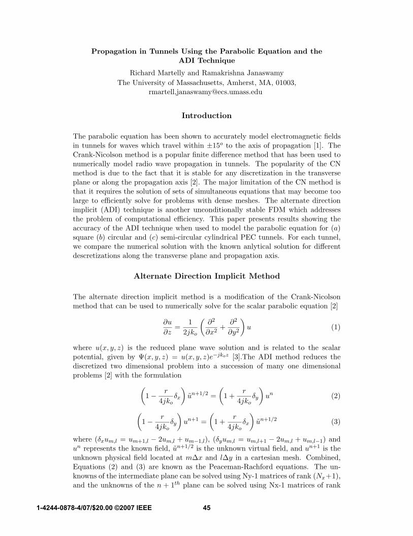
Propagation in Tunnels Using the Parabolic Equation and theADI Technique
Richard Martelly and Ramakrishna JanaswamyThe University of Massachusetts, Amherst, MA, 01003,
rmartell,[email protected]
Introduction
The parabolic equation has been shown to accurately model electromagnetic fieldsin tunnels for waves which travel within ±15o to the axis of propagation [1]. TheCrank-Nicolson method is a popular finite di!erence method that has been used tonumerically model radio wave propagation in tunnels. The popularity of the CNmethod is due to the fact that it is stable for any discretization in the transverseplane or along the propagation axis [2]. The major limitation of the CN method isthat it requires the solution of sets of simultaneous equations that may become toolarge to e"ciently solve for problems with dense meshes. The alternate directionimplicit (ADI) technique is another unconditionally stable FDM which addressesthe problem of computational e"ciency. This paper presents results showing theaccuracy of the ADI technique when used to model the parabolic equation for (a)square (b) circular and (c) semi-circular cylindrical PEC tunnels. For each tunnel,we compare the numerical solution with the known anlytical solution for di!erentdescretizations along the transverse plane and propagation axis.
Alternate Direction Implicit Method
The alternate direction implicit method is a modification of the Crank-Nicolsonmethod that can be used to numerically solve for the scalar parabolic equation [2]
!u
!z=
12jko
!!2
!x2+
!2
!y2
"u (1)
where u(x, y, z) is the reduced plane wave solution and is related to the scalarpotential, given by #(x, y, z) = u(x, y, z)e!jkoz [3].The ADI method reduces thediscretized two dimensional problem into a succession of many one dimensionalproblems [2] with the formulation!
1! r
4jko"x
"un+1/2 =
!1 +
r
4jko"y
"un (2)
!1! r
4jko"y
"un+1 =
!1 +
r
4jko"x
"un+1/2 (3)
where ("xum,l = um+1,l ! 2um,l + um!1,l), ("yum,l = um,l+1 ! 2um,l + um,l!1) andun represents the known field, un+1/2 is the unknown virtual field, and un+1 is theunknown physical field located at m$x and l$y in a cartesian mesh. Combined,Equations (2) and (3) are known as the Peaceman-Rachford equations. The un-knowns of the intermediate plane can be solved using Ny-1 matrices of rank (Nx+1),and the unknowns of the n + 1th plane can be solved using Nx-1 matrices of rank
451-4244-0878-4/07/$20.00 ©2007 IEEE

(Ny + 1). Using the Crank-Nicolson method, the size of the matrix generated willbe (Nx + 1)(Ny + 1) and its elements will not be in tridiagonal or in banded form.As a result, the ADI technique will be more e!cient and solve dense mesh problemsfaster. One di!culty with the ADI technique is that the virtual un+1/2 field hasspecial boundary conditions which may not be the same as the physical boundaryconditions. For our following examples, however, we employ the same boundariesfor the virtual and physical fields.
Waveguide examples using the ADI method
In the following sections, we will use the ADI method to solve for fields in square,circular and semi-circular cylindrical waveguide type tunnels with Dirichlet andNeumann boundary conditions. The waveguides operate at a frequency of 3GHzand have a unit strength gaussian initial field placed at the center with a standarddeviation of 3.5!. The square waveguides have 40! ! 40!(4 ! 4m) cross sectionsand the radius of the circular waveguides are 20!(2m). The distance of propagationfor each example is 1000!(100m). Due to the Nyquist sampling theorem, and thelimitation of the PE, our resolution must be bounded by "x = "y = 2! [4]. Thefigures show pseudocolor plots of the magnitudes of the analytical and numericalscalar potentials for waveguides with Dirichlet and Neumann boundary conditions.The spacings along the transverse plane are "x = "y = 0.4! and the propagationstep size is "z = 10!. Table 1 displays the rms error, defined
Erms =
!1N
"m
"l |uFDM
m,l " uanalm,l |2!
1N
"m
"l |uanal
m,l |2, (4)
where uFDMm,l is the approximated discretized field, uanal
m,l is the known analyticalfield and N is the total number of unknowns. Figures 1 and 2 show good agreementbetween the analytical and numerical fields for the rectangular and circular tunnelswith both Dirichlet and Neumann boundary conditions. For the rectangular tunnel,the Neumann boundary conditions were approximated using 2nd order accurate one-sided approximations and for the circular tunnel, the Neumann boundary conditionswere approximated by first order interior interpolation. In Figure 3, the Neumannboundary condition were approximated with first order one sided approximations.As with the previous two cases, the field patterns are closely matched, however forthe Neumann case the rms error is larger.
Acknowledgments
The authors are pleased to acknowledge the support of the Army Research O!ceunder contract # W911NF-04-1-0028.
Conclusions
The ADI technique for the electromagnetic propagation in PEC waveguides forDirichlet and Neumann boundary conditions is studied and it is found that the field
46

patterns of the numerical solutions are closely matched with that of the analyticalsolutions. Future work will involve the more irregular shapes and mixed boundaryconditions.
References
[1] Alexei V. Popov and Ning Yan Zhu, Modeling Radio Wave Propagation in Tun-nels with a Vectorial Parabolic Equation, IEEE, pp. 1403-1412, September 2000.
[2] John C. Strikwerda, Finite Di!erence Schemes and Partial Di!erential Equations2nd Ed, Philadelphia, PA:Siam, 2004.
[3] Mireille Levy, Parabolic Equation Method for Electromagnetic Wave Propagation,London: Institution of Electrical Engineers, 2000.
[4] Chris A. Zelly, A Three-Dimensional Parabolic Equation Applied to VHF/UHFPropagation over Irregular Terrain, IEEE Trans. Antennas Propagat., 47, pp.1586-1596, October 1999.
Table 1: The normalized rms error.Erms (%) Rectangular WG Circular WG Semi-circular WG
!x,!y !z Dirichlet Neumann Dir. Neu. Dir. Neu.0.8! 5 ! 11.9 10.3 11.4 25.2 12.1 56.40.8! 10 ! 13.7 12.2 13.2 24.2 14.0 55.10.8! 20 ! 19.5 18.0 18.7 21.9 19.7 51.00.4! 5 ! 4.9 4.7 5.0 12.9 5.2 29.10.4! 10 ! 7.3 7.1 7.0 11.9 7.6 27.50.4! 20 ! 14.4 14.2 13.8 12.0 14.6 24.3
Figure 1: The (a) Analytical solution and (b) Numerical approximation of the rect-angular waveguide with Dirichlet boundary conditions (RMS error = 7.3%) and the(c) Analytical solution and (d) Numerical approximation of the rectangular waveg-uide with Neumann boundary conditions (RMS error = 7.1%) .
47

Figure 2: The (a) Analytical solution and (b) Numerical approximation of the cir-cular waveguide with Dirichlet boundary conditions (RMS error = 7.0%) and the(c) Analytical solution and (d) Numerical approximation of the circular waveguidewith Neumann boundary conditions (RMS error = 11.9%).
Figure 3: The (a) Analytical solution and (b) Numerical approximation of the semi-circular waveguide with Dirichlet boundary conditions (RMS error = 7.6%) andthe (c) Analytical solution and (d) Numerical approximation of the semi-circularwaveguide with Neumann boundary conditions (RMS error = 27.5%).
48

Propagation Prediction in Rough and Branched
Tunnels by the ADI-PE Technique (Invited Paper)
R. Martelly! R. Janaswamy†
Abstract — The study of radiowave propagation intunnels is important for the development of telecom-munication systems. The vector Parabolic Equa-tion (PE) and the alternate direction implicit (ADI)technique are used to study radiowave propagationin branched tunnels and in tunnels with rough walls.Previous work has shown that the ADI-PE methodcan accurately predict transmission loss in straighttunnels with smooth walls and with known electricalparameters. We extend the analysis of this methodby including the realistic cases of branching tunnelsand tunnels with rough walls. We breifly discussthe boundary conditions used in each case as well ascompare our results with known numerical or ana-lytical models. The numerical results obtained forthe branched tunnel case were compared with theresults produced by HFSS and the results for therough wall case were compared with known analyt-ical loss factors. The results show excellent agree-ment in both cases.
1 INTRODUCTION
The alternate direction implicit (ADI) method cou-pled with the vector parabolic equation (PE) haspreviously been shown to model radiowave propa-gation in straight tunnels with smooth walls [1, 2].The PE model assumes the propagating fields areslowly varying in the direction of propagation andbackscattered fields are ignored. In realistic tun-nels, over a long distance, higher order propagatingmodes attenuate and the lowest order, slowly vary-ing modes, dominate [3]. The vector PE can ac-curately solve for the lower order dominate modeswhich travel within ± 15o to the axis of propaga-tion.
The vector PE, as formulated by Popov [2], char-acterizes the electrical parameters of the tunnelwalls with an equivalent surface impedance and en-forces the impedance boundary condition [2]. TheCrank-Nicolson method has been traditionally usedto numerically solve the vector PE because it isan unconditionally stable FDM; but it can also becomputationally intensive [1]. The ADI techniqueis also an unconditionally stable implicit FDMthat is significantly more computationally e!cient
!Department of Electrical and Computer Engineering,University of Massachusetts, Amherst, MA, 01003, US, e-mail: [email protected].
†Department of Electrical and Computer Engineering,University of Massachusetts, Amherst, MA, 01003, US, e-mail: [email protected], tel.: 413-545-0937.
than the Crank-Nicolson method [1]. ADI intro-duces slightly more error than the Crank-Nicolsonmethod but previous work has shown that, for mod-est discretizations, the ADI and Crank-Nicolson so-lutions are nearly identical [1]. After a brief discus-sion on the ADI-PE formulization (section 2), wecontinue our analysis of radiowave propagation intunnels using the ADI-PE by considering the spe-cial cases of branched tunnels (section 3) and tun-nels with rough walls (section 4).
2 ADI-PE Theory
The vector PE, as formulated by Popov [2], definesthe transverse electric fields in terms of a vectorfunction, W , as shown in equation (1) [2]
(Ex, Ey)T = We!jkoz, (1)
where ko is the free space wave number and z is thedirection of propagation. The vector function, W ,describes the complex wave amplitude of the planewave. The vector PE can then be defined as
2kojW
!z=
!2W
!x2+
!2W
!y2. (2)
When the impedance boundary condition is en-forced on the tunnel wall, the transverse E fieldsare coupled and the value of W at the boundary isshown to be
W=j
ko
!nx ny
ny !nx
"!1/Zs 0
0 Zs
"!nx ny
ny !nx
"!W
!n. (3)
where nx and ny are the x and y components ofthe normal vector on the boundary and Zs is thenormalized surface impedance.
As shown in [1], the ADI-PE can be summarizedby !
1! rx
4jko"x
"Wn+1/2=
!1 +
ry
4jko"y
"Wn!
1! ry
4jko"y
"Wn+1=
!1 +
rx
4jko"x
"Wn+1/2, (4)
where rx(y) is the mesh ratio and the di"erence quo-tient, "x(y), represent the second order discretiza-tion of the x and y derivatives.
!"#$%$&'&&$((#)$*+,!+-'*.,,/0',,!/1222
596

3 Branched Tunnels
3.1 Branched Tunnel Model
A typical branch tunnel geometry is shown in Fig-ure 1, where the main tunnel axis is shown as asolid bold line and the branch tunnel axis is shownas the long dashed line. The branch angle, !b, is theangle between the axis of the straight and branchtunnel. Using this geometry, the branch angle mustbe less than 30o to ensure that reflected rays enter-ing the branch are within our PE limit of ± 15o.Considering also the rays di!racted from the cor-ners at the junction, we can arrive at a much morestringent requirement of !b < 15. Figures 1 and 2show the incident and reflected ray as it enters thebranch tunnel. The short dashed line markes theinput plane of the branch tunnel. The grazing an-gle, ", and the angle of the ray entering the branch,", are also shown.
Figure 1: The incident and reflected ray enteringthe branch tunnel when " ! !b.
Figure 2: The incident and reflected ray enteringthe branch tunnel when " < !b.
The slope of the branching wall is modeled usinga staircase approximation (see Figure 3a) and theimpedance boundary condition is enforced on allfour walls as outlined in [1] and [2]. The fields alongthe planes marking the entrance of the main tunnel
(line C) and the branch tunnel (line B) are solvedsimultaneously and then used as the initial fields forthe two separate diverging tunnels. We simulate a0.9m"1.0m rectangular tunnel with a branch angleof 15o and operating at a frequency of 900MHz. Weused the far zone field of a unit strength Gaussianfield source as our initial field. The source, withstandard deviation of 0.75#(wavelength), is placedat the center of the tunnel entrance. This means weare only using the lowest order modes as our initialfield [1, 3]. The fundamental mode propagates nearour PE limit at 14.17o.
3.2 Comparison of numerical results toHFSS
For our ADI simulation, we used discretizations(within the tunnel junction) of #x = 0.060 #,#y= 0.054# and #z = 0.013#. The cross-sectionalcoordinates are indicated by x and y, while the ax-ial coordinate in the main tunnel is denoted by thez-axis. To validate our results, we compared our so-lutions with HFSS [6] and plot the magnitude of theEy field along the main and branch tunnel axis. Inthe HFSS simulation, we used radiation boundaryconditions to terminate the tunnel and symmetryplanes to reduce computational labor.
HFSS is a full wave simulator and, unlike theADI-PE, solves for backscattered waves as wellas waves traveling in the forward direction. Thebackscattering is seen as fluctuations in the axialfield in Figure 3b near the diverging tunnels. Thetunnel has a dielectric constant of 5 and conduc-tivity of 0.1 S/m. A high conductivity was chosenso there will be appreciable loss in the small tunneldimensions allowed in HFSS. As we can see fromFigure 3b, there is strong agreement in the axialfield intensity along the main and branch tunnelaxis between the ADI and HFSS. The figure alsoshows that there is about a 10 dB drop when goingfrom the main to the branch tunnel (at the pointmarked C in Figure 3b).
Although the ADI-PE was used to simulatea tunnel with a relatively small electrical cross-section (2.7#"3#), the ADI-PE is capable of han-dling larger tunnels at higher frequencies withoutrunning into memory problems on an average (2 GBRAM) PC [1].
4 Tunnels with Rough walls
4.1 Surface roughness model
Surface roughness is the local variation of the tun-nel wall relative to a mean surface level [4, 5]. Inthis study we consider random surface deviationsin an otherwise smooth wall. For the purpose of
597
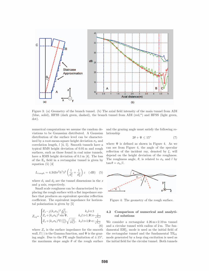
Figure 3: (a) Geometry of the branch tunnel. (b) The axial field intensity of the main tunnel from ADI(blue, solid), HFSS (dark green, dashed), the branch tunnel from ADI (red,*) and HFSS (light green,dot).
numerical computations we assume the random de-viations to be Gauassian distributed. A Gaussiandistribution of the surface level can be character-ized by a root-mean-square height deviation !h andcorrelation length, l [4, 5]. Smooth tunnels have atypical RMS height deviation of 0.01 m and roughsurfaces, such as those found in coal mine tunnels,have a RMS height deviation of 0.1 m [4]. The lossof the Ex field in a rectangular tunnel is given byequation (5) [4]
Lrough = 4.343"2h2#2
!1d41
+1d42
"z ( dB) (5)
where d1 and d2 are the tunnel dimensions in the xand y axis, respectively.
Small scale roughness can be characterized by re-placing the rough surface with a flat impedance sur-face that produces an equivalent specular reflectioncoe!cient. The equivalent impedance for horizon-tal polarization is given by [5]
Zeq=
#$$%$$&Zs!j(ko!h)2
!!
2kol , kol<<1Zs+(ko!h)2 sin ", kol>>1,">> 1!
kol
Zs+(ko!h)2#'
34
() "2j!kol , kol>>1,"<< 1!
kol
(6)where Zs is the surface impedance for the smoothwall, #(·) is the Gamma function, and " is the graz-ing angle. Due to the PE angle limitation of ± 15o,the maximum slope angle $ of the rough surface
and the grazing angle must satisfy the following re-lationship
2$ + " " 15o (7)
where " is defined as shown in Figure 4. As wecan see from Figure 4, the angle of the specularreflection of the incident ray, denoted by %, willdepend on the height deviation of the roughness.The roughness angle, $, is related to !h and l bytan $ = !h/l.
Figure 4: The geometry of the rough surface.
4.2 Comparison of numerical and analyti-cal solutions
We consider a rectangular 4.26m#2.10m tunneland a circular tunnel with radius of 2 m. The fun-damental EHx
11 mode is used as the initial field ofthe rectangular tunnel and the fundamental TE01
mode generated by a loop ring excitation is used asthe initial field for the circular tunnel. Both tunnels
598
operate at a frequency of 1 GHz and the dielectricconstant and conductivity of the tunnel wall aretaken as !r=12 and "o = 0.02 S/m, respectively.
Tables 1 and 2 summarize the mode attenua-tion factors (MAFs), or the loss in dB/km, of thesmooth and rough tunnels with rectangular and cir-cular cross-sections, respectively. In real tunnels, asin our simulations, the lowest order mode will de-termine the MAF over a long distance. We usedequation (5) as our analytical loss factor for boththe rectangular and circular tunnel. As we can seefrom equation (5), the loss due to roughness is afunction of wavelength. To notice an appreciableloss at 1 GHz, we need to assume the walls are asrough as cave walls. Therefore, we used a RMSheight of 0.1 m (0.33#) and a correlation length of2.5m (8.33#) for both tunnels.
The grazing angle of the fundamental mode ofthe rectanglular and circular tunnel is 4.56o and5.25o, respectively. The roughness angle is 2.29o
and equation (7) is satisfied. The ADI is simulatedusing discretizations of !x = 0.284 #, !y = 0.14#and !z = 4 # for the rectangular tunnel and !x =!y =0.44# and !z = 1.67# for the circular tunnel.As we can see from Table 1, the excess loss due toroughness for the rectangular tunnel is about 7 dBwhen using either equation (5) or the ADI-PE. Sim-ilarly, Table 2 shows the same close agreement innumerical and theoretical excess loss for the tunnelwith circular cross-section. In this case, the excessloss due to roughness is about 16 dB.
Rectangular Tunnel ( dB/km)4.26m!2.10 m
Analytical ADI-PEw/o Roughness 31.0 29.5
Roughness 38.0 36.6
Table 1: Analytical and Numerical MAFs.
Circular Tunnel ( dB/km)Radius = 2.0 m
Analytical ADI-PEw/o Roughness 11.0 10.1
Roughness 27.0 26.1
Table 2: Analytical and Numerical MAFs.
The accuracy of the results suggests that theequivalent surface impedance, along with ADI-PE,is an adequate model for determining loss due tosurface roughness. Unlike the ADI-PE, a finite el-ement method would be limited to low frequencies
and electrically small tunnel cross-sections and theequivalent Crank-Nicolson code would require sig-nificantly larger matrices [1].
5 Conclusions
The ADI-PE method has been shown to accu-rately model branch tunnels and tunnels with roughwalls. For branch tunnels, even at the PE limit,there is good agreement between the ADI-PE andwith commerical simulation codes such as HFSS.Also, the additional loss created by tunnels withrough walls is correctly modeled using equivalentimpedances. The ADI-PE method compares wellwith known theoretical roughness loss factors.
Acknowledgments
The authors are pleased to acknowledge the sup-port of the Army Research O"ce under contract #W911NF-04-1-0028.
References
[1] R. Martelly and R. Janaswamy,“An ADI-PEApproach for Modeling Radio TransmissionLoss in Tunnels”, IEEE Transactions on An-tennas and Propagation, 57, 6, June 2009.
[2] A.V. Popov and N.Y. Zhu, “Modeling RadioWave Propagation in Tunnels with a Vecto-rial Parabolic Equation”, IEEE Transactions onAntennas and Propagation, 48, 9, pp. 1403-1412, September 2000.
[3] D.G. Dudley, M. Lienard, S.F. Mahmoud, andP. Degauque, “Wireless Propagation in Tun-nels”, IEEE Antennas and Propagation Mag-azine, 49, 2, pp. 11-26, April 2007.
[4] A.G. Emslie, R.L. Lagace and P.F. Strong,“Theory of the Propagation of UHF RadioWaves in Coal Mine Tunnels”, IEEE Transac-tions on Antennas and Propagation, AP-23,No. 2, pp. 192-205, March 1975.
[5] R. Janaswamy, “Radiowave Propagation andSmart Antennas for Wireless Communica-tions”, New York: Sringer, 2000.
[6] Ansoft Corporation, “User’s Guide: High Fre-quency Structure Simulator V. 9.2”, AnsoftDocumentation, 2003.
599
IOP PUBLISHING JOURNAL OF PHYSICS A: MATHEMATICAL AND THEORETICAL
J. Phys. A: Math. Theor. 41 (2008) 155306 (11pp) doi:10.1088/1751-8113/41/15/155306
Transitional probabilities for the 4-state random walkon a lattice
R Janaswamy
Department of Electrical and Computer Engineering, University of Massachusetts,215-D Marcus Hall, 100 Natural Resources Road, Amherst, MA 01003, USA
E-mail: [email protected]
Received 27 October 2007, in final form 3 March 2008Published 2 April 2008Online at stacks.iop.org/JPhysA/41/155306
AbstractThe diffusion and Schrodinger propagators have been known to coexist on alattice when a particle undergoing random walk is endowed with two states ofspin in addition to the two states of direction in a 1+1 spacetime dimension.In this paper we derive explicit expressions for the various transitionalprobabilities by employing generating functions and transform methods. Thetransitional probabilities are all expressed in terms of a one-dimensional integralinvolving trigonometric functions and/or Chebyshev polynomials of the firstand second kind from which the spacetime continuum limits of the diffusionequation and Schrodinger equation follow directly.
PACS numbers: 03.65.−w, 05.40.Fb
1. Introduction
There has been a lot of interest in the recent past to understand quantum mechanics in thecontext of classical statistical mechanics. On the one hand, Brownian motion provides amicroscopic model of diffusion and provides an unambiguous interpretation of the diffusionequation. On the other hand, a similar physical interpretation is lacking for the Schrodingerequation, whose wave solution is a complex quantity without a physical reality. Becauseclassical diffusion cannot account for the self-interference pattern that is so intrinsic to quantumbehavior, several theories have been put forward recently to understand the microphysics ofquantum behavior. Nelson [1] derived the Schrodinger equation starting from Newtonianmechanics and by assuming that a particle is subject to an underlying Brownian motiondescribed by a combined forward-in-time and a backward-in-time Wiener processes. Adetailed account of Nelson’s original idea of stochastic mechanics and its subsequentrefinement is given in [2–5]. Nottale [6] and Ord [7] advanced the idea that spacetime isnot differentiable but is of a fractal nature, suggesting that an infinity of geodesics lie betweenany two points and, thereby, providing a fundamental and universal origin for the double
1751-8113/08/155306+11$30.00 © 2008 IOP Publishing Ltd Printed in the UK 1

J. Phys. A: Math. Theor. 41 (2008) 155306 R Janaswamy
Wiener process of Nelson. These ideas are elaborated in the monograph [8]. El Naschie [9]too considered a fractal spacetime with a Cantorial structure and argued that quantum behaviorcould be mimicked by combining this fractal spacetime with a diffusion process. A totallydifferent paradigm was recently introduced by Ord [10], who by considering a symmetricrandom walk on a lattice, showed that both the diffusion equation and the Schrodinger equationoccur as approximate descriptions of different aspects of the same classical probabilisticsystem. By considering a 4-state random walk (4RW) on a discrete lattice, wherein a particleis endowed with two states of direction and two states of spin, Ord [10–12] has shown thatboth diffusion and Schrodinger propagators coexist on a lattice and that either can be obtainedfrom a distinct projection of the same random walk. It is too early to speculate as to which ofNelson’s or Ord’s model will duplicate the true quantum behavior under a variety of situations.This can only be ascertained through additional work on both models. It may be mentionedthat the combination of displacement and spin have also been used previously in [13, 14]to study dynamics of a quantum particle in spacetime. However, the important distinctionbetween the Ord model and the one considered in [13, 14] is that the states describing thedirection of motion are independent of those describing the spin states in the former model.There is also an intrinsic notion of memory embedded in the Ord’s model.
The Schrodinger type of equation is encountered under the guise of parabolic waveequation, or simply parabolic equation in the solution of boundary-value problems in severalbranches of applied physics such as acoustics [15], optics and classical electromagnetic wavepropagation [16]. In such boundary-value problems, inhomogeneities of the propagatingmedium caused by the varying index of refraction of the intervening material take the placeof the potential field experienced by a quantum particle. The standard parabolic equationis resulted when one extracts paraxial propagation along a preferred direction from the fullHelmholtz equation. In addition to providing a microscopic model for the Schrodingerequation, the 4RW model considered by Ord is also attractive in the solution of stochasticdifferential equations associated with these parabolic type of equations, carried out byemploying only real random processes. Because walks modeling the Schrodinger equationin the 4RW model traverse only real space, no analytical continuation of boundary data intocomplex space is required that would otherwise be demanded [17, 18] when solving theseboundary-value problems.
Ord does not provide explicit expressions for the various transitional probabilities, but,instead, discusses the continuum limits directly from the governing difference equations. Fora variety of reasons, it is desirable to obtain closed-form expressions (or those involvingintegrals) for these transitional probabilities. In this paper, we provide analytical expressionsfor the transitional probabilities associated with the 4-state random walk in 1+1 dimensionin spacetime by using a transform approach. Our work here is partly motivated by thedesire to have expressions for the transitional probabilities while solving the aforementionedboundary-value problems using the parabolic equation in a homogeneous medium. Usingthese expressions, it is further shown that in the continuum limits as the mesh size shrinks tozero in both space and time, one directly recovers the diffusion equation and the Schrodingerequation. Thus, the main contributions of the paper are to (i) elucidate methodology forobtaining the closed-form expressions for the various transitional probabilities of the 4RW,and (ii) establish the continuum limits of the diffusion and Schrodinger equations describingthe dynamics of particles obeying the 4RW. The methodology presented in this paper ismost suitable for describing quantum dynamics of a free-particle, although the 4RW modelitself has been extended in the presence of a potential field [19]. The paper is organizedas follows: section 2 gives a brief introduction of the random walks considered in [10, 12].Section 3 introduces the generating functions and the 2D transforms considered in this paper.
2

J. Phys. A: Math. Theor. 41 (2008) 155306 R Janaswamy
Table 1. Various states in random walk.
State Direction Spin
1 Right +12 Left +13 Right −14 Left −1
Section 4 provides expressions for the various transitional probabilities as well as discussesthe derivation of the diffusion equation and the Schrodinger equation as continuum limits ofthese probabilities.
2. Multistate random walks
Consider the 4RW model proposed by Ord and Deakin [12], where a particle undergoes randommotion in discrete spacetime (x = m�, t = sε), with x denoting space and t denoting time,and � and ε denoting the spatial and temporal steps, respectively. At every point the particleis endowed with two independent binary properties, its direction of motion (right or left) andits spin or parity (±1). The particle is assumed to change its direction with every collision,but change its spin only every other collision. The four states of the particle correspondingto the four combinations of direction and spin are indicated in table 1. Note that the particlecan execute any direction of motion irrespective of the spin, in contrast to the model used in[13, 14]. However, there is an intrinsic assumption of memory in Ord’s model that arises fromkeeping track of the parity of collisions. If pµ(m�, sε)�,µ = 1, . . . , 4, is the probabilitythat a particle is in state µ at the spacetime point (m�, sε),m = 0,±1,±2, . . . , s = 0, 1, . . . ,
then the transitional relations considered in [12] were of the form
p1[m�, (s + 1)ε)] = αp1[(m − 1)�, sε] + βp4[(m + 1)�, sε]
p2[m�, (s + 1)ε)] = αp2[(m + 1)�, sε] + βp1[(m − 1)�, sε]
p3[m�, (s + 1)ε)] = αp3[(m − 1)�, sε] + βp2[(m + 1)�, sε]
p4[m�, (s + 1)ε)] = αp4[(m + 1)�, sε] + βp3[(m − 1)�, sε],
(1)
where α + β = 1. Here, α is the probability that a particle maintains its direction at the nexttime step, whereas β is the probability that it will change its direction at the next time step.The Markov-chain character of the transitional probabilities is evident from definitions in (1).From the total probability theorem, the probability that a particle is somewhere on the latticeat a given time is equal to 1 and is represented mathematically by
4∑µ=1
∞∑m=−∞
pµ(m�, sε)� = 1. (2)
Ord [10] has shown that the diffusion and Schrodinger propagators coexist on the latticeand that both behaviors are embedded in equations (1). To affect a separation of thediffusive behavior from the wave-like behavior, the following linear transformation isused: q1(m�, sε) = 2s/2[p1(m�, sε) − p3(m�, sε)], q2(m�, sε) = 2s/2[p2(m�, sε) −p4(m�, sε)], w1(m�, sε) = [p1(m�, sε) + p2(m�, sε) + p3(m�, sε) + p4(m�, sε)], andw2(m�, sε) = [p1(m�, sε) + p3(m�, sε)] − [p2(m�, sε) + p4(m�, sε)]. The quantityq1� (without the weight factor 2s/2) indicates the expected difference in the number of
3

J. Phys. A: Math. Theor. 41 (2008) 155306 R Janaswamy
particles of opposite spin arriving at (m�, sε) while moving to the right. Similarly, q2�
refers to the expected number of particles arriving at (m�, sε) while moving to the left.Also, w1(m�, sε)� is the probability that a particle leaves (m�, sε) in either directionand in any spin state, and w2(m�, sε)� is the difference in the probabilities that a particleleaves (m�, sε) to the right and the left. Introducing the shift operator E±1
x pµ(m�, sε) =pµ[(m ± 1)�, sε], a time-advancing operator Etpµ(m�, sε) = pµ[m�, (s + 1)ε], and thevector p = [p1, p2, p3, p4]T , where the superscript T denotes transpose, the transitionalrelations in (1), which are of the form Etp = Sxp, get transformed into
Et
(w1
w2
)= 1
2
( (Ex + E−1
x
) −(Ex − E−1
x
)(α − β)
(Ex − E−1
x
)(α − β)
(Ex + E−1
x
))(
w1
w2
), (3)
Et
(q1
q2
)= 1√
2
(2αE−1
x −2βEx
2βE−1x 2αEx
) (q1
q2
). (4)
Thus the variables (w1, w2) get decoupled from (q1, q2). Essentially, this decoupling resultsfrom block-diagonalizing the matrix Sx and describing the system in terms of its eigenstates.The physical significance of this transformation is touched upon in [11, 12]. Note thatwj and qj need not strictly be probabilistic quantities (meaning �0), but we will continue todescribe them as ‘transitional probabilities’ with the understanding that the actual probabilisticquantities, namely, pµ, can be easily recovered from these using the inverse relations.
3. Generating functions and transforms
We are interested in the solutions of (3) and (4) for the special case of a symmetric randomwalk with α = β = 0.5. In this case we have a set of linear difference equations andthe solution can be obtained conveniently using transform methods [20, 21] and appropriategenerating functions. The key step here is to pick a suitable transform consistent with thenature and domain of definition of the problem. We denote the 2D transform L, consistingof a Fourier transform in space (owing to the unbounded nature of the spatial coordinate) andthe z-transform [22] in time (the z-transform can be arrived from the discretized version of aLaplace transform and is suitable for discrete functions defined on a half-line), of a discretefunction v(m�, sε) as V (kx, z) and define
V (kx, z) = �
∞∑m=−∞
∞∑s=0
v(m�, sε)zs e−imkx� ≡ Lv(m�, sε). (5)
The inverse relation can then be obtained as
v(m�, sε) = 1
4π2i
∫ π/�
kx=−π/�
∮Cz
V (kx, z)
zs+1eimkx� dkx dz ≡ L−1V (kx, z), (6)
where the identities∫ π
kx�=−π
ei(n−m)kx� dkx� = 2πδnm (7)
∮Cz
zr−s−1 dz = 2π iδrs (8)
are used to derive (6). Here δnm is the Kronecker’s delta and Cz is a closed contour around the
origin in the complex z-plane that encloses only the singularities at the origin. The present
4

J. Phys. A: Math. Theor. 41 (2008) 155306 R Janaswamy
analysis, consisting of the z-transform along the time axis and Fourier transform along thespatial axis, is most suitable for studying linear difference equations with constant coefficientssuch as encountered in the study of free-Schrodinger equation by the 4RW model. Othersuitable methods must be devised for studying particle motion in the presence of a potentialfield. Note that V (kx, z) is periodic in kx with a period 2π/�. Using the definition in (5), itcan also be shown that
Lv[m�, (s + 1)ε] = z−1 [V (kx, z) − V0(kx)] (9)
Lv[(m ± 1)�, sε] = e±ikx�V (kx, z), (10)
where V0(kx) is the Fourier transform of the initial distribution v(m�, 0):
V0(kx) = �
∞∑m=−∞
v(m�, 0) e−imkx�. (11)
Note that the periodicity property of V0(kx) implies that V0(π/�) = V0(−π/�).
4. Transitional probabilities
Having defined the required transforms, we will now derive expressions for the transitionalprobabilities w1, w2, q1 and q2. Because of the decoupling afforded in (3) and (4), it issufficient to consider the diffusive and wave-like behaviors separately.
4.1. Diffusive behaviour
The diffusive part of the particle motion is governed by the discrete functions w1 and w2 aswill be evident shortly. Let W1(kx, z) and W2(kx, z) be the 2D transforms of w1(m�, sε) andw2(m�, sε) and ϒ1(kx) and ϒ2(kx) be the transforms of the initial distributions w1(m�, 0)
and w2(m�, 0), respectively. From the definition of w1 in terms of pµ,µ = 1, . . . , 4, andrelation (2), it is seen that ϒ1(0) = 1. On applying the transform L to the set (3) and makinguse of the properties (9) and (10), it is easy to see that W2(kx, z) = ϒ2(kx) and
W1(kx, z) = ϒ1(kx) − iz sin(kx�)ϒ2(kx)
1 − z cos(kx�)(12)
=∞∑
n=0
zn cosn(kx�) [ϒ1(kx) − iz sin(kx�)ϒ2(kx)] (13)
where (13) has been obtained by using the series expansion of [1 − z cos(kx�)]−1. Such aseries converges uniformly provided that |z cos(kx�)| < 1 and this can always be insured bychoosing an appropriate Cz in (6). In other words, the contour Cz is chosen such that thezeroes of the function 1 − z cos(kx�) lie outside it. Substituting this into (6) and making useof (8), we finally arrive at
w1(m�, sε) = 1
2π
∫ π/�
−π/�
coss(kx�)[ϒ1(kx) − i�(s − 1) tan(kx�)ϒ2(kx)] eimkx� dkx, (14)
where �(·) is the Heaviside step function. For a given ϒ1(kx) and ϒ2(kx), integral (14) may becomputed efficiently by the application of the inverse fast Fourier transform (iFFT) algorithm[22]. However, for special values of ϒ1(kx) and ϒ2(kx), the integral may be evaluated in
5
J. Phys. A: Math. Theor. 41 (2008) 155306 R Janaswamy
m
w1(
m∆,
sε)
∆
-20 -15 -10 -5 0 5 10 15 200
0.04
0.08
0.12
0.16
0.2
s = 20s = 30s = 40
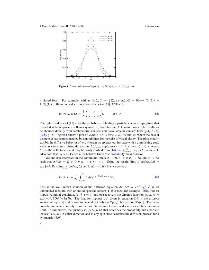
Figure 1. Calculated values of w1(m�, sε) for ϒ1(kx) = 1, ϒ2(kx) = 0.
a closed form. For example, with w1(m�, 0) = 1�
δ0m,w2(m�, 0) = 0(�⇒ ϒ1(kx) =
1, ϒ2(kx) = 0) and m and s even, (14) reduces to ([23], 3.631–17)
w1(m�, sε)� = 1
2s
(s
(s − m)/2
), m � s. (15)
The right-hand side of (15) gives the probability of finding a particle at m in s steps, given thatit started at the origin at s = 0, in a symmetric, discrete-time, 1D random walk. The result canbe obtained directly from combinatorial analysis and is available in standard texts ([24], p 75),([25], p 16). Figure 1 shows a plot of w1(m�, sε)� for s = 20, 30 and 40, where the data atdiscrete m has been connected by smooth lines for the sake of visual clarity. The plots clearlyexhibit the diffusive behavior of w1, wherein w1 spreads out in space with a diminishing peakvalue as s increases. Using the identity
∑∞m=−∞ exp(±imx) = 2πδ(x),−π � x � π , where
δ(·) is the delta function, it may be easily verified from (14) that∑∞
m=−∞ w1(m�, sε)� = 1.Also note that w1 > 0. Hence w1� behaves like a true probability mass function.
We are also interested in the continuum limits � → 0, ε → 0,m → ∞, and s → ∞such that �2/2ε = D > 0,m� → x, sε → t . Using the results lim �→0
s→∞[coss(kx�)] =
exp(−k2
xDt), lim �→0
s→∞[coss(kx�) tan(kx�)] = 0 in (14), we arrive at
w1(x, t) = 1
2π
∫ ∞
−∞ϒ1(kx) e−k2
xDt eikxx dkx. (16)
This is the well-known solution of the diffusion equation ∂w1/∂t = D∂2w1/∂x2 in anunbounded medium with an initial spectral content ϒ1(kx) (see, for example, [26]). For animpulsive initial condition, ϒ1(kx) = 1, and one recovers the Green’s function w1(x, t) =exp(−x2/4Dt)/
√4πDt . The function w1(m�, sε) given in equation (14) is the discrete
version of w1(x, t) and is seen to depend not only on ϒ1(kx), but also on ϒ2(kx). The lattercontribution arises entirely from the discrete nature of space and vanishes in the continuumlimit. To summarize, the quantity w1(m�, sε)� that describes the probability that a particleleaves (m�, sε) in either direction and in any spin state describes the diffusion process for asymmetric 4RW.
6

J. Phys. A: Math. Theor. 41 (2008) 155306 R Janaswamy
4.2. Wave-like behaviour
The wave-like behavior of the particle motion is governed by the discrete functions q1 and q2.The governing equations in this case are repeated below from (4):
Et
(q1
q2
)= 1√
2
(E−1
x −Ex
E−1x Ex
)(q1
q2
). (17)
Our objective here is to derive closed-form expressions for the transitional probabilities q1
and q2. Let Qj(kx, z) be the L transforms of qj (m�, sε), and let j(kx) be the Fouriertransforms of the initial distribution qj (m�, 0), j = 1, 2. On applying the L transform to(17) and making use of properties (9) and (10) and carrying out some algebraic manipulations,we get[
Q1(kx, z)
Q2(kx, z)
]= 1
(1 − √2z cos(kx�) + z2)
[1 − z√
2eikx� − z√
2eikx�
z√2
e−ikx� 1 − z√2
e−ikx�
][1(kx)
2(kx)
]. (18)
To permit evaluation of the integral with respect to z in the inverse transform, we need toexpress Q1 and Q2 in a separable form with respect to kx and z. To this end, we make use ofthe identity ([23], 8.945.2)
1
1 − 2tx + t2=
∞∑0
Un(x)tn, (19)
where Un(·) is the Chebyshev polynomial of the second kind of order n, in (18) to arrive at
Q1(kx, z) =∞∑
n=0
Un
(cos kx�√
2
)zn
[(1 − z√
2eikx�
)1(kx) − z√
2eikx�2(kx)
](20)
Q2(kx, z) =∞∑
n=0
Un
(cos kx�√
2
)zn
[z√2
e−ikx�1(kx) +
(1 − z√
2e−ikx�
)2(kx)
]. (21)
As with the diffusive case, the contour Cz in the inverse transform is chosen such that thezeroes of the denominator function (1 −√
2z cos(kx�) + z2) lie outside it. Equations (20) and(21) may be substituted into the definition of the inverse transform (6) and the integral withrespect to z evaluated by making use of (8). For reasons that will become clear shortly, weare interested in the composite discrete function ψd(m�, sε) = q2(m�, sε) + iq1(m�, sε),which will be compared directly with the solution of the Schrodinger equation. The expressionfor ψd is
ψd(m�, sε) = 1
2π
∫ π/�
−π/�
{Us
(cos kx�√
2
)[2 + i1(kx)]
+ Us−1
(cos kx�√
2
)[(e−iπ/41(kx) − eiπ/42(kx)) cos(kx�)
+ (e−iπ/41(kx) + eiπ/42(kx)) sin(kx�)]
}eimkx� dkx. (22)
As in section 4.1, the integral in (22) may be evaluated efficiently by employing the iFFTalgorithm. In the special case of 1(kx) = 0, 2(kx) = K2, a constant, the expressionprovided in (22) can be further simplified. Making a change of variable y = cos(kx�)
7
J. Phys. A: Math. Theor. 41 (2008) 155306 R Janaswamy
and using dy/√
1 − y2 = −dkx�, cos(m cos−1 y) = Tm(y), where Tm(·) is the Chebyshevpolynomial of the first kind of order m, we can show that
ψd(m�, sε)� = K2
π
∫ 1
−1
1√1 − y2
{Us
(y√2
)Tm(y) − 1√
2Us−1
(y√2
)
× [Tm−1(y) + iTm+1(y)]
}dy. (23)
From the even and odd properties of Chebyshev polynomials, it can be deduced that fors = 2r and m = 2n − 1 (or vice versa), the integral in (23) vanishes implying thatψd [(2n − 1)�, 2rε] = 0 in this special case.
Other interesting identities can be derived starting from (22). Using the relationUs(1/
√2) = Us[cos(π/4)] = sin(sπ/4) + cos(sπ/4), one can readily see that
∞∑m=−∞
ψd(m�, sε)� = e−iπs/4 [2(0) + i1(0)] . (24)
Hence, unlike w1�, the quantities q1� and q2� can be of alternating signs and do not representtrue probability mass functions.
Ord [11] has shown that eight different continuous functions are embedded into thediscrete functions q1 and q2. We will focus on the continuous function that would resultfrom choosing x = 2n�, n = 0,±1,±2, . . . , and t = 8rε, r = 0, 1, 2, . . . , in the discretefunctions q1 and q2. We show that ψd satisfies the Schrodinger equation for m = 2n, s = 8r inthe limit as � → 0, ε → 0, n → ∞, r → ∞ such that �2/2ε = D. The following identities[23, 27] involving Chebyshev polynomials will be utilized in subsequent development:
zUs−1(z) = Us(z) − Ts(z) (25)
d
dzTs(z) = sUs−1(z) (26)
Ts
(1√2
)= cos
(πs
4
), (1 − z2)T ′′
s (z) − zT ′s (z) + s2Ts(z) = 0 (27)
Us−1
(1√2
)=
√2 sin
(πs
4
), (1 − z2)U ′′
s (z) − 3zU ′s(z) + s(s + 2)Us(z) = 0, (28)
where a prime denotes differentiation with respect to the argument. For the purpose ofinvestigating the continuum limits, we would like to cast (22) in a form more suitable forasymptotic analysis. The last term in (22) involving Us−1(·) can be replaced with dTs(·)/dkx
on using the second relation (26) to yieldsin kx�√
2Us−1
(cos kx�√
2
)= −1
s�
d
dkx
Ts
(cos kx�√
2
). (29)
This term is then integrated by parts and simplified using the periodicity condition j (π/�) =j (−π/�), j = 1, 2. A convenient expression for the evaluation of ψd(m�, sε) is thenobtained as
ψd(m�, sε) = 1
2π
∫ π/�
−π/�
eimkx�
{[1(kx) − i2(kx)]Us
(cos kx�√
2
)
+ (1 + i)
([1 + i
m
s
]2(kx) +
[i +
m
s
]1(kx)
)Ts
(cos kx�√
2
)
+1 + i
s�[′
2(kx) − i′1(kx)]Ts
(cos kx�√
2
)}dkx, (30)
8
J. Phys. A: Math. Theor. 41 (2008) 155306 R Janaswamy
which is also more amenable to asymptotic analysis than (22). In the special case of1(kx) = 0, 2(kx) = K2 and for m/s → 0 (small spatial locations and large times) wemove on using (25) that
ψd(m�, sε) = K2
2π
∫ π/�
−π/�
eimkx�
[Ts
(cos kx�√
2
)− i
cos kx�√2
Us−1
(cos kx�√
2
)]dkx. (31)
We now perform an asymptotic analysis for small kx� in (31) and show that ψd(2n�, 8rε)
satisfies the Schrodinger equation. To this end, we note the following Taylor series expansionswhich are obtained by making use of (26)–(28):
cos kx� ∼ 1 − k2x�
2
2+
(kx�)4
4!+ · · · (32)
Ts
(cos kx�√
2
)∼ cos
(πs
4
)− k2
x�2s
2sin
(πs
4
)− (kx�)4s2
4!
×[
3 cos( sπ
4
)− 4
ssin
( sπ
4
)]+ · · · (33)
1√2Us−1
(cos kx�√
2
)∼ sin
(πs
4
)+
k2x�
2s
2
[cos
(πs
4
)− 1
ssin
(πs
4
)]
+(kx�)4
4!
[(10 − 3(s2 − 1)) sin
(πs
4
)− 10s cos
(πs
4
)]+ · · · (34)
Inserting (32)–(34) into (31) and choosing s = 8r,�2 = 2Dε, sε = t, m� = x, s → ∞,
m → ∞,� → 0, ε → 0, we arrive at the desired result:
ψd(x, t) = q2(x, t) + iq1(x, t) ∼ K2
2π
∫ ∞
−∞
(1 − iDk2
xt − k4xD
2t2
2!+ · · ·
)eikxx dkx
= K2
2π
∫ ∞
−∞e−iDk2
x teikxx dkx. (35)
Equation (35) is the spectral representation of the Green’s function corresponding to theSchrodinger equation ∂ψ/∂t = iD∂2ψ/∂x2 with the impulsive initial condition ψ(x, t =0+) = K2δ(x). It has the exact solution
ψ(x, t) = K2√4π iDt
eix2/4Dt . (36)
To reinforce to the reader that the plots of the transitional probabilities (q1, q2) do resemblethe solutions of the free Schrodinger equation, we show in figure 2a comparison of the real,, and imaginary, , parts of the exact solution (36) of the Schrodinger equation with thepartial solution (q1, q2) of the 4RW. The numerical solutions shown in the figure for ψd areon a discrete spacetime (x = m�, t = sε) and have been computed using (31) with theiFFT algorithm [22] with size s = 213 = 8192. It is seen that the 4RW produces solutionsof oscillatory type with both positive and negative excursions for the expectations q1 and q2,which are in excellent agreement with the analytical results for small m
s. This is in contrast to
the quantity w1 shown in figure 1, which, behaving like the solution of the diffusion equation,decays exponentially in space and always remains positive.
9

J. Phys. A: Math. Theor. 41 (2008) 155306 R Janaswamy
m
q 2,R
e(ψ
)
-750 -500 -250 0 250 500 750-0.0075
-0.005
-0.0025
0
0.0025
0.005
0.0075
real [ψ(m∆, sε)]q2(m∆, sε)
s = 8,192, Nfft = 8,192Γ1(kxl) = 0, Γ2(kx) = 0.5m even
m
q 1,Im
(ψ)
-750 -500 -250 0 250 500 750-0.0075
-0.005
-0.0025
0
0.0025
0.005
0.0075
imag [ψ(m∆, sε) ]q1(m∆, sε)
s = 8,192, Nfft = 8,192Γ1 (kx) = 0, Γ2 (kx) = 0.5m even
(a) (b)
Figure 2. Comparison of the exact solution of Schrodinger equation with the discretesolution of a 4RW for an impulsive initial condition. (a) q2(m�, sε), {ψ(m�, sε)} and (b)q1(m�, sε), {ψ(m�, sε)}.
5. Summary
By considering a multistate random walk on a discrete lattice, expressions have been derivedfor the various transitional probabilities using the concept of generating functions. A 2Dtransform involving Fourier transformation in space and the z-transformation in time isemployed to accomplish this. The transitional probabilities governing particle motion areexpressed in terms of integrals involving trigonometric functions in the case of the diffusionequation, and involving Chebyshev polynomials of the first and second kinds in the caseof the Schrodinger equation. Closed-form expressions have been given for particular casesof the initial conditions. The continuum limits of the diffusion equation and Schrodingerequation have been shown to follow directly from these transitional probabilities throughthe performance of appropriate asymptotic analysis. The present analysis consisting of thez-transform along the time axis and Fourier transform along the spatial axis is most suitablefor studying linear difference equations with constant coefficients. In the 4RW model, thiswould correspond to the free Schrodinger equation. The important extension of this analysis tohigher dimensions is worth exploring and would be taken up in the future. The incorporationof a smooth potential field in the Schrodinger equation into the 4RW model has already beenaddressed by Ord in [19] and the study of its transitional probabilities will be taken up in aseparate paper using a different approach.
Acknowledgments
This work was funded in part by the US Army Research Office under ARO grant W911NF-04-1-0228 and by the Center for Advanced Sensor and Communication Antennas, Universityof Massachusetts at Amherst, under the US Air Force Research Laboratory Contract FA8718-04-C-0057.
References
[1] Nelson E 1966 Derivation of the Schrodinger equation from Newtonian mechanics Phys. Rev. 150 1079–85
10

J. Phys. A: Math. Theor. 41 (2008) 155306 R Janaswamy
[2] Nelson E 2001 Dynamical Theories of Brownian Motion 2nd edn (Princeton, NJ: Princeton University Press)web edition at http://www.math.princeton.edu/nelson/books.html
[3] Nelson E 1985 Quantum Fluctuations (Princeton, NJ: Princeton University Press)[4] Nagasawa M 1993 Schrodinger Equations and Diffusion Theory (Boston: Birkhauser)[5] Nagasawa M 2000 Stochastic Processes in Quantum Physics (Boston: Birkhauser Verlag)[6] Nottale L and Schneider J 1984 Fractals and non-standard analysis J. Math. Phys. 25 1296–300[7] Ord G N 1983 Fractal spacetime: a geometric analogue of relativistic quantum mechanics J. Phys. A: Math. Gen.
16 1869–84[8] Nottale L 1995 Scale relativity, fractal space-time and quantum mechanics Quantum Mechanics, Diffusion and
Chaotic Fractals ed M S El Naschie, O E Rossler and I Prigogine (New York: Elsevier)[9] El Naschie M S 1995 Quantum measurement, information, diffusion and cantorian geodesics Quantum
Mechanics, Diffusion and Chaotic Fractals ed M S El Naschie, O E Rossler and I Prigogine (New York:Elsevier Science)
[10] Ord G N 1996 The Schrodinger and diffusion propagators coexisting on a lattice J. Phys. A: Math. Gen.29 L123–8
[11] Ord G N and Deakin A S 1996 Random walks, continuum limits, and Schrodinger’s equation Phys. Rev.A 154 3772–78
[12] Ord G N and Deakin A S 1997 Random walks and Schrodinger’s equation in (2+1) dimensions J. Phys. A:Math. Gen. 30 819–30
[13] Aharonov Y, Davidovich L and Zagury N 1993 Quantum random walks Phys. Rev. A 48 1687–90[14] Aslangul C 2005 Quantum dynamics of a particle with a spin-dependent velocity J. Phys. A: Math. Gen. 38 1–16[15] Jensen F B, Kuperman W A, Porter M B and Schmidt H 1994 Computational Ocean Acoustics (New York:
Springer)[16] Levy M F 2000 Parabolic Equation Methods for Electromagnetic Wave Propagation (London: IEE Press)[17] Budaev B V and Bogy D B 2002 Application of random walk methods to wave propagation Quart. J. Mech.
Appl. Math. 55 206–26[18] Janaswamy R 2007 Solution of BVPs in electrodynamics by stochastic methods IEEE Applied Electromagnetics
Conf. vol 1 (Kolkata, India, 19–20 Dec. 2007)[19] Ord G N 1996 Schrodinger’s equation and discrete random walks in a potential field Ann. Phys. 250 63–8[20] Montroll E W 1965 Random walks on lattices-II J. Math. Phys. 6 167–81[21] Barber M N and Ninham B W 1970 Random and Restricted Walks (New York: Gordan and Breach)[22] Rabiner R R and Gold B 1975 Theory and Application of Digital Signal Processing (Englewood Cliffs, NJ:
Prentice-Hall)[23] Gradshteyn L S and Ryzhik I S 2000 Table of Integrals, Series, and Products 6th edn (New York: Academic)[24] Feller W 1970 An Introduction to Probability Theory and Its Applications vol II 2nd edn (New York: Wiley)[25] van Kampen V G 2007 Stochastic Processes in Physics and Chemistry 3rd edn (New York: North-Holland)[26] Barton G 1989 Elements of Green’s Functions and Propagation (New York: Oxford University Press)[27] Abramowitz M and Stegun I A 1970 Handbook of Mathematical Functions (New York: Dover)
11
IEEE ANTENNAS AND WIRELESS PROPAGATION LETTERS, VOL. 8, 2009 23
Transparent Boundary Condition for the ParabolicEquation Modeled by the 4RW
Ramakrishna Janaswamy, Fellow, IEEE
Abstract—Transparent boundary condition in a 2D-space is pre-sented for the four-state random walk (4RW) model that is usedin treating the standard parabolic equation by stochastic methods.The boundary condition is exact for the discrete 4RW model, isof explicit type, and relates the field in the spectral domain at theboundary point in terms of the field at a previous interior pointvia a spectral transfer function. In the spatial domain, the domainof influence for the boundary condition is directly proportional tothe “time” elapsed. By performing various approximations to thetransfer function, several approximate absorbing boundary condi-tions can be derived that have much more limited domain of influ-ence.
Index Terms—Generating function, parabolic equation, randomwalk, Schrödinger equation, transform methods, transparentboundary condition.
I. INTRODUCTION
P ARABOLIC EQUATION (PE) is used widely in severalareas—including radiowave propagation, underwater
acoustics, fiber optic propagation, etc.—to study propagation ofunidirectional waves in a variety of environments [5], [8], [11].Its form is very similar to the Schrödinger equation in whichthe wavefunction, temporal variable, and the potential take therespective places of the reduced field, the axial coordinate, andthe modified refractive index of the PE. When solving the PE orSchrödinger equation in unbounded regions by differential ordifference equation methods, one has to first restrict the regionto a finite size and simulate an unbounded region by imposingboundary conditions on the truncated domain. If these boundaryconditions exactly simulate an unbounded exterior region as faras the interior problem is concerned, they are termed as exact ortransparent boundary conditions. Transparent boundary condi-tions can be devised for the original partial differential equationor to its discretized version, and this has been done by severalworks in the past: [2], [4], [9], [10], [13], and [1]. ([1] and [4]contain many works outside the traditional electromagnetic areawhere such development took place.) For a number of reasons,there is an interest to treat the PE by stochastic techniques,wherein the desired field is obtained by performing averages
Manuscript received December 08, 2008. First published December 22, 2008;current version published April 17, 2009. This work was supported in part bythe U.S. Army Research Office under ARO Grant W911NF-04-1-0228 and byCASCA, UMass Amherst, under the Air Force Research Laboratory ContractFA8718-04-C-0057.
The author is with the Department of Electrical and Computer Engi-neering, University of Massachusetts, Amherst, MA 01003 USA (e-mail:[email protected]).
Digital Object Identifier 10.1109/LAWP.2008.2011571
over several realizations of Brownian motion or its discretecounterpart of random walk traversing the problem domain[6]. A direct application of stochastic techniques to the PE asdone in [3] necessitates analytical continuation of fields andboundary data, only possible for very limited problems, that ishighly undesirable. The four-state random walk (4RW) model,originally developed by Ord [12] to provide a macroscopicmodel for the Schrödinger equation, alleviates this limitationand results in the same second-order accurate discretizationscheme for the PE as the Crank–Nicolson scheme. Numericalschemes are currently being developed using the 4RW modelto study wireless propagation problems in open domains, andit is the purpose of this letter to derive transparent boundaryconditions for this model by considering 2D propagation in a 1
1-dimensional space. Detailed numerical solutions for prop-agation over terrain and rough surfaces, and in inhomogeneousatmosphere by the 4RW model will be presented in a futurepaper. In the next section, we begin with a brief introductionof the 4RW model, followed by the development of the exactboundary condition.
II. TRANSPARENT BOUNDARY CONDITION FOR 4RW
Consider the standard parabolic equation in the reduced fieldvariable :
(1)
which constitutes a narrow angle approximation to theHelmholtz equation for time-harmonic waves ( timeconvention in the normalized time variable ) with wavenumber
propagating in the - plane, where is the op-erating wavelength and is a complex-valued functionproportional to the modified refractive index (or potentialfor the Schrödinger equation) of the medium. Because thiswork relies heavily on the random walk literature pertainingto the Schrödinger equation, we shall refer to as the “time”coordinate even though it represents the axial space coordi-nate in wave propagation problems. The variable representsthe lateral spatial coordinate and . Presence of thefirst-order derivative in time enables the solution of (1) toproceed with the specification of initial conditions at . Itis assumed that all sources at initial time are confined to theregion (Region I) and that the potential assumes aconstant value for (Region II). Our interestis to derive an artificial boundary condition imposed atfor a discretized version of (1) that simulates free space as far asRegion I is concerned. For simplicity and no loss in generality,we first consider the case of and discuss the solutionfor the nonzero case at the end. For treatment by stochastic
1536-1225/$25.00 © 2009 IEEE

24 IEEE ANTENNAS AND WIRELESS PROPAGATION LETTERS, VOL. 8, 2009
methods, (1) is discretized as per the 4RW model, which,like the Crank-Nicolson finite-difference scheme, results in asecond-order accurate (in space and time) scheme [12]. For aparticle moving on a discrete lattice and subject to random col-lisions, the transitional probabilities in the 4RW at the discretespace–time point are of the form [7], [12]
(2)
where ,, and
, , is the probability that a particle isin state at the space-time point , ,
. The particle changes its direction of motion withevery collision but changes its parity or spin at every othercollision. The combination of two directions of motion and twostates of spin constitutes the four states in the model. It hasbeen shown in [12] that such a 4RW encompasses the diffusionas well as Schrödinger equations and that isthe Schrödinger wave function in the discrete case. The rela-tionship between the temporal and spatial steps of the form
implied in the 4RW model assures the aforemen-tioned second-order accuracy in space. For waves propagatingwithin about the axial direction, the lateral space step isusually restricted to [8], resulting in , valueswhich are consistent with those used in the normal finite-differ-ence or Fourier split-step schemes [8] used to solve the PE.
The operators and in (2) are, respectively, thespatial and temporal advancing operators and are definedmathematically as and
. It is assumed in (2) thatthe random walk is nonpersistent and the probabilities that aparticle maintains or changes its direction at the next time stepare the same. For brevity we will denote as simply
. As in our previous studies, we will assume that thenumber of right-going particles is the same as those going to theleft at time and focus on deriving transparent boundaryconditions for the wave function . The boundary at
separates Region I from Region II and it is furtherassumed for convenience that for .Consider a discrete function and its temporal transform
as defined in [7]
(3)
The quantity may be thought of as the discrete versionof the Laplace transform of . The inverse relation is defined as
(4)
where is a closed contour around the origin in the com-plex -plane that encloses only the singularities at the origin.The symbols and denote the temporal transform and itsinverse respectively. The transformed variable is alsoreferred to as the generating function within the random walkcommunity [14]. If and are two temporal (and
causal) functions with respective generating functionsand , the following shift and convolution properties, re-spectively, can be readily established:
(5)
(6)
Applying the temporal transform to (2) and making use of theshift property (5), and carrying out some algebraic manipula-tions, we arrive at the following equations for the generatingfunction in terms of initial data:
(7)
where is the discrete averaging operator.The right-hand side in (7) is identically zero for Region II, anda knowledge of the general solution in this region permits thederivation of transparent boundary condition. A general solutionof (7) in Region II will be of the form with
constant. The function is then determined from (7) as
(8)
We are interested in the solution that remains bounded for largein Region II, which imposes the condition . Due to
the presence of the radical sign, the function defined by (8) willbe multiple-valued, resulting in two branches of the solution.These two solutions will cross over in the complex plane unlesscare is taken to define each analytically by considering a double-sheeted complex plane. The two sheets intersect at the branchcuts defined by the curve so as to separate the propersolution from the improper one . It ismore illuminating to first study the branch cuts in a transformedcomplex plane , in which the branch pointsoccur at . In the -plane, the branch points occur at
, . With these branch cuts, thetop sheet of the complex -plane is chosen such that
at . A straightforward but tediousanalysis reveals that the branch cut in the -plane is given by thesemicircle , with the real part . The branch cuts inthe - and - planes are shown in Fig. 1. We denote the properbranch by the symbol and the other branch by the symbol
. For the purpose of numerical calculations, one may set. Clearly .
The proper solution in Region II is now given by, which implies that
(9)
Equation (9) is the frequency domain representation of the trans-parent boundary condition that simulates free space for the in-terior region . The function may be interpreted asa transfer function, which relates the input and output functions
and , respectively. For the purpose of numer-ical implementations, it is necessary to prescribe the boundarycondition in the temporal domain. From Fig. 1, it is clear that

JANASWAMY: TRANSPARENT BOUNDARY CONDITION FOR PE MODELED BY 4RW 25
the function is analytic near the origin. The inverse trans-form of involves integration around the closed contour
and is facilitated by performing a Taylor series expansionof near the origin. The infinite series representation of
can then be easily determined as
(10)
where
(11)
Making use of the relation
where is the Kronecker’s delta, we arrive at the corre-sponding temporal function
(12)
Finally, a “time”-domain transparent boundary condition is ob-tained by using the convolution property (6) in (9)
(13)
where is the interger-valued floor function of. Obviously, the summation term will only exist when
. Note that the presence of a term in the series rep-resentation of results in a delayed field inthe temporal representation of the boundary condition. Equation(13), consisting of a finite series, is the exact discrete boundarycondition for terminating the computational domain of the 4RWmodel and is based on an infinite series representation of thetransfer function in a region analytic about the origin. Further-more, it is of explicit type wherein the field at is expressedin terms of the historical field at , . It is alsoseen that the number of terms in (13) will increase linearly with. To reinforce to the reader its accuracy, we place initial sources
, with constantand and compare the exact solution of the field as de-termined from the expressions in [7] with the solutionobtained by substituting the exact solution into the right handside of (13). Note that the earliest “time” at which an impulseplaced initially at will arrive at is .The two solutions plotted in Fig. 2 for are seen to bevirtually on top of each other.
It is possible to derive a hierarchy of approximate boundaryconditions by considering various approximations to thetransfer function . For example, one may perform arational approximation to the function and obtain suc-cessively higher order boundary conditions. A zeroth orderboundary condition is obtained by using and
Fig. 1. Branch cuts in the complex � � � and � planes defining ��� ���� � �.The branch points in the �-plane occur at � � � and � � �� and those in the�-plane at � � � , � � �� � � � � �. Branch cuts are shown as wigglylines.
Fig. 2. True field in unbounded medium and that obtained from (13). (a) Realpart of ���� �. (b) Imaginary part of ���� �.
reads . A better approximation usesand results in the boundary condition
. Approximations

26 IEEE ANTENNAS AND WIRELESS PROPAGATION LETTERS, VOL. 8, 2009
in terms of special functions such as Legendre polynomials arealso possible.
It is straightforward to handle the case with nonzeroby writing the solution of (1) as
, resulting inwith . The boundary condition (9) con-tinues to be valid for the quantity . The spectral domainboundary condition in terms of the actual field becomes
. In the temporal domain we get thecorresponding equation
(14)
Obviously, (14) reduces to (13) for (or ).
III. CONCLUSION
Transparent boundary condition has been presented for the4RW model used to represent a PE in stochastic methods. Theboundary condition, given in the form of a finite series, involvesspecification of the field at a boundary point in terms of the his-torical field at immediate interior points. Several approximateboundary conditions can be derived from it based on a rationalor other approximations to the transfer function.
REFERENCES
[1] A. Arnold, M. Ehrhardt, and I. Sofronov, “Discrete transparentboundary conditions for the Schrödinger equation: Fast calculation,approximation, and stability,” Commun. Math. Sci., vol. 1, no. 3, pp.501–556, 2003.
[2] V. A. Baskakov and A. V. Popov, “Implementation of transparentboundaries for numerical solution of the Schrödinger equation,” WaveMotion, vol. 14, no. 1, pp. 123–128, Jan. 1991.
[3] B. V. Budaev and D. B. B. Bogy, “Application of random walk methodsto wave propagation,” Q. J. Mech. Appl. Math., vol. 55, no. 2, pp.209–226, 2002.
[4] M. Ehrhardt and A. Arnold, “Discrete transparent boundary condi-tions for the Schrödinger equation,” Riv. Mat. Univ. Parma, vol. 6, pp.57–108, 2001.
[5] V. A. Fock, Electromagnetic Diffraction and Propagation Problems.New York: Pergamon Press, 1965.
[6] R. Janaswamy, “Solution of BVPs in electrodynamics by stochasticmethods,” in Proc. IEEE Appl. Electromagn. Conf., Kolkata, India,Dec. 19–20, 2007 [Online]. Available: http://ieeexplore.ieee.org
[7] R. Janaswamy, “Transitional probabilities for the 4-state random walkon a lattice,” J. Phys. A: Math. Theor., vol. 41, Apr. 2008, 155306, (11pp.).
[8] F. B. Jensen, W. A. Kuperman, M. B. Porter, and H. Schmidt, Compu-tational Ocean Acoustics. New York: Springer-Verlag, 1994.
[9] M. F. Levy, “Transparent boundary conditions for parabolic equationsolutions of radiowave propagation problems,” IEEE Trans. AntennasPropag., vol. 45, no. 1, pp. 66–72, Jan. 1997.
[10] S. W. Marcus, “A generalized impedance method for application ofthe parabolic approximation to underwater acoustics,” J. Acoust. Soc.Amer., vol. 90, no. 1, pp. 391–398, Jul. 1991.
[11] K. Okamoto, Fundamentals of Optical Waveguides, 2nd ed. SanDiego, CA: Academic, 2006.
[12] G. N. Ord and A. S. Deakin, “Random walks and Schrödinger’sequation in (2 � 1) dimensions,” J. Phys. A: Math. Gen., vol. 30, pp.819–830, 1997.
[13] J. S. Papadakis, P. Taroudakis, P. J. Papadakis, and B. Mayfield, “Anew method for a realistic treatment of the sea bottom in the parabolicapproximation,” J. Acoust. Soc. Amer., vol. 92, no. 4, pp. 2030–2038,Oct. 1992.
[14] G. H. Weiss, Aspects and Applications of the Random Walk. NewYork: North-Holland, 1994.
IEEE TRANSACTIONS ON ANTENNAS AND PROPAGATION, VOL. 57, NO. 6, JUNE 2009 1759
An ADI-PE Approach for Modeling RadioTransmission Loss in Tunnels
Richard Martelly and Ramakrishna Janaswamy, Fellow, IEEE
Abstract—Alternate direction implicit (ADI) method is usedto study radio wave propagation in tunnels using the parabolicequation (PE). We formulate the ADI technique for use in tunnelswith rectangular, circular and arched cross sections and with lossywalls. The electrical parameters of the lossy walls are charac-terized by an equivalent surface impedance. A vector PE is alsoformulated for use in tunnels with lossy walls. It is shown that theADI is more computationally efficient than the Crank Nicolsonmethod. However, boundary conditions become more difficult tomodel. The boundary conditions of the ADI intermediate planesare given the same boundary conditions as the physical plane andthe overall accuracy is reduced. Also, when implementing the ADIin tunnels with circular cross sections the order at which the lineby line decomposition occurs becomes important. To validate theADI-PE, we show simulation results for tunnel test cases withknown analytical solutions. Furthermore, the ADI-PE is used tosimulate real tunnels in order to compare with experimental data.It is shown that the PE models the electric fields most accuratelyin real tunnels at large distances, where the lower order modesdominate.
Index Terms—Alternate direction implicit (ADI), parabolicequation, radio wave propagation in tunnels.
I. INTRODUCTION
T HE growth of mobile communication systems in recentyears has led to increasing interest in the research of radio
wave propagation in tunnels. The methods that have been tra-ditionally used to model radiowave propagation in tunnels aremodal analysis, geometrical optics and the parabolic equation(PE) approximation.
The modal analysis method and the geometrical opticsmethod both have unacceptable limitations and cannot alwaysbe used to solve for the fields in real tunnels [3]–[5]. The modalapproach uses a simple field representation comprised of onedominate mode and an infinite number of higher order modes.This representation is not always applicable to real tunnelenvironments with arbitrary geometries. Also, it is difficult todetermine eigenfunctions for real tunnels [4]. The geometricaloptics method approximates the field as rays reflected alongthe direct path of propagation. The geometrical optics methodbecomes difficult to use for problems at long range becauseof the large number of reflected waves, and the method fails
Manuscript received March 18, 2008; revised October 20, 2008. Current ver-sion published June 03, 2009. This work was supported by the Army ResearchOffice under Grant ARO W911NF-04-1-0228.
The authors are with the Department of Electrical and Computer Engineering,University of Massachusetts, Amherst, MA 01003 USA (e-mail: [email protected]; [email protected]).
Color versions of one or more of the figures in this paper are available onlineat http://ieeexplore.ieee.org.
Digital Object Identifier 10.1109/TAP.2009.2019891
Fig. 1. Tunnels with (a) rectangular, (b) circular and (c) arched profiles.
completely in caustic regions. By comparison, the standardparabolic equation has been shown to accurately model electro-magnetic fields in tunnels for waves which travel withinto the axis of propagation [2].
Research has been done on the parabolic approximation ofradiowave propagation in tunnels by Popov and Zhu [4] andNoori et al. [5]. The traditional numerical technique used in pre-vious works is the Crank Nicolson method. The popularity ofthe Crank Nicolson method is due to the fact that it is stable forany discretization in the transverse plane or along the propaga-tion axis [2]. The major limitation of the CN method is that itrequires the solution of sets of simultaneous equations that maybecome too large to efficiently solve for problems with densemeshes. The alternate direction implicit (ADI) technique wasdeveloped to address the problem of computational efficiency.The ADI method has been used extensively in previous works tosolve the PE in the form of the heat transfer equation [19]–[22]and in electromagnetics to directly solve Maxwell’s equationusing the FDTD method [23]–[25].
In this paper we use PE together with the ADI technique tostudy transmission loss inside tunnels. In Section II, we showhow the PE can be used to solve for fields in tunnels with per-fectly conducting walls. In this case, we can use a scalar PE andenforce simple Dirichlet or Neumann boundary conditions onthe wall. To model waves in tunnels with lossy walls, we mustuse a vector parabolic equation, as discussed in Section III. Abrief introduction of the CN method is given in Section IV. Asdiscussed in Section V, the ADI maintains the unconditional sta-bility of the CN method while reducing compuational labor. Wedevelop the ADI to deal with straight tunnels with rectangular,circular and arched profiles, as shown in Fig. 1.
For validation purposes, in Section VI, we examine the ac-curacy of the scalar parabolic equation when used to solve forfields in (a) square (b) circular (c) semi-circular cylindrical PECtunnels. Then we examine the accuracy of the vector parabolic
0018-926X/$25.00 © 2009 IEEE

1760 IEEE TRANSACTIONS ON ANTENNAS AND PROPAGATION, VOL. 57, NO. 6, JUNE 2009
equation when used to solve for fields in (d) square and (e) cir-cular cylindrical tunnels with impedance walls in Section VII.Finally, in Section VIII we compare the ADI simulation resultswith published measured data for the case of (f) arched cylin-drical tunnels.
II. SCALAR PARABOLIC EQUATION
The parabolic equation is an approximation of the Helmholtzequation that assumes wave propagation in predominantly onedirection [2]. The PE can be obtained from the Helmholtzequation
(1)
where is either the electric or magnetic scalar potential andis the free space wave number. We choose a solution for the
scalar potential with a fast varying phase term in the directionfactored out
(2)
where is the reduced plane wave solution. The re-duced plane wave is slowly varying along the direction andwe can make the following assumption,
(3)
Physically, the reduced plane wave represents the lower ordermodes which travel predominantly along the -axis. Substi-tuting the plane wave solution into (1), the standard PE follows:
(4)
The PE reduces the 2nd order derivative into a first orderderivative and, as a result, the PE is easier to implement numer-ically using finite differences. As shown in [7], the relative errorepression of the PE can be shown to be
(5)
where the angle is the angle of propagation measured fromthe axis. The level of accuracy will determine the range ofangles over which the PE is valid. For this paper, we adopt thetraditional angle range of . For the angle of 15 the relativeerror is 0.00058. The PE is only valid for waves traveling in thepositive direction at angles within and back scatteredwaves are ignored [2].
In Section VI, we use the PE to solve for fields in PEC waveg-iudes. For these examples, we choose our initial fields so thatonly modes propagating within are significant. The scalarPE can only be used for tunnels with PEC walls. In Section III,we discuss the modifications that must be made to the PE to dealwith tunnels with non-PEC walls.
III. VECTOR PARABOLIC EQUATION
The scalar PE is only valid in cases where the transverse mag-netic and electric fields can propagate independantly of eachother. This is the case when studying perfect electrically con-ducting (PEC) waveguides. If Dirichlet boundary conditions areenforced on the waveguide wall, the propagating field will be ofthe TM type, and if Neumann boundary conditions are enforced,then the field will be of the TE type.
In realistic tunnels, the walls are typically made up of somelossy material such as concrete and rock. The PE approxima-tion has been shown to model realistic tunnels very accuratelyover large distances [4]. This is because higher order modes aremore severely attenuated over large distances due to multiple re-flections. Lower order modes, which propagate at small anglesrelative to the axis, make the most significant contribution to thefield over large distances.
Also, in the case of realistic tunnels, there will exist, in gen-eral, coupling between the TM and TE modes. Unlike the PECcase, we cannot solve the TE and TM modes independently. Wemust now develop a vector PE that will take coupling effectsinto account. Formulation of a vector PE for tunnels with lossywalls and a radius of curvature, , was done by Popov and Zhu[4]. For this paper, we consider only straight tunnels with infi-nite radius of curvature. Although we will not repeat the detailshere, we will briefly discuss the vector PE derivation. In [4], theelectrical parameters on the tunnel walls are approximated bythe Leontovich impedance boundary condition [27]
(6)
where is the outward normal on the tunnel wall and is therelative surface impedance. For a wall with relative permittivity
and conductivity (in S/m), is approximately [18]
(7)
where , , is the complex permittivityand relative conductivity, respectively. Here we use the grazingangle approximation for the surface impedance because the raysthat make the significant contributions to the field at large dis-tances propagate at small angles relative to the axis of propaga-tion.
Starting with normalized Maxwell’s equations
and
(8)where is the intrinsic impedance, is in , is inand is the normalized magnetic field and is in . Wecan define a six component vector
(9)
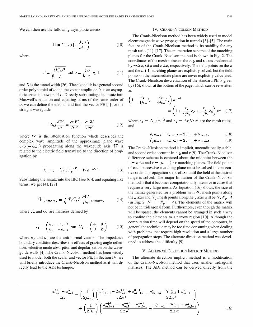
MARTELLY AND JANASWAMY: AN ADI-PE APPROACH FOR MODELING RADIO TRANSMISSION LOSS 1761
We can then use the following asymptotic ansatz
(10)
where
(11)
and is the tunnel width [26]. The eikonal is a general secondorder polynomial of and the vector amplitude is an asymp-totic series in powers of . Directly substituting the ansatz intoMaxwell’s equation and equating terms of the same order of
, we can define the eikonal and find the vector PE [4] for thestraight waveguide
(12)
where is the attenuation function which describes thecomplex wave amplitude of the approximate plane wave
propagating along the waveguide axis. isrelated to the electric field transverse to the direction of prop-agation by
(13)
Substituting the ansatz into the IBC [see (6)], and equating liketerms, we get [4], [28]
(14)
where and are matrices defined by
(15)
where and are the unit normal vectors. The impedanceboundary condition describes the effects of grazing angle reflec-tion, selective mode absorption and depolarization on the wave-guide walls [4]. The Crank–Nicolson method has been widelyused to model both the scalar and vector PE. In Section IV, wewill briefly introduce the Crank–Nicolson method as it will di-rectly lead to the ADI technique.
IV. CRANK–NICOLSON METHOD
The Crank–Nicolson method has been widely used to modelelectromagnetic wave propagation in tunnels [3]–[5]. The mainfeature of the Crank–Nicolson method is its stability for anymesh ratio [11], [17]. The enumeration scheme of the marchingplanes for the Crank–Nicolson method is shown in Fig. 2. Thecoordinates of the mesh points on the , and axes are denotedby , and , respectively. The field points on theand the marching planes are explicitly solved, but the fieldpoints on the intermediate plane are never explicitly calculated.The Crank–Nicolson descretization of the standard PE is givenby (16), shown at the bottom of the page, which can be re-writtenas
(17)
where and are the mesh ratios,and
(18)
(19)
The Crank–Nicolson method is implicit, unconditionally stable,and second order accurate in , and [9]. The Crank–Nicolsondifference scheme is centered about the midpoint between the
and marching planes. The field pointsof each successive marching plane must be solved in consecu-tive order at propagation steps of until the field at the desiredrange is solved. The major limitation of the Crank–Nicolsonmethod is that it becomes computationally intensive in cases thatrequire a very large mesh. As Equation (16) shows, the size ofthe matrix generated for a problem with mesh points alongthe axis and , mesh points along the axis will be(in Fig. 2, ). The elements of the matrix willnot be in tridiagonal form. Furthermore, even though the matrixwill be sparse, the elements cannot be arranged in such a wayto confine the elements to a narrow region [10]. Although thecomputation time will depend on the speed of the computer, ingeneral the technique may be too time consuming when dealingwith problems that require high resolution and a large numberof propagation steps. The alternate direction method was devel-oped to address this difficulty [9].
V. ALTERNATE DIRECTION IMPLICIT METHOD
The alternate direction implicit method is a modificationof the Crank–Nicolson method that uses smaller tridiagonalmatrices. The ADI method can be derived directly from the
(16)

1762 IEEE TRANSACTIONS ON ANTENNAS AND PROPAGATION, VOL. 57, NO. 6, JUNE 2009
Fig. 2. The marching planes of the three-dimensional Crank–Nicolson method.
Crank–Nicolson method by adding to(17)
(20)
where represents the order of error. The error introducedby the new error term is and can be ignored because itis of the same order as the truncation error. Equation (20) abovecan be re-written in factor form
(21)
We can split (21) in a way that allows us to solve for the un-known field line by line (direction by direction)
(22)
(23)
Combined, (22) and (23) are known as the Peaceman–Rachfordmethod [8], [9], [17] and is equivalent to (21) (easily verifiedby multiplying both sides by ). Fig. 3 showsschematics of the line by line decomposition of the planes withinone propagation step. For this example, the unknowns of theintermediate plane can be solved using one matrix and theunknowns of the plane can be solved using one matrix.
One difficulty with the ADI technique, is that it has specialconditions for boundary values in the plane. The andthe planes are physical planes and the intermediate
Fig. 3. The line by line decomposition of the planes using the ADI method.
plane may be considered a virtual plane which may not have thesame boundary conditions as the physical plane. Adding (22)and (23), we arrive at an expression for the intermediate planein terms of the physical planes
(24)
(25)
Equation (24) can only be satisfied if the boundary valuesare known for each propagation step. If we impose the sameboundary conditions on the intermediate plane as the physicalplane, then , and the overallaccuracy will be first order [9]. As with the Crank–Nicolsonmethod, the ADI method is also unconditionally stable [9],[10], [17], [29].
Tunnels with rectangular cross sections are the simplest forADI to handle because one matrix can be used to solve for thefield along the axis and one matrix for the field along theaxis. However, for a circular case, there will need to bematrices to solve for the field along the axis andmatrices to solve for the field along the axis. The Taylor seriesapproximation is used to approximate the curved boundary [10]and different ADI matrices must be used for each line. The sizeof the matrices will depend on the number of mesh points alonga line of the circle.
Another complication arises when enforcing Neumann-typeboundary conditions. Using the technique outlined in Morton[10], we can derive a first order normal derivative using interpo-lation in order to express boundary mesh points in terms of inte-rior mesh points. As a result, the Neumann boundary conditionmay couple two lines in one dimension and increase our numberof unknowns. This makes the order in which the line by line de-composition occurs important. For a circle, the line by line de-composition must begin at the center line where the boundaryvalues are reflected inward and there is no coupling. This makesthe complete solution of the center line possible without the in-troduction of new unknowns. The lines directly adjacent to thecenter line must be solved next and so on until the field alongthe plane is solved completely. In order to avoid increasing thenumber of unknowns and the size of the ADI matrices, the linesmust be solved in successive order.
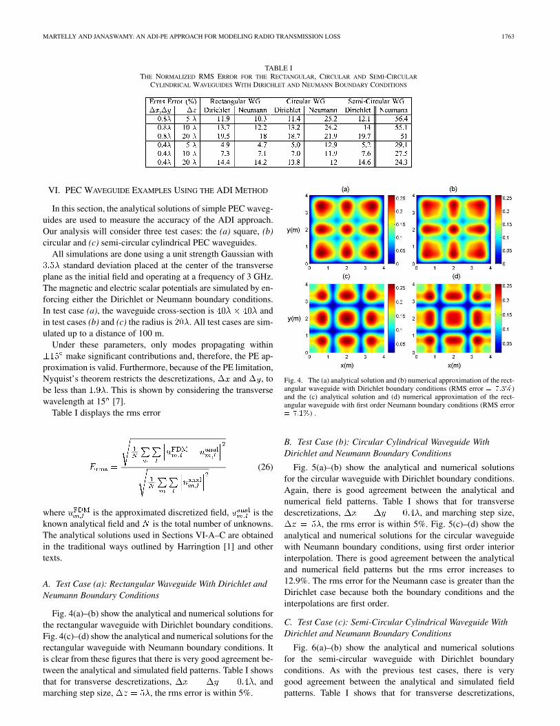
MARTELLY AND JANASWAMY: AN ADI-PE APPROACH FOR MODELING RADIO TRANSMISSION LOSS 1763
TABLE ITHE NORMALIZED RMS ERROR FOR THE RECTANGULAR, CIRCULAR AND SEMI-CIRCULAR
CYLINDRICAL WAVEGUIDES WITH DIRICHLET AND NEUMANN BOUNDARY CONDITIONS
VI. PEC WAVEGUIDE EXAMPLES USING THE ADI METHOD
In this section, the analytical solutions of simple PEC waveg-uides are used to measure the accuracy of the ADI approach.Our analysis will consider three test cases: the (a) square, (b)circular and (c) semi-circular cylindrical PEC waveguides.
All simulations are done using a unit strength Gaussian withstandard deviation placed at the center of the transverse
plane as the initial field and operating at a frequency of 3 GHz.The magnetic and electric scalar potentials are simulated by en-forcing either the Dirichlet or Neumann boundary conditions.In test case (a), the waveguide cross-section is andin test cases (b) and (c) the radius is . All test cases are sim-ulated up to a distance of 100 m.
Under these parameters, only modes propagating withinmake significant contributions and, therefore, the PE ap-
proximation is valid. Furthermore, because of the PE limitation,Nyquist’s theorem restricts the descretizations, and , tobe less than . This is shown by considering the transversewavelength at 15 [7].
Table I displays the rms error
(26)
where is the approximated discretized field, is theknown analytical field and is the total number of unknowns.The analytical solutions used in Sections VI-A–C are obtainedin the traditional ways outlined by Harringtion [1] and othertexts.
A. Test Case (a): Rectangular Waveguide With Dirichlet andNeumann Boundary Conditions
Fig. 4(a)–(b) show the analytical and numerical solutions forthe rectangular waveguide with Dirichlet boundary conditions.Fig. 4(c)–(d) show the analytical and numerical solutions for therectangular waveguide with Neumann boundary conditions. Itis clear from these figures that there is very good agreement be-tween the analytical and simulated field patterns. Table I showsthat for transverse descretizations, , andmarching step size, , the rms error is within 5%.
Fig. 4. The (a) analytical solution and (b) numerical approximation of the rect-angular waveguide with Dirichlet boundary conditions (RMS error � ����)and the (c) analytical solution and (d) numerical approximation of the rect-angular waveguide with first order Neumann boundary conditions (RMS error� ����) .
B. Test Case (b): Circular Cylindrical Waveguide WithDirichlet and Neumann Boundary Conditions
Fig. 5(a)–(b) show the analytical and numerical solutionsfor the circular waveguide with Dirichlet boundary conditions.Again, there is good agreement between the analytical andnumerical field patterns. Table I shows that for transversedescretizations, , and marching step size,
, the rms error is within 5%. Fig. 5(c)–(d) show theanalytical and numerical solutions for the circular waveguidewith Neumann boundary conditions, using first order interiorinterpolation. There is good agreement between the analyticaland numerical field patterns but the rms error increases to12.9%. The rms error for the Neumann case is greater than theDirichlet case because both the boundary conditions and theinterpolations are first order.
C. Test Case (c): Semi-Circular Cylindrical Waveguide WithDirichlet and Neumann Boundary Conditions
Fig. 6(a)–(b) show the analytical and numerical solutionsfor the semi-circular waveguide with Dirichlet boundaryconditions. As with the previous test cases, there is verygood agreement between the analytical and simulated fieldpatterns. Table I shows that for transverse descretizations,

1764 IEEE TRANSACTIONS ON ANTENNAS AND PROPAGATION, VOL. 57, NO. 6, JUNE 2009
Fig. 5. The (a) analytical solution and (b) numerical approximation of the cir-cular waveguide with Dirichlet boundary conditions (RMS error � ����) andthe (c) analytical solution and (d) numerical approximation of the circular wave-guide with Neumann boundary conditions (RMS error � ������).
Fig. 6. The (a) analytical solution and (b) numerical approximation of the semi-circular waveguide with Dirichlet boundary conditions (RMS error � ����)and the (c) analytical solution and (d) numerical approximation of the semi-circular waveguide with Neumann boundary conditions (RMS error� ����).
, and marching step size, , the rmserror is about 5.2%.
Fig. 6(c)–(d) show the analytical and numerical solutions forthe semi-circular waveguide with Neumann boundary condi-tions. There is very good agreement between the field patternsin both cases. However, Table I shows forand , the rms error is very large (29%). Fig. 7 showsthe analytical (solid-line) and simulated (dashed-line) fields at
. As shown in the figure, the error is concentrated nearand the field pattern is preserved. Like in the circular
Neumann case, the rms error can be improved by decreasingthe mesh descretizations. Also, we can see from Table I the errorgrows slightly as the step size is decreased with fixed mesh de-scretizations. This is because the field is converging towards afield not exactly matching the analytical solution.
Fig. 7. The magnitude of the analytical (blue, solid) and simulated (red,dashed) field at � � � for PEC tunnel with semi-circular cross-section andNeumann boundary conditions.
Although the ADI method can produce larger errors than theCN method, for the examples considered, the fields generatedby both codes are nearly identical. Keeping the descretizationsthe same, the error between the two methods is less than 1%. Adiscussion on the accuracy of the ADI method can be found in[30].
VII. IMPEDANCE WAVEGUIDE EXAMPLES
USING THE ADI METHOD
Tunnels with impedance walls can be very difficult to solveand, aside from some special cases, closed form solutions maynot exist [6], [14]. In Sections VII-A and B, we will considerlossy tunnels with known analytical solutions. We will con-sider two such cases, the rectangular tunnel with small surfaceimpedance and the circular tunnel with a linear dipole locatedat its center.
A. Rectangular Tunnel
Exact analytical solutions for the fields in rectangular tunnelswith lossy walls do not exist [6], [14]. In [6], a lossy tunnel istreated as an imperfect metal waveguide with the relative surfaceimpedance of a good conductor
(27)
If the magnitude of the relative surface impedance is much lessthan unity, then perturbation techniques can be used to deriveapproximate fields [6]. Unlike the perfect waveguide case, pureTE and TM modes will not always propagate within the im-perfect waveguide. Instead, there will exist hybridand modes that are coupled TE and TM modes. The
mode is a TE mode with a small TM component,and the mode is a TM mode with a small TE com-ponent.
In the case of the rectangular tunnel, the impedance matrix, shown in (15), becomes diagonal because the normal
vectors, and , disappear alternatively on the tunnel wall.Therefore, the transverse reduced field componentsand in the orthogonal plane are decoupledand can be solved independently [4]. The hybrid fields that aresolved numerically will depend on the boundary conditionsenforced on the waveguide walls.

MARTELLY AND JANASWAMY: AN ADI-PE APPROACH FOR MODELING RADIO TRANSMISSION LOSS 1765
Fig. 8. Rectangular waveguide profiles displaying the boundary conditions forthe � field of the�� mode and the � field of the� � mode in the trans-verse plane.
Consider the simple example of a rectangular waveguide, , with three PEC walls and one impedance
wall located at , where the normal vectors are and. Fig. 8 shows the boundary conditions at the three PEC
walls for the [Fig. 8(a)] and the [Fig. 8(b)] hybridmodes with the and fields given by [6, Eq. (36)].
Let us consider the case of the mode propagatingin the waveguide at a frequency of 1 GHz with a wall ofimpedance, . Good conductors have largeconductivity, and for this case the equivalent conductivityis 556 S/m. Fig. 9(a) shows the magnitude of the analyticalsolution of in the origin plane of and Fig. 9(b)shows the magnitude of the analytical solution of at thedistance of . Fig. 9(c) shows the magnitude of thesimulated , using the analytical field in the origin planeas the initial field. The discretizations along the transverseplane are , and along the propagationaxis, . We can see that there is strong agreementbetween the analytical field and the simulated field in thetransverse plane. The field pattern doesn’t depend on distancebecause a single mode was used as the initial field. The ADIsimulation produced the same pattern throughout the step bystep simulation. For this case, this difference between the modeattenuation factors (MAFs) of the analytical and numericalsolution is 2.36 dB/km.
Now, let us consider the case of the mode propa-gating in the waveguide at a frequency of 1 GHz with a wallof impedance, . For this case the equivalentconductivity is 0.62 S/m. Fig. 9(d) shows the magnitude of theanalytical solution of in the origin plane of . Fig. 9(e)shows the magnitude of the analytical solution of at the axialdistance of . The distance of 5 km was chosen so thatthere would be noticeable attenuation along the axial direction.Fig. 9(f) shows the magnitude of the simulated field, usingthe analytical field in the origin plane as the initial field. Thediscretizations along the transverse plane are the same as in the
example, and . Again,as in the example, we can see that there is strong agree-ment between the analytical and the simulated field patterns inthe transverse plane. Also, the magnitudes of the analytical andsimulated fields show that the simulated field captures the atten-uation of the field along the direction.
Fig. 9. The magnitudes of the analytical and numerical fields of the(a–c) �� and (d–f) � � mode.
Fig. 10. Cross-section of a circular tunnel with lossy walls and a linear sourcelocated at the center.
The main advantage of the ADI method over theCrank–Nicolson method is the use of smaller ADI matrices. Inthe rectangular case, and fields are decoupled and eachfield can be treated as a scalar PE problem. As with the previousscalar PE problems, if there are and mesh points alongthe and dimensions, respectively, the Crank–Nicolsonmatrix will be a sparse matrix of rank . However,the ADI method will only require 2 matrices of rank and
, respectively.
B. Circular Tunnel
Next, we use the ADI-PE to solve for the field in a lossy tunnelwith a circular cross-section of radius (shown in Fig. 10). Thetunnel is treated as a hole in a lossy dielectric medium wherethe interior is free space and the exterior is characterized by
, with . Fig. 10 also shows the lineardipole current source with dipole moment P (in amp-meters),
, located at the center of the tunnelin the plane. The derivation of the electric
fields produced by this source is well known and the details aregiven in [14] and [15].
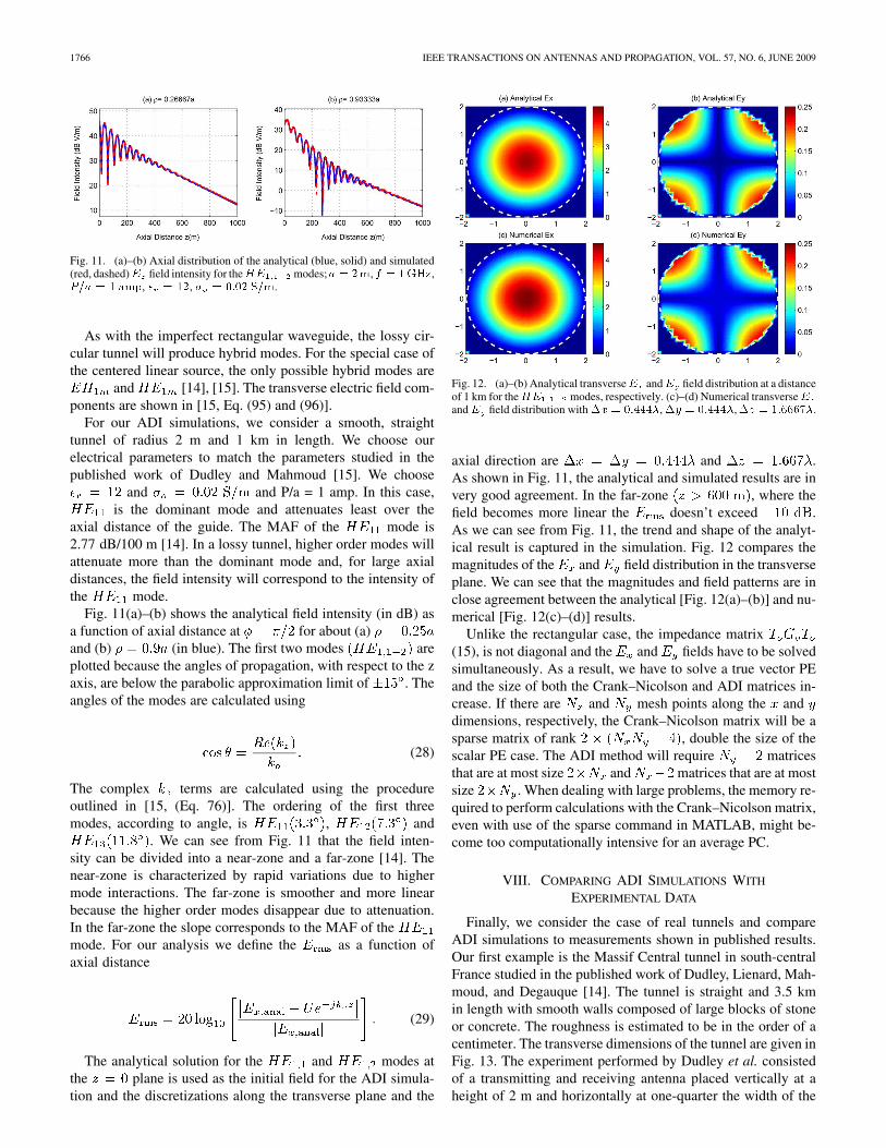
1766 IEEE TRANSACTIONS ON ANTENNAS AND PROPAGATION, VOL. 57, NO. 6, JUNE 2009
Fig. 11. (a)–(b) Axial distribution of the analytical (blue, solid) and simulated(red, dashed)� field intensity for the�� modes;� � ��, � � ����,��� � � ��, � � ��, � � � ���.
As with the imperfect rectangular waveguide, the lossy cir-cular tunnel will produce hybrid modes. For the special case ofthe centered linear source, the only possible hybrid modes are
and [14], [15]. The transverse electric field com-ponents are shown in [15, Eq. (95) and (96)].
For our ADI simulations, we consider a smooth, straighttunnel of radius 2 m and 1 km in length. We choose ourelectrical parameters to match the parameters studied in thepublished work of Dudley and Mahmoud [15]. We choose
and and P/a = 1 amp. In this case,is the dominant mode and attenuates least over the
axial distance of the guide. The MAF of the mode is2.77 dB/100 m [14]. In a lossy tunnel, higher order modes willattenuate more than the dominant mode and, for large axialdistances, the field intensity will correspond to the intensity ofthe mode.
Fig. 11(a)–(b) shows the analytical field intensity (in dB) asa function of axial distance at for about (a)and (b) (in blue). The first two modes areplotted because the angles of propagation, with respect to the zaxis, are below the parabolic approximation limit of . Theangles of the modes are calculated using
(28)
The complex terms are calculated using the procedureoutlined in [15, (Eq. 76)]. The ordering of the first threemodes, according to angle, is , and
. We can see from Fig. 11 that the field inten-sity can be divided into a near-zone and a far-zone [14]. Thenear-zone is characterized by rapid variations due to highermode interactions. The far-zone is smoother and more linearbecause the higher order modes disappear due to attenuation.In the far-zone the slope corresponds to the MAF of themode. For our analysis we define the as a function ofaxial distance
(29)
The analytical solution for the and modes atthe plane is used as the initial field for the ADI simula-tion and the discretizations along the transverse plane and the
Fig. 12. (a)–(b) Analytical transverse� and� field distribution at a distanceof 1 km for the�� modes, respectively. (c)–(d) Numerical transverse�and � field distribution with � � �,�� � �,� � ������.
axial direction are and .As shown in Fig. 11, the analytical and simulated results are invery good agreement. In the far-zone , where thefield becomes more linear the doesn’t exceed .As we can see from Fig. 11, the trend and shape of the analyt-ical result is captured in the simulation. Fig. 12 compares themagnitudes of the and field distribution in the transverseplane. We can see that the magnitudes and field patterns are inclose agreement between the analytical [Fig. 12(a)–(b)] and nu-merical [Fig. 12(c)–(d)] results.
Unlike the rectangular case, the impedance matrix(15), is not diagonal and the and fields have to be solvedsimultaneously. As a result, we have to solve a true vector PEand the size of both the Crank–Nicolson and ADI matrices in-crease. If there are and mesh points along the anddimensions, respectively, the Crank–Nicolson matrix will be asparse matrix of rank , double the size of thescalar PE case. The ADI method will require matricesthat are at most size and matrices that are at mostsize . When dealing with large problems, the memory re-quired to perform calculations with the Crank–Nicolson matrix,even with use of the sparse command in MATLAB, might be-come too computationally intensive for an average PC.
VIII. COMPARING ADI SIMULATIONS WITH
EXPERIMENTAL DATA
Finally, we consider the case of real tunnels and compareADI simulations to measurements shown in published results.Our first example is the Massif Central tunnel in south-centralFrance studied in the published work of Dudley, Lienard, Mah-moud, and Degauque [14]. The tunnel is straight and 3.5 kmin length with smooth walls composed of large blocks of stoneor concrete. The roughness is estimated to be in the order of acentimeter. The transverse dimensions of the tunnel are given inFig. 13. The experiment performed by Dudley et al. consistedof a transmitting and receiving antenna placed vertically at aheight of 2 m and horizontally at one-quarter the width of the

MARTELLY AND JANASWAMY: AN ADI-PE APPROACH FOR MODELING RADIO TRANSMISSION LOSS 1767
Fig. 13. The profile of the Massif Central tunnel.
tunnel , shown as an “ ” in Fig. 13. The trans-mitting power was 34 dBm and the frequencies of 450 MHzand 900 MHz are studied. Half-wave vertical dipoles are usedfor 450 MHz,and vertically polarized wide-band horn antennas(with a gain of 7 dBi) are used for 900 MHz.
The research team of Dudley et al. [14] uses an equivalentrectangular tunnel (see Fig. 13) in order to characterize theMassif Central tunnel. The dimensions of the rectangular tunnelare shown in Fig. 13 and the electrical parameters are chosento be and . The theoretical attenuationconstant of the dominant mode of the equivalent rectangulartunnel is given by [13] and [14]
(30)
where is the horizontal length and is the vertical length,given by and . The attenuation ofthe dominate mode in the equivalent rectangular tunnel corre-sponds to the attenuation of the measured field in the MassifCentral tunnel. Figs. 14 and 15 show the field intensity in dBmas a function of axial distance (in blue) as measured by the re-search team of Dudley et al. [14]. The MAF of the equivalentrectangular tunnel and the experimental data are shown in thefirst two rows of Table II.
The ADI simulations are done using the actual arched cross-section of the Massif Central tunnel and the equivalent rectan-gular tunnel (Fig. 13). The electrical parameters are chosen tomatch the parameters of the research team. At this point, it isimportant to discuss possible sources of error in the simulationof real tunnels. One possible error may be the incorrect predic-tion of electrical parameters of the tunnel walls. If a real tunnelis made up of dry cement and stone, the parameters will dependon the materials used to mix the cement and its percentage ofwater content. One source estimates the parameters of dry con-crete to vary from andand for wet concrete, and[16]. In addition, the electrical parameters will also change withfrequency. For the equivalent rectangle, this isn’t a problem be-cause the parameters have been fixed in [14].
The initial field used in the simulations may not represent theactual antenna field used in measurements. However, even withan incorrect initial field, the field in the far zone, where lower
Fig. 14. The electric-field intensity in dBm and the corresponding least squarefit line of the (a) Massif Central tunnel (blue, solid), (b) the ADI solution usingthe equivalent rectangular profile with � � � and � � ���� ��� (red,dashed), (c) the ADI solution using the arched profile with � � � and � �
���� ��� (green, circle) and (d) the ADI solution using the arched profile with� � �� and � � ���� ��� (black, asterisk) as a function of axial distanceand operating frequency of 450 MHz.
Fig. 15. The electric-field intensity in dBm and the corresponding least squarefit line of the (a) Massif Central tunnel (blue, solid), (b) the ADI solution usingthe equivalent rectangular profile with � � � and � � ���� ��� (red,dashed), and (c) the ADI solution using the arched profile with � � � and� � ���� ��� (green, circle) as a function of axial distance and operatingfrequency of 900 MHz.
order modes dominate, the correct attenuation will be obtained.This allows us some flexibility when setting up our simulations.So long as the lower order modes are illuminated, different ini-tial fields will yield the same MAFs in the far zone. This dis-crepancy is accounted for by offsetting the vertical axis of thesimulation data so the least square fitted lines intersect at thefar zone point. Instead of having the dipole inside the tunnel en-trance, as in the Massif Central experiment, we set up the dipole30 m away from the tunnel opening. This allows us to use thefar field expressions for the dipole and avoid solving more com-plicated field patterns. We do not know the value of the fieldalong the boundary wall in the initial plane. If we use the free

1768 IEEE TRANSACTIONS ON ANTENNAS AND PROPAGATION, VOL. 57, NO. 6, JUNE 2009
TABLE IITHE EXPERIMENTAL, THEORETICAL AND SIMULATED MODE ATTENUATION
FACTORS FOR THE MASSIF CENTRAL TUNNEL
space values along the boundary, the error will be in the form ofhigh oscillations in the MAFs in the far zone. We can eliminatethese oscillations by filtering off the field at the boundary witha unit gaussian with (450 MHz) and(900 MHz). We don’t expect an exact match between the simu-lated results and the measured results in the near zone where theparabolic approximation is not satisfied. However, we expect, inthe far-zone, the E-field and the field attenuation to be correctlymodeled by the simulation. Figs. 14–15 show the simulated fieldintensity in dBm of the tunnel with an arched cross section (ingreen, circle) and the equivalent rectangle (in red, dashed). TheMAFs of the simulations are computed from the slope of theleast square fit line using data in the far zone. The MAFs of thesimulations and the far zone ranges are shown in Table II.
In Fig. 14, for the 450 MHz case, we can see that there isgood agreement between the simulated rectangular tunnel andthe measured data. Table II shows the discrepancies of the MAFsof the measured data, the equivalent rectangle and the simu-lated rectangle are about 2 dB/km. The discrepancy of the sim-ulated results for the arched shape tunnel and the measured datais about 11 dB/km. This is believed to be the result of usingan incorrect electrical parameter. Increasing the magnitude ofthe electrical parameters for the arched shape will increase theattenuation of the tunnel. This is shown in Fig. 14, where theblack curve is the simulation for and .In Fig. 15, for the 900 MHz case, we see that there is moreagreement among all the simulations. As Table II shows, the dis-crepancies among all the simulations are within 1 dB/km. Thegood agreement may be due to the frequency dependant natureof the electrical parameters. At 900 MHz, the electrical parame-ters used for the equivalent rectangle may be in better agreementwith the actual electrical parameters of the tunnel wall.
Our second example is a railway tunnel in Japan studied in thepublished work of Chiba, Inaba, Kuwamoto, Banno, and Sato[12]. The tunnel is straight and 1.47 km in length and also madeup of concrete. The cross-section of the tunnel is arched shapedand has two 3.9 m lanes separated by a notch. Fig. 16 showsthe dimensions of the tunnel cross-section. The measurementteam used half-wave dipole antennas for the transmitters and re-ceivers and the antennas were placed at a height of 3.6 m abovethe ground and 30 m from the tunnel opening with a transmitting
Fig. 16. The profiles of the (a) Japanese National Railway tunnel and (b) theequivalent circular tunnel.
Fig. 17. The (a) MAF of the Japanese National Railway tunnel (blue, solid), (b)the electric-field intensity and least square fit line of the ADI solution using theequivalent circular profile (red, asterisk) and (c) the electric-field intensity andleast square fit line of the ADI solution using the arched profile (green, circle)as a function of axial distance with an operating frequency of 470 MHz.
power of 1 W. The measurement team characterized the tunnelwith an equivalent area circular cylindrical waveguide of radius4.2 m. The electrical parameters of the equivalent circular cylin-drical tunnel were chosen so that the attenuation of the dominantmode will correspond to the attenuation of the measured field.The theoretical attenuation constant is given by (31), shown atthe bottom of the page, where is the root of the thBessel function. The MAF of the equivalent circular cylindricaltunnel is defined, and . Figs. 17 and 18show the theoretical MAF of the dominant mode of the equiva-lent circular cylindrical tunnel (blue).
The ADI simulations are done using the arched shape crosssection (Fig. 16) and the equivalent circular cross section. As
(31)

MARTELLY AND JANASWAMY: AN ADI-PE APPROACH FOR MODELING RADIO TRANSMISSION LOSS 1769
Fig. 18. The (a) MAF of the Japanese National Railway tunnel (blue, solid),(b) the electric-field intensity and least square fit line of the ADI solution usingthe equivalent circular profile (red, asterisk) and (c) the electric-field intensityand least square fit line of the ADI solution using the arched profile (green,circle) as a function of axial distance with an operating frequency of 900 MHz.
TABLE IIITHE EXPERIMENTAL, THEORETICAL AND SIMULATED MODE
ATTENUATION FACTORS FOR THE RAILWAY TUNNEL
before, the electrical parameters are chosen to match the pa-rameters of the research team. Figs. 17 and 18 show the sim-ulated field intensity of the tunnel with an arched cross-section(in green, circle) and the equivalent circle (in red, asterisk). Thefield intensity is shown in dB such that .
In Fig. 17, for the 470 MHz case, we can see that there isreasonable agreement between the attenuation of the simulatedequivalent circular cylindrical tunnel and the theoretical atten-uation. As with the previous tunnel, the simulation is least ac-curate in this frequency range. As we increase the frequencythere is greater agreement between the theoretical MAF and thesimulated fields. As before, we can see from the figures that inthe 470 MHz and 900 MHz cases, the two mode interactions arepresent in the far zone [14]. Table III summarizes the theoreticalMAF, the simulated equivalent circular cylindrical tunnel andthe tunnel with an arched cross section MAFs. The discrepancybetween the theoretical MAF and the equivalent circular cylin-drical tunnel is about 1 dB/km and lower for both frequencies.The discrepancy between the theoretical MAF and the tunnelwith arched cross section about 6.5 dB/km for 470 MHz and3.3 dB/km for 900 MHz.
A. Usage of CPU Time and Memory
In this section, we briefly examine the computation timeand memory usage of the Crank–Nicolson and ADI method.Table IV shows a side by side comparison of the execution timeand CPU memory of the Crank–Nicolson and ADI method
TABLE IVTHE CPU MEMORY AND COMPUTATIONAL TIME FOR � � �� AND
2000 MARCHING STEPS FOR THE TUNNEL WITH RECTANGULAR
PROFILE AND DIRICHLET BOUNDARY CONDITIONS
for the case of a PEC tunnel with a rectangular profile withresolution and using 2000 marching steps.The execution time refers to the time it take MATLAB toperform the one Backslash command and multiplied by thenumber of loops. This accounts for any variation in codes byonly recording the time it takes to invert the matrices. Forthe Crank–Nicolson method, the Backslash command wasperformed after the memory saving Sparse command was used.As we can see from Table IV, ADI runs mush faster and takessignificantly less memory than the Crank–Nicolson method.
To continue the comparison between the Crank–Nicolsonmethod and the ADI, we will breifly address the issue ofstability. Following the discussion in [29], on the stability ofthe ADI, solving for a step/wavenumber independent bound onthe amplification matrix becomes difficult because the ADI-PEmatrices contain off-diagonal terms that make finding eigen-values difficult. For the PEC waveguide, numerical tests haveshown that the ADI amplification matrix is normal and boundedby unity and the von Neumann condition is sufficient. Whenthe impedance boundary condition is applied, the matrices areno longer normal, but the amplification matrix is still boundedby unity for various discretizations and steps. For examplesconsidered in the paper, we have not encountered instabilitywhen applying the IBC to the ADI-PE. The CN is uncondition-ally stable and less sensitive to boundary conditions. However,for modest discretizations, we were able to get very goodagreement between the CN and ADI solutions, which wouldimply that the ADI is also stable with the IBC.
IX. CONCLUSION
We have presented the ADI method for use in solving theparabolic equation for radiowave propagtion in tunnels. We haveshown that because the ADI technique uses smaller matricesthan the widely used Crank–Nicolson method, it reduces thecomputational labor of an average PC.
Using analytical models, we have shown that the ADImethod, in combination with the parabolic approximation, cansimulate the attenuation and field patterns in tunnels whoseelectrical parameters are known. Our simulation results alsoverify the use of the grazing angle impedance approximationon the tunnel walls.
In the case of actual tunnels, our ADI-PE approach com-pares well with published experimental data for the 900 MHzfrequency in the far zone for the Massif Central tunnel. Thetunnel’s far zone is the region where rapid oscillations cease andthe lowest order modes dominate. The descrepancies in mea-sured and simulated results may be attributed to lack of knowl-edge of the tunnel’s electrical parameters. Simulated ADI-PEresults for equivalent tunnel profiles, where electrical parame-ters are defined, show high accuracy.

Transitional probabilities for the four-state random walkon a lattice in the presence of partially reflectingboundaries
R. Janaswamya�
Department of Electrical and Computer Engineering, University of Massachusetts, 100Natural Resources Road, 215-D Marcus Hall, Amherst, Massachusetts 01003, USA
�Received 12 November 2008; accepted 24 March 2009; published online 5 May 2009�
The four-state random walk �4RW� model, wherein the particle is endowed withtwo states of spin and two states of directional motion in each space coordinate,permits a stochastic solution of the Schrödinger equation �or the equivalent para-bolic equation� without resorting to the usual analytical continuation in complexspace of the particle trajectories. Analytical expressions are derived here for thevarious transitional probabilities in a 4RW by employing generating functions andeigenfunction expansions when the particle moves on a 1+1 space-time lattice withtwo-point boundary conditions. The most general case of dissimilar boundarieswith partially reflecting boundary conditions is treated in this paper. The transi-tional probabilities are all expressed in terms of a finite summation involving trigo-nometric functions and/or Chebyshev polynomials of the second kind that are char-acteristics of diffusion and Schrödinger equations, respectively, in the 4RW model.Results for the special case of perfectly absorbing boundaries are compared tonumerical values obtained by directly counting paths in the random walksimulations. © 2009 American Institute of Physics. �DOI: 10.1063/1.3122768�
I. INTRODUCTION
The four-state random walk �4RW� model, wherein a particle undergoing random walk isendowed with two states of direction �in a one-dimensional case� and two states of spin or parity,was considered by Ord and Deakin1 to arrive at a macroscopic model for the Schrödinger equationand physically interpret its wavelike solutions. It was shown in that paper that both the traditionaldiffusion equation as well as the Schrödinger equation were embedded in the same physicalmodel. The usual diffusion process is contained in the overall sum of all particle paths irrespectiveof their direction and parity, while the wavelike behavior of the Schrödinger equation is containedin the differences in densities of the right-going particles or left-going particles with oppositeparity. The 4RW model owes its existence to the Feynman chessboard model as elaborated in Ref.2 and is also useful in solving practical electromagnetic, acoustic, and optical boundary valueproblems for the complex field amplitude when a stochastic approach is used to treat the govern-ing parabolic equation. �In the applied sciences area, the parabolic equation is sometimes referredto as the parabolic wave equation.� The standard parabolic equation used in such time-harmonicproblems contains partial derivatives with respect to the spatial coordinates only, where the spatialcoordinate along the axial direction takes the place of the time variable in the time-dependentSchrödinger equation. Furthermore, the potential function present in the Schrödinger equation isreplaced by the medium refractive-index term in the parabolic equation. The parabolic equation isobtained when the Helmholtz equation describing the true field is subject to a one-way propaga-tion with a subsequent application of the paraxial approximation.3,4 Normally one needs to resortto analytical continuation of boundary data, as is done in Ref. 5, when the parabolic equation is
a�Electronic mail: [email protected].
JOURNAL OF MATHEMATICAL PHYSICS 50, 053301 �2009�
50, 053301-10022-2488/2009/50�5�/053301/11/$25.00 © 2009 American Institute of Physics
Downloaded 12 Sep 2010 to 128.119.85.64. Redistribution subject to AIP license or copyright; see http://jmp.aip.org/about/rights_and_permissions

solved numerically using a stochastic approach. The resulting random walks will then traverse acomplex-valued space, which, in turn, calls for analytical continuation of boundary data and thespatial geometry.6 However, the 4RW model permits a solution to these problems without suchanalytical continuations.
In a previous paper,7 the author developed expressions for the various transitional probabilitiesfor the 4RW on a discrete lattice for spatially unbounded case. In addition to detailing a methodfor arriving at the transitional probabilities, the results presented therein could also be useful indetermining other stochastic quantities of interest such as the first passage time probabilities,expected number of visits to a given site, and maximum excursions of a random walk on a line forvarious linear combinations of these probabilities. In developing numerical schemes for solvingboundary value problems with complex geometries, it is desirable to have analytical solutions forsimpler geometries to facilitate validation against benchmark problems.8 The traditional way todiscretize the Schrödinger equation or the diffusion equation for numerical treatment by the finitedifference method is to employ a central difference formula in the spatial coordinates. An exampleof this is the implicit Crank–Nicolson scheme, which, for the diffusion equation, can be identifiedwith the traditional two-state random walk, where the particle is endowed with two directions ofmotion only. Analytical results for the traditional two-state random walk with perfectly absorbingand/or reflecting boundaries have been treated in number of works including Refs. 9 and 10.Separately, the case of the telegraph equation with partially reflecting boundaries is studied in Ref.11. No such analytical results are yet available for the 4RW model and it is the purpose of thepresent paper to provide analytical results for a benchmark initial-boundary-value problem in 1+1 space-time dimension for the model. To this end, we extend the results in Ref. 7 by consideringtwo-point boundary conditions for the 4RW model and derive analytical expressions for varioustransitional probabilities. Setting aside the fact that the 4RW model has a physical basis in theFeynman chessboard model and that various transitional probabilities are related to the solution ofthe continuous Schrödinger equation, it is not at all obvious at the outset from the governingdifference equations that an analytical solution is possible for the said boundary value problem,particularly for the wavelike solutions. The transform approach utilized in this paper will revealthe presence of the discrete Laplacian operator that is embedded in these equations and will clearlydemonstrate why such a solution is still possible, while paving the way for eigenfunction expan-sion. This will be elaborated in Secs. II and III. The most general case of partially absorbing anddissimilar boundaries is considered in this paper. Results for the special cases of perfectly absorb-ing and perfectly reflecting boundaries are also provided in the paper. The results presented herecorrespond to the solution of the discrete form of the diffusion equation as well as to the real andimaginary parts of the discrete Schrödinger equation.
In Sec. II, the 4RW model is briefly reviewed, and the problem under investigation is defined.In Sec. III, the solution to the 4RW model subject to the general boundary conditions is developedusing the concept of generating functions and eigenfunction expansion. Expressions are providedfor the special cases of perfectly reflecting and perfectly absorbing boundaries and the results forthe latter are compared to numerical simulations obtained by directly counting paths. Finally,conclusions and topics of further research are given in Sec. IV. It may be noted parenthetically thatit is not our purpose here to evaluate other various models that have been put forward to physicallyinterpret the Schrödinger equation, a topic that is immensely interesting in its own right.
II. 4RW MODEL
For a particle moving on a discrete lattice and subject to random collisions, the transitionalprobabilities considered in Ref. 7 at the discrete space-time point �x=m� , t=s�� are of the form
Et�w1
w2� =
1
2��Ex + Ex
−1� − �Ex − Ex−1�
0 0��w1
w2� , �1�
053301-2 R. Janaswamy J. Math. Phys. 50, 053301 �2009�
Downloaded 12 Sep 2010 to 128.119.85.64. Redistribution subject to AIP license or copyright; see http://jmp.aip.org/about/rights_and_permissions

Et�q1
q2� =
1�2�Ex
−1 − Ex
Ex−1 Ex
��q1
q2� , �2�
where q1�m� ,s��=2s/2�p1�m� ,s��− p3�m� ,s���, q2�m� ,s��=2s/2�p2�m� ,s��− p4�m� ,s���,w1�m� ,s��= �p1�m� ,s��+ p2�m� ,s��+ p3�m� ,s��+ p4�m� ,s���, w2�m� ,s��= �p1�m� ,s��+ p3�m� ,s���− �p2�m� ,s��+ p4�m� ,s���, and p��m� ,s���, �=1, . . . ,4, is the probability that aparticle is in state � at the space-time point �m� ,s��, m=0, �1, �2, . . ., s=0,1 , . . .. The particlechanges its direction of motion with every collision, but changes its parity or spin at every othercollision. The combination of two directions of motion and two states of spin constitute the fourstates in the model. It has been shown in Refs. 1 and 12 that such a four-state random walksimultaneously encompasses the diffusion as well as Schrödinger equations. The quantities w1 andw2 pertain to the diffusion process, while q2 and q1 correspond to the real and imaginary parts ofthe Schrödinger wave function in the discrete case. We will refer to �1� as the diffusion equationand to �2� as the Schrödinger equation even though they are really the respective discrete coun-terparts of the traditional diffusion and Schrödinger equations. The operators Ex and Et are,respectively, the spatial and temporal advancing operators and are defined mathematically asEx
�1p��m� ,s��= p���m�1�� ,s�� and Etp��m� ,s��= p��m� , �s+1���. It is assumed in Eqs. �1�and �2� that the probability that a particle maintains its direction at the next time step remains thesame as the probability that it will change its direction at the next time step and that the probabilityof remaining at the same location at the next time step is zero. If the number of right-goingparticles is the same as those going to the left at time t=0, then w2�0 and Eq. �1� reduces to thesimpler equation
Etw1 = Dxw1, �3�
where Dx= �Ex+Ex−1� /2 is the discrete averaging operator. The averaging operator in �3� owes its
existence to the presence of the Laplacian operator in the continuous diffusion equation �w1 /�t=D1�
2w1 /�x2 when the spatial and temporal step sizes are subject to the condition �=�2�D1. Assuch, most of the well-posed issues that pertain to the continuous case13 will be carried over to thediscrete case. In particular, Eq. �3� will be well posed with two-point Robin type of boundaryconditions and the solution will exist.
The difference equations �1� and �2� are assumed to be valid in the region 0�m�� and s�0 and they are supplemented by an initial condition at s=0 and boundary conditions at m=0,�. We will adopt the abbreviation v�m ,s� to denote the discrete function v�m� ,s��. Theboundary conditions we are interested in are of the form
pj�0,s� − �1pj�1,s� = 0 and pj��,s� − �2pj�� − 1,s� = 0, j = 1, . . . ,4, �4�
where the constants �1 and �2 are assumed to be real and positive. These are the discrete versionsof the general Robin type of boundary conditions for the continuous case. The case of purelyabsorbing boundaries at m=0,� is characterized by �i=0, i=1,2, while the purely reflecting caseis characterized by �i=1, i=1,2.9,14 The general case corresponds to partially absorbing andpartially reflecting boundaries with different degrees of absorption at the two ends. Our interest isto obtain analytical solutions to �1� and �2� on a discrete space-time lattice �m� ,s�� subject to theboundary conditions in �4�. In contrast to the diffusion equation �3�, it is not clear at the outsetwhether a solution will exist for �2� under the boundary condition �4�, setting aside the fact that itis tied to the Schrödinger equation. This is because of the presence of the spatial shift operatorsthat are neither symmetric �as in the operator Dx� nor asymmetric �as in an operator of the formVx= �Ex−Ex
−1��. Recall, for instance, that the diffusion equation with a drift term, whose discretecounterpart will have neither a symmetric nor an asymmetric spatial operator, will not always havea solution even with Neumann type of boundary conditions. However, we will demonstrate in Sec.III that the temporally transformed equation corresponding to �2� will indeed contain the averagingoperator and the existence question will be set to rest. Because of the linearity of Eqs. �1� and �2�,
053301-3 Transitional probabilities for the four-state random J. Math. Phys. 50, 053301 �2009�
Downloaded 12 Sep 2010 to 128.119.85.64. Redistribution subject to AIP license or copyright; see http://jmp.aip.org/about/rights_and_permissions
a convenient solution can be obtained by using generating function and integral transform tech-niques as outlined in Refs. 7 and 15.
III. SOLUTION BY GENERATING FUNCTIONS
In the following, we assume complete symmetry between the right-moving and left-movingparticles so that w2�0. Consider a function v�m� ,s�� and its temporal transform v�m� ,z� asdefined in Ref. 7,
v�m�,z� = s=0
�
v�m�,s��zs � Tv . �5�
The quantity v�m� ,z� may be thought of as the discrete version of the Laplace transform ofv and is simply referred to as the z-transform. The inverse relation is defined as
v�m�,s�� =1
2i
Cz
v�m�,z�zs+1 dz � T−1v , �6�
where Cz is a closed contour around the origin in the complex z-plane that encloses only thesingularities at the origin, i=�−1, and the symbol T denotes the temporal transform. The trans-formed variable v�m� ,z� is also referred to as the generating function within the random walkcommunity.9 Applying the temporal transform to �2� and �3� and making use of the shift propertyof the T transform �T�Etv1�=z−1�v1�m� ,z�−v1�m ,0��� and carrying out some simplifications, wearrive at the following equations for various generating functions in terms of the initial conditions:
�1 − zDx�w1�m�,z� = w1�m,0� , �7�
�1 − �2zDx + z2�q1�m�,z� = q1�m,0� −z
�2Ex�q2�m,0� + q1�m,0�� , �8�
�1 − �2zDx + z2�q2�m�,z� = q2�m,0� −z
�2Ex
−1�q2�m,0� − q1�m,0�� . �9�
The characteristic operators that appear on the left hand sides of �7�–�9� are generic to the diffu-sion and the Schrödinger equations under the 4RW model and are seen to be completely indepen-dent of the boundary conditions. A remarkable feature of the spatial dependence of these operators,which is not entirely evident in the initial Eq. �2� describing the transitional probabilities, is thatthey all involve only the averaging operator Dx that is the discrete counterpart of the Laplacianoperator in the continuous case. Such a relation has already been alluded to in Sec. II. Both thediffusion and the Schrödinger equations contain the Laplacian operator as far as the spatial vari-ables are concerned, and the transformation from the continuous case to the discrete case for agiven order of accuracy is not unique. Employing a central difference formula for the spatialoperator will lead to Crank–Nicolson type of discrete equations,8 which, like the 4RW model,result in a spatially second order accurate schemes. The important point to note from �9� is that theunknown variable contains only the averaging operator Dx and that any other asymmetries thatarise from Ex or Ex
−1 alone are contained only on the right hand side, operating on the known initialconditions. A formal solution to Eqs. �7�–�9� can be affected by using the inverse relation �6� andevaluating the integrals in the complex z-plane after expanding the reciprocal of the characteristicoperators in a Maclaurin series. �Recall that the contour integral in the inverse operator in �6� is aclosed loop of vanishing size around the origin�. The procedure is similar to that outlined in Ref.7 and will involve Chebyshev polynomials of the second kind for the wave functions q1 and q2.The result is
053301-4 R. Janaswamy J. Math. Phys. 50, 053301 �2009�
Downloaded 12 Sep 2010 to 128.119.85.64. Redistribution subject to AIP license or copyright; see http://jmp.aip.org/about/rights_and_permissions
w1�m,s� = Dxsw1�m,0� , �10�
q1�m,s� = Us�Dx
�2�q1�m,0� −
1�2
Us−1�Dx
�2�Ex�q2�m,0� + q1�m,0�� , �11�
q2�m,s� = Us�Dx
�2�q2�m,0� −
1�2
Us−1�Dx
�2�Ex
−1�q2�m,0� − q1�m,0�� , �12�
where Us�x� is Chebyshev polynomial of the second kind of order s and argument x. The formalsolution given in �10�–�12� are general enough and are valid for all appropriate boundary condi-tions. The presence of the operator Dx
s in the diffusion variable w1�m ,s� is not surprising at all.Indeed, in free space, �10� directly generates the characteristic function coss of the probabilityw1 when w1�m ,0� is expanded in a Fourier series with transform variable . By the same token,the appearance of the polynomials Us�·� and Us−1�·� is intrinsic to the Schrödinger equation in the4RW model, as already indicated previously. Note that the operators Dx �or any power of it� andEx commute and the order of these terms on the right hand sides of �11� and �12� is not important.To complete the solution, we must now expand the unknown functions in terms of eigenfunctionsof the Dx operator that are consistent with the boundary conditions at m=0,�. In free space, theappropriate eigenfunctions are plane waves with a continuous wavenumber as adopted in Ref. 7�or said in other words, the unknown function is represented in terms of its Fourier transform orseries�.
For the boundary conditions indicated as in �4�, we seek an expansion of a spatial functionv�m� in terms of exponential and/or trigonometric functions. An exponential function of the formv0�m�=rm is a valid eigenfunction provided that the base r=�1
−1=�2. Clearly this is only possiblein the special case of ��1�2ª�g=1, where �g denotes the geometric mean of �1 and �2. In sucha case, Dxv0�m�=0.5��1+�2�v0�m�ª�a ·v0�m�, where �a, being the arithmetic mean of �1 and�2, is the eigenvalue pertaining to v0�m�. When �g�1, such an exponential function will not exist.We will denote the presence of this exponential function by employing the Kronecker symbol ��g
1 .A harmonic function of the form
uj�m� = Aj sin�kjm� + Bj cos�kjm�, j = 1,2, . . . �13�
is also a valid eigenfunction provided that
Bj�1 − �1 cos kj� = Aj�1 sin kj �14�
with the spatial frequency kj given by
sin�kj�� − 2�a sin�kj�� − 1�� + �g2 sin�kj�� − 2�� = 0. �15�
Equations �14� and �15� are obtained by enforcing the boundary condition �4� at the two ends. Atrivial solution of Eq. �15� is kj =0. There will be a total of ��−1� nontrivial solutions of �15�, thusconstituting a total of � distinct eigenfunctions �including the function v0�m�� to represent thesolution of �9� and �12� at the points m=0, . . . ,�. Making use of �14� in �13� allows us to extracta bare eigenfunction v j�m� �i.e., without the coefficient Aj and other common factors� in the form
v j�m� = sin�kjm� − �1 sin�kj�m − 1�� , �16�
with the spatial frequency set by �15� for a given �1, �2, and �. It can be easily verified thatDxv j�m�=cos kj ·v j�m� so that the eigenvalue of v j�m� with respect to the averaging operator iscos kj. Furthermore, the eigenfunctions v j�m� with distinct kj as well as v j�m� and v0�m� aremutually orthogonal, i.e.,
053301-5 Transitional probabilities for the four-state random J. Math. Phys. 50, 053301 �2009�
Downloaded 12 Sep 2010 to 128.119.85.64. Redistribution subject to AIP license or copyright; see http://jmp.aip.org/about/rights_and_permissions

m=1
�−1
vi�m�v j�m� = 0, i, j = 1, . . . ,� − 1, i � j , �17�
m=1
�−1
v j�m�v0�m� = 0, j = 1, . . . ,� − 1. �18�
The following normalization results can also be readily established for the functions v0�m� andv j�m�:
m=1
�−1
v02�m� =
�1−2��−1� − 1
1 − �12 ª 1/a0 �19�
and
m=1
�−1
v j2�m� =
sin�kj��sin kj
��1 cos�kj�� − 2�� −1
2�1 + �1
2�cos�kj�� − 1��� +��1 + �1
2�2
− �1� cos kj
− �12 sin2�kj�� − 1�� ª 1/aj . �20�
Gathering all of the above results, an arbitrary function v�m� satisfying the boundary condition �4�will admit a spectral representation of the form
v�m� = A0v0�m���g
1 + j=1
�−1
Ajv j�m� , �21�
where the coefficients A0 and Aj of the basis functions v0�m� and v j�m� can be obtained in termsof the function v�m� via the orthogonality conditions and normalization relations �17�–�20�,
A0 = a0m=1
�−1
v0�m�v�m� , �22�
Aj = aj m=1
�−1
v j�m�v�m�, j = 1, . . . ,� − 1. �23�
With this spectral representation, it is clear that
Dxv�m� = A0�a · v0�m���g
1 + j=1
�−1
Aj cos kj · v j�m� . �24�
Hence, the presence of Dx in the spatial domain is accounted for by multiplying the spectral basisfunction term by its respective eigenvalue. In particular,
Dxsv�m� = A0�a
s · v0�m���g
1 + j=1
�−1
Aj coss kj · v j�m� �25�
and
Us�Dx
�2�v�m� = A0Us� �a
�2� · v0�m���g
1 + j=1
�−1
AjUs� cos kj
�2� · v j�m� . �26�
Having laid out the formulation for the general case, we will now consider two interesting specialcases which will merit a separate discussion.
053301-6 R. Janaswamy J. Math. Phys. 50, 053301 �2009�
Downloaded 12 Sep 2010 to 128.119.85.64. Redistribution subject to AIP license or copyright; see http://jmp.aip.org/about/rights_and_permissions

A. Totally absorbing boundaries
In this case �1=�2=0, which precludes the exponential solution v0�m�. Equation �15� impliesa solution kj =j /�, j=1, . . . ,�−1. The eigenfunctions v j�m� will be reduced to sin�jm /�� andaj =2 /� from �20�. In this case, one gets the discrete sine transform16 representation for a functionsatisfying Dirichlet boundary conditions,
v�m� = j=1
�−1
Aj sin� jm
��, Aj =
2
�m=1
�−1
v�m�sin� jm
��, j = 1, . . . ,� − 1. �27�
B. Totally reflecting boundaries
For totally reflecting boundaries at both ends, �1=�2=1, which dictate that �g=�a=1. Equa-tion �15� indicates a solution kj = j / ��−1� , j=1, . . . ,�−1. The exponential function now reducesto a constant function v0�m�=1. The normalization constants a0 and aj are obtained from �19� and�20� as
1/a0 = �� − 1�, 1/aj = 2�� − 1�sin2� j
2�� − 1�� . �28�
An unknown function v�m� satisfying perfectly reflecting conditions at the two ends can then beexpressed as
v�m� = A0 + j=1
�−1
Aj�sin� jm
� − 1� − sin�j�m − 1�
� − 1�� = A0 +
j=1
�−1
2Aj sin� j
2�� − 1��cos�j�m − 12�
� − 1�
ª A0 + j=1
�−1
Cj cos�j�m − 12�
� − 1� �29�
with the coefficients given by
A0 =2
� − 1 m=1
�−1
v�m�, Cj =2
� − 1 m=1
�−1
cos�j�m − 12�
� − 1�v�m�, j = 1, . . . ,� − 1. �30�
Equations �29� and �30� constitute the discrete-cosine-transform �Ref. 16� representation of afunction satisfying Neumann type of boundary conditions at the end points.
C. Solution for general case
The results given in �25� and �26� will now be used to determine the Green’s function13 of thediffusion equation �10� and the Schrödinger equations �11� and �12�. The linearity of the governingequations with respect to the initial conditions enables the solution to arbitrary initial conditions interms of this Green’s function. To this end we consider initial conditions of the form p��m ,0��= P�0�m
m0, 1�m0��−1, where �=14 P�0=1. This initial condition corresponds to the case where
the particles are released from the location m0 in a state � with probability P�0. Letting 1
= �P10− P30� /� and 2= �P20− P40� /�, it is clear from the definitions that w1�m ,0�=�mm0,
q1�m ,0�= 1�mm0, and q2�m ,0�= 2�m
m0. Using the spectral representation given in �21�–�23� for thefunctions w1�m ,0�, q1�m ,0�, and q2�m ,0�, we arrive at
w1�m,0� = a0v0�m0�v0�m���g
1 + j=1
�−1
ajv j�m0�v j�m� , �31�
053301-7 Transitional probabilities for the four-state random J. Math. Phys. 50, 053301 �2009�
Downloaded 12 Sep 2010 to 128.119.85.64. Redistribution subject to AIP license or copyright; see http://jmp.aip.org/about/rights_and_permissions

q1�m,0� = a0 1v0�m0�v0�m���g
1 + 1j=1
�−1
ajv j�m0�v j�m� , �32�
q2�m,0� = a0 2v0�m,0�v0�m���g
1 + 2j=1
�−1
ajv j�m0�v j�m� . �33�
Substituting �31�–�33� into �10� and �11� and recalling relations �25� and �26�, we arrive at thesolution for the general boundary conditions as
w1�m,s� = a0�asv0�m0�v0�m���g
1 + j=1
�−1
aj coss�kj�v j�m0�v j�m� �34�
and
q1�m,s� = a0v0�m0���g
1 � 1Us� �a
�2�v0�m� −
2 + 1
�2Us−1� �a
�2�v0�m + 1�� +
j=1
�−1
ajv j�m0�
�� 1Us� cos kj
�2�v j�m� −
2 + 1
�2Us−1� cos kj
�2�v j�m + 1�� , �35�
q2�m,s� = a0v0�m0���g
1 � 2Us� �a
�2�v0�m� −
2 − 1
�2Us−1� �a
�2�v0�m − 1�� +
j=1
�−1
ajv j�m0�
�� 2Us� cos kj
�2�v j�m� −
2 − 1
�2Us−1� cos kj
�2�v j�m − 1�� . �36�
D. Solution for totally absorbing case
We will now provide some numerical results for the special case of totally absorbing bound-aries at the two ends. In this case, Eqs. �34�–�36� will be reduced to
w1�m,s� =2
�j=1
�−1
sin�jm0
��sin�jm
��coss�j
�� , �37�
q1�m,s� =2
�j=1
�−1
sin�jm0
�� 1Us� cos�j
��
�2�sin�jm
��
− 2 + 1
�2Us−1� cos�j
��
�2�sin�j�m + 1�
��� , �38�
053301-8 R. Janaswamy J. Math. Phys. 50, 053301 �2009�
Downloaded 12 Sep 2010 to 128.119.85.64. Redistribution subject to AIP license or copyright; see http://jmp.aip.org/about/rights_and_permissions
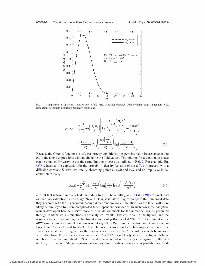
q2�m,s� =2
�j=1
�−1
sin�jm0
�� 2Us� cos�j
��
�2�sin�jm
��
− 2 − 1
�2Us−1� cos�j
��
�2�sin�j�m − 1�
��� . �39�
Because the Green’s functions satisfy reciprocity conditions, it is permissible to interchange m andm0 in the above expressions without changing the field values. The solution for a continuous spacecan be obtained by carrying out the same limiting process as outlined in Ref. 7. For example, Eq.�37� reduces to the expression for the probability density function of the diffusion process with adiffusion constant D with two totally absorbing points at x=0 and x=L and an impulsive initialcondition at x=x0,
p�x,t� =2
Lj=1
�
sin�jx0
L�sin�jx
L�exp�−
2j2Dt
2L2 � , �40�
a result that is found in many texts including Ref. 9. The results given in �34�–�39� are exact, andas such, no validation is necessary. Nevertheless, it is interesting to compare the numerical datathey generate with those generated through direct random walk simulations, as the latter will morelikely be employed for more complicated time-dependent boundaries. In such cases, the analyticalresults developed here will serve more as a validation check for the numerical results generatedthrough random walk simulations. The analytical results �labeled “Ana” in the figures� and theresults obtained by counting the fractional number of paths �labeled “Num” in the figures� in the4RW simulations with initial conditions set at P10=0.5= P20 from the location m0=4 are shown inFigs. 1 and 2 at s=16 and for �=32. For reference, the solution for Schrödinger equation in freespace is also shown in Fig. 2. For the parameters chosen in Fig. 2, the solution with boundarieswill differ from the free-space case only for 0�m�12, as is clearly seen in the figure. A largenumber of realizations �about 108� was needed to arrive at numerically converging results, par-ticularly for the Schrödinger equation whose solution involves difference in probabilities. Both
m
w1
(m∆,
sε)
∆
0 4 8 12 16 20 24 28 320
0.02
0.04
0.06
0.08
0.1
0.12
0.14
0.16
0.18
w1 (Num)w1 (Ana)
P10 = 0.5, P20 = 0.5, P30 = 0, P40 = 0
s = 16, m0 = 4, l = 32
Nr = 107, Nloop = 10
FIG. 1. Comparison of analytical solution for w1�m� ,s��� with that obtained from counting paths in random walksimulations for totally absorbing boundary conditions.
053301-9 Transitional probabilities for the four-state random J. Math. Phys. 50, 053301 �2009�
Downloaded 12 Sep 2010 to 128.119.85.64. Redistribution subject to AIP license or copyright; see http://jmp.aip.org/about/rights_and_permissions

figures reveal that the numerical simulated results closely mimic the analytical formulas derivedhere. The numerical results also underscore the importance of a good numerical random numbergenerator, particularly needed for large s, as the sample size grows exponentially with s. The useof entwined paths described in Ref. 17 is a possible means of getting around this difficulty,although details have only been demonstrated there for the relativistic case of bounded particlespeed.
E. Appropriateness of the 4RW model to wave propagation problems
It might be worthwhile to comment a little on the relationship between the 4RW model andthe continuous parabolic equation for which the former is being targeted in numerical computa-tions. For the parabolic equation encountered in a number of wave propagation problems such asin underwater acoustics, radio wave propagation, and optical wave propagation in fibers, thegoverning equation for the field variable � in a homogeneous medium with time-harmonic exci-tation is of the form
��
�t=
i
2k0
�2�
�x2 , �41�
where the independent variable t denotes the axial spatial coordinate and the variable x denotes thelateral spatial coordinate, k0=2 /� is the wavenumber in the medium, and � is the wavelength ofthe time-harmonic excitation. Equation �41� describes two-dimensional wave propagation in thet-x-plane subject to the approximation that all waves travel within an angle of = �15° about theaxial direction.3 It can be shown that the maximum step size � in the lateral direction is restrictedby ��� / �2 sin max�, where max is the maximum angle of propagation with respect to the t-axis.As is restricted to a value less than 15° for the parabolic approximation to be valid, we may takesin max� tan max�� /�. We then get the approximate relation
� � k0�2. �42�
It may be remarked parenthetically that the inequality �42� translates to the condition that theSchrödinger equation is valid for describing particle motion for nonrelativistic particle speeds withthe normalized speed v /c� tan max�0.27 for max=15°, where c is the speed of light in freespace. In the 4RW model, the relation between the step sizes of the form �=k0�2 is implied andthis is consistent with the inequality �42� If �=� /�2, then this relation implies that �=�. Bothof these values are well within the maximum values permitted by the parabolic equation approxi-mation and it is believed that the 4RW model constitutes a very appropriate discretization schemefor numerically handling the parabolic equation.
m
qk(m�,s�)�
0 4 8 12 16 20 24 28 32-0.4
-0.3
-0.2
-0.1
0
0.1
0.2
0.3
0.4
q1(Num)
q2(Num))
q1(Ana)
q2(Ana)
P10= 0.5, P
20= 0.5, P
30= 0, P
40= 0
s = 16, l = 32, � = 0.707�, � = ��
Nr= 10
7, N
loop= 10, m
0= 4
m
qk(m�,s�)�
0 4 8 12 16 20 24 28 32-0.4
-0.3
-0.2
-0.1
0
0.1
0.2
0.3
0.4
q1(Num)
q1(Ana)
q2(Num)
q2(Ana)
P10= 0.5, P
20= 0.5, P
30= 0; P
40= 0
l = 32, s = 16, m0= 4, � = 0.707�, � = ��
Nr= 10
7, N
loop= 10, T
CPU= 1.8 mins/loop
FIG. 2. �Color online� Comparison of the exact solution of Schrödinger equation with that obtained through counting pathsin random walk simulations.
053301-10 R. Janaswamy J. Math. Phys. 50, 053301 �2009�
Downloaded 12 Sep 2010 to 128.119.85.64. Redistribution subject to AIP license or copyright; see http://jmp.aip.org/about/rights_and_permissions
IV. CONCLUSIONS
Analytical expressions have been provided for the transitional probabilities of a 4RW modelon a lattice constrained in space with dissimilar boundaries and subject to partially reflectingboundary conditions. Special cases of perfectly absorbing boundaries and perfectly reflectingboundaries have been treated. Solution for the transitional probabilities evaluated at time s to thediffusion process is shown to involve sth power of the averaging operator Dx, whereas those of theSchrödinger equation involve Chebyshev polynomials of the second kind of order s and s−1 withargument Dx /�2. These are the general characteristics of diffusion and Schrödinger processes inthe 4RW model irrespective of the boundary conditions. Different boundary conditions will dictatedifferent choices of the eigenfunctions in which the initial probabilities at s=0 are expanded. Theeigenfunctions in the most general case will involve exponential function as well as harmonicfunctions. The exponential function will only exist when the parameters present in the boundaryconditions satisfy certain relationship. While the results presented in this paper should have asignificance of their own for random walk with dissimilar boundaries, it is hoped that they willalso serve as benchmark cases for numerical stochastic methods designed to solve more compli-cated situations. Although it had not been the major focus of the current paper, numerical imple-mentation of the random walk solution necessitates the availability of an effective random numbergenerator to sufficiently populate all portions of the sample space. This is particularly critical forfield evaluated at large times. Extension of these results to higher dimensions and to situationswith a potential field is a topic worthy of further study and will be taken up in the future.
ACKNOWLEDGMENTS
This work was funded in part by the U.S. Army Research Office under ARO Grant No.W911NF-04-1-0228 and by the Center for Advanced Sensor and Communication Antennas, Uni-versity of Massachusetts at Amherst, under the Air Force Research Laboratory Contract No.FA8718-04-C-0057.
1 G. N. Ord and A. S. Deakin, J. Phys. A 30, 819 �1997�.2 G. N. Ord and J. A. Gualtieri, Phys. Rev. Lett. 89, 250403 �2002�.3 F. B. Jensen, W. A. Kuperman, M. B. Porter, and H. Schmidt, Computational Ocean Acoustics �Springer, New York,1994�.
4 J. R. Kuttler and R. Janaswamy, Radio Sci. 37, 5-1 �2002�.5 R. Janaswamy, IEEE Applied Electromagnetics Conference, Kolkata, India, 2007, Vol. 1, Paper No.AEMC.2007.4638046, pp. 1–4; available online at http://ieeexplore.ieee.org/arnumber�4638046&isnumber�4637999&punumber�4629478.
6 B. V. Budaev and D. B. Bogy, Q. J. Mech. Appl. Math. 55, 209 �2002�.7 R. Janaswamy, J. Phys. A: Math. Theor. 41, 155306 �2008�.8 J. C. Strikwerda, Finite Difference Schemes and Partial Differential Equations, 2nd ed. �Society of Industrial andApplied Math, Philadelphia, PA, 2004�.
9 G. H. Weiss, Aspects and Applications of the Random Walk �North-Holland, New York, NY, 1994�.10 F. B. Knight, Essentials of Brownian Motion and Diffusion �American Mathematical Society, New York, NY, 1981�.11 J. Masoliver, J. M. Porra, and G. H. Weiss, Phys. Rev. E 48, 939 �1993�.12 G. N. Ord, Ann. Phys. 250, 51 �1996�.13 G. Barton, Elements of Green’s Functions and Propagation �Oxford University Press, New York, NY, 1989�.14 W. Feller, An Introduction to Probability Theory and Its Applications, 2nd ed. �Wiley, New York, NY, 1970�, Vol. 2.15 E. W. Montroll, J. Math. Phys. 6, 167 �1965�.16 S. A. Martucci, IEEE Trans. Signal Process. 42, 1038 �1994�.17 G. N. Ord, J. A. Gualtieri, and R. B. Mann, Found. Phys. Lett. 19, 471 �2006�.
053301-11 Transitional probabilities for the four-state random J. Math. Phys. 50, 053301 �2009�
Downloaded 12 Sep 2010 to 128.119.85.64. Redistribution subject to AIP license or copyright; see http://jmp.aip.org/about/rights_and_permissions
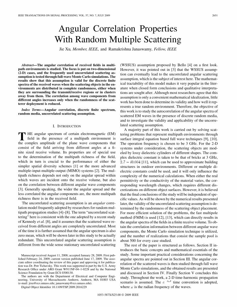
IEEE TRANSACTIONS ON SIGNAL PROCESSING, VOL. 57, NO. 7, JULY 2009 2651
Angular Correlation PropertiesWith Random Multiple Scattering
Jie Xu, Member, IEEE, and Ramakrishna Janaswamy, Fellow, IEEE
Abstract—The angular correlation of received fields in multi-path environments is studied. The focus is put on two-dimensional(2-D) cases, and the frequently used uncorrelated scattering as-sumption is tested through full-wave Monte Carlo simulations. Theresults show that this assumption is valid for the discrete finitespectra of the received waves when the scattering objects in the en-vironments are distributed in complete randomness, either whenthey are surrounding the transmit/receive regions or in clustersaway from them. The correlation among wave components fromdifferent angles increases only when the randomness of the scat-terer deployment is reduced.
Index Terms—Angular correlation, discrete finite spectrum,random media, uncorrelated scattering assumption.
I. INTRODUCTION
T HE angular spectrum of certain electromagnetic (EM)field in the presence of a multipath environment is
the complex amplitude of the plane wave components thatconsist of the field arriving from different angles at a fi-nite sized receive volume. Its properties are of special useto the determination of the multipath richness of the field,which in turn is crucial to the performance of either thesimpler spatial diversity schemes [1] or the more advancedmultiple-input-multiple-output (MIMO) systems [2]. The mul-tipath richness depends not only on the angular spread withinwhich waves are incident onto the receive volume, but alsoon the correlation between different angular wave components[3]. Generally speaking, the wider the angular spread and theless correlated the angular components are, the more multipathrichness there is in the received field.
The uncorrelated scattering assumption is an angular corre-lation model frequently adopted by researchers for random mul-tipath propagation studies [4]–[8]. The term “uncorrelated scat-tering” here is consistent with the one adopted by a recent studyof Kennedy et al. [8], and it assumes that the scattered wave re-ceived from different angles are completely uncorrelated. Mostof the time it is further assumed that the angular spectrum is alsozero mean, which will be shown later in this study to be actuallyredundant. This uncorrelated angular scattering assumption isdifferent from the wide sense stationary uncorrelated scattering
Manuscript received August 11, 2008; accepted January 28, 2009. First pub-lished February 24, 2009; current version published June 17, 2009. The asso-ciate editor coordinating the review of this paper and approving it for publica-tion was Dr. Petr Tichavsky. This work was supported in part by the U.S. ArmyResearch Office under ARO Grant W911NF-04–1-0228 and by the NationalScience Foundation by Grant ECS 0300130.
The authors are with the Department of Electrical and Computer Engi-neering, University of Massachusetts Amherst, Amherst, MA 01003 USA(e-mail: [email protected]; [email protected]).
Digital Object Identifier 10.1109/TSP.2009.2016229
(WSSUS) assumption proposed by Bello [4] on a first look.However, it was pointed out in [3] that the WSSUS assump-tion can eventually lead to the uncorrelated angular scatteringassumption, which is the subject of interest here. The mathemat-ical tractability of this model makes it very popular in the liter-ature when closed form conclusions and qualitative interpreta-tions are sought after. Although most researchers agree that thisassumption is only a convenient mathematical idealization, littlework has been done to determine its validity and how well it rep-resents a true random environment. Therefore, the objective ofthis work is to study the autocorrelation of the angular spectra ofscattered EM waves in the presence of discrete random media,and to investigate the validity and applicability of the uncorre-lated scattering assumption.
A majority part of this work is carried out by solving scat-tering problems that represent multipath environments throughsurface integral equation based full wave techniques [9], [10].The operation frequency is chosen to be 3 GHz. For the 2-Dsystems under consideration, the scattering objects are mod-eled by lossy dielectric cylinders of different shapes. The com-plex dielectric constant is taken to be that of bricks at 3 GHz,
[11], which can be used to approximate buildingstructures in outdoor environments. Different or multiple di-electric constants could be used, and it will only influence thecomplexity of the numerical calculations. When either the realpermittivity or the conductivity of the material varies, the cor-responding wavelength changes, which requires different dis-cretizations on different object surfaces. However, it is believedthat the final conclusions of the study will be independent of spe-cific values. As will be shown by the numerical results presentedlater, the validity of the uncorrelated scattering assumption is de-termined by the randomness of the scattering object placement.For more efficient solution of the problems, the fast multipolemethod (FMM) is used [12], [13], which can directly results inthe angular spectra of the fields in a finite receive volume. To ob-tain the correlation information between different angular wavecomponents, the Monte Carlo simulation technique is utilized,and the number of realizations that consist the sample pool isabout 500 for every case studied.
The rest of the paper is structured as follows. Section II in-troduces the basic concepts and mathematical essentials of thestudy. Some important practical considerations concerning theangular spectra are pointed out in Section III. The angular cor-relation of the scattered waves is then studied through full waveMonte Carlo simulations, and the obtained results are presentedand discussed in Section IV. Finally Section V concludes thisstudy. Throughout the work, a 2-D time-harmonic propagationscenario is assumed. The time convention is adopted,where is the radian frequency of the waves.
1053-587X/$25.00 © 2009 IEEE
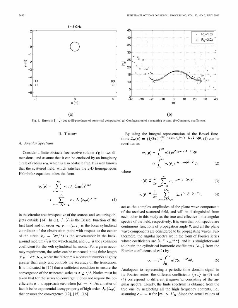
2652 IEEE TRANSACTIONS ON SIGNAL PROCESSING, VOL. 57, NO. 7, JULY 2009
Fig. 1. Errors in �� � due to ill-posedness of numerical computation. (a) Configuration of a scattering system. (b) Computed coefficients.
II. THEORY
A. Angular Spectrum
Consider a finite obstacle free receive volume in two di-mensions, and assume that it can be enclosed by an imaginarycircle of radius , which is also obstacle free. It is well knownthat the scattered field, which satisfies the 2-D homogeneousHelmholtz equation, takes the form
(1)
in the circular area irrespective of the sources and scattering ob-jects outside [14]. In (1), is the Bessel function of thefirst kind and of order , is the local cylindricalcoordinate of the observation point with respect to the centerof the circle, is the wavenumber in the back-ground medium ( is the wavelength), and is the expansioncoefficient for the th cylindrical harmonic. For a given accu-racy requirement, the series can be truncated into a finite length
, where the factor is a constant number slightlygreater than unity and controls the accuracy of the truncation.It is indicated in [15] that a sufficient condition to ensure theconvergence of the truncated series is . Notice must betaken that for the series to converge, it does not require the co-efficients to approach zero when . As a matter offact, it is the exponential decay property of high orderthat ensures the convergence [12], [15], [16].
By using the integral representation of the Bessel func-tions , (1) can berewritten as
(2)
where
(3)
(4)
act as the complex amplitudes of the plane wave componentsof the received scattered field, and will be distinguished fromeach other in this study as the true and effective finite angularspectra of the field, respectively. It is seen that both spectra arecontinuous functions of propagation angle , and all the planewave components are considered to be propagating waves. Fur-thermore, the angular spectra are in the form of Fourier serieswhose coefficients are , and it is straightforwardto obtain the cylindrical harmonic coefficients from theFourier coefficients of by
(5)
Analogous to representing a periodic time domain signal inits Fourier series, the different coefficients in (3) and(4) correspond to different frequencies consisting of the an-gular spectra. Clearly, the finite spectrum is obtained from thetrue one by neglecting all the high frequency contents, i.e.,assuming for . Since the actual values of
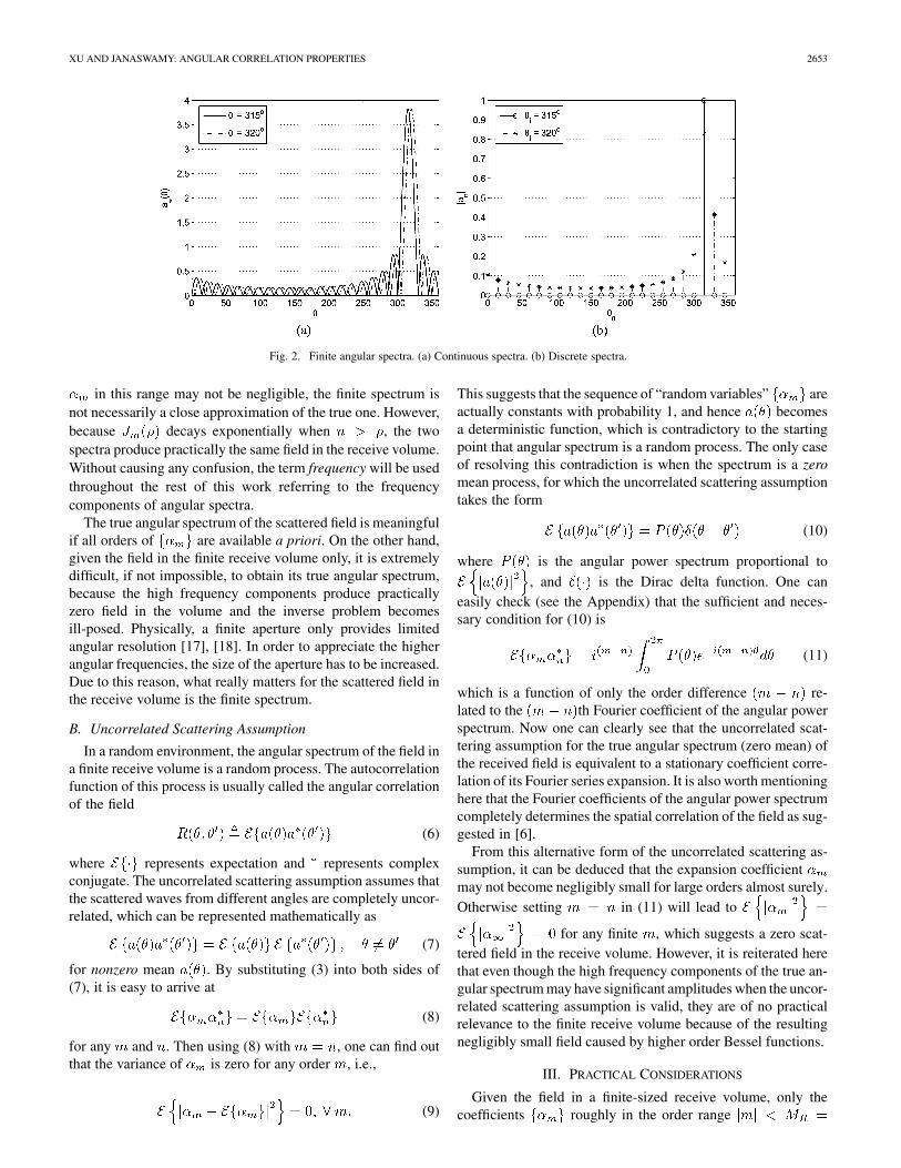
XU AND JANASWAMY: ANGULAR CORRELATION PROPERTIES 2653
Fig. 2. Finite angular spectra. (a) Continuous spectra. (b) Discrete spectra.
in this range may not be negligible, the finite spectrum isnot necessarily a close approximation of the true one. However,because decays exponentially when , the twospectra produce practically the same field in the receive volume.Without causing any confusion, the term frequency will be usedthroughout the rest of this work referring to the frequencycomponents of angular spectra.
The true angular spectrum of the scattered field is meaningfulif all orders of are available a priori. On the other hand,given the field in the finite receive volume only, it is extremelydifficult, if not impossible, to obtain its true angular spectrum,because the high frequency components produce practicallyzero field in the volume and the inverse problem becomesill-posed. Physically, a finite aperture only provides limitedangular resolution [17], [18]. In order to appreciate the higherangular frequencies, the size of the aperture has to be increased.Due to this reason, what really matters for the scattered field inthe receive volume is the finite spectrum.
B. Uncorrelated Scattering Assumption
In a random environment, the angular spectrum of the field ina finite receive volume is a random process. The autocorrelationfunction of this process is usually called the angular correlationof the field
(6)
where represents expectation and represents complexconjugate. The uncorrelated scattering assumption assumes thatthe scattered waves from different angles are completely uncor-related, which can be represented mathematically as
(7)
for nonzero mean . By substituting (3) into both sides of(7), it is easy to arrive at
(8)
for any and . Then using (8) with , one can find outthat the variance of is zero for any order , i.e.,
(9)
This suggests that the sequence of “random variables” areactually constants with probability 1, and hence becomesa deterministic function, which is contradictory to the startingpoint that angular spectrum is a random process. The only caseof resolving this contradiction is when the spectrum is a zeromean process, for which the uncorrelated scattering assumptiontakes the form
(10)
where is the angular power spectrum proportional to
, and is the Dirac delta function. One caneasily check (see the Appendix) that the sufficient and neces-sary condition for (10) is
(11)
which is a function of only the order difference re-lated to the th Fourier coefficient of the angular powerspectrum. Now one can clearly see that the uncorrelated scat-tering assumption for the true angular spectrum (zero mean) ofthe received field is equivalent to a stationary coefficient corre-lation of its Fourier series expansion. It is also worth mentioninghere that the Fourier coefficients of the angular power spectrumcompletely determines the spatial correlation of the field as sug-gested in [6].
From this alternative form of the uncorrelated scattering as-sumption, it can be deduced that the expansion coefficientmay not become negligibly small for large orders almost surely.Otherwise setting in (11) will lead to
for any finite , which suggests a zero scat-tered field in the receive volume. However, it is reiterated herethat even though the high frequency components of the true an-gular spectrum may have significant amplitudes when the uncor-related scattering assumption is valid, they are of no practicalrelevance to the finite receive volume because of the resultingnegligibly small field caused by higher order Bessel functions.
III. PRACTICAL CONSIDERATIONS
Given the field in a finite-sized receive volume, only thecoefficients roughly in the order range
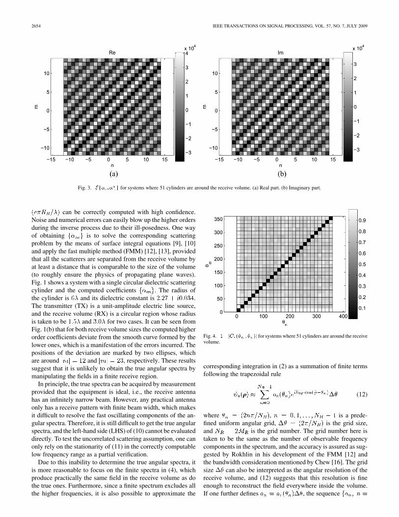
2654 IEEE TRANSACTIONS ON SIGNAL PROCESSING, VOL. 57, NO. 7, JULY 2009
Fig. 3. ��� � � for systems where 51 cylinders are around the receive volume. (a) Real part. (b) Imaginary part.
can be correctly computed with high confidence.Noise and numerical errors can easily blow up the higher ordersduring the inverse process due to their ill-posedness. One wayof obtaining is to solve the corresponding scatteringproblem by the means of surface integral equations [9], [10]and apply the fast multiple method (FMM) [12], [13], providedthat all the scatterers are separated from the receive volume byat least a distance that is comparable to the size of the volume(to roughly ensure the physics of propagating plane waves).Fig. 1 shows a system with a single circular dielectric scatteringcylinder and the computed coefficients . The radius ofthe cylinder is and its dielectric constant is .The transmitter (TX) is a unit-amplitude electric line source,and the receive volume (RX) is a circular region whose radiusis taken to be and for two cases. It can be seen fromFig. 1(b) that for both receive volume sizes the computed higherorder coefficients deviate from the smooth curve formed by thelower ones, which is a manifestation of the errors incurred. Thepositions of the deviation are marked by two ellipses, whichare around and , respectively. These resultssuggest that it is unlikely to obtain the true angular spectra bymanipulating the fields in a finite receive region.
In principle, the true spectra can be acquired by measurementprovided that the equipment is ideal, i.e., the receive antennahas an infinitely narrow beam. However, any practical antennaonly has a receive pattern with finite beam width, which makesit difficult to resolve the fast oscillating components of the an-gular spectra. Therefore, it is still difficult to get the true angularspectra, and the left-hand side (LHS) of (10) cannot be evaluateddirectly. To test the uncorrelated scattering assumption, one canonly rely on the stationarity of (11) in the correctly computablelow frequency range as a partial verification.
Due to this inability to determine the true angular spectra, itis more reasonable to focus on the finite spectra in (4), whichproduce practically the same field in the receive volume as dothe true ones. Furthermore, since a finite spectrum excludes allthe higher frequencies, it is also possible to approximate the
Fig. 4. ���� �� � � �� for systems where 51 cylinders are around the receivevolume.
corresponding integration in (2) as a summation of finite termsfollowing the trapezoidal rule
(12)
where , is a prede-fined uniform angular grid, is the grid size,and is the grid number. The grid number here istaken to be the same as the number of observable frequencycomponents in the spectrum, and the accuracy is assured as sug-gested by Rokhlin in his development of the FMM [12] andthe bandwidth consideration mentioned by Chew [16]. The gridsize can also be interpreted as the angular resolution of thereceive volume, and (12) suggests that this resolution is fineenough to reconstruct the field everywhere inside the volume.If one further defines , the sequence

XU AND JANASWAMY: ANGULAR CORRELATION PROPERTIES 2655
Fig. 5. System with four groups of three cylinders around the receive volume. (a) ���� � ��. (b) �� �� �� � � ��.
constitutes a discrete finite spectrum of the re-ceived scattered field.
The finite spectrum does not satisfy the uncorrelated scat-tering assumption because it is easy to check that the correla-tion between its Fourier coefficients of various orders is not sta-tistically stationary. Even so, it is still possible that two of itsangular components that are separated far enough are uncorre-lated or only weakly correlated, which mathematically means
(13)
with . Furthermore, due to the limited angularresolution associated with the finite receive volume, it is un-necessary to seek for correlation between angles separated lessthan the resolution size . Therefore, it would be interestingto test if (13) is true for . In the numerical results pre-sented in Section IV, the angular correlation will only be evalu-ated among the discrete wave angles . Moreover, for betterillustration of the results, the normalized autocorrelation coeffi-cient is considered
(14)
Another issue worth mentioning is the relation between thetrue and finite angular spectra. Compared to the true spectrum,even though the finite one ignores all the high frequency compo-nents for , which might actually have significantamplitude, it is still possible that the two resemble each otherquite well (see the example that follows). When the discrete fi-nite spectra are considered, the errors come not only from thefrequency domain truncation, but also possibly from angle mis-matching, which is also demonstrated by the following example.
When a single plane wave is incident upon a circular re-ceive volume centered at the origin, the true angular spectrumis clearly nonzero for only one angle, i.e., ,where is the incident angle. The corresponding coefficientsare , which are of unit magnitude up to infi-nite order. Suppose the radius of the receive volume is , the
finite spectrum includes low frequency components.Fig. 2 shows the continuous and discrete finite angular spectra
and with incident angle and . Theripples in the continuous finite spectra of Fig. 2(a) are obviouslycaused by ignoring the high frequency components. However,the strong peaks in the figure correctly identify the incident an-gles. For the discrete finite spectra in Fig. 2(b), when ,it is correctly indicated that there is only one angular compo-nent. However, when , all the other components arealso present. This is because is one of the pre-definedangles while is not. The mismatching betweenthe incident angle and the uniform grid requires all angular com-ponents to appear as a compensation.
IV. SIMULATION RESULTS
This section studies a number of different scenarios and thevalidity of the uncorrelated scattering assumption is tested. Inthe first system studied, a line source transmitter and a circularreceive volume of radius are separated by . Dielectricscattering cylinders of different shapes are randomly distributedin a circular ring around the receive volume in a nearly uniformway, with the only requirement being that the scatterers do notoverlap with each other. The inner radius of the ring is andthe outer radius is . The shapes of the cylinder can be cir-cular, elliptical, or square, but they all have the same perimeter
. Fig. 3 shows the grayscale plots of the real and imaginaryparts of the correlation when the number of cylindersis 51 (corresponding to a scatterer area density around 11.5%).It can be seen that is only a function of the differ-ence between the two indices and . This stationarity sug-gests that it is likely that the true angular spectra satisfy the un-correlated scattering assumption. To accentuate high correlationwith dark grayscale, Fig. 4 shows the amplitude of the simulatedcomplementary angular correlation of the discrete finite spectra,i.e., . For the complementary correlation coef-ficient, values close to zero indicate high correlation. The wavesfrom two distinct discrete angles are seen to be almost uncorre-lated, suggesting that (13) is valid. The few weakly correlated
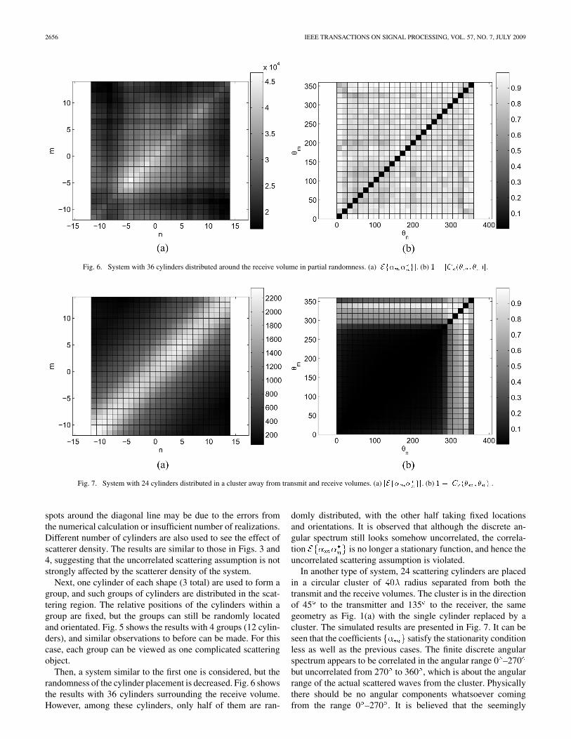
2656 IEEE TRANSACTIONS ON SIGNAL PROCESSING, VOL. 57, NO. 7, JULY 2009
Fig. 6. System with 36 cylinders distributed around the receive volume in partial randomness. (a) ���� � ��. (b) �� �� �� � � ��.
Fig. 7. System with 24 cylinders distributed in a cluster away from transmit and receive volumes. (a) ���� � ��. (b) �� �� �� � � ��.
spots around the diagonal line may be due to the errors fromthe numerical calculation or insufficient number of realizations.Different number of cylinders are also used to see the effect ofscatterer density. The results are similar to those in Figs. 3 and4, suggesting that the uncorrelated scattering assumption is notstrongly affected by the scatterer density of the system.
Next, one cylinder of each shape (3 total) are used to form agroup, and such groups of cylinders are distributed in the scat-tering region. The relative positions of the cylinders within agroup are fixed, but the groups can still be randomly locatedand orientated. Fig. 5 shows the results with 4 groups (12 cylin-ders), and similar observations to before can be made. For thiscase, each group can be viewed as one complicated scatteringobject.
Then, a system similar to the first one is considered, but therandomness of the cylinder placement is decreased. Fig. 6 showsthe results with 36 cylinders surrounding the receive volume.However, among these cylinders, only half of them are ran-
domly distributed, with the other half taking fixed locationsand orientations. It is observed that although the discrete an-gular spectrum still looks somehow uncorrelated, the correla-tion is no longer a stationary function, and hence theuncorrelated scattering assumption is violated.
In another type of system, 24 scattering cylinders are placedin a circular cluster of radius separated from both thetransmit and the receive volumes. The cluster is in the directionof 45 to the transmitter and 135 to the receiver, the samegeometry as Fig. 1(a) with the single cylinder replaced by acluster. The simulated results are presented in Fig. 7. It can beseen that the coefficients satisfy the stationarity conditionless as well as the previous cases. The finite discrete angularspectrum appears to be correlated in the angular range 0 –270but uncorrelated from 270 to 360 , which is about the angularrange of the actual scattered waves from the cluster. Physicallythere should be no angular components whatsoever comingfrom the range 0 –270 . It is believed that the seemingly
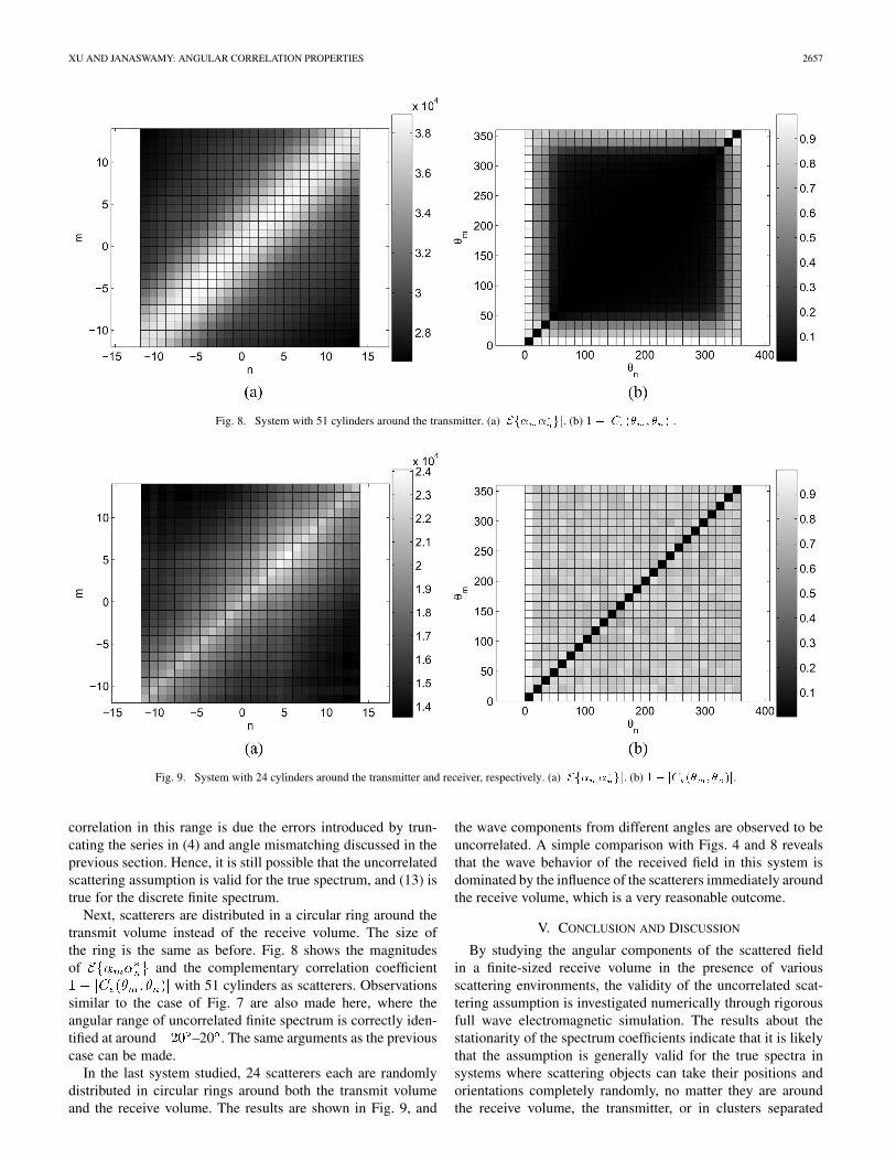
XU AND JANASWAMY: ANGULAR CORRELATION PROPERTIES 2657
Fig. 8. System with 51 cylinders around the transmitter. (a) ���� � ��. (b) �� �� �� � � ��.
Fig. 9. System with 24 cylinders around the transmitter and receiver, respectively. (a) ���� � ��. (b) �� �� �� � � ��.
correlation in this range is due the errors introduced by trun-cating the series in (4) and angle mismatching discussed in theprevious section. Hence, it is still possible that the uncorrelatedscattering assumption is valid for the true spectrum, and (13) istrue for the discrete finite spectrum.
Next, scatterers are distributed in a circular ring around thetransmit volume instead of the receive volume. The size ofthe ring is the same as before. Fig. 8 shows the magnitudesof and the complementary correlation coefficient
with 51 cylinders as scatterers. Observationssimilar to the case of Fig. 7 are also made here, where theangular range of uncorrelated finite spectrum is correctly iden-tified at around –20 . The same arguments as the previouscase can be made.
In the last system studied, 24 scatterers each are randomlydistributed in circular rings around both the transmit volumeand the receive volume. The results are shown in Fig. 9, and
the wave components from different angles are observed to beuncorrelated. A simple comparison with Figs. 4 and 8 revealsthat the wave behavior of the received field in this system isdominated by the influence of the scatterers immediately aroundthe receive volume, which is a very reasonable outcome.
V. CONCLUSION AND DISCUSSION
By studying the angular components of the scattered fieldin a finite-sized receive volume in the presence of variousscattering environments, the validity of the uncorrelated scat-tering assumption is investigated numerically through rigorousfull wave electromagnetic simulation. The results about thestationarity of the spectrum coefficients indicate that it is likelythat the assumption is generally valid for the true spectra insystems where scattering objects can take their positions andorientations completely randomly, no matter they are aroundthe receive volume, the transmitter, or in clusters separated

2658 IEEE TRANSACTIONS ON SIGNAL PROCESSING, VOL. 57, NO. 7, JULY 2009
from them. In the meanwhile, the results of the correlation co-efficients among the discrete plane wave components directlysuggest that the discrete finite spectra are also likely to be un-correlated when the scattering object placement is completelyrandom. However, as soon as the randomness of the scattererplacement is decreased, the assumption is observed to breakdown in the sense that the correlation of the spectrum expansioncoefficients is no longer stationary. Intuitively, there is a directcause-effect relationship between the randomness of the scat-terer deployment and the validity of the uncorrelated scatteringassumption. In outdoor environments where a large number ofobjects can move around freely, this assumption might be agood model to describe the multipath wave propagation.
The case when the receiver is moving with constant velocityis of special interest when properties such as space-time crosscorrelation and space-frequency cross correlation are desired[19]. For such cases, the field as a function of the receiver loca-tion, which in turn is a function of time , can be obtained from(2) as , where
is the initial location of the receiver, is themaximum Doppler frequency shift, and is the direction anglein which the receiver moves at velocity . Similar analysis canbe carried out and the same conclusion about the angular cor-relation of the wave spectrum can be reached, provided that thereceiver does not move out of the receive volume. Outside thevolume, the starting (1) may not be valid.
Furthermore, even though the study presented here is onlyfor the received field, the transmit side can be included simplyby considering reciprocity of the systems, and the uncorrelatedscattering assumption can be easily extended to the double-an-gular domain. Specifically, the field in the receive volume asthe response to some source in the transmit volume can be ex-pressed as a combination of plane waves arriving at the receivevolume in different angles of arrival (AOA) due to a series ofplane waves leaving the transmit volume in different angles ofdeparture (AOD). When the scattering objects are distributed incomplete randomness, the coefficients of all these plane wavecomponents are uncorrelated pairwise. This extended assump-tion has been successfully applied in a recent work of the au-thors to develop a statistical propagation model between finitetransmit and receive volumes [20].
APPENDIX
ALTERNATIVE FORM OF UNCORRELATED
SCATTERING ASSUMPTION
It is proved here that the sufficient and necessary conditionfor the uncorrelated scattering assumption in (10) is (11). Thenecessity is shown first.
Necessity: By substituting (3) in the LHS of (10) and usingthe Fourier expansion of the Dirac delta function on the right-hand side (RHS), (10) becomes
(15)
Matching the Fourier coefficients on both sides and some simplemanipulations will lead to
(16)
which represents the power angular spectrum in a Fourier series.Using the standard way to calculate the Fourier coefficients, onearrives at the final form of (11)
(17)
This completes the proof of necessity.Sufficiency: The LHS of (10) can be represented as
(18)
Substituting (17) into (18), one obtains
(19)
which is exactly (10). This completes the proof of sufficiency.
REFERENCES
[1] W. C. Jakes, Microwave Mobile Communications. Piscataway, NJ:IEEE, 1994.
[2] G. J. Foschini and M. J. Gans, “On limits of wireless communicationsin a fading enviroment when using multiple antennas,” IEEE J. Sel.Areas Commun., vol. 6, pp. 331–335, Mar. 1998.
[3] T. Betlehem and T. D. Abhayapala, “Spatial correlation for correlatedscatterers,” in Proc. IEEE Int. Conf. Acoust., Speech, Signal Process.(ICASSP), Toulouse, France, May 2006.
[4] P. A. Bello, “Characterization of randomly time-variant linear chan-nels,” IEEE Trans. Commun. Syst., vol. CS-11, pp. 360–393, Dec. 1963.
[5] J. D. Parsons, The Mobile Radio Propagation Channel. London,U.K.: Pentech, 1992.
[6] P. D. Teal, T. D. Abhayapala, and R. A. Kennedy, “Spatial correlationfor general distributions of scatterers,” IEEE Signal Process. Lett., vol.9, pp. 305–308, Oct. 2002.
[7] A. S. Y. Poon, R. W. Brodersen, and D. N. C. Tse, “Degrees of freedomin multiple-antenna channels: A signal space approach,” IEEE Trans.Inf. Theory, vol. 51, pp. 523–536, Feb. 2005.
[8] R. A. Kennedy, P. S. Sadeghi, T. D. Abhayapala, and H. M. Jones,“Instrinsic limits of dimensionality and richness in random multipathfields,” IEEE Trans. Signal Process., vol. 55, pp. 2542–2556, Jun. 2007.
[9] D. Colton and R. Kress, Integral Equation Methods in ScatteringTheory. New York: Wiley, 1983.
[10] F. Seydou, R. Duraiswami, and T. Seppänen, “A boundary elementmethod for electromagnetic scattering by multiple cylinders,” in Proc.IEEE AP-S Int. Symp. Dig., Columbus, OH, Jun. 2003, vol. 3, pp.516–519.
[11] R. V. Hippel, Dielectric Materials and Applications. Cambridge,MA: Mass. Inst. Technol. Press, 1954.
[12] V. Rokhlin, “Rapid solution of integral equations of scattering theoryin two dimensions,” J. Comput. Phys., vol. 86, pp. 414–439, Feb. 1990.

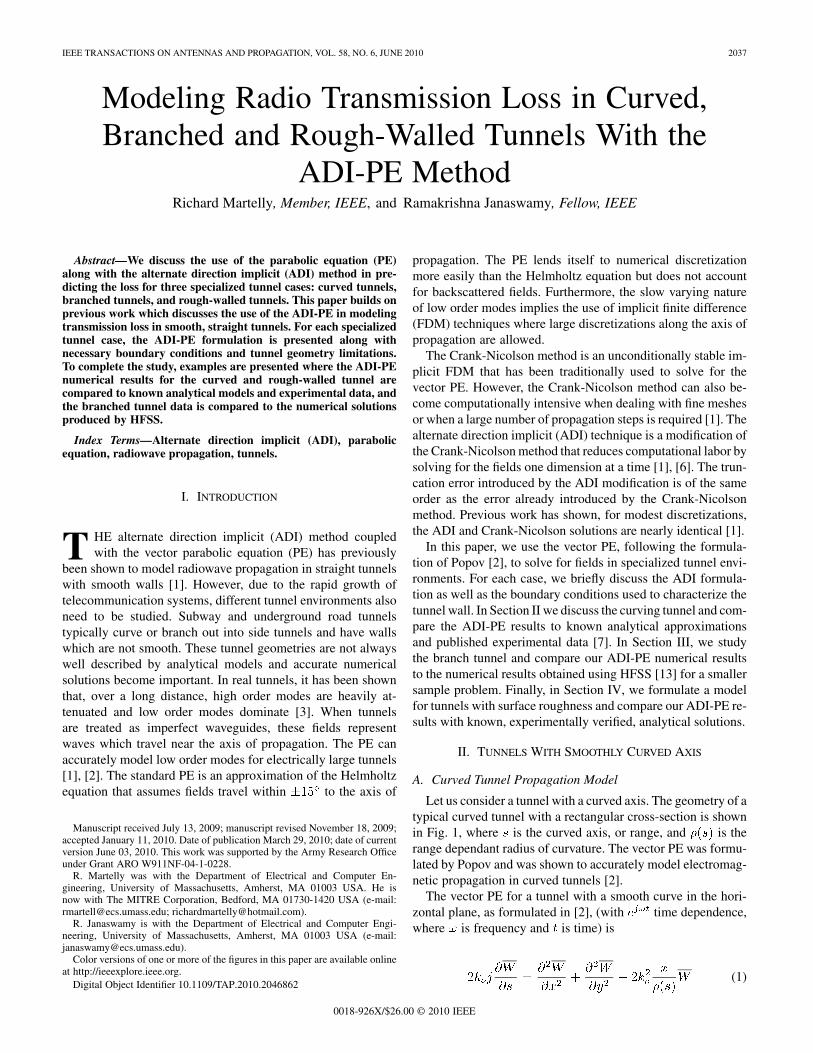
IEEE TRANSACTIONS ON ANTENNAS AND PROPAGATION, VOL. 58, NO. 6, JUNE 2010 2037
Modeling Radio Transmission Loss in Curved,Branched and Rough-Walled Tunnels With the
ADI-PE MethodRichard Martelly, Member, IEEE, and Ramakrishna Janaswamy, Fellow, IEEE
Abstract—We discuss the use of the parabolic equation (PE)along with the alternate direction implicit (ADI) method in pre-dicting the loss for three specialized tunnel cases: curved tunnels,branched tunnels, and rough-walled tunnels. This paper builds onprevious work which discusses the use of the ADI-PE in modelingtransmission loss in smooth, straight tunnels. For each specializedtunnel case, the ADI-PE formulation is presented along withnecessary boundary conditions and tunnel geometry limitations.To complete the study, examples are presented where the ADI-PEnumerical results for the curved and rough-walled tunnel arecompared to known analytical models and experimental data, andthe branched tunnel data is compared to the numerical solutionsproduced by HFSS.
Index Terms—Alternate direction implicit (ADI), parabolicequation, radiowave propagation, tunnels.
I. INTRODUCTION
T HE alternate direction implicit (ADI) method coupledwith the vector parabolic equation (PE) has previously
been shown to model radiowave propagation in straight tunnelswith smooth walls [1]. However, due to the rapid growth oftelecommunication systems, different tunnel environments alsoneed to be studied. Subway and underground road tunnelstypically curve or branch out into side tunnels and have wallswhich are not smooth. These tunnel geometries are not alwayswell described by analytical models and accurate numericalsolutions become important. In real tunnels, it has been shownthat, over a long distance, high order modes are heavily at-tenuated and low order modes dominate [3]. When tunnelsare treated as imperfect waveguides, these fields representwaves which travel near the axis of propagation. The PE canaccurately model low order modes for electrically large tunnels[1], [2]. The standard PE is an approximation of the Helmholtzequation that assumes fields travel within to the axis of
Manuscript received July 13, 2009; manuscript revised November 18, 2009;accepted January 11, 2010. Date of publication March 29, 2010; date of currentversion June 03, 2010. This work was supported by the Army Research Officeunder Grant ARO W911NF-04-1-0228.
R. Martelly was with the Department of Electrical and Computer En-gineering, University of Massachusetts, Amherst, MA 01003 USA. He isnow with The MITRE Corporation, Bedford, MA 01730-1420 USA (e-mail:[email protected]; [email protected]).
R. Janaswamy is with the Department of Electrical and Computer Engi-neering, University of Massachusetts, Amherst, MA 01003 USA (e-mail:[email protected]).
Color versions of one or more of the figures in this paper are available onlineat http://ieeexplore.ieee.org.
Digital Object Identifier 10.1109/TAP.2010.2046862
propagation. The PE lends itself to numerical discretizationmore easily than the Helmholtz equation but does not accountfor backscattered fields. Furthermore, the slow varying natureof low order modes implies the use of implicit finite difference(FDM) techniques where large discretizations along the axis ofpropagation are allowed.
The Crank-Nicolson method is an unconditionally stable im-plicit FDM that has been traditionally used to solve for thevector PE. However, the Crank-Nicolson method can also be-come computationally intensive when dealing with fine meshesor when a large number of propagation steps is required [1]. Thealternate direction implicit (ADI) technique is a modification ofthe Crank-Nicolson method that reduces computational labor bysolving for the fields one dimension at a time [1], [6]. The trun-cation error introduced by the ADI modification is of the sameorder as the error already introduced by the Crank-Nicolsonmethod. Previous work has shown, for modest discretizations,the ADI and Crank-Nicolson solutions are nearly identical [1].
In this paper, we use the vector PE, following the formula-tion of Popov [2], to solve for fields in specialized tunnel envi-ronments. For each case, we briefly discuss the ADI formula-tion as well as the boundary conditions used to characterize thetunnel wall. In Section II we discuss the curving tunnel and com-pare the ADI-PE results to known analytical approximationsand published experimental data [7]. In Section III, we studythe branch tunnel and compare our ADI-PE numerical resultsto the numerical results obtained using HFSS [13] for a smallersample problem. Finally, in Section IV, we formulate a modelfor tunnels with surface roughness and compare our ADI-PE re-sults with known, experimentally verified, analytical solutions.
II. TUNNELS WITH SMOOTHLY CURVED AXIS
A. Curved Tunnel Propagation Model
Let us consider a tunnel with a curved axis. The geometry of atypical curved tunnel with a rectangular cross-section is shownin Fig. 1, where is the curved axis, or range, and is therange dependant radius of curvature. The vector PE was formu-lated by Popov and was shown to accurately model electromag-netic propagation in curved tunnels [2].
The vector PE for a tunnel with a smooth curve in the hori-zontal plane, as formulated in [2], (with time dependence,where is frequency and is time) is
(1)
0018-926X/$26.00 © 2010 IEEE
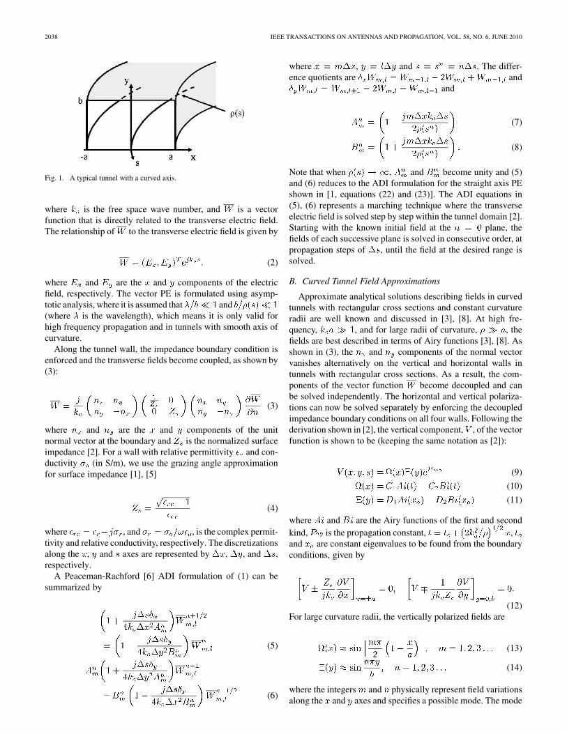
2038 IEEE TRANSACTIONS ON ANTENNAS AND PROPAGATION, VOL. 58, NO. 6, JUNE 2010
Fig. 1. A typical tunnel with a curved axis.
where is the free space wave number, and is a vectorfunction that is directly related to the transverse electric field.The relationship of to the transverse electric field is given by
(2)
where and are the and components of the electricfield, respectively. The vector PE is formulated using asymp-totic analysis, where it is assumed that and(where is the wavelength), which means it is only valid forhigh frequency propagation and in tunnels with smooth axis ofcurvature.
Along the tunnel wall, the impedance boundary condition isenforced and the transverse fields become coupled, as shown by(3):
(3)
where and are the and components of the unitnormal vector at the boundary and is the normalized surfaceimpedance [2]. For a wall with relative permittivity and con-ductivity (in S/m), we use the grazing angle approximationfor surface impedance [1], [5]
(4)
where , and , is the complex permit-tivity and relative conductivity, respectively. The discretizationsalong the , and axes are represented by , , and ,respectively.
A Peaceman-Rachford [6] ADI formulation of (1) can besummarized by
(5)
(6)
where , and . The differ-ence quotients are and
and
(7)
(8)
Note that when , and become unity and (5)and (6) reduces to the ADI formulation for the straight axis PEshown in [1, equations (22) and (23)]. The ADI equations in(5), (6) represents a marching technique where the transverseelectric field is solved step by step within the tunnel domain [2].Starting with the known initial field at the plane, thefields of each successive plane is solved in consecutive order, atpropagation steps of , until the field at the desired range issolved.
B. Curved Tunnel Field Approximations
Approximate analytical solutions describing fields in curvedtunnels with rectangular cross sections and constant curvatureradii are well known and discussed in [3], [8]. At high fre-quency, , and for large radii of curvature, , thefields are best described in terms of Airy functions [3], [8]. Asshown in (3), the and components of the normal vectorvanishes alternatively on the vertical and horizontal walls intunnels with rectangular cross sections. As a result, the com-ponents of the vector function become decoupled and canbe solved independently. The horizontal and vertical polariza-tions can now be solved separately by enforcing the decoupledimpedance boundary conditions on all four walls. Following thederivation shown in [2], the vertical component, , of the vectorfunction is shown to be (keeping the same notation as [2]):
(9)
(10)
(11)
where and are the Airy functions of the first and secondkind, is the propagation constant, ,and are constant eigenvalues to be found from the boundaryconditions, given by
(12)For large curvature radii, the vertically polarized fields are
(13)
(14)
where the integers and physically represent field variationsalong the and axes and specifies a possible mode. The mode

MARTELLY AND JANASWAMY: MODELING RADIO TRANSMISSION LOSS IN CURVED, BRANCHED AND ROUGH-WALLED TUNNELS 2039
TABLE IANALYTICAL AND NUMERICAL MAFS FOR THE CURVED TUNNEL WITH
RECTANGULAR CROSS SECTION FOR 950 MHZ
attenuation per unit length can be found from the complex ex-ponent, , to be [2]
(15)
where
(16)and . The part of (15) de-scribes small radii of curvature and the part de-scribes large radii of curvature (or almost straight tunnels). Mah-moud and Wait [9] numerically calculated the attenuation fac-tors for curved waveguides using more precise transcendentalequations. As shown in [2, Fig. 3], the aysmptotic equation (15)is in very good agreement with Mahmoud and Wait’s numericalsolutions. We will use the aysmptotic equation to validate thenumerical simulations of the ADI-PE.
C. Comparison of the ADI-PE to Analytical Solutions
In this sub-section, we validate the ADI-PE with numericalexamples. We consider a rectangular tunnel with dimensionsof 8 m 4 m and walls with relative dielectric constant,
, and conductivity, . We used the dominantmode of the vertically polarized field, as shown
by (13) and (14), as our initial field. The discretizations usedfor the 950 MHz case were , and
; and the discretizations used for the 1.8 GHzsimulations were , and .
The mode attenuations per unit length, or mode attenuationfactors (MAFs), from (15) and the ADI-PE simulations are tab-ulated in Tables I and II for different curvature radii.
As shown in Tables I and II, the numerical MAFs closelyfollow the aysmptotic solutions over the range of curvature radii.Furthermore, as the curvature radii decreases, the number ofreflections from the walls along the curved path increases andso does the loss. The percent error, defined by
(17)
TABLE IIANALYTICAL AND NUMERICAL MAFS FOR THE CURVED TUNNEL WITH
RECTANGULAR CROSS SECTION FOR 1.8 GHZ
Fig. 2. Percent error of the MAFs of the curved waveguide for 950 MHz (dot,solid) and 1.8 GHz (circle, solid) for �� � ���� �. The percent error ofthe MAFs for 950 MHz (dot,dashed) and 1.8 GHz (circle, dashed) for �� �
����� �. The vertical lines show the region where � � �� for 950 MHz(solid) and 1.8 GHz (dashed).
is shown in Fig. 2 as a function of , (where is the lengthof the diagonal of the rectangular cross section) for 950 MHz(dot, solid) and 1.8 GHz (circle, solid). The figure also shows theresults for smaller discretizations ( ) with dashedcurves to show that the solutions are convergent. The verticallines in Fig. 2 show the region where for the 950 MHz(solid) and 1.8 GHz (dashed) cases, respectively. The parameter,
, was selected from [2] because it is a wavelength depen-dent term that must be much less than unity to ensure accurateresults. Furthermore, , is the Fresnel number and is oneof the parameters which govern the diffraction processes in thewaveguide [2]. As Fig. 2 shows, there is less than 5% error inMAFs over the entire range of considered; even when thereare sharp bends and the condition, , is not satisfied.Finally, one of the important characteristics of the curved tunnelis the accumulation of the field near the concave wall at(the whispering gallery mode). Fig. 3(a) shows the dominant
field as defined by (13) and (14) across the initialplane at 1.8 GHz. The whispering gallery mode feature can beseen in Fig. 3(b), where the field generated by the ADI-PE, ata range of 2000 m for , has an accumulation alongthe wall.
D. Comparison of the ADI-PE to Ray Tracing Simulations
In this section, we compare the ADI-PE simulations to the raytracing simulations shown in Wang et al. for a curved waveguide[7]. The geometry of the waveguide (top view) is shown in Fig. 4and is comprised of two straight sections and a curved section.
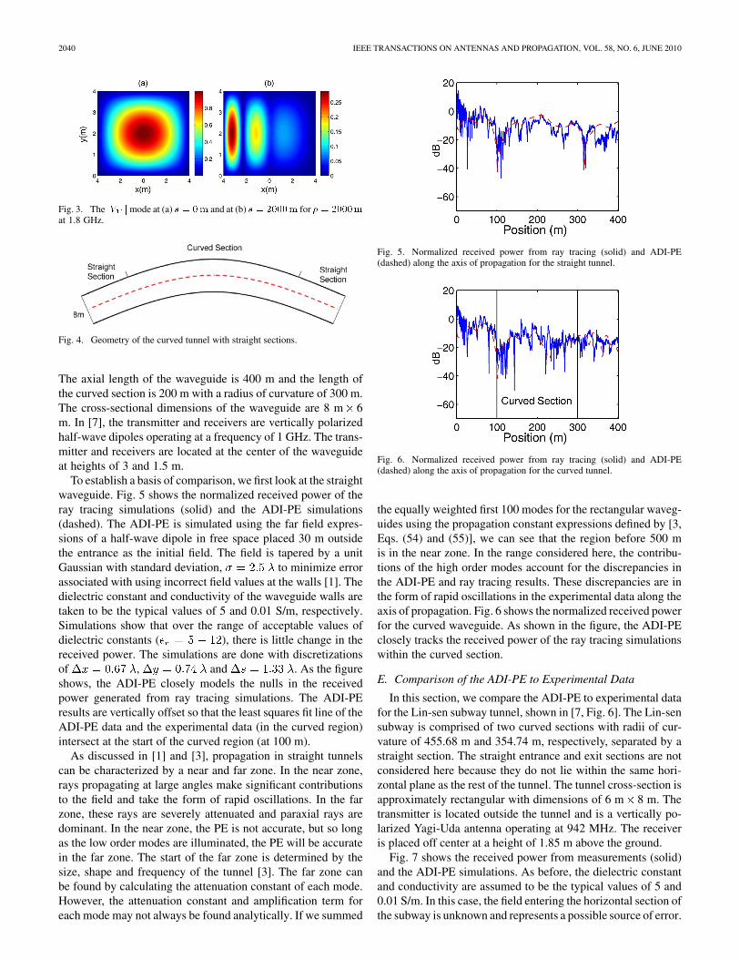
2040 IEEE TRANSACTIONS ON ANTENNAS AND PROPAGATION, VOL. 58, NO. 6, JUNE 2010
Fig. 3. The �� � mode at (a) � � �� and at (b) � � ����� for � � �����
at 1.8 GHz.
Fig. 4. Geometry of the curved tunnel with straight sections.
The axial length of the waveguide is 400 m and the length ofthe curved section is 200 m with a radius of curvature of 300 m.The cross-sectional dimensions of the waveguide are 8 m 6m. In [7], the transmitter and receivers are vertically polarizedhalf-wave dipoles operating at a frequency of 1 GHz. The trans-mitter and receivers are located at the center of the waveguideat heights of 3 and 1.5 m.
To establish a basis of comparison, we first look at the straightwaveguide. Fig. 5 shows the normalized received power of theray tracing simulations (solid) and the ADI-PE simulations(dashed). The ADI-PE is simulated using the far field expres-sions of a half-wave dipole in free space placed 30 m outsidethe entrance as the initial field. The field is tapered by a unitGaussian with standard deviation, to minimize errorassociated with using incorrect field values at the walls [1]. Thedielectric constant and conductivity of the waveguide walls aretaken to be the typical values of 5 and 0.01 S/m, respectively.Simulations show that over the range of acceptable values ofdielectric constants ( ), there is little change in thereceived power. The simulations are done with discretizationsof , and . As the figureshows, the ADI-PE closely models the nulls in the receivedpower generated from ray tracing simulations. The ADI-PEresults are vertically offset so that the least squares fit line of theADI-PE data and the experimental data (in the curved region)intersect at the start of the curved region (at 100 m).
As discussed in [1] and [3], propagation in straight tunnelscan be characterized by a near and far zone. In the near zone,rays propagating at large angles make significant contributionsto the field and take the form of rapid oscillations. In the farzone, these rays are severely attenuated and paraxial rays aredominant. In the near zone, the PE is not accurate, but so longas the low order modes are illuminated, the PE will be accuratein the far zone. The start of the far zone is determined by thesize, shape and frequency of the tunnel [3]. The far zone canbe found by calculating the attenuation constant of each mode.However, the attenuation constant and amplification term foreach mode may not always be found analytically. If we summed
Fig. 5. Normalized received power from ray tracing (solid) and ADI-PE(dashed) along the axis of propagation for the straight tunnel.
Fig. 6. Normalized received power from ray tracing (solid) and ADI-PE(dashed) along the axis of propagation for the curved tunnel.
the equally weighted first 100 modes for the rectangular waveg-uides using the propagation constant expressions defined by [3,Eqs. (54) and (55)], we can see that the region before 500 mis in the near zone. In the range considered here, the contribu-tions of the high order modes account for the discrepancies inthe ADI-PE and ray tracing results. These discrepancies are inthe form of rapid oscillations in the experimental data along theaxis of propagation. Fig. 6 shows the normalized received powerfor the curved waveguide. As shown in the figure, the ADI-PEclosely tracks the received power of the ray tracing simulationswithin the curved section.
E. Comparison of the ADI-PE to Experimental Data
In this section, we compare the ADI-PE to experimental datafor the Lin-sen subway tunnel, shown in [7, Fig. 6]. The Lin-sensubway is comprised of two curved sections with radii of cur-vature of 455.68 m and 354.74 m, respectively, separated by astraight section. The straight entrance and exit sections are notconsidered here because they do not lie within the same hori-zontal plane as the rest of the tunnel. The tunnel cross-section isapproximately rectangular with dimensions of 6 m 8 m. Thetransmitter is located outside the tunnel and is a vertically po-larized Yagi-Uda antenna operating at 942 MHz. The receiveris placed off center at a height of 1.85 m above the ground.
Fig. 7 shows the received power from measurements (solid)and the ADI-PE simulations. As before, the dielectric constantand conductivity are assumed to be the typical values of 5 and0.01 S/m. In this case, the field entering the horizontal section ofthe subway is unknown and represents a possible source of error.
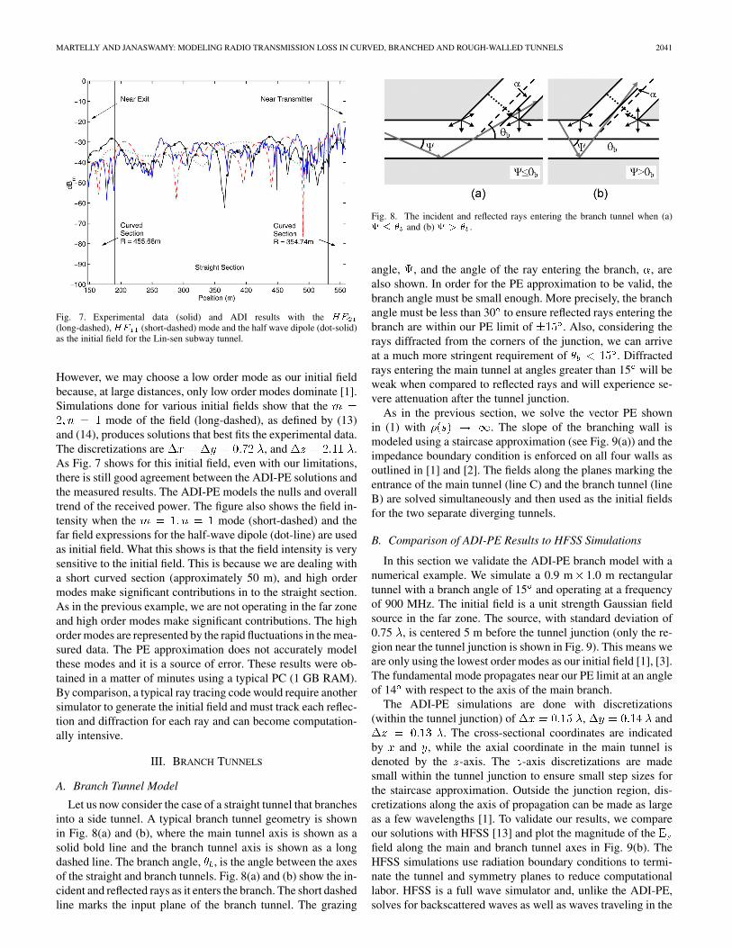
MARTELLY AND JANASWAMY: MODELING RADIO TRANSMISSION LOSS IN CURVED, BRANCHED AND ROUGH-WALLED TUNNELS 2041
Fig. 7. Experimental data (solid) and ADI results with the ��
(long-dashed),�� (short-dashed) mode and the half wave dipole (dot-solid)as the initial field for the Lin-sen subway tunnel.
However, we may choose a low order mode as our initial fieldbecause, at large distances, only low order modes dominate [1].Simulations done for various initial fields show that the
mode of the field (long-dashed), as defined by (13)and (14), produces solutions that best fits the experimental data.The discretizations are , and .As Fig. 7 shows for this initial field, even with our limitations,there is still good agreement between the ADI-PE solutions andthe measured results. The ADI-PE models the nulls and overalltrend of the received power. The figure also shows the field in-tensity when the mode (short-dashed) and thefar field expressions for the half-wave dipole (dot-line) are usedas initial field. What this shows is that the field intensity is verysensitive to the initial field. This is because we are dealing witha short curved section (approximately 50 m), and high ordermodes make significant contributions in to the straight section.As in the previous example, we are not operating in the far zoneand high order modes make significant contributions. The highorder modes are represented by the rapid fluctuations in the mea-sured data. The PE approximation does not accurately modelthese modes and it is a source of error. These results were ob-tained in a matter of minutes using a typical PC (1 GB RAM).By comparison, a typical ray tracing code would require anothersimulator to generate the initial field and must track each reflec-tion and diffraction for each ray and can become computation-ally intensive.
III. BRANCH TUNNELS
A. Branch Tunnel Model
Let us now consider the case of a straight tunnel that branchesinto a side tunnel. A typical branch tunnel geometry is shownin Fig. 8(a) and (b), where the main tunnel axis is shown as asolid bold line and the branch tunnel axis is shown as a longdashed line. The branch angle, , is the angle between the axesof the straight and branch tunnels. Fig. 8(a) and (b) show the in-cident and reflected rays as it enters the branch. The short dashedline marks the input plane of the branch tunnel. The grazing
Fig. 8. The incident and reflected rays entering the branch tunnel when (a)� � � and (b) � � � .
angle, , and the angle of the ray entering the branch, , arealso shown. In order for the PE approximation to be valid, thebranch angle must be small enough. More precisely, the branchangle must be less than 30 to ensure reflected rays entering thebranch are within our PE limit of . Also, considering therays diffracted from the corners of the junction, we can arriveat a much more stringent requirement of . Diffractedrays entering the main tunnel at angles greater than 15 will beweak when compared to reflected rays and will experience se-vere attenuation after the tunnel junction.
As in the previous section, we solve the vector PE shownin (1) with . The slope of the branching wall ismodeled using a staircase approximation (see Fig. 9(a)) and theimpedance boundary condition is enforced on all four walls asoutlined in [1] and [2]. The fields along the planes marking theentrance of the main tunnel (line C) and the branch tunnel (lineB) are solved simultaneously and then used as the initial fieldsfor the two separate diverging tunnels.
B. Comparison of ADI-PE Results to HFSS Simulations
In this section we validate the ADI-PE branch model with anumerical example. We simulate a 0.9 m 1.0 m rectangulartunnel with a branch angle of 15 and operating at a frequencyof 900 MHz. The initial field is a unit strength Gaussian fieldsource in the far zone. The source, with standard deviation of0.75 , is centered 5 m before the tunnel junction (only the re-gion near the tunnel junction is shown in Fig. 9). This means weare only using the lowest order modes as our initial field [1], [3].The fundamental mode propagates near our PE limit at an angleof 14 with respect to the axis of the main branch.
The ADI-PE simulations are done with discretizations(within the tunnel junction) of , and
. The cross-sectional coordinates are indicatedby and , while the axial coordinate in the main tunnel isdenoted by the -axis. The -axis discretizations are madesmall within the tunnel junction to ensure small step sizes forthe staircase approximation. Outside the junction region, dis-cretizations along the axis of propagation can be made as largeas a few wavelengths [1]. To validate our results, we compareour solutions with HFSS [13] and plot the magnitude of thefield along the main and branch tunnel axes in Fig. 9(b). TheHFSS simulations use radiation boundary conditions to termi-nate the tunnel and symmetry planes to reduce computationallabor. HFSS is a full wave simulator and, unlike the ADI-PE,solves for backscattered waves as well as waves traveling in the
2042 IEEE TRANSACTIONS ON ANTENNAS AND PROPAGATION, VOL. 58, NO. 6, JUNE 2010
Fig. 9. (a) Geometry of the branch tunnel. (b) The axial field intensity of the main tunnel from ADI-PE (solid), HFSS (dashed), the branch tunnel from ADI-PE(asterisk) and HFSS (dashed).
forward direction. The backscattering is seen as fluctuationsin the axial field in Fig. 9(b) near the diverging tunnels. Thedielectric constant and conductivity of the tunnel walls is 5 and0.1 S/m, respectively. A high conductivity is chosen so thereis appreciable loss in the small tunnel dimensions allowed inHFSS. As we can see from Fig. 9(b), there is strong agreementin the axial field intensity along the main and branch tunnelaxes between the ADI-PE and HFSS. The figure also showsthere is about a 10 dB drop when going from the main to thebranch tunnel (at the point marked C in Fig. 9(b)). Althoughthe ADI-PE is used to simulate a tunnel with a relativelysmall electrical cross-section (2.7 3 ), it is capable ofhandling larger tunnels at higher frequencies without runninginto memory problems on an average (2 GB RAM) PC [1].
IV. ROUGH-WALLED TUNNELS
A. Rough-Walled Tunnel Model
So far we considered only tunnels with smooth walls, but inthis section we investigate the effects of surface roughness. Sur-face roughness is the local variation of the tunnel wall relative toa mean surface level [4], [5]. In this study we consider randomsurface deviations in an otherwise smooth wall. For the purposeof numerical computations we assume the random deviations tobe Gauassian distributed. A Gaussian distribution of the surfacelevel can be characterized by a root-mean-square height devi-ation and correlation length, [4], [5]. Smooth tunnels havea typical RMS height deviation of 0.01 m and rough surfaces,such as those found in coal mine tunnels, have a RMS heightdeviation of 0.1 m [4]. The excess loss of the field due toroughness in a rectangular tunnel is given by (18)[4]
(18)
where and are the tunnel dimensions in the and axes,respectively, and is the range. The excess loss is derived bytreating the rough surface as a random process and from raytracing techniques, as outlined in [10] and [4]. Equation (18) is
shown in [4] to agree with experimental data taken for coal minetunnels for frequencies ranging from 200 – 1000 MHz.
In our model, we treat small scale roughness by replacingthe rough surface with a flat impedance surface that producesan equivalent specular reflection coefficient. The equivalentimpedance for horizontal and vertical polarization is shown in(19) and (20), [5]
(19)
(20)
where is the surface impedance of the smooth wall, isthe Gamma function, and is the grazing angle. When takinginto account the effects of roughness, we substitute the surfaceimpedance in (3) with the equivalent impedance of either (19)or (20).
Due to the PE angle limitation of , the maximum slopeangle of the rough surface and the grazing angle must satisfythe following relationship
(21)
where is defined as shown in Fig. 10. As we can see fromFig. 10, the angle of the specular reflection of the incident ray,denoted by , depends on the height deviation of the roughness.The roughness angle is related to the RMS height and correla-tion length by
(22)

MARTELLY AND JANASWAMY: MODELING RADIO TRANSMISSION LOSS IN CURVED, BRANCHED AND ROUGH-WALLED TUNNELS 2043
Fig. 10. The geometry of the rough surface.
TABLE IIIANALYTICAL AND NUMERICAL MAFS FOR THE RECTANGULAR TUNNEL
TABLE IVANALYTICAL AND NUMERICAL MAFS FOR THE CIRCULAR TUNNEL
B. Comparison of Numerical and Analytical Solutions
We consider a rectangular 4.26 m 2.10 m tunnel and a cir-cular tunnel with radius of 2 m. The fundamental mode isused as the initial field of the rectangular tunnel and the funda-mental mode generated by a loop ring excitation is used asthe initial field for the circular tunnel. Both tunnels operate at afrequency of 1 GHz and the dielectric constant and conductivityof the tunnel walls are taken to be 12 and 0.02 S/m, respectively.
Tables III and IV summarize the mode attenuation factors(MAFs), or the loss in dB/km, of the smooth and rough tun-nels with rectangular and circular cross-sections, respectively.In real tunnels, as in our simulations, the lowest order mode willdetermine the MAF over a long distance. We used (18) as ouranalytical loss factor for both the rectangular and circular tunnel.As we can see from (18), the loss due to roughness is a functionof wavelength. To notice an appreciable loss at 1 GHz, we as-sume the walls are as rough as cave walls. Therefore, the RMSheight is 0.1 m (0.33 ) and correlation length is 2.5 m (8.33 )for both tunnels.
The grazing angle of the fundamental mode of the rectangularand circular tunnels is computed using the analytical expres-sions for the propagation constant, (where representspropagation in the positive direction), outlined in [4] and [3].The grazing angle is obtained from plane wave theory by [12]
(23)
and is found to be 4.56 and 5.25 for the rectangular and cir-cular tunnel, respectively. The roughness angle is found to be2.29 from (22), and (21) is satisfied. The ADI is simulatedusing discretizations of , and
Fig. 11. The field intensity for the straight tunnel without roughness (solid), forthe straight-curved-straight case (dashed), and for the straight-curved-straightcase with roughness (dot-line).
for the rectangular tunnel andand for the circular tunnel. As we can see fromTable III, the excess loss due to roughness for the rectangulartunnel is about 7 dB when using either (18) and 6.3 dB whenusing ADI-PE. Simulations using a unit strength Gaussian initialfield (where multiple modes are allowed) withand show much less than 1% difference in MAF.Table IV shows the same close agreement in numerical and the-oretical excess loss for the tunnel with circular cross-section.In this case, the excess loss due to roughness is about 16 dB.The accuracy of the results suggests that the equivalent surfaceimpedance, along with ADI-PE, is an adequate model for de-termining loss due to surface roughness. For completeness, welook at the case of the curved tunnel with roughness. Fig. 11shows the field intensity for the rectangular tunnel for thestraight smooth case (solid), the curved smooth case (dashed)and the curved case with roughness (dot-line) with a radiusof curvature of 1800 m. The curved section is in between twostraight sections marked off by two vertical lines. The MAF ofthe curved section with roughness is about 37.7 dB/km. Tunnelswith this type of configuration represents a topic of possible fu-ture work.
C. Comparison of the ADI-PE to Experimental Data
In this section, we examine a real underground tunnel withrough walls and a curving axis. The tunnel is approximately3 m 3 m and the walls are characterized by ,
and with side wall roughness of[11]. The transmitter is placed at the entrance 1.71 m above theground and the receivers are 2.73 m above the ground and op-erate at a frequency of 2.4 GHz. The data was recorded at everymeter along the length of the tunnel. The curvature of the tunnelaxis is shown in the boxed region in Fig. 12. The experimentaldata, shown as the solid line, was provided by the research teamof Moutairou et al. [11].
The numerical simulations were done by computing the radiiof curvature as a function of the tunnel axis and applying rough-ness for the side walls. A unit strength Gaussian with

MARTELLY AND JANASWAMY: MODELING RADIO TRANSMISSION LOSS IN CURVED, BRANCHED AND ROUGH-WALLED TUNNELS 2045
Ramakrishna Janaswamy (F’03) received thePh.D. degree in electrical engineering from theUniversity of Massachusetts, Amherst, in 1986.
From August 1986 to May 1987, he was anAssistant Professor of electrical engineering atWilkes University, Wilkes Barre, PA. From August1987-August 2001 he was on the faculty of theDepartment of Electrical and Computer Engi-neering, Naval Postgraduate School, Monterey, CA.In September 2001, he joined the Department ofElectrical and Computer Engineering, University of
Massachusetts, Amherst, where he is a currently a Professor. He is the authorof the book Radiowave Propagation and Smart Antennas for Wireless Commu-nications, (Kluwer Academic Publishers, November 2000) and a contributing
author in Handbook of Antennas in Wireless Communications (CRC Press,August 2001) and Encyclopedia of RF and Microwave Engineering (Wiley,2005). His research interests include deterministic and stochastic radio wavepropagation modeling, analytical and computational electromagnetics, antennatheory and design, and wireless communications.
Prof. Janaswamy is a Fellow of IEEE. He was the recipient of the R. W.P. King Prize Paper Award of the IEEE TRANSACTIONS ON ANTENNAS AND
PROPAGATION in 1995. For his services to the IEEE Monterey Bay Subsection,he received the IEEE 3rd Millennium Medal from the Santa Clara Valley Sec-tion in 2000. He is an elected member of U.S. National Committee of Interna-tional Union of Radio Science, Commissions B and F. He served as an AssociateEditor of Radio Science from January 1999-January 2004 and as an AssociateEditor of the IEEE TRANSACTIONS ON VEHICULAR TECHNOLOGY.