Embed Size (px)
Citation preview

Report # 2018-06
Processing and inversion of SkyTEM data leading to a hydrogeological interpretation of the Peace River
North Western Area
Client: Geoscience BC
Peace River North-Western Area
In cooperation with
December 23, 2017

Report 2018-06 North-Western area, Phase 1 2
TableofContents
1. EXECUTIVE SUMMARY ............................................................................... 3
2. INTRODUCTION ............................................................................................ 5
3. THE SKYTEM SYSTEM................................................................................. 6
4. DATA PROCESSING ..................................................................................... 7
5. INVERSIONS ................................................................................................11
6. COMPARISON WITH ANCILLARY DATA ....................................................13
7. HYDROGEOLOGICAL INTERPRETATION ..................................................15
8. COMMENTS ON RESULTS .........................................................................25
9. MAPS ............................................................................................................26
APPENDIX 1 (CROSS SECTIONS) .................................................................27
APPENDIX 2 (LIST OF DELIVERABLES) .......................................................37

Report 2018-06 North-Western area, Phase 1 3
1. Executive summary
This study is part of the Peace Project. The Peace Project is a collaborative effort involving Geoscience BC, the Ministry of Forests, Lands and Natural Resource Operations, the Ministry of Environment, the BC Oil and Gas Commission, the Ministry of Natural Gas Development, BC Oil and Gas Research and Innovation Society (BC OGRIS), Progress Energy Canada Ltd., and ConocoPhillips Canada, with additional support from the Peace River Regional District and the Canadian Association of Petroleum Producers. The authors of this report acknowledge the in-kind and funding support these partners have made to this study, through their contributions to the Peace Project.
This report covers the processing, inversion and (hydro)geological interpretation of the SkyTEM data over a portion of the entire SkyTEM survey acquired in the Peace Project. More specifically, it contains results covering the Peace River “North-Western” area.
The AEM and navigation data were first re-processed, starting from raw data, adopting state of the art methodologies aimed at reducing artefacts in the data, and therefore in the derived models. They were then inverted to 3D resistivity models using both Laterally and Spatially Constrained Inversions. Preliminary inversion results were analyzed against ancillary information and provided feedback for data post-processing and final inversions. An extensive set of high-resolution maps of electrical resistivity slices (1:50.000 scale) at different elevations and depths has been provided. The resulting 3D model was then correlated to known geological information to produce a hydrogeological model.
From a geophysical standpoint, the main results of this study include: spatial variability of the resistivity models reflecting potential changes in geology, both near surface and at depth; excellent fit between measured and modelled data, independent of geology or flight lines; seamless models, despite the data were acquired under varying conditions and over a period of several weeks; depth of investigation exceeding, in places, 300 m; effective removal of potential canopy effects; good correlation with depth to bedrock inferred from boreholes.
The derived qualitative geological interpretation highlights: differentiation of different facies within the glacial cover (e.g., resistive glaciofluvial deposits versus the more conductive glaciolacustrine deposits); confirmation of several near surface resistive features associated with paleovalleys and/or areas of thick Quaternary cover identified by previous studies of borehole data; presence of other near surface resistive features that could be of hydrogeological relevance; clear conductive response of the shale bedrock formations (Sully and Buckinghorse); predominantly resistive response of the sandstone Dunvegan bedrock formation; inconsistent response of the predominantly sandstone Sikanni bedrock formation (variability of the sandstone responses might be due to inhomogeneous grain size or water quality); presence of resistive units, in places, at the bottom of the Buckinghorse formation; presence of deep (in excess of 200 m) features with geological continuity, extending over significant distances.
The detailed hydrogeological interpretation and 3D modelling is mainly focused on buried palaeovalleys, which represent the most promising potential for sustainable groundwater production in the area. Some of those valleys were likely formed as tunnel valleys containing enclosed depressions that may be filled with coarse-grained material. At least two generations of valleys seem to be present separated by a widespread glaciolacustrine unit and fluvial sediments. These units, together with the older bedrock units, are included in a 3D model. Although only constructed for a small portion of the entire survey area, this model can potentially be used for planning future groundwater modelling.

Report 2018-06 North-Western area, Phase 1 4
Andrea Viezzoli and Antonio Menghini
Aarhus Geophysics Aps
Fleming Jørgensen and Anne-Sophie Høyer
GEUS-Department of Groundwater and Quaternary Geology Mapping
Geoscience BC is an independent, non‐profit organization that generates earth science in collaboration with First Nations, local communities, government, academia and the resource sector. Our independent
earth science enables informed resource management decisions and attracts investment and jobs. Geoscience BC gratefully acknowledges the financial support of the Province of British Columbia.

Report 2018-06 North-Western area, Phase 1 5
2. Introduction
This report is based on data delivered by SkyTEM Aps on behalf of Geoscience BC and processed and inverted by Aarhus Geophysics Aps. The following hydrogeological interpretation was led by GEUS (the Geological Survey of Denmark and Greenland). The data were collected using a SkyTEM 312 Fast airborne geophysical survey carried out in British Columbia (Canada) in 2015, covering a total of approximately 21,000 line km.
The new processed dataset consists of approximately 4500 line kilometres of AEM data, located in the North Western part of the Peace River Project (Figure 1).
Figure 1. The red polygon outlines the North-Western area. Adapted from Petrel Robertson, 2015.

Report 2018-06 North-Western area, Phase 1 6
3. The SkyTEM system
SkyTEM is a time-domain helicopter electromagnetic system designed for hydrogeophysical, environmental and mineral investigations. The system is shown in operation in Figure 2. The SkyTEM system is carried as an external sling load independent of the helicopter. The transmitter, mounted on a lightweight composite frame in an eight-sided polygon configuration, is a twelve-turn 337 m2 eight-sided loop divided into segments for transmitting a low moment (LM) in two turns and a high moment (HM) in all 12 turns. The LM is about 5.9 A with a turn-off time of 18 s; the HM transmits in the range of 120 A and has a turn-off time ranging from 320 s. This yields a maximum magnetic moment of approximately 490.000 Am2. The z-component receiver loop is placed approximately 2 m above the frame in what is practically a position of null primary magnetic field. Two lasers placed on the frame measure the distance to terrain continuously and two inclinometers measure the tilt of the frame. Power is supplied by a generator placed between the helicopter and the frame.
Figure 2. SkyTEM 312 Fast system.
Measurements are carried out continuously while flying. Every single transient is stored in a binary format, and pre-stacked. Measurements cover the time span from approximately 4.7 µs to 11.4 ms (centre times) from end of ramp. Refer to SkyTEM’s report (Geoscience BC, 2016) for a detailed description of the gate times.
Altitude, TEM data and a number of instrument parameters are monitored and stored digitally so that they can be used for quality control during the data processing stage.

Report 2018-06 North-Western area, Phase 1 7
4. Data processing
The aim of advanced data processing is to prepare data for the inversion. This includes data import, data corrections, filtering and culling and discarding of distorted or noise-affected data. The remaining data are then averaged spatially using trapezoid filters of an optimal configuration, which allows increasing signal to noise level without compromising lateral resolution. Figure 3 shows the schematic block-diagram of the processing and inversion workflow. The processing is carried out using the SkyTEM module of the Aarhus Workbench software package.
Figure 3. Workflow for the data processing and inversion of SkyTEM data carried out with the Aarhus Workbench.
All data are marked with a time stamp, which links transmitter current, altitude, GPS coordinates, etc. During the processing a running mean is calculated separately for the X and Y direction tilt data while algorithms are used to automatically filter out bad altitude data - typically reflections from tree or bush tops.
Reports including QC maps, average resistivity maps, cross sections of multi and few layers,

Report 2018-06 North-Western area, Phase 1 8
In this survey, by virtue of the Primary Field Compensation (PFC) performed by SkyTEM, the first usable time gate in the low moment is around 2.5 s (gate 9) after the end of transmitter “ramp down”.
The processing of voltage data is carried out in a two-step module, featuring automatic and manual modes. The navigation data is corrected for the transmitter/receiver tilt, and altimeter drops, while for the EM data other filters are employed which are designed to cull coupled or noise influenced data. Note: in order to preserve the integrity of the measured data, the processing is carried out on the raw data in binary format, rather than on the pre-filtered ASCII data.
In the next step, the automatically processed raw soundings are inspected visually using a number of different data plots. At this stage it is assessed whether the filters have removed the right amount of data coupled to man-made infrastructures. It is usually necessary to intervene manually to fine-tune the outcome of the filters and obtain the most reliable results. Figure 4 shows a view into the data processing module of the Aarhus workbench over a section of SkyTEM data from another survey, with data culled due to coupling with man-made structures.
Figure 4. The data processing window of the Aarhus Workbench, showing portions of data deleted because of coupling with man-made structures (top) and of random background noise (bottom).
Altimeter data are also assessed and edited, since an erroneous measure of ground clearance used as input to the inversion can produce artefacts in the resistivity models. The aim of altimeter filtering is to remove laser reflections, which are not coming from the ground, such as reflections from tree tops. This procedure is carried out with an algorithm, which is based on the fact that the reflections from the treetops result in lower apparent flight altitude, than the other reflections. The algorithm filters out the data by repeatedly making a polynomial fit to the data and then by removing data some meters below the latest polynomial fit. This automatic filtering is followed

Report 2018-06 North-Western area, Phase 1 9
by a manual inspection and in some cases manual refinements. This procedure is mostly needed in areas with very few ground reflections. In such areas, it can be advantageous to calculate another flight altitude based on the above sea level altitude from the GPS and a digital elevation model. While less accurate than the flight altitude based on the laser reflections from the ground, this flight altitude can be used to guide the manual refinements. Figure 5 shows an example of processing of laser altimeter data.
Figure 5. Example of processed laser altimeter data (brown line) versus raw measured data (green and red dots) in an area with canopy cover.
EM data are further averaged to increase the signal to noise ratio using a trapezoid shaped averaging core, where the averaging width of late time data is larger than that of early time data, as shown in Figure 6.
Figure 6. The principle behind the trapezoid shaped averaging core where data are averaged over larger time spans at later times to maintain as much lateral resolution as possible at early times while keeping a high penetration depth.
The data uncertainty for these stacked (averaged) soundings is calculated from the data stack. Furthermore, a minimum small uniform (or “floor”) data uncertainty is assigned to all data. For the current study, this floor uncertainty has been set to 3%.
Width1
Width2
Width3
t
Flight time
Gate 1
Gate 2
Gate n
Gate 3
Sounding
T2
T1
T3

Report 2018-06 North-Western area, Phase 1 10
Soundings were produced for every 1.4 s corresponding to approximately 30 m distance from one another. The good signal levels recorded in large portions of the survey, allowed using trapezoid averaging filters of moderate width. Table 1 provides a summary of the automatic filters applied to the dataset.
LM HM
Distance between averaged soundings (s) 1.4 1.4
Time of first trapezoid knee point (T1) 1e-5 1e-4
Time of second trapezoid knee point (T2) 1e-4 1e-3
Time of third trapezoid knee point (T3) 1e-3 1e-2
Width of first trapezoid section (width 1) 3 3
Width of second trapezoid section (width 2) 5 5
Width of third trapezoid section (width 3) 8 10
Table 1. The settings for the automated filters employed in the first part (automatic filtering) of the processing, for the low (LM) and high (HM) moment of the SkyTEM system. All the above times are expressed in seconds.
After the automatic stacking, soundings are inspected visually using a number of different data plots. At this stage it is assessed whether data points at late times should be ascribed a higher uncertainty or removed entirely. It is customary to cull data when the background noise level reaches the level of the earth response. Assessing data for usability is done by inspecting the decay curves, the distance to potential noise sources and the level of the background noise.
This process is necessary to gain reliable model parameters in all parts of the data sections. Figure 7 shows one averaged sounding (transformed into a version of late time apparent resistivity), with different time gates displaying different noise levels, for low and high moment. These curves (not normalized with Tx current) are used only for data editing.
Figure 7. Example of averaged sounding (transformed into late time apparent resistivity), with different time gates displaying different noise levels, for low and high moment.

Report 2018-06 North-Western area, Phase 1 11
5. Inversions
Preliminary inversions are carried out using the quasi 2-D Laterally Constrained Inversion (LCI). Final inversions are carried out using the quasi 3-D Spatially Constrained Inversion (SCI). LCI and SCI are full non-linear damped least squares solutions in which the transfer function of the instrumentation is modelled. This includes, among other things, current turn-on and -off ramps, front gate and low pass filters, system altitude, etc. The inversion kernel is “AarhusInv”, designed by the University of Aarhus. This code performs efficient large-scale inversions and is crucial for testing inversions as well as examining the model space. Figure 8 shows a sample from the geometry file, describing the SkyTEM system used in this project.
Figure 8. Sample of geometry file used to describe the SkyTEM system when modelling FWD responses. Preliminary LCIs served the purpose of fine tuning the post-processing of the EM data, in terms of both couplings and noise assessment.
In the SCI scheme the model parameters are tied together spatially with a spatially dependent covariance, which is scaled according to the distance between neighbouring stations. Constraining the parameters tends to enhance the resolution of resistivities and layer interfaces, which are not well resolved in an independent inversion of the soundings. The flight altitude is included as an inversion parameter with a prior value calculated from the tilt corrected laser altitudes. The standard deviation on this parameter is set to 1 m.
The SCI inversion scheme is developed using 30 layers (each layer having a fixed thickness and varying resistivity). Regularization (incorporating our a-priori knowledge or assumptions) consists

Report 2018-06 North-Western area, Phase 1 12
of a vertical smoothing constraint term (smooth inversion) applied to stabilize the inversion, e.g. to remove fictitious layers especially in models based on few data points. The lateral constraints, which get tighter for deeper layers, were set on absolute elevation (rather than on depth), due to the geological settings of the area, which suggests greater degree of continuity of electrical resistivity within the same absolute elevation intervals.
The depth of investigation (DOI), based on an analysis of the Jacobian matrix, was also calculated for the output models. This DOI, is presented in a dedicated horizontal map, as well as superimposed to crop the average resistivity horizontal maps, and as a fading of colours below the DOI on the vertical cross sections. The DOI represents the maximum depth below surface to which there is little or no sensitivity to the model parameters. Any model parameter resting much below the DOI should be disregarded. For example, the DOI often rests at, or close to, an interface between a conductive overburden and a resistive deeper layer. In this case we can conclude that the conductive layer does end at that interface, and it rests above a significantly more resistive layer, whose absolute resistive value is poorly determined.
The multi-layered model uses fixed thicknesses discretized into 30 layers; however the resistivity value of each layer remains a free parameter to be fit during the inversions. It was discretized to 400 m, with layers logarithmically increasing in thickness, with the upper most (shallow) layer starting at 3 m. Dozens of preliminary inversions were carried out, carefully fine tuning the settings of regularization, convergence, DOI, uncertainties. Table 2 below summarizes the main settings (homogeneous at all depths) of the final SCI. The vertical constraints are purposely left loose, in order to allow sharp vertical variations in the resistivity models.
A higher halfspace resistivity was used for the starting model of the North Western corner of the area, where the bedrock is mainly formed by limestones and dolomites.
Resistivity starting model (ohm-m) 40 in general (100 for the NW corner)
Vertical Constraints 3 (with exception of first layer, =2)
Lateral Constraints 1.3
Reference distance (m) 40
Power law distance drop off 0.5
Table 2. SCI settings.
A number of boreholes provided by the client describing depth and type of bedrock were inspected and used for comparison with inversion results (cfr Section 6). However they were deemed not suitable to be used as extra input to the inversions, as a-priori, due to both their localized nature and the lack of downhole resistivity measurements. It is expected that if and when data describing physical properties of the subsurface becomes available (e.g., shallow seismic), they could be incorporated to refine the local inversions, and ultimately the interpretation.
The inversion results are presented as a series of both horizontal and vertical slices.The maps of average resistivity at different horizontal intervals are given in elevation above mean sea level. All models are masked by DOI and shown with corresponding data fit.

Report 2018-06 North-Western area, Phase 1 13
6. Comparison with ancillary data
The inversion results obtained in this study were compared against three different types of ancillary data. In section (6.1) a number of boreholes describing depth and type of bedrock were inspected and used for comparison with resistivity cross-sections. The inversion results were then assessed in plan view (6.2) against maps of paleo valleys and isopachs of Quaternary sediments (Hayes et al., 2015).
The following simplified hydrogeological settings are considered. The Quaternary sediments comprise the unconsolidated cap, typically no more that 15m in thickness. This overburden is of varying origin; namely, glacio-fluvial deposits (sands, pebbles and gravels), glacio-lacustrine deposits (silty clays or clayey silts), and tills. Moreover, there can be admixtures of colluvial (sandy and clayey silts) and fluvial units (mainly sands and gravels) generally limited to the existing river valleys, but sometimes related to pre-existing river channels. The underlying bedrock is comprised of Cretaceous-aged shale and sandstone formations, namely, the Dunvegan (sandstones and conglomerates), Sully (shales and siltstones), Sikanni (sandstones) and Buckinghorse (shales). Two geological formations were added, which had not been encountered in the previous projects: Lower Buckinghorse (most likely shales) and Nordegg (calcareous mudstones). The former seems to display a higher resistivity than the Buckinghorse (see Section in Figure A3) but we do not have enough data to confirm this behaviour. On the contrary, Nordegg has a clear resistive response, even though influenced by degree of fracturing and other possible local variations.
6.1. Comparison of cross-sections of inversion results against boreholes
Several vertical cross sections are provided in Appendix 1. Figures A2 to A6 display a selection of vertical resistivity sections overlain by simple borehole information, i.e., thickness of Quaternary sediments, depth to and type of bedrock. Profiles locations are shown in Figure A1.
These sections
a) do not coincide with individual flight lines, but rather connect boreholes
b) do not interpolate the resistivity models, but rather the actual resistivity models are projected onto the profiles from a maximum distance of 200 m.
The borehole data, on the other hand, are projected from a maximum distance of 500 m.
From a purely geophysical standpoint, the inverted resistivity models display satisfactory misfit, and significant Depth of Investigation, ranging in the order of 200 m to 300 m.
The models recover depth to bedrock with good accuracy, both shallow, within the majority of the area, and in the few instances where paleovalleys cut deeper into it. Some formations (e.g., Sully) show consistent resistivity responses, while others (e.g., Sikanni and Dunvegan) vary. This can be due either to water quality variations, local inhomogeneities (facies variations) in the rock matrix or both. The Quaternary units also display a degree of lateral variations in resistivity, probably due to the presence of glaciolacustrine deposits.
As will be examined in detail in the next section, some resistive structures within the Quaternary coverage were considered potential buried valleys filled with gravels and sands; they could have interest from a hydrogeological point of view, as they could represent exploitable aquifers.
The qualitative interpretation of the resistivity sections in Figures A2 to A5 is based on the integration of borehole data and previously known stratigraphic information (the formations accompanied by question marks). These qualitative interpretations provided the building blocks for further integrated studies and more advanced hydrogeological modelling.
Provided that a more detailed discussion about the Quaternary setting, especially about buried valleys and glacial deposit features, will be treated on the next chapter, the cross-sections confirm complicated pattern of bedrock formations: we can recognize huge plicative deformations, with

Report 2018-06 North-Western area, Phase 1 14
the definition of anticlines and synclines. The general response of the main formations is well confirmed: mainly resistive for Dunvegan and Sikanni, clearly conductive for Sully and Buckinghorse. Even though outside the scope of this project, we note that the Lower Buckinghorse unit seems to display a more resistive response, and might represent a potential hydrocarbon exploration target worth following up.
Several more buried valleys are recognizable beside the ones treated in the geological modelling. They display a complex geometry with very thick resistive buried valleys (reaching depths of 100 m and more), sometimes separated by conductive glacio-lacustrine lenses. The main structures are located along the Halfway River.
6.2. Comparison of horizontal sections of inversion results against known geology
Maps 1.RHO.005, 1.RHO.010, 1.RHO.015 and 1.RHO.020 (see Appendix 2 for details) display slices of near surface resistivity, obtained from SCI, plotted over surface geology. The resistivity models show a large degree of spatial variability. Exposed bedrock in the eastern portion of the area correlates well with conductive features. Some resistive features are in reasonable agreement with outlines of paleo-valleys and thick Quaternary aquifers inferred from the borehole data (reinterpreted gamma logs), while other features do not correlate.
A discussion about some selected resistivity maps is reported in Appendix 1.
Resistivity maps at intermediate depths display many other features worthy of consideration. Refer to the files containing a complete overview of resistivity slices at different elevations and depth intervals.

Report 2018-06 North-Western area, Phase 1 15
7. Hydrogeological interpretation 7.1 General interpretation of bedrock
A preliminary geological interpretation has been undertaken for the entire dataset in the North Western area. The geological interpretation of this area is consistent with the interpretation of the area to the Southeast (Jørgensen et al. 2016). The northwesternmost part of the area, around Pink Mountain, older formations are present. These comprise the Monteith and the Gething Formations as well as very resistive limestones of the Triassic. Also the Nordegg formation is included into this stratigraphic succession. These formations are heavily deformed in this region and also excavated where the Halfway River crosses Pink Mountain (Hinds & Cecile et al. 2003).
Apart from the Pink Mountain area, the lithostratigraphic formations within the penetration depths of the SkyTEM method are from below: (i) the Buckinghorse Formation (shales, silty mudstones and siltstones), overlain by, (ii) the Sikanni Formation (alternating layers of sandstone, siltstone and shale), (iii) the Sully Formation (mainly shales and siltstones) and finally topped by (iv) the Dunvegan Formation (sandstones and conglomerates). According to electrical logs the Sikanni Formation has a resistivity value between 15-20 ohm-m, the Sully Formation between 10-15 ohm-m, and the Dunvegan Formation shows resistivities between 15 and 50 ohm-m. The Dunvegan Formation constitutes the uppermost bedrock in the study area.
The geological interpretation is shown on two representative cross sections. The location of the cross sections is shown in Figure 9. Estimated thrust faults are delineated with thick red dotted lines and inferred bedrock formation boundaries are delineated by thick grey lines. Interpretations in the drift succession are delineated by thin black dotted lines. The cross sections are shown in Figure 10.

Report 2018-06 North-Western area, Phase 1 16
Figure 9: Elevation map of study area with location of cross sections (pink lines), 3D model area (blue polygon), mapped buried palaeovalleys (black lines).

Report 2018-06 North-Western area, Phase 1 17
Figure 10: Cross sections with geological interpretations. Estimated thrust faults are delineated with thick red dotted lines and inferred bedrock formation boundaries are delineated by thick grey lines. Interpretations in the drift succession are delineated by thin black dotted lines. The DOI is shown with a thin grey dotted line. Location of cross sections is shown in Figure 9. Vertical exaggeration 10x.
In the deeper part of the cross sections to the NE and at shallow to medium depths towards the SW, a thick unit of medium to low resistivity is recognized. This unit is interpreted as a clay-rich succession corresponding to the Buckinghorse Formation. The interpretation of the lower boundary of this unit is very uncertain, since it seems to be situated below or approximately at the same level as the DOI. In the northeastern part of the sections the upper boundary is also hard to estimate. Here it is due to large depths and the presence of the conductive Sully Formation above. Since the Buckinghorse Formation is difficult to penetrate, the thickness of the formation is difficult to estimate. What is below the Buckinghorse has therefore not been interpreted.
Above the Buckinghorse, an up to 200 m thick, more resistive unit is recognized. This is interpreted as the Sikanni Formation where the sandy parts make the unit more resistive compared to the Buckinghorse Formation. These two units are clearly thrusted and folded with the thrust faults dipping towards the NE. On top of the Sikanni Formation, an up to 150 m thick, conductive unit follows. This unit corresponds to the clay-rich lagunal deposit of the Sully Formation. The generally resistive layers present at high elevations on the mountain tops, and above the Sully Formation is interpreted as the Dunvegan Formation. The heterogeneous resistivity pattern in this formation reflects the interbedding with conglomerates, shale and coal.
The main structural features dominating the cross sections are an anticline/thrust at 22,000 m in Profile A and at 14,000 m in Profile B. Towards the Southwest this is followed by synclines. One large syncline in Profile A (app. 13,000 – 20,000 m) contains a huge body of the Sikanni sandstone. The next syncline is seen on both profiles and this is where the Halfway River flows (app. 5,000 – 12,000 m on Profile A). A considerable succession of drift sediments is found along this valley and its western tributaries.
The geological interpretations of the bedrock are outlined on a selected horizontal resistivity slice (see Figure 11, and Appendix 1).

Report 2018-06 North-Western area, Phase 1 18
Figure 11: Horizontal resistivity slice at 765 m above sea level. The major geological formations are outlined.
7.2 Buried valleys/palaeovalleys
Special attention has been placed on buried valleys, especially within and in the vicinity of the Halfway River valley where their occurrence seems to be more frequent than in the rest of the study area. A number of buried valleys have been mapped, see Figure 9. They are seen in the resistivity data as elongate resistive structures that broadens upwards through the resistivity model.
These buried valleys occur in at least two generations. The first generation is situated below an extensive unit of glaciofluvial sediments and glaciolacustrine clay found in large parts of the Halfway River valley and its tributaries. The second generation seems to be younger, cutting down into the glaciofluvial and glaciolacustrine units and into the first generation of buried valleys (see Figure 10).
The first generation of buried valleys have overdeepened sections along their thalwegs and may therefore be interpreted as subglacially formed tunnel valleys that are now buried by younger sediments. Tunnel valleys are cut into the subsurface at the glacier bed by pressurized meltwater. Such type of buried valleys are frequently found within all formerly glaciated areas (e.g. Jørgensen and Sandersen 2006). In geometry the valleys resemble the ones mapped with AEM in other parts of the world, we thus interpret the valleys as tunnel valleys.

Report 2018-06 North-Western area, Phase 1 19
The formation of the second generation of buried valleys is connected to recent, and eventual pro-glacial, fluvial erosion. Those buried valleys are limited in depth and are found beneath many stretches of modern rivers, such as the Halfway River and its tributaries.
The extensive unit of glaciofluvial sediments and glaciolacustrine clay found between the two generations of valleys is well known from outcrops and geological maps (Petrel Robertson 2015). Especially the upper part, which is a clay rich glaciolacustrine clay, is well resolved in the SkyTEM data. In the SkyTEM data it is seen as a thin conductive layer. The outwash sediments below have high resistivities.
Two long tunnel valleys seem to occupy the lower part of the drift succession along the Halfway River valley. One of these can be followed from the southernmost part of the area until where the Chowade River branches, see Figure 9. Here it bends towards the West and follows the Chowade River valley. A cross section along the thalweg of the valley is shown in Figure 12. The tunnel valley seems to be more than 100 m deep at its deepest depressions. Since the valley fill becomes more conductive with depth it appears to be getting more fine-grained in the deeper parts. The outwash unit on top, however, is very resistive indicating coarse-grained sediments.
Figure 12: Cross section from north (left) to south (right) along the thalweg of the long tunnel valley following the southern part of the Halfway River valley in the study area. The grey lines indicate interpretations of the valley and the layers above. Note the undulating bottom profile. The valley fill seems to be more conductive with depth indicating more clayey sediments in the deeper part.
The second long tunnel valley is found beneath the northernmost stretches of the Halfway River valley (Figure 9). It can be followed until it crosses Pink Mountain in the far North. This valley is up to about 75 m deep in its northern part (see Figure 13). These valleys have subsequently been cut by modern river streams along large sections of their length and in these sections it is difficult to distinguish between the modern river sediments and the older tunnel valley fill. The uncertainty of the interpretations is thus relatively high here.
Figure 13: Cross section from north (left) to south (right) along the thalweg of the long tunnel valley following the northern part of the Halfway River valley in the study area. The grey lines indicate interpretations of the valley and the layers above. Note the undulating bottom profile.
7.3 Detailed geological 3D model

Report 2018-06 North-Western area, Phase 1 20
The 3D geological model was constructed using the geological software modelling tool ‘Geoscene3D’ from I-GIS. The model area is situated in the southwest (Fig. 9) and covers an area corresponding to approximately 19 km E-W x 8 km N-S. The model area covers a section of the long tunnel valley that follows the southern part of the Halfway River valley (profile distance 10000m to 18000m in Fig. 12). In the following, this valley is named ‘buried valley 1’. Figure 14 shows a close-up of the surface geology map in the model area together with the outline of the interpreted buried valleys and the position of the profiles in Figures 16 and 17.
Fig. 14: The model area (grey) shown on top of the surface geology map by Petrel Robertson, 2015. Outline of the interpreted buried valleys are shown with blue. Location of the profiles in Figs. 16 and 17 are shown (named ‘flightline N1’ and ‘flightline N13’).
The geological modelling is performed using a combination of layer- and voxel modelling. The bottom of each geological unit is modelled using interpretation points that have been kriged into surface layers. The bottom of four overall stratigraphic boundaries have been modelled; Buckinghorse Fm, Sikanni Fm, Sully Fm and Dunvegan Fm. In the valley, the bottom of 6 Quaternary boundaries have been modelled; Buried valley 1, buried valley 2, buried valley 3 (Fig. 14), the meltwater plain, the modern valley fill and the glaciolacustrine deposits.
Subsequently, a voxel model is constructed by using the tools described in Jørgensen et al. (2013). The final voxel model is discretized with 100 m x 100 m laterally and 5 m vertically and covers the elevation interval from 300 m.a.s.l. (meters above sea level) to the terrain surface (up to 1210 m.a.s.l.), resulting in c. 7.7 million voxels. The voxel model is constructed by selecting and populating voxels within volumes delineated by the modelled layer surfaces and defined regions. Overall, the units correspond to the ones defined by the layer surfaces, but two of the units (‘Buried valley 1’ and the ‘Dunvegan Fm’) are subdivided into lithological facies based on the resistivity values within the units (Table 3). The other Quaternary units are modelled as homogeneous units. The stratigraphic formations are known to be heterogeneous, but due to the greater burial depth of these formations, the SkyTEM data are not able to resolve the small lithological variations and resistivity values are therefore not used for lithological characterization within these units. Consequently, the voxel model consists of 13 categories, which are shown in Figure 15.
Table 3: Subdivision of geological units in the voxel model based on resistivity values within the units.

Report 2018-06 North-Western area, Phase 1 21
Resistivity below 60 ohm-m Resistivity above 60 ohm-m
Buried valley 1 Clayey valley fill Sandy and gravelly valley fill Dunvegan Fm Silty shale Sandstone and/or pebble conglomerate
Fig. 15a,b: 3D view of the model results seen from southeast. 5 x vertical exaggeration, a) 3D view of the voxels, b) E-W and N-S slices through the model shown together with the layer surface outlining buried valley 1. Figure 15 shows 3D views of the model results. East of the valley, a synclinal structure is recognized in the northern part of the model area (Fig. 16), whereas a thrust fault structure is recognized below the Buckinghorse Fm in the southern part (Fig. 17). The Sully and Dunvegan Formations are only present in the southeastern part of the model (Fig. 15).
Quaternary deposits have only been modelled within the modern valley structure (Fig. 15), since the remaining part of the area generally shows a thin cover of Quaternary sediments (Fig. 14) with thicknesses below the vertical discretization in the voxel grid (<5m). In the modern valley structure, the Quaternary deposits have thicknesses between 20m to approximately 250m, where the buried valleys are deepest.
Three buried valleys are modelled within the model area. The largest is the one named ‘buried valley 1’. This corresponds to the southernmost long tunnel valley described in Section 6.2 (Fig. 12), and it is located directly below the modern river in the southern part of the model (Fig. 17, profile distance 9000m). In the north, it is located below an erosional remnant of glaciolacustrine deposits (Fig. 16, profile distance 7700m). The lower part of the valley is mainly filled with clayey deposits, whereas the upper part has coarse-grained infill. Close to the hill-side in the eastern side of the modern valley, buried valley 2 is located and filled with mainly coarse-grained deposits.

Report 2018-06 North-Western area, Phase 1 22
Buried valley 3 is located in the northwestern part of the model area (Fig. 14) and is filled with clayey deposits.
All three buried valleys are interpreted to be first generation tunnel valleys that are older than the meltwater plain. The coarse-grained deposits from this unit therefore cut through the buried valley structures (Figs.15, 16 and 17). Glaciolacustrine clays are modelled on top of the meltwater plain, and in the north, a marked erosional remnant of these glaciolacustrine deposits forms a small hill structure in the middle of the modern valley (Fig. 15, and 16, profile distance 7200-8200m). The youngest deposits in the geological model is the sand and gravel deposits from the modern river bed, which is cut into the underlying deposits (e.g. Fig. 16, profile distance 8800-9800m).
Fig. 16 a,b: a) SkyTEM resistivities and the DOI along the northernmost flightline within the 3D model area (flightline N1 in Fig. 14), b) geological model results along the same profile. 5x vertical exaggeration.

Report 2018-06 North-Western area, Phase 1 23
Fig. 17 a,b: a) SkyTEM resistivities and the DOI along the southernmost flightline within the 3D model area (flightline N13 in Fig. 14), b) geological model results along the same profile. Note that the Dunvegan Fm is subdivided into a clayey and non-clayey fraction. 5x vertical exaggeration.
7.4 Hydrogeological perspectives
Although hydrological data are not available from the area, the interpretation of the new SkyTEM data indicates that the buried valley structures and the covering outwash sediments could represent groundwater reservoir potential. The buried valleys are eroded into the Buckinghorse Formation that mainly consists of shale and mudstone with a low hydraulic conductivity and no groundwater potential.
The infill sediments in the buried valleys show varying resistivities, so the potential most likely also varies within each structure. Even though the meltwater plain and the buried valley 2 are modelled as coarse-grained units, both of these units show varying resistivities from around 40 to 100 ohm-m. Deposits with resistivities below 60 ohm-m are expected to show an increased clay content. The highest resistivities are found within the modern river bed (>100ohm-m), thus indicating coarse-grained sediments without much clay. In many places, the modern river bed is in direct contact with deposits in the meltwater plain and/or the buried valley structures (e.g. Fig. 17, profile distance 8,000 – 9,500m). Due to the direct hydraulic contact between the modern river bed and the possible aquifers beneath, groundwater extraction here could cause a depletion in river flow due to strong groundwater-surface water interaction. The groundwater extraction potential is in many places therefore dependent on the existence of a hydraulic barrier between the aquifers and the river bed. The most interesting sites for groundwater extraction could therefore be within the sand-filled parts of the buried valley structures, or in the meltwater plain, where those units are not in a direct hydraulic contact with the modern river bed.
Outside the 3D model area potential sites for groundwater extraction could be at local deepenings along the buried tunnel valleys, e.g. at distance 11,000 m in the northernmost long tunnel valley (see Figure 13). At this particular site, the tunnel valley is covered by the glaciolacustrine clay and therefore not in close contact with the river. The resistivity of the valley fill decreases when it is covered by conductive glaciolacustrine clay (Figure 13), but this is inferred to be an artifact

Report 2018-06 North-Western area, Phase 1 24
resulting from the inversion: the resistive fill cannot be fully resolved here due to the limited thickness of the layer.

Report 2018-06 North-Western area, Phase 1 25
8. General comments on the EM data processing and inversion results.
The results of the processing and inversion project are overall satisfactory, suggesting a positive outcome of the used techniques.
The processing of the navigation data required careful manual inspection and editing large areas covered by canopy.
The models produced are, to the best of our knowledge, void from significant cultural artefacts. It must however be stated that the lack of information about buried infrastructures added a degree of complexity and uncertainty to the processing of the EM data.
The settings for the final inversions were based on the analysis of several different preliminary realizations, assessed against the relevant ancillary information available. The regularization was chosen to best fit the geological settings of the area, with sharp vertical boundaries and spatial constraints limiting the variance with respect to absolute elevation.
The data misfit (normalized by standard deviation) is generally low (around 1) and homogenous throughout the entire data set, which is indicative of proper discretization, regularization and processing. The Depth of investigation ranges between 200m and 300m. No suitable ancillary data (e.g., pre-existing geological model, or large scale complementary geophysical data) were available to constrain the inversions over large areas. It is anticipated that, e.g., surfaces derived from seismic data, could be incorporated into future inversions to produce refined results.
The results are presented as an entire suite of resistivity maps at different absolute elevation intervals to be more representative of the geological settings. A limited number of near-surface resistivity maps at four depth intervals are also provided, to allow immediate correlation with the maps of depth to bedrock. The resistivity models reflect the significant spatial hydrogeological variability of the area. They are in good agreement with the available ancillary information and prior hydrogeological knowledge, both near surface and at intermediate depth. The models provide new insight into complex local near surface alluvial features as well as into large-scale structures. They also image large structures of geological appearance within bedrock, at depths where no ancillary information is currently available. Overall, the results present a valid base for further data integration and hydrogeological interpretation.

Report 2018-06 North-Western area, Phase 1 26
9. Thematic maps and sections
To visualize the processing and inversion results in the survey area, a number of theme maps and vertical sections were prepared. The colour scale for both average resistivity maps and vertical cross sections is a rainbow colour scale with hot colours representing resistive domain and cold colours representing conductive domain. A complete list of all final deliverables is provided in Appendix 2.
All final maps, except when stated otherwise in the legend, have been made using the kriging method (no nugget, exponential fitting), with a search radius of 1000 m and 30 m node spacing. We now present a brief explanation of the key maps mentioned above, and their use.

Report 2018-06 North-Western area, Phase 1 27
Selected references
Geoscience BC Report 2016-03, SkyTEM Survey: British Columbia, Canada; Data Report.
Geoscience BC Report 2016-04, Petrel Roberston Consulting: Interpretation of Quaternary Sediments and Depth to Bedrock Through Data Compilation and Correction of Gamma Logs.
Hinds, S.J. & Cecile, M.P. (a.o.) 2003: Pink Mountain and northwest Cypress Creek Map areas (94G/2 & NW94B15), scale 1:50 000. Open file geological map, Geological Survey of Canada.
Jørgensen, F. and Sandersen, P.B.E. 2006: Buried and open tunnel valleys in Denmark – erosion beneath multiple ice sheets. Quaternary Science Reviews, Vol. 25, 11-12, pp. 1339-1363.
Jørgensen, F., Møller, R.R., Nebel, L., Jensen, N.-P., Christiansen A.V. and Sandersen, P.B.E. 2013: A method for cognitive 3D geological voxel modelling of AEM data. Bulletin of Engineering Geology and the Environment. Vol. 72, 3, 421-432. DOI: 10.1007/s10064-013-0487-2.
Jørgensen, F., Menghini, A., Kallesøe, A.J., Vignoli, G., Viezzoli, A. & Pedersen, S.A.S. 2016: Structural geology of folded terrain in the Rocky Mountains' foothills interpreted from SkyTEM - A preliminary study of SkyTEM data collected in the Peace region, NE British Columbia, Canada. Danmarks og Grønlands Geologiske Undersøgelse Rapport 2016/34. 21 p.

Report 2018-06 North-Western area, Phase 1 28
Appendix 1
This Appendix contains a few vertical resistivity cross sections and resistivity slice maps, mentioned in Section 6.1.
Figures A2 to A5 display a selection of vertical resistivity sections (W-E) overlaid with simple borehole information, i.e., thickness of Quaternary sediments, depth to and type of bedrock. The location of the profiles are provided in Figure A1. Notice that these section a) do not coincide to individual flight lines, but rather connect boreholes, b) do not show any interpolation of the resistivity models, but rather use the actual resistivity models that are projected onto the profiles from a maximum distance of 200 m. The borehole data, on the other hand, is projected from a maximum distance of 300 m.
Figure A1. Location of cross-sections shown in Figures A2 to A9, overlaying map of surficial geology, buried valleys and thicker sediments inferred from borehole data (adapted from Petrel Robertson, 2015). Boreholes are represented by the black dots.

Report 2018-06 North-Western area, Phase 1 29
Figure A2. Vertical resistivity cross sections P1 (top) and P2 (cfr Figure A1 for location) compared to borehole data (depth to and – color coded- type of bedrock), overlain with preliminary qualitative interpretation of main structures. Distance (m) from drillhole location shown above the boreholes. Models are shaded with DOI and show associated data misfit (black line, to be read against right axis).
Report 2018-06 North-Western area, Phase 1 30
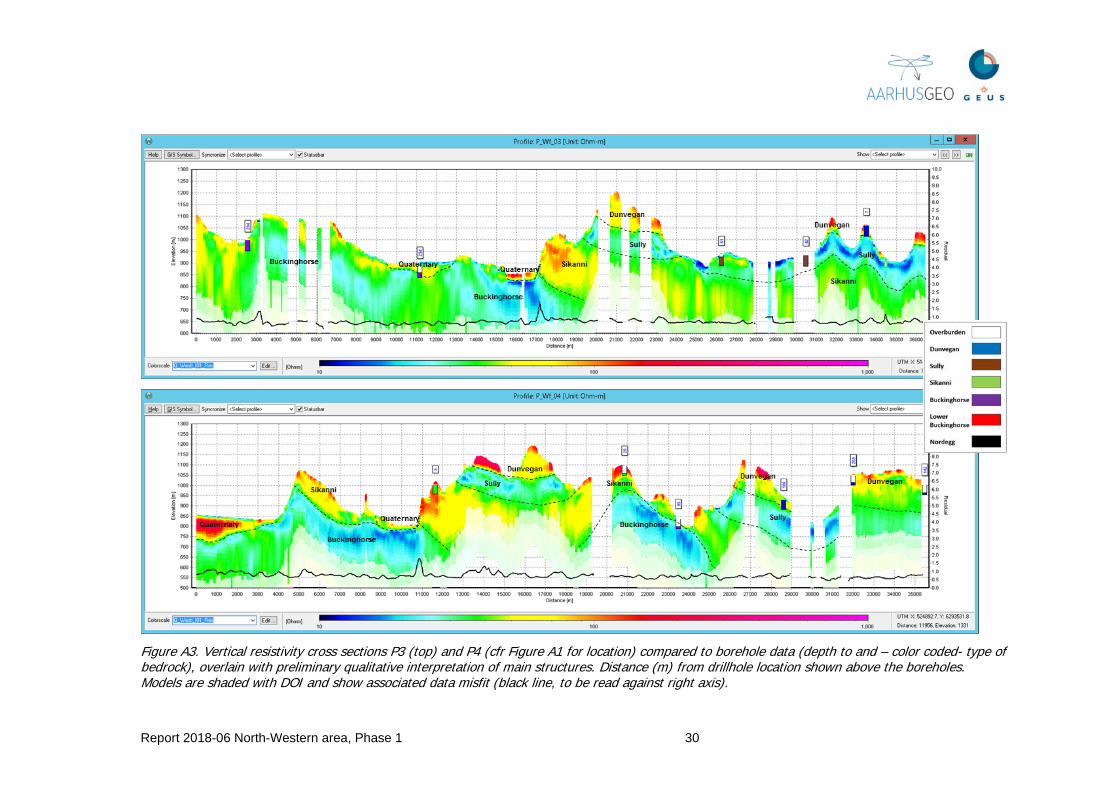
Figure A3. Vertical resistivity cross sections P3 (top) and P4 (cfr Figure A1 for location) compared to borehole data (depth to and – color coded- type of bedrock), overlain with preliminary qualitative interpretation of main structures. Distance (m) from drillhole location shown above the boreholes. Models are shaded with DOI and show associated data misfit (black line, to be read against right axis).

Report 2018-06 North-Western area, Phase 1 31
Figure A4. Vertical resistivity cross sections P5 (top) and P6 (cfr Figure A1 for location) compared to borehole data (depth to and – color coded- type of bedrock), overlain with preliminary qualitative interpretation of main structures. Distance (m) from drillhole location shown above the boreholes. Models are shaded with DOI and show associated data misfit (black line, to be read against right axis).

Report 2018-06 North-Western area, Phase 1 32
Figure A5. Vertical resistivity cross sections P7 (top) and P8 (cfr Figure A1 for location) compared to borehole data (depth to and – color coded- type of bedrock), overlain with preliminary qualitative interpretation of main structures. Distance (m) from drillhole location shown above the boreholes. Models are shaded with DOI and show associated data misfit (black line, to be read against right axis).

Report 2018-06 North-Western area, Phase 1 33
Figures A6 to A10 display a selection of resistivity slice maps. The first one shows the correlation between outcropping geology and shallow resistivity (0-5 m depth), confirming the electrical response of the geological formation. Notice the good resolution of the elongated resistive Quaternary deposit associated to the Halfway River and its tributary Chowade River: they can be associated to buried valleys detected in Section 7. Of course, the resistivity distribution is strongly influenced by topography, hence it is hard to follow geological structures. For this purpose it is better to make use of maps in elevation (m a.s.l.).
Figure A6. Resistivity slice map at depth of 0-5 m.

Report 2018-06 North-Western area, Phase 1 34
Figure A7 is referred to 890-900 m a.s.l. and it is able to distinguish a very interesting resistive feature (a buried valley) within the Quaternary coverage on the Northern and in the Central area. As already evidenced in the previous project, there is a clear N-S pattern of the bedrock formations, with older and older rocks going Westward. The occurrence of anticlines causes sometimes the interposition of deeper formations between younger ones (e.g. the resistive feature of Sikanni within Sully on the Southern side).
Figure A7. Resistivity slice map at elevation 890-900 m a.s.l.
Going deeper (Figure A8, 840-850 m a.s.l.) we can see a progressive shift of the contacts within the bedrock Eastward, due to the general Westward dipping. However, the occurrence of anticlines can interrupt this

Report 2018-06 North-Western area, Phase 1 35
trend. The width of the buried valleys decreases in the Northern area, while new ones begin to appear to the South, where the elevations are lower.
Figure A8. Resistivity slice map at elevation 840-850 m a.s.l.
At 790-800 m a.s.l. the resistive feature of the Chowade River becomes sharp, together with other buried valleys along the Halfway River (to the East and to the South). At this elevation the Dunvegan formation is almost disappeared. The axis of an anticline, causing the uplift of Sikanni, is well imaged on the Southern side.

Report 2018-06 North-Western area, Phase 1 36
Figure A9. Resistivity slice map at elevation 790-800 m a.s.l.
The 740-750 m a.s.l. resistivity slice map (Figure 10) images very well the resistive Quaternary deposit along the Chowade-Halfway River system. A smaller resistive feature appears along the Cameron River, to the East.

Report 2018-06 North-Western area, Phase 1 37
Figure A10. Resistivity slice map at elevation 740-750 m a.s.l.

Report 2018-06 North-Western area, Phase 1 38
Figure A11. Horizontal resistivity showing the resistivity at 700 m, 725, 750 m and 775 m above sea level. Mapped buried valleys are outlined on the maps. They are mainly sees as elongate resistive structures. Only segments of the individual valleys are present at each slice because the valleys does not occupy the same levels along their entire stretches – in general they increase in level towards Northeast or they ondulate along their thalwegs with local deepenings.

Report 2018-06 North-Western area, Phase 1 39
Figure A12. Horizontal resistivity showing the resistivity at 800 m, 825 m, 850 and 875 m above sea level. Mapped buried valleys are outlined on the maps. They are mainly sees as elongate resistive structures. Only segments of the individual valleys are present at each slice because the valleys does not occupy the same levels along their entire stretches – in general they increase in level towards Northeast or they ondulate along their thalwegs with local deepenings.

Report 2018-06 North-Western area, Phase 1 40
Figure A13. Horizontal resistivity showing the resistivity at 900 and 925 m above sea level. Mapped buried valleys are outlined on the maps. They are mainly sees as elongate resistive structures. Only segments of the individual valleys are present at each slice because the valleys does not occupy the same levels along their entire stretches – in general they increase in level towards Northeast or they ondulate along their thalwegs with local deepenings.

Report 2018-06 North-Western area, Phase 1 41
Appendix 2
The following deliverables are provided to Geoscience BC for this phase of the Peace River Project:
1. Final inversion database (in Oasis Geosoft GDB format)
2. Final maps (in Oasis Geosoft Montaj MAP and PDF formats)
3. Current report (in PDF format)
Final inversion database
Table A1 contains the list of channels present in ”GeoScience_BC_Nort_West_Block_2017”. Geosoft format DBVIEW file “INV_Final.dbview” is also provided.
Channel Unit Description X m X – coordinate (projected in WGS 84, UTM zone 10N) Y m Y – coordinate (projected in WGS 84, UTM zone 10N) Z m Z-coordinate in units of absolute elevation (array of 29 channels)
Longitude dega Geographic longitude coordinate (WGS 84) in “normal” (decimal degrees) format
Latitude dega Geographic latitude coordinate (WGS 84) in “normal” (decimal degrees) format
FID N/A FiducialLINE N/A Flight line number
RECORD N/A Record number generated by AarhusINV during SCI inversion TOPO m Digital elevation modelALT m Receiver bird elevation above the TOPO Dist m Distance along profileRHO Ohm m Recovered electrical resistivity values (array of 29 channels)
RHO_DOI Ohm m Recovered electrical resistivity values, masked to the depth of investigation (DOI_LOWER) (array of 29 channels)
COND S/m Electrical conductivity values calculated from RHO (array of 29 channels)
COND_DOI S/m Electrical conductivity values calculated from RHO, masked to the depth of investigation (DOI_LOWER) (array of 29 channels)
THK m Thickness of layers used to discretize the subsurface (array of 28 channels) DEP_BOT m Depth to bottom of each layer (array of 28 channels) DEP_TOP m Depth to top of each layer (array of 29 channels)
DOI_LOWER m Depth of investigation, calculated using a threshold = 1.2 (optimistic scenario)
DOI_UPPER m Depth of investigation, calculated using a threshold = 0.6 (pessimistic scenario)
RESDATA N/A Data misfit (normalized by standard deviation)

Report 2018-06 North-Western area, Phase 1 42
TableA1. List of channels in the final inverson database
Final maps
Table A2 contains the list of final maps delivered at phase 1 of Peace River project
Map number Map name Description
1.QC.001 Peace_River_North-Western_DEM Map of Digital Elevation Model 1.QC.002 Peace_River_North-Western_DOI Map of Depth of Investigation (DOI_LOWER)
1.QC.003 Peace_River_North-Western_GlobalMisfit Map of inversion misfit
1.QC.004 Peace_River_North-Western_Moments Map of SkyTEM moments used in the inversion
1.QC.005 Peace_River_North-Western_NumChan Map of number of SkyTEM high moment channels used in the inversion
1.RHO.005 Peace_River_North-Western_RHO_dep000_005
Map of recovered electrical resistivity at depth below surface interval 0-5 m
1.RHO.010 Peace_River_North-Western_RHO_dep005_010
Map of recovered electrical resistivity at depth below surface interval 5-10 m
1.RHO.015 Peace_River_North-Western_RHO_dep010_015
Map of recovered electrical resistivity at depth below surface interval 10-15 m
1.RHO.020 Peace_River_North-Western_RHO_dep015_020
Map of recovered electrical resistivity at depth below surface interval 15-20 m
1.RHO.030 Peace_River_North-Western_RHO_dep020_030
Map of recovered electrical resistivity at depth below surface interval 20-30 m
1.RHO.040 Peace_River_North-Western_RHO_dep030_040
Map of recovered electrical resistivity at depth below surface interval 30-40 m
1.RHO.360 Peace_River_North-Western_RHO_lev350_360
Map of recovered electrical resistivity at absolute elevation interval 350-360 m
1.RHO.370 Peace_River_North-Western_RHO_lev360_370
Map of recovered electrical resistivity at absolute elevation interval 360-370 m
1.RHO.380 Peace_River_North-Western_RHO_lev370_380
Map of recovered electrical resistivity at absolute elevation interval 370-380 m
1.RHO.390 Peace_River_North-Western_RHO_lev380_390
Map of recovered electrical resistivity at absolute elevation interval 380-390 m
1.RHO.400 Peace_River_North-Western_RHO_lev390_400
Map of recovered electrical resistivity at absolute elevation interval 390-400 m
1.RHO.410 Peace_River_North-Western_RHO_lev400_410
Map of recovered electrical resistivity at absolute elevation interval 400-410 m
1.RHO.420 Peace_River_North-Western_RHO_lev410_420
Map of recovered electrical resistivity at absolute elevation interval 410-420 m
1.RHO.430 Peace_River_North-Western_RHO_lev420_430
Map of recovered electrical resistivity at absolute elevation interval 420-430 m
1.RHO.440 Peace_River_North-Western_RHO_lev430_440
Map of recovered electrical resistivity at absolute elevation interval 430-440 m
1.RHO.450 Peace_River_North-Western_RHO_lev440_450
Map of recovered electrical resistivity at absolute elevation interval 440-450 m

Report 2018-06 North-Western area, Phase 1 43
1.RHO.460 Peace_River_North-Western_RHO_lev450_460
Map of recovered electrical resistivity at absolute elevation interval 450-460 m
1.RHO.470 Peace_River_North-Western_RHO_lev460_470
Map of recovered electrical resistivity at absolute elevation interval 460-470 m
1.RHO.480 Peace_River_North-Western_RHO_lev470_480
Map of recovered electrical resistivity at absolute elevation interval 470-480 m
1.RHO.490 Peace_River_North-Western_RHO_lev480_490
Map of recovered electrical resistivity at absolute elevation interval 480-490 m
1.RHO.500 Peace_River_North-Western_RHO_lev490_500
Map of recovered electrical resistivity at absolute elevation interval 490-500 m
1.RHO.510 Peace_River_North-Western_RHO_lev500_510
Map of recovered electrical resistivity at absolute elevation interval 500-510 m
1.RHO.520 Peace_River_North-Western_RHO_lev510_520
Map of recovered electrical resistivity at absolute elevation interval 510-520 m
1.RHO.530 Peace_River_North-Western_RHO_lev520_530
Map of recovered electrical resistivity at absolute elevation interval 520-530 m
1.RHO.540 Peace_River_North-Western_RHO_lev530_540
Map of recovered electrical resistivity at absolute elevation interval 530-540 m
1.RHO.550 Peace_River_North-Western_RHO_lev540_550
Map of recovered electrical resistivity at absolute elevation interval 540-550 m
1.RHO.560 Peace_River_North-Western_RHO_lev550_560
Map of recovered electrical resistivity at absolute elevation interval 550-560 m
1.RHO.570 Peace_River_North-Western_RHO_lev560_570
Map of recovered electrical resistivity at absolute elevation interval 560-570 m
1.RHO.580 Peace_River_North-Western_RHO_lev570_580
Map of recovered electrical resistivity at absolute elevation interval 570-580 m
1.RHO.590 Peace_River_North-Western_RHO_lev580_590
Map of recovered electrical resistivity at absolute elevation interval 580-590 m
1.RHO.600 Peace_River_North-Western_RHO_lev590_600
Map of recovered electrical resistivity at absolute elevation interval 590-600 m
1.RHO.610 Peace_River_North-Western_RHO_lev600_610
Map of recovered electrical resistivity at absolute elevation interval 600-610 m
1.RHO.620 Peace_River_North-Western_RHO_lev610_620
Map of recovered electrical resistivity at absolute elevation interval 610-620 m
1.RHO.630 Peace_River_North-Western_RHO_lev620_630
Map of recovered electrical resistivity at absolute elevation interval 620-630 m
1.RHO.640 Peace_River_North-Western_RHO_lev630_640
Map of recovered electrical resistivity at absolute elevation interval 630-640 m
1.RHO.650 Peace_River_North-Western_RHO_lev640_650
Map of recovered electrical resistivity at absolute elevation interval 640-650 m
1.RHO.660 Peace_River_North-Western_RHO_lev650_660
Map of recovered electrical resistivity at absolute elevation interval 650-660 m
1.RHO.670 Peace_River_North-Western_RHO_lev660_670
Map of recovered electrical resistivity at absolute elevation interval 660-670 m
1.RHO.680 Peace_River_North-Western_RHO_lev670_680
Map of recovered electrical resistivity at absolute elevation interval 670-680 m
1.RHO.690 Peace_River_North-Western_RHO_lev680_690
Map of recovered electrical resistivity at absolute elevation interval 680-690 m
1.RHO.700 Peace_River_North-Western_RHO_lev690_700
Map of recovered electrical resistivity at absolute elevation interval 690-700 m

Report 2018-06 North-Western area, Phase 1 44
1.RHO.710 Peace_River_North-Western_RHO_lev700_710
Map of recovered electrical resistivity at absolute elevation interval 700-710 m
1.RHO.720 Peace_River_North-Western_RHO_lev710_720
Map of recovered electrical resistivity at absolute elevation interval 710-720 m
1.RHO.730 Peace_River_North-Western_RHO_lev720_730
Map of recovered electrical resistivity at absolute elevation interval 720-730 m
1.RHO.740 Peace_River_North-Western_RHO_lev730_740
Map of recovered electrical resistivity at absolute elevation interval 730-740 m
1.RHO.750 Peace_River_North-Western_RHO_lev740_750
Map of recovered electrical resistivity at absolute elevation interval 740-750 m
1.RHO.760 Peace_River_North-Western_RHO_lev750_760
Map of recovered electrical resistivity at absolute elevation interval 750-760 m
1.RHO.770 Peace_River_North-Western_RHO_lev760_770
Map of recovered electrical resistivity at absolute elevation interval 760-770 m
1.RHO.780 Peace_River_North-Western_RHO_lev770_780
Map of recovered electrical resistivity at absolute elevation interval 770-780 m
1.RHO.790 Peace_River_North-Western_RHO_lev780_790
Map of recovered electrical resistivity at absolute elevation interval 780-790 m
1.RHO.800 Peace_River_North-Western_RHO_lev790_800
Map of recovered electrical resistivity at absolute elevation interval 790-800 m
Table A2. List of final maps (available in MAP and PDF formats).