Report no. 96/14Fractal Characteristics of Newton's Method onPolynomialsM. Drexler I. J. SobeyOxford UniversityNumerical Analysis GroupC. BracherTechnical University at MunichDepartment of Theoretical PhysicsIn this report, we present a simple geometric generation princi-ple for the fractal that is obtained when applying Newton's methodto �nd the roots of a general complex polynomial with real coe�-cients. For the case of symmetric polynomials z� � 1, the generationmechanism is derived from �rst principles. We discuss the case of ageneral cubic and are able to give a description of the arising fractalstructure depending on the coe�cients of the cubic. Special casesare analysed and their characteristics, including scale factors and anapproximate fractal dimension, are derived. The theoretical resultsare con�rmed via computational experiments. An application of thetheory in turbulence modelling is presented.Key words and phrases: Newton's Method, Fractals, Iterative Mappings,PolynomialsOxford University Computing LaboratoryNumerical Analysis GroupWolfson BuildingParks RoadOxford, England OX1 3QDE-mail: namd@comlab.oxford.ac.uk November, 1996

2Contents1 Introduction 52 The Symmetric Newton Fractal of Order � 72.1 De�nitions : : : : : : : : : : : : : : : : : : : : : : : : : : : : : : : 72.2 General Properties : : : : : : : : : : : : : : : : : : : : : : : : : : 102.3 Structural Results from Classical Root Analysis : : : : : : : : : : 142.4 Generation via a Rotational Basis : : : : : : : : : : : : : : : : : : 233 The Newton Fractal of a General Cubic 343.1 De�nitions and Preliminaries : : : : : : : : : : : : : : : : : : : : : 343.2 Classical Analysis : : : : : : : : : : : : : : : : : : : : : : : : : : : 343.3 The Inverse Newton Mapping and its Properties : : : : : : : : : : 363.4 Fractal Map and Properties for the General Cubic : : : : : : : : : 373.4.1 Fractal properties for the General Cubic : : : : : : : : : : 373.4.2 Appearance of the Fractal : : : : : : : : : : : : : : : : : : 393.5 Analysis of Special Cases : : : : : : : : : : : : : : : : : : : : : : : 433.5.1 Julia Set Degeneracy : : : : : : : : : : : : : : : : : : : : : 443.5.2 Root Degeneracy : : : : : : : : : : : : : : : : : : : : : : : 454 Numerical Experiments and Applications 504.1 Box-counting the Fractal Dimension : : : : : : : : : : : : : : : : : 504.2 Analysis of Local Solvers for the Turbulent k � � Equations : : : : 545 Concluding Remarks 58

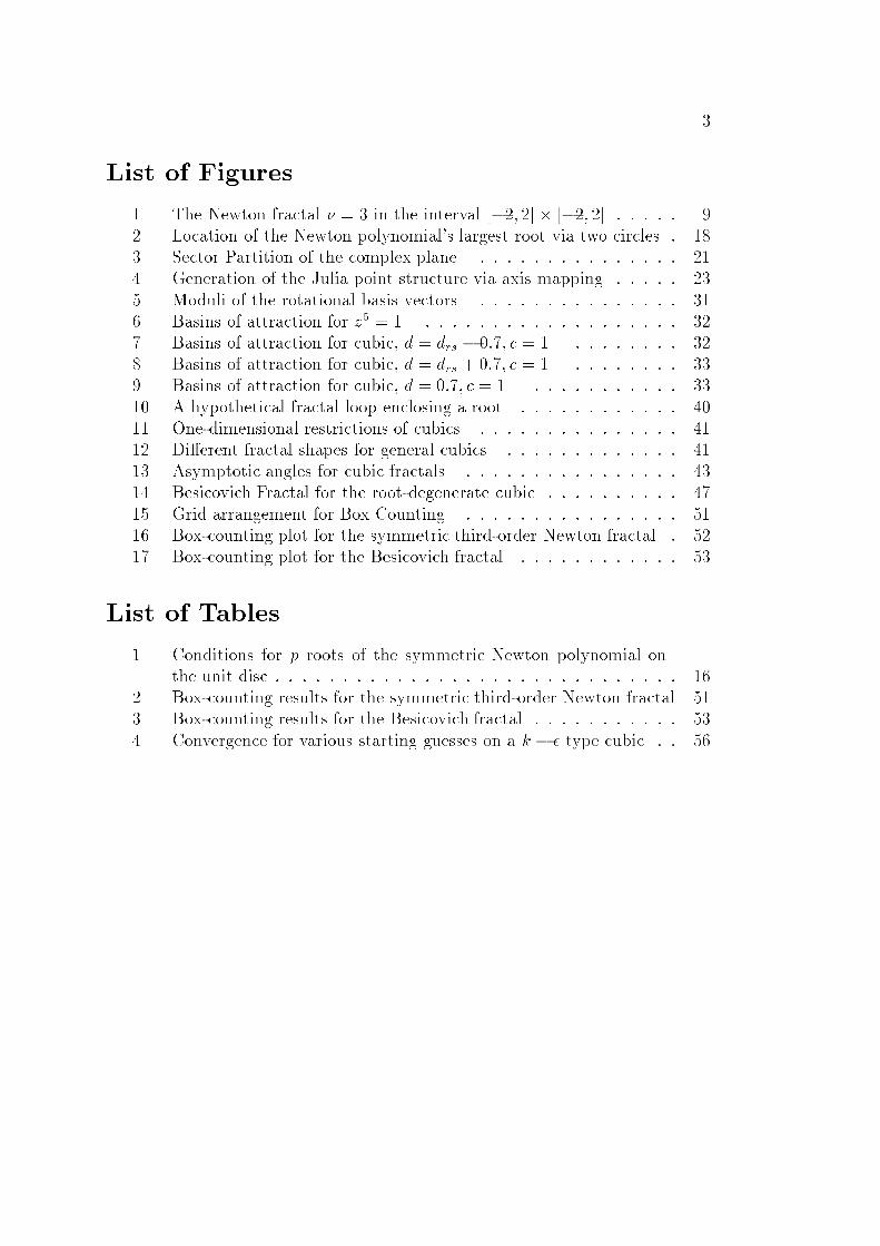
3List of Figures1 The Newton fractal � = 3 in the interval [�2; 2]� [�2; 2] : : : : : 92 Location of the Newton polynomial's largest root via two circles : 183 Sector Partition of the complex plane : : : : : : : : : : : : : : : 214 Generation of the Julia point structure via axis mapping : : : : : 235 Moduli of the rotational basis vectors : : : : : : : : : : : : : : : 316 Basins of attraction for z5 = 1. : : : : : : : : : : : : : : : : : : : 327 Basins of attraction for cubic, d = drs � 0:7; c = 1. : : : : : : : : 328 Basins of attraction for cubic, d = drs + 0:7; c = 1. : : : : : : : : 339 Basins of attraction for cubic, d = 0:7; c = 1. : : : : : : : : : : : 3310 A hypothetical fractal loop enclosing a root : : : : : : : : : : : : 4011 One-dimensional restrictions of cubics : : : : : : : : : : : : : : : 4112 Di�erent fractal shapes for general cubics : : : : : : : : : : : : : 4113 Asymptotic angles for cubic fractals : : : : : : : : : : : : : : : : 4314 Besicovich Fractal for the root-degenerate cubic : : : : : : : : : : 4715 Grid arrangement for Box Counting : : : : : : : : : : : : : : : : 5116 Box-counting plot for the symmetric third-order Newton fractal : 5217 Box-counting plot for the Besicovich fractal : : : : : : : : : : : : 53List of Tables1 Conditions for p roots of the symmetric Newton polynomial onthe unit disc : : : : : : : : : : : : : : : : : : : : : : : : : : : : : : 162 Box-counting results for the symmetric third-order Newton fractal 513 Box-counting results for the Besicovich fractal : : : : : : : : : : : 534 Convergence for various starting guesses on a k � � type cubic : : 56

4Description of the Colour PlatesFig. 6 Basins of attraction for z5 = 1, using the orthodox Newton method. Arrayof 300 � 300 equidistant points cast over [�1:5; 1:5]� [�1:5; 1:5]. An o�set of k � 50has been added to the actual iteration number according to the converged solution.Colouring according to converged solution� blue for root (1; 0), iteration range 1 . . .45,� green for root e 2�5 , iteration range 50 . . .95,� orange for root e 4�5 , iteration range 100 . . .145,� yellow for root e 6�5 , iteration range 150 . . .195,� red-brown for root e 8�5 , iteration range 200 . . .245.Fig. 7 Basins of attraction for z3+ dz� c = 0, using the orthodox Newton method.Coe�cients d = � � 33p4 + 0:7� ; c = 1. Array of 240� 240 equidistant points cast over[�2; 2] � [�2; 2]. An o�set of k � 85 has been added to the actual iteration numberaccording to the converged solution. Colouring according to converged solution� blue for positive root, iteration range 1 . . .80,� yellow for large negative root, iteration range 85 . . .160,� green/red for small negative root, iteration range 170 . . .250.Fig. 8 Basins of attraction for z3+ dz� c = 0, using the orthodox Newton method.Coe�cients d = � � 33p4 � 0:7� ; c = 1. Array of 240� 240 equidistant points cast over[�2; 2] � [�2; 2]. An o�set of k � 85 has been added to the actual iteration numberaccording to the converged solution. Colouring according to converged solution� blue for positive real root, iteration range 1 . . .80,� green/red for negative root with =(z) > 0, iteration range 85 . . .160,� yellow for negative root with =(z) < 0, iteration range 170 . . .250.Fig. 9 Basins of attraction for z3+ dz� c = 0, using the orthodox Newton method.Coe�cients d = 0:7; c = 1. Array of 240 � 240 equidistant points cast over [�2; 2]�[�2; 2]. An o�set of k � 85 has been added to the actual iteration number according tothe converged solution. Colouring according to converged solution� blue for positive real root, iteration range 1 . . .80,� green/red for negative root with =(z) > 0, iteration range 85 . . .160,� yellow for negative root with =(z) < 0, iteration range 170 . . .250.

51 IntroductionDespite being a widely used algorithm to solve non-linear systems, little is knownabout the global behaviour of Newton's method. Practitioners usually rely on thelocal Newton-Kantorovich convergence result [21] and employ Newton's methodas a local solver depending on some suitably chosen residual. If the residual doesnot decrease as speci�ed, a globally more stable method is used to �nd a betterstarting estimate for the solution. Some strategies of this kind can be foundin [16], [19]. Another approach is to stabilise Newton's method by operationson the variable shifts ([5], [8], [12]). Such a method might be stable for someapplications, but good convergence is not guaranteed due to the existence of localminima that can slow convergence down.One aspect of a globally applied Newton method is that the basins of attrac-tion for di�erent roots of a non-linear problem might have fractal boundaries.In addition to possible singularities of the problem, this introduces orbits intothe convergence history that can slow convergence down considerably. As thefractal structure has not been completely understood, this is used as an indi-cator that Newton's method has globally unpredictable behaviour. However, ithas been shown in [6] for the complex cubic that the convergence behaviour ofNewton's method can be explained once the underlying fractal problem has beenunderstood.Historically, the problem of applying Newton's method to complex polynomi-als has been �rst addressed by Schroeder in 1871. Given a quadratic z2 � 1, heasked to which of the two roots an arbitrary starting point in the complex planewould converge. The solution to this question on the boundary of the basinsof attraction was the imaginary axis, found immediately by himself. In 1879,Cayley asked the same question for a symmetric cubic z3 � 1, not being ableto give an answer. The question became known as Cayley's problem. In a sub-stantial paper, Gaston Julia ([11]) used this problem as an example of describingsets that later came to bear his name. The Julia set may be described as theunion of all points that are eventually mapped onto a singular point. An exactde�nition is given later. Julia also derived some properties of the set solvingCayley's problem, namely a re ective symmetry with respect to the real axis,and invariance under rotations by multiples of 2�3 and the inclusion of z = 0and z = 1 as images of each other. Also, the fragmented character of the setwas mentioned in the sense that it could not immediately described by Jordancurves. However, a comprehensive solution to Cayley's problem was not given.Almost seven decades later, interest in iterated polynomial mappings and theirproperties re-emerged, but much attention was devoted to the Mandelbrot set([2], [13], [17]) and Newton's method was only treated in a historical contextand as an accessible example to introduce the concept of Julia sets [18]. Forthe numerical use of Newton's method, some e�orts were made to bound thenumber of iterations needed for convergence from any starting point ([14], [20])

6and to show convergence in a statistical sense. However, a comprehensive solu-tion to Cayley's problem still was not available. The aforementioned researchfocused on the general properties of Julia sets rather than on speci�c propertiesof Newton's method. By changing this approach and examining the mechanismby which Newton's method generates a fractal structure, a �rst comprehensivesolution to Cayley's problem was given in [6], deriving all characteristic scale fac-tors and symmetries, and uniting these results to give a fractal dimension of thestructure. In addition, an approximation to the fractal structure was given thatconsists only of Jordan curves and thus can be computed without the extensiveuse of computer graphics.This work will continue on the lines set out in [6]. It will generalise theresults of the symmetric cubic z3�1 to the general symmetric polynomial z��1.The fractal structure will be explained from �rst principles and a quantitativedescription will be stated as far as analytic solutions permit this. Two di�erentapproaches will be taken for the generation of the fractal structure, both leadingto the same result. One approach relies on the classical root analysis, whereasthe other uses a rotational representation of the solutions to polynomials similarto the one presented in [6]. The rotational approach to us seems more intuitiveand generalisable to other problems. We will also state a way to approximatethe fractal structure by Jordan curves. The quantitative results stated includeboth local and global symmetries, scale factors and a general way to estimatethe fractal dimension of the structure.In the second part, we will restrict the analysis to general polynomial prob-lems of degree 3. A general 'fractal map' is established, showing how the appear-ance of the fractal varies with the parameters of the cubic. Again, characteristicproperties are stated quantitatively. Special cases are examined and are shown tobe transitionary states between the three general fractal types that are possiblefor general cubics. The symmetric cubic is one of these cases. Another case isshown to yield a fractal of Besicovich type, that has so far not been associatedwith Newton's method. The fractal dimension for this fractal is computed us-ing the previously established theory for the generation of polynomial Newtonfractals.The third part will verify the theoretical results on the fractal dimension usingan experimental box-counting approach and show how the results on generalcubic fractals can be applied directly to a problem in turbulence modelling. Itwill be shown that for this problem, no stabilisations of Newton's method arenecessary if the starting point is chosen in accordance with the fractal results.These results, however, contradict the physical intuition that is commonly usedto �nd a starting approximation. The superior numerical behaviour of such acounter-intuitive guess is demonstrated in experiments.The work concludes with a brief summary of the results. We will also discussthe numerical relevance of the theoretical results on the fractal structure.

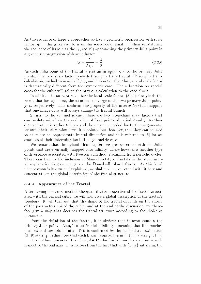
72 The Symmetric Newton Fractal of Order �As mentioned above, it is well established that the boundaries of the basins ofattraction for di�erent roots of certain polynomials are fractals. We will �rstgive the necessary de�nitions for a technical discussion. For a certain class ofpolynomials, properties for the associated fractals will be stated in a quantitativefashion. For a detailed derivation and an example of the signi�cance of theseproperties in the case of a cubic polynomial, we refer to [6]. We will then presenta general construction principle for the fractal structure that has not appearedin the literature and can be used to explain most of the fractal features.2.1 De�nitionsThis section will be discussing a special class of polynomials de�ned in the fol-lowing fashion.De�nition 2.1 The symmetric polynomial of order � is de�ned byz� = 1; z 2 C; � 2 N; � > 2: (2.1)We will examine the basins of attraction for the roots of these symmetric polyno-mials when Newton's method is used as a numerical procedure for root-�nding.Throughout this report, we will be concerned with Newton's method de�ned inthe standard way.De�nition 2.2 The orthodox Newton method on f(z) is de�ned by the iterationz(k+1) = z(k) � f(z(k))fz(z(k)) = g �z(k)� (2.2)with z(k) denoting the kth iterate, and fz denoting dfdz .It is noted from the de�nition that the roots zk of f(z) with f(zk) = 0 are stable�xed points of the Newton iteration.The view we shall take of the Newton method is slightly di�erent to thatimplied by (2.2). Rather than �nding the next iterate given a starting point,we shall ask which points z(k) = z are mapped into a given point z(k+1) = z0 by(2.2). We therefore de�neDe�nition 2.3 The complex Newton polynomial of order � is de�ned by(� � 1)z� � �z0z��1 + 1 = 0; z; z0 2 C (2.3)Despite the existence of a 'common-sense concept' of a fractal, it can bedi�cult to give a general de�nition for such a structure. Following Mandelbrot[13], a strict de�nition of a fractal is

8De�nition 2.4 A fractal is a set for which the Hausdor�-Besicovitch dimensionstrictly exceeds the topological dimension.This de�nition, however precise, is hard to apply in practice if the Hausdor�-Besicovitch dimension is di�cult to determine or even unknown - which in fact isthe case for many well-known fractals. Therefore, alternative and more intuitivede�nitions of a fractal are in use. For the purposes of this study, we use 'fractal'according to the de�nition by Falconer [7].De�nition 2.5 We refer to a set S as a fractal with the following in mind.� S has a �ne structure, i.e. detail on arbitrary small scales.� S is too irregular to be described in traditional geometrical language, bothlocally and globally.� Often S has some form of self-similarity, perhaps approximate or statistical.� Usually, the 'fractal dimension' of S (de�ned in some way) is greater thanits topological dimension.� In most cases of interest S is de�ned in a very simple way, perhaps recur-sively.A suitable working de�nition for the purposes of this study isDe�nition 2.6 The Newton fractal of order � is de�ned by the union of allpoints that are mapped into the singular origin by the Newton mapping (2.3).It is obvious from this de�nition that with z belonging to the Newton fractal,z0 also belongs to the fractal. A picture of the Newton fractal in the vicinity ofthe origin can be seen in Fig. 1. It is worth noting that the fractal is the union ofpoints that lie on the boundary of the basins of attraction, and does not consistof the basins themselves. Fig. 5 also provides a good illustration for most of thepoints in de�nition 2.5.As this study is concerned with the iteration of a function of a complexvariable, we will refer to the underlying framework of Julia set theory. FollowingFalconer [7], we de�ne the necessary sets as follows.De�nition 2.7 The Julia set J (g) of a complex-variable function g is the clo-sure of the set of repelling periodic points of g.De�nition 2.8 The Fatou set F(g) of a complex-variable function g is the com-plement of the Julia set J (g). F(g) is also known as the stable set of g.Using this, we could equivalently de�ne the Newton fractal as the union of allJulia points of the Newton mapping. An important notion for identifying Juliapoints on the fractal structure will be their order.

9-2.0 -1.5 -1.0 -0.5 0.0 0.5 1.0 1.5 2.0

-2.0

-1.5

-1.0

-0.5

0.0

0.5

1.0

1.5

2.0

Figure 1: The Newton fractal � = 3 in the interval [�2; 2]� [�2; 2]De�nition 2.9 The order of a speci�c Julia point on a Newton fractal is de�nedas the number of Newton iterations it takes to reach the origin from that point.An excellent overview of the Julia set theory concerned with polynomials ofa complex variable can be found in Falconer's book [7]. In this work, we want tohighlight one particular theorem that is very instructive for understanding thecharacter of fractals associated with polynomials and Newton's method. We �rsthave to de�ne the important concept of a basin of attraction.De�nition 2.10 The basin of attraction A(w) of an attractive �xed point w ofa function g is de�ned by A(w) = fz 2 C : gk(z)! w as k !1 g.With this de�nition, we are able to state the theorem.Theorem 2.11 Let w be an attractive �xed point of g. Then, denoting theboundary of the basin of attraction A(w) by @A(w), we get: J (g) = @A(w). Thesame is true if w =1.For a proof and further background on Julia set theory, see [7]. One implica-tion of the theorem is that any point of the Julia set must lie on the boundary ofall basins of attraction for all attractive �xed points of g. Thus, an approximateclose to a Julia point with only a small perturbation might converge to any ofthe roots. Further aspects of this theorem will be discussed in later sections. Acolour plot of the basins of attraction for a polynomial of degree 5 illustratingthe fractal character and theorem 2.11 is given in Fig. 6.

102.2 General PropertiesAfter having prepared the ground, we can now present a more technical analysisof the general inverse mapping (2.3) and the emerging Newton fractal. Thenecessary results are derived brie y, referring to [6] for a more detailed discussionand the example � = 3.Classical Results It follows directly from (2.1) that the roots associated withthe vth-order symmetric polynomial arezk = e 2�� (k�1)i; k = 1; 2; . . . ; �: (2.4)The primary Julia point that is caused by a singularity of the derivative in (2.2)is always �0 = 0: (2.5)Parent Structure It can be easily obtained from (2.3) that the �rst-orderJulia points which arise from applying the inverse Newton iteration to the originonce are �1;k = 1�p� � 1 � e�� (2k�1)i; k = 1; 2; . . . ; �: (2.6)Therefore, their distance from the origin for the �th order Newton fractal isr = 1�p� � 1 ; (2.7)approaching 1 for large �. Comparing (2.4) and (2.6), it can be seen that the�rst-order Julia points always lie between two neighbouring roots.As we shall see later, these points de�ne the parent structure that contains thewhole information needed to describe the fractal. The concept of the attractivecircle that was a very useful approximation for � = 3 cannot be extended forgeneral �, as the parent structure contains points with a greater radius than r.However, all the concepts associated with the attractive circle generalise.Global Symmetry By inspection, it can be established that (2.3) is invariantunder the coordinate transformationz 7! ze 2�m� i; z0 7! z0e 2�m� i m 2 N: (2.8)This is equivalent to subsequent rotations by 2�� with the origin as a centre.Furthermore, we can see that (2.3) is invariant toz 7! z�; z0 7! (z0)�; (2.9)

11with z� denoting the conjugate of z. The combination of rotational and re ectivesymmetry dictates that the branches of the fractal lie on straight lines.Therefore, the Newton fractal of order � has a �-fold global rotational symme-try and hence consists of � branches. It also has a re ective symmetry regardingthe real axis. The � branches lie along straight lines.Global Scale Factor For large z; z0 (jzj; jz0j � 1), the governing equation(2.3) can be expanded as z0 = � � 1� z +O �z1��� : (2.10)As both z and z0 are contained in the fractal, the fractal is invariant under thescaling z 7! ��;1z; ��;1 = �� � 1 : (2.11)It has to be noted that this exact invariance is only achieved in the limit jzj ! 1.As an approximation, it may however be used much earlier. We therefore statethat the Newton fractal of order � has a global scale factor of ��;1.Local Symmetry Following the result on global symmetry, we de�ne theglobal symmetry axes Ls to be the lines through the origin and the �rst-orderJulia points as de�ned in (2.6). We parametrise the axes byz0 = �ei�s; �s = �� + 2�� s; 0 � � <1: (2.12)Approximating the solution to (2.3) for large z0 byz = 1��1p�z0 +O z� 2��1(��1)20 ! ; (2.13)we obtain for the sth global symmetry axis and � � 1zsm(�) � 1��1qj��j � e i��1 �s � e 2�i��1m; m = 0; 1; . . . ; (� � 2): (2.14)Again, the zsm asymptotically approach the origin on straight lines for large �.The succession of Julia points on these lines will be discussed in relation withlocal scale factors. The angle !sm, from which the zsm approach the origin, canimmediately be written as!sm = ��(� � 1) [1 + 2(m� + s)] : (2.15)

12By inspection, (m� + s) ranges from 0 to �(� � 1)� 1, and therefore the anglesare !k = ��(� � 1) + 2��(� � 1)k; k = 0; 1; . . . ; �(� � 1)� 1: (2.16)It can be seen that the angles !k = 0 and !k = � never occur. The interpretationof this formula is that �(� � 1) locally identical branches of the fractal approachthe origin with an angle of �� = 2��(� � 1) (2.17)between neighbouring branches. An example of this discussion for � = 3 is givenin section 3.4.1 of [6].We see that the local symmetry is an integer multiple of the global symmetry.This property is characteristic for all Newton fractals. We note that, as eachJulia point is a locally conformal image of the origin, the local symmetry holdsthroughout the fractal. We can summarize that the Newton fractal of order �is locally invariant to rotations by �� and exhibits �(� � 1)-fold local rotationalsymmetry at each point.Local Scale Factors We note that (2.13) yields small z for large z0 and there-fore is suitable for approximating the local behaviour at the origin. Consideringthe geometric progressionz0; ��;1z0; (��;1)2 z0; . . . (2.18)that describes Julia points for a suitable starting point jz0j � 1, the progressionmapped close to the origin by (2.13) is1��1p�z0 ; 1��1q��;1�z0 ; 1��1q(��;1)2 �z0 ; . . . : (2.19)This again is a geometric progression; the scale factor can be determined as�� = ��1s� � 1� = ��1q(��;1)�1: (2.20)We see that �� is rapidly approaching 1 as � grows -�� = �1 � 1�� 1��1 � 1 � 1�(� � 1) : (2.21)The geometrical interpretation of this result is that the Julia points on a chain oforder n (obtained from the negative real axis after n inverse Newton mappings)

13approach the Julia point of order (n�1) in a geometrical progression with factor�� . This holds particularly for the straight lines approaching the origin that weredescribed in the preceding paragraph. As � is growing, the Julia points on thatbranch are more equally spaced and, as there is an in�nite number of them oneach branch, they appear more densely crowded.Following an argument in [6] and using the previously established properties,we can state that the parent structure of the fractal will be a blob bordered bytwo fractal chains and a number of chains running inside, the total number ofchains per blob being (� � 1) due to the results on symmetry. Aside from eachchain having a scale factor �� along itself, there exist scale factors that determinethe local scaling when a point changes from one branch to the other in a Newtonstep, the so-called cross-chain scale factors ��;k.It is not possible to state general expressions for all cross-chain scale fac-tors involved. According to [6], we can give an expression for the scale factorsassociated with �xed points of cycle ���;2;k = 12(� � 1) sin �k� ; k = 1; 2; . . . ; � � 1: (2.22)Although not being able to state them explicitly, we can give an argumentfor the number of di�erent cross-chain scale factors that should occur. It can benoted that the blobs of the �th order Newton-fractal consist of (� � 1) brancheswhich are arranged symmetrical around the centre line of the blob. If � is even,the centre line coincides with one of the branches. Furthermore, the blobs oneach branch (which are relevant for the next step of the inverse mapping) arecomposed of (� � 1) sub-branches. This leads to a total number of (� � 1)2 sub-branches. We now take the symmetrywith respect to the centre line into account,in particular the fact that for even �, one (the centre) branch is symmetrical initself. This reduces the number of di�erent sub-branches tob� = b12 h(� � 1)2 + 1ic; (2.23)with each of which a cross-chain scale factor should be associated. b�c denotesthe integer truncation operator (e.g. b2:8c = 2).Again, due to the local conformity of the inverse Newton mapping, we cangeneralise these results for the origin for all points of the fractal. The Julia pointsof order n approach the point of order (n� 1) on a branch with local scale factor�� as a geometrical progression. There are b12(� � 1)c di�erent cross-chain scalefactors ��;2;k for cycle � and b� di�erent cross-chain scale factors in general.Fractal Dimension Following an argument presented in [6], we state an ap-proximation to the fractal dimension of the �th-order Newton fractal involvingall the di�erent scale factors. If the fractal dimension is d, it must satisfy the

14following equation b�Xk=1 (��;k)d + �d� = 1: (2.24)This equation was derived on the assumption of geometric progressionsthroughout the fractal chains and therefore only is an approximation to thereal fractal structure. However, we consider it a rather useful and elegant one.Comparisons of the obtained fractal dimensions with box-counting experimentswill be presented in the section on numerical experiments. The equation corre-sponds to the one stated in [2] for hyperbolic systems of iterated functions andderived independently there. It gives the Hausdor�-Besicovich dimension for theattractor of disconnected or just-touching systems, a class to which the Newtonfractals belong.2.3 Structural Results from Classical Root AnalysisBeing a polynomial of degree � with complex coe�cients, the Newton polynomialcan be subjected to an analysis concerning the location of its roots. This will giveresults on the fractal structure and can explain the appearance of the symmetricNewton fractal of order �. We start by establishing bounds on the moduli of theroots and then determine approximations for their arguments. As most of thetheorems used to determine the results are well established in complex analysis,we refer to the literature for proofs and the general statement of the theorems.Without loss of generality, it is assumed that the roots can be ordered accordingto their modulus as jz1j � jz2j � . . . � jz�j: (2.25)When quoting a theorem from the literature, we will assume that the polynomialis written in the form p(z) = �Xk=0 akzk (2.26)with coe�cients ak 2 C, unless otherwise stated.Bounds for the root of largest modulus Di�erentiating (2.3) with respectto z, we obtain fz(z) = �(� � 1)z��2 (z � z0) : (2.27)This derivative has roots atf�1 = z0g _ f�k = 0g; k = 2; . . . ; � � 1: (2.28)

15Knowing the location of the roots of the derivative fz(z), the Gauss-Lucas the-orem (Theorem 6.5a, [10]) states that they must lie in the convex hull of the setof zeros of the polynomial f(z). Therefore, for the given geometry of derivativeroots, at least one zero of the Newton polynomial must have modulus larger thanjz0j (and be located in roughly the same direction in the complex plane as z0).Furthermore, for a polynomial of the form (2.26), the zero of largest moduluscan be bound by (Theorem (27,3), [15])� � jz1j � ��p2�1 ;� = max1�k�� ����� a��ka�C(�; k) ����� 1k (2.29)with C(�; k) = �!k!(��k)! denoting the binomial coe�cient. Substituting the coe�-cients ak of the Newton polynomial, it is obtained for �� = max jz0j� � 1 ; 1�p� � 1! : (2.30)The �rst bound in the maximum operator can be discarded in favour of thesharper bound obtained from the above argument using the Gauss-Lucas theo-rem.We can therefore state the followingLemma 2.12 The zero of largest modulus z1 of the Newton polynomial (2.3) canbe bounded from below byjz1j � max jz0j; 1�p� � 1! : (2.31)For a more convenient upper bound, we examineg(z) = �p2� 1 � 1� (2.32)to �nd it has a root at � = 1 and a local minimum with g(z) < 0 wheregz(z) = 1�2 � �p2 ln 2� 1� = 0: (2.33)Zero is approached from below as � !1. Hence, we can state for the region ofinterest � > 2 �p2� 1 < 1� (2.34)and therefore establish

16Lemma 2.13 The zero of largest modulus z1 of the Newton polynomial (2.3) canbe bounded from above byjz1j � 1�p2� 1 max jz0j� � 1 ; 1�p� � 1! (2.35)For large � and jz0j, this bound approachesjz1j � �� � 1 jz0j: (2.36)Bounds for the remaining (� � 1) roots Following a result by Cohn ([15],p.130), a polynomial of the form (2.26) has exactly p zeros on the unit disc, ifjapj > �Xk=0 jakj(1� �kp): (2.37)The various possibilities for p substituting the coe�cients of the Newton poly-nomial (2.3) are given in Table 1.p japj P jakj(1� �kp) condition for jzpj � 1� � � 1 �jz0j+ 1 jz0j < ��2�� � 1 �jz0j � jz0j > 11 < p < � � 1 0 � + �jz0j not possible1 1 � � 1 + �jz0j not possibleTable 1: Conditions for p roots of the symmetric Newton polynomial on the unitdiscFrom this table, we can concludeLemma 2.14 Of the � roots of the Newton polynomial (2.3), the unit disc jzj � 1contains� all � roots for jz0j < ��2� ,� exactly (� � 1) roots for jz0j > 1.Using a generalisation of Cauchy's theorem on a disc containing a given num-ber of roots by Van Vleck (Theorem 6.4n, [10]), we obtain

17Lemma 2.15 The disc de�ned byjzj < 1��1qjz0j (2.38)contains at least (��1) roots of the Newton polynomial (2.3). It contains exactly(� � 1) roots for jz0j > 1, according to lemma 2.12.Regarding lower bounds for the roots, we can expand the polynomial at z = 0,and obtain (Theorem 6.4b, [10]) for the radius of a circle that contains no roots� = 12 � min1�m�� ���� a0am ���� 1m : (2.39)Substituting the coe�cients of the Newton polynomial, we can stateLemma 2.16 The � roots of the Newton polynomial (2.3) are bounded frombelow by jzkj > 12 min0@ 1�p� � 1 ; 1��1q�jz0j1A k = 1; 2; . . . ; � (2.40)Estimates for the Argument of the Largest Root Parametrising the New-ton polynomial along the fractal's global symmetry axes and rotating the struc-ture accordingly,z0 = �e (2k�1)�� i; z = �e (2k�1)�� i; k = 0; 1; . . . ; � � 1; (2.41)a polynomial with real coe�cients(� � 1)�� � �����1 + 1 = 0 (2.42)is obtained. As, parametrising � = ��; � 2 R1 + ���� �� � 1� ��� (2.43)changes sign for � > 1, there exists a real root z1 with jz1j > jz0j and an argumentidentical to that of z0. We therefore haveLemma 2.17 For z0 being a Julia point on one of the fractal's global symmetryaxes, arg(z1) = arg(z0): (2.44)

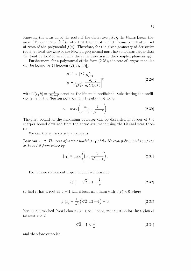
18For later discussion, it is also noted that with the coe�cients in (2.42) being real,all roots must be in conjugate complex pairs.Recalling the de�nition of Newton's method (2.2), the Newton polynomialcan also be stated asp(z)� z0� � 1pz(z) = 0; p(z) = z� + 1� � 1 : (2.45)In this form, a result by Walsh and Marden (Corollary (18,1), [15]) can be em-ployed directly, stating that the roots of (2.45) must be located within the discthat contains the roots for p(z) and its translation by z0��1 . We therefore obtainLemma 2.18 The roots of the symmetric Newton polynomial (2.3) lie in theunion of the discs with radius � and center ck, where� = 1�p� � 1 ; c1 = 0; c2 = �� � 1z0: (2.46)x

y

z0

c2

x

y

z0 c2Figure 2: Location of the Newton polynomial's largest root via two circlesKnowing from lemma 2.12 that the root of largest modulus must lie in thecircle with centre c2, we can use a geometrical argument on the intersection ofthe two circles with radius � and displacement jc2j and obtainLemma 2.19 The argument of z1, the root of largest modulus of the symmetricNewton polynomial can be bounded from above byarg(z1) � arg(z0)� arccos jc2j2� ; jc2j � p2� (2.47a)arg(z1) � arg(z0)� arccos qjc2j2 � �2jc2j ; jc2j � p2�: (2.47b)

19It can be seen that for large jz0j, the argument of z1 approaches that of z0.To further improve the bound on the argument for small z0, we state thefollowingLemma 2.20 The lines through the origin and the roots of the symmetric poly-nomial (2.1) z = �e 2k�� i; � > 0; k = 0; 1; . . . ; � � 1 (2.48)contain no Julia points.We note that this lemma can be used for an elegant proof of theorem 2.11, takinginto account that every point of the fractal is a locally conformal image of theorigin and the origin connects to each root in a straight line that contains noJulia points.Proof Without loss of generality, we restrict the proof to the case k = 0, thepositive real axis. The proof will then hold for all the other lines due to the rotationalsymmetry of the structure. We consider the Newton iteration (2.2) on the real axisa = � � �� � 1����1 = (� � 1)�� + 1����1 : (2.49)As a > 0 for � > 0, the positive real axis is mapped onto itself under the Newtoniteration. Furthermore, d2dz2 f = �(� � 1)���2 (2.50)for the symmetric polynomial of order �, every point on the positive real axis convergesinto the root � = 1 due to convexity. As the positive real axis is mapped onto itselfand contains only convergent points, it must be fully contained in the Fatou set andtherefore cannot contain any Julia points. 2This result will be needed again when establishing bounds on the remainingroots of the Newton polynomial as the lines through the roots of the symmetricpolynomial constitute a separatrix of the fractal. For the root of largest modulus,it helps establishingLemma 2.21 The argument of the largest root of the symmetric Newton poly-nomial cannot exceed the upper boundarg(z1) � arg(z0)� �� : (2.51)As the modulus of z1 is bounded from below by lemma 2.12, the above boundson the argument con�rm the 'prolongation in the direction of z0'.

20Bounds on the argument of the (� � 1) remaining roots To estimatethe location of the remaining roots of the symmetric polynomial, we have toconsider the location of the coe�cients of (2.3) in the complex plane. We noticethat a� and a0 both are positive real, and only a��1 has a variable location,solely determined by z0. Using this information, we can state the importantresult (Theorem (41,3), [15])Lemma 2.22 If = arg(z0), then the sector in the positive real half-plane de-�ned by arg(z) < 1� (� � 2 ) (2.52)contains � roots of the symmetric Newton polynomial with� � = 0, if <(z0) < 0.� � � 2, if <(z0) > 0.Proof The coe�cients of the symmetric Newton polynomial are, ordered by theirindices, a� = (� � 1); a��1 = ��z0; a0 = 1: (2.53)Therefore, the double sector de�ned by j arg(z0) � �j contains all coe�cients. If<(z0) < 0, all coe�cients lie in the same sector, whereas for <(z0) > 0, the sequenceof coe�cients changes sector twice. According to Theorem (41,3), [15] this de�nes themaximal number of roots in the stated positive sector. 2Considering the rotational symmetry of the fractal, we now divide the com-plex plane into � sectors with angle 2�� centered at the origin by drawing linesconnecting the origin with the �rst-order Julia points �1;k. Recalling the localconformity of the inverse Newton mapping, we know that for small z0, the New-ton polynomial has a simple root close to each of the � points �1;k. Furthermore,lemma 2.20 states that for points on the fractal, the bisectors of the � sectorsde�ned by the �1;k cannot be crossed. Therefore, for small z0, the � roots arecon�ned to the � global branches of the fractal. However, as the roots of apolynomial vary smoothly with changes in the coe�cients according to Rouch�e'stheorem (Theorem 4.10c, [10]) and the fractal is a dense structure by theorem2.11, they will be con�ned to the vicinity of the global symmetry axes for all z0on the fractal. From lemma 2.17, we can conlude that there must be an approxi-mate conjugacy of the roots with respect to the symmetry axis closest to z0. Wecan therefore concludeLemma 2.23 The � roots of the Newton polynomial (2.3) are located close tothe global symmetry axes of the fractal, if z0 is a Julia point. The (��1) axes notpointing in the general direction of z0 each have a simple root in their vicinity.The roots obey an approximate conjugacy with respect to the symmetry axis closeto z0, depending on the deviation angle of z0 from that axis.

21Lemma 2.22 can be used to establish further bounds on how close the rootslie to the symmetry axes regarding their position to z0. As these are only oftechnical interest, we will not pursue this further.Structural Conclusion We have now established the necessary framework fora description of the fractal structure from �rst principles.To do so, we partition the complex plane into � sectors centered at the originthat open with an angle of 2�� and are bisected by the rays Ls connecting theorigin with the �rst-order Julia points �1;k. It is immediately clear from (2.4) thatthe roots of the polynomial (2.1) de�ne the borderlines between these sectors.Fig. 3 shows such a partition for the case � = 5.x

y

root

first-order Julia pointFigure 3: Sector Partition of the complex planeFurthermore, as stated earlier, we denote that part of the fractal that connectsthe origin and the �rst-order Julia points �1;k as the parent structure. We denotethe structure connecting two Julia points of ascending order on the bisecting axisLs of a sector as a blob structure. We are now able to stateTheorem 2.24 For any Julia point �k, there exist � images under the inverseNewton mapping de�ned by (2.3) with the following properties:� One solution is located in the same sector as �k, prolongated along thebisecting axis of that sector by one blob structure.� (� � 1) solutions are located on the parent structure in the (� � 1) sectorsthat do not contain �k, each sector containing one solution. The parentstructure is contained within the unit disc.Proof We �rst comment on the preliminary de�nitions and statements. It isimmediately obvious from (2.3) that the � �rst-order Julia points exist as stated. Bythe local conformity property of the inverse Newton mapping, both the origin andthe �1;k must be locally of similar structure. Due to theorem 2.11, there has to exist

22a dense fractal structure connecting these two points, the parent structure. Due tolemma 2.17, the �rst-order Julia points are the beginning of a chain of Julia pointson the bisecting axis in each sector. As the fractal structure approaches the origin instraight lines at equal angles (see the earlier results on local symmetry), it approacheseach of these points in the same fashion, thereby de�ning "knots" on the bisecting axisLs. The structure connecting two of these knots must by theorem 2.11 be dense, hencefollows the existence of the blob structure.The �rst assertion of theorem 2.24 is proven by combining lemma 2.12 and 2.13 forthe modulus, and lemma 2.17, 2.19, 2.21 for the argument of the largest root. Lemma2.18 gives a geometrically suggestive result on the prolongation along the bisectingaxis, which coincides with the general direction of �k for Julia points.The second assertion is proven by lemma 2.14 and 2.15 for the modulus, and lemma2.23 for the argument of the solutions. Lemma 2.14 de�nes the upper bound on thesize of the parent structure. The images of �k can be bounded from below using lemma2.16. 2Theorem 2.24 has stated properties of the pointwise mapping of Julia points.Combined with the other results on the inverse Newton mapping, we can use itto state a theorem giving a description of the fractal structure via Jordan curves.Theorem 2.25 The fractal structure can be approximated by successive inverseNewton mappings of the bisecting axes of the � sectors de�ning the fractal, eachcontaining an in�nite number of Julia points. In the limit of in�nitely manyinverse mappings of that structure, the Newton fractal of order � is obtained.An example of the theorem for the case � = 3 is given in [6].Proof The existence of in�nitely many Julia points on each bisecting axis can beconcluded from lemma 2.17, with the primary Julia points �1;k starting the recursionon the axis. The same lemma ascertains that one image of any point on the axis willlie on the same axis (and its extension through the origin), this structure constitutingan invariant of the mapping. Due to local conformity of the inverse Newton mapping,the image of the axis (which is obviously a Jordan curve) will also be a Jordan curve.As the origin �0 is mapped onto in�nity and �1;k onto the origin by one Newton step,the part of the axis connecting (0; 0) and �1;k extending to in�nity must have (� � 1)images connecting the �1;k and the origin �0. These lie, according to theorem 2.24, onthe parent structure of the fractal.By the de�nition of the inverse Newton mapping, every curve that connects twoJulia points of order (k�1) and k will be mapped onto a line that connects Julia pointsof order k and (k+1) by that mapping and the order of any Julia point on that line willalso be increased by one. On the other hand, the order of all Julia points on a curvewill be decreased by one when the curve is subjected to one Newton step. However,all Julia points on the fractal will eventually be mapped onto one of the bisecting axesLs - namely onto �1;k - when subjected to consecutive Newton steps. As every inverseof the Ls also maps the �rst-order Julia points contained on them and every Juliapoint is an image of �1k , the whole fractal can eventually be obtained by subjectingthe bisecting axes Ls to the inverse Newton mapping. 2

2321 3

2-1 2-22-3 3-2 3-33-1

(0)

(1)

(2)

(3)Figure 4: Generation of the Julia point structure via axis mappingFig. 4 illustrates the generation of the fractal structure via consecutive axismappings for the case � = 3. We consider the thick line on the left of the treeto be the initial axis. It has, according to theorem 2.24, a prolongated solutionand two images in the other sectors. Geometrically, these images connect the�1;k with the origin �0 via a sequence of in�nitely many Julia points, depictedby the thick dashed lines. The two images 2 and 3 again have images obeyingtheorem 2.24, each connecting a Julia point of order 2 with one of order 1 viain�nity. The in�nite chain of Julia points is depicted by a thin dashed line, andthe straight line denotes the connection between start and end point of the chain.It is important to note that the dependencies between Julia points in Fig. 4 donot correlate with the dependencies dictated by the inverse Newton mapping, i.e.the three second-order Julia points in the tree are not direct images of the onedirectly above. The images of the axes could not be depicted straightforwardlyon a tree that displays the mapping dependencies. However, the nodes of such atree and the tree depicted in Fig. 4 are identical. All the remaining branches ofthe tree are reached by images of the remaining two axes.2.4 Generation via a Rotational BasisIn [6], a generation principle was stated for the third-order Newton fractal. Itsmain property was that the solutions to (2.3) for � = 3 could be expressed via abasis of three vectors, involving only rotations and additions of the vectors. Inthis section, we will generalise this principle for � > 3, thereby explaining thegeneral structure of the �th-order Newton fractal. Although this explanation inprinciple yields the same results that can be obtained via a classical root analysis,it provides a more elegant theory for the generation of the fractal. We will startwith proving the existence of a solution for the inverse Newton mapping that canbe expressed via a rotational basis.We stateTheorem 2.26 The set of solutions to the inverse Newton mapping of order �can be expressed via � vectors rm 2 R2 in the following fashion.

24 � One solution �1 is obtained by�1 =Xm rm: (2.54)� The remaining (� � 1) solutions �k are obtained by�k = r0 + Xm�1Rk�;mrm (2.55)with Rk�;m being the rotation matrix about an angle of 2�mk� .According to the theorem, the solution for � = 4 would be�1 = r0 + r1 + r2 + r3�2 = r0 + R90r1 + R180r2 + R270r3�3 = r0 + R180r1 + R0r2 + R180r3�4 = r0 + R270r1 + R180r2 + R90r3 (2.56)with R' denoting a rotation by ' degrees. The solution for � = 3 as stated in[6] follows immediately from the theorem as well.Proof Noting that the vectors in theorem 2.26 can be expressed as complexnumbers rk = [rk]x + i � [rk]y ; rk 2 C;�k = [�k]x + i � [�k]y ; �k 2 C; (2.57)the rotation matrices can be written asRk�;m = e 2�� mki: (2.58)We abbreviate the principal rotation by! = e 2�� i: (2.59)Using this notation, the solution to (2.3) can be written as�1 =Xm rm�k = r0 + Xm�1!kmrm (2.60)or in matrix form Vr = �26666666664 1 1 1 1 . . . 11 ! !2 !3 . . . !(��1)1 !2 !4 !6 . . . !2(��1)1 !3 !6 !9 . . . !3(��1)... ... ... ... . . . ...1 !(��1) !2(��1) !3(��1) . . . !(��1)2 377777777752666666664 r0r1r2r3...r(��1) 3777777775 = 2666666664 �1�2�3�4...�� 3777777775 : (2.61)

25The existence of the �k is guaranteed by the fundamental fact that any polynomialcan be written in factorised form. From (2.61), we can see that there exists a uniqueset of rk, if the matrix V is invertible. As it is of Vandermonde type, its determinantd can be written in terms of ordered di�erences of the second-row entries [9]d = ��1Yi=0;i>j �!i � !j� 6= 0: (2.62)The determinant cannot be zero as i 6= j and therefore di�erences of the di�erent nthroots of unity are considered. None of these di�erences is zero, therefore their productcannot be zero. Hence, the matrix is invertible and a unique set of rk exists. 2We are also able to state three further observations.Lemma 2.27 The matrix V is its own inverse with each element inverted, scaledby a factor of 1� .Proof We consider the following expression for a; b 2 N, noting that !� = 1��1Xk=0!ak!�bk = ��1Xk=0!(a�b)k = !�(a�b) � 1!(a�b) � 1 = ��ab: (2.63)For the part a = b, we made use of the l'Hospital rule to obtainlimx!0 !�x � 1!x � 1 = limx!0 �!(��1)x = �: (2.64)Comparing (2.63) with the matrix entries in (2.61), we see that the sum is equivalentto the product of row a and elementwise inverted column b of V and therefore, by thede�nition of the matrix inverse, V�1 = 1� [v�1ij ]. 2Lemma 2.28 Applying the rotations in V to a set of equal vectors rm = r, aclosed polygon is obtained.Proof To prove the lemma in the above form, it has to be shown that the sumof the elements in each row containing rotations (i.e. rows 1; 2; . . . ; � � 1) is zero.Summing the elements of the bth row (a special case of the previous proof), we obtain��1Xk=0!bk = !�b � 1!b � 1 = ��0b: (2.65)This yields the desired result for b � 1. 2Lemma 2.29 For � prime, the �rst principal minor of V only consists of per-mutations of its �rst row. Therefore, the (�� 1) rotational solutions of (2.3) areobtained by permuting the rotation matrices Rk�;m and applying them to the rm.

26 For � = 5, we get for the solution�1 = r0 + r1 + r2 + r3 + r4�2 = r0 + R72r1 + R144r2 + R216r3 + R288r4�3 = r0 + R144r1 + R288r2 + R72r3 + R216r4�4 = r0 + R216r1 + R72r2 + R288r3 + R144r4�5 = r0 + R288r1 + R216r2 + R144r3 + R72r4 (2.66)with R' denoting a rotation by ' degrees.Proof For notational simplicity, we will consider a principal minorM of V whichis composed of the exponents in V. As we are concerned about rotations, and !� = 1,we are interested in each element ofM modulo �. We note thatM is a (��1)�(��1)matrix of the formM = 26666664 1 mod � 2 mod � 3 mod � . . . (� � 1) mod �2 mod � 4 mod � 6 mod � . . . 2(� � 1) mod �3 mod � 6 mod � 9 mod � . . . 3(� � 1) mod �... ... ... . . . ...(� � 1) mod � 2(� � 1) mod � 3(� � 1) mod � . . . (� � 1)2 mod � 37777775We prove the lemma from the following three assertions, each of which will be discussedand proved in detail.� No two rows of M are equal.� No row ofM contains a zero, therefore all (��1) elements of a row are containedin f1; 2; . . . ; � � 1g.� No two elements in a row of M are identical, therefore all elements inf1; 2; . . . ; � � 1g appear in a row.These three assertions state the lemma in their combination. We will now give theproof for each assertion separately.The �rst assertion is trivial, as every row starts with a di�erent element.By de�nition, the �rst row does not contain any zero, and therefore satis�es thesecond assertion. By the elementary properties of the modulo operator, we can writea mod � = k , a = �� + k; k 2 f1; 2; . . . ; � � 1g; � 2 N0 (2.67)and from the de�nition of M for the nth element in the bth rowmnb = nb; n; b 2 f1; 2; . . . ; � � 1g: (2.68)We now assume that there exists an element in M that is zero. Setting k = 0 andequating the above, we obtain �� = nb , n = � �b : (2.69)

27By comparing (2.67) and (2.68), we see that for an element of M, the range of � isbound from above by � � b� 1: (2.70)As � is prime by assumption, b does not factor it and the denominator in (2.69) doesnot decrease by cancelling a common factor. As, from the above, � is less than b, itcannot o�set the denominator and the righthand side term in (2.69) will always be atrue fraction. However, by de�nition, the lefthand side is an integer and therefore theassumption k = 0 leads to a contradiction. This proves the second assertion.As for the third assertion, it is again obvious from the de�nition of M that its�rst row, being an increasing series with maximum value � � 1, has no two commonelements. The basic condition for any element mnb being k is from (2.67) and (2.68)�� + k = nb; � 2 N0: (2.71)We now assume that there is di�erent element mhb in the same row equalling k, there-fore satisfying �� + k = hb; � 2 N0: (2.72)Combining these two equations, we obtain(� � �)� = (n� h)b: (2.73)We immediately obtain n = h if � = �, therefore violating the assumption that thetwo elements are at di�erent positions. For the rest of the discussion, it can thereforebe assumed that � 6= �. It is also obvious from the positivity of � and b that thesigns of the bracketed expressions in (2.73) are matching. We now divide (2.73) by bto obtain n� h = (� � �)�b : (2.74)By � being prime, it cannot be factored by b and therefore the denominator of therighthand side is not decreased. Applying the argument of the second assertion, both� and � are bounded from above by (b� 1), and so is their di�erence (in modulus).Therefore the expression in brackets cannot o�set b and the righthand side expressionstays a true fraction. As the di�erence of two integers is an integer, the lefthand sideis integer and therefore (2.73) cannot be satis�ed, thus proving the non-existence oftwo identical elements in a row by contradiction. 2After having proved the existence and general properties of the rotationalbasis, we now investigate its appearance for the case of symmetric polynomials.This notes that all the results so far have been for general polynomials of degree� and therefore can also explain the properties of the fractals associated withthem via the use of a rotational basis.To obtain results for the symmetric polynomials, we �rst approximate thecorresponding Newton polynomial to determine the solution and then, by usingthe previous results on the rotational basis, derive its properties.

28 Rearranging (2.3), we obtainz��1 �� � 1� z � z0� = �1� : (2.75)From this equation, we consider three di�erent cases.� z0 large, z largeIn this case, the above equation can be written asz = �� � 1 �z0 � 1�z��1� � �� � 1z0: (2.76)This is the one solution determining the global scale factor.� z0 large, z smallRewriting (2.75) in a suitable fashion, we obtainz��1 = � 1� ���1� z � z0� � 1�z0 : (2.77)This yields the remaining (��1) solutions for large z0, all having a distancefrom the origin of approximatelyr � 1��1p�z0 : (2.78)As ��1p� � �p� � 1 > 0; (2.79)these solutions lie inside the parent structure mentioned in the previoussubsection.� z0 smallIn this case, the term containing z0 in (2.75) can be neglected and theequation is restated as z� = � 1� � 1 : (2.80)This equation has the � �rst-order Julia points �1;k as its solution.To obtain results for the rotational basis, the system Vr = � is solved, with� being the (complex) solution gained from the above approximations. Again,we will equate the 2-vector rm with the complex number rm 2 C. We considertwo cases:

29� z0 largeFrom the above, de�ning � = e 2�i��1 ; (2.81)it follows that�T = " �� � 1z0; 1��1p�z0 ; ���1p�z0 ; . . . ; ���2��1p�z0# (2.82)is obtained. Solving (2.61) for r, using lemma 2.27 and 2.28, this yieldsr = 266666664 z0��1z0��1 + !�(��1)�1!�1��1 � 1� ��1p�z0...z0��1 + !�(��1)2�1!�(��1)��1 � 1� ��1p�z0 377777775 jz0j�1� 26666664 z0��1z0��1...z0��1 37777775 : (2.83)In the above calculation, the form of rb arising from the multiplication withthe inverse of V was considered:rb = �� � 1z0 + 1� ��1p�z0 ��1Xk=1!�bk�k= ���1z0 + 1� ��1p�z0 � !�b(��1)�1!�b��1 : (2.84)The numerator of this expression is only zero for b = 0. It is further notedby comparing the exponential exponents in the denominator,�2�bi� + 2�i� � 1 = 2�mi , �b+ �� � 1 = m�: (2.85)This cannot be true for b;m 2 N0 and therefore the denominator cannotbe zero.� z0 smallDe�ning a principal rotation = e�i� ; (2.86)we can write the solution � obtained above as�k = 1�p� � 12k+1; k = 0; 1; . . . ; � � 1: (2.87)For the bth element of r, obtained fromr = V�1� (2.88)

30 using lemma 2.27, it is therefore obtainedrb = 1� �p� � 1 ��1Xk=0 !�kb2k+1 = � �p� � 1 � �!�b2�� � 1(!�b2)� 1= �p��1�1b: (2.89)The evaluation of the fraction obtained from the geometric progressionfollows an argument identical to that presented in the proof of lemma 2.27.It is noted that for the denominator to become zero,!�b2 = 1; (2.90)and therefore by comparing exponential exponents� b� + 1� = m; m 2 N0; (2.91)has to hold. As 0 � b < �, this can only be satis�ed for m = 0 and b = 1,thereby giving rise to the above delta function.Another interesting result is gained from evaluating one of the Vieta rootconditions on the solutions to (2.3). The condition states for the sum of allsolutions �Xk=1�k = �� � 1z0: (2.92)Writing down the left-hand side in terms of a rotational basis, sorting by the rk,and using (2.65) for the geometric sums, we obtain�Xk=1 �k = ��1Xb=0 ��1Xk=0!bk � rb! = �r0: (2.93)From these results, we are able to summarize.Lemma 2.30 The rotational basis has the following appearance:� For large z0, rm = 1� � 1 z0; (2.94)all basis vectors being equal in the limit z0 !1.� For small z0, rm = �1m�p� � 1 24 cos ��sin �� 35 ; (2.95)only the basis vector r1 being non-zero in the limit z0 ! 0.

31In addition, for all z0, the stationary vector is determined byr0 = 1� � 1z0: (2.96)We further postulate, supported by the results from classical root analysisthat r1 will stay the dominant vector and is asymptotically approached by theother vectors as z0 increases in modulus. This explanation is consistent with allfractal properties observed. However, we have not been able so far to state aproof for this proposal from �rst principles.|z |0

|r |k

n/(n-1)·|z |0

k=0

χ1

k=1

k=2

k=...Figure 5: Moduli of the rotational basis vectors

32BELOW 2

2 - 3

3 - 4

4 - 5

5 - 10

10 - 30

30 - 50

50 - 52

52 - 53

53 - 54

54 - 55

55 - 60

60 - 90

90 - 100

100 - 102

102 - 103

103 - 104

104 - 105

105 - 110

110 - 130

130 - 150

150 - 152

152 - 153

153 - 154

154 - 155

155 - 160

160 - 190

190 - 200

200 - 202

202 - 203

203 - 204

204 - 205

205 - 210

210 - 230

230 - 250

ABOVE 250

-1.0 -0.5 0.0 0.5 1.0

-1.0

-0.5

0.0

0.5

1.0

Figure 6: Basins of attraction for z5 = 1.BELOW 2

2 - 3

3 - 4

4 - 5

5 - 6

6 - 7

7 - 8

8 - 9

9 - 10

10 - 20

20 - 30

30 - 80

80 - 87

87 - 88

88 - 89

89 - 90

90 - 91

91 - 92

92 - 93

93 - 94

94 - 95

95 - 105

105 - 115

115 - 165

165 - 172

172 - 173

173 - 174

174 - 175

175 - 176

176 - 177

177 - 178

178 - 179

179 - 180

180 - 190

190 - 200

200 - 240

ABOVE 240

-1 0 1

-1

0

1

Figure 7: Basins of attraction for cubic, d = drs � 0:7; c = 1.

33BELOW 2

2 - 3

3 - 4

4 - 5

5 - 6

6 - 7

7 - 8

8 - 9

9 - 10

10 - 20

20 - 30

30 - 80

80 - 87

87 - 88

88 - 89

89 - 90

90 - 91

91 - 92

92 - 93

93 - 94

94 - 95

95 - 105

105 - 115

115 - 165

165 - 172

172 - 173

173 - 174

174 - 175

175 - 176

176 - 177

177 - 178

178 - 179

179 - 180

180 - 190

190 - 200

200 - 240

ABOVE 240

-1 0 1

-1

0

1

Figure 8: Basins of attraction for cubic, d = drs + 0:7; c = 1.BELOW 2

2 - 3

3 - 4

4 - 5

5 - 6

6 - 7

7 - 8

8 - 9

9 - 10

10 - 20

20 - 30

30 - 80

80 - 87

87 - 88

88 - 89

89 - 90

90 - 91

91 - 92

92 - 93

93 - 94

94 - 95

95 - 105

105 - 115

115 - 165

165 - 172

172 - 173

173 - 174

174 - 175

175 - 176

176 - 177

177 - 178

178 - 179

179 - 180

180 - 190

190 - 200

200 - 240

ABOVE 240

-1 0 1

-1

0

1

Figure 9: Basins of attraction for cubic, d = 0:7; c = 1.

343 The Newton Fractal of a General CubicHaving described the general symmetric Newton fractal, we now restrict thediscussion to polynomials of degree 3, where it is possible to state the structureof a general solution using Cardan's formula. In this section, we will considerthe case of a general cubic and describe the fractal structures that arise whenNewton's method is used to numerically determine its roots.It will be shown that any cubic in combination with Newton's methods yieldsa fractal structure, the shape of which will be described depending on the coe�-cients of the cubic. We will state classical results and analyse the inverse Newtonmapping. Finally, special cases including the symmetric fractal will be identi�edas transition states of the general cubic fractal.3.1 De�nitions and PreliminariesThroughout this section, we consider without loss of generality a cubic of theform z3 + dz � c = 0; d; c 2 R; (3.1)to which Newton's method is applied to �nd the roots. This gives rise to theNewton polynomial 2z3 � 3z0z2 � dz0 + c = 0; (3.2)using the notation introduced in the de�nitions of the previous section, namelyz denoting the current iterate z(k) and z0 the future iterate z(k+1).3.2 Classical AnalysisFollowing the literature, it is �rstly stated that given a general cubic of the forma3u3 + a2u2 + a1u+ a0 = 0; ai 2 R; u 2 C (3.3)the representation (3.1) is obtained via the substitutionu 7! z � a23a3 (3.4)and division by a3, yielding for the real coe�cients in (3.1)d = a1a3 � a223a23 ; c = a2a13a23 � 2a3227a33 � a0a3 : (3.5)Allowing complex coe�cients, we can also restate (3.1) with a quadratic term,substituting z 7! v � � v3 + hv2 � e = 0; (3.6)

35where �2 = �d3 ; h = �3�; e = c� 2�2: (3.7)The roots of the cubic (3.1) that are found using Newton's method can bestated analytically using Cardan's formula�1 = s1 + s2; (3.8a)�2;3 = �12 (s1 + s2)� ip32 (s1 � s2) ; (3.8b)with s1 = 3vuut c2 +sd327 + c24 s2 = 3vuut c2 �sd327 + c24 : (3.8c)It is easy to see from this representation that there is a critical valuedrs = �3 3sc24 (3.9)with the three roots being real for d < drs, and the two roots z2;3 being conjugatecomplex for d > drs.Analysing the derivative of (3.1), we obtain for its roots�0;k = �s�d3 ; k = 1; 2 (3.10)this specifying the primary Julia points �0;k of the fractal. Again, there is acritical value djs = 0; (3.11)with the primary Julia points being real for d < djs and conjugate complex onthe imaginary axis for d > djs.From Vieta's condition on the roots of the cubic and its derivative, we canalso state z1 + z2 + z3 = 0; ^ z1z2z3 = c 2 R; (3.12)the roots of the cubic (3.1) lie in di�erent half-planes of the complex plane andtheir arguments add up to a multiple of 2�. Furthermore,�0;1 + �0;2 = 0 ^ �0;1�0;2 = �d3 2 R; (3.13)the primary Julia points are conjugate complex and are located with equal dis-tance to the origin on one of the axes in the complex plane.

363.3 The Inverse Newton Mapping and its PropertiesSolving the Newton polynomial (3.2) for z, in a fashion similar to that suggestedin [6], we obtain for the solutionz1 = 12 " 3p'+ (z0)23p' + z0# ; (3.14a)z2 = � 14 3p' �[z0 � 3p']2 � ip3 � 3q'2 � (z0)2�� ; (3.14b)z3 = � 14 3p' �[z0 � 3p']2 + ip3 � 3q'2 � (z0)2�� ; (3.14c)with the nonlinearity' = (z0)3 � 2 (c� dz0) + 2r(c� dz0) hc� dz0 � (z0)3i: (3.15)It is noted that all di�erences between this solution and the symmetric solutionpresented in [6] are incorporated in the nonlinearity.Using theorem 2.26, we know that (3.14) can also be stated using a rotationalbasis, x1 = b1 + b23 + t (3.16a)x2 = R120b1 +R240b23 + t (3.16b)x3 = R240b1 +R120b23 + t (3.16c)with xk = [xk; yk]T , and R120 andR240 denoting the rotation matrices about anangle of 2�3 and 4�3 , respectively. By identifying the rotational basis as introducedin the previous section in the following fashion, consistent with [6] and obeyingthe complex notation introduced in (2.57),b1 = 12 3p'; b23 = (z0)22 3p'; t = 12z0; (3.17)it can be immediately veri�ed that for the L2 norm,kb1k � kb23k = ktk2: (3.18)Therefore, t can never be the dominant vector and the basis rotations in (3.16)have an in uence on the location of the three solutions.We see from (3.16) and (3.17) that the generation process of the fractal is notdi�erent in principle from the previously discussed symmetric case. The onlydi�erences rest with the nonlinearity ' that yields more distorted rotationalvectors and the existence of two disjoint primary Julia points �0;k. The generalmechanism of the inverse mapping, however, is unchanged. A point z0 will havethree images under the inverse mapping:

37� A prolongation �1 with �1 = 32z0 in the limit for large jz0j.� One solution �2 in the parent structure on the same fractal chain as theprolonged solution.� One solution �3 in the parent structure on the fractal chain that does notcontain the prolonged solution.The �k do of course not correspond in general to the zk with the same index k,but the index might be permuted. Due to the asymmetry of the rotational basiseven for large jz0j, the rotated solutions �2;3 do not both converge into the samepoint as in the symmetric case. Their behaviour will be quanti�ed in the nextsubsection.3.4 Fractal Map and Properties for the General CubicIn this subsection, we will �rst analyse the properties of the fractal that arisesfrom applying Newton's method to the general cubic (3.1). From these, wecan state a 'fractal map' that relates the shape of the fractal structure to theparameters of the cubic.3.4.1 Fractal properties for the General CubicInspecting (3.1), it is immediately obvious that there is no global rotationalinvariant associated with the fractal structure similar to that of the symmetriccase. Therefore, the only global symmetry that can be associated with the fractalis a re ective symmetry with respect to the real axis.To determine scale factors, we assume jz0j � fjcj; jdjg and consider two cases,according to the expected magnitude of the solution z.Global Scale Factor Assuming jzj � fjcj; jdjg, we can simplify the Newtonpolynomial (3.2) to obtain2z3 � 3z2z0 � 0 , z � 32z0: (3.19)To verify the validity of this �rst approximation, we perturb the solutionz = 32z0 + � (3.20)and substitute this perturbation into the Newton polynomial to obtain92z20�+ 6z0�2 + 2�3 � dz0 + c = 0: (3.21)

38Dropping higher-order terms, we obtain a decaying solution for �,� � 2d9z0 : (3.22)Therefore, a global scale factor �3;1 = 32 (3.23)is obtained. As in the symmetric case, the fractal structure grows like a geometricprogression as jz0j gets larger.Equation (3.19) also states that for large jzj, the fractal structure will asymp-totically approach a straight line.Local Scale Factor In this case, we assume jzj to be small, thus simplifyingthe Newton polynomial (2.3) to obtain�3z2z0 � dz0 � 0 , z2 � �d3 : (3.24)We note that this constitutes the equation de�nining the primary Julia points�0;k. To determine the scale factor, we perturb (3.24)z2 = �d3 + �; (3.25)yielding in a �rst-order approximation, assuming j�j � ���d3 ���:z = �isd3 � � � �isd3 �1� 32d�+ . . .� : (3.26)Dropping higher-order terms again, we expand2z3 � �i d3! 32 �2 � 9d�� : (3.27)Substituting these results for z2 and z3 into the Newton polynomial and consid-ering only zero- and �rst-order terms in �, we obtain� = �c� 2iqd33z0 � iqd3 : (3.28)Using (3.26), z can be expanded at the primary Julia points byz �s�d3 � 1z0 0@�12s�3dc � d31A : (3.29)

39As the sequence of large z approaches 1 like a geometric progression with scalefactor �3;1, this gives rise to a similar sequence of small z (when substitutingthe sequence of large z as the z0, see [6]) approaching the primary Julia point ina geometric progression with scale factor�3 = 1�3;1 = 23 : (3.30)As each Julia point of the fractal is just an image of one of the primary Juliapoints, this local scale factor prevails throughout the fractal. Throughout thiscalculation, we had to assume d 6= 0, and it is noted that this general scale factoris dramatically di�erent from the symmetric case. The subsection on specialcases for the cubic will relate the previous calculation to the case d = 0.In addition to an expression for the local scale factor, (3.29) also yields theresult that for jz0j ! 1, the solutions converge to the two primary Julia points�0;k, respectively. This con�rms the property of the inverse Newton mappingthat one image of z0 will always change the fractal branch.Similar to the symmetric case, there are two cross-chain scale factors thatcan be determined via the evaluation of �xed points of period 2 and 3. As theirdetermination is rather tedious and they are not needed for further arguments,we omit their calculation here. It is pointed out, however, that they can be usedto calculate an approximate fractal dimension and it is referred to [6] for anexample of their determination in the symmetric case.We remark that throughout this chapter, we are concerned with the Juliapoints that are eventually mapped onto in�nity. There however is another typeof divergence associated with Newton's method, stemming from periodic cycles.These can lead to the inclusion of Mandelbrot-type fractals in the structure -an explanation is given in [3] via the Douady-Hubbard theory. As this localphenomenon is known and explained, we shall not be concerned with it here andconcentrate on the global description of the fractal structure.3.4.2 Appearance of the FractalAfter having discussed most of the quantitative properties of the fractal associ-ated with the general cubic, we will now give a global description of the fractal'stopology. It will turn out that the shape of the fractal depends on the choiceof the parameters c; d of the cubic, and at the end of the discussion, we there-fore give a map that decribes the fractal structure according to the choice ofparameter.From the de�nition of the fractal, it is obvious that it must contain theprimary Julia points. Also, it must 'contain' in�nity - meaning that its branchesmust extend towards in�nity. This is con�rmed by the far-�eld approximation(3.19) stating furthermore that each branch approaches in�nity in a straight line.It is furthermore noted that for c; d 2 R, the fractal must be symmetric withrespect to the real axis. This follows from the fact that with fz; z0g satisfying the

40Newton polynomial (3.2), the conjugate complex pair fz�; z�0g also constitutes asolution.According to theorem 2.11, the fractal structure must separate the roots,because a Julia point (with all basins of attraction meeting) occurs whenevertwo basins of attraction meet.To conclude the preliminaries from which the map of the fractal is derived,we have to state the followingTheorem 3.1 The fractal cannot contain a closed loop around any root in thecomplex plane.Proof The de�nition of the fractal asserts that if a point is contained in the Fatouset, its image after one Newton iteration also belongs to the Fatou set. In the samefashion, a point contained in the Julia set is mapped onto another point of the Juliaset within one Newton iteration - the fractal is self-contained and invariant. Due tothe local conformity properties of the Newton mapping, we can generalise this resultto paths in the Fatou set. A path that contains only points in the Fatou set will staywithin the Fatou set.Without loss of generality, we now assume that there exists a fractal loop containinga Julia point �p of order p around a root and that �p is the Julia point with minimaldistance to the root. A path is chosen that connects �p with the root in a straightline. It is noted that this path contains only Fatou points in its interior.We consider the image of that picture after subjecting it to p Newton iterations.By the properties of the iteration, �p is mapped into in�nity. As the root is a �xedpoint for the Newton mapping, it will remain unchanged. The fractal as a topologicalstructure also is �xed with respect to the Newton mapping. As the Newton mapping islocally conformal, the connected path will now connect in�nity and the root. However,by the assumption that the root is enclosed by a fractal loop (which is dense by thefractal properties and theorem 2.11), it will contain another Julia point in its interior.This results in a contradiction, therefore proving that a closed loop around a rootcannot exist. A geometrical illustration of the proof is given in Fig. 10. 2y

x

χp

y

x

χp →∞NewtonFigure 10: A hypothetical fractal loop enclosing a rootIt remains to be shown that the fractal cannot constitute a loop around aroot that connects at in�nity with a near-zero angle on the Riemann sphere. Forthis purpose, we recall that the primary Julia points are mapped into in�nity bythe Newton mapping (2.2) and therefore are locally conformal images of in�nity

41under the inverse Newton mapping. In fact, by the same argument, every pointof the fractal is a locally conformal image of in�nity. Therefore, if the fractalbranches joined at in�nity with a near-zero-angle, they would have to branchout from every point of the fractal with the same angle, locally. Topologically,a dense structure with this property could not extend to in�nity - therefore anon-vanishing angle has to exist at in�nity by contradiction.From these principles and the results from classical analysis, the appearanceof the fractal can be determined. It is stressed that the fractal appearance issolely governed by the location of the roots of the cubic (3.1) and its derivative.These in turn can be classi�ed by conditions on the cubic coe�cients.f(x)

x

f(x)

x

f(x)

x

a) c)b)Figure 11: One-dimensional restrictions of cubicsα 2 α 1

y

x

y

x

y

x

a) c)b)

α 1α 2 α 1

α 1

α 2 α 1

α 1α 2

root primary Julia point fractalFigure 12: Di�erent fractal shapes for general cubicsd < drs (Real-Real condition) For d < �3 3q c24 , the cubic (3.1) has three realroots, and its derivative 2 real roots separating the cubic roots. Therefore, theprimary Julia points are located on the real axis, being of equal modulus andopposite sign.The fractal consists of two separate branches, each passing through a primaryJulia point and approaching in�nity. Each branch is located in a half-plane andis symmetric with respect to the real axis. Each branch approaches in�nity with

42an asymptotic angle �1; �2. In general, �1 6= �2, but as d ! �1, the anglesbecome equal for reasons of symmetry with the case d > 0.A schematic sketch of the one-dimensional cubic and the fractal is shown inFig. 11a and 12a.drs < d < 0 (Conjugate-Real condition) The cubic now has two conjugatecomplex roots and one real root, whereas the roots of the derivative are stilllocated on the real axis. A schematic sketch of the real restriction of such acubic is shown in Fig 11b.The two fractal branches intertwine on the negative real axis, reaching in�n-ity jointly in the negative half-plane. They split in the vicinity of the positiveprimary Julia point, from where they independently and symmetrically approachin�nity as straight lines with angle �1. This fractal is sketched in Fig. 12b.d > 0 (Conjugate-Imaginary condition) The roots of the cubic split intoone conjugate complex pair and a real root. Now the derivative also has aconjugate complex pair of roots that reside on the imaginary axis with equalmodulus and opposite sign. The corresponding real restriction of the cubic isshown in Fig. 11c.The fractal again consists of two independent branches, each containing aprimary Julia point and approaching in�nity as a straight line in its half-plane.Each branch approaches �1 with an angle �1 and +1 with an angle �2. Ford!1, �1 = �2 for symmetry reasons with the case d < 0. This holds becausethe root pattern of both (3.1) and its derivative for d ! �1 can be obtainedfrom that for d! +1 by the substitution z 7! iz, a rotation by �2 .The fractal is sketched schematically in Fig. 12c.Asymptotics The asymptotics of the fractal branches are very di�cult to ex-amine and we could not arrive at an analytic expression governing the asymptoticangle with which in�nity is approached. We give numerical results for the anglewith d as a parameter. For this study, c = 1 was �xed without loss of generalityas this implies only a scaling of the results. To obtain the asymptotic angle of thefractal branch, the primary Julia points were calculated and starting from these,a recursion was set up that involved only the prolongated solution of (3.16) in thedesired direction. Numerically, the following asymptotic cases were determinedfor large d: d! �1 : �1 = �2 = 54:460�d! +1 : �1 = �2 = 35:540�: (3.31)The transition between these two limits is depicted in Fig. 13.

43-5 -2.5 0 2.5 5 7.5 10

30

40

50

60

70

d

alph

a_1

-5 -2.5 0 2.5 5 7.5 100

10

20

30

40

50

60

d

alph

a_2

Figure 13: Asymptotic angles for cubic fractals3.5 Analysis of Special CasesAfter having discussed the general cubic problem, we will now consider the specialcases that can occur. From the previous remarks, it is obvious that only twodistinguished cases exist.The �rst case has a degenerate Julia set, where the two primary Julia pointscoincide. With d = 0, this case is equivalent to Cayley's problem and yields thesymmetric Newton fractal of order 3.The second special case is when the roots of the original polynomial degener-ate, with two roots coinciding on the real axis. As it should be evident from theprevious discussion, this case also yields a fractal. It turns out to be of Besicov-itch type, and we will provide a detailed analysis, including an estimate for thefractal dimension.We can see from the previous discussion of the general case, that the dynamicsfor d = 0 arises from the primary Julia points moving closer on the real axisfor d ! 0 � � and separating onto the imaginary axis for d > 0. Therefore,d = 0 marks the highly symmetrical situation where the two fractal branches

44just touch each other on the negative real axis before �nally splitting with dfurther increasing.The dynamics for d = drs, the root degeneracy, arises from the behaviour ofthe cubic roots. Due to the generation principles of the fractal, it always has toseparate the roots on the real axis. Therefore, the fractal branch between thetwo real roots is squeezed thinner and thinner as d ! drs � � until it �nally'evaporates', leaving only one fractal branch in the positive half-plane separatingthe positive root from the now degenerate root in the negative half-plane. As dis then increased beyond drs, the separating fractal branch reappears, but nowrotated by �2 and on the negative real axis to separate the now conjugate complexroots in the negative half-plane. The intertwined branches on the negative realaxis grow thicker as d is increased further, until they �nally separate for d > 0.3.5.1 Julia Set DegeneracyAccording to (3.10), the �rst derivative of the cubic has two coinciding rootsfor d = 0. This marks the transition point from two real roots for d < 0 totwo imaginary roots for d > 0, with the separation of the fractal branches asdiscussed in the previous subsection. The original problem for d = 0 rewrites asz3 � c = 0; (3.32)with a corresponding Newton polynomial2z3 � 3z0z2 + c = 0: (3.33)Via the scaling substitutionz 7! 3pcz; ) z0 7! 3pcz0; (3.34)this can be restated as Newton's method applied toz3 = 1; (3.35)constituting the symmetric problem of order 3 or, in historical terms, Cayley'sproblem. This has been extensively and quantitatively discussed in the sectionon symmetric Newton fractals and as a speci�c example in [6], so that we canrefer to these sources for the complete coverage of the problem.In this context, we want to point out the di�erence in the local scale factorthat is caused by the Julia set degeneracy. As derived previously, the local scalefactor for the general cubic is �3 = 23 : (3.36)

45This derivation was, however, valid only for d 6= 0. For the symmetric case, weobtain from (3.24), applying the perturbationz2 = �: (3.37)Substituting this into the Newton polynomial, and dropping high-order terms in�, it follows that � � � c3z0 (3.38)and therefore z = p� � 1pz0 �rc3 : (3.39)With a global scale factor of �3;1 = 32 , according to the same argument as in thenonsymmetric case, this gives rise to a local scale factor of�3;s = s23 : (3.40)This di�erence in the local behaviour of the symmetric problem is caused by thedegenerate primary Julia set f�0;kg.3.5.2 Root DegeneracyA root degeneracy of (3.1) occurs when d = drs, marking the transition fromthree real roots of the problem into one real root and a conjugate complex pair.In the complex plane, it can be envisaged by two of the real roots moving closertogether on the (negative) real axis, meeting for d = drs, and then separating intothe complex plane. The value of the roots for this degenerate case is, accordingto (3.8) �1 = 2 3r c2 (3.41a)�2;3 = � 3rc2 : (3.41b)It is therefore possible to express (3.1) in terms of its roots, yieldingf(z) = (z � �1) (z � �2)2 = (z + 2�2) (z � �2)2 : (3.42)Taking the derivative of the left-hand side, we obtainfz(z) = 3 (z � �2) (z + �2) : (3.43)

46Therefore, cancelling the common factor, the Newton iteration can be written asz0 = z � (z � �2)(z + 2�2)3(z + �2) ; (3.44)thus giving rise to the Newton polynomial2z2 � (3z0 � 2�2)z + (2�22 � 3�2z0) = 0: (3.45)Hence, in this degenerate case, the Newton polynomial is only of second order!We note that, according to the fractal generation principles with one solutionto the Newton polynomial always being prolonging, this is the simplest Newtonpolynomial that generates a fractal.At this point, we state a short remark. Every quadratic polynomial with realcoe�cients a2z2 + a1z + a0 = 0 (3.46)can be normalised into z2 + ca0 = 0 (3.47)with z 7! z � a12 ; c = a0 � a214 : (3.48)The associated Newton polynomial is, according to (2.3)z2 � 2z0z + ca0 = 0 (3.49)with solutions for the inverse Newton mappingz1;2 = z0 �s(z0)2 � ca0 : (3.50)Newton's method applied to the equation (3.47) gives rise to Schroeder's problem,which, as is well known, exhibits no fractal behaviour. Therefore, (3.45) reallystates the simplest Newton fractal and no quadratic problem can yield a similarfractal. In a way, however, the fractal associated with the degenerate cubic isa generalisation of Schroeder's problem, as will become clear at the end of thisdiscussion.Back to the case of the degenerate cubic, we are able to state the solution to(3.45), the inverse Newton mappingz1;2 = 14 �3z0 � 2�2 �q9(z0)2 + 12�2z0 � 12�22� : (3.51)

47The fractal that arises from subjecting the primary Julia point �0 = ��2 tothis mapping is depicted in Fig. 14. It is of Besicovich type [13], a curve beingformed by a dense sequence of points. The curve is continuous, yet has no pointat which it is di�erentiable, as it consists of kinks with angle � at each point. As,by the property of the Newton mapping, in�nity and the primary Julia point arelocally conformal images of each other, � can be determined numerically, usingthe results on the global angle of the fractal for the general cubic. For this case,� = 2�1 � 109:8� (3.52)Analysing (3.51), we obain that each Julia point has two images under the inversemapping. One image is prolongated on the same fractal branch, the other isinverted in modulus and located on the branch in the other half-plane. It isagain reasonable to speak of a parent structure connecting the Julia points �0and �1 where all the non-prolongated images are located. As there are onlytwo di�erent roots, points to the left of the Besicovich line depicted in Fig. 14converge to the negative root �2 and points to the right of the line to the positiveroot �1. It is of course also possible to treat the degenerate problem as a cubic- then the negative Julia point �2 that coincides with the root is a �xed-pointsolution to the cubic inverse mapping.0.0 0.5 1.0 1.5 2.0

-2.0

-1.5

-1.0

-0.5

0.0

0.5

1.0

1.5

2.0

Figure 14: Besicovich Fractal for the root-degenerate cubicComparing (3.50) and (3.51), we note that the generation process forSchroeder's problem is similar to that of the degenerate cubic. The only di�er-ence is that for Schroeder's problem � = 180�, therefore the Julia set is con�nedto the imaginary axis and appears as a straight line with no fractal character.As (3.45) is still inherently a cubic problem, the global scale factor of�3;1 = 32 (3.53)

48prevails, as can be seen from (3.51) for large z0. The local scale factor for non-degenerate primary Julia points is, as previously established�3 = 23 : (3.54)Both of these scale factors describe the fractal on one chain of Julia points,either converging into the origin (or any other lower-order Julia point) or diverg-ing towards in�nity. As there are two chains of the fractal, one above the realaxis and one below the real axis, we have to �nd the scale factor �3 associatedwith a mapping between these two. That such a mapping exists, can be seenfrom the root condition on (3.45) and the global scaling property for third-orderproblems demanding for one solution z2 � 32z0z1z2 = 2�22 � 3�2z0 , z1 � f � 1z0� : (3.55)To �nd the scale factor, we look for the �xed points of cycle 2 of the inverseNewton mapping, following the ideas presented in [6]. The condition for theseis that, under the inverse Newton mapping (z0 7! z 7! z0) constitutes an orbit.Therefore, the Newton polynomial must hold in the following two forms2z2 � (3z0 � 2�2)z + (2�22 � 3�2z0) = 0 (3.56a)2(z0)2 � (3z � 2�2)z0 + (2�22 � 3�2z) = 0: (3.56b)Subtracting these and simplifying, we arrive atz + z0 = �52�2: (3.57)The �xed points are now obtained from substituting this relation back into theNewton polynomial and solving for z. This yields for the �xed points�1;2 = �24 ��5� i35p15� : (3.58)It is of course possible to con�rm these �xed points numerically by evaluatingthe inverse mapping.Similarly as in [6], the scale factor is determined via a linear approximationof the inverse Newton mapping and obeys�3 = ����� dzdz0 ����� : (3.59)To obtain the total di�erential, we di�erentiate (3.45) implicitly4z dzdz0 � (3z0 � 2�2) dzdz0 � 3z � 3�2 = 0: (3.60)

49Therefore, the governing equation for the scale factor is�3 = ����� 3(z + �2)4z � 3z0 + 2�2 ����� : (3.61)To evaluate it, we have to substitute the �xed points for z and z0. We immedi-ately see from (3.58) that �2 cancels and therefore has no in uence on the scalefactor. Equation (3.61) is symmetrical with regard to the imaginary part of zand z0, thus making no di�erence between the possible two assignments betweenfz; z0g and f�1; �2g. Evaluating the expression, we obtain�3 = 2p19 : (3.62)With these scale factors at hand, an estimate of the fractal dimension of thisBesicovitch fractal can be given. Employing (2.24), the fractal dimension d mustsatisfy �d3 + �d3 = 1; (3.63)this being solved numerically to yieldd � 1:213: (3.64)This fractal dimension is consistent with the estimate on the Hausdor� dimensionof iterated rational functions given by Douady [4].

504 Numerical Experiments and ApplicationsIn this �nal section, we state two practical results. Firstly, we empirically de-termine the fractal dimension of the two special cases of cubic fractals by box-counting. The results strongly con�rm the theoretically established values for thefractal dimension. Secondly, we apply the results on the fractal appearance for ageneral cubic to the turbulent k�� equations when solved pointwise by Newton'smethods. This is a common strategy in codes for problems in ComputationalFluid Dynamics. We show that the fractal properties can have strong in uenceon convergence, particularly for commonly used approximations of turbulence.We point out a computationally cheap and e�ective way to improve convergence.4.1 Box-counting the Fractal DimensionIn order to get an estimate on the accuracy of the theoretical fractal dimensionsof the special cases for � = 3, we conduct box-counting experiments. The box-counting dimension of a fractal is, according to [2] de�ned in the following fashion.De�nition 4.1 If the plane R2 is covered by square boxes of side length 12a , andNa(A) boxes intersect an attractor A, the fractal dimension D of A isD = lima!1 " ln (Na(A))ln (2a) # : (4.1)To establish the box-counting dimension, we note from theorem 2.11 that thefractal is a connected structure separating the basins of attraction. Therefore,the following algorithm is used. For each box of the grid that is cast over thefractal, its centre point is compared with the four corner points (un�lled circlesfor the shaded box in Fig. 15). Each point is assigned a 'colour' according tothe basin of attraction it is located in. If the colours of these �ve points di�er,the fractal intersects the box and therefore it is counted as being part of thefractal. If all colours are equal, the neighbouring centre points (�lled circles inFig. 15) are compared. If any of their colours di�er from the colour obtained forthe box so far, ten additional points are cast on the appropriate side of the boxand examined for their colour. As soon as any of them converges to a di�erentroot, the box is also counted as part of the fractal. Otherwise, it is regarded asnot containing parts of the fractal.The algorithm as described is easy to implement and can compute box-counting results over a great variety of length scales without actually havingto compute the Julia set. It is possible that some boxes are falsely considerednot being part of the fractal (given the appearance of the Newton fractals, this ishowever fairly unlikely). Therefore, the algorithm provides a secure lower bound

51Figure 15: Grid arrangement for Box Countingfor the fractal dimension. It is noted from the discussion in [7] that the box-counting dimension is not always an accurate measure of the fractal dimensionde�ned in more theoretical ways. However, in the absence of other measures, wewill use it as a benchmark for the theoretical results established earlier.Symmetric Newton Fractal � = 3 Applying the box-counting algorithm totwo areas containing the symmetric fractal, the following counts were obtained.[�0:8; 0]� [�0:3; 0] [�5; 5]� [�5; 5]a box counts Na(A) total boxes Na(A) total boxes2 8 8 224 16003 16 21 600 64004 34 65 1636 25 6005 87 260 4469 102 4006 249 1040 12 174 409 6007 638 4017 32 932 1 638 4008 1653 15 785 89 586 6 553 6009 4627 63 140 243 660 26 214 40010 12 601 252 560 665 179 104 857 60011 34 203 1 007 98512 93 266 4 027 43313 253 276 16 109 732Table 2: Box-counting results for the symmetric third-order Newton fractalAccording to Def. 4.1, the logarithm ofNa(A) is plotted against the logarithmof the box size. The slope of the line �tted to this data determines the fractaldimension. For the results in Table 2, the plot in Fig. 16 is obtained.The data is well �tted by a straight line. Running a regression analysis, weobtain a slope of D = 1:431 for the smaller area, and D = 1:443 for the largerarea. The standard errors are � = 4:5 � 10�3 and � = 8:7 � 10�4, respectively. We

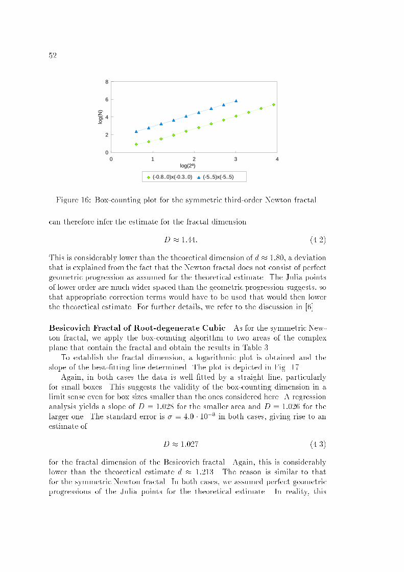
520 1 2 3 4

0

2

4

6

8

log(2ª)

log(

N)

(-0.8..0)x(-0.3..0) (-5..5)x(-5..5)Figure 16: Box-counting plot for the symmetric third-order Newton fractalcan therefore infer the estimate for the fractal dimensionD � 1:44: (4.2)This is considerably lower than the theoretical dimension of d � 1:80, a deviationthat is explained from the fact that the Newton fractal does not consist of perfectgeometric progression as assumed for the theoretical estimate. The Julia pointsof lower order are much wider spaced than the geometric progression suggests, sothat appropriate correction terms would have to be used that would then lowerthe theoretical estimate. For further details, we refer to the discussion in [6].Besicovich Fractal of Root-degenerate Cubic As for the symmetric New-ton fractal, we apply the box-counting algorithm to two areas of the complexplane that contain the fractal and obtain the results in Table 3.To establish the fractal dimension, a logarithmic plot is obtained and theslope of the best-�tting line determined. The plot is depicted in Fig. 17.Again, in both cases the data is well �tted by a straight line, particularlyfor small boxes. This suggests the validity of the box-counting dimension in alimit sense even for box sizes smaller than the ones considered here. A regressionanalysis yields a slope of D = 1:028 for the smaller area and D = 1:026 for thelarger one. The standard error is � = 4:0 � 10�3 in both cases, giving rise to anestimate of D � 1:027 (4.3)for the fractal dimension of the Besicovich fractal. Again, this is considerablylower than the theoretical estimate d � 1:213. The reason is similar to thatfor the symmetric Newton fractal. In both cases, we assumed perfect geometricprogressions of the Julia points for the theoretical estimate. In reality, this

53[0:75; 1:5]� [0; 1:8] [0; 2]� [�2; 2]a box counts Na(A) total boxes Na(A) total boxes2 10 24 28 1283 23 90 56 5124 44 348 108 20485 87 1392 218 81926 188 5568 478 32 7687 390 22 176 984 131 0728 768 88 512 1946 524 2889 1572 354 048 3968 2 097 15210 3201 1 416 192 8076 8 388 60811 6451 5 663 232 16 262 33 554 43212 13 069 22 64 856 33 022 134 217 72813 26 412 90 599 424Table 3: Box-counting results for the Besicovich fractal0 1 2 3 4

0

1

2

3

4

5

log(2ª)

log(

N)

(0.75..1.5)x(0..1.8) (0..2)x(-2..2)Figure 17: Box-counting plot for the Besicovich fractalassumption only holds for high-order Julia points and is violated considerablyin the beginning of a chain of Julia points. We postulate that by introducingproper correction terms for this phenomenon, the theoretical estimate will getsmaller and into better agreement with the box-counting results.

544.2 Analysis of Local Solvers for the Turbulent k � �EquationsOne of the most commonly used models in turbulence computations is the k� �model introduced by Jones and Launder (for a derivation, see e.g. [8]). Itamends the Navier-Stokes equations for uid ow with two transport equations,introducing the quantities k and � that describe the turbulent ow features.The employed approximation of the Reynolds stress tensor assumes isotropy, arestriction that limits the practical accuracy of the model. However, it is widelyused due to its relative computational ease.Despite the possibility of using a stabilised form of Newton's method as aglobal solver for the k�� equations [5], most available software uses time-steppingtechniques and solves the equations pointwise. It is common to locally decouplethe turbulence equations from the Navier-Stokes equations, establishing a nestediteration that only solves one system of equations at a time. In this context, weare interested in the nonlinearity introduced by the k � � system. In symbolicnotation, this system can be written asc1k2 + c2k�+ c3�+ c4�2 = 0 (4.4a)d1k2 + d2k�+ d3k + d4�2 = 0; (4.4b)and is solved for fk; �g. Usually, Newton's method is used for this purpose.The coe�cients are real and �xed for each point, but as they are determined bythe ow variables, they vary considerably across the geometry. To analyse theproperties of the system (4.4), we eliminate one of the variables to obtain�c21 �b0 + b1�+ b2�2 + b3�3� = 0; (4.5)with the coe�cientsb0 = c1c3d23b1 = c3d1(c3d1 � c2d3) + c1d3(2c3d2 + c4d3)b2 = c3d1(2c4d1 � c2d2 � 2c1d4) + c1d2(c3d2 + 2c4d3)�c2d3(c4d1 + c1d4)b3 = (c1d4 � c4d1)2 + (c4d2 � c2d4)(c1d2 � c2d1): (4.6)The spurious, turbulence-free solution fk; �g = f0; 0g can be eliminated from(4.5), yielding the cubic b0 + b1�+ b2�2 + b3�3 = 0: (4.7)As the coe�cients are real, this corresponds to the general cubic discussed inthe previous section. As mentioned above, the coe�cients of this cubic containinformation about the ow variables and are therefore likely to vary considerably

55throughout the geometry. In particular, all di�erent fractal forms discussed forthe general cubic are likely to appear, if � would be a complex variable. However,the Newton search is con�ned to the real axis only and we are therefore interestedin the one-dimensional Julia set of the fractals that resides on the real axis. Thiswill determine the convergence behaviour of Newton's method when started to�nd a real root of (4.5). In general, the more Julia points are found on the realaxis, the longer the convergence history will be, as the vicinity of any Julia pointwill be subject to large Newton shifts eventually.Following the discussion in the previous section, we can distinguish threecases, depending on the roots �i of (4.7) and the roots �i of the derivative withrespect to �.� f�ig 2 R: The real axis contains two Julia points with same modulus andopposite sign.� �1 2 R; �2;3 2 C; �i 2 C: The real axis contains no Julia points.� �1 2 R; �2;3 2 C; �i 2 R: The real axis contains an in�nite number ofJulia points left of �1 > 0.Of this list, only the last case will pose problems for a considerable range ofstarting values, where it will be quite likely that Newton's method gets close toa Julia point and therefore takes a long time converging with a linear rate (seethe discussion in [6] for a more detailed explanation). Furthermore, the Juliapoints are in a positive region where physical intuition would suggest suitableguesses for the solution - starting from little turbulence, close to the origin. Itis therefore very advisable that a local Newton solver in a k� � code avoids thiscritical region. This can be done by choosing a starting value that is boundedfrom below by �(0) > �1 = 16b3 ��2b2 +q4b22 � 12b1b3� : (4.8)Relying only on the known coe�cients of (4.4), this estimate can be obtainedat little computational cost. As the bound gives the coordinate of the largestJulia point, it is not advisable to start too close to it. Any positive correction ofthe bound, however, does not impair convergence dramatically as starting valueswith �(0) > �1 are located in the convex region of (4.7) and therefore convergedirectly to the root.Numerical results for an exemplary cubic of the formx3 � x� 1 = 0 (4.9)with a real root at x = 1:3247179 con�rm this theoretical bound. We consideredthree intervals in which we started Newton's method for a sequence of equallyspaced initial guesses and counted the iterations until convergence with a residual

56of 10�13. Table 4 states the results. In addition to the average iteration count xuntil convergence, we state the empirical variance for n runss2 = 1n� 1 nXi=1 (xi � x)2 (4.10)as a measure on the predictability of the convergence history. The number ofinitial guesses n = 577 was held constant throughout the experiment. Timingwas done on an Intel 80486 based system, for 50 runs to convergence on eachguess and then scaled down for one run, yielding the �gure stated. As a repre-sentative of a commonly used stabilisation technique, dynamic shift scaling forthe downward shifts was implemented with the limiting value as stated. For adetailed discussion of the stability issues of that method in a fractal context, see[6]. Interval iterations x variance s2 time [sec] method0.001, 0.577 24.54 227.593 0.30 orthodox109.96 0.037 1.46 scaling 0.999160.96 0.037 1.84 scaling 0.990.600, 1.176 6.73 3.069 0.11 orthodox6.67 2.546 0.12 scaling 0.9996.67 2.546 0.12 scaling 0.995.000, 5.576 8.00 0.000 0.12 orthodox8.00 0.000 0.13 scaling 0.99Table 4: Convergence for various starting guesses on a k � � type cubicThe �rst interval is entirely located left of the primary Julia point �0 = 1p3.The orthodox method exhibits a large variance - indicator for the presence ofmany Julia points - and a large number of iterations to converge on averagefor a starting guess. A closer survey of the convergence path shows that largeshifts occur and the iterates are often negative. The chosen shift limits for thedownward shift scaling prevent negative iterates, and increase predictability ofconvergence. This however happens at the expense of dramatically slow conver-gence. The improved predictability of the stabilised method is coherent with theresults on fractal depletion presented in [6].The second interval is located just above the bound given in (4.8), and dis-plays improved convergence in every aspect. The runtime gain shows almost afactor of 3, as does the gain in iterations. As the interval is rather close to theroot, iteration counts vary due to normal Newton convergence, thus the value ofthe variance. It is noted that even for the orthodox method, the iterates staypositive, and shift scaling can be employed at almost no additional cost.

57The third interval shows that it is safe to use the physically counterintuitiveapproach of choosing large starting values and exploiting the convexity of thefunction. Despite an initial error that is much larger than for the �rst interval,convergence compares to the case of starting very close to the root in the secondinterval. With the interval being further from the root, all guesses converge inthe same number of iterations, thus the vanishing variance.

585 Concluding RemarksIn this work, we have examined the properties of Newton's method employedto �nd the roots of complex polynomials numerically. For the symmetric casez� � 1, a generation mechanism for the resulting fractal structure has been es-tablished from �rst principles, yielding quantitative results for the properties ofthe structure.The results generalise from the case � = 3, where a connection between thefractal generation mechanism and numerical convergence from any starting pointwas established in [6]. As the generation principle is conserved, the numericalconvergence pattern is conserved as well. We can state that converging from anystarting point for any complex polynomial of order �, the residual convergencepath of Newton's method obeys the following four distinct patterns.� A stationary residual with magnitude de�ned by the primary Julia point�0 and the �rst-order Julia point �1, when the iterates move within theparent structure and constantly change the fractal branch.� A sharp increase in residual, when the iterates leave the parent structurewith a change of branch. This has to be followed by� Linear convergence with an approximate rate ��1� as the iterates movelaterally along one branch. This is the only type of convergence possibleoutside the parent structure for large iterates.� Quadratic convergence once the iterates get su�ciently close to the rootfor classical Newton-Kantorovich stability to hold.For symmetric polynomials, the �rst statement translates into 'stationaryresidual with magnitude 1'. For general polynomials, the factor for linear con-vergence holds as their global behaviour is determined by the highest order � ofthe variable (see the general cubic for an example). We can therefore concludethat for general complex polynomials, the global numerical convergence path ofNewton's method is explicable once the underlying fractal structure of the prob-lem is known. It is likely that these principles generalise to other functions, butwe have no quantitative results there.Discussing the general cubic problem, a comprehensive description of thepossible fractal structures for third-order polynomials has been stated. As thisdescription gives bounds on the location of the numerically critical Julia points,it can be used to speed up numerical computations involving the solution ofcubics. A straightforward example for the k�� equations in turbulence modellinghas been presented. Of course, the results can be applied to any other two-dimensional polynomial system of overall degree 3 (i.e. that can be transformedinto a complex cubic).

59It is expected that a general description of the fractal structures is also pos-sible for systems of degree four due to the existence of analytic formuli for thesolution. The derivation of this description would be technically equivalent tothe cubic case and was therefore omitted in this work. However, it should bestraightforward to implement it using the concepts presented here.For systems with degree larger than four, no analytic solution exists in gen-eral. The discussion will therefore most likely be restricted to the symmetriccase, where this work has given a comprehensive list of properties. The fractaldimension can be estimated numerically, determining the necessary scale factorsvia computation.In determining the fractal properties of symmetric polynomials in associationwith Newton's method, a gap in the subject of fractal geometry has been closed.Furthermore, by analysing the general cubic, applications of the fractal theory topractical systems of equations have been made possible. It was established thatthe results concerning the fractal properties can be applied directly to understandand improve numerical convergence. We feel that the results obtained for thestill rather simple case of polynomials might generalise for other, more di�cultclasses of problems and help to improve the adaptions of Newton's method forengineering and physics applications.AcknowledgementsThis work was �nished while M. Drexler was visiting the program of Scienti�cComputing / Computational Mathematics at Stanford University. He wouldlike to express his gratitude to Prof. G.H. Golub for the kind invitation andthe academic support at Stanford. He also wants to thank M. Gander (SC/CM,Stanford) for helpful discussions. The �nancial support of the German AcademicExchange Service (DAAD) through the programme HSPII/AUFE is acknowl-edged gratefully.C. Bracher acknowledges the �nancial support of the 'Studienstiftung desdeutschen Volkes'.

60References[1] Abramowitz, M. and Stegun, I. Handbook of Mathematical Functions.Dover. New York. 1972.[2] Barnsley, M. Fractals everywhere. Academic Press. London. 1988.[3] Blanchard, P. and Chiu, A. Complex Dynamics: An Informal Discussion.in: B�elair, J. and Dubuc, S. Fractal Geometry and Analysis. NATO-ASIseries, Kluwer Academic Publishers. 1991.[4] Douady, A. Syst�emes dynamiques holomorphes. S�eminaire Bourbaki,No. 599. 1983.[5] Drexler, M. and Rollett, J.S. An adapted Newton Method for the turbulentk � � Equations. in: Morton, K.W. and Baines, M.J. Numerical Methodsfor Fluid Dynamics. Oxford University Press. 1996.[6] Drexler, M., Sobey, I.J. and Bracher, C. On the Fractal Characteristics ofa Modi�ed Newton Method. Numerical Analysis Group Oxford. TechnicalReport 95/26.[7] Falconer, K. Fractal Geometry. John Wiley and Sons. Chichester. 1990.[8] Gwilliam, C.S. Parallel Algorithms for Navier-Stokes Modelling.D.Phil. the-sis. Numerical Analysis Group, University of Oxford. 1993.[9] Golub, G.H. and van Loan, C.F.Matrix Computations. Johns Hopkins Uni-versity Press. 2nd edition. 1989.[10] Henrici, P. Applied and Computational Complex Analysis. Volume 1. JohnWiley and Sons. New York. 1974.[11] Julia, G. Sur l'iteration des fonctions rationelles. Journal de Math�ematiquesPure et Appliqu�ee s�er. 8, 47-245. 1918.[12] Knoll, D.A. and McHugh, P.R.An inexact Newton Algorithm for Solving theTokamak Edge Plasma Fluid Equations on a Multiply-Connected Domain.Journal of Computational Physics 116, pp. 281-291. 1995.[13] Mandelbrot, B. The Fractal Geometry of Nature. W.H. Freeman and Com-pany. New York. 1983.[14] Manning, A. How to be sure of �nding a root of a complex polynomial usingNewton's method. Boletim da Sociedade Brasileira de Matem�atica, Vol. 22,No. 2, pp. 157-177. 1992

61[15] Marden, M. Geometry of Polynomials. Second Edition. American Mathe-matical Society. Providence, Rhode Island. 1966.[16] Ortega, J. and Rheinboldt, W. Iterative Solution of Nonlinear Equations inSeveral Variables. Academic Press. New York. 1970.[17] Peitgen, H.O. and Saupe, D. The Science of Fractal Images. Springer-Verlag.New York. 1988.[18] Peitgen, H.O., Saupe, D. and Haeseler, F.v. Cayley's Problem and JuliaSets. The Mathematical Intelligencer Vol. 6, No. 2. Springer-Verlag. NewYork. 1984.[19] Press, W.H., Flannery, B.P., Teukolsky, S.A. and Vetterling, W.T. Numeri-cal Recipes in Fortran. Cambridge University Press. 2nd edition. 1993.[20] Smale, S. The Fundamental Theorem of Algebra and Complexity Theory.Bulletin of the American Mathematical Society Vol. 4, No. 1, pp. 1-36. 1981.[21] Stoer, J. and Bulirsch, R. Introduction to Numerical Analysis. Translatedby R. Bartels, W. Gautschi, C. Witzgall. Springer-Verlag. New York. 1980.