Physics Letters B 695 (2011) 247–251

Contents lists available at ScienceDirect

Physics Letters B

www.elsevier.com/locate/physletb

Renormalized field strength correlators in SU(N) gauge theory and gauge/stringduality

Oleg Andreev 1

Arnold Sommerfeld Center for Theoretical Physics, LMU-München, Theresienstrasse 37, 80333 München, Germany

a r t i c l e i n f o a b s t r a c t

Article history:Received 26 May 2010Received in revised form 31 August 2010Accepted 11 November 2010Available online 13 November 2010Editor: L. Alvarez-Gaumé

Keywords:QCDField strength correlatorsGauge/string duality

We use gauge/string duality to analytically evaluate correlation lengths of the renormalized field strengthcorrelators in pure Yang–Mills theories at zero and finite temperature.

© 2010 Elsevier B.V. All rights reserved.

1. Introduction

Understanding the infrared behavior of gauge theories from firstprinciples is a longstanding problem that offers perhaps the besthope of eventually understanding all the mysteries of quantumchromodynamics (QCD). It is well known that an important classof gauge invariant correlation functions in the QCD vacuum is con-structed from field strengths and Wilson lines. These correlators doplay an important role in several areas of QCD including modelsof stochastic confinement of color, high energy scattering, heavyquarkonium systems, etc.2

The simplest field strength correlator in four-dimensional Eu-clidean space is defined by

Dμν,ρτ (x) = ⟨tr

[Gμν(0)U P (0, x)Gρτ (x)U P (x,0)

]⟩. (1)

Here xμ are the Euclidean coordinates, the trace is over the fun-damental representation, Gμν is a field strength of the gauge fieldAμ and U P (x,0) is a path-ordered Wilson line. The last is defined

as U P (x1, x2) = P exp[ig ∫ 10 ds dxμ

ds Aμ(x(s))], where s is a parame-ter of the path running from 0 at x = x1 to 1 at x = x2 and g is agauge coupling constant.3 The paths are defined as straight lines.

If one considers not a field strength but a field with differ-ent color quantum numbers, then the construction of correlators

E-mail address: andre@itp.ac.ru.1 Also at Landau Institute for Theoretical Physics, Moscow.2 The literature on the field strength correlators is vast. For a review, see, e.g., [1]

and references therein.3 In what follows we omit the indices when it is clear from the context.

0370-2693/$ – see front matter © 2010 Elsevier B.V. All rights reserved.doi:10.1016/j.physletb.2010.11.029

is changed. For instance, a field transforming in the fundamentalrepresentation of the gauge group will produce a two-point corre-lator

Ψ (x) = ⟨q̄(0)U P (0, x)q(x)

⟩, (2)

with q the field in the fundamental representation of SU(N) andq̄ its conjugate. In general, there are many possible generalizationsof the correlators by choosing different (curved) contours for theWilson lines, or by inserting operators along the contours.

It is believed that for large separation of the field strength op-erators the two-point correlator falls off exponentially [1]

Dμν,ρτ (x) ∼ Pμν,ρτ e− rλ , (3)

where Pμν,ρτ is a kinematical factor, r = √(xμ)2, and λ is a corre-

lation length. This is the case also for Ψ , in fact

Ψ (x) ∼ e− rξ , (4)

with a correlation length ξ .Until recently, the lattice formulation, still struggling with lim-

itations and system errors, was the main computational tools todeal with non-weakly coupled gauge theories. The field strengthcorrelators were also intensively studied (for a brief review, see[2]). The situation changed drastically with the invention of theAdS/CFT correspondence [3] that resumed interest in another tool,string theory. The original duality was for conformal theories, butvarious perturbations (deformations) produce gauge/string dualswith a mass gap, confinement, chiral symmetry breaking, etc. [4].

In this Letter we continue a series of recent studies devoted toa search for an effective string description of pure gauge theories.

248 O. Andreev / Physics Letters B 695 (2011) 247–251

In [5], the model was presented for computing the heavy quarkpotential at zero temperature. Subsequent comparison [6] with theavailable lattice data has made it clear that the model should betaken seriously. A non-trivial cross check for this model [7], whichchecked the phenomenological value of the gluon condensate [8],was also carried out. Later, the model was extended to finite tem-perature. The results obtained for the spatial string tension [9] andthe expectation value of the renormalized Polyakov loop [10] inthe deconfined phase are remarkably consistent with the lattice,too. As is known, QCD is a very rich theory supposed to describethe whole spectrum of strong interaction phenomena. The questionnaturally arises: How well does such an effective string descriptioncapture other aspects of quenched QCD? Here, we address the is-sue of computing the field strength correlators in an analytical wayas an important step toward answering this question.4

Before proceeding to the detailed analysis, let us set the basicframework. As in [5,7], we take the following ansatz for the five-dimensional background geometry

ds2 = GN M dX N dX M = R2 w(dt2 + d�x2 + dz2), w(z) = esz2

z2

(5)

to describe a pure gauge theory at zero temperature. The metric(5) is that of a deformed AdS5 space, where s is a deformationparameter whose value can be fixed, for example, from the heavyquark potential. We take a constant dilaton and discard other back-ground fields.

When we go to the deconfined phase, we consider the five-dimensional geometry of [9,10]

ds2 = GN M dX N dX M = R2 w

(f dt2 + d�x2 + 1

fdz2

),

f (z) = 1 −(

z

zT

)4

, (6)

which represents a deformed Schwarzschild black hole in AdS5space. Here zT is related to the Hawking temperature T = 1/(π zT)

whose dual description is nothing but the temperature of gaugetheory.

2. Calculating the correlators at zero temperature

To begin with, we need to find a recipe for computing the fieldstrength correlators within the gauge/string duality. The strategyfor finding it is as follows. In discussing the Wilson loops [11], onefirst chooses a contor C on a four-manifold which is the boundaryof a five-dimensional manifold. Next, one has to study fundamentalstrings on this manifold such that the string world-sheet has C asits boundary. The expectation value of the Wilson loop is schemat-ically given by the world-sheet path integral 〈W (C)〉 = ∫

D Xe−S w ,where X denotes a set of world-sheet fields and S w is a world-sheet action. In principle, the integral can be evaluated approxi-mately in terms of minimal surfaces that obey the boundary con-ditions. The result is written as 〈W (C)〉 = ∑

n wne−Sn , where Sn

means a renormalized minimal area (in string units) whose weightis wn .

In the case of a rectangular Wilson loop living on the bound-ary (z = 0) of five-dimensional space (5) a minimal surface cor-responding to a static string configuration is sewn together fromthree surfaces, as shown in Fig. 1 (left). For large T , we have [5]

4 To our knowledge, there have been no studies (numerical or analytical) of thisissue from the viewpoint of AdS/CFT, or gauge/string duality, in the literature.

Fig. 1. Left: A minimal surface for a rectangular loop C indicated by thick lines alongthe (t, x)-axes. It includes a lateral surface whose area is proportional to T and twoidentical end-surfaces with areas independent of T . Right: The end-surface in thex–z plane. It is bounded by a curved profile of a static string stretched betweenquark sources set at x = 0, r and a straight Wilson line indicated by a thick linealong the x-axis. Note that in the model we are considering a gravitational forceprevents the string from getting deeper than zc = 1/

√s into z direction [5].

⟨W (C)

⟩ � e−E T −2S , (7)

where E is a ground state energy of a quark–antiquark bound stateand S is a renormalized area of the end-surface shown in Fig. 1(right).

On the other hand, in the temporal gauge the expectation valueof the Wilson loop can be evaluated as5

⟨W (C)

⟩ � 〈ψ |e−H T |ψ〉 = e−E T Ψ 2(r), (8)

where H is the gauge Hamiltonian in the temporal gauge and |ψ〉is the quark–antiquark bound state. It is given by |ψ〉 = Ψ (r) :q̄(r)U P (r,0)q(0) : |0〉 such that 〈0| : q̄(r)U P (r,0)q(0) : |0〉 = 1. Sincethe quarks are non-dynamic, we need to normal order only the P -exponential function that results in non-zero expectation value forthe normal ordered operator. Note that the exponential fall off (4)is consistent with the fact that |ψ〉 is normalizable.

Then combining this with (7), we find

Ψ (r) � e−S , (9)

where S is a renormalized area of the surface shown in Fig. 1(right). Note that this formula is valid only for the ground state.

It is worth noting that a similar representation has been sug-gested in [13] for the expectation value of the Polyakov loop. Inthis case there is no need for the quark sources. The string is pre-vented from getting deep into z direction by a black hole geometrysuch that the maximum value of z is bounded by the black holehorizon. In the model with dynamic quarks it appeared in [14].A difference here is that the Wilson loop goes along an internaldirection. In general, it is natural to expect that in the presence ofdynamic quarks the representation (9) breaks down at large sep-arations due to string breaking. Physically, this means that quarkbound states decay.

To write a formal expression for the field strength correlator (1),let us think of the Wilson lines as forming a long, narrow rectangu-lar loop in the x–t plane, as shown in Fig. 1 (left) but with small T .The field strength operators are set at (0,0) and (r,0). The expo-nential fall off (3) for large r is due to the Wilson loop expectationvalue. Subleading corrections come from quadratic fluctuations inthe world-sheet path integral and from the field strength opera-tors. They are expected to give a polynomial prefactor P in front ofthe exponential. Taking the limit T → 0, we have

Dμν,ρτ (r) ∼ Pμν,ρτ e−2S , (10)

where S is the same renormalized area as in (9). Note that thisformula only provides the leading exponent in the large r limit.

5 For example, see [12] and references therein.

O. Andreev / Physics Letters B 695 (2011) 247–251 249

In analyzing the formulas (9) and (10), an interesting relationarises. Since S is proportional to r, we find that the correlationlengths ξ and λ are related as

λ = 1

2ξ. (11)

Given the background metric, we can calculate the renormal-ized area S by using the exact shape of the static string stretchedbetween the heavy quark sources [5]. With the large r behavior inmind, it is technically suitable to add two pieces, shown in dashedlines in Fig. 1 (right), to the original surface. Their areas are eachof subleading order in 1/r. As a result, the surface of interest be-comes a rectangular in the x–z plane.

Now we are ready to use the Nambu–Goto action equippedwith the background metric (5)

S = 1

2πα′

∫d2τ

√det GN M∂α X N∂β X M . (12)

Next, we choose τ 1 = x and τ 2 = z. This yields

S = g

πr

zc∫0

dz w = g

π

r

zc

1∫0

du w(u), (13)

where g = R2

2α′ and zc = 1√s

. We have also rescaled z as z = zcu.

Since the integral is divergent at u = 0 due to the z−2 factor in themetric, we have to regularize it. We do so by imposing a cutoff ε .

To next-to-leading order in ε , the integral is given by

1∫ε

du w = 1

ε+ √

π Erfi(1) − e + O (ε), (14)

where Erfi(x) is the imaginary error function. We use the mod-ified minimal subtraction scheme to deal with this integral.6 So,we subtract the power divergence 1/ε together with a constant cwhose value must be specified from renormalization conditions. Asa result, the renormalized area takes the form7

S = g

π

√sr

(c + √

π Erfi(1) − e). (15)

Combining this with (4) and (9), we get the correlation length ξ

ξ = π

g√

s

(c + √

π Erfi(1) − e)−1

. (16)

It is now clear that T must go to zero faster than ε . Indeed, inthe limit T /ε → 0 the contribution of the lateral surface vanishesand, as a consequence, the relation (10) holds. With this fact un-derstood, it is now straightforward to find the correlation length λ

λ = π

2g√

s

(c + √

π Erfi(1) − e)−1

. (17)

To define the model properly, we must specify the renormaliza-tion conditions. In doing so, we start with the correlation length ξ .Our stringy construction suggests a natural condition ξ = 1/

√σ ,

where σ is the string tension. In the model we are consideringit is given by σ = egs/π [5]. Making an estimate requires some

6 Note that the use of the modified minimal subtraction scheme in [5] allows oneto adjust the value of a constant in the potential. Moreover, it also helps in findinga relation between the gauge/string duality result of [10] and the lattice data forthe renormalized Polyakov loop.

7 Of course, the constant part being a number (√

π Erfi(1) − e) can be absorbedinto c. However, it becomes temperature-dependent at finite temperature (as wewill see in Section 3), so we keep it.

numerics. For SU(3) a value of g fixed from the heavy quark po-tential is g ≈ 0.62 [6]. This gives c ≈ 3.50. A typical value of s iss ≈ 0.45 GeV2 [6,15]. If so, a value of λ is estimated to be

λ ≈ 0.20 fm. (18)

Is it a reasonable value? Although the lattice calculations of [16]claim a slightly bigger value λ ≈ 0.22 fm but with an error of order0.03 fm, there is an obvious troublesome question. If the calcula-tions are made in two different renormalization schemes, why arethe results so similar? Unfortunately, we have no real resolution ofthis problem.

On the other hand, choosing λ = m−1G , with mG ≈ 3.64

√σ the

mass of the lightest glueball [17], gives c ≈ 5.62. A simple algebrashows that in this case λ ≈ 0.13 fm.

3. Calculating the correlators at finite temperature

According to [1], at finite temperature we must separately con-sider the electric and magnetic correlators [1]. So, we decomposeGμν into the electric and magnetic fields: Ei = G0i and Bi =12 εi jkG jk . It is expected [18] that at large separations the magneticcorrelators show exponential fall off for any temperature, while theelectric ones do so just below the critical temperature Tc .

To study the magnetic correlator D(m)i j (x) = 〈tr[Bi(0, �x)U P (x,0)×

B j(0,0)U P (0, x)]〉, we take the Wilson lines in the x–y plane andregard C as a long, narrow rectangle similar to that of Fig. 1 (witht replaced by y). Thus, C is now a spatial Wilson loop. A crucialdifference from temporal Wilson loops is that in the deconfinedphase spatial ones obey an area law, with a spatial string tensionσs .8 In other words, a (spatial) string stretched between two well-separated sources doesn’t break. This allows us to use a formalismsimilar to that of Section 2. So, the exponential fall off for large ris due to the spatial Wilson loop expectation value. The magneticfield operators and world-sheet fluctuations contribute to a poly-nomial prefactor P in front of the exponential. Taking the T → 0limit, we find

D(m)i j (r) ∼ Pi je

−2S , (19)

where S is a renormalized area of the surface shown in Fig. 1(right).

Repeating the arguments of Section 2, we add two pieces to theoriginal surface to simplify further calculations. The Nambu–Gotoaction, which we wrote before as (12), is now

S = 1

2πα′

∫d2τ

√det GN M∂α X N∂β X M , (20)

where the background metric G is given by (6). Using the gaugeτ 1 = x and τ 2 = z, it becomes

S = g

πr

zT∫0

dzw√

f= g

π

r

zT

1∫0

dvw√

f(v). (21)

Here we have rescaled z as z = zT v . As in Section 2, we regular-ize the integral over v by imposing a cutoff ε . Note that in thedeconfined phase the large distance physics is determined by thenear horizon geometry of the deformed Schwarzschild black holein AdS5 space [9,13]. So, the upper limit is zT.

8 Recall that σs is not a physical string tension because it is not related to theproperties of a physical potential.

250 O. Andreev / Physics Letters B 695 (2011) 247–251

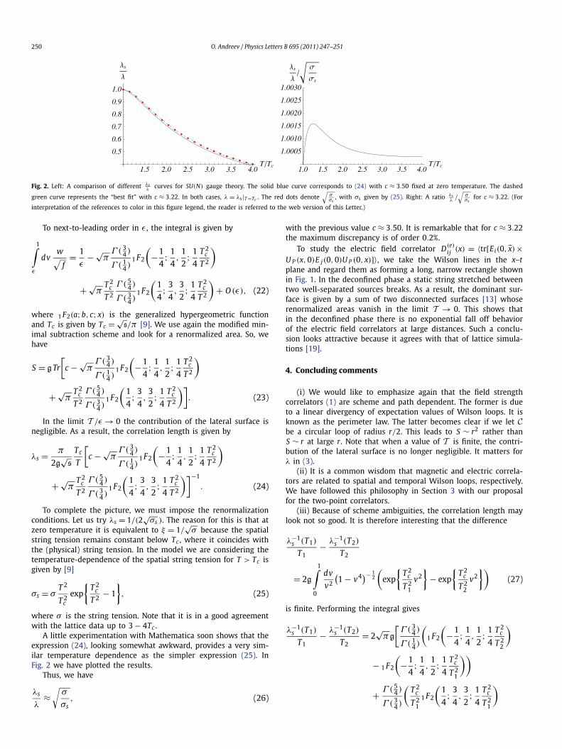
Fig. 2. Left: A comparison of different λsλ

curves for SU(N) gauge theory. The solid blue curve corresponds to (24) with c ≈ 3.50 fixed at zero temperature. The dashed

green curve represents the “best fit” with c ≈ 3.22. In both cases, λ = λs|T =Tc . The red dots denote√

σσs

, with σs given by (25). Right: A ratio λsλ

/√

σσs

for c ≈ 3.22. (For

interpretation of the references to color in this figure legend, the reader is referred to the web version of this Letter.)

To next-to-leading order in ε , the integral is given by

1∫ε

dvw√

f= 1

ε− √

πΓ ( 3

4 )

Γ ( 14 )

1 F2

(−1

4; 1

4,

1

2; 1

4

T 2c

T 2

)

+ √π

T 2c

T 2

Γ ( 54 )

Γ ( 34 )

1 F2

(1

4; 3

4,

3

2; 1

4

T 2c

T 2

)+ O (ε), (22)

where 1 F2(a;b, c; x) is the generalized hypergeometric functionand Tc is given by Tc = √

s/π [9]. We use again the modified min-imal subtraction scheme and look for a renormalized area. So, wehave

S = gTr

[c − √

πΓ ( 3

4 )

Γ ( 14 )

1 F2

(−1

4; 1

4,

1

2; 1

4

T 2c

T 2

)

+ √π

T 2c

T 2

Γ ( 54 )

Γ ( 34 )

1 F2

(1

4; 3

4,

3

2; 1

4

T 2c

T 2

)]. (23)

In the limit T /ε → 0 the contribution of the lateral surface isnegligible. As a result, the correlation length is given by

λs = π

2g√

s

Tc

T

[c − √

πΓ ( 3

4 )

Γ ( 14 )

1 F2

(−1

4; 1

4,

1

2; 1

4

T 2c

T 2

)

+ √π

T 2c

T 2

Γ ( 54 )

Γ ( 34 )

1 F2

(1

4; 3

4,

3

2; 1

4

T 2c

T 2

)]−1

. (24)

To complete the picture, we must impose the renormalizationconditions. Let us try λs = 1/(2

√σs ). The reason for this is that at

zero temperature it is equivalent to ξ = 1/√

σ because the spatialstring tension remains constant below Tc , where it coincides withthe (physical) string tension. In the model we are considering thetemperature-dependence of the spatial string tension for T > Tc isgiven by [9]

σs = σT 2

T 2c

exp

{T 2

c

T 2− 1

}, (25)

where σ is the string tension. Note that it is in a good agreementwith the lattice data up to 3 − 4Tc .

A little experimentation with Mathematica soon shows that theexpression (24), looking somewhat awkward, provides a very sim-ilar temperature dependence as the simpler expression (25). InFig. 2 we have plotted the results.

Thus, we have

λs ≈√

σ, (26)

λ σs

with the previous value c ≈ 3.50. It is remarkable that for c ≈ 3.22the maximum discrepancy is of order 0.2%.

To study the electric field correlator D(e)i j (x) = 〈tr[Ei(0, �x)×

U P (x,0)E j(0,0)U P (0, x)]〉, we take the Wilson lines in the x–tplane and regard them as forming a long, narrow rectangle shownin Fig. 1. In the deconfined phase a static string stretched betweentwo well-separated sources breaks. As a result, the dominant sur-face is given by a sum of two disconnected surfaces [13] whoserenormalized areas vanish in the limit T → 0. This shows thatin the deconfined phase there is no exponential fall off behaviorof the electric field correlators at large distances. Such a conclu-sion looks attractive because it agrees with that of lattice simula-tions [19].

4. Concluding comments

(i) We would like to emphasize again that the field strengthcorrelators (1) are scheme and path dependent. The former is dueto a linear divergency of expectation values of Wilson loops. It isknown as the perimeter law. The latter becomes clear if we let Cbe a circular loop of radius r/2. This leads to S ∼ r2 rather thanS ∼ r at large r. Note that when a value of T is finite, the contri-bution of the lateral surface is no longer negligible. It matters forλ in (3).

(ii) It is a common wisdom that magnetic and electric correla-tors are related to spatial and temporal Wilson loops, respectively.We have followed this philosophy in Section 3 with our proposalfor the two-point correlators.

(iii) Because of scheme ambiguities, the correlation length maylook not so good. It is therefore interesting that the difference

λ−1s (T1)

T1− λ−1

s (T2)

T2

= 2g

1∫0

dv

v2

(1 − v4)− 1

2

(exp

{T 2

c

T 21

v2}

− exp

{T 2

c

T 22

v2})

(27)

is finite. Performing the integral gives

λ−1s (T1)

T1− λ−1

s (T2)

T2= 2

√πg

[Γ ( 3

4 )

Γ ( 14 )

(1 F2

(−1

4; 1

4,

1

2; 1

4

T 2c

T 22

)

− 1 F2

(−1

4; 1

4,

1

2; 1

4

T 2c

T 21

))

+ Γ ( 54 )

Γ ( 3 )

(T 2

c

T 2 1 F2

(1

4; 3

4,

3

2; 1

4

T 2c

T 2

)

4 1 1

O. Andreev / Physics Letters B 695 (2011) 247–251 251

− T 2c

T 22

1 F2

(1

4; 3

4,

3

2; 1

4

T 2c

T 22

))]. (28)

Thus, our model predicts the scheme-independent relation be-tween the correlation lengths of magnetic operators at differenttemperatures. It will be interesting to see whether it will match orclose to match lattice simulations.

(iv) If we consider not a field strength but an arbitrary local op-erator in the adjoint representation of SU(N), then it follows fromour proposal that the correlator shows the exponential fall off

⟨O(0)U P (0, x)O(x)U P (x,0)

⟩ ∼ e− rλ for r → ∞, (29)

with a universal correlation length λ.

Acknowledgements

This work was supported in part by DFG within the Emmy-Noether-Program under Grant No. HA 3448/3-1 and the Alexandervon Humboldt Foundation under Grant No. PHYS0167. We wouldlike to thank P. de Forcrand, M. Haack, A.I. Vainstein, V.I. Za-kharov, and especially P. Weisz for useful discussions and com-ments. We also acknowledge the warm hospitality at Yukawa In-stitute for Theoretical Physics, where a portion of this work wasdone.

References

[1] A. Di Giacomo, H.G. Dosch, V.I. Shevchenko, Yu.A. Simonov, Phys. Rep. 372(2002) 319;A.M. Badalian, Yu.A. Simonov, V.I. Shevchenko, Phys. Atom. Nucl. 69 (2006)1781;A.M. Badalian, Yu.A. Simonov, V.I. Shevchenko, Yad. Fiz. 69 (2006) 1818.

[2] A. Di Giacomo, M. D’Elia, H. Panagopoulos, E. Meggiolaro, Gauge invariant fieldstrength correlators in QCD, hep-lat/9808056.

[3] J.M. Maldacena, Adv. Theor. Math. Phys. 2 (1998) 231;S.S. Gubser, I.R. Klebanov, A.M. Polyakov, Phys. Lett. B 428 (1998) 105;E. Witten, Adv. Theor. Math. Phys. 2 (1998) 253.

[4] For a review, see, O. Aharony, S.S. Gubser, J.M. Maldacena, H. Ooguri, Y. Oz,Phys. Rep. 323 (2000) 183;See also for an updated reference list: R.C. Myers, S.E. Vazquez, Class. Quant.Grav. 25 (2008) 114008;S.S. Gubser, A. Karch, Ann. Rev. Nucl. Part. Sci. 59 (2009) 145;S.J. Brodsky, G. de Teramond, arXiv:1001.1978.

[5] O. Andreev, V.I. Zakharov, Phys. Rev. D 74 (2006) 025023.[6] C.D. White, Phys. Lett. B 652 (2007) 79.[7] O. Andreev, V.I. Zakharov, Phys. Rev. D 76 (2007) 047705.[8] M.A. Shifman, A.I. Vainstein, V.I. Zakharov, Nucl. Phys. B 147 (1979) 385;

M.A. Shifman, A.I. Vainstein, V.I. Zakharov, Nucl. Phys. B 147 (1979) 448.[9] O. Andreev, V.I. Zakharov, Phys. Lett. B 645 (2007) 437;

O. Andreev, Phys. Lett. B 659 (2008) 416;O. Andreev, Phys. Rev. D 78 (2008) 065007.

[10] O. Andreev, Phys. Rev. Lett. 102 (2009) 212001.[11] J.M. Maldacena, Phys. Rev. Lett. 80 (1998) 4859;

S.-J. Rey, J.-T. Yee, Eur. Phys. J. C 22 (2001) 379.[12] J. Zinn-Justin, Quantum Field Theory and Critical Phenomena, Clarendon Press,

Oxford, 1996.[13] O. Andreev, V.I. Zakharov, J. High Energy Phys. 0704 (2007) 100.[14] O. Aharony, D. Kutasov, Phys. Rev. D 78 (2008) 026005;

P.C. Argyres, M. Edalati, R.G. Leigh, J.F. Vazquez-Poritz, Phys. Rev. D 79 (2009)045022.

[15] O. Andreev, Phys. Rev. D 73 (2006) 107901.[16] A. Di Giacomo, H. Panagopoulos, Phys. Lett. B 285 (1992) 133;

M. D’Elia, A. Di Giacomo, E. Meggiolaro, Phys. Lett. B 408 (1997) 315.[17] M.J. Teper, Glueball masses and other physical properties of SU(N) gauge theo-

ries in D = (3 + 1): A review of lattice results for theorists, hep-th/9812187.[18] Yu.A. Simonov, JETP Lett. 54 (1991) 249;

Yu.A. Simonov, JETP Lett. 55 (1992) 627.[19] A. Di Giacomo, E. Meggiolaro, H. Panagopoulos, Nucl. Phys. Proc. Suppl. 54A

(1997) 343;M. D’Elia, A. Di Giacomo, E. Meggiolaro, Phys. Rev. D 67 (2003) 114504.