Renewable Electricity Futures: Operational Analysis of the ... · Operational Analysis of the ... (ECCO International) for their help in reviewing the methods, ... March dispatch

NREL is a national laboratory of the U.S. Department of Energy Office of Energy Efficiency & Renewable Energy Operated by the Alliance for Sustainable Energy, LLC This report is available at no cost from the National Renewable Energy Laboratory (NREL) at www.nrel.gov/publications.

Contract No. DE-AC36-08GO28308

Renewable Electricity Futures: Operational Analysis of the Western Interconnection at Very High Renewable Penetrations Gregory Brinkman National Renewable Energy Laboratory

Technical Report NREL/TP-6A20-64467 September 2015

NREL is a national laboratory of the U.S. Department of Energy Office of Energy Efficiency & Renewable Energy Operated by the Alliance for Sustainable Energy, LLC This report is available at no cost from the National Renewable Energy Laboratory (NREL) at www.nrel.gov/publications.

Contract No. DE-AC36-08GO28308

National Renewable Energy Laboratory 15013 Denver West Parkway Golden, CO 80401 303-275-3000 • www.nrel.gov

Renewable Electricity Futures: Operational Analysis of the Western Interconnection at Very High Renewable Penetrations Gregory Brinkman National Renewable Energy Laboratory

Prepared under Task No. SA15.0410

Technical Report NREL/TP-6A20-64467 September 2015

NOTICE

This report was prepared as an account of work sponsored by an agency of the United States government. Neither the United States government nor any agency thereof, nor any of their employees, makes any warranty, express or implied, or assumes any legal liability or responsibility for the accuracy, completeness, or usefulness of any information, apparatus, product, or process disclosed, or represents that its use would not infringe privately owned rights. Reference herein to any specific commercial product, process, or service by trade name, trademark, manufacturer, or otherwise does not necessarily constitute or imply its endorsement, recommendation, or favoring by the United States government or any agency thereof. The views and opinions of authors expressed herein do not necessarily state or reflect those of the United States government or any agency thereof.

This report is available at no cost from the National Renewable Energy Laboratory (NREL) at www.nrel.gov/publications.

Available electronically at SciTech Connect http:/www.osti.gov/scitech

Available for a processing fee to U.S. Department of Energy and its contractors, in paper, from:

U.S. Department of Energy Office of Scientific and Technical Information P.O. Box 62 Oak Ridge, TN 37831-0062 OSTI http://www.osti.gov Phone: 865.576.8401 Fax: 865.576.5728 Email: [email protected]

Available for sale to the public, in paper, from:

U.S. Department of Commerce National Technical Information Service 5301 Shawnee Road Alexandria, VA 22312 NTIS http://www.ntis.gov Phone: 800.553.6847 or 703.605.6000 Fax: 703.605.6900 Email: [email protected]

Cover Photos by Dennis Schroeder: (left to right) NREL 26173, NREL 18302, NREL 19758, NREL 29642, NREL 19795.

NREL prints on paper that contains recycled content.

http://www.osti.gov/scitech

http://www.osti.gov/

mailto:[email protected]

http://www.ntis.gov/

mailto:[email protected]

iii


Acknowledgments We thank Mark Ahlstrom (WindLogics), Jon Black (ISO New England), Bob Hess (Salt River Project), Gary Jordan (GE Energy), Brendan Kirby (Consult Kirby), and Alex Papalexopoulos (ECCO International) for their help in reviewing the methods, assumptions, and report for this study. We also thank Michael Milligan, Trieu Mai, Paul Denholm, and David Mulcahy (NREL) for comments and input, and Ookie Ma and Sam Baldwin (U.S. Department of Energy) for their support.

iv


Table of Contents 1 Introduction ........................................................................................................................................... 1 2 Methods ................................................................................................................................................. 3

2.1 Data Sources .................................................................................................................................. 4 2.2 Assumptions .................................................................................................................................. 5 2.3 Scenarios ....................................................................................................................................... 9 2.4 Sensitivities ................................................................................................................................. 13

3 Scenario Results................................................................................................................................. 14 3.1 Reliability .................................................................................................................................... 14 3.2 Generation ................................................................................................................................... 15 3.3 System Dispatch .......................................................................................................................... 16 3.4 Curtailment and Prices ................................................................................................................ 20 3.5 Penetration of Variable Generation ............................................................................................. 26 3.6 Gas Fleet Operation ..................................................................................................................... 27 3.7 Transmission Utilization ............................................................................................................. 29 3.8 Production Costs ......................................................................................................................... 31

4 Sensitivity Results .............................................................................................................................. 32 4.1 Flexibility of the Thermal Fleet................................................................................................... 34 4.2 Flexibility from Interchange ........................................................................................................ 35 4.3 Flexibility from Storage .............................................................................................................. 38

5 Conclusions ........................................................................................................................................ 40 References ................................................................................................................................................. 42 Appendix .................................................................................................................................................... 44

v


List of Figures Figure 1. Additional transmission builds for this study ................................................................................ 8 Figure 2. Generation by type in the three scenarios, after curtailment ....................................................... 16 Figure 3. July dispatch stack, High scenario ............................................................................................... 17 Figure 4. July dispatch stack, Higher Baseload scenario ............................................................................ 17 Figure 5. July dispatch stack, Higher VG scenario ..................................................................................... 17 Figure 6. March dispatch stack, High scenario ........................................................................................... 18 Figure 7. March dispatch stack, Higher Baseload scenario ........................................................................ 18 Figure 8. March dispatch stack, Higher VG scenario ................................................................................. 19 Figure 9. Curtailment duration curve, High scenario .................................................................................. 21 Figure 10. Curtailment duration curve, Higher Baseload scenario ............................................................. 21 Figure 11. Curtailment duration curve, Higher VG scenario ...................................................................... 22 Figure 12. Price duration curve, High scenario .......................................................................................... 23 Figure 13. Diurnal curtailment in all scenarios ........................................................................................... 24 Figure 14. Monthly curtailment in all scenarios ......................................................................................... 25 Figure 15. Time series of fraction of generation from VG sources, High scenario .................................... 26 Figure 16. Duration curve of fraction of generation from VG sources, all scenarios ................................. 27 Figure 17. Time series of gas generation in the High scenario ................................................................... 28 Figure 18. Duration curve of gas generation in all three scenarios ............................................................. 28 Figure 19. Time series of transmission along selected interfaces, High scenario ....................................... 29 Figure 20. Duration curve of transmission along selected interfaces, High scenario ................................. 30 Figure 21. Generation by type in the sensitivities, after curtailment .......................................................... 33 Figure 22. Duration curve of gas generation in the sensitivities ................................................................. 34 Figure 23. March dispatch stack, High LoFlex case ................................................................................... 35 Figure 24. March dispatch stack, High LoFlex no DA case ....................................................................... 36 Figure 25. March dispatch stack, High LoFlex no DA/RT case ................................................................. 36 Figure 26. March dispatch stack, High Storage case .................................................................................. 38 Figure 27. Diurnal storage dispatch, High and High Storage cases ............................................................ 39 Figure A-1. Assumed transmission between “bubbles” in the Western Interconnection (prior to

transmission buildout for this study) ...................................................................................... 44 Figure A-2. Duration curve of transmission along selected interfaces, High LoFlex scenario .................. 45 Figure A-3. Duration curve of transmission along selected interfaces, High LoFlex no DA scenario ....... 45 Figure A-4. Duration curve of transmission along selected interfaces, High LoFlex no DA/RT scenario . 46

vi


List of Tables Table 1. Average Characteristics of Natural Gas Generation ....................................................................... 4 Table 2. Penalties for Violating Constraints ................................................................................................. 5 Table 3. Additional Transmission Builds for this Study ............................................................................... 7 Table 4. Annual Possible Renewable Generation by Region and Type, High Scenario (TWh) ................. 10 Table 5. Annual Possible Renewable Generation by Region and Type, Higher Baseload Scenario (TWh)11 Table 6. Annual Possible Renewable Generation by Region and Type, Higher VG Scenario (TWh) ....... 12 Table 7. Penetration of Renewables, VG, and Curtailment for the Three Scenarios .................................. 15 Table 8. Fraction of Reserves Procured by Technology Type .................................................................... 19 Table 9. Average Annual Reserve Requirements ....................................................................................... 20 Table 10. Curtailment during Zero-Price Hours throughout the Interconnection ....................................... 23 Table 11. Transmission Utilization in the Three Scenarios ........................................................................ 30 Table 12. Total Production Costs for the Three Scenarios ......................................................................... 31 Table 13. Assumptions for the Sensitivities in this Study .......................................................................... 32 Table 14. Total Production Costs for the Sensitivities ................................................................................ 33 Table 15. Penetration of Renewables, VG, and Curtailment for the Three Scenarios ................................ 33 Table 16. Total Production Costs for the Sensitivities ................................................................................ 37

1


1 Introduction The Renewable Electricity Futures Study (RE Futures) was an analysis of the costs and grid impacts of integrating large amounts of renewable electricity generation into the U.S. power system (Mai et al. 2012). RE Futures examined renewable energy resources, technical issues regarding the integration of these resources into the grid, and the costs associated with high renewable penetration scenarios. These scenarios included up to 90% of annual generation from renewable sources (including hydropower), although most of the analysis was focused on 80% penetration scenarios. Hourly production cost modeling was performed to understand the operational impacts of high penetrations of variable renewable generation. One of the conclusions of the study was that further work was necessary to understand whether the operation of the system was possible at sub-hourly time scales and during transient events. This study aimed to address part of this by modeling the operation of the power system at sub-hourly time scales using newer methodologies and updated data sets for transmission and generation infrastructure. The goal of this work was to perform a detailed, sub-hourly analysis of very high penetration scenarios for a single interconnection (the Western Interconnection). The penetration levels studied here varied from 82% to 88% for a variety of scenarios. The sub-hourly analysis showed that operation is possible (this study did not perform a full reliability analysis) at these renewable penetration levels and curtailment could range from 5%-11%. Capital costs have been studied extensively in other RE Futures work (including Mai et al. 2012 and the updated scenarios in Mai et al. 2014); this work focused on operational impacts, and it helps verify that the treatment of operational impacts in the capacity expansion models are sufficient for optimizing capacity buildout.

Several recent integration studies have analyzed wind and solar penetrations in the 30%–50% range with more detailed production cost modeling than was done for the original RE Futures study (Mai et al. 2012). Some of these studies have included sub-hourly production cost modeling, including the Western Wind and Solar Integration Study Phase 2 (WWSIS-2) (Lew et al. 2013). Others included additional models to analyze sub-hourly issues, including the PJM Renewable Integration Study (PRIS) (GE Energy 2014a) and analysis titled Investigating a Higher Renewables Portfolio Standard in California (E3 2014). Other studies have included dynamic modeling to understand grid performance during transient events, including the Western Wind and Solar Integration Study Phase 3 (WWSIS-3) (Miller et al. 2014) and the Minnesota Renewable Energy Integration and Transmission Study (MRITS) (GE Energy 2014b).

However, a small number of studies have been done on real systems using the detailed methodologies mentioned above, and few have looked at total renewable penetrations (including hydropower) over 80% for an entire interconnection. This study aimed to use detailed methods (including sub-hourly production cost modeling) to analyze operations of the grid at sub-hourly time scales for penetration levels above 80% in the Western Interconnection. Because the scenarios included a large transformation of the grid (with a large majority of today’s fossil-fueled generation replaced with renewable electricity), doing a dynamic study for these scenarios is difficult. The results from dynamic studies depend very much on the layout of the generation on the grid, and most of the generator buildout for these scenarios is still uncertain. This study focused on the sub-hourly operations of the grid; dynamic studies would need to be done to verify reliability of these scenarios during contingencies.

2


The scenarios analyzed for this study included a variety of generation infrastructure buildouts and power system operational assumptions, with three different portfolios of renewable generators. The High scenario had approximately 82% renewable generation after curtailment, which included 41% of its generation coming from variable generation (VG) sources like wind and solar photovoltaics (PV). The remaining renewable generation came from hydropower, geothermal, and concentrating solar power (CSP). The Higher Baseload scenario adds CSP and geothermal to the High scenario to make 88% renewable generation. This study also included a Higher VG scenario with added wind and solar PV generation to get to 86% renewable generation. Both Higher scenarios added the same amount of possible generation, but the Higher VG scenario showed more curtailment from the incremental generation, leading to lower penetration levels after curtailment.

All scenarios assumed that all coal generation in the Western Interconnection was retired and that no additional fossil-fueled generation was built after 2022, which is the year the input data used for the study represents. The assumption of coal retirements is consistent with the policies that could drive a very high renewable penetration future, such as carbon limits or costs. Additional sensitivities analyzed the impact of institutional constraints that did not allow the full flexibility of the gas generation fleet to be utilized. These cases required that the gas generators had to be notified of start times in the day-ahead time frame and that minimum online times were more consistent with coal generation. Other sensitivities studied the impact of inefficient power exchange between balancing authorities in the day-ahead or real-time markets. We also ran a case that included 10 gigawatts (GW) of additional storage generation to help increase flexibility and mitigate curtailment.

The PLEXOS simulation tool was used for the production cost modeling in this study. Transmission was modeled zonally and new transmission infrastructure was built based on the congestion modeled for the High scenario. The real-time dispatch was performed every five minutes for a single year that represents the meteorology for 2006. Most of the data came from the Western Electricity Coordinating Council’s 10-Year Regional Transmission Plan 2020 Study Report (WECC 2011), with updates coming from the WWSIS-2 study (Lew et al. 2013).

The primary conclusion of this study is that sub-hourly operation of the grid is possible with renewable generation levels between 80% and 90%. Dynamic studies will need to be done to understand any impacts on reliability during contingencies and transient events. This more-detailed analysis supports similar conclusions about the feasibility of hourly operation in the RE Futures study. Curtailment was between 5% and 11% (of total potential generation from wind, solar, and hydropower) if there was no significant friction between balancing authorities. This result is also consistent with the RE Futures study. Market friction1 between balancing authorities can lead to substantial cost and curtailment increases, while storage or similar technologies could help mitigate curtailment and reduce costs.

Section 2 describes the methods used, including details regarding the assumptions, data sources, and scenarios. Section 3 describes the results for the core scenario (High, Higher Baseload, 1 Market friction between balancing authorities is when the exchange of power between regions is sub-optimal due to institutional barriers or other non-technical reasons. For example, one region may have low-cost generation offline while another region has high-priced generation operating because the regions were not exchanging information prior to scheduling the resources.

3


and Higher VG). Section 4 describes the assumption sensitivity runs, and Section 0 reports the conclusions.

2 Methods This study used and built upon the methods developed and used for Phase 2 of the Western Wind and Solar Integration Study (WWSIS-2) by Lew et al. (2013). Many of the methods and data sources are consistent with those used for WWSIS-2. WWSIS-2 included an extensive technical review process that involved technical review of all data, methods, and assumptions from a wide variety of stakeholders. Many of the assumptions were also vetted by the Western Electricity Coordinating Council (WECC) and their stakeholders as part of developing the Common Case by the Transmission Expansion Planning Policy Committee (TEPPC). All assumptions for this study were reviewed by the smaller technical review committee noted in the Acknowledgements section, above.

This section describes some of the methods and modeling techniques used, including the data sources and assumptions. It also describes the scenarios and sensitivities that were implemented for this study.

The foundational model used for this analysis is the PLEXOS unit commitment and dispatch-modeling tool (Guo 2014). PLEXOS is a tool that uses mixed-integer programming (MIP) to optimize the commitment and dispatch of an electric power system, subject to constraints on load, transmission, and generation. The power system is optimized economically to serve load with the minimal possible operating cost, subject to the constraints provided. The operational costs include fuel costs, variable operation and maintenance, and startup costs. The PLEXOS model is run simultaneously for the entire interconnection, which represents either a single system operator or individual balancing authorities or markets that have no friction between them. One sensitivity for this study explored how results could change with additional friction between the balancing authorities (see Section 4.2 for results).

Load, wind, solar, and hydropower profiles were based on the meteorology for 2006 to keep the profiles meteorologically consistent with each other. Load was grown to 2020 (based on assumptions from the WECC TEPPC Common Case) and then fixed at 2020 levels. Although changes to load after 2020 are likely, refining load assumptions was not a main goal of the study. Because renewable penetrations are expressed as a fraction of load, conclusions drawn from the sub-hourly modeling done for these scenarios should be consistent with scenarios that considered higher loads with similar fractions served by renewable generating sources. Although the modeling runs used 2006 meteorology and load was grown to 2020, no specific year was associated with the study. The study is assumed to occur far enough in the future to allow time for significant transmission infrastructure expansion to occur, renewable generation to be built, and existing coal generation to retire.

Reserve requirements were calculated for the High scenario (described in Section 2.3) based on the methodology used for WWSIS-2 (Chapter 5 of Lew et al. 2013 describes the method in detail), and they were implemented with the data from the High scenario for this study. This calculated contingency, regulation, and flexibility reserve requirements for all reserve-sharing zones (the zones used are the same as the transmission zones shown in Figure 1) throughout the

4


Western Interconnection. The reserve requirements were based on the possible 1-hour (for flexibility) and 10-minute (regulation) variability and uncertainty in wind, solar, and load forecasts. The reserve requirements calculated with data from the High scenario were kept consistent for the other scenarios so that differences were from the assumptions that were changed between the scenarios, not different reserve requirements.

The model will randomly assign curtailment to generators during times when all generators see zero prices. To maintain consistency in the results presented, curtailment was assigned (after the optimization) to PV and wind during each five-minute interval, based on the ratio of PV to wind during that five-minute interval. For example, if there were six GW of wind and eight GW of solar at a certain time, seven megawatts (MW) of curtailment were assigned as three MW of wind curtailment and four MW of solar curtailment.

In this paper, cases with different renewable buildouts are referred to as scenarios, including the High, Higher Baseload, and Higher VG scenarios. These scenarios are described in Section 2.3. Cases with changes to the assumptions are referred to as sensitivities, and these help us understand the impacts of assumptions or differences in technologies on the system that we are studying. The sensitivities are described in Section 2.4.

2.1 Data Sources The PLEXOS database used for this study is similar to the one used for WWSIS-2. It was originally based on the WECC TEPPC 2020 Common Case, with a number of key changes applied to refine some of the assumptions (e.g., startup costs, heat rates, reserves modeling) and make others consistent with TEPPC 2022 (e.g., transmission limits, unit retirements, and gas prices).

The non-renewable generating fleet was assumed to be the same as WWSIS-2, except for retirement of all coal generators and the San Onofre Nuclear Generating Station, which retired after the WWSIS-2 data set was constructed. Startup costs and part-load heat rates were developed as part of WWSIS-2, and those costs were implemented in this database. The average characteristics of gas combined cycle (CC) and gas combustion turbine (CT) generators in the data set are shown in Table 1.

Table 1. Average Characteristics of Natural Gas Generation

Type

Minimum Generation (as a % of Maximum Capacity)

Ramp Rate (%/min)

Heat Rate at Full Load (mmBtu/MWh)

Non-Fuel Start Cost ($/MW capacity)

Start Fuel (mmBtu/MW capacity)

Non-Cycling Variable Operation and Maintenance ($/MWh)

Gas CC 52% 0.9 7.6 81 0.24 1.1

Gas CT 38% 4.5 10.7 67 1.1 0.8

MWh= megawatt-hours mmBtu = million British thermal units

Changes to renewable generators in the database are described in Section 2.3.

5


Load growth was described above. It consisted of actual profiles for 2006 with growth applied through 2020 by WECC TEPPC for their Common Case assumptions.

Five-minute generation profiles of wind for the selected sites originally from the WWSIS-1 data set were revised and updated for WWSIS-2 to fix several anomalies, and these were used in this study, along with the associated wind forecast data. The wind data were based on a numerical weather prediction model to create wind speeds for a 2-km interval grid in the U.S. portion of the Western Interconnection.

Solar five-minute generation profiles for selected sites were based on hourly 10-km interval grid solar irradiance data from satellite estimates. Sub-hourly variability was added via an algorithm from Hummon et al. (2012), based on the spatial variability of irradiance at every time interval. Solar forecasts were from 3TIER numerical weather prediction simulations in WWSIS-1 (3TIER 2010).

2.2 Assumptions This section describes some of the important assumptions in the modeling.

The assumptions regarding hydropower generation are similar to those used for WWSIS-2 and the WECC energy imbalance market study (Milligan et al. 2012). Approximately one-third of the hydropower generation identically matches the generation from 2006, while two-thirds can be dispatched by the model within monthly maximum power, minimum power, and total energy limits. These constraints limit hydro flexibility significantly, as can be seen in some of the dispatch stacks in Section 3, where hydro generation does not highly correlate with gas CC generation. These constraints are consistent with the WECC TEPPC Common Case assumptions, although they are not identical because PLEXOS operates generators with long-term storage like hydro with different types of constraints compared to the models that WECC has used.

Table 2 shows the penalties for violating constraints within the model. These penalties govern which constraints are violated first during times of system stress. For these runs, flexibility, contingency, and regulating reserves will be unserved, in that order, prior to the model choosing not to serve load. The constraints on transmission limits and monthly hydropower limits are higher, so that the model will have to violate a reserve or load constraint first. This makes tracking of any unserved load or reserves easier. No unserved load occurs in any of the scenarios run for this study. Only planned outages are modeled; forced outages and contingencies are not modeled.

Table 2. Penalties for Violating Constraints

Interface Penalty for Violating Constraint ($/MWh)

Flexibility reserves 3,900

Contingency reserves 4,000

Regulating reserves 4,100

Load 6,000

6


As described in Section 2.3, we assumed for this study that all coal units in the interconnection are retired. This is consistent with a future in which carbon emissions are constrained and renewable generation is incentivized. Because of the assumption of extensive growth in renewable generation capacity, no new replacement generation is necessary for the retired coal units, and all load and 99.999% of reserves are served. Section 4.1 shows the possible impacts of assuming that the gas CC fleet has flexibility parameters that make it more like coal.

The assumed natural gas price average of $4.60/mmBtu is consistent with WWSIS-2 and the WECC TEPPC 2022 Common Case. We assumed no carbon price or negative bidding by renewable generators in order to be consistent with the original RE Futures study (Mai et al. 2012) and make interpreting results easier. Higher gas prices and carbon prices will cause price differentials between the cases to be higher.

This study uses a zonal transmission topology similar to that used in WWSIS-2. The zonal framework allows us to build significant amounts of renewable generation without making detailed upgrades to the transmission system for each one. Though this study is not intended to be a detailed transmission study, it is important to reasonably model transmission congestion so that the modeling does not over- or under-estimate the potential flexibility and curtailment-reducing benefits of transmission. To do that, we assume the transmission system is built out from the current planned system to help move renewable generation throughout the Western Interconnection.

The methodology followed for the transmission expansion is similar to what was used in WWSIS-2 (see Section 3.3 in Lew et al. 2013), but it is modified for the renewable buildout for the High scenario. The other scenarios are similar enough that the same transmission buildout was used for all scenarios in order to ensure consistency. The transmission expansion is done by iteratively running a simplified version of the PLEXOS model and building transmission along each interface if the congestion is significant enough to justify expansion. After enough iterations are complete, the model will no longer find any interfaces with enough congestion to justify new transmission.

The threshold used for deciding to build transmission in this study (and WWSIS-2) is a shadow price of $10/MW at every hour, averaged through the year. The shadow price is the production cost benefit that would be achieved by increasing the flow limit by one MW, and it is an output from PLEXOS. This is equivalent to $87,600/MW per year. If this level of congestion is reached along an interface, we add 500 MW to the flow limit.

Simplifications are made to the PLEXOS model to reduce run times (which take up to one week for each year of simulated time for this study) for the transmission-building runs only, so that many iterations can be run. These simplifications include two-hour time resolution and a single-pass commitment and dispatch step with no forecast error. These are unlikely to significantly impact the congestion patterns that determine the shadow prices.

For the transmission expansion PLEXOS runs, wind, PV, and geothermal are assumed to bid -$25/MWh into the market to simulate an incentive to avoid curtailment and incentivize transmission intended to alleviate curtailment. This is different from the lack of negative bidding or carbon price in the scenarios and sensitivities in this study, as described above.

7


A map of original transmission, which is based on topology from the WECC Load and Resources Subcommittee as adjusted in WWSIS-2, is in the appendix. The capacity built for this study based on this methodology is shown in Table 3 and Figure 1. The High scenario is described in Section 2.3, and it is useful in interpreting the results of the transmission expansion. The bulk of the transmission expansion occurs in the northern portion of the interconnection. The southern portion is already quite well connected between New Mexico, Arizona, southern Nevada, and southern California. Also, the buildout in these areas is mostly solar, which is often built in regions with significant load. Much of the buildout in the northern regions includes lines that connect high-wind regions to high-load regions (e.g., Montana to the Northwest and northern California to San Francisco) where there is a lot of load but very little renewable development in the scenarios for this study.

Table 3. Additional Transmission Builds for this Study

Interface Capacity Built for this Study (MW)

Arizona to California, South 500

Arizona to Colorado 2,000

Arizona to Los Angeles Department of Water and Power 500

Arizona to Utah 500

California, North to Nevada, North 3,000

California, North to San Francisco 4,500

Colorado to Montana 500

Idaho to Nevada, North 500

Idaho to Utah 1,000

Imperial Irrigation District to San Diego 500

Montana to Northwest 1,500

Nevada, North to Northwest 500

Nevada, South to Utah 500

Utah to Wyoming 2,500

Total 18,500

8


Figure 1. Additional transmission builds for this study

1500

0 00

5000

0

5001000 2500

03000

00

45000 0

5000 0

0 500

0

00

0 5000

5000

00

500

0

PacificNorthw est

NorthernCalifornia

SF

SMUD

LADWP

San Diego

Southern California

NorthernNev ada

Idaho

Montana

Wy oming

Colorado

New Mex ico

Southern Nev ada

ArizonaIID

Utah

MAPP

9


2.3 Scenarios The scenarios were created for this study using a qualitative method combining the results from previous RE Futures work and available data from WWSIS-2, in consultation with the technical review committee for this study. Sites in this study included solar from the WWSIS-2 “High Solar” scenario and wind from the “High Wind” scenario, and some sites that were not included in that study. In addition to these additional renewable generators, all scenarios assume that all coal generators in the Western Interconnection retire, consistent with the carbon-constrained world that might lead to very high renewable penetrations.

The High scenario was intended to represent a penetration similar to the 80% cases in the RE Futures study. In that study, all scenarios that allowed additional power transfer between interconnections projected much higher penetrations in the Western Interconnection. For operational analysis of a single interconnection, it is more interesting to study a case in which the interconnection is more islanded, as was the case in the “Constrained Transmission” scenarios in RE Futures. Such cases allow the study of a system where curtailment, variability, minimum generation issues, and other potential issues are contained within the interconnection rather than exported to a neighboring interconnection.

The Higher scenarios were intended to study a system with even higher renewable penetration levels. The Higher Baseload scenario examined a system that is similar to the High scenario but has 68 terawatt-hours (TWh) of additional CSP and geothermal that operate more like baseload generators in today’s system. The CSP has six hours of thermal storage, so it can operate more like baseload generation, but it cannot operate all night and all day. The Higher VG scenario included a 68-TWh increase in possible generation from wind and PV.

Assessing these systems in terms of a planning reserve margin is difficult due to the extensive variable generation in each case. However, the results showed that the total peak gas generation varied from 48 GW in the Higher Baseload scenario to 57 GW in the High scenario. Seventy-five GW of gas CC and CT generation were available during the summer in all cases (and all of the coal has been retired). This represents 18–27 GW of generating capacity beyond what is needed to supply peak load, or 13%–19% of peak load. While this is not directly comparable to planning reserve margin (due to differing treatments of hydropower, storage, and planned maintenance), it is representative of a system with sufficient capacity based on the modeling for this study and is similar to planning reserve margins in today’s systems.

The scenarios produced after-curtailment renewable penetrations of 81.5% (High scenario) to 87.6% (Higher Baseload scenario) as a percentage of electricity demand (see Section 3.2 and Table 7). Table 4, Table 5, and Table 6 show the annual possible renewable generation by region and the type of renewable generation for the High, Higher Baseload, and Higher VG scenarios. In all of the scenarios, the wind-to-PV ratio was slightly higher than 2:1. The bulk of the wind generation was added to the northern portions of the interconnection, while the majority of the PV was added in the southern portions. Generators were assigned to regions based on which substation they tie into the grid, and we assumed each generator tied into the nearest 230-kilovolt (kV) substation. This may mean, for example, that generation that is physically in the Imperial Irrigation District service territory might be classified in southern California if the nearest 230-kV substation is outside the district.

10


Table 4. Annual Possible Renewable Generation by Region and Type, High Scenario (TWh)

Region CSP Geothermal Hydropower PV Wind Total Renewable Load

Arizona 23.7 0.0 9.3 29.4 14.2 76.5 93.3

California, North 0.0 11.1 22.9 3.2 6.8 43.9 68.8

California, South 16.4 28.3 5.8 24.8 20.3 95.5 114.6

Colorado 2.7 0.0 3.8 10.3 56.8 73.5 78.2

Idaho 0.0 0.0 12.5 0.0 4.3 16.8 22.6

Imperial Irrigation District 2.3 0.0 0.4 2.6 3.4 8.7 4.6

Los Angeles Department of Water and Power 2.3 0.0 1.2 5.0 0.0 8.4 29.4

Montana 0.0 0.0 4.4 0.1 24.4 28.8 11.0

Nevada, North 0.2 9.2 0.1 6.9 10.0 26.4 12.2

Nevada, South 1.8 0.0 0.0 8.1 4.6 14.5 27.1

New Mexico 1.4 2.3 0.1 8.1 18.3 30.1 25.6

Northwest 0.0 2.1 123.2 2.2 41.3 168.7 163.8

San Diego 0.0 0.0 0.0 1.1 0.1 1.2 23.2

San Francisco 0.0 0.0 0.0 1.3 0.0 1.3 46.1

Sacramento Municipal Utility District 0.0 0.0 7.0 0.6 1.8 9.4 18.5

Utah 0.0 2.3 0.4 6.6 4.6 13.9 37.2

Wyoming 0.0 0.0 0.0 2.0 24.3 26.3 13.7

Total 50.6 55.3 191 112 235 644 790

11


Table 5. Annual Possible Renewable Generation by Region and Type, Higher Baseload Scenario (TWh)


Arizona 43.8 0.0 9.3 29.4 14.2 96.7 93.3



Colorado 4.9 0.0 3.8 10.3 56.8 75.8 78.2

Idaho 0.0 0.0 12.5 0.0 4.3 16.8 22.6



Montana 0.0 0.0 4.4 0.1 24.4 28.8 11.0

Nevada, North 0.4 13.5 0.1 6.9 10.0 30.8 12.2

Nevada, South 3.4 0.0 0.0 8.1 4.6 16.0 27.1

New Mexico 2.5 3.3 0.1 8.1 18.3 32.3 25.6

Northwest 0.0 3.0 123.2 2.2 41.3 169.6 163.8

San Diego 0.0 0.0 0.0 1.1 0.1 1.2 23.2

San Francisco 0.0 0.0 0.0 1.3 0.0 1.3 46.1


Utah 0.0 3.4 0.4 6.6 4.6 15.0 37.2

Wyoming 0.0 0.0 0.0 2.0 24.3 26.3 13.7

Total 94.0 80.8 191 112 235 712 790

12


Table 6. Annual Possible Renewable Generation by Region and Type, Higher VG Scenario (TWh)


Arizona 23.7 0.0 9.3 35.5 17.0 85.3 93.3



Colorado 2.7 0.0 3.8 12.5 67.5 86.5 78.2

Idaho 0.0 0.0 12.5 0.0 5.1 17.6 22.6



Montana 0.0 0.0 4.4 0.1 29.0 33.5 11.0

Nevada, North 0.2 9.2 0.1 8.3 11.9 29.7 12.2

Nevada, South 1.8 0.0 0.0 9.8 5.4 17.0 27.1

New Mexico 1.4 2.3 0.1 9.8 21.8 35.3 25.6

Northwest 0.0 2.1 123.2 2.6 49.1 176.9 163.8

San Diego 0.0 0.0 0.0 1.3 0.1 1.4 23.2

San Francisco 0.0 0.0 0.0 1.6 0.0 1.6 46.1


Utah 0.0 2.3 0.4 8.0 5.5 16.2 37.2

Wyoming 0.0 0.0 0.0 2.4 28.9 31.3 13.7

Total 50.6 55.3 191 135 280 712 790

13


2.4 Sensitivities The sensitivities for this study were intended to help analyze what would happen if certain assumptions were different or certain technologies existed.

The High LoFlex sensitivity assumed that gas CC generation must be committed in the day-ahead market, and it had a minimum run time of 24 hours. This made the gas CC generation operate more like coal plants today, and so this sensitivity approximates what might happen if the coal does not retire or if rigid markets do not allow for accessing all of the flexibility technically available from gas CC generators. However, we did not change the fuel type or any costs associated with the generators for direct comparison with the High scenario.

Two sensitivities—the High LoFlex no DA (no day-ahead commitment market) and High LoFlex no DA/RT (no day-ahead commitment or real-time dispatch market)—investigate conditions where there is very significant friction between the balancing authorities in the West. To implement this, we added $40/MWh hurdle rates between the different transmission zones in the model. This hurdle rate is quite high, and it produced significant changes to how the units were dispatched (see section 4.2). This sensitivity studies a case where balancing authorities attempt to supply their own power, even if zero-marginal cost renewable power is available in a neighboring region. In the no DA case, this friction was only implemented in the DA market. In the RT market, power can flow between regions again without friction. However, the units have been committed with friction, and many unnecessary units will be online. In the no DA/RT case, there is friction in both the DA and RT markets. We used $40/MWh hurdle rates to study a situation where balancing authorities actually attempt to schedule enough generation to meet load in their own regions. A hurdle rate of $40/MWh is significant enough to change dispatch and cause regions to commit generators even when neighboring regions have power available. Smaller hurdle rates typically used in modeling (e.g., $5/MWh–$20/MWh) may have minor impacts on dispatch and may prevent arbitrage between gas CC and gas CT generation, but they would not cause any redispatch between renewables and gas due to the difference in marginal cost of generation. While this case introduced more friction than really exists between balancing authorities, it can help us understand the potential impacts of cooperation between balancing authorities compared to cases where there is less cooperation.

The High Storage sensitivity examined the potential benefits of adding generic storage to the system. The storage was added in balancing authorities near the regions with the most curtailment. The breakdown of the new storage added was 5 GW in Arizona, 2.5 GW in Colorado, and 2.5 GW in the Northwest. The storage was assumed to have 80% round-trip efficiency and 12 hours of storage. The full 12 hours was not necessary in the model most of the time, and 6–8 hours of storage would probably have been sufficient to provide most of the benefit (see Figure 27).

14


3 Scenario Results This section presents the results of the PLEXOS production simulations for the three scenarios. Results for the sensitivities are provided in the Section 4.

All modeling runs were performed with a unit commitment (using four-hour-ahead forecasts [4HA] for wind and solar generation) and real-time (RT) time horizons. Day-ahead (DA) commitment was not done for the main scenarios because coal units (which have long start times that drive the need for DA commitment) were assumed to be retired for the main scenarios (sensitivities were performed with a DA market). This left only gas combined-cycle as long-start units, and these often have start times less than 4 hours. Hourly time resolution was used for the 4HA simulations; five-minute time resolution was used for the RT simulation. The results presented are for the RT simulations, as these simulations model what would actually occur in the power system. The results presented are for the U.S. portion of the Western Interconnection; ties with Canada and Mexico are relatively modest and conclusions can be drawn based on the performance of the grid in the United States.

There are several important things to remember when interpreting these results. Regarding costs, all results are presented for the assumed natural gas price of $4.60 per million British thermal units (mmBtu) and zero cost for carbon emissions. Higher gas prices and carbon prices will cause price differentials between the cases to be higher in most cases. However, higher gas prices or carbon prices are unlikely to cause significant changes to dispatch, as the model rarely chose to operate significant amounts of gas and curtail renewables at the same time.

The model randomly assigns curtailment to generators during times when all generators see zero prices. To maintain consistency in the results presented, curtailment was assigned (after the optimization) to PV and wind during each five-minute interval based on the ratio of PV to wind during that five-minute interval. For example, if there were six GW of wind and eight GW of solar at a certain time, seven MW of curtailment were assigned as three MW of wind curtailment and four MW of solar curtailment. This ensures that each unit of solar and wind have an equal probability of curtailment during zero-price hours and that comparison of annual generation between wind and solar is consistent.

3.1 Reliability The primary purpose of unit commitment and dispatch modeling using PLEXOS is to understand economics, commitment, dispatch, and transmission flows. However, the model can give some indications to the reliability of the system. In the scenarios (and sensitivities) run for this study, no unserved load was projected during any of the five-minute time intervals. In the scenarios, over 99.999% of the reserves were served, indicating that a reserve shortage that could lead to unserved load during a contingency would be very unlikely.

However, PLEXOS is not a reliability model and it does not consider certain reliability issues. For example, previous studies (e.g., WWSIS-3) have examined dynamic performance of a grid with high penetrations of variable renewables. Some of the conclusions from WWSIS-3 will be discussed in later sections, but dynamic performance and voltage stability have not been modeled in this work.

15


3.2 Generation One of the main goals of this study was to understand the system impacts of a high penetration of renewables. Table 7 shows the penetration of renewables (including hydropower), variable generation renewables, and curtailment in the scenarios. Wind and PV sources are counted as VG; no other sources are. Renewable penetration ranges from 81.5% to 87.6% in the scenarios, while curtailment ranges from 6.7% to 11.4% of the possible renewable generation. This result is consistent with the original hourly modeling of the RE Futures scenarios, which showed 8%–10% curtailment as a fraction of wind, solar, and hydropower for the 80% penetration scenarios.

The potential VG penetration (if there was no curtailment) is 47.2% in the High and Higher Baseload cases and 56.4% in the Higher VG case. Although the Higher Baseload case has the same VG capacity as the High case, more VG is curtailed due to the existence of CSP with thermal storage and the geothermal generation. This generation displaced some of the VG that was generated in the High case. Although the amount of possible incremental generation in the Higher cases (compared to the High case) is the same, the renewable penetration is two percentage points higher in the Higher Baseload case than it is in the Higher VG case because more additional curtailment of renewables occurs in the Higher VG case. Slightly more than half of the incremental energy (compared to the High case) is curtailed in the Higher VG case. Approximately one-third of the incremental energy is curtailed in the Higher Baseload case (although VG is curtailed, not the incremental baseload renewable generation). A full capital cost analysis would be needed to understand the relative costs and benefits of the tradeoffs between storage, baseload renewables, and variable generation.

These results also demonstrate that VG curtailment depends on more than just VG penetration; it also depends on the characteristics of the other generating capacity in the system. In this case, nuclear (approximately 7 GW remain at Palo Verde, Diablo Canyon, and Columbia power plants), hydropower, geothermal, and CSP were all dispatched prior to VG, and VG curtailment went up when the penetration of geothermal and CSP went up.

Table 7. Penetration of Renewables, VG, and Curtailment for the Three Scenarios

Scenario Actual Penetration of VG

Possible Penetration of VG (before Curtailment)

Actual Penetration of Renewables

Curtailment as Fraction of Possible VG

Curtailment as Fraction of Possible Renewables

High 41.3% 47.2% 81.5% 12.4% 6.7%

Higher Baseload 37.5% 47.2% 87.6% 19.2% 9.3%

Higher VG 44.6% 56.4% 85.5% 19.6% 11.4%

16


Figure 2 shows the annual generation from different generator types in the three scenarios. Nuclear and hydropower were identical in all cases, while the non-hydropower renewables changed depending on the scenario. Wind and PV generation were smaller in the Higher Baseload case due to the curtailment. Most of the extra renewable generation in the Higher cases displaced gas combined-cycle (CC) generation, as the CTs remained online mostly during brief periods for flexibility during certain hours of the day.

Figure 2. Generation by type in the three scenarios, after curtailment

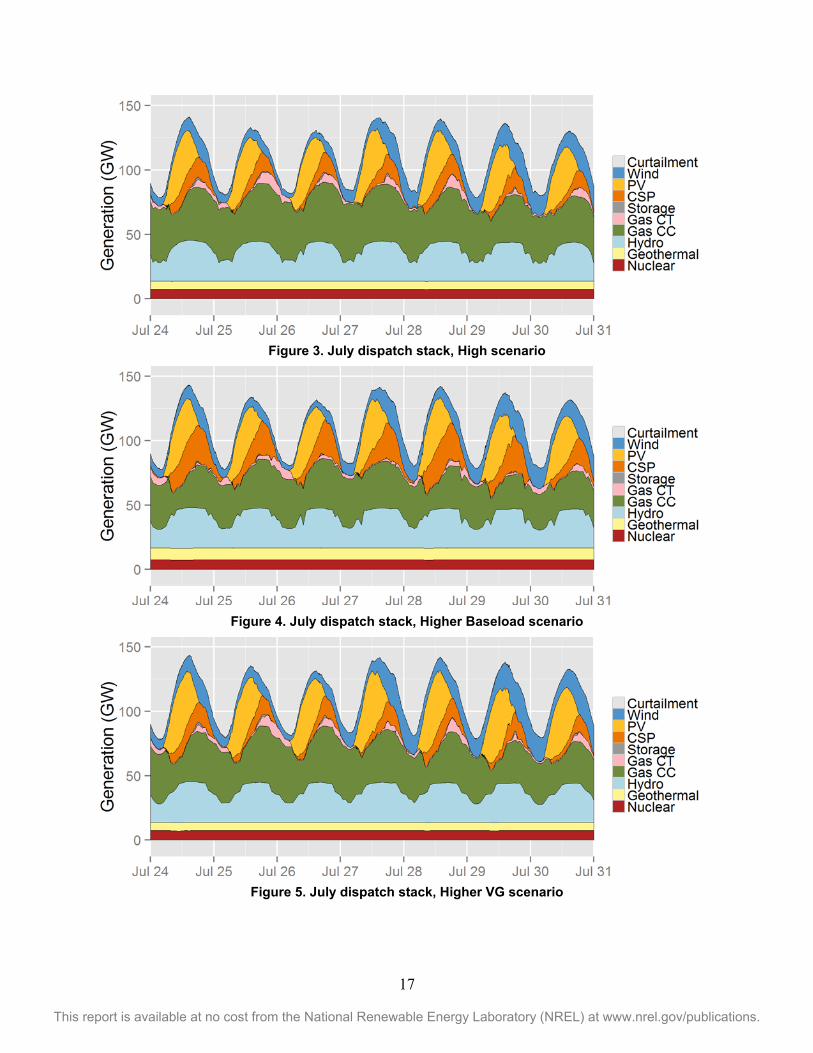
3.3 System Dispatch Figure 3 through Figure 5 show seven days of dispatch during July, a high-load period that shows no curtailment in any of the cases. The dispatch of the system was similar in all of the cases. Nuclear and geothermal provided baseload power, while the wind, PV, and CSP reduced the peak power requirement by approximately 50 GW each day. The remaining flexibility was provided by hydropower ramping between overnight and daytime hours and gas combustion turbines (CTs) coming online to provide power at sunset. With high PV penetration, sunset was consistently when the gas fleet was needed to provide the most power. During summer, the diurnal shape of the dispatch was very consistent, and most generator types did a single period of ramping up and down each day.

17


Figure 3. July dispatch stack, High scenario

Figure 4. July dispatch stack, Higher Baseload scenario

Figure 5. July dispatch stack, Higher VG scenario

18


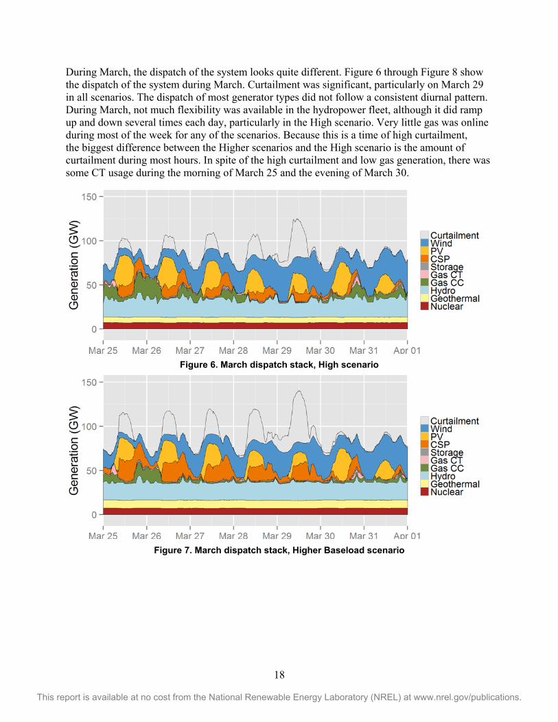
During March, the dispatch of the system looks quite different. Figure 6 through Figure 8 show the dispatch of the system during March. Curtailment was significant, particularly on March 29 in all scenarios. The dispatch of most generator types did not follow a consistent diurnal pattern. During March, not much flexibility was available in the hydropower fleet, although it did ramp up and down several times each day, particularly in the High scenario. Very little gas was online during most of the week for any of the scenarios. Because this is a time of high curtailment, the biggest difference between the Higher scenarios and the High scenario is the amount of curtailment during most hours. In spite of the high curtailment and low gas generation, there was some CT usage during the morning of March 25 and the evening of March 30.

Figure 6. March dispatch stack, High scenario

Figure 7. March dispatch stack, Higher Baseload scenario

19


Figure 8. March dispatch stack, Higher VG scenario

Reserves are relatively simple for the system to procure in all of the cases. In most regions (and all scenarios), reserves had no additional cost for more than three-fourths of the hours. At very high instantaneous penetrations, wind and solar curtailment can provide reserves to the system. At moderate levels of penetration, enough gas and other generation were online to provide reserves. Table 8 shows which technologies provided contingency and regulating reserves to the system on average for the three scenarios. In all cases, the majority of the reserves were provided by renewables (hydropower, CSP, and curtailed wind and PV). The remaining reserves were nearly equally split between storage and thermal generation.

Table 8. Fraction of Reserves Procured by Technology Type

Type High Higher Baseload Higher VG

Hydropower 32% 32% 32%

Storage 19% 18% 18%

Gas CC 13% 9% 11%

CSP 12% 16% 12%

Wind and PV 11% 13% 14%

Other thermal 8% 7% 7%

Gas CT 3% 3% 4%

Demand response 2% 2% 2%

20


Similar resources provided flexibility reserves as well. These reserves were released in the real-time dispatch and allowed to provide energy or other ancillary services. The amount of reserves required were based on the methodology described in Section 2 is shown in Table 9. The flexibility reserve requirement was slightly higher than the contingency requirement, which was 3% of load in most balancing authorities in the model. The regulation reserve requirement was approximately 1.6% of load while the flexibility reserve requirement was approximately 3.4% of load.

Table 9. Average Annual Reserve Requirements

Type Reserve Requirement (MW)

Regulation 1,450

Contingency 2,760

Flexibility 3,090

3.4 Curtailment and Prices This section analyzes in detail the VG curtailment seen during the sample weeks in Section 3.3. Figure 9 through Figure 11 show a duration curve of curtailment in the scenarios. Although the plots are labeled with hours in the x-axis for clarity, this is a result of modeling with five-minute resolution. In the High scenario, curtailment peaked at 56 GW throughout the Western Interconnection. In the Higher Baseline and Higher VG, curtailment peaked at 71 GW and 73 GW, respectively. The shape of the curtailment was similar in all scenarios, with the majority of the curtailment occurring during a small number of hours, similar to mid-day on March 29 in the dispatch stacks in Section 3.3. Curtailment followed a similar pattern in each region of the scenarios, with the larger curtailments generally happening in regions with more installed VG capacity.

21


Figure 9. Curtailment duration curve, High scenario

Figure 10. Curtailment duration curve, Higher Baseload scenario

22


Figure 11. Curtailment duration curve, Higher VG scenario

Analyzing the curtailment can help understand potential solutions to reduce curtailment. For these scenarios, the transmission expansion described in Section 2.2 has been included. Because the majority of the curtailment occurs during a small number of hours, potential solutions would have to be able to handle a significant amount of renewable power during those hours. Figure 12 shows the average price duration curve for the regions of the study. In each region, there are close to 2,000 hours of zero price, and because these hours partially coincide, there are approximately 1,800 hours of zero price interconnection-wide. Curtailment during these hours would not be mitigated even if there were no transmission constraints.

Table 10 shows the percentage of curtailment that occurs during hours where the price is zero throughout the interconnection. Depending on the scenario, 66%–80% of curtailment occurs during these hours, and no amount of transmission expansion (unless it connects with other interconnections) will relieve this curtailment.

23


Figure 12. Price duration curve, High scenario

Table 10. Curtailment during Zero-Price Hours throughout the Interconnection

Scenario Hours During which Average Price in Western Interconnection is Near $0/MWh

Percentage of Curtailment that Occurs During Zero-Price Hours

High 1,780 hours 66%

Higher Baseload 2,640 hours 75%

Higher VG 2,610 hours 80%

24


Figure 13 shows the diurnal pattern of the curtailment (averaged throughout the year) for the scenarios. It followed approximately the same shape as the solar PV profiles. Although the curtailment appeared to be primarily caused by PV, there was still a significant amount of wind online during times of curtailment. More than half of the curtailment was assigned to wind (based on the amount of power coming from wind and PV during times of curtailment), although there was more than twice as much wind generation as PV generation in all scenarios. Successful curtailment reduction technology would shift demand from evening (or possibly morning) hours to mid-day. Storage or demand response could play this role, and to this end, a simple storage sensitivity was analyzed (see Section 4.3). The ideal curtailment reduction would be able to shift the load by at least 6 hours, to increase the load between hours 9 and 15 and reduce the load outside those hours. Although the added storage devices had 12 hours of storage, 6 hours of storage was enough to achieve most of the curtailment benefit.

Figure 13. Diurnal curtailment in all scenarios

25


Figure 14 shows the monthly distribution of curtailment. Approximately two-thirds of curtailment occurred during January through May in all scenarios, and almost half occurred during March, April, and May. The monthly curtailment shapes can help identify when the curtailment is occurring seasonally, and they can identify whether there are possible seasonal solutions to help with curtailment. Although short-term (6–12 hour) storage can help with the diurnal shape, other solutions may help with the seasonal nature. Any storage for this purpose would have to have very large energy reservoirs. However, maintenance scheduling could play a role in seasonal curtailment reduction, and shutting down nuclear or other baseload generation seasonally (for longer than standard maintenance periods) could also reduce curtailment.

Figure 14. Monthly curtailment in all scenarios

26


3.5 Penetration of Variable Generation This section examines VG penetrations throughout the interconnection. The metric is the fraction of generation at a given five-minute interval that comes from VG. Figure 15 shows a time series for the VG penetration for the entire year. As loads get higher during the summer, VG penetrations get lower. The highest VG penetrations occur during the fall, as hydropower is lower in the fall compared to the spring. The peak VG penetrations were limited by the constraints on the system, not by VG capacity. For example, there was enough wind and PV on March 29 to supply all load on the system, but the hydro, geothermal, and nuclear generation were dispatched prior to VG. Nuclear is considered must-run generation in the modeling, and hydro and geothermal resources have constraints that prevent shutdown in the model (and in reality). There was also a very small amount of gas online during those hours.

Figure 15. Time series of fraction of generation from VG sources, High scenario

27


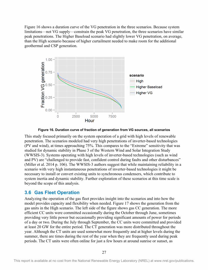
Figure 16 shows a duration curve of the VG penetration in the three scenarios. Because system limitations—not VG supply—constrain the peak VG penetration, the three scenarios have similar peak penetrations. The Higher Baseload scenario had slightly lower VG penetration, on average, than the High scenario because of higher curtailment needed to make room for the additional geothermal and CSP generation.

Figure 16. Duration curve of fraction of generation from VG sources, all scenarios

This study focused primarily on the system operation of a grid with high levels of renewable penetration. The scenarios modeled had very high penetrations of inverter-based technologies (PV and wind), at times approaching 75%. This compares to the “Extreme” sensitivity that was studied for dynamic stability in Phase 3 of the Western Wind and Solar Integration Study (WWSIS-3). Systems operating with high levels of inverter-based technologies (such as wind and PV) are “challenged to provide fast, confident control during faults and other disturbances” (Miller et al. 2014 p. 106). The WWSIS-3 authors suggest that while maintaining reliability in a scenario with very high instantaneous penetrations of inverter-based technologies it might be necessary to install or convert existing units to synchronous condensers, which contribute to system inertia and dynamic stability. Further exploration of these scenarios at this time scale is beyond the scope of this analysis.

3.6 Gas Fleet Operation Analyzing the operation of the gas fleet provides insight into the scenarios and into how the model provides capacity and flexibility when needed. Figure 17 shows the generation from the gas units in the High scenario. The left side of the figure shows gas CC generation. The more efficient CC units were committed occasionally during the October through June, sometimes providing very little power but occasionally providing significant amounts of power for periods of a day or two. During the July through September, the CC units were committed and provided at least 20 GW for the entire period. The CT generation was more distributed throughout the year. Although the CT units are used somewhat more frequently and at higher levels during the summer, there are times during the rest of the year when they are frequently used during peak periods. The CT units were often online for just a few hours at around sunrise or sunset, as

28


shown in Section 3.3. Often the peak in net load at sunset was a short occurrence, with load declining later in the evening and the CTs shutting down.

Figure 17. Time series of gas generation in the High scenario

In the Higher Baseload and Higher VG scenarios, the time series of dispatch was similar to the High scenario, with a little less use of the gas CCs. Figure 18 shows a duration curve of the three scenarios. As the usage of CTs is primarily for flexibility during brief periods, the usage of these is not significantly impacted between the scenarios. Some CC generation was displaced in the Higher Scenarios, with more displaced in the Higher Baseload scenario due to the VG curtailments in the Higher VG scenario.

Figure 18. Duration curve of gas generation in all three scenarios

29


3.7 Transmission Utilization As has been seen in previous studies (e.g., RE Futures [Mai et al. 2012]), the transmission system is mostly used bi-directionally. In most cases, power is not simply transmitted in one direction at all times to ship power from one renewable resource location to load. Figure 19 shows the annual time series of transmission along six key interfaces in the Western Interconnection. Along most of these interfaces, the lines may be congested in opposite directions in the same day. Bi-directional flow means that different types of power (e.g., PV, wind) flow to different regions depending on the output and loads at different hours. It also enables the regions to balance load using the least-expensive possible generation. For example, this can include a region with high PV penetration shipping power out during the day and importing power from an adjoining region with high wind penetration during the evening. These changes in direction often follow a diurnal cycle along with the PV output and load.

The interface between northern and southern California is commonly congested today, but with the new PV generation in southern California and new transmission going into northern California in the scenarios, this interface was rarely congested in our results.

Figure 19. Time series of transmission along selected interfaces, High scenario

30


Figure 20 shows a duration curve of the same transmission flows. Congested flows with the interfaces at the flow limits show up as flat lines in the top left or bottom right corners of the plot. There is a wide variety of flows across all these interfaces, although several of them flow the same direction most of the time (e.g., Los Angeles Department of Water and Power imports from the Northwest and the Northwest imports from Montana). Table 11 shows the transmission utilization between the scenarios. The time series and duration curves were very similar for the three scenarios, and the transmission utilization was slightly higher in the cases with higher renewable generation.

Figure 20. Duration curve of transmission along selected interfaces, High scenario

Table 11. Transmission Utilization in the Three Scenarios

Scenario Transmission Utilization

High 0.44

Higher Baseload 0.46

Higher VG 0.46

Transmission utilization is defined as the fraction of available transmission capacity that is used, averaged throughout the year.

31


3.8 Production Costs Previous RE Futures reports (Mai et al. 2012 and 2014) performed detailed cost analyses, including operational and capital costs. This study focused on operational impacts of high renewable penetrations, and Table 12 shows the sum of these costs from the sub-hourly modeling. The vast majority of the operational costs were for fuel, while startup costs and variable operation and maintenance (VO&M) costs made up 2.4% and 4.9% of the total costs.

In the Higher Baseload case, total production cost was reduced by $1.5 billion due to the addition of 68 TWh of CSP and geothermal generation. This included a $50 million reduction in startup costs due to less reliance on gas generation. In the Higher VG case, total production cost was reduced by $860 million due to the addition of 68 TWh of wind and solar PV. The production cost change was lower due to the additional curtailment in the Higher VG case compared to the Higher Baseload case. This included a $20 million increase in startup costs. A full capital cost analysis would help analyze the tradeoffs between capital costs and operational costs for VG, baseload renewables, storage, and other technologies. Although gas generation was displaced, the additional flexibility required by the incremental VG caused the startup costs to increase by 8% more than the High scenario.

Because most of the generation comes from sources with negligible operating costs, the production cost was less than $10/MWh in each scenario. This was much lower than the cost of natural gas combined cycle generation, which is approximately $35/MWh using the assumed gas price of $4.60/mmBtu. For reference, the production cost for the Western Interconnection with 0%, 11%, and 33% wind and solar penetrations from the WWSIS-2 study was approximately $18 billion, $15 billion, and $11 billion (respectively). Although the gas price was the same, several differences in the model made the generation fleet not directly comparable (e.g., all coal generation was retired for this study).

Table 12. Total Production Costs for the Three Scenarios

Scenario Fuel Cost (million $)

VO&M Cost (million $)

Start Cost (million $)

Total Production Cost (million $)

Production Cost per MWh ($/MWh)

High 8,657 465 225 9,348 9.6

Higher Baseload 7,252 415 178 7,844 8.0

Higher VG 7,809 432 244 8,485 8.7

32


4 Sensitivity Results This section describes the results of the sensitivity cases that explored the impact of generator flexibility, transmission interface efficiency, and storage on the High scenario. The impact of generator flexibility was tested in the High LoFlex case (Section 4.1) by requiring that gas CC generators are committed in a day-ahead (DA) market and have minimum run times of 24 hours. This sensitivity could also represent a case where markets are not flexible enough to fully utilize the capabilities of the generators. For example, an inflexible market may commit units with four-hour start times in a DA market. The impacts of transmission flexibility were tested in the High LoFlex no DA and no DA/RT cases (Section 4.2). These cases were comparable to the High LoFlex case, but very high hurdle rates ($40/MWh) were added to the DA market (in the no DA case) and to both the DA and the RT markets in the no DA/RT case. These hurdle rates create friction between markets and cause regions to commit primarily local generators and avoid inter-regional transmission except in cases where the electricity prices differ by more than $40/MWh (e.g., local CC generation will be committed instead of importing free electricity). This case is extreme case and unlikely to occur throughout the interconnection, but it provides information on how much benefit could come from increasing the ability to transfer power efficiently between regions. The impacts of storage were simulated in a case that adds a large amount of storage (10 GW) to the three regions with highest curtailment (Section 4.3). Table 13 shows the changes to the assumptions for each sensitivity.

Table 13. Assumptions for the Sensitivities in this Study

Region DA or 4HA Commitment of Gas CC Generators

Min. Run Time for CC Generators

DA/4HA Hurdle Rates

RT Hurdle Rates

Additional Storage Generation

High 4HA 8 hours 0 0 0

High LoFlex DA 24 hours 0 0 0

High LoFlex no DA DA 24 hours $40/MWh 0 0

High LoFlex no DA/RT DA 8 hours $40/MWh $40/MWh 0

High Storage 4HA 8 hours 0 0 10 GW

While the remainder of this section contains tables and figures that apply to all of the sensitivities, Sections 4.1 through 4.3 describe the results of each sensitivity in detail. Figure 21 shows the annual generation by type in each of the sensitivities. The generation fleet was the same in each sensitivity, with the exception of some of the properties of the gas CC generators in the High LoFlex case and the additional storage in the High Storage case. Table 14 shows the annual production cost in each sensitivity, which is useful for understanding the value of different types of flexibility. Table 15 shows how curtailment was affected in each of the sensitivities, and how that affects the renewable penetration. Figure 22 presents a duration curve of the gas fleet in the different sensitivities to show how the gas fleet responded to the different conditions and assumptions.

33


Figure 21. Generation by type in the sensitivities, after curtailment

Table 14. Total Production Costs for the Sensitivities

Scenario Fuel Cost (Million $)

VOM Cost (Million $)

Start Cost (Million $)

Total Production Cost (Million $)

High 8,657 465 225 9,348

High LoFlex 8,991 466 243 9,700

High LoFlex no DA 9,748 492 171 10,410

High LoFlex no DA/RT 11,349 546 171 12,066

High Storage 8,260 458 130 8,848

Table 15. Penetration of Renewables, VG, and Curtailment for the Three Scenarios

Scenario Actual Penetration of VG

Actual Penetration of Renewables

Curtailment as Fraction of Possible VG

Curtailment as Fraction of Possible Renewables

High 41.3% 81.5% 12.4% 6.7%

High LoFlex 41.0% 81.0% 12.0% 6.5%

High LoFlex no DA 39.0% 78.4% 16.2% 8.9%

High LoFlex no DA/RT 32.4% 71.7% 30.6% 16.8%

High Storage 42.2% 83.0% 9.4% 5.1%

34


Figure 22. Duration curve of gas generation in the sensitivities

4.1 Flexibility of the Thermal Fleet The High LoFlex explored the impact of less flexibility in the thermal fleet. This could represent either a case where the coal fleet does not experience significant retirements or a case in which institutional constraints (e.g., bilateral contracts, market structures that do not include any intra-day re-commitments) reduce the ability of the thermal fleet to be able to provide flexibility that is technically possible.

The High LoFlex case assumed that all gas CC generators must be committed during a day-ahead unit commitment (instead of 4HA commitment), requiring the use of forecasts with longer lead times and less accuracy. It also assumed the gas CC units have minimum run times of 24 hours. This makes the CC units similar to a typical coal unit, although we left all costs (fuel costs, VO&M, and startup costs) identical to the other scenarios so that the results from the High LoFlex case could be compared directly with the High case. This case gives us insights into the potential impacts of having a less flexible thermal fleet.

Figure 21 shows that the annual dispatch of the system was quite similar in the High LoFlex and High cases. The additional constraints on the gas generators caused the system to use less gas CC generation and more gas CT generation. This is probably due to the higher forecast error in the DA market, and the system calls upon CT generation during times when the CC generation is under-committed. Figure 23 shows the sample week of dispatch in March, and the only noticeable difference between the High LoFlex and High cases is the addition of gas CT generation during morning and evening of days (it replaces gas CC generation). This same pattern is shown in the total annual numbers. Figure 22 shows another way of viewing this change, where the gas CT generation operated at higher levels for more hours of the year.

The difference between the High and High LoFlex cases was more noticeable in the production costs in Table 14. The reduction in flexibility cost the system $350 million, which represents a 3.8% increase in production costs, or $0.48 per MWh delivered. Approximately half of this

35


production cost difference is explained by switching from gas CC to gas CT generation; the other half is due to less efficient operation of the gas CC fleet (e.g., operation at part-load).

The High LoFlex case shows slightly lower curtailment than the High case (see Table 15); this is because the model chooses to back down CSP dispatch slightly. This reduction of CSP output was not counted towards curtailment in Table 14 because it is difficult to classify for CSP, which has six hours of thermal storage. However, if counted, it would eliminate the difference in curtailment between the High (6.7%) and the High LoFlex (6.5%) cases.

Figure 23. March dispatch stack, High LoFlex case

4.2 Flexibility from Interchange This section explores the impact of reducing the ability of the model to efficiently exchange power between regions in the DA and RT markets. The inefficiency and friction are introduced by adding hurdle rates to the model. Hurdle rates add to the optimization cost in the PLEXOS model for every MWh that is transmitted over a given path. For these runs, to encourage regions to supply their own electricity when possible, we added very high ($40/MWh) hurdle rates. The hurdle rates were added in only the DA market for the no DA case and in both the DA and RT markets for the no DA/RT case. When added only in the DA market, the hurdle rates imitate a system where regions try to self-commit their generation but there is efficient real-time trading for energy imbalances. Currently, there is not a DA or RT market between all of the balancing authorities in the Western United States. The California Independent System Operator (CAISO) is the largest DA market, while there is a new energy imbalance market among CAISO, PacifiCorp, NV Energy, Arizona Public Service, and Puget Sound Energy in the West that allows for real-time trading within a market framework (California ISO 2015). There are varying amounts of friction between other balancing authorities in the West.

The framework for comparison of these cases is the High LoFlex sensitivity because its dispatch system and day-ahead market provided a clearer platform for comparison of interchange flexibility than the 4HA market (which would provide more flexibility than what currently exists in some regions) that is used the High scenario. These cases explored a situation where there is a

36


combination of inefficiencies in the dispatch of different regions due to inefficiencies between markets and inability to access all potential generator flexibility.

Figure 21 shows the impacts of reducing transmission flexibility on annual generation from each type of generator. Because regions are self-supplying, the gas CC commitment and generation went up significantly in both cases. This was primarily at the cost of increased curtailment, although the additional gas CC commitment does lead to a reduced usage of gas CT peaker generation. The overcommitment of gas CC generation is also noticeable in Figure 24 and Figure 25, when gas CC generation is committed even though it is unnecessary and curtailment is high. For example, on March 28 and March 29, there were two days of almost continuous curtailment while gas CC generation simultaneously generated 5–15 GW. This did not happen in the High LoFlex case because the power was efficiently shipped from areas with excess renewable generation to areas with load.

Figure 22 shows that even in the no DA case, gas CC generation never went below 5 GW, while all of the cases that included efficient exchange of power had gas CC generation going down to approximately 1 GW for many hours of the year. The no DA/RT case rarely had gas CC generation below 10 GW.

Figure 24. March dispatch stack, High LoFlex no DA case

Figure 25. March dispatch stack, High LoFlex no DA/RT case

37


The production cost changes due to transmission friction are shown in Table 14. The hurdle rate costs are included in the PLEXOS optimization, but they are not included in the production costs in Table 14. The increase in costs was due only to the inefficient dispatch because of the friction from the hurdle rates. The lack of DA coordination increased production costs by $700 million compared to the High LoFlex case, which is $0.96/MWh delivered and a 7.3% increase in total production costs. The lack of DA and RT coordination cost the model $2.4 billion more than the High LoFlex case, which is $3.2/MWh delivered and a 24% increase in production costs. These are extreme cases, and the $40/MWh caused the model to generate with gas CCs prior to importing free power. However, it demonstrates the impact of market friction is significant enough to cause changes in unit commitment patterns.

Table 15 shows that transmission friction has a significant impact on curtailment and renewable penetrations, also. Curtailment went from 7% in the High LoFlex case to 9% in the case with no DA coordination, to 17% in the case with no DA or RT coordination. This is because gas CC units operated in regions adjacent to other regions that were curtailing electricity. This result shows that reaching renewable penetrations of 80% and higher could be quite difficult without either balancing areas coordinating transmission or some other mitigating mechanism (e.g., more storage or only local renewables) in place.

Table 16 shows the contrast in transmission utilization between the High LoFlex and the two cases with friction between regions. In the LoFlex no DA case, transmission utilization was reduced to 0.37 (from 0.44), but the model continued to transfer a significant amount of power after the overcommitment of the gas CC generation. In the LoFlex no DA/RT case, transmission utilization was reduced to 0.09, as renewables were curtailed while gas CC generation in neighboring regions ran at its full capacity. There was not enough incentive in the LoFlex no DA/RT case even to turn down the overcommitted gas CC generation to reduce curtailment in adjacent regions. Flow duration curves for the six selected interfaces in these sensitivities are shown in the appendix.

Table 16. Total Production Costs for the Sensitivities

Scenario Transmission Utilization

High LoFlex 0.44

High LoFlex no DA 0.37

High LoFlex no DA/RT 0.09

Transmission utilization is defined as the fraction of available transmission capacity that is used, averaged throughout the year.

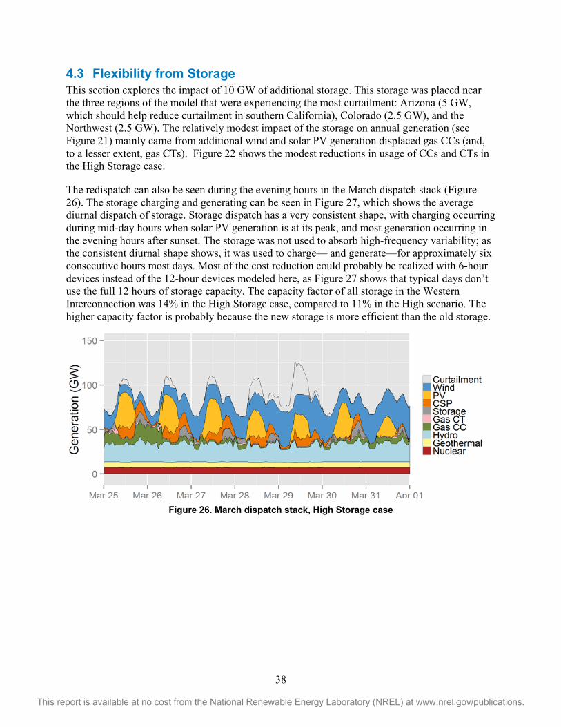
38


4.3 Flexibility from Storage This section explores the impact of 10 GW of additional storage. This storage was placed near the three regions of the model that were experiencing the most curtailment: Arizona (5 GW, which should help reduce curtailment in southern California), Colorado (2.5 GW), and the Northwest (2.5 GW). The relatively modest impact of the storage on annual generation (see Figure 21) mainly came from additional wind and solar PV generation displaced gas CCs (and, to a lesser extent, gas CTs). Figure 22 shows the modest reductions in usage of CCs and CTs in the High Storage case.

The redispatch can also be seen during the evening hours in the March dispatch stack (Figure 26). The storage charging and generating can be seen in Figure 27, which shows the average diurnal dispatch of storage. Storage dispatch has a very consistent shape, with charging occurring during mid-day hours when solar PV generation is at its peak, and most generation occurring in the evening hours after sunset. The storage was not used to absorb high-frequency variability; as the consistent diurnal shape shows, it was used to charge— and generate—for approximately six consecutive hours most days. Most of the cost reduction could probably be realized with 6-hour devices instead of the 12-hour devices modeled here, as Figure 27 shows that typical days don’t use the full 12 hours of storage capacity. The capacity factor of all storage in the Western Interconnection was 14% in the High Storage case, compared to 11% in the High scenario. The higher capacity factor is probably because the new storage is more efficient than the old storage.

Figure 26. March dispatch stack, High Storage case

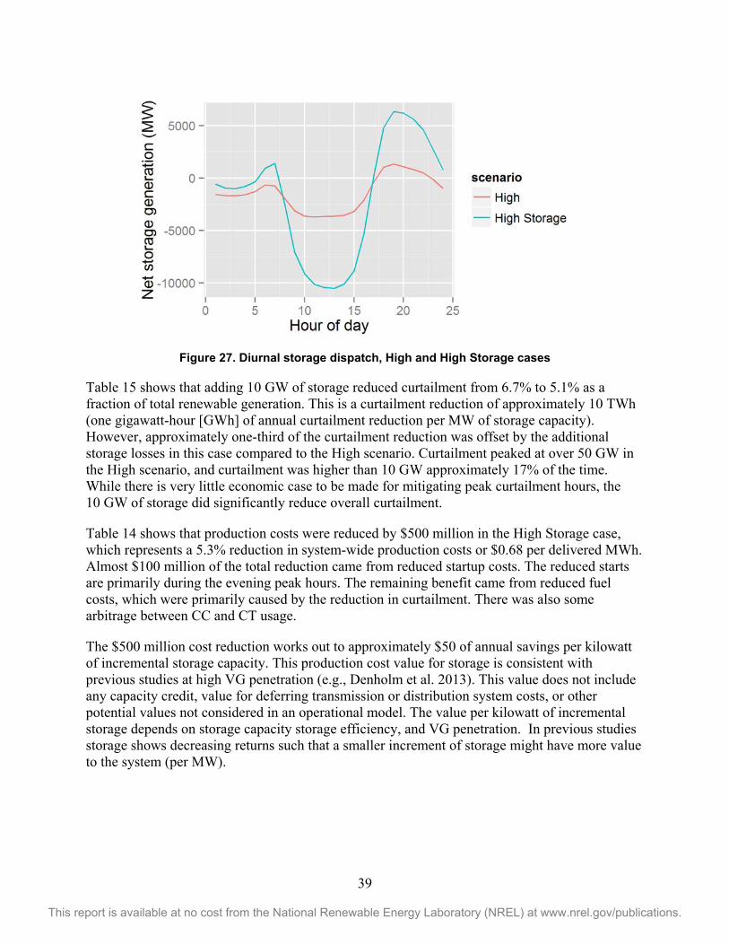
39


Figure 27. Diurnal storage dispatch, High and High Storage cases

Table 15 shows that adding 10 GW of storage reduced curtailment from 6.7% to 5.1% as a fraction of total renewable generation. This is a curtailment reduction of approximately 10 TWh (one gigawatt-hour [GWh] of annual curtailment reduction per MW of storage capacity). However, approximately one-third of the curtailment reduction was offset by the additional storage losses in this case compared to the High scenario. Curtailment peaked at over 50 GW in the High scenario, and curtailment was higher than 10 GW approximately 17% of the time. While there is very little economic case to be made for mitigating peak curtailment hours, the 10 GW of storage did significantly reduce overall curtailment.

Table 14 shows that production costs were reduced by $500 million in the High Storage case, which represents a 5.3% reduction in system-wide production costs or $0.68 per delivered MWh. Almost $100 million of the total reduction came from reduced startup costs. The reduced starts are primarily during the evening peak hours. The remaining benefit came from reduced fuel costs, which were primarily caused by the reduction in curtailment. There was also some arbitrage between CC and CT usage.

The $500 million cost reduction works out to approximately $50 of annual savings per kilowatt of incremental storage capacity. This production cost value for storage is consistent with previous studies at high VG penetration (e.g., Denholm et al. 2013). This value does not include any capacity credit, value for deferring transmission or distribution system costs, or other potential values not considered in an operational model. The value per kilowatt of incremental storage depends on storage capacity storage efficiency, and VG penetration. In previous studies storage shows decreasing returns such that a smaller increment of storage might have more value to the system (per MW).

40


5 Conclusions In the RE Futures study (Mai et al. 2012), the production cost modeling of the operation of the grid was performed with an hourly time step. Operation of the simulated system was possible at the hourly time step, and curtailment was between 8% and 10% of wind, solar, and hydropower generation for scenarios that were close to 80%. RE Futures did not address any impacts that occur in a sub-hourly time scale. This report attempts to address impacts that may occur in the sub-hourly time frame by including real-time dispatch of the system with five-minute time resolution. Our work focused on the Western Interconnection, and it used methodologies and data sets that have been reviewed by stakeholders for several previous studies. Using more advanced modeling techniques such as improved transmission modeling, five-minute time resolution, and mixed integer programming optimization, we reinforce findings from RE Futures and show the system can be balanced at a 5-minute level. Other important conclusions from this work are:

• Curtailment is consistent with prior RE Futures study results and reliability metrics that can be obtained from sub-hourly unit commitment and dispatch modeling (e.g., unserved load, unserved reserves, planning reserve margin for the net load) did not indicate any reliability problems.

• Curtailment ranges from 5% to 11% for the 82%–88% penetration cases, assuming no significant friction exists between markets. This is consistent with the original RE Futures study (Mai et al. 2012), which reported 8%–10% curtailment for a scenario that was approximately 80% penetration.

• Although curtailment is not greatly impacted by modest changes to generator fleet flexibility, reducing the flexibility of the gas CC fleet cost the system $350 million ($0.48 per delivered MWh).

• Simulation of friction between markets leads to increases in costs and curtailment. The lack of coordinated day-ahead planning could cost the simulated system over $700 million ($0.96/MWh) and increased curtailment from 7% to 9%.

• In our results, transmission helps alleviate curtailment, at high penetrations of renewables and VG. However, 66%–80% of the curtailment occurs when curtailment is happening throughout the interconnection and more transmission cannot mitigate this curtailment.

• Storage can reduce curtailment by one GWh per MW of storage capacity, for a value of approximately $50/kW of storage capacity (or $0.68 per delivered MWh). Ten GW of storage could reduce curtailment from 7% of possible renewable generation to 5%.

• Marginal prices may be near zero a significant fraction of the time (20%–30% of the time in these scenarios) if annual renewable penetration is above 80%. Capacity factors at thermal power plants go down in the cases we analyzed. These changes reduce financial returns on investment in generation if markets are based on marginal energy prices alone. Other types of markets (e.g., capacity markets, more ancillary service markets, renewable energy markets) may be needed to provide financial incentives to ensure sufficient capacity exists on the grid in a high renewables future.

41


• Our scenarios and sensitivities are not optimized. Other configurations of resources (including enabling technologies, such as storage and demand response) may be optimal for reliability, curtailment mitigation, or both. Other practices, such as additional transmission connecting the Western Interconnection with the Eastern Interconnection or the Texas Interconnection may also be beneficial, but they were not studied here.

• Future work (as described in WWSIS-3) will need to be done to ensure that scenarios like those used in this study can be operated reliably during contingencies and transient events. System upgrades, such as synchronous condensers and shunt capacitors may be necessary to ensure transient stability.

42


References 3TIER. 2010. Development of Regional Wind Resource and Wind Plant Output Datasets, NREL/SR-550-47676, Prepared by 3TIER for the National Renewable Energy Laboratory. Golden, CO: National Renewable Energy Laboratory. http://www.nrel.gov/docs/fy10osti/47676.pdf.

California ISO. 2015. “Energy Imbalance Market Overview.” Accessed July 2, 2015. http://www.caiso.com/informed/Pages/EIMOverview/Default.aspx.

Denholm, Paul, Jennie Jorgenson, Marissa Hummon, Thomas Jenkin, David Palchak, Brendan Kirby, Ookie Ma, and Mark O’Malley. 2013. The Value of Energy Storage for Grid Applications. NREL/TP-6A20-58465. Golden, CO: National Renewable Energy Laboratory. http://www.nrel.gov/docs/fy13osti/58465.pdf.

E3 (Energy and Environmental Economics). 2014. Investigating a Higher Renewables Portfolio Standard in California. San Francisco: : Energy and Environmental Economics.. https://ethree.com/documents/E3_Final_RPS_Report_2014 _01_06_with_appendices.pdf .

GE Energy. 2010. Western Wind and Solar Integration Study. NREL/SR-550-47434. Prepared by GE Energy for the National Renewable Energy Laboratory. Golden, CO: National Renewable Energy Laboratory. http://www.nrel.gov/docs/fy10osti/47434.pdf.

GE Energy. 2014a. PJM Renewable Integration Study: Executive Summary Report. Prepared by GE Energy for PJM Interconnection, LLC. Schenectady, NY: GE Energy. http://www.pjm.com/ ~/media/committees-groups/subcommittees/irs/postings/pris-executive-summary.ashx.

GE Energy. 2014b. Minnesota Renewable Energy Integration and Transmission Study Final Report. Prepared by GE Energy for the Minnesota Utilities and Transmission Companies and the Minnesota Department of Commerce. Schenectady, NY: GE Energy. http://www.minnelectrans.com/documents/MRITS-report.pdf.

Guo, Tao. 2014. Renewable Generation Integration Study by PLEXOS. Sacramento, CA: Energy Exemplar. http://energyexemplar.com/wp-content/uploads/2014/09/Renewable-Generation-Integration.pdf.

Hummon, Marissa, Eduardo Ibanez, Gregory Brinkman, and Debra Lew. 2012. Sub-Hour Solar Data for Power System Modeling From Static Spatial Variability Analysis. NREL/CP-6A20-56204. Golden, CO: National Renewable Energy Laboratory. http://www.nrel.gov/docs/fy13osti/56204.pdf.

Lew D., G. Brinkman, E. Ibanez, A. Florita, M. Heaney, B.-M. Hodge, M. Hummon, G. Stark, J. King, S.A. Lefton, N. Kumar, D. Agan, G. Jordan, and S. Venkataraman. 2013. The Western Wind and Solar Integration Study Phase 2. NREL/TP-5500-55588. Golden, CO: National Renewable Energy Laboratory. http://www.nrel.gov/docs/fy13osti/55588.pdf.

http://www.nrel.gov/docs/fy10osti/47676.pdf

http://www.caiso.com/informed/Pages/EIMOverview/Default.aspx


https://ethree.com/documents/E3_Final_RPS_Report_2014_01_06_with_appendices.pdf

https://ethree.com/documents/E3_Final_RPS_Report_2014_01_06_with_appendices.pdf


http://www.pjm.com/~/media/committees-groups/subcommittees/irs/postings/pris-executive-summary.ashx

http://www.pjm.com/~/media/committees-groups/subcommittees/irs/postings/pris-executive-summary.ashx

http://www.minnelectrans.com/documents/MRITS-report.pdf

http://energyexemplar.com/wp-content/uploads/2014/09/Renewable-Generation-Integration.pdf

http://energyexemplar.com/wp-content/uploads/2014/09/Renewable-Generation-Integration.pdf



43


Mai, T., R. Wiser, D. Sandor, G. Brinkman, G. Heath, P. Denholm, D.J. Hostick, N. Darghouth, A. Schlosser, K. Strzepek. 2012. Exploration of High-Penetration Renewable Electricity Futures. Vol. 1 of Renewable Electricity Futures Study. NREL/TP-6A20-52409-1. Golden, CO: National Renewable Energy Laboratory. http://www.nrel.gov/analysis/re_futures/.

Mai, Trieu, David Mulcahy, M. Maureen Hand, and Samuel F. Baldwin. 2014. “Envisioning a Renewable Electricity Future for the United States,” Energy 65: 374–386.

Milligan, M., K. Clark, J. King, B. Kirby, T. Guo, G. Liu. 2012. Examination of Potential Benefits of an Energy Imbalance Market in the Western Interconnection. NREL/TP-5500-57115. Golden, CO: National Renewable Energy Laboratory. http://www.nrel.gov/docs/fy13osti/57115.pdf.

Miller, N., M. Shao, S. Pajic, and R. D’Aquila. 2014. Western Wind and Solar Integration Study Phase 3: Frequency Response and Transient Stability. NREL/SR-5D00-62906. Prepared by GE Energy for the National Renewable Energy Laboratory. Golden, CO: National Renewable Energy Laboratory. http://www.nrel.gov/docs/fy15osti/62906.pdf.

WECC (Western Electricity Coordinating Council). 2011. 10-Year Regional Transmission Plan 2020 Study Report: TEPPC 2010 Study Program. Salt Lake City: Western Electricity Coordinating Council. https://www.wecc.biz/Reliability/2011Plan_2020%20Study %20Report.pdf.

http://www.nrel.gov/analysis/re_futures/



https://www.wecc.biz/Reliability/2011Plan_2020%20Study%20Report.pdf

https://www.wecc.biz/Reliability/2011Plan_2020%20Study%20Report.pdf

44


Appendix Figure A-1 shows the transmission capacity between regions prior to the transmission buildout for this study. Figures A-2 through A-4 show the duration curve of transmission flows across selected interfaces in the High LoFlex, High LoFlex no DA, and High LoFlex no DA/RT scenarios.

Figure A-1. Assumed transmission between “bubbles” in the Western Interconnection

(prior to transmission buildout for this study)

2000

325 4001800

3002200

4200

350775 400

1400100

360650

12722750 1920

2502858 664

3000 250

3883

37504785

2814 4685582

1600600

1952440

150

1168

PacificNorthw est

NorthernCalifornia

SF

SMUD

LADWP

San Diego

Southern California

NorthernNev ada

Idaho

Montana

Wy oming

Colorado

New Mex ico

Southern Nev ada

ArizonaIID

Utah

MAPP

45


Figure A-2. Duration curve of transmission along selected interfaces, High LoFlex scenario

Figure A-3. Duration curve of transmission along selected interfaces, High LoFlex no DA scenario

46


Figure A-4. Duration curve of transmission along selected interfaces, High LoFlex no DA/RT

scenario

Documents

Renewable Electricity Futures: Operational Analysis of the ... · Operational Analysis of the ... (ECCO International) for their help in reviewing the methods, ... March dispatch