Embed Size (px)
Citation preview

Rendering: Path Tracing Basics
Bernhard Kerbl
Research Division of Computer Graphics
Institute of Visual Computing & Human-Centered Technology
TU Wien, Austria
Disclaimer and Errata
The following slides make heavy use of mathematical manipulations and pseudo code snippets for demonstration purposes
It is quite easy to make mistakes when setting them up as slides
If you find any issues, please feel free to notify us!
The recorded version of this lecture will include an Errata section
Rendering – Path Tracing Basics 2

Today’s Goal
We combine the things we learned so far to make our first unbiased path tracer for diffuse materials:
Light Physics
Monte Carlo Integration
The Rendering Equation
The Path Tracing Algorithm
Different iterations and considerations for performance
Introduce a dedicated BSDF/BRDF material data structureRendering – Path Tracing Basics 3

BSDF/BRDF..?
Bidirectional Scattering Distribution Function (BSDF) accounts for the light transport properties of the hit material
Bidirectional Reflectance Distribution Function (BRDF) considers only the reflection of incoming light onto a surface
Only diffuse materials for now, more in Materials lecture
Rendering – Path Tracing Basics 4

Material Types
We usually distinguish three basic material typesPerfectly diffuse (light is scattered equally in/from all directions)Perfectly specular (light is reflected in/from exactly one direction)Glossy (mixture of the other two, specular highlights)
Rendering – Path Tracing Basics 5
𝑛
𝑟𝑣𝑣
𝑛
𝑣
𝑛
𝑣 𝑟𝑣
𝑥𝑥𝑥
Diffuse Specular Glossy

Material Types
Rendering – Path Tracing Basics 6
Diffuse
We usually distinguish three basic material typesPerfectly diffuse (light is scattered equally in/from all directions)Perfectly specular (light is reflected in/from exactly one direction)Glossy (mixture of the other two, specular highlights)

What you will need
A basic scene with objects, some of which emit light
An output image to store color information in
A camera model in the scene for which you can make rays
E.g., with this detailed description by Scratchapixel
A function to trace rays through your scene and find the closest hit
E.g., using the famous Möller-Trumbore algorithm
Additional information for each hit point (normal, material, object)
So you can detect if an object was a light source, or
Use surface normals for computations
…Rendering – Path Tracing Basics 7

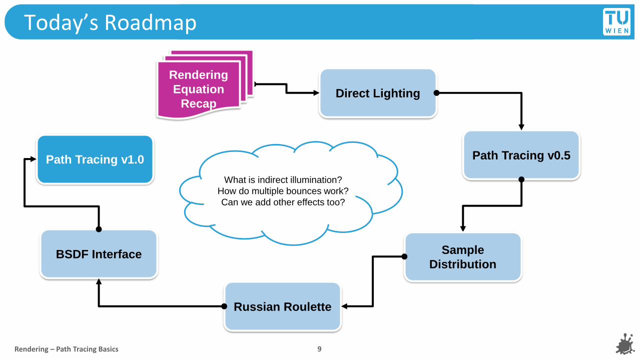
Today’s Roadmap
Rendering – Path Tracing Basics 8
What is indirect illumination?
How do multiple bounces work?
Can we add other effects too?
Direct Lighting
Path Tracing v1.0 Path Tracing v0.5
Rendering
Equation
Recap
BSDF Interface Sample
Distribution
Russian Roulette
Today’s Roadmap
Rendering – Path Tracing Basics 9
What is indirect illumination?
How do multiple bounces work?
Can we add other effects too?
Direct Lighting
Path Tracing v1.0 Path Tracing v0.5
Rendering
Equation
Recap
BSDF Interface Sample
Distribution
Russian Roulette

Recursive Rendering Equation, Recap
Rendering – Path Tracing Basics 10
Light going in direction v
Light from direction ω Solid angle
Material, modelled by the BRDF
Light emitted from x in direction v

Recursive Rendering Equation, Recap
Rendering – Path Tracing Basics 11
Light going in direction v
Evaluate light from direction ω recursively Solid angle
Material, modelled by the BRDF
Light emitted from x in direction v

Recursive Rendering Equation, Recap
To get the next bounce, we just evaluate this function recursively
Rendering – Path Tracing Basics 12

Today’s Roadmap
Rendering – Path Tracing Basics 13
What is indirect illumination?
How do multiple bounces work?
Can we add other effects too?
Direct Lighting
Path Tracing v1.0 Path Tracing v0.5
BSDF Interface Sample
Distribution
Russian Roulette
Rendering
Equation
Recap

We trace rays through a pixel that randomly bounce into the scene
Some will get lucky and hit light sources at first or second hit point!
Direct Lighting with the Rendering Equation
Rendering – Path Tracing Basics 14

Direct Lighting with the Rendering Equation
Let’s use the rendering equation to resolve direct light
Rendering – Path Tracing Basics 15
𝐿 𝑥 → 𝑣 = 𝐸 𝑥 → 𝑣 +නΩ
𝑓 𝑥, 𝜔 → 𝑣 𝐿 𝑥 ← 𝜔 cos 𝜃𝜔 𝑑𝜔
𝑥
𝑣 𝜔
𝑦

Let’s simplify our notation a bit for our current scenario
Direct Lighting with the Rendering Equation
Rendering – Path Tracing Basics 16
𝑣 𝜔
𝐸 𝑥 → 𝑣 …... 𝐸𝑥
𝑓 𝑥, 𝜔 → 𝑣 ...1
𝜋
𝑥
𝑦
𝐿 𝑥 → 𝑣 = 𝐸𝑥 +නΩ
1
𝜋𝐿 𝑥 ← 𝜔 cos 𝜃𝜔 𝑑𝜔

Let’s simplify our notation a bit for our current scenario
Direct Lighting with the Rendering Equation
Rendering – Path Tracing Basics 17
𝐿 𝑥 → 𝑣 = 𝐸𝑥 +නΩ
1
𝜋𝐿 𝑥 ← 𝜔 cos 𝜃𝜔 𝑑𝜔
𝑣 𝜔
Let’s expand this!
𝐸 𝑥 → 𝑣 …... 𝐸𝑥
𝑓 𝑥, 𝜔 → 𝑣 ...1
𝜋
𝑥
𝑦

Direct Lighting with the Rendering Equation
If all we look for is direct lighting, then we stop after the first bounce
Rendering – Path Tracing Basics 18
𝑣 𝜔
𝐿 𝑥 → 𝑣 = 𝐸𝑥 +නΩ
1
𝜋(𝐸𝑦 +න
Ω′…) cos 𝜃𝜔 𝑑𝜔
If we stop after one bounce,
then this becomes 0
𝑥
𝑦

Direct Lighting with the Rendering Equation
If all we look for is direct lighting, then we stop after the first bounce
Rendering – Path Tracing Basics 19
𝑣 𝜔
𝐿 𝑥 → 𝑣 = 𝐸𝑥 +නΩ
1
𝜋𝐸𝑦 cos 𝜃𝜔 𝑑𝜔
𝑥
𝑦

Direct Lighting with the Rendering Equation
Replace indefinite integral with Monte Carlo integral
Rendering – Path Tracing Basics 20
𝑣 𝜔𝑖
𝐿 𝑥 → 𝑣 = 𝐸𝑥 +1
𝑁
𝑖=1
𝑁1
𝜋𝐸𝑦 cos 𝜃𝜔𝑖
1
𝑝 𝜔𝑖
𝜔𝑖
𝜔𝑖
𝜔𝑖
𝑥
𝑦

A quick word on 𝜔 and 𝑝(𝜔)
Ensure for Monte Carlo integration that 𝜔 and 𝑝(𝜔) match
This can actually be quite tricky!
You can use uniform hemisphere sampling (we will derive it later)
For each 𝜔, draw two uniform random numbers 𝑥1, 𝑥2 in range [0, 1)
Calculate cos 𝜃 = 𝑥1, sin 𝜃 = 1 − cos2 𝜃
Calculate cos 𝜙 = cos 2𝜋𝑥2 , sin 𝜙 = sin(2𝜋𝑥2)
𝜔 = 𝑉𝑒𝑐𝑡𝑜𝑟3(cos 𝜙 sin 𝜃 , sin 𝜙 sin(𝜃), cos 𝜃 )
𝑝 𝜔 =1
2𝜋(yes, always!)
Rendering – Path Tracing Basics 21

Bring 𝜔 into “world space”
Rendering – Path Tracing Basics 22
Resulting 𝜔 is in local coordinate frame: z axis is normal to surface
To intersect scene, rays will usually need to be in world space
Use coordinate transform between local and world[1]. Nori users:
From world space to local→ Intersection::toLocal()
From local to world space→ Intersection::shFrame::toWorld()

Pseudo Code for Direct Lighting of each Pixel (px, py)
v_inv = camera.gen_ray(px, py)
x = scene.trace(v_inv)
pixel_color = x.emit
f = 0
for (i = 0; i < N; i++)
omega_i, prob_i = hemisphere_uniform_world(x)
r = make_ray(x, omega_i)
y = scene.trace(r)
f += 1/pi * y.emit * dot(x.normal, omega_i) / prob_i
pixel_color += f/N
Rendering – Path Tracing Basics 23
𝐿 𝑥 → 𝑣 = 𝐸𝑥 +1
𝑁
𝑖=1
𝑁1
𝜋𝐸𝑦 cos 𝜃𝜔𝑖
1
𝑝 𝜔𝑖

Direct Lighting with the Rendering Equation
Success!
Rendering – Path Tracing Basics 24
𝑣 𝜔𝜔𝑖
𝜔𝑖
𝜔𝑖
𝜔𝑖
𝑥
𝑦
𝐿 𝑥 → 𝑣 = 𝐸𝑥 +1
𝑁
𝑖=1
𝑁1
𝜋𝐸𝑦 cos 𝜃𝜔𝑖
1
𝑝 𝜔𝑖

We can move the sum out…
for (i = 0; i < N; i++)
v_inv = camera.gen_ray(px, py)
x = scene.trace(v_inv)
f = x.emit
omega_i, prob_i = hemisphere_uniform_world(x)
r = make_ray(x, omega_i)
y = scene.trace(r)
f = 1/pi * y.emit * dot(x.normal, omega_i) / prob_i
pixel_color += f
pixel_color /= N
Rendering – Path Tracing Basics 25
𝐿 𝑥 → 𝑣 =1
𝑁
𝑖=1
𝑁
𝐸𝑥 +1
𝜋𝐸𝑦 cos 𝜃𝜔𝑖
1
𝑝 𝜔𝑖

…and call a function to compute color from the view ray
for (i = 0; i < N; i++)
v_inv = camera.gen_ray(px, py)
pixel_color += Li(v_inv)
pixel_color /= N
function Li(v_inv) // can be anything! Direct light, AO…
… // Must return a Monte Carlo f(x)/p(x)
Rendering – Path Tracing Basics 26
Note: In our test framework, Nori, the different integrators will implement different behaviors for Li. The main
loop over N takes care of the sum and the division by N, which are part of a Monte Carlo integral:
It is our job to write integrator functions that return𝑓(𝑥)
𝑝(𝑥)so the result will be a proper Monte Carlo integration.
1
𝑁
𝑁𝑓(𝑥)
𝑝(𝑥)

What if i don‘t hit anything in the scene?
Importance rays go on forever
In reality, sooner or later you would hit some sort of medium
In practice, your digital scene might just „end“
In that case, there are no follow-up bounces
Just return 0, or „black“
Rendering – Path Tracing Basics 27

Path Tracing
Just keep bouncing
…this one weird trick instantly makes your renderings prettier!

Today’s Roadmap
Rendering – Path Tracing Basics 29
What is indirect illumination?
How do multiple bounces work?
Can we add other effects too?
Direct Lighting
Path Tracing v1.0 Path Tracing v0.5
Rendering
Equation
Recap
BSDF Interface Sample
Distribution
Russian Roulette

Updating our Material Term
Before, we assumed diffuse, white material term 1
𝜋
If you have material information for your hit points, use that instead
Produce completely diffuse materials, but now with color
Assumed material information: albedo (diffuse RGB color) in [0, 1)
For each hit point, read out the albedo 𝜌
Now we will be using 𝑓𝑟 =𝜌
𝜋Rendering – Path Tracing Basics 30
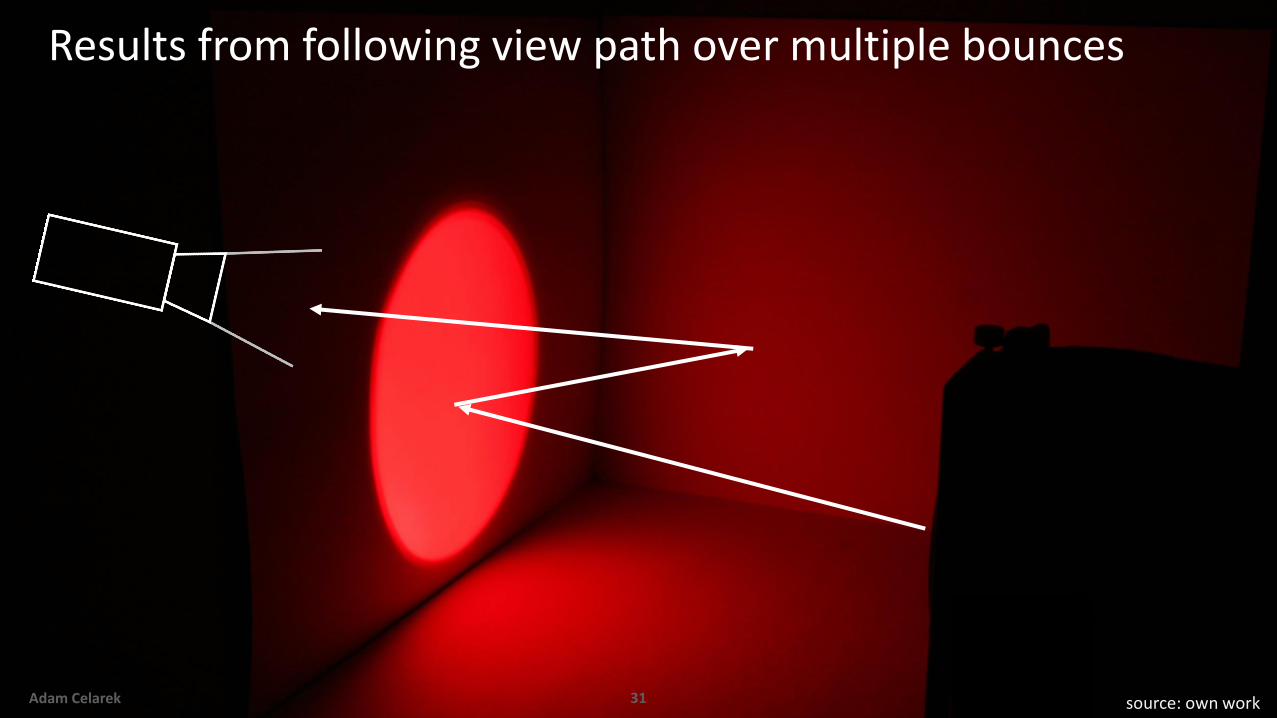
Results from following view path over multiple bounces
Adam Celarek 31 source: own work

Indirect Illumination
Difficult in real-time graphics – comes naturally in path tracing!
Rendering – Path Tracing Basics 32

Let’s go one step further!
Indirect Lighting with the Rendering Equation
Rendering – Path Tracing Basics 33
𝑥
𝑣 𝜔
𝐸 𝑥 → 𝑣 …... 𝐸𝑥
𝑓 𝑥, 𝜔 → 𝑣 ... 𝑓𝑟
𝑥′
𝐿 𝑥 → 𝑣 = 𝐸𝑥 +නΩ
𝑓𝑟 𝐿 𝑥 ← 𝜔 cos 𝜃𝜔 𝑑𝜔

Let’s go one step further!
Indirect Lighting with the Rendering Equation
Rendering – Path Tracing Basics 34
𝐿 𝑥 → 𝑣 = 𝐸𝑥 +නΩ
𝑓𝑟 𝐿 𝑥 ← 𝜔 cos 𝜃𝜔 𝑑𝜔
𝑣 𝜔
Let’s expand this!
𝑥′′
𝜔′𝑥
𝑥′

Let’s look at this new equation in detail…
Indirect Lighting with the Rendering Equation
Rendering – Path Tracing Basics 35
𝐿 𝑥 → 𝑣 = 𝐸𝑥 +නΩ
𝑓𝑟 𝐸𝑥′ +නΩ′𝑓𝑟′ 𝐿 𝑥′ ← 𝜔′ cos 𝜃𝜔′ 𝑑𝜔′ cos 𝜃𝜔 𝑑𝜔
𝑣 𝜔
𝜔′
𝑥′′
𝑥′
𝑥

A pattern emerges!
Indirect Lighting with the Rendering Equation
Rendering – Path Tracing Basics 36
𝑣 𝜔
𝜔′
𝑥′′
𝑥′
𝑥
𝐿 𝑥 → 𝑣 = 𝐸𝑥 +නΩ
𝑓𝑟 𝐸𝑥′ +නΩ′𝑓𝑟′ 𝐿 𝑥′ ← 𝜔′ cos 𝜃𝜔′ 𝑑𝜔′ cos 𝜃𝜔 𝑑𝜔

A real solution could go on much longer (ideally indefinitely)
Indirect Lighting with the Rendering Equation
Rendering – Path Tracing Basics 37
𝑣 𝜔
𝜔′ 𝜔′′
…
𝑥′′
𝑥′
𝑥
𝐿 𝑥 → 𝑣 = 𝐸𝑥 +නΩ
𝑓𝑟 𝐸𝑥′ +නΩ′𝑓𝑟′ … cos 𝜃𝜔′ 𝑑𝜔′ cos 𝜃𝜔 𝑑𝜔

Indirect Lighting with the Rendering Equation
With Monte Carlo integration, we might replace all ∫with ∑
Rendering – Path Tracing Basics 38
𝑣
𝜔j′
…
𝑥′′
𝑥′
𝑥
𝜔𝑖 𝜔𝑘′′
𝐿 𝑥 → 𝑣 = 𝐸𝑥 +1
𝑁
𝑖=1
𝑁
𝑓𝑟 𝐸𝑥′ +1
𝑁
𝑗=1
𝑁
𝑓𝑟′ … cos 𝜃𝜔𝑗
′1
𝑝(𝜔𝑗′)
cos 𝜃𝜔𝑖
1
𝑝(𝜔𝑖)

Indirect Lighting with the Rendering Equation
With Monte Carlo integration, we might replace all ∫with ∑
Rendering – Path Tracing Basics 39
𝑣…𝑥′
𝑥
𝜔𝑖
𝜔j′ 𝜔𝑘
′′
𝑥′′
𝜔𝑖
𝜔𝑖
𝜔j′
𝜔j′
𝜔𝑘′′
𝜔𝑘′′
𝐿 𝑥 → 𝑣 = 𝐸𝑥 +1
𝑁
𝑖=1
𝑁
𝑓𝑟 𝐸𝑥′ +1
𝑁
𝑗=1
𝑁
𝑓𝑟′ … cos 𝜃𝜔𝑗
′1
𝑝(𝜔𝑗′)
cos 𝜃𝜔𝑖
1
𝑝(𝜔𝑖)

Let’s implement this with recursion!
Rendering – Path Tracing Basics 40
v_inv = camera.gen_ray(px, py)
pixel_color = Li(v_inv)
function Li(v_inv)
x = scene.trace(v_inv)
f = 0
for (i = 0; i < N; i++)
omega_i, prob_i = hemisphere_uniform_world(x)
ray = make_ray(x, omega_i)
f += x.alb/pi * Li(ray) * dot(x.normal, omega_i) / prob_i
return x.emit + f/N
𝐿 𝑥 → 𝑣 = 𝐸𝑥 +1
𝑁
𝑖=1
𝑁
𝑓𝑟 𝐿 𝑥 ← 𝜔𝑖 cos 𝜃𝜔𝑖
1
𝑝(𝜔𝑖)

Each hemisphere integral computed with N samples (seems fair!)
Question: what to pick for N?
Let‘s start with something low
Like 4, 8, 16, 32
Let‘s see what we get…
Renderer never stops. Weneed a stopping criterion!
Let‘s run it!
Rendering – Path Tracing Basics 41

Adding hard stopping criterion
Rendering – Path Tracing Basics 42
v_inv = camera.gen_ray(px, py)
pixel_color = Li(v_inv, 0)
function Li(v_inv, D)
if (D >= NUM_BOUNCES)
return 0
x = scene.trace(v_inv)
f = 0
for (i = 0; i < N; i++)
omega_i, prob_i = hemisphere_uniform_world(x)
ray = make_ray(x, omega_i)
f += x.alb/pi * Li(ray, D+1) * dot(x.normal, omega_i) / prob_i
return x.emit + f/N

Let‘s run this again!
NUM_BOUNCES = 3
Samples for each sum and runtime
Rendering – Path Tracing Basics 43
N Time
4 3s
8
16
32

Let‘s run this again!
NUM_BOUNCES = 3
Samples for each sum and runtime
Rendering – Path Tracing Basics 44
N Time
4 3s
8 22s
16
32

Let‘s run this again!
NUM_BOUNCES = 3
Samples for each sum and runtime
Rendering – Path Tracing Basics 45
N Time
4 3s
8 22s
16 3m 33s
32

Let‘s run this again!
NUM_BOUNCES = 3
Samples for each sum and runtime
Rendering – Path Tracing Basics 46
N Time
4 3s
8 22s
16 3m 33s
32 43m 20s

Wisdom of the Day
The more samples, the better
…and also slower

Today’s Roadmap
Rendering – Path Tracing Basics 48
What is indirect illumination?
How do multiple bounces work?
Can we add other effects too?
Direct Lighting
Path Tracing v1.0 Path Tracing v0.5
Rendering
Equation
Recap
BSDF Interface Sample
Distribution
Russian Roulette

It‘s time to reconsider our approach
It works, but it‘s slow and the quality is not great
Also, this was only 3 bounces
Advanced effects can require much more than that!
Were we too naive, is path tracing doomed?
Definitely no!
There‘s a vast range of tools we can use to raise performance
Rendering – Path Tracing Basics 49

We can write this one big integral slightly differently
Reconsidering Sample Distribution
Rendering – Path Tracing Basics 50
𝐿 𝑥 → 𝑣 = 𝐸𝑥
+නΩ
𝑓𝑟 𝐸𝑥′ cos 𝜃𝜔 𝑑𝜔
+නΩ
𝑓𝑟නΩ′𝑓𝑟′ 𝐸𝑥′′ cos 𝜃𝜔′ cos 𝜃𝜔 𝑑𝜔′𝑑𝜔
+නΩ
𝑓𝑟නΩ′𝑓𝑟′න
Ω′′𝑓𝑟′′ 𝐸𝑥′′′ 𝑐𝑜𝑠(𝜃𝜔′′)cos 𝜃𝜔′ cos 𝜃𝜔 𝑑𝜔′′𝑑𝜔′𝑑𝜔
+ …
𝐿 𝑥 → 𝑣 = 𝐸𝑥 +නΩ
𝑓𝑟 𝐸𝑥′ +නΩ′𝑓𝑟′ … cos 𝜃𝜔′ 𝑑𝜔′ cos 𝜃𝜔 𝑑𝜔

𝐿 𝑥 → 𝑣 = 𝐸𝑥
+නΩ
𝑓𝑟 𝐸𝑥′ cos 𝜃𝜔 𝑑𝜔
+නΩ
𝑓𝑟නΩ′𝑓𝑟′ 𝐸𝑥′′ cos 𝜃𝜔′ cos 𝜃𝜔 𝑑𝜔′𝑑𝜔
+නΩ
𝑓𝑟නΩ′𝑓𝑟′න
Ω′′𝑓𝑟′′ 𝐸𝑥′′′ 𝑐𝑜𝑠(𝜃𝜔′′)cos 𝜃𝜔′ cos 𝜃𝜔 𝑑𝜔′′𝑑𝜔′𝑑𝜔
+ …
We can write this one big integral slightly differently
Reconsidering Sample Distribution
Rendering – Path Tracing Basics 51
Can you guess what
each of these lines does
for our final image?
𝐿 𝑥 → 𝑣 = 𝐸𝑥 +නΩ
𝑓𝑟 𝐸𝑥′ +නΩ′𝑓𝑟′ … cos 𝜃𝜔′ 𝑑𝜔′ cos 𝜃𝜔 𝑑𝜔

Reconsidering Sample Distribution
Rendering – Path Tracing Basics 52
𝐿 𝑥 → 𝑣 = 𝐸𝑥
+නΩ
𝑓𝑟 𝐸𝑥′ cos 𝜃𝜔 𝑑𝜔
+නΩ
𝑓𝑟නΩ′𝑓𝑟′ 𝐸𝑥′′ cos 𝜃𝜔′ cos 𝜃𝜔 𝑑𝜔′𝑑𝜔
+නΩ
𝑓𝑟නΩ′𝑓𝑟′න
Ω′′𝑓𝑟′′ 𝐸𝑥′′′ 𝑐𝑜𝑠(𝜃𝜔′′)cos 𝜃𝜔′ cos 𝜃𝜔 𝑑𝜔′′𝑑𝜔′𝑑𝜔
+ …

Reconsidering Sample Distribution
Rendering – Path Tracing Basics 53
𝐿 𝑥 → 𝑣 = 𝐸𝑥
+නΩ
𝑓𝑟 𝐸𝑥′ cos 𝜃𝜔 𝑑𝜔
+නΩ
𝑓𝑟නΩ′𝑓𝑟′ 𝐸𝑥′′ cos 𝜃𝜔′ cos 𝜃𝜔 𝑑𝜔′𝑑𝜔
+නΩ
𝑓𝑟නΩ′𝑓𝑟′න
Ω′′𝑓𝑟′′ 𝐸𝑥′′′ 𝑐𝑜𝑠(𝜃𝜔′′)cos 𝜃𝜔′ cos 𝜃𝜔 𝑑𝜔′′𝑑𝜔′𝑑𝜔
+ …

Reconsidering Sample Distribution
Rendering – Path Tracing Basics 54
𝐿 𝑥 → 𝑣 = 𝐸𝑥
+නΩ
𝑓𝑟 𝐸𝑥′ cos 𝜃𝜔 𝑑𝜔
+නΩ
𝑓𝑟නΩ′𝑓𝑟′ 𝐸𝑥′′ cos 𝜃𝜔′ cos 𝜃𝜔 𝑑𝜔′𝑑𝜔
+නΩ
𝑓𝑟නΩ′𝑓𝑟′න
Ω′′𝑓𝑟′′ 𝐸𝑥′′′ 𝑐𝑜𝑠(𝜃𝜔′′)cos 𝜃𝜔′ cos 𝜃𝜔 𝑑𝜔′′𝑑𝜔′𝑑𝜔
+ …

Reconsidering Sample Distribution
Rendering – Path Tracing Basics 55
𝐿 𝑥 → 𝑣 = 𝐸𝑥
+නΩ
𝑓𝑟 𝐸𝑥′ cos 𝜃𝜔 𝑑𝜔
+නΩ
𝑓𝑟නΩ′𝑓𝑟′ 𝐸𝑥′′ cos 𝜃𝜔′ cos 𝜃𝜔 𝑑𝜔′𝑑𝜔
+නΩ
𝑓𝑟නΩ′𝑓𝑟′න
Ω′′𝑓𝑟′′ 𝐸𝑥′′′ 𝑐𝑜𝑠(𝜃𝜔′′)cos 𝜃𝜔′ cos 𝜃𝜔 𝑑𝜔′′𝑑𝜔′𝑑𝜔
+ …

We used more samples for the contributions from longer light paths
The return-on-investment is not that great!
Reconsidering Sample Distribution
Rendering – Path Tracing Basics 56
1 sample N samples N² samples N³ samples

We have seen a different way of writing these results last time
The path integral form used a single integral for each bounce!
Reconsidering Sample Distribution
Rendering – Path Tracing Basics 57
𝐿 𝑥 → 𝑣 = 𝐸𝑥
+නΩ
𝑓𝑟 𝐸𝑥′ cos 𝜃𝜔 𝑑𝜔
+නΩ
𝑓𝑟නΩ′𝑓𝑟′ 𝐸𝑥′′ cos 𝜃𝜔′ cos 𝜃𝜔 𝑑𝜔′𝑑𝜔
+නΩ
𝑓𝑟නΩ′𝑓𝑟′න
Ω′′𝑓𝑟′′ 𝐸𝑥′′′ 𝑐𝑜𝑠(𝜃𝜔′′)cos 𝜃𝜔′ cos 𝜃𝜔 𝑑𝜔′′𝑑𝜔′𝑑𝜔
+ …

We have seen a different way of writing these results last time
The path integral form used a single integral for each bounce!
Reconsidering Sample Distribution
Rendering – Path Tracing Basics 58
𝐿 𝑥 → 𝑣 = 𝐸𝑥
+නΩ1
𝑓𝑟 𝐸𝑥′ cos 𝜃𝜔 𝑑𝜇( ҧ𝑥)
+නΩ2
𝑓𝑟 𝑓𝑟′𝐸𝑥′′ cos 𝜃𝜔′ cos 𝜃𝜔 𝑑𝜇( ҧ𝑥)
+නΩ3
𝑓𝑟𝑓𝑟′𝑓𝑟
′′ 𝐸𝑥′′′ 𝑐𝑜𝑠(𝜃𝜔′′)cos 𝜃𝜔′ cos 𝜃𝜔 𝑑𝜇( ҧ𝑥)
+ … fj( ҧ𝑥)

Let’s replace each integral with Monte Carlo integration again
Reconsidering Sample Distribution
Rendering – Path Tracing Basics 59
𝐿 𝑥 → 𝑣 = 𝐸𝑥
+1
𝑁
𝑖=1
𝑁
𝑓𝑟 𝐸𝑥′ cos 𝜃𝜔1
𝑝(𝜔)
+1
𝑁
𝑖=1
𝑁
𝑓𝑟 𝑓𝑟′𝐸𝑥′′ cos 𝜃𝜔′ cos 𝜃𝜔
1
𝑝 𝜔 𝑝(𝜔′)
+1
𝑁
𝑖=1
𝑁
𝑓𝑟𝑓𝑟′𝑓𝑟
′′ 𝐸𝑥′′′ 𝑐𝑜𝑠(𝜃𝜔′′)cos 𝜃𝜔′ cos 𝜃𝜔1
𝑝 𝜔 𝑝 𝜔′ 𝑝(𝜔′′)
+ …
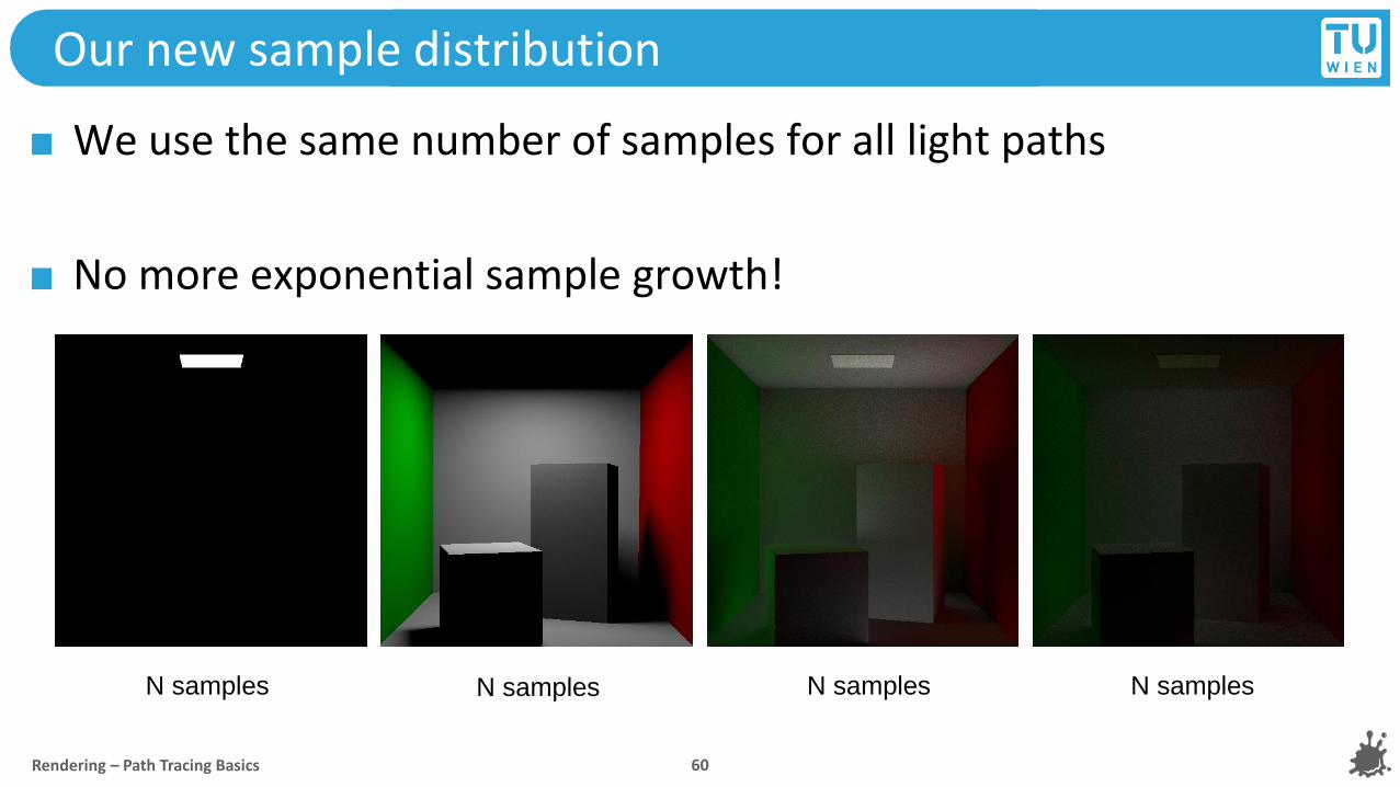
We use the same number of samples for all light paths
No more exponential sample growth!
Our new sample distribution
Rendering – Path Tracing Basics 60
N samples N samples N samples N samples

Let’s replace each integral with Monte Carlo integration again
Reconsidering Sample Distribution
Rendering – Path Tracing Basics 61
𝐿 𝑥 → 𝑣 = 𝐸𝑥
+1
𝑁
𝑖=1
𝑁
𝑓𝑟 𝐸𝑥′ cos 𝜃𝜔1
𝑝(𝜔)
+1
𝑁
𝑖=1
𝑁
𝑓𝑟 𝑓𝑟′𝐸𝑥′′ cos 𝜃𝜔′ cos 𝜃𝜔
1
𝑝 𝜔 𝑝(𝜔′)
+1
𝑁
𝑖=1
𝑁
𝑓𝑟𝑓𝑟′𝑓𝑟
′′ 𝐸𝑥′′′ 𝑐𝑜𝑠(𝜃𝜔′′)cos 𝜃𝜔′ cos 𝜃𝜔1
𝑝 𝜔 𝑝 𝜔′ 𝑝(𝜔′′)
+ …

We can again pull the sum to the front…
Reconsidering Sample Distribution
Rendering – Path Tracing Basics 62
𝐿 𝑥 → 𝑣 =1
𝑁
𝑖=1
𝑁
( 𝐸𝑥
+𝑓𝑟𝐸𝑥′ cos 𝜃𝜔1
𝑝(𝜔)
+𝑓𝑟𝑓𝑟′𝐸𝑥′′ cos 𝜃𝜔′ cos 𝜃𝜔
1
𝑝 𝜔 𝑝(𝜔′)
+𝑓𝑟𝑓𝑟′𝑓𝑟
′′𝐸𝑥′′′ 𝑐𝑜𝑠(𝜃𝜔′′)cos 𝜃𝜔′ cos 𝜃𝜔1
𝑝 𝜔 𝑝 𝜔′ 𝑝(𝜔′′)+ …)

…and rewrite to highlight the original recursion
We are back to a single sum for integration with recursion!
This also fits perfectly with our main loop and interface design
Reconsidering Sample Distribution
Rendering – Path Tracing Basics 63
𝐿 𝑥 → 𝑣 =1
𝑁
𝑖=1
𝑁
𝐸𝑥 + 𝑓𝑟 𝐸𝑥′ + 𝑓𝑟′ … cos 𝜃𝜔′
1
𝑝 𝜔′cos 𝜃𝜔
1
𝑝 𝜔

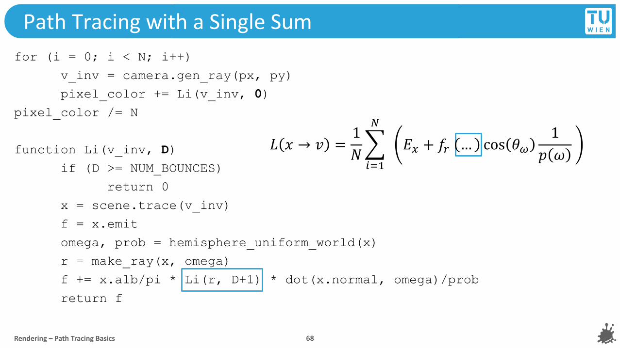
Path Tracing with a Single Sum
for (i = 0; i < N; i++)
v_inv = camera.gen_ray(px, py)
pixel_color += Li(v_inv, 0)
pixel_color /= N
function Li(v_inv, D)
if (D >= NUM_BOUNCES)
return 0
x = scene.trace(v_inv)
f = x.emit
omega, prob = hemisphere_uniform_world(x)
r = make_ray(x, omega)
f += x.alb/pi * Li(r, D+1) * dot(x.normal, omega)/prob
return f
Rendering – Path Tracing Basics 64
𝐿 𝑥 → 𝑣 =1
𝑁
𝑖=1
𝑁
𝐸𝑥 + 𝑓𝑟 … cos 𝜃𝜔1
𝑝 𝜔

Path Tracing with a Single Sum
for (i = 0; i < N; i++)
v_inv = camera.gen_ray(px, py)
pixel_color += Li(v_inv, 0)
pixel_color /= N
function Li(v_inv, D)
if (D >= NUM_BOUNCES)
return 0
x = scene.trace(v_inv)
f = x.emit
omega, prob = hemisphere_uniform_world(x)
r = make_ray(x, omega)
f += x.alb/pi * Li(r, D+1) * dot(x.normal, omega)/prob
return f
Rendering – Path Tracing Basics 65
𝐿 𝑥 → 𝑣 =1
𝑁
𝑖=1
𝑁
𝐸𝑥 + 𝑓𝑟 … cos 𝜃𝜔1
𝑝 𝜔

Path Tracing with a Single Sum
for (i = 0; i < N; i++)
v_inv = camera.gen_ray(px, py)
pixel_color += Li(v_inv, 0)
pixel_color /= N
function Li(v_inv, D)
if (D >= NUM_BOUNCES)
return 0
x = scene.trace(v_inv)
f = x.emit
omega, prob = hemisphere_uniform_world(x)
r = make_ray(x, omega)
f += x.alb/pi * Li(r, D+1) * dot(x.normal, omega)/prob
return f
Rendering – Path Tracing Basics 66
𝐿 𝑥 → 𝑣 =1
𝑁
𝑖=1
𝑁
𝐸𝑥 + 𝑓𝑟 … cos 𝜃𝜔1
𝑝 𝜔

Path Tracing with a Single Sum
for (i = 0; i < N; i++)
v_inv = camera.gen_ray(px, py)
pixel_color += Li(v_inv, 0)
pixel_color /= N
function Li(v_inv, D)
if (D >= NUM_BOUNCES)
return 0
x = scene.trace(v_inv)
f = x.emit
omega, prob = hemisphere_uniform_world(x)
r = make_ray(x, omega)
f += x.alb/pi * Li(r, D+1) * dot(x.normal, omega)/prob
return f
Rendering – Path Tracing Basics 67
𝐿 𝑥 → 𝑣 =1
𝑁
𝑖=1
𝑁
𝐸𝑥 + 𝑓𝑟 … cos 𝜃𝜔1
𝑝 𝜔
Path Tracing with a Single Sum
for (i = 0; i < N; i++)
v_inv = camera.gen_ray(px, py)
pixel_color += Li(v_inv, 0)
pixel_color /= N
function Li(v_inv, D)
if (D >= NUM_BOUNCES)
return 0
x = scene.trace(v_inv)
f = x.emit
omega, prob = hemisphere_uniform_world(x)
r = make_ray(x, omega)
f += x.alb/pi * Li(r, D+1) * dot(x.normal, omega)/prob
return f
Rendering – Path Tracing Basics 68
𝐿 𝑥 → 𝑣 =1
𝑁
𝑖=1
𝑁
𝐸𝑥 + 𝑓𝑟 … cos 𝜃𝜔1
𝑝 𝜔

Path Tracing with a Single Sum
for (i = 0; i < N; i++)
v_inv = camera.gen_ray(px, py)
pixel_color += Li(v_inv, 0)
pixel_color /= N
function Li(v_inv, D)
if (D >= NUM_BOUNCES)
return 0
x = scene.trace(v_inv)
f = x.emit
omega, prob = hemisphere_uniform_world(x)
r = make_ray(x, omega)
f += x.alb/pi * Li(r, D+1) * dot(x.normal, omega)/prob
return f
Rendering – Path Tracing Basics 69
𝐿 𝑥 → 𝑣 =1
𝑁
𝑖=1
𝑁
𝐸𝑥 + 𝑓𝑟 … cos 𝜃𝜔1
𝑝 𝜔

Path Tracing Implementations – Comparison
Rendering – Path Tracing Basics 70
3 bounces, 1 sum, N = 2048 3 bounces, 3 nested sums, N = 16

Wisdom of the Day
Your samples are precious
…put them where they matter!

How many bounces are enough?
Remember: if we want to be physically correct, then we must consider all possible light paths (i.e., journeys of photons)
Photons stop bouncing when they have been entirely absorbed
Problem: no real-world material absorbs 100% of incoming light
No matter how many bounces, the probability might never go to absolute zero → so we should never stop?
Rendering – Path Tracing Basics 72

Today’s Roadmap
Rendering – Path Tracing Basics 73
What is indirect illumination?
How do multiple bounces work?
Can we add other effects too?
Direct Lighting
Path Tracing v1.0 Path Tracing v0.5
Rendering
Equation
Recap
BSDF Interface Sample
Distribution
Russian Roulette

How do we handle infinity?
In many cases, most contribution comes from the first few bounces
Can we exploit this fact and make long paths possible, but unlikely?
Rendering – Path Tracing Basics 74
Number of bounces
N samples N samples N samples N samples N samples

How do we handle infinity?
In many cases, most contribution comes from the first few bounces
Can we exploit this fact and make long paths possible, but unlikely?
Rendering – Path Tracing Basics 75
Number of bounces
N samples N samples N samples <N samples? ≪N samples?

Russian Roulette (RR)
Pick 0 < 𝑝𝑅𝑅 < 1. Draw uniform random value 𝑥 in [0, 1) to decide
𝑥 < 𝑝𝑅𝑅: keep going for another bounce
𝑥 ≥ 𝑝𝑅𝑅: end path
The longer a path goes on, the more likely it is to get terminated
The probability of a ray surviving the 𝐷𝑡ℎ bounce is 𝑝𝑅𝑅𝐷
Whenever a path continues with another bounce, compensate for
its (un)-likeliness by weighting the returned color from 𝐿𝑖 with 1
𝑝𝑅𝑅Rendering – Path Tracing Basics 76

Both objects emit light
Very aggressive RR
Assume fixed 𝑝𝑅𝑅 =1
5
Most paths (4
5) fail to
capture the pink sphere
The Logic behind Russian Roulette
Rendering – Path Tracing Basics 77

Both objects emit light
Very aggressive RR
Assume fixed 𝑝𝑅𝑅 =1
5
Most paths (4
5) fail to
capture the pink sphere
The Logic behind Russian Roulette
Rendering – Path Tracing Basics 78

Both objects emit light
Very aggressive RR
Assume fixed 𝑝𝑅𝑅 =1
5
When we do hit it, thedivision by 𝑝 compensatesfor times where we missed it
The Logic behind Russian Roulette
Rendering – Path Tracing Basics 79
x5
x5
…
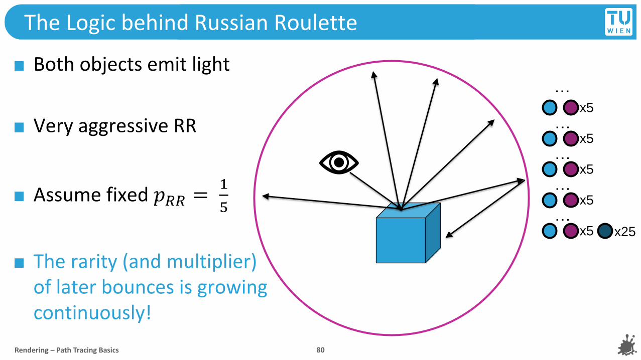
Both objects emit light
Very aggressive RR
Assume fixed 𝑝𝑅𝑅 =1
5
The rarity (and multiplier)of later bounces is growingcontinuously!
The Logic behind Russian Roulette
Rendering – Path Tracing Basics 80
x5
…x5
…x5
…x5
…x25

In code, you might be tempted to use1
𝑝𝑅𝑅𝐷 to compensate for RR
Don‘t! 1
𝑝𝑅𝑅is enough for each individual bounce!
If you use the recursive implementation, your effective RR compensation will grow with each bounce, all by itself…
Maybe look at pseudocode and ponder the previous slide for a bit
Russian Roulette Recursion Trap
Rendering – Path Tracing Basics 81
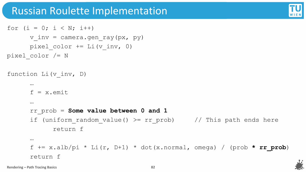
Russian Roulette Implementation
for (i = 0; i < N; i++)
v_inv = camera.gen_ray(px, py)
pixel_color += Li(v_inv, 0)
pixel_color /= N
function Li(v_inv, D)
…
f = x.emit
…
rr_prob = Some value between 0 and 1
if (uniform_random_value() >= rr_prob) // This path ends here
return f
…
f += x.alb/pi * Li(r, D+1) * dot(x.normal, omega) / (prob * rr_prob)
return f
Rendering – Path Tracing Basics 82

Russian Roulette..?
“…but if the possibility for infinitely long paths remains, doesn’t that mean that my renderer may take forever to finish?”
Almost certainly no
In practice, if you choose an adequate 𝑝𝑅𝑅, you are more likely to get struck by lightning while reading this than that ever happening
“Ok, cool, so the lower I choose 𝑝𝑅𝑅, the better, right? Can we just take something really small?” Well, not exactly.
Rendering – Path Tracing Basics 83

High 𝑝𝑅𝑅 vs low 𝑝𝑅𝑅, same number of samples
Rendering – Path Tracing Basics 84
𝑝𝑅𝑅 = 0.7: 50 seconds 𝑝𝑅𝑅 = 0.1: 35 seconds

High 𝑝𝑅𝑅 vs low 𝑝𝑅𝑅, same number of samples
Rendering – Path Tracing Basics 85
𝑝𝑅𝑅 = 0.7: 50 seconds 𝑝𝑅𝑅 = 0.1: 35 seconds

High 𝑝𝑅𝑅 vs low 𝑝𝑅𝑅, different number of samples
Rendering – Path Tracing Basics 86
𝑝𝑅𝑅 = 0.7: 50 seconds 𝑝𝑅𝑅 = 0.1, 4x as many samples: 150 seconds

High 𝑝𝑅𝑅 vs low 𝑝𝑅𝑅, different number of samples
Rendering – Path Tracing Basics 87
𝑝𝑅𝑅 = 0.7: 50 seconds 𝑝𝑅𝑅 = 0.1, 4x as many samples: 150 seconds

If 𝑝(𝑥) is low, but 𝑓(𝑥) is not → high contribution of rare events!
These “fireflies” tend to stick around!
Choose 𝑝𝑅𝑅 dynamically: compute itat each bounce according to possible color contribution („throughput“)
Fireflies and Throughput
Rendering – Path Tracing Basics 88
𝑝𝑅𝑅 = maxRGB
ෑ
𝑑=1
𝐷−1𝑓𝑟 𝑥𝑑 , 𝜔𝑑 → 𝑣𝑑 cos 𝜃𝑑
𝑝 𝜔𝑑 𝑝𝑅𝑅𝑑
𝑝𝑅𝑅 = 0.01
𝑝𝑅𝑅 = 0.5
𝑝𝑅𝑅 = 1.0
𝑝𝑅𝑅 = 1.0
𝑝𝑅𝑅 = 1.0
𝑝𝑅𝑅 = 1.0
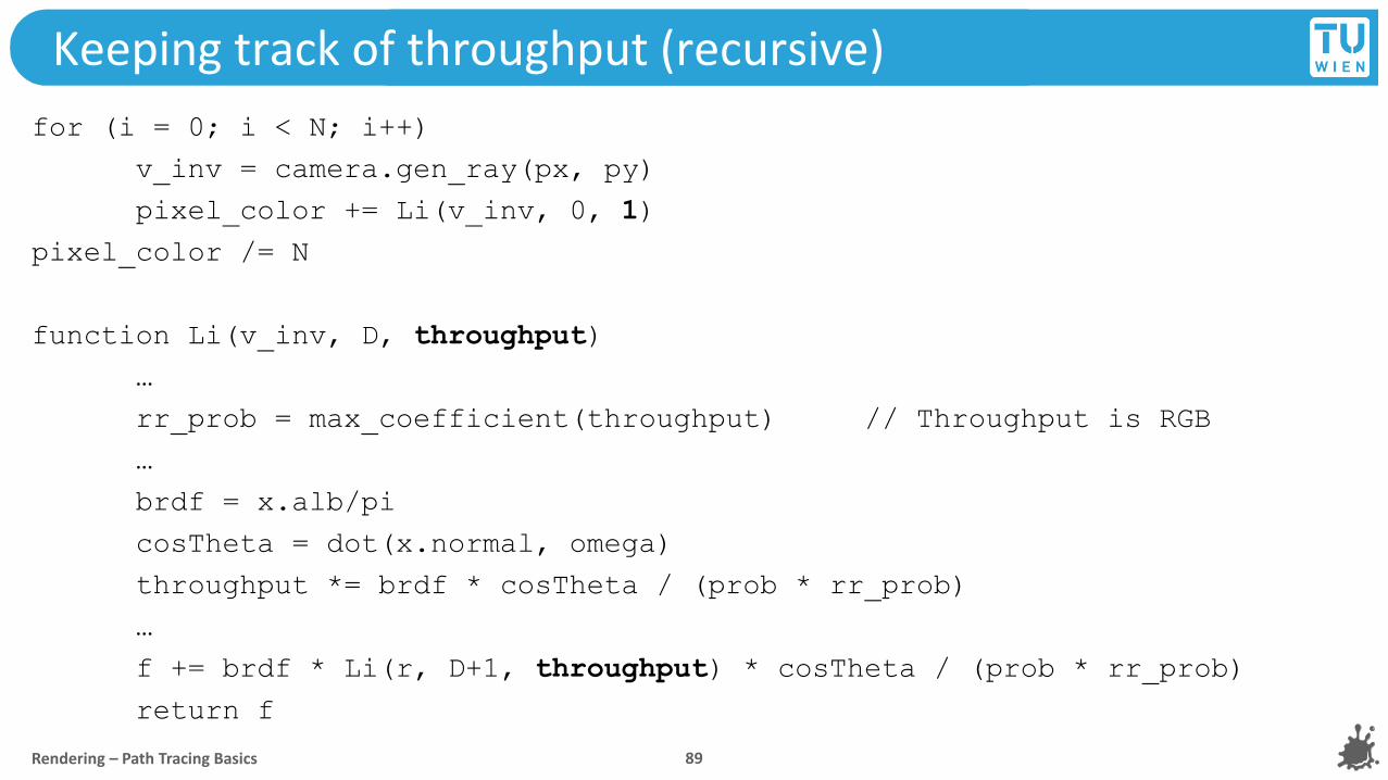
Keeping track of throughput (recursive)
for (i = 0; i < N; i++)
v_inv = camera.gen_ray(px, py)
pixel_color += Li(v_inv, 0, 1)
pixel_color /= N
function Li(v_inv, D, throughput)
…
rr_prob = max_coefficient(throughput) // Throughput is RGB
…
brdf = x.alb/pi
cosTheta = dot(x.normal, omega)
throughput *= brdf * cosTheta / (prob * rr_prob)
…
f += brdf * Li(r, D+1, throughput) * cosTheta / (prob * rr_prob)
return f
Rendering – Path Tracing Basics 89

Use guaranteed minimal path length before Russian Roulette starts
E.g., no Russian Roulette before the third bounce
Preserves a minimal path length for indirect illumination
Guaranteed bounces have 𝑝 = 1 always
Some materials absorb barely any incoming light (mirrors!)
Imagine two mirrors opposite of each other
Ray may bounce between them forever
Bad: limit bounces to a strict maximum
Better: clamp 𝑝𝑅𝑅 to a value < 1, e.g. 0.99
Russian Roulette Implementation Details
Rendering – Path Tracing Basics 90

Sample Distribution in Production Renderers
In practice, the distribution of samples is usually more dynamic:
Especially bounce 1 (direct light/shadows) receives more attention
Rendering – Path Tracing Basics 91
Number of bounces
medium high medium low lower

You can interpret the 𝑝𝑅𝑅 as an additional factor to MC integral
Originally, we divided by 𝑝 𝜔 to account for two things:
Scaling to approximate the whole domain (i.e., entire hemisphere)
Different probabilities of 𝜔 (not a factor with uniform sampling)2
3
Choosing and Compensating
Rendering – Path Tracing Basics 92

Choosing and Compensating
Probability density of following a particular 𝜔 changes to 𝑝 𝜔 𝑝𝑅𝑅Compensate for the fact that sometimes we chose to stop
Weight rare events higher (e.g., many bounces off dark materials)
We have to compensate whenever we pick one of multiple options
This is usually the case when you draw a random variable to decide on choosing one option and not the others
Rendering – Path Tracing Basics 93

Choosing and Compensating
Another example: picking a light source for light source sampling
For light source sampling, you can sample them all or just pick one
If you do pick only one, must compensate for making that choice!
Simplest: pick uniformly, multiply result by number of lights (why?)
Rendering – Path Tracing Basics 94

Wisdom of the Day
Monte Carlo is all about picking samples and then compensating
…and if you pick your samples carefully, we call it importance sampling

Today’s Roadmap
Rendering – Path Tracing Basics 96
What is indirect illumination?
How do multiple bounces work?
Can we add other effects too?
Direct Lighting
Path Tracing v1.0 Path Tracing v0.5
Rendering
Equation
Recap
BSDF Interface Sample
Distribution
Russian Roulette

Materials and the BSDF
We made a path tracer for diffuse materials, and diffuse only
Rendering – Path Tracing Basics 97
𝑛
𝑣
𝑥
Reflection Behavior Appearance

Capturing Path Behavior in a BSDF Data Structure
We made a solution that works, but only for diffuse materials
There are a lot of exciting other options
Specular
Glossy
…
Path tracer should allow adding materials without rewriting it all
Encapsulate material-dependent rendering factors in BSDF classRendering – Path Tracing Basics 98

Material-Dependent Factors
function Li(v_inv, D, throughput)
…
omega, prob = hemisphere_uniform_world(x)
…
brdf = x.alb/pi
throughput *= brdf * cosTheta / (prob * rr_prob)
…
f += brdf * Li(r, D+1, throughput) * cosTheta / (prob * rr_prob)
…
Rendering – Path Tracing Basics 99

function Li(v_inv, D, throughput)
…
omega, prob = hemisphere_uniform_world(x)
…
brdf = x.alb/pi
throughput *= brdf * cosTheta / (prob * rr_prob)
…
f += brdf * Li(r, D+1, throughput) * cosTheta / (prob * rr_prob)
…
Material-Dependent Factors
Rendering – Path Tracing Basics 100
Some materials will reflect incoming light
entirely in one single direction (mirrors).
Sampling the hemisphere in this case is
pointless! Also: we might be able to do
something smarter than uniform sampling

function Li(v_inv, D, throughput)
…
omega, prob = hemisphere_uniform_world(x)
…
brdf = x.alb/pi
throughput *= brdf * cosTheta / (prob * rr_prob)
…
f += brdf * Li(r, D+1, throughput) * cosTheta / (prob * rr_prob)
…
Material-Dependent Factors
Rendering – Path Tracing Basics 101
Super simple term that never
changes. Obviously, this only
makes sense if the amount of
reflected light is the same in all
directions, independent of 𝑣 and
𝜔 . Only a fully diffuse BSDF
gets away with this.

function Li(v_inv, D, throughput)
…
omega, prob = hemisphere_uniform_world(x)
…
brdf = x.alb/pi
throughput *= brdf * cosTheta / (prob * rr_prob)
…
f += brdf * Li(r, D+1, throughput) * cosTheta / (prob * rr_prob)
…
Material-Dependent Factors
Rendering – Path Tracing Basics 102
For some materials, like glass, this
cosine term is not needed, cancels
out or has to be removed for
reasons of energy conservation.

function Li(v_inv, D, throughput)
…
omega, prob = hemisphere_uniform_world(x)
…
brdf = x.alb/pi
throughput *= brdf * cosTheta / (prob * rr_prob)
…
f += brdf * Li(r, D+1, throughput) * cosTheta / (prob * rr_prob)
…
Material-Dependent Factors
Rendering – Path Tracing Basics 103
Many issues! Example: we could
have perfect mirrors that only
reflect in a single direction. Hence
the probability of other directions
is 0. Danger of division by 0!

Implement Basic Diffuse BRDFs with BSDF Interface
Nori BSDF class has three methods: eval, pdf, sample
Use auxiliary struct parameter bRec to pass 𝑣 (.wi ) and 𝜔 (.wo)
eval(bRec): evaluate material‘s ability to reflect light from 𝜔 to 𝑣
pdf(bRec) : compute the relative probability of sampling direction 𝜔
sample(bRec): make & store 𝜔 in bRec, compute material multiplier
Rendering – Path Tracing Basics 104
𝑛𝑣
𝜔

Implement Basic Diffuse BRDFs with BSDF Interface
Nori BSDF class has three methods: eval, pdf, sample
Use auxiliary struct parameter bRec to pass 𝑣 (.wi ) and 𝜔 (.wo)
eval(bRec): return 𝜌
𝜋if 𝑣, 𝜔 lie in hemisphere around 𝑛 (diffuse)
pdf(bRec) : return 1
2𝜋if 𝜔 lies in hemisphere around 𝑛 (all 𝜔 equal)
sample(bRec): create uniform 𝜔, return(cos 𝜃 ⋅ eval())/pdf()
Rendering – Path Tracing Basics 105
𝑛𝑣
𝜔

Using the New BSDF Class in Path Tracing Code
Isolates material-specific factor computations in a single function
Simplifies code and will make extension with other materials easy
function Li(v_inv, D, throughput)
…
omega, brdf_multiplier = sample(x, v_inv)
…
throughput *= brdf_multiplier / rr_prob
…
f += brdf_multiplier * Li(r, D+1, throughput) / rr_prob
…
Rendering – Path Tracing Basics 106

Path-Tracing is Multidimensional
We already know some of them:
Constructing a new ray after each bounce (2𝐷)
Evaluating RR continuation probability (𝐷)
…
Other possible choices we have not yet considered:
Lens coordinates (for depth-of-field) (2)
Time (for motion blur) (1)
…
Rendering – Path Tracing Basics 107
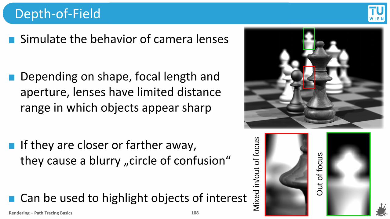
Depth-of-Field
Rendering – Path Tracing Basics 108
Simulate the behavior of camera lenses
Depending on shape, focal length and aperture, lenses have limited distancerange in which objects appear sharp
If they are closer or farther away,they cause a blurry „circle of confusion“
Can be used to highlight objects of interest
Mix
ed
in
/ou
t o
ffo
cu
s
Ou
t o
ffo
cu
s

Depth-of-Field in Path Tracing
Can simulate depth-of-field for a thin lens with focal length 𝑓[2]
Create camera ray 𝑟 through pixel as before
Find focal point 𝒇 along 𝑟 at distance 𝑓
Pick random location 𝑥, 𝑦 on the lens (2D disk) inside the aperture
Shoot camera ray from 𝑥, 𝑦 through 𝒇Rendering – Path Tracing Basics 109
𝑓
Close to focal length (sharp)
Far from focal length (blurred)
𝒇𝟏
𝒇𝟐
apert
ure

Motion Blur
Mostly an artistic effect to simulate a familiar camera phenomenon
Occurs when medium exposureis longer than rate of motion ofobjects in the captured scene
Can help convey the impression ofmoving objects in still image
In path tracing, all we need is an additional integrated time variableRendering – Path Tracing Basics 110

Motion Blur in Path Tracing
Option 1: make camera position a function of time 𝑡
Draw a random 𝑡, create adapted view ray 𝑟
Follow path through the scene
Check which triangles ray intersects
Option 2: make geometry a function of time 𝑡
Draw and store a random 𝑡, create view ray 𝑟
Follow path through the scene
Check which triangles ray intersects at 𝑡
Rendering – Path Tracing Basics 111
𝑝𝑜𝑠(0)
𝑝𝑜𝑠(𝑡)𝑝𝑜𝑠(0)
𝑝𝑜𝑠(𝑡)
Ray 𝑟 at time 𝑡
𝑝𝑜𝑠(0)
𝑝𝑜𝑠(𝑡)Ray 𝑟 at time 𝑡

Today’s Roadmap
Rendering – Path Tracing Basics 112
What is indirect illumination?
How do multiple bounces work?
Can we add other effects too?
Direct Lighting
Path Tracing v1.0 Path Tracing v0.5
Rendering
Equation
Recap
BSDF Interface Sample
Distribution
Russian Roulette

Everything that is wrong with our path tracer right now
So far, we only rendered very simple scenes (Cornell box)
What happens if we run a slightly more challenging scene?
Ajax bust, 500k triangles
Takes 17 hours (!) to geta boring, noisy image…
Is path tracing doomed (again)?
No! We will make better images in seconds!Rendering – Path Tracing Basics 113

Room for Improvement
Economize on samples – squeeze out whatever we can
Better sampling strategies (importance sampling)
Exploiting light source sampling (next-event estimation)
Combining sampling strategies (multiple importance sampling)
Improving our scene intersection tests
Build spatial acceleration structures
Optimized traversal strategies
Support spectacular specular, glossy and transparent materialsRendering – Path Tracing Basics 114

References and Further Reading
[1] Creating an Orientation Matrix or Local Coordinate System https://www.scratchapixel.com/lessons/mathematics-physics-for-computer-graphics/geometry/creating-an-orientation-matrix-or-local-coordinate-system
[2] Depth-of-Field Implementation in a Path Tracerhttps://medium.com/@elope139/depth-of-field-in-path-tracing-e61180417027
[3] Toshiya Hachisuka, Wojciech Jarosz, Richard Peter Weistroffer, Kevin Dale, Greg Humphreys, Matthias Zwicker, and Henrik Wann Jensen. 2008. Multidimensional adaptive sampling and reconstruction for ray tracing. ACM Trans. Graph. 27, 3 (August 2008)
[4] Ryan Overbeck, Craig Donner, and Ravi Ramamoorthi. Adaptive Wavelet Rendering. ACM Transactions on Graphics (SIGGRAPH ASIA 09), 28(5), December 2009.
Rendering – Path Tracing Basics 115