Remote Sensing of River Widths and Discharge Estimation for the Mainstem Congo River

Thesis

Presented in Partial Fulfillment of the Requirements for the

Bachelor of Sciences

At The Ohio State University

By

Nicholas Martin

The Ohio State University

2013

Approved by

Dr. Michael Durand

School of Earth Sciences

1

ABSTRACT

To conduct research in a study area such as the Congo basin is extremely difficult. The central African region is large and demanding to traverse. Obtaining the data necessary for calculating discharge in the field requires large amounts of time and funding; thus available data are very sparse. A much more efficient way to estimate discharge would be to estimate the variables from space-borne remote sensing measurements. The forthcoming NASA Surface Water and Ocean Topography satellite mission will measure river height, slope, and width. Not all variables necessary for determining discharge can be measured from remote sensing. The focus of this thesis is on measurement of river width via Landsat imagery and an automated width calculation algorithm. Depth was calculated using an approximation for reach-averaged depth from drainage area, adjusted for within-reach variations in river width. By

combining these two variables with a constant Manning’s and surface slope measurements, Manning’s open channel flow equation for discharge can be used. The measured mainstem Congo width ranged from 242 meters to 15,773 meters. The average estimated discharge of the mainstem was calculated to be 68,209 m3/sec, which was greater than what was recorded at the Kinshasa station by 25,136 m3/sec. It is hypothesized that the over estimation of discharge is due to the estimation of depth. Future improvements of RivWidth would improve automatic mainstem width measurement efficiency.

2

ACKNOWLEDGEMENTS

In accomplishing this thesis I have had support from multiple programs and people. First, I would like to thank two people that have supported me from the beginning, Douglas Alsdorf and Michael Durand. Together they had the grueling task of being my advisors. Helping me through all of my mistakes by never quitting on me they truly made my thesis possible for me. They both incorporated me into their two most important programs the Ohio State University’s Climate, Water and Carbon program and the NASA programs in Terrestrial Hydrology and in Physical Oceanography. I would also like to thank the School of Earth science and department of Geography for their support in providing the necessary resources in completing this thesis.

Others who assisted me in this thesis are C.K. Shum, Tamlin Pavelsky, Stephanie Konfal and Alex Rytel. All together they edited and guided me through intriguing conversations about many of these topics. They provided excellent questions regarding the processes that are need to determine river discharge. Thank you for forcing me to think critically about the topics presented in this paper.

Finally, I would like to thank four individuals that supported my decision to become a geologist all the way. When I truly reconsidered my life plans of becoming a geologist my family kept me on track. Thank you Michelle and John Martin, my parents, and Ron and Melissa Weber. Ron and Melissa have been to me an extra pair of parents. I could not have done this without the support of all mentioned and more. It is truly an honor to have all of you a part of my life.

3

CHAPTER 1

INTRODUCTION

1.1 The Objective of the Thesis

The goal of this thesis is to measure the river width of the Congo River, and, combined with measurements of river slope from prior work by Schaller (2010), to estimate its discharge. Width and slope measurements are derived from remote sensing data. Increasing the efficiency of the methods behind determining discharge variables can help determine river morphology on a larger scale. Understanding the movement of an environment (in this case the movement of a river) versus its surroundings is vital in every aspect of human life. It can determine a country’s border, economic gains, or even basic survival. By understanding specifics like water storage, biologists can learn why the Congo has such a large fish fauna population or by examining the widths and overall movement of a reach geologists can analyze river bank erosion.

The reason this region was selected is that it has limited data for this field of study. The challenges that are involved with gathering the variables for examining river dynamics in this area are what create this lack of information. The more direct methods of determining river dynamics must be approached in a different way. Going to a location such as the Congo and collecting data are impractical. The area is too large, politically-unstable and hard to traverse, making it practically impossible to study and understand fully. Using remotely-sensed data to gather variables such as river height and width can be beneficial in this area of study.

This region is economically and culturally important and as it grows more stable the prosperity in the region will grow. In the past few years a handful of African countries have developed faster than most countries in the world. Having the area researched extensively will only benefit those who live and work in this area. As regions grow the need for water grows especially fresh water. Therefore, understanding the areas hydrology will allow the surrounding countries to allocate their water resource much easier.

1.2 Project Background

This project was started at The Ohio State University to solidify a method of determining river dynamics. The Congo Basin was picked due to its lack of research and its vital importance to the African Continent. This continuation in the development of determining hydraulic information from spaceborne remote sensing will also assist in the evaluation of raw data produced from upcoming NASA mission Surface Water Ocean and Topography (SWOT) mission. This thesis builds upon work done by Ms. Lisa Schaller as part of a thesis at The Ohio State University School of Earth Sciences, 2010. Here, we use the same slope measurements used by Schaller, but measure river widths using remote sensing measurements, whereas Schaller had approximated widths from a global relationship. Moreover, we have obtained discharge measurements

4

from the Global Runoff Data Center (GRDC) to validate the discharge estimate from remote sensing.

1.3 Study Area 1.3.1 Location

The Congo River basin is the third largest river basin in the world (the first being the Amazon River in South America) and the largest in Africa (Lee et al., 2011). At roughly 3.7x106 km2 (Lee et al., 2011) the basin extends from latitude 09° 15ʹ N to 13° 28ʹ S and longitude 31° 10ʹ E to 11° 18ʹ E. The river starts in the East African Rift at the Great African Lakes: see Figure 1. The basin is surrounded by a series of mountains and equatorial ridges. Starting in the Northwest the Adamaua Mountains, the northern equatorial ridge in the North, the east African Highlands in the East, and the Crystal Mountains in the West and the southern equatorial ridge in the South form the boundary of the basin. From a political point of view the Congo River Basin encompasses 9 countries; Angola, Burundi, Cameroon, Central African Republic, Democratic Republic of the Congo, Republic of the Congo, Rwanda, Tanzania, and Zambia (Shahin, 2002).

Figure 1: The Congo River Basin is outlined in red and the Congo River is in the blue. Created in ArcGIS.

1.3.2 Climate and Hydrology

Similar to many locations on this planet, the climate of the Congo Basin’s climate is subjected to change brought on by sea surface temperatures (SST) and the El Niño-Southern Oscillation (ENSO). The SST in the Atlantic and Indian Oceans and the ENSO can cause changes in rainfall (Jury and Mpeta, 2009). The central area of the basin has no dry season; it is continuously supplied by rainfall. This is due to its equatorial

5

location. One-third of the basin is located in the northern hemisphere and two-thirds in the southern hemisphere (Shahin, 2002).

The Congo River extends ~4,700 km in length and has many major tributaries (Shahin, 2002). They include: the Sangha River, the Ubangi River, the Aruwimi River, the Tschuapa River and the Kasai River (Schaller, 2010). The origin of the river is Lake Tanganyika where it then flows into the Luapula River via Lake Banweulu. With the continuous precipitation in the basin the fluctuations of water storage is low (Shahin, 2002). The Congo Basin operates much differently than the more studied Amazon Basin. The Amazon drains relatively evenly because its network of floodplain channels is completely interconnected with the mainstem (Alsdorf & Melack, 2000). The Congo is not as well connected as the Amazon and when fluctuations in water storage occur the wetlands drain unevenly. For example, water levels in wetlands continue to stay high when water levels in the mainstem and even adjacent tributaries begin to drop (Lee et al., 2011).

1.3.3 Biology

From both an economic and scientific standpoint the importance of diversity in the Congo Basin is important. For example, the second most diverse fish fauna in the world survive in the basin. By understanding river dynamics, specific fish fauna in the basin can be studied to a greater extent. This plethora of fish species is directly tied to the high water seasons in September-October and May-June. During these times many fish species migrate into the wet prairies and swamps to breed. This large population of fish species allows the human populations in the region to survive because of the poor agricultural opportunities in the area. In terms of other animal life, the Congo has a variety of unique species that only live in its basin and rely either on the river networks like the hippopotamus or in the swamp lands such as the three species of crocodile and the gorillas in the north that live in the swamps year round (Campbell, 2005).

6

CHAPTER 2

DATA AND METHODS

2.1 Data

2.1.1 Shuttle Radar Topography Mission (SRTM)

The SRTM data were acquired by the use of two radar antennas aboard the space shuttle Endeavor for an 11-day mission. By using the interferometric synthetic aperture radar technique, elevations were determined by calculating the radar phase difference of both antennas which have a known distance apart of 60 meters. The purpose of the mission was to acquire high resolution topography images. Two resolutions were developed: 30 meter and 90 meter. The 30 meter resolution was only produced for the United States and 90 meter resolution produced everywhere else (Farr et al., 2007). The SRTM heights can be used to calculate river slope.

2.1.2 Hydrological data and maps based on SHuttle Elevation Derivaties at multiple Scales (HydroSHEDS)

HydroSHEDS is a large-scale mapping product that provides hydrographic information. It provides both raster and vector data. HydroSHEDS obtains its data from SRTM. The information it provides is essential to determining water boundaries and drainage direction (USGS HydroSHEDS, 2008). HydroSHEDS is essentially a basin delineation based on the SRTM heights. The HydroSHEDS streamlines were used as a consistent basis for unifying SRTM heights and slopes and Landsat widths in the processing described later in this thesis.

2.1.3 Land Satellite 5 & 7

The Landsat program was the first civil Earth-observing satellite program. It started in 1972 and continues with Landsat 8 which was launched February 11, 2013. Landsat 5 and 7 are optical images that have a resolution of 30x30 meters. Repeat coverage is on a 16-day interval (Landsat 7 Facts, 2013). Landsat data are used in this thesis for calculation of river width. All of the width data were calculated from either Landsat 5 or Landsat 7 during the month of February. Table 1 shows important characteristics of all Landsat data used. Fourteen images were used for the Congo River. The fourteen images are referenced throughout based on their path and row. The path and row is defined by the Worldwide Reference System (WRS-2). This system allows for a user to enter in two generic numerical values called a path and a row. This in turn produces the same tile scene for a multitude of the Landsat satellites (Landsat Science, 2013).

7

Table 1. Landsat data used. Landsat tile numbers refer to path / row.

Satellite Landsat Tile Tile Date Lower Left Lat/Lon

Landsat 7 180/60 Feb. 2000 -0.93493/17.79927

Landsat 7 181/61 Feb. 2003 -2.38546/15.9156

Landsat 7 174/64 Feb. 2003 -6.72128/25.79844

Landsat 7 178/59 Feb. 2003 0.50755/21.17615

Landsat 7 179/59 Feb. 2003 0.51012/19.62061

Landsat 7 180/59 Feb. 2003 0.5069/18.09034

Landsat 7 181/60 Feb. 2001 -0.93889/16.22496

Landsat 7 176/61 Feb. 2001 -2.38435/23.64069

Landsat 7 181/62 Feb. 2003 -3.83217/15.60614

Landsat 7 175/62 Feb. 2001 -3.82976/24.883

Landsat 7 175/63 Feb. 2001 -5.27422/24.57307

Landsat 5 174/63 Feb. 1999 -5.27836/26.13456

Landsat 5 176/60 Feb. 1995 -0.94595/24.00658

Landsat 5 177/59 Feb. 1987 0.5046/22.77197

Landsat 5 181/63 Feb. 1999 -5.28159/15.31226

2.1.4 Global Runoff Data Centre (GRDC)

The GRDC is an international data centre. Acting as a facilitator of hydrologic data for twenty years, the information from the GDRC was used as validation of the determination of discharge. The data used was the discharge at the Kinshasa station on February 2001 (Global Runoff Data Centre, 2013). The Kinshasa station being the only gauging station along the Congo River mainstem. This underscores the importance of developing a spaceborne program focusing on measuring river dynamics.

8

METHODS

The focus of this thesis is to measure the widths of the entire Congo River from satellite data, and to estimate river discharge. The variables needed for river discharge

are: width, depth, slope and an appropriate Manning’s for the entire study area. For

simplicity the Manning’s will be set to a constant value. Manning’s cannot be calculated from satellite imagery. Width is calculated using Pavelsky’s River Width algorithm (RivWidth). Slope is determined by using SRTM heights and finding the slope of the surface water. Whereas Manning’s equation for uniform flow requires use of

bathymetric slope (which we do not have), we here used the surface slope. Depth

calculations are estimated as well by using the formula (Moody & Troutman, 2002). The equation being used for determining discharge is Manning’s equation of open channel flow:

(

)

2.2.1 Water Mask Determination

Before running RivWidth an unsupervised classification had to be made. Then the combination of classes has to be made in order to segregate water from the rest of the classes. The default ENVI classification algorithms were used to perform the water mask determination. Finding Landsat images that are clear of cloud cover or mostly clear of cloud cover is one of the most time consuming parts of the analysis. Images for the downstream-most part of the Congo basin could not be identified due to persistent cloud cover. A native Landsat tile over the Congo mainstem is shown in Figure 2.

Figure 2: Original Landsat image of tile 178/59 (Path/Row).

9

After finding a usable image it is put through this classification process that ENVI offers and in doing this the user is required to pick the k-mean and iterations for the classification. This is dependent on the tile and can change. After classifying the image properly where water is identified in a separate class the combination of classes is then possible.

Figure 3: Unsupervised classification of tile 178/59 (Path/Row). The river is shown in yellow.

Figure 4: Water mask of tile 178/59 (Path/Row). The river is shown in yellow.

By combining all of the classes except for water the production of the water mask is complete. However, there are some stipulations with RivWidth. It cannot calculate the

10

widths of tributaries that are not directly connected to the main river. This means it will only take the widths of the largest river and the tributaries connected to it not tributaries that are on the tile and cut off from the edge of the tile.

2.2.2 River Width Identification

River widths were calculated by using an automated algorithm called RivWidth (Pavelsky & Smith, 2008). By taking existing binary water masks it calculates a centerline down the designated river. It then computes the width along each pixel on the centerline. This algorithm can process widths for any classified river image.

The delineation of the centerline is done through filters that smooth out high frequency noise and filters that detect rapid changes in intensity. These two filters allow for edge detection of the river. This then allows the algorithm to determine distances from each river pixel to the nearest non-river pixel. The filter delineates the centerline by identifying the pixels of less change (Pavelsky & Smith, 2008).

In the actual calculation of the river width the algorithm uses transects that are orthogonal to the centerline. This algorithm can also be used in multichannel rivers by segregating the islands and bars from the calculations and summing up the multiple segments of the river (Pavelsky & Smith, 2008).

When using RivWidth it is much more beneficial that the tributaries are not processed while processing the main river stem. After widths have been calculated the tributaries connected to the mainstem have to be removed manually so that the widths from the tributary are not calculated as part of the mainstem. This was done through Excel by simply finding the width points that deviate from the mainstem and removing them manually. After the removal of the tributary widths all of the remaining widths along the mainstem are conglomerated into one single Excel file and then run through a Matlab program that calculates the discharge along the flow distance of the river.

2.2.3 Manning’s

In considering the necessary parameters for this task there are two that cannot be

determined directly from satellite imagery. Manning’s is determined through recorded accounts of the study area river environment. In the case of the Congo River the

Manning’s is assumed to be 0.030. This value is for normal channels that are described as “clean, straight, full stage, no rifts or deep pools” or for mountain streams with “bottom: gravels, cobbles and few boulders” (Chow, 1959).

11

2.2.4 Slope

Slopes were determined from the water surface elevations, by measuring the change in elevation over length between pixels by using the HydroSHEDS flow distance data against the elevation data presented from the SRTM data. Considering the Congo’s topography the change in slope will be centimeters over kilometers (Schaller, 2010). In fact, the determination of slope presented is the same method developed by Schaller.

2.2.5 Depth

Reach average depth was calculated from average annual discharge. The relationship between the average annual discharge and the catchment area determined from the literature (Shahin, 2002),

The mean discharge estimates were applied to the depth formula:

This formula was developed through existing data sets in an attempt to calculate a universal scaling for width and depth (Moody and Troutman, 2002). This was used due to the fact that a method could not be devised to obtain depth measurement from remotely-sensed data.

Taking from the above calculation and using it as an average for depth in the below equation made it possible to calculate along every point in the flow path. This is simple an adjustment of depth based on width in sub-reach intervals.

(

)

Having estimates of width and depth, discharge estimates were calculated.

2.2.6 Discharge

Discharge was calculated at each height point. Widths were interpolated to the X- and Y- locations of each height pixel to calculate discharge. Depths were calculated at

every width point, leaving Manning’s the only constant in the equation. In order to analyze the discharge data produced, in-situ data from the GRDC Kinshasa station in the Democratic Republic of the Congo during the month of February was gathered.

12

CHAPTER 3

RESULTS AND FUTURE WORK

3.1 Results

3.1.1 Width (W)

Widths are shown in Figure 5. Downstream is on the left of Figure 5. The widths range from 242 meters to 15,773 meters and average 3,187 meters. Width generally increases in the downstream direction. However, there are noticeable points in which the Congo does not follow this simple rule, due to the change in the geographic environment, such as changing bedrock conditions and bed slope. For example, as the river flows from the highlands to the North where it changes to flat lowland forest environment/wetland it begins to widen. The width of the Congo is far greater than what would be expected given its discharge, compared with other rivers globally. As will be noted later, a river with the discharge measured at Kinshasha during February 2000 would be expected to be only 1,500 m in width. At its widest, the Congo is a factor of ten greater than this.

Figure 5: Widths as a function of flow distance.

The multiple gaps present in the raw widths are due to two things. First, gathering an image for a specific point in time while maintaining a cloud free image cannot always be obtained from Landsat. Therefore, not all the tiles are present for the mainstem of the Congo River. The end of the downstream region of the Congo mainstem was not calculated because the cloud coverage was too great. Secondly, the information at the extremities of each tile is inaccurate and had to be removed in order for the data to be

13

properly processed. At some points RivWidth included tributaries in the river widths, which had to be removed manually. However, Figure 5 does include some points along the river where RivWidth returned a smaller width along with a larger width for two co-located braids along the channel; the only known instances of this are at flow distances of 1.5x106 km, and 0.75x106 km. Aside from these, Figure 5 represents the spatial variability of the Congo mainstem river widths. Note that the standard deviation of the width data shown above is nearly 2,000 m, which is reflective of the significant spatial variations in the data.

Figure 6: Segment of Width estimates

In the above Figure 6 the width estimates oscillate. This is due to such things as bars or even different sediments that have different erosion rates. This characteristic of change is normal.

14

Figure 7: Image of signicant width change. Tile 181/62 (path/row).

From Figure 5, the dramatic narrowing of the river from approximately 10 km to 3 km in width at approximately 0.75x106 km flow distance is a remarkable feature of the Congo River, as the width generally increases in the downstream direction. Tile 181/62 (shown in Figure 7) shows the raw Landsat data where this river narrowing occurs. Note that this narrowing is close to where the river slope increases from 5.4 to 63 cm/km. Thus we hypothesize that the river width decreases in response to faster flow velocities while maintaining approximately the same discharge.

The extremities of the width data where the river segment reaches the edge of the tile will produce inaccurate data. RivWidth will measures the distance from the centerline to the edge of the tile not the edge of the riverbank. This produces inaccurate data and gaps when the data are collected into one file. There are points in which the oscillation of widths is greater than expected. These extremes are points where inside the tile the main stem is broken. Where the tile breaks it will cause widths to drop because it is calculating the centerline to the end of the break not the riverbank sides. These were removed from the dataset manually. This process is time-consuming and represents a place for future improvement of RivWidth.

15

Figure 8: Width comparison

A comparison of the estimated widths previously used (Schaller, 2010) to the measured widths produced in RivWidth is shown in Figure 8. The widths estimated are significantly different. The estimated widths are limited by the universal formula used to determine width from the average annual discharge (Moody and Troutman, 2002). The measured widths produced by RivWidth are limited only by the errors discussed in this thesis. The estimated widths are smaller than the measured widths.

3.1.2 Depth (Z)

Determining discharge estimates from catchment area and using the produced

estimation in the formula for the Congo seems practical. The method is simplistic and effective and is what was used to determine depth for this paper. The widths calculated from RivWidth were used to adjust the reach average depths on a sub-reach scale. This is where the manipulation of Moody and Troutman’s formula occurred. By putting the width data inside the depth formula the calculation of depth was possible on a sub-reach scale.

16

Figure 9: Depth estimates for both upstream and downstream of the Congo River.

As presented above in Figure 9 the variations in depth are due to the incorporation of the width information. The only foreseen issues are when the depth estimate is calculated with an inaccurate width measurement as discussed previously. As the width estimate decreases the depth estimate will increase. Another issue arises when the sub-reach calculation cannot compensate for the reach depth average. This issue is a product of using universal formulas to determine depth estimates. There are areas in every river which a generic formula will not produce accurate results.

3.1.3 Discharge

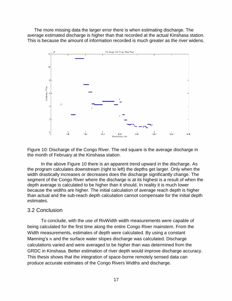
After determining width, slope, depth, and Manning’s variables discharge was calculated. By using Manning’s equation in Matlab for every point Q is calculated. Discharge generally increases with flow distance downstream (Figure 10). The discharge reaches at points considerable high rates. From the GRDC, the Kinshasa station has an average discharge of 43,073.778 m3/sec for the month of February in 2001. The average predicted discharge is 68,209 m3/sec. However, considering the missing data, the use of universal formulas for calculating variables, missing variables and image resolution of the Landsat and SRTM images a difference of 25,136 m3/sec was estimated. This estimation is simply an example that discharge is possible to be determined. A better form of validation would be to evaluate the estimated discharge to the discharge at the Kinshasa station.

17

The more missing data the larger error there is when estimating discharge. The average estimated discharge is higher than that recorded at the actual Kinshasa station. This is because the amount of information recorded is much greater as the river widens.

Figure 10: Discharge of the Congo River. The red square is the average discharge in the month of February at the Kinshasa station.

In the above Figure 10 there is an apparent trend upward in the discharge. As the program calculates downstream (right to left) the depths get larger. Only when the width drastically increases or decreases does the discharge significantly change. The segment of the Congo River where the discharge is at its highest is a result of when the depth average is calculated to be higher than it should. In reality it is much lower because the widths are higher. The initial calculation of average reach depth is higher than actual and the sub-reach depth calculation cannot compensate for the initial depth estimates.

3.2 Conclusion

To conclude, with the use of RivWidth width measurements were capable of

being calculated for the first time along the entire Congo River mainstem. From the

Width measurements, estimates of depth were calculated. By using a constant

Manning’s and the surface water slopes discharge was calculated. Discharge

calculations varied and were averaged to be higher than was determined from the

GRDC in Kinshasa. Better estimation of river depth would improve discharge accuracy.

This thesis shows that the integration of space-borne remotely sensed data can

produce accurate estimates of the Congo Rivers Widths and discharge.

18

3.3 Future Work

Areas in the RivWidth algorithm that need work are: The production of developing binary water masks in IDL that are compatible for multiple formats and the ability to calculate multiple river segments that are not connected to one another. Pavelsky’s method of calculating river widths is accurate and using it proved to be effective in calculating widths in such a large and remote area. Incorporating a water mask subprogram into the algorithm would be significantly more efficient. It removes the work required by the user and also forces the user to use a single software. An accuracy limitation with this method is in the ability of the image not RivWidth. Being limited to a 30x30-meter resolution leaves a notable amount of error in the calculation of width. This leaves only the largest rivers and tributaries to be calculated in the basin. Temporally this method has difficultly. Most satellites capable of being used for this process revolve around the planet and are not static which means that there is a period of time before it takes another image of that same area. In this case it is 16 days and if the image taken is covered by clouds it has to wait to take another image. In order to more accurately determine river width the only images used were images from February.

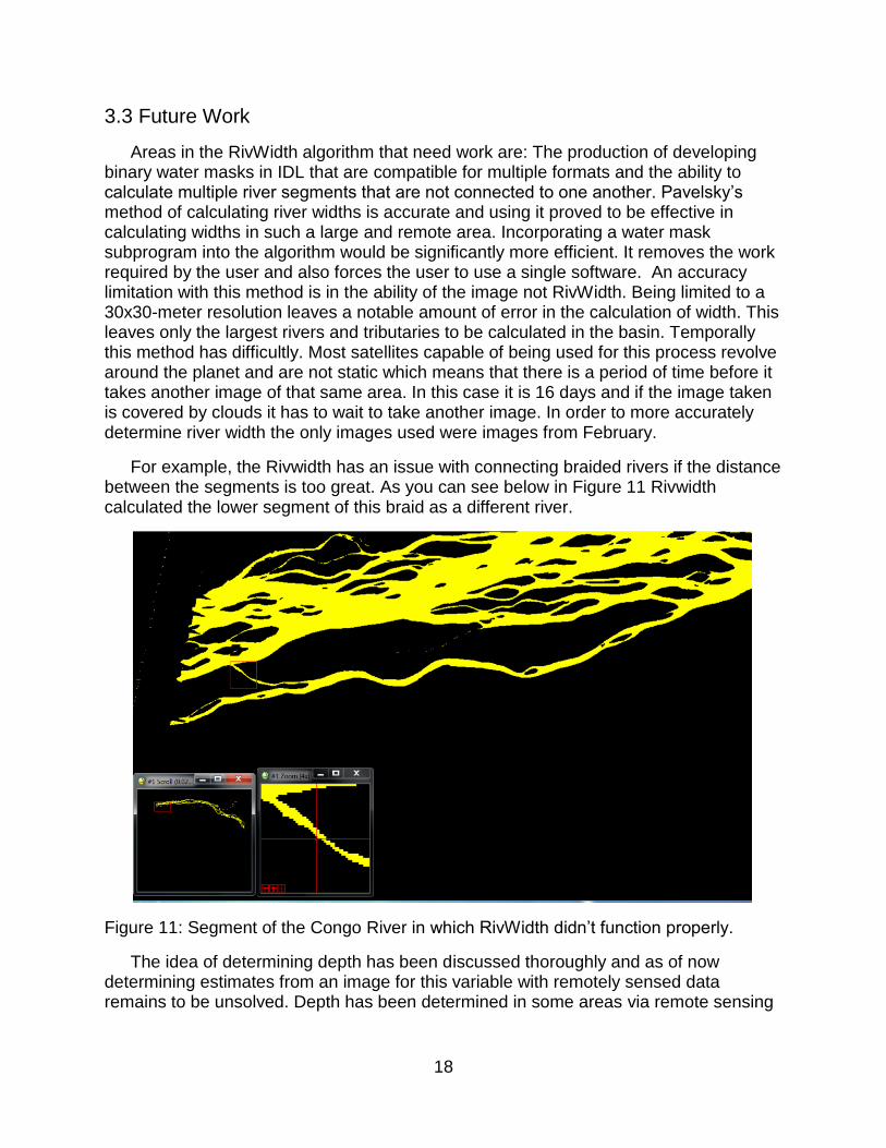
For example, the Rivwidth has an issue with connecting braided rivers if the distance between the segments is too great. As you can see below in Figure 11 Rivwidth calculated the lower segment of this braid as a different river.

Figure 11: Segment of the Congo River in which RivWidth didn’t function properly.

The idea of determining depth has been discussed thoroughly and as of now determining estimates from an image for this variable with remotely sensed data remains to be unsolved. Depth has been determined in some areas via remote sensing

19

from changes in a pixels digital number. However, those areas are shallow and clear and produced from aerial images not space-borne images.

20

REFERENCES CITED

Alsdorf, D. E., & Melack, J. M., 2000, Interferometric Radar Measurements of Water Level Changes on the Amazon Flood Plain: Nature, v. 404, I. 6774, p. 174

Campbell, D., 2005, The Congo River Basin, in Fraser, L.H., and Keddy, P.A., The world's largest wetlands: Ecology and conservation: Cambridge: Cambridge University Press., p. 149-165

Chow, V.T. 1959. Open Hydraulics: McGraw Hill Book Company, New York, N.Y., 680 pp.

Farr, T. G., Rosen, P. A., Caro, E., Crippen, R., Duren, R., Hensley, S., Kobrick, M., Alsdorf, D., 2007, The Shuttle Radar Topography Mission: Reviews of Geophysics, v. 45, n. 2 RG2004, doi:10.1029/2005RG000183

Global Runoff Data Centre, 2013, The GRDC,

http://www.bafg.de/GRDC/EN/01_GRDC/grdc_node.html;jsessionid=78D9ABDC0DAA19BB35233C66F88E30EB.live2052, accessed 2013.

Jury, M. R., & Mpeta, E. J., 2009, African climate variability in the satellite era:

Theoretical and Applied Climatology, v. 98, p. 279-291.

Landsat 7 Facts, http://geo.arc.nasa.gov/sge/landsat/l7.html, Accessed May, 2013 Landsat Science, 2013, http://landsat.gsfc.nasa.gov/about/wrs.html, Accessed July,

2013 Lee, H., Beighley, R. E., Alsdorf, D., Jung, H. C., Shum, C. K., Duan, J., Guo, J., and

Andreadis, K., 2011, Characterization of terrestrial water dynamics in the Congo Basin using GRACE and satellite radar altimetry: Remote Sensing of Environment, v. 115, p. 3530-3538.

Moody, J. A., & Troutman, B. M., 2002, Characterization of the spatial variability of

channel morphology: Earth Surface Processes and Landforms, v. 27, p. 1251-1266

Pavelsky, T.M., & L.C. Smith, 2008, RivWidth: A Software Tool for the Calculation of

River Widths from Remotely Sensed Imagery. IEEE Xplore. http://ieeexplore.ieee.org/xpl/freeabs_all.jsp?arnumber=4382932, Accessed May 2013

Schaller, L., 2010, Discharge of the Congo River Estimated from Satellite

Measurements [Undergraduate Thesis]: The Ohio State University, Columbus. Shahin, M, 2002, Hydrology and water resources of Africa: Dordrecht, Kluwer

Acedemic, 659 pp.

21

USGS HydroSHEDS, 2008, USGS HydroSHEDS: http://hydrosheds.cr.usgs.gov/hydro.php, Accessed May, 2013