Remote Sensing of Environment 152 (2014) 426–440

Contents lists available at ScienceDirect

Remote Sensing of Environment

j ourna l homepage: www.e lsev ie r .com/ locate / rse

Seasonal inundation monitoring and vegetation pattern mapping of theErguna floodplain by means of a RADARSAT-2 fully polarimetrictime series

Lingli Zhao 1, Jie Yang 1, Pingxiang Li 1, Liangpei Zhang ⁎State Key Laboratory of Information Engineering in Surveying, Mapping, and Remote Sensing, Wuhan University, Wuhan, 430079, China

⁎ Corresponding author at: No.129, Luoyu Road, WuhTel.: +86 13995556225.

E-mail address: zlp62@whu.edu.cn (L. Zhang).1 Tel.: +86 13995556225.

http://dx.doi.org/10.1016/j.rse.2014.06.0260034-4257/© 2014 Elsevier Inc. All rights reserved.

a b s t r a c t

a r t i c l e i n f o

Article history:Received 3 April 2014Received in revised form 26 June 2014Accepted 28 June 2014Available online 3 August 2014

Keywords:FloodplainPolarimetrySARRADARSAT-2Random forestsTrajectory analysis

The Erguna floodplain, located on the boundary of China, Russia, andMongolia, is a globally important breeding andstop-over site formanymigratory bird species. However, it has a fragile ecosystem and is facing severe impacts fromclimate change and human activities. Motivated by the high demand for spatial and temporal information aboutflooding dynamics and vegetation patterns, six fully polarimetric RADARSAT-2 images acquiredwith the same con-figurationwere explored to reveal the characteristics of thefloodplain. The evaluation of a set of polarimetric observ-ables derived from the series of polarimetric synthetic aperture radar (PolSAR) data was used to investigate thecharacteristics of the typical land-cover types in the floodplain. The behaviors of the polarimetric features highlightthe benefits of interpreting the scattering mechanism evolutions at different phenological and inundation stages.The vegetation and inundation patterns weremapped by a random forest (RF) classifier with the input of these po-larimetric observations. The results show that amulti-temporal classification can better capture the spatial distribu-tion of the vegetation pattern than single-temporal classifications, which often show a large variability due to theeffect of phenology and flooding. A hydroperiod map, which was generated by the time-series classification resultsof openwater, illustrates theflooding temporal dynamics and thehydrological regime. The twomain environmentalfactors that induced the changes in the backscattering – phenology and flooding –were identified based on the ag-gregated classification results of different phenological intervals. The spatial and temporal characteristics of thephenology- and flooding-induced changes were documented by the changes in the trajectories of three patchmetrics at the class level. The polarimetric features' importance scores derived from the RF classifier indicate thatthe intensity-related features are important for land-cover mapping. The HV intensity, in particular, achieves thehighest importance score. In addition, the volume scattering component shows a better performance among thecomposite features, revealing the importance of the quad-polarimetric information for floodplain interpretationand monitoring.

© 2014 Elsevier Inc. All rights reserved.

1. Introduction

Floodplains, adjacent to rivers, lakes, or oceans, are periodicallyflooded lands with dynamic hydrological processes (Bedient, Huber,Vieux, & Mallidu, 1988). They provide habitats for diverse wildlife andserve as buffers for extreme floods and droughts (Bayley, 1995; Junk,Bayley, & Sparks, 1989). A better understanding of the spatial distribu-tion and temporal changes of the vegetation and inundation patternsis a first important step for floodplain ecosystem protection, floodhazard mitigation, biodiversity sustainability, and land-use planning pur-poses (Bayley, 1995; Kerr et al., 2013; Marti-Cardona, Dolz-Ripolles, &

an City, Hubei Province, China.

Lopez-Martinez, 2013). This is especially crucial for the transboundaryriverfloodplainswhichoften stretch over several countries,where thehy-drological regimes are less understood. The future negative impacts of theregional, national, and international development plans on thesetransboundary floodplains are often poorly understood, due to the lackof detailed knowledge. The Erguna floodplain is just such a case (RwB -Rivers without Boundaries Coalition, 2011).

The Erguna floodplain, whose adjoining rivers are shared by China,Russia, and Mongolia, has a fragile ecosystem and faces severe impactsfrom climate change, urban growth, tourism, pasture harvest, and crop-land. It is a globally important breeding and stop-over site for manymi-gratory bird species, and it supports significant populations of at least 20bird species on the IUCN Red List (RwB–Rivers without BoundariesCoalition, 2011; UNDP, 2013). Drastically different cultures and modesof economic development, and the water use in Russia, China, andMongolia, make it very difficult to cooperate on environmentally

427L. Zhao et al. / Remote Sensing of Environment 152 (2014) 426–440

sound management of this transboundary basin (Goroshko, 2007).Specific water infrastructure facilities without a full assessment couldtrigger a dangerous pattern of environmental degradation for the area.For example, the Hailaer–Hulun water transfer project launched in2009 caused severe downstream impacts as a result of disturbing thenatural water cycle, and resulted in changes to the resting places of mi-grating birds, and alteration of the sedimentation and channel forma-tion pattern of the floodplain (Goroshko, 2007). A United Nationsdevelopment program named “Strengthening the management effec-tiveness of the protected area network in the Daxing'anling landscape”(UNDP, 2013) was launched in 2013 to ensure environmental sustain-ability. The Erguna floodplain is a part of the protected area, and thereis a high demand for spatial and temporal information about both theflooding dynamics and the vegetation patterns.

However, access to in situ data in floodplains is often limited by theirhighly dynamic characteristics, the remote locations, complex terrain,and large areas. Extensive and time-consuming field surveys are insuffi-cient to document floodplains changes at a landscape scale. Remotesensing techniques, which can acquire the information in a periodicmanner, provide a cost-effectivemeans tomonitor the seasonal changesand hydrological patterns of floodplains at a large scale. Landsat andMODIS time-series images have been used to map the land cover andmonitor the temporal duration of inundation areas for large lakes andwetlands (Ordoyne & Friedl, 2008; Ward et al., 2014; Zhao, Stein, &Chen, 2011). Nevertheless, when affected by cloudy conditions, opticalimages often cannot capture the temporal patterns of floods, especiallyin the rainy season. Synthetic aperture radar (SAR) can not only acquireperiodic images regardless of weather and time, but also provide valu-able information on biophysical and geophysical parameters, such assoil moisture (Bourgeau-Chavez, Leblon, Charbonneau, & Buckley,2013; Kornelsen & Coulibaly, 2013), vegetation biomass (Moreau & LeToan, 2003; Zhao, Yang, Li, & Zhang, 2014), and the structure of the scat-teringmedium (Zhao et al., 2013). In light of these benefits, a number ofstudies have been performed using SAR datasets over large floodplainsor wetlands, including the Amazon River floodplain (Arnesen et al.,2013; Martinez & Le Toan, 2007; Wang, Hess, Filoso, & Melack, 1995),the Negro River basin (Frappart, Seyler, Martinez, León, & Cazenave,2005), and the Doñana wetland (Marti-Cardona, Lopez-Martinez,Dolz-Ripolles, & Bladè-Castellet, 2010). Results using SAR images ac-quired by the ERS, ASAR, Cosmo-Skymed, and PALSAR sensors havealso been reported (Evans, Costa, Telmer, & Silva, 2010; Henderson &Lewis, 2008; Hong, Wdowinski, Kim, & Won, 2010; Ward et al., 2014).ASAR data were widely recognized as an important data source forwetland characterization, until the end of the ENVISAT mission inApril 2012 (ESA, 2013). Advanced techniques such as knowledge-based hierarchical classification (Arnesen et al., 2013; Evans et al.,2010), scattering indices (Hess, Melack, Novo, Barbosa, & Gastil,2003; Martinez & Le Toan, 2007), object-oriented segmentation(Arnesen et al., 2013; Pulvirenti, Chini, Pierdicca, Guerriero, &Ferrazzoli, 2011), and interferometric fringe patterns (Kim et al.,2009; Hong et al., 2010; Poncos, Teleaga, Bondar, & Oaie, 2013)have also been used to reveal the separability of the various land-cover types and to extract the flood-level information.

The interactions of radar signals with the complex land-cover typesfound inwetlands have been demonstrated from the followingmain as-pects: wavelength, incidence angle, temporal dynamics, environmentalfactors, and polarization. The penetration capability of radar signals in-creases the double bounce between stalks and thewater level, which fa-cilitates the monitoring of flooding under tree canopies. The longerwavelengths (L- or P-band) have been reported as being superior forflood detection in swamp forests (Hess, Melack, & Simonett, 1990),whereas the shorter wavelengths (C- or X-band) have been found tobe suitable for herbaceous marshes (Grings et al., 2006; Henderson &Lewis, 2008). The effect of the incidence angle is closely related to theother radar parameters and the vegetation type and structure (Costa &Telmer, 2006; Lang, Townsend, & Kasischke, 2008). Multi-incidence-

angle images have also been used to document the characteristics ofswamp forest by providing more complementary information (Langet al., 2008). Marti-Cardona et al. (2010) reported on the feasibility offlood mapping by incorporating various incidence angle images.In spite of these potential advantages,multi-temporal images are gener-ally regarded as being essential to capture the dynamic characteristics ofa study area (Henderson& Lewis, 2008). In addition, the highly dynamicnature of a floodplain is also affected by other changing environmentalfactors, such as vegetation development (Marti-Cardona et al., 2010)and the leaf-on/leaf-off condition (Lang et al., 2008; Townsend, 2001).With this in mind, the factors that induce the backscattering and scat-tering mechanism changes should be identified. This knowledge willbe beneficial for future floodplain planning and long-term hydrologicalmechanism analysis.

The interpretation of the backscattering changes of the land-covertypes in wetlands is limited when using single- or dual-polarization ob-servations. PolSAR,which acquires the target backscatteringwithmulti-ple channels in a coherent manner, allows a more in-depth explorationof the scattering mechanism. The copolarized phase difference (CPD) isregarded as a promising feature and has been used to enhance the iden-tification of flooded vegetation (Hess, Melack, Filoso, & Wang, 1995;Pope, Rejmankova, Paris, & Woodruff, 1997). Large absolute values ofCPD have been observed in flooded forest and fens by the use of polari-metric SIC-C data in the C- and L-band (Hess et al., 1995), and AIRSARdata in the L-band (Durden, Van Zyl, & Zebker, 1989). In recent years,target scattering decomposition methods have also been used to char-acterize wetlands. The double-scattering component derived frommodified four-component Yamaguchi decomposition has been used tocapture the seasonal changes of a reed area (Yajima, Yamaguchi, Sato,Yamada, & Boerner, 2008). Schmitt and Brisco (2013) detected floodedvegetation in a wetland in Canada through the use of a series ofRADARSAT-2 images by introducing the alpha angle fromCloude–Potti-er decomposition (Cloude & Pottier, 1997) to a curvelet-based changedetection algorithm. Roll-invariant target decomposition has also beenexplored to characterize wetland (Touzi, Deschamps, & Rother, 2007,2009). Touzi et al. found that the dominant scattering type magnitudeand phase make it possible to distinguish poor fens from shrubbogs, leading to a better understanding of marsh complex scatteringmechanisms, and they illustrated the potential and capability ofPolSAR data in wetland monitoring. Despite these promising fea-tures for wetland characterization, a more complete demonstrationof the interactions of radar signals with a highly dynamic floodplainduring the phenological stages and flood cycle needs to be docu-mented. Many different polarimetric features could be employedfor this purpose, and it is necessary to assess their different perfor-mances. The classification accuracies of different polarization combi-nations have been used to assess the performance of differentfeatures over wetlands (Betbeder et al., 2013; Turkar, Deo, Rao,Mohan, & Das, 2012). However, it is somewhat unfair to comparethese features independently, because the preferential informationcarried by each feature may be beneficial for different land-covertypes.

Motivated by the high demand for detailed information about flood-plain characterization, both spatial and temporal, we used a series offine-beam RADARSAT-2 images acquired during 2012 and 2013 overthe Erguna floodplain to: 1) demonstrate the superiority of C-bandPolSAR images in floodplain seasonal inundation monitoring and vegeta-tion pattern mapping; 2) illustrate the changes in the scattering mecha-nisms observed by C-band fully polarimetric SAR data for typical land-cover types at different flood states along the phenological profile;3) identify the factors that cause the variations in the land-cover classmapping and the changes in the spatio-temporal patterns (phenology-induced and flooding-induced changes are focused on in thispaper); and 4) investigate the importance of single-temporal andmulti-temporal polarimetric features for floodplain monitoring,based on the RF algorithm.

Fig. 2. Precipitation and maximum temperature per month for 1945–2000 (orange) andthe data of 2013 (cyan) for the study area.

428 L. Zhao et al. / Remote Sensing of Environment 152 (2014) 426–440

2. Study area and experimental data

2.1. Study area and background

The Erguna floodplain extends over the Erguna River and its threetributaries (the Genhe River, Deerbugan River, and Hawuer River) asshown in Fig. 1. The study area is located on the Genhe River, and is in-dicated by the red polygon in Fig. 1. The topography of the floodplain isrelatively flat, with an average water-surface gradient of 0.73‰. Theflood extension undergoes seasonal changes from May to October inthe floodplain. Precipitation and maximum temperature data collectedat the nearest rain gauge stations were obtained from the ChinaMeteo-rological Data Sharing Service System (http://cdc.cma.gov.cn/). Theaverage annual precipitation in the regionwas about 3738mmbetween1954 and 2000, with the largest amount of rainfall being observedbetween July and August, as shown in Fig. 2. In 2013, the 50-year returnperiod rainfall occurred, and the rainfall was significantly higher thanthe average annual precipitation.

The active and complex meandering process in the floodplain hasled to the formation of multiple oxbow lakes and complex mosaics ofreed beds, willow thickets, meadows, and sedge bog habitats. Duringthe low-water season, the landscape of the floodplain mainly consistsof forest (Fig. 3a), reeds and sedges in bog areas (Fig. 3b), and meadow(Fig. 3c). The forest consists of tall and dense trees such as Choseniaarbutifolia and Populus suaveolens, with a height of between 5 and25 m, which are commonly found along the meanders of the river. Inthe rainy season, there are areas of low-lying meadow (Fig. 3d) andpoint bars (Fig. 3e), and some plants in the bog areas become sub-merged. During autumn, the meadows are harvested and bundled byfarmers (Fig. 3f). The aquatic plants in the bog also die back and are sub-sequently spread over the ground surface as the flooding recedes(Fig. 3g). As a result of the increases in both land reclamation and tourism,farmland (Fig. 3h) and buildings (Fig. 3i) are occupyingmore andmore ofthe floodplain.

2.2. RADARSAT-2 images and preprocessing

Six C-band quad-polarimetric RADARSAT-2 images were acquiredwith the same configuration from September 2012 to August 2013.

Fig. 1. Location of the study area.

The parameters of the images are shown in Table 1 (Morena, James, &Beck, 2004). The nominal pixel spacing in the azimuth and range direc-tionwas 5.1 × 4.7m, and the swathwidthwas 25 × 25 km. The beam ofall the images was FQ18, with the incidence angle ranging from 37.4° to38.9° to avoid the effect of the incidence angle. The repeat cycle was24 days. The related rainfall of 24 days and 5 days before the acquisitiondate of each image is shown in Table 1.

Two free open-source software packages – the Next ESA SAR Tool-box (NEST, http://nest.array.ca/web/nest) and the PolSARpro SAR DataProcessing and Educational Tool (http://earth.eo.esa.int/polsarpro/) –were used in the preprocessing of the SAR datasets. A 7 × 7 Lee filter(Lee, Grunes, & de Grandi, 1999) was first used on all the images to sup-press the speckle noise. All the SAR images were then geometricallycorrected by the Range-Doppler model embedded in NEST, with the as-sistance of an SRTM 90 m digital elevation model (DEM) (http://srtm.csi.cgiar.org/). The geometrically rectified images were registered andresampled to a scale of 8 m, with root-mean-square errors (RMSE) ofless than one pixel in both the X- and Y-directions. The pseudo-colorcomposite image by |Shh − Svv|2 of 2013-07-10 (red), |Shh + Svv|2 of2013-05-23 (blue), and |Shv|2 of 2013-08-03 (green) was overlaid onthe SRTM DEM, as shown in Fig. 4. The flat valley area was extractedusing the registered SRTMDEM to eliminate the effect of themountains.

2.3. Ancillary data and preprocessing

2.3.1. LiDAR and aerial CCD imagesFrom August to September of 2012, 24 aerial survey flights were

conducted over part of the floodplain. A Leica RCD105 digital framecamera and a Leica ALS60 airborne laser scanner equipped with aLeicaWDM65waveformdigitizermodulewere used to acquire CCD im-ages and LiDAR (light detection and ranging) data of a 0.5 m resolution.The flight lines in the survey had an overlap of about 53%. Survey pointsmeasured by a differential global positioning system (DGPS) were usedto validate the accuracy. The LiDAR datasets were used to generate theDEM, digital surface model (DSM), and canopy height model (CHM)products, with a spatial resolution of 0.5 m. The products and the CCDimages were used to assist with the selection of the ROIs of the trainingand test samples for the vegetation pattern mapping.

2.3.2. Field dataGround measurements near-coincident to the acquisitions of the

SAR images were collected between September 2012 to August 27th2013, with the aim being to investigate the spatial configuration of thefloodplain and the vegetation development. Photos of each typicalland-cover type were also acquired, to provide ground reference data

Fig. 3. Illustrations of themain landscape types and their status, as observed in the Erguna floodplain: a) river meanderwith forest; b) bog; c) productivemeadow; d) low-lyingmeadow;e) point bar in dry season; f) harvestedmeadow in autumn; g) lodged aquatic plants in bog during flooding recession; h) farmland cultivation around the floodplain; i) buildings for tourism inthe floodplain.

429L. Zhao et al. / Remote Sensing of Environment 152 (2014) 426–440

for the training and accuracy assessment. In addition, the height andwet-weight of the grass were collected to identify the changes in thebiomass and vegetation structure.

3. Method

3.1. ROI definition

According to the ancillary data and field campaigns, five main land-cover types were identified for the floodplain: open water, meadow,point bar, bog, and forest. Their ground references are shown in Fig. 5.Different ROIs were selected for these classes, according to their status

Table 1Characteristics of the C-band quad-polarimetric RADARSAT-2 images and the related rainfall o

Acquisition date Mode Incidence angle(degree)

Local time

2012-09-01 FQ18 37.4–38.9 6:00 pm2013-05-23 FQ18 37.4–38.9 6:00 pm2013-06-16 FQ18 37.4–38.9 6:00 pm2013-07-10 FQ18 37.4–38.9 6:00 pm2013-08-03 FQ18 37.4–38.9 6:00 pm2013-08-27 FQ18 37.4–38.9 6:00 pm

at each phase. Farmland parcels were first extracted manually, becausethe different crop types exhibited inconsistent backscattering levelsalong the temporal profile. To reduce the bias, the training and test sam-ples were randomly selected from the selected ROIs.

3.2. Characteristics of the polarimetric features of the different classes

A set of polarimetric observations is presented to delineate the scat-teringmechanisms of the typical land-cover types in thefloodplain overeach phase. The observations and their physical descriptions are shownin Table 2. Backscattering (σHH

0 , σHV0 , σVV

0 ) and total span are the basic in-formation carried by the SAR data. The copolarized correlation

f 24 days and 5 days before the acquisition date of each image.

of acquisition Rainfall 24 days (mm) Rainfall 5 days (mm)

29.2 4.134.7 6.9

114.8 34.5106.8 56.4197.8 25.0127.5 4.9

Fig. 4. The RADARSAT-2 pseudo-color image as a color composite by |Shh − Svv|2 of 2013-07-10 (red), |Shh+ Svv|2 of 2013-05-23 (blue), and |Shv|2 of 2013-08-03 (green). The back-ground is the SRTM DEM.

Table 2Polarimetric observations used in the paper.

Polarimetricparameters

Physical description

σHH0 , σHV

0 , σVV0 Backscattering coefficient of the HH, HV, and VV

polarizations.span Total backscattering of the three polarizations.γ Copolarized ratio of the backscattering of VV and HH.ρco = |ρHHVV| Copolarized correlation coefficient between the HH and VV

polarizations.CPD Copolarized phase difference between the HH and VV

polarizations.H, α, A Entropy, alpha, and anisotropy derived from Cloude

decomposition.odd, dbl, vol, hlx Surface scattering, double scattering, volume scattering, and

helix scattering components from Yamaguchidecomposition.

430 L. Zhao et al. / Remote Sensing of Environment 152 (2014) 426–440

coefficient (|ρHHVV|) measures the spatial elements' scattering random-ness or the attenuation of the scattering medium (Lopez-Sanchez,Cloude, & Ballester-Berman, 2012; Nghiem, Kwok, Yueh, &Drinkwater, 1995). A high CPD value indicates the occurrence of doublescattering. Scatter mediums dominated by volume or surface scatteringexhibit a low CPD approaching zero (McNairn, Duguay, Brisco, & Pultz,2002). Three parameters – entropy (H), alpha (α), and anisotropy (A)– are derived from Cloude decomposition (Cloude & Pottier, 1997). H,ranging from 0 and 1, describes the scattering randomness. α indicatesthe dominant scattering mechanism, and lies between 0° and 90°. A,which is the complement of entropy, represents the relative power ofthe second and third scattering mechanisms. The four scattering com-ponents – surface scattering (odd), double scattering (dbl), volume scat-tering (vol), and helix scattering (hlx) from Yamaguchi decomposition(Yamaguchi, Moriyama, Ishido, & Yamada, 2005) – were normalizedto intuitively show the scattering mechanism of the land-cover typesin the floodplain.

Mean values and absolute changes in the multi-temporal polari-metric observations were derived to capture the pattern of change ofthe floodplain. The absolute change estimator (ACE) developed byQuegan, Le Toan, Yu, Ribbes, and Floury (2000) was selected to assessand quantify the temporal variations across the series of images. TheACE value is the logarithm of the ratio between any dates within themulti-temporal datasets, and it gives positive values in dB. The largerthe feature changes between two images, the greater the value of ACE.

Fig. 5. Selected ROIs for the main land-cover types in the study area.

It has been used in feature reduction and multi-temporal hierarchicalclassification by threshold segmentation (Martinez & Le Toan, 2007).We use the ACE features and the mean features for the multi-temporalclassification in the later sections.

3.3. Land-cover mapping and hydroperiod monitoring

The RF algorithm (Breiman, 2001) is an ensemble classifier thatbuilds large numbers of decision trees, based on bootstrapped samplesof the training data. “Bagging” and random selection of the featuresare combined to control the variation in the training. About two-thirdsof the training samples are randomly selected to construct each tree.The remaining samples are used to generate the out-of-bag error(OOB error). The output is determined by amajority vote of the classifi-er ensemble. The RF classifier can be trained on large, very high-dimensional datasets, without significant overfitting. It does not dependon the distribution of the data, and it tolerates a significant amount ofnoise, which is usually high for SAR data. A Fortran implementation ofthe RF algorithm is freely available at http://www.stat.berkeley.edu/breiman/RandomForests/. The RF algorithm can be used not only forclassification and prediction, but can also be used for variable im-portance assessment. Variable selection frequency (Loosvelt, Peters,Skriver, De Baets & Verhoest, 2012), Gini importance (Friedman,2001), and permutation importance (Breiman, 2001) have all beenused as variable importance measures. The last measure describes thedifferences in the prediction accuracy before and after permuting thevariable of interest, and is chosen in this paper. It takes into accountthe impact of each variable individually, as well as its interaction withthe other input variables. Importance measures have also been usedfor feature selection or uncertainty assessment in PolSAR classification(Loosvelt, Peters, Skriver, De Baets, et al., 2012; Loosvelt, Peters,Skriver, Lievens, et al., 2012). Here, we use the importance scores to as-sess the polarimetric features' contribution to the floodplain land-covermapping.

The area of open water in the classification results indicates the sea-sonal dynamics of the inundated area. To analyze the dynamics of theinundation, open water extracted from the single-temporal classifica-tion results was used to produce a flood hydroperiod map. The mapshows the area that is subjected to flooding, although we cannot ascer-tain the true inundation time for each area from the six images. Theprobability of inundation p(i,j) is defined as:

p i; jð Þ ¼

XN

k

dk

Nð1Þ

where N is the total number of phases, which is six for this study; and dkindicateswhether the area located at (i, j) isflooded,with a value of 0 or 1.

431L. Zhao et al. / Remote Sensing of Environment 152 (2014) 426–440

3.4. Trajectory analysis

Trajectory analysis is often used to discover the land-cover changetrend of an area (Mertens & Lambin, 2000; Zhou, Li, & Kurban, 2008a;Zhou, Li, & Kurban, 2008b). The interannual land-cover conversion canbe interpreted according to the changing profile and the context of thestudy. In general, trajectories are constructed at the pixel level for theindividual land-cover classes, using the classification results of all thephases (Petit, Scudder, & Lambin, 2001; Zhou et al., 2008a). However,there can be a wide variety of possible land-cover change trajectories.A trajectory profile is also often affected by different factors, and canbe difficult to interpret. To reduce the complexity of the trajectory pro-fileswhen using all the classes, the land-covermapping results betweentwo conjoint time points were aggregated into three generic classes,namely the non-changed class, the phenology-induced class, and theflooding-induced class. Thanks to this aggregation method, we can re-duce the dependence of the trajectories on the single-temporal classifi-cation accuracy.

The trajectories of the class metrics were established based on “bi-temporal” maps, to show the spatio-temporal patterns of the changesinduced by the different environmental factors. The class metricswere calculated in the FRAGSTATS 4.2 software package (http://www.umass.edu/landeco/research/fragstats, McGarigal, Cushman, & Ene,2012), which is designed to compute a wide variety of landscape met-rics for categorical map patterns. In this study, three metrics – the per-centage of landscape (PLAND), the normalized landscape shape index(NLSI), and the interspersion and juxtaposition index (IJI) –were select-ed. PLANDquantifies the abundance of each class in the area, and rangesbetween 0 and 100%. It approaches 0 when the corresponding class israre in the area, and equals 100% when there is a single class in thearea. NLSI, which ranges from 0 to 1, measures the aggregation of aclass. It is equal to 0 when there is a single square class in the area,and it increases with the disaggregation of the class. IJI denotes the in-terspersion and juxtaposition for all the presented classes, and rangesfrom 0 to 100%. It approaches 0 when the corresponding class is adja-cent to only one other class, and is equal to 100%when the correspond-ing class is equally adjacent to all the other classes. The class metricswere used to identify the spatial and temporal patterns of the affectedarea by different factors.

4. Results and discussion

Statistics of the parameters are presented to allow an investigationof the scattering behaviors of the land-cover classes in various floodinglevels and stages. The capability of single- and multi-temporal C-bandpolarimetric data for land-cover mapping is illustrated. The land-covertypes' separation at different phases and their distribution patterns aredemonstrated by the classification results generated by the RF classifier.A hydroperiod map is also given to allow a deeper exploration of thehydrological regime. The trajectories of the three class metrics areexplored to show the spatial and temporal characteristics of theflooding-induced and phenology-induced changes. The contribution ofthe polarimetric features to single-temporal and multi-temporal land-cover mapping of the Erguna floodplain is also presented and discussed.

4.1. Backscattering analysis

In the following subsections, analysis of the four intensity-relatedobservations of σHH

0 , σVV0 , σHV

0 , and span, and the eight well-known po-larimetric descriptors of |ρHHVV|, CPD, H, A, α, odd, dbl, and vol is carriedout. Averaging of the polarimetric parameterswas performedwith all ofthe values in the ROIs for each class. To characterize the class-specificseasonal changes due toflooding, the bog andmeadow classeswere fur-ther subdivided into subclasses of “emerged/occasionally submerged(OS) bog” and “meadow/low-lying meadow”. The temporal evolutionsof all the observations are shown in Fig. 6 and Fig. 7.

4.1.1. Floodplain classes: stream and point barFig. 6a shows the temporal signatures of sigma-nought in three po-

larizations for the stream and point bar classes. Attention should bepaid to the interpretation of the polarimetric information for targetswith low backscattering. If the backscattering is very low, it is easilycontaminated by system noise (Hajnsek, Papathanassiou, & Cloude,2001; Lopez-Sanchez et al., 2012). The noise equivalent sigma zero(NESZ) is 36.5 ± 3 dB for a RADARSAT-2 image in fine-beam mode(Morena et al., 2004). Fig. 6a shows that the σ0 of the stream classis low, but it is still greater than the NESZ. The σHH

0 ,σVV0 , and σHV

0 ofthe point bar class are all about 5 dB higher than for the streamclass. It is the difference in the roughness between the classes thatresults in the large radiometric variation. The backscatteringresponses experienced a significant drop when the point bars weresubmerged, as shown by the dashed lines in Fig. 6a. This is becausemore microwaves were scattered by the water surface, the rough-ness of which is dependent on the wind speed and direction. At alow signal level, the system noise will increase the pedestal heightof the polarimetric signature; that is, it will increase the randomnessof the scatter responses (van Zyl & Kim, 2011). The low |ρHHVV|(Fig. 7a), the alpha approaching 45° (Fig. 7c), and the increased volcomponent (Fig. 7g) of streams and point bars during inundationalso reveal the influence of system noise. Bragg scattering was thedominant scattering mechanism throughout the period. Consistentwith this mechanism, the odd scattering shown in Fig. 7e has thelargest proportion along the temporal profile.

4.1.2. Floodplain classes: meadow and low-lying meadowThe low-lyingmeadow is the area that stays saturated or occasional-

ly submerged in the rainy season, and only sparse grass grows on it.Grass on the meadows often grows to a height of 1 m from May toSeptember, and most of this will be mowed during autumn. Fig. 6bshows that the backscattering of the meadow and low-lying meadowclasses experienced a similar trend from September 2012 to June2013, as a result of the similar phenology. There was a noticeabledecreasing trend in the backscattering for the two subclasses from2012-09-01 to 2013-05-23, which may be due to the seasonal senes-cence in autumn and winter. From 2013-05-23, an increasing biomasscontributed greatly to the backscattering. The low-lying meadows be-came saturated and submerged in July, and the backscattering startedto decrease. By 2013-08-03, the reduction in each channel reachedabout 5 dB, because of the flooding. The composite polarimetric param-eters in Fig. 7 provide more complementary information than theintensity. The backscattering of the dense meadow class was stableafter spring, while the volume scattering became stronger with the in-crease in the biomass, as shown by the blue line in Fig. 7g. The alpha ap-proaching 45° shown in Fig. 7c also indicates the domination of volumescattering (Cloude & Pottier, 1997). However, the odd scattering com-ponent shown by the red line in Fig. 7e suggests that surface scatteringis the main scattering mechanism for the low-lying meadow, all yearround.

4.1.3. Floodplain classes: forest and bog (emerged and occasionallysubmerged)

Forest often lines the banks of the streams and the oxbow lakes ofthe Erguna floodplain, because of the adequate soil moisture in theseareas. Due to the flat topography, this forest is often flooded afterheavy rainfall. Fig. 6 shows that the forest class exhibits a relativelyhigher backscattering than the other land-cover types in the C-band.The temporal signatures of σHH

0 , σVV0 , and σHV

0 are stable, especially forσVV0 and σHV

0 . Fig. 6c shows that σHH0 became greater at the later stages

with the high water level. This can be explained by the increased dblcomponent (Fig. 7f) in these stages. Although the penetration of theC-band is limited, double scattering induced by the “plant–water” inter-action was observed at the high water level stages of 2013-07-10 and2013-08-03 (Fig. 7f). The CPD (Fig. 7b) is approaching zero for forest,

Fig. 6. Backscattering coefficients of: a) stream and point bar; b) meadow and low-lying meadow; c) forest and emerged bog; d) emerged bog and occasionally submerged bog.

432 L. Zhao et al. / Remote Sensing of Environment 152 (2014) 426–440

because random scattering occurring on the forest canopy produces alow copolarized correlation coefficient that is the consequence ofnoisy phases in the correlation term (Lopez-Sanchez et al., 2012; Zhaoet al., 2014). The noticeable decrease in the vol component (Fig. 7g)from 2013-09-01 to 2013-08-03 and the increase at 2013-08-27 areconsistent with the flood cycle, which suggests that the scatteringmechanism changes of forest are largely caused by the flooding.

Bogs are often located at the yazoo tributary basins and meanderscar areas, and are covered with reed-like plants, which consist ofemerging plants in the channels, and sedges in the surrounding area.The bog areas are occasionally submerged during the rainy season. AnOS bog experienced a reduction in the backscattering at 2013-07-10and 2013-08-03, as shown in Fig. 6d. The alpha (Fig. 7c) was greaterthan 45° for the bog at 2013-07-10, when the stems were partly sub-merged, and the CPD (Fig. 7b) was clearly further away from zerothan for the other land-cover types. This was because the strong“plant–water” interaction caused by the reed-like vegetation was lessattenuated by the canopy. At 2013-08-03, the water level was higherthan that at 2013-07-10, but the dbl component and the CPD decreased,as shown by Fig. 7f and b. A valid interpretation of this drop is that thehigher water levels resulted in less interaction of the signals with thestem, but more interaction with leaves and twigs. During the floodingrecession period, the water level was reduced and the plants wereoften lodged, resulting in enhanced volume scattering, as shown inFig. 7g.

Bog and forest are the two classes that exhibited the closest back-scattering behaviors. Fig. 6c shows that the separation between bogand forest at 2012-09-01, 2013-05-23, and 2013-07-10 was greaterthan at 2013-06-16, 2013-08-03, and 2013-08-27. From 2012-09-01to 2013-06-16, the difference between their backscattering becameless with the rapid growth of the plants in the bog. The backscatteringof forest was less affected by phenology, and was stable from 2013-05-23 to 2013-06-16. By the stage of 2013-07-10, bog and forest

were significantly affected by flooding, and the separability betweenthem was enhanced in the HH and HV polarizations in the C-band.From 2013-08-03, their distinction became less again. Compared withthe evolution of the other composite polarimetric parameters, the fluc-tuation ranges of sigma-nought are smaller. In addition, the tendency ofseparability for some composite features is different from that forsigma-nought. For example, the difference betweeneach composite fea-ture for bog and forest was not significant at 2012-09-01. The |ρHHVV|and odd component exhibited the greatest difference at 2013-06-16and 2013-05-23, respectively. The time inconsistency is related to thecomplex environmental changes in the floodplain, which makes theseparability of bog and forest unpredictable, as has been reported inthe literature (Evans et al., 2010; Hess et al., 1990; Töyrä & Pietroniro,2005). Fortunately, the polarimetric information provides us with apossible way of distinguishing these land-cover types.

4.2. Vegetation pattern mapping of the Erguna floodplain

In the following subsections, the vegetation patternmapping resultsby the RF classifierwith the single-temporal andmulti-temporal imagesare presented. The classifications by RF were conducted by randomlyselecting 20% of the ROIs as the training samples. The remaining 80%were regarded as the test samples.

The classification results of each single-temporal image are shown inFig. 8a–f. The open water area is shown to be highly dynamic, with themaximum area in August. The distributions of the other land-covertypes also show a large variability in all the phenological stages. Theseparability of forest, bog, and meadow is not stable for the differentphenological stages, because of their similarity in backscattering. Theclassification accuracies are provided in a confusion matrix in Table 3.This shows that the overall accuracy (OA) and kappa index for eachtemporal image are variable. The highest overall accuracy of 98.10%and kappa index of 0.973 were achieved for 2013-07-10, and the

Fig. 7. Composite polarimetric observables for the floodplain cover types: a) |ρHHVV|; b) CPD; Cloude–Pottier decomposition parameters of c) α, d) Hand A; normalized Yamaguchidecomposition components of e) odd component, f) dbl component, and g) vol component; h) legend of these land-cover types.

433L. Zhao et al. / Remote Sensing of Environment 152 (2014) 426–440

Fig. 8. Classification results using single-temporal images of: a) 2012-09-01; b) 2013-05-23; c) 2013-06-16; d) 2013-07-10; e) 2013-08-03; and f) 2013-08-27.

434 L. Zhao et al. / Remote Sensing of Environment 152 (2014) 426–440

worst OA and kappa were for the flood recession stage of 2013-08-27(OA 89.11%, kappa 0.853). Better results were achieved for openwater, which showed a clear discrimination with the other land-covertypes, in excess of 90% for all the phases. The point bar class exhibitedthe worst accuracies, due to the effect of soil moisture and the forestcanopy along the bank. The non-submerged (NS) bog class exhibitedlow accuracies, with a user's accuracy (UA) of 61.66% and a producer'saccuracy (PA) of 79.89% at 2013-08-03 with the high water level. Thisis consistent with the previous statistical analysis, in that increasedleaf-signal interaction results in confusion with meadow and forest.

The classification uncertainty between meadow and bog can be ob-served in all the single-temporal images, with the greatest confusionbeing at 2013-06-16, when the vegetation structure, biomass, andflooding effect were similar.

Fig. 9 shows the multi-temporal classification results by combiningtheACE values, the mean features, and the span of the six images. Thefinal observations are used to maintain the characteristics of eachland-cover type at each stage, which is similar to the method used byArnesen et al. (2013). Neat results with less noise are achieved, andthey generally agree with the vegetation distribution pattern shown in

Table 3Accuracies of the single-temporal classification results.

Time point Accuracy Openwater

Point bar Meadow Low-lying meadow Bog Forest OA(%)

Kappa

0901 UA (%) 92.77 46.23 79.69 96.92 95.24 99.55 95.05 0.933PA (%) 99.09 81.80 80.55 93.31 91.97 99.47

0523 UA (%) 97.27 71.60 95.17 90.22 77.69 96.34 92.15 0.896PA (%) 99.15 91.75 92.77 90.83 86.48 92.18

0616 UA (%) 99.61 58.06 96.23 91.46 80.70 97.74 93.51 0.914PA (%) 99.65 85.97 89.05 90.51 90.79 96.86

0710 UA (%) 98.29 – 98.51 – 95.61 98.63 98.10 0.973PA (%) 98.87 – 95.88 – 96.57 99.45

0803 UA (%) 99.89 – 90.46 – 61.66 96.78 94.32 0.907PA (%) 99.35 – 86.45 – 79.89 94.31

0827 UA (%) 94.41 32.89 89.59 96.84 79.73 92.77 89.11 0.853PA (%) 97.25 74.25 81.75 87.36 82.58 92.88

435L. Zhao et al. / Remote Sensing of Environment 152 (2014) 426–440

Fig. 5. The accuracies in Table 4 illustrate that high accuracieswith anOAof 99.31% and Kappa of 0.991 are achieved for the multi-temporal clas-sification by RF. The UA and PA for each land-cover type are also high, inexcess of 95%. The multi-temporal classification map provides reliableseparation of meadow, bog, and forest. Not only that, but the area of oc-casionally submerged land cover can also be captured by the multi-temporal classification. Overall, the results reveal the superiority of tak-ing advantage of the multi-temporal information.

4.3. Hydroperiod map

The hydroperiod map, which was generated from the open waterareas in the single-temporal classification results, indicates the dynam-ics of the inundation extent and flooding possibility, as shown inFig. 10a. The red color represents the area that is usually flooded inthe rainy season. Meanders with the highest inundation probabilityare regarded as permanently submerged. The banks, point bar, andlow-lying meadow, which are easily submerged in rainy weather,have a relatively higher probability of flooding than the other areascovered by vegetation. Inundation under a forest canopy is, however,difficult to detect with this classification technique. Combining the in-undation and land-cover maps could indicate how resistant to floodingthe vegetation in this area is. The lowprobability suggests that the forestlining the river meanders is stable, and the forest plays an importantrole inweakening the pulse of theflooding. In addition, the hydroperiodmap helps us to comprehend the hydrology of the floodplain. Themeander scars, which play a very important role inmaintaining the sus-tainability of the flood regime, can be easily identified from the duration

Fig. 9. The multi-temporal classification results.

map, as shown in Fig. 10b. The main channel is often lined with densevegetation, and its width is thin in the Erguna floodplain, as shown bythe CCD image in Fig. 10c. The rivers often change their courses to theyazoo tributaries after heavy rainfall. Fig. 10c shows a snapshot of aflooded road caused by a tributary on 2013-06-16. This indicates thatthe tributaries of the Erguna floodplain can cause significant inundationprior to the flooding from themain river channel, which is similar to theinundation pattern reported by Mertes (1997) and Martinez and LeToan (2007). It also has to bementioned that the unreasonable reclama-tion of agricultural fields during the dry period in the Erguna floodplainhas often resulted in them being submerged in the rainy season. Thelocal hydrological regime, such as the structure of the meander scars,is disturbed, and the floodplain environment is threatened.

4.4. Land-cover change trajectories and an exploration of the factorscausing the change

In this subsection, the spatial and temporal characteristics of thechanges induced by the environmental factors of flooding and phenolo-gy are analyzed for the Erguna floodplain. From the single-temporalclassification results shown in Fig. 8, we can see that the separabilityof the land-cover types shows a large variability along the temporalprofile. Fortunately, the aggregation method allows us to increase thereliability of the land-cover change map. The summarized generic clas-sification maps with three classes – non-changed, phenology-induced,and flooding-induced – are shown in Fig. 11a–e. The maps show thatthe phenology-induced changes took place mostly during the early pe-riod. The PLAND curve in Fig. 12a shows that the phenology-inducedarea occupied a maximum of 49.24% of the area at the first interval,and reduced to a minimum of 1.12% at the fourth interval. In the laterperiod, the effect of the flooding became significant, with PLAND in-creasing from 2.70% to 53.61%. A large part of the unchanged class is for-est, the class conversion of which is lowwhen comparedwith the otherclasses. It is understandable that phenology is the main reason for theclasses' conversion at the early stage, as a result of the changes in thevegetation structure, height, and biomass. This is also consistent withthe observation that meadow and bog are the main land-cover typesthat are easily affected by phenology during the spring. Flooding startsto play an important role by altering the backscattering and scatteringmechanisms of the land-cover types in the floodplain in the rainy sea-son. Although the actual area of inundation was reduced by the stageof 2013-08-27, the flooding-induced area was still large.

The NLSI shown in Fig. 12b reports the aggregation of a single class.The flooding-induced class has a larger area and a smaller NLSI withtime, and the phenology-induced change is the opposite. At the first in-terval, the unchanged and phenology-induced classes have a relativelysmaller NLSI of 0.490, which indicates their large patch size. Thecompact spatial distribution of the forest produces a lowNLSI for theun-changed class at the first four intervals. At 2013-08-27, the forest shows

Table 4Accuracies of the multi-temporal classification results.

Accuracy Openwater

Point bar Meadow Low-lyingmeadow

Bog Forest OA(%)

Kappa

NS OS NS OS

UA (%) 99.91 96.74 97.34 96.36 100 99.31 99.93 99.81 99.26 0.991PA (%) 100.0 99.68 99.91 99.52 99.93 96.64 97.68 99.90

436 L. Zhao et al. / Remote Sensing of Environment 152 (2014) 426–440

significant confusion with bog, due to the flooding. This means that thesummarized unchanged classes have less aggregation and an increasedNLSI. The monotone PLAND and NLSI profiles of the flooding-inducedclass shown in Fig. 12a and b cannot reveal the dynamics of the floodingarea. The fluctuant IJI in Fig. 12c, which describes the classes' spatialjuxtaposition, provides complementary information for PLAND andNLSI. In the early period, the flooding-induced changes were discretelydistributed in the floodplain, as shown in Fig. 11a and b. During therainy season, the flooding inundated more areas, such as meadow andbog. The flooding-induced changes have less juxtaposition with theother classes, as shown by the small IJI in Fig. 12c. During the recessionperiod, the reduced aggregation of the unchanged class and thephenology-induced class result in the flooding-induced class beingsurrounded by more classes. This results in the high IJI for theflooding-induced class. The interval from 2013-05-23 to 2013-06-16 isthe transition period for the effect of phenology and flooding. Thelarge spatial divergence of the two classes yields a high IJI for the un-changed class.

4.5. Feature importance analysis

Fig. 13a–f shows the importance scores of the polarimetric observa-tions derived from the single-temporal and multi-temporal

Fig. 10. a)Hydroperiodmap, and b) the zoomed-in area of A; c) the zoomed-in area of B (left), CCwhich is shown in the CCD image by the red dot.

classifications. In Fig. 13f, the first 14 entries are the ACE values forthese observations, followed by the 14 mean features and the sixsingle-temporal spans.

The importance score of each feature varies at the different pheno-logical stages, which can be attributed to the changes in the land-cover types' separability induced by the phenology and flooding. Theintensity-related features of σHH

0 , σVV0 , σHV

0 , and span achieve relativelyhigher scores than the other composite features for all the stages. Specif-ically, the HV polarization has the highest importance score. Among thecomposite features, the vol scattering component also achieves a rela-tively high score in most stages. This indicates the advantage of quad-polarimetric information for the land-cover mapping of a floodplain.The copolarized ratio (γ), which has been successfully exploited as anindicator for crop monitoring (Manninen, Stenberg, Rautiainen, &Voipio, 2013), appears as an important feature at phase 2013-06-16,when meadow and bog were in the leaf development stage. The dblcomponent has a strong predicative capability only at 2013-07-10,when the “plant–water” double interaction was significant. The impor-tance of CPD for interpretation has already beenmentioned, but its con-tribution to the vegetation pattern mapping is not highlighted by RF.This is consistent with the study of Hess et al. (1995), who illustratedthat it may be the large variance in CPD that results in it being not con-ducive to classification.

D imageof the area (middle), and an in situ snapshot of 2013-06-16 (right), the location of

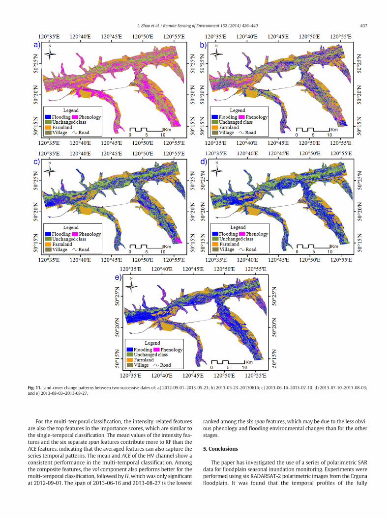
Fig. 11. Land-cover change patterns between two successive dates of: a) 2012-09-01–2013-05-23; b) 2013-05-23–20130616; c) 2013-06-16–2013-07-10; d) 2013-07-10–2013-08-03;and e) 2013-08-03–2013-08-27.

437L. Zhao et al. / Remote Sensing of Environment 152 (2014) 426–440

For the multi-temporal classification, the intensity-related featuresare also the top features in the importance scores, which are similar tothe single-temporal classification. The mean values of the intensity fea-tures and the six separate span features contribute more to RF than theACE features, indicating that the averaged features can also capture theseries temporal patterns. The mean and ACE of the HV channel show aconsistent performance in the multi-temporal classification. Amongthe composite features, the vol component also performs better for themulti-temporal classification, followed byH, whichwas only significantat 2012-09-01. The span of 2013-06-16 and 2013-08-27 is the lowest

ranked among the six span features, whichmay be due to the less obvi-ous phenology and flooding environmental changes than for the otherstages.

5. Conclusions

The paper has investigated the use of a series of polarimetric SARdata for floodplain seasonal inundation monitoring. Experiments wereperformed using six RADARSAT-2 polarimetric images from the Ergunafloodplain. It was found that the temporal profiles of the fully

Fig. 12. Class metrics for the trajectory analysis: a) PLAND; b) NLSI; c) IJI.

438 L. Zhao et al. / Remote Sensing of Environment 152 (2014) 426–440

polarimetric observations can reveal the seasonal fluctuations in scat-tering properties. In particular, composite polarimetric features can en-hance the understanding of the interaction between radar signals andland-cover types at the different seasons. The classification resultsshowed a high variability and indicate that it is difficult to find an opti-mum date for land-cover mapping of a floodplain, because the changesin the environmental factors significantly affect the land-cover types'separability. Multi-temporal information is therefore recommendedfor reliable floodplain interpretation. The vegetation pattern and hydro-period maps from the multi-temporal data allowed a reliable interpre-tation of the hydrological regime of the Erguna floodplain. Theperformances of the polarimetric observations for scattering mecha-nism interpretation and land-cover mapping were, however, different.The importance scores from the RF algorithm showed that theintensity-related observations performed better than the compositefeatures in both the single- and multi-temporal land-cover mapping.The intensity of the HV channel, in particular, was found to be the bestclassification predictor for the floodplain. In terms of the composite po-larimetric features, the volume scattering component has a relativelyhigher importance score, followed by H, γ, α, and the dbl component,the contributions of which depend on the characteristics of the land-cover types at the different phases. This highlights the importance ofquad-polarimetric information for floodplain monitoring. An investiga-tion of the main factors causing the backscattering changes was

performed by trajectory analysis. The spatial and temporal patterns ofthe phenology-induced and flooding-induced changes were identifiedby class metric profiles, based on the aggregated classification results.At the early phenological stage, most of the “bi-temporal” changescould be explained by vegetation development, while during the rainyseason, the effect of flooding became significant.

This analysis and the results obtained provide a framework to usePolSAR images to further understand the spatial and temporal charac-teristics of a floodplain. The results of the seasonal dynamics couldalso serve as baseline information to monitor future long-term inunda-tion, vegetation patterns, or they could be used to help with the assim-ilation of observations and hydrological models. Human-inducedchanges will be considered in a long-term series analysis in our futurestudy. Given the future missions of the Sentinel-1 C-band satellite andthe Radarsat Constellation Mission, it will soon be possible to explorethe dynamic characteristics of floodplains over a larger area and ashorter repeat period.

Acknowledgement

Thisworkwas supported in part by the 863High Technology Programof China, under Grant 2011AA120404, the National Basic Research Pro-gram of China (973 Program) under Grant 2011CB707105, the PublicWelfare Project in Surveying, under grant 201412002, the National

Fig. 13. Importance scores of the polarimetric features for the Erguna floodplain land-covermapping of: a) 2012-09-01; b) 2013-05-23; c) 2013-06-16; d) 2013-07-10; e) 2013-08-03; f)2013-08-27; and g) multi-temporal.

439L. Zhao et al. / Remote Sensing of Environment 152 (2014) 426–440

Natural Science Foundation of China, underGrant 61371199, and the Fun-damental Research Funds for the Central Universities, under grants2012619020213 and 2012619020206. The authors wish to thank the fol-lowing individuals: Jinqi Zhao andWeidong Sun fromWuhan University,Quan Chen and colleagues from RADI for the help in collecting data in thefield, and Erxue Chen from CAF for providing the RADARSAT-2 datasetsand for helping us with the processing of the LiDAR and CCD datasets.

Appendix A. Supplementary data

Supplementary data associated with this article can be found in theonline version, at http://dx.doi.org/10.1016/10.1016/j.rse.2014.06.026.These data include Google maps of the most important areas describedin this article.

References

Arnesen, A. S., Silva, T. S., Hess, L. L., Novo, E. M., Rudorff, C. M., Chapman, B.D., et al.(2013). Monitoring flood extent in the lower Amazon River floodplain using ALOS/PALSAR ScanSAR images. Remote Sensing of Environment, 130, 51–61.

Bayley, P. B. (1995). Understanding large river: Floodplain ecosystems. Bioscience, 45,153–158.

Bedient, P. B., Huber, W. C., Vieux, B. E., & Mallidu, M. (1988). Hydrology and floodplainanalysis (5th ed.). New Jersey: Prentice Hall.

Betbeder, J., Rapinel, S., Corpetti, T., Pottier, E., Corgne, S., & Moy, L. H. (2013). Multi-temporal classification of TerraSAR-X data for wetland vegetation mapping. Proc.SPIE 8887, Remote Sensing for Agriculture, Ecosystems, and Hydrology XV, 88871B,http://dx.doi.org/10.1117/12.2029092.

Bourgeau-Chavez, L. L., Leblon, B., Charbonneau, F., & Buckley, J. R. (2013). Evaluation ofpolarimetric Radarsat-2 SAR data for development of soil moisture retrieval algo-rithms over a chronosequence of black spruce boreal forests. Remote Sensing ofEnvironment, 132, 71–85.

Breiman, L. (2001). Random forests. Machine Learning, 45, 5–32.Cloude, S. R., & Pottier, E. (1997). An entropy based classification scheme for land applica-

tions of polarimetric SAR. IEEE Transactions on Geoscience and Remote Sensing, 35,68–78.

Costa, M. P., & Telmer, K. H. (2006). Utilizing SAR imagery and aquatic vegetation tomap fresh and brackish lakes in the Brazilian Pantanal wetland. Remote Sensing ofEnvironment, 105, 204–213.

Durden, S. L., Van Zyl, J. J., & Zebker, H. A. (1989). Modeling and observation of the radarpolarization signature of forested areas. IEEE Transactions on Geoscience and RemoteSensing, 27, 290–301.

ESA-Earth Online (2013). ESA declares end of mission for ENVISAT. https://earth.esa.int/web/guest/news/-/asset_publisher/G2mU/content/good-bye-e nvisat-and-thank-you

440 L. Zhao et al. / Remote Sensing of Environment 152 (2014) 426–440

Evans, T. L., Costa, M., Telmer, K., & Silva, T. S. (2010). Using ALOS/PALSAR andRADARSAT-2 to map land cover and seasonal inundation in the Brazilian Pantanal.IEEE Journal of Selected Topics in Applied Earth Observations and Remote Sensing, 3,560–575.

Frappart, F., Seyler, F., Martinez, J. -M., León, J. G., & Cazenave, A. (2005). Floodplain waterstorage in the Negro River basin estimated from microwave remote sensing of inun-dation area and water levels. Remote Sensing of Environment, 99, 387–399.

Friedman, J. H. (2001). Greedy function approximation: A gradient boosting machine.Annals of Statistics, 1189–1232.

Goroshko, O. A. (2007). Dauria international Chinese–Mongolian–Russian Protected Area:Results, perspectives, problems. Proceedings of the Status and Prospects of the Russian-Chinese Cooperation in Environment Conservation and Water Management, 27–28September, Moscow (pp. 260–264).

Grings, F. M., Ferrazzoli, P., Jacobo-Berlles, J. C., Karszenbaum, H., Tiffenberg, J., Pratolongo,P., et al. (2006). Monitoring flood condition in marshes using EMmodels and EnvisatASAR observations. IEEE Transactions on Geoscience and Remote Sensing, 44, 936–942.

Hajnsek, I., Papathanassiou, K., & Cloude, S. (2001). Removal of additive noise in polari-metric eigenvalue processing. Proceedings of the IEEE 2001 International Conferenceon Geoscience and Remote Sensing Symposium, IGARSS 2001, 9–13 July, Sydney(pp. 2778–2780).

Henderson, F. M., & Lewis, A. J. (2008). Radar detection of wetland ecosystems: A review.International Journal of Remote Sensing, 29, 5809–5835.

Hess, L. L., Melack, J. M., Filoso, S., & Wang, Y. (1995). Delineation of inundated area andvegetation along the Amazon floodplain with the SIR-C synthetic aperture radar.IEEE Transactions on Geoscience and Remote Sensing, 33, 896–904.

Hess, L. L., Melack, J. M., Novo, E. M., Barbosa, C. C., & Gastil, M. (2003). Dual-seasonmapping of wetland inundation and vegetation for the central Amazon basin.Remote Sensing of Environment, 87, 404–428.

Hess, L. L., Melack, J. M., & Simonett, D. S. (1990). Radar detection of flooding beneath theforest canopy: A review. International Journal of Remote Sensing, 11, 1313–1325.

Hong, S. -H., Wdowinski, S., Kim, S. -W., & Won, J. -S. (2010). Multi-temporal monitoringof wetland water levels in the Florida Everglades using interferometric syntheticaperture radar (InSAR). Remote Sensing of Environment, 114, 2436–2447.

Junk, W. J., Bayley, P. B., & Sparks, R. E. (1989). The flood pulse concept in river-floodplainsystems. Canadian Special Publication of Fisheries and Aquatic Sciences, 106, 110–127.

Kerr, P. C., Martyr, R. C., Donahue, A. S., Hope, M. E., Westerink, J. J., Luettich, R. A., et al.(2013). U.S. IOOS coastal and ocean modeling testbed: Evaluation of tide, wave,and hurricane surge response sensitivities to mesh resolution and friction in theGulf of Mexico. Journal of Geophysical Research: Oceans, 118, 4633–4661.

Kim, J. -W., Lu, Z., Lee, H., Shum, C., Swarzenski, C. M., Doyle, T.W., et al. (2009). Integratedanalysis of PALSAR/Radarsat-1 InSAR and ENVISAT altimeter data for mapping of ab-solute water level changes in Louisianawetlands. Remote Sensing of Environment, 113,2356–2365.

Kornelsen, K. C., & Coulibaly, P. (2013). Advances in soil moisture retrieval from syntheticaperture radar and hydrological applications. Journal of Hydrology, 476, 460–489.

Lang, M. W., Townsend, P. A., & Kasischke, E. S. (2008). Influence of incidence angle ondetecting flooded forests using C-HH synthetic aperture radar data. Remote Sensingof Environment, 112, 3898–3907.

Lee, J. S., Grunes, M. R., & de Grandi, G. (1999). Polarimetric SAR speckle filtering and itsimplication for classification. IEEE Transactions on Geoscience and Remote Sensing,37, 2363–2373.

Loosvelt, L., Peters, J., Skriver, H., De Baets, B., & Verhoest, N. E. C. (2012). Impact of reduc-ing polarimetric SAR input on the uncertainty of crop classifications based on theRandom Forests algorithm. IEEE Transactions on Geoscience and Remote Sensing, 50,4185–4200.

Loosvelt, L., Peters, J., Skriver, H., Lievens, H., Van Coillie, F. M. B., De Baets, B., et al. (2012).Random forests as a tool for estimating uncertainty at pixel-level in SAR image clas-sification. International Journal of Applied Earth Observation and Geoinformation, 19,173–184.

Lopez-Sanchez, J. M., Cloude, S. R., & Ballester-Berman, J.D. (2012). Rice phenologymonitoring by means of SAR polarimetry at X-band. IEEE Transactions on Geoscienceand Remote Sensing, 50, 2695–2709.

Manninen, T., Stenberg, P., Rautiainen, M., & Voipio, P. (2013). Leaf area index estimationof boreal and subarctic forests using VV/HH ENVISAT/ASAR data of various swaths.IEEE Transactions on Geoscience and Remote Sensing, 51, 3899–3909.

Marti-Cardona, B., Dolz-Ripolles, J., & Lopez-Martinez, C. (2013). Wetland inundationmonitoring by the synergistic use of ENVISAT/ASAR imagery and ancillary spatialdata. Remote Sensing of Environment, 139, 171–184.

Marti-Cardona, B., Lopez-Martinez, C., Dolz-Ripolles, J., & Bladè-Castellet, E. (2010). ASARpolarimetric, multi-incidence angle and multitemporal characterization of Doñanawetlands for flood extent monitoring. Remote Sensing of Environment, 114,2802–2815.

Martinez, J. -M., & Le Toan, T. (2007). Mapping of flood dynamics and spatial distributionof vegetation in the Amazon floodplain usingmultitemporal SAR data. Remote Sensingof Environment, 108, 209–223.

McGarigal, K., Cushman, S. A., & Ene, E. (2012). FRAGSTATS v4: Spatial pattern analysisprogram for categorical and continuous maps. Computer software program producedby the authors at the University of Massachusetts, Amherst (Available: http://www.umass.edu/landeco/research/fragstats/fragstats.html).

McNairn, H., Duguay, C., Brisco, B., & Pultz, T. J. (2002). The effect of soil and crop residuecharacteristics on polarimetric radar response. Remote Sensing of Environment, 80,308–320.

Mertens, B., & Lambin, E. F. (2000). Land‐cover‐change trajectories in southern Cameroon.Annals of the Association of American Geographers, 90, 467–494.

Mertes, L. A. (1997). Documentation and significance of the perirheic zone on inundatedfloodplains. Water Resources Research, 33, 1749–1762.

Moreau, S., & Le Toan, T. (2003). Biomass quantification of Andean wetland forages usingERS satellite SAR data for optimizing livestock management. Remote Sensing ofEnvironment, 84, 477–492.

Morena, L., James, K., & Beck, J. (2004). An introduction to the RADARSAT-2 mission.Canadian Journal of Remote Sensing, 30, 221–234.

Nghiem, S., Kwok, R., Yueh, S., & Drinkwater, M. (1995). Polarimetric signatures of seaice 2. Experimental observations. Journal of Geophysical Research, 100 (13681-13613,13698).

Ordoyne, C., & Friedl, M.A. (2008). Using MODIS data to characterize seasonal inundationpatterns in the Florida Everglades. Remote Sensing of Environment, 112, 4107–4119.

Petit, C., Scudder, T., & Lambin, E. (2001). Quantifying processes of land-cover change byremote sensing: Resettlement and rapid land-cover changes in south-easternZambia. International Journal of Remote Sensing, 22, 3435–3456.

Poncos, V., Teleaga, D., Bondar, C., & Oaie, G. (2013). A new insight on the water leveldynamics of the Danube Delta using a high spatial density of SAR measurements.Journal of Hydrology, 482, 79–91.

Pope, K. O., Rejmankova, E., Paris, J. F., & Woodruff, R. (1997). Detecting seasonal floodingcycles in marshes of the Yucatan Peninsula with SIR-C polarimetric radar imagery.Remote Sensing of Environment, 59, 157–166.

Pulvirenti, L., Chini, M., Pierdicca, N., Guerriero, L., & Ferrazzoli, P. (2011). Flood mon-itoring using multi-temporal COSMO-SkyMed data: Image segmentation andsignature interpretation. Remote Sensing of Environment, 115, 990–1002.

Quegan, S., Le Toan, T., Yu, J. J., Ribbes, F., & Floury, N. (2000). Multitemporal ERS SAR anal-ysis applied to forest mapping. IEEE Transactions on Geoscience and Remote Sensing,38, 741–753.

RwB–Rivers without Boundaries Coalition (2011). Protected areas and endangered spe-cies in Argun River Valley. Available: http://www.dauriarivers.org/maps/birds/

Schmitt, A., & Brisco, B. (2013). Wetland monitoring using the curvelet-based change de-tection method on polarimetric SAR Imagery. Water, 5, 1036–1051.

Touzi, R., Deschamps, A., & Rother, G. (2007). Wetland characterization using polarimetricRADARSAT-2 capability. Canadian Journal of Remote Sensing, 33, S56–S67.

Touzi, R., Deschamps, A., & Rother, G. (2009). Phase of target scattering for wetlandcharacterization using polarimetric C-band SAR. IEEE Transactions on Geoscience andRemote Sensing, 47, 3241–3261.

Townsend, P. A. (2001). Mapping seasonal flooding in forested wetlands usingmulti-temporal Radarsat SAR. Photogrammetric Engineering and Remote Sensing, 67,857–864.

Töyrä, J., & Pietroniro, A. (2005). Towards operational monitoring of a northern wetlandusing geomatics-based techniques. Remote Sensing of Environment, 97, 174–191.

Turkar, V., Deo, R., Rao, Y. S., Mohan, S., & Das, A. (2012). Classification accuracy of multi-frequency and multi-polarization SAR images for various land covers. IEEE Journal ofSelected Topics in Applied Earth Observations and Remote Sensing, 5, 936–941.

UNDP–United Nations Development Programme (2013). Strengthening the managementeffectiveness of the protected area network in the Daxing'anling landscape protection.(http://www.undp.org/content/dam/undp/documents/projects/CHN/Signed%20IP-82496-DaxingAnling.pdf).

van Zyl, J. J., & Kim, Y. (2011). Synthetic aperture radar polarimetry.New Jersey: JohnWiley& Sons.

Wang, Y., Hess, L. L., Filoso, S., &Melack, J. M. (1995). Understanding the radar backscatteringfrom flooded and nonflooded Amazonian forests: Results from canopy backscattermodeling. Remote Sensing of Environment, 54, 324–332.

Ward, D. P., Petty, A., Setterfield, S. A., Douglas, M. M., Ferdinands, K., Hamilton, S. K., et al.(2014). Floodplain inundation and vegetation dynamics in the Alligator Rivers region(Kakadu) of northern Australia assessed using optical and radar remote sensing.Remote Sensing of Environment, 147, 43–55.

Yajima, Y., Yamaguchi, Y., Sato, R., Yamada, H., & Boerner, W. -M. (2008). PolSAR imageanalysis of wetlands using a modified four-component scattering power decomposi-tion. IEEE Transactions on Geoscience and Remote Sensing, 46, 1667–1673.

Yamaguchi, Y., Moriyama, T., Ishido, M., & Yamada, H. (2005). Four-component scatteringmodel for polarimetric SAR image decomposition. IEEE Transactions on Geoscience andRemote Sensing, 43, 1699–1706.

Zhao, X., Stein, A., & Chen, X. -L. (2011). Monitoring the dynamics of wetland inundationby random sets on multi-temporal images. Remote Sensing of Environment, 115,2390–2401.

Zhao, L., Yang, J., Li, P., & Zhang, L. (2014). Characteristics analysis and classification ofcrop harvest patterns by exploiting high-frequency multi-polarization SAR Data.IEEE Journal of Selected Topics in Applied Earth Observations and Remote Sensing,http://dx.doi.org/10.1109/JSTARS.2014.2308273.

Zhao, L., Yang, J., Li, P., Zhang, L., Shi, L., & Lang, F. (2013). Damage assessment inurban areas using post-earthquake airborne PolSAR imagery. InternationalJournal of Remote Sensing, 34, 8952–8966.

Zhou, Q., Li, B., & Kurban, A. (2008a). Spatial pattern analysis of land cover changetrajectories in Tarim Basin, northwest China. International Journal of RemoteSensing, 29, 5495–5509.

Zhou, Q., Li, B., & Kurban, A. (2008b). Trajectory analysis of land cover change in aridenvironment of China. International Journal of Remote Sensing, 29, 1093–1107.