Remote Sensing of Environment 155 (2014) 210–221

Contents lists available at ScienceDirect

Remote Sensing of Environment

j ourna l homepage: www.e lsev ie r .com/ locate / rse

Evaluation of the SMAP brightness temperature downscaling algorithmusing active–passive microwave observations

Xiaoling Wu a,⁎, Jeffrey P. Walker a, Narendra N. Das b, Rocco Panciera c, Christoph Rüdiger a

a Department of Civil Engineering, Monash University, 3800, Australiab Jet Propulsion Laboratory (NASA), California Institute of Technology, CA 91109, USAc Cooperative Research Centre for Spatial Information, The University of Melbourne, 3053, Australia

⁎ Corresponding author at: Department of Civil EnginClayton Campus, Monash University, 3800 VIC, Australia.

E-mail address: xiaoling.wu@monash.edu (X. Wu).

http://dx.doi.org/10.1016/j.rse.2014.08.0210034-4257/© 2014 Elsevier Inc. All rights reserved.

a b s t r a c t

a r t i c l e i n f o

Article history:Received 22 October 2013Received in revised form 15 August 2014Accepted 15 August 2014Available online 20 September 2014

Keywords:DownscalingBrightness temperatureBackscatterActive–passiveSMAPSMAPEx

The baseline radiometer brightness temperature (Tb) downscaling algorithm for NASA's Soil Moisture ActivePassive (SMAP) mission, scheduled for launch in January 2015, is tested using an airborne simulation of theSMAP data stream. The algorithm synergistically uses 3 km Synthetic Aperture Radar (SAR) backscatter (σ) todownscale a 36 km radiometer Tb to 9 km. While the algorithm has already been tested using experimentaldatasets from field campaigns in the USA, it is imperative that it is tested for a comprehensive range of landsurface conditions (i.e. in different hydro-climatic regions) before global application. Consequently, this studyevaluates the algorithm using data collected from the Soil Moisture Active Passive Experiments (SMAPEx) insouth-eastern Australia, that closely simulate the SMAP data stream for a single SMAP radiometer pixel over a3-week interval, with repeat coverage every 2–3 days. The results suggest that the average root-mean-squareerror (RMSE) in downscaled Tb is 3.1 K and 2.6 K for h- and v-polarizations respectively, when downscaled to9 kmresolution. This increases to 8.2K and6.6 Kwhen applied at 1 kmresolution. Downscaling over the relativelyhomogeneous grassland areas resulted in 2 K lower RMSE than for the heterogeneous cropping area. Overall, thedownscaling error was around 2.4 K when applied at 9 km resolution for five of the nine days, which meets the2.4 K error target of the SMAP mission.

© 2014 Elsevier Inc. All rights reserved.

1. Introduction

Soil moisture is of great importance to global water cyclemonitoringand prediction, especially in agriculture, hydrology and meteorology(Seneviratne et al., 2010; Wagner et al., 2003). With the developmentof remote sensing technology (Jackson, Hsu, & O'Neill, 2002; Wagneret al., 2007), globalmapping of soil moisture from satellites is becominga viable alternative to traditional monitoring of soil moisture by in situnetworks of stations (Hain, Crow, Mecikalski, Anderson, & Holmes,2011). Consequently, methods are being developed to make use ofthis emerging soil moisture information to constrain numerical modelprediction of soil moisture, and hence improve the forecasting ofweather and floods (Albergel et al., 2010; Draper, Mahfouf, & Walker,2011; Houser, De Lannoy, & Walker, 2012; Reichle, Walker, Koster, &Houser, 2002), leading to significant societal benefits.

Over the past decade, passive microwave remote sensing hasemerged as the most promising approach for soil moisture mapping,due to its stronger and more direct connection between the observedbrightness temperature (Tb) and the near surface soil moisture (top

eering, Room 156/Building 60,Tel.: +61 3 9905 4957.

5 cm), than with active microwave sensing (radar backscatter) or ther-mal data (Kerr, 2007). The best results were found at low frequency(~1.4 GHz), due to the reduced effects by the atmosphere, surfaceroughness, vegetation attenuation, and increased observation depth.

The Soil Moisture and Ocean Salinity (SMOS) mission (Kerr et al.,2001) is the first satellite mission dedicated to soil moisture measure-ment using L-band passive microwave observations, launched bythe European Space Agency in 2009. Despite its high sensitivity tonear-surface soil moisture, radiometer technology suffers from havinga relatively low spatial resolution of approximately 40 km, due to limi-tations on the maximum antenna size that can be operated in space.Conversely, active microwave observations, which are more difficultto be interpreted for soil moisture content due to the confoundingeffects of vegetation and surface roughness, have a much finer spatialresolution (b3 km). Therefore, NASA is developing the Soil MoistureActive Passive (SMAP) mission (Entekhabi et al., 2010) scheduled forlaunch in January 2015 that will take advantage of the synergy betweenactive and passive observations. Accordingly, Das, Entekhabi, and Njoku(2011) have developed a baseline algorithm to overcome the individuallimitations of satellite-based L-band radiometer and radar observations.

This baseline algorithmdownscales the coarse scale brightness tem-peratures using the finer resolution radar backscatter cross-sections.The final soil moisture product is then retrieved from the downscaled

211X. Wu et al. / Remote Sensing of Environment 155 (2014) 210–221

brightness temperature at 9 km spatial resolution, which is deemedsuitable for hydro-meteorological applications such as flood predictionand agricultural activities (Albertson & Parlange, 1999; Weaver &Avissar, 2001). The algorithm has been tested with airborne field cam-paign data collected by the Passive and Active L-band System (PALS)instrument over various regions of the Continental United States(Das et al., 2011, 2014). However, more extensive testing of thealgorithm over different land covers and hydro-climatic regimes isimperative before application to the global SMAP data stream. Thetarget accuracy of this brightness temperature downscaling algorithmis 2.4 K as explicitly stated in the SMAP Algorithm Theoretical BasisDocument (ATBD, Entekhabi, Das, Njoku, Johnson, & Shi, 2012).

Other downscaling approaches have been studied using syntheticactive and passive observations, such as theBayesianmerging algorithm(Zhan, Houser, Walker, & Crow, 2006), which uses an inherentlydifferent strategy, resulting in a downscaled soil moisture product di-rectly through the synergy of the active and passive data in a Bayesianframework. However, such a technique has only been tested in anObservation System Simulation Experiment (OSSE) framework notwith real data. A further candidate downscaling approach is based onthe change detectionmethod, using the assumption of an approximatelylinear dependence of radar backscatter and brightness temperaturechange on soil moisture change (Narayan, Lakshmi, & Jackson, 2006;Piles, Entekhabi, & Camps, 2009). However, this downscaling algorithmhas limitations because of its operational implementation, and is notwell-tested using field campaign data.

In this study, the baseline brightness temperature downscalingmethod for the SMAP mission (Das et al., 2014), which is based on theassumption of a near-linear relationship between radar backscatter(σ) and radiometer brightness temperature (Tb), is tested usingairborne passive and active microwave observations collected over asemi-arid landscape during the SoilMoisture Active Passive Experiments(SMAPEx) conducted in Australia in 2010–2011, allowing assessment ofthe robustness of this baseline downscaling algorithmover different landconditions. The linear regression parameters are estimated using SMAP-type passive and active microwave data at 36 km resolution. These pa-rameters are then applied in the algorithm using aggregated radar dataat 3 km to derive downscaled passive microwave observations at 9 kmresolution, with the objective to evaluate the accuracy of the brightnesstemperature downscaling method. Although the ultimate objective ofthe SMAP mission is to produce a downscaled soil moisture product,this can only be achieved once the assumption that the baseline bright-ness temperature downscaling procedure is sufficiently accurate. Subse-quent to this, the standard and well-accepted passive microwave soilmoisture retrieval algorithms are applied. Therefore, the purpose ofthis paper is to challenge the baseline brightness temperature downscal-ing approach as proposed in the SMAP ATBD (Das et al., 2014; Entekhabiet al., 2012) and to test its robustness in terms of the downscaled bright-ness temperature values, according to the requirements set out in ATBD(Entekhabi et al., 2012). Testing of the final soil moisture retrieval accu-racy following the downscaling of the brightness temperature is outsidethe scope of this study.

2. Data set

The Soil Moisture Active Passive Experiments (Panciera et al., 2014)comprised a series of three campaigns undertaken over a one-year timeframe (winter July 5–10, 2010; summer December 4–8, 2010; andspring September 5–23, 2011), and were specifically designed tocontribute to the development of radar and radiometer soil moistureretrieval algorithms for the SMAP mission. The SMAPEx study area,with a size of approximately 38 km × 36 km, is situated within theMurrumbidgee River catchment (34.67°S, 35.01°S, 145.97°E, 146.36°E)as shown in Fig. 1. This site was chosen for testing the SMAP downscal-ing algorithm performance due to its flat topography, high density of

soil moisture monitoring stations, and spatial variability in soil, vegeta-tion and land use.

The SMAPEx area is characterized as semi-arid with a relatively flattopography, comprising of approximately 30% cropping area. The soiltypes are predominantly clays, red brown earths, and sand over clay,thus allowing an investigation of the downscaling algorithm underunique geophysical and meteorological conditions that are so far nottested for the downscaling algorithm. As shown in Fig. 1, the westernpart of the SMAPEx site is dominated by cropping areas, while the east-ern half consists mostly of grassland areas, including a large water bodyin the north-eastern quarter (approximately 500 m × 5 km in size).Some woodlands along the south-to-north flowing Yanco River, aswell as some small forest areas in the far East of the SMAPEx area, arealso present. This study site represents the heterogeneous land coverconditions that are typical of many landscapes, and thus requiredto evaluate the robustness of the SMAP active–passive baseline down-scaling algorithm performance.

The SMAPEx airborne instruments allowed the acquisition of con-current active and passive microwave remote sensing measurementsat 1.26 GHz and 1.41 GHz (L-band) frequencies respectively, beingthe same as the future SMAP sensors. Those data were collected by cov-ering an area the size of a SMAP radiometer footprint (approximately36 km × 38 km for the EASE grid at 35°S latitude) over a landscapetypical of south-eastern Australia, using a research aircraft. TheSMAPex airborne instrument suite consists of the Polarimetric L-bandMultibeam Radiometer (PLMR) and the Polarimetric L-band ImagingSynthetic Aperture Radar (PLIS), which when used together on thesame aircraft can provide a SMAP-like data stream for developing andtesting of the algorithms applicable to the SMAP mission viewingconfiguration. The SMAPEx flights also mimicked a time series of SMAP-like observations with a 2–3 day revisit time. A complete description ofthe experiment design can be found in Panciera et al. (2014).

In order to closely replicate the prototype SMAP data stream for de-velopment and testing of the downscaling techniques, data collectedduring the SMAPEx field campaigns were processed in terms of resolu-tion aggregation (36 km for passive and 3 km for active) and incidence-angle normalization (to 40° reference angle), to be in line with thespatial resolutions of SMAP (Wu, Walker, Rüdiger, Panciera, & Gray, inpress). The accuracy of the simulated SMAP data stream used in thisstudy has been determined as comparable to the error budget of theSMAP data stream, which is approximately 1.0 dB for backscatter at3 km resolution and 1.3 K for brightness temperature at 36 km resolu-tion (Wu et al., in press). The original resolutions of the data sets are1 km for the PLMR brightness temperatures and 10–30 m for the PLISbackscatter. Since they have been upscaled to 36 km and 3 km respec-tively for the purpose of application, the PLIS data were also aggregatedto 1 km and9 km to evaluate the performance of the SMAPdownscalingalgorithm at different spatial resolutions, since the native resolution ofthe SMAP radar is actually 1 km. Moreover, the reference Tb data usedfor evaluation of the downscaling results come from the original 1 kmPLMR, and were therefore aggregated to resolutions of 3 km and 9 kmfor use as reference at a range of scales.

The radiometer and radar data used to test this baseline downscal-ing algorithm were from the third SMAPEx campaign (SMAPEx-3,September 5–23, 2011), which was conducted during the spring vege-tation growing season. This campaign was used since it comprisednine regional flights over a 3-week time period with the 2–3 day revisittime of SMAP. A sample of the simulated SMAP data stream used in thisstudy is shown in Fig. 2.

3. Methodology

The baseline downscaling algorithm (Das et al., 2014) to be imple-mented for the SMAP mission aims to merge coarse resolution L-bandpassivemicrowave brightness temperature (Tb, in Kelvin)with fine res-olution L-band active microwave backscatter coefficient (σ, in decibel)

Fig. 1. Overview of the SMAPEx site showing the SMAP pixel sized study site, and the SMAP grid on which the 36 km resolution radiometer data, 3 km resolution radar data and 9 kmresolution active–passive downscaled product will be provided, together with area R in the north-eastern corner where the rainfall events happened during the third SMAPEx fieldcampaign.

212 X. Wu et al. / Remote Sensing of Environment 155 (2014) 210–221

based on the main assumption of a near-linear relationship betweenthem when observed at the same time, scale, and incidence angle. Thealgorithm is briefly described in the following paragraphs, while acomplete description is available in Das et al. (2014).

In the following the naming convention of ‘C’ (coarse), and ‘F’ (fine)represents the Tb and/or σ at 36 km and 3 km, respectively. Implemen-tation of this method requires a background Tb at C resolution, with thevariation of Tb imposed by the distribution of fine scale σ within Cmodulated by β(C) using the linear regression between Tb and σ at Cresolution according to:

Tbp F j

� �¼ Tbp Cð Þ þ β Cð Þ

� σpp F j

� �−σpp Cð Þ

h iþ Γ� σpq

Cð Þ−σpqF j

� �h in o: ð1Þ

where p indicates the polarization, includingh- and v-pol; and ppmeansco-polarization of radar observations σ, including hh or vv-pol. Correla-tions between four different combinations of Tbp and σpp have been

Fig. 2. Example of the simulated SMAP prototype data from PLMR and PLIS observations acro(a) backscatter (σ) at vv-polarization and at 3 km resolution aggregated from PLIS; (b) bright(c) Tb at v-polarization and at 3 km resolution aggregated from PLMR; (d) Tb at v-polarization

analyzed and will be presented in this paper. Tbp(Fj) is the brightnesstemperature value of a particular pixel “j” of resolution F, and σpp(Fj)is the corresponding radar backscatter value of pixel “j”. In this studythe value for σpp(C) (in the unit of dB) was obtained by aggregating10 m resolution PLIS data (in power units) within the coarse footprintC, with Tbp(C) aggregated from 1 km resolution PLMR observations(in Kelvin). Consequently, β(C), which depends on vegetation coverand type as well as surface roughness, is assumed to be time-invariantandhomogenous over the entire 36 km pixel and that it can be obtainedthrough the time-series of Tbp(C) and σpp(C). Since the radar also pro-vides high-resolution cross-polarization (hv-pol) backscatter measure-ments at resolution F, which is mainly sensitive to vegetation andsurface roughness, the sub-grid heterogeneity of vegetation/surfacecharacteristics within resolution C can be captured as [σpq(C) −σpq(Fj)] by the radar, where pq represents hv-pol. This heterogeneity in-dicator is then converted to variations in co-polarization pp backscatterby multiplying a sensitivity parameter Γ for each particular grid cell Cand season defined as Γ = [δσpp(Fj) / δσpq(Fj)]C. In other words, the

ss 9 days of SMAPEx-3 experiment (D1 to D9), with incidence angle normalized to 40°:ness temperature (Tb) at v-polarization and at 36 km resolution aggregated from PLMR;and at 9 km resolution aggregated from PLMR.

213X. Wu et al. / Remote Sensing of Environment 155 (2014) 210–221

Fig. 3. (a) Correlation between brightness temperature (Tb) and backscatter (σ) at different polarizations as shown, and spatial distribution of average Radar Vegetation Index (RVI) acrossthe 9 days (both correlation coefficient and RVI are displayed on a scale from 0 to 1) at 3 km spatial resolution; (b) plot of these correlation coefficients between Tb and σ at different po-larizations according to RVI.

214 X. Wu et al. / Remote Sensing of Environment 155 (2014) 210–221

term Γ × [σpq(C) − σpq(Fj)] can be described as the projection of thecross-polarization sub-grid heterogeneity onto the co-polarizationspace, thus converting the information of vegetation and surface charac-teristics to the variation of co-polarization backscatter. This term isconverted to brightness temperature through multiplication by β(C)in Eq. (1).

Using Eq. (1) in this study, the 36 km resolution Tb is downscaled to3 km resolution. The Tb at the intermediate resolution, i.e. 9 km, can beobtained by twomethods: i) directly upscaling the 3 kmdownscaled Tbto 9 km through linear aggregation; or ii) first averaging the backscatterdata (in power unit) from 3 km to 9 km, and subsequently using it inplace of the fine resolution backscatter data in Eq. (1). Both methodsare assessed in this paper. Moreover, due to the high resolution back-scatter provided by the SMAPEx airborne instruments, the 36 km reso-lution Tb can be downscaled to 1 km resolution using 1 km resolution σ,thus assessing the skill of this downscaling algorithm at three differentscales: 1 km, 3 km and 9 km.

The downscaled Tb at fine resolution is heavily dependent on thequality of the overall radiometer data at coarse scale, the relative back-scatter difference within the coarse grid, and the relationship with Tb asrepresented by the regression slope that is added to the backgroundvalue. The performance of the downscaling algorithm at different reso-lutions is evaluated by comparing the downscaled Tbwith the PLMR Tbdata at 1 km, 3 km and 9 km resolutions (aggregated from its original1 km resolution), respectively, in order to assess themerit of this down-scaling method in preparation for SMAP.

4. Results

4.1. Robustness of the linear active–passive relationship

The robustness of the linear relationship between Tb and σ is testedin this section for the six possible polarization combinations (i.e. Tbh andσhh, Tbv and σhh, Tbh and σvv, Tbv and σvv, Tbh and σhv, Tbv and σhv),aiming to determine the best combination for estimating the parameterβ. Consequently, the brightness temperature and backscatter observa-tions from PLMR and PLIS were spatially aggregated to 3 km resolution,resulting in a total of 144 pixelswithin the study area, presenting differ-ent levels of vegetation heterogeneity. Examples of those data areshown in Fig. 2(a) and (c).

The correlation coefficient R2, used to quantify the correlation be-tween Tb and σ for each 3 km pixel, was calculated using the entiretime series of Tb and σ of each individual pixel. Results for the differentpolarization combinations are shown in Fig. 3. Out of those, σ atvv-polarization showed the best correlation with Tb at both h- and v-polarizations; these results are in good agreementwith those presentedinDas et al. (2011). Therefore, the relationships ofσvv and Tbvwere usedto estimate β at v-pol, while σvv and Tbh were used to estimate β ath-pol, thus retrieving the downscaled Tb at h- and v-pol, respectively.

The influence of vegetation conditions on the correlation between Tband σ was also investigated. The Radar Vegetation Index (RVI) wasintroduced as an indicator of the compound vegetation conditions(including vegetation water content, vegetation biomass), which canbe obtained directly from the radar observations using the differentpolarizations by

RVI ¼ 8� σhv= σvv þ σhh þ 2� σhvð Þ; ð2Þ

where the radar backscatter values are in units of power (Kim& van Zyl,2009). Fig. 3 shows the average RVI values in each 3 km pixel calculatedfrom the 9 days of radar observations aggregated to 3 km, in order tocharacterize the vegetation conditions. This was done assuming thatvegetation conditions (and thus their associated RVI values) did notchange significantly across the 3-week period. For this experiment,the standard deviation (in time) of the RVI was found to be less than0.1 across the entire study area.

While the R2 between Tb and σ was generally larger in the westerntwo thirds than in the east of the SMAPEx area, the values of RVI weresmaller in the west than in the east. Although it was expected that thehighest correlation would be for low vegetation areas, the reason forthe higher RVI in the east is due to some small forests in the area andtrees along the Yanco River (see Fig. 3). This indicates that the down-scaling algorithm performance will be poorer in areas with denservegetation.

The sensitivity of Tb to changes in σ was analyzed using the slopeof the linear regression (parameter β) as a measure of quality. The rela-tionship between β and RVI is displayed in Figs. 4 and 5, with Fig. 4showing the relationship between Tbv and σvv anomalies under differ-ent vegetation conditions (i.e. different RVIs), and the sensitivity param-eter β estimated from observations of Tbv and σvv within the entire

Fig. 4. Relationship between brightness temperature at v-polarization (Tbv) and backscatter anomalies at vv-polarization (σvv) at 3 km resolution, for different vegetation characteristicsaccording to the Radar Vegetation Index (RVI) calculated from 3 km radar observations.

215X. Wu et al. / Remote Sensing of Environment 155 (2014) 210–221

study area. Both RVI and β were aggregated to 3 km resolution. Thesescatter plots show that: 1) Tbv and σvv have a near-linear relationship;2) the magnitude of β reduces as vegetation density increases, indicat-ing that the sensitivity of brightness temperature to backscatter de-creases, thus showing the dependence of sensitivity on the vegetationdensity. Fig. 5 shows the parameter β and its associated standard devi-ation plotted as a function of the RVI. The standard deviation of β esti-mation is higher at the RVI extremes, mainly due to the limited countsof Tb and σ pairs for those values. According to the numbers of pointsin each plot, most of the points are within the range of RVI from 0.3 to0.6, indicating that vegetation with RVI 0.3–0.6 dominates this studyarea. Investigation of the relationship between RVI and the accuracy ofthe downscaling algorithm for a specific area is out of the scope of this

Fig. 5. Dependency of regression parameter β (a) and associated standard deviation (b) of estimizations was estimated using backscatter (σ) at vv-polarization for brightness temperature (Tb

study, butwill possibly provide a directmethod of estimating the down-scaling performance globally from SMAP radar observations.

Given that σvv showed the best correlation with Tbv, the sensitivityparameter β for performing the downscaling in this study has been es-timated based on the combination of Tbv and σvv. In this particulardownscaling algorithm, βwas estimated from Tb andσ data both aggre-gated to 36 km resolution, in order to align with the resolutions ofSMAP. As a result, using the 9-days' time series of aggregated Tbv andσvv, β over the entire area has been estimated as approximately−2.2 K/dB, with the average RVI across the whole area being around0.5, aligning with the correlation between β and RVI as shown inFigs. 4 and 5. The same approach was applied to estimate β using Tbhand σvv, for the downscaling of Tb at h-pol. In this case, similar trends

ation from the Radar Vegetation Index (RVI) at 3 km resolution. The β at h- and v-polar-) at h- and v-polarizations.

216 X. Wu et al. / Remote Sensing of Environment 155 (2014) 210–221

for β estimation and its standard error were found with respect to RVI,as shown in Fig. 5. However, the magnitude of β at different RVIs is onaverage 1.2 K/dB higher than that estimated from Tbv and σvv, implyingthat the sensitivity of Tbh to σvv is higher than the sensitivity of Tbv toσvv. Regardless of the actual variation of vegetation within the entirearea,βwas estimated as a single value across the 36 kmarea as outlinedin the SMAP baseline active–passive algorithm. Based on this prelimi-nary analysis of the relationship between RVI and β, it is suggestedthat a more detailed investigation of the spatial distribution of βwithinthe 36 km area should be undertaken, including an investigation of apotential spatially varying β implementation in the SMAP baselinealgorithm.

4.2. Estimation of Γ

The parameter Γ, i.e. the sensitivity of σvv to σhv, can be estimatedusing snapshots of σvv and σhv values at each pixel within a certainarea. Since radar backscatter σ at hv-pol is more related to the vegeta-tion canopy than to the soil, the distribution of σhv across the entirearea can be used to characterize the heterogeneity of vegetation condi-tions in that area. Therefore, downscaling results can be improved byincluding the influence of vegetation on the backscatter observation,by converting the σhv variation within the entire area to σvv variation,by multiplying with the sensitivity Γ.

In order to obtain an estimate for the parameter Γ, the study areawasdivided into 16 sub-areas of 9 kmby 9 km in size, and the value of Γwascalculated using the snapshots of all σvv–σhv pairs at 1 km resolutioncontainedwithin each of those sub-areas, allowing an analysis of the re-lationship between estimation of Γ and RVI. Accordingly, the day-to-dayvariation and average of Γ with respect to RVI are shown in Fig. 6, to-gether with an example of the distribution of Γ at each 9 km sub-areaacross the entire study area on Day 9 (23rd September, 2011). It isshown that for RVI values ranging from 0.4 to 0.9 the estimation of Γ issimilar, on the order of 0.45, while for RVI values less than 0.4, Γ ismuch higher, indicating that the sensitivity of σvv to σhv increases

Fig. 6. Estimation of parameter Γ: (a) Γ plotted as a function of the Radar Vegetation Index (RVI)over the entire study area on Day 9; each pixel has a size of 9 km × 9 km (low: 0.3; high: 0.6)

when the vegetation cover reduces. Again, larger standard deviationswere found for both extremes due to low counts of pixels.

4.3. Accuracy of downscaling

According to the baseline approach the downscaled brightness tem-perature at fine resolution are a function of the background Tb valueplus a variation of Tb within the entire area derived from the variationof the backscatter from the mean. In this study, the background Tb istaken as the aggregated 36 km Tb from PLMR, and the variation of Tbat higher resolution is characterized by the variation ofσvv fromPLIS ob-servations, aggregated to the downscaling resolution. The influence ofvegetation is then deduced using σhv, due to its strong correlationwith vegetation conditions. Consequently, the downscaled Tb resultswere retrieved at resolutions of 1 km, 3 km and 9 km, either from aggre-gating the 1 km resolution downscaled Tb to 3 km and 9 km resolutionrespectively, or from first aggregating the 1 km resolution radar obser-vations to 3 km and 9 km before using them to disaggregate the36 km Tb. Both methods were applied and showed similar results;results shown in this paper are based on the former method. Prior toapplying the downscaling algorithm, the main water body in the farnorth-eastern section of the area, and some irrigated cropping areaswithin the western part of the regional area, were removed (theseareas collectively represented approximately 1% of the entire studyregion) to reduce the influence of surface water on the resulting down-scaling accuracy.

Based on the estimation of β at h- and v-polarizations and the day today matrix of Γ estimates derived in the previous sections, the baselinedownscaling algorithm performance was evaluated for each of the ninedays of SMAPEx airborne acquisitions. In order to analyze the influenceof vegetation characteristics on the resulting downscaled Tb, the down-scaling algorithm was applied in two scenarios: in scenario “A1”, thevegetation heterogeneity across the study area was ignored; in scenario“A2”, the vegetation heterogeneity across the study area was taken intoaccount. In otherwords, A1was characterized by setting Γ=0,while A2

on different days; (b) standard deviation of Γ estimation; and (c) example of Γ distribution.

Table 1Accuracy of the SMAP baseline downscaling algorithm. Root mean square error (RMSE) between downscaled brightness temperature (Tb) and reference Tb is shown for the entire studyarea across the 9-days (D1 to D9) with respect to polarization and resolution of the final downscaled product; results based on scenario A1 (Γ = 0) and scenario A2 (Γ ≠ 0) are shown.

Downscalingresolution (km)

D1 D2` D3 D4 D5 D6 D7 D8 D9 Average

h v h v h v h v h v h v h v h v h v h v

1 A1 11.7 9.1 10.4 8.2 10.5 7.9 10.6 8.3 9.1 6.8 9.0 6.7 8.1 6.0 8.4 6.2 8.2 5.8 9.5 7.2A2 10.5 8.4 9.5 8.0 9.0 7.1 9.2 8.0 8.1 6.2 8.1 6.1 6.3 5.2 7.0 5.6 6.6 5.1 8.2 6.6

3 A1 9.1 7.0 7.7 6.1 7.6 5.6 7.6 5.9 5.8 4.4 6.2 4.3 5.1 3.6 5.4 3.8 5.2 3.6 6.6 4.9A2 8.6 6.7 7.3 6.0 5.6 4.6 6.8 5.5 4.9 4.2 5.2 4.1 4.2 3.3 4.2 3.3 3.3 3.2 5.5 4.5

9 A1 6.0 4.7 4.7 3.9 4.9 3.5 4.9 3.8 3.2 2.5 3.3 2.4 2.5 1.8 3.2 2.2 2.9 1.8 3.9 2.9A2 5.8 4.5 4.6 3.7 3.9 3.1 4.0 3.5 2.5 2.4 2.4 2.1 1.5 1.5 2.0 1.7 1.9 1.5 3.1 2.6

217X. Wu et al. / Remote Sensing of Environment 155 (2014) 210–221

used Γ≠ 0 in Eq. (1). In the following, the results of the downscaling arecompared among the two scenarios.

Downscaling results on each day of SMAPEx-3 are shown in Table 1for different resolutions and polarizations. It is noted from Table 1 thatthe downscaled results at v-polarization had relatively lower RMSEthan those at h-polarization, likely due to thebetter correlation betweenσvv and Tbv than between σvv and Tbh. Moreover, there is an obviousreduction of RMSE at both polarizations when applied to a largerscale, e.g. from 1 km to 3 km and 9 km respectively, which can beattributed to the reduction of random (white) noise following theaggregation of the backscatter data.

Apart from resolution and polarization, the RMSE was furtherreduced when taking into account the variation of vegetation acrossthe entire area, confirming that the Γ term in Eq. (1) can be used to com-pensate the influence of vegetation conditions to some degree, thusyielding a more accurate finer resolution brightness temperatureproduct. Quantitative results are provided in Table 1, showing thatthe average RMSE of the 9 days at v-polarization was lower by 1–2 Kthan ath-polarization, and decreased by approximately 5 Kwhen aggre-gating from 1 km to 9 km. As before, after considering the influence ofvegetation heterogeneity (scenario A2 with Γ≠ 0), the RMSE of down-scaled Tb had an improvement of 1.2 K at h-polarization and 0.5 K atv-polarization over the results based on the assumption of a homoge-neous vegetation (scenario A1, Γ = 0). Moreover, during 5 out of9 days the RMSE was found to be around 2.4 K at 9 km resolution,which is within the target error of the SMAP mission (2.4 K when thevegetation water content is less than 5 kg/m2), confirming that thebaseline downscaling algorithm has the potential to retrieve mediumresolution brightness temperature with an error of around 2.4 K overheterogeneous areas.

In order to confirm that the use of σvv is more efficient than σhh, assuggested by the correlation analysis between Tb and σ, an additionaltest was performed using coarse resolution Tb and fine resolution σhh

to retrieve Tb at scales of 1 km, 3 km and 9 km. The performance levelsof the algorithmusingσvv andσhh arepresented in Table 2, showing thatthe RMSE based on σvv is around 0.2 to 0.9 K lower than that based onσhh, confirming the results fromFig. 3where therewas a stronger corre-lation of σvv to Tb than σhh.

Examples of downscaled Tb maps are shown in Fig. 7 for Day 9 at1 km, 3 km and 9 km resolutions, alongside the reference data fromPLMR, and the pixel-by-pixel Tb difference between downscaled andreference values. It is noted that the downscaling errors are generallylarger in the western part of the study area than the central section,

Table 2Downscaling algorithm performance in terms of root mean square error (RMSE) whenusing backscatter at hh- and vv-polarizations, together with the RMSE difference betweenthese two polarizations.

Downscaling resolution (km) σvv σhh Difference

h v h v h v

1 8.2 6.6 9.1 7.2 −0.9 −0.63 5.5 4.5 6.2 5.0 −0.7 −0.59 3.1 2.6 3.3 3.3 −0.2 −0.2

which is mainly due to the western part being dominated by irrigatedand dry-land cropping areas, while the central area is largely coveredby grassland. A consequence of the large heterogeneity of the croppingareas was a relatively large RMSE in those areas, as highlighted bythe RMSE behavior from west to east of the entire region in Fig. 8.Dependence of RMSE for the 36 strips (each with 1 km width whenprogressing from west to east and having 36 km length in the north–south direction) covering the SMAPEx study area is displayed in Fig. 8.Overall, the RMSE of the central area, the dominantly grassland areabetween distances of 18 km and 28 km, is around 2 K lower thanelsewhere.

As shown in Figs. 3 to 5, β estimation should be lower than−3 K/dB(at v-pol) and −4 K/dB (at h-pol) in the western area and should behigher than −2 K/dB (at h- & v-pol) in the eastern area due to thevariation in RVI across the entire region. However, since the constantvalue of β from 36 km Tb and σ is used in this study, which is−2.2 K/dB(at v-pol) and −3.4 K/dB (at h-pol), there is an under-estimation inthe west and over-estimation in the east, which is directly related tothemagnitude of β variation from the nominal value used and thereforefurther influencing the accuracy of this downscaling algorithm. More-over, the RMSE in the east is relatively high, due to the influence fromthe large areas of woodland along the river which runs approximatelysouth to north in that part, and some other areas of dense forest.

A further evaluation of the skill of this particular downscaling algo-rithm was through the correlation between downscaled and referenceTb at 9 km resolution (Figs. 9 and 10). While these two black dashedlines represent RMSE less than 2.4 K (the SMAP target), the outer twoblack solid lines represent RMSE less than 4 K (the SMOS target). It isnoted from Figs. 9 and 10 that more than 93% of the points from D3(“D” represents “Day”) to D9 are within the SMOS target range, andfive of them (from D5 to D9) have more than 90% of points within theSMAP target range, showing that the baseline downscaling algorithmcan provide accurate Tb at 9 km.

Nonetheless, the results of the first days i.e. D1 to D4 displayed rela-tively poor performancewhen compared to the later days. In particular,D1 and D2 contain significant noise levels. One possible reason is attrib-uted to increased heterogeneity in near surface soil moisture due to theheavy rainfall events in the northeastern part of the study area at thebeginning of SMAPEx-3 as shown in Figs. 1 and 2(c), subsequentlyresulting in more heterogeneous radiometer and radar observations. Itis shown in Figs. 9 and 10 that D1 to D4 had a higher standard deviationof Tb (reference Tb) when compared to the other days. Since Tb is moresensitive to the immediate soil moisture changes due to the rain in thisregion, the value of Tb drop according to soil moisture increase is moresignificant than the radar backscatter changes, as the latter is more in-fluenced by the vegetation cover and consequently less sensitive tothe soil moisture changes. Consequently, the sensitivity of backscatterto Tb change decreases, resulting in an obvious difference in β for thearea subjected to rainfall when compared with the other drier areas,which would have dominated the derivation of the β value used. Thisis underlined by the RMSE in the north-eastern part (area R) of thestudy area being around 3 K higher than throughout the remainingarea (at 3 km resolution), impacting the overall large RMSE for thatday, as shown in Fig. 11. In addition, the average RVI of area R is ~0.56,

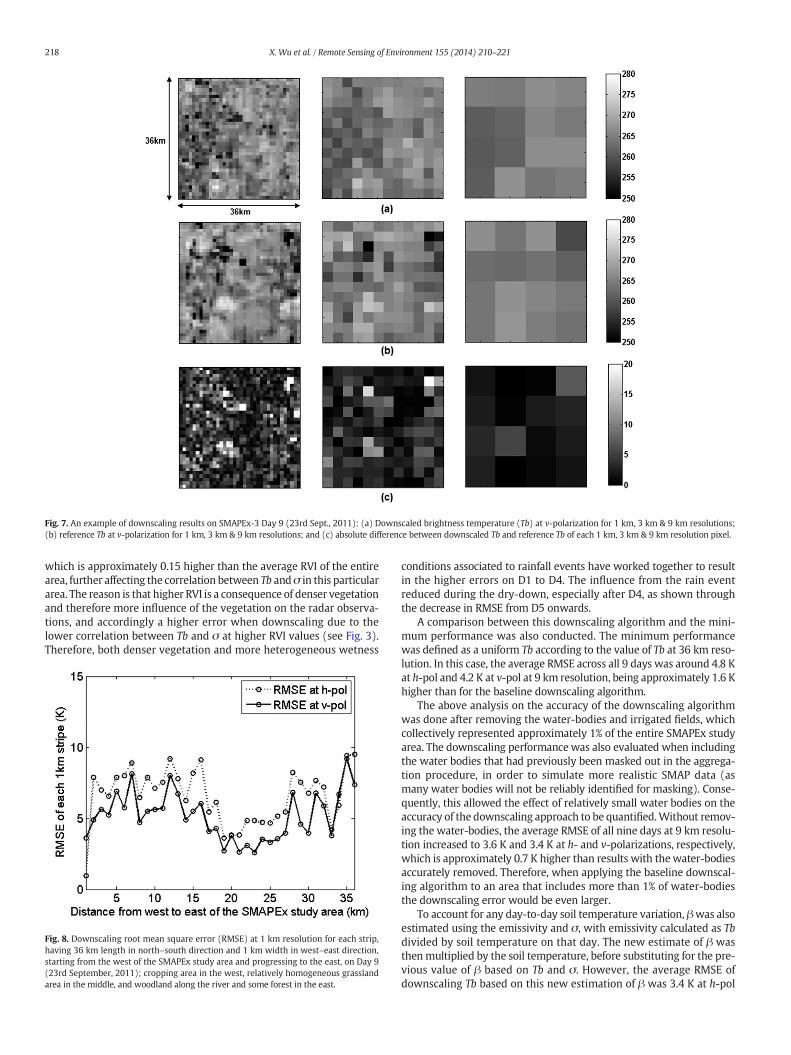
Fig. 7. An example of downscaling results on SMAPEx-3 Day 9 (23rd Sept., 2011): (a) Downscaled brightness temperature (Tb) at v-polarization for 1 km, 3 km & 9 km resolutions;(b) reference Tb at v-polarization for 1 km, 3 km & 9 km resolutions; and (c) absolute difference between downscaled Tb and reference Tb of each 1 km, 3 km & 9 km resolution pixel.

218 X. Wu et al. / Remote Sensing of Environment 155 (2014) 210–221

which is approximately 0.15 higher than the average RVI of the entirearea, further affecting the correlation between Tb andσ in this particulararea. The reason is that higher RVI is a consequence of denser vegetationand therefore more influence of the vegetation on the radar observa-tions, and accordingly a higher error when downscaling due to thelower correlation between Tb and σ at higher RVI values (see Fig. 3).Therefore, both denser vegetation and more heterogeneous wetness

Fig. 8. Downscaling root mean square error (RMSE) at 1 km resolution for each strip,having 36 km length in north–south direction and 1 km width in west–east direction,starting from the west of the SMAPEx study area and progressing to the east, on Day 9(23rd September, 2011); cropping area in the west, relatively homogeneous grasslandarea in the middle, and woodland along the river and some forest in the east.

conditions associated to rainfall events have worked together to resultin the higher errors on D1 to D4. The influence from the rain eventreduced during the dry-down, especially after D4, as shown throughthe decrease in RMSE from D5 onwards.

A comparison between this downscaling algorithm and the mini-mum performance was also conducted. The minimum performancewas defined as a uniform Tb according to the value of Tb at 36 km reso-lution. In this case, the average RMSE across all 9 days was around 4.8 Kat h-pol and 4.2 K at v-pol at 9 km resolution, being approximately 1.6 Khigher than for the baseline downscaling algorithm.

The above analysis on the accuracy of the downscaling algorithmwas done after removing the water-bodies and irrigated fields, whichcollectively represented approximately 1% of the entire SMAPEx studyarea. The downscaling performance was also evaluated when includingthe water bodies that had previously been masked out in the aggrega-tion procedure, in order to simulate more realistic SMAP data (asmany water bodies will not be reliably identified for masking). Conse-quently, this allowed the effect of relatively small water bodies on theaccuracy of the downscaling approach to be quantified.Without remov-ing the water-bodies, the average RMSE of all nine days at 9 km resolu-tion increased to 3.6 K and 3.4 K at h- and v-polarizations, respectively,which is approximately 0.7 K higher than results with thewater-bodiesaccurately removed. Therefore, when applying the baseline downscal-ing algorithm to an area that includes more than 1% of water-bodiesthe downscaling error would be even larger.

To account for any day-to-day soil temperature variation, βwas alsoestimated using the emissivity and σ, with emissivity calculated as Tbdivided by soil temperature on that day. The new estimate of β wasthenmultiplied by the soil temperature, before substituting for the pre-vious value of β based on Tb and σ. However, the average RMSE ofdownscaling Tb based on this new estimation of β was 3.4 K at h-pol

Fig. 9. Scatter plots of downscaled and reference brightness temperature (Tb) at 9 km resolution on each of SMAPEx-3 Day 1 to Day 9, at h-pol (open dots) and v-pol (solid dots); innerblack solid line: RMSE is 0 K; two black dashed lines: RMSE = 2.4 K (SMAP Tb target accuracy); outer two black solid lines: RMSE = 4 K (SMOS Tb target accuracy).

219X. Wu et al. / Remote Sensing of Environment 155 (2014) 210–221

and 2.7 K at v-pol at 9 km resolution, being only slightly different to pre-vious results.

4.4. Reliability of baseline downscaling algorithm

In this study, the accuracy of downscaling results was primarily de-termined by the parameter β as shown in Eq. (1). Themain limitation ofthe downscaling method introduced in Das et al. (2014) is the assump-tion of a constant β across the entire study area. The parameter β, usedto denote the sensitivity of Tb to σ, in reality varies with respect to theland surface conditions, as shown in Figs. 4 and 5. Therefore, the as-sumption of a constant value of β could not represent the real distribu-tion of β due to the heterogeneity of the study area. For example, if thestudy areawas entirely covered by homogenous grassland, then the useof a singleβwould bemore appropriate for use in downscaling. Howev-er, as shown in the above results, the variation on land cover typesacross the entire site, or soil moisture heterogeneity due to rainingevents in someparticular areas, or somewater-bodies, or surface rough-ness, or vegetation evolution due to different seasons would result indifferent values of β across the site.

As βwas estimated from time-series of Tb and σ at 36 km, more ac-curate regression could be obtained from a longer time period so as tomake it statistically significant. However, the vegetation and roughnessconditions are changing as time goes on, which will result in different βestimates through time. Therefore, a moving window of β estimationshould be adopted when applying the downscaling algorithm to along time period. This is not done in this study but should be acknowl-edged for future application.

5. Conclusions

The objective of this study was to test the robustness of the baselinedownscaling approach proposed for the SMAPmission, using a simulat-ed SMAP data stream from the SMAPEx field campaign in Australia. Theerrors associated with the downscaling algorithm were assessed forseveral resolutions of the final downscaled product and at both h- andv-polarizations. The average RMSE of downscaled Tb across 9 days at9 km resolution was 3.1 K and 2.6 K at h- and v-polarizations, which in-creased to 5.5 K and 4.5 K at 3 km resolution, and 8.2 K and 6.6 K at 1 kmresolution. The algorithmwas found to perform poorly in the early days

Fig. 10. Scatter plots of downscaled and reference brightness temperature (Tb) at 9 kmresolution for all SMAPEx-3 acquisitions (Day 1 to Day 9), at h-pol and v-pol. Solid dotsand stars represent data from SMAPEx-3Day 5 to Day 9,while the open dots and stars rep-resent data from SMAPEx-3 Day 1 to Day 4. Inner black solid line: RMSE is 0 K; two blackdashed lines: RMSE = 2.4 K (SMAP Tb target accuracy); outer black solid lines: RMSE =4 K (SMOS Tb target accuracy).

220 X. Wu et al. / Remote Sensing of Environment 155 (2014) 210–221

of the experiment due to large rainfall events in the study area that cre-ated a large spatial heterogeneity in terms of soil moisture content. Incontrast, the last 5 days of the experiment, characterized by a dryingdown period and no rainfall, showed an increase in the algorithmperformance, with an RMSE consistently better than 2.4 K at 9 kmresolution, indicating that the baseline downscaling algorithm has thepotential to fulfill the requirements of SMAP.

It was also shown that the accuracy of the downscaling approachwas primarily determined by the correlation between Tb and σ, whichwas in fact affected by the vegetation characteristics across the entirestudy area and the sensitivity of brightness temperature relative toradar backscatter (as quantified by the slope β of the linear regression).Moreover, it was found that σ at vv-polarization was best correlated toTb at both polarizations, therefore being more suitable for use in thedownscaling algorithm than σ at hh- and hv-polarizations. While a bet-ter estimation of β at 36 km scalemay be expected fromSMAP than thatachieved here, due to the relatively short nature of this experiment, theimpact from temporal changes would be an important consideration.

Fig. 11. Comparison between the root mean square error (RMSE) of the north-eastern(area “R”) of the SMAPEx study area, and RMSE of the entire study area. Calculations arefor 3 km resolution at both polarizations across 9 days.

Some preliminary results on the relationship between β and RVI,and the relationship between Γ and RVI have been discussed in thisstudy. They indicate that an improvement in the parameterization of βand Γ may be obtained through their correlation with RVI, allowing abetter retrieval and more accurate spatial distribution of β and Γ acrossthe entire area. In future studies it is also important to investigate theestimation of β and Γ at the pixel resolution with respect to landcover, vegetation water content, surface roughness etc., and how thesecan improve the accuracy of the downscaling algorithm by incorporat-ing this fine scale information into the downscaling approach.

Acknowledgments

The SMAPEx field campaigns and related research developmenthave been funded by the Australian Research Council Discovery(DP0984586) and Infrastructure (LE0453434 and LE0882509) grants.The authors acknowledge the collaboration of a large number of scien-tists from throughout Australia and around the world, and in particularkey personnel from the SMAP team which provided significant contri-butions to the campaign's design and execution. The authors also ac-knowledge the scholarships awarded by Monash University to supportXiaoling Wu's PhD research.

References

Albergel, C., Calvet, J. C., Mahfouf, J. F., Rüdiger, C., Barbu, A. L., Lafont, S., et al. (2010).Monitoring of water and carbon fluxes using a land data assimilation system: Acase study for southwestern France. Hydrology and Earth System Sciences, 14,1109–1124.

Albertson, J.D., & Parlange, M. B. (1999). Natural integration of scalar fluxes from complexterrain. Advances in Water Resources, 23, 239–252.

Das, N. N., Entekhabi, D., & Njoku, E. G. (2011). An algorithm for merging SMAP radiom-eter and radar data for high-resolution soil-moisture retrieval. IEEE Transactions onGeoscience and Remote Sensing, 49, 1504–1512.

Das, N. N., Entekhabi, D., Njoku, E. G., Shi, J. J. C., Johnson, J. T., & Colliander, A. (2014). Testsof the SMAP combined radar and radiometer algorithm using airborne field campaignobservations and simulated data. IEEE Transactions on Geoscience and Remote Sensing,52, 2018–2028.

Draper, C. S., Mahfouf, J. F., & Walker, J. P. (2011). Root zone soil moisture from the assim-ilation of screen-level variables and remotely sensed soil moisture. Journal ofGeophysical Research, [Atmospheres], 116, D02127.

Entekhabi, D., Das, N. N., Njoku, E. G., Johnson, J., & Shi, J. C. (2012). Algorithm theoreticalbasis document: L2 & L3 radar/radiometer soil moisture (active/passive) data prod-ucts. Initial Release, v. 1.

Entekhabi, D., Njoku, E. G., O'Neill, P. E., Kellogg, K. H., Crow, W. T., Edelstein, W. N., et al.(2010). The Soil Moisture Active Passive (SMAP) mission. Proceedings of the IEEE, 98,704–716.

Hain, C. R., Crow, W. T., Mecikalski, J. R., Anderson, M. C., & Holmes, T. (2011). An inter-comparison of available soil moisture estimates from thermal infrared and passivemicrowave remote sensing and land surface modeling. Journal of GeophysicalResearch, 116, D15107.

Houser, P. R., De Lannoy, G., & Walker, J. P. (2012). Hydrologic data assimilation. InTech.Jackson, T. J., Hsu, A. Y., & O'Neill, P. E. (2002). Surface soil moisture retrieval andmapping

using high-frequency microwave satellite observations in the southern great plains.Journal of Hydrometeorology, 3, 688–699.

Kerr, Y. (2007). Soil moisture from space: Where are we? Hydrogeology Journal, 15,117–120.

Kerr, Y. H., Waldteufel, P., Wigneron, J. P., Martinuzzi, J., Font, J., & Berger, M. (2001). Soilmoisture retrieval from space: the Soil Moisture and Ocean Salinity (SMOS) mission.IEEE Transactions on Geoscience and Remote Sensing, 39, 1729–1735.

Kim, Y., & van Zyl, J. (2009). A time-series approach to estimate soil moisture using polar-imetric radar data. IEEE Trans. Geosci. Remote Sens., 47, 2519–2527.

Narayan, U., Lakshmi, V., & Jackson, T. J. (2006). High-resolution change estimation of soilmoisture using L-band radiometer and radar observations made during the SMEX02experiments. IEEE Transactions on Geoscience and Remote Sensing, 44, 1545–1554.

Panciera, R., Walker, J. P., Jackson, T. J., Gray, D. A., Tanase, M.A., Dongryeol, R., et al.(2014). The Soil Moisture Active Passive Experiments (SMAPEx): Toward soilmoisture retrieval from the SMAP mission. IEEE Transactions on Geoscience andRemote Sensing, 52, 490–507.

Piles, M., Entekhabi, D., & Camps, A. (2009). A change detection algorithm for retrievinghigh-resolution soil moisture from SMAP radar and radiometer observations. IEEETransactions on Geoscience and Remote Sensing, 47, 4125–4131.

Reichle, R. H., Walker, J. P., Koster, R. D., & Houser, P. R. (2002). Extended versus ensembleKalman filtering for land data assimilation. Journal of Hydrometeorology, 3, 728–740.

Seneviratne, S. I., Corti, T., Davin, E. L., Hirschi, M., Jaeger, E. B., Lehner, I., et al. (2010).Investigating soil moisture–climate interactions in a changing climate: A review.Earth-Science Reviews, 99, 125–161.

221X. Wu et al. / Remote Sensing of Environment 155 (2014) 210–221

Wagner, W., Blsch, G., Pampaloni, P., Valvet, J., Bizarri, B., Wigneron, J., et al. (2007).Operational readiness of microwave remote sensing of soil moisture for hydrologicapplications. Nordic Hydrology, 38, 1–20.

Wagner,W., Scipal, K., Pathe, C., Gerten, D., Lucht,W., & Rudolf, B. (2003). Evaluation of theagreement between the first global remotely sensed soil moisture data with modeland precipitation data. Journal of Geophysical Research, [Atmospheres], 108, 4611.

Weaver, C. P., & Avissar, R. (2001). Atmospheric disturbances caused by humanmodifica-tion of the landscape. Bulletin of the American Meteorological Society, 82, 269–281.

Wu, X., Walker, J. P., Rüdiger, C., Panciera, R., & Gray, D. (2014). Simulation of the SMAPdata stream from SMAPEx field campaigns in Australia. IEEE Transactions onGeoscience and Remote Sensing, 53, 1921–1934.

Zhan, X., Houser, P. R., Walker, J. P., & Crow, W. T. (2006). A method for retrievinghigh-resolution surface soil moisture from hydros L-band radiometer and radarobservation. IEEE Transactions on Geoscience and Remote Sensing, 44, 1534–1544.