Remote Sensing of Environment 151 (2014) 138–148

Contents lists available at ScienceDirect

Remote Sensing of Environment

j ourna l homepage: www.e lsev ie r .com/ locate / rse

Using the regression estimator with Landsat data to estimate proportionforest cover and net proportion deforestation in Gabon

Christophe Sannier a,⁎, Ronald E. McRoberts b, Louis-Vincent Fichet a, Etienne Massard K. Makaga c

a SIRS, Parc de la Cimaise, 27 rue du Carrousel, 59650 Villeneuve d'Ascq, Franceb Northern Research Station, U.S. Forest Service, Saint Paul, MN, USAc AGEOS, BP 546 Libreville, Gabon

⁎ Corresponding author.E-mail address: christophe.sannier@sirs-fr.com (C. San

0034-4257/$ – see front matter © 2013 Elsevier Inc. All rihttp://dx.doi.org/10.1016/j.rse.2013.09.015

a b s t r a c t

a r t i c l e i n f o

Article history:Received 16 November 2012Received in revised form 15 September 2013Accepted 17 September 2013Available online 10 October 2013

Keywords:REDDTwo-stage estimation

Forest cover maps were produced for the Gabonese Agency for Space Studies and Observations (AGEOS) for1990, 2000 and 2010 for an area of approximately 102,000 km2 corresponding to 38% of the total area ofGabon and representative of the range of human pressure on forest resources. The maps were constructedusing a combination of a semi-automated classification procedure and manual enhancements to ensure thegreatest possible accuracy. A two-stage area frame sampling approach was adopted to collect reference datafor assessing the accuracy of the forest cover maps and to estimate proportion forest cover and net proportiondeforestation. A total of 251 2 × 2 km segments or primary sample units (PSUs) were visually interpreted by ateam of photo-interpreters independently from the map production team to produce a reference datasetrepresenting about 1% of the study area. Paired observations were extracted from the forest cover map and thereference data for a random selection of 50 secondary sample units (SSUs) in the form of pixels within eachPSU. Overall map accuracies were greater than 95%. PSU and SSU outputswere used to estimate proportion forestcover and net proportion deforestation using both direct expansion and model-assisted regression (MAR) esti-mators. All proportion forest cover estimates were similar, but the variances of the MAR estimates were smallerthan variances for the direct expansion estimates by factors as great as 50. In addition, SSU-level estimates hadstandard errors slightly greater than those of PSU-level estimates, but the differences were small, particularlywhen auxiliary variables were obtained from forest cover maps. Therefore, a two-stage sampling approachwas justified for collecting a reliable forest cover reference dataset for estimating proportion forest cover areaand net proportion deforestation. Finally, despite large overall map accuracies, net proportion deforestationestimates obtained from the maps alone can be misleading as indicated by the finding that the MAR estimates,which included adjustment for bias estimates, were twice the non-adjusted map estimates for the periods1990–2000 and 1990–2010. The results confirmed the expected generally small level of net deforestation forGabon. However, loss of forest cover appears to have almost stopped in the last 10 years. One explanationcould be the creation of national parks and the implementation of forest concession management plans from2000 onward, but this should be further explored.

© 2013 Elsevier Inc. All rights reserved.

1. Introduction

1.1. Forest cover monitoring in central Africa

The role of tropical forests as the largest reservoir of biodiversity andas a major carbon sink is well-recognized. The Central African forest isthe second largest tropical forest area after the Amazon, but it is stillrelatively well-preserved, making its conservation and managementall the more crucial (de Wasseige et al., 2012; Justice, Wilkie, Zhang,Brunner, & Donoghue, 2001). Although uncertainties are large (Achardet al., 2002), tropical deforestation and forest degradation are estimatedto contribute approximately 20% of all greenhouse gas (GHG) emissions

nier).

ghts reserved.

(Achard et al., 2007; Gullison et al., 2007). Therefore, reducing tropicaldeforestation and degradation can have a direct impact on the reductionof GHG emissions.

Consequently, the post-Kyoto protocol mechanism, Reduction ofEmissions from Deforestation and forest Degradation (REDD), wasproposed and initiated at the UNFCCC Conference of Parties (COP) 11in Montréal in 2005. GHG inventories as part of the UNFCCC processrequire two inputs: activity data and emissions factors (IPCC, 2006). Inthe REDD context, activity data refer to the extent of forest cover andforest cover change and require spatially explicit estimates (GOFC-GOLD, 2011). Emissions factors refer to quantities of GHG emissionsper unit area for an activity and rely primarily on field inventory datafor estimation. Thus, monitoring of forest cover and forest cover changebymeans of a robust and transparent national forest monitoring systemis a pre-requisite for a national REDD policy. The Gabonese Agency for

139C. Sannier et al. / Remote Sensing of Environment 151 (2014) 138–148

Space Studies and Observations (AGEOS) was established in 2010 withthe aims of implementing a national infrastructure for environmentalmonitoring and mitigating the impacts of climate change. In addition,the AGEOS objectives included building the capacity to monitor forestcover at the national level.

Although national forest monitoring systems could rely solely oninformation acquired by ground sampling, the budgetary and logisticalconstraints associated with intensive sampling of remote and inaccessi-ble forests make this option infeasible for many tropical countries. Forthese countries, maps in the form of classifications of multi-spectralsatellite imagery are routinely recommended as another source of infor-mation for forest cover and forest cover change. However, a crucialdifference between ground sample observations and maps based onclassified imagerymust be noted.Whereas ground sample observationsare assumed to be observations without error, apart from minimalmeasurement error, maps based on satellite image classifications arepredictions and include varying degrees of inherent uncertainty. Thus,complete reliance on image-based estimates of forest cover and forestcover change entails considerable risk if no compensation is made forbias resulting from systematic classification errors. In particular, satelliteimagery should not be used apart from a sample of reference data forpurposes of estimating both bias and uncertainty.

Duveiller, Defourny, Desclée, and Mayaux (2008) and Ernst et al.(2013) used approaches based on a systematic sampling of classifiedsatellite image extracts to estimate regional and country-level netdeforestation for Central Africa. However, both studies emphasizedthat estimates for three of six countries, including Gabon, were lessreliable due to the lack of sufficient cloud-free imagery. Obviously, aug-mentation of ground sampling with wall-to-wall mapping is more ex-pensive than simply ground sampling. Nevertheless, wall-to-wall landcover maps fulfill several functions when monitoring forest coverchange: (1) they can be used to augment ground data and therebyenhance estimates based solely on ground sample data; (2) they canserve as a reference baseline against which future change can beassessed; and (3) they can be used to assess the impact of forestmanagement policies and for legal enforcement. For an appropriateinterpretation of results, Achard et al. (2007) emphasized the need fora consistent methodology and spatial resolution.Wall-to-wall mappingwas also applied to the Congo basin region by Hansen et al. (2008),and although country-level forest cover estimates were based on250 × 250-m resolution MODIS data, forest cover change estimatesbased on the combination of MODIS and Landsat were only reportedfor three broad landscape areas. These examples highlight the need toadopt a national-level approach to ensure that country specific situa-tions are accommodated.

Gabon is recognized as one of the cloudiest areas of the Congo basinand in Africa more generally. Therefore, a specific approach is requiredto produce country level estimates of forest cover and forest coverchange. Hansen et al. (2008) addressed the issue of persistent cloudcover in the Congo Basin region by combining fine and medium spatialresolution imagery despite the potential loss of spatial detail. Zhu,Woodcock, and Olofsson (2012) suggested using the entire Landsat ar-chive available for a given area to monitor forest disturbance on a con-tinuous basis, although such an application has only become possiblesince the Landsat archive has been made freely available.

Central Africa is also one of the few blind spots in terms of EarthObservation (EO) data acquisition because no satellite receiving stationcovers the area. Thus, when the Landsat 4 TM instrument failed in theearly 1990s and Landsat 5 lost its transmission via a Geostationarysatellite in 1992 (Loveland & Dwyer, 2012), only direct receptionremained possible. Unfortunately, no Landsat 5 acquisitionwas possibleover most of Central Africa until the launch of Landsat 7 in 1999. Inaddition, Landsat data distribution was relinquished to a commercialcompany in themid-1980s, causing further disruption in the consolida-tion of the global Landsat archive (Wulder, Masek, Cohen, Loveland, &Woodcock, 2012). Despite these difficulties, Landsat data still provide

the best EO data coverage of the country since the late 1980s, becausefew other sensors have been available over such a long period. LittleSPOT imagery was acquired until recently, and IRS data are rarely ac-quired for Africa. Due to the complexity of its use and lack of availabilityfor Gabon, SAR data is recommended only for gap filling by the REDDSource Book (GOFC-GOLD, 2011).

Multiple reports of forest cover and cover change area estimates atregional or global levels have been published (Achard et al., 2002;Duveiller et al., 2008; Ernst et al., 2013), but estimates are either notavailable at the country level or the authors themselves acknowledgethat the data are less reliable for some countries. In addition, the IPCC(2006) specifically notes that good practice requires that estimatesshould be accompanied by measures of uncertainty. Error or confusionmatrices (Congalton, 1991) and their associated measures ofaccuracies (Stehman, 1997) are starting points for assessing uncertain-ty. However, the measures of accuracy estimated from confusionmatrices do not directly provide uncertainty measures in the form ofconfidence intervals as are required to assess the significance of thechanges in estimates of forest cover (McRoberts, 2011). An approachbased on a statistical, model-assisted, regression estimator that satisfiesthis requirement was developed in the 1970s and 1980s for crop statis-tics (Allen, 1990; Carfagna & Gallego, 2005; Gallego, 2004; Taylor,Sannier, Delincé, & Gallego, 1997) and was successfully applied toestimating forest cover over a small study area in Southern Brazil byDeppe (1998). A similar approach using satellite data was used byMcRoberts and Walters (2012) and McRoberts (2014) to estimate netdeforestation in the United States of America and by Vibrans,McRoberts, Moser, and Nicoletti (2013) to estimate forest cover inBrazil.

1.2. Aim and objectives

The aim of this study was to develop and illustrate statisticallyrigorous methods for estimating proportion forest cover and netproportion deforestation that are suitable for use in tropical countriessuch as Gabon. For purposes of demonstrating applicability at a nationalscale, a large study areawas selected (Section 2), and the relevant refer-ence years of 1990, 2000, and 2010were selected. A secondary objectivewas to determine the relative merits of a two-stage sampling designthat would potentially require less effort to implement, comparedwith a one-stage sampling design, for a pre-operational forest covermonitoring system in Gabon with potential for application in othertropical high forest cover countries.

The study makes no attempt to identify the type of forest coverchange (GOFC-GOLD, 2011), but focuses on estimating proportionforest cover and net proportion deforestation where net deforestationis the net result of gross deforestation, afforestation, and reforestationand is assumed to be attributed solely to human activity. The technicalapproach combined sample-based data collection and wall-to-wallmapping using a regression estimator to estimate proportion forestcover, net proportion deforestation, and their uncertainties. One-stageand two-stage estimators were used to assess the contributions of thewall-to-wall, image-based maps with respect to increasing accuracyand precision and with respect to the ease of data collection.

2. Data

2.1. Study area

Gabon is an equatorial country located in the Congo basin regionof Central Africa with a total area, including land and water, of267,667 km2 (CIA, 2009). A small population and substantial oil andmineral resources contribute to making Gabon one of the wealthiestcountries in Africa. One consequence is that equatorial forest cover inGabon is among the greatest in the world, and most of it has beenpreserved. Gabon's location on the Equator and on the Atlantic Ocean

140 C. Sannier et al. / Remote Sensing of Environment 151 (2014) 138–148

coast explains why it is one of the cloudiest regions in Africa, a featurethat makes monitoring using optical satellite imagery particularlychallenging.

A sufficiently large study area was selected to demonstrate theapplicability of the methodology for national coverage and to representthe country's anthropogenic pressure on forest resources. Althoughcomplete Landsat coverage for Gabon requires all or parts of 19 scenes(Fig. 1), six scenes representing a total area of 102,463 km2 and 38% ofthe country area were deemed sufficient for the purposes of thisstudy. The study area ranges geographically from themainmetropolitanarea of the country's capital city, Libreville, with high expected anthro-pogenic pressure to the remote Minkébé National Park in the northeastcorner of the country where little deforestation is expected.

Gabon has yet to adopt a national definition of forest. However, theUNFCCC (2006) defines forest as “a minimum area of land of 0.05–1.0 hectare (ha) with tree crown cover (or equivalent stocking level)

Fig. 1. Location of study area within Gabon an

of more than 10–30 per cent with trees with the potential to reach aminimum height of 2–5 meters at maturity in situ.” For this study, thelargest values in the ranges were selected for defining forest land:minimum area of 1 ha, tree crown cover of at least 30%, and minimumpotential height at maturity of 5 m.

2.2. Remotely sensed data

Although the study area was defined by the boundaries of sixLandsat World Reference System 2 (WRS) path/row combinations,multiple Landsat images for each scene were required to obtain suffi-cient cloud free coverage for the three selected reference years. Inaddition 13 ASTER scenes were used for 2010 as additional auxiliarydata to support the Landsat image classification.

The majority of Landsat imagery acquired for this study wasprocessed for standard terrain correction Level 1 T. Landsat L1T data

d identification of Landsat data coverage.

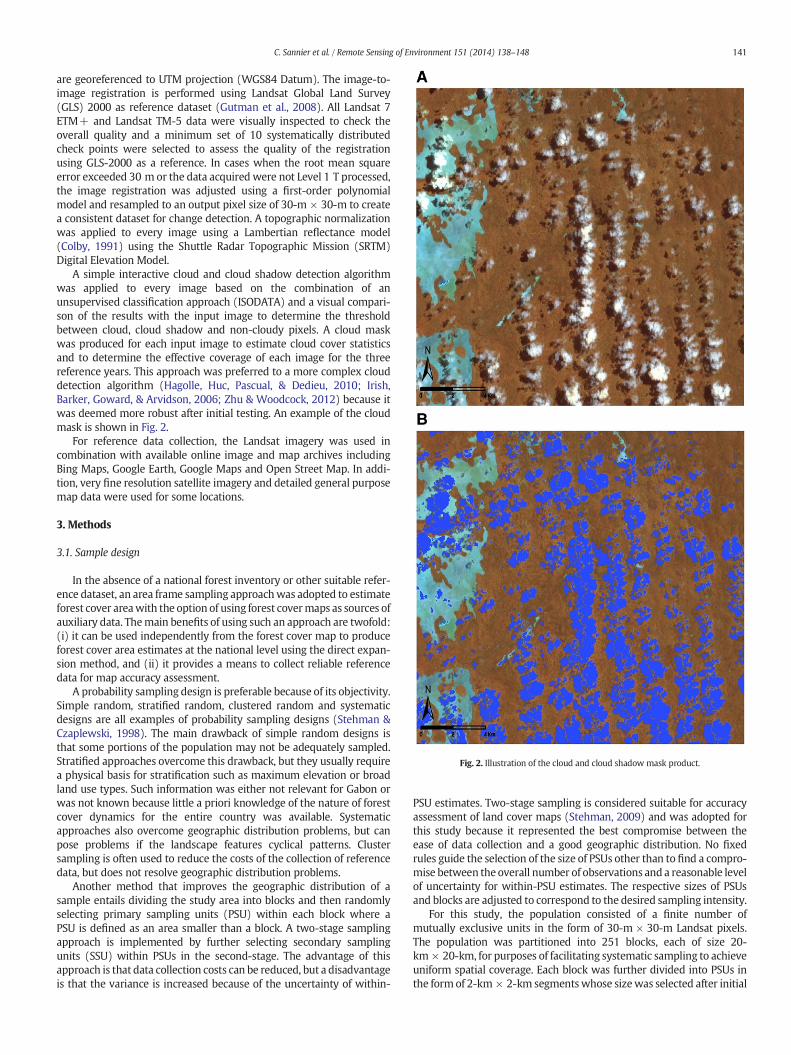
Fig. 2. Illustration of the cloud and cloud shadow mask product.

141C. Sannier et al. / Remote Sensing of Environment 151 (2014) 138–148

are georeferenced to UTM projection (WGS84 Datum). The image-to-image registration is performed using Landsat Global Land Survey(GLS) 2000 as reference dataset (Gutman et al., 2008). All Landsat 7ETM+ and Landsat TM-5 data were visually inspected to check theoverall quality and a minimum set of 10 systematically distributedcheck points were selected to assess the quality of the registrationusing GLS-2000 as a reference. In cases when the root mean squareerror exceeded 30 m or the data acquired were not Level 1 T processed,the image registration was adjusted using a first-order polynomialmodel and resampled to an output pixel size of 30-m × 30-m to createa consistent dataset for change detection. A topographic normalizationwas applied to every image using a Lambertian reflectance model(Colby, 1991) using the Shuttle Radar Topographic Mission (SRTM)Digital Elevation Model.

A simple interactive cloud and cloud shadow detection algorithmwas applied to every image based on the combination of anunsupervised classification approach (ISODATA) and a visual compari-son of the results with the input image to determine the thresholdbetween cloud, cloud shadow and non-cloudy pixels. A cloud maskwas produced for each input image to estimate cloud cover statisticsand to determine the effective coverage of each image for the threereference years. This approach was preferred to a more complex clouddetection algorithm (Hagolle, Huc, Pascual, & Dedieu, 2010; Irish,Barker, Goward, & Arvidson, 2006; Zhu & Woodcock, 2012) because itwas deemed more robust after initial testing. An example of the cloudmask is shown in Fig. 2.

For reference data collection, the Landsat imagery was used incombination with available online image and map archives includingBing Maps, Google Earth, Google Maps and Open Street Map. In addi-tion, very fine resolution satellite imagery and detailed general purposemap data were used for some locations.

3. Methods

3.1. Sample design

In the absence of a national forest inventory or other suitable refer-ence dataset, an area frame sampling approachwas adopted to estimateforest cover areawith the option of using forest covermaps as sources ofauxiliary data. Themain benefits of using such an approach are twofold:(i) it can be used independently from the forest cover map to produceforest cover area estimates at the national level using the direct expan-sion method, and (ii) it provides a means to collect reliable referencedata for map accuracy assessment.

A probability sampling design is preferable because of its objectivity.Simple random, stratified random, clustered random and systematicdesigns are all examples of probability sampling designs (Stehman &Czaplewski, 1998). The main drawback of simple random designs isthat some portions of the population may not be adequately sampled.Stratified approaches overcome this drawback, but they usually requirea physical basis for stratification such as maximum elevation or broadland use types. Such information was either not relevant for Gabon orwas not known because little a priori knowledge of the nature of forestcover dynamics for the entire country was available. Systematicapproaches also overcome geographic distribution problems, but canpose problems if the landscape features cyclical patterns. Clustersampling is often used to reduce the costs of the collection of referencedata, but does not resolve geographic distribution problems.

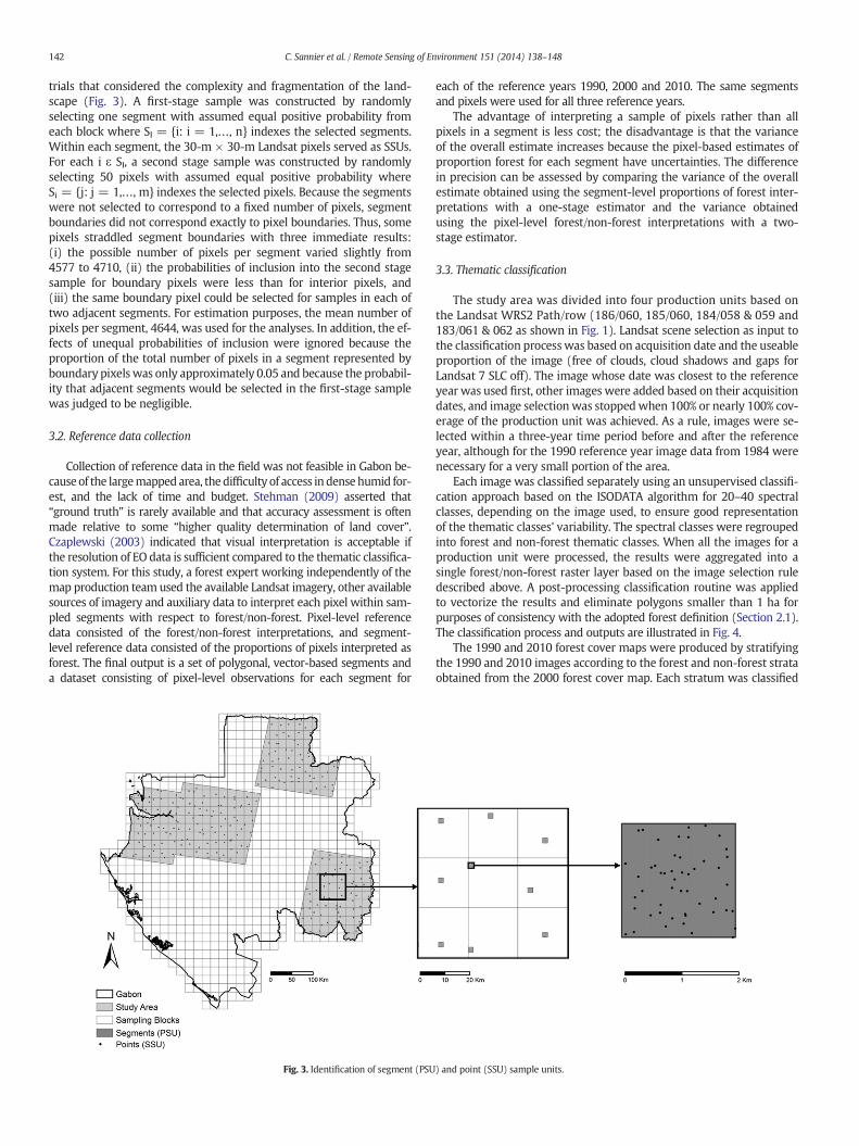
Another method that improves the geographic distribution of asample entails dividing the study area into blocks and then randomlyselecting primary sampling units (PSU) within each block where aPSU is defined as an area smaller than a block. A two-stage samplingapproach is implemented by further selecting secondary samplingunits (SSU) within PSUs in the second-stage. The advantage of thisapproach is that data collection costs can be reduced, but a disadvantageis that the variance is increased because of the uncertainty of within-

PSU estimates. Two-stage sampling is considered suitable for accuracyassessment of land cover maps (Stehman, 2009) and was adopted forthis study because it represented the best compromise between theease of data collection and a good geographic distribution. No fixedrules guide the selection of the size of PSUs other than to find a compro-mise between the overall number of observations and a reasonable levelof uncertainty for within-PSU estimates. The respective sizes of PSUsand blocks are adjusted to correspond to the desired sampling intensity.

For this study, the population consisted of a finite number ofmutually exclusive units in the form of 30-m × 30-m Landsat pixels.The population was partitioned into 251 blocks, each of size 20-km × 20-km, for purposes of facilitating systematic sampling to achieveuniform spatial coverage. Each block was further divided into PSUs inthe formof 2-km × 2-km segmentswhose sizewas selected after initial

142 C. Sannier et al. / Remote Sensing of Environment 151 (2014) 138–148

trials that considered the complexity and fragmentation of the land-scape (Fig. 3). A first-stage sample was constructed by randomlyselecting one segment with assumed equal positive probability fromeach block where SI = {i: i = 1,…, n} indexes the selected segments.Within each segment, the 30-m × 30-m Landsat pixels served as SSUs.For each i ε SI, a second stage sample was constructed by randomlyselecting 50 pixels with assumed equal positive probability whereSi = {j: j = 1,…, m} indexes the selected pixels. Because the segmentswere not selected to correspond to a fixed number of pixels, segmentboundaries did not correspond exactly to pixel boundaries. Thus, somepixels straddled segment boundaries with three immediate results:(i) the possible number of pixels per segment varied slightly from4577 to 4710, (ii) the probabilities of inclusion into the second stagesample for boundary pixels were less than for interior pixels, and(iii) the same boundary pixel could be selected for samples in each oftwo adjacent segments. For estimation purposes, the mean number ofpixels per segment, 4644, was used for the analyses. In addition, the ef-fects of unequal probabilities of inclusion were ignored because theproportion of the total number of pixels in a segment represented byboundary pixelswas only approximately 0.05 and because the probabil-ity that adjacent segments would be selected in the first-stage samplewas judged to be negligible.

3.2. Reference data collection

Collection of reference data in the field was not feasible in Gabon be-cause of the largemappedarea, thedifficulty of access in densehumid for-est, and the lack of time and budget. Stehman (2009) asserted that“ground truth” is rarely available and that accuracy assessment is oftenmade relative to some “higher quality determination of land cover”.Czaplewski (2003) indicated that visual interpretation is acceptable ifthe resolution of EO data is sufficient compared to the thematic classifica-tion system. For this study, a forest expert working independently of themap production team used the available Landsat imagery, other availablesources of imagery and auxiliary data to interpret each pixel within sam-pled segments with respect to forest/non-forest. Pixel-level referencedata consisted of the forest/non-forest interpretations, and segment-level reference data consisted of the proportions of pixels interpreted asforest. The final output is a set of polygonal, vector-based segments anda dataset consisting of pixel-level observations for each segment for

Fig. 3. Identification of segment (PSU

each of the reference years 1990, 2000 and 2010. The same segmentsand pixels were used for all three reference years.

The advantage of interpreting a sample of pixels rather than allpixels in a segment is less cost; the disadvantage is that the varianceof the overall estimate increases because the pixel-based estimates ofproportion forest for each segment have uncertainties. The differencein precision can be assessed by comparing the variance of the overallestimate obtained using the segment-level proportions of forest inter-pretations with a one-stage estimator and the variance obtainedusing the pixel-level forest/non-forest interpretations with a two-stage estimator.

3.3. Thematic classification

The study area was divided into four production units based onthe Landsat WRS2 Path/row (186/060, 185/060, 184/058 & 059 and183/061 & 062 as shown in Fig. 1). Landsat scene selection as input tothe classification process was based on acquisition date and the useableproportion of the image (free of clouds, cloud shadows and gaps forLandsat 7 SLC off). The image whose date was closest to the referenceyear was used first, other images were added based on their acquisitiondates, and image selection was stoppedwhen 100% or nearly 100% cov-erage of the production unit was achieved. As a rule, images were se-lected within a three-year time period before and after the referenceyear, although for the 1990 reference year image data from 1984 werenecessary for a very small portion of the area.

Each image was classified separately using an unsupervised classifi-cation approach based on the ISODATA algorithm for 20–40 spectralclasses, depending on the image used, to ensure good representationof the thematic classes' variability. The spectral classes were regroupedinto forest and non-forest thematic classes. When all the images for aproduction unit were processed, the results were aggregated into asingle forest/non-forest raster layer based on the image selection ruledescribed above. A post-processing classification routine was appliedto vectorize the results and eliminate polygons smaller than 1 ha forpurposes of consistency with the adopted forest definition (Section 2.1).The classification process and outputs are illustrated in Fig. 4.

The 1990 and 2010 forest cover maps were produced by stratifyingthe 1990 and 2010 images according to the forest and non-forest strataobtained from the 2000 forest cover map. Each stratum was classified

) and point (SSU) sample units.

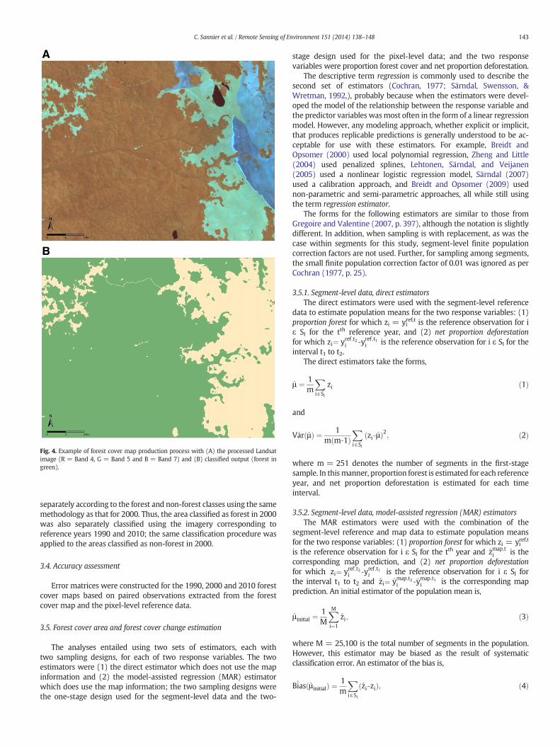
Fig. 4. Example of forest cover map production process with (A) the processed Landsatimage (R = Band 4, G = Band 5 and B = Band 7) and (B) classified output (forest ingreen).

143C. Sannier et al. / Remote Sensing of Environment 151 (2014) 138–148

separately according to the forest and non-forest classes using the samemethodology as that for 2000. Thus, the area classified as forest in 2000was also separately classified using the imagery corresponding toreference years 1990 and 2010; the same classification procedure wasapplied to the areas classified as non-forest in 2000.

3.4. Accuracy assessment

Error matrices were constructed for the 1990, 2000 and 2010 forestcover maps based on paired observations extracted from the forestcover map and the pixel-level reference data.

3.5. Forest cover area and forest cover change estimation

The analyses entailed using two sets of estimators, each withtwo sampling designs, for each of two response variables. The twoestimators were (1) the direct estimator which does not use the mapinformation and (2) the model-assisted regression (MAR) estimatorwhich does use the map information; the two sampling designs werethe one-stage design used for the segment-level data and the two-

stage design used for the pixel-level data; and the two responsevariables were proportion forest cover and net proportion deforestation.

The descriptive term regression is commonly used to describe thesecond set of estimators (Cochran, 1977; Särndal, Swensson, &Wretman, 1992,), probably because when the estimators were devel-oped the model of the relationship between the response variable andthe predictor variables wasmost often in the form of a linear regressionmodel. However, any modeling approach, whether explicit or implicit,that produces replicable predictions is generally understood to be ac-ceptable for use with these estimators. For example, Breidt andOpsomer (2000) used local polynomial regression, Zheng and Little(2004) used penalized splines, Lehtonen, Särndal, and Veijanen(2005) used a nonlinear logistic regression model, Särndal (2007)used a calibration approach, and Breidt and Opsomer (2009) usednon-parametric and semi-parametric approaches, all while still usingthe term regression estimator.

The forms for the following estimators are similar to those fromGregoire and Valentine (2007, p. 397), although the notation is slightlydifferent. In addition, when sampling is with replacement, as was thecase within segments for this study, segment-level finite populationcorrection factors are not used. Further, for sampling among segments,the small finite population correction factor of 0.01 was ignored as perCochran (1977, p. 25).

3.5.1. Segment-level data, direct estimatorsThe direct estimators were used with the segment-level reference

data to estimate population means for the two response variables: (1)proportion forest for which zi = yiref,t is the reference observation for iε SI for the tth reference year, and (2) net proportion deforestationfor which zi¼ yref ;t2i ‐yref ;t1i is the reference observation for i ε SI for theinterval t1 to t2.

The direct estimators take the forms,

μ ¼ 1m

Xiε SI

zi ð1Þ

and

Var μð Þ ¼ 1m m‐1ð Þ

Xi ε SI

zi‐μð Þ2; ð2Þ

where m = 251 denotes the number of segments in the first-stagesample. In thismanner, proportion forest is estimated for each referenceyear, and net proportion deforestation is estimated for each timeinterval.

3.5.2. Segment-level data, model-assisted regression (MAR) estimatorsThe MAR estimators were used with the combination of the

segment-level reference and map data to estimate population meansfor the two response variables: (1) proportion forest for which zi = yiref,t

is the reference observation for i ε SI for the tth year and zmap;ti is the

corresponding map prediction, and (2) net proportion deforestationfor which zi¼ yref ;t2i ‐yref ;t1i is the reference observation for i ε SI forthe interval t1 to t2 and zi¼ ymap;t2

i ‐ymap;t1i is the corresponding map

prediction. An initial estimator of the population mean is,

μ initial ¼1M

XM

i¼1

zi; ð3Þ

where M = 25,100 is the total number of segments in the population.However, this estimator may be biased as the result of systematicclassification error. An estimator of the bias is,

Bias μ initialð Þ ¼ 1m

Xi ε SI

zi‐zið Þ; ð4Þ

Table 1Summary of Landsat image data coverage for the selected study area corresponding toLandsat WRS2 P183R61, P183R62, P184R58, P184R59, P185R60 and P186R60.

Referenceyear

Imagedate

Area covered[km2]

Cumulativepercentage [%]

Number of Landsatimages processed

1990 1990 41729.6 40.7 51989 35442.5 75.3 71988 21045.1 95.8 151987 3158.6 98.9 81985 300.4 99.2 21984 163.0 99.4 4No data 639.9 100.0

2000 2000 94604.4 92.3 131999 1928.9 94.2 22001 5059.6 99.1 82002 791.1 99.9 92003 34.9 99.9 4No data 60.4 100.0

2010 2010 68551.2 66.9 72011 24475.0 90.8 102009 8105.2 98.7 82008 1036.2 99.7 32007 311.5 100.0 4No data 0.0 100.0

144 C. Sannier et al. / Remote Sensing of Environment 151 (2014) 138–148

wherem = 251 is the number of segments in thefirst-stage sample. TheMAR estimator (Särndal et al., 1992, Section 6.5) is defined as the differ-ence between the initial estimator and the bias estimator and isexpressed as,

μMAR¼ μ initial‐Bias μ initialð Þ

¼ 1M

XM

i¼1

zi‐1m

Xi ε SI

zi‐zið Þ:ð5Þ

An estimator of the variance of μMAR is

Var μMARð Þ ¼ 1m m‐1ð Þ

Xi ε SI

εi‐εð Þ2; ð6Þ

where εi¼ zi−zi and ε ¼ 1m ∑

i ε SIεi . In this manner, proportion forest

cover is estimated for each reference year, and net proportion defores-tation is estimated for each time interval.

3.5.3. Pixel-level data, direct estimatorsThe direct estimators were used with the pixel-level reference

data to estimate the population means for the two response variables:(1) proportion forest for which zij = yijref,t is the reference observationfor pixel j ε Si for the tth reference year, and (2) net proportion deforesta-tion forwhichzij¼ yref ;t2ij ‐yref ;t1ij is the reference observation for pixel j ε Sifor the interval t1 to t2. The direct estimators take the forms,

μ ¼ 1m� n

Xi ε SI

Xj ε Si

zij; ð7Þ

where n = 50 is the number of pixels sampled in each segment. Thus,the variance estimator is,

Var μð Þ ¼ s2bm

þ 1m�M

Xi ε SI

s2in; ð8Þ

where for i ε SI, Ni ≈ N = 4644 is the total number of pixels in eachsegment,

s2i ¼ 1n‐1

Xj ε Si

zij‐zi� �2

; ð9Þ

and

s2b ¼ 1m‐1

Xi ε SI

zi‐μð Þ2; ð10Þ

where the terms, s2bm and s2i

n , are estimates of variances. The forms ofthe estimators μ and Var μð Þ are simplified as the result of several sam-pling features and assumptions: (i) all segments were the same size,(ii) all segments were considered to contain the same number of pixels,and (iii) any effects of pixels straddling segment boundaries wereignored.

3.5.4. Pixel-level data, model-assisted regression (MAR) estimatorsTheMARestimators are usedwith the combination of the pixel-level

reference and map data to estimate the population means for tworesponse variables: (1) proportion forest for which zij = yijref,t is thereference observation for pixel j ε Si for the tth year with correspondingmap prediction, zij¼ ymap;t

ij , and (2) net proportion deforestation forwhich zij¼ yref ;t2ij ‐yref ;t1ij is the reference observation for j ε Si for the

interval t1 to t2 with corresponding map prediction, zij¼ ymap;t2ij ‐ymap;t1

ij .An initial estimator of the population mean is,

μ initial ¼1

MN

XM

i¼1

XN

j¼1

zij; ð11Þ

where M = 25,100 is the total number of segments in the populationand for all i ε SI, Ni ≈ N = 4644 is the number of pixels in eachsegment. An estimator of the bias resulting from systematic classifica-tion error is,

Bias μ initialð Þ ¼ 1m

Xi ε SI

zi‐zi� �

; ð12Þ

wherezi ¼ 1n ∑j ε Si

zij and zi ¼ 1n ∑j ε Si

zij. TheMAR estimator is defined as the

difference between the initial and bias estimators,

μMAR¼ μ initial‐Bias μ initialð Þ: ð13Þ

Under the assumption that for all i ε SI, Ni ≈ N = 4644, and thatsampling is with replacement within segments, an estimator of thevariance is,

Var μMARð Þ ¼ s2bm

þ 1m�M

Xi ε SI

s2in; ð14Þ

where

s2i ¼ 1n‐1

Xj ε Si

εij‐εi� �2

;

s2b ¼ 1m‐1

Xj ε Si

εi‐εð Þ2;

εij¼ zij‐zij;

εi ¼1n

Xj ε Si

εij;

and

ε ¼ 1m

Xi ε SI

εi:

Fig. 5. Forest cover change maps for (A) 1990–2000 and (B) 2000–2010.

145C. Sannier et al. / Remote Sensing of Environment 151 (2014) 138–148

4. Results and discussion

4.1. Image acquisition

Overall, 123 Landsat images were required to obtain sufficient cloudfree coverage for reference years 1990, 2000, and 2010 due to the largelevel of cloud cover. An average of six, but as many as nine Landsatimages were required to cover the area represented by a single scene.The average cloud cover was 42% for the images used in map produc-tion, but reached 55% for WRS2 186/061.

Complete coverage for each reference year was not possible(Table 1). For reference year 2000, cloud-free imagery was obtained

for 93% of the study area; however, for reference year 2010 cloud-freeimagery was obtained for only 67% of the study area, and for referenceyear 1990, the percentage was only 41%. However, 95% of the areacould be covered using imagery within two years of the reference year1990, and nearly 99% within one year of both reference years 2000and 2010. Overall, less than 1% of the study area could not be coveredfor any of the reference years with 1990 being the most difficult.These results demonstrate that optical imagery and the Landsat archivein particular are suitable for wall-to-wall forest cover mapping in acloud-prone country such as Gabon. They also reinforce the benefits ofacquiring and maintaining a systematic, time series archive of observa-tions of the Earth's surface. Of particular note, therewas no indication in

Table 2Errormatrices for the 1990, 2000 and2010 forest covermaps based on SSUs (n = 12550).

Reference

Forest Non-forest Total User'saccuracy

1990 Forest 10,609 124 10,733 0.9884Classification Non-forest 161 1656 1817 0.9114Total 10,770 1780 12,550Producer's accuracy 0.9851 0.9303 Overall

accuracy0.9773

2000 Forest 10,565 117 10,682 0.9890Classification Non-forest 173 1695 1868 0.9074Total 10,738 1812 12,550Producer's accuracy 0.9839 0.9354 Overall

accuracy0.9769

2010 Forest 10,575 103 10,678 0.9904Classification Non-forest 170 1702 1872 0.9092Total 10,745 1805 12,550Producer's accuracy 0.9842 0.9429 Overall

accuracy0.9782

(a)

(b)

y = xR² = 0,9767

0,00

0,10

0,20

0,30

0,40

0,50

0,60

0,70

0,80

0,90

1,00

0,00 0,10 0,20 0,30 0,40 0,50 0,60 0,70 0,80 0,90 1,00

Pro

port

ion

(Seg

men

t cla

ss)

Proportion (Segment Ref)

y = xR² = 0,9793

0,30

0,40

0,50

0,60

0,70

0,80

0,90

1,00

Pro

port

ion

(Seg

men

t cla

ss)

146 C. Sannier et al. / Remote Sensing of Environment 151 (2014) 138–148

the 1980s and 1990s that Landsat imagery acquired in those yearswould be so indispensable for forest covermapping at later dates.More-over, one Landsat satellite is not sufficient to provide annual cloud-freecoverage for a country such as Gabon. Although the lack of satellite datafor estimating long-term rates of deforestation may not be seriouslydetrimental, it will be problematic if forest cover is to be monitoredon an annual basis for management and legal enforcement purposes.Thus, the launch of Landsat 8 and especially Sentinel 2a and b are partic-ularly welcome for these applications. Finally, studies such as this onethat requires more than 40 Landsat images for each reference yearwould not be possible without Landsat's free and open data accesspolicy.

0,00

0,10

0,20

0,00 0,10 0,20 0,30 0,40 0,50 0,60 0,70 0,80 0,90 1,00

Proportion (Segment Ref)

(c)

y = xR² = 0,9805

0,00

0,10

0,20

0,30

0,40

0,50

0,60

0,70

0,80

0,90

1,00

0,00 0,10 0,20 0,30 0,40 0,50 0,60 0,70 0,80 0,90 1,00

Pro

port

ion

(Seg

men

t cla

ss)

Proportion (Segment Ref)

Fig. 6. Comparison ofmap class (class) and reference (ref) observation forest proportion atthe segment level for the (a) 1990, (b) 2000, and (c) 2010 forest/non-forest maps.

4.2. Accuracy assessment

Fig. 5 illustrates the forest cover maps and indicates that changes inthe levels of net deforestation measured were extremely small. Con-struction of error matrices using all pixels contained within segmentswould have led to the inclusion of a large number of non-independentspatially contiguous observations. Therefore, error matrices wereconstructed using only the pixels selected for the second-stage sample.The results are detailed in Table 2 and are very consistent across thethree forest cover maps. Overall accuracies were all close to 98%, andneither producer nor user accuracies were less than 90%. Furthermore,there were no obvious imbalances in the error distributions, meaningthat omission errors were nearly equal to commission errors with theresult that bias estimates associated with the initial estimates weresmall.

The reference data were acquired independently from map produc-tion by visual interpretation of the available satellite imagery by aforestry expert with extensive experience. Thus, the reference datacan suffer from errors, although such errors are less likely than for themap production process. The reason is that interpreters focused onsmaller areas andwere able to use data from all available sources. Errorsor disagreements with the map are most likely attributable to thefollowing causes:

• Geometry of features detected: the reference data are likely to bemore precise, particularly when very fine resolution imagery wasavailable;

• Differences in image acquisition dates: the imagery used to producethe reference data was selected independently from the imageryused for map production with the result that the two image datesmay differ by a small number of years;

• Errors in the map or reference data.

However, considering the high level of agreement between themapand reference data, errors may be assumed to be few and production ofreference data may be assumed to be possible, particularly when thereis a sharp spectral difference between forest, which is almost entirelyevergreen in Gabon, and non-forest.

Table 3Estimates of proportion forest cover and net proportion deforestation from points;estimates in bold indicate estimates that are not significantly different from 0 (SE =Standard Error).

Forest cover Forest cover change

1990 2000 2010 1990–2000 2000–2010 1990–2010

Direct mean 0.8552 0.8512 0.8508 −0.0041 −0.0003 −0.0044Direct SE 0.0186 0.0187 0.0188 0.0020 0.0013 0.0030Map estimate 0.8633 0.8616 0.8613 −0.0017 −0.0003 −0.0020Bias estimate 0.0029 0.0045 0.0053 0.0015 0.0009 0.0024MAR estimate 0.8604 0.8571 0.8560 −0.0033 −0.0011 −0.0044MAR SE 0.0032 0.0031 0.0029 0.0012 0.0012 0.0016

147C. Sannier et al. / Remote Sensing of Environment 151 (2014) 138–148

These results were confirmed at the segment-level as shown inFig. 6. For the forest/non-forest maps for all three reference years, theestimates of forest proportions based on the reference datawere similarto the proportions for the segments. However, the maps for each refer-ence year had a few segments for which the differences were large,although systematic errors were not evident. A simple linear regressionmodel fit to the reference observations as the dependent variable andthe corresponding predictions as the independent variable (Fig. 6)produced R2 = 0.98, and estimates of the intercept and slope wereclose to 1 and 0, respectively, thus confirming the results obtainedfrom the error matrices.

4.3. Forest cover and forest cover change estimates

When comparing the direct and the MAR estimates of proportionforest for the pixel-level dataset (Table 3), two results were notewor-thy: (i) the large accuracies of the maps were indicated by the similari-ties between the direct and the map-based estimates and by the smallbias estimates, and (ii) the smaller standard errors (SE) for the MARestimates relative to the direct estimates could be attributed to therelevance of the auxiliary information on which the maps are based.

When comparing the direct and MAR estimates of net proportiondeforestation, five results were noteworthy: (i) the large accuracies ofthe maps were indicated by the similarities between the direct andthemap-based estimates and by the small bias estimates, (ii) the adjust-ments for estimated biases producedMAR estimates that were closer tothe direct estimates than the map-based estimates, (iii) the relativeequality of the direct estimates of SEs and the MAR estimates of SEswas attributed to the fact that the SEs were already very small, i.e.,very little improvement was even possible, (iv) the very small SEs forestimates of net proportion deforestation relative to the SEs forestimates of proportion forest were attributed to the beneficial effectsof using the same reference pixels for all three classifications; this resultis similar to the benefit obtained using a paired t-test as opposed to thestandard t-test, and (v) at the approximate α = 0.05 level of signifi-cance, none of the 2000–2010 estimates (direct and MAR) were signif-icantly different from 0. The latter result was not surprising consideringthe even smaller estimate of net deforestation compared to that of1990–2000. The fact that the 1990–2010 direct expansion estimate(−0.44%) was not significantly different from 0 was more surprising.

Table 4Estimates of proportion forest cover and net proportion deforestation from segments;estimates in bold indicates estimates that are not significantly different from 0 (SE =Standard Error).

Forest cover Forest cover change

1990 2000 2010 1990–2000 2000–2010 1990–2010

Direct mean 0.8568 0.8534 0.8532 −0.0034 −0.0002 −0.0036Direct SE 0.0185 0.0186 0.0186 0.0021 0.0009 0.0027Map estimate 0.8633 0.8616 0.8613 −0.0017 −0.0003 −0.0020Bias estimate 0.0027 0.0042 0.0049 0.0015 0.0007 0.0023MAR estimate 0.8606 0.8574 0.8564 −0.0032 −0.0010 −0.0043MAR SE 0.0028 0.0026 0.0025 0.0009 0.0008 0.0012

However, this was in contrast to the MAR estimate (−0.44%) forwhich the SE was much smaller (0.30% versus 0.16%).

These results were further confirmed by the segment-level esti-mates (Table 4) which were very similar to the pixel-level estimatesfor the proportion forest cover and net proportion deforestation,although SEs were even smaller. Both 2000–2010 estimates were notsignificantly different from 0, and all other estimates were significantlydifferent from 0 which is consistent with the level of net deforestationobserved.

Although the SEs in Table 3 did not so indicate, the among-segmentsportions of the variance estimates dominated the within-segmentsportions of the variance estimates. A minor contribution to this resultmay be that among-segments variance estimates were slightly inflatedas a result of using a systematic rather than a simple random samplingdesign to select the first-stage segments (Särndal et al., 1992). Thesmallness of the within-segments variance relative to the among-segments variance should not be surprising given the large accuraciesof the classifications and the relatively large within-segments referencesample size, n = 50. For future considerations, even smaller overall SEsfor both direct and MAR estimates could perhaps be obtained for thesame number of pixels by selecting more segments but with fewerpixels within each segment. However, for this study, the objective ofsmall standard errors was certainly achieved, so in this sense the designwas appropriate. In addition, there was little, if any, prior knowledge ofthe relative sizes of the among- and within-segments variances.

5. Conclusions

The use of the model-assisted regression estimator reduced thevariances of the proportion forest cover estimates by a factor of approx-imately 50, meaning that to obtain equivalent results using only asampling approach, the sample size would have to be increased by thesame factor. In addition, there were differences between the map-based and MAR estimates of net deforestation despite the very largeaccuracies for the forest cover maps. Thus, even though large mappingaccuracies can be achieved, map-based estimates without adjustmentfor estimated biases should be used cautiously. Nevertheless, all resultsexhibited the same overall trend: direct expansion estimates could beproduced rapidly and used to report reliable estimates of net proportiondeforestation, while wall-to-wall maps could be used to refine thoseestimates and to support more detailed investigations.

In addition, pixel-level estimates exhibited slightly greater SEs thansegment-level estimates, but the differences were small, particularlywhen the forest cover maps were used as auxiliary information. There-fore, a two-stage sampling approach was justified for collecting reliableforest cover reference data to estimate proportion forest cover and netproportion deforestation.

The results confirmed the generally small level of net deforestationexpected in Gabon. Further, the estimates of net proportion deforesta-tion were significantly different from 0 for all estimates for the period1990–2000, whereas they were all not significantly different fromzero for the period 2000–2010. The smaller rate of net proportion defor-estation estimated for the latter 10 years could be explained by the cre-ation of national parks and the implementation of forest concessionmanagement plans from 2000 onward, although the link betweenGabonese environmental policies and the estimated reduced level offorest loss should be further explored.

However, the coefficients of variation for net proportion deforesta-tion estimates were large compared to the coefficients for the propor-tion forest cover estimates. This result is likely attributable to aweaker relationship between the reference and map data, probably forthe reasons outlined in Section 4.2 (mismatch in geometry, temporaldifferences, and actual interpretation errors). The estimated level ofnet proportion deforestation was small, approximately 0.04% perannum for the 1990–2000 period.

148 C. Sannier et al. / Remote Sensing of Environment 151 (2014) 138–148

The nature of forest dynamics in Gabon makes finding a sound basisfor stratification difficult because the majority of gross deforestation islinked to forest exploitation and can occur at any time in forest conces-sions which are scattered over the entire country. A more thorough un-derstanding of deforestation drivers and causes is required but wasbeyond the scope of this study.

Finally, the approach developed for 38% of Gabon was subsequentlyapplied to the entire country for 1990 and 2000; the analyses for 2010are still progress. Initial results confirm those obtained for the 38%with a similar estimate of the net proportion deforestation rate. The95% confidence interval width represents approximately 0.25% of theproportion forest cover estimates and represents 88.4% of the overallarea of the country, making forest cover in Gabon even greater thanhad been previously thought.

These results demonstrate that despite Gabon's heavy cloud cover,imagery for the entire study area could be acquired. However, thelarge amount of cloud cover meant that on average six Landsat imageswere required to cover the area of a single Landsat scene. Nevertheless,the methodology was sufficiently robust and simple to implement thatit can be readily implemented in Gabon and other similar tropicalcountries.

Acknowledgments

The production of forest cover and forest cover change maps wasfunded under the European Space Agency (ESA) Global Monitoring forthe Environment and Security Service Element on Forest MonitoringREDD extension project (GSE FMREDD). Methodological developmentsrelated to forest cover area and forest cover change area estimates werefunded under the EU FP7 GMES REDDAF project. Both projects were co-ordinated by GAF AG. The authors thank Professor Timothy G. Gregoire,Yale University, for consultations on and references for the model-assisted, regression estimator.

References

Achard, F., DeFries, R., Eva, H., Hansen, M., Mayaux, P., & Stibig, H. -J. (2007). Pan-tropicalmonitoring of deforestation. Environmental Research Letters, 2, 11pp.

Achard, F., Eva, H. D., Mayaux, P., Gallego, J., Richards, T., & Malingreau, J. -P. (2002).Determination of deforestation rates of the world' s humid tropical forests. Science,297, 999–1002.

Allen, J.D. (1990). A look at the remote sensing applications program of the NationalAgricultural Statistics Service. Journal of Official Statistics, 6, 393–409.

Breidt, F. J., & Opsomer, J.D. (2000). Local polynomial regression estimators in surveysampling. The Annals of Statistics, 28(4), 1026–1053.

Breidt, F. J., & Opsomer, J.D. (2009). Nonparametric and semiparametric estimation incomplex surveys. In D. Pfeffermann, & C. R. Rao (Eds.), Handbook of statistics — samplesurveys: inference and analysis, Vol. 29B. (pp. 103–120)The Netherlands: North-Holland.

Carfagna, E., & Gallego, J. (2005). Using remote sensing for agricultural statistics.International Statistical Review, 73, 389–404.

Central Intelligence Agency (CIA) (2012). The World Factbook. https://www.cia.gov/library/publications/the-world-factbook/index.html (last accessed 27/03/2013).

Cochran, W. G. (1977). Sampling techniques (3rd ed.), New York: Wiley (428 pp.).Colby, J.D. (1991). Topographic normalization in rugged terrain. Photogrammetric

Engineering & Remote Sensing, 57, 531–537.Congalton, R. G. (1991). A review of assessing the accuracy of classifications of remotely

sensed data. Remote Sensing of Environment, 37, 35–46.Czaplewski, R. L. (2003). Chapter 5: accuracy assessment of maps of forest condition: sta-

tistical design andmethodological considerations, pp. 115–140. InMichael A.Wulder,& Steven E. Franklin (Eds.), Remote sensing of forest environments: concepts and casestudies. Boston: Kluwer Academic Publishers (515 pp.).

de Wasseige, C., de Marcken, P., Bayol, N., Hiol Hiol, F., Ph, Mayaux, Desclée, B., et al.(2012). Les forêts du bassin du Congo — Etat des Forêts 2010, Office des publicationsde l'Union Européenne, Luxembourg978-92-79-22717-2 (276 pp.).

Deppe, F. (1998). Forest area estimation using sample surveys and Landsat MSS and TMdata. Photogrammetric Engineering and Remote Sensing, 64, 285–292.

Duveiller, G., Defourny, P., Desclée, B., & Mayaux, P. (2008). Deforestation in CentralAfrica: estimates at regional, national and landscape levels by advanced processingof systematically-distributed Landsat extracts. Remote Sensing of Environment, 112,1969–1981.

Ernst, C., Mayaux, P., Verhegghen, A., Bodart, C., Christophe, M., & Defourny, P. (2013). Na-tional forest cover change in Congo Basin: deforestation, reforestation, degradationand regeneration for the years 1990, 2000 and 2005. Global Change Biology, 19,1173–1187. http://dx.doi.org/10.1111/gcb.12092.

Gallego, F. J. (2004). Remote sensing and land cover area estimation. International Journalof Remote Sensing, 25, 3019–3047.

GOFC-GOLD (2011). A sourcebook of methods and procedures for monitoring and reportinganthropogenic greenhouse gas emissions and removals caused by deforestation, gainsand losses of carbon stocks in forest raining forests, and forestation. GOFC-GOLD Reportversion COP17-1 (203 pp. Available ar: http://www.gofcgold.wur.nl/redd/index.php)

Gregoire, T. G., & Valentine, H. T. (2007). Sampling techniques for natural and environmen-tal resources. Boca Raton: Chapman & Hall/CRC (496 pp.).

Gullison, R. E., Frumhoff, P. C., Canadell, J. G., Field, C. B., Daniel, C., Hayhoe, K., et al. (2007).Tropical forests and climate policy. Science, 316, 985–986.

Gutman, G., Byrnes, R., Masek, J., Covington, S., Justice, C., Franks, S., et al. (2008). Towardsmonitoring land-cover and land-use changes at a global scale: the global land survey2005. Photogrammetric Engineering & Remote Sensing, 74, 6–10.

Hagolle, O., Huc, M., Pascual, D.V., & Dedieu, G. (2010). A multi-temporal method forcloud detection, applied to FORMOSAT-2, VENμS, LANDSAT and SENTINEL-2 images.Remote Sensing of Environment, 114, 1747–1755.

Hansen,M. C., Roy, D. P., Lindquist, E., Adusei, B., Justice, O. C., & Alstatt, A. (2008). A meth-od for integrating MODIS and Landsat data for systematic monitoring of forest coverchange in the Congo Basin. Remote Sensing of Environment, 112, 2495–2513.

IPCC (2006). IPCC guidelines for national greenhouse gas inventories, volume 4 (agricul-ture, forestry and other land use), National Greenhouse Gas Inventories program. InH. S. Eggleston, L. Buendia, K. Miwa, T. Ngara, & K. Tanabe (Eds.), Hayama: IGES(Available at: http://www.ipcc-nggip.iges.or.jp/public/2006gl/vol4.html)

Irish, R. R., Barker, J. L., Goward, S. N., &Arvidson, T. (2006). Characterization of the Landsat-7ETM automated cloud-cover assessment (ACCA) algorithm. PhotogrammetricEngineering and Remote Sensing, 72, 1179–1188.

Justice, C., Wilkie, D., Zhang, Q., Brunner, J., & Donoghue, C. (2001). Central African forests,carbon and climate change. Climate Research, 17, 229–246.

Lehtonen, R., Särndal, C. -E., & Veijanen, A. (2005). Does the model matter? Comparingmodel-assisted and model-dependent estimators of class frequencies for domains.Statistics in Transition, 7(3), 649–673.

Loveland, T. R., & Dwyer, J. L. (2012). Landsat: building a strong future. Remote Sensing ofEnvironment, 122, 22–29.

McRoberts, R. E. (2011). Satellite image-based maps: scientific inference or prettypictures? Remote Sensing of Environment, 115, 715–724.

McRoberts, R. E. (2014). Post-classification approaches to estimating change in forest areausing remotely sensed auxiliary data. Remote Sensing of Environment, 151, 149–156.

McRoberts, R. E., & Walters, B. F. (2012). Statistical inference for remote sensing-basedestimates of net deforestation. Remote Sensing of Environment, 124, 394–401.

Särndal, C. -E. (2007). The calibration approach in survey theory and practice. SurveyMethodology, 33(2), 99–119.

Särndal, C. -E., Swensson, B., & Wretman, J. (1992). Model assisted survey sampling. NewYork: Springer-Verlag, Inc (694 pp.).

Stehman, S. V. (1997). Selecting and interpreting measures of thematic classificationaccuracy. Remote Sensing of Environment, 62, 77–89.

Stehman, S. V. (2009). Sampling designs for accuracy assessment of land cover.International Journal of Remote Sensing, 30, 5243–5272.

Stehman, S. V., & Czaplewski, R. L. (1998). Design and analysis for thematic mapaccuracy assessment: fundamental principles. Remote Sensing of Environment, 64,331–334.

Taylor, J., Sannier, C., Delincé, J., & Gallego, F. J. (1997). Regional crop inventories in Europeassisted by remote sensing: 1988–1993. Synthesis report. Luxembourg: Office for Publi-cations of the EC.

UNFCCC (2006). Decision 16/CMP.1. http://unfccc.int/resource/docs/2005/cmp1/eng/08a03.pdf#page=3 (accessed on 5 November 2012).

Vibrans, A.C.,McRoberts, R. E.,Moser, P., &Nicoletti, A. L. (2013). Using satellite image-basedmaps and ground inventory data to estimate the area of the remainingAtlantic forest inthe Brazilian state of Santa Catarina. Remote Sensing of Environment, 130, 87–95.

Wulder, M.A., Masek, J. G., Cohen, W. B., Loveland, T. R., & Woodcock, C. E. (2012). Open-ing the archive: how free data has enabled the science and monitoring promise ofLandsat. Remote Sensing of Environment, 122, 2–10.

Zheng, H., & Little, R. J. A. (2004). Penalized spline nonparametric mixed models for infer-ence about a finite populationmean from two-stage samples. SurveyMethodology, 30,209–218.

Zhu, Z., & Woodcock, C. E. (2012). Object-based cloud and cloud shadow detection inLandsat imagery. Remote Sensing of Environment, 118, 83–94.

Zhu, Z., Woodcock, C. E., & Olofsson, P. (2012). Continuous monitoring of forestdisturbance using all available Landsat imagery. Remote Sensing of Environment, 122,75–91.