Embed Size (px)
Citation preview

GIS Ostrava 2013 - Geoinformatics for City Transformation January 21 – 23, 2013, Ostrava
REMOTE SENSING AND FIELD STUDIES TO EVALUATE THE PERFORMANCE OF GROYNES IN PROTECTING
AN ERODING STRETCH OF THE COASTAL CITY OF CHENNAI
Sanjeevi, SHANMUGAM1, Jayaprakash, NAYAK2
1, 2Department of Geology, Anna University, Chennai-600025, India
[email protected], [email protected]
Abstract
The city of Chennai, on the Coromandel Coast in south east India, has been facing the problem of severe
coastal erosion due to improper coastal engineering practices. The landward displacement of the shoreline
caused by the forces of waves and currents has been a perennial problem for the Chennai coast since the
last 100 years. In 2004, groynes were constructed along the north Chennai coast and the lost shoreline and
the beaches are now being regained. This study is concerned with remote sensing, GIS and field based
studies to evaluate the performance of these groynes along the north Chennai coast and quantify the rate of
accretion. Digitally processed multi-temporal (1972-2011) satellite images were interpreted and the
shorelines for 7 different years were digitised in a GIS environment. The digitised shorelines, imported into
the USGS developed Digital Shoreline Analysis System (DSAS) were analysed and final maps were
generated depicting erosion in pre-2004 and accretion in post-2004 periods.
These maps show that the shoreline has eroded about 220 meters in the last 32 years up to 2004, while it is
accreting at a rate of about 8 m/yr from 2004 up to 2011. Finally a shoreline change prediction model was
prepared in the DSAS environment. The positions of the future shorelines were determined using a
component of DSAS called LRR and the position of predicted shorelines was obtained. This study has
shown that due to the construction of groynes, erosion has reduced and deposition is in progress to regain
the lost beaches in Chennai City, thus indicating that the groynes are performing well.
Keywords: Chennai city, coastal protection, groynes, multi-date satellite images, GIS, DSAS
INTRODUCTION
Construction of coastal structures and dredging activities for the development of ports interfere in the coastal
processes of a region (Kudale, 2010). Sea level rise has also been an important factor responsible for
coastal erosion. Wang (1998) mentions that the increasing sea-level along China’s coast in the recent past,
has enhanced erosion by waves breaking on the upper beaches. The author observes that river-channel
slopes have been reduced and fluvial sediment discharges to the ocean have decreased, thus resulting in
increased coastal erosion. He finally concludes that all such effects are the result of human impact. Xia et al
(1993) noted that 70% of the sandy coasts in China are prone to erosion, thus threatening villages, roads,
factories, coast-protection forests and tourism. The speed of erosion ranges between 1 and 2 m/ yr in
general.
The city of Chennai (erstwhile Madras), which adorns the Coromandel coast in south east India, boasts of
the marina which is the world’s second longest beach. This coastal city, however, has been facing certain
problems. In its report, the Integrated Coastal and Marine Area Management Project Directorate, India
mentions that “it is well known that the shoreline along Chennai coast is subjected to oscillations due to
natural and man made activities. After construction of Chennai port, the coast north of the port is eroded and
350 hectares land is lost into sea. The state government resorted to short term measures for protecting the
coastal stretch with sea wall and the erosion problem shifted to further north” (ICMAM. 2006). Since there
has been severe erosion since the past 100 years, preventive measures such as construction of ten groynes
in the stretch between Royapuram and Ramakrishna Nagar along the Ennore expressway by the National
Highways Authority of India and the Tamilnadu Road Development Company have been implemented. Such
measures have helped reclaim the shoreline by a few metres. The department hopes to reclaim shoreline up
to 130 metres in two decades (The Hindu, 2012). After the construction of groynes in this area, it is

GIS Ostrava 2013 - Geoinformatics for City Transformation January 21 – 23, 2013, Ostrava
necessary that we study accretion, if any, due to the construction. It is also necessary that we estimate the
rate of accretion and evaluate the performance of the gryones. Accordingly, the objectives of this paper are:
(i) to use multi-temporal satellite image data and quantify erosion along the shoreline before the construction
of groynes, and accretion along the shoreline after the construction of groynes (ii) to use a prediction model
and predict the position of shoreline in the next decade.
Fig 1. Map of India and study area (left) and the satellite image of Chennai city (right) showing the gryones.
Study area
Chennai city lies on a flat coastal plain on the south east coast of India, known as the Coromandel Coast.
The climate is tropical wet and dry, and for most of the year, the weather is hot and humid, with temperatures
ranging from a maximum of 42°C in May to a minimum of 18°C in January. Most of the rainfall is received
from the northeast monsoon winds, from mid-October to mid-December. Cyclones in the Bay of Bengal also
hit the coast. The annual rainfall is about 1250 mm, and the spring tides are up to 1.2 m. Historically, the
Chennai port was responsible for the shoreline changes in the region, where the area south of the port has
accreted significantly, resulting in the formation of the Marina Beach, whereas the coast in the northern
region has undergone severe erosion. Ever since the harbour was constructed, the coast north of the
harbour has been experiencing erosion at the rate of about 8 m annually. The shoreline has recessed by
about 1,000 m with respect to the original shoreline in 1876. It is estimated that 500 m of beach has been
lost between 1876 and 1975 and another 200 m between 1978 and 1995. About 350 ha land in the coast
north of the port is lost into sea. On the other hand, the area south of the port is increasing 40 sq m every
year due to the progradation (EARSeL, 2002).
The study area (Figure 1) is between Chennai and Ennore ports where the groynes have been constructed.
The Ennore- Manali road forms the main communication link. The ten groynes are located each at an
interval of about 500-1000 meters over 6 kilometres. Sea wall has also been constructed to reduce erosion.
The groynes vary in length from 165-300 m and their height is 4m above MSL. These gryones have been
performing well by enhancing accretion. Analysis of historical sea level data for the Chennai coast indicates
that since 2004, co-incidentally, there is a trend of decrease in sea level. This could, in turn, result in
reduction in the incidence of erosion, or perhaps accelerate accretion along the Chennai coast.
METHODOLOGY
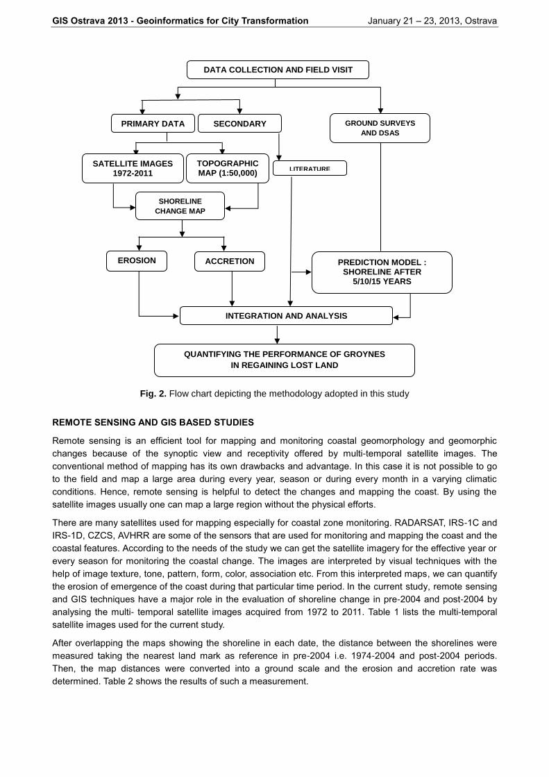
The methodology adopted for this study is shown in Figure 2. The main components of the methodology
include : (i) Remote sensing, (ii) GIS analysis (iii) Preparation of shoreline change model and predicting the
future shorelines. The individual components of the methodology listed in Figure 2 have been described in
detail in the following sections.
INDIA
Bay of
Bengal
GIS Ostrava 2013 - Geoinformatics for City Transformation January 21 – 23, 2013, Ostrava
Fig. 2. Flow chart depicting the methodology adopted in this study
REMOTE SENSING AND GIS BASED STUDIES
Remote sensing is an efficient tool for mapping and monitoring coastal geomorphology and geomorphic
changes because of the synoptic view and receptivity offered by multi-temporal satellite images. The
conventional method of mapping has its own drawbacks and advantage. In this case it is not possible to go
to the field and map a large area during every year, season or during every month in a varying climatic
conditions. Hence, remote sensing is helpful to detect the changes and mapping the coast. By using the
satellite images usually one can map a large region without the physical efforts.
There are many satellites used for mapping especially for coastal zone monitoring. RADARSAT, IRS-1C and
IRS-1D, CZCS, AVHRR are some of the sensors that are used for monitoring and mapping the coast and the
coastal features. According to the needs of the study we can get the satellite imagery for the effective year or
every season for monitoring the coastal change. The images are interpreted by visual techniques with the
help of image texture, tone, pattern, form, color, association etc. From this interpreted maps, we can quantify
the erosion of emergence of the coast during that particular time period. In the current study, remote sensing
and GIS techniques have a major role in the evaluation of shoreline change in pre-2004 and post-2004 by
analysing the multi- temporal satellite images acquired from 1972 to 2011. Table 1 lists the multi-temporal
satellite images used for the current study.
After overlapping the maps showing the shoreline in each date, the distance between the shorelines were
measured taking the nearest land mark as reference in pre-2004 i.e. 1974-2004 and post-2004 periods.
Then, the map distances were converted into a ground scale and the erosion and accretion rate was
determined. Table 2 shows the results of such a measurement.
INTEGRATION AND ANALYSIS
SHORELINE
CHANGE MAP
EROSION
BEFORE
ACCRETION
AFTER 2004
PREDICTION MODEL : SHORELINE AFTER
5/10/15 YEARS
QUANTIFYING THE PERFORMANCE OF GROYNES
IN REGAINING LOST LAND
GROUND SURVEYS
AND DSAS
DATA COLLECTION AND FIELD VISIT
PRIMARY DATA SECONDARY
DATA
SATELLITE IMAGES 1972-2011
TOPOGRAPHIC MAP (1:50,000)
LITERATURE

GIS Ostrava 2013 - Geoinformatics for City Transformation January 21 – 23, 2013, Ostrava
Table 1. Multi-temporal satellite images used in the study
Sl. No DATE OF IMAGE SENSOR RESOLUTION (m)
1 16/09/1972 LANDSAT MSS 80
2 25/08/1991 LANDSAT TM 30
3 28/10/2000 LANDSAT ETM 15
4 29/12/2004 IKONOS 1.0
5 06/04/2009 LANDSAT TM 30
6 02/09/2011 LANDSAT ETM 15
Fig. 3. Satellite images (1972 to 2011) showing the positing of shorelines
Table 2. Erosion and accretion along the land marks in pre-2004 and post-2004
LANDMARK
(Also see Fig.1)
1972-2004
Coastline change mtrs(≈)
2004-2011
Coastline change in mtrs(≈)
Erosion
(In mtrs)
Rate of erosion
(m/yr)
Accretion
(In mtrs)
Rate of accretion
(m/yr)
LANDMARK-1 (GROYNE-10) -170 5.3 +22 3.1
LANDMARK-2 (GROYNE-5) -225 7.03 +69 9.8
LANDMARK-3 (GROYNE-1) -316 9.1 +55 7.8
Bay
of
Be
nga
l

GIS Ostrava 2013 - Geoinformatics for City Transformation January 21 – 23, 2013, Ostrava
The results obtained by the shoreline change analysis using remote sensing and GIS based studies clearly
indicates that there was severe erosion at a rate of approximately 9.1 m/yr near to groyne No – 1 (Landmark-
3) upto 2004. However, after the construction of groynes in 2004 accretion took place at a rate of about
7.8m/yr. There was a low rate of erosion (5.3 m/yr) near to Groyne No – 10 (landmark-1) upto 2004 and
accretion started at a rate of about 3.1m/yr after 2004. Again in south of groyne No - 5 the erosion rate was
about 7.03m/yr before 2004. However, there was a maximum rate of accretion of about 9.8m/yr after the
construction of the groynes.
The results obtained from the remote sensing analysis were compared to the Google Earth image (2011) and
field observations (Figure 4). it was observed that there is a wider beach south of Groyne No – 5, which
matches with the results of the remote sensing analysis.
Fig. 4. Field evidence showing accretion south of Groyne – 5.
SHORELINE CHANGE ANALYSIS USING DSAS AND GIS
The USGS-DSAS (Digital Shoreline Analysis System) extension created for use in Arc Map® has enhanced
the ability of coastal scientists to obtain robust statistically-based results describing the changing position of
shorelines. Yu and Chen (2011) used DSAS and quantified the rates of shoreline recession and accretion
from 1990 to 2000 of different headland-bay beaches. The authors conclude that most of these 31 bays
maintain relatively stable and the rates of erosion and accretion are relatively large with the impact of man-
made constructions on estuarine within these bays from 1990 to 2000; while only two bays, Haimen Bay and
Hailingshan Bay, have been unstable by the influence of coastal engineering. The results obtained from the
employment of the DSAS extension provide accurate statistically based information which will enhance the
ability of local coastal planning and policy makers to make sound coastal zone management decisions based
on accepted scientific protocols (Thieler et al 2008). All the DSAS results used in this study were determined
at a 90% confidence interval with a +/- 1 m spatial error.
The created layers of multi-date shorelines (1972, 1991, 2000, 2004, 2007, 2009, and 2011) were used as
input for the DSAS modeller to calculate the rate of change at various transects created at 250m interval in
the shore-normal direction. The inputs required are: base map (e.g. Survey of India Topographic map), map
depicting multi-date shoreline positions and the user-generated baseline (see Figure 5). DSAS generates
transects that are cast perpendicular to the baseline at a user-specified spacing alongshore. The transect
along this baseline are then used to calculate the rate-of-change statistics. The distance from the baseline to
each measurement point is used in conjunction with the corresponding shoreline date to compute the
change-rate statistics
QUANTIFYING SHORELINE CHANGE USING DSAS
To carry out this study, the satellite images used in the previous analysis i.e. from 1972 to 2011 (Table 1)
were used in additional to the 5th July 2007 satellite image obtained from Google Earth. To measure the
amount of shoreline shift along each transect, an imaginary buffer line was created along the landward side.
With reference to that baseline, seaward shift of the shoreline along transect is considered as a positive
Bay
of
Ben
gal
New
ly c
rate
d
beach
Groyne 5
GIS Ostrava 2013 - Geoinformatics for City Transformation January 21 – 23, 2013, Ostrava
value, while landward shift is considered as negative. The rate of shoreline variations was calculated using
the Linear Regression Rate (LRR) method in a GIS. The analysis is done for two periods, one for pre-2004
i.e. period of erosion and the other for post-2004 i.e. period of accretion.
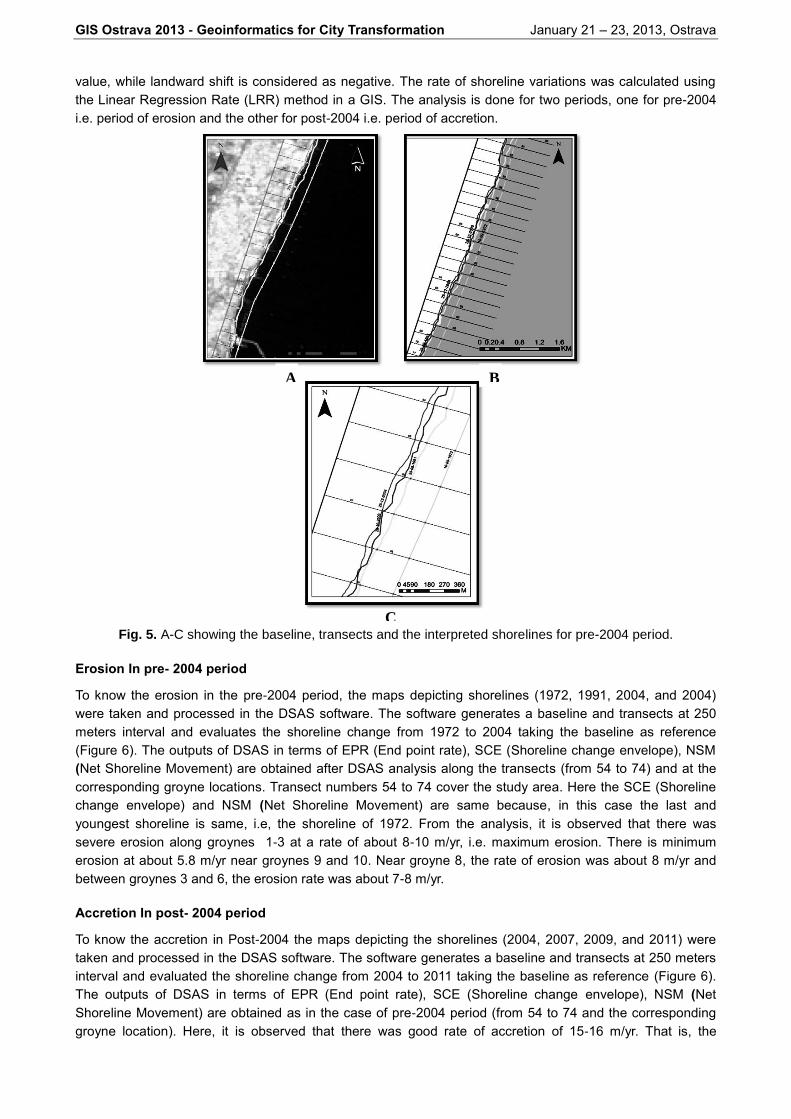
Fig. 5. A-C showing the baseline, transects and the interpreted shorelines for pre-2004 period.
Erosion In pre- 2004 period
To know the erosion in the pre-2004 period, the maps depicting shorelines (1972, 1991, 2004, and 2004)
were taken and processed in the DSAS software. The software generates a baseline and transects at 250
meters interval and evaluates the shoreline change from 1972 to 2004 taking the baseline as reference
(Figure 6). The outputs of DSAS in terms of EPR (End point rate), SCE (Shoreline change envelope), NSM
(Net Shoreline Movement) are obtained after DSAS analysis along the transects (from 54 to 74) and at the
corresponding groyne locations. Transect numbers 54 to 74 cover the study area. Here the SCE (Shoreline
change envelope) and NSM (Net Shoreline Movement) are same because, in this case the last and
youngest shoreline is same, i.e, the shoreline of 1972. From the analysis, it is observed that there was
severe erosion along groynes 1-3 at a rate of about 8-10 m/yr, i.e. maximum erosion. There is minimum
erosion at about 5.8 m/yr near groynes 9 and 10. Near groyne 8, the rate of erosion was about 8 m/yr and
between groynes 3 and 6, the erosion rate was about 7-8 m/yr.
Accretion In post- 2004 period
To know the accretion in Post-2004 the maps depicting the shorelines (2004, 2007, 2009, and 2011) were
taken and processed in the DSAS software. The software generates a baseline and transects at 250 meters
interval and evaluated the shoreline change from 2004 to 2011 taking the baseline as reference (Figure 6).
The outputs of DSAS in terms of EPR (End point rate), SCE (Shoreline change envelope), NSM (Net
Shoreline Movement) are obtained as in the case of pre-2004 period (from 54 to 74 and the corresponding
groyne location). Here, it is observed that there was good rate of accretion of 15-16 m/yr. That is, the
Bay
of
Ben
gal
A B
C
GIS Ostrava 2013 - Geoinformatics for City Transformation January 21 – 23, 2013, Ostrava
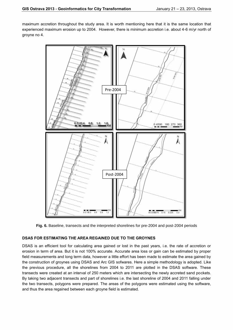
maximum accretion throughout the study area. It is worth mentioning here that it is the same location that
experienced maximum erosion up to 2004. However, there is minimum accretion i.e. about 4-6 m/yr north of
groyne no 4.
Fig. 6. Baseline, transects and the interpreted shorelines for pre-2004 and post-2004 periods
DSAS FOR ESTIMATING THE AREA REGAINED DUE TO THE GROYNES
DSAS is an efficient tool for calculating area gained or lost in the past years, i.e. the rate of accretion or
erosion in term of area. But it is not 100% accurate. Accurate area loss or gain can be estimated by proper
field measurements and long term data, however a little effort has been made to estimate the area gained by
the construction of groynes using DSAS and Arc GIS sofwares. Here a simple methodology is adopted. Like
the previous procedure, all the shorelines from 2004 to 2011 are plotted in the DSAS software. These
transects were created at an interval of 250 meters which are intersecting the newly accreted sand pockets.
By taking two adjacent transects and part of shorelines i.e. the last shoreline of 2004 and 2011 falling under
the two transects, polygons were prepared. The areas of the polygons were estimated using the software,
and thus the area regained between each groyne field is estimated.
Pre-2004
Post-2004

GIS Ostrava 2013 - Geoinformatics for City Transformation January 21 – 23, 2013, Ostrava
Table 3. DSAS estimated area gained between 2004 and 2011 along the groyne fields
FUTURE SHORELINE PREDICTION MODEL USING EPR AND LRR
For the current study, the shoreline data from multi-temporal satellite images and the DSAS software-derived
linear transgression rate are used to prepare a future shoreline prediction model. The end point rate (epr) is
calculated by dividing the distance of shoreline movement by the time elapsed between the earliest and
latest measurements (i.e., the oldest and the most recent shoreline). The major advantage of the EPR is its
ease of computation and minimal requirement for shoreline data (two shorelines). The major disadvantage is
that in cases where more than two shorelines are available, the information about shoreline behavior
provided by additional shorelines is neglected. Thus, changes in sign or magnitude of the shoreline
movement trend, or cyclicity of behavior may be missed. The End Point rate (EPR) method is based on an
empirical equation which shows that the future position of a shoreline can be derived by a linear relationship
between past shoreline positions and time. The change rate (m) and intercept (c) involved in this model are
derived by a line (y = mx+c) extracted from the points on the earliest and latest available shorelines (y and x
represent the shoreline position and time respectively) (USGS, 2005).
Fig. 7. Graphs showing the predicted shoreline positions at three example-transects (54, 55, 58)
Groyne fields 8-9 7-8 6-7 3-5 1-3
Area (Sq.m) 74,458 73,074 35,660 66,129 94,465

GIS Ostrava 2013 - Geoinformatics for City Transformation January 21 – 23, 2013, Ostrava
Fig. 8. Future shoreline positions near, A- Thiruvattriyur B - Royapuram
A linear regression rate-of-change statistic can be determined by fitting a least-squares regression line to all
shoreline points for a particular transect. The regression line is placed so that the sum of the squared
residuals (determined by squaring the offset distance of each data point from the regression line and adding
the squared residuals together) is minimized. The linear regression rate is the slope of the line. The method
of linear regression includes these features: (1) All the data are used, regardless of changes in trend or
accuracy, (2) The method is purely computational, (3) The calculation is based on accepted statistical
concepts, and (4) The method is easy to employ (Dolan et al. 1991).
Graphs are prepared for each transect (from transect no 54- 74) derived by DSAS analysis by using the
mathematical formulae where in x-axis the years and y-axis shows the distance of shoreline from the
baseline. A few examples of the graphs are shown in Figure 7. By plotting the years 2015, 2020, 2025, and
2030 in the graph, the distance of the shoreline can be predicted for each year in the future. The values
obtained from the graphs are plotted in a GIS software to get the future shoreline positions for the years
2015, 2020, 2025 and 2030. Such predicted shorelines are shown in Figure 8.
A
B

GIS Ostrava 2013 - Geoinformatics for City Transformation January 21 – 23, 2013, Ostrava
CONCLUSIONS
We are very much aware of the fact that coastlines are dynamic and they have been changing as long as
there have been coastlines. This statement is very well applicable to the city of Chennai also. The population
of Chennai has grown over the years, and the demand for seaside land and the related development has
increased. Given the magnitude of the wind and wave forces active along the Chennai coast, the
government has adopted several measures of defence mainly in the form of constructing groynes since 2004
to arrest the ongoing erosion and regain the land lost to the sea over the past century. Though it can be
argued that attempts to contain the sea may be futile, it is witnessed here that the groynes are performing
well.
The study presented in this paper has demonstrated that remote sensing and GIS are potential tools for
monitoring the status of coastal cities, especially those undergoing erosion. This paper has demonstrated the
applicability of multispectral satellite images to monitor both erosion and accretion that the Chennai coast
has witnessed in the past. Despite the limitation offered by coarse resolution images in the early 70’s and
80’s, near accurate depiction of the shoreline was done and the changes are also accurately estimated. This
study, carried out in Chennai city indicates that the ten groynes constructed by the government are
performing well by arresting erosion and enhancing accretion, thereby promoting the re-growth of the
shoreline.
Based on the shoreline obtained from multi-temporal satellite images, it may be inferred that alarming rate of
erosion witnessed by the coast up to 2004 has considerably reduced and the process of accretion began in
2004 with an appreciable rate.
The DSAS module, which has taken an input from satellite remote sensing has also yielded adequate
information about the rates of erosion and accretion at different places. Accretion, as analysed by satellite
images and by USGS-DSAS model is certainly very active in most of the groyne-field areas. A maximum of
94465 sq m of land has been gained in the southern part of the study area (near Royapuram), while a
minimum 35660 sq m in the central part of the study area and on an average, 68757 sq m of land has been
regained between 2004 and 2011. Such a rate of accretion will lead to a better landscape along the Chennai
coast and the people will have a better life in the future.
REFERENCES
EARSeL (2002) Observing our environment from space: new solutions for a new millennium. A. A.
Balakema. ISBN 90-5809-254-2.
ICMAM(2005) Shoreline Management Plan for Ennore Coast (Tamilnadu). Report of Integrated Coastal and
Marine Area Management Project Directorate, Ministry of Earth Sciences, India.
Kudale, M.D. (2010). Impact of port development on the coastline and the need for protection. Indian Journal
of Geo-Marine Sciences. Vol 39 (4), pp-597-604.
The Hindu, http://www.thehindu.com/news/cities/chennai/article3413028.ece May 13, 2012
Thieler, E.R., Himmelstoss, E.A., Zichichi, J.L., and Ergul, Ayhan, (2008) Digital Shoreline Analysis System
(DSAS) version 4.0—An ArcGIS extension for calculating shoreline change: U.S. Geological Survey
Open-File Report 2008-1278.
USGS (2005) User Guide and Tutorial for the Extension for ArcGIS v.9.0 (DSAS) version 3.2 Digital
Shoreline Analysis System Part of USGS Open-File Report 2005-1304.
Wang, Y. (1998) Sea-level changes, human impact and coastal responses in China. Journal of Coastal
Research, 14(1), 31-36. ISSN 0749-0208.
Xia, D.X., Wang, W.H., Wu, G.Q., Cui, J.R., Li, F.L. (1993) Coastal erosion in China. Acta Geographica
Sinica, 48: pp: 468-476.
Yu, Ji-Tao; Chen, Zi-Shen (2011) Study on headland-bay sandy coast stability in south China coasts. China
Ocean Engineering, volume 25, issue 1, pp.1-13.