Remote compositional analysis of lunar olivine rich ...sbesse/REPRINTS/Isaacson_M3olivine_2011.pdf · Remote compositional analysis of lunar olivine‐rich lithologies with Moon Mineralogy

Remote compositional analysis of lunar olivine‐rich lithologieswith Moon Mineralogy Mapper (M3) spectra

Peter J. Isaacson,1 Carle M. Pieters,1 Sebastien Besse,2 Roger N. Clark,3 James W. Head,1

Rachel L. Klima,4 John F. Mustard,1 Noah E. Petro,5 Matthew I. Staid,6

Jessica M. Sunshine,2 Lawrence A. Taylor,7 Kevin G. Thaisen,7 and Stefanie Tompkins8

Received 31 August 2010; revised 6 January 2011; accepted 18 January 2011; published 26 April 2011.

[1] A systematic approach for deconvolving remotely sensed lunar olivine‐rich visibleto near‐infrared (VNIR) reflectance spectra with the Modified Gaussian Model (MGM)is evaluated with Chandrayaan‐1 Moon Mineralogy Mapper (M3) spectra. Whereasearlier studies of laboratory reflectance spectra focused only on complications due tochromite inclusions in lunar olivines, we develop a systematic approach for addressing(through continuum removal) the prominent continuum slopes common to remotely sensedreflectance spectra of planetary surfaces. We have validated our continuum removal on asuite of laboratory reflectance spectra. Suites of olivine‐dominated reflectance spectrafrom a small crater near Mare Moscoviense, the Copernicus central peak, Aristarchus, andthe crater Marius in the Marius Hills were analyzed. Spectral diversity was detected invisual evaluation of the spectra and was quantified using the MGM. The MGM‐derivedband positions are used to estimate the olivine’s composition in a relative sense. Spectraof olivines from Moscoviense exhibit diversity in their absorption features, and thisdiversity suggests some variation in olivine Fe/Mg content. Olivines from Copernicus areobserved to be spectrally homogeneous and thus are predicted to be more compositionallyhomogeneous than those at Moscoviense but are of broadly similar composition to theMoscoviense olivines. Olivines from Aristarchus and Marius exhibit clear spectraldifferences from those at Moscoviense and Copernicus but also exhibit features thatsuggest contributions from other phases. If the various precautions discussed here areweighed carefully, the methods presented here can be used to make general predictionsof absolute olivine composition (Fe/Mg content).

Citation: Isaacson, P. J., et al. (2011), Remote compositional analysis of lunar olivine‐rich lithologieswith Moon Mineralogy Mapper (M3) spectra, J. Geophys. Res., 116, E00G11, doi:10.1029/2010JE003731.

1. Introduction

[2] The mineralogy and mineral composition of planetarysamples contain a rich record of the thermal and chemicalevolution of the planetary body. The processes responsiblefor the cooling of planetary bodies include magma oceanformation and solidification, differentiation (density strati-

fication) and overturn, large‐scale convection, and volcanicactivity. These processes all produce distinct signatures inthe mineral assemblages and compositions produced acrossa range of depths and across the body’s surface. While therecord can be complex, the composition and mineralogy ofplanetary samples represent one of the most powerful toolsavailable for unraveling the geologic history of a planetarybody. While returned samples are the most powerful tool forevaluating planetary composition and mineralogy, remotesensing, such as with orbital visible to near‐infrared (VNIR)reflectance spectroscopy, offers a number of advantages.These advantages include global coverage (if conductedfrom orbit) and the ability to analyze composition withoutreturned samples, although such remote measurements aregreatly strengthened by the context and ground truth pro-vided by returned samples [e.g., Pieters, 1999; Taylor et al.,2001, 2010].[3] Olivine in particular is a useful mineral with which to

evaluate the geologic evolution of igneous planetary bodiessuch as the Moon. Olivine is typically one of the firstminerals to crystallize from a mafic magma, and its com-position is indicative of the composition and degree of

1Department of Geological Sciences, Brown University, Providence,Rhode Island, USA.

2Astronomy Department, University of Maryland, College Park,Maryland, USA.

3U.S. Geological Survey, Denver, Colorado, USA.4Johns Hopkins University Applied Physics Laboratory, Laurel,

Maryland, USA.5NASA Goddard Space Flight Center, Greenbelt, Maryland, USA.6Planetary Science Institute, Tucson, Arizona, USA.7Planetary Geosciences Institute, University of Tennessee, Knoxville,

Tennessee, USA.8Defense Advanced Research Projects Agency, Arlington, Virginia,

USA.

Copyright 2011 by the American Geophysical Union.0148‐0227/11/2010JE003731

JOURNAL OF GEOPHYSICAL RESEARCH, VOL. 116, E00G11, doi:10.1029/2010JE003731, 2011

E00G11 1 of 17

http://dx.doi.org/10.1029/2010JE003731

evolution of the source region in the case of a primarymagma [Basaltic Volcanism Study Project (BVSP), 1981].Recent results suggest that olivine is exposed largely in andaround the rims of large lunar impact basins [Yamamotoet al., 2010]. Such regions should represent some of thedeepest materials excavated by the basin‐forming impact.Yamamoto et al. [2010] argued that these olivine detectionsmay represent exposures of the lunar mantle, but could alsorepresent differentiated plutons resulting from secondarymagmatic intrusions into the lunar crust. Yamamoto et al.[2010] favor the mantle source model as the more probableinterpretation, based primarily on an apparent lack of pla-gioclase association with the olivine exposures. However,many of the detections are associated with exposures of“pure anorthosite” reported by Ohtake et al. [2009], andplagioclase is difficult to detect in the near‐infrared whenmixed with absorbing mafic minerals like pyroxene andolivine. While the detection of the olivine signature is criti-cal, the composition of those olivines is an important addi-tional clue to the olivine’s source and history, as mantleolivines would be expected to be quite Mg‐rich.[4] Generally, for primary magmas, forsteritic (high Mg #

(molar Mg/Mg+Fe)) olivine is indicative of a primitivesource, and more fayalitic (low Mg #) olivine is indicative ofa more evolved source [BVSP, 1981]. Lunar samples containolivine of diverse compositions, from very Mg‐rich (∼Fo90)in Mg suite rocks to more Fe‐rich in basalts; olivines inbasalts that are sufficiently abundant (>1–2 modal %) to bedetectable through remote VNIR reflectance spectroscopygenerally range from <Fo80 to ∼Fo50 [e.g., Papike et al.,1998]. Additionally, olivine has a distinctive signature inVNIR reflectance spectra, and this signature is composi-tionally dependent, meaning that remotely sensed VNIRreflectance spectra are sensitive to both the presence andcomposition of olivine on planetary surfaces [Burns, 1970;

King and Ridley, 1987; Sunshine and Pieters, 1998; Dyaret al., 2009]. Typical olivine spectra have a broad, com-posite absorption feature centered near 1050 nm. Theseabsorptions are caused by electronic transitions in Fe2+ ionslocated in distorted octahedral crystallographic sites. Thecentral absorption is caused by Fe2+ in the M2 site, while thetwo exterior absorptions are caused by Fe2+ in the M1 site[Burns, 1970; Burns et al., 1972; Burns, 1974, 1993]. Anexample olivine spectrum is plotted in Figure 1, whichshows the spectrum of San Carlos olivine (∼Fo90), acommon laboratory standard due to its composition andrelative purity. The three component absorptions that pro-duce the composite absorption feature are labeled with theFe2+‐bearing crystallographic site responsible for thecomponent absorption.[5] The properties of the three component absorptions are

a function of the olivine’s Mg #, and shift in regular, well‐characterized ways with changing Mg # [Sunshine andPieters, 1998]. When olivine spectra are deconvolved withquantitative techniques such as the Modified GaussianModel (MGM), the MGM‐derived band parameters of theindividual component absorptions can be used to estimatethe olivine’s composition [Sunshine et al., 1990; Sunshineand Pieters, 1998]. As demonstrated by previous work,these MGM‐derived parameters can be applied to solve forolivine composition as a function of band position [Sunshineand Pieters, 1998; Isaacson and Pieters, 2010]. The relativestrengths, and to a lesser extent, widths of the three com-ponent absorptions also shift with changing olivine Mg #,although this trend is less useful for compositional analysis.[6] Compositional analysis of lunar olivines with VNIR

reflectance spectroscopy is complicated by the presence ofinclusions of Cr‐spinel (largely chromite), which causesabsorptions beyond ∼1600 nm [Cloutis et al., 2004;Isaacson and Pieters, 2010]. Inclusion‐free olivine spectraare bright and featureless across this wavelength region, aproperty which was used to define a standard approach todeconvolutions of olivine spectra [Sunshine and Pieters,1998]. The absorptions due to Cr‐spinel inclusions, com-mon in lunar olivines, cause the results of MGM decon-volutions of lunar olivine spectra to be inconsistent withdeconvolutions of terrestrial olivine spectra of similar com-position [Papike et al., 1998; Isaacson and Pieters, 2010].Because the terrestrial olivine spectra deconvolutions are thebasis of the trends used for compositional predictions,Chromite‐bearing lunar olivines require a modified approachtoMGM deconvolutions. Such a modified approach has beendeveloped by Isaacson and Pieters [2010], and involvestruncating the olivine spectra to focus only on the 1000 nmregion, as well as enforcing a flat (slope value of 0) con-tinuum slope. This approach was able to reproduce thetrends determined through analysis of terrestrial spectralacking Cr‐spinel absorptions [Sunshine and Pieters, 1998]to within ∼5–10% accuracy. In addition to the Cr‐spinelinclusions, lunar olivines studied with remote sensing maybe affected by mixing with pyroxene. Pyroxene will intro-duce additional absorptions that complicate substantiallydeconvolutions of the composite olivine 1000 nm feature.Pyroxene and mixtures are discussed more thoroughly insection 5.2.3.[7] The study by Isaacson and Pieters [2010] identified

two major complications in compositional analyses of lunar

Figure 1. Bidirectional reflectance spectrum of San Carlosolivine (∼Fo90). The component absorptions that comprisethe composite olivine 1000 nm absorption feature arelabeled with the Fe2+‐bearing site responsible for the com-ponent absorption. Note the bright, featureless nature ofthe spectrum beyond ∼1500 nm.

ISAACSON ET AL.: ANALYSIS OF LUNAR OLIVINES WITH M3 E00G11E00G11

2 of 17

olivines with remotely sensed VNIR reflectance spectra: thelong‐wavelength absorptions caused by chromite inclusionsand the effect of continuum slopes common to remotelysensed spectra of planetary surfaces. Isaacson and Pieters[2010] addressed the former complication but explicitlydid not address the latter, limiting their analyses to laboratoryreflectance spectra in which flat continuum slopes areappropriate. In this study, we extend the Isaacson and Pieters[2010] approach to address the effect of continuum slopes.We propose a method for standardizing the continuum slopeused to deconvolve remotely sensed olivine spectra, andevaluate the effect of this method on the established trendsin MGM‐derived band position found in both terrestrialolivine and chromite‐bearing lunar olivine spectra. Weapply this approach to predict olivine compositions fromseveral locations on the lunar surface using VNIR reflec-tance spectra collected by the Moon Mineralogy Mapper(M3) on Chandrayaan‐1 from several locations on the lunarsurface.

2. Background: The Moon Mineralogy Mapper

[8] The Moon Mineralogy Mapper is an imaging spec-trometer covering visible to near‐infrared wavelengths. Itwas a guest instrument on the Indian Space ResearchOrganisation (ISRO) Chandrayaan‐1 mission. M3 collectedglobal data in 85 spectral channels from 400–3000 nm at aspatial resolution of 140 m/pixel from a 100 km orbit. Morecomplete descriptions of the M3 instrument are provided byPieters et al. [2009, 2011]. A description of the calibrationof M3 data is provided by R. O. Green et al. (The MoonMineralogy Mapper (M3) imaging spectrometer for lunarscience: Instrument, calibration, and on‐orbit measurementperformance, submitted to Journal of Geophysical Research,2011), and a description of the operational history and spatialcoverage of M3 is provided by Boardman et al. [2011].

3. Methods

3.1. Variable Continuum Slopes: Continuum Removal

[9] Continuum slopes in remotely sensed spectra arehighly variable, as they can be influenced by a number ofparameters, including surface texture, grain size, viewinggeometry, and alteration such as through the process ofspace weathering. On the Moon, continuum slopes arepredominantly affected by the presence of vapor‐depositednanophase iron‐bearing rims on grains of lunar soil [e.g.,Pieters et al., 2000; Hapke, 2001; Taylor et al., 2001; Nobleet al., 2005, 2007; Taylor et al., 2010]. The optical effects ofthis nanophase iron are complex, but one of the majoreffects is an increase in the slope of the continuum (i.e.,“red” continuum slopes). This effect becomes more pro-nounced with increasing degree of weathering [e.g., Pieterset al., 2000; Noble et al., 2001]. Even relatively immaturematerials on the Moon exhibit moderately “red” continuumslopes. Prominent continuum slopes cause shifts in apparentband center [e.g., Clark and Roush, 1984; Clark, 1999].Thus, flat continuum slopes such as those used in previoussystematic treatments of olivine reflectance spectra will notbe practical for the majority of remotely sensed spectracollected of the lunar surface.

[10] The ubiquitous but variable nature of continuumslopes in remotely sensed VNIR reflectance spectra ofplanetary surfaces is a major complication in quantitativeanalysis of diagnostic absorption features present in thosespectra. To treat these variable continuum slopes fully withan MGM‐based approach, the continuum for each individ-ual spectrum analyzed must be modeled individually foreach fit [e.g., Sunshine and Pieters, 1998; Sunshine et al.,2007]. While this is the most rigorous method to treatcontinuum slopes, the drawback of this approach is theadditional complexity of the models and the potential vari-able methods applied to individual spectra. This variabilitycan introduce more sources of error into comparisonsbetween model results. To avoid these complexities andsources of error, we chose to use a systematic approach thatwill enable comparisons between model results more read-ily. We employ the approach developed by Isaacson andPieters [2010] (truncating spectra and enforcing flat con-tinuum slopes), but we include additional steps to address,in a systematic way, spectra for which flat continuum slopesare not practical.[11] Our approach to dealing with continuum slopes is to

remove the continuum slope prior to conducting MGM fits.This differs from the traditional MGM approach in whichthe continuum is modeled concurrently with the absorptions.Because the continuum is removed prior to performingdeconvolutions, the slope (first‐order polynomial term in theexpression of the continuum slope) is fixed at zero for thedeconvolutions, with only the offset (zero‐order term)allowed to vary. We make a simplifying assumption that therelative trends in band position with olivine compositionestablished from terrestrial olivines [Sunshine and Pieters,1998] remain valid after continuum removal. However, itis beyond the scope of this project to verify that the effect ofthe continuum slope on band position is constant across allolivine compositions. Our goal in simplifying the modelingof the continuum slope is to ensure that we can apply ourmethods in a consistent manner regardless of the nature andmagnitude of the continuum slope in any given spectrum. Itis possible that our simplifications may introduce newbiases, particularly if the effect of continuum removal iscomposition dependent. The advantage of this approach isthat our methods can be replicated easily and consistently.However, a disadvantage of this approach is the inability tocompare the resulting deconvolutions to existing deconvo-lutions of laboratory lunar olivine spectra performed withoutcontinuum removal. Thus, although the trends in bandposition with olivine composition are assumed to be valid ina relative sense, we cannot use our deconvolutions to assignabsolute olivine compositions. A direct comparison to lab-oratory spectra would require substantial new laboratorywork, including a reanalysis of the full suite of terrestriallaboratory olivine reflectance spectra with this new approachto modeling the continuum.[12] The continuum slope to be removed is determined by

fitting a local continuum over the principle olivine absorp-tion feature. This local continuum slope is determined bytangent points on the short‐ and long‐wavelength side of theabsorption. Our method is to pick the “high reflectance”points on either side of the absorption as the tangent points.In our experience, the long‐wavelength inflection pointtypically falls near ∼1700 nm, while the short‐wavelength


3 of 17

inflection point is more variable. We evaluated continuumslope tangent points optimized for each spectrum as well asfixed tangent points for all spectra. We also evaluatedvarious combinations of fixed and optimized tangentpoints (e.g., optimized short‐wavelength point, fixed long‐wavelength point for all spectra). While the differences aregenerally slight, we found that the results most consistent withestablished parameter ranges for olivine were obtained withshort‐wavelength tangent points optimized for each spectrum(though typically ∼730–770 nm) and fixed long‐wavelengthtangent points at 1700 nm. Once obtained, the local continuumslope is “removed” by dividing the original spectrum by thelocal continuum. After performing the continuum removalbased on these local continuum slopes, MGM fits are con-ducted as described by Isaacson and Pieters [2010]. As in theIsaacson and Pieters [2010] approach, in fitting a particularspectrum, multiple starting points are used to ensure that a“global” optimum fit is achieved. We employ the standardstarting points presented by Isaacson and Pieters [2010],varying only the offset of the continuum slope in the startingmodels to a more reasonable value for continuum‐removedspectra, which intersect zero in log reflectance space.

3.2. Effect of Continuum Removal: Laboratory Spectra

[13] We evaluate the robustness of the continuum removalprocess by analyzing its effect on deconvolutions of labo-ratory olivine reflectance spectra. The spectra used for thesecontinuum removal analyses are a series of San Carlosolivine subsamples subjected to pulsed laser irradiation ofvarying intensity in an attempt to simulate the spaceweathering process [Yamada et al., 1999; Sasaki et al.,

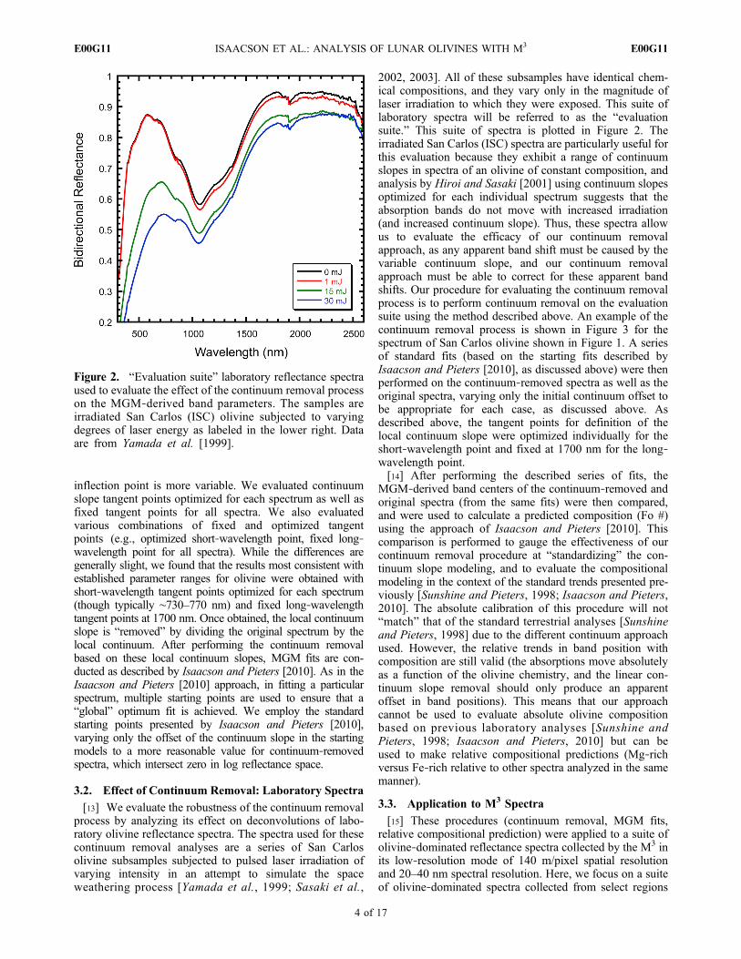
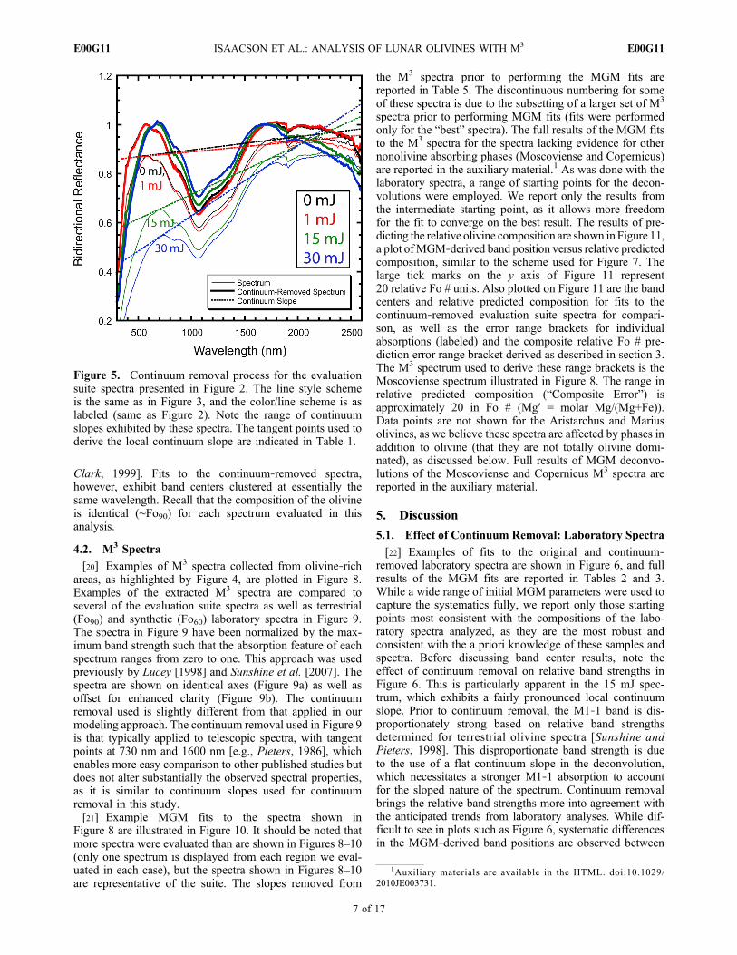
2002, 2003]. All of these subsamples have identical chem-ical compositions, and they vary only in the magnitude oflaser irradiation to which they were exposed. This suite oflaboratory spectra will be referred to as the “evaluationsuite.” This suite of spectra is plotted in Figure 2. Theirradiated San Carlos (ISC) spectra are particularly useful forthis evaluation because they exhibit a range of continuumslopes in spectra of an olivine of constant composition, andanalysis by Hiroi and Sasaki [2001] using continuum slopesoptimized for each individual spectrum suggests that theabsorption bands do not move with increased irradiation(and increased continuum slope). Thus, these spectra allowus to evaluate the efficacy of our continuum removalapproach, as any apparent band shift must be caused by thevariable continuum slope, and our continuum removalapproach must be able to correct for these apparent bandshifts. Our procedure for evaluating the continuum removalprocess is to perform continuum removal on the evaluationsuite using the method described above. An example of thecontinuum removal process is shown in Figure 3 for thespectrum of San Carlos olivine shown in Figure 1. A seriesof standard fits (based on the starting fits described byIsaacson and Pieters [2010], as discussed above) were thenperformed on the continuum‐removed spectra as well as theoriginal spectra, varying only the initial continuum offset tobe appropriate for each case, as discussed above. Asdescribed above, the tangent points for definition of thelocal continuum slope were optimized individually for theshort‐wavelength point and fixed at 1700 nm for the long‐wavelength point.[14] After performing the described series of fits, the

MGM‐derived band centers of the continuum‐removed andoriginal spectra (from the same fits) were then compared,and were used to calculate a predicted composition (Fo #)using the approach of Isaacson and Pieters [2010]. Thiscomparison is performed to gauge the effectiveness of ourcontinuum removal procedure at “standardizing” the con-tinuum slope modeling, and to evaluate the compositionalmodeling in the context of the standard trends presented pre-viously [Sunshine and Pieters, 1998; Isaacson and Pieters,2010]. The absolute calibration of this procedure will not“match” that of the standard terrestrial analyses [Sunshineand Pieters, 1998] due to the different continuum approachused. However, the relative trends in band position withcomposition are still valid (the absorptions move absolutelyas a function of the olivine chemistry, and the linear con-tinuum slope removal should only produce an apparentoffset in band positions). This means that our approachcannot be used to evaluate absolute olivine compositionbased on previous laboratory analyses [Sunshine andPieters, 1998; Isaacson and Pieters, 2010] but can beused to make relative compositional predictions (Mg‐richversus Fe‐rich relative to other spectra analyzed in the samemanner).

3.3. Application to M3 Spectra

[15] These procedures (continuum removal, MGM fits,relative compositional prediction) were applied to a suite ofolivine‐dominated reflectance spectra collected by the M3 inits low‐resolution mode of 140 m/pixel spatial resolutionand 20–40 nm spectral resolution. Here, we focus on a suiteof olivine‐dominated spectra collected from select regions

Figure 2. “Evaluation suite” laboratory reflectance spectraused to evaluate the effect of the continuum removal processon the MGM‐derived band parameters. The samples areirradiated San Carlos (ISC) olivine subjected to varyingdegrees of laser energy as labeled in the lower right. Dataare from Yamada et al. [1999].


4 of 17

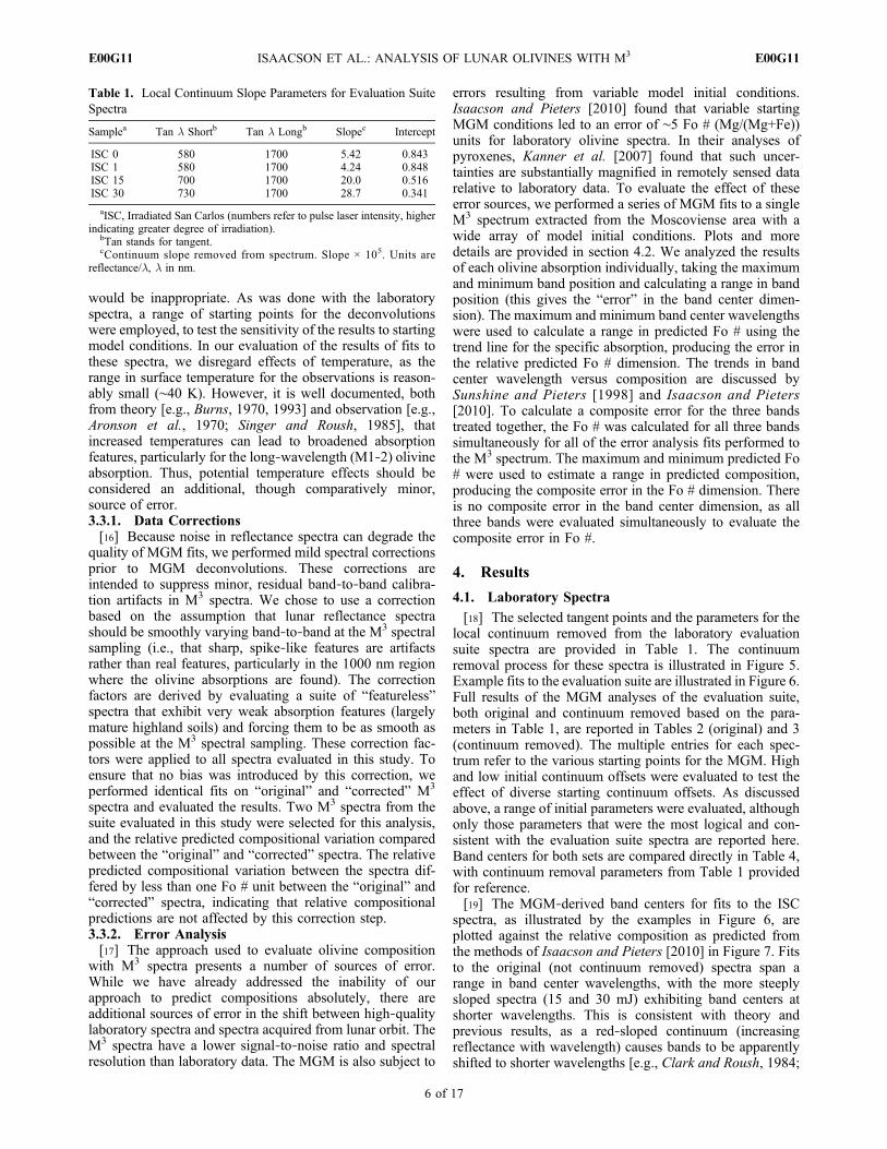
on the lunar surface. These regions include a small craternorthwest of the rim of the Moscoviense basin, theCopernicus central peak, Aristarchus, and Marius crater inthe eastern Marius Hills. Previous studies have identified thepresence of olivine at Copernicus [Pieters, 1982; Pieters andWilhelms, 1985; Lucey et al., 1991; Le Mouélic, 2001;Yamamoto et al., 2010] and Aristarchus [Le Mouélic et al.,1999a; Chevrel et al., 2009; Yamamoto et al., 2010]. TheMoscoviense olivines occur close to exposures of unusualmafic lithologies [Pieters et al., 2011] and may be associatedwith the processes responsible for the production of thoselithologies, although our analyses cannot confirm a geneticrelationship. Olivine‐rich areas were highlighted by using aratio of the integrated band strengths at 1000 and 2000 nm. Inour formulation (1000 nm/2000 nm), spectra with strong1000 nm features and weak 2000 nm features, such as thosedominated by olivine, will have high values in this param-eter. This approach is highlighted in Figure 4, which showsthis parameter mapped in color overlaid on a M3 albedo bandfor context. Two regions are displayed in Figure 4, the smallcrater in the Moscoviense region and Copernicus. Areasshowing up in yellow‐orange‐red colors in this scheme willtend to be olivine‐rich. The olivine spectra from Aristarchusare discussed by Mustard et al. [2011], and those fromMarius are discussed by Besse et al. [2011]. The Aristarchusolivines are located in the southwest rim and ejecta ofAristarchus, and the Marius olivines are located in the floor

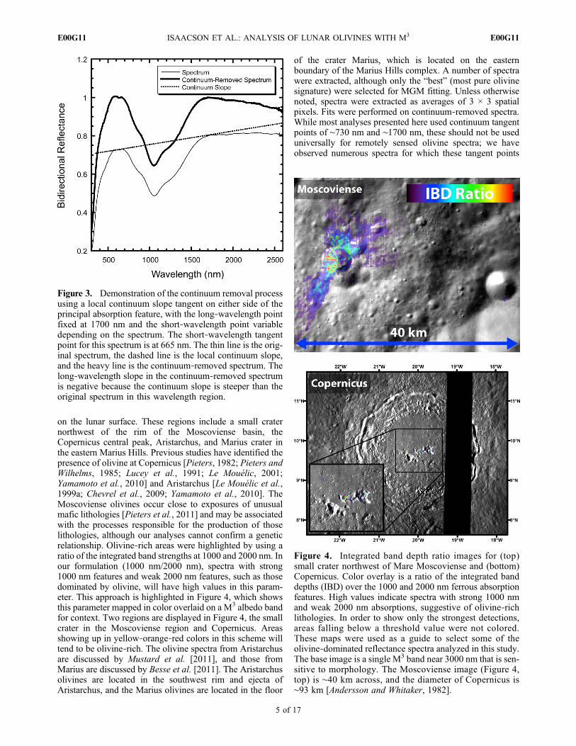
of the crater Marius, which is located on the easternboundary of the Marius Hills complex. A number of spectrawere extracted, although only the “best” (most pure olivinesignature) were selected for MGM fitting. Unless otherwisenoted, spectra were extracted as averages of 3 × 3 spatialpixels. Fits were performed on continuum‐removed spectra.While most analyses presented here used continuum tangentpoints of ∼730 nm and ∼1700 nm, these should not be useduniversally for remotely sensed olivine spectra; we haveobserved numerous spectra for which these tangent points

Figure 3. Demonstration of the continuum removal processusing a local continuum slope tangent on either side of theprincipal absorption feature, with the long‐wavelength pointfixed at 1700 nm and the short‐wavelength point variabledepending on the spectrum. The short‐wavelength tangentpoint for this spectrum is at 665 nm. The thin line is the orig-inal spectrum, the dashed line is the local continuum slope,and the heavy line is the continuum‐removed spectrum. Thelong‐wavelength slope in the continuum‐removed spectrumis negative because the continuum slope is steeper than theoriginal spectrum in this wavelength region.

Figure 4. Integrated band depth ratio images for (top)small crater northwest of Mare Moscoviense and (bottom)Copernicus. Color overlay is a ratio of the integrated banddepths (IBD) over the 1000 and 2000 nm ferrous absorptionfeatures. High values indicate spectra with strong 1000 nmand weak 2000 nm absorptions, suggestive of olivine‐richlithologies. In order to show only the strongest detections,areas falling below a threshold value were not colored.These maps were used as a guide to select some of theolivine‐dominated reflectance spectra analyzed in this study.The base image is a single M3 band near 3000 nm that is sen-sitive to morphology. The Moscoviense image (Figure 4,top) is ∼40 km across, and the diameter of Copernicus is∼93 km [Andersson and Whitaker, 1982].


5 of 17

would be inappropriate. As was done with the laboratoryspectra, a range of starting points for the deconvolutionswere employed, to test the sensitivity of the results to startingmodel conditions. In our evaluation of the results of fits tothese spectra, we disregard effects of temperature, as therange in surface temperature for the observations is reason-ably small (∼40 K). However, it is well documented, bothfrom theory [e.g., Burns, 1970, 1993] and observation [e.g.,Aronson et al., 1970; Singer and Roush, 1985], thatincreased temperatures can lead to broadened absorptionfeatures, particularly for the long‐wavelength (M1‐2) olivineabsorption. Thus, potential temperature effects should beconsidered an additional, though comparatively minor,source of error.3.3.1. Data Corrections[16] Because noise in reflectance spectra can degrade the

quality of MGM fits, we performed mild spectral correctionsprior to MGM deconvolutions. These corrections areintended to suppress minor, residual band‐to‐band calibra-tion artifacts in M3 spectra. We chose to use a correctionbased on the assumption that lunar reflectance spectrashould be smoothly varying band‐to‐band at the M3 spectralsampling (i.e., that sharp, spike‐like features are artifactsrather than real features, particularly in the 1000 nm regionwhere the olivine absorptions are found). The correctionfactors are derived by evaluating a suite of “featureless”spectra that exhibit very weak absorption features (largelymature highland soils) and forcing them to be as smooth aspossible at the M3 spectral sampling. These correction fac-tors were applied to all spectra evaluated in this study. Toensure that no bias was introduced by this correction, weperformed identical fits on “original” and “corrected” M3

spectra and evaluated the results. Two M3 spectra from thesuite evaluated in this study were selected for this analysis,and the relative predicted compositional variation comparedbetween the “original” and “corrected” spectra. The relativepredicted compositional variation between the spectra dif-fered by less than one Fo # unit between the “original” and“corrected” spectra, indicating that relative compositionalpredictions are not affected by this correction step.3.3.2. Error Analysis[17] The approach used to evaluate olivine composition

with M3 spectra presents a number of sources of error.While we have already addressed the inability of ourapproach to predict compositions absolutely, there areadditional sources of error in the shift between high‐qualitylaboratory spectra and spectra acquired from lunar orbit. TheM3 spectra have a lower signal‐to‐noise ratio and spectralresolution than laboratory data. The MGM is also subject to

errors resulting from variable model initial conditions.Isaacson and Pieters [2010] found that variable startingMGM conditions led to an error of ∼5 Fo # (Mg/(Mg+Fe))units for laboratory olivine spectra. In their analyses ofpyroxenes, Kanner et al. [2007] found that such uncer-tainties are substantially magnified in remotely sensed datarelative to laboratory data. To evaluate the effect of theseerror sources, we performed a series of MGM fits to a singleM3 spectrum extracted from the Moscoviense area with awide array of model initial conditions. Plots and moredetails are provided in section 4.2. We analyzed the resultsof each olivine absorption individually, taking the maximumand minimum band position and calculating a range in bandposition (this gives the “error” in the band center dimen-sion). The maximum and minimum band center wavelengthswere used to calculate a range in predicted Fo # using thetrend line for the specific absorption, producing the error inthe relative predicted Fo # dimension. The trends in bandcenter wavelength versus composition are discussed bySunshine and Pieters [1998] and Isaacson and Pieters[2010]. To calculate a composite error for the three bandstreated together, the Fo # was calculated for all three bandssimultaneously for all of the error analysis fits performed tothe M3 spectrum. The maximum and minimum predicted Fo# were used to estimate a range in predicted composition,producing the composite error in the Fo # dimension. Thereis no composite error in the band center dimension, as allthree bands were evaluated simultaneously to evaluate thecomposite error in Fo #.

4. Results

4.1. Laboratory Spectra

[18] The selected tangent points and the parameters for thelocal continuum removed from the laboratory evaluationsuite spectra are provided in Table 1. The continuumremoval process for these spectra is illustrated in Figure 5.Example fits to the evaluation suite are illustrated in Figure 6.Full results of the MGM analyses of the evaluation suite,both original and continuum removed based on the para-meters in Table 1, are reported in Tables 2 (original) and 3(continuum removed). The multiple entries for each spec-trum refer to the various starting points for the MGM. Highand low initial continuum offsets were evaluated to test theeffect of diverse starting continuum offsets. As discussedabove, a range of initial parameters were evaluated, althoughonly those parameters that were the most logical and con-sistent with the evaluation suite spectra are reported here.Band centers for both sets are compared directly in Table 4,with continuum removal parameters from Table 1 providedfor reference.[19] The MGM‐derived band centers for fits to the ISC

spectra, as illustrated by the examples in Figure 6, areplotted against the relative composition as predicted fromthe methods of Isaacson and Pieters [2010] in Figure 7. Fitsto the original (not continuum removed) spectra span arange in band center wavelengths, with the more steeplysloped spectra (15 and 30 mJ) exhibiting band centers atshorter wavelengths. This is consistent with theory andprevious results, as a red‐sloped continuum (increasingreflectance with wavelength) causes bands to be apparentlyshifted to shorter wavelengths [e.g., Clark and Roush, 1984;

Table 1. Local Continuum Slope Parameters for Evaluation SuiteSpectra

Samplea Tan l Shortb Tan l Longb Slopec Intercept

ISC 0 580 1700 5.42 0.843ISC 1 580 1700 4.24 0.848ISC 15 700 1700 20.0 0.516ISC 30 730 1700 28.7 0.341

aISC, Irradiated San Carlos (numbers refer to pulse laser intensity, higherindicating greater degree of irradiation).

bTan stands for tangent.cContinuum slope removed from spectrum. Slope × 105. Units are

reflectance/l, l in nm.


6 of 17

Clark, 1999]. Fits to the continuum‐removed spectra,however, exhibit band centers clustered at essentially thesame wavelength. Recall that the composition of the olivineis identical (∼Fo90) for each spectrum evaluated in thisanalysis.

4.2. M3 Spectra

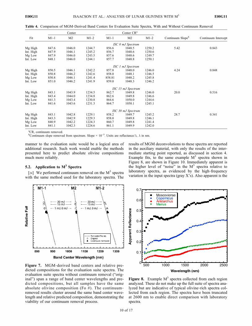
[20] Examples of M3 spectra collected from olivine‐richareas, as highlighted by Figure 4, are plotted in Figure 8.Examples of the extracted M3 spectra are compared toseveral of the evaluation suite spectra as well as terrestrial(Fo90) and synthetic (Fo60) laboratory spectra in Figure 9.The spectra in Figure 9 have been normalized by the max-imum band strength such that the absorption feature of eachspectrum ranges from zero to one. This approach was usedpreviously by Lucey [1998] and Sunshine et al. [2007]. Thespectra are shown on identical axes (Figure 9a) as well asoffset for enhanced clarity (Figure 9b). The continuumremoval used is slightly different from that applied in ourmodeling approach. The continuum removal used in Figure 9is that typically applied to telescopic spectra, with tangentpoints at 730 nm and 1600 nm [e.g., Pieters, 1986], whichenables more easy comparison to other published studies butdoes not alter substantially the observed spectral properties,as it is similar to continuum slopes used for continuumremoval in this study.[21] Example MGM fits to the spectra shown in

Figure 8 are illustrated in Figure 10. It should be noted thatmore spectra were evaluated than are shown in Figures 8–10(only one spectrum is displayed from each region we eval-uated in each case), but the spectra shown in Figures 8–10are representative of the suite. The slopes removed from

the M3 spectra prior to performing the MGM fits arereported in Table 5. The discontinuous numbering for someof these spectra is due to the subsetting of a larger set of M3

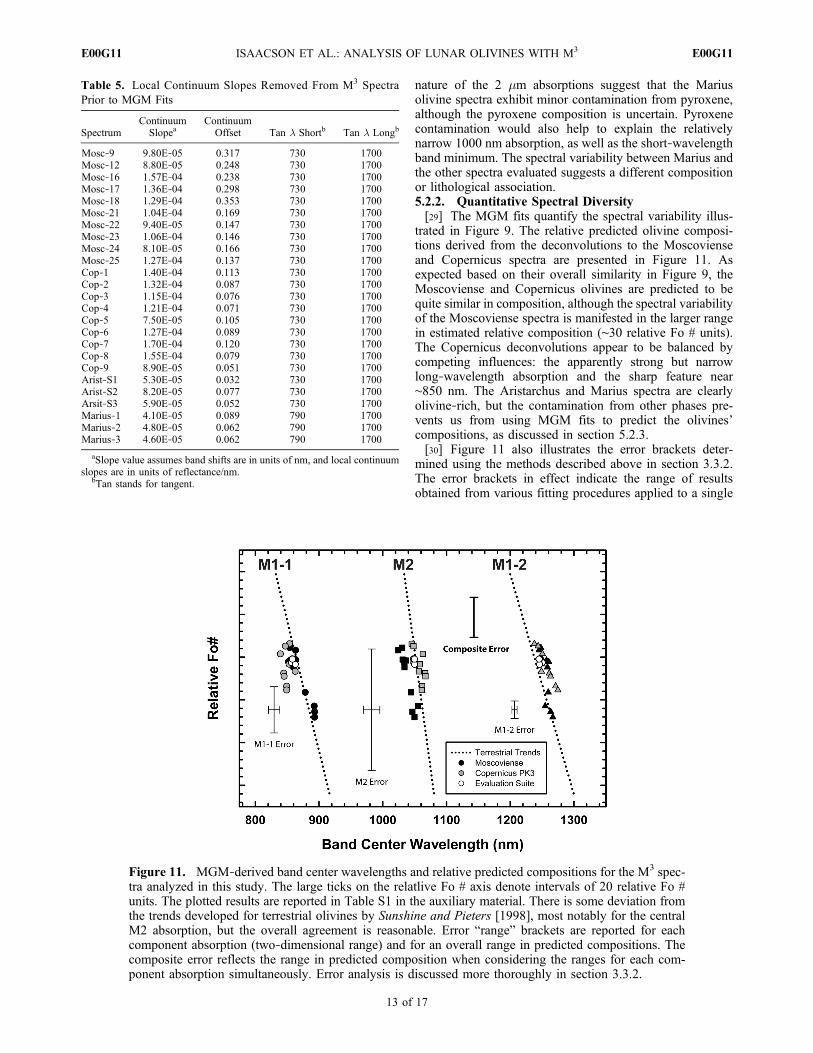
spectra prior to performing MGM fits (fits were performedonly for the “best” spectra). The full results of the MGM fitsto the M3 spectra for the spectra lacking evidence for othernonolivine absorbing phases (Moscoviense and Copernicus)are reported in the auxiliary material.1 As was done with thelaboratory spectra, a range of starting points for the decon-volutions were employed. We report only the results fromthe intermediate starting point, as it allows more freedomfor the fit to converge on the best result. The results of pre-dicting the relative olivine composition are shown in Figure 11,a plot ofMGM‐derived band position versus relative predictedcomposition, similar to the scheme used for Figure 7. Thelarge tick marks on the y axis of Figure 11 represent20 relative Fo # units. Also plotted on Figure 11 are the bandcenters and relative predicted composition for fits to thecontinuum‐removed evaluation suite spectra for compari-son, as well as the error range brackets for individualabsorptions (labeled) and the composite relative Fo # pre-diction error range bracket derived as described in section 3.The M3 spectrum used to derive these range brackets is theMoscoviense spectrum illustrated in Figure 8. The range inrelative predicted composition (“Composite Error”) isapproximately 20 in Fo # (Mg′ = molar Mg/(Mg+Fe)).Data points are not shown for the Aristarchus and Mariusolivines, as we believe these spectra are affected by phases inaddition to olivine (that they are not totally olivine domi-nated), as discussed below. Full results of MGM deconvo-lutions of the Moscoviense and Copernicus M3 spectra arereported in the auxiliary material.

5. Discussion

5.1. Effect of Continuum Removal: Laboratory Spectra

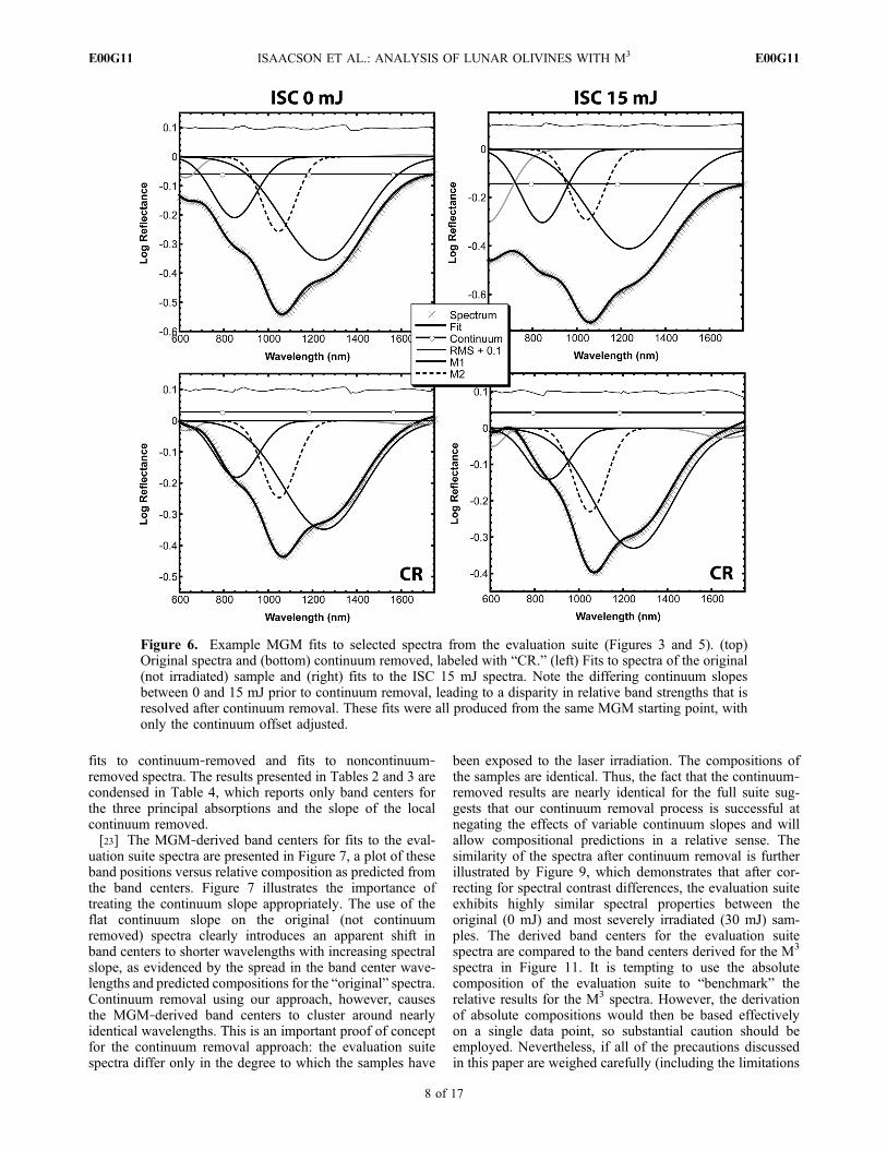
[22] Examples of fits to the original and continuum‐removed laboratory spectra are shown in Figure 6, and fullresults of the MGM fits are reported in Tables 2 and 3.While a wide range of initial MGM parameters were used tocapture the systematics fully, we report only those startingpoints most consistent with the compositions of the labo-ratory spectra analyzed, as they are the most robust andconsistent with the a priori knowledge of these samples andspectra. Before discussing band center results, note theeffect of continuum removal on relative band strengths inFigure 6. This is particularly apparent in the 15 mJ spec-trum, which exhibits a fairly pronounced local continuumslope. Prior to continuum removal, the M1‐1 band is dis-proportionately strong based on relative band strengthsdetermined for terrestrial olivine spectra [Sunshine andPieters, 1998]. This disproportionate band strength is dueto the use of a flat continuum slope in the deconvolution,which necessitates a stronger M1‐1 absorption to accountfor the sloped nature of the spectrum. Continuum removalbrings the relative band strengths more into agreement withthe anticipated trends from laboratory analyses. While dif-ficult to see in plots such as Figure 6, systematic differencesin the MGM‐derived band positions are observed between

Figure 5. Continuum removal process for the evaluationsuite spectra presented in Figure 2. The line style schemeis the same as in Figure 3, and the color/line scheme is aslabeled (same as Figure 2). Note the range of continuumslopes exhibited by these spectra. The tangent points used toderive the local continuum slope are indicated in Table 1.

1Auxiliary materials are available in the HTML. doi:10.1029/2010JE003731.


7 of 17

fits to continuum‐removed and fits to noncontinuum‐removed spectra. The results presented in Tables 2 and 3 arecondensed in Table 4, which reports only band centers forthe three principal absorptions and the slope of the localcontinuum removed.[23] The MGM‐derived band centers for fits to the eval-

uation suite spectra are presented in Figure 7, a plot of theseband positions versus relative composition as predicted fromthe band centers. Figure 7 illustrates the importance oftreating the continuum slope appropriately. The use of theflat continuum slope on the original (not continuumremoved) spectra clearly introduces an apparent shift inband centers to shorter wavelengths with increasing spectralslope, as evidenced by the spread in the band center wave-lengths and predicted compositions for the “original” spectra.Continuum removal using our approach, however, causesthe MGM‐derived band centers to cluster around nearlyidentical wavelengths. This is an important proof of conceptfor the continuum removal approach: the evaluation suitespectra differ only in the degree to which the samples have

been exposed to the laser irradiation. The compositions ofthe samples are identical. Thus, the fact that the continuum‐removed results are nearly identical for the full suite sug-gests that our continuum removal process is successful atnegating the effects of variable continuum slopes and willallow compositional predictions in a relative sense. Thesimilarity of the spectra after continuum removal is furtherillustrated by Figure 9, which demonstrates that after cor-recting for spectral contrast differences, the evaluation suiteexhibits highly similar spectral properties between theoriginal (0 mJ) and most severely irradiated (30 mJ) sam-ples. The derived band centers for the evaluation suitespectra are compared to the band centers derived for the M3

spectra in Figure 11. It is tempting to use the absolutecomposition of the evaluation suite to “benchmark” therelative results for the M3 spectra. However, the derivationof absolute compositions would then be based effectivelyon a single data point, so substantial caution should beemployed. Nevertheless, if all of the precautions discussedin this paper are weighed carefully (including the limitations

Figure 6. Example MGM fits to selected spectra from the evaluation suite (Figures 3 and 5). (top)Original spectra and (bottom) continuum removed, labeled with “CR.” (left) Fits to spectra of the original(not irradiated) sample and (right) fits to the ISC 15 mJ spectra. Note the differing continuum slopesbetween 0 and 15 mJ prior to continuum removal, leading to a disparity in relative band strengths that isresolved after continuum removal. These fits were all produced from the same MGM starting point, withonly the continuum offset adjusted.


8 of 17

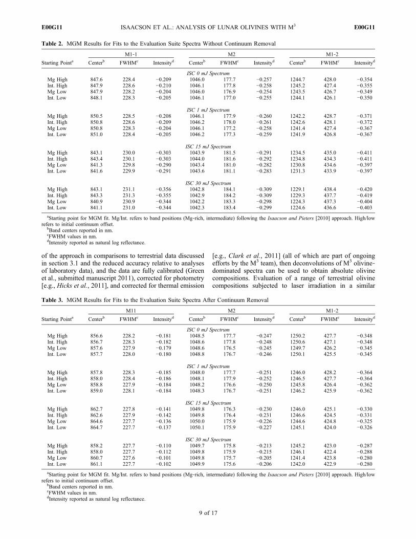
of the approach in comparisons to terrestrial data discussedin section 3.1 and the reduced accuracy relative to analysesof laboratory data), and the data are fully calibrated (Greenet al., submitted manuscript 2011), corrected for photometry[e.g., Hicks et al., 2011], and corrected for thermal emission

[e.g., Clark et al., 2011] (all of which are part of ongoingefforts by the M3 team), then deconvolutions of M3 olivine‐dominated spectra can be used to obtain absolute olivinecompositions. Evaluation of a range of terrestrial olivinecompositions subjected to laser irradiation in a similar

Table 2. MGM Results for Fits to the Evaluation Suite Spectra Without Continuum Removal

Starting PointaM1‐1 M2 M1‐2

Centerb FWHMc Intensityd Centerb FWHMc Intensityd Centerb FWHMc Intensityd

ISC 0 mJ SpectrumMg High 847.6 228.4 −0.209 1046.0 177.7 −0.257 1244.7 428.0 −0.354Int. High 847.9 228.6 −0.210 1046.1 177.8 −0.258 1245.2 427.4 −0.355Mg Low 847.9 228.2 −0.204 1046.0 176.9 −0.254 1243.5 426.7 −0.349Int. Low 848.1 228.3 −0.205 1046.1 177.0 −0.255 1244.1 426.1 −0.350



ISC 30 mJ SpectrumMg High 843.1 231.1 −0.356 1042.8 184.1 −0.309 1229.1 438.4 −0.420Int. High 843.3 231.3 −0.355 1042.9 184.2 −0.309 1229.3 437.7 −0.419Mg Low 840.9 230.9 −0.344 1042.2 183.3 −0.298 1224.3 437.3 −0.404Int. Low 841.1 231.0 −0.344 1042.3 183.4 −0.299 1224.6 436.6 −0.403aStarting point for MGM fit. Mg/Int. refers to band positions (Mg‐rich, intermediate) following the Isaacson and Pieters [2010] approach. High/low

refers to initial continuum offset.bBand centers reported in nm.cFWHM values in nm.dIntensity reported as natural log reflectance.

Table 3. MGM Results for Fits to the Evaluation Suite Spectra After Continuum Removal

Starting PointaM11 M2 M1‐2

Centerb FWHMc Intensityd Centerb FWHMc Intensityd Centerb FWHMc Intensityd




ISC 30 mJ SpectrumMg High 858.2 227.7 −0.110 1049.7 175.8 −0.213 1245.2 423.0 −0.287Int. High 858.0 227.7 −0.112 1049.8 175.9 −0.215 1246.1 422.4 −0.288Mg Low 860.7 227.6 −0.101 1049.8 175.7 −0.205 1241.4 423.8 −0.280Int. Low 861.1 227.7 −0.102 1049.9 175.6 −0.206 1242.0 422.9 −0.280aStarting point for MGM fit. Mg/Int. refers to band positions (Mg‐rich, intermediate) following the Isaacson and Pieters [2010] approach. High/low

refers to initial continuum offset.bBand centers reported in nm.cFWHM values in nm.dIntensity reported as natural log reflectance.


9 of 17

manner to the evaluation suite would be a logical area ofadditional research. Such work would enable the methodspresented here to predict absolute olivine compositionsmuch more reliably.

5.2. Application to M3 Spectra

[24] We performed continuum removal on the M3 spectrawith the same method used for the laboratory spectra. The

results of MGM deconvolutions to these spectra are reportedin the auxiliary material, with only the results of the inter-mediate starting point reported, as discussed in section 4.Example fits, to the same example M3 spectra shown inFigure 8, are shown in Figure 10. Immediately apparent isthe higher level of “noise” in the M3 spectra relative tolaboratory spectra, as evidenced by the high‐frequencyvariation in the input spectra (gray X’s). Also apparent is the

Table 4. Comparison of MGM‐Derived Band Centers for Evaluation Suite Spectra, With and Without Continuum Removal

Fit

Center Center CRa

Continuum Slopeb Continuum InterceptM1‐1 M2 M1‐2 M1‐1 M2 M1‐2

ISC 0 mJ SpectrumMg High 847.6 1046.0 1244.7 856.6 1048.5 1250.2 5.42 0.843Int. High 847.9 1046.1 1245.2 856.7 1048.6 1250.6Mg Low 847.9 1046.0 1243.5 857.6 1048.6 1249.7Int. Low 848.1 1046.0 1244.1 857.7 1048.8 1250.1




aCR, continuum removed.bContinuum slope removed from spectrum. Slope × 10−5. Units are reflectance/l, l in nm.

Figure 7. MGM‐derived band centers and relative pre-dicted compositions for the evaluation suite spectra. Theevaluation suite spectra without continuum removal (“orig-inal”) span a range of band center wavelengths and pre-dicted compositions, but all samples have the sameabsolute olivine composition (Fo #). The continuum‐removed results cluster around the same band center wave-length and relative predicted composition, demonstrating theviability of our continuum removal process.

Figure 8. Example M3 spectra collected from each regionanalyzed. These do not make up the full suite of spectra ana-lyzed but are indicative of typical olivine‐rich spectra col-lected from each region. The spectra have been truncatedat 2600 nm to enable direct comparison with laboratoryspectra.


10 of 17

reduced spectral sampling of M3 across this wavelengthregion (20 nm). These factors combine to produce noisierfits, as indicated by the RMS error line. Relative to fits to thecontinuum‐removed laboratory spectra, higher continuumoffsets were used for fits to the M3 spectra. We experi-mented with a range of offset values, and found that forthese spectra, a higher offset value allowed the individualGaussians more freedom to move and converge on theappropriate fit result. Note also the apparent errors in the fitat extreme short and especially extreme long wavelengths.This is a byproduct of the high continuum offset and the useof only one Gaussian to model the outer (extreme short andlong) wavelengths. This is inconsequential to the MGM

results for the three principal olivine absorptions. Theangularity of the Gaussians (and consequentially of thespectral fit) is a product of the reduced spectral samplingof the M3 spectra in comparison to the laboratory spectra(5 nm).[25] The reduced spectral sampling and increased noise

levels in M3 spectra relative to laboratory spectra mean thatthe compositional predictions based on MGM deconvolu-tions of the M3 spectra must be interpreted with caution.Even though we only evaluate composition in a relativesense, the relatively low spectral sampling make the MGManalyses fairly sensitive to noise, especially for olivineabsorptions. Olivine absorptions shift a maximum of ∼70 nmover the full compositional range (Fo100 to Fo0), equivalentto ∼3.5 M3 spectral channels in the maximum spectral res-olution used in this study (Green et al., submitted manu-script, 2011). Substantial errors in even a few channels dueto noise, especially if noise causes spurious features span-ning several channels, can introduce serious biases in the fitresults. Even in analyzing telescopic data of asteroids withhigher signal levels and spectral sampling, Sunshine et al.[2007] classified olivine compositions into only threebroad groups. Despite these cautions, the M3 data analyzedhere do show clear spectral variability, as discussed below,and this variability was quantified with the MGM.5.2.1. Qualitative Spectral Diversity[26] Representative examples of the spectra analyzed in

this study are illustrated with common continuum removaland scaled absorption magnitudes in Figure 9. This scalingapproach allows true spectral variability to be evaluated moreeasily, as it eliminates complicating factors such as vari-able spectral contrast, albedo, and continuum slope. WhileFigure 9a is the most useful for absolute comparisons,Figure 9b shows the individual spectra more clearly, reduc-ing clutter. Figure 9 illustrates that there are spectral dif-ferences between the suites of olivines analyzed. TheMoscoviense and Copernicus olivines are fairly similar,although the Moscoviense olivine spectrum plotted inFigure 9 exhibits a slightly broader long‐wavelength absorp-tion that the Copernicus spectrum. However, the Copernicusspectrum in this region may be biased by the sharp featurenear 1500 nm that gives the illusion of a strong but relativelynarrow long‐wavelength absorption. This sharp feature near1500 nm is in the spectral region of a filter boundary on theM3 detector (Green et al., submitted manuscript, 2011) andthus likely is not a “real” feature. The Copernicus spectraalso exhibit a fairly sharp “dip” in reflectance near ∼850 nmthat is observed consistently across the Copernicus suite andlikely is not “real.” This feature will influence the MGMdeconvolutions. The Moscoviense olivines were observed tobe more spectrally diverse than the Copernicus olivines,which are remarkably homogeneous. The Aristarchus andMarius spectra exhibit prominent differences from theCopernicus and Moscoviense olivine spectra.[27] The Aristarchus spectrum exhibits a prominent fea-

ture near 1300 nm. A feature of this relative magnitude atthis wavelength is inconsistent with pure olivine [Burns,1970; Sunshine and Pieters, 1998], although very Fe‐richolivines do tend to exhibit stronger long‐wavelength (M1‐2)absorptions [Sunshine and Pieters, 1998]. However, theAristarchus spectrum exhibits a relatively short‐wavelengthband minimum, which would be at odds with a very Fe‐rich

Figure 9. Comparison of olivine spectra. Representativeexample M3 spectra from each suite evaluated are plotted,as are example laboratory spectra (Fo90 and Fo60) and twoof the evaluation suite spectra (0 mJ and 30 mJ). The Fo60spectrum is discussed by Dyar et al. [2009]. The spectraare shown after continuum removal and normalization suchthat the band strength ranges from zero to one for all spectra,eliminating complications such as variable albedo, spectralcontrast, and slope. Spectra are shown (a) on the same axesand (b) offset for clarity.


11 of 17

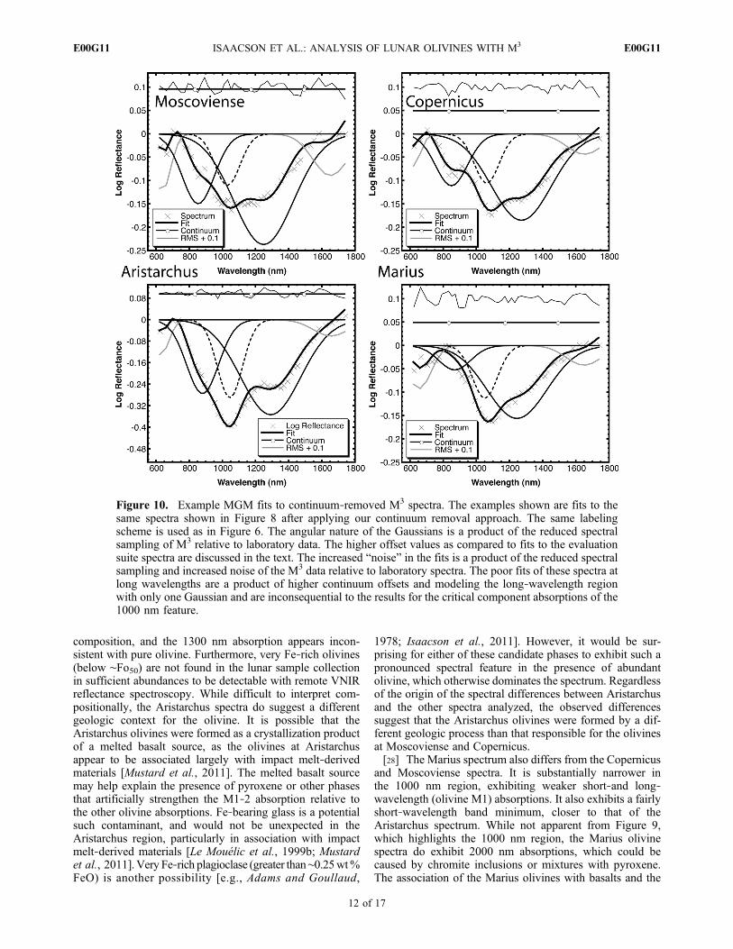
composition, and the 1300 nm absorption appears incon-sistent with pure olivine. Furthermore, very Fe‐rich olivines(below ∼Fo50) are not found in the lunar sample collectionin sufficient abundances to be detectable with remote VNIRreflectance spectroscopy. While difficult to interpret com-positionally, the Aristarchus spectra do suggest a differentgeologic context for the olivine. It is possible that theAristarchus olivines were formed as a crystallization productof a melted basalt source, as the olivines at Aristarchusappear to be associated largely with impact melt‐derivedmaterials [Mustard et al., 2011]. The melted basalt sourcemay help explain the presence of pyroxene or other phasesthat artificially strengthen the M1‐2 absorption relative tothe other olivine absorptions. Fe‐bearing glass is a potentialsuch contaminant, and would not be unexpected in theAristarchus region, particularly in association with impactmelt‐derived materials [Le Mouélic et al., 1999b; Mustardet al., 2011].Very Fe‐rich plagioclase (greater than∼0.25wt%FeO) is another possibility [e.g., Adams and Goullaud,

1978; Isaacson et al., 2011]. However, it would be sur-prising for either of these candidate phases to exhibit such apronounced spectral feature in the presence of abundantolivine, which otherwise dominates the spectrum. Regardlessof the origin of the spectral differences between Aristarchusand the other spectra analyzed, the observed differencessuggest that the Aristarchus olivines were formed by a dif-ferent geologic process than that responsible for the olivinesat Moscoviense and Copernicus.[28] The Marius spectrum also differs from the Copernicus

and Moscoviense spectra. It is substantially narrower inthe 1000 nm region, exhibiting weaker short‐and long‐wavelength (olivine M1) absorptions. It also exhibits a fairlyshort‐wavelength band minimum, closer to that of theAristarchus spectrum. While not apparent from Figure 9,which highlights the 1000 nm region, the Marius olivinespectra do exhibit 2000 nm absorptions, which could becaused by chromite inclusions or mixtures with pyroxene.The association of the Marius olivines with basalts and the

Figure 10. Example MGM fits to continuum‐removed M3 spectra. The examples shown are fits to thesame spectra shown in Figure 8 after applying our continuum removal approach. The same labelingscheme is used as in Figure 6. The angular nature of the Gaussians is a product of the reduced spectralsampling of M3 relative to laboratory data. The higher offset values as compared to fits to the evaluationsuite spectra are discussed in the text. The increased “noise” in the fits is a product of the reduced spectralsampling and increased noise of the M3 data relative to laboratory spectra. The poor fits of these spectra atlong wavelengths are a product of higher continuum offsets and modeling the long‐wavelength regionwith only one Gaussian and are inconsequential to the results for the critical component absorptions of the1000 nm feature.


12 of 17

nature of the 2 mm absorptions suggest that the Mariusolivine spectra exhibit minor contamination from pyroxene,although the pyroxene composition is uncertain. Pyroxenecontamination would also help to explain the relativelynarrow 1000 nm absorption, as well as the short‐wavelengthband minimum. The spectral variability between Marius andthe other spectra evaluated suggests a different compositionor lithological association.5.2.2. Quantitative Spectral Diversity[29] The MGM fits quantify the spectral variability illus-

trated in Figure 9. The relative predicted olivine composi-tions derived from the deconvolutions to the Moscovienseand Copernicus spectra are presented in Figure 11. Asexpected based on their overall similarity in Figure 9, theMoscoviense and Copernicus olivines are predicted to bequite similar in composition, although the spectral variabilityof the Moscoviense spectra is manifested in the larger rangein estimated relative composition (∼30 relative Fo # units).The Copernicus deconvolutions appear to be balanced bycompeting influences: the apparently strong but narrowlong‐wavelength absorption and the sharp feature near∼850 nm. The Aristarchus and Marius spectra are clearlyolivine‐rich, but the contamination from other phases pre-vents us from using MGM fits to predict the olivines’compositions, as discussed in section 5.2.3.[30] Figure 11 also illustrates the error brackets deter-

mined using the methods described above in section 3.3.2.The error brackets in effect indicate the range of resultsobtained from various fitting procedures applied to a single

Table 5. Local Continuum Slopes Removed From M3 SpectraPrior to MGM Fits

SpectrumContinuumSlopea

ContinuumOffset Tan l Shortb Tan l Longb

Mosc‐9 9.80E‐05 0.317 730 1700Mosc‐12 8.80E‐05 0.248 730 1700Mosc‐16 1.57E‐04 0.238 730 1700Mosc‐17 1.36E‐04 0.298 730 1700Mosc‐18 1.29E‐04 0.353 730 1700Mosc‐21 1.04E‐04 0.169 730 1700Mosc‐22 9.40E‐05 0.147 730 1700Mosc‐23 1.06E‐04 0.146 730 1700Mosc‐24 8.10E‐05 0.166 730 1700Mosc‐25 1.27E‐04 0.137 730 1700Cop‐1 1.40E‐04 0.113 730 1700Cop‐2 1.32E‐04 0.087 730 1700Cop‐3 1.15E‐04 0.076 730 1700Cop‐4 1.21E‐04 0.071 730 1700Cop‐5 7.50E‐05 0.105 730 1700Cop‐6 1.27E‐04 0.089 730 1700Cop‐7 1.70E‐04 0.120 730 1700Cop‐8 1.55E‐04 0.079 730 1700Cop‐9 8.90E‐05 0.051 730 1700Arist‐S1 5.30E‐05 0.032 730 1700Arist‐S2 8.20E‐05 0.077 730 1700Arsit‐S3 5.90E‐05 0.052 730 1700Marius‐1 4.10E‐05 0.089 790 1700Marius‐2 4.80E‐05 0.062 790 1700Marius‐3 4.60E‐05 0.062 790 1700

aSlope value assumes band shifts are in units of nm, and local continuumslopes are in units of reflectance/nm.

bTan stands for tangent.

Figure 11. MGM‐derived band center wavelengths and relative predicted compositions for the M3 spec-tra analyzed in this study. The large ticks on the relatlive Fo # axis denote intervals of 20 relative Fo #units. The plotted results are reported in Table S1 in the auxiliary material. There is some deviation fromthe trends developed for terrestrial olivines by Sunshine and Pieters [1998], most notably for the centralM2 absorption, but the overall agreement is reasonable. Error “range” brackets are reported for eachcomponent absorption (two‐dimensional range) and for an overall range in predicted compositions. Thecomposite error reflects the range in predicted composition when considering the ranges for each com-ponent absorption simultaneously. Error analysis is discussed more thoroughly in section 3.3.2.


13 of 17

M3 spectrum. The error brackets (and the associated com-posite error bracket) do not evaluate the effect of eachpotential source of error (e.g., reduced spectral resolution,increased noise, etc.) explicitly, but do evaluate them in thesense that all sources of error contribute to the observedranges. Future work on this subject will likely focus ondeconvolutions of laboratory spectra with reduced spectralsampling and various levels of random noise introduced inorder to quantify these effects more explicitly. Even in theideal case of MGM deconvolutions of laboratory olivinereflectance spectra, compositional predictions with thisapproach can be accurate only to within ∼5–10% (5–10 Fo #units) [Sunshine and Pieters, 1998; Isaacson and Pieters,2010]. The range predicted for the “composite error” is onthe order of 20 Fo # units (on a 0–100 scale in molar Mg/Mg+Fe *100). Thus, our reported compositions should beviewed and interpreted as approximate solutions, even in arelative sense.[31] The relative olivine compositions predicted from the

M3 spectra can be used to draw some geological inter-pretations. The Moscoviense olivines appear to be diversebut Mg‐rich relative to the other olivines evaluated here.The most Mg‐rich compositions found at Moscovienseappear consistent with the evaluation suite results, which inabsolute terms are similar to some of the most Mg‐richolivines found in Mg suite rocks with compositions near∼Fo90 [e.g., Papike et al., 1998]. While there are reasons tobe cautious in interpreting this similarity, it is suggestivethat the olivines found to be the most Mg‐rich in the regionmay be quite Mg‐rich in absolute terms as well. This maysuggest that these olivines are derived from a relativelyprimitive plutonic source, which would be consistent withthe plutonism hypothesized to have produce the unusualmafic lithologies observed elsewhere in the Moscovienseregion [Pieters et al., 2011]. Our results do not allow us toevaluate a possible genetic relationship to the olivinesstudied at Moscoviense and those identified in associationwith unusual exposures of olivine, orthopyroxene, and spinel(OOS) by Pieters et al. [2011], largely because the olivinesidentified by Pieters et al. do not exhibit sufficient spectralcontrast or purity to evaluate with our current approach.However, such a comparison would be a logical avenue forfuture work if the spectral contrast and purity issues can beovercome. The diversity of the olivine compositionsobserved at Moscoviense may indicate a long‐lived geologicprocess capable of producing a trend in olivine compositionstoward more Fe‐rich compositions as the olivine’s sourcematerial evolved. The observed diversity is distributedacross a relatively small spatial region (less than 100 km2),and a wide variation in olivine composition across a smallarea is difficult to explain petrologically. However, the largeerror bars in these analyses may help explain some of thewidespread variation (the actual compositional diversitymay be magnified by errors). Additionally, it is of coursepossible that random noise may contribute to the observedheterogeneity. However, the real spectral differences appar-ent in Figure 9 suggest that real compositional variability islargely responsible for the spread in predicted compositions.Regardless, the diverse compositions observed for theMoscoviense olivines suggest a different process than thatresponsible for the olivines at Copernicus, which are spec-trally (and thus compositionally) more homogenous.

[32] The olivines at Copernicus are found to be relativelyMg‐rich, comparable to the most Mg‐rich of the composi-tions predicted at Moscoviense. Additionally, they are morespectrally and thus compositionally homogeneous thanthose observed at Moscoviense. Their predicted composi-tions are also similar to those of the evaluation suite spectra.The consistency between all spectra analyzed for theCopernicus central peak indicates that the olivine is fairlyhomogenous in composition, which is consistent with asingle magmatic or mantle source, rather than a process inwhich a source region evolved over time producing a trendof increasing olivine Fe contents. The relatively Mg‐richcompositions argue against a volcanic origin and in favor ofa plutonic origin, as olivines in mare basalt largely (but notalways) tend to be somewhat more Fe‐rich [e.g., Papikeet al., 1976]. As the Aristarchus and Marius spectra exhibitclear contributions from absorptions not due to olivine, weelect not to model them with the MGM, as the results wouldbe biased by the other absorptions in the general 1000 nmregion where the principal olivine absorptions are found. Wemerely point out their clear spectral differences from theMoscoviense and Copernicus spectra, which alone are suf-ficient to demonstrate the different lithological associationsof the Aristarchus and Marius olivines relative to those atMoscoviense and Copernicus.5.2.3. Mixtures[33] Currently, our approach is likely to produce mean-

ingful results only for spectra in which olivine is the dom-inant phase (i.e., no other ferrous absorptions in the 1000 nmregion). This rules out compositional analyses of pyroxene‐olivine mixtures. Olivine‐plagioclase mixtures can be ana-lyzed, especially if the plagioclase is in its shocked form(maskelynite) and lacks its typical feature near 1300 nm[e.g., Bell and Mao, 1973; Adams and Goullaud, 1978;Pieters, 1996]. Crystalline, Fe‐bearing plagioclase doesexhibit absorptions near 1300 nm, and if such absorptionfeatures were detectible in the olivine‐plagioclase mixturespectrum, that spectrum could not be analyzed with ourpresent approach. However, the plagioclase absorption fea-ture does tend to get masked by other mafic absorptionssuch as those of olivine and pyroxene [e.g., Isaacson et al.,2011], meaning that olivine‐plagioclase mixtures generallycan be analyzed with our approach except in rare caseswhere the plagioclase absorption feature persists.[34] In principle, our approach could be applied to spectra

of mixtures such as olivine‐pyroxene. The potential pro-blems associated with extending the approach to mixturespectra lie in determining the properties of the olivineabsorptions in the presence of additional absorptions near1000 nm, as discussed above in the context of the Mariusolivine spectra. The MGM seeks a mathematically opti-mized solution, without regard for whether or not the fit isphysically reasonable (consistent with the mineralogy of thematerial represented by the input spectrum). Each Gaussianis based on three model parameters (position, strength, andwidth), so the presence of additional absorption featuressubstantially increases the number of free parameters in themodel, and reduces the likelihood of obtaining a unique andphysically reasonable fit. McFadden and Cline [2005] usedthe MGM to model laboratory reflectance spectra of Martianmeteorites, including several containing mixtures of olivineand pyroxene. While they were able to produce reasonable


14 of 17

fits in some cases, they were unable to produce acceptablefits for several other such mixtures, even in analyzingoptimal quality laboratory spectra. The increased noise leveland decreased spectral resolution of M3 relative to labora-tory spectra have been discussed above, and combine tomake obtaining acceptable results for pyroxene/olivinemixtures extremely challenging with the current approach.However, if a method to constrain the model parametersappropriately and allow the olivine absorptions to bedeconvolved properly were available, our approach couldcertainly be used to estimate the composition of the olivine.For example, the 2000 nm pyroxene absorption featurecould be used to help constrain the Gaussian(s) used tomodel the pyroxene 1000 nm absorption feature, as theproperties of the pyroxene absorption features are related[e.g., Adams, 1974; Hazen et al., 1978; Cloutis et al., 1986;Klima, 2008]. In the case of lunar olivine, however, thisapproach would in turn be complicated by the presence ofthe chromite absorptions near 2000 nm.

6. Conclusions

[35] Our analyses of olivines using Chandrayaan‐1 MoonMineralogy Mapper (M3) spectra have produced intriguingresults. Suites of olivine reflectance spectra collected fromdiverse regions on the lunar surface exhibit spectral vari-ability through visual comparisons. The MGM was used toquantify these observations for the olivine‐dominatedspectra. Olivine from the Copernicus central peak was foundto be fairly homogenous and, broadly speaking, composi-tionally similar to olivines from Moscoviense, though theMoscoviense olivines were found to be slightly morespectrally and thus compositionally diverse. While thecautions presented here must be considered carefully, themethods presented in this paper can be used to make generalpredictions of absolute olivine composition (Fe/Mg content)with remotely sensed VNIR reflectance spectra. While theerror bars in our results are substantial given the numerousissues discussed here, our results suggest the detection ofMg‐rich olivine at Moscoviense and Copernicus with M3

spectra. Olivines from the Aristarchus crater were found tobe exhibit a strong long‐wavelength absorption, likely dueto contamination by a presently unknown phase. The originof this strong long‐wavelength absorption is presentlyunclear, but it does suggest a compositional difference or atleast a different lithological association than exhibited by theMoscoviense and Copernicus olivines. Olivines at Mariuswere found to exhibit contamination, likely by pyroxene,which again hints at a different lithological association thanexhibited by the olivines at Copernicus and Moscoviense.[36] The present study has demonstrated a systematic

approach for addressing variable continuum slopes commonto remotely sensed spectra of planetary surfaces, and dis-cussed some of the strengths and weaknesses of this sim-plified but easily repeatable and consistent approach. Usinga suite of laboratory spectra, we have demonstrated that ourtangential continuum removal process is able to treat theeffects of variable continuum slopes in a consistent manner.This is a vital step, as lack of such a treatment would lead toderived band positions (and thus predicted compositions)that are strongly biased by continuum slopes. The reducedspectral sampling and lower signal‐to‐noise ratio of the M3

spectra relative to typical laboratory spectra affect theaccuracy of compositional predictions. We have quantifiedthe likely range in a predicted composition, but have nottreated sources of error explicitly beyond their contributionto a bulk overall “error” in our relative compositional pre-dictions. Future work on this topic will involve expandingthe survey to analyze olivines from more regions on thelunar surface.

[37] Acknowledgments. The efforts of the entire M3 engineering,operations, and science teams are gratefully acknowledged. M3 sciencevalidation is supported through NASA contract NNM05AB26C. M3 issupported as a NASA Discovery Program mission of opportunity. TheM3 team is grateful to ISRO for the opportunity to fly as a guest instrumenton Chandrayaan‐1. Partial funding for this analysis has also been providedthrough the NASA LSI at Brown University under contract NNA09DB34A.Careful reviews by Brett Denevi and an anonymous reviewer haveimproved this manuscript substantially. The views, opinions, and/or find-ings contained in this paper are those of the authors and should not beinterpreted as representing the official views, either expressed or implied,of the Defense Advanced Research Projects Agency or the Department ofDefense.

ReferencesAdams, J. B. (1974), Visible and near‐infrared diffuse reflectance spectraof pyroxenes as applied to remote sensing of solid objects in the solarsy s t em , J . Geophy s . Res . , 79 , 4829–4836 , do i : 10 . 1029 /JB079i032p04829.

Adams, J. B., and L. H. Goullaud (1978), Plagioclase feldspars: Visible andnear infrared diffuse reflectance spectra as applied to remote sensing,Proc. Lunar Planet Sci., 9, 2901–2909.

Andersson, L. E., and E. A. Whitaker (1982), NASA Catalogue of LunarNomenclature, NASA Ref. Publ., 1097.

Aronson, J. R., L. H. Bellotti, S. W. Eckroad, R. K. McConnell, and P. C.Von Thüna (1970), Infrared spectra and radiative thermal conductivity ofminerals at high temperatures, J. Geophys. Res., 75(17), 3443–3456,doi:10.1029/JB075i017p03443.

Basaltic Volcanism Study Project (BVSP) (1981), Basaltic Volcanism onthe Terrestrial Planets, Pergamon, New York.

Bell, P. M., and H. K. Mao (1973), Optical and chemical analysis of iron inLuna 20 plagioclase, Geochim. Cosmochim. Acta, 37, 755–759,doi:10.1016/0016-7037(73)90172-5.

Besse, S., J. M. Sunshine, M. I. Staid, N. E. Petro, J. W. Boardman, R. O.Green, J. W. Head, P. J. Isaacson, J. F. Mustard, and C. M. Pieters(2011), Compositional variability of the Marius Hills Volcanic Complexfrom the Moon Mineralogy Mapper (M3), J. Geophys. Res., doi:10.1029/2010JE003725, in press.

Boardman, J. W., C. M. Pieters, R. O. Green, S. Lundeen, P. Varansi,J. Nettles, N. E. Petro, P. J. Isaacson, S. Besse, and L. A. Taylor(2011), Measuring moonlight: An overview of the spatial properties,lunar coverage, selenolocation and related level 1B products of the MoonMineralogy Mapper, J. Geophys. Res., doi:10.1029/2010JE003730,in press.

Burns, R. G. (1970), Crystal field spectra and evidence of cation ordering inolivine minerals, Am. Mineral., 55, 1608–1632.

Burns, R. G. (1974), The polarized spectra of iron in silicates: Olivine. Adiscussion of neglected contributions from Fe2+ ions in M(1) sites, Am.Mineral., 59, 625–629.

Burns, R. G. (1993), Mineralogical Applications of Crystal Field Theory,2nd ed., 551 pp., Cambridge Univ. Press, New York, doi:10.1017/CBO9780511524899.

Burns, R. G., F. E. Huggins, and R. M. Abu‐Eid (1972), Polarized absorp-tion spectra of single crystals of lunar pyroxenes and olivines, Moon, 4,93–102, doi:10.1007/BF00562917.

Chevrel, S. D., P. C. Pinet, Y. Daydou, S. Le Mouélic, Y. Langevin,F. Costard, and S. Erard (2009), The Aristarchus Plateau on the Moon:Mineralogical and structural study from integrated Clementine UV VisNIR spectral data, Icarus, 199, 9–24, doi:10.1016/j.icarus.2008.08.005.

Clark, R. N. (1999), Spectroscopy of rocks and minerals, and principles ofspectroscopy, in Manual of Remote Sensing, vol. 3, Remote Sensingfor the Earth Sciences, edited by A. N. Rencz, pp. 3–58, John Wiley,New York.

Clark, R. N., and T. L. Roush (1984), Reflectance spectroscopy: Quanti-tative analysis techniques for remote sensing applications, J. Geophys.Res., 89, 6329–6340, doi:10.1029/JB089iB07p06329.


15 of 17

Clark, R. N., C. M. Pieters, R. O. Green, J. W. Boardman, and N. E. Petro(2011), Thermal removal from near‐infrared imaging spectroscopy dataof the Moon, J. Geophys. Res., doi:10.1029/2010JE003751, in press.

Cloutis, E. A., M. J. Gaffey, T. L. Jackowski, and K. L. Reed (1986),Calibrations of phase abundance, composition, and particle size distributionfor olivine‐orthopyroxene mixtures from reflectance spectra, J. Geophys.Res., 91, 11,641–11,653, doi:10.1029/JB091iB11p11641.

Cloutis, E. A., J. M. Sunshine, and R. V. Morris (2004), Spectral reflectance‐compositional properties of spinels and chromites: Implications forplanetary remote sensing and geothermometry, Meteorit. Planet. Sci.,39, 545–565, doi:10.1111/j.1945-5100.2004.tb00918.x.

Dyar, M. D., et al. (2009), Spectroscopic characteristics of synthetic olivine:An integrated multi‐wavelength and multi‐technique approach, Am.Mineral., 94(7), 883–898, doi:10.2138/am.2009.3115.

Hapke, B. (2001), Space weathering from Mercury to the asteroid belt,J. Geophys. Res., 106, 10,039–10,073, doi:10.1029/2000JE001338.

Hazen, R. M., P. M. Bell, and H. K. Mao (1978), Effects of compositionalvariation on absorption spectra of lunar pyroxenes, Proc. Lunar PlanetSci., 9, 2919–2934.

Hicks, M. D., B. J. Buratti, J. Nettles, M. Staid, J. Sunshine, C. M. Pieters,S. Besse, and J. W. Boardman (2011), A photometric function for analysisof lunar images in the visual and infrared based on Moon MineralogyMapper observations, J. Geophys. Res., doi:10.1029/2010JE003733, inpress.

Hiroi, T., and S. Sasaki (2001), Importance of space weathering simulationproducts in compositional modeling of asteroids: 349 Dembowska and446 Aeternitas as examples, Meteorit. Planet. Sci., 36, 1587–1596,doi:10.1111/j.1945-5100.2001.tb01850.x.

Isaacson, P. J., and C. M. Pieters (2010), Deconvolution of lunar olivinereflectance spectra: Implications for remote compositional assessment,Icarus, 210(1), 8–13, doi:10.1016/j.icarus.2010.06.004.

Isaacson, P. J., A. Basu Sarbadhikari, C. M. Pieters, R. L. Klima, T. Hiroi,Y. Liu, and L. A. Taylor (2011), The lunar rock and mineral character-ization consortium: Deconstruction and integrated mineralogical, petro-logic, and spectroscopic analyses of mare basalts, Meteorit. Planet.Sci., 46, 228–251, doi:10.1111/j.1945-5100.2010.01148.x.

Kanner, L. C., J. F. Mustard, and A. Gendrin (2007), Assessing the limits ofthe Modified Gaussian Model for remote spectroscopic studies of pyrox-enes on Mars, Icarus, 187, 442–456, doi:10.1016/j.icarus.2006.10.025.

King, T. V. V., and W. I. Ridley (1987), Relation of the spectroscopicreflectance of olivine to mineral chemistry and some remote sensing im-plications, J. Geophys. Res., 92, 11,457–11,469, doi:10.1029/JB092iB11p11457.

Klima, R. L. (2008), Integrated spectroscopy of synthetic Mg‐Fe‐Capyroxenes, Ph.D. thesis, 281 pp., Brown Univ., Providence, R. I.

Le Mouélic, S. (2001), The olivine at the lunar crater Copernicus as seen byClementine NIR data, Planet. Space Sci., 49, 65–70, doi:10.1016/S0032-0633(00)00091-X.

Le Mouélic, S., Y. Langevin, and S. Erard (1999a), The distribution ofolivine in the crater Aristarchus inferred from Clementine NIR data,Geophys. Res. Lett., 26, 1195–1198, doi:10.1029/1999GL900180.

Le Mouélic, S., Y. Langevin, and S. Erard (1999b), A new data reductionapproach for the Clementine NIR data set: Application to Aristillus,Aristarchus and Kepler, J. Geophys. Res., 104, 3833–3843, doi:10.1029/1998JE900035.

Lucey, P. G. (1998), Model near‐infrared optical constants of olivineand pyroxene as a function of iron content, J. Geophys. Res., 103,1703–1713, doi:10.1029/97JE03145.

Lucey, P. G., B. R. Hawke, and K. Horton (1991), The distribution ofolivine in the Crater Copernicus, Geophys. Res. Lett., 18(11), 2133–2136,doi:10.1029/91GL02538.

McFadden, L. A., and T. P. Cline (2005), Spectral reflectance of Martianmeteorites: Spectral signatures as a template for locating source regionon Mars, Meteorit. Planet. Sci., 40, 151–172, doi:10.1111/j.1945-5100.2005.tb00372.x.

Mustard, J. F., et al. (2011), Compositional diversity and geologic insightsof the Aristarchus crater fromMoonMineralogyMapper data, J. Geophys.Res., doi:10.1029/2010JE003726, in press.

Noble, S. K., C. M. Pieters, L. A. Taylor, R. V. Morris, C. C. Allen, D. S.McKay, and L. P. Keller (2001), The optical properties of the finest frac-tion of lunar soil: Implications for space weathering, Meteorit. Planet.Sci., 36, 31–42, doi:10.1111/j.1945-5100.2001.tb01808.x.

Noble, S. K., L. P. Keller, and C. M. Pieters (2005), Evidence of spaceweathering in regolith breccias I: Lunar regolith breccias, Meteorit.Planet. Sci., 40, 397–408, doi:10.1111/j.1945-5100.2005.tb00390.x.

Noble, S. K., C. M. Pieters, and L. P. Keller (2007), An experimentalapproach to understanding the optical effects of space weathering, Icarus,192(2), 629–642, doi:10.1016/j.icarus.2007.07.021.

Ohtake, M., et al. (2009), The global distribution of pure anorthosite on theMoon, Nature, 461(7261), 236–240, doi:10.1038/nature08317.

Papike, J. J., F. N. Hodges, A. E. Bence, M. Cameron, and J. M. Rhodes(1976), Mare basalts: Crystal chemistry, mineralogy, and petrology,Rev . Geophy s . Space Phy s . , 14 , 4 75–540 , do i : 10 . 1029 /RG014i004p00475.

Papike, J. J., G. Ryder, and C. K. Shearer (1998), Lunar samples, inPlanetary Materials, edited by J. J. Papike, pp. 5‐1–5‐234, Mineral.Soc. of Am., Washington, D. C.

Pieters, C. M. (1982), Copernicus crater central peak: Lunar mountain ofunique composition, Science, 215, 59–61, doi:10.1126/science.215.4528.59.

Pieters, C. M. (1986), Composition of the lunar highland crust from near‐infrared spectroscopy, Rev. Geophys. Space Phys., 24(3), 557–578,doi:10.1029/RG024i003p00557.

Pieters, C. M. (1996), Plagioclase and maskelynite diagnostic features,Lunar Planet. Sci. [CD‐ROM], 27, 1031.

Pieters, C. M. (1999), The moon as a spectral calibration standard enabledby lunar samples: The Clementine example, paper presented at Workshopon New Views of the Moon II: Understanding the Moon Through theIntegration of Diverse Datasets, Lunar and Planet. Inst., Flagstaff, Ariz.

Pieters, C. M., and D. E. Wilhelms (1985), Origin of olivine at Copernicus,Proc. Lunar Planet. Sci., 15, 415–420.

Pieters, C. M., L. A. Taylor, S. K. Noble, L. P. Keller, B. Hapke, R. V.Morris,C. C. Allen, D. S. McKay, and S. Wentworth (2000), Space weathering onairless bodies: Resolving a mystery with lunar samples, Meteorit. Planet.Sci., 35, 1101–1107, doi:10.1111/j.1945-5100.2000.tb01496.x.

Pieters, C. M., et al. (2009), The Moon Mineralogy Mapper (M3) onChandrayaan‐1, Curr. Sci., 96(4), 500–505.

Pieters, C. M., et al. (2011), Mg‐spinel lithology: A new rock‐type on thelunar farside, J. Geophys. Res., doi:10.1029/2010JE003727, in press.

Sasaki, S., T. Hiroi, K. Nakamura, Y. Hamabe, E. Kurahashi, andM. Yamada (2002), Simulation of space weathering by nanosecond pulselaser heating: Dependence on mineral composition, weathering trend ofasteroids and discovery of nanophase iron particles, Adv. Space Res.,29(5), 783–788, doi:10.1016/S0273-1177(02)00012-1.

Sasaki, S., E. Kurahashi, C. Yamanaka, and K. Nakamura (2003), Labora-tory simulation of space weathering: Changes of optical properties andTEM/ESR confirmation of nanophase metallic iron, Adv. Space Res.,31(12), 2537–2542, doi:10.1016/S0273-1177(03)00575-1.

Singer, R. B., and T. L. Roush (1985), Effects of temperature on remotelysensed mineral absorption features, J. Geophys. Res., 90, 12,434–12,444,doi:10.1029/JB090iB14p12434.

Sunshine, J. M., and C. M. Pieters (1998), Determining the compositionof olivine from reflectance spectroscopy, J. Geophys. Res., 103,13,675–13,688, doi:10.1029/98JE01217.

Sunshine, J. M., C. M. Pieters, and S. F. Pratt (1990), Deconvolution ofmineral absorption bands: An improved approach, J. Geophys. Res.,95, 6955–6966, doi:10.1029/JB095iB05p06955.

Sunshine, J. M., S. J. Bus, C. M. Corrigan, T. J. McCoy, and T. H. Burbine(2007), Olivine‐dominated asteroids and meteorites: Distinguishingnebular and igneous histories, Meteorit. Planet. Sci., 42(2), 155–170,doi:10.1111/j.1945-5100.2007.tb00224.x.

Taylor, L. A., C. M. Pieters, L. P. Keller, R. V. Morris, and D. S. McKay(2001), Lunar mare soils: Space weathering and the major effects ofsurface‐correlated nanophase Fe, J. Geophys. Res., 106, 27,985–27,999,doi:10.1029/2000JE001402.

Taylor, L. A., C. Pieters, A. Patchen, D.‐H. S. Taylor, R. V. Morris,L. P. Keller, and D. S. McKay (2010), Mineralogical and chemical char-acterization of lunar highland soils: Insights into the space weathering ofsoils on airless bodies, J. Geophys. Res., 115, E02002, doi:10.1029/2009JE003427.

Yamada, M., S. Sasaki, H. Nagahara, A. Fujiwara, S. Hasegawa, H. Yano,T. Hiroi, H. Ohashi, and H. Otake (1999), Simulation of space weather-ing of planet‐forming materials: Nanosecond pulse laser irradiation andproton implantation on olivine and pyroxene samples, Earth PlanetsSpace, 51, 1255–1265.

Yamamoto, S., et al. (2010), Possible mantle origin of olivine around lunarimpact basins detected by SELENE, Nat. Geosci., 3, 533–536,doi:10.1038/ngeo897.

S. Besse and J. M. Sunshine, Department of Astronomy, University ofMaryland, College Park, MD 20742‐2421, USA.R. N. Clark, U.S. Geological Survey, MS964, Box 25046, Federal

Center, Denver, CO 80225, USA.J. W. Head, P. J. Isaacson, J. F. Mustard, and C. M. Pieters, Department

of Geological Sciences, Brown University, Box 1846, Providence, RI02912, USA. ([email protected])


16 of 17

R. L. Klima, Johns Hopkins University Applied Physics Laboratory,11100 Johns Hopkins Rd., Laurel, MD 20732‐0000, USA.N. E. Petro, NASA Goddard Space Flight Center, Code 698, Greenbelt,

MD 20771, USA.M. I. Staid, Planetary Science Institute, 1700 E. Fort Lowell, Ste. 106,

Tucson, AZ 85719, USA.

L. A. Taylor and K. G. Thaisen, Planetary Geosciences Institute,Department of Earth and Planetary Sciences, University of Tennessee,1412 Circle Dr., Knoxville, TN 37996‐1410, USA.S. Tompkins, Defense Advanced Research Projects Agency, 3701 N.

Fairfax Dr., Arlington, VA 22203‐1714, USA.


17 of 17

Documents

Remote compositional analysis of lunar olivine rich ...sbesse/REPRINTS/Isaacson_M3olivine_2011.pdf · Remote compositional analysis of lunar olivine‐rich lithologies with Moon Mineralogy