Embed Size (px)
Citation preview

RELIABLE FRONTAL CORTEX ACTIVITY FOR AN ORAL STROOP TASK
USING FUNCTIONAL NEAR-INFRARED SPECTROSCOPY
By
MATTHEW ALLEN CLOUD
Presented to the Faculty of the Graduate School of
The University of Texas at Arlington in Partial Fulfillment
of the Requirements
for the Degree of
MASTER OF SCIENCE IN BIOMEDICAL ENGINEERING
THE UNIVERSITY OF TEXAS AT ARLINGTON
December 2013

ii
Copyright © by Matthew Allen Cloud 2013
All Rights Reserved

iii
Acknowledgements
Thank you Lord, for providing me with an opportunity to use the gifts you have given me to help
others. I thank You for blessing me with a loving and supportive wife, Nicole, our children, Caitlin,
Marcella, Volker, Dylan, Bridgette and Madeline, and my parents Nan and Wesley Cloud who have given
me unfailing support to focus and follow upon those gifts through this ordeal. To them and our extended
family and friends I can never thank you enough. Dr. Hanli Liu, thank you for guiding me through my
academic career at the University of Texas at Arlington, welcoming me into your lab, as you do so many
students each year, financial support, and giving me great insight into how to use the talents given to me.
Dr. George Alexandrakis, thank you not only for your tutelage of optical imaging, but also your ability to
see with clarity to the heart of my broad ideas. Dr. Li Zeng, thank you for arriving into my life at this
pivotal moment and helping place all the pieces together. To the staff at Pate Rehabilitation Endeavors,
particularly, Dr. Patrick Plenger, Jana Downum, Dr. Kathryn Oden, and Dr. Mary Ellen Hayden Irving,
thank you not only for providing me with the data to perform this analysis and granting me financial
support, but also guidance in the neuropsychological underpinnings of the work. The passion with which
each of you helps others is inspiring. I thank the members of Dr. Hanli Liu’s laboratory, specifically Dr.
Fenghua Tian, Dr. Vikrant Sharma, Sabin Khadka, Venki Kavuri, Lin Li, Amarnath Yennu, and Peter
Leboulluec for providing me with practical help, lofty ideological goals, imaginative troubleshooting, and
most of all their friendship. Finally, I pray that this thesis will help guide health care practitioners in their
use of functional brain imaging and improve the care of their patients.
November 18, 2013
iv
Abstract
RELIABLE FRONTAL CORTEX ACTIVITY FOR AN ORAL STROOP TASK
USING FUNCTIONAL NEAR-INFRARED SPECTROSCOPY
Matthew Cloud, MS
The University of Texas at Arlington, 2013
Supervising Professor: Hanli Liu
Analysis tools such as HomER and NIRS-SPM for functional Near-Infrared systems are
commercially or freely available; however, they are difficult for clinicians to use as an assessment tool.
One barrier to their use is the reliability of a given functional test. Intraclass correlation coefficients (ICC)
provide a measure of group and individual reliability. NIRS-SPM was extended with ICC to assess a two
part modified Stroop task. The protocol was repeated once every two weeks over a period of one month.
Changes in neural activity attributed to inhibition of distraction, show significant covariance to the protocol
with moderate to strong reliability for the group, and moderate reliability for individuals in the medial and
left frontopolar and dorsolateral cortex. In addition, as the inhibitory response increases, neural activity
shows a decrease in these same areas. This methodology could be extended to aid clinicians for group and
individual patient comparisons.

v
Table of Contents
Acknowledgements ......................................................................................................................... iii
Abstract ........................................................................................................................................... iv
List of Illustrations ........................................................................................................................ viii
List of Tables ................................................................................................................................... x
Chapter 1 Introduction ..................................................................................................................... 1
1.1 Frontal Cortex Anatomy ........................................................................................................ 2
1.2 Executive Function ................................................................................................................ 3
1.3 Stroop Test ............................................................................................................................. 3
1.4 Principles of Functional Near-Infrared Spectroscopy ............................................................ 3
1.5 Stroop Test and Functional Imaging ...................................................................................... 4
Chapter 2 Stroop Test Reliability ..................................................................................................... 7
2.1 Aims ....................................................................................................................................... 7
2.2 Materials ................................................................................................................................ 7
2.2.1 Subjects .......................................................................................................................... 7
2.2.2 Instruments ..................................................................................................................... 8
2.3 Methods ................................................................................................................................. 9
2.3.1 Experimental Design ...................................................................................................... 9
2.3.2 Experimental Protocol ...................................................................................................10
2.3.3 Behavioral Data .............................................................................................................11

vi
2.3.4 Task vs. Oxygenated Hemoglobin Covariance (NIRS-SPM) ........................................11
2.3.5 Intraclass Correlation Coefficients ................................................................................13
Chapter 3 Behavioral Analysis ........................................................................................................16
3.1 Simple and Interference Tasks ..............................................................................................16
3.2 Inhibitory Response ..............................................................................................................19
Chapter 4 NIRS-SPM Imaging .......................................................................................................21
4.1 NIRS-SPM Individual Analysis ............................................................................................21
4.1.1 Simple Task ...................................................................................................................22
4.1.2 Interference Task ...........................................................................................................24
4.1.3 Inhibition of Distraction ................................................................................................26
4.2 NIRS-SPM Group Analysis ..................................................................................................28
4.2.1 Simple Task ...................................................................................................................28
4.2.2 Interference Task ...........................................................................................................29
4.2.3 Inhibition of Distraction ................................................................................................30
4.2.4 All Sessions Group Images ............................................................................................31
Chapter 5 Reliability .......................................................................................................................32
5.1 Simple Task Reliability ........................................................................................................33
5.2 Interference Task Reliability .................................................................................................34
5.3 Inhibition of Distraction Reliability ......................................................................................36
Chapter 6 Correlation of HbO to Task Performance .......................................................................38
6.1 Simple Task HbO and Performance Correlation ..................................................................39
6.2 Interference Task HbO and Performance Correlation...........................................................40

vii
6.3 HbO and Performance Correlation for the Inhibitory Response ...........................................41
Chapter 7 Discussion .......................................................................................................................44
7.1 Simple Task ..........................................................................................................................44
7.2 Interference Task ..................................................................................................................45
7.3 Inhibition of Distraction ........................................................................................................45
7.4 Conclusion ............................................................................................................................46
Appendix A Brodmann Anatomical References to Channels .........................................................47
Appendix B Group NIRS-SPM t-maps ...........................................................................................53
Appendix C Kolmogorov-Smirnov One Sample Tests ...................................................................62
Appendix D Channel-wise Statistics .............................................................................................102
References .....................................................................................................................................108
Biographical Information ..............................................................................................................111

viii
List of Illustrations
Figure 1.2 Frontal Cortex ................................................................................................................. 2
Figure 2.1 Channels ......................................................................................................................... 8
Figure 2.2 Analysis Methods Overview ........................................................................................... 9
Figure 2.3 Experimental Design ......................................................................................................10
Figure 2.4 Protocol ..........................................................................................................................11
Figure 2.5 NIRS-SPM Analysis ......................................................................................................12
Figure 2.6 Reliability Analysis ........................................................................................................14
Figure 3.1 Percent Correct By Task and Session with Standard Error ............................................17
Figure 3.2 Simple Task Variances ..................................................................................................18
Figure 3.3 Interference Task Variances ..........................................................................................19
Figure 3.4 Change in %Correct Due to Inhibitory Response ..........................................................20
Figure 4.1 Subject 1 Task A by Session, α=0.05, Euler Characteristics .........................................22
Figure 4.2 Simple Task Subjects 1-7 t-map Images, α=0.05, Euler Characteristics .......................23
Figure 4.3 Simple Task Subjects 8-14 t-map Images, α=0.05, Euler Characteristics .....................24
Figure 4.4 Interference Task Subjects 1-7 t-map Images, α=0.05, Euler Characteristics................25
Figure 4.5 Interference Task Subjects 8-14 t-map Images, α=0.05, Euler Characteristics..............26
Figure 4.6 Inhibition of Distraction Subjects 1-7 t-map Images, α=0.05, Euler Characteristics .....27
Figure 4.7 Inhibition of Distraction Subjects 8-14 t-map Images, α=0.05, Euler Characteristics ...28
Figure 4.8 Group Simple Task t-maps Images, α=0.05, No Correction ..........................................29
Figure 4.9 Group Interference Task t-maps Images, α=0.05, No Correction ..................................29
Figure 4.10 Group Interference Task t-maps Images, α=0.05, Euler Characteristics ......................30
Figure 4.11 Group Inhibition of Distraction t-map Images, α=0.05, No Correction .......................30
Figure 4.12 Group t-maps Images for All Sessions by Task and Correction Method (n=40) .........31

ix
Figure 5.1 Reliable and Significant Channel Locations for the Simple Task ..................................34
Figure 5.2 Reliable and Significant Channel Locations for the Interference Task ..........................36
Figure 5.3 Reliable and Significant Channel Locations for Inhibition of Distraction .....................37
Figure 6.1 Simple Task %Success Correlation to HbO by Session ................................................40
Figure 6.2 Interference Task %Success Correlation to HbO by Session.........................................41
Figure 6.3 Inhibition of Distraction Correlation to HbO Difference by Session .............................43
Figure 7.1 Group t-maps for All Sessions by Task with Reliability Overlay ..................................44

x
List of Tables
Table 5.1 Reliable and Significant Channels for the Simple Task ..................................................33
Table 5.3 Reliable and Significant Channels for the Interference Task ..........................................35
Table 5.4 Reliable and Significant Channels for Inhibition of Distraction .....................................36
Table 6.1 HbO to Task Performance for All Sessions ....................................................................38
Table 6.2 Simple Task %Success correlation to HbO .....................................................................39
Table 6.3 Interference Task Correlation to %Success .....................................................................41
Table 6.4 Inhibition of Distraction Correlation to HbO Difference ................................................42

1
Chapter 1
Introduction
Over 1.7 million United States citizens receive a traumatic brain injury every year.1 Traumatic
brain injury (TBI) and stroke combine as acquired brain injury (ABI) to be the number one cause of death
and disability worldwide. TBI characteristics depend upon the specific physics of the injury such as a fall
or vehicular accident and involve a coup (anterior) and contrecoup (posterior) injury. The frontal cortex is
particularly vulnerable to TBI.2 Cognitive and behavioral impairment associated with frontal injury results
in poor recovery following injury. To maximize patient treatment it is imperative to quantify patient
capabilities and impairment. Traditionally, neuropsychologists use structural neuroradiologic imaging
combined with cognitive and behavioral assessment to determine impairments associated with frontal
cerebral injury related to TBI.3 A patient’s ability to focus on therapy tasks can change the type of therapy
and length of therapy needed for a specific patient. However, insurance companies in Texas are citing the
lack of research on the recovery of patients undergoing therapy as a basis to limit payment for patients to
six weeks. Therefore rehabilitation clinics are looking for ways to quantify the resulting improvements of
therapy. The Stroop test is used as a measure in neuropsychology to determine a patient’s ability to inhibit
distraction, i.e. focus. This test’s behavioral analysis based upon error rates undergoes habituation and may
not lend itself as a sole measure for retesting during therapy. Functional Near-infrared Spectroscopy
(fNIRS) allows a clinician to be able to infer the changes in neuronal activity of the brain cortex every tenth
of a second. This study uses fNIRS to study healthy controls taken by clinicians at a post-acute
rehabilitation clinic to determine the role of the frontal cortex to inhibit distraction and thereby determine a
normal subject’s ability to inhibit distraction and compare in the future to patient images to guide therapy
conditions. By understanding the role of the frontal cortex in the Stroop task an extended study could be
developed to help guide the length of therapy needed for patient recovery in regards to inhibiting

2
distraction. However, before comparisons can be to patients a measure of reliability within the healthy
population is first required.
1.1 Frontal Cortex Anatomy
The frontal cortex (Fig 1.1) is comprised of the prefrontal cortex and the frontopolar cortex. The
frontopolar cortex (FPC) can be broken down into a left, medial and right cortex. The prefrontal cortex is
comprised in the superior region bilaterally by the dorsolateral prefrontal cortex (DLPFC), inferior bilateral
regions of the prefrontal cortex are referred to as orbitofrontal cortex (OFC) and the lateral regions are the
ventrolateral prefrontal cortex (VLPFC). The left lateral position of the ventrolateral and dorsolateral
cortices contain Broca’s area which is the cortical area used for speech generation and recognition. While
not the focus of this study to probe geometry used for this study extends to into the motor and temporal
cortices. Superior and posterior to Broca’s area is the premotor and motor cortices associated with
movement of the mouth. Posterior to Broca’s area is the auditory regions which are in the temporal cortex.
Parallel to these speech structures on the right side there are mirrored areas of activity which may also be
associated with speech and mouth movement.
Figure 1.1 Frontal Cortex

3
The frontal cortex has many neural network pathways, but of specific concern to this study is the
pathway of the Anterior Cingulate Cortex (ACC) to DLPFC. The ACC is located in the limbic region of
the brain and associated with executive functions as well as pain. The DLPFC and FPC override the
primary brain response within the ACC.
1.2 Executive Function
Executive function is one’s ability to control other tasks. The areas of the brain considered to be
the most influential on executive function are the DLPFC and FPC. These cortices also called Brodmann
Areas 9 and 10 respectively have been determined in early lesion studies and recognized in newer
functional imaging techniques to be attributed with the ability to inhibit distraction.
1.3 Stroop Test
The Stroop test is used as an assessment to determine one’s ability to inhibit neuronal activity. In
particular, it monitors the ability to inhibit distraction and focus on naming the color presented to them,
regardless of how it is presented. The test may consist of two or many parts. It can have one or two simple
tasks as comparators to a task with a distraction. The simple task is a color block and the subject says the
color or selects the matching color with a finger press. A secondary simple task may be a list of words
written in black which the subject reads. The distracted task may be a combination of congruent or
incongruent tasks or they may be separated into different tasks. A congruent task means the color of the
word matches the font color and the subject could either read the word or say the color and they would still
be correct. The incongruent task is one where the text of the word and font color does not match. The
subject is to say only the color. If they were instead to read the text they would have the answer incorrect.
Difficulty of the task is increased by mixing congruent and incongruent presentations within the same task.
While the differences in groups for each task may be compared, the differences between the distracted task
and the simple task are normally compared for a given patient to a healthy population. Specifically the
difference in the response delay or the success rate per task is compared against different populations.
1.4 Principles of Functional Near-Infrared Spectroscopy
Functional Near-Infrared Spectroscopy is primarily used to determine the changes in
concentrations of Oxygenated Hemoglobin (HbO) and Deoxygenated Hemoglobin (Hb). These two

4
concentrations when added together determine the Total Hemoglobin (HbT) concentration change for a
given area over a specific period of time. To determine the concentrations, two wavelengths of light within
the range of 700-900 nm of what is called the near-infrared range are used to calculate the change in optical
density. This range is within the optical window (700-1000) of biological tissue meaning most tissue is
transparent to light of these wavelengths. However HbO and Hb absorb light within this range with
different absorption coefficients allowing for a ratio of the changing light intensity as it passes through
blood to be proportional to the change in concentration of hemoglobin known as the modified Beer-
Lambert Law. As light is predominately scattered through brain tissue it is possible to place a photo
detector one to three centimeters away from a light source both perpendicular and incident to the skull. The
path that the light photons travel between the detectors due to scattering is a banana shaped path and is
referred to as a channel.
HbO changes are a result of changed glucose metabolism requirements within a channel. Neural
activity within an area requires glucose to function and it is supplied either through aerobic (requiring
oxygen) or anaerobic (without oxygen) metabolism. Ninety percent of brain glucose metabolism is aerobic
met by cerebral blood vessels. Increasing requirements of HbO triggers local increases of blood flow and
blood volume. This neurovascular coupling process normally continues for a few seconds until the region
is above the metabolic rate of oxygen consumption (CRMO2.) The normal hemodynamic function
response (HFR) then continues at a plateau for the approximate length of the stimulus and then HbO may
drop down briefly below the baseline concentration before returning to the baseline concentration.
1.5 Stroop Test and Functional Imaging
Recently, functional neuroimaging has been used to correlate specific areas of cerebral activation
to cognitive skills.4 One advantage of functional neuroimaging is that it is possible to obtain a series of
patterns of cerebral activation approaching real-time. This measure can be correlated to the task or test
given to compare to treatment and eventual outcome. This correlation may allow for evaluation of
treatments and guide more efficient timing of treatments.
Soeda and Nakashemi used Functional magnetic resonance imaging (fMRI) to correlate specific
areas of cortical activity with working memory and inhibitory ability for individuals with TBI.5 These

5
individuals however were greater than one year post injury and although they produced more errors on the
Stroop task, the number of errors was not significantly different than those committed by the control group.
Imaging results yielded similar patterns of activation for both controls and patients, which included frontal,
parietal and occipital areas. However, the TBI patients demonstrated less activation in the anterior
Cingular gyrus as well as decreased right side activation. The result being that left hemisphere cortical
activation is the primary activation area for TBI patients one year post injury. Other authors have
discovered increased frontal activity in response to executive tasks, possibly due to recruitment of other
neural circuitry.7
Hiroyuki used fNIRS to study cerebral organization following stroke.8 He compared the motor
function of healthy versus chronic stroke survivors. HbO for the unaffected arm were similar for both
groups, while the affected arm demonstrated increased ipsilateral activation of the somatosensory cortex for
patients. Following TBI authors theorize that mechanisms as restitution, substitution or compensation can
be studied using functional neuroimaging techniques.9 Breier et al. demonstrated significant increases in
brain activation patterns using MEG following constraint language treatment in an aphasic client in brain
regions homotopic to the left hemisphere which continued to increase in activation with three months of
treatment.10
Longitudinal motor function studies using fMRI show reduced activation for controls called
habituation with increased activation for patients which may be due to rehabilitation.
Near infrared spectroscopy has recently been used to study brain activation associated with
cognitive abilities/impairment. This approach has several advantages over traditional measures of cerebral
activation such as MEG and fMRI. For instance, with measures at 1/10th
s fNIRS has better temporal
resolution than fMRI. FNIRS is also less restrictive so that the patient can move more freely during studies
as compared to MRI or MEG. Cost is significantly reduced for fNIRS than other neuroradiologic imaging
approaches. There are several limitations for fNIRS, however, including lack of commercially available
whole head coverage and limited spatial resolution that is restricted to the outer cortices. However fNIRS is
well suited for repeated measurements that would allow for assessment of any change in brain activation
patterns associated with recovery/treatment during rehabilitation. Increased freedom of movement and

6
relatively low-cost also makes fNIRS an ideal measurement technique to assess relevant changes in brain
activation patterns associated with rehabilitation.
TBI patients, one year post injury, undergoing Stroop studies with functional Magnetic Resonance
Imaging (fMRI) show increased activation of left dorsolateral prefrontal (DLPFC) and left posterior
parietal cortices.13
Also functional Near-Infrared Spectroscopy (fNIRS) of healthy subjects after exercise
in comparison to control groups for interference tasks shows significant left DLPFC activity.14-16
Leon-
Carrion et al employed fNIRS and found that oxyhemoglobin concentration in the superior dorsolateral
prefrontal cortex was associated with shorter reaction times on a modified Stroop task in a group of healthy
volunteers.11
Ciftici found significant increases in oxyhemoglobin in the left lateral prefrontal cortex
during the interference portion of the Stroop using fNIRS.12
These latter authors compared the classical
versus Bayesian methods for data analysis, and concluded that Bayesian models were the preferred model.
This latter finding brings up the issue of a lack of a standard analysis paradigm for use with fNIRS, which
continues to be problematic for generalizing and comparing results across studies using fNIRS technology.
Cutini et al saw there might be a shift in right to left dorsolateral prefrontal cortex activity for the Stroop
effect with age.17
Goldberg suggests that novel information is learned on the right cortex and shifts to the
left cortex as it is modularized.18
This shift may also be present in recovery with patients.

7
Chapter 2
Stroop Test Reliability
2.1 Aims
No longitudinal study of healthy subjects for the Stroop study has been published as of the time of
this writing for fNIRS or even fMRI. A local neuropsychological rehabilitation clinic purchased a
commercial fNIRS system and performed three years of data collection of Stroop, Speech and Line
Orientation protocols to ascertain patient brain function in comparison to control data. However, available
software for analysis did not provide an adequate method to ascertain their results. This study examined
fNIRS data used to assess patterns of cerebral activation and changes in frontal activity associated with a
modified Stroop test in healthy individuals. Differential response rates are the difference between the
success rates of two tasks. Differential activity is the difference in maximum HbO values between the two
tasks for a subject. The aims of this study are:
1. Determine the pattern of neural activity for a group of healthy subjects during inhibition of
distraction.
2. Determine if those patterns are consistently reliable for repeated sessions.
3. Determine if there is a correlation between inhibition of distraction and HbO concentration.
2.2 Materials
2.2.1 Subjects
The healthy subjects numbered fourteen of which two subjects missed one session. They had an
average age of 39.3 years (range 29-61 years), were 50% female and 86% right-handed. Informed consent
forms, as part of an approved Investigation Review Board through the University of Texas Southwestern
Medical Center, are kept at the rehabilitation clinic and all information used for analysis was deidentified.
Analysis in NIRS-SPM was performed blind of knowledge of any individual other than an identifier code.

8
2.2.2 Instruments
2.2.2.1 Hitachi ETG-4000
A Hitachi Medical Systems ETG-4000 was used to acquire ten images per second at 695 and 830
nm wavelengths with Class 1M laser diodes to determine oxygenated and deoxygenated blood
concentrations.19
The standard Hitachi 3x11 optical array measuring 52 channels was placed across the
forehead, providing bilateral frontal, temporal and mid to inferior parietal coverage. The array was attached
through a black cloth swim cap to ease placement and limit noise.
2.2.2.2 Optode and channel geometry
Placement of the optode array centered directly on the center of the forehead with the bottom
optode positioned 2cm above the nasion. The sides of the cap were positioned 3cm above the Targus of
each ear. The channel separation is 2 cm. The coregistration of the images was confirmed using an
integrated Polhemus Patriot digitizer. Figure 2.1 shows the channels corresponding to the coregistered
optodes. Appendix A contains the full Brodmann anatomical references and percentage of overlap.
Figure 2.1 Channels

9
2.3 Methods
To determine where significant activation occurs with reliability several steps are required as seen
in Figure 2.2 Analysis Methods. First the behavioral data is analyzed to determine if there is consistency in
the response for the task itself by the subjects. Then the task stimuli must be compared to the changes in
cortical activation which is done by combining in NIRS-SPM the protocol design and the raw data from the
fNIRS instrument. Then the mean change in HbO can be compared across sessions to determine if that
positive or negative change is reliably repeatable using intraclass correlation analysis. Finally, the
individual changes in neural activity (HbO) can be correlated to the behavioral task and compared with
those channels which are reliable. This correlation can be used to determine which areas show changes in
neural response in comparison to task success and which areas of cortex consistently show inhibitory
response activation.
Figure 2.2 Analysis Methods Overview
2.3.1 Experimental Design
The experimental design was by neuropsychologist Patrick Plenger, PhD. Each subject read and
signed an informed consent form before proceeding. Then they were centered two feet away from a 42”

10
monitor placed directly in front of them. The placement probes were confirmed and registered using a
Polhemus Patriot Digitizer for direct storage by the Hitachi ETG-4000 system and later coregistration with
NIRS-SPM. Sufficient channel signal was confirmed before running each protocol by the proctor viewing
a green indicator in the ETG-4000 system for each channel. Each subject was given the instruction to say
the color of each object or word presented to them and not the word shown. A black dot was used in the
rest periods. The protocol used was repeated once after two weeks and then again four weeks after the
initial session giving a total of three presentations to each subject.
Figure 2.3 Experimental Design
2.3.2 Experimental Protocol
Two tasks were used for the protocol. During the simple task stimulation (Task A) the subjects
were instructed to say the color (red, green, blue, or yellow) of a dot presented on the screen. During the
interference stimulation block (Task B) the subject said the font color when shown different color name
text. For Task B the written color of the word was incongruent with the font color in 78% of the

11
presentations. Each dot or word changed color every 1 second in the stimulation block period. Each block
of stimuli presented was 24s long. Each session consisted of a 10s prescan and 40s baseline with a
stimulus block followed by 40s rest in an ABBABA pattern (Figure 2.4.) One exception is the rest after the
third block was 39s. During the rest periods the subject looked at a black dot in the middle of the screen.
Three total sessions were performed by each subject with each session being given two weeks after the
previous over the period of one month total. All subject sessions were proctored by a neuropsychologist or
clinical psychologist and recorded with audio and video.
Figure 2.4 Protocol
2.3.3 Behavioral Data
Behavioral data is calculated by the number of successfully named colors for the task for the
session divided by the number of stimuli. Each task has 72 total stimuli for each session. Tasks are looked
at individually but also the difference between distracted task and the simple task is compared as Task B-A.
This difference is due to inhibition of distraction. In addition to success rates, the subject response time is
normally calculated for this task, but the design of this task with the interstimulus interval of one second
and poor quality of audio equipment does not allow for accurate response time measures for the oral task.
Previous studies on the Stroop task use a finger press for response which could more easily allow for
response time calculation, however future study groups of patients with brain injuries may not be able to
respond quickly with a finger but may make an oral response.
2.3.4 Task vs. Oxygenated Hemoglobin Covariance (NIRS-SPM)
To determine the covariance of HbO values to that of the behavioral tasks NIRS-SPM version 4
on Windows XP Professional with SPM 8 and Matlab 2011a.20
Using NIRS-SPM for each subject, each
channel is registered to a template taken with a Polhemus Patriot Digitizer and compared using MNI to a
Taliarch MRI image. Each subject’s session data is then filtered according to the suggested method by Tak

12
to use wavelet transformation of time and frequency and minimal descriptor length analysis to determine
which frequency components should be used. Then the prewhitening method is used to limit bias in the
temporal correlation. No serial correlation was assumed in the estimation as blocks were pseudo-
randomized (Figure 2.5.)
Figure 2.5 NIRS-SPM Analysis
NIRS-SPM uses a general linear model (GLM) to compare the covariance between a theoretical
hemodynamic response to the actual response for each channel. The theoretical response is first shown as a
square wave indicating the time of the task stimuli blocks as 1 and rest periods as 0. This square wave is
convolved with the hemodynamic response wave function to create a theoretical response. The voltage
response of the Hitachi instrument for each channel is filtered using a wavelet function and minimum
descriptor length to automatically remove noise and biological signals such as heart rate and respiration.
The covariance of each of the time points of the theoretical response to the actual response creates a p-
value for the t-test statistic for each channel. These values are then spatially weighted by channel to create

13
a t-map of the cortex for the areas co-registered by NIRS-SPM. Individual false positives are limited with
Euler characteristics as suggested by Tak.21
However using the same correction for group analysis may
cause an overcorrection showing no areas of activity, so evaluation with and without Euler characteristics
and alpha values of 0.01, 0.05, and 0.10 was used to limit false positives and negatives during group
analysis.
Three contrast model matrices were assessed in NIRS-SPM, Task A [1 0 0], Task B [0 1 0], and
Task B subtracting Task A [-1 1 0] as subtraction of the simple task from the distracted task should remove
associated speech activity and focus on the increased cognitive activity due to distraction. An optimal 3D
optode and channel file obtained from the Polhemus measurements was used as a reference for all subjects
during image processing.
2.3.5 Intraclass Correlation Coefficients
Even though NIRS-SPM makes use of t-maps to display how closely related the cortex activity is
related to the stimulus for an individual or a single group, it does not give the user a way to effectively
compare between groups or between multiple sessions of the same group other than a t-map of all the
sessions. Similarities and differences between groups and between group’s sessions can not be easily
quantified as the group analyses are a composite of spatially weighted individual images. However, the
GLM analysis used in NIRS SPM also stores a beta value in addition to the p-value for each channel. The
beta value corresponds to the mean HbO value for the task analyzed.

14
Figure 2.6 Reliability Analysis
Therefore in order to run a reliability analysis across sessions for each channel a method was
developed to extract the beta value from NIRS-SPM for each channel for each subject and task. The
cbeta_ch and stat_ch respectively store the beta and t-test p-value within the TStatsValues Matlab file for
each subject’s session data. These values were exported to Excel for analysis in SPSS and Matlab.
So that subjects can by compared upon the same scale each subject was normalized by dividing all
of the subject’s channels for that session by maximum value for that subject’s session. Therefore what is
compared is a mean HbO% across subjects and sessions.
To use Intraclass correlation coefficients given by Shrout the data must also be parametric. To
determine if the data is parametric, each channel for each session and each task is tested across all subjects
using a Kolmogorov-Smirnov one-sample test with a 95% probability assumption that that the data is
normally distributed.

15
To determine the reliability the task protocol in each of the channels across the repeated sessions
Intraclass Correlation coefficients are calculated. For this study all six values as given in Shrout and
Fleiss28
were calculated for comparison. One-way random effect analysis is referred to as ICC(1,1) for the
individual and ICC(1,k) for the mean reliability. Two-way random effect analysis with absolute agreement
is ICC(2,1) for the individual and ICC(2,k) for the mean reliability. While two-way mixed effect analysis
with absolute agreement is ICC(3,1) for the individual and ICC(3,k) for the mean reliability. These values
were calculated using Brownhill’s ICC Matlab function29
and verified using IBM SPSS software. It should
be noted that based upon Wong30
, within SPSS absolute agreement and consistency options over-ride
random and mixed effect options. If there is no significant interaction effect present as noted from the
repeated measures ANOVA analysis then absolute agreement becomes a two way random effects analysis
and consistency equations become two-way mixed effect analysis as given by Schrout and Fleiss. Based
upon Wong, if an interaction effect is present, an Interclass correlation coefficient can not be effectively
calculated. Wong also states in his paper that little difference would be seen for each of these calculations
when the mean difference between the measures is small. Also two-way random effects analysis requires
that the data is also in absolute agreement and not just consistent. Therefore, two-way random effects with
absolute agreement ICC (2,1) and ICC(2,k) are chosen to demonstrate reliability for this study.
ICC values below 0.3 are in poor agreement, values between 0.3 and 0.5 are in fair agreement,
between 0.5 and 0.7 is moderate agreement, between 0.7 and 0.8 is strong agreement, and above 0.8 is
almost perfect agreement. ICC values which are negative are considered to be random data. Those
channels with at least moderate agreement for ICC(2,k) are considered for the final test of a one-sample t-
test for the channel to determine if it is significantly positive or negative.

16
Chapter 3
Behavioral Analysis
Behavioral data was limited to error rate comparisons as no method was used to automatically
collect audio response times to display. Even though audio and video data was collected in time with the
protocol most of the audio was unfortunately too low to be heard clearly. Errors were noted by hand by the
proctor and verified when possible by audio by all involved. Not clearly saying the correct color within the
one second response windows was marked as an error. Also as the image changed every second it may
have initially been too short of a period to properly indicate a response. As there is one subject’s data
missing for session 2 and a different subject’s data missing for session 3 the number of subjects tested for
repeated measure ANOVA is 12 and for pair-wise t-test analysis is 13. Standard error bars are used in the
graphs as standard deviation shows overlap of the tasks which are not easily distinguishable.
3.1 Simple and Interference Tasks
Success rates of tasks seen in Figure 3.1 when analyzed using repeated measures two-way
ANOVA indicates an overall significant differences between tasks (p=0.016) as well as differences
between sessions (p=0.029), but no interaction effect (p=0.684). Further two-tailed paired t-test analysis
reveals significant difference between tasks for session 2 (p=0.049).

17
Figure 3.1 Percent Correct By Task and Session with Standard Error
There is no significant difference for the simple task between sessions. In addition, there was
100% success for all subjects with the simple task by session 2. A box plot of the variances (Figure 3.2)
with Levene’s analysis (p=0.20) reveals that there is no significant difference between the sessions and that
the subjects 8 and 9 data are outliers.
90%
91%
92%
93%
94%
95%
96%
97%
98%
99%
100%
101%
1 2 3
Co
rre
ct
Session
Simple
Interference
**
**
**

18
Figure 3.2 Simple Task Variances
The interference task does show significant differences between session 1 and 2 (p=0.004) as well
as between session 1 and 3 (p=0.008) and has strong consistent ICC values for the group (2,3)=0.79, while
moderate for individual (2,1)=0.55. Levene’s test (p=0.23) shows that the variances are not significantly
different and that subjects 12 and 14 are considered outliers (Figure 3.3.)

19
Figure 3.3 Interference Task Variances
Therefore the simple task indicates 100% success so that no effect of habituation should be seen
for this task. However, the interference task shows significant improvement with session 2 while being
significantly different from the simple task which may indicate effects of habituation to the task or learning
by the second session.
3.2 Inhibitory Response
The difference between success rates (B-A) attributed to inhibition of distraction (Figure 3.4),
indicates no overall significant difference between sessions (Single Factor ANOVA, p=0.68.) While the
variances appear different, Levene’s test (p=0.06) indicates that they are not and that subjects 12 and 14 are
outliers. Further intraclass correlation analysis of the inhibitory response across sessions shows that the
data is strongly reliable for the group, (2,3)=0.73, while moderately reliable for individuals, (2,1)=0.47.
Therefore it is reasonable to conclude the inhibitory response is consistently reliable across sessions with
no significant difference between sessions.

20
Figure 3.4 Change in %Correct Due to Inhibitory Response

21
Chapter 4
NIRS-SPM Imaging
4.1 NIRS-SPM Individual Analysis
To determine the regions which are correlated to a task typically a threshold alpha value of 0.05 or
0.01 is chosen. The first subject is used as an example in this chapter for the differences shown for this task
when varying the alpha value as well as choosing to correct for Type II errors by using Euler characteristics
as suggested by Tak. All subjects’ t-map images are shown below using the same setting of 0.05 for the
alpha value threshold and Euler characteristics. These images produced the most reasonable settings across
all tasks for all subjects based upon minimizing the number of images with no significantly correlated
regions compared to all of the frontal cortex being shown as significantly correlated. The Interference Task
(B) images are used for comparisons on technique as they have the most consistent activations across all
subjects. It should be noted that the import functions for NIRS-SPM for the Hitachi system changes block
data to a single event at the start and a single event at the end instead of a stimuli throughout the block time
period. To overcome this issue a script was written to modify the import process and speed the process of
data conversion by converting a set of files instead of individual files. Also while the stimulus block is 24
seconds these images were processed using a period of 25s as that had been the protocol design and the
values from a sample of two subjects show no significant difference between the final images. Finally the
Hitachi system includes a 10s prescan period to test signal strength at the conclusion of which is when the
protocol begins.
NIRS-SPM provides a 2D view of the activated areas on the cortex. The following pages show
each subjects data on a matrix of each Task for the simple task (A), the interference task (B) and the
difference between the two (B-A.) The columns represent the point in time of session 1, 2 or 3. Subject 3
had corrupted data during session 2 and could not be used. Subject 13 did not perform the last session.
Therefore sessions 2 and 3 only have 13 subjects instead of 14.
22
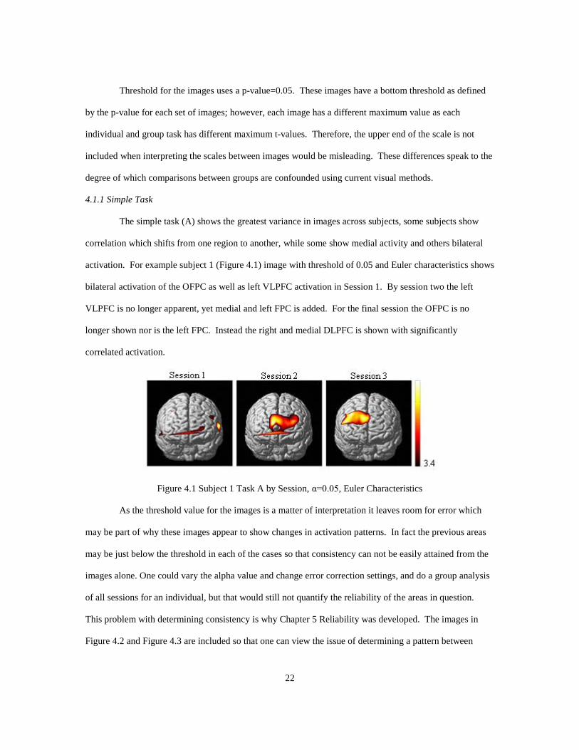
Threshold for the images uses a p-value=0.05. These images have a bottom threshold as defined
by the p-value for each set of images; however, each image has a different maximum value as each
individual and group task has different maximum t-values. Therefore, the upper end of the scale is not
included when interpreting the scales between images would be misleading. These differences speak to the
degree of which comparisons between groups are confounded using current visual methods.
4.1.1 Simple Task
The simple task (A) shows the greatest variance in images across subjects, some subjects show
correlation which shifts from one region to another, while some show medial activity and others bilateral
activation. For example subject 1 (Figure 4.1) image with threshold of 0.05 and Euler characteristics shows
bilateral activation of the OFPC as well as left VLPFC activation in Session 1. By session two the left
VLPFC is no longer apparent, yet medial and left FPC is added. For the final session the OFPC is no
longer shown nor is the left FPC. Instead the right and medial DLPFC is shown with significantly
correlated activation.
Figure 4.1 Subject 1 Task A by Session, α=0.05, Euler Characteristics
As the threshold value for the images is a matter of interpretation it leaves room for error which
may be part of why these images appear to show changes in activation patterns. In fact the previous areas
may be just below the threshold in each of the cases so that consistency can not be easily attained from the
images alone. One could vary the alpha value and change error correction settings, and do a group analysis
of all sessions for an individual, but that would still not quantify the reliability of the areas in question.
This problem with determining consistency is why Chapter 5 Reliability was developed. The images in
Figure 4.2 and Figure 4.3 are included so that one can view the issue of determining a pattern between

23
individual image sessions. Images with “n/a” indicate corrupt data or a missed session. Several images
have no activation within the limits of the threshold specifications such as all sessions for subject four.
Figure 4.2 Simple Task Subjects 1-7 t-map Images, α=0.05, Euler Characteristics

24
Figure 4.3 Simple Task Subjects 8-14 t-map Images, α=0.05, Euler Characteristics
4.1.2 Interference Task
Individual Subject interference task (B) t-maps show larger areas of correlated activation to the
task than the simple task; however, the difficulty with ascertaining a pattern across a subject is still
apparent in Figure 4.4 and Figure 4.5. The increased areas of activation may be an indicator due to the
decreased success rates for the more difficult interference task increasing the required neural activation to
inhibit the distraction of reading the word.

25
Figure 4.4 Interference Task Subjects 1-7 t-map Images, α=0.05, Euler Characteristics

26
Figure 4.5 Interference Task Subjects 8-14 t-map Images, α=0.05, Euler Characteristics
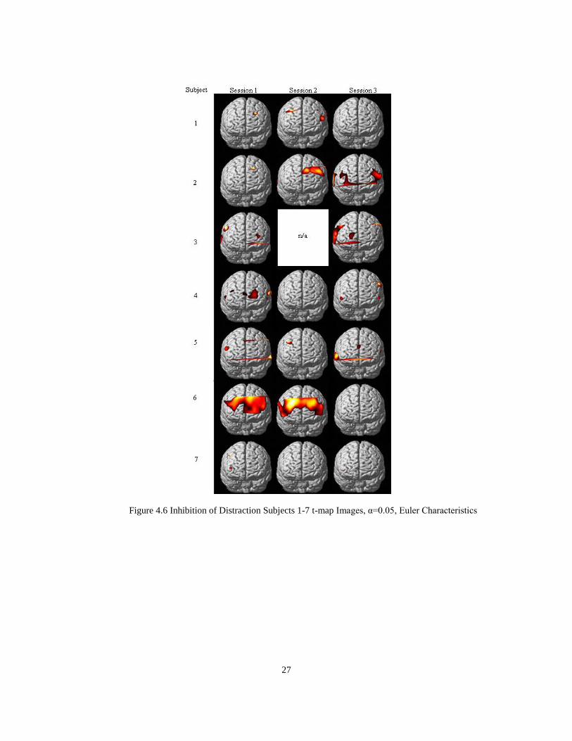
4.1.3 Inhibition of Distraction
The difference between tasks due to the inhibition of distraction (B-A) should also eliminate the
biological noise in this study of saying a color word from the distraction. Areas such as Broca’s area in the
VLPFC should be removed as the activity in that region should theoretically be the same. One marked
exception is subject 14, which also showed to be an outlier in the behavioral analysis.
27
Figure 4.6 Inhibition of Distraction Subjects 1-7 t-map Images, α=0.05, Euler Characteristics

28
Figure 4.7 Inhibition of Distraction Subjects 8-14 t-map Images, α=0.05, Euler Characteristics
4.2 NIRS-SPM Group Analysis
4.2.1 Simple Task
Group Images of the simple task (A) (Figure 4.8) indicates that there is a pattern of activation
consistent across the subjects for medial DLPFC and FPC across sessions as well as activity in the left
motor and temporal cortices (seen as a line on the edge of the left frontal cortex in this frontal view), but it
appears that other areas of activation disappear with time such as the right DLPFC. The type II error

29
correction method for Euler characteristics causes there to be no significant areas to be found and as such is
too conservative a test. Therefore the group analysis images are performed without correction. For Task A
there are no areas above even a 90% threshold with Euler characteristics. The differences in images are
shown for Task B.
Figure 4.8 Group Simple Task t-maps Images, α=0.05, No Correction
4.2.2 Interference Task
Figure 4.9 uses a threshold of 0.05 for an uncorrected image for the group interference task
images. In comparison, Figure 4.10 shows the same data, but with Euler characteristics applied. While the
Euler characteristics works well with individual data, when used with group data too many false negatives
are created. The end result is the image shows no significant areas of activation. It appears from Figure 4.9
that left and right DLPFC and FPC as well as left VMPFC and left motor cortex activity is consistent across
all sessions. Additional comparisons may be viewed in Appendix B.
Figure 4.9 Group Interference Task t-maps Images, α=0.05, No Correction

30
Figure 4.10 Group Interference Task t-maps Images, α=0.05, Euler Characteristics
4.2.3 Inhibition of Distraction
The NIRS-SPM t-map for inhibition of distraction (B-A) (Figure 4.11) shows significant bilateral
DLPFC activity, as well as right side frontal polar (FP) activity for controls, which increases in size with
session 2 to cover the medial DLPFC and decreases with session 3. Independent task imaging also appears
to show the same decrease in activity. This overall trend of reduced activation may be a sign of habituation
as the difference between behavioral tasks approaches 0.
Figure 4.11 Group Inhibition of Distraction t-map Images, α=0.05, No Correction

31
4.2.4 All Sessions Group Images
Group images of all sessions combined to look for those tasks which show matching covariance
across all sessions for each task as shown in Figure 4.12.
Figure 4.12 Group t-maps Images for All Sessions by Task and Correction Method (n=40)

32
Chapter 5
Reliability
Based upon Kolmogorov-Smirnov one-sample testing (Appendix C) only channel 48 was not
normally distributed for Task A, all channels are normally distributed for Task B and for Task B-A
channels 7, 8, 9, 19, 29-32, 42, 45, and 50 were not. While ICC values were calculated for these channels,
their values can not be assumed to be valid as they fail the assumption needed for the ICC calculation. The
HbO values for those channels do not indicate significant correlation to the task and as such have been
ignored. In addition channels 20 and 21 have been ignored as they are not present in the NIRS-SPM frontal
view and as such those channels are not calculated by NIRS-SPM for the frontal view.
As part of the ICC calculation a repeated measures ANOVA is performed across the sessions. The
channels showing significant effect between sessions with 90% confidence for the simple task are 16, 31,
42, and 43. For the interference task, the channels are 17, 35, 36, and 48. No channels showed significant
effect for inhibition of distraction.
All six of the ICC calculations were performed for each channel across sessions (Appendix D);
however, only the two-way random effect with absolute agreement is presented here. As predicted by
Wong, there is little difference given for the data for each of the ICC calculations when good reliability is
shown for any of the calculations. As it is assumed that the sessions and the subjects are random and that
absolute agreement and not just consistency is desired to be compared then the (2,1) and (2,k) calculations
are used. To ease in the recognition of reliable channels the cells have been colored. If the ICC value is
between 0.3 and 0.5, the cell is highlighted in red. If the ICC value is between 0.5 and 0.7, then the cell is
highlighted in yellow. If the ICC value is greater than 0.7, then the cell is highlighted in green as these
cells are clearly in strong agreement. As there are a large number of random cells it may be reasonable to
consider those channels with even moderate reliability as having a lesser degree of connection.

33
5.1 Simple Task Reliability
Those channels which show moderate or better reliability, ICC(2,k) > 0.5, and have a 90%
probability of significant positive or negative normalized mean HbO for the simple task are presented in
Table 5.1.
Table 5.1 Reliable and Significant Channels for the Simple Task
Intraclass Correlation One-Sample t-test
Channel ANOVA
(Sig) (2,1) (2,3) T
Sig
(two-tailed)
9 0.613 0.297 0.560 1.871 0.069
10 0.788 0.225 0.465 5.196 0.00001
15 0.311 0.286 0.546 3.061 0.004
16 0.060 0.360 0.628 2.024 0.050
25 0.571 0.165 0.372 2.074 0.045
26 0.702 0.422 0.686 1.797 0.080
27 0.678 0.188 0.410 2.580 0.014
30 0.422 0.163 0.369 1.724 0.093
31 0.005 0.489 0.742 4.155 0.0002
34 0.855 0.249 0.498 1.760 0.086
42 0.009 0.263 0.518 7.140 0.000000001
45 0.488 0.488 0.741 1.809 0.078
52 0.694 0.599 0.818 3.920 0.0003
While eight channels show moderate to near perfect reliability with significantly positive mean
HbO data for the group (2,3), only channels 16, 31 and 52 also show moderate reliability for the individual
ICC calculation. In addition, repeated measures ANOVA analysis indicates channels 16, 31, and 42 show a
significant interaction between the sessions and the individuals. Figure 5.1 demonstrates the locations with
colored circles corresponding to the ICC value colored cells in Table 5.1. For example channel 15 in the
right DLPFC while having moderate group reliability (0.546) and significant positive data (0.00398) has
poor (2,1) reliability meaning that there is great individual variation. In contrast, channel 52 shows near
perfect group reliability (0.818) with almost strong individual reliability (0.599) and highly significant
positive mean HbO (0.00035.) Channel 9 is located in the premotor/motor cortex and shows poor reliability

34
with a 93.1% probability of positive HbO activity during the task. Channels 26 (medial DLPFC) and 45
(right VLPFC) show strong group reliability and moderate individual reliability with greater than 90%
probability of having positive HbO data. No channels show significant negative mean HbO for this task.
Figure 5.1 Reliable and Significant Channel Locations for the Simple Task
5.2 Interference Task Reliability
The interference task has fourteen channels which meet the reliable and significant criteria, as
shown in Table 5.2. Channels 9, 45, and 52 are not shown in this task as it was in Task A. Channel 52,
while significantly positive for the simple task, is still significantly positive for the interference task but is
not reliable for group data, ICC(2,3)=0.160. Repeated measures ANOVA analysis indicates channels 17,
36, and 48 have significant interaction between individuals and the session. Channels 15 and 26 are shown
as reliably positive between both tasks.

35
Table 5.2 Reliable and Significant Channels for the Interference Task
Intraclass correlation One-Sample t-test
Channel ANOVA
(Sig) (2,1) (2,3) t
Sig
(two-tailed)
13 0.754 0.292 0.553 3.098 0.004
15 0.225 0.49 0.742 3.187 0.003
17 0.055 0.373 0.641 3.511 0.001
25 0.372 0.561 0.793 3.989 0.0002
26 0.715 0.454 0.714 4.081 0.0002
27 0.163 0.527 0.769 4.946 0.00001
28 0.106 0.49 0.742 3.525 0.001
32 0.799 0.452 0.712 2.606 0.013
34 0.356 0.38 0.648 2.605 0.013
36 0.063 0.379 0.647 2.327 0.025
37 0.286 0.262 0.516 1.744 0.089
38 0.179 0.486 0.739 3.181 0.003
39 0.475 0.529 0.771 1.901 0.065
42 0.461 0.333 0.599 7.405 0.00000
46 0.102 0.282 0.541 2.959 0.005
48 0.015 0.416 0.681 2.996 0.005
49 0.616 0.555 0.789 2.787 0.008
Channels 13, 15, and 25 are located in the right DLPFC (Figure 5.2.) Channel 26 is in
the medial DLPFC. Channel 27 and 28 are in the left DLPFC. Channels 34 and 39 are in the right and left
VLPFC respectively. Channel 32 is in the right junction of the temporal, parietal, and motor cortices and
42 at the left junction. Channels 37 and 38 are in the left FPC. Channels 46 and 49 are in the right and left
orbitofrontal cortices.

36
Figure 5.2 Reliable and Significant Channel Locations for the Interference Task
5.3 Inhibition of Distraction Reliability
Changes in neuronal activity due to inhibition of distraction is calculated as the difference between
task mean HbO activity (B-A). Based upon the group reliability criteria shown in Table 5.3, only three
channels show reliable and significantly positive activity at Channels 25, 26 and 27. They are located in
the right and left DLPFC and medial FPC (Figure 5.3.)
Table 5.3 Reliable and Significant Channels for Inhibition of Distraction
Intraclass correlation One-Sample t-test
Channel ANOVA
(Sig) (2,1) (2,3) t
Sig
(two-tailed)
25 0.946 0.266 0.468 1.891 0.066
26 0.463 0.437 0.699 3.199 0.003
27 0.165 0.392 0.659 2.279 0.028

37
Figure 5.3 Reliable and Significant Channel Locations for Inhibition of Distraction

38
Chapter 6
Correlation of HbO to Task Performance
The simple (A) and interference (B) tasks as well as the difference between tasks (B-A), were
correlated using Pearson interclass coefficients. Channels with no sessions having better than a correlation
of 0.30 (fair) are omitted from this chapter for ease of comparison due to the volume of data. Increasingly
darker blue color cells indicate increasing negative correlation while increasingly darker maroon color cells
indicate increasingly positive correlation. A positive correlation means that as the concentration of HbO
increases so does the success rate of the task. A negative correlation means that as the concentration of
HbO increases, the success rate of the task decreases. MNI images for channel locations show an overlay
of this correlation matching the color of the tables.
Table 6.1 HbO to Task Performance for All Sessions
Task
Channel A B B-A
5 -0.46 -0.09 0.01
6 -0.35 -0.03 -0.16
12 -0.31 0.07 -0.15
26 0.08 -0.26 -0.36
28 0.00 -0.17 -0.33
29 -0.02 -0.30 0.14
30 0.08 -0.29 0.21
31 0.18 -0.39 0.19
47 0.02 -0.01 -0.29
50 -0.20 -0.33 -0.02
All sessions were first combined to determine the correlation between HbO and success rates;
however this revealed few channels with only fair correlation (Table 6.1.) As the behavioral data indicated
a significant difference between sessions 1 and 2 and between sessions 1 and 3, each session was then
compared for each of the tasks where possible. While each task shows the correlation values >0.30 only
the values with moderate correlation (>0.50) are generally discussed for the individual sessions.

39
6.1 Simple Task HbO and Performance Correlation
Simple Task Correlation (Table 6.2 and Figure 6.1) initially shows moderate negative correlation
in the superior medial to left DLPFC as well as right posterior DLPFC to right premotor cortex. Session 1
also shows moderate positive correlation in the right FPC. Session 2 for the simple task cannot be
correlated as all of the subjects answered 100% correct. Session 3 and continues to show right and left
DLPFC negative correlation, but also shows right side Wernicke areas to somatosensory cortex and the
right side medial and superior temporal gyri as being positively correlated. The correlation over all
sessions continues to show a weaker negative correlation for the task in the right, left and medial DLPFC.
Also the behavioral analysis revealed that the error rates which are different from 100% success for task A
are outliers so the interpretation of correlation for this task is limited. As task performance improves
activity increases in the right FPC in the first session and right Wernicke and somatosensory cortices, and
right medial and superior temporal gyri in the third session. Also as performance increases activity
decreases in the right premotor cortex and right posterior DLPFC as well as the superior medial to left
DLPFC over all sessions except session 2 which cannot be determined.
Table 6.2 Simple Task %Success correlation to HbO

40
Figure 6.1 Simple Task %Success Correlation to HbO by Session
6.2 Interference Task HbO and Performance Correlation
The interference task shows a fairly negative correlation in Session 1 to the primary
somatosensory cortices close to Wernicke’s area on both the right and left sides. In Session 2 a moderately
negative correlation is observed in the left Broca’s area. Session 3 continues the negative correlation to the
left side Broca’s area and adds left DLPFC and left primary somatosensory cortices. Session 3 also shows a
strong positive correlation to the right side medial and superior temporal gyri as was seen in Session 3 for
the simple task. Therefore as performance increases activity decreases, initially, bilaterally in the
somatosensory cortex, and with repeated sessions shows an increase in the right side medial and temporal
gyri. Also with each session an increasingly larger area in the left DLPFC shows a decrease in activity.
When looking at all sessions combined the left side Broca’s area and somatosensory cortex adjacent to the
auditory cortex and Wernicke’s area show a decrease in activity with an increase in task performance.

41
Table 6.3 Interference Task Correlation to %Success
Figure 6.2 Interference Task %Success Correlation to HbO by Session
6.3 HbO and Performance Correlation for the Inhibitory Response
The correlation of the inhibitory response to the difference in HbO concentrations for the tasks
(Table 6.4 and Figure 6.3) reveals that in the initial session as the inhibitory response increases there is a
moderate correlation to a decrease activity of the medial DLPFC, FPC and OFC, left DLPFC, right
Wernicke and somatosensory cortices, and right medial and superior temporal gyri. However, Session 2

42
indicates that as the inhibitory response increases there is a moderate correlation to an increase in activity in
the left sensory, motor, superior temporal, and premotor cortices, left FPC, bilaterally in the DLPFC, right
OFC and right superior and medial temporal gyri. Session 2 also shows a moderately negative correlation
in the right primary somatosensory cortex. Session 3 shows strong positive correlation to an increase in
inhibitory response in the right side supplementary and premotor cortex, Broca’s area, DLPFC, and right
side superior and medial gyri with a strong negative correlation to the left DLPFC and FPC. When
compared over all sessions only a fairly negative correlation is seen to the inhibitory response in the medial
FPC, OFC, and left DLPFC/Broca’s area.
Table 6.4 Inhibition of Distraction Correlation to HbO Difference
Session Session
Channel 1 2 3 All
Channel 1 2 3 All
1 0.19 -0.41 0.33 0.01 29 -0.45 0.65 -0.38 0.14
2 -0.08 0.24 0.75 0.12
30 -0.22 0.60 -0.27 0.21
3 -0.24 0.40 0.89 0.07
31 -0.14 0.56 -0.15 0.19
4 -0.09 -0.14 0.61 -0.07
32 -0.57 0.56 0.74 0.21
7 -0.02 -0.18 -0.67 -0.04
33 -0.44 0.18 -0.13 -0.01
8 -0.05 -0.03 -0.32 0.00 35 -0.12 0.42 -0.27 0.04
9 0.01 -0.35 0.003 -0.02 36 -0.04 0.31 -0.02 0.06
10 -0.23 0.53 -0.20 0.15 37 -0.17 0.49 0.31 0.03
11 -0.17 -0.51 0.31 -0.19
38 -0.34 0.26 0.03 -0.03
12 -0.41 0.23 0.05 -0.15 40 -0.37 0.55 -0.24 0.12
13 0.11 0.21 0.70 0.20
41 -0.36 0.49 -0.30 0.14
15 -0.03 0.58 -0.10 0.15 42 -0.13 0.59 -0.14 0.23
16 -0.19 0.42 -0.62 0.04
43 -0.53 0.42 0.10 0.12
17 -0.14 0.53 -0.68 -0.06
45 -0.13 0.36 -0.25 0.03
18 -0.15 -0.40 -0.11 -0.17
46 -0.25 0.64 -0.47 0.08
19 -0.11 0.60 0.12 0.24 47 -0.58 0.02 -0.03 -0.29
22 -0.58 0.34 0.04 0.03
48 -0.38 0.60 0.20 0.15
24 -0.14 -0.33 0.03 -0.17 49 -0.62 0.45 -0.18 -0.17
25 -0.21 0.49 -0.47 0.00
50 -0.36 0.41 -0.35 -0.02
26 -0.59 -0.03 -0.28 -0.36
51 -0.36 0.55 -0.32 0.11
27 -0.28 0.46 -0.76 -0.08 52 -0.15 0.55 -0.12 0.18
28 -0.45 -0.15 -0.42 -0.33

43
Figure 6.3 Inhibition of Distraction Correlation to HbO Difference by Session

44
Chapter 7
Discussion
Behavioral analysis indicates a significant difference between the initial session and the other two
sessions only for the interference task and between tasks for Session 2. Qualitatively the NIRS-SPM t-maps
show regions of interest which are difficult to quantify over time even with sessions over time. It can not
be seen by those images alone if the covariance of a single session outweighs others by giving extra weight
to the values where there should not be. By combining the group analysis methodology for reliability as a
transparent overlay on top of the NIRS-SPM images (Figure 7.1) and further comparison to the correlation
of task success to changes in oxygenation several inferences can be made.
Figure 7.1 Group t-maps for All Sessions by Task with Reliability Overlay
7.1 Simple Task
For the simple task, the most significantly correlated areas using the t-map methodology are from
Wernicke’s to Broca’s areas on the left side. As may be expected for a simple speech task, the left middle
temporal gyrus and the right Broca’s area and DLPFC demonstrate strong reliability and significant areas
of covariance of activation to the task, and left premotor cortex show moderate reliability. What is novel, is
that the medial FPC and DLPFC show significant covariance to the task with moderate reliability.
Bilaterally the DLPFC shows significant covariance to the simple task, but there is enough variation among

45
sessions and individuals to lead to a fair to poor reliability in these regions. Most of the regions outside of
the t-map threshold area yet within the probe area show random data with no correlation; however, the
superior medial DLPFC, superior left DLPFC, and right premotor cortex, do show fairly negative
correlation of HbO concentration to task success. Also, the right FPC shows an increase HbO
concentration with task success on the initial presentation of an oral Stroop task while the middle temporal
gyrus with repeated sessions. Finally, these correlations taken together infer that while bilateral activation
of the DLPFC and FPC show significant covariance to the task, bilateral activation of the cortices
responsible for speech, right side deactivation of the sensory cortex, and deactivation of the medial DLPFC
are important for success in this task.
7.2 Interference Task
The interference task shows a larger area of significant covariance and reliability than the simple
task with the strongly reliable channels located in the right and left DLPFC/FPC, left VLPFC, left OFC,
and right medial/superior temporal gyrus. The reliability of the cortices within the threshold of the t-map
image also show moderate to strong group reliability. Bilateral deactivation of the somatosensory cortices
initially shows fair correlation to task success. Repeated sessions show moderate correlation of
deactivation of the left premotor cortex and left DLPFC and activation of the right medial temporal gyrus to
task success.
Cortical areas related to speech on the left hand side are not as reliably activated for the
interference task as they were for the simple task; however medial and right FPC/DLPFC shows an even
greater consistency for activation while also showing strong reliability for the left FPC/DLPFC. Finally,
both tasks show increased activity in the medial temporal gyrus shows increased success in the third
session.
7.3 Inhibition of Distraction
Inhibition of Distraction shows significant covariance bilaterally in the DLPFC and FPC; however
it is moderate to strongly consistent across repeated sessions only in the superior regions of the medial and
left FPC while only being fairly consistent in the right FPC. The lack of consistency for the bilateral
inferior FPC and right DLPFC leading to Broca’s area can be accounted for in the changing poor positive

46
to negative correlation of the inhibitory response as well as the individual tasks to HbO concentration of
those areas with repeated sessions. Finally, as each session is repeated, the right DLPFC shows
increasingly positive correlation to the inhibitory response while the left DLPFC shows an increasingly
negative correlation to the inhibitory response.
7.4 Conclusion
While NIRS-SPM group t-maps provide a view of the channels which show the covariance of the
task to the changes in HbO, it does not directly provide a way to determine which channels can be reliably
shown as being consistently activated in any given session. Channel-wise intraclass-correlation analysis
provides a method by which the degree of consistent reliability can be seen within the regions of significant
activity. In addition those regions which may be otherwise seen as random or of poorer reliability for HbO
concentrations may instead show correlation to the task success. In contrast, those areas which indicate
high covariance of HbO to the task protocol may show a high degree of variance with individual subject
differences and sessions. Therefore, reliability of the data must be considered when looking at repeated
sessions for a functional imaging study.
Inhibition of distraction shows moderate to strong reliability in the medial and left DLPFC and
FPC for HbO activation. In addition as the inhibitory response increases, HbO decreases in the medial
DLPFC/FPC and left DLPFC. These channel locations can be compared to patient data on a group basis
and may be sufficiently reliable for individual comparisons. A pattern of increasing positive correlation in
the right DLPFC and negative correlation in the left DLPFC/FPC could also be used, but more sessions
may be required to do so. Modifying the protocol to record patient’s auditory response with timestamp
device would also allow for correlation between HbO and the subject’s response time. The response time
may explain those channels which change in activation during different sessions and determine areas of
correlation when the subjects achieve 100% success. It may provide an adequate measure for more than
three sessions to be compared as the subject may show a delayed response while still successfully
indicating the color. Extending this methodology as a full automated layer of transparency within NIRS-
SPM would aid clinicians by providing a basis to compare other patient groups and determine individual
responses to treatment.

47
Appendix A
Brodmann Anatomical References to Channels

48
The table below is broken down by channel and shows the percentage of Brodmann area coverage
in which the channel resides along with the anatomical area. Overlap refers to what percentage of the
channel is in the region listed.
Channel Brodmann Anatomical Label Overlap
1 1 Primary Somatosensory Cortex 38.9%
1 2 Primary Somatosensory Cortex 5.3%
1 3 Primary Somatosensory Cortex 23.9%
1 4 Primary Motor Cortex 17.9%
1 43 Subcentral area 14.0%
2 6 Pre-Motor and Supplementary Motor Cortex 60.0%
2 9 Dorsolateral prefrontal cortex 15.3%
2 44 pars opercularis (Broca's area) 24.7%
3 9 Dorsolateral prefrontal cortex 62.2%
3 44 pars opercularis (Broca's area) 20.4%
3 45 pars triangularis Broca's area 11.7%
3 46 Dorsolateral prefrontal cortex 5.7%
4 9 Dorsolateral prefrontal cortex 100.0%
5 8 Includes Frontal eye fields 3.3%
5 9 Dorsolateral prefrontal cortex 96.7%
6 9 Dorsolateral prefrontal cortex 100.0%
7 8 Includes Frontal eye fields 2.3%
7 9 Dorsolateral prefrontal cortex 91.0%
7 45 pars triangularis Broca's area 0.9%
7 46 Dorsolateral prefrontal cortex 5.9%
8 6 Pre-Motor and Supplementary Motor Cortex 11.0%
8 9 Dorsolateral prefrontal cortex 49.8%
8 44 pars opercularis (Broca's area) 39.2%
9 1 Primary Somatosensory Cortex 1.5%
9 3 Primary Somatosensory Cortex 18.7%
9 4 Primary Motor Cortex 35.1%
9 6 Pre-Motor and Supplementary Motor Cortex 41.8%
9 43 Subcentral area 3.0%
10 1 Primary Somatosensory Cortex 19.6%
10 2 Primary Somatosensory Cortex 24.6%
10 3 Primary Somatosensory Cortex 13.8%
10 40 Supramarginal gyrus part of Wernicke's area 42.0%
11 1 Primary Somatosensory Cortex 6.9%

49
11 2 Primary Somatosensory Cortex 79.4%
11 40 Supramarginal gyrus part of Wernicke's area 13.7%
12 3 Primary Somatosensory Cortex 0.3%
12 4 Primary Motor Cortex 9.6%
12 6 Pre-Motor and Supplementary Motor Cortex 34.6%
12 43 Subcentral area 55.5%
13 44 pars opercularis (Broca's area) 50.9%
13 45 pars triangularis Broca's area 49.1%
14 9 Dorsolateral prefrontal cortex 18.5%
14 45 pars triangularis Broca's area 28.2%
14 46 Dorsolateral prefrontal cortex 53.2%
15 9 Dorsolateral prefrontal cortex 76.5%
15 10 Frontopolar area 17.8%
15 46 Dorsolateral prefrontal cortex 5.7%
16 9 Dorsolateral prefrontal cortex 72.7%
16 10 Frontopolar area 27.3%
17 9 Dorsolateral prefrontal cortex 49.3%
17 46 Dorsolateral prefrontal cortex 50.7%
18 9 Dorsolateral prefrontal cortex 1.6%
18 44 pars opercularis (Broca's area) 18.5%
18 45 pars triangularis Broca's area 69.4%
18 46 Dorsolateral prefrontal cortex 10.5%
19 4 Primary Motor Cortex 8.9%
19 6 Pre-Motor and Supplementary Motor Cortex 67.4%
19 43 Subcentral area 2.2%
19 44 pars opercularis (Broca's area) 21.5%
20 1 Primary Somatosensory Cortex 30.7%
20 2 Primary Somatosensory Cortex 35.3%
20 3 Primary Somatosensory Cortex 4.2%
20 43 Subcentral area 28.8%
20 48 Retrosubicular area 1.0%
21 2 Primary Somatosensory Cortex 6.4%
21 40 Supramarginal gyrus part of Wernicke's area 76.6%
21 48 Retrosubicular area 17.0%
22 2 Primary Somatosensory Cortex 4.0%
22 22 Superior Temporal Gyrus 39.0%
22 43 Subcentral area 56.0%
22 48 Retrosubicular area 0.9%
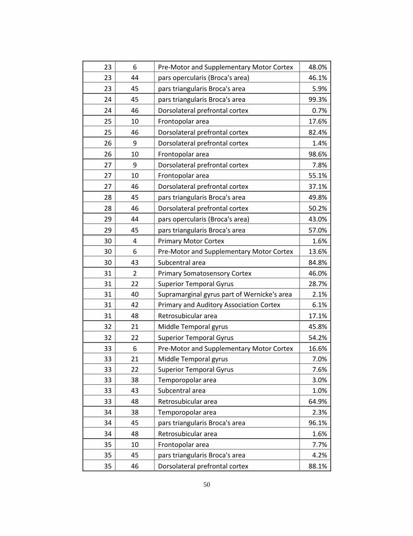
50
23 6 Pre-Motor and Supplementary Motor Cortex 48.0%
23 44 pars opercularis (Broca's area) 46.1%
23 45 pars triangularis Broca's area 5.9%
24 45 pars triangularis Broca's area 99.3%
24 46 Dorsolateral prefrontal cortex 0.7%
25 10 Frontopolar area 17.6%
25 46 Dorsolateral prefrontal cortex 82.4%
26 9 Dorsolateral prefrontal cortex 1.4%
26 10 Frontopolar area 98.6%
27 9 Dorsolateral prefrontal cortex 7.8%
27 10 Frontopolar area 55.1%
27 46 Dorsolateral prefrontal cortex 37.1%
28 45 pars triangularis Broca's area 49.8%
28 46 Dorsolateral prefrontal cortex 50.2%
29 44 pars opercularis (Broca's area) 43.0%
29 45 pars triangularis Broca's area 57.0%
30 4 Primary Motor Cortex 1.6%
30 6 Pre-Motor and Supplementary Motor Cortex 13.6%
30 43 Subcentral area 84.8%
31 2 Primary Somatosensory Cortex 46.0%
31 22 Superior Temporal Gyrus 28.7%
31 40 Supramarginal gyrus part of Wernicke's area 2.1%
31 42 Primary and Auditory Association Cortex 6.1%
31 48 Retrosubicular area 17.1%
32 21 Middle Temporal gyrus 45.8%
32 22 Superior Temporal Gyrus 54.2%
33 6 Pre-Motor and Supplementary Motor Cortex 16.6%
33 21 Middle Temporal gyrus 7.0%
33 22 Superior Temporal Gyrus 7.6%
33 38 Temporopolar area 3.0%
33 43 Subcentral area 1.0%
33 48 Retrosubicular area 64.9%
34 38 Temporopolar area 2.3%
34 45 pars triangularis Broca's area 96.1%
34 48 Retrosubicular area 1.6%
35 10 Frontopolar area 7.7%
35 45 pars triangularis Broca's area 4.2%
35 46 Dorsolateral prefrontal cortex 88.1%

51
36 10 Frontopolar area 100.0%
37 10 Frontopolar area 100.0%
38 10 Frontopolar area 41.5%
38 46 Dorsolateral prefrontal cortex 58.5%
39 45 pars triangularis Broca's area 90.2%
39 46 Dorsolateral prefrontal cortex 9.8%
40 6 Pre-Motor and Supplementary Motor Cortex 47.6%
40 44 pars opercularis (Broca's area) 31.3%
40 45 pars triangularis Broca's area 0.7%
40 48 Retrosubicular area 20.5%
41 21 Middle Temporal gyrus 1.6%
41 22 Superior Temporal Gyrus 80.9%
41 43 Subcentral area 12.2%
41 48 Retrosubicular area 5.3%
42 21 Middle Temporal gyrus 6.8%
42 22 Superior Temporal Gyrus 92.9%
42 42 Primary and Auditory Association Cortex 0.3%
43 21 Middle Temporal gyrus 97.1%
43 22 Superior Temporal Gyrus 2.9%
44 38 Temporopolar area 88.4%
44 48 Retrosubicular area 11.6%
45 45 pars triangularis Broca's area 25.0%
45 46 Dorsolateral prefrontal cortex 62.2%
45 47 Inferior prefrontal gyrus 12.8%
46 10 Frontopolar area 40.8%
46 11 Orbitofrontal area 55.0%
46 46 Dorsolateral prefrontal cortex 0.3%
46 47 Inferior prefrontal gyrus 3.8%
47 10 Frontopolar area 81.7%
47 11 Orbitofrontal area 18.3%
48 10 Frontopolar area 52.6%
48 11 Orbitofrontal area 47.4%
49 10 Frontopolar area 6.8%
49 45 pars triangularis Broca's area 1.5%
49 46 Dorsolateral prefrontal cortex 91.6%
50 38 Temporopolar area 26.8%
50 45 pars triangularis Broca's area 67.1%
50 47 Inferior prefrontal gyrus 0.6%

52
50 48 Retrosubicular area 5.4%
51 21 Middle Temporal gyrus 50.0%
51 22 Superior Temporal Gyrus 4.3%
51 38 Temporopolar area 7.3%
51 48 Retrosubicular area 38.3%
52 20 Inferior Temporal gyrus 0.3%
52 21 Middle Temporal gyrus 90.1%
52 22 Superior Temporal Gyrus 9.6%

53
Appendix B
Group NIRS-SPM t-maps

54
To decide upon the optimal threshold settings, several different views of the image were
performed using different numbers of sessions combined, correction type, and alpha threshold. What
follows are those different image settings for each task as well as a copy of the image without any
threshold.
Group (with no correction)
Task Session 1 (n=14) Session 2 (n=13) Session 3 (n=13)
A
B
B-A

55
Control Group Task B (Without and With Euler Characteristics)
Task Session 1 (n=14) Session 2 (n=13) Session 3 (n=13)
No
Correction
Euler
No significant areas

56
Task A for all Sessions and varied threshold
Threshold α = 0.10 α = 0.05 α = 0.01
EC
No
Correction
No
Threshold

57
Task B for All Sessions and varied threshold
Threshold α = 0.10 α = 0.05 α = 0.01
EC
No Correction
No Threshold

58
Task B-A for All Sessions and varied threshold
Threshold α = 0.10 α = 0.05 α = 0.01
Euler
No significant areas
No Correction
No Threshold

59
Task A for Sessions 2 and 3 and varied threshold
Threshold α = 0.10 α = 0.05 α = 0.01
Euler
No Correction
No Threshold

60
Task B for Sessions 2 and 3 and varied threshold
Threshold α = 0.10 α = 0.05 α = 0.01
Euler
No Correction
No Threshold

61
Task B-A for Sessions 2 and 3 and varied threshold
Threshold α = 0.10 α = 0.05 α = 0.01
Euler No significant areas No significant areas No significant areas
No Correction
No Threshold

62
Appendix C
Kolmogorov-Smirnov One Sample Tests

63
The Kolmogorov-Smirnov one-sample test is used to determine if a data set follows a normal
distribution. Below is the output from IBM SPSS for all channels except channel 20 and 21 for each
session. Digits before the period are the channel number. The digit after the period is the session. Letters
refer to Task A, B or B-A. A significance value less than 0.05 means the data has 95% confidence of the
data not having a normal distribution and the decision is highlighted in yellow when this hypothesis is
violated.

64

65

66

67

68

69

70

71

72

73

74

75

76

77
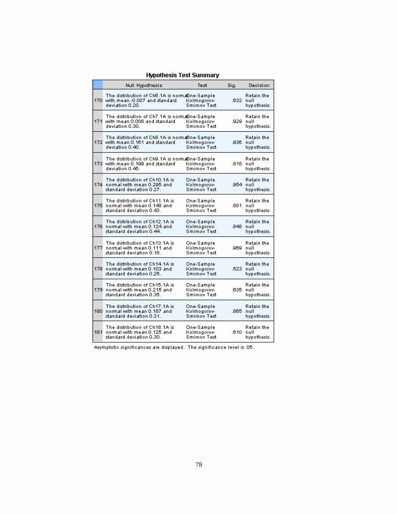
78

79

80

81

82

83

84

85

86

87

88

89

90

91

92

93

94

95

96

97

98

99

100

101

102
Appendix D
Channel-wise Statistics

103
Intraclass Correlation for all six of Shrout and Fleiss models are given below as calculated in
Matlab. These values were compared to SPSS as suggested by Wong and the values are equivalent. A
channel and task shaded in yellow indicates that the data for that task and channel for at least one session
failed the Kolmogorov-Smirnov test (Appendix C.) Yellow entries for ANOVA indicate a significance of
90% or greater chance of an interaction effect across sessions. A red line around the ANOVA cell indicates
there is greater than a 95% chance of an interaction effect across sessions. For ICC calculations a red cell
indicates values between 0.3 and 0.5, yellow indicates between 0.5 and 0.7 and green indicates values
greater than 0.7. For one-sample t-test values those showing 90% to 95% probability of a significant
positive or negative values (as indicated by the t-value), while green indicates a 95% or greater probability.
ICC (1,1) and (1,k) refer to one-way random effects analysis, (2,1) and (2,k) refer to two-way random
effects analysis with absolute agreement, while (3,1) and (3,k) refer to two-way mixed effect analysis with
consistency.
Intraclass Correlation One-sample
Ch Task ANOVA (1,1) (2,1) (3,1) (1,k) (2,k) (3,k) t-value p-value
1 A 0.203 0.042 0.058 0.062 0.115 0.157 0.165 1.573 0.124
2 A 0.077 -0.187 -0.127 -0.150 -0.898 -0.509 -0.641 0.540 0.592
3 A 0.274 -0.090 -0.079 -0.081 -0.331 -0.280 -0.291 1.121 0.269
4 A 0.101 -0.068 -0.026 -0.030 -0.236 -0.083 -0.095 1.482 0.146
5 A 0.14 -0.085 -0.052 -0.057 -0.309 -0.174 -0.194 1.506 0.140
6 A 0.131 0.122 0.146 0.158 0.295 0.338 0.361 0.671 0.506
7 A 0.971 -0.122 -0.160 -0.145 -0.485 -0.708 -0.616 -0.533 0.597
8 A 0.141 -0.052 -0.021 -0.023 -0.173 -0.064 -0.071 -0.368 0.715
9 A 0.613 0.305 0.297 0.289 0.568 0.560 0.549 1.871 0.069
10 A 0.788 0.238 0.225 0.213 0.484 0.465 0.449 5.196 0.000
11 A 0.594 0.101 0.090 0.087 0.252 0.228 0.221 0.801 0.428
12 A 0.448 0.249 0.246 0.244 0.498 0.495 0.491 -0.329 0.744
13 A 0.424 -0.109 -0.113 -0.112 -0.418 -0.436 -0.431 2.219 0.032
14 A 0.287 -0.064 -0.055 -0.056 -0.222 -0.184 -0.190 0.972 0.337
15 A 0.311 0.283 0.286 0.290 0.542 0.546 0.550 3.061 0.004
16 A 0.06 0.338 0.360 0.400 0.605 0.628 0.667 2.024 0.050
17 A 0.373 -0.065 -0.064 -0.064 -0.225 -0.221 -0.222 1.862 0.070
18 A 0.245 -0.242 -0.222 -0.233 -1.410 -1.199 -1.314 0.947 0.350
19 A 0.816 -0.052 -0.079 -0.073 -0.175 -0.282 -0.258 -0.363 0.718
22 A 0.675 0.186 0.175 0.167 0.407 0.388 0.376 -0.363 0.719

104
23 A 0.693 0.287 0.277 0.267 0.547 0.535 0.522 0.703 0.487
24 A 0.155 0.030 0.054 0.058 0.084 0.146 0.157 1.961 0.057
25 A 0.571 0.173 0.165 0.160 0.386 0.372 0.363 2.074 0.045
26 A 0.702 0.428 0.422 0.408 0.692 0.686 0.674 1.797 0.080
27 A 0.678 0.199 0.188 0.180 0.427 0.410 0.397 2.580 0.014
28 A 0.295 -0.010 -0.002 -0.002 -0.030 -0.005 -0.005 1.550 0.129
29 A 0.441 -0.044 -0.048 -0.048 -0.143 -0.160 -0.157 0.625 0.536
30 A 0.422 0.165 0.163 0.162 0.373 0.369 0.367 1.724 0.093
31 A 0.005 0.459 0.489 0.585 0.718 0.742 0.809 4.155 0.000
32 A 0.083 0.571 0.578 0.612 0.800 0.805 0.826 1.140 0.261
33 A 0.553 0.237 0.231 0.225 0.483 0.474 0.465 -0.613 0.543
34 A 0.855 0.263 0.249 0.235 0.517 0.498 0.480 1.760 0.086
35 A 0.759 -0.003 -0.025 -0.023 -0.009 -0.079 -0.074 1.242 0.222
36 A 0.285 0.316 0.320 0.326 0.581 0.586 0.592 -0.547 0.588
37 A 0.583 0.199 0.190 0.184 0.426 0.413 0.404 0.633 0.530
38 A 0.213 0.169 0.181 0.189 0.379 0.398 0.411 1.564 0.126
39 A 0.115 0.245 0.264 0.286 0.494 0.519 0.546 -0.532 0.598
40 A 0.214 -0.053 -0.034 -0.036 -0.179 -0.111 -0.117 0.799 0.429
41 A 0.401 0.306 0.305 0.304 0.569 0.568 0.568 1.207 0.235
42 A 0.009 0.207 0.263 0.334 0.440 0.518 0.601 7.140 0.000
43 A 0.068 0.492 0.505 0.544 0.744 0.754 0.782 0.199 0.843
44 A 0.213 0.080 0.095 0.099 0.207 0.239 0.248 1.079 0.287
45 A 0.488 0.490 0.488 0.483 0.743 0.741 0.737 1.809 0.078
46 A 0.482 0.002 -0.005 -0.005 0.005 -0.016 -0.015 0.020 0.984
47 A 0.297 0.012 0.020 0.020 0.036 0.057 0.058 -0.279 0.782
48 A 0.167 0.117 0.136 0.145 0.285 0.320 0.337 -0.146 0.885
49 A 0.096 0.014 0.051 0.058 0.042 0.139 0.155 -0.069 0.945
50 A 0.44 0.047 0.043 0.043 0.129 0.119 0.118 0.075 0.941
51 A 0.528 0.071 0.062 0.061 0.186 0.166 0.162 2.427 0.020
52 A 0.694 0.602 0.599 0.586 0.819 0.818 0.809 3.920 0.000
1 B 0.449 -0.047 -0.053 -0.052 -0.157 -0.176 -0.173 2.208 0.033
2 B 0.951 0.140 0.119 0.110 0.329 0.288 0.271 1.496 0.143
3 B 0.982 -0.053 -0.087 -0.080 -0.179 -0.318 -0.285 1.962 0.057
4 B 0.575 0.253 0.246 0.239 0.504 0.494 0.485 1.740 0.090
5 B 0.768 0.094 0.076 0.072 0.238 0.198 0.188 0.449 0.656
6 B 0.785 0.295 0.284 0.271 0.557 0.543 0.527 0.905 0.371
7 B 0.567 0.212 0.204 0.199 0.446 0.435 0.426 -1.017 0.315
8 B 0.834 0.032 0.009 0.008 0.090 0.025 0.024 -0.473 0.639
9 B 0.837 0.056 0.033 0.031 0.150 0.094 0.088 1.139 0.262
10 B 0.666 0.063 0.048 0.045 0.167 0.130 0.125 5.975 0.000

105
11 B 0.718 -0.233 -0.264 -0.246 -1.312 -1.674 -1.447 3.002 0.005
12 B 0.679 0.530 0.526 0.513 0.772 0.769 0.759 0.352 0.726
13 B 0.754 0.303 0.292 0.280 0.566 0.553 0.538 3.098 0.004
14 B 0.421 0.084 0.082 0.081 0.216 0.210 0.209 2.975 0.005
15 B 0.225 0.486 0.490 0.502 0.739 0.742 0.752 3.187 0.003
16 B 0.934 0.431 0.126 0.406 0.694 0.301 0.672 2.852 0.007
17 B 0.055 0.351 0.373 0.415 0.618 0.641 0.680 3.511 0.001
18 B 0.196 0.084 0.100 0.106 0.215 0.250 0.262 1.817 0.077
19 B 0.631 0.022 0.007 0.007 0.064 0.021 0.020 0.791 0.434
22 B 0.772 0.360 0.351 0.336 0.628 0.618 0.603 0.918 0.364
23 B 0.88 0.249 0.234 0.221 0.499 0.479 0.460 1.412 0.166
24 B 0.168 -0.206 -0.172 -0.188 -1.053 -0.787 -0.904 5.244 0.000
25 B 0.372 0.561 0.561 0.562 0.793 0.793 0.794 3.989 0.000
26 B 0.715 0.460 0.454 0.440 0.719 0.714 0.702 4.081 0.000
27 B 0.163 0.521 0.527 0.546 0.765 0.769 0.783 4.946 0.000
28 B 0.106 0.480 0.490 0.519 0.735 0.742 0.764 3.525 0.001
29 B 0.243 0.059 0.071 0.074 0.158 0.186 0.192 2.397 0.021
30 B 0.622 0.038 0.023 0.022 0.105 0.067 0.064 2.003 0.052
31 B 0.921 0.206 0.189 0.177 0.438 0.411 0.392 4.367 0.000
32 B 0.799 0.459 0.452 0.436 0.718 0.712 0.698 2.606 0.013
33 B 0.732 0.213 0.200 0.191 0.448 0.429 0.414 -0.247 0.806
34 B 0.356 0.379 0.380 0.382 0.647 0.648 0.649 2.605 0.013
35 B 0.407 0.094 0.092 0.092 0.237 0.234 0.233 3.993 0.000
36 B 0.063 0.500 0.379 0.564 0.750 0.647 0.795 2.327 0.025
37 B 0.286 0.258 0.262 0.268 0.510 0.516 0.523 1.744 0.089
38 B 0.179 0.480 0.486 0.503 0.734 0.739 0.752 3.181 0.003
39 B 0.475 0.530 0.529 0.524 0.772 0.771 0.767 1.901 0.065
40 B 0.826 0.008 -0.016 -0.015 0.024 -0.050 -0.047 0.683 0.498
41 B 0.56 0.044 0.033 0.032 0.122 0.094 0.091 0.817 0.419
42 B 0.461 0.335 0.333 0.329 0.602 0.599 0.596 7.405 0.000
43 B 0.687 0.165 0.152 0.145 0.371 0.349 0.337 0.247 0.806
44 B 0.806 0.210 0.195 0.185 0.444 0.421 0.405 0.591 0.558
45 B 0.388 -0.057 -0.057 -0.057 -0.192 -0.193 -0.193 4.268 0.000
46 B 0.102 0.262 0.282 0.307 0.516 0.541 0.571 2.959 0.005
47 B 0.206 0.266 0.276 0.287 0.521 0.533 0.547 1.424 0.162
48 B 0.015 0.385 0.416 0.488 0.653 0.681 0.741 2.996 0.005
49 B 0.616 0.557 0.555 0.544 0.791 0.789 0.782 2.787 0.008
50 B 0.87 -0.047 -0.076 -0.070 -0.156 -0.269 -0.245 1.627 0.112
51 B 0.791 0.010 -0.013 -0.012 0.030 -0.039 -0.036 1.358 0.182
52 B 0.981 0.085 0.060 0.055 0.219 0.160 0.149 3.212 0.003

106
1 B-A 0.959 0.102 0.078 0.073 0.255 0.203 0.190 0.272 0.787
2 B-A 0.68 -0.137 -0.160 -0.151 -0.566 -0.709 -0.650 0.665 0.510
3 B-A 0.833 -0.340 -0.386 -0.350 -3.200 -5.506 -3.507 1.081 0.286
4 B-A 0.957 0.354 0.342 0.324 0.622 0.609 0.589 0.737 0.465
5 B-A 0.212 0.270 0.279 0.290 0.525 0.537 0.550 -0.005 0.996
6 B-A 0.296 0.297 0.301 0.306 0.559 0.564 0.570 1.326 0.192
7 B-A 0.504 -0.011 -0.020 -0.019 -0.034 -0.061 -0.059 -1.308 0.199
8 B-A 0.233 -0.159 -0.139 -0.147 -0.697 -0.578 -0.622 -0.869 0.390
9 B-A 0.578 -0.211 -0.230 -0.220 -1.095 -1.275 -1.174 -0.886 0.381
10 B-A 0.923 0.028 0.001 0.001 0.080 0.004 0.004 0.521 0.605
11 B-A 0.941 0.024 -0.004 -0.003 0.069 -0.011 -0.010 1.218 0.231
12 B-A 0.772 0.116 0.099 0.094 0.283 0.248 0.236 -1.135 0.263
13 B-A 0.737 0.031 0.012 0.011 0.088 0.034 0.032 0.393 0.696
14 B-A 0.506 -0.027 -0.036 -0.035 -0.086 -0.117 -0.114 2.068 0.045
15 B-A 0.384 0.096 0.096 0.096 0.241 0.241 0.241 0.636 0.528
16 B-A 0.141 0.061 0.085 0.093 0.162 0.219 0.235 2.268 0.029
17 B-A 0.754 0.326 0.316 0.303 0.592 0.581 0.566 1.187 0.242
18 B-A 0.371 -0.042 -0.041 -0.041 -0.137 -0.133 -0.133 -0.170 0.866
19 B-A 0.802 -0.070 -0.097 -0.090 -0.245 -0.362 -0.331 -0.711 0.481
22 B-A 0.147 0.034 0.060 0.065 0.096 0.160 0.172 -1.039 0.305
23 B-A 0.736 -0.032 -0.054 -0.050 -0.101 -0.180 -0.168 -1.314 0.197
24 B-A 0.209 -0.069 -0.048 -0.051 -0.239 -0.161 -0.172 2.460 0.018
25 B-A 0.946 0.243 0.226 0.212 0.491 0.468 0.447 1.891 0.066
26 B-A 0.463 0.438 0.437 0.432 0.701 0.699 0.696 3.199 0.003
27 B-A 0.165 0.383 0.392 0.411 0.651 0.659 0.676 2.279 0.028
28 B-A 0.622 0.345 0.338 0.329 0.612 0.605 0.595 1.325 0.193
29 B-A 0.756 -0.051 -0.075 -0.071 -0.172 -0.266 -0.246 -0.412 0.683
30 B-A 0.338 -0.052 -0.047 -0.048 -0.173 -0.157 -0.159 -0.903 0.372
31 B-A 0.251 -0.045 -0.032 -0.033 -0.149 -0.101 -0.105 -0.629 0.533
32 B-A 0.298 -0.073 -0.064 -0.066 -0.255 -0.220 -0.226 -0.629 0.533
33 B-A 0.231 -0.044 -0.028 -0.029 -0.145 -0.088 -0.093 -1.664 0.104
34 B-A 0.631 0.143 0.132 0.127 0.334 0.313 0.303 -1.060 0.296
35 B-A 0.762 0.069 0.050 0.047 0.182 0.137 0.130 1.056 0.298
36 B-A 0.218 -0.209 -0.185 -0.197 -1.081 -0.884 -0.976 2.674 0.011
37 B-A 0.114 0.117 0.143 0.157 0.284 0.334 0.359 0.359 0.722
38 B-A 0.6 0.206 0.198 0.191 0.438 0.425 0.415 0.405 0.688
39 B-A 0.525 0.230 0.224 0.219 0.472 0.464 0.457 1.358 0.182
40 B-A 0.531 -0.133 -0.146 -0.141 -0.544 -0.618 -0.590 -1.514 0.138
41 B-A 0.33 -0.087 -0.082 -0.083 -0.317 -0.293 -0.299 -1.485 0.146
42 B-A 0.295 -0.066 -0.057 -0.059 -0.229 -0.194 -0.200 -0.756 0.454
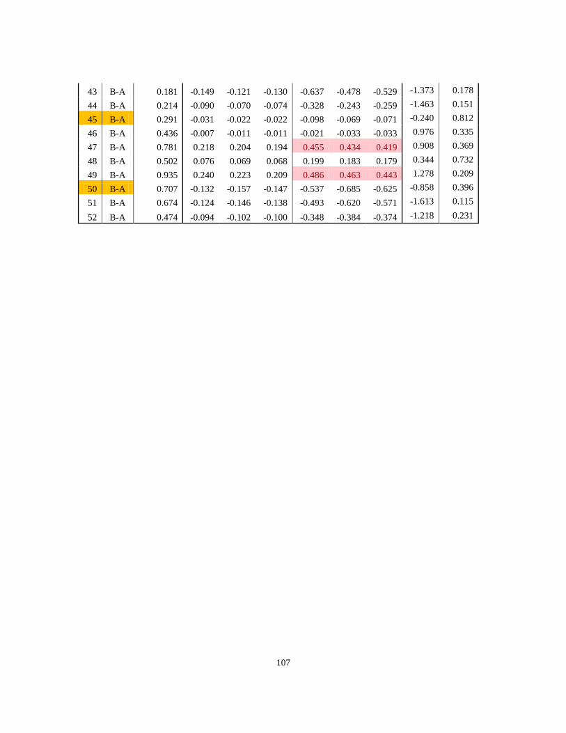
107
43 B-A 0.181 -0.149 -0.121 -0.130 -0.637 -0.478 -0.529 -1.373 0.178
44 B-A 0.214 -0.090 -0.070 -0.074 -0.328 -0.243 -0.259 -1.463 0.151
45 B-A 0.291 -0.031 -0.022 -0.022 -0.098 -0.069 -0.071 -0.240 0.812
46 B-A 0.436 -0.007 -0.011 -0.011 -0.021 -0.033 -0.033 0.976 0.335
47 B-A 0.781 0.218 0.204 0.194 0.455 0.434 0.419 0.908 0.369
48 B-A 0.502 0.076 0.069 0.068 0.199 0.183 0.179 0.344 0.732
49 B-A 0.935 0.240 0.223 0.209 0.486 0.463 0.443 1.278 0.209
50 B-A 0.707 -0.132 -0.157 -0.147 -0.537 -0.685 -0.625 -0.858 0.396
51 B-A 0.674 -0.124 -0.146 -0.138 -0.493 -0.620 -0.571 -1.613 0.115
52 B-A 0.474 -0.094 -0.102 -0.100 -0.348 -0.384 -0.374 -1.218 0.231

108
References
1U.S. Centers for Disease Control and Prevention, “Injury Prevention and Control: Traumatic Brain Injury”
http://www.cdc.gov/TraumaticBrainInjury/index.html, July 2013.
2Luria, A.R., “Higher Cortical Functions in Man,” Basic Books, NY, 1966.
3Soeda, A, et al., “Cognitive Impairment After Traumatic Brian Injury: a Functional Magnetic Resonance
Imaging study using the Stroop Task,” Neuroradiology 47:501-506, 2005.
4Yanagisawa, H, et al., “Acute Moderate Exercise Elicits Increased Dorsolateral Prefrontal Activation and
Improves Cognitive Performance with Stroop Test,” NeuroImage 50:1702-1710, 2010.
5Tlustos, S, et al., “Neural Correlates of Interference Control in Adolescents with Traumatic Brain Injury:
Functional Magnetic Resonance Imaging Study of the Counting Stroop Task,” Journal of the
International Neurophyscological Society 17(1):181-189, 2011.
6Sozda, C et al., “Error-related processing following severe traumatic brain injury: An event-related
functional magnetic resonance imaging (fMRI) study,” International Journal of Psychophysiology
82:97–106, 2011.
7Cutini, S. Basso Moro and S. Bisconti, “Functional near infrared optical imaging in cognitive
neuroscience: an introductory review” , J. Near Infrared Spectrosc. 20, 75–92, 2012.
8Goldberg, E, The New Executive Brain: Frontal Lobes in a Complex World, Oxford University Press,
USA, 2009.
9Hitachi Medical Systems Europe 2012
10Ye, J. C., et al., “NIRS-SPM: Statistical parametric mapping for near-infrared spectroscopy,” NeuroImage
44, 428-447, 2009.
11Li, H., et al., “Lipschitz Killing curvature based expected Euler characteristics for p-value correction in
fNIRS,” J. Neurosci. Meth. 204, 61-67, 2012.
12Kawaguchi, F, N Ichikawa, N Fujiwara, Y Yamashita, and S Kawasaki, “Clinically available optical
topography system,” Hitachi Review. 2001, Vol 50(1):18-22.

109
13Wilcox, T, H Bortfield, R Woods, and E Wruck, “Using near-infrared spectroscopy to assess neural
activation during object processing in infants,” J. Biomed. Opt. 2005; 10(1): 1-17.
14Luria, AR, The Working Brain, 1973, Penguin Books Ltd.
15Levin, HS, AL Benton, and RG Grossman, Neurobehavioral Consequences of Closed Head Injury, 1982,
Oxford University Press.
16Roberts, KL, DA Hall, “Examining a supramodal network for conflict processing: a systematic review
and novel functional magnetic resonance imaging data for related visual and auditory Stroop
tasks,” J. Cogn Neurosci. 2008 Jan 22 (ahead of print).
17Bunce, SC, M Izzetoglu, K Izzetoglu, B Onaral, and K Pourrezaei, “Functional near-infrared
spectroscopy: an emerging neuroimaging modality,” Engin. In Med.. and Biol. Mag. 2006
July/Aug. 54-62.
18Plichta, MM, MJ Herrmann, CG Baehne, AC Ehlis, MM Richter, P Pauli, and AJ Fallgatter, “Event-
related functional near-infrared spectroscopy (fNIRS): are the measurements reliable?”
Neuroimage 2006 May 25; 31(1):116-24.
19Izzeoglu, M, K Izzetoglu, S Bunce, H Ayaz, A Devaraj, B Onaral, and K Pourrezaei, “Functional Near-
Infrared Neuroimaging,” IEEE Trans. On Neural Systems and Rehab. Engin., 2005 13(2): 153-59.
20J. Steinbrink, A. Villringer, F. Kempf, D. Haux, S. Boden, and H. Obrig, “Illuminating the BOLD signal:
combined fMRI-fNIRS studies,” Magn. Res. Imaging, 2006 May; 24(4): 495-05.
21Boecker, M, MM Buechler, ML Schroeter, and S Gauggel, “Prefrontal brain activation during stop-signal
response inhibition: an event-related functional near infrared spectroscopy study,” Behavioral
Brain Research 176. 2007: 259-266.
22Quaresima, V, M Ferrari, A Torricelli, L Spinelli, A Pifferi, and R Cubeddu, “Bilateral prefrontal cortex
oxygenation responses to a verbal fluency task: a multichannel time-resolved near-infrared
topography study,” J. Of Biomed. Optics. 2005 Jan/Feb 10(1): 1-12.
23Strangman, G, R Goldstein, SL Rauch, and J Stein, “Near-infrared spectroscopy and imaging for
investigating stroke rehabilitation: test-retest reliability and review of the literature,” Arch. Phys.
Med. Rehabil. 2006 Dec. Vol 87(2):S12-S19.

110
24Park, S, AJ Butler, V Cavalheiro, JL Alberts, and SL Wolf, “Changes in serial topography and TMS
during task performance after constraint-induced movement therapy in stroke: a case study,”
Neurorehab. And Neural Repair. 2004;18(2):95-105.
25Kato, H, M Izumiyama, J Koizumi, A Takahashi and Y Itoyama, “Near-infrared spectroscopic
topography as a tool to monitor motor reorganization after hemiparetic stroke: a comparison with
functional MRI,” Stroke. Aug. 2002:2032-2036.
26Hashimoto, K, G Uruma, and M Abo, “Activation of the prefrontal cortex during the Wisconsin card
sorting test (Keio Version) as measured by two-channel near-infrared spectroscopy in patients
with traumatic brain injury,” Eur Neurol. 2008;59(1-2):24-30.
27Koh, PH, DE Glaser, GFS Kiebel, B Butterworth, and A Maki, “Functional optical signal analysis: a
software tool for near-infrared spectroscopy data processing incorporating statistical parametric
mapping,” J. of Biomed. Optics. 2007;12(6):1-13.
28Shrout, PE, JL Fleiss, “Intraclass correlations: uses in assessing rater reliability.” Psychol Bull.
1979;86:420-428.
29Brownhill, K, “ICC Matlab function,” www.matlab.com, 2001.
30McGraw, K. O., and Wong, S. P., “Forming Inferences About Some Intraclass Correlation Coefficients,”
Psychological Methods, 1, 30-46, 390, 1996.
111
Biographical Information
Matthew Allen Cloud graduated from Texas A & M University in 1996 with a Bachelor of
Science in Radiological Health Engineering. He built a software consulting firm over 12 years beginning
with clients of the University of Texas at Houston Health Science Center and the US Navy which
broadened into real estate and business analysis. From 2007 to 2008, his immediate family encountered a
series of health issues including epilepsy, spinal injury, sensory dysfunction, Down Syndrome, and stroke.
These issues turned focused his energy back towards a way to improve healthcare. Desirous of a way to
combine software analysis with assessing brain function, he met with Dr. Hanli Liu about her work in
fNIRS at the University of Texas at Arlington. He formally entered the Bioengineering graduate program
in the Fall of 2010 as well as one of Dr. Liu’s Graduate Research Assistants. From 2011 to 2013 he
worked as a Research Assistant to Dr. Patrick Plenger at Pate Rehabilitation to specifically analyze the
three years of data they had taken on post-acute patients using fNIRS. With their support and guidance he
presented their work on the potential to impact stroke and traumatic brain injured patients, nationally and
internationally. He plans to continue to apply software techniques and analysis that will aid clinical
practitioners with ways to easily and effectively use functional imaging to guide patient care.


