Embed Size (px)
Citation preview

Reliability Models for Facility Location:
The Expected Failure Cost Case
Lawrence V. Snyder
Dept. of Industrial and Systems Engineering
Lehigh University
Bethlehem, PA, USA
Mark S. Daskin
Dept. of Industrial Engineering and Mgmt. Sci.
Northwestern University
Evanston, IL, USA
April, 2004
Final version published in Transportation Science 39(3), 400–416, 2005.
Abstract
Classical facility location models like the P -median problem (PMP) and the uncapacitated
fixed-charge location problem (UFLP) implicitly assume that once constructed, the facilities
chosen will always operate as planned. In reality, however, facilities “fail” from time to time due
to poor weather, labor actions, changes of ownership, or other factors. Such failures may lead
to excessive transportation costs as customers must be served from facilities much farther than
their regularly assigned facilities. In this paper, we present models for choosing facility locations
to minimize cost while also taking into account the expected transportation cost after failures
of facilities. The goal is to choose facility locations that are both inexpensive under traditional
objective functions and also reliable. This reliability approach is new in the facility location
literature. We formulate reliability models based on both the PMP and the UFLP and present
an optimal Lagrangian relaxation algorithm to solve them. We discuss how to use these models
to generate a tradeoff curve between the day-to-day operating cost and the expected cost taking
failures into account, and use these tradeoff curves to demonstrate empirically that substantial
improvements in reliability are often possible with minimal increases in operating cost.
1
1 INTRODUCTION 2
1 Introduction
The uncapacitated fixed-charge location problem (UFLP) is a classical facility location
problem that chooses facility locations and assignments of customers to facilities to
minimize the sum of fixed and transportation costs. Once a set of facilities has been
constructed, however, one or more of them may from time to time become unavailable—
for example, due to inclement weather, labor actions, sabotage, or changes in ownership.
These facility “failures” may result in excessive transportation costs as customers pre-
viously served by these facilities must now be served by more distant ones. The models
presented in this paper choose facility locations to minimize day-to-day construction
and transportation costs while also hedging against failures within the system. We call
the ability of a system to perform well even when parts of the system have failed the
“reliability” of the system. Our goal, then, is to choose facility locations that are both
inexpensive and reliable.
Consider the 49-node data set described in Daskin (1995) consisting of the capitals
of the continental United States plus Washington, DC. Demands are proportional to
the 1990 state populations. The optimal UFLP solution for this problem is pictured
in Figure 1; this solution entails a fixed cost of $348,000 and a transportation cost
of $509,000. (Transportation costs are taken to be $0.00001 per mile per unit of de-
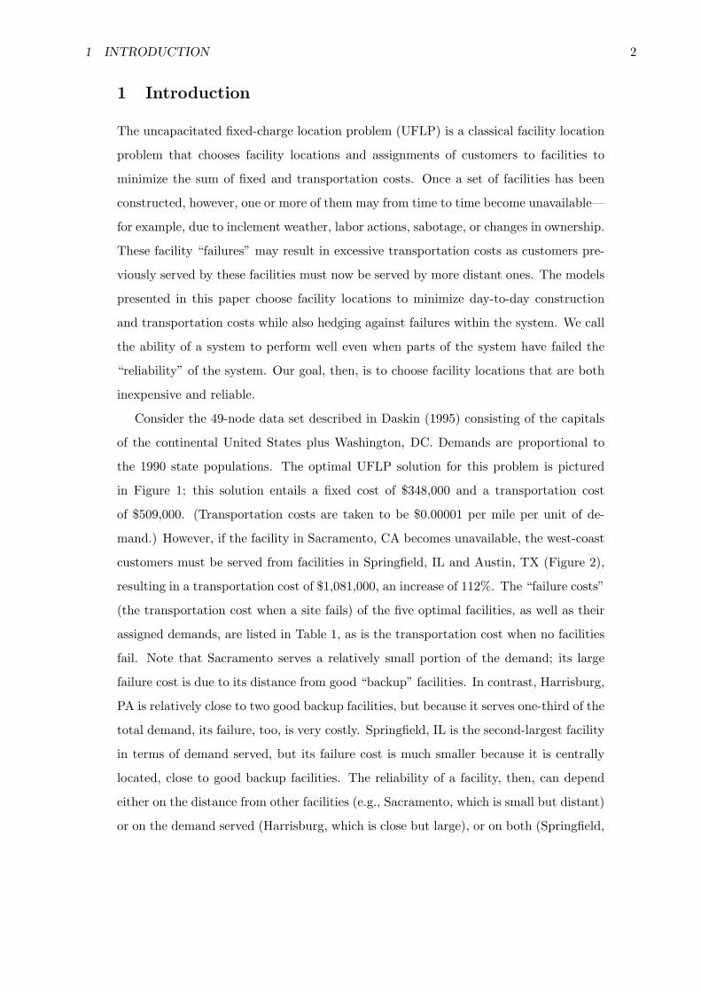
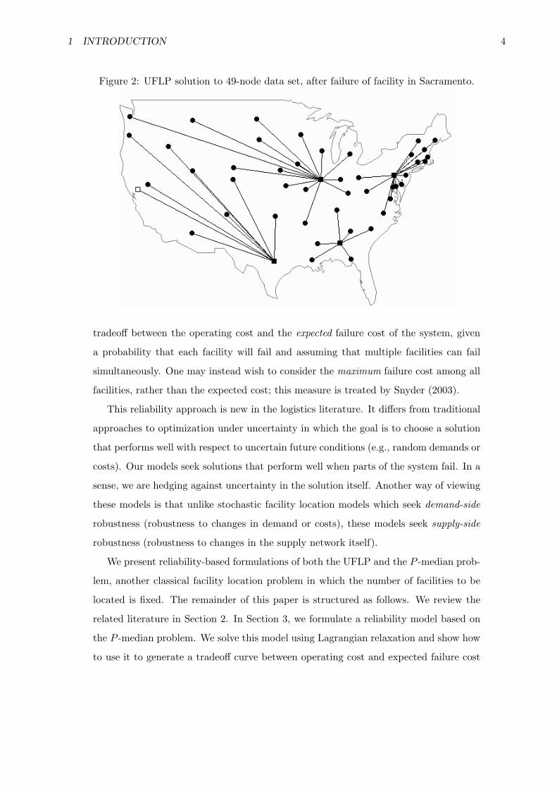
mand.) However, if the facility in Sacramento, CA becomes unavailable, the west-coast
customers must be served from facilities in Springfield, IL and Austin, TX (Figure 2),
resulting in a transportation cost of $1,081,000, an increase of 112%. The “failure costs”
(the transportation cost when a site fails) of the five optimal facilities, as well as their
assigned demands, are listed in Table 1, as is the transportation cost when no facilities
fail. Note that Sacramento serves a relatively small portion of the demand; its large
failure cost is due to its distance from good “backup” facilities. In contrast, Harrisburg,
PA is relatively close to two good backup facilities, but because it serves one-third of the
total demand, its failure, too, is very costly. Springfield, IL is the second-largest facility
in terms of demand served, but its failure cost is much smaller because it is centrally
located, close to good backup facilities. The reliability of a facility, then, can depend
either on the distance from other facilities (e.g., Sacramento, which is small but distant)
or on the demand served (Harrisburg, which is close but large), or on both (Springfield,

1 INTRODUCTION 3
Table 1: Failure costs and assigned demands for UFLP solution.
Location % Demand Served Failure Cost % IncreaseSacramento, CA 19% 1,081,229 112%Harrisburg, PA 33% 917,332 80%Springfield, IL 22% 696,947 37%Montgomery, AL 16% 639,631 26%Austin, TX 10% 636,858 25%Transp. cost w/no failures 508,858 0%
which is reliable because it is neither excessively large nor excessively distant).
Figure 1: UFLP solution to 49-node data set.
A more reliable solution locates facilities in the capitals of CA, NY, TX, PA, OH,
AL, OR, and IA; in this solution, no facility has a failure cost of more than $640,000,
rivaling the smallest failure cost in Table 1. On the other hand, three additional facilities
are used in this solution, and these come at a cost. Few firms would be willing to choose
solutions with location and day-to-day transportation costs that are much greater than
optimal just to hedge against occasional and unpredictable disruptions in their supply
network. One of the goals of this paper is to demonstrate that substantial improvements
in reliability can often be obtained without large increases in day-to-day operating
cost—that by taking reliability into account at design time, one can find a near-optimal
UFLP solution that is much more reliable. This is demonstrated by examining the
1 INTRODUCTION 4
Figure 2: UFLP solution to 49-node data set, after failure of facility in Sacramento.
tradeoff between the operating cost and the expected failure cost of the system, given
a probability that each facility will fail and assuming that multiple facilities can fail
simultaneously. One may instead wish to consider the maximum failure cost among all
facilities, rather than the expected cost; this measure is treated by Snyder (2003).
This reliability approach is new in the logistics literature. It differs from traditional
approaches to optimization under uncertainty in which the goal is to choose a solution
that performs well with respect to uncertain future conditions (e.g., random demands or
costs). Our models seek solutions that perform well when parts of the system fail. In a
sense, we are hedging against uncertainty in the solution itself. Another way of viewing
these models is that unlike stochastic facility location models which seek demand-side
robustness (robustness to changes in demand or costs), these models seek supply-side
robustness (robustness to changes in the supply network itself).
We present reliability-based formulations of both the UFLP and the P -median prob-
lem, another classical facility location problem in which the number of facilities to be
located is fixed. The remainder of this paper is structured as follows. We review the
related literature in Section 2. In Section 3, we formulate a reliability model based on
the P -median problem. We solve this model using Lagrangian relaxation and show how
to use it to generate a tradeoff curve between operating cost and expected failure cost
2 LITERATURE REVIEW 5
using the weighting method of multi-objective programming. In Section 4, we extend
this model to solve a reliability version of the UFLP and discuss a modification that
results in much better computational bounds with little loss of accuracy. We present
computational results in Section 5 and a summary in Section 6.
2 Literature Review
There are three main bodies of literature that are similar in spirit, if not in modeling
approach, to the research presented in this paper. The first is the literature on network
reliability, most often applied to telecommunications or power transmission networks.
The second concerns expected or backup covering models, which are frequently used
in locating emergency services facilities or vehicles. Finally, our models can be seen
as an outgrowth of a small body of literature that discusses approaches for handling
disruptions to supply chains. We discuss each of these three research areas next.
The concept of reliability is borrowed from network reliability theory (Colbourn
1987, Shier 1991, Shooman 2002), which is concerned with computing, estimating, or
maximizing the probability that a network (typically a telecommunications or power
network, represented by a graph) remains connected in the face of random failures.
Failures may be due to disruptions, congestion, or blockages. Almost all of the research
on network reliability considers failures only on the edges, but occasional papers con-
sider node failures as well (e.g., Eiselt, Gendreau, and Laporte 1996). The network
reliability literature tends to focus either on computing reliability or on optimizing it;
i.e., either determining the reliability of a given system or designing a reliable system
from scratch. Computing the reliability of a given network is a non-trivial problem (see,
e.g., Ball 1979), and various performance measures and techniques for computing them
have been proposed. Because of the complications involved in computing reliability,
reliability optimization models rarely include explicit expressions for the reliability of
the network. Instead, they often attempt to find the minimum-cost network design
with some desired structural property, such as 2-connectivity (Monma and Shallcross
1989, Monma, Munson, and Pulleyblank 1990), k-connectivity (Bienstock, Brickell, and
Monma 1990, Grotschel, Monma, and Stoer 1995), or special ring structures (Fortz and
Labbe 2002). The key difference between network reliability models and the models that

2 LITERATURE REVIEW 6
we present in this paper is that network models are concerned entirely with connectivity.
The only costs considered are those to construct the network, not the transportation
cost after rerouting, which is the primary concern of our reliability models.
Our models are also similar in spirit to the vector-assignment P -median problem
(VAPMP) by Weaver and Church (1985) in that we assign customers to facilities at
multiple levels. In the VAPMP, customers are assumed to be served by multiple facilities
based on preference and availability. For example, a given customer might receive 80% of
its demand from its nearest facility, 15% from its second-nearest, and 5% from its third-
nearest. These percentages are inputs to the model. In our models, the “higher-level”
assignments are only used when the primary facilities fail; there are no pre-specified
fractions of demand served by each facility. A similar model, based on the UFLP, is
presented by Pirkul (1989).
Several papers extend the maximum covering problem (Church and ReVelle 1974) to
handle the randomness inherent in locating emergency services vehicles. The classical
maximum covering problem assumes that a vehicle is always available when a call for
service arrives, but this fails to model the congestion in such systems when multiple
calls are received by a facility with limited resources. Daskin (1982) formulates the
maximum expected covering location model (MEXCLM), which assumes a constant,
system-wide probability that a server is busy when a call is received and maximizes the
total expected coverage; he solves the problem heuristically in Daskin (1983). ReVelle
and Hogan (1989) present the maximum availability location problem (MALP), which
allows the availability probability to vary among service areas, while Ball and Lin (1993)
justify the form of the coverage constraints in MEXCLM and MALP using a system
reliability approach.
Larson (1974, 1975) introduced queuing-based location models that explicitly con-
sider customers waiting for service in congested systems. His “hypercube model” is
useful as a descriptive model, but because of its complexity, researchers have had dif-
ficulty incorporating it into optimization models. Berman, Larson, and Chiu (1985)
incorporate the hypercube idea into a simple optimization model, presenting theoreti-
cal results about the trajectory of the optimal 1-median as the demand rate changes in
a general network.
Daskin, Hogan, and ReVelle (1988) compare various stochastic covering problems in

2 LITERATURE REVIEW 7
which the objective is to locate facilities to maximize expected coverage or the degree
of backup coverage. Berman and Krass (2001) consolidate a wide range of approaches
to facility location in congested systems, presenting a complex model that is illustrative
but can be solved only for special cases. The key differences between the expected and
backup coverage models and our models are (1) the objective function (coverage versus
cost) and (2) the nature of the unavailability of a server (congestion versus failures).
Finally, we view our models as an outgrowth of the small body of literature, mainly
appearing in response to the terrorist attacks on September 11, 2001, calling for tech-
niques for designing and operating supply chains that are resilient to disruptions of all
sorts. Articles appearing in academic journals (Sheffi, 2001), business journals (Martha
and Vratimos, 2002; Simchi-Levi, Snyder, and Watson, 2002; Navas, 2003), and popular
magazines (Lynn, 2002) make compelling arguments that supply chains are particularly
vulnerable to intentional or accidental disruptions and suggest possible approaches for
making them less so, but they do not present any quantitative models. We view the
present work as beginning to fill this void.
To our knowledge, the only analytical models considering failures in a facility loca-
tion or supply chain design context are those of Krass, Berman, and Menezes (2003),
Menezes, Berman, and Krass (2003a, 2003b), and Bundschuh, Klabjan, and Thurston
(2003). The first references assume that customers travel from facility to facility in
search of an operational one (for example, when looking for an ATM); their models
minimize a non-linear objective representing the expected cost incurred by customers
as they travel along these paths. Bundschuh, et al. choose suppliers in an inbound sup-
ply chain so that the resulting systems are “reliable” (have a low probability that any
supplier fails) and/or “robust” (are able to maintain a high level of output even after
suppliers have failed). Note that their definition of reliability is somewhat different from
ours. Reliability is enforced by requiring the probability that all suppliers are opera-
tional to exceed a desired level; this is a multi-echelon version of the model proposed by
Vidal and Goetschalckx (2000). System-wide reliability can be improved by switching
to more reliable suppliers, but not by adding redundant suppliers: increasing the num-
ber of suppliers decreases the reliability of the system since it increases the likelihood
that one or more suppliers will fail. The robustness model allows nodes to keep emer-
gency stock on hand and to obtain extra material from operational suppliers when one

3 THE RELIABILITY P -MEDIAN PROBLEM 8
supplier has failed (though it ignores the additional cost that such procurement would
entail). A joint reliability/robustness model combines the two approaches. The authors
test their models on two moderately sized instances using a standard MIP solver with
run-times of up to one hour. They discuss both qualitative (e.g., shifting supply from
Southeast Asia to North America) and quantitative (e.g., changes to the mean and
standard deviation of output, measured using simulation) empirical differences between
solutions from the different models.
3 The Reliability P -Median Problem
In this section we discuss a P -median-based model that minimizes a weighted sum of
the operating cost (the day-to-day transportation cost when all facilities are operational)
and the expected failure cost (the expected transportation cost, taking into account ran-
dom facility failures). Each facility fails with a given probability, and multiple facilities
may fail simultaneously. Certain facilities may be designated as “non-failable.” In our
work with a major manufacturer of durable goods, the facilities that may fail repre-
sent warehouses owned by independent distributors who occasionally “defect” from the
company or go out of business. The non-failable warehouses are those owned by the
company; these are assumed to remain loyal to the firm and will not fail. In other
applications, the non-failable facilities may represent those located in favorable weather
areas, those served by unions with which the firm has a particularly strong relationship,
or other facilities deemed to have a negligible probability of failure.
3.1 Formulation
Let I be the set of customers, indexed by i, and J the set of potential facility locations,
indexed by j. Let NF be the set of candidate facilities that may not fail (we refer to
these as “non-failable” facilities) and let F be the set of candidate facilities that may
fail (“failable” facilities). Note that NF ∪ F = J . Each customer i ∈ I has a demand
hi. The cost per unit of demand to ship from facility j ∈ J to customer i ∈ I is given by
dij . Associated with each customer i is a cost θi that represents the cost of not serving
the customer, per unit of demand. (θi may be a lost-sales cost, or the cost of serving i
by purchasing product from a competitor on an emergency basis). This cost is incurred

3 THE RELIABILITY P -MEDIAN PROBLEM 9
if all open facilities have failed (and thus no facilities are available to serve customer i),
or if θi is less than the cost of assigning i to any of the existing facilities that have not
failed. To model this, we add an “emergency” facility u that is non-failable (u ∈ NF )
and has transportation cost diu = θi to customer i ∈ I. We force Xu = 1 and replace P
with P + 1. From this point forward, we assume that the emergency facility has been
handled in this way, though for simplicity we continue to formulate the problem as a
P -median, rather than as a (P + 1)-median problem.
Each facility in F has a probability q of failing, which is interpreted as the long-
run fraction of time the facility is non-operational. In some cases, q may be estimated
based on historical data (e.g., for weather-induced failures), while in others q must be
estimated subjectively (e.g., for failures due to defection of third-party distributors).
Our model is most easily interpreted as an infinite-horizon model in which q represents
the fraction of time that a facility has failed. However, if the modeler has in mind
a particular time horizon T , then q may be used to capture probabilistic information
about the timing of the failures. For example, suppose each facility has a 0.1 probability
of failing, and that if it fails, it will fail during periods 1 through 5 with probability 0.3
and in periods 3 through T with probability 0.7. (Note that this means that if a facility
fails, it will surely be inoperable during periods 3, 4, and 5.) Then the expected fraction
of time the facility will be non-operational is given by (0.1×0.3×5+0.1×0.7×(T−2))/T .
The strategy behind our formulation is to assign each customer to a primary facility
that will serve it under normal circumstances, as well as to a set of backup facilities
that serve it when the primary facility has failed. Since multiple failures may occur
simultaneously, each customer needs a first backup facility in case its primary facility
fails, a second backup in case its first backup fails, and so on. However, if a customer
is assigned to a non-failable facility as its nth backup, it does not need any further
backups.
There are two sets of decision variables in the model, location variables (X) and
assignment variables (Y ):

3 THE RELIABILITY P -MEDIAN PROBLEM 10
Xj =
1, if a facility is opened at location j
0, otherwise
Yijr =
1, if demand node i is assigned to facility j as a level-r assignment
0, otherwise
A “level-r” assignment is one for which there are r closer failable facilities that are
open. If r = 0, this is a primary assignment; otherwise, it is a backup assignment. Each
customer i has a level-r assignment for each r = 0, . . . , P − 1, unless i is assigned to a
level-s facility that is non-failable, where s < r. In other words, customer i is assigned
to one facility at level 0, another facility at level 1, and so on until i has been assigned
to all open facilities at some level or i has been assigned to a non-failable facility.
We formulate this problem as a multi-objective problem. The objectives are as
follows:
w1 =∑
i∈I
∑
j∈J
hidijYij0
w2 =∑
i∈I
hi
∑
j∈NF
P−1∑
r=0
dijqrYijr +
∑
j∈F
P−1∑
r=0
dijqr(1− q)Yijr
.
Objective w1 computes the operating cost—the P -median cost of serving customers
from their primary facilities. Objective w2 computes the expected failure cost: each
customer i is served by its level-r facility (call it j) if the r closer facilities have failed
(this occurs with probability qr) and if j itself has not failed (this occurs with probability
1− q if j ∈ F and with probability 1 if j ∈ NF ). Note that by the definition of level-r,
all r closer facilities are failable.
Although we refer to w2 as the “expected failure cost,” we are careful to point out
that w2 also includes the transportation cost when no facilities have failed (i.e., the
level-0 assignments). Certainly, there are ways to define reliability other than that
given in w2. For example, if the desired tradeoff is between PMP cost and expected
transportation cost only after a failure, then the “primary” transportation cost can be
omitted from w2 by starting the summation indices at r = 1 rather than r = 0. It is also
possible that the transportation costs for backup assignments are different from those
for primary assignments because, for example, they are arranged with freight companies

3 THE RELIABILITY P -MEDIAN PROBLEM 11
on an emergency basis; in this case, the coefficients for Yijr would be changed from dij
to some other cost for r > 0. Either of these modifications can be handled easily using
the solution method described below.
Our model minimizes a weighted sum αw1 + (1− α)w2 of the two objectives, where
0 ≤ α ≤ 1. By solving the problem for various values of α, one can generate a tradeoff
curve between the operating cost and the expected failure cost using the weighting
method of multi-objective programming (see Section 3.3). The decision maker can
then choose a solution from the tradeoff curve in accordance with his or her preference
between the two objectives. Furthermore, the tradeoff curve can indicate the degree to
which one objective must be sacrificed to improve the other. In our empirical results,
we show that the tradeoff curve for the RPMP is “steep”—that large reductions in
objective w2 can be attained with only small increases in w1.
The reliability P -median problem is formulated as follows:
(RPMP) minimize αw1 + (1− α)w2 (1)
subject to∑
j∈J
Yijr +∑
j∈NF
r−1∑s=0
Yijs = 1 ∀i ∈ I, r = 0, . . . , P − 1 (2)
Yijr ≤ Xj ∀i ∈ I, j ∈ J, r = 0, . . . , P − 1 (3)∑
j∈J
Xj = P (4)
P−1∑r=0
Yijr ≤ 1 ∀i ∈ I, j ∈ J (5)
Xu = 1 (6)
Xj ∈ {0, 1} ∀j ∈ J (7)
Yijr ∈ {0, 1} ∀i ∈ I, j ∈ J, r = 0, . . . , P − 1 (8)
The objective function (1) is straightforward. Constraints (2) require that for each
customer i and each level r, either i is assigned to a level-r facility or it is assigned to
a level-s facility (s < r) that is non-failable. (By convention we take∑r−1
s=0 Yijs = 0 if
r = 0.) Constraints (3) prohibit an assignment to a facility that has not been opened.
Constraint (4) requires P facilities to be opened. Constraints (5) prohibit a customer
from being assigned to a given facility at more than one level. Constraint (6) requires
the emergency facility u to be opened. Constraints (7) and (8) are standard integrality
constraints. (In fact, it is sufficient to require Yijr ≥ 0 in place of (8). We use integrality

3 THE RELIABILITY P -MEDIAN PROBLEM 12
constraints to emphasize the binary nature of the assignment decision; doing so does
not affect our solution procedure.)
For notational convenience, we can write the objective function as
∑
i∈I
∑
j∈J
P−1∑
r=0
ψijrYijr, (9)
where
ψijr =
αhidij + (1− α)hidij = hidij , if r = 0 and j ∈ NF
αhidij + (1− α)hidij(1− q), if r = 0 and j ∈ F
(1− α)hidijqr, if r > 0 and j ∈ NF
(1− α)hidijqr(1− q), if r > 0 and j ∈ F
One might suspect that for small α, the weight on the backup assignments may
be larger than that on the primary assignments, in which case it may be optimal to
assign customers to primary facilities that are farther than their backup facilities, a
situation we would want to prohibit. The next theorem, however, demonstrates that
such a situation cannot occur.
Theorem 1 In any optimal solution to (RPMP), if Yijr = Yik,r+1 = 1 for i ∈ I,
j, k ∈ J , 0 ≤ r < P − 1, then dij ≤ dik.
Proof. Suppose, for a contradiction, that (X,Y ) is an optimal solution to (RPMP) in
which Yijr = Yik,r+1 = 1 but dij > dik. We will show that by “swapping” j and k, the
objective function will decrease. Since i has a level-(r+1) facility (k), its level-r facility
(j) must be failable.
Suppose first that k ∈ F . These two assignments contribute ψijr + ψik,r+1 to the
objective function. If we assigned i to j at level r + 1 and to k at level r, the objective
function would change by (ψikr + ψij,r+1)− (ψijr + ψik,r+1). If r = 0, then
(ψikr + ψij,r+1)− (ψijr + ψik,r+1) =αhidik + (1− α)hidik(1− q) + (1− α)hidijq(1− q)
− αhidij − (1− α)hidij(1− q)− (1− α)hidikq(1− q)
=αhi(dik − dij) + (1− α)hi(dik − dij)(1− q)2
<0

3 THE RELIABILITY P -MEDIAN PROBLEM 13
since dij > dik and 0 ≤ α ≤ 1. On the other hand, if r > 0, then
(ψikr + ψij,r+1)− (ψijr + ψik,r+1) =(1− α)hidikqr(1− q) + (1− α)hidijq
r+1(1− q)
− (1− α)hidijqr(1− q)− (1− α)hidikq
r+1(1− q)
=(1− α)hi(dik − dij)qr(1− q)2
<0.
Either way, the objective function is smaller for the revised solution. The case in which
k ∈ NF is similar, except that in this case, Yij,r+1 = 0 since i’s level-r facility is non-
failable, resulting in an even larger decrease in cost. This contradicts the assumption
that (X, Y ) is optimal.
We note briefly that if the level-0 assignments are excluded from w2 as discussed on
page 10, then Theorem 1 holds when α ≥ 12 , which is generally the range of interest to
decision makers. In this case, the algorithm given below may still be valid for particular
instances, even if α < 12 . If the algorithm returns a solution for which the distance
ordering is obeyed, it is optimal; but the algorithm cannot enforce the distance ordering
if it is not naturally optimal to do so.
3.2 Lagrangian Relaxation
3.2.1 Lower Bound
(RPMP) could be solved using an off-the-shelf IP solver, but in general such an ap-
proach will yield excessive run times, even for moderately sized problems. (See Section
5.3.) This motivates the development of a Lagrangian relaxation algorithm. Relaxing
constraints (2) with Lagrange multipliers λ yields the following Lagrangian subproblem:

3 THE RELIABILITY P -MEDIAN PROBLEM 14
(RPMP-LRλ)
minimize z(λ) =∑
i∈I
∑
j∈J
P−1∑r=0
ψijrYijr +∑
i∈I
P−1∑r=0
λir
1−
∑
j∈J
Yijr −∑
j∈NF
r−1∑s=0
Yijs
(10)
subject to Yijr ≤ Xj ∀i ∈ I, j ∈ J, r = 0, . . . , P − 1 (11)∑
j∈J
Xj = P (12)
P−1∑r=0
Yijr ≤ 1 ∀i ∈ I, j ∈ J (13)
Xu = 1 (14)
Xj ∈ {0, 1} ∀j ∈ J (15)
Yijr ∈ {0, 1} ∀i ∈ I, j ∈ J, r = 0, . . . , P − 1 (16)
The objective function (10) can be re-written as follows:
∑
i∈I
∑
j∈J
P−1∑
r=0
ψijrYijr +∑
i∈I
P−1∑
r=0
λir −∑
i∈I
∑
j∈J
P−1∑
r=0
λirYijr −∑
i∈I
P−1∑
r=0
∑
j∈NF
r−1∑
s=0
λirYijs
=∑
i∈I
∑
j∈J
P−1∑
r=0
ψijrYijr +∑
i∈I
P−1∑
r=0
λir −∑
i∈I
∑
j∈J
P−1∑
r=0
λirYijr −∑
i∈I
∑
j∈NF
P−1∑
s=0
s−1∑
r=0
λisYijr
(by swapping the indices r and s in the last term)
=∑
i∈I
∑
j∈J
P−1∑
r=0
ψijrYijr +∑
i∈I
P−1∑
r=0
λir −∑
i∈I
∑
j∈J
P−1∑
r=0
λirYijr −∑
i∈I
∑
j∈NF
∑r=0,...,P−1s=0,...,P−1
r<s
λisYijr
=∑
i∈I
∑
j∈J
P−1∑
r=0
ψijrYijr +∑
i∈I
P−1∑
r=0
λir −∑
i∈I
∑
j∈J
P−1∑
r=0
λirYijr −∑
i∈I
∑
j∈NF
P−1∑
r=0
(P−1∑
s=r+1
λis
)Yijr
Therefore, the objective function can be written as
∑
i∈I
∑
j∈J
P−1∑
r=0
ψijrYijr +∑
i∈I
P−1∑
r=0
λir, (17)
where
ψijr =
ψijr − λir, if j ∈ F
ψijr − λir −(∑P−1
s=r+1 λis
)= ψijr −
∑P−1s=r λis, if j ∈ NF
(18)

3 THE RELIABILITY P -MEDIAN PROBLEM 15
For given λ, problem (RPMP-LRλ) can be solved easily. Since the assignment con-
straints (2) have been relaxed, customer i may be assigned to zero, one, or more than
one open facility at each level, but it may not be assigned to a given facility at more
than one level r. Suppose that facility j is opened. Customer i will be assigned to
facility j at level r if ψijr < 0 and ψijr ≤ ψijs for all s = 0, . . . , P − 1. Therefore,
the benefit of opening facility j (i.e., the contribution to the objective function if j is
opened) is given by
γj =∑
i∈I
min{
0, minr=0,...,P−1
{ψijr}}
. (19)
Once the benefits γj have been computed for all j, we set Xj = 1 for the emergency
facility u and for the P − 1 remaining facilities with the smallest γj ; we set Yijr = 1 if
(1) facility j is open, (2) ψijr < 0, and (3) r minimizes ψijs for s = 0, . . . , P − 1. The
optimal objective value for (RPMP-LRλ) is z(λ) =∑
j∈J γjXj +∑
i∈I
∑P−1r=0 λir, and
this provides a lower bound on the optimal objective value of (RPMP).
The benefit γj can be computed for a single j in O(nP ) time, where n = |I|, so
all of the benefits can be computed in O(mnP ) time, where m = |J |. Determining
Xj requires sorting the facilities, which takes O(m log m) time, and determining Yijr
requires O(nP ) time, assuming that assignments are stored as a single index j for each
i, r rather than as a list of m 0/1 variables. Therefore, the Lagrangian subproblem can
be solved for a given λ in O(mnP + m log m + nP ) = O(mnP ) time.
3.2.2 Upper Bound
At each iteration of the Lagrangian process, we obtain both a lower and an upper bound.
The solution to (RPMP-LRλ) provides a lower bound. If it is feasible for (RPMP),
then it provides an upper bound as well, and is in fact optimal for (RPMP): since the
constraint violations in (10) equal 0, the lower and upper bounds are equal. If the
solution to (RPMP-LRλ) is not feasible for (RPMP), as is the case in most iterations,
then we construct a feasible solution by opening the facilities that are open in the
solution to (RPMP-LRλ) and assigning customers to the open facilities level by level
in increasing order of distance, until a non-failable facility is assigned. (By Theorem 1,
this is an optimal strategy for assigning customers to a given set of facilities, though the
facilities themselves may not be optimal.) Anecdotally, we can report that the heuristic
3 THE RELIABILITY P -MEDIAN PROBLEM 16
as described here has performed well in our computational tests, finding the optimal
solution very quickly (generally within the first 100 Lagrangian iterations), though we
have not explicitly recorded the iteration at which the optimal solution is found.
3.2.3 Multiplier Updating
Each value of λ provides a lower bound z(λ) on the optimal objective value of (RPMP).
To find the best possible lower bound, we need to solve
maximizeλ∈RnP
z(λ). (20)
This problem is solved approximately using subgradient optimization, applied in a
straightforward manner as described by Fisher (1981, 1985) and Daskin (1995). In
particular, at each iteration n we compute a step-size tn as
tn =βn(UB− Ln)
∑i∈I
P−1∑r=0
(1− ∑
j∈J
Yijr −∑
j∈NF
r−1∑s=0
Yijs
)2 , (21)
where βn is a constant at iteration n, initialized to 2 and halved when 30 consecutive
iterations fail to improve the lower bound; Ln is the value of z(λ) found at iteration n;
and UB is the best known upper bound. The multipliers are updated by setting
λn+1ir ← λn
ir + tn
1−
∑
j∈J
Yijr −∑
j∈NF
r−1∑
s=0
Yijs
. (22)
The Lagrangian process terminates when any of the following criteria are met:
• (UB− Ln)/Ln < ε, for some optimality tolerance ε specified by the user
• n > nmax, for some iteration limit nmax
• βn < βmin, for some β limit βmin
3.2.4 Initial Multipliers
Our algorithm, like many Lagrangian relaxation algorithms, is somewhat sensitive to
the choice of the initial Lagrange multipliers. To develop a strategy for computing good
starting multipliers, we first examined the final multipliers for problems that had been
solved to optimality. We discovered that the final multipliers for k = 0 were roughly on
the order of magnitude of 0.01 times the demand-weighted distance from each customer

3 THE RELIABILITY P -MEDIAN PROBLEM 17
to its assigned facility, and that the optimal multipliers decreased roughly by an order
of magnitude as k increased. Therefore, we settled on the following formula for the
initial multipliers:
λir = hid/10r+2,
where d =∑
i∈I
∑j∈J dij/|I||J | is the average distance between pairs of customers and
facilities.
3.2.5 Branch and Bound
If the Lagrangian process terminates with the lower and upper bounds equal (to within
ε), an ε-optimal solution has been found and the algorithm terminates. Otherwise, we
use branch-and-bound to close the optimality gap. We branch on the Xj (location)
variables. At each branch-and-bound node, the facility selected for branching is the
unfixed open facility with the greatest assigned demand. Xj is first forced to 0 and
then to 1. Branching is done in a depth-first manner. The tree is fathomed at a given
node if the lower bound at that node is within ε of the objective function value of the
best feasible solution found anywhere in the tree, if P facilities have been forced open,
or if |J |−P facilities have been forced closed. The final Lagrange multipliers at a given
node are passed to its child nodes and are used as initial multipliers at those nodes.
3.2.6 Variable Fixing
Suppose that the Lagrangian procedure terminates at the root node of the branch-
and-bound tree with the lower bound strictly less than the upper bound. Assume for
notational convenience that the facilities in J \ {u} are sorted in increasing order of
benefit so that γj ≤ γj+1, under a particular set of Lagrange multipliers λ. Let LB
be the lower bound (the objective value of (RPMP-LRλ)) under the same λ, and let
UB be the best upper bound found. Suppose further that Xj = 0 in the solution to
(RPMP-LRλ). If
LB + γj − γP−1 > UB (23)
then candidate site j cannot be part of the optimal solution, so we can fix Xj = 0.
This is true because if j were forced into the solution, another facility would be forced
out; this facility would be the open facility (other than u) with the largest benefit, i.e.,

3 THE RELIABILITY P -MEDIAN PROBLEM 18
facility P − 1. Clearly LB + γj − γP−1 is a valid lower bound for the “Xj = 1” node (it
would be the first lower bound found if we use λ as the initial multipliers at the new
child node), so we would fathom the tree at this new node and never again consider
setting Xj = 1.
Similarly, suppose Xj = 1 in the solution to (RPMP-LRλ). If
LB− γj + γP > UB (24)
then candidate site j must be part of the optimal solution since swapping j out and
the best closed facility in will result in a solution whose lower bound exceeds the upper
bound; therefore, we can fix Xj = 1.
We perform these variable-fixing checks twice after processing has terminated at
the root node, once using the optimal multipliers λ and once using the most recent
multipliers. This procedure is quite effective in forcing variables open or closed because
the Lagrangian procedure tends to produce tight lower bounds, making (23) or (24)
hold for many facilities j. The time required to perform these checks is negligible.
Variable-fixing tends not to result in substantial improvements if performed at lower
levels of the branch-and-bound tree, so we perform the procedure only at the root node.
3.3 Tradeoff Curve
By systematically varying the objective function weight α and re-solving (RPMP) for
each value, one can generate a tradeoff curve between the two objectives using the
weighting method of multi-objective programming (Cohon 1978). The method is as
follows:
0. Solve (RPMP) for α = 1 (the pure PMP problem) and for α = 0. Add both points
to the tradeoff curve.
1. Identify a pair of adjacent solutions on the tradeoff curve that has not yet been
considered. Let the objective values of these two solutions be (w11, w
12) and (w2
1, w22).
Set α ← −(w12 − w2
2)/(w11 − w2
1 − w12 + w2
2).
2. Solve (RPMP) for the current value of α. If the resulting solution is not already
on the tradeoff curve, add it.
3. If all pairs of adjacent solutions on the tradeoff curve have been explored, stop.
Else, go to 1.

4 THE RELIABILITY FIXED-CHARGE LOCATION PROBLEM 19
4 The Reliability Fixed-Charge Location Problem
The RPMP can improve reliability only by choosing a different set of P facilities, not
by opening additional ones. In this section, we formulate the Reliability Fixed-Charge
Location Problem (RFLP), which is based on the UFLP. Since the UFLP does not
contain a limit on the number of facilities that can be built, the RFLP adds an additional
degree of freedom for improving reliability, namely, constructing additional facilities.
4.1 Formulation
The RFLP is formulated in a manner similar to the RPMP. We need one additional
parameter: fj is the fixed cost to construct a facility at location j ∈ J , amortized to the
time units used to express demands. Since the number of facilities is not known a priori
as it is in the RPMP, we must create assignment variables for levels r = 0, ..., m − 1,
where m ≡ |J |. The objectives are given by
w1 =∑
j∈J
fjXj +∑
i∈I
∑
j∈J
hidijYij0
w2 =∑
i∈I
hi
∑
j∈NF
m−1∑
r=0
dijqrYijr +
∑
j∈F
m−1∑
r=0
dijqr(1− q)Yijr
The emergency facility u is handled as in the RPMP, described in Section 3.1; it has no
fixed cost (fu = 0).
The RFLP is formulated as follows:
(RFLP)
minimize αw1 + (1− α)w2 (25)
subject to∑
j∈J
Yijr +∑
j∈NF
r−1∑s=0
Yijs = 1 ∀i ∈ I, r = 0, . . . , m− 1 (26)
Yijr ≤ Xj ∀i ∈ I, j ∈ J, r = 0, . . . , m− 1 (27)m−1∑r=0
Yijr ≤ 1 ∀i ∈ I, j ∈ J (28)
Xu = 1 (29)
Xj ∈ {0, 1} ∀j ∈ J (30)
Yijr ∈ {0, 1} ∀i ∈ I, j ∈ J, r = 0, . . . , m− 1 (31)
The formulation is identical to that of (RPMP) except:
4 THE RELIABILITY FIXED-CHARGE LOCATION PROBLEM 20
• Fixed costs are included in objective w1
• Constraint (4) is omitted
• The “level” index r is extended to m − 1 instead of P − 1 in summations and
constraint indices
Constraint (29) is not strictly necessary since facility u has 0 fixed cost, but including
the constraint in the formulation tightens the Lagrangian relaxation. As in (RPMP),
contstraints (31) could be relaxed to Yijr ≥ 0. Note that Theorem 1 applies to the
RFLP as well.
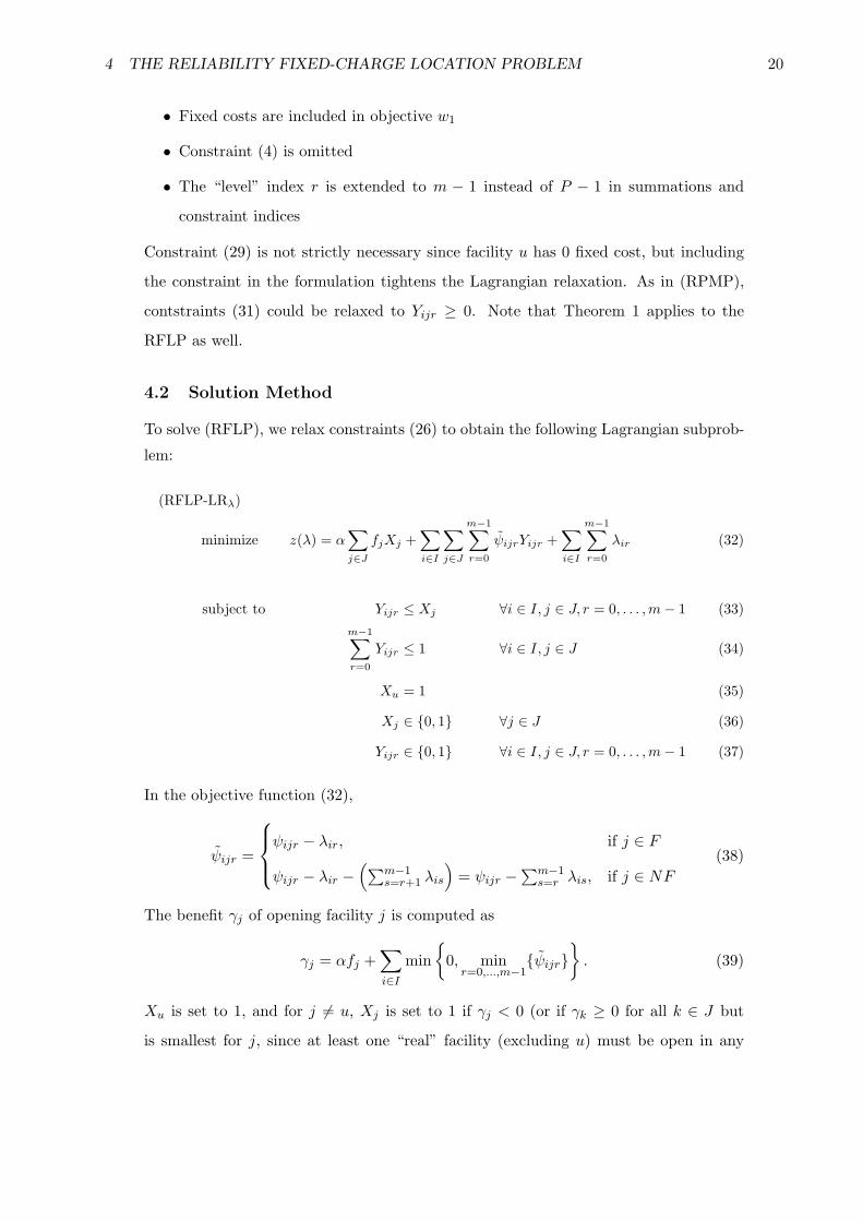
4.2 Solution Method
To solve (RFLP), we relax constraints (26) to obtain the following Lagrangian subprob-
lem:
(RFLP-LRλ)
minimize z(λ) = α∑
j∈J
fjXj +∑
i∈I
∑
j∈J
m−1∑r=0
ψijrYijr +∑
i∈I
m−1∑r=0
λir (32)
subject to Yijr ≤ Xj ∀i ∈ I, j ∈ J, r = 0, . . . ,m− 1 (33)m−1∑r=0
Yijr ≤ 1 ∀i ∈ I, j ∈ J (34)
Xu = 1 (35)
Xj ∈ {0, 1} ∀j ∈ J (36)
Yijr ∈ {0, 1} ∀i ∈ I, j ∈ J, r = 0, . . . ,m− 1 (37)
In the objective function (32),
ψijr =
ψijr − λir, if j ∈ F
ψijr − λir −(∑m−1
s=r+1 λis
)= ψijr −
∑m−1s=r λis, if j ∈ NF
(38)
The benefit γj of opening facility j is computed as
γj = αfj +∑
i∈I
min{
0, minr=0,...,m−1
{ψijr}}
. (39)
Xu is set to 1, and for j 6= u, Xj is set to 1 if γj < 0 (or if γk ≥ 0 for all k ∈ J but
is smallest for j, since at least one “real” facility (excluding u) must be open in any

4 THE RELIABILITY FIXED-CHARGE LOCATION PROBLEM 21
feasible solution to the problem); Yijr is set following the criteria described in Section
3.2.1.
At each Lagrangian iteration, we find an upper bound by opening the facilities that
are open in the solution to (RFLP-LRλ) and greedily assigning customers to them. In
addition, we perform an “add” and a “drop” heuristic on each solution whose objective
value is less than 1.2×UB, where UB is the best known upper bound. The add (drop)
heuristic considers opening (closing) facilities if doing so decreases the objective value.
Each heuristic is performed until no further adds or drops will improve the solution.
The subgradient optimization and branch-and-bound procedures are exactly as de-
scribed for the RPMP, except that branch-and-bound nodes are fathomed if the lower
bound at that node is within ε of the best known upper bound, if |J | (rather than P )
facilities have been forced open, or if |J | − 1 (rather than |J | − P ) facilities have been
forced closed.
4.3 A Modification
In our preliminary computational testing, we found that the subgradient optimization
procedure had difficultly converging to a tight lower bound for the RFLP. We believe
the problem results from the large number of multipliers that must be updated (nm
of them, as opposed to nP in the RPMP). To counteract this effect, we propose the
following modification of our model and algorithm. Since the probability of many facil-
ities failing simultaneously is small, ignoring the simultaneous failure of more than, say,
5 facilities may result in a very small loss of accuracy. At the same time, the reduction
in the number of multipliers may result in a very large improvement in computational
performance. Customers would only be assigned to facilities at levels 0 through 4, and
higher-level assignments would not be included either in the objective function or in
the constraints. In fact, if we interpret m as the number of levels to be assigned, rather
than as the cardinality of J , then the objective functions w1 and w2 and the formula-
tion of (RFLP) remain intact under this new modeling scheme, as does the Lagrangian
relaxation (RFLP-LRλ) and the algorithm for solving it. The emergency facility may
become irrelevant in this case, since it is generally used only when all open facilities
have failed, but it may still play a role in the solution if the emergency cost is smaller
than the cost of serving a given customer from, say, its fourth nearest facility when the

5 COMPUTATIONAL RESULTS 22
first three have failed.
We observed similar convergence problems in the RPMP when P was large. The
same modification may be made to (RPMP) by replacing P with m (except in constraint
(4)). We have found this modification to be very effective for both problems; our
computational experience with this modification is presented in Section 5.5.
5 Computational Results
5.1 Experimental Design
We tested our algorithms on five data sets with up to 150 nodes.1 The first three
(see Daskin 1995) are derived from 1990 census data: a 49-node set consisting of the
state capitals of the continental United States plus Washington, DC; an 88-node set
consisting of the 49-node set plus the 50 largest cities in the U.S., minus duplicates; and
a 150-node set consisting of the 150 largest cities in the U.S. Demands hi are set to the
state population divided by 105 for the 49-node set and to the city population divided
by 104 for the other two. The fixed cost fj is set to the median home value in the city
for the 49- and 88-node sets and to 105 for all j in the 150-node set. The transportation
cost dij is set equal to the great-circle distance between i and j. The emergency cost θi
is set to 104 for all i.
The remaining two data sets were generated randomly. One data set consists of
50 nodes, the other consists of 100 nodes. In both cases, demands hi were drawn
from U [0, 1000] and rounded to the nearest integer, fixed costs fj were drawn from
U [500, 1500] and rounded to the nearest integer, and x and y coordinates were drawn
from U [0, 1]. Transportation costs dij are set equal to the Euclidean distance between
i and j. The emergency cost θi is set to 10 to model the situation in which losing a
customer is extremely costly.
In all five data sets, the set I of customers and the set J of facilities are equal
(i.e., every customer may become a DC). q was set to 0.05. We tested the RPMP
algorithm for P = 5, 10, and 20, as well as the RFLP algorithm, using six different
values of α. (We did not use the weighting method described in Section 3.3 in these
initial tests; see Section 5.4 for results using the weighting method.) We executed the1All data sets may be obtained from the lead author’s web site.
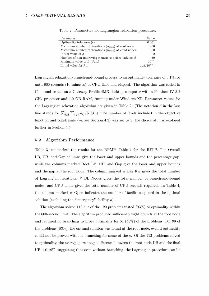
5 COMPUTATIONAL RESULTS 23
Table 2: Parameters for Lagrangian relaxation procedure.
Parameter Value
Optimality tolerance (ε) 0.001Maximum number of iterations (nmax) at root node 1200Maximum number of iterations (nmax) at child nodes 600Initial value of β 2Number of non-improving iterations before halving β 30Minimum value of β (βmin) 10−8
Initial value for λis µid/10k+2
Lagrangian relaxation/branch-and-bound process to an optimality tolerance of 0.1%, or
until 600 seconds (10 minutes) of CPU time had elapsed. The algorithm was coded in
C++ and tested on a Gateway Profile 4MX desktop computer with a Pentium IV 3.2
GHz processor and 1.0 GB RAM, running under Windows XP. Parameter values for
the Lagrangian relaxation algorithm are given in Table 2. (The notation d in the last
line stands for∑
i∈I
∑j∈J dij/|I||J |.) The number of levels included in the objective
function and constraints (m; see Section 4.3) was set to 5; the choice of m is explored
further in Section 5.5.
5.2 Algorithm Performance
Table 3 summarizes the results for the RPMP, Table 4 for the RFLP. The Overall
LB, UB, and Gap columns give the lower and upper bounds and the percentage gap,
while the columns marked Root LB, UB, and Gap give the lower and upper bounds
and the gap at the root node. The column marked # Lag Iter gives the total number
of Lagrangian iterations, # BB Nodes gives the total number of branch-and-bound
nodes, and CPU Time gives the total number of CPU seconds required. In Table 4,
the column marked # Open indicates the number of facilities opened in the optimal
solution (excluding the “emergency” facility u).
The algorithm solved 112 out of the 120 problems tested (93%) to optimality within
the 600-second limit. The algorithm produced sufficiently tight bounds at the root node
and required no branching to prove optimality for 51 (43%) of the problems. For 99 of
the problems (83%), the optimal solution was found at the root node, even if optimality
could not be proved without branching for some of these. Of the 112 problems solved
to optimality, the average percentage difference between the root-node UB and the final
UB is 0.19%, suggesting that even without branching, the Lagrangian procedure can be

5 COMPUTATIONAL RESULTS 24
Table 3: Algorithm results: RPMP.
Overall Overall Overall Root Root Root # Lag # BB CPUNodes P α LB UB Gap LB UB Gap Iter Nodes Time
49 5 1.0 502233 502732 0.10% 502233 502732 0.10% 893 1 3.649 5 0.8 517694 518210 0.10% 517694 518210 0.10% 149 1 0.749 5 0.6 533158 533687 0.10% 533158 533687 0.10% 175 1 0.849 5 0.4 547760 548279 0.09% 547760 548279 0.09% 308 1 1.349 5 0.2 561877 562437 0.10% 561877 562437 0.10% 139 1 0.649 5 0.0 575577 576153 0.10% 575577 576153 0.10% 87 1 0.4
49 10 1.0 275430 275701 0.10% 274143 275701 0.57% 2557 7 10.849 10 0.8 283320 283601 0.10% 283320 283601 0.10% 592 1 2.549 10 0.6 291215 291501 0.10% 291215 291501 0.10% 471 1 2.049 10 0.4 299109 299402 0.10% 299109 299402 0.10% 776 1 3.249 10 0.2 306996 307302 0.10% 306996 307302 0.10% 416 1 1.749 10 0.0 314889 315202 0.10% 314889 315202 0.10% 334 1 1.4
49 20 1.0 113225 113330 0.09% 82862 113852 37.40% 31018 87 139.649 20 0.8 119543 119663 0.10% 106923 122780 14.83% 11183 27 51.649 20 0.6 125870 125995 0.10% 120449 128150 6.39% 15099 37 70.249 20 0.4 132203 132328 0.09% 128782 133784 3.88% 5454 15 24.849 20 0.2 138523 138661 0.10% 127997 138704 8.37% 8170 19 37.249 20 0.0 144783 144926 0.10% 140842 145767 3.50% 8450 21 39.3
88 5 1.0 873996 874859 0.10% 873996 874859 0.10% 436 1 4.788 5 0.8 900827 901706 0.10% 900827 901706 0.10% 389 1 4.288 5 0.6 927662 928554 0.10% 927662 928554 0.10% 103 1 1.388 5 0.4 954455 955402 0.10% 954455 955402 0.10% 198 1 2.288 5 0.2 981308 982249 0.10% 981308 982249 0.10% 269 1 3.088 5 0.0 1003250 1004250 0.10% 1003250 1004250 0.10% 122 1 1.5
88 10 1.0 511663 512174 0.10% 508454 512174 0.73% 4232 11 45.188 10 0.8 525170 525694 0.10% 524923 525694 0.15% 1349 3 13.088 10 0.6 538678 539215 0.10% 538376 539215 0.16% 1279 3 12.788 10 0.4 552186 552735 0.10% 552186 552735 0.10% 286 1 2.988 10 0.2 565700 566256 0.10% 565700 566256 0.10% 839 1 8.088 10 0.0 579190 579761 0.10% 579137 579761 0.11% 1369 3 13.5
88 20 1.0 233427 250125 7.15% 176156 263303 49.47% 55552 132 > 600.088 20 0.8 259784 260039 0.10% 254057 271712 6.95% 38714 93 440.488 20 0.6 269685 269953 0.10% 254396 275915 8.46% 7959 17 92.388 20 0.4 279589 279867 0.10% 273182 282220 3.31% 28058 61 340.588 20 0.2 289048 289330 0.10% 279108 290975 4.25% 37680 91 436.688 20 0.0 298422 298720 0.10% 289268 299303 3.47% 13700 29 159.5
150 5 1.0 1196980 1198160 0.10% 1196980 1198160 0.10% 260 1 8.0150 5 0.8 1213000 1214190 0.10% 1213000 1214190 0.10% 364 1 10.8150 5 0.6 1225190 1226190 0.08% 1225190 1226190 0.08% 190 1 6.1150 5 0.4 1231040 1232270 0.10% 1231040 1232270 0.10% 325 1 9.7150 5 0.2 1233870 1234390 0.04% 1233870 1234390 0.04% 312 1 9.4150 5 0.0 1233910 1234390 0.04% 1233910 1234390 0.04% 276 1 8.5
150 10 1.0 738461 739200 0.10% 659817 739200 12.03% 8919 19 250.2150 10 0.8 754318 755072 0.10% 749869 755072 0.69% 8663 19 243.9150 10 0.6 766172 766938 0.10% 762862 769430 0.86% 13438 27 394.1150 10 0.4 771397 772152 0.10% 769677 772152 0.32% 2641 5 77.5150 10 0.2 773701 774243 0.07% 772587 774243 0.21% 2904 5 83.7150 10 0.0 773477 774243 0.10% 773477 774243 0.10% 556 1 14.7
150 20 1.0 137992 380309 175.60% 137992 380309 175.60% 21282 50 > 600.0150 20 0.8 349152 382366 9.51% 349152 386197 10.61% 19074 40 > 600.0150 20 0.6 383377 383749 0.10% 375513 387837 3.28% 9586 21 295.5150 20 0.4 387808 388180 0.10% 387791 388180 0.10% 4301 9 132.9150 20 0.2 391763 392127 0.09% 347132 393858 13.46% 7416 17 208.0150 20 0.0 394907 395299 0.10% 344463 397887 15.51% 9045 19 253.4
(continued on next page)

5 COMPUTATIONAL RESULTS 25
Table 3: Algorithm results: RPMP (cont’d).
Overall Overall Overall Root Root Root # Lag # BB CPUNodes P α LB UB Gap LB UB Gap Iter Nodes Time
50 5 1.0 3209 3212 0.10% 3209 3212 0.10% 982 1 4.250 5 0.8 3261 3264 0.10% 3261 3264 0.10% 501 1 2.250 5 0.6 3312 3316 0.10% 3312 3316 0.10% 640 1 2.850 5 0.4 3364 3367 0.10% 3364 3367 0.10% 494 1 2.250 5 0.2 3409 3413 0.10% 3409 3413 0.10% 416 1 1.850 5 0.0 3455 3458 0.09% 3455 3458 0.09% 279 1 1.2
50 10 1.0 1644 1645 0.09% 723 1645 127.64% 9523 23 44.050 10 0.8 1687 1689 0.10% 1338 1689 26.22% 6007 13 27.350 10 0.6 1730 1732 0.10% 1710 1732 1.28% 2361 5 10.850 10 0.4 1774 1776 0.09% 1774 1776 0.09% 1043 1 4.550 10 0.2 1817 1819 0.10% 1783 1819 2.04% 2533 5 11.450 10 0.0 1861 1863 0.10% 1847 1863 0.85% 1675 3 7.4
50 20 1.0 719 720 0.10% -4852 734 — 36595 97 173.050 20 0.8 745 746 0.10% -1696 746 — 12550 29 58.850 20 0.6 772 773 0.10% -5728 789 — 19179 45 92.150 20 0.4 799 800 0.10% -2124 800 — 17184 41 88.250 20 0.2 825 826 0.10% -54 826 — 14738 33 71.550 20 0.0 852 853 0.10% -2757 853 — 18610 45 88.9
100 5 1.0 8351 8359 0.09% 8324 8359 0.41% 3266 7 41.1100 5 0.8 8466 8474 0.10% 8446 8474 0.33% 2557 5 31.5100 5 0.6 8577 8586 0.10% 8565 8586 0.24% 1414 3 17.3100 5 0.4 8688 8697 0.10% 8683 8697 0.16% 1364 3 16.9100 5 0.2 8800 8808 0.10% 8800 8808 0.10% 346 1 4.5100 5 0.0 8911 8920 0.10% 8911 8920 0.10% 193 1 2.5
100 10 1.0 4858 4863 0.10% 4218 4863 15.28% 6775 17 84.7100 10 0.8 4947 4952 0.10% 4910 4952 0.85% 2124 5 27.0100 10 0.6 5036 5041 0.10% 5025 5041 0.31% 1651 3 20.3100 10 0.4 5125 5130 0.09% 5125 5130 0.09% 570 1 6.9100 10 0.2 5210 5215 0.10% 5143 5215 1.39% 3421 9 45.0100 10 0.0 5289 5294 0.10% 5149 5294 2.80% 3456 7 45.9
100 20 1.0 27 2776 10041.40% 27 2776 10041.40% 45607 102 > 600.0100 20 0.8 2816 2835 0.69% -384 2835 — 42301 97 > 600.0100 20 0.6 461 2895 528.56% 461 2896 528.84% 39946 96 > 600.0100 20 0.4 2947 2950 0.10% 1012 2955 191.88% 38700 91 574.9100 20 0.2 3003 3005 0.07% 718 3005 318.51% 31762 71 413.2100 20 0.0 3056 3059 0.10% 828 3059 269.48% 34386 81 475.5

5 COMPUTATIONAL RESULTS 26
Table 4: Algorithm results: RFLP.
Overall Overall Overall Root Root Root # Lag # BB CPUNodes α LB UB Gap LB UB Gap Iter Nodes Time # Open
49 1.0 855959 856810 0.10% 830504 856810 3.17% 4149 11 19.2 649 0.8 790275 791014 0.09% 790275 791014 0.09% 201 1 1.1 649 0.6 707332 707982 0.09% 707332 707982 0.09% 361 1 1.8 849 0.4 589099 589677 0.10% 589099 589677 0.10% 524 1 3.0 1049 0.2 404512 404903 0.10% 403946 404903 0.24% 1518 3 6.8 1649 0.0 19285 19303 0.09% 18510 19303 4.28% 1956 5 8.1 49
88 1.0 1200700 1201880 0.10% 1200700 1201880 0.10% 394 1 5.1 988 0.8 1112990 1114070 0.10% 1112990 1114070 0.10% 598 1 7.8 988 0.6 1011980 1012970 0.10% 1011980 1012970 0.10% 736 1 9.7 1088 0.4 871495 872364 0.10% 855355 872364 1.99% 13185 31 273.6 1488 0.2 605380 605983 0.10% 603911 605983 0.34% 2959 7 46.0 2488 0.0 17695 17712 0.10% 17278 17712 2.52% 2639 7 27.7 88
150 1.0 1668620 1670290 0.10% 1668620 1670290 0.10% 835 1 26.3 7150 0.8 1546990 1548350 0.09% 1546990 1548350 0.09% 464 1 19.0 8150 0.6 1350270 1351600 0.10% 1350270 1351600 0.10% 865 1 41.8 12150 0.4 1094320 1095400 0.10% 1094320 1095400 0.10% 302 1 13.7 14150 0.2 791337 792127 0.10% 791337 792127 0.10% 546 1 28.6 20150 0.0 11116 11126 0.09% 8615 11126 29.15% 1498 3 43.2 150
50 1.0 6727 6733 0.10% 6727 6733 0.10% 818 1 3.6 450 0.8 6208 6214 0.10% 6208 6214 0.10% 653 1 2.9 550 0.6 5612 5617 0.10% 5612 5617 0.10% 927 1 4.2 550 0.4 4862 4866 0.09% 4844 4866 0.47% 1288 3 6.5 650 0.2 3558 3561 0.10% 1799 3561 97.94% 10876 27 60.3 1150 0.0 81 81 0.10% -10676 81 — 15833 43 70.6 50
100 1.0 11482 11493 0.10% 11067 11493 3.85% 10965 27 169.7 7100 0.8 10623 10633 0.09% 10623 10633 0.09% 522 1 8.6 8100 0.6 9574 9584 0.10% 9387 9584 2.09% 3945 9 62.0 9100 0.4 5025 8333 65.83% 5025 8333 65.83% 22219 50 > 600.0 11100 0.2 3406 6231 82.94% 3406 6231 82.94% 8503 17 > 600.0 17100 0.0 132 133 0.10% -20941 133 — 25671 71 365.7 100

5 COMPUTATIONAL RESULTS 27
relied upon to produce good feasible solutions.
The root-node lower bound was quite weak (sometimes even negative) for some of the
problems. We believe this is due primarily to the choice of the initial Lagrange multipli-
ers, and that with additional experimentation, one could find better starting multipliers
for a given problem. Indeed, the branch-and-bound process generally improved the mul-
tipliers quickly, and all but a few of these problems were solved to optimality within the
600-second limit. For the few problems for which the branch-and-bound process exe-
cuted for the full 600 seconds without improving the bounds, the “right-hand” branch
of the tree was never explored, preventing the overall lower bound from being updated;
nevertheless, improvement was made in the lower bound in the left-hand branch.
Two trends are evident from Tables 3 and 4. First, the algorithm performs worse in
terms of both gap sizes and CPU time when P is large. This is not surprising since these
problems have many more feasible solutions, and finding good Lagrange multipliers can
be particularly difficult. Second, the algorithm often produces weak bounds when α = 1.
This is surprising at first since α = 1 is the “easy” case—the pure PMP (or UFLP)
problem. However, these pure problems have many extraneous variables and constraints;
the extra variables have no bearing on the objective function, leading to a large number
of optimal solutions that are difficult to prove optimal. Location problems with highly
regular cost structures (e.g., many customers are equidistant from many facilities) are
well known to be difficult to solve. Moreover, the poor performance when α = 1 is not
a problem since good algorithms already exist for the classical PMP and UFLP.
Finally, we note that, not surprisingly, the number of facilities opened in optimal
solutions to the RFLP increases as α decreases, since for small α the emphasis is on
reliability more than operational cost. In the extreme case in which α = 0, the fixed
costs are not included in the objective function at all, and the resulting solution is
trivial: all facilities are open.
5.3 CPLEX Performance
To demonstrate the difficulty in solving (RPMP) and (RFLP) using an off-the-shelf IP
solver, we solved an instance of each problem using CPLEX 8.1. We coded (RPMP) and
(RFLP) in AMPL and solved the 50-node Euclidean data set using the same computer
described in Section 5.1. All CPLEX options were set to their default values, except

5 COMPUTATIONAL RESULTS 28
Table 5: CPLEX performance.
LR CPLEX LR CPLEX # Simplex # BBProblem α Time Time Obj Obj Iter Nodes
RPMP (P = 10) 1.0 44.0 4.5 1645 1645 5017 00.8 27.3 > 1800.0 1689 1689 118568 50.6 10.8 > 1800.0 1732 1732 192730 90.4 4.5 > 1800.0 1776 1776 98591 00.2 11.4 > 1800.0 1819 1819 121438 20.0 7.4 > 1800.0 1863 1863 307822 117
RFLP 1.0 3.6 32.2 6733 6734 11487 00.8 2.9 79.0 6214 6214 39009 00.6 4.2 151.5 5617 5618 46791 00.4 6.5 101.1 4866 4867 38104 00.2 60.3 > 1800.0 3561 4079 47498 00.0 70.6 8.0 81 81 2975 0
that we imposed a maximum time limit of 1800 seconds (30 minutes). We tested six
values of α for each problem. P was set to 10 for the (RPMP) instances. The results
are reported in Table 5. The columns labeled LR Time and LR Obj indicate the CPU
time and objective value returned by our Lagrangian relaxation algorithm (reproduced
from Tables 3 and 4), while those labeled CPLEX Time and CPLEX Obj indicate the
corresponding values for CPLEX. The last two columns report the number of simplex
iterations and branch-and-bound nodes as reported by CPLEX.
CPLEX required more time than our Lagrangian algorithm to solve 10 of the 12
problems tested, and for half of the problems, CPLEX could not prove optimality within
the 30-minute limit, although CPLEX did find an optimal or near-optimal solution for
all but one of the problems. CPLEX seemed to have an easier time solving the RFLP
than the RPMP, solving 5 of the 6 RFLP problems without branching. (This is the
result of CPLEX’s pre-processing and cut-generation features; it does not mean that
the LP relaxation has integer optimal solutions. For example, the RFLP with α = 0.6
has an optimal objective value of 5617, while its LP relaxation has an optimal objective
value of 5598.) This discussion suggests that CPLEX is not a reliable tool for solving the
problems at hand, motivating the development of the Lagrangian relaxation algorithm
presented above.
5.4 Tradeoff Curves
We constructed the tradeoff curve for the RFLP using the 49-node data set as described
in Section 3.3; the results are pictured in Figure 3. The horizontal axis plots the UFLP

5 COMPUTATIONAL RESULTS 29
cost (objective 1) while the vertical axis plots the expected failure cost (objective 2).
Each point on the curve represents a different solution; the optimal UFLP solution
(found by solving (RFLP) with α = 1) is the left-most point on the curve. The steep-
ness of the left part of the curve indicates that large improvements in reliability can
be attained without large increases in UFLP cost to improve reliability. The 10 left-
most solutions on the curve are listed in Table 6, along with their relationship to the
UFLP solution and the number of facilities open in the solution. Decision-makers may
be reluctant to undertake large increases in UFLP cost, but they may be willing, for
example, to expend 7% more to reduce expected failure cost by 27%, as in solution 4.
The points at the right of the tradeoff curve are unlikely to be of much interest, as they
represent solutions in which nearly all of the facilities are open; they have extremely
low failure costs but are very expensive to implement. In general, we find that the left
portion of the tradeoff curve is quite steep, indicating that substantial improvements in
reliability can be attained with minimal increases in operational cost.
Figure 3: RFLP tradeoff curve for 49-node data set.
0
100
200
300
400
500
600
500 1000 1500 2000 2500 3000 3500 4000
UFLP Cost (x1000)
Exp
ecte
d F
ailu
re C
ost
(x1
000)
The tradeoff curve in Figure 3 was constructed assuming all facilities are failable.
Firms may be interested in knowing how the tradeoff curve changes if some of the
facilities in J are non-failable. This may help firms make decisions about which contracts
should be shored up or which DCs should be owned in-house, for example. Figure 4

5 COMPUTATIONAL RESULTS 30
Table 6: First 10 solutions in curve: RFLP.
Soln Obj 1 Obj 2 % Increase Obj 1 % Decrease Obj 2 # Locations
1 856810 532199 — — 72 860078 514758 0.4% 3.3% 73 883656 460699 3.1% 13.4% 84 919203 391149 7.3% 26.5% 95 946914 356139 10.5% 33.1% 106 984969 326149 15.0% 38.7% 117 1014350 306754 18.4% 42.4% 128 1062410 275649 24.0% 48.2% 139 1104380 250493 28.9% 52.9% 1410 1151970 226437 34.4% 57.5% 15
contains two tradeoff curves, the one in which all facilities are failable (discussed earlier)
and another in which 25 of the 49 facilities, chosen randomly, are designated as non-
failable. The inclusion of non-failable facilities has the effect of shifting the tradeoff curve
favorably toward the origin. (In addition, problems with more non-failable facilities
generally produce tighter bounds and require less computation time.)
Figure 4: Shifting tradeoff curve.
0
100
200
300
400
500
600
500 1000 1500 2000 2500 3000 3500 4000
UFLP Cost (x1000)
Exp
ecte
d F
ailu
re C
ost
(x
1000
)
All Failable 50% Non-Failable
A natural question to ask is, how many non-failable facilities need to be included
in the set of potential facility sites to achieve a satisfactory level of reliability? Figure
5 addresses this question by plotting the decrease in objective function value as the
number of non-failable facilities increases, using the RFLP and the 49-node data set
with α = 0.8 and q = 0.10. In the lower curve (marked “Last Solution”), the non-
failable facilities were selected from the previous solution. This curve represents how

5 COMPUTATIONAL RESULTS 31
the objective function might change if the firm could make any facilities that it likes
non-failable. In the upper curve (marked “Random”), the non-failable facilities are
chosen randomly. This represents the case in which the firm has no control over which
facilities are non-failable. Note that in both cases, the horizontal axis plots the number
of non-failable facilities that are in J ; not all of these will necessarily be chosen in the
solutions. From the chart it is apparent that only a few non-failable DCs are necessary
to make the solution as a whole substantially more reliable. For our client, the durable
goods manufacturer, this means that the company needs to own only a few DCs in-house
to make the system perform well when third-party distributors fail. It also allows the
firm to threaten to cancel contracts with badly performing distributors, since the firm
can credibly claim to be able to operate without the distributor, at least in the short
term, while they establish a contract with a new distributor. This is an important issue
in contract negotiation and enforcement.
Figure 5: Changing the number of non-failing facilities.
400
420
440
460
480
500
520
540
560
580
600
0 1 2 3 4 5 6 7 8
# of Non-Failable Facilities
Exp
ecte
d F
ailu
re C
ost
(x1
000)
Random Last Solution

6 CONCLUSIONS 32
Table 7: Sensitivity to m.
Problem m Root Gap # Lag Iter # BB Nodes CPU Time Time/Iter
RPMP 3 0.10% 391 1 1.3 0.003RPMP 5 0.10% 592 1 2.7 0.005RPMP 7 0.88% 2018 5 10.9 0.005RPMP 9 1.24% 7185 19 44.4 0.006RPMP 11 1.11% 6445 17 46.7 0.007RFLP 3 0.07% 120 1 0.5 0.005RFLP 5 0.09% 201 1 1.1 0.006RFLP 8 0.98% 4102 11 31.5 0.008RFLP 12 0.64% 4233 11 41.0 0.010RFLP 20 0.66% 4279 11 57.4 0.013RFLP 50 0.54% 3996 9 102.1 0.026
5.5 Number of Levels
In this section we briefly explore the impact of changing the number of levels, m, as
discussed in Section 4.3. We solved the RPMP with P = 10 and the RFLP using the
88-node data set, α = 0.8, and q = 0.05, testing various values of m. The results
are presented in Table 7. (Note that the last entry for each problem corresponds to
the case in which we do not use the modification suggested in Section 4.3. Since the
emergency facility has been added to the problem, m = 50 for the RFLP and m = 11
for the RPMP since |J | and P increased by 1 when the emergency facility was added.)
The column marked Time/Iter gives the average number of CPU seconds spent on
each Lagrangian iteration. From the table it is apparent that using larger values of m
generally results in larger root-node optimality gaps, more Lagrangian iterations, more
branch-and-bound nodes, and more time spent on each iteration (due to loops of the
form “for r = 0, . . . , m − 1”). It is worth pointing out that in all cases, regardless of
the value of m, the algorithm returned the same set of facility locations (one set for the
RPMP and one for the RFLP), indicating that the computational improvement came
at no loss of solution accuracy, though of course we cannot prove that this will hold in
general.
6 Conclusions
In this paper we presented two new models that incorporate reliability into classical
facility location problems. These models arose from a realization that supply chains are
vulnerable to disruptions of all sorts, and that facility location decisions can be critical

6 CONCLUSIONS 33
in reducing the impact of these disruptions. We formulated reliability models based
on the P -median problem and the uncapacitated fixed-charge location problem, called
the RPMP and RFLP, respectively. Key to our formulation is the concept of “backup”
assignments, which represent the facilities to which customers are assigned when closer
facilities have failed. In both models, the expected transportation cost, taking into
account the costs that result from facility failures, is included in the objective function.
The tradeoff of interest is between the operating cost (the traditional PMP or UFLP
objective function) and the expected failure cost. In a subsequent paper, we will address
the tradeoff between operating cost and the maximum failure cost over all facilities
in the solution. Both models are solved using Lagrangian relaxation, with promising
results. We demonstrated empirically that the interesting portion of the tradeoff curve
is steep, indicating that reliability can be drastically improved without large increases
in operating costs. This is a critical issue for decision-makers who may be reluctant to
expend greater sums for sure in order to hedge against possible failures in the future.
For large values of P in the RPMP, and for the RFLP, straightforward application
of our algorithm yielded large gaps at the root node. We proposed a modification that
entails assigning facilities only to a pre-specified level m (we used m = 5). This mod-
ification tightens these bounds considerably with little or no loss of accuracy. In our
computational tests, we found that the choice of m has a large impact on computational
performance but no impact on the solution found. For different values of m, the ob-
jective function for the solutions differed slightly since higher-level terms are excluded
for smaller values of m. However, we found this difference to be less than 0.02% in all
cases. This addresses an important question about the bounds produced by our algo-
rithm. In particular, when a Lagrangian relaxation algorithm produces lower bounds
that are loose, one always wants to know whether this is the theoretical lower bound
(the maximum value of z(λ) in (20), regardless of whether we can find it in practice) or
simply a practical lower bound (the bound actually produced by a computer implemen-
tation) that might be improved by a different multiplier updating method or different
choices of algorithm parameters. Consider the last entry in Table 7. When we began
testing, we assumed that the theoretical bound for this problem was 0.54% away from
the optimal solution, or close to it. When m = 3, however, we get a lower bound that
is only 0.07% from the upper bound, and since this upper bound is very close (within

6 CONCLUSIONS 34
0.02%, as discussed above) to the upper bound when all assignment levels are included
in the objective function, we can be confident that the theoretical lower bound is no
more than 0.1% from the optimal solution. This suggests that the size of the practical
bounds is to some extent determined by our implementation of the multiplier updating
routine, and not by the theoretical bound, and that we might tighten this bound even
further by improving this routine or by choosing better initial multipliers. (This is es-
pecially important for the larger problems tested, which resulted in bounds significantly
larger than 0.1% at the root node.)
We also note that our upper-bound heuristic and improvement routines are highly
effective, yielding the optimal solution at the root node in 99 of 120 problems tested
(83%), including all of the RFLP problems, often finding it within the first 100 iterations
or so. This suggests that very good solutions can be found very quickly, if a theoretical
guarantee of optimality is not required.
The main drawback of our models is the assumption that failable facilities all have the
same probability q of failing. This assumption is necessary to allow us to compute the
probability that a customer is served by its level-r facility without explicitly knowing
its lower-level assignments, only that there are r of them and that they are failable.
Increasing the number of probabilities results in an exponential increase in the number of
terms in the objective function, since one term is required for each possible combination
of the failure probabilities of the r lower-level assignments. We intend to study this issue
in future research to find an objective function that can accommodate multiple failure
probabilities.
Another limitation of our models is the assumption that the facilities are uncapac-
itated. While this is a common assumption made in facility location models, it may
be unrealistic in practice. In the reliability context, customers of failed facilities can
only be assigned to backup facilities if those facilities have enough excess capacity to
accommodate the additional demand. This makes the capacitated case significant from
a practical perspective; it also makes the capacitated model more complex than capac-
itated versions of classical models. In any case, the capacitated model is another topic
worthy of future study.
Finally, we note that if decision makers are interested only in total expected cost, not
in the tradeoff between the PMP or UFLP objective and the expected failure cost, the

7 ACKNOWLEDGMENTS 35
two objectives can easily be replaced with a single objective representing the expected
cost. For the RPMP, this simply means setting α = 0. For the RFLP, one would add
the fixed cost term to w2 and then set α = 0. In either case, the solution method
remains the same. Some decision makers may prefer these formulations as they address
the common objective of minimizing long-run cost. We have chosen to formulate the
problems as we did because the multi-objective framework provides greater flexibility;
more importantly, it allows us to demonstrate, via tradeoff curves, the large improve-
ments in reliability that are possible with only small increases in the objectives under
which firms have historically evaluated facility location decisions.
7 Acknowledgments
This research was supported by NSF grants DMI-9812915 and DMI-0223277. This
support is gratefully acknowledged. The authors would also like to thank the anonymous
referees, whose comments improved the paper significantly.
REFERENCES 36
References
[1] Ball, M. O. 1979. Computing network reliability. Operations Research 27, no. 4:
823-838.
[2] Ball, M. O. and F. L. Lin. 1993. A reliability model applied to emergency service
vehicle location. Operations Research 41, no. 1: 18-36.
[3] Berman, O., R. C. Larson, and S. S. Chiu. 1985. Optimal server location on a
network operating as an M/G/1 queue. Operations Research 33, no. 4: 746-771.
[4] Berman, O. and D. Krass. 2001. Facility location problems with stochastic demands
and congestion. In Facility Location: Applications and Theory, ed. Zvi Drezner and
H. W. Hamacher. New York: Springer-Verlag. pp. 331-373.
[5] Bienstock, D., E. F. Brickell, and C. L. Monma. 1990. On the structure of minimum-
weight k-connected spanning networks. SIAM Journal on Discrete Mathematics 3,
no. 3: 320-329.
[6] Bundschuh, M., D. Klabjan, and D. L. Thurston. 2003. Modeling robust and reli-
able supply chains. Optimization Online e-print.
[7] Church, R. L. and C. ReVelle. 1974. The maximal covering location problem. Papers
of the Regional Science Association 32: 101-118.
[8] Cohon, J. L. 1978. Multiobjective Programming and Planning. New York: Academic
Press.
[9] Colbourn, C. J. 1987. The Combinatorics of Network Reliability. New York: Oxford
University Press.
[10] Daskin, M. S. 1982. Application of an expected covering model to EMS system
design. Decision Sciences 13: 416-439.
[11] Daskin, M. S. 1983. A maximum expected covering location model: Formulation,
properties and heuristic solution. Transportation Science 17, no. 1: 48-70.
[12] Daskin, M. S., K. Hogan, and C. ReVelle. 1988. Integration of multiple, excess,
backup, and expected covering models. Environment and Planning B 15, no. 1:
15-35.
[13] Daskin, M. S. 1995. Network and Discrete Location: Models, Algorithms, and Ap-
plications. New York: Wiley.

REFERENCES 37
[14] Eiselt, H. A., M. Gendreau, and G. Laporte. 1996. Optimal location of facilities on
a network with an unreliable node or link. Information Processing Letters 58, no.
2: 71-74.
[15] Fisher, M. L. 1981. The Lagrangian relaxation method for solving integer program-
ming problems. Management Science 27, no. 1: 1-18.
[16] Fisher, M. L. 1985. An applications oriented guide to Lagrangian relaxation. In-
terfaces 15, no. 2: 10-21.
[17] Fortz, B. and M. Labbe. 2002. Polyhedral results for two-connected networks with
bounded rings. Mathematical Programming 93, no. 1: 27-54.
[18] Grotschel, M., C. L. Monma, and M. Stoer. 1995. Polyhedral and computational
investigations for designing communication networks with high survivability re-
quirements. Operations Research 43, no. 6: 1012-1024.
[19] Krass, D., O. Berman, and M. Menezes. 2003. Reliability issues in median models.
Presented at EURO/INFORMS Joint International Meeting, July 6-10, Istanbul,
Turkey.
[20] Larson, R. C. 1974. A hypercube queuing model for facility location and redistrict-
ing in urban emergency services. Computers and Operations Research 1: 67-95.
[21] Larson, R. C. 1975. Approximating performance of urban emergency service sys-
tems. Operations Research 23, no. 5: 845-868.
[22] Lynn, B. 2002. Unmade in America: The true cost of a global assembly line.
Harper’s, 33-41.
[23] Martha, J. and E. Vratimos. 2002. Creating a just-in-case supply chain for the
inevitable next disaster. Viewpoint (Marsh & McLennan Companies’ journal), 44-
58.
[24] Menezes, M., O. Berman, and D. Krass. 2003a. The median problem and reliability
of facilities. Presented at INFORMS Annual Meeting, October 19-22, Atlanta, GA.
[25] Menezes, M., O. Berman, and D. Krass. 2003b. MiniSum with imperfect informa-
tion. Presented at INFORMS Annual Meeting, October 19-22, Atlanta, GA.
[26] Monma, C. L. and D. F. Shallcross. 1989. Methods for designing communications
networks with certain 2-connected survivability constraints. Operations Research
37, no. 4: 531-541.

REFERENCES 38
[27] Monma, C. L., B. S. Munson, and W. R. Pulleyblank. 1990. Minimum-weight
2-connected spanning networks. Mathematical Programming 46, no. 2: 153-171.
[28] Navas, D. 2003. Automotive embraces volatility. Supply Chain Systems, 12-16.
[29] Pirkul, H. 1989. The uncapacitated facility location problem with primary and
secondary facility requirements. IIE Transactions, 21, no. 4: 337-348.
[30] ReVelle, C. and K. Hogan. 1989. The maximum availability location problem.
Transportation Science 23, no. 3: 192-200.
[31] Sheffi, Y. 2001. Supply chain management under the threat of international terror-
ism. International Journal of Logistics Management 12, no. 2: 1-11.
[32] Shier, D. R. 1991. Network Reliability and Algebraic Structures. Oxford: Clarendon
Press.
[33] Shooman, M. L. 2002. Reliability of Computer Systems and Networks: Fault Tol-
erance, Analysis, and Design. New York: John Wiley and Sons.
[34] Simchi-Levi, D., L.V. Snyder, and M. Watson. 2002. Strategies for uncertain times.
Supply Chain Management Review 6, no. 1: 11-12.
[35] Snyder, L. V. 2003. Supply chain robustness and reliability: Models and algorithms.
Ph.D. dissertation, Northwestern University, Department of Industrial Engineering
& Management Sciences.
[36] Vidal, C. J. and M. Goetschalckx. 2000. Modeling the effect of uncertainties on
global logistics systems. Journal of Business Logistics 21, no. 1: 95-120.
[37] Weaver, J. R. and R. L. Church. 1985. A median location model with nonclosest
facility service. Transportation Science 19, no. 1: 58-74.