RELIABILITY ASSESSMENT OF SMART DISTRIBUTION SYSTEM

AND ANALYSIS OF AUTOMATIC LINE SWITCHES

By

Sudip Manandhar

Approved:

Nurhidajat Sisworahardjo Ahmed Eltom

Assistant Professor of Electrical Engineering Assistant Professor of Electrical Engineering

(Thesis Advisor) (Committee member)

Abdul Ofoli

Assistant Professor of Electrical Engineering

(Committee member)

William H. Sutton A. Jerald Ainsworth

Dean, the College of Engineering and Dean, the Graduate School

Computer Sciences

ii

RELIABILITY ANALYSIS OF SMART DISTRIBUTION SYSTEM

AND OPTIMIZATION OF AUTOMATIC LINE SWITCHES

By

Sudip Manandhar

A Thesis Submitted to the Faculty of the University

of Tennessee at Chattanooga in Partial

Fulfillment of the Requirements of the

Degree of Master’s of Science in Engineering

The University of Tennessee at Chattanooga

Chattanooga, Tennessee

May 2013

iii

Copyright 2013

By Sudip Manandhar

All Rights Reserved

iv

ABSTRACT

Electric Power reliability is a major concern of any utility company. Although the

distribution system is getting advanced, reliable energy at a cheaper cost is still a big concern.

Power utility companies are trying to provide reliable energy through many possible ways. One

of the possible solutions is use of automatic switches.

Power utility companies are using automatic switch called IntelliRupter®

for automatic

fault detection, isolation and service restoration. It has been the biggest achievement in

improving reliability so far. However, such automation is very costly. It needs proper planning

for installation of such devices so that the utility company can make the most benefit at optimal

cost.

The main objective of the study is to compute reliability of the distribution system using

Failure Mode and Effect Analysis method. Also, it presents step by step economic analysis to

determine optimum number and location of automatic switch fulfilling reliability and economic

constraints.

v

ACKNOWLEDGEMENTS

My sincere thanks to the Department of Electrical Engineering at UTC for their

commitment to strengthen the academic background of the students. I would like to especially

thank Dr. Nurhidajat Sisworahardjo for his encouragement and support and for providing me a

chance to do this thesis under his knowledgeable supervision. I would also like to thank Jim

Glass and Bob Hay of EPB (Electric Power Board) for guiding me throughout the thesis and

helping me by providing necessary data and valuable advice. Also, I would like to thank Dr

Stephen Craven for providing me the priceless suggestions in choosing the courses.

Last but not least, I am indebted to my family for their support and to my fiancée

Jennifer, for her understanding and cooperation throughout the preparation of my thesis.

vi

TABLE OF CONTENTS

ABSTRACT iv

ACKNOWDEGMENTS v

TABLE OF CONTENTS vi

LIST OF TABLES ix

LIST OF FIGURE xii

LIST OF ABBREVIATIONS xiii

CHAPTER

I. INTRODUCTION 1

Smart Grid and Present Situation of the Distribution System 1

Literature Review of Researches for Optimization of Automatic Switches 4

Overview of the Concept 5

Thesis Outline 6

II. DISTRIBUTION AUTOMATION 8

Objective of Feeder Automation 8

Automation in Distribution Feeder Reconfiguration 9

Explanation of Two Stage Automatic Feeder Reconfiguration 10

III. DISTRIBUTION SYSTEM RELIABILITY 12

Overview of Reliability 12

Faults 12

Temporary or Momentary Interruptions 13

Sustained or Permanent Interruptions 13

Reliability Indices 13

Load Based Indices 14

System Based Indices 15

System Average Interruption Frequency Index 15

vii

System Average Interruption Duration Index 15

Customer Average Interruption Duration Index 16

Average Service Availability Index 16

Example for Calculation of Reliability Indices 17

IV. INTERRUPTION FACTORS 20

Equipment Failures 20

Human Factors 21

Animals 22

Extreme Weather 22

Trees 24

V. POWER SYSTEM PROTECTION 25

Protection Devices 25

Relays 25

High Voltage Circuit Breaker 26

Reclosers 27

Switchgears 27

Automatic Sectionalizers 28

IntelliRupter 28

Advantage of IntelliRupters over Reclosers 30

Distributon Automation Using IntelliRupters 30

VI. ECONOMIC ANALYSIS 34

Objective of Economic Analysis 34

The Problem Formulation 36

Customer Interruption Cost 36

Marginal Benefit to Cost Analysis 38

VII. CASE STUDIES AND RESULTS 40

Methodology 40

Failure Mode and Effect Analysis 40

Reliability worth Assessment 41

Case Studies 42

Case I: A 12 kV Parallel Residential Feeder 42

Case II: A 12 kV Parallel Commercial Feeder 47

Case III: A 12 kV Parallel Industrial Feeder 50

VIII. DISCUSSION AND CONCLUSION 54

Objectives of the Study 54

viii

Summary of the Findings 54

Recommendations for Future Study 56

REFERENCES 57

APPENDIX

A. RELIABILITY ASSESSMENT AND ECONOMIC ANALYSIS OF THE

RESIDENTIAL FEEDER 59

B. RELIABILITY ASSESSMENT AND ECONOMIC ANALYSIS OF THE

COMMERCIAL FEEDER 64

C. RELIABILITY ASSESSMENT AND ECONOMIC ANALYSIS OF THE

INDUSTRIAL FEEDER 69

VITA 74

ix

LIST OF TABLES

3.1 Network Data of the Feeder 17

3.2 Calculation of SAIFI 18

3.3 Calculation of SAIDI 18

6.1 Estimated Average Electric Interruption Cost per Event US 2008$

by Customer Type, Duration and Time of Day 38

6.2 Average Energy Consumption by Customer Type 38

7.1 Network Data of the Residential Feeder 43

7.2 Load Data of the Residential Feeder 43

7.3 Reliability Indices for number of Automatic Switches in the Residential Feeder 44

7.4 Interruption Cost per Kwh for Industrial, Commercial and Residential load 46

7.5 Total Interruption Cost and Benefit for the Residential Load 46

7.6 Network data of the Commercial Feeder 47

7.7 Load data of the Commercial Feeder 48

7.8 Reliability Indices for number of Automatic Switches in the Commercial Feeder 48

7.9 Total Interruption Cost and Benefit for the Commercial Load 49

7.10 Network data of the Industrial Feeder 51

7.11 Load data of the Industrial Feeder 51

7.12 Reliability Indices for number of Automatic Switches in the Industrial Feeder 52

7.13 Total Interruption Cost and Benefit for the Industrial Load 53

x

A.1 Switch Placement Module for the Residential Feeder 60

A.2 Reliability Indices for Switch Module Shown in Table A.1 60

A.3 Power Availability Rate for all Load Points Depending upon

Switch Module shown in A.1 using FMEA Method for the Residential Feeder 61

A.4 Number of Customer Interruption for different Failure Modes

Depending on Switch Module shown in A.1 61

A.5 Customer Minute Interruption for all Load Points in the Residential Feeder 62

A.6 Customer Interruption Cost for Different Loads Depending on their Rates 62

A.7 Detail Reliability and Economic Analysis Sorted based on B/C Ratio

For Different Number and Switch Locations for the Residential Feeder 63

B.1 Switch Placement Module for the Commercial Feeder 65

B.2 Reliability Indices for Switch Module Shown in Table B.1 65

B.3 Power Availability Rate for all Load Points Depending upon

Switch Module shown in B.1 using FMEA Method for the Commercial Feeder 66

B.4 Number of Customer Interruption for different Failure Modes

Depending on Switch Module shown in B.1 66

B.5 Customer Minute Interruption for all Load Points in Commercial Feeder 67

B.6 Customer Interruption Cost for Different loads Depending on their Rates 67

B.7 Detail Reliability and Economic Analysis Sorted based on B/C Ratio

For Different Number and Switch Locations for the Commercial Feeder 68

C.1: Switch Placement Module for the Industrial Feeder 70

C.2 Reliability Indices for Switch Module Shown in Table C.1 70

C.3 Power Availability Rate for all Load Points Depending upon

Switch Module shown in C.1 using FMEA Method for Industrial Feeder 71

C.4 Number of Customer Interruption for different Failure Modes

Depending on Switch Module shown in C.1 71

C.5 Customer Minute Interruption for all Load Points in the the Industrial Feeder 72

xi

C.6 Customer Interruption Cost for Different Loads Depending on their Rates 72

C.7 Detail Reliability and Economic Analysis Sorted based on B/C Ratio

For Different Number and Switch Locations for the Industrial Feeder 74

xii

LIST OF FIGURES

2.1 Upstream and Downstream Protection in Power System 10

3. 1 Distribution Model Reliability Indices Calculation 17

5.1 SEL Relay 26

5.2 Circuit Breaker 26

5.3 Recloser 27

5.4 Non Disconnect Style 38 kV Intellirupter 28

5.5 Configuring IntelliRupter Control profile using Wi-Fi Communication Link 29

5.6 A 12 KV Feeder Provided at Normal Condition 31

5.7 A 12 kV Feeder Model after Fault Condition 32

6.1 Optimization Curve for Reliability Costs 35

7.1 12 kV Radial Feeder Model 42

7.2 SAIFI and SAIDI Diagrams for 12 kV Residential Feeder 45

7.3 Benefit to Cost Analysis of 12 kV Residential Feeder 47

7.4 SAIFI and SAIDI Diagrams for 12 kV Commercial Feeder 49

7.5 Benefit to Cost Analysis of 12 kV Commercial Feeder 50

7.6 SAIFI and SAIDI Diagrams for 12 kV Industrial Feeder 52

7.7 Benefit to Cost Analysis of 12 kV Industrial Feeder 53

8.1 Comparison of Benefit to Cost Ratio of Industrial, Commercial and

Residential Load 55

xiii

LIST OF ABBREVIATIONS

DOE, Department of Energy

ADA, Advanced Distribution Automation

SCADA, Supervisory Control and Data Acquisition

FDIR, Fault Detection, Isolation and Restoration

EPB, Electric Power Board

DA, Distribution feeder Automation

SAIFI, System Average Interruption Frequency Index

SAIDI, System Average Interruption Duration Index

CAIDI, Customer Average Interruption Duration Index

ASAI, Average Service Availability Index

ENS, Energy Not Supplied

MTTR, Mean Time To Repair

CT, Current Transformer

PT, Potential Transformer

NESC, National Electric Safety Code

Mph, Miles per hour

kV, kilovolt

IEEE, The Institute of Electrical and Electronics Engineers

UTC, University of Tennessee at Chattanooga

xiv

RTN, Return To Normal

CIC, Customer Interruption Cost

MBCA, Marginal Benefit to Cost Analysis

FMEA, Failure Mode and Effect Analysis

KW, Kilowatt

CMI, Customer Minute Interruption

DG, Distributed Generation

SEL, Schweitzer Engineering Laboratories

CI, Customer Interruption

NO, Normally Open

CB, Circuit Breaker

GA, Genetic Algorithm

1

CHAPTER I

INTRODUCTION

This chapter provides a brief introduction of Smart Grid and explains the importance of

automation in the electrical distribution system. It also highlights how reliability can be

improved by automation of the distribution system. Furthermore, it also emphasizes the ongoing

ways to improve reliability of the distribution system through automation and how such

automation should be done in order to be of the most benefit.

Smart Grid and Present Situation of the Distribution System

In the traditional distribution system, whenever there is power outage, the trouble call

system is used to detect it. In other words, when a fault occurs and customers experience power

outages, they report the power outage to the power utility company. The distribution system will

then dispatch a maintenance crew to the field. The crew will at first locate the fault location and

then implement the manual switching scheme to conduct fault isolation and power restoration.

This conventional manual power restoration method might take several hours to complete,

depending on how fast the customers report the power outage and how fast the maintenance crew

can locate the fault point and restore power.

At present, the distribution system is shifting towards an intelligent network like Smart

Grid. According to the U.S. Department of Energy (DOE), a Smart Grid is defined as an

electricity network that can intelligently integrate the behavior and action of all users connected

2

to it through communication, computational ability control and information technologies in order

to enhance efficiency, reliability, economics and sustainability of electricity services. In other

words, it is an electrical grid that is the integration of electric infrastructure and information

technology. A Smart Grid is a present and future vision of the electric company which has

characteristics, such as: (1) for radical improvement of the power system to minimize power

outages (2) to enable and operate all generations and storage options (3) to enable new product

services and markets (4) to optimize asset utilization and operate efficiently (5) to self heal

disturbances (6) to operate resiliently against attack and natural disaster.

Concerning Smart Grid, Advanced Distribution Automation (ADA) is an important

building block. ADA employs automation technology and digital control of electrical distribution

systems to improve safety, reliability, and self-healing enablement as compared to a classic

distribution system.

Any distribution system is evaluated based on its reliability. And the reliability is

evaluated by reliability indices. Different reliability parameters are used in the distribution

system in order to measure the system reliability. The objective of the study is to evaluate

reliability of distribution system using reliability indices frequently used in the distribution

system.

There are many factors that degrade the reliability of the distribution system. The

ubiquitous reason is faults. There are various types of faults that commonly occur in the

distribution system. Different protective devices are used in the distribution system in order to

locate and isolate faults. Reliability of the distribution system is proportional to the average time

taken to restore power. Hence, proper coordination between protective devices must be assured

to speed the restoration process which will improve the reliability of the system significantly.

3

There are various methods to speed up the restoration process in order to improve the

reliability of the distribution system. One of the methods is to use automatic switches. The power

utility company is deploying feeder automatic switching devices like IntelliRupter® pulse closer

which is a unique alternative to conventional automatic reclosers. Intellirupters provide self

healing, automatic restoration as well as supervisory control and data acquisition (SCADA)

functionality. These automated capabilities make implementation of fault detection, isolation and

restoration (FDIR) faster.

Automation of the distribution network therefore significantly increases the reliability of

the system by isolating a fault and reconfiguring the system in a very short period of time.

However, the cost associated with the installation of the automatic switches is very high [1]. The

installation of more automated devices will increase the cost tremendously. Therefore, proper

planning must be done for the installation of such automatic switches so that the utility company

can make a significant benefit. Usage of the optimal number of switches at optimum location of

the distribution network can give a more reliable and economic system. However, the selection

of an adequate number of manual and automatic switches and the optimal placement of them in

the distribution networks is a difficult task [2]. The selection of the number of automated

switches and their locations depends on the customers connected, reliability cost, installation and

maintenance cost. Therefore, proper Economic analysis should be done which will take care of

the reliability improvement by minimizing the customer interruption, the switches and the

maintenance costs. The main objective of the economic analysis is to choose the best option

fulfilling reliability and economic constraints.

4

Literature Review of Researches for Optimization of Automatic Switches

In the last decades, researchers have made several attempts to improve the reliability of a

distribution system using optimal switch placement techniques. In [3], the reliability assessment

of a distribution system is done on the basis of cost analysis. Two stage restoration (partial

automation) is used and the objective is to minimize the cost due to energy not supplied (ENS).

In [4], the immune algorithm (IA) is proposed to figure out the optimal placement of switching

devices by minimizing customer interruption cost (CIC) and investment of line switches. The

reliability index of each service zone is derived to solve energy not served (ENS), and then

customer interruption cost is determined according to customer type and power consumption.

Reference [5] uses the traditional reliability indices in order to derive the optimum location of

automated switches in the distribution network. The calculation of reliability is presented, and

the influence of automation on reliability is discussed in detail. Finally, the best configuration of

the switches is derived using Genetic Algorithm (GA).

Despite the use of powerful simulation optimization tools, none of these proposals clearly

signify the customer interruption cost. All of these proposals just account for the interruption

cost resulting directly from power interruptions and relatively assign an easy dollar value.

However, there are indirect impacts like damage to the system, hardware crashes, loss of sales

and productivity, overtime pay, and relocating of businesses to areas with higher reliability. All

of these costs resulting from direct and indirect impacts are considered in this research for the

strong economic analysis.

In the proposed research, an efficient analytical method based on Failure Mode and

Effect Analysis (FMEA) is used in order to determine the reliability parameters. The main

objective is to minimize the system cost which is the sum of interruption cost and switch

5

purchasing cost. Therefore a cost to benefit analysis is performed in order to choose the optimal

placement of switches that will satisfy the reliability and economic constraints.

Overview of the Concept

Power utility companies are creating a comprehensive Smart Grid system in most of

metropolitan areas of the United States. In these systems, most of power utility companies are

deploying Intellirupters which provide information about switch open and closing time, faults

location and durations, harmonics, transformer temperatures and oil chemistry. Intellirupters are

also integrated to supervisory control and acquisition (SCADA) systems to employ technologies

to transmit voltage, currents, power and phase angle. Utility companies thus have the capability

to collect an ample amount of data generated by the sensing of operations of networks by

Intellirupters.

As a part of the reliability study, a small electric distribution model provided by the

power utility company will be selected and all required information such as feeder failure rate,

load pattern, switch operation time and possible switch placement locations will be gathered. The

selected distribution network will include a number of line switches which will sufficiently

represent a larger network but small enough to manage the scope of the proposed study. An

effective Failure Mode and Effect Analysis (FMEA) have been used for computation of

reliability using a spreadsheet that can be applied to the electrical distribution system for high

and economical efficiency. Reliability is evaluated using reliability indices, such as SAIFI,

SAIDI, and CAIDI for all possible location of automatic switches.

6

After the reliability calculation, the economic analysis is performed for those options

satisfying the reliability constraints. A cost to benefit method is used to determine optimal

location of automatic line switches which has highest benefit to cost ratio.

Thesis Outline

The discussion of the study is organized as follows

Chapter Two presents the role of distribution automation to improve system reliability.

The automation technique is discussed in detail with necessary diagrams.

Chapter Three explains about the reliability parameters used in distribution system with

necessary formulas. It gives a brief concept of computing reliability indices with an example.

Chapter Four describes about the various factors that causes power interruption in

distribution system. The chapter discusses briefly all of these factors and their impact on the

distribution system reliability.

Chapter Five illustrates about the protective devices used in radial line protection and

how their proper coordination will improve reliability of the distribution system. The

coordination process is elaborated by using automatic sectionalizer called IntelliRupter®.

Chapter Six explains about the importance of economic analysis in the distribution

system. This chapter details about customer reliability cost that need to be accounted for

reliability assessment.

Chapter Seven details about the case study conducted for different type of feeders. The

reliability of each model under partial and complete automation is calculated followed by

economic analysis using benefit to cost analysis.

7

Chapter Eight discusses about the finding of case studies and direction for future

research.

8

CHAPTER II

DISTRIBUTION AUTOMATION

This chapter explains the idea of distribution automation and the important role of

automation in the distribution system in order to improve system reliability. The automation

process is elaborated with the help of an example to understand the quick healing process to

power interruption in order to provide a reliable, efficient supply to meet demands [3].

Objective of Feeder Automation

Distribution Automation generally refers to automation of the task that has to be done in

a repetitive fashion over a period of time [5]. In other words, automation refers to distance

supervision and control of substation equipment and feeder switches continuously in order to

avoid power outages. Thus, the automation will improve reliability of the system by speeding up

the service restoration process. The power companies are implementing numerous ways of

improving reliability. In addition to supervisory control and data (SCADA) functions, replacing

traditional manual switches with automatic switches can significantly improve reliability by

reducing fault detection, isolation and service restoration time [6]. Automatic switches avoid the

manual switching operations and have a significant role in saving maintenance cost as well as

interruption cost. Therefore, concisely, the main objectives of feeder automation include but are

not limited to

9

Decrease the number of customer outages and duration of customer outages.

Instantaneous fault detection, isolation and service restoration.

Transformer and feeder load balancing.

Automation in Distribution Feeder Reconfiguration

In the radial distribution system, the fault current always flows from source to fault

location. Therefore, in the properly coordinated automatic distribution system, the fault will be

cleared by the nearest protecting devices. After the fault has been isolated, the system will

reconfigure in order to restore power to its customers. The reconfiguration is done with the help

of automatic and manual switches. The study mainly focuses on a two stage reconfiguration

where a limited number of customers are restored quickly using automatic switches and the

remaining customers are restored later using manual switching.

System reconfiguration usually takes place in two phases, upstream and downstream

restoration. In the upstream restoration after the circuit breaker clears the fault, the fault is

located and the nearest upstream switch is opened. This will restore power to all upstream

customers.

In the downstream restoration, after the upstream reclosing switch is opened, the

downstream sectionalizing switch close to the fault location is opened. This will allow the

normally open switch to close, restoring service to downstream customers. The overall two stage

reconfiguration process is elaborated in the next section with a diagram.

10

Explanation of a Two Stage Automatic Feeder Reconfiguration

NO

A

BC

Fault

S1

XY

S2

XY

S3

XY

Station A

Station B

CB

CB

S4

XY

Figure 2.1 Upstream and Downstream Protection in Power System

In Figure 2.1, assume normally closed switches S1 and S2 are manual while S3 is

automatic. It is normal practice of the power company to make normally open (NO) switches

automatic. When the fault occurs at point A, the circuit breaker at the substation will trip and

interrupts all customers in feeder A, B and C. However, since switch S3 is automatic, it will open

itself in a few seconds and will let normally open (NO) automatic switch S4 close restoring

customers in segment C in a few seconds. After the fault has been located, the dispatch crew will

open switch S1 and S2 through remote operation using SCADA in order to isolate the fault. This

will restore power to upstream customers of switch S1 in feeder A. In downstream restoration,

after the dispatcher opens switch S2, then switch S3 will close and power is restored to all

customers in feeder B and C. The restoration time of loads A and B is longer than automatic

switching and will depend on how long it takes for the dispatcher to locate and isolate the fault.

Therefore, with an increase in the number of automatic switches, the reliability of the distribution

11

system will increase significantly. However, it is important to have an idea about what reliability

actually means and ways to evaluate it in order to take proper corrective measures. The next

chapter will discuss more in detail about the distribution system reliability and its methods of

evaluation in the practical world.

12

CHAPTER III

DISTRIBUTION SYSTEM RELIABILITY

In this chapter a brief overview about the reliability and the reliability parameters used

frequently in the electrical distribution system is presented. The reliability indices such as SAIFI,

SAIDI, CAIDI and ASAI frequently used by power utility companies to evaluate reliability of

the distribution system are discussed with respective formulae. At the end of the chapter, an

example is provided which fully details the calculation of reliability parameters in the

distribution system.

Overview of Reliability

Distribution reliability primarily means continuation of power supply without

interruption. IEEE 1366 standard defines distribution reliability as measurement of keeping

lights on [7]. Simply, reliability is the measurement of equipment outage rates and power

interruption duration. There are various events that disrupt normal operation of the distribution

system leading to power outages. However, some key descriptions pertaining to distribution

system reliability are explained below.

Faults

Faults are characterized by an enormous current flowing in the circuit in an abnormal

way and can cause equipment insulation failure leading to power outages [7]. In the distribution

13

system, normally there are two types of faults, temporary and sustained [8]. Temporary faults

clear themselves in a short time once after the path is de-energized and customers will see a

momentary interruption [7]. A permanent fault remains for long time and needs manual

switching to clear it.

Temporary or Momentary Interruptions

According to IEEE 1366 standard, faults lasting less than 5 minutes are categorized as

momentary interruptions [7], [8]. Most momentary faults may not necessarily lead to a power

outage. For example, the falling of a tree branch on power lines may not lead to a fault. Besides

faults, the operation of automatic switches also results in momentary interruption. The study

doesn’t account for momentary interruptions as most utility companies do not consider a

momentary interruption in a reliability study due to the difficulty knowing when it happened.

Sustained or Permanent Interruptions

Sustained interruptions occur when customers are out of power for a long time. IEEE

1366 standard classifies faults lasting more than 5 minutes as sustained faults [7] [8]. Sustained

faults are generally characterized by open circuits and will result in power outage.

Reliability Indices

Reliability indices are simply statistical aggregations of reliability data of well defined

loads, equipment and power users [7]. The electrical distribution system is basically analyzed

based on its reliability and reliability can be evaluated using reliability indices [3]. In the

14

distribution system, the reliability is basically represented by load based indices and overall

system based indices.

Load Based Indices

Load based indices are conventional indices which typically represent the data of each

connected individual customer. The load point indices used in this thesis are represented below.

Average failure rate, λ (f/yr)

(3.1)

Where,

n = total number of customers at load point i

λj = average failure rate of loads at point i

λi = average failure rate of load point i

Average outage time, r (hr)

(3.2)

Where,

n = total number of feeders at load point i

ri j = average outage time of feeder j due to failure of segment i

λi = average failure rate of each segment i

Average annual outage time, U (hr/yr)

(3.3)

Where,

Ui= average annual outage time

15

System Based Indices

System based indices are most widely used indices by utility companies for the reliability

improvement targets. In other words, system based indices often serve as benchmarks for

reliability improvement. The main advantage of system based indices is that it treats all type of

customers equally despite its size [7]. Some commonly used system indices are described below.

System Average Interruption Frequency Index

System Average Interruption Frequency Index (SAIFI) represents the total number of

sustained interruptions in a system over a year [9]. It is the ratio of the total mean failure rate of

each element and the total customers served in the system. Total mean failure rate for an element

is the total number of interruptions that a customer on that segment is expected to experience in a

year [10]. SAIFI can be reduced by reducing the number of sustained interruptions.

(3.4)

Where,

n = total number of load points

λi = average failure rate of each segment i

Ni = Number of customer interrupted

N = Total number of customers served

System Average Interruption Duration Index

System Average Interruption Duration Index (SAIDI) is the annual outage duration an

average customer will experience over a year [7]. The sum of the annual outage duration

represents the total number of annual customer hours interrupted due to all possible faults.

16

SAIDI can be reduced by reducing the number of interruptions or by reducing the duration of

interruptions.

(3.5)

Where,

n= total number of load points

Ui = average annual outage rate of component i

Ni = number of customers disconnected

N = Total number of customer served

Customer Average Interruption Duration Index

Customer Average Interruption Duration Index (CAIDI) is the measure of the average

time to restore service to customers per interruption. CAIDI can be improved by increasing the

number of momentary interruptions or decreasing the duration of sustained interruptions. Due to

this, CAIDI might not be that useful to describe reliability as compared to SAIDI and SAIFI.

Customer Average Interruption Duration Index is calculated as

(3.6)

Average Service Availability Index

Average Service Availability Index (ASAI) provides the same information as SAIDI and

represents the customer weighted availability of system over a year. Usually ASAI has a value of

more than 0.999.

(3.7)

17

Where,

Ui = average annual outage rate of component i

Ni = number of customers disconnected

N = Total number of customer served

Example for Calculation of Reliability Indices

Consider the simple one line diagram of a large Commercial feeder as shown in figure

3.1. The total number of customers connected is 60 and the average load served is 5000 KW.

Assume there are no protective devices and alternative sources in this circuit.

The necessary network data of feeder is shown in table 3.1.

SUBSTATION

No of Customer= 60

Figure 3.1 Distribution Model Reliability Indices Calculation

Table 3.1 Network Data of the Feeder

Components Avg failure λ(f/yr) MTTR (hr)

Substation 0.10 0.5

Line 0.15 2.0

In this example, 60 customers are connected to a substation through an overhead line.

Any fault at the substation or overhead line will interrupt the supply to 60 customers as there are

no protection devices in this circuit.

18

Customer Interruption= Avg. failure rate (λ) * Number of customer (N) (3.8)

a) The calculation of SAIFI is shown below.

Table 3.2 Calculation of SAIFI

Components Avg failure λ(f/yr) MTTR (hr) Number of Customers Customer Interruption

Substation 0.10 0.5 60 6

Line 0.15 2.0 60 9

Total 15

Total customer Interruptions=15

Total customers connected=60

Then,

b) For calculation of SAIDI, we have to take account of the mean time to repair (MTTR) each

fault component. As a result we get the total duration to repair a fault.

Table 3.3 Calculation of SAIDI

Components Avg failure λ (f/yr) MTTR (hr) Number of Customers Customers hour

interruption per year

Substation 0.10 0.5 60 3

Line 0.15 2.0 60 18

Total 21

Customers hour interruption/year= failure rate (λ)*MTTR*No. of customer interrupted (3.9)

19

Then,

c) CAIDI=

=

d) ASAI = 0.99996

20

CHAPTER IV

INTERRUPTION FACTORS

There are various factors that cause interruption in the electrical distribution systems.

Equipment failures, animals, human errors, natural disasters are some of the frequently occurring

factors leading to power interruption. Distribution lines are vulnerable to these failure factors and

their reliability is always a question. A brief discussion on each of these failure factors and their

effects on reliability of the electrical distribution system are presented in this section.

Equipment Failures

Equipment failure is one of the top reasons for power interruption in the distribution

system. Transformers, circuit breakers, overhead lines, switches and insulators are some

examples of electrical equipment’s installed in the distribution system. All of these equipment’s

have their own probability of failure. In order to decrease rate of failure, proper installation and

timely maintenance of this equipment is highly recommended.

Failure of transformers in a substation due to various faults can cause interruption of

service to hundreds of customers. During this interruption, another healthy transformer is called

upon to carry this load which risks this transformer being overloaded. This might lead to failures

of transformers due to overloading leading to power interruption to thousands of customers.

Proper decision should be made to determine whether to overload transformers or not.

Overloading causes heating in transformers which decreases its thermal age.

21

Circuit breakers are other devices which cause frequent interruptions due to untimely co-

ordination. Proper setting and maintenance is required for the healthy action of circuit breakers.

Otherwise, there might be cases in which circuit breakers malfunction or fail to operate when

they should [11]. Usually circuit breakers are timely coordinated with other protective devices

using relays. Untimely co-ordinations can be reduced by testing settings, relays, CT/PT ratios

and wiring [11].

Human Factors

There are many ways in which a human can cause interruption in the distribution system.

These interruptions can be categorized into scheduled or unscheduled. Scheduled interruption

occurs when part of the radial distribution system has to have maintenance or be upgraded. The

utility company notifies its customers in advance prior to maintenance. During maintenance, it

might require equipment to be de-energized and all the customers downstream of that equipment

will be interrupted. Even when fed by an alternative source, these customers experience

momentary interruption due to switching after de-energizing the circuit.

Unscheduled interruption may occur due to human error, vehicle accident or vandalism.

One example is accidently operating wrong manual switch. Other errors include the falling of

tree branches while trimming trees. Also, vehicle accidents can cause a significant impact on

failure rates of distribution lines. Most road mishaps can cause damage to the poles bringing

power lines to the ground. Using fences or crash resistant poles may reduce the impact of

automotive interruptions.

22

Animals

Animals are another large cause of interruption in the electric system [11]. Animals, like

snakes, squirrels, birds and rats can cause problems and hence, impact the reliability of the

electrical distribution system. Squirrels are the most common reliability concern for the utility

company in wooden areas. Squirrels bring grounded equipment in contact with phase conductors

causing faults. Special plastic guards are required to ensure protection of conductors.

Birds are another cause of faults in the electrical distribution systems. They cause faults

in systems by bridging the conductors with their wings. To prevent roosting, protective anti-

roosting structures, like cones structures, should be placed on top of poles [11].

Snakes, being cold blooded animals, tend to squeeze through holes and stay in warm

places like cabinets and substations. Snakes cause problems by bridging two conductors.

Electrical cabinets should be sealed and food remains should be removed.

Large animals like cows, horses and bears can cause damage to poles by rubbing on guy

wires. Guy wires provide stability to the poles against tension caused by power lines [12]. A lot

of cattle lean on or rub on poles or guy wires making poles lean and this reduces the reliability as

the chances of collapsing poles increase. Fences can be built around the poles in order to increase

reliability.

Extreme Weather

Extreme weather has significant impact on reliability. It causes more outages in the

electrical distribution system. Extreme wind with high velocities, like tornadoes and hurricanes,

can blow off poles and distribution conductors causing damage to many devices in the meantime.

The falling of towers in a cascading way, due to one pole being knocked off by wind, is one of

23

the catastrophic examples. Severe weather includes wind, lightning, tornadoes, hurricanes, ice

storms and fires.

Extreme winds refer to a huge gust of linear winds that blow down trees and poles. In the

United States, different states experience different wind speed due to their geographical shapes

and temperature gradient. Therefore, the National Electric Safety Code (NESC) established a

policy according to which a structure must be able to withstand the ice loading and wind (section

3.3.6).

Tornadoes are concentrated rotating masses of air having destructive high magnitudes.

Tornadoes are measured in Fujita scale. According to this scale, tornadoes are ranked into F0 (0-

72 mph), F1 (73-112 mph), F2 (113-157 mph), F3 (158-206 mph), F4 (207-260 mph), F5 (261-

318 mph) categories [11].

Hurricanes can cause severe damage to the distribution system, too. Hurricanes cause

damage by blowing down trees and poles. This can result in broken conductors, broken poles,

and broken cross arms. Damages can also result due to flying tree branches, poles and metal

sheets. After a hurricane, huge debris is left and can cover electrical equipment which during

cleaning can be damaged by cleaning vehicles.

The swinging of the line conductor can cause faults when they touch each other.

Therefore, to reduce interruption due to swinging, enough gaps must be maintained between

conductors by increasing the span length of transmission poles.

Lightning storms cause significant damage to tall structures like metal poles and

transmission lines. Ground cables and surge arresters should be mounted on top of poles in order

to protect these lines.

24

Ice storms increase intensive stress on conductors as they start to accumulate ice causing

the sagging of conductors. This will increase the probability of fault due to the breaking of the

conductor due to the weight of ice and blowout due to the conductors coming in contact with

each other.

Fires can cause significant damage to the distribution lines. Power conductors start to

anneal and lose its electrical, as well as mechanical, strength due to fires. Different distribution

conductors are mounted on wooden poles which are susceptible to fire and they may fall down

due to the loss of mechanical strength due to the heat. If fire catches wooden poles and reaches

the top of poles, it may damage line conductors as well as electrical instruments, like

IntelliRupter®, transformers, recloser etc.

Trees

Trees may cause interruption in the distribution system. Due to the falling of trees,

overhead conductors may receive mechanical damage. Also, the growing of branches can push

conductors together and need to be trimmed. Also, animals like squirrels and rats use trees as

their gateway to electrical poles.

Therefore, in order to mitigate the effect of these failure factors on the reliability of the

distribution system, proper protective devices such as relays, circuit breakers, and automatic

switches must be installed. The next section details about the protection devices used in this

study and role of proper synchronization between these devices in improving reliability of the

electrical distribution system.

25

CHAPTER V

POWER SYSTEM PROTECTION

Power system protection is the backbone and effective way to improve reliability of the

distribution system. This section describes various protection devices used for radial line

protection. Proper coordination between these protecting devices must be assured in order to

reduce the number of customer interruptions during a fault which will improve reliability of the

distribution system.

Protective Devices

Different types of protection devices like reclosers, relays, switchgears and automatic

sectionalizers are used in overhead line protection of the electrical distribution system. All of

these devices are explained in addition to newly introduced automatic sectionalizer called

IntelliRupter®.

Relays

Protective relays generally receive information from devices like CT (current

transformer) and PT (potential transformer) and then send signals to the circuit breaker to open

when a fault occurs. Depending on the type of protection, relays can be set to protect from fault

currents. For example, the overcurrent relay sends a trip signal when it senses a higher current

26

than normal value. Instantaneous relay trips instantaneously when a fault occurs, whereas time

overcurrent relay trips with time delay in order to coordinate with other protecting devices.

Figure 5.1 SEL Relay [13]

High Voltage Circuit Breakers

High voltage circuit breakers usually interrupt high fault currents. The insulating

mediums that are usually used in the circuit breakers are vacuum, SF6 (sulfur hexafluoride gas)

and oil.

Figure 5.2 Circuit Breaker [14]

27

Reclosers

A recloser is a device which has the capability to sense and interrupt fault currents as well

as re-close automatically in an attempt to re-energize a line [15]. This device works similar to a

circuit breaker with relay and has instantaneous as well as delayed protection schemes. This

device is more cost effective as compared to a circuit breaker with relay but has less interrupting

capability [15].

Figure 5.3 Recloser [16]

Switchgears

Switchgear is a combination of fuses or circuit breakers which have a tendency to isolate

a fault and de-energize the circuit [17]. Once a faulted current has been broken, switchgears can

be opened or closed manually until the faulted segment is repaired. The switchgears should have

the ability to quench the arc created during opening of the circuit, but Switchgears have no

ability to change the number of interruptions experienced by utility customers [18].

28

Automatic Sectionalizers

Automatic sectionalizers automatically de-energize a faulted section so that non-faulted

line sections can be safely energized. It helps to overcome the coordination problems of other

protection devices like fuse and reclosers near substations. When the fault current exceeds the

pre-set value, the sectionalizer will open instantaneously in order to isolate the fault to restore

power back to unfaulted line segment customers. This also helps to save the fuse from blowing

which is also known as a “fuse saving” scheme.

IntelliRupter®

Intellirupter is an advanced pulseCloser which has the ability to work in stand-alone

mode as the fault interrupter and also can be integrated in the SCADA system for automatic

restoration in the distribution system [19]. Pulsecloser means that it tests fault with a pulse

instead of huge fault current. Intellirupters provide a significant protection for 60-Hz systems

through 38 KV and 50-Hz systems through 24 KV [19].

Figure 5.4 Non Disconnect Style 38 kV Intellirupter [19]

29

Intellirupters also have inbuilt components like sensors, control group, surge arresters,

power control and disconnectors in addition to a Wi-Fi transceiver which provides point to point

wireless communication under IEEE 802.11b standard [19]. We can open and close

Intellirupters, set hot-line tags and change protection profiles by establishing a secure Wi-Fi

connection using a laptop from a distance up to 150 feet. For a remote operation, it can be

integrated into the SCADA system [19].

Figure 5.5 Configuring Intellirupter Control profile Using WiFi Communication Link [19]

30

Advantages of Intellirupters over Reclosers

There are significant benefits of Intellirupters over conventional reclosers which are

discussed below.

1. Intellirupters do not stress the system with a high magnitude of fault current every time it

makes an attempt to reclose into a fault. IntelliRupters pulse closes smartly after testing

for fault current before closing [19].

2. Intellirupters detect faults, isolate and restore power in seconds.

3. With Intellirupters, the system only experiences over current stress from the initial fault,

not from reclosing application [19].

4. No co-ordination technique is required as compared to conventional reclosers. Series

Intellirupters can be set in such a way that after one unit upstream opens to isolate the

fault, those downstream can operate at the same time, too [19].

Distribution Automation Using Intellirupter

Figure 5.6 below shows an example of distribution automation using Intellirupters. In this

radial network, TBC03, TBC08, TBC10 and TBC14 are normally open automatic switches and

the rest are all normally closed. Each substation is equipped with a circuit breaker capable of

interrupting high fault current.

31

UTC501

LOAD ONLY

TBC01

X Y

TBC07

X Y

TBC05

X Y

TBC13

X Y

TBC10

XY

TBC14

XY

TBC08

XY

TBC03

XY

TBC04

XY

TBC16

XY

UTC721

TBC11

XY

TBC17

XY

TBC15

XY

TBC12

XY

UTC621

UTC722

TBC09

XY

TBC18

XY

TBC04

XY

TBC02

XY

TBC06

X Y

325 A

320 B

330 C

10 N

150 A

160 B

140 C

20 N

200 A

190 B

210 C

20 N

175 A

185 B

165 C

20 NSubstation circuit breakers

Circuits: UTC501, UTC621, UTC721/722

SEL751 relays

Phase: SEL TCC U4, 745 A PU, 1.18 time dial

Ground: SEL TCC C3, 310 A PU, 0.41 time dial

Reclosing cycle: 0.05, 17, 50 seconds

TBC – Test Before Close, intelligent re-closer

Concepts based on S&C IntelliRupter ® Pulse Closing technology

TCC Phase: SEL U4, 680 A PU, 0.95 TD

TCC Ground: SEL C3, 290 A PU, 0.23 TD

Pulse test sequence: 0.25, 4.0, 9.0 sec

Figure 5.6 A 12 KV Feeder at Normal Condition

Assume a fault occurs between TBC05 and TBC06, TBCO5 detects fault and trips open

instantaneously before UTC501 relay operates. After 0.25 seconds, first pulse test is made. If the

fault persists, the switch TBC05 will open. The second pulse test is made after 4 seconds. If the

fault still remains, it will open again. The final pulse test is made after 9 seconds. If the fault still

is not cleared, then a switch TBC05 gets locked out. In order words, no reclosing attempts are

made further. TBC05 sends an open request to switch TBC06 to isolate the fault. TBC06 accepts

the open request and confirms open back to TBCO5. TBC05 then sends a find alternate source

message to TBCO8 and TBC10. TBC10 agrees to close and TBCO8 stands by. After Team

TBC06/TBC07 agree to let TBC10 close, TBC10 pulse tests into the de-energized section. If no

32

fault is detected, TBC10 closes. TBC06-Y, TBC07-X & Y and TBC08-X detect a good source.

Figure 5.7 shows the circuit diagram after Intellirupters have isolated the fault between TBC05

and TBC06.

UTC501

LOAD ONLY

TBC01

X Y

TBC07

X Y

TBC14

XY

TBC08

XY

TBC16

XY

UTC721

TBC11

XY

TBC17

XY

TBC15

XY

TBC12

XY

UTC621

UTC722

TBC09

XY

TBC18

XY

TBC02

XY

0 A

0 B

0 C

0 N

300 A

290 B

310 C

20 N

175 A

185 B

165 C

20 N

X

TBC04

XY

TBC06

XY

TBC05

XY

TBC10

XY375 A

380 B

370 C

10 N

TBC04

XY

TBC03

XY

TBC13

X Y

Figure 5.7 A 12 kV Feeder Model after Fault Isolation

After the fault has been cleared, the circuit is put back the way it was before the fault.

Once line Personnel finishes manual repair, the dispatcher issues a close command to TBC05.

TBC05 first pulse tests into the faulted section. If it is not faulted, TBC05 closes. Return timer

starts for 5 minutes. After return timer expires and TBC05 detects no fault, it sends a close signal

to TBC06. TBC06 pulse closes into the line and once it confirms the line is unfaulted, it

confirms a close signal back to TBC05. TBC06 then allows TBC10 to open and the system is

back to normal.

33

The fast fault healing capacity of Intellirupters has made it biggest achievement in the

field of reliability improvement of the electric distribution system. However, these automatic

sectionalizers are very expensive. Proper economic analysis is necessary to compare the benefit

made from these switches with respect to their cost.

34

CHAPTER VI

ECONOMIC ANALYSIS

It costs money for the utility company to improve reliability of the distribution system

[7]. The utility company will be willing to invest to improve reliability if there is a significant

benefit. Therefore, economic analysis becomes one of the vital tools for reliability assessment.

Reliability engineers use various analysis methods in such a way in order to maximize

performance and reliability by investing in a cost effective way. In this research, marginal benefit

to cost analysis is used for economic analysis.

Objective of Economic Analysis

The main objective of any system is to be both reliable and cost effective [3]. Automation

of the distribution network will significantly increase the reliability of the system by decreasing

outage time. However, the cost associated with the installation of the automatic switches is quite

expensive [1]. Therefore, the usage of the optimum number of switches placed at the most

probable areas of the distribution network can give us a more reliable and economic system. The

selection of the number of automated switches and their locations depends on the total reliability

cost.

Figure 6.1 illustrates the ideal relationship between the system reliability and the costs

with respect to the customer interruption and utility cost. The total reliability cost is the sum of

the costs to the utility and its customers. Utility costs are the function of reliability [7]. That

35

means the utility must spend some amount of money on protection upgrade, automation, system

reinforcement and maintenance to improve the reliability. As reliability increases, the customer

interruption cost decreases; however, it will significantly increase the utility cost of installing

automatic switches. Hence, the optimal cost has to be found where minimizing the total cost

maximizes the economic cost to society. The minimum point of this curve is where total utility

cost and interruption cost intersect each other. Most utility companies do not want to operate

beyond this minimum point unless they have considerable benefit.

Figure 6.1 Optimization Curve for Reliability Costs [20]

36

The Problem Formulation

Therefore, the main objective is to find the optimum number and location of

sectionalizing switches in order to minimize the customer interruption cost, investment cost of

line switches and maintenance cost. Hence, the problem can be expressed as follows [1].

Minimize Cost= Customer Interruption Cost + ∑ Switch cost + ∑ Maintenance cost (6.1)

Subject to constraints,

Reliability parameters (SAIDI, SAIFI)

Approved Budget

Switch locations

Geography

Customer Interruption Cost (CIC)

Customer Interruption Costs are simply revenues lost by the utility companies due to

power interruption to the connected customers. These revenues may be in the form of system

failure, ruined process, overtime pay and lost productions. The customer interruption cost varies

from residential to industrial customers. For the residential customer, interruption cost may be

really small as compared to commercial and industrial customers. In addition, interruption cost

also depends on the duration of the interruption, the time of the week and whether customers are

informed about the interruption ahead or not. The customer having a good back up of power

system is supposedly impacted less.

37

Customer Interruption Cost can be formulated as [1],

(6.2)

Where,

N = Number of total feeder segments

NLP = Number of load points isolated due to fault in segment j

λj = Failure rate of segment j

Cjk (rj) = outage cost ($/KW) of load k due to fault in segment j with an outage duration of rj

Lk = Average load at point k (KW)

Table 6.1 shows the estimated average electric customer interruption per event according

to a survey conducted by the University of California, Berkeley. The interruption cost for 1 hour

interruption is provided for residential, commercial and industrial loads.

38

Table 6.1 Estimated Average Electric Interruption Cost per Event US 2008$ by Customer Type,

Duration and Time of Day [8]

Interruption Cost

Interruption Duration

Momentary 30

minutes 1 hour 4 hours 8 hours

Medium and Large

C&I

Morning $8,133 $11,035 $14,488 $43,954 $70,190

Afternoon $11,758 $15,709 $20,360 $59,188 $93,890

Evening $9,276 $12,844 $17,162 $55,278 $89,145

small C & I

Morning $346 $492 $673 $2,389 $4,348

Afternoon $439 $610 $818 $2,696 $4,768

Evening $199 $299 $431 $1,881 $3,734

Residential

Morning $3.70 $4.40 $5.20 $9.90 $13.60

Afternoon $2.70 $3.30 $3.90 $7.80 $10.70

Evening $2.40 $3.00 $3.70 $8.40 $11.90

Table 6.2 Average Energy Consumption by Customer Type [8]

Sector Annual KWh

Medium and Large C&I 7,140,501

Small C&I 19,214

Residential 13,351

Marginal Benefit to Cost Analysis

Marginal benefit to cost analysis is an effective tool for power utilities to improve

reliability of the system while minimizing cost. Every power utility companies have a fixed

budget every year for reliability improvement. The utility company has to assure that each dollar

spent to improve reliability gives them maximum benefit. Marginal benefit to cost analysis helps

the utility managers and distribution reliability engineers to decide how to spend this budget in

the most effective manner.

39

Marginal benefit to cost analysis states that every dollar will be spent one at a time with

each dollar funding the project that will result in the most reliability benefit, resulting in an

optimal budget allocation that identifies the projects that should be funded and the level of

funding for each [21].

In marginal benefit to cost analysis, the system will be upgraded until the desired

reliability parameters are met or the allocated budget becomes insufficient. The following

algorithm is used for marginal to cost benefit analysis.

1. Identify all possible upgrade options for the system.

2. Calculate the cost and benefit of all projects.

3. Set up the starting point.

4. Compute the ΔB/ΔC ratio for all upgrades.

5. Identify an upgrade that has the highest ΔB/ΔC that is within the budget constraints and

reliability requirements

40

CHAPTER VII

CASE STUDIES AND RESULTS

In this section, a prototype 12 kV radial feeder commonly used in the distribution

network is studied under different line loading and the number of customers. The reliability of

each model under partial and complete automation is calculated and benefit to cost analysis of

each model is carried out in order to find the optimum location of switches that satisfies

reliability and economic constraints.

Methodology

Failure Mode and Effect Analysis

Failure Mode and Effect Analysis (FMEA) is an analytical inductive technique that

accounts for the possible failure mode of the system and their impact on reliability of the

distribution system. For each component the failure mode and resulting impact on the system is

recorded in the worksheet. This method is often used in the system reliability study. A successful

FMEA helps to identify each failure mode, probability of occurrence of each failure mode, and

necessary actions required to mitigate such failure modes.

The steps followed in FMEA are listed as follows:

1. Identify all failure modes.

2. Figure out their probability of occurrence λ.

3. Select a contingency and its impact on all loads.

41

4. Weigh the impact of contingency by multiplying with λ.

5. Follow the previous steps to the rest of all contingencies.

6. Sum the contribution of all individual contingencies.

Reliability worth Assessment

The vital step in reliability assessment is to carry out a reliability study and to calculate

the set of reliability indices [20]. For computing reliability parameters, the subsequent steps are

followed.

1. The number and possible placement of the switches, load points, and line segments.

2. Average failure rates of each segment and load lines.

3. The number of customers connected and the average consumption of each load.

4. The average repair time of automatic or manual switches.

5. Get feeder topology and switch locations.

6. Identify switches to operate to isolate faults.

7. Total switch operation time.

8. Identify loads affected by feeder outage.

9. Compute number of customers with power outage.

10. Calculate reliability parameters (SAIFI, SAIDI) and interruption costs.

42

Case Studies

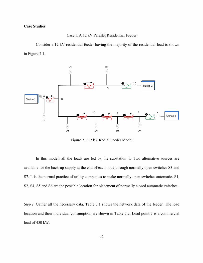
Case I: A 12 kV Parallel Residential Feeder

Consider a 12 kV residential feeder having the majority of the residential load is shown

in Figure 7.1.

Station 1

Station 2

Station 3

S3

XY

S2

XY

S7

XY

S4

XY

S5

XY

S6

XY

S1

XYA

B

C

D EF

CB

CB

CB

LP1

LP7LP6LP5LP4

LP2 LP3

Figure 7.1 12 kV Radial Feeder Model

In this model, all the loads are fed by the substation 1. Two alternative sources are

available for the back-up supply at the end of each node through normally open switches S3 and

S7. It is the normal practice of utility companies to make normally open switches automatic. S1,

S2, S4, S5 and S6 are the possible location for placement of normally closed automatic switches.

Step I: Gather all the necessary data. Table 7.1 shows the network data of the feeder. The load

location and their individual consumption are shown in Table 7.2. Load point 7 is a commercial

load of 450 kW.

43

Table 7.1 Network Data of the Residential Feeder

Failure Mode Failure Rate (λ) Total Length(miles)

A 0.15 4

B 0.15 4

C 0.15 4

D 0.15 4

E 0.15 4

F 0.15 4

Table 7.2 Load Data of the Residential Feeder

Load Point Average No. of Customers Average Load (KW)

1 133 900

2 100 850

3 133 900

4 100 890

5 133 900

6 133 700

7 10 450

Step II: Reliability Analysis

For reliability analysis, certain assumptions made in this thesis are mentioned below.

The system is radial.

All the faults are sustained.

The mean time to repair each of these feeder faults is assumed to be 2 hours.

The automatic switching time is 5 seconds.

The manual switching time is 1 hour.

The method of finding reliability parameters with different numbers of automatic

switches in a distribution system is a “combinatorial process”. Appendix A.7 lists the reliability

44

indices of the system for all possible placements of normally closed automatic switches. Table

7.3 lists the best value of reliability for the switch configuration with respective numbers of

normally closed automatic switches. ‘A’ stands for automatic switch and ‘M’ for manual switch.

Table 7.3 Reliability Indices for number of Automatic Switches in the Residential Feeder

No. of Automatic Switch Switch Configuration SAIFI SAIDI CMI

0 MMAMMMA 0.89 58.12 43128

1 MMAAMMA 0.44 36.32 26955

2 AMAAMMA 0.32 26.23 19467

3 AAAAMMA 0.25 19.37 14373

4 AAAAAMA 0.17 14.53 10782

5 AAAAAAA 0.14 14.53 10782

As automation increased, the reliability parameters (SAIFI, SAIDI and CMI)

significantly improved. This is due to a decrease in rate of power outage time. However,

automation increased reliability of the system to some point. After that point, there is no

significant benefit of automation as the reliability saturates. Figure 7.3 shows that the plot of

SAIFI and SAIDI improve as a result of an increase in automatic switches.

45

Figure 7.2 SAIFI and SAIDI Diagrams for 12 kV Residential Feeder

Step III: Economic Analysis

Even though reliability improved and saturated at some point, the number of automatic

switches after which saturation occurred might or might not be the optimal point. Proper

economic analysis must be done in order to figure out the optimal switch number and reliability

that can be achieved within a given budget. A proper benefit to cost analysis must be done for

this purpose.

For the economic analysis, the cost of the automatic switch is taken as $30,000

(IntelliRupter market value price) [19]. The interruption cost varies depending on the type of

customers. Table 7.4 lists the interruption cost for all type of customers for an hour according to

a survey report of The Midwest Independent Transmission System Operator [22].

0

0.2

0.4

0.6

0.8

1

0 2 4 6

SA

IFI

(Per

Yea

r)

Number of normally closed automatic switch

SAIFI

0

10

20

30

40

50

60

70

0 2 4 6

Inte

rru

pti

on

in

ho

urs

Number of normally closed automatic switch

SAIDI

46

Table 7.4 Interruption Cost per Kwh for Industrial, Commercial and Residential Load

Type of Customer Interruption Cost (per kWh)

Industrial $500-$600

Commercial $417

Residential $2

For different switch configurations, the interruption cost and total benefit is tabulated in

Table 7.5. Case ‘0’ is taken as a reference point. The total cost and benefits of partial and full

automation will be compared with respect to this reference point for economic analysis.

Table 7.5 Total Interruption Cost and Benefit for the Residential Load

Case Switch

Configuration

Switch Cost ($) Interruption Cost ($) Total Cost ($) Benefit ($) ΔB/ΔC

0 MMAMMMA 60,000.00 10,656.00 70,656.00 -

1 MMAAMMA 90,000.00 6,660.00 96,660.00 3,996.00 0.041

2 AMAAMMA 120,000.00 4,791.00 124,791.00 5,865.00 0.046

3 AAAAMMA 150,000.00 3,474.00 153,474.00 7,182.00 0.046

4 AAAAAMA 180,000.00 2,664.00 182,664.00 7,992.00 0.043

5 AAAAAAA 210,000.00 2,664.00 212,664.00 7,992.00 0.037

Figure 7.3 shows the plot of benefit to cost analysis of the 12 kV residential feeder. The

benefit considerably increased due to the increase in number of automatic switches. Then the

significant benefit of automation decreased. For this case, the optimal number of switches is 2.

47

Figure 7.3 Benefit to Cost Analysis of 12 kV Residential Feeder

Case II: A 12 kV Parallel Commercial Feeder

Step I: In this case, Figure 7.1 is remodeled with the majority of the commercial load. Table 7.6

shows the network data of the commercial feeder. The load location and their individual

consumption are shown in Table 7.7. Load point 7 is the industrial load of 2000 KW. Similarly,

load points 5 and 6 are the residential load.

Table 7.6 Network Data of the Commercial Feeder

Failure Mode Failure Rate (λ) Total Length(miles)

A 0.15 4

B 0.15 4

C 0.15 4

D 0.15 4

E 0.15 4

F 0.15 4

0

0.005

0.01

0.015

0.02

0.025

0.03

0.035

0.04

0.045

0.05

0 2 4 6

Ben

efit

to

co

st r

ati

o

Number of normally closed automatic switches

48

Table 7.7 Load Data of the Commercial Feeder

Load Point Avg No. of Customers Avg Load (KW)

LP1 40 1600

LP2 40 1700

LP3 20 850

LP4 40 1800

LP5 40 300

LP6 25 200

LP7 5 2000

Step II: Reliability Analysis

All the assumptions made for reliability analysis are the same as that for the residential

feeder. Appendix B.7 lists the reliability indices of the system for all possible placements for

normally closed automatic switches. Table 7.8 lists the configuration of normally closed switches

with the respective number of automatic switches for the best value of reliability. Figure 7.4

shows the plot of SAIFI and SAIDI improve as a result of an increase in automatic switches.

Table 7.8 Reliability Indices for number of Automatic Switches in the Commercial Feeder

No of automatic switch Switch configuration SAIFI SAIDI CMI

0 MMAMMMA 0.88 61.71 12960

1 MMAAMMA 0.44 38.57 8100

2 AMAAMMA 0.31 27.42 5760

3 AAAAMMA 0.24 20.57 4320

4 AAAAAMA 0.16 15.42 3240

5 AAAAAAA 0.14 15.42 3240

49

Figure 7.4 SAIFI and SAIDI Diagrams for 12 kV Commercial Feeder

Step III: Economic Analysis

For the economic analysis, all the assumptions made are the same as those for the

residential feeder. The interruption rates are also the same as in Table 7.4. The total benefit and

cost of different switch configuration for the commercial feeder is shown in Table 7.9

Table 7.9 Total Interruption Cost and Benefit for the Commercial Load

Case Switch

Configuration Switch Cost ($)

Interruption Cost

($) Total Cost ($) Benefit ($) ΔB/ΔC

0 MMAMMMA 60,000.00 2,978,100.00 3,038,100.00 -

1 MMAAMMA 90,000.00 1,861,312.50 1,951,312.50 1,116,787.50 0.57

2 AMAAMMA 120,000.00 1,176,390.00 1,296,390.00 1,801,710.00 1.38

3 AAAAMMA 150,000.00 744,795.00 894,795.00 2,233,305.00 2.49

4 AAAAAMA 180,000.00 744,525.00 924,525.00 2,233,575.00 2.41

5 AAAAAAA 210,000.00 744,525.00 954,525.00 2,233,575.00 2.33

Figure 7.5 shows the cost to benefit analysis of the 12 kV commercial feeder. The

benefits due to automation are significantly higher than as compared to the residential feeder. For

0

0.2

0.4

0.6

0.8

1

0 2 4 6

SA

IFI

(Per

Yea

r)

Number of normally closed automatic switch

SAIFI

0

10

20

30

40

50

60

70

0 2 4 6

Inte

rru

pti

on

in

ho

urs

Number of normally closed automatic switch

SAIDI

50

the commercial feeder, the optimal number of switches is 3 as the benefit to cost ratio starts to

decrease after this point.

Figure 7.5 Benefit to Cost Analysis of 12 kV Commercial Feeder

Case III: A 12 kV Parallel Industrial Feeder

Step I: Figure 7.1 is modified again with the majority of the industrial load. Table 7.10 shows the

network data of the industrial feeder. The load location and their individual consumption are

shown in Table 7.11. Load point 1 is the residential loads with consumption 144 KW. Similarly,

load points 6 and 7 are the commercial loads.

0

0.5

1

1.5

2

2.5

3

0 1 2 3 4 5 6

Ben

efit

to

co

st r

ati

o

Number of normally closed automatic switches

51

Table 7.10 Network Data of the Industrial Feeder

Failure Mode Failure Rate (λ) Total Length(miles)

A 0.15 4

B 0.15 4

C 0.15 4

D 0.15 4

E 0.15 4

F 0.15 4

Table 7.11 Load Data of the Industrial Feeder

Load Point Avg No. of Customers Avg Load (KW)

LP1 20 144

LP2 5 2500

LP3 5 4500

LP4 1 2000

LP5 5 2500

LP6 5 200

LP7 5 450

Step II: Reliability Analysis

Again, all the assumptions made for reliability analysis are the same as those for the

residential feeder. Appendix C.7 lists the reliability indices of the system for all possible

placements for normally closed automatic switches. Table 7.12 lists the configuration of

normally closed switches with the respective number of automatic switches for the best value of

reliability.

52

Table 7.12 Reliability Indices for number of Automatic Switches in the Industrial Feeder

No of Automatic Switch Switch Configuration SAIFI SAIDI CMI

0 MMAMMMA 0.782609 56.34783 2592

1 MAAMMMA 0.652174 44.41304 2043

2 MAAAMMA 0.26087 27.19565 1251

3 AAAAMMA 0.195652 17.02174 783

4 AAAAAMA 0.108696 14.08696 648

5 AAAAAAA 0.065217 14.08696 648

Figure 7.5 shows the plot of SAIFI and SAIDI improve as a result of an increase in

automatic switches.

Figure 7.6 SAIFI and SAIDI Diagrams for 12 kV Industrial Feeder

Step III: Economic Analysis

For the economic analysis, again all the assumptions made are the same as those for the

residential feeder. The interruption rates are mentioned in table 7.4. The total benefit and cost of

different switch configuration for industrial feeder is shown in table 7.13

0

0.1

0.2

0.3

0.4

0.5

0.6

0.7

0.8

0.9

0 2 4 6

SA

IFI

(Per

Yea

r)

Number of normally closed automatic switch

SAIFI

0

10

20

30

40

50

60

0 2 4 6

Inte

rru

pti

on

in

ho

urs

Number of normally closed automatic switch

SAIDI

53

Table 7.13 Total Interruption Cost and Benefit for the Industrial Load

Case Switch

Configuration

Switch Cost($) Interruption

Cost($)

Total Cost ($) Benefit ($) ΔB/ΔC

0 MMAMMMA 60,000.00 7,740,345.60 7,800,345.6 0 -

1 MAAMMMA 90,000.00 4,837,716.00 4,927,716.00 2,92,629.60 0.58

2 AAAAMMA 120,000.00 3,420,172.80 3,540,172.80 4,320,172.80 1.22

3 AAAAMMA 150,000.00 2,610,086.40 2,760,086.40 5,130,259.20 1.85

4 AAAAAMA 180,000.00 1,935,086.40 2,115,086.40 5,805,259.20 2.74

5 AAAAAAA 210,000.00 1,935,086.40 2,145,086.40 5,805,259.20 2.70

As shown in Table 7.13, the benefits due to automation are significantly higher as

compared to commercial as well as residential feeder. Figure 7.7 shows the benefit to cost ratio

for the industrial feeder. The optimal number of automatic switches for the industrial customer is

4.

Figure 7.7 Benefit to Cost Analysis of 12 kV Industrial Feeder

0

0.5

1

1.5

2

2.5

3

3.5

0 1 2 3 4 5 6

Ben

efit

to

co

st r

atio

Number of normally closed automatic switches

54

CHAPTER VIII

DISCUSSION AND CONCLUSION

This chapter discusses the findings of the case studies and the conclusion drawn by

comparing each model. Also, it briefly discusses the future implementation of the project.

Objectives of the Study

The main objective of the study is the reliability assessment of the automated distribution

system and to propose the optimum number and location of automatic switches that improve

reliability of the distribution system. A very simple analytical method has been implemented for

the system analysis. This research aims to help the manager and reliability engineers of the utility

company to understand the benefits and to perform economic analysis of the automation system.

Summary of the Findings

From the case studies conducted for residential, commercial and industrial feeders, the

following conclusions can be drawn.

a. The reliability of the system improves as the automation increases for all kinds of load

until a certain number of automatic switches are installed. After that, it saturates, i.e. no

more reliability improvement with further automation.

b. Benefit of automation is less for the residential load as compared to industrial and

commercial loads. This might be because the average consumption of the residential load

55

is very small compared to commercial and industrial loads even though they are large in

numbers. Figure 8.1 shows the comparison of benefit to cost ratio for residential,

industrial and commercial types of customers.

Figure 8.1 Comparison of Benefit to Cost Ratio of Industrial, Commercial and Residential Load

c. The number of automatic switches greatly depends upon the type of feeder. The number

of automatic switches is higher for industrial and commercial customers as compared to

the residential load. It may be due to the large interruption cost for the industrial and

commercial customers. Therefore, the utility companies are very concerned to provide

these kinds of customer a very reliable power supply at any cost. Generally big industries

have multiple feeders as they share the portion of reliability improvement with the utility

company.

d. Reliability of the distribution system greatly depends upon the placement of automatic

switches. The reliability indices for different numbers of automatic switches for all types

0

0.5

1

1.5

2

2.5

3

0 1 2 3 4 5 6

B/C

ra

tio

n

No. of normally closed switches

Residential

Industrial

Commercial

56

of feeders are shown in appendix A.7, B.7 and C.7. The reliability and benefits are

different for various switch locations even though the number of automatic switches is

the same.

Recommendations for Future Study

This thesis proposes a very simple analytical method for reliability assessment and

system economic analysis using an excel spreadsheet. However, this method can be very time

consuming if the number of load points are too high. In that case, simulation based methods can

be used to find optimal placement of automatic switches. Also, for the reliability evaluation, this

thesis accounts on the historic average data made available by utility companies. This model can

be further enhanced to real time data using Opal RT. Furthermore, the reliability and economic

analysis of the system with integration of DG (Distributed Generation) can be carried out.

57

REFERENCES

[1] R. Billinton and S. Jonnavithula, "Optimal switching device placement in radial distribution

systems," IEEE Transactions on Power Delivery, vol. 11 , no. 3, pp. 1646-1651, Jul 1996.

[2] H. Najafi, "Optimal Allocation and Number of Automatic Switches in Distribution

Networks," pp. 1-6.

[3] K. Alekhya, P. Murthy and C. Bhargava, "Assessment of Reliability for Distribution

Feeders on the Basis of Cost Analysis," Bonfiring International Journal of Power Systems

and Integrated Circuits, Vol.1, pp. 15-19, 2011.

[4] C.-S. Chen, C.-H. Lin and H.-j. Chuang, "Optimal Placement of Line Switches for

Distribution Automation Systems Using Immune Algorithm," IEEE Transactions on Power

Systems, vol. 21, no. 3, pp. 1209-1217, 2006.

[5] A. Kazemi and F. T. Asr, "Determining Optimum Location of Automated Switches in

Distribution Network," 2008.

[6] G. Sardou, M. Banejad, R. Hooshmand and A. Dastfan, "Modified Shuffled frog leaping

algorithm for optimal switch placement in distribution automation sytem using a mulit-

objective fuzzy approach," IET Generation, Transmission and Distribution, pp. 493-502,

2011.

[7] R. E. Brown, "Reliability Metrices and Indices," in Electric Power Distribution Reliability,

New York, CRC Press, 2009, pp. 41-102.

[8] M. M. J. S. Michael J. Sullivan, "Estimated Value of Service Reliability for Electric Utility

Customers in the United States," June 2009. [Online]. Available:

http://certs.lbl.gov/pdf/lbnl-2132e.pdf.

[9] R. Billinton and R. N. Allan, Reliability Evaluation of Power Systems, Plenum press, 1996.

[10] P. Bhusal, "Distribution Reliability Analysis," Wichita State University, Kansas, 2007.

[11] R. E. Brown, "Interruption causes," in Electric Power Distrubution Reliability, New York,

CRC Press, 2009, pp. 107-157.

58

[12] "Guy Wire," Wikipedia, October 2007. [Online]. Available: en.wikipedia.org/wiki/Guy-

wire.

[13] "SEL 321 Relay," schweitzer Engineering Laboratories, [Online]. Available:

https://www.selinc.com/SEL-321/.

[14] "circuit breaker," TEXAS ENGINEERING, [Online]. Available:

http://smartgridcenter.tamu.edu/ratc/.

[15] J. J. Burke, "Reclosers," in Power Distribution Engineering, New York, Marcel Dekker,

1994, pp. 124-125.

[16] "Three Phase Vacuum Reclosers and Control Modules," northeastpowerdelivery, [Online].

Available: http://www.northeastpowerdelivery.com/content/northeast-power-delivery-

vacuum-reclosers-control-modules/.

[17] "Switchgear," [Online]. Available: http://en.wikipedia.org/wiki/Switchgear.

[18] A. Helseth and A. T. Holen, "Impact of Energy End use and customer interruption cost on

optimal allocation of switchgear in constrained distribution networks," IEEE transactions

on power delivery, pp. 1-7, 2007.

[19] "S&C IntelliRupter PulseCloser," S&C Electric Company, 14 May 2012. [Online].

Available: http://www.sandc.com/support/publications/intellirupter-pulsecloser-pubs.asp.

[20] Z. Bozic, "Customer interruption cost calculation for reliability economics: practical

considerations," in International Conference on Power System Technology, Perth, WA ,

2000.

[21] R. E. Brown, "System Analysis," in Electric Power Distribution Reliablity, New York,

CRC Press, 2009, pp. 265-357.

[22] P. Centolella, "Estimates of the Value of Uninterrupted Service for The Mid-West

Independent System Operator," 2005. [Online]. Available:

http://www.hks.harvard.edu/hepg/Papers/2010/VOLL%20Final%20Report%20to%20MISO

%20042806.pdf.

59

APPENDIX A

RELIABILITY ASSESSMENT AND ECONOMIC ANALYSIS OF THE RESIDENTIAL

FEEDER

60

Table A.1 Switch Placement Module for the Residential Feeder

Switch position Type Switching time MTTR

1 1 0.001388889 2

2 1 0.001388889 2

3 1 0.001388889 2

4 1 0.001388889 2

5 1 0.001388889 2

6 1 0.001388889 2

7 1 0.001388889 2

No. of Automatic switch 7

**1=Automatic, 0=Manual, Automatic Switching time =5 sec= 0.001388889 hr

Table A.2 Reliability Indices for Switch Module shown in Table A.1

SAIFI (INT/CUST) 0.144204852

SAIDI (min/CUST INT) 14.5309973

CAIDI(min/Int) 100.7663551

ASAI 0.99834121

CMI 10782

Interruption cost $ 2,664.00

61

Table A.3 Power availability Rate for all Load Points Depending upon Switch Module shown in A.1 using FMEA Method for the

Residential Feeder

Fa

ult

Load point (LP1) Load point (LP2) Load point (LP3) Load point (LP4) Load point (LP5) Load point (LP6) Load point (LP7)

λ

(f/y

r)

r (hr) U=λ.r (hr/yr)

λ

(f/yr

)

r (hr) U=λ.r (hr/yr)

λ

(f/y

r)

r (hr) U=λ.r (hr/yr)

λ

(f/yr

)

r (hr) U=λ.r (hr/yr)

λ

(f/y

r)

r (hr) U=λ.r (hr/yr)

λ (f/yr)

r (hr)

U=λ.r (hr/yr)

λ (f/yr)

r (hr)

U=λ.r (hr/yr)

A 0.1

5 2 0.3 0.15

0.00138888

9 0

0.1

5

0.0013

88889 0 0.15

0.0013888

9 0

0.1

5

0.00

1389 0 0.15

0.0013

89 0 0.15

0.0013

89 0

B 0.1

5

0.0013

88889 0 0.15 2 0.3

0.1

5

0.0013

88889 0 0.15 2 0.3

0.1

5

0.00

1389 0 0.15

0.0013

89

0 0.15

0.0013

89

0

C 0.1

5

0.0013

88889 0 0.15

0.001

388889

0 0.1

5 2 0.3 0.15

0.001

38889

0 0.1

5

0.00

1389 0 0.15

0.0

01389

0 0.15

0.0

01389

0

D 0.1

5

0.0013

88889 0 0.15

0.001

388889

0 0.1

5

0.0013

88889 0 0.15

0.001

38889

0 0.1

5 2 0.3 0.15

0.0

01389

0 0.15

0.0

01389

0

E 0.1

5

0.001388889

0 0.15

0.001

38888

9 0

0.1

5

0.001388889

0 0.15

0.001

3888

9 0

0.1

5

0.001389

0 0.15 2 0.3 0.15

0.0

013

89 0

F 0.1

5

0.001388889

0 0.15

0.001

38888

9 0

0.1

5

0.001388889

0 0.15

0.001

3888

9 0

0.1

5

0.001389

0 0.15

0.0

013

89 0 0.15 2 0.3

∑

λ 0.9

0.3 0.9

0.3 0.9

0.3 0.9

0.3 0.9

0.3 0.9

0.3 0.9

0.3

Table A.4 Number of Customer Interruption for different Failure Modes Depending on Switch Module shown in A.1

Compone

nts Failure rate

(λ/yr) Total No of customer

interrupted Customer

Interruption (CI) Avg no of momentary

interruption Cust Momentary

Interruption

A 0.15 133 19 609 91

B 0.15 200 30 542 81

C 0.15 133 19 609 91

D 0.15 133 19 609 91

E 0.15 133 19 609 91

F 0.15 10 1 732 109

107 554

62

Table A.5 Customer Minute Interruption for all Load Points in the Residential Feeder

Load Point Avg No. of Customers (N) U(λ.r) CMI (N*U*60 min)

LP1 133 0.3 2394

LP2 100 0.3 1800

LP3 133 0.3 2394

LP4 100 0.3 1800

LP5 133 0.3 2394

LP6 133 0.3 2394

LP7 10 0.3 180

10782

Table A.6 Customer Interruption Cost for Different Loads Depending on their Rates

Load Point Interruption cost rate ($/kWhr) Avg. Load (kW) Interruption rate (hr/yr) Interruption cost ($)

LP1 2 900 0.3 $ 540.00

LP2 2 850 0.3 $ 510.00

LP3 2 900 0.3 $ 540.00

LP4 2 890 0.3 $ 534.00

LP5 2 900 0.3 $ 540.00

LP6 2 700 0.3 $ 420.00

LP7 417 450 0.3 $ 56,295.00

Total Interruption cost $ 2,664.00

63

Table A.7 Detail Reliability and Economic Analysis Sorted based on B/C Ratio for Different Number and Switch Locations for the

Residential Feeder

No. of NC automatic SwitchesS1 S2 S3 S4 S5 S6 S7 SAIFI SAIDI CMI Switch Cost INTERRUPTION COST Total Cost Benefit ΔB/ΔC CMI savings $/CMI Savings

0 0 0 1 0 0 0 1 0.897574 58.12399 43128 60,000.00$ 10,656.00$ 70,656.00$ -$

1 0 0 1 0 0 1 1 0.735849 50.85849 37737 90,000.00$ 9,324.00$ 99,324.00$ 1,332.00$ 0.013410656 5391 18.42$

1 0 0 1 0 1 0 1 0.536388 43.59299 32346 90,000.00$ 7,992.00$ 97,992.00$ 2,664.00$ 0.027185893 10782 9.09$

1 0 1 1 0 0 0 1 0.638814 42.79245 31752 90,000.00$ 7,974.00$ 97,974.00$ 2,682.00$ 0.02737461 11376 8.61$

1 1 0 1 0 0 0 1 0.638814 42.79245 31752 90,000.00$ 7,974.00$ 97,974.00$ 2,682.00$ 0.02737461 11376 8.61$

1 0 0 1 1 0 0 1 0.444744 36.32749 26955 90,000.00$ 6,660.00$ 96,660.00$ 3,996.00$ 0.041340782 16173 5.98$

2 0 0 1 0 1 1 1 0.506739 43.59299 32346 120,000.00$ 7,992.00$ 127,992.00$ 2,664.00$ 0.020813801 10782 11.87$

2 0 1 1 0 0 1 1 0.506739 37.14016 27558 120,000.00$ 6,912.00$ 126,912.00$ 3,744.00$ 0.029500756 15570 8.15$

2 1 0 1 0 0 1 1 0.506739 37.14016 27558 120,000.00$ 6,912.00$ 126,912.00$ 3,744.00$ 0.029500756 15570 8.15$

2 0 0 1 1 0 1 1 0.385445 34.71429 25758 120,000.00$ 6,390.00$ 126,390.00$ 4,266.00$ 0.03375267 17370 7.28$

2 0 0 1 1 1 0 1 0.361186 31.48787 23364 120,000.00$ 5,850.00$ 125,850.00$ 4,806.00$ 0.038188319 19764 6.37$

2 0 1 1 0 1 0 1 0.361186 31.48787 23364 120,000.00$ 5,850.00$ 125,850.00$ 4,806.00$ 0.038188319 19764 6.37$

2 1 0 1 0 1 0 1 0.361186 31.48787 23364 120,000.00$ 5,850.00$ 125,850.00$ 4,806.00$ 0.038188319 19764 6.37$

2 1 1 1 0 0 0 1 0.433962 29.47439 21870 120,000.00$ 5,577.00$ 125,577.00$ 5,079.00$ 0.040445304 21258 5.91$

2 0 1 1 1 0 0 1 0.32345 27.44879 20367 120,000.00$ 5,058.00$ 125,058.00$ 5,598.00$ 0.04476323 22761 5.49$

2 1 0 1 1 0 0 1 0.32345 26.23585 19467 120,000.00$ 4,791.00$ 124,791.00$ 5,865.00$ 0.046998582 23661 5.27$

3 0 0 1 1 1 1 1 0.331536 31.48787 23364 150,000.00$ 5,850.00$ 155,850.00$ 4,806.00$ 0.030837344 19764 7.89$

3 0 1 1 0 1 1 1 0.331536 31.48787 23364 150,000.00$ 5,850.00$ 155,850.00$ 4,806.00$ 0.030837344 19764 7.89$

3 1 0 1 0 1 1 1 0.331536 31.48787 23364 150,000.00$ 5,850.00$ 155,850.00$ 4,806.00$ 0.030837344 19764 7.89$

3 0 1 1 1 0 1 1 0.264151 25.83558 19170 150,000.00$ 4,788.00$ 154,788.00$ 5,868.00$ 0.037909915 23958 6.46$

3 1 1 1 0 0 1 1 0.331536 25.43531 18873 150,000.00$ 4,785.00$ 154,785.00$ 5,871.00$ 0.037930032 24255 6.38$

3 1 0 1 1 0 1 1 0.264151 24.62264 18270 150,000.00$ 4,521.00$ 154,521.00$ 6,135.00$ 0.039703341 24858 6.22$

3 0 1 1 1 1 0 1 0.239892 22.60916 16776 150,000.00$ 4,248.00$ 154,248.00$ 6,408.00$ 0.041543488 26352 5.85$

3 1 1 1 0 1 0 1 0.239892 21.39623 15876 150,000.00$ 3,993.00$ 153,993.00$ 6,663.00$ 0.043268201 27252 5.65$

3 1 0 1 1 1 0 1 0.239892 21.39623 15876 150,000.00$ 3,981.00$ 153,981.00$ 6,675.00$ 0.043349504 27252 5.65$

3 1 1 1 1 0 0 1 0.257412 19.37062 14373 150,000.00$ 3,474.00$ 153,474.00$ 7,182.00$ 0.0467962 28755 5.34$

4 0 1 1 1 1 1 1 0.210243 22.60916 16776 180,000.00$ 4,248.00$ 184,248.00$ 6,408.00$ 0.034779211 26352 6.99$

4 1 1 1 0 1 1 1 0.210243 21.39623 15876 180,000.00$ 3,993.00$ 183,993.00$ 6,663.00$ 0.036213334 27252 6.75$

4 1 0 1 1 1 1 1 0.210243 21.39623 15876 180,000.00$ 3,981.00$ 183,981.00$ 6,675.00$ 0.03628092 27252 6.75$

4 1 1 1 1 0 1 1 0.198113 17.75741 13176 180,000.00$ 3,204.00$ 183,204.00$ 7,452.00$ 0.040675968 29952 6.12$

4 1 1 1 1 1 0 1 0.173854 14.531 10782 180,000.00$ 2,664.00$ 182,664.00$ 7,992.00$ 0.043752464 32346 5.65$

5 1 1 1 1 1 1 1 0.144205 14.531 10782 210,000.00$ 2,664.00$ 212,664.00$ 7,992.00$ 0.037580409 32346 6.57$

64

APPENDIX B

RELIABILITY ASSESSMENT AND ECONOMIC ANALYSIS OF THE COMMERCIAL

FEEDER

65

Table B.1 Switch Placement Module for the Commercial Feeder

Switch position Type Switching time MTTR

1 1 0.001388889 2

2 1 0.001388889 2

3 1 0.001388889 2

4 1 0.001388889 2

5 1 0.001388889 2

6 1 0.001388889 2

7 1 0.001388889 2

No. of Automatic switch 7

**1=Automatic, 0=Manual, Automatic Switching time =5 sec= 0.001388889 hr

Table B.2 Reliability Indices for Switch Module Shown in Table B.1

SAIFI (INT/CUST) 0.142857143

SAIDI (min/CUST INT) 15.42857143

CAIDI(min/Int) 108

ASAI 0.998238748

CMI 3240

Interruption cost $ 744,525.00

66

Table B.3 Power Availability Rate for all Load Points Depending upon Switch Module shown in B.1 using FMEA Method for the

Commercial Feeder

Fa

ult

Load point (LP1) Load point (LP2) Load point (LP3) Load point (LP4) Load point (LP5) Load point (LP6) Load point (LP7)

λ

(f/y

r)

r (hr) U=λ.r

(hr/yr)

λ

(f/y

r)

r (hr) U=λ.r

(hr/yr)

λ

(f/y

r)

r (hr) U=λ.r

(hr/yr)

λ

(f/y

r)

r (hr) U=λ.r

(hr/yr)

λ

(f/y

r)

r

(hr)

U=λ.r

(hr/yr)

λ

(f/y

r)

r

(hr)

U=λ.r

(hr/yr)

λ

(f/y

r)

r

(hr)

U=λ.r

(hr/yr)

A 0.1

5 2 0.3

0.1

5

0.0013

88889 0

0.1

5

0.0013

88889 0

0.1

5

0.001

38889 0

0.1

5

0.00

1389 0

0.1

5

0.00

1389 0

0.1

5

0.00

1389 0

B 0.1

5

0.0013

88889 0

0.1

5 2 0.3

0.1

5

0.0013

88889 0

0.1

5 2 0.3

0.1

5

0.00

1389 0

0.1

5

0.00

1389 0

0.1

5

0.00

1389 0

C 0.1

5

0.0013

88889 0

0.1

5

0.0013

88889 0

0.1

5 2 0.3

0.1

5

0.001

38889 0

0.1

5

0.00

1389 0

0.1

5

0.00

1389 0

0.1

5

0.00

1389 0

D 0.1

5

0.0013

88889 0

0.1

5

0.0013

88889 0

0.1

5

0.0013

88889 0

0.1

5

0.001

38889 0

0.1

5 2 0.3

0.1

5

0.00

1389 0

0.1

5

0.00

1389 0

E 0.1

5

0.0013

88889 0

0.1

5

0.0013

88889 0

0.1

5

0.0013

88889 0

0.1

5

0.001

38889 0

0.1

5

0.00

1389 0

0.1

5 2 0.3

0.1

5

0.00

1389 0

F 0.1

5

0.0013

88889 0

0.1

5

0.0013

88889 0

0.1

5

0.0013

88889 0

0.1

5

0.001

38889 0

0.1

5

0.00

1389 0

0.1

5

0.00

1389 0

0.1

5 2 0.3

∑λ 0.9

0.3 0.9

0.3 0.9

0.3 0.9

0.3 0.9

0.3 0.9

0.3 0.9

0.3

Table B.4 Number of Customer Interruption for different failure modes depending on switch module shown in B.1

Number of customers A B C D E F

40 2 0.001388889 0.001388889 0.001388889 0.001388889 0.001388889

40 0.001388889 2 0.001388889 0.001388889 0.001388889 0.001388889

20 0.001388889 0.001388889 2 0.001388889 0.001388889 0.001388889

40 0.001388889 2 0.001388889 0.001388889 0.001388889 0.001388889

40 0.001388889 0.001388889 0.001388889 2 0.001388889 0.001388889

25 0.001388889 0.001388889 0.001388889 0.001388889 2 0.001388889

5 0.001388889 0.001388889 0.001388889 0.001388889 0.001388889 2

Average load affected 40 80 20 40 25 5

67

Table B.5 Customer Minute Interruption for all Load Points in the Commercial Feeder

Faul

ts Failure rate

(λ/yr) Avg. No of customer

interrupted Customer Interruption

(CI) Avg no of momentary

interruption Cust Momentary

Interruption

A 0.15 40 6 170 25

B 0.15 80 12 130 19

C 0.15 20 3 190 28

D 0.15 40 6 170 25

E 0.15 25 3 185 27

F 0.15 5 0 205 30

30

154

Table B.6 Customer Interruption Cost for Different Loads Depending their Rates

Load Point Interruption cost rate ($/kWhr) Avg. Load (kW) Interruption rate (hr/yr) Interruption cost ($)

LP1 417 1600 0.3 $ 200,160.00

LP2 417 1700 0.3 $ 212,670.00

LP3 417 850 0.3 $ 106,335.00

LP4 417 1800 0.3 $ 225,180.00

LP5 2 300 0.3 $ 180.00

LP6 2 200 0.3 $ 120.00

LP7 45 2000 0.3 $ 27,000.00

Total Interruption cost $ 744,525.00

68

Table B.7 Detail Reliability and Economic Analysis Sorted based on B/C Ratio For Different Number and Switch Locations for the

Commercial Feeder

No. of NC Aut switch S1 S2 S3 S4 S5 S6 S7 SAIFI SAIDI CMI Switch Cost INTERRUPTION COST Total Cost Benefit ΔB/ΔC CMI savings $/CMI Savings

0 0 0 1 0 0 0 1 0.885714 61.71429 12960 60,000.00$ 2,978,100.00$ 3,038,100.00$ -$

1 0 0 1 0 0 1 1 0.714286 54 11340 90,000.00$ 2,605,837.50$ 2,695,837.50$ 372,262.50$ 0.138087885 1620 1,664.10$

1 0 1 1 0 0 0 1 0.680952 49.71429 10440 90,000.00$ 2,340,000.00$ 2,430,000.00$ 638,100.00$ 0.262592593 2520 964.29$

1 0 0 1 0 1 0 1 0.552381 46.28571 9720 90,000.00$ 2,233,575.00$ 2,323,575.00$ 744,525.00$ 0.320422194 3240 717.15$

1 1 0 1 0 0 0 1 0.62381 45.42857 9540 90,000.00$ 2,105,437.50$ 2,195,437.50$ 872,662.50$ 0.397489111 3420 641.94$

1 0 0 1 1 0 0 1 0.442857 38.57143 8100 90,000.00$ 1,861,312.50$ 1,951,312.50$ 1,116,787.50$ 0.572326319 4860 401.50$

2 0 0 1 0 1 1 1 0.528571 46.28571 9720 120,000.00$ 2,233,575.00$ 2,353,575.00$ 744,525.00$ 0.316337911 3240 726.41$

2 0 1 1 0 0 1 1 0.528571 42.85714 9000 120,000.00$ 2,020,905.00$ 2,140,905.00$ 957,195.00$ 0.447098307 3960 540.63$

2 0 0 1 1 0 1 1 0.385714 36.85714 7740 120,000.00$ 1,861,222.50$ 1,981,222.50$ 1,116,877.50$ 0.563731484 5220 379.54$

2 0 0 1 1 1 0 1 0.366667 33.42857 7020 120,000.00$ 1,861,042.50$ 1,981,042.50$ 1,117,057.50$ 0.563873567 5940 333.51$

2 1 0 1 0 0 1 1 0.485714 39.42857 8280 120,000.00$ 1,833,255.00$ 1,953,255.00$ 1,144,845.00$ 0.586121628 4680 417.36$

2 0 1 1 0 1 0 1 0.395238 36 7560 120,000.00$ 1,701,810.00$ 1,821,810.00$ 1,276,290.00$ 0.700561529 5400 337.37$

2 1 0 1 0 1 0 1 0.366667 33.42857 7020 120,000.00$ 1,561,072.50$ 1,681,072.50$ 1,417,027.50$ 0.842930629 5940 283.01$

2 1 1 1 0 0 0 1 0.461905 34.28571 7200 120,000.00$ 1,514,250.00$ 1,634,250.00$ 1,463,850.00$ 0.895731987 5760 283.72$

2 0 1 1 1 0 0 1 0.328571 30.85714 6480 120,000.00$ 1,382,805.00$ 1,502,805.00$ 1,595,295.00$ 1.061544911 6480 231.91$

2 1 0 1 1 0 0 1 0.314286 27.42857 5760 120,000.00$ 1,176,390.00$ 1,296,390.00$ 1,801,710.00$ 1.389790109 7200 180.05$

3 0 0 1 1 1 1 1 0.342857 33.42857 7020 150,000.00$ 1,861,042.50$ 2,011,042.50$ 1,117,057.50$ 0.555461906 5940 338.56$

3 0 1 1 0 1 1 1 0.371429 36 7560 150,000.00$ 1,701,810.00$ 1,851,810.00$ 1,276,290.00$ 0.689212176 5400 342.93$

3 1 0 1 0 1 1 1 0.342857 33.42857 7020 150,000.00$ 1,561,072.50$ 1,711,072.50$ 1,417,027.50$ 0.828151642 5940 288.06$

3 0 1 1 1 0 1 1 0.271429 29.14286 6120 150,000.00$ 1,382,715.00$ 1,532,715.00$ 1,595,385.00$ 1.040888228 6840 224.08$

3 0 1 1 1 1 0 1 0.252381 25.71429 5400 150,000.00$ 1,382,535.00$ 1,532,535.00$ 1,595,565.00$ 1.041127935 7560 202.72$

3 1 1 1 0 0 1 1 0.342857 29.14286 6120 150,000.00$ 1,295,235.00$ 1,445,235.00$ 1,682,865.00$ 1.164423087 6840 211.29$

3 1 0 1 1 0 1 1 0.257143 25.71429 5400 150,000.00$ 1,176,300.00$ 1,326,300.00$ 1,801,800.00$ 1.358516173 7560 175.44$

3 1 0 1 1 1 0 1 0.238095 22.28571 4680 150,000.00$ 1,176,120.00$ 1,326,120.00$ 1,801,980.00$ 1.358836304 8280 160.16$

3 1 1 1 0 1 0 1 0.252381 24 5040 150,000.00$ 1,076,220.00$ 1,226,220.00$ 1,901,880.00$ 1.551010422 7920 154.83$

3 1 1 1 1 0 0 1 0.242857 20.57143 4320 150,000.00$ 744,795.00$ 894,795.00$ 2,233,305.00$ 2.495884532 8640 103.56$

4 0 1 1 1 1 1 1 0.228571 25.71429 5400 180,000.00$ 1,382,535.00$ 1,562,535.00$ 1,595,565.00$ 1.021138726 7560 206.68$

4 1 0 1 1 1 1 1 0.214286 22.28571 4680 180,000.00$ 1,176,120.00$ 1,356,120.00$ 1,801,980.00$ 1.328776214 8280 163.78$

4 1 1 1 0 1 1 1 0.228571 24 5040 180,000.00$ 1,076,220.00$ 1,256,220.00$ 1,901,880.00$ 1.513970483 7920 158.61$

4 1 1 1 1 0 1 1 0.185714 18.85714 3960 180,000.00$ 744,705.00$ 924,705.00$ 2,233,395.00$ 2.41525135 9000 102.75$

4 1 1 1 1 1 0 1 0.166667 15.42857 3240 180,000.00$ 744,525.00$ 924,525.00$ 2,233,575.00$ 2.415916281 9720 95.12$

5 1 1 1 1 1 1 1 0.142857 15.42857 3240 210,000.00$ 744,525.00$ 954,525.00$ 2,233,575.00$ 2.339985857 9720 98.20$

69

APPENDIX C

RELIABILITY ASSESSMENT AND ECONOMIC ANALYSIS OF THE INDUSTRIAL

FEEDER

70

Table C.1 Switch Placement Module for the Industrial Load

Switch position Type Switching time MTTR

1 1 0.001388889 2

2 1 0.001388889 2

3 1 0.001388889 2

4 1 0.001388889 2

5 1 0.001388889 2

6 1 0.001388889 2

7 1 0.001388889 2

No. of Automatic switch 7

**1=Automatic, 0=Manual, Automatic Switching time =5 sec= 0.001388889 hr

Table C.2 Reliability Indices for Switch Module shown in Table C.1

SAIFI (INT/CUST) 0.065217391

SAIDI (min/CUST INT) 14.08695652

CAIDI(min/Int) 216

ASAI 0.9983919

CMI 648

Interruption cost $ 1,935,086.40

71

Table C.3 Power Availability Rate for all Load Points Depending upon Switch Module shown in C.1 using FMEA Method for the

Industrial Feeder

Failur

e

Comp

onent

Load point (LP1) Load point (LP2) Load point (LP3) Load point (LP4) Load point (LP5) Load point (LP6) Load point (LP7)

λ

(f/yr) r (hr)

U=λ.r

(hr/yr

)

λ

(f/yr

)

r (hr)

U=λ

.r

(hr/

yr)

λ

(f/yr

)

r (hr) U=λ.r

(hr/yr)

λ

(f/y

r)

r (hr) U=λ.r

(hr/yr)

λ

(f/yr

)

r

(hr)

U=λ.r

(hr/y

r)

λ

(f/yr

)

r

(hr)

U=λ

.r

(hr/

yr)

λ

(f/yr

)

r

(hr)

U=λ.r

(hr/yr)

A 0.15 2 0.3 0.15 5sec 0 0.15 5sec 0 0.15 5sec 0 0.15 5sec 0 0.15 5sec 0 0.15 5sec 0

B 0.15 5sec 0 0.15 2 0.3 0.15 5sec 0 0.15 2 0.3 0.15 0.00

1389 0 0.15

0.00

1389 0 0.15 5sec 0

C 0.15 5sec 0 0.15 5sec 0 0.15 2 0.3 0.15 5sec 0 0.15 5sec 0 0.15 5sec 0 0.15 5sec 0

D 0.15 5sec 0 0.15 5sec 0 0.15 5sec 0 0.15 5sec 0 0.15 2 0.3 0.15 5sec 0 0.15 5sec 0

E 0.15 5sec 0 0.15 5sec 0 0.15 5sec 0 0.15 5sec 0 0.15 5sec 0 0.15 2 0.3 0.15 5sec 0

F 0.15 5sec 0 0.15 5sec 0 0.15 5sec 0 0.15 5sec 0 0.15 0.00

1389 0 0.15 5sec 0 0.15 2 0.3

∑λ 0.9

0.3 0.9

0.3 0.9

0.3 0.9

0.3 0.9

0.3 0.9

0.3 0.9

0.3

Table C.4 Number of Customer Interruption for Different Failure Modes Depending on Switch Module shown in C.1

Compone

nts Failure rate

(λ/yr) Avg. No of customer

interrupted Customer

Interruption (CI) Avg no of momentary

interruption Cust Momentary

Interruption

A 0.15 20 3 26 3

B 0.15 6 0 40 6

C 0.15 5 0 41 6

D 0.15 5 0 41 6

E 0.15 5 0 41 6

F 0.15 5 0 41 6

3

33

72

Table C.5 Customer Minute Interruption for all Load Points in the Industrial Feeder

Load Point Avg No. of Customers U(λ.r) CMI (Customer minute Interruption)

LP1 20 0.3 360

LP2 5 0.3 90

LP3 5 0.3 90

LP4 1 0.3 18

LP5 5 0.3 90

LP6 5 0.3 90

LP7 5 0.3 90

648

Table C.6 Customer Interruption Cost for Different Loads Depending on their Rates

Load Point Interruption cost rate ($/kWhr) Avg. Load (kW) Interruption rate (hr/yr) Interruption cost ($)

LP1 2 144 0.3 $ 86.40

LP2 600 2500 0.3 $ 450,000.00

LP3 500 4500 0.3 $ 675,000.00

LP4 600 2000 0.3 $ 360,000.00

LP5 600 2500 0.3 $ 450,000.00

LP6 417 200 0.3 $ 25,020.00

LP7 417 450 0.3 $ 56,295.00

Total Interruption cost $ 1,935,086.40

73

Table C.7 Detail Reliability and Economic Analysis Sorted based on B/C Ratio For Different Number and Switch Locations for the

Industrial Feeder

No. of NC Automated Switches S1 S2 S3 S4 S5 S6 S7 SAIFI SAIDI CMI Switch Cost INTERRUPTION COST Total Cost Benefit ΔB/ΔC CMI savings $/CMI Savings

0 0 0 1 0 0 0 1 0.782609 56.34783 2592 60,000.00$ 7,740,345.60$ 7,800,345.60$ -$

1 0 0 1 0 0 1 1 0.652174 49.30435 2268 90,000.00$ 6,772,802.40$ 6,862,802.40$ 967,543.20$ 0.140983689 324 21,181.49$

1 1 0 1 0 0 0 1 0.391304 29.73913 1368 90,000.00$ 6,772,586.40$ 6,862,586.40$ 967,759.20$ 0.141019602 1224 5,606.69$

1 0 0 1 0 1 0 1 0.478261 42.26087 1944 90,000.00$ 5,805,259.20$ 5,895,259.20$ 1,935,086.40$ 0.328244499 648 9,097.62$

1 0 1 1 0 0 0 1 0.652174 44.41304 2043 90,000.00$ 5,085,302.40$ 5,175,302.40$ 2,655,043.20$ 0.513021848 549 9,426.78$

1 0 0 1 1 0 0 1 0.391304 35.21739 1620 90,000.00$ 4,837,716.00$ 4,927,716.00$ 2,902,629.60$ 0.589041576 972 5,069.67$

2 0 0 1 0 1 1 1 0.434783 42.26087 1944 120,000.00$ 5,805,259.20$ 5,925,259.20$ 1,935,086.40$ 0.326582574 648 9,143.92$

2 1 0 1 0 0 1 1 0.326087 26.6087 1224 120,000.00$ 5,805,086.40$ 5,925,086.40$ 1,935,259.20$ 0.326621262 1368 4,331.20$

2 1 0 1 0 1 0 1 0.23913 23.47826 1080 120,000.00$ 4,837,586.40$ 4,957,586.40$ 2,902,759.20$ 0.585518631 1512 3,278.83$

2 0 0 1 1 0 1 1 0.304348 34.23913 1575 120,000.00$ 4,612,716.00$ 4,732,716.00$ 3,127,629.60$ 0.660853007 1017 4,653.60$

2 0 1 1 0 0 1 1 0.434783 38.34783 1764 120,000.00$ 4,455,259.20$ 4,575,259.20$ 3,285,086.40$ 0.718010993 828 5,525.68$

2 1 1 1 0 0 0 1 0.326087 21.71739 999 120,000.00$ 4,230,086.40$ 4,350,086.40$ 3,510,259.20$ 0.80694011 1593 2,730.75$

2 0 0 1 1 1 0 1 0.304348 32.28261 1485 120,000.00$ 4,162,716.00$ 4,282,716.00$ 3,577,629.60$ 0.835364661 1107 3,868.76$

2 1 0 1 1 0 0 1 0.23913 21.13043 972 120,000.00$ 3,915,086.40$ 4,035,086.40$ 3,825,259.20$ 0.947999329 1620 2,490.79$

2 0 1 1 0 1 0 1 0.304348 32.28261 1485 120,000.00$ 3,825,216.00$ 3,945,216.00$ 3,915,129.60$ 0.992373954 1107 3,563.88$

2 0 1 1 1 0 0 1 0.26087 27.19565 1251 120,000.00$ 3,420,172.80$ 3,540,172.80$ 4,320,172.80$ 1.220328228 1341 2,639.95$

3 1 0 1 0 1 1 1 0.195652 23.47826 1080 150,000.00$ 4,837,586.40$ 4,987,586.40$ 2,902,759.20$ 0.581996775 1512 3,298.67$

3 0 0 1 1 1 1 1 0.26087 32.28261 1485 150,000.00$ 4,162,716.00$ 4,312,716.00$ 3,577,629.60$ 0.82955372 1107 3,895.86$

3 0 1 1 0 1 1 1 0.26087 32.28261 1485 150,000.00$ 3,825,216.00$ 3,975,216.00$ 3,915,129.60$ 0.984884746 1107 3,590.98$

3 1 0 1 1 0 1 1 0.152174 20.15217 927 150,000.00$ 3,690,086.40$ 3,840,086.40$ 4,050,259.20$ 1.054731269 1665 2,306.36$

3 1 1 1 0 0 1 1 0.195652 19.56522 900 150,000.00$ 3,600,086.40$ 3,750,086.40$ 4,140,259.20$ 1.104043683 1692 2,216.36$

3 1 0 1 1 1 0 1 0.152174 18.19565 837 150,000.00$ 3,240,086.40$ 3,390,086.40$ 4,500,259.20$ 1.327476255 1755 1,931.67$

3 0 1 1 1 0 1 1 0.173913 26.21739 1206 150,000.00$ 3,195,172.80$ 3,345,172.80$ 4,545,172.80$ 1.358725863 1386 2,413.54$

3 1 1 1 0 1 0 1 0.152174 17.41304 801 150,000.00$ 2,970,086.40$ 3,120,086.40$ 4,770,259.20$ 1.528886892 1791 1,742.09$

3 0 1 1 1 1 0 1 0.173913 24.26087 1116 150,000.00$ 2,745,172.80$ 2,895,172.80$ 4,995,172.80$ 1.725345306 1476 1,961.50$

3 1 1 1 1 0 0 1 0.195652 17.02174 783 150,000.00$ 2,610,086.40$ 2,760,086.40$ 5,130,259.20$ 1.858731379 1809 1,525.75$

4 1 0 1 1 1 1 1 0.108696 18.19565 837 180,000.00$ 3,240,086.40$ 3,420,086.40$ 4,500,259.20$ 1.315832021 1755 1,948.77$

4 1 1 1 0 1 1 1 0.108696 17.41304 801 180,000.00$ 2,970,086.40$ 3,150,086.40$ 4,770,259.20$ 1.514326464 1791 1,758.84$

4 0 1 1 1 1 1 1 0.130435 24.26087 1116 180,000.00$ 2,745,172.80$ 2,925,172.80$ 4,995,172.80$ 1.707650502 1476 1,981.82$

4 1 1 1 1 0 1 1 0.108696 16.04348 738 180,000.00$ 2,385,086.40$ 2,565,086.40$ 5,355,259.20$ 2.087750027 1854 1,383.54$

4 1 1 1 1 1 0 1 0.108696 14.08696 648 180,000.00$ 1,935,086.40$ 2,115,086.40$ 5,805,259.20$ 2.744691281 1944 1,088.01$

5 1 1 1 1 1 1 1 0.065217 14.08696 648 210,000.00$ 1,935,086.40$ 2,145,086.40$ 5,805,259.20$ 2.706305536 1944 1,103.44$

74

VITA

Sudip Manandhar was born in Kathmandu, Nepal. He completed his Bachelor’s Degree

in Electrical Engineering with major in Power Systems from the Institute of Engineering,

Pulchowk Campus, Nepal. He then immigrated to California, USA in order to pursue his

Master’s Degree in Business Administration in 2008. In 2011, Sudip accepted a graduate

assistantship in the Department of Electrical Engineering at the University of Tennessee at

Chattanooga and completed his Master’s Degree in Electrical Engineering majoring in Power

Systems in May, 2013. Sudip has one sibling.