UNIVERSIDADE DOS AÇORES

DEPARTAMENTO DE OCEANOGRAFIA E PESCAS

Relatório de Estágio

Licenciatura em Biologia Marinha

do Departamento de Biologia

Sea Surface Temperature (SST) and Ocean Color (OC) pattern

relationships on an annual and seasonal basis in the Subtropical

NE Atlantic, using satellite (AVHRR and MODIS) data (2002-

2006).

Comparação de padrões anuais e sazonais da temperatura de

superfície (SST) e côr do oceano (OC) no Atlântico NE

Subtropical, com a utilização de dados (2002-2006) satélite

AVHRR e MODIS.

João Vieira Santos Mesquita Guimarães

HORTA -2008-

UNIVERSIDADE DOS AÇORES

DEPARTAMENTO DE OCEANOGRAFIA E PESCAS

Relatório de Estágio

Licenciatura em Biologia Marinha

do Departamento de Biologia

Sea Surface Temperature (SST) and Ocean Color (OC) pattern

relationships on an annual and seasonal basis in the Subtropical NE

Atlantic, using satellite (AVHRR and MODIS) data (2002-2006).

Comparação de padrões anuais e sazonais da temperatura de superfície

(SST) e côr do oceano (OC) no Atlântico NE Subtropical, com a utilização

de dados (2002-2006) satélite AVHRR e MODIS.

Por:

João Vieira Santos Mesquita Guimarães

Supervisor:

Ana Maria de Pinho Ferreira de Silva Fernandes Martins (DOP/UAç)

Orientador:

Igor Bashmachnikov (IMAR-DOP/UAç)

HORTA -2008-

ii

Table of Contents

List of Tables……………………………………………………………………………………………………………iv

List of Figures…………………………………………………………………………………………………………..iv

Abstract……………………………………………………………………………………………………………………1

Resumo…………………………………………………………………………………………………………………….1

1. Introduction………………………………………………………………………………………………………….3

2. Background…………………………………………………………………………………………………………..5

2.1. General Description of the Region of Study…………………………………………………………………..5

2.2. Definition of Remotely Observed Sea Surface Temperature…………………………………………6

2.3. Remote Sensing Measurements of SST………………………………………………………………………….9

2.4. Definition of Ocean Color ……………………………………………………………………………………………..10

2.5. Remote Sensing Measurements of Ocean Color…………………………………………………………..11

3. Data sets and Methods.………………………………………………………………………………………14

3.1. AVHRR Data………………………………………………………………………………………………………………….14

3.2. MODIS Data………………………………………………………………………………………………………………….15

3.3. Definition of Regions…………………………………………………………………………………………………….15

3.4. Temporal Scales……………………………………………………………………………………………………………16

3.5. Statistic Analysis……………………………………………………………………………………………………………17

4. Results………………………………………………………………………………………………………………..18

4.1. Patterns Analysis………………………………………………………………………………………………………….18

4.1.1. Analysis of SST Patterns………………………………………………………………………………………….18

4.1.1.1. General Mean…………………………………………………………………………………………………..18

4.1.1.2. Seasonal Variability………………………………………………………………………….……………….19

4.1.1.3. Inter-Annual Variability…………………………………………………………………………………….20

4.1.2. Analysis of Ocean Color Patterns……………………………………………………………………………23

4.1.2.1. General Mean…………………………………………………………………………………………………..23

4.1.2.2. Seasonal Variability…………………………………………………………………………………………..24

4.1.2.3. Inter-Annual Variability…………………………………………………………………………………….24

4.2. Statistics for selected regions……………………………………………………………………………………….27

4.2.1. Temporal Variability of SST…………………………………………………………………………………….27

4.2.1.1. Seasonal Variability………………………………………………………………………………………….27

iii

4.2.1.2. Inter-Annual Variability…………………………………………………………………………………….29

4.2.2. Temporal Variability of Ocean Color……………………………………………………………………….30

4.2.2.1. Seasonal Variability…………………………………………………………………………………………..30

4.2.2.2. Inter-Annual Variability…………………………………………………………………………………….32

4.2.3. Variability of SST vs Ocean Color…………………………………………………………………………….33

4.2.3.1. Seasonal Variability…………………………………………………………………………………………..33

4.2.3.2. Inter-Annual Variability…………………………………………………………………………………….35

4.2.4. Variability of SST vs NAO…………………………………………………………………………………………38

5. Discussion…………………………………………………………………………………………………………..40

5.1. Seasonal variability……………………………………………………………………………………………………40

5.2. Inter-Annual Variability…………………………………………………………………………………………….45

6. Conclusions…………………………………………………………………………………………………………47

7. Acknowledgments ……………………………………………………………………………………………..49

8. References………………………………………………………………………………………………………….50

iv

List of Tables

Table 1 - Geographic limits and number of pixels in each of the selected sub-regions.

Table 2 - Correlation coefficients (K) between SST inter-annual monthly mean and OC inter-

annual monthly mean from 2002 to 2006 for the different regions. K critical value at 5% and

1% levels of significance respectively: 0,55 and 0,68.

Table 3 - Correlation coefficients (K) between SST and OC during the period of spring bloom for

the different regions. Years 2002 to 2006. K critical value at 5% and 1% levels of significance

respectively: 0,95 and 0,99.

Table 4 - Correlation coefficients (K) between ∆SST monthly median and ∆OC monthly median

from 2002 to 2006. K critical value at 5% and 1% levels of significance respectively: 0,81 and

0,92.

Table 5 - Correlation coefficients between ∆SST anomaly annual mean and NAO index annual

mean for the different regions. K critical value at 5% and 1% levels of significance respectively:

0,81 and 0,92.

List of Figures

Figure 1 - Idealized temperature profiles of the near-surface layer (10-m depth) of the ocean

during (a) nighttime and daytime with strong wind conditions and (b) daytime low–wind speed

conditions and high insolation resulting in thermal stratification of the surface layers. (Donlon

et al. 2002).

Figure 2 – Map of general bathymetry (m) of the region of study and selected sub-regions.

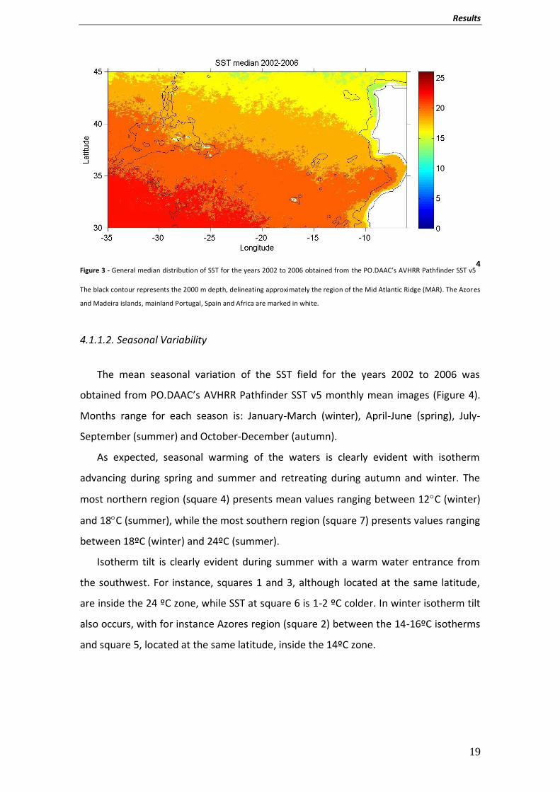
Figure 3 - General median distribution of SST for the years 2002 to 2006 obtained from the

PO.DAAC’s AVHRR Pathfinder SST v5. The black contour represents the 2000 m depth,

delineating approximately the region of the Mid Atlantic Ridge (MAR). The Azores and Madeira

islands, mainland Portugal, Spain and Africa are marked in white.

Figure 4 - Seasonal mean distribution of SST for the years 2002 to 2006 obtained from

PO.DAAC’s AVHRR Pathfinder SST v5. The black contour represents the 2000 m depth,

delineating approximately the region of the Mid Atlantic Ridge (MAR). The Azores and Madeira

v

islands, mainland Portugal, Spain and Africa are marked in white. The blue contoured squares

represent the selected regions of study (see chapter 3).

Figure 5 - Annual mean distribution of SST for the years 2002 to 2006 obtained from

PO.DAAC’s AVHRR Pathfinder SST v5. The black contour represents the 2000 m depth,

delineating approximately the region of the Mid Atlantic Ridge (MAR), the Azores and Madeira

islands, mainland Portugal, Spain and Africa. These regions are marked in white. The blue

contoured squares represent the selected regions of study (see chapter 3).

Figure 6 - General median distribution of OC for the years 2002 to 2006 obtained from the

Ocean Color Level 3 browser. The black contour represents the 2000 m depth, delineating

approximately the region of the Mid Atlantic Ridge (MAR). The Azores and Madeira islands,

mainland Portugal, Spain and Africa are marked in red.

Figure 7 - Seasonal mean distribution of OC for the years 2002 to 2006 obtained from Ocean

Color Level 3 browser. The black contour represents the 2000 m depth, delineating

approximately the region of the Mid Atlantic Ridge (MAR). The Azores and Madeira islands,

mainland Portugal, Spain and Africa are marked in red. The black contoured squares represent

the selected regions of study (see chapter 3).

Figure 8 - Annual mean distribution of OC for the years 2002 to 2006 obtained from Ocean

Color Level 3 browser. The black contour represents the 2000 m depth, delineating

approximately the region of the Mid Atlantic Ridge (MAR). The Azores and Madeira islands,

mainland Portugal, Spain and Africa are marked in red. The black contoured squares represent

the selected regions of study (see chapter 3).

Figure 9 - AVHRR SST all monthly means from 2002 to 2006 for oceanic regions.

Figure 10 - AVHRR SST all monthly means from 2002 to 2006 for coastal regions.

Figure 11 - AVHRR SST all monthly means from 2002 to 2006 for squares 1, 3 and 6.

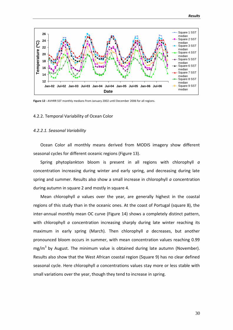
Figure 12 - AVHRR SST monthly medians from January 2002 until December 2006 for all

regions.

Figure 13 - MODIS OC all monthly means from 2002 to 2006 for oceanic regions.

Figure 14 - MODIS OC all monthly means from 2002 to 2006 for coastal regions.

vi

Figure 15 - MODIS OC monthly medians from July 2002 until December 2006 for oceanic

regions.

Figure 16 - MODIS OC monthly medians from July 2002 until December 2006 for coastal

regions.

Figure 17 - AVHRR SST and MODIS OC inter-annual monthly means from 2002 to 2006 for

square 5.

Figure 18 - AVHRR SST and MODIS OC inter-annual monthly means from 2002 to 2006 for

square 5.

Figure 19 - AVHRR SST and MODIS OC monthly medians from July 2002 until December 2006

for square 6.

Figure 20 - Correlation coefficients (K) between ∆SST monthly mean and ∆OC monthly mean

from 2002 to 2006 for southern regions.

Figure 21 - Correlation coefficients (K) between ∆SST monthly mean and ∆OC monthly mean

from 2002 to 2006 for northern regions.

Figure 22 - Correlation coefficients (K) between ∆SST monthly median and ∆OC monthly

median from 2002 to 2006 for coastal regions.

Figure 23 - SST annual mean anomaly versus annual mean NAO index from 2002 to 2006 for

the southern squares.

Figure 24 - SST anomaly annual mean and NAO index annual mean from 2002 to 2006 for

northern regions.

Abstract/Resumo

1

Abstract

Main objectives of this study are to describe temporal and spatial variability of sea

surface temperature (SST) and Ocean Color (OC) in the Subtropical Atlantic on

monthly, seasonal and inter-annual scales. As an input, five years (2002-2006) of

AVHRR SST (in ºC) (NASA/JPL/PO.DACC) and of MODIS OC (chlorophyll a in mg/ m3)

(NASA/GSFC) images were used. At the south-western part of the region, the ocean

waters were generally the warmest, while the highest OC was found at the Portuguese

coast. Result show that SST variability in the region is primarily a balance between

ocean surface heating and wind mixing, with some input of SST gradients transport by

advection. In tropical waters, inter-annual SST variability showed high negative

correlations with NAO index. With some exceptions, Ocean Color seasonal variability

varied inversely with respect to SST. In the open ocean regions spring bloom produced

the highest chlorophyll a concentration while at the Portuguese coast strong summer

bloom is present. In tropical regions, OC variability showed significant negative

correlations with SST, particularly during spring and summer.

Keywords: Northeast Subtropical Atlantic, temporal variability, sea surface

temperature, ocean color.

Resumo

Os principais objectivos deste estudo são descrever a variabilidade espacial e temporal

da temperatura de superficie do mar (SST) e da Cor do Oceano (OC) no Atlântico

Subtropical a uma escala mensal, sazonal e anual. Foram usadas cinco anos (2002-

2006) de imagens AVHRR SST (em ºC) (NASA/JPL/PO.DAAC) e MODIS OC (clorofila a em

mg/ m3) (NASA/GSFC). A parte sudoeste da região foi geralmente a mais quente

enquanto os valores mais elevados de clorofila foram encontrados na costa

portuguesa. Os resultados mostram que a variabilidade de SST na região são devido a

um balanço entre o aquecimento da superficie do oceano e a mistura causada pelo

vento. A variabilidade inter-anual de SST mostrou correlação negativa alta com o index

Abstract/Resumo

2

da NAO. Com algumas excepções a variabilidade sazonal de OC variou inversamente

no que diz respeito ao SST. Nas regiões oceanicas o bloom de Primavera produziu as

concentrações de clorofila a mais elevadas enquano que na costa portguesa ocorreu

um bloom de Verão forte. Nas regiões tropicais, e particularmente durante a

Primavera e Verão, a variabilidade de OC mostrou uma significante correlação negativa

relativamente ao SST.

Palavras chave: Atlântico Nordeste Subtropical, variabilidade temporal, temperatura

de superficie do oceano, cor do oceano.

Introduction

3

1. INTRODUCTION

The study of spatial and temporal variability of surface temperature and ocean

color patterns is of much interest for both commercial (e.g. fisheries, water quality

monitoring services) and research (e.g. atmospheric circulation/forecast models,

estimation of primary production, coupled physical-biological interactions) points of

view. For subtropical and tropical waters SST may serve as an indicator of vertical

mixing in the upper ocean layer with the lower ones. For the upper ocean layer this

mixing serves the major source of nutrients, which regulates plankton biomass and

primary productivity in the regions. Form another side, Ocean color can be regarded as

a direct measure of phytoplankton abundance and productivity in the region. There

are various approaches which permit to convert the chlorophyll a concentration,

derived from OC, to phytoplankton biomass and productivity, thus linking the former

with some of the most important biological characteristics of the ocean (Longhurst,

1995).

Sea Surface Temperature (SST) and Ocean Color (OC), measured from space,

provide an almost instantaneous large-scale view of related physical and biological

ocean patterns. Due to its global and repeated coverage, satellite-based remote

sensing offers the unique observational approach suitable for routine measurement of

physical and biological properties over large regions of the ocean (McGillicuddy et al.,

2001). The highest quality available information on the SST and OC characteristics of

the ocean can be obtained from the Advanced Very High Resolution Radiometer

(AVHRR, NOAA satellites) and Moderate Resolution Imaging Spectroradiometer

(MODIS, Aqua and Terra satellites) instruments. Previous investigations have

documented coherence between SST and OC in several different regions of the world

ocean, including the northeast Atlantic (Gower et al., 1980, Martins et al. 2007), and

the Gulf Stream (Moliner and Yoder, 1994). However, the nature of this relationship in

the subtropical gyres has received less attention (McGillicuddy et al., 2001), while joint

analysis of SST and OC can provide an insight into physical mechanisms which govern

the phytoplankton dynamics in the region.

The Azores region is characterized by rather high horizontal temperature gradients,

enhanced by two eastward flows: the cold southern branch of the North Atlantic

Current (NAC), and the warm Azores Current (AzC) (Bashmachnikov et al., 2004). The

southern branch of the NAC and the AzC are most pronounced in the eastern part of

Introduction

4

the Eastern subtropical Atlantic basin and have a slight tendency to converge towards

the Iberian Peninsula (Martins et al. 2007). This convergence enhances meridional

temperature gradients in the region. The highest horizontal temperature (1ºC per

50km) and salinity gradients in the upper layer are found in the Azores front (AzF)

(Gould, 1985). This author suggested marking the frontal interface between the

Subtropical and the North-East Atlantic Central waters at 18 ºC isotherm. The position

of the AzF and 60-km wide jet-like AzC exhibits seasonal migrations of about 3

latitude, performing a retreat towards the south in summer and progress northward in

winter (Stramma and Siedler, 1988).

Seasonal variability of phytoplankton in the region is characterized by spring

bloom, summer minimum, followed by modest autumn and winter increase.

Phytoplankton temporal and spatial variability in the region is deeply influenced by

seasonality of physical properties and water dynamics. One of the most important

regulating factors, initiating spring bloom in subtropics and winter increase in tropics is

the vertical stability of the water column. From autumn to winter, the upper mixed

layer depth deepens, favouring the entrainment of nutrient rich cold deep waters into

the photic zone. From spring to summer the picnocline strengthens, and the upper

mixed layer becomes the shallowest (10-30 m) and more effectively separated from

the ocean interior (Teira et al., 2005).

This investigation aims to study temporal and spatial variability of SST and OC in

the Eastern Subtropical Atlantic. It is based on a comparative analysis of five years of

NOAA/AVHRR and MODIS/AQUA monthly satellite imagery for 9 sub-regions. We look

for statistical dependencies between SST and OC patterns and their temporal changes

on monthly, seasonal and inter-annual time scales.

The following Section presents background information on the general dynamics of

the region and remote sensing of SST and OC. Section 3 describes the data sets and the

methodology. Section 4 presents the results. Section 5 discusses the results obtained

and section 6 presents the conclusions from this study.

Background

5

2. BACKGROUND

2.1. General Description of the Region of Study

The subtropical gyres are extensive, coherent regions that occupy about 40% of the

surface of the ocean. Once thought to be homogeneous and static habitats, there is

increasing evidence that they exhibit substantial physical and biological variability on a

variety of time scales (Mclain et al., 2004). While biological productivity within these

oligotrophic regions may be relatively small, their immense size makes their total

contribution significant (Teira et al., 2005).

The Azores archipelago is located at the northern edge of the North Atlantic

Subtropical Gyre (SG), considered to be the rotor of the North Atlantic circulation

(Bashmachnikov et al., 2004). In the Azores region, the mean currents, as well as

mesoscale motions, are comparatively weak (Lafon et al., 2004). The Gulf Stream

current feeds the Azores area, entering the region as several branches. The southern

branch is called the Azores current (AzC) and it crosses the Mid-Atlantic ridge (MAR)

between 32 and 35 ºN (Klein & Siedler, 1989). The AzC flows across the eastern basin

at approximately 34-35ºN as jet-like meandering zonal current with three main

southward recirculation branches joining at low tropics the North Equatorial Current.

The northern branch, influencing temperature variability in the region, is a southern

branch of the North Atlantic Current (NAC) that crosses MAR at 45-48 ºN

(Bashmachnikov et al., 2004).

The AzC is confined to a band of strong temperature and salinity gradients, known

as Azores Front (AzF), and forms the northern boundary of warm salty tropical waters

(Pingree et al., 1999). Stramma and Siedler (1988) reported seasonal variation in the

AzC-AzF position, which (south of the Azores) shifts to the south in summer as far as 2º

latitude. Mesoscale variability in the Azores-Madeira region is also closely related to

the meandering of the AzC-AzF system (Pingree et al., 1999).

Background

6

2.2. Definition of Remotely Observed Sea Surface Temperature

The vertical temperature structure of the uppermost ocean (~10 m) is both

complex and variable depending on the level of shear-driven ocean turbulence and the

air–sea fluxes of heat, moisture, and momentum (Emery et al., 1995; Donlon et al.,

2002). Every Sea Surface Temperature (SST) observation depends on the measurement

technique and sensor used, the vertical position of the measurement within the water

column, the local history of all component heat flux conditions, and the time of day

when the measurement was obtained. Due to all these dependences, there are

different concepts of SST. Definitions of SST provide a necessary theoretical framework

that can be used to understand the information content and relationships between

measurements of SST made by satellite and in situ.

The vertical structure of SST can be generally classified as follows (GHRSST-PP,

2007).

The interface SST (SSTint) is a theoretical temperature at the precise air-sea

interface and it represents the hypothetical temperature of the topmost layer of the

ocean water. SSTint is of no practical use because it cannot be measured using current

technology. It is important to note that it is the SSTint that interacts with the

atmosphere.

The skin SST (SSTskin) is defined as the radiometric temperature measured by

an infrared radiometer operating in the 10-12 micrometer spectral waveband. As such,

it represents the actual temperature of the water across a very small depth of

approximately 20 micrometers. This definition is chosen for consistency with the

majority of infrared satellite and ship mounted radiometer measurements. According

to Donlon et al. (2002) a strong temperature gradient is characteristically maintained

in this thin layer sustained by the magnitude and direction of the ocean–atmosphere

heat flux. SSTskin measurements are subject to a large potential diurnal cycle including

cool skin layer effects (especially at night under clear skies and low wind speed

conditions) and warm layer effects in the daytime.

The sub-skin SST (SSTsubskin) represents the temperature at the base of the

thermal skin layer where molecular and viscous heat transfer processes begin to

dominate. It is of ~1mm thick at the ocean surface. It varies on a timescale of minutes

Background

7

and may be influenced by solar warming (Donlon et al., 2002). For practical purposes,

SSTsubskin can be derived from the measurements of surface temperature by a

microwave radiometer operating in the 6-11 GHz frequency range, but the relationship

is neither direct nor invariant to changing physical conditions or to the specific

geometry of the microwave measurements.

The subsurface SST, SSTdepth, (traditionally referred to as a ‘‘bulk’’ SST) considers

any temperature within the water column beneath the SSTsubskin where turbulent heat

transfer processes dominate. It may be significantly influenced by local solar heating

and has a time scale of hours and typically varies with depth (Donlon et al., 2002).

The Foundation SST (SSTfnd) is defined as the temperature of the water column

free of diurnal temperature variability or equal to the SSTsubskin in the absence of any

diurnal signal. It is named to indicate that it is the foundation temperature from which

the growth of the diurnal thermocline develops each day. The SSTfnd product provides

an SST that is free of any diurnal variations (daytime warming or nocturnal cooling).

Only in situ contact thermometry is able to measure SSTfnd. Analysis procedures must

be used to estimate the SSTfnd from radiometric measurements of SSTskin and

SSTsubskin (GHRSST-PP, 2007).

Thus, without a clear statement of the precise depth at which the SST

measurement was made, and the circumstances surrounding the measurement, such a

sample lacks the information needed for comparison with, or validation of satellite-

derived estimates of SST using other data sources. All measurements of water

temperature, obtained from a wide variety of sensors such as drifting buoys, moored

buoys, thermosalinograph (TSG) systems, Conductivity Temperature and Depth (CTD)

systems and various expendable bathythermograph systems (XBT), are registering SST

in SSTdepth layer. In all cases, these temperature observations are distinct from those

obtained using remote sensing techniques and measurements at a given depth

arguably should be referred to as 'sea temperature' (ST) qualified by a depth in meters

rather than sea surface temperatures (Donlon et al., 2002).

Figure 1 illustrates schematically the importance of referencing the mean depth or

wavelength at which an SST measurement is determined, when it is considered upper-

ocean SST. Figure 1(a) shows the characteristic thermal structure at night or during

moderate to strong winds during the day that homogenize the temperature in the

Background

8

upper-water layers. Figure 1(b) shows the characteristic situation for late morning–

early afternoon following a period of light or absent wind and insulation. During the

day, in clear sky, calm conditions, thermal stratification of the top few meters of the

ocean will occur, resulting in significant temperature differences between SSTint,

SSTskin, SSTsubskin, and SSTdepth. Under these conditions, surface temperature deviations

greater than 3ºC, referenced to subsurface temperatures, are not uncommon and may

persist for hours (Gentemann et al., 2003). This underscores the motivation to refine

the traditional reference to bulk SST, universally used in Oceanography and

Meteorology, to the more exact parameter, SSTdepth. Since SST retrievals by satellites

are sensitive to a thin surface layer, the diurnal warming effect strongly influences

these measurements (Gentemann et al., 2003).

Figure 1 - Idealized temperature profiles of the near-surface layer (10-m depth) of the ocean during (a) nighttime and daytime

with strong wind conditions and (b) daytime low–wind speed conditions and high insolation resulting in thermal stratification of

the surface layers. (Adapted from Donlon et al. 2002)

The cloud-free conditions described by Fig. 1(b) are favorable for infrared remote

sensing of SST from satellite instruments and in such cases, the significant vertical

variation of SST demands careful attention in terms of SST data product conception,

validation, and interpretation (Donlon et al., 2002).

Background

9

In this work we will use SST in the sense of skin sea-surface temperature measured

from satellites.

2.3. Remote Sensing Measurements of SST

The integrity of all satellite-derived SST estimates is dependent of accurate

instrument prelaunch characterization and post-launch self-calibration, and may also

be limited by data processing procedures and local variations in air-sea interaction

(Brown et al, 1993). However, the quality and credibility of derived data products

depends on accounting comprehensively for the uncertainties associated with the

measurement itself, the accuracy of atmospheric correction algorithm and, the

changes within satellite sensors throughout their lifetime (Brown et al, 1993).

Since 1981, the NOAA series of polar-orbiting spacecraft have carried the Advanced

Very High Resolution Radiometer (AVHRR), an instrument with three infrared (IR)

channels suitable for estimating SST (Fox et al., 2005). These channels are located in

the wavelength regions between 3.5µm and 4µm and between 10µm and 12.5µm,

where the atmosphere is comparatively transparent (Evans and Podestá, 1998). At IR

wavelengths, the ocean surface emits radiation almost as a blackbody. In principle,

without an absorbing and emitting atmosphere between the sea surface and the

satellite, it would be possible to estimate SST using a single channel measurement. In

reality, surface-leaving infrared radiance is attenuated by the atmosphere before it

reaches a satellite sensor.

The fundamental measurement made by AVHRR sensors installed on NOAA’s

satellites is the upwelling radiance at the height of the satellite sensor specified for a

number of spectral intervals and atmospheric path-length. For views of the sea

surface, the calibrated radiance is composed of sea surface, direct atmospheric and

reflected surface radiance; therefore, it is necessary to make corrections for

atmospheric effects. Absorption and emission along the atmospheric path between

the sea surface and satellite sensor (ignoring aerosol contributions) occurs, principally,

due to water vapor, carbon dioxide, and ozone (Minnett, 1990). Among them,

absorption due to water vapour accounts for most of the needed correction (Barton et

al., 1989). Another source of error is aerosol absorption. The aerosol content in the

Background

10

atmosphere is increased during volcanic eruptions and large dust storms such as those

from the Sahara. SST measurements are derived by compensating for unwanted

radiance components reflected at the sea surface and the atmospheric attenuation of

the emitted oceanic radiance. This is achieved using a weighted combination of

spectral and view-specific radiant temperatures or ‘‘brightness temperatures’’.

The history of SST computation from AVHRR radiances is discussed at length by

(McClain et al., 1985), but, briefly, radiative transfer theory is used to correct for the

effects of the atmosphere on the observations by utilizing "windows" of the

electromagnetic spectrum where little or no atmospheric absorption occurs. Channel

radiances are transformed (through the use of the Planck function) to units of

temperature, and then compared to a-priori temperatures measured at the surface.

This comparison yields coefficients which, when applied to the global AVHRR data, give

estimates of surface temperature which have been nominally accurate to 0.3 ºC

(Vazquez et al., 1998).

2.4. Definition of Ocean Color

In the open ocean the most of colored matter near the ocean surface results from

the presence and activities of microscopic organisms that make up the base of the

marine food chain. Among these organisms, the phytoplankton alter the ocean optical

properties most effectively - the absorption coefficient, the scattering coefficient, and

the volume scattering function, - in a manner that gives rise to changes in color of the

ocean surface. The phytoplankton also alters the effective penetration of visible light

(Lewis, 1995).

Water containing phytoplankton has much more complex spectral characteristics,

because the living cells of these small plant organisms typically contain colored

pigments, as chlorophyll, used for photosynthesis. The reaction of photosynthesis uses

solar power as its energy source, thus strongly absorbs sunlight in certain parts of the

spectrum. Also detritus of dead organisms may contain skeletal material which

contributes to light scattering and light-absorbing organic matter, even though the

chlorophyll is no longer present in the dead cells. Consequently water containing

Background

11

phytoplankton has different proportions of absorbing and scattering elements

according to the species and the age of the population (Lewis, 1995).

The color of the ocean results from solar energy which is backscattered from the

ocean surface and interior. The deep blue of the open oligotrophic waters results from

the selective absorption and scattering of pure seawater, only slightly changed by

phytoplankton or other optically active substances. As one moves closer to the shore,

the consequent increase of concentration of phytoplankton changes the color from

blue to green.

Pure ocean water is transparent to blue and green wavelengths, but is strongly

absorbing at longer wavelengths. Different absorption spectra are typical for

Chromophoric Dissolved Organic Matter (CDOM) and phytoplankton pigments, such as

chlorophyll a. Chlorophyll a, the most abundant photosynthetic pigment found in

phytoplankton, has a primary absorption peak near 440 nm. CDOM absorption

monotonically increases as wavelength decreases into the ultraviolet (UV). At the same

time, scattering from water particles enhances reflectance at longer wavelengths. The

net result is a shift from blue water to brownish water as pigment and particulate

concentrations increase (McClain, 2008). The questions are whether or not changes in

the spectral reflectance are sufficiently correlated with a single pigment concentration

such as chlorophyll a to be quantitatively useful and, if that’s the case, whether or not

accurate observations of ocean reflectance could be made from a satellite so that large

areas could be surveyed rapidly and routinely.

2.5. Remote Sensing Measurements of Ocean Color

One of the first remote sensing demonstrations that the shift in spectral shape

related to chlorophyll a concentration can be instrumentally registered was done with

airborne sensor to measure the spectra of backscattered light from the sea (Clarke et

al., 1970).

Still atmospheric contribution to the total reflectance, measured by an ocean color

sensor, increases dramatically with altitude as a result of Rayleigh (gas molecules) and

aerosol scattering. In fact, at the top of the atmosphere, the radiance emanating out of

the water column contributes no more than 15% of the total outgoing radiance

Background

12

(McClain, 2008). To remove the effect of atmosphere, a correction scheme needs to

accurately account for numerous scattering (gases and aerosols), absorption (at least

ozone absorption), and surface reflection (sun glint) effects, for a wide range of solar

and sensor-viewing geometries (McClain, 2008). In 1978 NASA launched Nimbus-7

satellite carrying the first scanning radiometer, operating in visible and near-visible

wavelengths and primarily designed to observe ocean color, known as the Coastal

Zone Color Scanner (CZCS) (Robinson, 1985). The CZCS had ocean color bands at 443,

520, and 550 nm for quantifying changes in the marine spectral slope with pigment

concentration (McClain, 2008).

After the CZCS (1978–1986) demonstrated that quantitative estimations of

geophysical variables such as chlorophyll a and diffuse attenuation coefficient could be

derived from the radiances, registered at the top of the atmosphere, a number of

international missions with ocean color sensors were launched, beginning in the late

1990s. The most known examples are: the Ocean Color and Temperature Sensor

(OCTS, Japan, 1996–1997), the Sea-viewing Wide Field-of-view Sensor (SeaWiFS,

United States, 1997-present), two Moderate Resolution Imaging Spectroradiometers

(MODIS, United States, Terra/2000-present and Aqua/2002-present), the Global

Imager (GLI, Japan, 2002–2003), and the Medium Resolution Imaging Spectrometer

(MERIS, European Space Agency, 2002-present). These missions have provided data of

exceptional quality and continuity, allowing to cover a wide variety of marine research

topics (McClain, 2008).

In this investigation MODIS sensor is used to retrieve normalized water-leaving

reflectance necessary to estimate chlorophyll a concentration. The Moderate

Resolution Imaging Spectroradiometer (MODIS), a major NASA Earth observing System

(EOS) instrument, was launched aboard the Terra satellite on December 18, 1999

(10:30 AM equator crossing time, descending) for global monitoring of the

atmosphere, terrestrial ecosystems, and oceans. On May 4, 2002, a similar instrument

was launched on the EOS-Aqua satellite (1:30 PM equator crossing time, ascending).

The EOS Project is designed to collect data for 15 years in order to differentiate short-

term and long-term trends, as well as, regional and global phenomena. MODIS, with its

2330 km viewing swath width flying onboard Terra and Aqua, provides almost

complete global coverage in one day. It acquires data in 36 high spectral resolution

Background

13

bands between 0.415 and 14.235 nm with spatial resolutions of 250 m (2 bands), 500

m (5 bands), and 1000 m (29 bands) (Savtchenko et al., 2004). Ocean color sensors like

MODIS, have been used extensively in oceanographic studies to quantify the processes

responsible for the observed phytoplankton patterns. The radiance measured by

MODIS at high spatial resolution provides improved and valuable information about

the physical structure of the Earth’s atmosphere and surface (Barnes et al., 1998), and

provides a long term data set with the same geophysical parameters for the study of

climate and global change studies (Salomonson et al., 2001, Savtchenko et al., 2004).

Data Sets and Methods

14

3. DATA SETS AND METHODS

3.1. AVHRR Data

This study uses the Sea Surface Temperature (SST) satellite images obtained from

NOAA (16 and 17) Advanced Very High Resolution Radiometer (AVHRR) to study spatial

and temporal variability of SST in the NE Subtropical Atlantic. The initial images were

processed at University of Miami's Rosenstiel School of Marine and Atmospheric

Science (RSMAS) in partnership with the NOAA National Oceanographic Data Center

(NODC)1. NOAA/AVHRR derived SST values (in ºC) were obtained using the Multi-

Channel SST (MCSST) algorithm (McClain et al., 1985) and then averaged to 9-day

temporal resolution and 4 km spatial resolution. In this investigation we used monthly

means for the period January 2002 to December 2006 (a total range of sixty months),

processed by the Physical Oceanography Distributed Active Archive Center (PO.DAAC)

at the Jet Propulsion Laboratory (JPL) of the California Institute of Technology and the

National Aeronautics and Space Administration (NASA). The data are available at

PO.DAAC (2008).

To avoid the diurnal thermocline formation effect and minimize the difference

between surface skin layer and mixed layer temperature, only night time images were

used. The resulting images contained remnant errors. To improve atmospheric noise

removal the images were post-processed with a threshold filter, e.g. the SST values

less than 10ºC in the northern part of the region and for upwelling zones, and less than

12ºC for the central and southern parts of the region, were excluded from further

analyses. The threshold values for the region were chosen based on conclusions of

Lafon et al. (2004).

1. For further details about AVHRR SST data processing, validation and technical specifications please visit:

- http://podaac.jpl.nasa.gov/DATA_CATALOG/avhrrinfo.html

- http://www.rsmas.miami.edu/groups/rrsl/pathfinder/Matchups/match_index.html ;

Data Sets and Methods

15

3.2. MODIS DATA

Ocean Color (OC) images were obtained from the Moderate Resolution Imaging

Spectroradiometer (MODIS) installed on AQUA satellite. The initial images were

processed by the Ocean Data Processing System (ODPS) at NASA’s Goddard Space

Flight Center2. Chlorophyll a concentrations (in mg/m3), were obtained using the Case

1 Chlorophyll a algorithm (Carder et al., 2003), and then averaged to 9-day temporal

resolution and 4 km spatial resolution. For this study we used monthly means for the

period of July 2002 to December 2007 (the total range of fifty four months) available

from the “Ocean Color Level 3 browser” (OceanColor Web, 2008).

To improve atmospheric noise removal the images were post-processed with a

threshold filter. Values higher than 7 mg/ m3 and 20 mg/ m3 were excluded from

further analyses in oceanic and upwelling zones, respectively. Threshold values of

chlorophyll a for the region were chosen based on the work by Martins et al. (2007)

3.3. Definition of Regions

The area for this study is defined as a 15 ºx29º latitude–longitude box extending

from 30ºN to 45ºN and from 6º W to 35º W. To ensure that zones with distinct water

characteristics were covered, as well as, for further statistical analyses, nine sub-

regions, distributed over the whole area, were defined (Figure 2 and Table 1).

2.

For further details about MODIS OC data processing, validation and technical specifications please visit:

- http://oceancolor.gsfc.nasa.gov/DOCS/MODISA_processing.html ;

- http://oceancolor.gsfc.nasa.gov/VALIDATION/ ;

- http://oceancolor.gsfc.nasa.gov/DOCS/;

Data Sets and Methods

16

Figure 2 – Map of general bathymetry (m) of the region of study and selected sub-regions.

Table 1 - Geographic limits and number of pixels in each of the selected sub-regions.

Square Latitude range Longitude range No. of Pixels

1 33ºN – 35ºN 33ºW – 31ºW 2163

2 38ºN – 40ºN 29ºW – 27ºW 2128

3 33ºN – 35ºN 29ºW – 27ºW 2163

4 43ºN – 45ºN 22ºW – 20ºW 2163

5 38ºN – 40ºN 22ºW – 20ºW 2163

6 33ºN – 35ºN 22ºW – 20ºW 2163

7 30ºN – 32ºN 22ºW – 20ºW 2163

8 38ºN – 42ºN 9.5ºW - 8.5ºW 1362

9 30ºN – 32ºN 11ºW – 9ºW 1483

3.4. Temporal Scales

In this investigation, we based our results primarily on monthly and annual means.

In some cases, when seasonal means were obtained, the seasons were distinctly

defined for SST and OC. For SST, spring encompassed the months of April-June,

summer – July-September, autumn – October-December, winter – January-March.

For OC, spring encompassed the months of March-May, summer – June-August,

autumn – September-November, winter – December-February.

The reason for this seasonal choice difference results from the fact that previous

works for the region show a decalage of about one month from initiation of surface

Data Sets and Methods

17

ocean warming and phytoplankton (expressed as satellite-derived concentration of

near-surface Chl a) bloom triggering (e.g. Martins et al., 2007).

3.5. Statistic Analysis

For all study areas and for both SST and OC, statistical parameters like monthly and

annual averages, medians, and standard deviations were calculated from the monthly

images. When we needed to eliminate the seasonal cycle, monthly anomalies (∆SST

and ∆OC) were calculated using the following formulas:

∆SST = (Monthly SST median) - (inter-annual average of monthly SST median);

∆OC = (Monthly OC median) - (inter-annual average of monthly OC median).

Resulting monthly anomaly values were cross-correlated to get statistical

dependence between the parameters. Annual mean anomalies were also correlated

with the annual mean North Atlantic Oscillation (NAO) index. The corresponding

annual mean NAO indexes were calculated based on monthly mean NAO index values

obtained from the Climate Prediction Center (CPC) at NOAA’s National Center for

Environmental Prediction (NCEP) web site (Climate Prediction Center, 2008)3.

3 For further details about monthly NAO indexes calculation please visit: - http://www.cpc.ncep.noaa.gov/products/precip/CWlink/pna/nao.shtml ;

Results

18

4. RESULTS

4.1. Patterns Analysis

4.1.1. Analysis of SST Patterns

4.1.1.1. General Mean

Distribution of the SST field for the years 2002 to 2006 was obtained from annual

means PO.DAAC’s AVHRR Pathfinder SST v5 data by taking the median values in each

pixel-point of the image (Figure 3). The highest intra-annual median SST values are

observed south of 35oN, in the south-western corner of the image, where they reach

22-23ºC. The lowest SST values are characteristic at the north-eastern part of the

region and the coast of Iberian Peninsula (14-17 C). The median SST over the Azores

region is in the range of 18-21C.

Figure 3 also shows a strong latitudinal SST gradient with the median surface

temperature increasing towards south, or more precisely to the south-south-west. A

longitudinal SST gradient is also present. The zonal isotherm tilt possibly reflects an

effect of advection patterns on the SST, forcing the isotherms to deviate from the

zonal position.

At the western coast of the Iberian Peninsula SST medians are significantly lower

than in the surrounding waters, with values ranging between 14ºC and 15ºC in the

northern part and 16-17ºC to the south. This is a result of coastal upwelling,

characteristic for the region (Matzen, 2004). Similar processes occur on the West

African coast, where the mean surface temperature is in the range of 16-19ºC.

Results

19

Figure 3 - General median distribution of SST for the years 2002 to 2006 obtained from the PO.DAAC’s AVHRR Pathfinder SST v54

The black contour represents the 2000 m depth, delineating approximately the region of the Mid Atlantic Ridge (MAR). The Azores

and Madeira islands, mainland Portugal, Spain and Africa are marked in white.

4.1.1.2. Seasonal Variability

The mean seasonal variation of the SST field for the years 2002 to 2006 was

obtained from PO.DAAC’s AVHRR Pathfinder SST v5 monthly mean images (Figure 4).

Months range for each season is: January-March (winter), April-June (spring), July-

September (summer) and October-December (autumn).

As expected, seasonal warming of the waters is clearly evident with isotherm

advancing during spring and summer and retreating during autumn and winter. The

most northern region (square 4) presents mean values ranging between 12C (winter)

and 18C (summer), while the most southern region (square 7) presents values ranging

between 18ºC (winter) and 24ºC (summer).

Isotherm tilt is clearly evident during summer with a warm water entrance from

the southwest. For instance, squares 1 and 3, although located at the same latitude,

are inside the 24 ºC zone, while SST at square 6 is 1-2 ºC colder. In winter isotherm tilt

also occurs, with for instance Azores region (square 2) between the 14-16ºC isotherms

and square 5, located at the same latitude, inside the 14ºC zone.

Results

20

Figure 4 - Seasonal mean distribution of SST for the years 2002 to 2006 obtained from PO.DAAC’s AVHRR Pathfinder SST v5. The black contour represents the

2000 m depth, delineating approximately the region of the Mid Atlantic Ridge (MAR). The Azores and Madeira islands, mainland Portugal, Spain and Africa

are marked in white. The blue contoured squares represent the selected regions of study (see chapter 3).

4.1.1.3. Inter-Annual Variability

The annual mean SST fields for the years 2002 to 2006 were obtained in each point

as the medians values of the monthly mean, obtained from PO.DAAC’s AVHRR

Pathfinder SST v5 data (Figure 5). A strong latitudinal gradient and general NW/SE tilt

of isotherms is visible for all years.

Year 2004 was the warmest with a mean temperature in the Azores region (square

2) of 18ºC and with the 14ºC isotherm reaching the 45ºN over MAR. In contrast, the

year 2002 is clearly the coldest one with a mean temperature at 45ºN falling below

12ºC and the temperature over the Azores plateau (square 2) being below 16ºC.

Longitudinal annual mean gradients also change from year to year. Thus, in 2006

the isotherms stayed more or less horizontal. In 2002, oppositely, the isotherm tilt was

quite high. This year the 20ºC annual mean isotherm did not reach the 15ºW. In 2004

1 3

4

5

6

7

8

9

2

1

2

3

4

5

6

7

8

9

Results

21

warm water with a mean temperature of 22ºC extended until 20ºW zone, but north of

35N the tilt was probably the highest.

Inter-annual variability in coastal regions (squares 8 and 9) is also evident (cf.

Figure 2). In 2005 and specially 2006 there was a clear temperature increase in these

regions. In 2006, probably due to the absence of isotherms tilt, water with mean

temperatures of 18-19ºC reaches the 40ºN in the western coast of Portugal. Minimum

SST in these regions was registered during 2002 with a mean temperature of 14-15ºC

in the coast of Portugal and 16-17ºC in the West African coast.

Res

ult

s

22

Figu

re 5

- A

nn

ual

mea

n d

istr

ibu

tio

n o

f SS

T fo

r th

e ye

ars

20

02

to

20

06

ob

tain

ed f

rom

PO

.DA

AC

’s A

VH

RR

Pat

hfi

nd

er S

ST v

5.

The

bla

ck c

on

tou

r re

pre

sen

ts t

he

20

00

m d

epth

, d

elin

eati

ng

app

roxi

mat

ely

the

regi

on

of

the

Mid

Atl

anti

c R

idg

e (M

AR

), t

he

Azo

res

and

Ma

dei

ra i

slan

ds,

mai

nla

nd

Po

rtu

gal,

Spai

n a

nd

Afr

ica.

Th

ese

regi

on

s ar

e m

arke

d i

n w

hit

e. T

he

blu

e co

nto

ure

d s

qu

ares

re

pre

sen

t th

e se

lect

ed

regi

on

s o

f st

ud

y (s

ee

chap

ter

3).

2 3

4

4 5 6 7

8 9

1

2 3

4 5 6 7

8 9

4

1

2 3

5 6 7

8

9

4

1

2 3

4 6 7

8

9

5

1

2

3

4 5 6

8 9 7

4

Results

23

4.1.2. Analysis of Ocean Color Patterns

4.1.2.1. General Mean

Distribution of the OC field for the years 2002 to 2006 was obtained from NASA’s

MODIS chlorophyll annual means data by taking the median values in each pixel-point

of the image (Figure 6). The highest intra-annual median chlorophyll a values are

observed in the west coast of Portugal and Africa where values are superior to 0.5

mg/m3.In the Northeast part of the region, they reach 0.4-0.5 mg/m3. The lowest OC

values are characteristic at the south-western part of the region (<0.1 mg/m3). The

median chlorophyll over the Azores region is in the range of 0.15-0.2 mg/m3 with

slightly increased concentration near the coast of the islands.

Figure 6 also shows a general latitudinal OC gradient with median chlorophyll

increasing towards north, or more precisely to the northeast. A slight longitudinal OC

gradient is present with higher chlorophyll concentration in the eastern part.

Figure 6 - General median distribution of OC for the years 2002 to 2006 obtained from the Ocean Color Level 3 browser1

. The

black contour represents the 2000 m depth, delineating approximately the region of the Mid Atlantic Ridge (MAR). The Azores

and Madeira islands, mainland Portugal, Spain and Africa are marked in red.

1

http://oceancolor.gsfc.nasa.gov/cgi/l3;

Results

24

4.1.2.2. Seasonal Variability

The mean seasonal variation of the OC field for the years 2002 to 2006 was

obtained from NASA’s MODIS chlorophyll monthly mean images (Figure 7). Months

range for each season is: December-February (winter), March-May (spring), June-

August (summer) and September-November (autumn).

Strong OC seasonal patterns are evident in all regions, with highest chlorophyll a

concentration during springtime and lowest in summer. During spring, strong blooms

(>0.5 mg/m3) occur in the northeast part of the region. In latitudes between 36-41ºN

small winter blooms occur (0.2-0.3 mg/m3), mainly in the Azores area. During summer

and autumn, stratification of the upper layer is high and so small blooms only occur on

the northern part of the region.

Figure 7 - Seasonal mean distribution of OC for the years 2002 to 2006 obtained from Ocean Color Level 3 browser. The black contour represents the 2000 m

depth, delineating approximately the region of the Mid Atlantic Ridge (MAR). The Azores and Madeira islands, mainland Portugal, Spain and Africa are marked

in red. The black contoured squares represent the selected regions of study (see chapter 3).

Results

25

4.1.2.3. Inter-Annual Variability

The annual mean OC fields for the years 2002 to 2006 were obtained in each point

as the medians values of the monthly mean, obtained from NASA’s MODIS chlorophyll

monthly mean images (Figure 8).

Distinct OC patterns are evident in the 5 years. All years show a general tendency

for chlorophyll concentration to increase towards northern regions. In 2005 and 2006

some increased chlorophyll values are present in southern latitudes, contrasting with

year 2002 that generally presents very low values in the whole study area. During 2003

strong blooms (>0.5 mg/m3) occurred in the most northern region (square 4). In 2004

and 2005 the strongest blooms appear on the north coast of the Peninsula Iberian,

while in 2005 the highest values were found in the northeast part of the region, west

of Portugal. Annual variability is also evident in the Portuguese coast region (square 8)

where increased chlorophyll values are found in 2005 and 2006.

Res

ult

s

26

Figu

re 8

- A

nn

ual

mea

n d

istr

ibu

tio

n o

f O

C f

or

the

year

s 2

00

2 t

o 2

00

6 o

bta

ine

d f

rom

Oce

an C

olo

r Le

vel 3

bro

wse

r. T

he

bla

ck c

on

tou

r re

pre

sen

ts t

he

20

00

m d

ep

th, d

elin

eati

ng

app

roxi

mat

ely

the

regi

on

of

the

Mid

Atl

anti

c R

idg

e (M

AR

). T

he

Azo

res

and

Mad

eira

isla

nd

s, m

ain

lan

d P

ort

uga

l, Sp

ain

an

d A

fric

a ar

e m

arke

d in

red

. Th

e b

lack

co

nto

ure

d s

qu

ares

re

pre

sen

t th

e s

ele

cte

d r

egio

ns

of

stu

dy

(se

e c

ha

pte

r 3

).

Results

27

4.2. Statistics for selected regions

4.2.1. Temporal Variability of SST

4.2.1.1. Seasonal Variability

SST inter-annual monthly means derived from AVHRR imagery show similar

seasonal cycle among all oceanic regions (Figure 9). Seasonal warming and cooling of

the waters is clearly evident, with mean temperature rising during spring and summer

and falling during autumn and winter. August is the month where all regions reach a

maximum temperature value, with an exception for the most southern region (square

7), where SST reaches its maximum only in September. The amplitudes between

winter SST minimum and summer SST maximum in all regions are around 6-7ºC.

In coastal regions (square 8 and 9), the inter-annual monthly mean SST curve

(Figure 10) shows somewhat distinct pattern. The mean temperature rises during early

spring and maintains more or less stable values during summer time. In contrast with

oceanic regions typical maximum during August is not that clearly pronounced in

coastal regions. The seasonal temperature amplitudes in these regions are also lower,

of the order of 4-5ºC.

The last two Figures (9 and 10) show the highest surface temperatures during

summertime in square 1 (25.4ºC) and the lowest during winter in square 4 (13.4ºC). A

latitudinal effect seems clearly the main source for the differences observed between

SST seasonal cycles in the region. Normally, higher latitudes are characterized by lower

surface temperatures throughout a year. Another important factor, regulating the

height and the shape of seasonal cycles, is the difference between the mean

longitudes of the areas. Figure 9 shows a comparison between regions located at the

same latitude, but at different longitudes. On the graphic it is possible to see a clear

decrease in temperature as we move eastwards (from squares 1 3 6). This last

region (square 6) also presents the lowest inter-annual temperature amplitud

Results

28

Figure 9 - AVHRR SST all monthly means from 2002 to 2006 for oceanic regions.

Figure 10 - AVHRR SST all monthly means from 2002 to 2006 for coastal regions.

Figure 11 - AVHRR SST all monthly means from 2002 to 2006 for squares 1, 3 and 6.

12

14

16

18

20

22

24

26

January

February

Marc

hA

prilM

ay

JuneJuly

August

Septem

ber

Octo

ber

Novem

ber

Dec

ember

Month

Te

mp

era

ture

(ºC

)

Square 1 SST avg

Square 2 SST avg

Square 3 SST avg

Square 4 SST avg

Square 5 SST avg

Square 6 SST avg

Square 7 SST avg

12

14

16

18

20

22

24

26

January

February

Marc

hA

prilM

ayJune

July

August

Septem

ber

Octo

ber

Novem

ber

Dec

ember

Month

Te

mp

era

ture

(ºC

)

Square 8 SST avg

Square 9 SST avg

12

14

16

18

20

22

24

26

January

February

Marc

hA

prilM

ayJune

July

August

Septem

ber

Octo

ber

Novem

ber

Dec

ember

Month

Te

mp

era

ture

(ºC

)

Square 1 SST avg

Square 3 SST avg

Square 6 SST avg

Results

29

4.2.1.2. Inter-annual Variability

Monthly median SST values derived from AVHRR imagery are presented in Figure

12. IN general, a clear seasonal warming during spring and cooling during autumn is

characteristic for all the years for all the regions in study. Nevertheless, the graphic

shows distinct seasonal cycles between years with, for instance, a clear different

pattern in 2004 where more northern regions (squares 2, 4 and 5) present lower and

more stable SST values during summer and higher and more stable SST minimum

during winter. Also in 2004, the southern regions (squares 1, 3, 6 and 7) show better

SST agreement among them, than on other years. In fact, particularly during summer,

these four stations mean surface temperatures are about 2C higher than all other

regions for the same year. In Figure 12 is also possible to see that coastal regions

(squares 8 and 9), show a distinct pattern when compared with oceanic regions.

Inter-annual comparison among different regions shows square 1 as the region

with the highest SST maximum and highest SST values in summer, with the exception

of year 2003 where square 3 gets the higher value. Northern regions tend to reach

maximum SST values sooner than southern ones. During some years the time lag is

about one month. Generally, the northern regions reach their maximum in August and

southern regions in August-September. On the other hand, there is no clear tendency

for minimum SST monthly median values. Square 4 presents the lowest SST in all years

with exception of year 2005 where square 8 gets the lowest SST minimum.

Comparison of SST seasonal amplitudes for the same period shows that during the

years 2003 (2004) the highest (lowest) SST amplitude in all regions was reached, with

few exceptions, respectively. These are for example, square 4 that reached its

maximum amplitude in 2005, and the coastal regions (squares 8 and 9) that do not

have any significant inter-annual difference in amplitude.

Results

30

Figure 12 - AVHRR SST monthly medians from January 2002 until December 2006 for all regions.

4.2.2. Temporal Variability of Ocean Color

4.2.2.1. Seasonal Variability

Ocean Color all monthly means derived from MODIS imagery show different

seasonal cycles for different oceanic regions (Figure 13).

Spring phytoplankton bloom is present in all regions with chlorophyll a

concentration increasing during winter and early spring, and decreasing during late

spring and summer. Results also show a small increase in chlorophyll a concentration

during autumn in square 2 and mostly in square 4.

Mean chlorophyll a values over the year, are generally highest in the coastal

regions of this study than in the oceanic ones. At the coast of Portugal (square 8), the

inter-annual monthly mean OC curve (Figure 14) shows a completely distinct pattern,

with chlorophyll a concentration increasing sharply during late winter reaching its

maximum in early spring (March). Then chlorophyll a decreases, but another

pronounced bloom occurs in summer, with mean concentration values reaching 0.99

mg/m3 by August. The minimum value is obtained during late autumn (November).

Results also show that the West African coastal region (Square 9) has no clear defined

seasonal cycle. Here chlorophyll a concentrations values stay more or less stable with

small variations over the year, though they tend to increase in spring.

12

14

16

18

20

22

24

26

Jan-02 Jul-02 Jan-03 Jul-03 Jan-04 Jul-04 Jan-05 Jul-05 Jan-06 Jul-06

Date

Te

mp

era

ture

(ºC

)

Square 1 SST

medianSquare 2 SST

medianSquare 3 SST

medianSquare 4 SST

medianSquare 5 SST

medianSquare 6 SST

medianSquare 7 SST

medianSquare 8 SST

medianSquare 9 SST

median

Results

31

Inter-annual monthly means (Figure 13 and Figure 14) also show the highest

chlorophyll a values during springtime in square 8 (1.04 mg/m3) and lowest during

autumn in square 7(0.05 mg/m3).

As latitude increases, regions (squares 2, 4 and 5) have more pronounced spring

blooms and reach maximum chlorophyll a later in spring (May) contrasting with

southern regions early spring blooms (March).

Figure 13 - MODIS OC all monthly means from 2002 to 2006 for oceanic regions.

Figure 14 - MODIS OC all monthly means from 2002 to 2006 for coastal regions.

0

0,1

0,2

0,3

0,4

0,5

0,6

Janua

ry

Febru

ary

Mar

chApr

il

May

June

July

Aug

ust

Sep

tem

ber

Oct

ober

Nov

ember

Dec

ember

Month

Ch

loro

ph

yll

co

nc

en

tra

tio

n

(mg

/m3

)

Sq.1 Chl a avg

Sq.2 Chl a avg

Sq.3 Chl a avg

Sq.4 Chl a avg

Sq.5 Chl a avg

Sq.6 Chl a avg

Sq.7 Chl a avg

0

0,2

0,4

0,6

0,8

1

1,2

Janua

ry

Febru

ary

Mar

chApr

il

May

June

July

Aug

ust

Sep

tem

ber

Oct

ober

Nov

ember

Dec

ember

Month

Ch

loro

ph

yll

co

nc

en

tra

tio

n

(mg

/m3

)

Sq.8 Chl a avg

Sq.9 Chl a avg

Results

32

4.2.2.2. Inter-Annual Variability

Monthly mean OC values derived from MODIS imagery (Figure 15) show distinct

seasonal cycles with increase (decrease) of Chl a pigments during February-May

(August-September). In general, results for oceanic regions show highest values in

square 4 particularly during May 2003 and June 2006. The year 2004 is an exception,

with highest Chl a values in square 5. From Figure 15 it is also possible to see a clear

tendency for the northern regions (squares 2, 4 and 5) to reach maximum chlorophyll

concentration 1 or 2 months later than the southern regions (squares 1, 3, 6 and 7).

For coastal regions (squares 8 and 9), Figure 16 shows no clear chlorophyll a

pattern over the year. During 2004 the chlorophyll values at square 8 were low. Mean

chlorophyll a values in these regions are generally higher than in the open ocean

regions. This is particularly true for the coast of Portugal (square 8) where the highest

chl a value of 1.6 mg/m3 occurs in March 2003. At the same time, the minimum values

in all regions can reach 0.04 mg/m3 (September 2003 and September 2004).

Corresponding minimum value was observed only in the most southern oceanic region

(square 7).

Figure 15 - MODIS OC monthly medians from July 2002 until December 2006 for oceanic regions.

0

0,2

0,4

0,6

0,8

1

1,2

Jul-02 Jan-03 Jul-03 Jan-04 Jul-04 Jan-05 Jul-05 Jan-06 Jul-06

Date

Ch

loro

ph

yll a

co

nc

en

tra

tio

n

(mg

/m3)

Square 1 Chl a

median

Square 2 Chl a

median

Square 3 Chl a

median

Square 4 Chl a

median

Square 5 Chl a

median

Square 6 Chl a

median

Square 7 Chl a

median

Results

33

Figure 16 - MODIS OC monthly medians from July 2002 until December 2006 for coastal regions.

4.2.3. Variability of SST vs Ocean Color

4.2.3.1. Seasonal Variability

Monthly mean chlorophyll a concentrations, at seasonal time scale, show evident

general tendency to behave inversely to SST. Table 2 shows the correlation coefficients

(K) between SST and OC inter-annual monthly mean values from 2002 to 2006, for the

selected regions. Significant correlation coefficients (at 1% level of significance) were

found in all regions with exception for the most northern one (square 4) and coastal

zones (squares 8 and 9). As an illustration, Figure 17 shows the inter-annual seasonal

cycle of surface temperature and chlorophyll for square 5, where the most negative

correlations were obtained. Except the short period of the spring bloom, the curves

have clear inverse seasonal cycle. Figure 18 represents SST and chlorophyll behaviour

for the most northern region (square 4) with the least correlation between the 2

parameters. Here there is no correspondence between the curves until May and then

an inverse behaviour is observed on forward months.

Correlation coefficients between the inter-annual monthly means of SST and OC

for the spring period (March to May) were also calculated, and the results are shown in

Table 3. Despite correlations coefficients found in almost every region (except square

9) were high, only squares 1, 3, 6 and 8 were correlated at 5% level of significance. This

happens because only 3 monthly values were used for correlation calculations

between the parameters. Nevertheless, it is still possible to see a clear tendency for

0

0,2

0,4

0,6

0,8

1

1,2

1,4

1,6

1,8

Jul-02 Jan-03 Jul-03 Jan-04 Jul-04 Jan-05 Jul-05 Jan-06 Jul-06

Date

Ch

loro

ph

yll

a c

on

cen

trati

on

(mg

/m3)

Square 8 Chl

a median

Square 9 Chl

a median

Results

34

southern regions to have a higher negative correlation coefficient than northern

regions.

Table 2 - Correlation coefficients (K) between SST inter-annual monthly mean and OC inter- annual monthly mean from 2002 to

2006 for the different regions. K critical value at 5% and 1% levels of significance respectively: 0,55 and 0,68.

Square 1 2 3 4 5 6 7 8 9

K -0,87 -0,87 -0,90 -0,37 -0,94 -0,88 -0,85 -0,39 -0,53

Figure 17 - AVHRR SST and MODIS OC inter-annual monthly means from 2002 to 2006 for square 5.

Figure 18 - AVHRR SST and MODIS OC inter-annual monthly means from 2002 to 2006 for square 5.

Table 3 - Correlation coefficients (K) between SST and OC during the period of spring bloom for the different regions. Years 2002

to 2006. K critical value at 5% and 1% levels of significance respectively: 0,95 and 0,99.

0

5

10

15

20

25

January

February

Marc

hA

prilM

ay

JuneJuly

August

Septem

ber

Octo

ber

Novem

ber

Dec

ember

Month

Te

mp

era

ture

(ºC

)

0

0,05

0,1

0,15

0,2

0,25

0,3

Ch

loro

ph

yll

a

co

nc

en

tra

tio

n (

mg

/m3)

Square 5

SST avg

Sqaure 5

Chl a avg

0

5

10

15

20

25

Month

January

February

Marc

hA

prilM

ayJune

July

August

Septem

ber

Octo

ber

Novem

ber

Month

Te

mp

era

ture

(ºC

)

0

0,1

0,2

0,3

0,4

0,5

0,6

Ch

loro

ph

yll

a

co

nc

en

tra

tio

n (

mg

/m3 )

Square 4

SST avg

Sqaure 4

Chl a avg

Square 1 2 3 4 5 6 7 8 9

K -0,99 0,85 -0,99 0,86 -0,85 -0,98 -0,91 -0,97 -0,50

Results

35

4.2.3.2. Inter-Annual Variability

Monthly SST and chlorophyll a means from July 2002 to December 2006 show a

clear inverse relationship for each year of the studied period of time. As an example,

Figure 19 shows evident inverse inter-annual seasonal cycle between SST and OC for

square 6. In the graphic is also possible to see that to a comparatively high SST

minimum in 2006 corresponds the lowest chlorophyll a peak during the winter-spring

period.

In order to take out the seasonal cycle influence and enhance the inter-annual

variability, anomalies of both SST and OC were calculated on a monthly basis. SST and

OC monthly anomalies were then, independently, correlated throughout the years.

The correlation coefficients (K) for each square are shown in Figure 20, Figure 21 and

Figure 22 are graphical representations of Table 4. For better interpretation, they are

separated into southern, northern and coastal areas, respectively. In southern regions

it is possible to see a general tendency for parameters being more negatively

correlated during the spring period (February to May), and to have lower or even

positive correlation coefficients during summer, autumn and winter periods (June to

January). For northern squares no clear trend is observed, with considerable variation

of the correlation coefficients during the year and in all the squares. The coast of

Portugal (square 8) has a general tendency to present some low positive coefficient

values during winter and spring periods and negative coefficient values mainly during

autumn. In the West African coast region (square 9) stronger negative correlation

coefficients are present during spring (March to May), and autumn and winter

(September to January) periods.

0

5

10

15

20

25

Jul-02 Jan-03 Jul-03 Jan-04 Jul-04 Jan-05 Jul-05 Jan-06 Jul-06

Date

Te

mp

era

ture

(ºC

)

0

0,05

0,1

0,15

0,2

0,25

0,3

Ch

loro

ph

yll

a c

on

ce

ntr

ati

on

(mg

/m3)

Square 6 SST

median

Square Chl a

median

Results

36

Figure 19 - AVHRR SST and MODIS OC monthly medians from July 2002 until December 2006 for square 6.

Table 4 - Correlation coefficients (K) between ∆SST monthly median and ∆OC monthly median from 2002 to 2006. K critical value

at 5% and 1% levels of significance respectively: 0,81 and 0,92.

Square

1

Square

2

Square

3

Square

4

Square

5

Square

6

Square

7

Square

8

Square

9

January -0,24 -0,24 -0,99 0,56 0,38 -0,95 0,22 0,56 -0,87

February -0,97 -0,32 -0,87 0,86 -0,01 -0,75 -0,90 0,53 0,75

March -0,40 -1,00 -0,77 -0,73 0,86 -0,99 -0,90 0,81 -0,55

April -0,98 0,58 -0,96 -0,28 0,79 -0,55 -0,96 0,19 -0,77

May -0,73 -0,99 -0,94 0,43 0,81 -0,93 -0,28 0,48 -0,56

June -0,59 -0,25 -0,66 -0,93 -0,87 -0,56 -0,50 -0,08 0,29

July 0,52 0,55 -0,36 -0,36 -0,95 -0,86 -0,42 -0,13 0,38

August 0,53 0,41 -0,16 -0,79 -0,30 -0,83 -0,67 -0,69 -0,25

September 0,40 0,40 -0,50 -0,84 -0,60 0,24 -0,89 -0,20 -0,58

October -0,99 -0,83 -0,96 -0,96 -0,98 -0,52 0,30 -0,74 -0,43

November -0,81 -0,81 0,53 -0,02 -0,79 -0,88 -0,73 -0,77 -0,65

December 0,08 -0,18 0,49 0,22 0,23 -0,30 -0,86 0,76 -0,42

K Annual

mean -0,348 -0,222 -0,513 -0,237 -0,121 -0,656 -0,550 0,059 -0,305

Results

37

Figure 20 - Correlation coefficients (K) between ∆SST monthly mean and ∆OC monthly mean from 2002 to 2006 for southern

regions.

Figure 21 - Correlation coefficients (K) between ∆SST monthly mean and ∆OC monthly mean from 2002 to 2006 for northern

regions.

Figure 22 - Correlation coefficients (K) between ∆SST monthly median and ∆OC monthly median from 2002 to 2006 for coastal

regions.

-1,0

-0,8

-0,6

-0,4

-0,2

0,0

0,2

0,4

0,6

0,8

1,0

January

February

Marc

hA

prilM

ayJune

July

August

Septem

ber

Octo

ber

Novem

ber

Dec

ember

Month

Co

rrel

atio

n c

oef

ficie

nt (

K)

Square 1 K

(∆SSTvs∆Chl)

Square 3 K

(∆SSTvs∆Chl)

Square 6 K

(∆SSTvs∆Chl)

Square 7 K

(∆SSTvs∆Chl)

-1,0

-0,8

-0,6

-0,4

-0,2

0,0

0,2

0,4

0,6

0,8

1,0

January

February

Marc

hApril

May

JuneJuly

August

Septem

ber

October

November

Decem

ber

Month

Co

rrel

atio

n C

oef

ficie

nt (

K) Square 2 K

(∆SSTvs∆Chl)

Square 4 K

(∆SSTvs∆Chl)

Square 5 K

(∆SSTvs∆Chl)

-1,0

-0,8

-0,6

-0,4

-0,2

0,0

0,2

0,4

0,6

0,8

1,0

January

February

Marc

hApril

May

JuneJuly

August

Septem

ber

October

November

Decem

ber

Month

Co

rrel

atio

n c

oef

ficie

nt (

K) Square 8 K

(∆SSTvs∆Chl)

Square 9 K

(∆SSTvs∆Chl)

Results

38

4.2.4 Variability of SST vs NAO

Some attempts were made to relate part of the observed SST inter-annual

variability with the North Atlantic Oscillation (NAO). To do this, comparisons between

the annual means of SST anomaly and NAO index were made. Figure 23 shows the

results for the southern squares, where a similar pattern over the years is observed,

with a fairly good level of correspondence between these two parameters in southern

regions in 2003, 2004, 2005 and 2006. Year 2002 is somewhat different. Here high

negative SST anomaly around -0.31/-0.47 was associated with lower, but still quite

high and positive NAO index (0.04). The correspondence found between northern

regions SST anomaly and NAO indexes on annual means was not very clear (Figure 24).

For the time interval (2002-2006), the correlation coefficient between the annual

means SST anomalies and the NAO indexes was calculated. In spite of the good level of

correspondence, no data was correlated at 5% level of significance. This possibly

happens due to a very limited temporal scale, when only five annual means values

were used. The corresponding correlation coefficients are presented in Table 5.

Interestingly, the only two regions which showed a negative SST correlation with NAO

where squares 2 and 4, both at the same latitude (latitude of the Azores region)

Some attempts were made to relate OC anomalies annual mean with NAO index

annual mean, but correlations found were very low.

Results

39

Figure 23 - SST annual mean anomaly versus annual mean NAO index from 2002 to 2006 for the southern squares.

Figure 24 - SST anomaly annual mean and NAO index annual mean from 2002 to 2006 for northern regions.

Table 5 - Correlation coefficients between ∆SST anomaly annual mean and NAO index annual mean for the different regions. K

critical value at 5% and 1% levels of significance respectively: 0,81 and 0,92.

Square 1 2 3 4 5 6 7

∆SST vs NAO index correlation 0.30 -0.12 0.50 -0.62 0.03 0.74 0,75

South squares vs NAO index

-0,60

-0,40

-0,20

0,00

0,20

0,40

0,60

0,80

2002 2003 2004 2005 2006

Year

∆S

ST

(ºC

)Square 1 ∆SST avg

Square 3 ∆SST avg

Square 6 ∆SST avg

Square 7 ∆SST avg

NAO index avg

North squares vs NAO index

-0,60

-0,40

-0,20

0,00

0,20

0,40

0,60

2002 2003 2004 2005 2006

Year

∆S

ST

(ºC

)

Square 2 ∆SST avg

Square 4 ∆SST avg

Square 5 ∆SST avg

NAO index avg

Discussion

40

5. DISCUSSION

In this chapter the results on SST and OC seasonal and inter-annual variability,

obtained in the previous section, are discussed. Comparative analysis with some

known physical processes and previous studies for the area are here addressed.

5.1. Seasonal Variability

At mid-latitudes, the temperature of the mixed layer is mainly a balance between

solar heating tending to raise the temperature, and the stirring of the upper layers by

wind which tends to mix the heat downwards, reducing the surface temperature and

deepening the mixed layer (Robinson, 1985). The latent and sensible heat exchanges

with atmosphere also play an important role at certain period of time. All these

processes show strong seasonal variation, increasing from the tropics to mid-latitudes,

thus, the upper ocean layer temperature shows a pronounced seasonal cycle.

Seasonal variability of solar heating resulted in SST gradients seasonal meridional

migrations, in which enhanced SST advection during spring-summer seasons also

seems to have played an important role. Martins et al. (2007) attributed this feature to

seasonal Sub-tropical Gyre (SG) expansion. Our results also showed that for the whole

study area strong SST seasonal patterns were evident. During all seasons meridional

gradients were the most pronounced, with temperature increasing (decreasing) in

southern (northern) latitudes, respectively. In winter, the low heat input and strong

mixing by the winds results in lower temperatures and deeper upper mixed layer. In

summer, the increased insolation and generally lower wind stirring, means that the

shallow surface layer heats up, becoming thermally isolated (seasonal thermocline)

from the deeper part of what was the winter mixed layer. Previous studies in the

region also indicate that the upper layer water warming, and the associated isotherm

displacement towards north during spring and early summer, is often accompanied by

barring of the internal horizontal temperature patterns by formation of the seasonal

thermocline (Bashmachnikov et al., 2004, Martins et al., 2007).

Apart of the meridional gradients, zonal isotherm tilt occurred creating a general

SST pattern with NW-SE orientation and evident longitudinal gradients of SST during all

Discussion

41

seasons. This was especially pronounced in summer and it is probably the reason why

our westernmost region (square 1) presented the highest SST during summer. Zonal

isotherm tilt during summertime suggests strong influence of the dominating eastward

flow. Klein and Siedler (1989) found summer intensification of the eastward flow

through the Azores from CTD data. Bashmachnikov et al. (2004) suggested that the

pattern may be associated with lagged response of the Gulf Stream spring-early

summer intensification or/and local forcing mechanisms, which increase the AzC

transport in the late summer. Zonal orientation of SST gradients in the western part of

the region are also enhanced due to the blocking effect of Midle-Atlantic Ridge (MAR)

on the warm water transport to the eastern Atlantic basin (see, for example, Klein and

Siedler, 1989).

Following Gould (1985) and based on in-situ temperature data retrieved from

Argos buoys, Pingree et al. (1999) suggested associating the position of the Sub-

Tropical Azores Front (AzF) with the 18ºC isotherm during cold season. Similar to the

results of Bashmachnikov et al. (2004), our results show that, during wintertime, the

AzF if identified at the position of the 18ºC isotherm was located south of 34-35ºN.

The observed seasonal migrations of the AzC main jet (south retreat in summer and

progress northward in winter), the earlier (spring) exhibit of similar seasonal pattern of

the Gulf Stream, and the analogous seasonal variability of the North Equatorial

current, all of these reflect in fact the meridional seasonal migrations and transport

variability of the North Atlantic SG (Stramma and Siedler, 1988). The seasonal SST

variability over the Sub-Tropical NE Atlantic is sensibly affected by the transport

changes described above.

Coastal regions (squares 8 and 9) have a distinct seasonal pattern. The mean

temperature rose during early spring and kept more or less stable during summer

time. In contrast with oceanic regions, which have typical SST maximum in August, for

the coastal regions the summer maximum was not that clearly pronounced.

Nevertheless, results for west Portuguese coast (square 8) are consistent with previous

results by Matzen (2004) which registered higher surface temperature during summer

period. Oliveira et al. (2008) showed that the summer oceanographic conditions along

the west Portuguese coast are dominated by coastal upwelling driven by persistent

equatorward winds. Associated filaments, previously described by Sousa and Bricaud

Discussion

42

(1992), Matzen (2004) and Oliveira et al. (2008) propagate offshore and cause

relatively high spatial-temporal variability resulting in a wide band of cooler water at

the coast. The same authors showed that the upwelling intensity in the Portuguese

coast is maximum during the months of July-September. For the same period, Barton

et al. (1998) reported an increase of northern winds over the West African coast and

respective Canary upwelling intensification. This intensification can be seen in our

results for the West African coast (square 9), where, although having typical summer

maximum, the temperature difference with the oceanic region (square 7) is about 2ºC

in winter and 3oC in summer.

The abundance of phytoplankton in water mass is believed to represent a balance

between the processes of growth (photosynthesis) and mortality (including grazing).

The production processes are controlled mainly by the abundance of light and

nutrients. The seasonal change in growth is closely tied to the change in the depth of

the mixed layer relative to the depth of photic layer, both of which, in turn, are

regulated by climatological processes such as wind stress, air-sea temperature

exchange and changes in solar radiation intensity (Yentsch, 1993).

The chlorophyll concentration at the sea surface generally responds to the

seasonal cycle of solar heating that strongly impacts vertical stability, which regulates

the intensity of upward nutrient flux (Dandonneau et al., 2004). Results show a general

tendency of the mean chlorophyll a to decrease towards southern latitudes, where

permanently stratified oligotrophic Sub-Tropical waters are found. The dominant

scheme is a transition from a high-latitude system where the bloom is triggered by the

rapid temperature, light and vertical stability increase in spring, to a low-latitude

system where it is triggered by episodic weakening of vertical stability that allows

deeper nutrients to fuel the permanently warm, nutrient-exhausted mixed layer

(Dandonneau et al., 2004).

In the northern part of the study region (squares 2, 4 and 5) a typical mid-latitude

seasonal curve with pronounced spring (usually May) bloom is found. These blooms

happen when warmer temperature and increased sunlight, creates a pycnocline that

traps nutrients at the ocean surface. During summertime, phytoplankton uses up the

available nutrients which are gradually depleted in the upper layer due to animal’s

death and sink down to the deeper layers. In autumn, cooler days cause some vertical

Discussion

43

mixing that may bring nutrients up from below resulting in a relatively smaller fall

bloom (Martins et al., 2007). In our results, fall bloom was present only in squares 2

and 4. Once winter begins, decreasing surface temperature and frequent storms cause

heavy mixing. As phytoplankton do not remain most of the time in the photic layer, the

sunlight becomes a limiting factor and winter is characterized by relatively stable low-

biomass conditions at these latitudes (Sverdrup, 1953).

More southern regions (squares 1, 3, 6 and 7), located at the northern border of

the SG, present a different seasonal pattern with a reduced winter-spring bloom and

maximum chlorophyll a values to occur in late winter - early spring (usually March).

Here, in the more equatorward provinces of the Westerlies, the consistent feature of

the seasonal cycle is that algal biomass accumulates only during the first few months

of the progressive increase in primary production rate during winter (Longhurst, 1995).

Some months before the spring production maximum, a late winter chlorophyll

maximum is reached and biomass declines progressively towards a late summer

minimum. During the winter months, the area of the oligotrophic gyre is smaller

compared to the summer months because winter storms and stronger winter winds

increase vertical mixing in the subtropical regions (Polovina et al., 2008). At these

latitudes cooling and wind stress during autumn period is not enough to mix the water

and bring the nutrients to the strongly stratified photic layer, so no autumn bloom

occurs.

Within these oligotrophic regimes, the presence of mesoscale features such as

fronts, eddies and seamounts represents important inputs of nutrient to photic layer,

leading to increases in biological production, favoring export production and the

prevalence of short food webs. (Huskin et al., 2001). Our results showed that mean

surface chlorophyll a values for sub-tropical regions were low in summer (<0.1 mg/m3)

but increased in the cooling period reaching values of 0.25 mg/m3 in late March. Based

on cruise data near 34ºN in the Eastern Basin, Pingree et al.(1999) found very similar

surface values (<0.1 mg/m3 for summer and 0.3 mg/m3 for March). Chlorophyll spring

bloom values for square 3 are slightly higher when comparing with squares 1 and 6,

this possible reflects entrainment of northerly richer waters due to the meandering of

the AzC just west of the area. Significantly higher concentrations in temperate regions

Discussion

44

(square 4) than sub-tropical and tropical ones, was mainly due to the stronger spring

bloom, which extends from 39º to 50ºN (Longhurst, 1995 and E. Teira et al. 2005).

Coastal areas (squares 8 and 9) showed a completely distinct seasonal pattern than

the oceanic regions. At the Portuguese coast (square 8) chlorophyll a concentration

increased sharply during late winter reaching its maximum in early spring (March).

Then chlorophyll a decreased, but another pronounced bloom occurred in summer,

with mean concentration values reaching 0.99 mg/m3 by August. This pronounced

summer bloom is due to the intensification of the coastal upwelling driven by stronger

trade winds, being also more aligned with the coast. This summer bloom was

previously reported by Sousa and Bricaud (1992), and Oliveira et al. (2008). Seasonal

variability in square 9 (West African coastal region) had no clear defined seasonal

cycle, having with more or less stable chlorophyll concentration over the year (~0.4

mg/m3), although, the chlorophyll a tended to slightly increase in spring. Low mean

chlorophyll values through the whole year around ~0.5 mg/m3 with a slight spring

increase were also reported by Barton et al. (1998). The relatively small year round

variation in chlorophyll concentrations integrated over the water column contrasts

with the much larger variability in primary production. During the autumn, primary

production is as low as in the most oligotrophic regions of the world. In late winter and

early spring, however, productivity values increase more than an order of magnitude.

The seasonal increase in primary productivity is not accompanied by a similar increase

in chlorophyll accumulation. Barton et al. (1998), based on in situ chlorophyll data

together with the complete archive of CZCS images for the Canaries region, indicated

that at the start of the mixing period (January–February) only a weak bloom is

produced. It appears that grazers take advantage of the phytoplankton bloom rapidly

to prevent any surface accumulation (Arístegui, 1990 fidé Barton et al., 1998), so that

the bloom never has time to build up and then weakens into spring and summer.

Zooplankton biomass reaches its maximum a few weeks after the phytoplankton peak,

and drops sharply as the algal standing crop falls (Barton et al., 1998).

Discussion

45

5.2. Inter-Annual Variability

Over the middle and high latitudes of the Northern Hemispheric the most

prominent and recurrent pattern of atmospheric variability is the North Atlantic

Oscillation (NAO) (Talley, 1996, Hurrel et al., 2003 and Visbeck et al., 2003). Since mid-

latitude SST is mainly governed by the atmospheric forcing (Chen et al., 2002), NAO is

probably the main source of inter-annual variability of SST in the region. NAO refers to

swings in the atmospheric sea level pressure difference between the Artic (normally

Iceland) and the sub-tropical Atlantic (Azores) that is most noticeable during the boreal

cold season (November-April) and is associated with changes in the mean wind speed

and direction. Significant changes in the ocean currents and their related heat

transport are also induced by changes in the NAO (Hurrel et al., 2003). It has long been

recognized that fluctuations in SST and the strength of the NAO are related, and there

are clear indications that the North Atlantic Ocean varies significantly with the

overlying atmosphere. Visbeck et al., (2003) describe in detail the oceanic response to

NAO variability. This author suggests that the SST anomalies are driven by changes in

the surface wind and air-sea heat exchanges associated with NAO variations. The

relationship is strongest when the NAO index leads an index of the SST variability by

several weeks, which highlights the well-known result that large-scale SST over the

extra-tropical oceans responds to atmospheric forcing on monthly and seasonal time

scales (Hurrel et al., 2003).

Our results for the correlations between annual SST anomalies and annual NAO

index value for oceanic regions, show higher correlation in the southern regions

(squares 1, 3, 6 and 7) as compared with the northern ones (squares 2, 4 and 5).

Positive and increasing SST anomalies were found during the years of 2003 and 2004

responding to a slightly positive and also increasing NAO index in the same years. An

possible explanation could be related to the fact that the anticyclonic circulation

intensity of the Sub-Tropical Gyre (SG) is also correlated with NAO variations (Hurrel et

al., 2003). When the NAO index is positive, enhanced westerly flow across the North

Atlantic forces clockwise intensification of the SG around the sub-tropical Atlantic high-

pressure center (Hurrel et al., 2003), which brings warmer water to the region from

the Western Atlantic basin. The enhanced surface winds also promote an accumulation

Discussion

46

of warmer surface waters in the SG, which can also enhance the positive correlations.

Since the southern squares are located in the sub-tropical region they get much

stronger signal from variations in the NAO index.

NAO variability influences abundance, biomass, distribution, growth rates and

survival rates of the organisms (Drinkwater et al., 2003). The impacts of NAO are

generally mediated through local changes in the physical environment, such as winds,

ocean temperatures and circulation patterns (Drinkwater et al., 2003). It is known that

inter-annual variability of both phytoplankton and zooplankton reflects changes in

winds and ocean temperatures. Given the importance of vertical mixing and

stratification in both timing of the spring bloom and the succession of the

phytoplankton species, it is expected that NAO might be linked to inter-annual

variability in primary production through its relationship to winds and air temperatures

(Drinkwater et al., 2003). It is important to notice that the biology is not responding

directly to the NAO but rather indirectly through changes in the local physical or

chemical characteristics of the water that are themselves associated with variability in

the NAO.

Conclusions

47

6. CONCLUSIONS

Main objectives of this work were to study temporal and spatial variability of SST

and OC in the Sub-tropical NE Atlantic, and to find statistical dependencies between

their patterns and sign of their temporal changes on monthly, seasonal and inter-

annual scales. For a period of five years, AVHRR (SST) and MODIS (OC) monthly data

obtained from the Physical Oceanography Distributed Active Archive Center (PO.DAAC)

and “Ocean Color Level 3 browser” respectively, was used to compute seasonal and

annual medians within the study area. For further statistical analysis, nine sub-regions,

distributed over the whole area, were defined.

Results for the SST field suggest distinct inter-annual seasonal cycle with seasonal

warming clearly evident in all regions initiating during winter-spring and cooling during

summer-autumn months. Isotherm tilt during summer period should be related with

the stabilizing of the Azores Anti-cyclone in the south-western part of the region,

creating a strong and stable thermocline. Stronger advection of warm waters from

Sargasso Sea in summer is adding to a related SST increase. NOAA Wind data shows

that Trade Winds in sub-region 7 are increasing during summer, this is probably the

reason why this region gets lower SST values during this season reaching a maximum

late in September.

Coastal regions showed somewhat distinct seasonal pattern. Seasonal temperature

amplitudes were lower because despite the increase in solar hitting during summer,

the wind related intensification of the coastal upwelling did not permitted a significant

temperature increase.

Results also show that chlorophyll a, generally decreased towards southern

latitudes, resulting from a gradual transition from more productive Eastern North

Atlantic waters to stratified oligotrophic tropical waters. The OC field suggested

distinct seasonal cycle with a transition from a mid-latitude system with pronounced

spring bloom triggered by formation of seasonal thermocline, to a tropical system

where the bloom it is triggered, in late winter, by less vertical stability in the upper

layer allowing deeper nutrients to fuel the permanently warm and nutrient-exhausted

mixed layer. Sub-tropical sub-regions 2 and 5 had higher inter-annual variability and

seemed to be more sensible to weather conditions. Comparing to oceanic regions, the

Conclusions

48

coastal ones presented higher mean chlorophyll values and, at the coast of Portugal a

strong summer bloom was present, this was mainly due to intensification of coastal

upwelling as a result of increase in Trade Wind speed in summer. At the West African

coast chlorophyll a concentration stayed more a less stable over the whole year.

A clear inverse relationship between surface temperatures and chlorophyll a

distributions was found in subtropical and tropical regions. Increased pigment

concentration is generally associated with lower temperature values. The relationship

was not pronounced in most northern and coastal regions. In square 4 there was no

winter chlorophyll increase so this means that the winter mixing has a negative effect

here. SST and OC in tropical regions have higher negative correlation during spring and

summer suggesting that the dependencies change with seasons.

Results show that, on inter-annual time scales, NAO has some influence over the

physical processes in the tropical area. Particularly we found strong negative

correlations between SST and NAO index.

In conclusion, coupled inter-annual and seasonal variability are clearly highlighted

in the SST and OC imagery, providing relevant information to study ocean dynamics

variability within the Sub-Tropical NE Atlantic. Our study shows that intensity of wind

mixing has an important impact on the chlorophyll concentration in the region.

However, for a better understanding of regional to large scale influences in the region,

it is important that further studies combining multi-sensor data sets from different

satellites and in situ data are made.

Acknowledgements

49

7. ACKNOWLEDGEMENTS

I am very grateful to my advisors, Dr. Igor Bashmachnikov and Prof. Ana Martins for

all their attention and dedication. In particular, I would like to thank Dr.

Bashmachnikov for the great help it gave me along the way, through interesting

physical oceanography lessons, and also by initiating me on MatLab programming,

providing me the initial programs framework for this work.

I am thankful to Prof. João Gonçalves, Dr. Igor Bashmachnikov, Prof. Ana Martins

and Dr. Paolo Lambardi for accepting to become part of my dissertation committee.

I am grateful to all my colleagues at the Section of Oceanography at the

Department of Oceanography and Fisheries (DOP/UAç) for all the help they gave me

during the development of this research. In particular, I would like to thank Guilherme

Lopes for the great help on improving initial MatLab programs.

I thank the PO.DAAC and MODIS Ocean Color Web centers for providing freely on

the web the data sets used in this study.

I thank the staff at the University of the Azores and in particular at the Department

of Oceanography and Fisheries (DOP/UAç) for their administrative and logistic help

along the way.

Computer resources and facilities were provided by the Department of

Oceanography and Fisheries at the University of the Azores. This support is greatly

acknowledged.

I am very much grateful to all my family and friends for all their support along the

way. In particular I want to thank my university friends: Adriano, Cátia, Clara, Joana,

Laura, Margarida, Nuno, Parra, Paulo, Pedro, Tiago and Tiago Caroxo.

Above all, I want to thank Ana.

References

50

8. REFERENCES

Barnes, W. L., T. S. Pagano & V. Salomonson, 1998: Prelaunch characteristics of the

moderate resolution imaging spectroradiometer (MODIS) on EOS-AMI. IEEE Trans.

Geosci. Remote Sensing, 36 (4), 1088–1100.

Barton, I. J. & R. P. Cechet, 1989: Comparison and optimization of AVHRR sea surface

temperature algorithms. Journal of Atmospheric and Oceanic Technology 6, 1083–

1089.

Barton, E.D., J. Arístegui, P. Tett, M. Cantón, J. Garcı´a-Braune, S. Hernández-León, L.

Nykjaer, C. Almeida, J. Almunia, S. Ballesteros, G. Basterretxea, J. Escánez, L.

García-Weill, A. Herna´ndez-Guerra, F. López-Laatzen, R. Molina, M.F. Montero, E.

Navarro-Pérez, J.M. Rodríguez, K. van Lenning, H. Vélez & K. Wild, 1998: The

transition zone of the Canary Current upwelling region. Progress in Oceanography,

41, 455–504.

Bashmachnikov,I., V. Lafon & A. Martins, 2004: Sea surface Temperature Distribution

in the Azores Region. Part II: Space-Time Variability and Underlying Mechanisms.

Arquipélago. Life and Marine Sciences, 21A, 19-32.

Brown, J. W., O. B. Brown & R. H. Evans, 1993: Calibration of AVHRR Infrared channels:

a new approach to non-linear correction, Journal of Geophysical Research, 98

(NC10), 18257-18268.

Clarke G. L., G. C. Ewing & C. J. Lorenzen, 1970: Spectra of backscattered light from sea

obtained from aircraft as a measure of chlorophyll concentration. Science, 16,

1119–21.

Dandonneau, Y., P. I. Deschamps, J. M. Nicolas, H. Loisel, J. Blanchot, Y. Montel, F.

Thieuleux & G. Bécu, 2004 : Seasonal and interannual variability of ocean color and

References

51

composition of phytoplankton communities in the North Atlantic, equatorial Pacific

and South Pacific. Deep-Sea Research II, 51, 303–318.

Donlon, C. J., P. J. Minett, C. Gentemann, T. J. Nightingale, I. J. Barton, B. Ward & M. J.

Murray, 2002: Toward Improved Validation of Satellite Sea Surface Skin

Temperature Measurements for Climate Research. Journal of Climate, 15, 353-369.

Drinkwater, K. F., A. Belgrano, A. Borja, A. Conversi, M. Edwards, C. H. Greene, G.

Ottersen, A. J. Pershing & H. Walker, 2003: The response of Marine Ecosystems to

Climate Variability Associated With the North Atlantic Oscillation In: The North

Atlantic Oscillation: Climatic Significance and Environmental Impact. American

Geophysical Union, 134.

Emery, W. J., G. A. Wick & P. Schluessel. 1995: Skin and Bulk Sea Surface

Temperatures: Satellite Measurement and Corrections In: M. Ikeda and F. W.

Dobson. Oceanographic Applications of Remote Sensing.

Emery, W. J., S. Castro, G. A. Wick, P. Schluessel & C. J. Donlon, 2001: Estimating Sea

Surface Temperature From Infrared Satellite and In situ Temperature Data. Bulletin

of the American Meteorological Society, 82, 12, 2773-2786

Evans, R. & G. Podestá, 1998: Pathfinder Sea Surface Temperature Algorithm.

University of Miami, Rosenstiel, School of Marine and Atmospheric Science.

Fox, M. F., D. R. Kester & J. A. Yoder, 2005: Spatial and Temporal Distributions of

Surface Temperature and Chlorophyll in the Gulf of Maine During 1998 Using

SeaWiFS and AVHRR Imagery. Marine Chemistry, 97, 104-123.

Gentemann, C. L., C. J. Donlon, A. S. Meneth & F. J. Wentz, 2003: Diurnal signals in

satellite sea surface temperature measurements. Geophysical research letters, 30,

(N3): 1140.

References

52

Gould, W. J., 1985: Physical oceanography of the Azores front. Progress in

Oceanography, 14, 167-190.

Gower, J., K. L. Denman & R. J. Holyer, 1980: Phytoplankton patchiness indicates the

fluctuation spectrum of mesoscale oceanic structure. Nature, 288, 157-159.

Hurrel, J. W., Y. Kushnir, G. Ottersen & M. Visbeck, 2003: An Overview of the North

Atlantic Oscillation. Geophysical Monograph, 134, 10.1029/134GM01.

Huskin, I., R. Anadón, G. Medina, R. N. Head & R. P. Harris, 2001: Mesozooplankton

distribution and copepod grazing in the Subtropical Atlantic near the Azores:

Influence of mesoscale structures. Journal of Plankton research, 23, 7, 671-691.

Klein, B. & G. Siedler, 1989: On the origin of the Azores current. Journal of Geophysical

Reseach, 94 (C5), 6159-6168.

Lafon, V., A. Martins, M. Figueiredo, M. A. Melo Rodrigues, I. Bashmachnikov, A.

Mendonça, L. Macedo & N. Goulart, 2004: Sea Surface Temperature Distribution in

the Azores Region. Part: I: AVHRR Imagery and In Situ Data Processing.

Arquipélago. Life and Marine Sciences, 21A, 1-18.

Lewis, M. R., 1995: Coastal Zone Color Scanner on Nimbus and Sea-Viewing Wide Field-

of-View Sensor on Seastar In: M. Ikeda and F. W. Dobson. Oceanographic

Applications of Remote Sensing.

Longhurst, A.R., 1995: Seasonal Cycles of Pelagic Production and Consumption.

Progress in Oceanography, 36, 2, 77-167.

Martins, A. M., A. S. B. Amorim, M. P. Figueiredo, R. J. Sousa, A. Mendonça,

I.Bashmachnikov & D. S. Carvalho, 2007: Sea Surface Temperature (AVHRR, MODIS)

and Ocean Colour (MODIS) seasonal and interannual variability in the

References

53

Macaronesian islands of Azores, Madeira, and Canaries. Proceedings of SPIE, 6743,

15.

Matzen, J., 2004: Caracterização qualitative do fenómeno de afloramento costeiro de

Verão na Região de Aveiro. Universidade de Aveiro, departamento de Física.

158pp.

McClain, C. R., 2008: A Decade of Satellite Ocean Color Observations. Annual Review of

Marine Science, 1, 19-42.

McClain, E. P., W. G. Pichel & C. C. Walton, 1985: Comparative performance AVHRR-

based multichannel sea surface temperatures, Journal of Geophysical Research, 90,

11,587-11,601.

McClain, C. R., S. R. Signorini & J. R. Christian, 2004: Subtropical gyre variability

observed by ocean-color satellites, Deep Sea Research, Part II, 51, 281– 301.

McGillicuddy, D. J., V. K. Kosnyrev, J. P. Ryan & J. A. Yoder, 2001: Covariation of

mesoscale ocean color and sea-surface temperature patterns in the Sargasso Sea.

Deep-Sea Research II, 48, 1823-1836.

Minnett, P. J. 1990: The regional optimization of infrared measurements of sea-surface

temperature from space. Journal of Geophysical Research, 95, 13 497–13 510.

Moliner, G. G. & J. A. Yoder, 1994: Variability in pigment concentration in warm-core

rings as determined by coastal zone color scanner satellite imagery from the Mid-

Atlantic Bight. Journal of Geophysical Research. 99, 14277-14290.

Oliveira, P. B., R. Nolasco, J. Dubert, T. Moita & A. Peliz, 2008: Surface temperature,

chlorophyll and advection patterns during a summer upwelling event off central

Portugal. Continental Shelf Research, in press.

References

54

Pingree, R.D., C. Garcia-Soto & B. Sinha, 1999: Position and structure of the

Subtropical/Azores front region from combined Lagrangian and remote sensing

(IR/altimiter/SeaWiFS)measurements. Journal of the Marine Biological Association

of the UK, 79, 769-792.

Polovina, J. J., E. A. Howell & M. Abecassis, 2008: Ocean’s least productive waters are

expanding. Geophys. Res. Lett. 35,L03618.

Robinson, I. S., 1985: Visible wavelength “ocean-colour” sensors In: Ellis Horwood

limited. Satellite Oceanography: an introduction for oceanographers and remote-

sensing scientists.

Salomonson, V., B. Guenther & E. Masuoka, 2001: A summary of the status of the EOS

Terra Mission Moderate Resolution Imaging Spectroradiometer (MODIS) and

attendant data product development after one year of on-orbit performance.

Proceedings of the International Geoscience and Remote Sensing Symposium/

IGARSS’2001, Sydney, Australia, 9–13.

Savtchenko, A., D. Ouzounov, S. Ahmad, J. Acker, G. Leptoukh, J. Koziana & D. Nickless,

2004: Terra and Aqua MODIS products available from NASA GES DAAC. Advances in

space Research, 34, 710-714.

Sousa, F. M. & A. Bricaud, 1992: Satellite-Derived Phytoplankton Pigment Structures in

the Portuguese Upwelling Area. Journal of Geophysical research, 97, c7, 11343-

11356.

Stramma, L. & G. Siedler, 1988: Seasonal changes in the North Atlantic subtropical

gyre. Journal of Geophysical Research, 93 (C7): 8111-8118.

Sverdrup, H. U., 1953: On the conditions for the vernal blooming of phytoplankton.

Journal du Conseil Perm. International pour l’Exploration de la Mer, 18, 287-295.

References

55

Talley, L. D., 1996: North Atlantic circulation and variability, reviewed for the CNLS

conference. Physica D, 98, 625-646.

Teira, E., B. Mouriño, E. Marañón, V. Pérez, M. J. Pazó, P. Serret, D. de Armas, J.

Escánez, E. M. Woodward & E. Fernández, 2005: Variability of chlorophyll and

primary production in the Eastern North Atlantic Subtropical Gyre: potential factors

affecting phytoplankton activity. Deep-Sea Research I, 52, 569–588.

Vazquez, J., E. Kearns & K. Casey, 1998: NOAA/NASA AVHRR Oceans Pathfinder Sea

Surface Temperature Data Set User's Reference Manual Version 4.0. JPL

Publication, D-14070

Visbeck, M., E. P. Chassignet, R. G. Curry, T. L. Delworth, R. R. Dickson & G. Krahmann,

2003: The ocean’s Response to North Atlantic Oscillation Variability In: The North

Atlantic Oscillation, Climate Significance and Environmental Impact.

Yentsch, C. S., 1993: CZCS: Its role in the study of growth of oceanic phytoplankton In:

Ocean Colour: Theory an Applications in a Decade of CZCS Experience, Kluwer

Academic Publishers.

Electronic Reference

Climate Prediction Center, 2008: North Atlantic Oscillation. In:

http://www.cpc.ncep.noaa.gov/products/precip/CWlink/pna/nao.shtml (Last

access October 21, 2008);

GHRSST-PP, 2005: Understanding Sea Surface Temperature. In: http://ghrsst-

pp.metoffice.com/pages/sst_definitions/ (Last accessed June 13, 2008).

References

56

PODAAC, Physical Oceanography DAAC, 2008: Mission In:

http://podaac.jpl.nasa.gov/DATA_CATALOG/avhrrinfo.html (Last accessed May 25,

2008).

AVHRR Pathfinder Oceans, 2000: Matchup Database 1985-1997 (Version 19.0). In:

http://www.rsmas.miami.edu/groups/rrsl/pathfinder/Matchups/match_index.htm

l (Las access September 3, 2008).

Ocean Color Documents, 2008: Overview of MODIS Aqua Data Processing and

Distribution. In: http://oceancolor.gsfc.nasa.gov/DOCS/MODISA_processing.html

(Last access September 9, 2008).