Embed Size (px)
Citation preview
Living Rev Relativ (2018) 21:4 https://doi.org/10.1007/s41114-018-0013-8
REVIEW ARTICLE
Relativistic dynamics and extreme mass ratio inspirals
Pau Amaro-Seoane1,2,3,4
Received: 13 July 2017 / Accepted: 16 February 2018© The Author(s) 2018
Abstract It is now well-established that a dark, compact object, very likely a massiveblack hole (MBH) of around four million solar masses is lurking at the centre of theMilky Way. While a consensus is emerging about the origin and growth of supermas-sive black holes (with masses larger than a billion solar masses), MBHs with smallermasses, such as the one in our galactic centre, remain understudied and enigmatic. Thekey to understanding these holes—how some of them grow by orders of magnitude inmass—lies in understanding the dynamics of the stars in the galactic neighbourhood.Stars interact with the central MBH primarily through their gradual inspiral due to theemission of gravitational radiation. Also stars produce gases which will subsequentlybe accreted by the MBH through collisions and disruptions brought about by the strongcentral tidal field. Such processes can contribute significantly to the mass of the MBHand progress in understanding them requires theoretical work in preparation for futuregravitational radiation millihertz missions and X-ray observatories. In particular, aunique probe of these regions is the gravitational radiation that is emitted by somecompact stars very close to the black holes and which could be surveyed by a milli-hertz gravitational-wave interferometer scrutinizing the range of masses fundamentalto understanding the origin and growth of supermassive black holes. By extracting
B Pau [email protected]
1 Institute of Space Sciences (ICE, CSIC), Institut d’Estudis Espacials de Catalunya (IEEC)at Campus UAB, Carrer de Can Magrans s/n, 08193 Barcelona, Spain
2 Institute of Applied Mathematics, Academy of Mathematics and Systems Science, CAS,Beijing 100190, China
3 Kavli Institute for Astronomy and Astrophysics, Beijing 100871, China
4 Zentrum für Astronomie und Astrophysik, TU Berlin, Hardenbergstraße 36, 10623 Berlin,Germany
123
4 Page 2 of 150 P. Amaro-Seoane
the information carried by the gravitational radiation, we can determine the mass andspin of the central MBH with unprecedented precision and we can determine how theholes “eat” stars that happen to be near them.
Keywords Black holes · Gravitational waves · Stellar dynamics
Glossary
1 M� 1 solar mass = 1.99 × 1030 kgM• Mass of super- or massive black hole1 pc 1 parsec ≈ 3.09 × 10¹⁶ m1 Myr/Gyr One million/billion yearsAGN Active galactic nucleusBH Black holeCO Compact object (a white dwarf or a neutron star), or a stellar-
mass black hole. In general, a collapsed star with a mass ∈[1.4, 10] M� in this work
DCO Dark compact objectDF Dynamical frictionEMRI Extreme mass ratio inspiralGC Galactic centreGPU Graphics processing unitGW/GWs Gravitational wave/sHB Giant stars in the horizontal branchHST Hubble space telescopeIMBH Intermediate-mass black hole (M ∈ [102, 105] M�)IMF Initial mass functionIMRI Intermediate mass ratio inspiralLISA Laser interferometer space antennaLSO Last stable orbitMBH Massive black hole (M ≈ 106M�)MC Monte carloMW Milky WayNB6 Direct-summation N -body6NS Neutron starPN Post-NewtonianRG Red giantRMS Root mean squareSMBH Super massive black hole (M > 106M�)SNR Signal-to-noise ratioSPH Smoothed particle hydronamicsTDE Tidal disruption eventUCD Ultra-compact dwarf galaxyz Redshift
123
Relativistic dynamics and extreme mass ratio inspirals Page 3 of 150 4
Contents
Foreword . . . . . . . . . . . . . . . . . . . . . . . . . . . . . . . . . . . . . . . . . . . . . . . . . .1 Massive dark objects in galactic nuclei . . . . . . . . . . . . . . . . . . . . . . . . . . . . . . . . .
1.1 Active galactic nuclei . . . . . . . . . . . . . . . . . . . . . . . . . . . . . . . . . . . . . . . .1.2 Massive black holes and their possible progenitors . . . . . . . . . . . . . . . . . . . . . . . . .1.3 Tidal disruptions . . . . . . . . . . . . . . . . . . . . . . . . . . . . . . . . . . . . . . . . . . .1.4 Extreme mass ratio inspirals . . . . . . . . . . . . . . . . . . . . . . . . . . . . . . . . . . . .
2 GWs as a probe to stellar dynamics and the cosmic growth of SMBHs . . . . . . . . . . . . . . . . .2.1 GWs and stellar dynamics . . . . . . . . . . . . . . . . . . . . . . . . . . . . . . . . . . . . . .2.2 The mystery of the growth of MBHs . . . . . . . . . . . . . . . . . . . . . . . . . . . . . . . .2.3 A magnifying glass . . . . . . . . . . . . . . . . . . . . . . . . . . . . . . . . . . . . . . . . .
2.3.1 A problem of ∼ 10 orders of magnitude . . . . . . . . . . . . . . . . . . . . . . . . . . .2.4 How stars distribute around MBHs in galactic nuclei . . . . . . . . . . . . . . . . . . . . . . . .
3 A taxonomy of orbits in galactic nuclei . . . . . . . . . . . . . . . . . . . . . . . . . . . . . . . . .3.1 Spherical potentials . . . . . . . . . . . . . . . . . . . . . . . . . . . . . . . . . . . . . . . . .3.2 Non-spherical potentials . . . . . . . . . . . . . . . . . . . . . . . . . . . . . . . . . . . . . .
4 Two-body relaxation in galactic nuclei . . . . . . . . . . . . . . . . . . . . . . . . . . . . . . . . .4.1 Introduction . . . . . . . . . . . . . . . . . . . . . . . . . . . . . . . . . . . . . . . . . . . . .4.2 Two-body relaxation . . . . . . . . . . . . . . . . . . . . . . . . . . . . . . . . . . . . . . . .4.3 Dynamical friction . . . . . . . . . . . . . . . . . . . . . . . . . . . . . . . . . . . . . . . . .4.4 The difussion and loss-cone angles . . . . . . . . . . . . . . . . . . . . . . . . . . . . . . . . .
5 “Standard” mass segregation . . . . . . . . . . . . . . . . . . . . . . . . . . . . . . . . . . . . . . .5.1 Introduction . . . . . . . . . . . . . . . . . . . . . . . . . . . . . . . . . . . . . . . . . . . . .5.2 Single-mass clusters . . . . . . . . . . . . . . . . . . . . . . . . . . . . . . . . . . . . . . . . .5.3 Mass segregation in two mass-component clusters . . . . . . . . . . . . . . . . . . . . . . . . .5.4 Clusters with a broader mass spectrum with no MBH . . . . . . . . . . . . . . . . . . . . . . .5.5 Core-collapse evolution . . . . . . . . . . . . . . . . . . . . . . . . . . . . . . . . . . . . . . .5.6 Clusters with a broader mass spectrum with a MBH . . . . . . . . . . . . . . . . . . . . . . . .
6 Two-body extreme mass ratio inspirals . . . . . . . . . . . . . . . . . . . . . . . . . . . . . . . . .6.1 A hidden stellar population in galactic nuclei . . . . . . . . . . . . . . . . . . . . . . . . . . . .6.2 Fundamentals of EMRIs . . . . . . . . . . . . . . . . . . . . . . . . . . . . . . . . . . . . . .6.3 Orbital evolution due to emission of gravitational waves . . . . . . . . . . . . . . . . . . . . . .6.4 Decoupling from dynamics into the relativistic regime . . . . . . . . . . . . . . . . . . . . . . .
7 Beyond the standard model of two-body relaxation . . . . . . . . . . . . . . . . . . . . . . . . . . .7.1 The standard picture . . . . . . . . . . . . . . . . . . . . . . . . . . . . . . . . . . . . . . . . .7.2 Coherent or resonant relaxation . . . . . . . . . . . . . . . . . . . . . . . . . . . . . . . . . . .7.3 Strong mass segregation . . . . . . . . . . . . . . . . . . . . . . . . . . . . . . . . . . . . . . .7.4 The cusp at the Galactic Centre . . . . . . . . . . . . . . . . . . . . . . . . . . . . . . . . . . .7.5 Tidal separation of binaries . . . . . . . . . . . . . . . . . . . . . . . . . . . . . . . . . . . . .7.6 A barrier for captures ignored by rotating MBHs . . . . . . . . . . . . . . . . . . . . . . . . . .7.7 Extended stars EMRIs . . . . . . . . . . . . . . . . . . . . . . . . . . . . . . . . . . . . . . . .7.8 The butterfly effect . . . . . . . . . . . . . . . . . . . . . . . . . . . . . . . . . . . . . . . . .7.9 Role of the gas . . . . . . . . . . . . . . . . . . . . . . . . . . . . . . . . . . . . . . . . . . . .
8 Integration of dense stellar systems and EMRIs . . . . . . . . . . . . . . . . . . . . . . . . . . . . .8.1 Introduction . . . . . . . . . . . . . . . . . . . . . . . . . . . . . . . . . . . . . . . . . . . . .8.2 The Fokker–Planck approach . . . . . . . . . . . . . . . . . . . . . . . . . . . . . . . . . . . .8.3 Moment models . . . . . . . . . . . . . . . . . . . . . . . . . . . . . . . . . . . . . . . . . . .
8.3.1 Equation of continuity . . . . . . . . . . . . . . . . . . . . . . . . . . . . . . . . . . . .8.3.2 Momentum balance equation . . . . . . . . . . . . . . . . . . . . . . . . . . . . . . . . .8.3.3 Radial energy equation . . . . . . . . . . . . . . . . . . . . . . . . . . . . . . . . . . . .8.3.4 Tangential energy equation . . . . . . . . . . . . . . . . . . . . . . . . . . . . . . . . . .
8.4 Solving conducting, self-gravitating gas spheres . . . . . . . . . . . . . . . . . . . . . . . . . .8.5 The local approximation . . . . . . . . . . . . . . . . . . . . . . . . . . . . . . . . . . . . . .8.6 Monte Carlo codes . . . . . . . . . . . . . . . . . . . . . . . . . . . . . . . . . . . . . . . . .8.7 Applications of Monte Carlo and Fokker–Planck simulations to the EMRI problem . . . . . . .8.8 Direct-summation N -body codes . . . . . . . . . . . . . . . . . . . . . . . . . . . . . . . . . .
123

4 Page 4 of 150 P. Amaro-Seoane
8.8.1 Relativistic corrections: the post-Newtonian approach . . . . . . . . . . . . . . . . . . . .8.8.2 Relativistic corrections: a geodesic solver . . . . . . . . . . . . . . . . . . . . . . . . . .8.8.3 N -body units and conversion . . . . . . . . . . . . . . . . . . . . . . . . . . . . . . . . .
A Comment on the use of the Ancient Greek word barathron and bathron to refer to a black hole . . . .References . . . . . . . . . . . . . . . . . . . . . . . . . . . . . . . . . . . . . . . . . . . . . . . . . .
Foreword
The volume where capture orbits are produced is so small in comparison to othertypical length scales of interest in astrodynamics that it has usually been seen asunimportant and irrelevant to the global dynamical evolution of the system. The onlyexception has been the tidal disruption of stars by massive black holes. Only when ittranspired that the slow, adiabatic inspiral of compact objects onto massive black holesprovides us with valuable information, did astrophysicists start to address the questionin more detail. Since the problem of EMRIs (extreme mass ratio inspiral) startedto draw our attention, there has been a notable progress in answering fundamentalquestions of stellar dynamics. The discoveries have been numerous and some of themremain puzzling. The field is developing very quickly and we are making importantbreakthroughs even before a millihertz mission flies.
When I was approached and asked to write this review, I was glad to accept itwithout realising the dimensions of the task. I was told that it should be similar to aplenary talk for a wide audience. I have a personal problem with instructions like this.I remember that when I was nine years old, our Spanish teacher asked us to summarisea story we had read together in class. I asked her to define “summarise”, because Icould easily produce a summary of one, two or fifty pages, depending on what shewas actually expecting from us. She was confused and I never got a clear answer. Shereplied that “A summary is a summary and that’s it”. On this occasion, I am afraid thatI have run into the same snag and I have gone for the many-pages approach, to be surethat any newcomer will have a good overview of the subject, with relevant references,in a single document. If the document is too long, please address your complains toher, because she is solely responsible.
However, I would like to note that I have not focused on gathering as much infor-mation as possible from different sources. I think it is more interesting for the reader,though harder for the writer, to have a consistent document. This can be done by intro-ducing the subject step by step, rather than working out a compendium of citationsof the related literature. For instance, I present results that I have not previously pub-lished that will, I hope, enlighten the reader. Figures that I prepared myself and arenot published elsewhere do not have a reference.
From the point of view of millihertz gravitational-wave (GW) missions, as the readerprobably knows, the laser interferometer space antenna (LISA), see Amaro-Seoaneet al. (2017), is now the official ESA L3 mission, already entering the phase A.
1 Massive dark objects in galactic nuclei
Massive objects allowing no light to escape from them is a concept that goes back to theeighteenth century, when John Michell (1724–1793), an English natural philosopher
123
Relativistic dynamics and extreme mass ratio inspirals Page 5 of 150 4
and geologist, overtook Laplace by 12 years (see Montgomery et al. 2009) with theidea that a very massive object could be able to stop light escaping from it thanks toits overwhelming gravity. Such an object would be black, that is, invisible, preciselybecause of the lack of light (Michell 1784; Schaffer 1979). That is, a dark star. Hewrote:
If the semi-diameter of a sphere of the same density as the sun is in the proportionof five hundred to one, and by supposing light to be attracted by the same forcein proportion to its mass with other bodies, all light emitted from such a bodywould be made to return towards it, by its own proper gravity.
That dark star would hence not be directly observable, but if it is in a binary system,one could use the kinematics of a companion star. He even derived the correspondingradius, which corresponds to exactly the Schwarzschild radius.
A “black hole”1 means the observation of phenomena which are associated withmatter accretion on to it, for we are not able to directly observe it electromagnetically.Emission of electromagnetic radiation, accretion discs and emerging jets are some,among many, kinds of evidence we have for the existence of such massive dark objects,lurking at the centre of galaxies.
On the other hand, spectroscopic and photometric studies of the stellar and gasdynamics in the inner regions of local spheroidal galaxies and prominent bulges suggestthat nearly all galaxies harbour a central massive dark object, with a tight relationshipbetween its mass and the mass or the velocity dispersion of the host galaxy spheroidalcomponent (as we will see below). Nonetheless, even though we do not have any directevidence that such massive dark objects are black holes, alternative explanations aresorely constrained (see, e.g., Kormendy 2004 and also Amaro-Seoane et al. 2010 foran exercise on constraining the properties of scalar fields with the observations in thegalactic centre, although the authors conclude that one needs a mixed configurationwith a black hole at the centre).
Super-massive black holes are ensconced at the centre of active galaxies. What weunderstand by active is a galaxy in which we can find an important amount of emittedenergy which cannot be attributed to its “normal” components. These active galacticnuclei (AGNs) are powered by a compact region in their centres.
We will embark in the next sections of this review on a study of the dynamics ofstellar systems harbouring a central massive object in order to extract the dominantphysical processes and their parameter dependences, for instance, dynamical frictionand mass segregation, as a precursor to the astrophysics of extreme mass ratio inspirals.
1.1 Active galactic nuclei
In this section, and to motivate the introduction of the concept of massive black holes,I give a succinct introduction to active galactic nuclei, but I refer the reader to the bookby Krolik (1999) on this topic.
1 This term was first employed by John Archibald Wheeler (b. 1911).
123
4 Page 6 of 150 P. Amaro-Seoane
The expression “active galactic nucleus” of a galaxy (AGN henceforth) is referringto the energetic phenomena occurring at the central regions of galaxies which cannotbe explained in terms of stars, dust or interstellar gas. The released energy is emittedacross most of the electromagnetic spectrum, UV, X-rays, as infrared, radio wavesand gamma rays. Such objects have large luminosities (104 times that of a typicalgalaxy) coming from tiny volumes (� 1 pc3); in the case of a typical Seyfert galaxythe luminosity is about ∼ 1011 L� (where L� := 3.83 · 1033 erg/s is the luminosityof the sun), whilst for a typical quasar it is brighter by a factor 100 or even more;actually they can emit as much as some thousand galaxies like our Milky-Way. Theyare, therefore, the most powerful objects in the universe. There is a connection betweenyoung galaxies and the creation of active nuclei, because the luminosity can stronglyvary with the redshift.
In anticipation of something that I will elaborate on later, nowadays one explainsthe generation of energy as a product of matter accreting on to a super-massive blackhole in the range of mass M• ∼ 10 6−10 M� (where M• is the black hole mass). Inthis process, angular momentum flattens the structure of the in-falling material to aso-called accretion disc.
For some alternative and interesting schemes to that of MBHs, see Ginzburg andOzernoy (1964) for spinars, Arons et al. (1975) for clusters of stellar mass BHs orneutron stars, and Terlevich (1989) for warmers: massive stars with strong mass-lossspend a significant amount of their He-burning phase to the left of the ZAMS onthe HR diagram. The ionisation spectrum of a young cluster of massive stars will bestrongly influenced by extremely hot and luminous stars.
It is frequent to observe jets, which may arise from the accretion disc, althoughwe do not dispose of direct observations that corroborate this. Accretion is a veryefficient channel for turning matter into energy. Whilst nuclear fusion reaches onlya few percent, accretion can transfer almost 50% of the mass-energy of a star intoenergy.
Being a bit more punctilious, we should say that hallmark for AGNs is the frequencyrange of their electromagnetic emission, observed from � 100 MHz (as low frequencyradio sources) to � 100 MeV (which corresponds to ∼ 2·1022 Hz gamma ray sources).Giant jets give the upper size of manifest activity � 6 Mpc ∼ 2 · 1025 cm,2 and thelower limit is given by the distance covered by light in the shortest X-ray variabilitytimes, which is ∼ 2 · 1012 cm.
With regard to the size, we can envisage this as a radial distance from the verycentre of the AGN where, ostensibly, a supermassive black hole (SMBH) is harbouredalong with the different observed features of the nucleus. From the centre outwards,we have first a UV ionising source amidst the optical continuum region. This, in turn, isenclosed by the emission line clouds and the compact radio sources and these betweenanother emitting region.
The radiated power at a certain frequency per dex3 frequency ranges from ∼ 1039
erg/s (radio power of the MW) to ∼ 1048 erg/s, the emitted UV power of the most
2 If we do not take into account the ionising radiation on intergalactic medium.3 The number of orders of magnitude between two numbers. This means that if we have two numberswithin one dex, the ratio between the larger and the smaller number is less than one order of magnitude.
123

Relativistic dynamics and extreme mass ratio inspirals Page 7 of 150 4
powerful, high-redshifted quasars. Such broad frequency and radius ranges for emis-sion causes us to duly note that they are far out of thermal equilibrium. This manifestsin two ways: first, smaller regions are hotter; second, components of utterly differenttemperature can exist together, even though components differ by one or two ordersof magnitude in size.
1.2 Massive black holes and their possible progenitors
The quest for the source of the luminosities of L ≈ 1012 L� produced on such smallscales, jets and other properties of quasars and other types of active galactic nucleiled in the 1960s and 1970s to thorough research that pointed to the inkling of “super-massive central objects” or “dark compact objects” (DCO) harboured at their centres.
These objects were suggested to be the main source of such characteristics Lynden-Bell (1967), Lynden-Bell and Rees (1971), Hills (1975). Lynden-Bell (1969) showedthat the release of gravitational binding energy by stellar accretion on to a MBHcould be the primary powerhouse of an AGN Lynden-Bell (1969). Following thesame argument, 13 years later Sołtan related the quasars luminosity to the accretionrate of mass on to MBHs, so that if we use the number of observed quasars at differentredshifts, we can obtain an integrated energy density Sołtan (1982). This argumentstrengthened the thought that MBHs are found at the centre of galaxies and acted inthe past as the engines that powered ultraluminous quasars.
In the last decade, observational evidence has been accumulating that strongly sug-gests that MBHs are indeed present at the centre of most galaxies with a significantspheroidal component. Mostly thanks to the Hubble Space Telescope (HST), the kine-matics of gas or stars in the present-day universe has been measured in the centralparts of tens of nearby galaxies. In almost all cases,4 proper modelling of the mea-sured motions requires the presence of a central compact dark object with a massof a few 106 to 109 M�, see Ferrarese et al. (2001), Gebhardt et al. (2002), Pinkneyet al. (2003), Kormendy (2004), Genzel et al. (2010) and references therein. Note,however, that the conclusion that such an object is indeed a MBH rather than a clusterof smaller dark objects (like neutron stars, brown dwarfs etc) has only been reachedfor a two galaxies. The first one is the Milky Way itself at the centre of which thecase for a 3–4 × 10⁶ M� MBH has been clinched, mostly through ground-based IRobservations of the fast orbital motions of a few stars (Ghez et al. 2005; Schödel et al.2003 and see Genzel et al. 2010 for a review). The second case is NGC4258, whichpossesses a central Keplerian gaseous disc with H2O MASER strong sources allow-ing high resolution VLBI observations down to 0.16 pc of the centre Miyoshi et al.(1995), Herrnstein et al. (1999), Moran et al. (1999).
It is, hence, largely accepted that the central dark object required to explain kine-matics data in local active and non-active galaxies should be a MBH. The large numberof galaxies surveyed has allowed us to study the demographics of the MBHs and, inparticular, to look for correlations with properties of the host galaxy. Indeed, a deep
4 With the possible exception of M33 Gebhardt et al. (2001), Merritt et al. (2001) and M31, see e.g., Benderet al. (2005b).
123
4 Page 8 of 150 P. Amaro-Seoane
link exists between the central MBH and its host galaxy Kormendy and Ho (2013),illuminated by the discovery of correlations between the mass of the MBH, M•, andglobal properties of the surrounding stellar system, e.g., the velocity dispersion σ ofthe spheroid of the galaxy, known as the M − σ relation. In spite of some progressin recent decades, many fundamental questions remain open. There is still no clearevidence of MBH feedback in galaxies, and the low mass end of the M −σ relation isvery uncertain. These facts certainly strike a close link between the formation of thegalaxy and the massive object harboured at its centre.
It is also important to note that claims of detection of “intermediate-mass” blackholes (IMBHs) at the centre of globular clusters raise the possibility that these correla-tions could extend to much smaller systems, see e.g., Gebhardt et al. (2002), Gerssenet al. (2002). The origin of these (I)MBH is still shrouded in mystery, and many aspectsof their interplay with the surrounding stellar cluster remain to be elucidated.
1.3 Tidal disruptions
The centre-most part of a galaxy, its nucleus consists of a cluster of a few 107 to a few108 stars surrounding the DCO, assumed from now onward to be a MBH, with a sizeof a few pc. The nucleus is naturally expected to play a major role in the interactionbetween the DCO and the host galaxy, as we mentioned before. In the nucleus, stellardensities in excess of 106 pc−3 and relative velocities of order a few 100 to a few1000 km s−1 are reached. In these exceptional conditions, unlike anywhere else in thebulk of the galaxy, collisional effects come into play. These include 2-body relaxation,i.e., mutual gravitational deflections, and genuine contact collisions between stars.
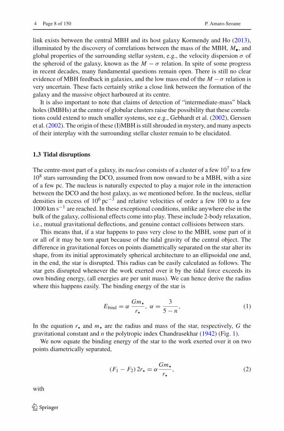
This means that, if a star happens to pass very close to the MBH, some part of itor all of it may be torn apart because of the tidal gravity of the central object. Thedifference in gravitational forces on points diametrically separated on the star alter itsshape, from its initial approximately spherical architecture to an ellipsoidal one and,in the end, the star is disrupted. This radius can be easily calculated as follows. Thestar gets disrupted whenever the work exerted over it by the tidal force exceeds itsown binding energy, (all energies are per unit mass). We can hence derive the radiuswhere this happens easily. The binding energy of the star is
Ebind = αGm�
r�, α = 3
5 − n, (1)
In the equation r� and m� are the radius and mass of the star, respectively, G thegravitational constant and n the polytropic index Chandrasekhar (1942) (Fig. 1).
We now equate the binding energy of the star to the work exerted over it on twopoints diametrically separated,
(F1 − F2) 2r� = αGm�
r�, (2)
with
123

Relativistic dynamics and extreme mass ratio inspirals Page 9 of 150 4
F2 F1
r�
M•
rt
Fig. 1 Decomposition of the tidal forces over a star. The tidal radius is rt , M• the mass of the MBH andF1, F2 the forces exerted on two points of the star which are diametrically separated
F1 = GM•(rt − r�)2 ,
F2 = GM•(rt + r�)2 . (3)
Considering r� � rt , we can approximate the expressions:
1
(rt − r�)2 ≈ 1
r2t
+ 2r�r3
t
1
(rt + r�)2 ≈ 1
r2t
− 2r�r3
t; (4)
then,
rt =[
2
3(5 − n)
M•m�
]1/3
r�. (5)
For solar-type stars it is (considering a n = 3 polytrope)
rt � 1.4 × 10¹¹(M•M�
)1/3
cm. (6)
In Fig. 2, I show the simulation of the tidal disruption of a star. The initial sphericalarchitecture of the star is altered after the passage through periapsis, as we can see inthe second snapshot. The third and fourth panels show the star at much later times. Wecan see the core of the star in the last one, idenfitied as a bright, spherical condensateof SPH particles.
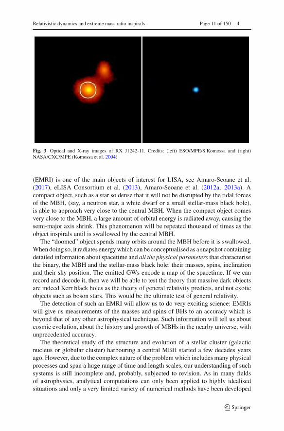
Figure 3 (left) shows a Chandra X-ray image of J1242-11 with a scale of 40 arcsecon a side. This figure pinpoints one of the most extreme variability events ever detectedin a galaxy. One plausible explanation for the extreme brightness of the ROSAT sourcecould be accretion of stars on to a super-massive black hole. On the right, we haveits optical companion piece, obtained with the 1.5 m Danish telescope at ESO/LaSilla. The right circle indicates the position of the Chandra source in the centre of thebrighter galaxy.
These processes may contribute significantly to the mass of the MBH, see e.g., Mur-phy et al. (1991), Freitag and Benz (2002). Tidal disruptions trigger phases of bright
123

4 Page 10 of 150 P. Amaro-Seoane
Fig. 2 Four snapshots in the evolution of a tidal disruption of a star. In this simulation, which I have donewith GADGET-2 (Springel 2005), the star is modelled as a polytrope using 5 ·104 particles. The penetrationfactor, which is defined to be the ratio between the tidal radius and the distance of periapsis, has been setto 9. The mass of the MBH is 106 M� and of the star 1 M�. The snapshots correspond to the initial time,and three later moments in the evolution. The left and right quick response codes link to two movies in theframe of the star and the general one, which point to the URLs https://youtu.be/Ryc44v4Eb7I and https://youtu.be/uZqXBD8R9Dw, respectively
accretion that may reveal the presence of a MBH in an otherwise quiescent, possiblyvery distant, galaxy (Hills 1975; Gezari et al. 2003).
1.4 Extreme mass ratio inspirals
On the other hand, stars can be swallowed whole if they are kicked directly throughthe horizon of the MBH (the so-called direct plunges) or gradually inspiral due tothe emission of GWs The latter process, known as an “extreme mass ratio inspiral”
123
Relativistic dynamics and extreme mass ratio inspirals Page 11 of 150 4
Fig. 3 Optical and X-ray images of RX J1242-11. Credits: (left) ESO/MPE/S.Komossa and (right)NASA/CXC/MPE (Komossa et al. 2004)
(EMRI) is one of the main objects of interest for LISA, see Amaro-Seoane et al.(2017), eLISA Consortium et al. (2013), Amaro-Seoane et al. (2012a, 2013a). Acompact object, such as a star so dense that it will not be disrupted by the tidal forcesof the MBH, (say, a neutron star, a white dwarf or a small stellar-mass black hole),is able to approach very close to the central MBH. When the compact object comesvery close to the MBH, a large amount of orbital energy is radiated away, causing thesemi-major axis shrink. This phenomenon will be repeated thousand of times as theobject inspirals until is swallowed by the central MBH.
The “doomed” object spends many orbits around the MBH before it is swallowed.When doing so, it radiates energy which can be conceptualised as a snapshot containingdetailed information about spacetime and all the physical parameters that characterisethe binary, the MBH and the stellar-mass black hole: their masses, spins, inclinationand their sky position. The emitted GWs encode a map of the spacetime. If we canrecord and decode it, then we will be able to test the theory that massive dark objectsare indeed Kerr black holes as the theory of general relativity predicts, and not exoticobjects such as boson stars. This would be the ultimate test of general relativity.
The detection of such an EMRI will allow us to do very exciting science: EMRIswill give us measurements of the masses and spins of BHs to an accuracy which isbeyond that of any other astrophysical technique. Such information will tell us aboutcosmic evolution, about the history and growth of MBHs in the nearby universe, withunprecedented accuracy.
The theoretical study of the structure and evolution of a stellar cluster (galacticnucleus or globular cluster) harbouring a central MBH started a few decades yearsago. However, due to the complex nature of the problem which includes many physicalprocesses and span a huge range of time and length scales, our understanding of suchsystems is still incomplete and, probably, subjected to revision. As in many fieldsof astrophysics, analytical computations can only been applied to highly idealisedsituations and only a very limited variety of numerical methods have been developed
123

4 Page 12 of 150 P. Amaro-Seoane
so far that can tackle this problem. In the next sections I will address the most relevantastrophysical phenomena for EMRIs and in the last section I give a description of afew different approaches to study these scenarios with numerical schemes.
2 GWs as a probe to stellar dynamics and the cosmic growth of SMBHs
2.1 GWs and stellar dynamics
The challenge of detection and characterisation of gravitational waves is stronglycoupled with the dynamics of dense stellar systems. This is especially true in the caseof the capture of a compact object by a MBH.
In order to estimate how many events one can expect and what we can assessabout the distribution of parameters of the system, we need to have a very detailedcomprehension of the physics. In this regard, the potential detection of GWs is anincentive to dive into a singular realm otherwise irrelevant for the global dynamics ofthe system.
As mentioned, a harbinger in this respect has been the tidal disruption of stars as away to feed the central MBH. About 50% of the star is bound to the MBH and accretedon to it, producing an electromagnetic flare which tops out in the UV/X-rays, emittinga luminosity close to Eddington. Nonetheless, the complications of accretion are par-ticularly intricate, tight on many different timescales to the microphysics of gaseousprocesses. Even on local, galactic accreting objects the complications of accretion areconvoluted. It is thus extremely difficult to understand how to extract very detailedinformation about extragalactic MBHs from the flare. The question of feeding a MBHis a statistical one. We do not care about individual events to understand the growthin mass of the hole, but about the statistics of the rates on cosmological timescales.Obviously, if we tried to understand the individual processes, we would fail.
As for the fate a compact object which approaches the central MBH, this was neveraddressed before we had the incentive of direct detection of gravitational radiation.Astrophysical objects such as a black hole binary, generate perturbations in spaceand time that spread like ripples on a pond. Such ripples, known as “gravitationalwaves” or “gravitational radiation”, travel at the speed of light, outward from theirsource. These gravitational waves are predicted by general relativity, first proposedby Einstein. Measurement of these gravitational waves give astrophysicists a totallynew and different way of studying the Universe: instead of analysing the propagationand transformation of particles such as photons, we have direct information from thefabric of spacetime itself. The information carried by the gravitational radiation willtell us in exquisite detail about the history, behaviour and structure of the universe:from the Big Bang to black holes.
When we started to look into this problem, we realised that there were many ques-tions of stellar dynamics that either did not have an answer or that had not even beenaddressed at all. In this review I will discuss the relaxation processes that we know toplay a major role in the dynamics of this particular regime. This involves two-bodyas well as many-body-coherent or non-coherent relaxation, and relativity. The list
123
Relativistic dynamics and extreme mass ratio inspirals Page 13 of 150 4
of processes is most likely incomplete, for there can still be additional, even morecomplicated processes unknown to us. We now have more questions than answers.
2.2 The mystery of the growth of MBHs
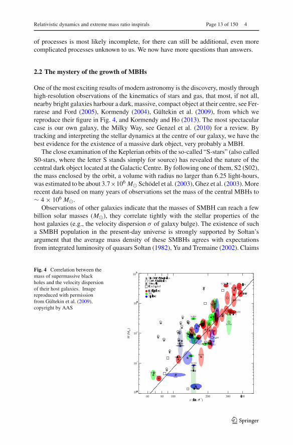
One of the most exciting results of modern astronomy is the discovery, mostly throughhigh-resolution observations of the kinematics of stars and gas, that most, if not all,nearby bright galaxies harbour a dark, massive, compact object at their centre, see Fer-rarese and Ford (2005), Kormendy (2004), Gültekin et al. (2009), from which wereproduce their figure in Fig. 4, and Kormendy and Ho (2013). The most spectacularcase is our own galaxy, the Milky Way, see Genzel et al. (2010) for a review. Bytracking and interpreting the stellar dynamics at the centre of our galaxy, we have thebest evidence for the existence of a massive dark object, very probably a MBH.
The close examination of the Keplerian orbits of the so-called “S-stars” (also calledS0-stars, where the letter S stands simply for source) has revealed the nature of thecentral dark object located at the Galactic Centre. By following one of them, S2 (S02),the mass enclosed by the orbit, a volume with radius no larger than 6.25 light-hours,was estimated to be about 3.7×10⁶ M� Schödel et al. (2003), Ghez et al. (2003). Morerecent data based on many years of observations set the mass of the central MBHs to∼ 4 × 10⁶ M�.
Observations of other galaxies indicate that the masses of SMBH can reach a fewbillion solar masses (M�), they correlate tightly with the stellar properties of thehost galaxies (e.g., the velocity dispersion σ of galaxy bulge). The existence of sucha SMBH population in the present-day universe is strongly supported by Sołtan’sargument that the average mass density of these SMBHs agrees with expectationsfrom integrated luminosity of quasars Sołtan (1982), Yu and Tremaine (2002). Claims
Fig. 4 Correlation between themass of supermassive blackholes and the velocity dispersionof their host galaxies. Imagereproduced with permissionfrom Gültekin et al. (2009),copyright by AAS
123
4 Page 14 of 150 P. Amaro-Seoane
of detection of “intermediate-mass” black holes (IMBHs, with masses ranging between100 − 104 M�) at the centre of globular clusters Gebhardt et al. (2002), Gerssen et al.(2002) raise the possibility that these correlations extend to much smaller systems, butso far the strongest, although not conclusive, observational support for the existenceof IMBHs are ultra-luminous X-ray sources Miller and Colbert (2004), Kong et al.(2010).
Although there is an emerging consensus regarding the growth of large-mass MBHsthanks to Sołtan’s argument, MBHs with masses up to 107 M�, such as our own MBHin the Galactic Centre (with a mass of ∼ 4 × 10⁶ M�), are enigmatic. There aremany different explains of their masses: accretion of multiple stars from arbitrarydirections, see Phinney (1989), Magorrian and Tremaine (1999), Syer and Ulmer(1999), Hills (1975), Rees (1988), mergers of compact objects such as stellar-massblack holes and neutron stars, see Quinlan and Shapiro (1990), or IMBHs falling onto the MBH, Portegies Zwart et al. (2006). Other more peculiar means are accretionof dark matter Ostriker (2000) or collapse of supermassive stars Hara (1978), Shapiroand Teukolsky (1979), Rees (1984), Begelman (2010). The origin of these low-massMBHs and, therefore, the early growth of all MBHs, remains a conundrum.
The centre-most part of a galaxy, its nucleus, consists of a nuclear star cluster ofa few millions of stars surrounding the MBH, see Schödel et al. (2014). The nucleusis naturally expected to play a major role in the interaction between the MBH andthe host galaxy. In the nucleus, stellar densities in excess of a million stars per cubicparsec and relative velocities of the order ∼ 100–1000 km s−1can be reached. In theseconditions, as mentioned before, collisional effects are important come into play. Thisis true except in globular clusters, but one important difference is that the SMBHgives the central part of the cluster almost a Keplerian potential, and thus very trickyresonance characteristics. This is one reason it has been difficult to analyse the starshere.
2.3 A magnifying glass
The laser interferometer space antenna (LISA), see in particular the document pre-pared in response to the call for missions for the L3 slot in the Cosmic VisionProgramme, Amaro-Seoane et al. (2017), but also Danzmann (2000), Amaro-Seoaneet al. (2012a, 2013a), will be our reference point throughout my review. LISA consistsof three spacecraft arranged in an equilateral triangle with sides of length 2.5 millionkilometre. LISA will scan the entire sky and covers a band from below 10−4 Hz toabove 10−1 Hz. In this frequency band, the Universe is populated by strong sources ofGWs such as binaries of supermassive black holes merging in the centre of galaxies,massive black holes “swallowing” entirely small compact objects like stellar-massblack holes, neutron stars and white dwarfs. The information is encoded in the grav-itational waves: the history of galaxies and black holes, the physics of dense matterand stellar remnants like stellar-mass black holes, as well as general relativity and thebehaviour of space and time itself. Chinese mission study options, such as Taiji, Ben-der et al. (2005a), Gong et al. (2011, 2015), Huang et al. (2017) will also be able tocatch these systems with good signal-to-noise ratios.
123

Relativistic dynamics and extreme mass ratio inspirals Page 15 of 150 4
Fig. 5 Amplitude spectral density of LISA Pathfinder as compared to the previous publication of the LPFgroup (Armano et al. 2016), which is the curve in blue. The data are compare with LISA requirements, aspresented in Amaro-Seoane et al. (2017). We can see that LISA Pathfinder exceeds the requirements forkey technologies for LISA over a factor of two over the entire observation band. Image reproduced withpermission from Armano et al. (2018), copyright by the authors
In any case, a key property of GW astrophysics is the fact that GWs interact onlyvery weakly with matter, except for high-z. The observations we will make with LISAwill not suffer any of the usual problems in astrophysics—absorption, scattering, orobscuration. This is what makes LISA-like missions such as LISA or Taiji unique. Itis not “merely” a test of general relativity; these missions would be able to corroboratethe underlying theory of the nature of the central dark objects which we now observein most galaxies. We will get direct information from the heart of the densest stellarsystems in the Universe: galactic nuclei, nuclear stellar clusters and globular clusters.The LISA mission technology has been successfully tested with the LISA Pathfinder5
mission, an ESA-led mission with a contribution from NASA, launched in 2015 fromKourou, French Guiana. Figure 5 is reproduced from Armano et al. (2018). Thispublication has remarkably improved the previous results of Armano et al. (2016),which showed that LISA Pathfinder has satisfied the mission requirements by factorsranging from 10 to 1000 depending on the frequency range, achieving a sub-Femto-gin free fall (Armano et al. 2016). Indeed, the results published in 2018 show that,actually, LISA Pathfinder has exceeded the requirements for LISA by more than afactor of two over the whole observation band (down to 20 μHz).
For the full success of a mission such as LISA, it is important that we understand thesystems that we expect to observe. A deep theoretical comprehension of the sourceswhich will populate LISA’s field of view is important to achieve its main goals.
Whilst main-sequence stars are tidally disrupted when approaching the centralMBH, compact objects (stellar-mass black holes, neutron stars, and white dwarfs)slowly spiral into the MBH and are swallowed whole after some ∼ 105 orbits in theLISA band. At the closest approach to the MBH, the system emits a burst of GWs
5 http://sci.esa.int/lisapf.
123
4 Page 16 of 150 P. Amaro-Seoane
which contains information about spacetime and the masses and spins of the system.We can envisage each such burst as a snapshot of the system. This is what makesEMRIs so appealing: a set of ∼ 105 bursts of GWs radiated by one system will tell uswith the utmost accuracy about the system itself, it will test general relativity, it willtell us about the distribution of dark objects in galactic nuclei and globular clusters and,thus, we will have a new understanding of the physics of the process. New phenomena,unknown and unanticipated, are likely to be discovered.
If the central MBH has a mass larger than 107 M�, then the signal of an inspiralingstellar-mass black hole, even in its last stable orbit (LSO) will have a frequency toolow for detection. On the other hand, if it is less massive than 104 M�, the signal willalso be quite weak unless the source is very close. This is why one usually assumesthat the mass range of MBHs of interest in the search of EMRIs for LISA is between[107, 104] M�. Nonetheless, if the MBH is rotating rapidly, then even if it has a masslarger than 107 M�, the LSO will be closer to the MBH and thus, even at a higherfrequency, the system should be detectable. This would push the total mass to a few∼ 107 M�.
For a binary of a MBH and a stellar-mass black hole to be in the LISA band, it hasto have a frequency of between roughly 10−5 and 1 Hz. The emission of GWs is moreefficient as they approach the LSO, so that LISA will detect the sources when they areclose to the LSO. The total mass required to observe systems with frequencies between0.1 Hz and 10−4 is of 104–107 M�. For masses larger than 107 M�, the frequenciesclose to the LSO will be too low, so that their detection will be very difficult. On theother hand, for a total mass of less than 103 M� we could in principal detect them atan early stage, but then the amplitude of the GW would be rather low.
On top of this, the measurement of the emitted GWs will give us very detailedinformation about the spin of the central MBH. With current techniques, we can onlyhope to measure MBH spin through X-ray observations of Fe Kα profiles, but thenumerous uncertainties of this technique may disguise the real value. Moreover, suchobservations can only rarely be made.
This means that LISA will scrutinise exactly the range of masses fundamental tothe understanding of the origin and growth of supermassive black holes. By extractingthe information encoded in the GWs of this scenario, we can determine the redshiftedmass and spin of the central MBH with an astonishing relative precision. Additionally,the mass of the compact object which falls into the MBH and the eccentricity of theorbit will be recovered from the gravitational radiation with a tiny fractional accuracy.All this means that LISA will not be “just” the ultimate test of general relativity, butan exquisite probe of the spins and range of masses of interest for theoretical andobservational astrophysics and cosmology.
2.3.1 A problem of ∼ 10 orders of magnitude
For the particular problem of how does a compact object end up being an extrememass ratio inspiral, we have to study very different astrophysical regimes, spanningover many orders of magnitude.
123
Relativistic dynamics and extreme mass ratio inspirals Page 17 of 150 4
Galactic or cosmological dynamics Figure 6 depicts the three different realms ofstellar dynamics of relevance for the problem of EMRIs. At the largest scale exists thegalaxy, with a size of a few kiloparsecs. Just as a point of reference, the gravitationalradius of a MBH of 106 M� ∼ 5 · 10−8 pc. The relaxation time, trlx which I willintroduce with more detail ahead, is a timescale which can be envisaged as the requiredtime for the stars to exchange energy and angular momentum between them: it is thetime that the stars need to “see” each other individually and not only the average,background stellar potential of the whole stellar system. For the galaxy, trlx is largerthan the Hubble time, which means that, on average, it has no influence on the galaxyat all. A test star will only feel the mean potential of the rest of the stars and it willnever exchange either energy or angular momentum with any other star. The system is“collisionless”, meaning that two-body interactions can be neglected. This defines therealm of stellar galactic dynamics, the one investigated in Cosmological simulationsusing, e.g., N -body integrators. Since we do not have to take into account the stronginteractions between stars, one can easily simulate ten billion particles with theseintegrators.
Cluster dynamics If we zoom in by typically a factor of 103, we enter the (mostlyNewtonian) stellar dynamics of galactic nuclei. There, trlx ∼ 108−1010 yrs. In thisrealm stars do feel the graininess of the stellar potential. The closer we get to thecentral MBH, the higher σ will be, if the system is in centrifugal equilibrium; thestars have to orbit around the MBH faster. In particular, S2 (or S02), one of the S-stars(S0-stars) for which we have enough data to reconstruct the orbit to a very high levelof confidence—as we saw in the previous section—has been observed to move with avelocity of 15 · 103 km s−1. Typically, trlx is (on occasion much) shorter than the ageof the system, of a few ∼ 108 − 1010 yrs. For these kind of systems one has to takeinto account relaxation, exchange of energy and angular momentum between stars.The system is “collisional”. When we have to take into account this in the numericalsimulations, the result is that we cannot simulate with N -body integrators more thansome thousands of stars on a regular computer. To get to more realistic particle numbersone has to resort to many computers operating in parallel, special-purpose hardwareor the graphic processor units. I will discuss this later.
Relativistic stellar dynamics Last, in the right panel of Fig. 6, we have the relativisticregime of stellar dynamics when we enlarge the previous by a factor of ten million.There the role of relativistic effects is of paramount importance for the evolution ofthe system. In this zone, generally, there are no stars. Even at the densities whichcharacterise a galactic nucleus, the probability of having a star in such a tiny volumeis extremely small. Moreover, even if we had a significantly larger volume, or a muchhigher density for the galactic nucleus, so that we had a few stars close to the MBH,these would quickly merge with the MBH due to the emission of GWs, which iswhat defines an EMRI. But they do it too fast. These systems can be collisionalor collisionless, depending on how many stars we have at a given time. If they arethere, they will exchange energy and angular momentum between them. Nevertheless,relaxation is not well-defined in this regime.
123

4 Page 18 of 150 P. Amaro-Seoane
RSchw = 10−7 − 10−4 pc
ρ�, gal ∼ 0.05M�pc−3
σ�, gal ∼ 40 km s−1
trlx, gal ∼ 1015 yrs
M• ∼ 106 − 109M�
ρ�, cl ∼ 106 − 108M� pc−3
σ�, cl ∼ 100 − 1000 km s−1
trlx, cl ∼ 108 − 1010 yrs
Fig. 6 On the left, and with the largest scale, the galaxy has an average density of stars of about0.05 M�pc−3. The velocity dispersion is ∼ 40 km s−1. From these quantities one can infer that the relax-ation time in the vicinity of our Sun is trlx ∼ 1015 yrs. The upper panel shows the galactic nucleus thatsuch a galaxy has. A typical size for it is ∼ 1 pc, the stellar density ranges between 106 − 108 M� pc−3
and the velocity dispersion is of σ ∼ 100 − 1000 km s−1. In this region, trlx ∼ 108 − 1010 yrs. In the lastpanel, we have that the dynamics of the system is dominated by General Relativity. As a reference point,the Schwarzschild radius of a 106 M� (109 M�) is 10−7 pc (10−4 pc)
The key point here is how to replenish that area, so that there are other stars replacingthose which merge quickly with the central MBH. On average, there are zero stars.As a matter of fact, and in general, for the general study of the stellar dynamics ofgalactic nuclei, the role of this last realm is negligible. One does not have to botherwith the effects of GR; most, if not all, stars are on a Newtonian regime. The impact onthe dynamics of galactic nuclei is zero. It is impressive that this last region dominatedby the effects of GR has an effect worth studying at all. But, as we will see ahead,the encoded information that one can recover from the detection of an EMRI aboutits surrounding dynamical system is dramatic. If we want to address this problem, weneed to cope with a range of scales that spans over seven orders of magnitude whenunderstanding the role of the dynamics of galactic nuclei in relativistic dynamics, andof ten orders of magnitude in the big picture.
2.4 How stars distribute around MBHs in galactic nuclei
In Fig. 7 I show data constrained by electromagnetic measurements. One of the veryfirst questions one has to address when trying to understand the stellar dynamics arounda MBH is howmany stars are there and howdo they distribute around it? Unfortunatelythere are very few observations for this because we are interested in nuclei that harbourlower-mass MBHs, i.e., with masses ranging 104 and 106 M�, so that they thereforehave a small radius of influence rinf and, thus, they are observationally very difficultto resolve. Currently there are only a very few galaxies that are both in the range ofGW frequencies interesting to us and that have a resolved rinf . For these we have
123

Relativistic dynamics and extreme mass ratio inspirals Page 19 of 150 4
Fig. 7 Density profile for theGC of the MW and for M32,both with MBHs of masses3 × 106 M� and influence radii∼ 3 pc. The dashed curve on thevery left corresponds to a slopeof ρ ∝ r−3/2. Image adaptedfrom Merritt (2006), Schödelet al. (2002), Lauer et al. (1998)
ρ ∝ r−1.5
information on how bound stars that can become EMRIs are distributed around thecentral MBH. Obviously, the Milky Way (MW) is one of these galaxies. In Fig. 7the stellar density profile of the MW is displayed. We see that it goes up to at least108 M�/pc3 in the inner regions. This number has been calculated by assuming apopulation of stars; one has to deproject the observation, because we are only seeinga few of the total amount of stars, the brightest ones. One assumes that the observedstars are tracing an underlying population invisible to us. This requires a considerableamount of modelling to obtain the final results. These are uncertain by, at most, a factorof ten. In the same figure we have another nucleus, M32, which should be harbouringa MBH with a mass similar to the one located in the GC. The density profile happensto be similar to the one corresponding to the GC. Whether this is a coincidence orsomething deeper is not clear. In any case, and to first order of approximation, wecan state that once we know the mass of the MBH, we know the way stars distributearound it. Later the relevance of this point will be obvious to the reader.
3 A taxonomy of orbits in galactic nuclei
Before we address the physics and event rate estimates of EMRIs, it is crucial thatwe have a good understanding of the kind of orbits that we might expect in the envi-ronments natural to COs in dense systems around a MBH. An important factor inunderstanding how a star can become an EMRI is the shape and evolution of its orbit.In this section, I will address these two aspects. First, we will not take into accountthe role of relaxation. The stellar potential in which our test star m• is moving iscompletely smooth. For any purpose, the test star will not feel any individual star, buta background potential.
123

4 Page 20 of 150 P. Amaro-Seoane
m•
Rinfl
M•
m•
M•
Rinfl
Fig. 8 Projection in the X–Y plane of the evolution of two test star orbits in a stellar system withoutrelaxation. The central, orange point represents the position of the MBH, the black dots on the orbits theposition of the test stars and the red arrow delimits the influence radius Rinfl of the MBH. The right panelrepresents a case with a larger eccentricity. The orbits extend further than the Rinfl
3.1 Spherical potentials
Consider now Fig. 8; there we have two orbits which differ in their eccentricity. Therosettes are characterised by their energy and angular momentum. Since the test starsdo not suffer any individual gravitational tug from the stellar system (at least not ona noticeable timescale), the orbital elements are kept constant. The periapsis6 is fixedbecause the angular momentum is conserved, so that the test star will never comearbitrarily close to the central MBH. In order to achieve anything interesting, oneneeds to perturbate the system.
A different situation, however, is when the orbit of the test star is within the Rinfl ofthe MBH. In this case, the orbits look more and more like Keplerian ellipses, unless onegets very close to the central MBH, so that we get relativistic precession. In Fig. 9 wehave an ellipse which precesses with time. This is neither the relativistic precession noran advance, but a purely Newtonian perihelion (periapsis) retard, counterclockwise.The timescale for it is
TNew, PS ≈ M•M�(a)
Porb ≈ Rinfl
aPorb (7)
In this last equation, M�(a) is the amount of stellar mass encompassed within the orbit.The Newtonian periapsis retard is the result of the fact that we do not have a perfectKeplerian orbit because we do not have a point mass, but an extended mass distribution.As an exercise, we can compare the last equation to the relativistic periapsis advance(in order of magnitude),
6 In the related literature there exist other terms to refer to the distance of maximum or minimum approachto a black hole; namely peribarathron and apobarathron, respectively. There seems to be a confusion andwrong use of the later. I discuss this in Sect. A.
123

Relativistic dynamics and extreme mass ratio inspirals Page 21 of 150 4
Rapo = 0.4Rinfl
M•
m• m•M•
Rinfl
Rapo = 0.8Rinfl
Fig. 9 Same as Fig. 8 for an apoapsis Rapo = 0.4, 0.8 Rinfl and a velocity of the CO of 0.2 Vcirc, withVcirc the circular velocity
TRel, PS ≈ Rperi
RSchwPorb (8)
This equation is only relevant for orbits whose periapsis is very small, whilst the laterone is only important for relatively extended orbits (because M�(a) is larger)
3.2 Non-spherical potentials
The most general case is the triaxial potential, in which we still have symmetry butneither spherical nor axial-symmetry, it is a general ellipsoidal configuration. Theangular momentum has no component conserved. This, obviously, allows orbits toget “as close as they want” to the centre. Not all orbits will, but there are specificfamilies of orbits which, if one waits long enough, will get arbitrarily close to thecentre. This is evidently very relevant for our study. These orbits are refered to ascentrophilic orbits for clear reasons. Studies of models of triaxial galaxies have foundthat there is a significant fraction of such orbits even very close to the central MBH.At distances as short as r < Rinfl, within the sphere of influence, some models have asmany as 20% of stars that are on centrophilic orbits. One should nevertheless bear inmind that these are models, not corroborated by direct observations of galaxies. Theydepend on a number of set-up parameters which will result in strong fluctuations of thefinal result: the true number could be between 0 and 20% according to these models.Therefore, unfortunately we do not know what the real implications are for observednuclei, since it is not well-constrained. Of course, one can resort to (non-collisional)N -body simulations to study the merger of two galaxies to see in the resulting producthow many of these orbits one can get (Figs. 10, 11).
As for the implications of the detection rates of EMRIs, this could have a hugeimpact, but the problem should probably be revisited due to the enormous difficul-ties that force us to make broad simplifications. For instance, we should explore thebehaviour of the potential very close to the MBH because, by definition, at some point
123

4 Page 22 of 150 P. Amaro-Seoane
M•
Rapo = 0.1Rinfl
m•
v = 0.2Vcirc
m•
Rapo = 0.1Rinfl
M•
v = 0.5Vcirc
Fig. 10 Same as Figs. 8 and 9 for different values of the apoapsis radius and velocity of the CO
Fig. 11 In the Newtonian case we have an extended mass distribution, so that the star feels more mass faraway than closer to the centre. When the star traverses the “sphere”, the trajectory abruptly changes andbecomes a smaller ellipse Thus, the object goes back to the centre faster; the orbit precesses in the oppositedirection to the orbital one In the relativistic case the kinetic energy of the star increases its gravitationalmass when it’s close to the centre: The effective attraction is more efficient and the trajectory is more curvedtowards the centre
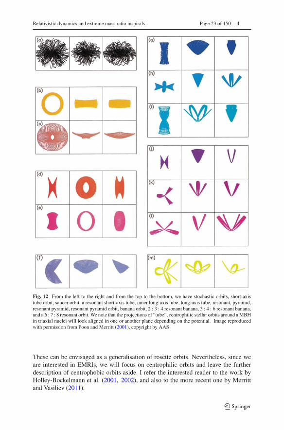
the potential is completely dominated by the MBH and, thus, spherically symmetric.The only realistic hope here are those stars that typically are on orbits with semi-majoraxis much larger than the radii of interest to us, so that even if they spend most of thetime very far away from the MBH, they will be set on a centrophilic orbit due to thetriaxiality of the system, but it is unclear whether these can contribute significantlyto the local density around the MBH. As an example of the kind of orbits one canget in a triaxial galactic nucleus, in Fig. 12 I show some representative examples ofcentrophobic orbits from Poon and Merritt (2001) (cases b, c, d, e). This means thatthe stars never reach the centre. The lack of conservation of the angular momentumcan set stars on either centrophilic orbits or, alternatively, on centrophobic orbits.
123
Relativistic dynamics and extreme mass ratio inspirals Page 23 of 150 4
Fig. 12 From the left to the right and from the top to the bottom, we have stochastic orbits, short-axistube orbit, saucer orbit, a resonant short-axis tube, inner long-axis tube, long-axis tube, resonant, pyramid,resonant pyramid, resonant pyramid orbit, banana orbit, 2 : 3 : 4 resonant banana, 3 : 4 : 6 resonant banana,and a 6 : 7 : 8 resonant orbit. We note that the projections of “tube”, centrophilic stellar orbits around a MBHin triaxial nuclei will look aligned in one or another plane depending on the potential. Image reproducedwith permission from Poon and Merritt (2001), copyright by AAS
These can be envisaged as a generalisation of rosette orbits. Nevertheless, since weare interested in EMRIs, we will focus on centrophilic orbits and leave the furtherdescription of centrophobic orbits aside. I refer the interested reader to the work byHolley-Bockelmann et al. (2001, 2002), and also to the more recent one by Merrittand Vasiliev (2011).
123

4 Page 24 of 150 P. Amaro-Seoane
We have two different kinds of centrophilic orbits: (i) pyramid or box orbits. Theseare still regular but a star on such an orbit can reach arbitrarily small distances in itsperiapsis; (ii) stochastic orbits, which also come arbitrarily close to the centre. Theprobability for an orbit to get within a distance d from the central MBH, the verycentre of the potential, is proportional to d.
This is non-intuitive. If you have a target with a mass and you shoot a projectilefrom random directions, the probability of coming within a distance d of the targetRp < d is proportional to d itself and not d2 (which would have been the case for atotally random experiment, without focusing). In the case of a star on an orbit towardsthe MBH, the number of times you have to “throw” it to get to a periapsis distancecloser than d is, Npass (Rp < d) ∝ d. The reason for this is that our target is a particularone and influences the projectile through a process called gravitational focusing. Theprojectile, the star, is attracted by the target, the MBH.
Something to also bear in mind is that all of these simulations are limited by aparticular resolution, which is still far from being close to reality, so that we are notin the position of extrapolating these results to the distances where the star will becaptured by the MBH and become and EMRI.
4 Two-body relaxation in galactic nuclei
4.1 Introduction
We are now back to a spherical system world, in which orbits such as those in theprevious section do not exist. Therefore, one needs an additional factor to bring starsclose to the MBH. As I have already discussed before, a possibility, is to have asource of exchange of energy and angular momentum. We use and abuse the termcollisional to refer to any effect not present in a smooth, static potential, includingsecular effects. Among these, standard two-body relaxation excells not due to itsrelevance of contributing to EMRI sources, but due to the fact that this is the best-studied effect; namely the exchange of energy and angular momentum between starsdue to gravitational interactions.
Another possibility is physical collisions.7 The stars come so close to each otherthat they collide, they have a hydrodynamic interaction; the outcome depends on anumber of factors, but the stars involved in the collision could either merge with eachother or destroy each other completely or partially. Contrary to what one could expect,the impact of these processes for the global evolution of the dynamics of galactic nucleiis negligible Freitag and Benz (2002). In most of the cases, when these extended stars,such as main-sequence stars (MS) collide, they do not merge due to the very highvelocity dispersion, and they will also not be totally destroyed, because for that theywould need a nearly head-on collision, so that they have a partial mass-loss and are
7 The terminology is somehow, and as forewarned, misleading; whilst in general we refer to “collisional”to any effect leading to exchange of energy and angular momentum among stars, here I mean real collisionsbetween two stars. For a thorough discussion of the mechanism and an extremely detailed numerical study,I refer the reader to Freitag and Benz (2002).
123

Relativistic dynamics and extreme mass ratio inspirals Page 25 of 150 4
for our purposes uninteresting. For the kind of objects of interest to us in this review,stellar-mass black holes, the probability that they physically collide is negligible.
A third way of altering the angular momentum of stars are secular effects. They donevertheless not modify the energy. If we assume that the orbits around the MBH arenearly Keplerian, the shape, an ellipse, does not change, and the orientation will notchange much. If we have another orbit with a different orientation, both orbits willexert a torque T on each other. This will change angular momentum but not energy.A Keplerian orbit can be described in terms of its semi-major axis and eccentricity.The semi-major axis is only connected to energy and, for a given semi-major axisthe eccentricity is connected to the angular momentum. If one changes the angularmomentum but not the energy, the eccentricity will vary but not the semi-major axis.By decreasing the angular momentum, one increases the eccentricity.
In this section, however, I introduce the fundamentals of relaxation theory, focusingon the aspects that will be more relevant for the main interest of this review. Furtherahead, in Sect. 7, I will address resonant relaxation and other “exotic” (in the sensethat they are not part of the traditional two-body relaxation theory) processes. Fora comprehensive discussion on two-body relaxation, I recommend the textbooks bySpitzer Jr (1969) and Binney and Tremaine (2008) or, for a shorter but very niceintroduction, the article by Freitag and Benz (2001).
I will first introduce handy timescales in Sect. 4.2 that will allow us to pinpointthe relevant physical phenomena that reign the process of bringing stars (extended orcompact) close to the central MBH. I will then address a particular case of relaxation, inSect. 4.3, dynamical friction. Later, in Sect. 4.4, I will define more concisely the regionof space-phase in which we expect stars to interact with the central MBH. Once we haveall these concepts, we can cope with the problem of how mass segregates in galacticnuclei, in Sect. 5. We will first see in detail the “classical” although academic solution,and later a more recent and physical result, the so-called strong mass segregation, inSect. 7.3
4.2 Two-body relaxation
I introduce now some useful time-scales to which I will refer often throughout thisreview; namely the relaxation time, the crossing time and the dynamical time. Thesethree time-scales allow us to delimit our physical system.
The relaxation time In Chandrasekhar (1942) a time-scale was defined which stemsfrom the 2-body small-angle encounters and gives us a typical time for the evolutionof a stellar system.
This relaxation time could be regarded as an analogy of the shock time of the gasdynamics theory, by telling us when a particle (a star) has forgotten its initial conditionsor, expressed in a different way, when the local thermodynamical equilibrium has beenreached. Then, we can roughly say that the most general idea is that this is the time overwhich the star “forgets” its initial orbit due to the series of gravitational tugs caused bythe passing-by stars. After a relaxation time the system has lost all information aboutthe initial orbits of all the stars. This means that the encounters alter the star orbit from
123
4 Page 26 of 150 P. Amaro-Seoane
θb
m2
m1
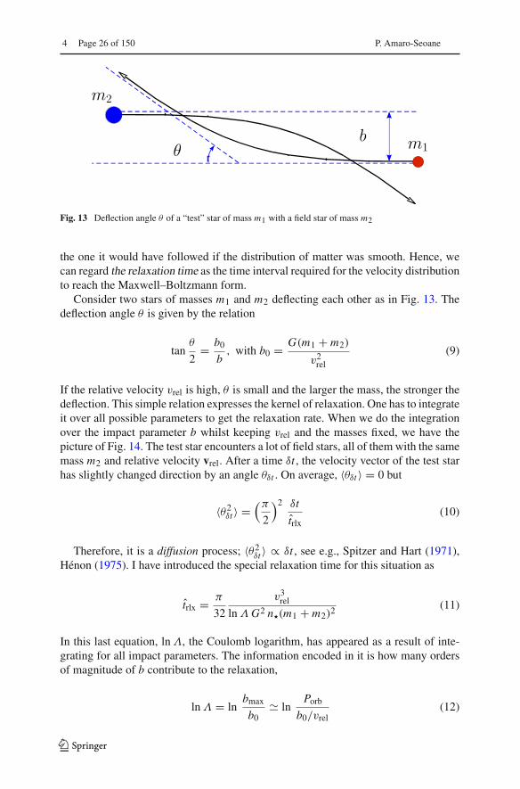
Fig. 13 Deflection angle θ of a “test” star of mass m1 with a field star of mass m2
the one it would have followed if the distribution of matter was smooth. Hence, wecan regard the relaxation time as the time interval required for the velocity distributionto reach the Maxwell–Boltzmann form.
Consider two stars of masses m1 and m2 deflecting each other as in Fig. 13. Thedeflection angle θ is given by the relation
tanθ
2= b0
b, with b0 = G(m1 + m2)
v2rel
(9)
If the relative velocity vrel is high, θ is small and the larger the mass, the stronger thedeflection. This simple relation expresses the kernel of relaxation. One has to integrateit over all possible parameters to get the relaxation rate. When we do the integrationover the impact parameter b whilst keeping vrel and the masses fixed, we have thepicture of Fig. 14. The test star encounters a lot of field stars, all of them with the samemass m2 and relative velocity vrel. After a time δt , the velocity vector of the test starhas slightly changed direction by an angle θδt . On average, 〈θδt 〉 = 0 but
〈θ2δt 〉 =
(π
2
)2 δt
trlx(10)
Therefore, it is a diffusion process; 〈θ2δt 〉 ∝ δt , see e.g., Spitzer and Hart (1971),
Hénon (1975). I have introduced the special relaxation time for this situation as
trlx = π
32
v3rel
ln ΛG2 n�(m1 + m2)2 (11)
In this last equation, ln Λ, the Coulomb logarithm, has appeared as a result of inte-grating for all impact parameters. The information encoded in it is how many ordersof magnitude of b contribute to the relaxation,
ln Λ = lnbmax
b0� ln
Porb
b0/vrel(12)
123

Relativistic dynamics and extreme mass ratio inspirals Page 27 of 150 4
m1
δtm2
vrel
n�
θδt
Fig. 14 The test stars suffers a change in direction by θδt due to the accumulation of encounters with fieldstars
In this last equation b0, which I introduced before, is the effective minimum impactparameter for relaxation. Our main focus is not a detailed review of stellar dynamics.For a detailed description of the Coulomb logarithm, I refer the reader to Binney andTremaine (2008), Spitzer Jr (1987). Therefore, I will simply comment that, for ourpurposes, ln Λ ≈ 10−15 always. This is very useful because the exact calculationcan be rather arduous and almost an incubus which to our knowledge nobody hasattempted to implement in any calculation. Therefore we mention only two specialcases for the argument of the logarithm,
Λ ≈⎧⎨⎩
0.01 N� (a) for a self-gravitatingstellar cluster
M•/m (b) close to the MBH(13)
In case (a), we have a self-gravitating cluster of stars in equilibrium with itself butlacking a central MBH. The argument is proportional to the number of stars in thesystem. In the situation in which a star is orbiting the MBH, the previous value isformally no longer valid and one should use the value (b). Nevertheless, in effect thisis neglected because the value turns out to be ∼ 10. To define a local average value ofthe relaxation time we integrate over the distribution of relative velocities.
It must, nevertheless, be noted that the way in which I have introduced the conceptof the relaxation time is a particular one. In Eq. (11), I have introduced the “encounterrelaxation time” to stress that it depends on the characteristics of a peculiar class ofencounter: a star of mass m1 with “field stars” of mass m2 with a local density n� anda relative velocity vrel. It can be envisaged as the required time to deflect graduallythe motion of star m1 due to encounters with field stars by a root mean square (RMS)angle π/2. This definition is useful to understand the fundamentals of relaxation, butit must be noted that it is subject to this very peculiar type of encounter.
However, in a general case, we define relaxation by simplifying the problem: (i)We restrict to the radius of influence for a system in which the distribution of stars isspherically symmetric, (ii) stars are treated as single objects, with a two-body relax-
123

4 Page 28 of 150 P. Amaro-Seoane
ation as the only mechanism that can change the angular momentum, and (iii) weneglect mass segregation.
The influence radius within which the central MBH dominates the gravitationalfield is
rinfl = GM•σ 2
0
≈ 1 pc
(M•
106 M�
)(60 km/s
σ0
)2
. (14)
Hence, in our approximation, the relaxation time is
trlx(r) = 0.339
ln Λ
σ 3(r)
G2〈m〉mCOn(r)
� 1.8 × 10⁸ yr
(σ
100 km s−1
)3 (10 M�mCO
)(106 M�pc−3
〈m〉n)
. (15)
Here, σ(r) is the local velocity dispersion. It is approximately equal to the Keplerianorbital speed
√GM•r−1 for r < rinfl and has a value ≈ σ0 outside of it. In the
expression n(r) is the local number density of stars, 〈m〉 is the average stellar mass,mCO is the mass of the compact object (we take a standard mCO = 10 M� for stellar-mass black holes).
For typical density profiles, trlx decreases slowly with decreasing r inside rinfl.It should be noted that the exchange of energy between stars of different masses—sometimes referred to as dynamical friction, as we will see ahead, in Sect. 4.3 in thecase of one or a few massive bodies in a field of much lighter objects—occurs on atimescale shorter than trlx by a factor of roughly M/〈m〉, where M is the mass of aheavy body.
As we will see later, relaxation redistributes orbital energy amongst stellar-massobjects until the most massive of them (presumably stellar-mass black holes) form apower-law density cusp around the MBH, n(r) ∝ r−γ with γ ranging between � 1.75–2.1, which depends on the solution to mass segregation considered, while less massivespecies arrange themselves into a shallower profile, with α � 1.4−1.5 (Bahcall andWolf 1976; Lightman and Shapiro 1977; Duncan and Shapiro 1983; Freitag and Benz2002; Amaro-Seoane et al. 2004; Baumgardt et al. 2004a; Preto et al. 2004; Freitag et al.2006b; Hopman and Alexander 2006a; Alexander and Hopman 2009; Merritt 2010;Preto and Amaro-Seoane 2010; Amaro-Seoane and Preto 2011; see also Sect. 8.7).Nuclei likely to host MBHs in the LISA mass range (M• � few × 106 M�) probablyhave relaxation times comparable to or less than a Hubble time, so that it is expectedthat their heavier stars form a steep cusp.
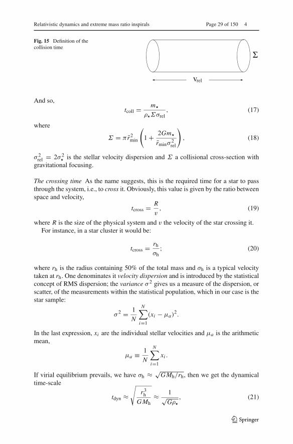
Collision time tcoll is defined as the required mean time for the number of stars withina volume V = Σvrel�t to be one (see Fig. 15), where vrel is the relative velocity atinfinity of two colliding stars.
Computed for an average distance of closest approach rmin = 23r�, this time is given
byn�V (tcoll) = 1 = n� Σ vrel tcoll. (16)
123
Relativistic dynamics and extreme mass ratio inspirals Page 29 of 150 4
Fig. 15 Definition of thecollision time
relv
Σ
And so,
tcoll = m�
ρ�Σσrel, (17)
where
Σ = π r2min
(1 + 2Gm�
rminσ2rel
), (18)
σ 2rel = 2σ 2
� is the stellar velocity dispersion and Σ a collisional cross-section withgravitational focusing.
The crossing time As the name suggests, this is the required time for a star to passthrough the system, i.e., to cross it. Obviously, this value is given by the ratio betweenspace and velocity,
tcross = R
v, (19)
where R is the size of the physical system and v the velocity of the star crossing it.For instance, in a star cluster it would be:
tcross = rh
σh; (20)
where rh is the radius containing 50% of the total mass and σh is a typical velocitytaken at rh. One denominates it velocity dispersion and is introduced by the statisticalconcept of RMS dispersion; the variance σ 2 gives us a measure of the dispersion, orscatter, of the measurements within the statistical population, which in our case is thestar sample:
σ 2 = 1
N
N∑i=1
(xi − μa)2.
In the last expression, xi are the individual stellar velocities and μa is the arithmeticmean,
μa ≡ 1
N
N∑i=1
xi .
If virial equilibrium prevails, we have σh ≈ √GMh/rh, then we get the dynamical
time-scale
tdyn ≈√
r3h
GMh≈ 1√
Gρ�
, (21)
123
4 Page 30 of 150 P. Amaro-Seoane
where ρ� is the mean stellar density.Contrary to gas dynamics, the thermodynamical equilibrium time-scale trlx in a
stellar system is large compared with the crossing time tcross. In a homogeneous,infinite stellar system, we expect some kind of stationary state to be established inthe limit t → ∞. The decisive feature for such a virial equilibrium is how quickly aperturbation of the system will be smoothed down.
The dynamical time in virial equilibrium is (cf., e.g., Spitzer Jr 1987):
tdyn ∝ log(γ N )
Ntrlx � trlx. (22)
If we have perturbations in the system because of the heat conduction, star accretionon to the MBH, etc. a new virial equilibrium will be established within a time tdyn,which is short. This means that we get again a virial-type equilibrium in a short time.This situation can be considered not far from a virial-type equilibrium. We say thatthe system changes in a quasi-stationary way.
4.3 Dynamical friction
Consider now a star more massive than the average. In this case, relaxation boils downto dynamical friction (DF). The massive intruder will suffer from dynamical friction,which is an effect of all encounters with lighter stars. For this special kind of star, thetimescale over which its orbital parameters change is not the relaxation time. This starwill lose kinetic energy in the following timescale:
tDF ∼ 〈m〉m
trlx. (23)
As we can see, if the object is 10–20 times more massive than the average, as in thecase of a stellar-mass black hole, this timescale is correspondigly 10–20 times shorterthan the trlx.
In Fig. 16 we have an illustration for what DF is. A massive intruder, a stellar-mass black hole, is travelling in a homogeneous sea of stars of density ρ and velocitydispersion σ . The velocity vectors of the stars is rotated after the deflection and theprojected component in the direction of the deflection is shorter. Therefore, the massiveobject is accumulating just after it a high-density stellar region. The perturber will feela drag from that region from the conservation of angular momentum in the directionof its velocity vector, just as depicted in Fig. 17. The direction does not change tofirst-order, but the amplitude decreases. The intruder will feel a force (acceleration)given by the Chandrasekhar formula,
aDF = − vtDF
− 4π ln ΛG2ρ M
v3 ξ(X)v. (24)
123

Relativistic dynamics and extreme mass ratio inspirals Page 31 of 150 4
M•ρ
σ
v
Fig. 16 In the reference frame of the encounter I depict a massive interloper, a stellar-mass black hole,traversing a sea of lighter stars which are deflected by it. The velocity vector of the stellar-mass black holeis bearely modified (at least in direction) by the deflections, because they cancel out on average
Fig. 17 The accumulation of stars right behind the massive perturber creates a region of stellar overdensitythat acts on the perturber, slowing it down, braking it
In this last equation,
ξ(X) = erf(X) − 2π−1/2Xe−X2,
X = v√2σ
(25)
123
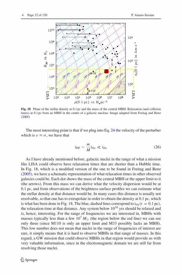
4 Page 32 of 150 P. Amaro-Seoane
LISA
LISA
Fig. 18 Plane of the stellar density at 0.1 pc and the mass of the central MBH. Relaxation (and collisiontimes) at 0.1 pc from an MBH in the centre of a galactic nucleus. Image adapted from Freitag and Benz(2005)
The most interesting point is that if we plug into Eq. 24 the velocity of the perturberwhich is v ≈ σ , we have that
tDF ∼ m
Mtrlx � trlx (26)
As I have already mentioned before, galactic nuclei in the range of what a missionlike LISA could observe have relaxation times that are shorter than a Hubble time.In Fig. 18, which is a modified version of the one to be found in Freitag and Benz(2005), we have a schematic representation of what relaxation times in other observedgalaxies could be. Each dot shows the mass of the central MBH or the upper limit to it(the arrows). From this mass we can derive what the velocity dispersion would be at0.1 pc, and from observations of the brightness surface profiles we can estimate whatthe stellar density at that distance would be. In many cases this distance is usually notresolvable, so that one has to extrapolate in order to obtain the density at 0.1 pc, whichis what has been done in Fig. 18. The blue, dashed lines correspond to trlx(r = 0.1 pc),the relaxation time at that distance. Any system below 1010 yrs should be relaxed andis, hence, interesting. For the range of frequencies we are interested in, MBHs withmasses typically less than a few 107 M� (the region below the red line) we can seeonly three (since M110 is only an upper limit and M33 possibly lacks an MBH).This low number does not mean that nuclei in the range of frequencies of interest arerare, it simply means that it is hard to observe MBHs in that range of masses. In thisregard, a GW mission that could observe MBHs in that region would provide us withvery valuable information, since in the electromagnetic domain we are still far fromresolving those nuclei.
123

Relativistic dynamics and extreme mass ratio inspirals Page 33 of 150 4
4.4 The difussion and loss-cone angles
As we have seen, the relaxation time is the required time to induce a change in theperpendicular velocity component of the same order as the perpendicular velocitycomponent itself, i.e., �v2⊥/v2⊥ � 1. Therefore,
�v2⊥ = nrlx · δv2⊥. (27)
Hence,
�v2⊥/v2⊥ = 1 = nrlx · δv2⊥v2⊥
. (28)
And then,
trlx = nrlx · tdyn =(
v2⊥δv2⊥
)· tdyn, (29)
wherenrlx is the numbers of crossings for �v2⊥/v2⊥ � 1. This conforms to the definitionof the relaxation time, �v2⊥/v2⊥ = t/trlx, see Binney and Tremaine (1987).
A useful quantity to derive is the diffusion angle, θD, which is defined to be themean deviation of a star orbit in a dynamical time, i.e., trlx � tdyn/θ
2D. I assume that
this angle must be a very small one, so that
sin θD � δv⊥v
� θD. (30)
Therefore,
θD �√tdyn
trlx. (31)
I now introduce the loss-cone angle θlc as an illustrative example. Suppose that thecentral object with mass M• has an influence radius rh. To define this radius we saythat a star will interact with the central object only when r ≤ rh. Then, we look for acondition at a place r > rh for a star to touch or to cross the influence radius of thecentral object within a crossing time tcross = r/σr.
I depict this in Fig. 19: A star on a certain orbit will get into the tidal disruptionradius of the MBH if its velocity vector is such that the distance of periapsis is withinthat radius. The velocity and radial distance vectors define the angle of the cone inphase-space for this to happen. Extended stars are torn apart and lost for the system,which is why we refer to that angle as the loss-cone angle. If the star is a stellar-massblack hole, it can withstand the tidal forces. Although I have also illustrated the effectof periapsis shift in the figure, I do not take it into account for the derivation of theloss-cone. It is meant to illustrate the complexity of the problem we are interested in,the gravitational capture of compact objects. As we have seen before, the conditionthat defines this angle is the following:
rp(E, L) ≤ rt,
θ ≤ θlc, (32)
123
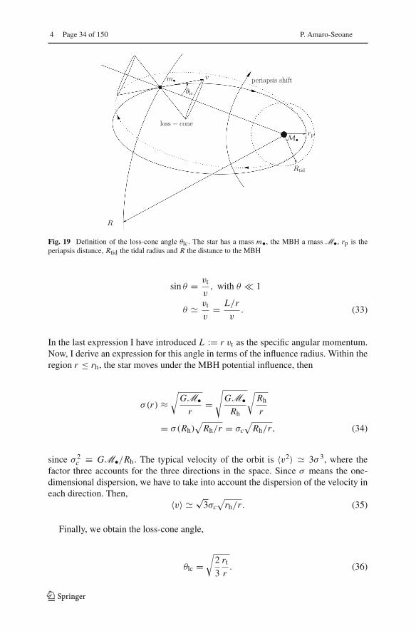
4 Page 34 of 150 P. Amaro-Seoane
θlc
R
rp
periapsis shift
Rtid
M•
loss − cone
vm•
Fig. 19 Definition of the loss-cone angle θlc. The star has a mass m•, the MBH a mass M•, rp is theperiapsis distance, Rtid the tidal radius and R the distance to the MBH
sin θ = vt
v, with θ � 1
θ � vt
v= L/r
v. (33)
In the last expression I have introduced L := r vt as the specific angular momentum.Now, I derive an expression for this angle in terms of the influence radius. Within theregion r ≤ rh, the star moves under the MBH potential influence, then
σ(r) ≈√GM•r
=√GM•Rh
√Rh
r
= σ(Rh)√Rh/r = σc
√Rh/r , (34)
since σ 2c ≡ GM•/Rh. The typical velocity of the orbit is 〈v2〉 � 3σ 3, where the
factor three accounts for the three directions in the space. Since σ means the one-dimensional dispersion, we have to take into account the dispersion of the velocity ineach direction. Then,
〈v〉 � √3σc
√rh/r . (35)
Finally, we obtain the loss-cone angle,
θlc =√
2
3
rt
r. (36)
123

Relativistic dynamics and extreme mass ratio inspirals Page 35 of 150 4
v
vtg
rp
rt
vrr
vmaxtg
M•
Fig. 20 Definition of the tidal radius “rt”, and depiction of the distance of closest approximation of thestar in its orbit to the MBH. In this point the radial component of the velocity of the star cancels and thetangential component is maximum. In the figure “rp” stands for the periapsis radius
In the region in which r ≥ rh we can consider that the velocity dispersion is moreor less constant from this rh onwards, v ≈ √
3σc,
θlc =√
2GM•rt√3rσc
;
σc = √GM•/rh. (37)
The angle is
θlc ≈ 1
r
√2 rt rh
3(38)
I have derived the loss-cone velocity vlc(r) using angular momentum and energyconservation arguments. We just have to evaluate it at a general radius r and at thetidal radius rt , where the tangential velocity is maximal and the radial velocity cancels(see Fig. 20).For a general radius we have that
E(r) =φ(r) − vtg(r)2
2− vr(r)2
2L(r) =rvtg(r) (39)
For the tidal radius:
E(rt) =φ(rt) − vtg(rt)2
2L(rt) =rtvtg(rt), (40)
123

4 Page 36 of 150 P. Amaro-Seoane
Hence, from momentum conservation and the fact that vr(rt) = 0, we get
vtg(rt) = r
rtvtg(r). (41)
Using energy conservation and the last result,
φ(r) − vtg(r)2
2− vr(r)2
2
= φ(rt) − r2
2r2tvtg(r)
2. (42)
Then we get the tangential velocity of the stars in terms of r; namely, the loss-conevelocity:
vlc(r) = rt√r2 − r2
t
×√
2[φ(rt) − φ(r)] + vr(r)2. (43)
The angular momentum is
L(rt) =rtvtg(r)|max = rtr
rtvtg(r) =
rvtg(r) = rrt√
r2 − r2t
√2�φ + vr(r)2, (44)
where
�φ ≡ φ(rt) − φ(r)
= GM•rt
+ φ�(rt) − GM•r
− φ�(r) (45)
If we use the fact that r � rt , then
GM•rt
�(GM•r
+ φ�(r)
)= φ(r) (46)
Also, since M• � M�(rt),GM•rt
� φ�(rt). (47)
Thus,
vlc(r) ≈ rt
r
√2GM•
rt. (48)
123

Relativistic dynamics and extreme mass ratio inspirals Page 37 of 150 4
If we use now the fact that
σr(r) = σr(rt)
(r
rt
)−1/2
=√GM•rt
(r
rt
)−1/2
, (49)
we have that √GM•rt
= σr(r)
(r
rt
)−1/2
(50)
And so,
vlc(r) ≈ rt
r
√2GM•
rt≈ σr(r)
(rt
r
)1/2. (51)
5 “Standard” mass segregation
5.1 Introduction
In order to address the question of how many objects a year get close enough to thecentral MBH to be tidally destroyed, in the case of an extended star, or captured, if acompact object, the zero-th order problem we must solve is how stars distribute aroundMBHs.
In a system with a spectrum of masses initially distributed uniformely, the moremassive ones have a higher kinetic energy than the lighter ones, simply due to thefact that they have the same velocity dispersion but a higher mass. The heavy starsexchange energy with each other and with the light stars through relaxation. Theexchange of energy goes in the direction of equipartition, because the system searchesthe equilibrium. The heavy stars will lose energy to the light ones. When they doso, since they feel their own potential or the potential well of the MBH, their semi-major axis shrinks and they segregate to the centre of the system. When doing so,their kinetic energy will become higher. The system tries to re-equilibrate itself; thevelocity dispersion is larger as it was when the massive stars were at larger distancesfrom the centre. As they approach the MBH, their kinetic energy will be higher ascompared to the light stars, which are pushed to the outskirts of the system.
In Fig. 21, we have a density profile that shows us the evolution of a single-massgalactic nucleus with a MBH while letting relaxation play a role (i.e., the simulationswere run for at least a Trlx). The initial density profile is depicted in red and showsalready a cusp because the authors were using a King model (Freitag et al. 2006a, b),so that it diverges at the centre. When we let it evolve, the profile obtains a muchsteeper cusp, the blue curve, reaching later a power-law cusp of ρ ∝ R−1.75. This
123

4 Page 38 of 150 P. Amaro-Seoane
Fig. 21 Density profile for agalactic nucleus with a singlestellar population in differentmoments of the evolution of thesystem, in Fokker–Plank units(FP), as defined in the footnote.Image reproduced withpermission from Freitag et al.(2006b), copyright by AAS
cusp is kept as the system continues to evolve and the cluster expands. The time unitsare expressed in Fokker–Plank units.8
This is not intuitive. This phenomenon occurs because at the centre we have asink, the MBH is removing stars, either through tidal disruptions or EMRIs. The starsremoved from the system must have a very negative energy, they are very close to thecentre, and stars also physically collide with each other and they are partially or totallydestroyed in the process, which also represents a loss of stellar mass in the system. Forthe rest of the system, this represents actually a source of heat. The total energy in thesystem has increased. We can also envisage the picture as follows: the stars that willbe removed have to give energy to the rest of the stellar system in order to approachthe central sink. When they do so, they heat up the system.
In Fig. 22, we have a somehow more realistic situation: the authors depict the mass-density distribution for a system that has different stellar components and not onlysingle-mass stars. After some 1010 yrs the total density has not changed much but inthe centre, within ∼ 0.1 pc, the stellar-mass black holes overwhelmingly defeat therest of the stellar components. Therefore, within a radius of ∼ 0.1 pc around a MBHsuch as the one in our GC, the mass density will be dominated by the stellar-massblack holes. This does not apply to the number density of stellar black holes. Theyare less numerous as compared to MS stars, but more massive. The important pointhere is that we expect to have about 2 · 103 stellar black holes within 0.1 pc, or 2 · 104
within 1 pc of Sgr A* Freitag et al. (2006a, b).Before we further analyse realistic models with a mass spectrum and address the
potential implications for EMRI production, we will start assuming that all stars have
8 We can relate standard N -body time units TNB as defined in, e.g., Heggie and Hut (2003) to Fokker–Plancktime units TFP as follows: TFP = TNB · N�/ ln(γ · N�), with N� the number of stars in the system.
123
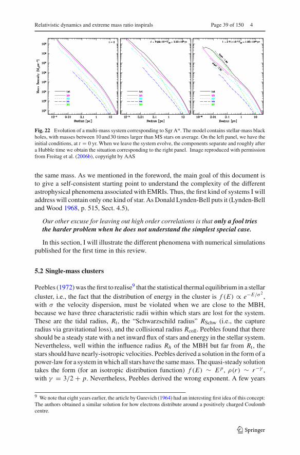
Relativistic dynamics and extreme mass ratio inspirals Page 39 of 150 4
Fig. 22 Evolution of a multi-mass system corresponding to Sgr A*. The model contains stellar-mass blackholes, with masses between 10 and 30 times larger than MS stars on average. On the left panel, we have theinitial conditions, at t = 0 yr. When we leave the system evolve, the components separate and roughly aftera Hubble time we obtain the situation corresponding to the right panel. Image reproduced with permissionfrom Freitag et al. (2006b), copyright by AAS
the same mass. As we mentioned in the foreword, the main goal of this document isto give a self-consistent starting point to understand the complexity of the differentastrophysical phenomena associated with EMRIs. Thus, the first kind of systems I willaddress will contain only one kind of star. As Donald Lynden-Bell puts it (Lynden-Belland Wood 1968, p. 515, Sect. 4.5),
Our other excuse for leaving out high order correlations is that only a fool triesthe harder problem when he does not understand the simplest special case.
In this section, I will illustrate the different phenomena with numerical simulationspublished for the first time in this review.
5.2 Single-mass clusters
Peebles (1972) was the first to realise9 that the statistical thermal equilibrium in a stellarcluster, i.e., the fact that the distribution of energy in the cluster is f (E) ∝ e−E/σ 2
,with σ the velocity dispersion, must be violated when we are close to the MBH,because we have three characteristic radii within which stars are lost for the system.These are the tidal radius, Rt , the “Schwarzschild radius” RSchw (i.e., the captureradius via gravitational loss), and the collisional radius Rcoll. Peebles found that thereshould be a steady state with a net inward flux of stars and energy in the stellar system.Nevertheless, well within the influence radius Rh of the MBH but far from Rt , thestars should have nearly-isotropic velocities. Peebles derived a solution in the form of apower-law for a system in which all stars have the same mass. The quasi-steady solutiontakes the form (for an isotropic distribution function) f (E) ∼ E p, ρ(r) ∼ r−γ ,with γ = 3/2 + p. Nevertheless, Peebles derived the wrong exponent. A few years
9 We note that eight years earlier, the article by Gurevich (1964) had an interesting first idea of this concept:The authors obtained a similar solution for how electrons distribute around a positively charged Coulombcentre.
123

4 Page 40 of 150 P. Amaro-Seoane
later, Bahcall and Wolf (1976) did an exhaustive kinematic treatment for single-masssystems and found that the exponent should be γ = 7/4 and p = γ − 3/2 = 1/4.This solution has been corroborated in a number of semi-/analytical approaches, andapproximative numerical schemes, see e.g., Shapiro and Marchant (1978), Marchantand Shapiro (1979), Marchant and Shapiro (1980), Shapiro and Teukolsky (1985),Freitag and Benz (2001), Amaro-Seoane et al. (2004), as well as direct-summationN -body simulations, of which the work of Preto et al. (2004) was the first one.
This is one of the most important phenomena in the production of EMRIs, since thegalactic nuclei of interest for us, the ones which are thought to be harbouring EMRIs intheir cores and are in the range of frequencies of interest, are relaxed. These nuclei arerelatively small and are likely to have at least gone through at least one full relaxationtime. In general, nuclei in the range of interest for LISA are relaxed (see the rule ofthumb introduced in Preto 2010).
5.3 Mass segregation in two mass-component clusters
As we have just seen, the processes that one-component clusters bring about arenowadays relatively well understood and has been plentifully studied by differentauthors to check for the quality of their approaches. Nonetheless, the properties ofmulti-mass systems are only very poorly represented by idealised models in whichall stars have a single mass. New features of these systems’ behaviour arise when weconsider a stellar system in which masses are divided into two groups. Hence, sincethe idealised situation in which all stars in a stellar cluster have the same mass has beenarduously examined in literature, we have the right to extend the analysis a furtherstep. Here I address more realistic configurations in which the stellar system is splitinto various components. The second integer immediately after one is two, so we willfirst extend, cautious and wary as we are, our models to two-component star clusters.
Initial mass functions (IMFs), introduced with more detail in Sect. 5.4, rangingbetween [0.1, ∼ 120]M� can be approximated to first order by two well-separatedmass scales : one with a mass of the order of O(1M�) (which could represent main-sequence stars, MS, white dwarfs, WD, or neutron stars NS) and O(10M�) (stellar-mass black holes). Depending on how the system taken into consideration is configuredwe will exclude dynamical equilibrium (meaning that the system is not stable ondynamical time-scales) or equipartition of different components kinetic energies isnot allowed (thermal equilibrium).
The work of Spitzer Jr (1969) was in this respect pioneering. For some clusters, itseemed impossible to find a configuration in which they enjoy dynamical and thermalequilibrium together. The heavy components sink into the centre because they cedekinetic energy to the light ones when reaching equipartition. The process will carryon until equipartition is fully gained. In most of the cases, equipartition happens to beimpossible, because the subsystem of massive stars will undergo core collapse beforeequipartiton is reached. Anon, a gravothermal collapse will happen in this componentand, as a result, a small dense core of heavy stars is formed Spitzer Jr (1969), Lightmanand Fall (1978). This gravothermal contraction is a product of negative heat capacity,a typical property of gravitationally bound systems Elson et al. (1987).
123

Relativistic dynamics and extreme mass ratio inspirals Page 41 of 150 4
Different authors have addressed the problem of thermal and dynamical equilibriumin such systems, using techniques such as direct N -body Portegies Zwart and McMillan(2000), Khalisi et al. (2007) and Monte Carlo simulations Watters et al. (2000) todirect integration of the Fokker–Planck equation Inagaki and Wiyanto (1984), Kimet al. (1998) or moments of it Amaro-Seoane et al. (2004), including Monte Carloapproaches to the numerical integration of this equation Spitzer Jr and Hart (1971).For a general and complete overview of the historical evolution of two-stars stellarcomponents, see Watters et al. (2000), Amaro-Seoane et al. (2004) and referencestherein.
If we do not have any energy source in the cluster and stars do not collide (physi-cally), the contraction carries on self-similarly indefinitely; in such a case, one says thatthe system undergoes core collapse. This phenomenon has been observed in a largenumber of works using different methods Hénon (1973); Hénon (1975), Spitzer Jrand Shull (1975), Cohn (1980), Marchant and Shapiro (1980), Stodołkiewicz (1982),Takahashi (1993), Giersz and Heggie (1994), Takahashi (1995), Spurzem and Aarseth(1996), Makino (1996), Quinlan (1996), Drukier et al. (1999), Joshi et al. (2000). Corecollapse is not just a characteristic of multi-mass systems, but has been also observedin single mass analysis.
Spitzer Jr (1969) gives the analytical criterion to determine whether a two-component system has achieved energy equipartition. According to this analysis,energy equipartition between the light and heavy component exists if the followinginequality holds
S :=(Mh
Ml
)(mh
ml
)3/2
< 0.16. (52)
Where Ml and Mh are the total numbers of light and heavy components, respectively(i.e., the total stellar mass in light stars and heavy stars in the system). More numericalcalculations Watters et al. (2000) have settled this criterion to
Λ :=(Mh
Ml
)(mh
ml
)2.4
< 0.16 (53)
When we modify the ratio Mmax/M , the time required to reach core-collapse isdifferent. In a cluster with, for instance, a broad Salpeter initial mass function (IMF)between [0.2 M�, 120 M�], core-collapse takes place after a time � 0.1 trh(0), whilefor a single-mass Plummer model it occurs after a time � 10 trh(0) (this specificexample was taken from the Monte Carlo-based calculations of Gürkan et al. 2004).
There is an ample evidence for mass segregation in observed clusters. McCaughreanand Stauffer (1994) and Hillenbrand and Hartmann (1998) provided deep infraredobservations of the Trapezium cluster in Orion that clearly show the mass segregationin the system, with the highest mass stars segregated into the centre of the cluster. Totest whether there is evidence for more general mass segregation, they showed in a plotreproduced in Fig. 23 cumulative distributions with radius of stars contained withindifferent mass intervals. They include in the figure four different panels in order tomake clear the sensitivity to the limiting radius. They find that, inside 1.0 pc, generalmass segregation appears to be established in the cluster, with stars of masses less
123
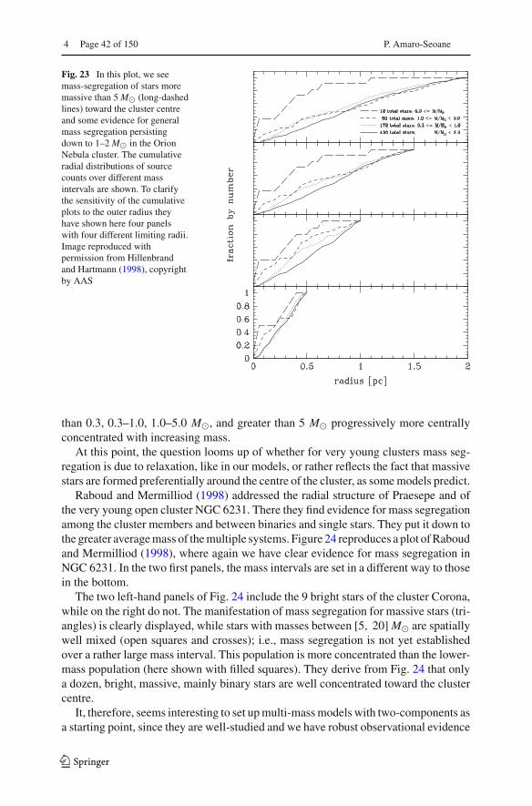
4 Page 42 of 150 P. Amaro-Seoane
Fig. 23 In this plot, we seemass-segregation of stars moremassive than 5 M� (long-dashedlines) toward the cluster centreand some evidence for generalmass segregation persistingdown to 1–2 M� in the OrionNebula cluster. The cumulativeradial distributions of sourcecounts over different massintervals are shown. To clarifythe sensitivity of the cumulativeplots to the outer radius theyhave shown here four panelswith four different limiting radii.Image reproduced withpermission from Hillenbrandand Hartmann (1998), copyrightby AAS
than 0.3, 0.3–1.0, 1.0–5.0 M�, and greater than 5 M� progressively more centrallyconcentrated with increasing mass.
At this point, the question looms up of whether for very young clusters mass seg-regation is due to relaxation, like in our models, or rather reflects the fact that massivestars are formed preferentially around the centre of the cluster, as some models predict.
Raboud and Mermilliod (1998) addressed the radial structure of Praesepe and ofthe very young open cluster NGC 6231. There they find evidence for mass segregationamong the cluster members and between binaries and single stars. They put it down tothe greater average mass of the multiple systems. Figure 24 reproduces a plot of Raboudand Mermilliod (1998), where again we have clear evidence for mass segregation inNGC 6231. In the two first panels, the mass intervals are set in a different way to thosein the bottom.
The two left-hand panels of Fig. 24 include the 9 bright stars of the cluster Corona,while on the right do not. The manifestation of mass segregation for massive stars (tri-angles) is clearly displayed, while stars with masses between [5, 20] M� are spatiallywell mixed (open squares and crosses); i.e., mass segregation is not yet establishedover a rather large mass interval. This population is more concentrated than the lower-mass population (here shown with filled squares). They derive from Fig. 24 that onlya dozen, bright, massive, mainly binary stars are well concentrated toward the clustercentre.
It, therefore, seems interesting to set up multi-mass models with two-components asa starting point, since they are well-studied and we have robust observational evidence
123

Relativistic dynamics and extreme mass ratio inspirals Page 43 of 150 4
Fig. 24 Mass segregation inNGC 623 for two mass intervalsets. The two left panels includeall sample stars, while the rightones do not include the 9 brightstars of the cluster corona. Forthe two top figures M < 5 M�(filled squares),M ∈ [5, 10[ M� (opensquares), M ∈ [10, 20[ M�(crosses) and M ≥ 20 M�(triangles). For the two bottomfigures, M < 2.5 M� (filledsquares), M ∈ [2.5, 6.3[ M�(open squares),M ∈ [6.3, 15.8[ M� (crosses)and M ≥ 15.8 M� (triangles).Image reproduced withpermission from Raboud andMermilliod (1998), copyright byESO
of this phenomenon. On the other hand, observations do not tell us whether masssegregation is due to relaxation. I now show the results from a set of 104 simulationsfor two-component models using the “Gaseous Model” programme to illustrate this(see Sect. 8). I define two parameters now that describe the physics of the system,
q := Mh/M ,
μ := mh/ml (54)
In this definition, M is the total mass of the system, Mh the total mass in heavy starsand mh, l the mass of one heavy (light) star. In the expression, q is the total stellarmass in heavy stars normalised to the total mass of the system, and μ the mass ratiobetween heavy and light stars.
Now, I introduce the quantity ζ ≡ 1−q, and we let ζ vary from 10−4 to 9.99 ·10−1.For each ζ value, we let μ vary between 1.03 and 103. The values for q are regularlydistributed in log (ζ ). For ζ ≈ 1 we have added a series of values in log (ζ − 1).The mean particle mass is 1, M� and the total mass 106 M�, but this is not importantfor our study, because the physics of the system is driven by relaxation and thereforethe only relevant concept is the relaxation time. We can always extend the physics toany other system containing more particles, with the proviso that only relaxation isat play. The mean mass is therefore just a normalisation. What really determines thedynamics of the system are the mass ratios, q and μ, which is the reason why I usethem to explore the system.
In Fig. 25, I show the whole (q, μ)-parameter space in a plot where the time atwhich the core-collapse begins is included. The green zone corresponds to the quasisingle-mass case. In the red zone we have the largest difference between masses andblue is an intermediate case.
123
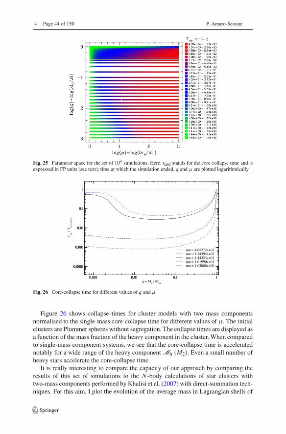
4 Page 44 of 150 P. Amaro-Seoane
Fig. 25 Parameter space for the set of 104 simulations. Here, tend stands for the core collapse time and isexpressed in FP units (see text); time at which the simulation ended. q and μ are plotted logarithmically
11.010.0100.0q = M
h / M
tot
0.0001
0.001
0.01
0.1
1
Tcc
/ T
cc (
s.m
.)
11.010.0100.0
0.0001
0.001
0.01
0.1
1
mu = 4.05272e+02mu = 1.24394e+02mu = 1.44353e+01mu = 1.01990e+01mu = 1.03000e+00
Fig. 26 Core-collapse time for different values of q and μ
Figure 26 shows collapse times for cluster models with two mass componentsnormalised to the single-mass core-collapse time for different values of μ. The initialclusters are Plummer spheres without segregation. The collapse times are displayed asa function of the mass fraction of the heavy component in the cluster. When comparedto single-mass component systems, we see that the core-collapse time is acceleratednotably for a wide range of the heavy component Mh (M2). Even a small number ofheavy stars accelerate the core-collapse time.
It is really interesting to compare the capacity of our approach by comparing theresults of this set of simulations to the N -body calculations of star clusters withtwo-mass components performed by Khalisi et al. (2007) with direct-summation tech-niques. For this aim, I plot the evolution of the average mass in Lagrangian shells of
123

Relativistic dynamics and extreme mass ratio inspirals Page 45 of 150 4
Fig. 27 Average mass inLagrangian shells from averagedmass in Lagrangian spheres
m_
(i+1)
*
m_
(i)*
m*_ (i; i+1)
M(i)r
(i+1)M r
the cluster from the averaged mass in Lagrangian spheres containing the followingmass percentages [0–1], [2–5], [10–20], [40–50], [75–95]%, among others, to be ableto compare with the results of Khalisi et al. (2007). These are the comprised volumebetween two Lagrangian radii, which contain a fixed mass fraction of the bound starsin the system.
We have calculated the average mass as follows: If M (i)r is the total mass for the
component i comprised at the radius r and m(i)� is the average mass for this component
within that radius, we can find out what is the value of m(i; i+1)� (the average mass
between m(i)� and m(i+1)
� ) knowing M (i)r , M (i+1)
r , m(i)� and m(i+1)
� . This is schematicallyshown in Fig. 27. Indeed,
M (i+1)r = N (i)
r · m(i)� + N (i; i+1)
r · m(i; i+1)� = N (i+1)
r · m(i+1)� . (55)
SinceN (i+1)
r = N (i)r + N (i; i+1)
r , (56)
where
N (i)r = M (i)
r
m(i)�
(57)
we have that, from Eq. (55),
m(i; i+1)� = M (i+1)
r − M (i)r
M(i+1)r
m(i+1)�
− M(i)r
m(i)�
(58)
123
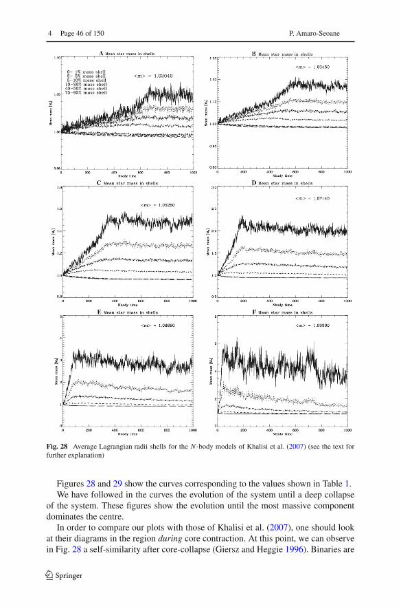
4 Page 46 of 150 P. Amaro-Seoane
Fig. 28 Average Lagrangian radii shells for the N -body models of Khalisi et al. (2007) (see the text forfurther explanation)
Figures 28 and 29 show the curves corresponding to the values shown in Table 1.We have followed in the curves the evolution of the system until a deep collapse
of the system. These figures show the evolution until the most massive componentdominates the centre.
In order to compare our plots with those of Khalisi et al. (2007), one should lookat their diagrams in the region during core contraction. At this point, we can observein Fig. 28 a self-similarity after core-collapse (Giersz and Heggie 1996). Binaries are
123

Relativistic dynamics and extreme mass ratio inspirals Page 47 of 150 4
μ = 1.27 μ = 1.56
μ = 2.06 μ = 2.92
μ = 5.09 μ = 10.2
Fig. 29 Average Lagrangian radii shells for our models, equivalent to those of Fig. 28
123
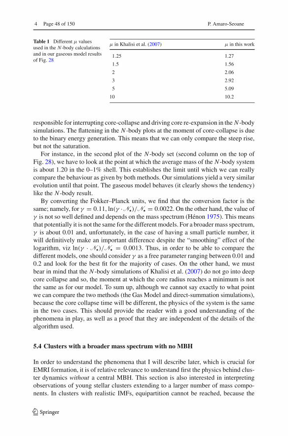
4 Page 48 of 150 P. Amaro-Seoane
Table 1 Different μ valuesused in the N -body calculationsand in our gaseous model resultsof Fig. 28
μ in Khalisi et al. (2007) μ in this work
1.25 1.27
1.5 1.56
2 2.06
3 2.92
5 5.09
10 10.2
responsible for interrupting core-collapse and driving core re-expansion in the N -bodysimulations. The flattening in the N -body plots at the moment of core-collapse is dueto the binary energy generation. This means that we can only compare the steep rise,but not the saturation.
For instance, in the second plot of the N -body set (second column on the top ofFig. 28), we have to look at the point at which the average mass of the N -body systemis about 1.20 in the 0–1% shell. This establishes the limit until which we can reallycompare the behaviour as given by both methods. Our simulations yield a very similarevolution until that point. The gaseous model behaves (it clearly shows the tendency)like the N -body result.
By converting the Fokker–Planck units, we find that the conversion factor is thesame; namely, for γ = 0.11, ln(γ ·N�)/N� = 0.0022. On the other hand, the value ofγ is not so well defined and depends on the mass spectrum (Hénon 1975). This meansthat potentially it is not the same for the different models. For a broader mass spectrum,γ is about 0.01 and, unfortunately, in the case of having a small particle number, itwill definitively make an important difference despite the “smoothing” effect of thelogarithm, viz ln(γ · N�)/N� = 0.0013. Thus, in order to be able to compare thedifferent models, one should consider γ as a free parameter ranging between 0.01 and0.2 and look for the best fit for the majority of cases. On the other hand, we mustbear in mind that the N -body simulations of Khalisi et al. (2007) do not go into deepcore collapse and so, the moment at which the core radius reaches a minimum is notthe same as for our model. To sum up, although we cannot say exactly to what pointwe can compare the two methods (the Gas Model and direct-summation simulations),because the core collapse time will be different, the physics of the system is the samein the two cases. This should provide the reader with a good understanding of thephenomena in play, as well as a proof that they are independent of the details of thealgorithm used.
5.4 Clusters with a broader mass spectrum with no MBH
In order to understand the phenomena that I will describe later, which is crucial forEMRI formation, it is of relative relevance to understand first the physics behind clus-ter dynamics without a central MBH. This section is also interested in interpretingobservations of young stellar clusters extending to a larger number of mass compo-nents. In clusters with realistic IMFs, equipartition cannot be reached, because the
123

Relativistic dynamics and extreme mass ratio inspirals Page 49 of 150 4
most massive stars build a subsystem in the cluster’s centre as the process of segrega-tion goes on thanks to the kinetic energy transfer to the light mass components until thecluster undergoes core collapse (Spitzer Jr 1969; Inagaki and Wiyanto 1984; Inagakiand Saslaw 1985). Although the case in which the MBH is lurking at the centre ofthe host cluster is more attractive for EMRI production and from a dynamical pointof view, one should study, in a first step, more simple models.
In this section we want, thus, to go a step further and evaluate stellar clusters witha broad mass function (MF hereafter). For this, I will again be using the Gas Model,because it is a good compromise between accuracy and integration time for this review.
We study those clusters for which the relaxation time is relatively short, because themost massive stars will sink to the centre of the system due to mass segregation beforethey have time to leave the main sequence (MS). In this scenario we can consider,as an approximation, that stellar evolution plays no role; stars did not have time tostart evolving. The configuration is similar to that of Gürkan et al. (2004), but theyemploy a rather different approach based on a Monte Carlo code (MC), using theideas of Hénon (1973) that allow one to study various aspects of the stellar dynamicsof a dense stellar cluster with or without a central MBH. Our scheme, although beingmore approximate than MC codes (and direct-summation N -body ones) and unable,in its present version, to account for collision has the advantage, as we will see in theSect. 8, of being much faster to run, and of providing data that has no numerical noise.It captures the essential features of the physical systems considered in our analysis andis an interesting, powerful tool for illustrating the different scenarios in this review.
One of the first questions we should address is the maximum number of componentsone should take into consideration when performing our calculations. Since the com-putational time becomes larger and larger when adding more and more componentsto the system -even for an approximative scheme such as the Gas Model-, we shouldfirst find out what is a realistic number of components in our case. For this end I haveperformed different computations with different number of stellar components.
For the simulations shown here, the initial cluster models are Plummer models witha Salpeter IMF (Salpeter 1955),
dN�
dM�
∝ M−α� (59)
between 0.2 and 120 M�. In this equation α = 2.35. There is no initial mass segrega-tion. The discretisation of the mass components follows this recipe:
log(Mcomp|i ) = log(Mmin) + log
(Mmax
Mmin
)·(
i
Ncomp+1
)δ
(60)
In this equation, δ is the discretisation exponent. If δ > 1 we have more bins atlow mass; for δ < 1, we have more bins at high mass. That is, δ allows one to putmore discretised mass components at low masses (δ > 1) or at high masses (δ < 1),δ = 1 gives the logarithmical equal spacing. Mmax,min are, respectively, the maximumand minimum individual stellar masses for the components. For all simulations that Ipresent, the number of mass bins has been typically set to 15. I have chosen a Plummer
123
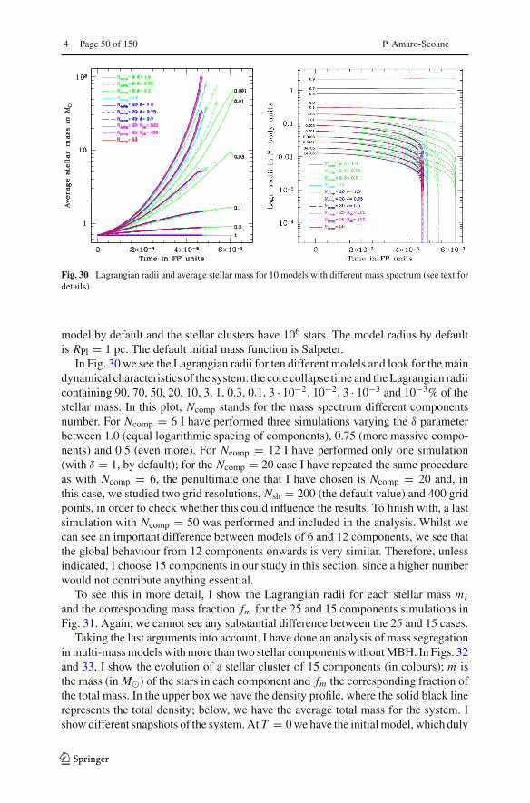
4 Page 50 of 150 P. Amaro-Seoane
Fig. 30 Lagrangian radii and average stellar mass for 10 models with different mass spectrum (see text fordetails)
model by default and the stellar clusters have 106 stars. The model radius by defaultis RPl = 1 pc. The default initial mass function is Salpeter.
In Fig. 30 we see the Lagrangian radii for ten different models and look for the maindynamical characteristics of the system: the core collapse time and the Lagrangian radiicontaining 90, 70, 50, 20, 10, 3, 1, 0.3, 0.1, 3 · 10−2, 10−2, 3 · 10−3 and 10−3% of thestellar mass. In this plot, Ncomp stands for the mass spectrum different componentsnumber. For Ncomp = 6 I have performed three simulations varying the δ parameterbetween 1.0 (equal logarithmic spacing of components), 0.75 (more massive compo-nents) and 0.5 (even more). For Ncomp = 12 I have performed only one simulation(with δ = 1, by default); for the Ncomp = 20 case I have repeated the same procedureas with Ncomp = 6, the penultimate one that I have chosen is Ncomp = 20 and, inthis case, we studied two grid resolutions, Nsh = 200 (the default value) and 400 gridpoints, in order to check whether this could influence the results. To finish with, a lastsimulation with Ncomp = 50 was performed and included in the analysis. Whilst wecan see an important difference between models of 6 and 12 components, we see thatthe global behaviour from 12 components onwards is very similar. Therefore, unlessindicated, I choose 15 components in our study in this section, since a higher numberwould not contribute anything essential.
To see this in more detail, I show the Lagrangian radii for each stellar mass mi
and the corresponding mass fraction fm for the 25 and 15 components simulations inFig. 31. Again, we cannot see any substantial difference between the 25 and 15 cases.
Taking the last arguments into account, I have done an analysis of mass segregationin multi-mass models with more than two stellar components without MBH. In Figs. 32and 33, I show the evolution of a stellar cluster of 15 components (in colours); m isthe mass (in M�) of the stars in each component and fm the corresponding fraction ofthe total mass. In the upper box we have the density profile, where the solid black linerepresents the total density; below, we have the average total mass for the system. Ishow different snapshots of the system. At T = 0 we have the initial model, which duly
123

Relativistic dynamics and extreme mass ratio inspirals Page 51 of 150 4
Fig. 31 Lagrangian radii for each stellar mass mi for the cases of 25 and 15 mass components
Fig. 32 Initial density profile for a stellar cluster with 15 components (upper panel) in N -body units andaverage total stellar mass in M� (lower panel)
shows no mass segregation. As time passes, at T = 5.30 ·10−2 Trh(0), with Trh(0) thevalue of Trh at the beginning of the simulation, we observe how mass segregation hasfragmented the initial configuration; the heavy components have sunk into the centralregions of the stellar cluster and, thus, increased the mean average mass. The outerparts of the system start losing their heavy stars quickly and, consequently, their densityprofile decreases. This becomes more acute for later times at T = 6.75 · 10−2 Trh(0),
123

4 Page 52 of 150 P. Amaro-Seoane
Fig. 33 Same situation as in Fig. 32 but at later times. See text for explanations
as the plots on the right in Fig. 33 show. In these plots and, more clearly in the rightpanel of density profile, we can observe a depletion at intermediate radii.
5.5 Core-collapse evolution
Gürkan et al. (2004) show that for a broad MF—either Salpeter or Kroupa—, masssegregation produces a core-collapse of the system that happens very fast. For clustersof moderate initial concentration, they find that this happens in about 10% of the Trh(0),the initial half-mass relaxation time (i.e., the half-relaxation time that the cluster hadwhen time started, at t = 0). A good and clear illustration of this is Figs. 34 and 35.In the former, on the left panel we have the initial configuration of the system. On theright one, we have the cluster at the moment of core-collapse. In the figure, all starswithin a slice containing the centre have been depicted. On the other hand, this doesnot represent a real physical system, because all radii have been magnified (see thebottom of each panel). The dashed circles represent spheres containing 1, 3 and 10 %of the total cluster mass (from the centre). We can clearly see how the massive, largestars are segregated towards the centre. In Fig. 35, I show the core-collapse evolutionof a multi-mass stellar cluster simulated with the gaseous model. As usual, m is themass (in M�) of the stars in each component and fm the corresponding fraction ofthe total mass. On the left panel I display the time evolution of the central density fora model in which I have employed 15 individual mass components. The total densityis given by the dotted line. On the right panel we have the evolution of the centralvelocity dispersions. The dotted black line shows the mass-averaged value
σ 2 =√∑15
i=1 mi σ2i
m, (61)
and I use N -body units for the y-axes.
123
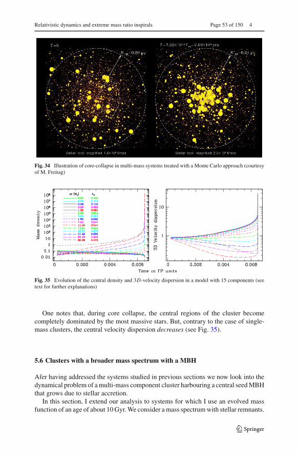
Relativistic dynamics and extreme mass ratio inspirals Page 53 of 150 4
Fig. 34 Illustration of core-collapse in multi-mass systems treated with a Monte Carlo approach (courtesyof M. Freitag)
Fig. 35 Evolution of the central density and 3D-velocity dispersion in a model with 15 components (seetext for further explanations)
One notes that, during core collapse, the central regions of the cluster becomecompletely dominated by the most massive stars. But, contrary to the case of single-mass clusters, the central velocity dispersion decreases (see Fig. 35).
5.6 Clusters with a broader mass spectrum with a MBH
Afer having addressed the systems studied in previous sections we now look into thedynamical problem of a multi-mass component cluster harbouring a central seed MBHthat grows due to stellar accretion.
In this section, I extend our analysis to systems for which I use an evolved massfunction of an age of about 10 Gyr. We consider a mass spectrum with stellar remnants.
123
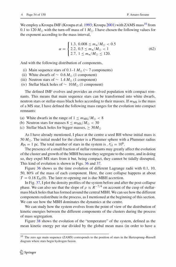
4 Page 54 of 150 P. Amaro-Seoane
We employ a Kroupa IMF (Kroupa et al. 1993; Kroupa 2001) with ZAMS mass10 from0.1 to 120 M� with the turn-off mass of 1 M�. I have chosen the following values forthe exponent according to the mass interval,
α =⎧⎨⎩
1.3, 0.008 ≤ m�/M� < 0.52.2, 0.5 ≤ m�/M� < 12.7, 1 ≤ m�/M� ≤ 120.
(62)
And with the following distribution of components,
(i) Main sequence stars of 0.1–1 M� (∼ 7 components)(ii) White dwarfs of ∼ 0.6 M� (1 component)
(iii) Neutron stars of ∼ 1.4 M� (1 component)(iv) Stellar black holes of ∼ 10M� (1 component)
The defined IMF evolves and provides an evolved population with compact rem-nants. This means that main sequence stars can be transformed into white dwarfs,neutron stars or stellar-mass black holes according to their masses. If mMS is the massof a MS star, I have defined the following mass ranges for the evolution into compactremnants:
(a) White dwarfs in the range of 1 ≤ mMS/M� < 8(b) Neutron stars for masses 8 ≤ mMS/M� < 30(c) Stellar black holes for bigger masses, ≥ 30M�
As I have already mentioned, I place at the centre a seed BH whose initial mass is50 M�. The initial model for the cluster is a Plummer sphere with a Plummer radiusRPl = 1 pc. The total number of stars in the system is Ncl = 106.
The presence of a small fraction of stellar remnants may greatly affect the evolutionof the cluster and growth of the MBH because they segregate to the centre, and in doingso, they expel MS stars from it but, being compact, they cannot be tidally disrupted.This kind of evolution is shown in Figs. 36 and 37.
Figure 36 shows us the time evolution of different Lagrange radii with 0.1, 10,50, 80% of the mass of each component. Here, the core collapse happens at aboutT = 0.18 Trh(0). The later re-opening out is due MBH accretion.
In Fig. 37, I plot the density profiles of the system before and after the post-collapsephase. We can also see that the slope of ρ ∝ R−7/4 on account of the cusp of stellar-mass black holes that has formed around the central MBH. We can see how the differentcomponents redistribute in the process, as I mentioned at the beginning of this section.We can see how the MBH dominates the dynamics at the centre.
We can study how the system evolves from the point of view of the distribution ofkinetic energies between the different components of the clusters during the processof mass segregation.
Figure 38 shows the evolution of the “temperature” of the system, defined as themean kinetic energy per star divided by the global mean mass (in order to have a
10 The zero age main sequence (ZAMS) corresponds to the position of stars in the Hertzsprung–Russelldiagram where stars begin hydrogen fusion.
123
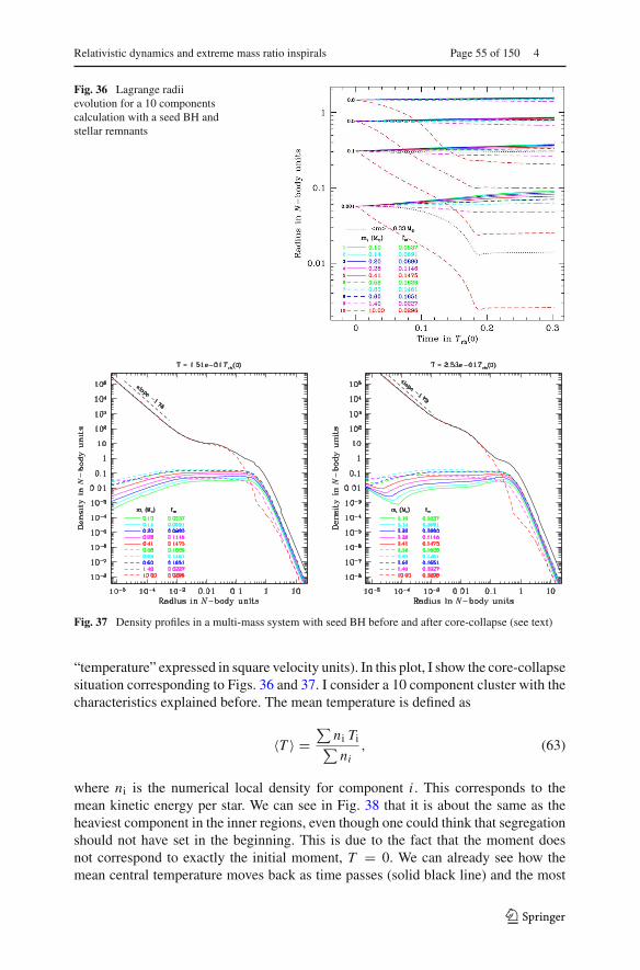
Relativistic dynamics and extreme mass ratio inspirals Page 55 of 150 4
Fig. 36 Lagrange radiievolution for a 10 componentscalculation with a seed BH andstellar remnants
Fig. 37 Density profiles in a multi-mass system with seed BH before and after core-collapse (see text)
“temperature” expressed in square velocity units). In this plot, I show the core-collapsesituation corresponding to Figs. 36 and 37. I consider a 10 component cluster with thecharacteristics explained before. The mean temperature is defined as
〈T 〉 =∑
ni Ti∑ni
, (63)
where ni is the numerical local density for component i . This corresponds to themean kinetic energy per star. We can see in Fig. 38 that it is about the same as theheaviest component in the inner regions, even though one could think that segregationshould not have set in the beginning. This is due to the fact that the moment doesnot correspond to exactly the initial moment, T = 0. We can already see how themean central temperature moves back as time passes (solid black line) and the most
123

4 Page 56 of 150 P. Amaro-Seoane
Fig. 38 Different moments in the evolution of the cluster temperature for a 10 stellar components systemwith a seed MBH
massive component (dashed red line) increases. For later times, the kinetic energies ofthe different components rise at the inner part of the cluster and the most massive oneapproaches the sum of all of them. This is even more evident in the last plot, where thetemperatures of all components sink except for that corresponding to the most massiveone.
6 Two-body extreme mass ratio inspirals
After the first sections we have a good understanding of the fundamentals of two-bodyrelaxation in dense stellar systems, including mass segregation and dynamical friction,which could be roughly described as “relaxation when we have a large mass ratio”.In this section, I address the subject of capture of compact objects by a massive blackhole considering that the driving mechanism in the production is two-body relaxation.
123

Relativistic dynamics and extreme mass ratio inspirals Page 57 of 150 4
6.1 A hidden stellar population in galactic nuclei
The question about the distribution and capture of stellar-mass black holes at the Galac-tic Centre has been addressed a number of times by different authors, from both a semi-or analytical and numerical standpoint, see e.g., Sigurdsson and Rees (1997), Miralda-Escudé and Gould (2000), Freitag (2001, 2003b), Freitag et al. (2006a, b), Hopmanand Alexander (2006b), Amaro-Seoane et al. (2007), Preto and Amaro-Seoane (2010),Amaro-Seoane and Preto (2011). Addressing this problem has implications for a vari-ety of astrophysical questions, including of course inspirals of compact objects ontothe central MBH, but also on the distribution of X-ray binaries at the Galactic Centre,tidal disruptions of main sequence stars, and the behaviours of the so-called “source”stars, which were introduced in Sect. 2.2. Even if we only consider single stellar-massblack holes, the impact they can have on the S-stars is not negligible; a distributionof non-luminous matter around the Galactic Centre would have a clear fingerprint ontheir orbits. Current data are insufficient to detect such an extended non-luminous cuspwhich typically would induce a slight Newtonian retrograde precession (Mouawadet al. 2005), so that we will have to wait for future telescopes before we can hopeto see such trajectory deflections. The study of Weinberg et al. (2005) estimated thatproposed 30–100 m aperture telescopes will allow us to observe about three trajectorydeflections per year between any of the monitored “source” stars and a stellar-massblack hole.
The centermost part of the stellar spheroid, the galactic nucleus, constitutesan extreme environment for stellar dynamics. With stellar densities higher than106 M� pc−3, relative velocities in excess of 100 km s−1 the nucleus (unlike mostof the rest of the galaxy) is the site of a variety of “collisional processes”—bothclose encounters and actual collisions between stars, as we have seen in the previoussections. The central MBH and the surrounding stellar environment interact throughvarious mechanisms: some are global, like the accretion of gases liberated by stel-lar evolution or the adiabatic adaptation of stellar orbits as the mass of the MBHincreases; others, which involve the close interaction between a star and the MBH—EMRIs and stellar disruptions—are local in nature. As we have seen in Sect. 4.4, tointeract closely with the central MBH, stars have to find themselves on “loss-cone”orbits, which are orbits elongated enough to have a very close-in periapsis (Frank andRees 1976; Lightman and Shapiro 1977; Amaro-Seoane and Spurzem 2001).
The rate of tidal disruptions can be established (semi-)analytically if the phasespace distribution of stars around the MBH is known, see Magorrian and Tremaine(1999), Syer and Ulmer (1999), Wang and Merritt (2004) for estimates in models ofobserved nearby nuclei. However, in order to account for the complex influence of masssegregation, collisions and the evolution of the nucleus over billions of years, detailednumerical simulations are required, as in the work of David et al. (1987a, b), Mur-phy et al. (1991), Freitag and Benz (2002), Baumgardt et al. (2004b), Freitag et al.(2006b), Khalisi et al. (2007), Preto and Amaro-Seoane (2010), Amaro-Seoane andPreto (2011).
In the case of a gradual inspiral following the “capture” of a compact object (i.e.,an EMRI), the situation becomes even more complex, even in the idealised case of aspherical nucleus with stars all of the same mass. As the star spirals down towards the
123
4 Page 58 of 150 P. Amaro-Seoane
MBH, it has many opportunities to be deflected back by two-body encounters on toa “safer orbit”, i.e., an orbit which does not lead to gravitational capture (Alexanderand Hopman 2003) hence even the definition of a loss-cone is not straightforward.Once again, the problem is a compound of the effects of mass segregation, generalrelativity and resonant relaxation, to mention three main complications. As as result,considerable uncertainties are attached to the (semi-)analytical predictions of capturerates and orbital parameters of EMRIs.
Only self-consistent stellar dynamical modeling of galactic nuclei will provide uswith a better understanding of these questions. Some steps in that direction have beenmade by Freitag (2001, 2003a, b) using Monte Carlo simulations. Later, Freitag et al.(2006a, b) improved upon these results. Yet these studies neglected a direct estimationof EMRIs or “direct plunges”, due in part to the fact that, to follow stars on veryeccentric orbits, one needs the combined effects of GW emission and relaxation ontimescales much shorter than the capabilities of the numerical Monte Carlo code.Much work remains to be done to confirm these results and improve on them witha more accurate treatment of the physics, to extend them to a larger domain of theparameter space and to more general situations, including non-spherical nuclei.
Classical studies based on approximate stellar dynamics methods that neglect, inparticular, the motion of the central MBH and strong 2-body interactions, indicate that,in dense enough clusters, a “seed” MBH (in the IMBH mass range) could swallowa significant fraction of the cluster mass, and thus become a MBH over the spanof a few Gyrs (Murphy et al. 1991; Freitag and Benz 2002; Amaro-Seoane et al.2004). More detailed, higher fidelity N -body simulations of relatively small clusters(Baumgardt et al. 2004a, b) have not confirmed this classical result, calling for a criticalre-examination and improvement of approximation techniques, the only ones that cancope with the high particle numbers found in massive clusters such as galactic nuclei.It has also been suggested that some processes, such as the effects of chaotic orbits ina slightly non-spherical potential, may effectively keep the loss-cone orbits populated.In this case disruptions and captures can efficiently feed the central MBH and producethe M − σ relation (Zhao et al. 2002; Merritt and Poon 2004).
Understanding the astrophysical processes within galacto-centric clusters that giverise to EMRI events has significant bearing on LISA’s applicability to this science.Accurate predictions of the event rate are important for preparing LISA data anal-ysis and design —many events lead to source-confusion, which must be dealt with,while a few events necessitate identifying weak sources in the presence of instrumen-tal noise (Amaro-Seoane et al. 2007). More importantly, LISA observations alonecannot decouple the mass distribution of the galactic black hole population from themass-dependence of the EMRI rate within a single system. If we can improve ourunderstanding of the latter, we improve LISA’s utility as a probe of the former. Inthis section I elaborate in detail on the “standard” physics leading to sources of grav-itational radiation in the millihertz regime—i.e., in the bandwidth of a LISA-likedetector—originating in two-body relaxation processes.
123
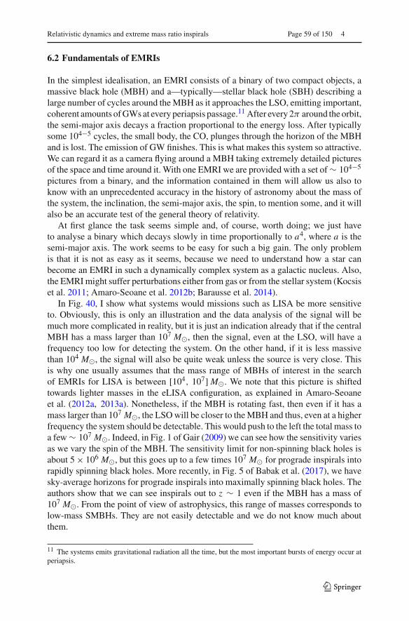
Relativistic dynamics and extreme mass ratio inspirals Page 59 of 150 4
6.2 Fundamentals of EMRIs
In the simplest idealisation, an EMRI consists of a binary of two compact objects, amassive black hole (MBH) and a—typically—stellar black hole (SBH) describing alarge number of cycles around the MBH as it approaches the LSO, emitting important,coherent amounts of GWs at every periapsis passage.11 After every 2π around the orbit,the semi-major axis decays a fraction proportional to the energy loss. After typicallysome 104−5 cycles, the small body, the CO, plunges through the horizon of the MBHand is lost. The emission of GW finishes. This is what makes this system so attractive.We can regard it as a camera flying around a MBH taking extremely detailed picturesof the space and time around it. With one EMRI we are provided with a set of ∼ 104−5
pictures from a binary, and the information contained in them will allow us also toknow with an unprecedented accuracy in the history of astronomy about the mass ofthe system, the inclination, the semi-major axis, the spin, to mention some, and it willalso be an accurate test of the general theory of relativity.
At first glance the task seems simple and, of course, worth doing; we just haveto analyse a binary which decays slowly in time proportionally to a4, where a is thesemi-major axis. The work seems to be easy for such a big gain. The only problemis that it is not as easy as it seems, because we need to understand how a star canbecome an EMRI in such a dynamically complex system as a galactic nucleus. Also,the EMRI might suffer perturbations either from gas or from the stellar system (Kocsiset al. 2011; Amaro-Seoane et al. 2012b; Barausse et al. 2014).
In Fig. 40, I show what systems would missions such as LISA be more sensitiveto. Obviously, this is only an illustration and the data analysis of the signal will bemuch more complicated in reality, but it is just an indication already that if the centralMBH has a mass larger than 107 M�, then the signal, even at the LSO, will have afrequency too low for detecting the system. On the other hand, if it is less massivethan 104 M�, the signal will also be quite weak unless the source is very close. Thisis why one usually assumes that the mass range of MBHs of interest in the searchof EMRIs for LISA is between [104, 107] M�. We note that this picture is shiftedtowards lighter masses in the eLISA configuration, as explained in Amaro-Seoaneet al. (2012a, 2013a). Nonetheless, if the MBH is rotating fast, then even if it has amass larger than 107 M�, the LSO will be closer to the MBH and thus, even at a higherfrequency the system should be detectable. This would push to the left the total mass toa few ∼ 107 M�. Indeed, in Fig. 1 of Gair (2009) we can see how the sensitivity variesas we vary the spin of the MBH. The sensitivity limit for non-spinning black holes isabout 5 × 10⁶ M�, but this goes up to a few times 107 M� for prograde inspirals intorapidly spinning black holes. More recently, in Fig. 5 of Babak et al. (2017), we havesky-average horizons for prograde inspirals into maximally spinning black holes. Theauthors show that we can see inspirals out to z ∼ 1 even if the MBH has a mass of107 M�. From the point of view of astrophysics, this range of masses corresponds tolow-mass SMBHs. They are not easily detectable and we do not know much aboutthem.
11 The systems emits gravitational radiation all the time, but the most important bursts of energy occur atperiapsis.
123

4 Page 60 of 150 P. Amaro-Seoane
Fig. 39 Frequency of a binaryof total mass M1 + M2 againsttheir semi-major axis and thecorresponding frequencies. Thesolid, dark straight line delimitsthe LSO, so that anything on theright of that line is of no interestfor our purposes
Fig. 40 LISA’s sensitivitywindow and four EMRI signals.The groups of colour correspondto the 1st, 2nd and 3rd harmonicin the quadrupole approximationof Peters (1964) for a SBH of10 M� inspiralling on to a MBHof mass 107 M� (cyan, left“cascade” of harmonics),106 M� (blue, second groupfrom the left), 105 M� (orange,third cascade) and and 104 M�(red cascade, first from theright). In each case, the distanceto the source has been set up to1 Gpc M• = 104 M�
m• = 10M�
M• = 107 M�
M• = 105 M�
M• = 106 M�
A different way of looking at the same picture is Fig. 39. I depict, as a function of thetotal, non-redshifted mass of the binary M1 + M2, the semi-major axis of the binaryassuming zero eccentricity. We note here that, even if for some particular models,LISA can in principle detect EMRIs out to a redshift of ∼ 4 (see Babak et al. 2017)most EMRIs will very likely originate from within z ∼ 1, so that for the rest of thiswork I neglect it. In Fig. 39 I show the orbital frequency of the binary. Obviously,for the binary to be in the LISA band, it has to have a frequency of roughly—beinggenerous—between 1 and 10−5 Hz. The emission of GWs is more efficient as theyapproach the LSO, so that LISA will detect the sources when they are close to theLSO line. For masses larger than 107 M� the frequencies even close to the LSO willbe too low, so that their detection will be very difficult. On the other hand, for a totalmass of less than 103 M� in principal we could detect them at an early stage butthen the amplitude of the GWs would be rather low. On top of that, the existence ofintermediate-mass black holes is uncertain.
123

Relativistic dynamics and extreme mass ratio inspirals Page 61 of 150 4
In a spherical potential, at any given time, the stars and compact objects in thenucleus simply orbit the MBH with their semi-major axes and eccentricities changingslowly, owing to 2-body relaxation. For an EMRI to occur, in this standard picture,2-body relaxation has to bring a compact remnant on to an orbit with such a smallperiapsis distance that dissipation of energy by emission of GWs becomes significant.
If the object is on a very eccentric orbit but one for which the timescale for passagethrough periapsis, tperi � (1 − e)3/2P , is less than ∼ 104 s, the source will generatebursts of gravitational radiation in the LISA band each time the object passes throughperiapsis. However, such GW signals consist of bursts which can probably not benefitfrom coherent signal processing even if they repeat with a periodicity shorter thanLISA mission duration. Only if they reside at the Milky Way centre is there a non-vanishing probability for LISA to detect such sources (Rubbo et al. 2006; Hopman et al.2007; Berry and Gair 2013). An extra-galactic source is only likely to be detectableif it radiates continuously in the LISA band. As a rough guide, therefore, a detectableEMRI source must have an orbital frequency higher than about fLISA = 10−4 Hz,corresponding to the condition on the semi-major axis
a � 0.5 AU
(fLISA
10−4 Hz
)−2/3 ( M•106 M�
)1/3
. (64)
As there is no sharp cut-off in the predicted LISA sensitivity curve at 10−4 Hz, astrong source might be detectable at a lower frequency.
Not all objects with an inspiral time by GW emission shorter than a Hubble time willend up as EMRIs. This is because, although relaxation can increase the eccentricity ofan object to very high values, it can also perturb the orbit back to a more circular onefor which GW emission is completely negligible. Typically, neglecting GW emission,it takes a time of the order trlx ln(1 − e) for an orbit to reach a (large) eccentricity ethrough the effects of 2-body relaxation. However, the periapsis distance Rp = a(1−e)can be significantly altered by relaxation on a timescale trel,p � (1 − e) trlx, so thecondition for a star to become an EMRI is that it moves onto an orbit for which thetimescale for orbital decay by GW emission, τGW [see Eq. (73)] is sufficiently shorterthan (1 − e) trlx. If the semi-major axis of the orbit is too large, this condition cannotbe obeyed unless the star actually finds itself on an unstable, plunging orbit, withe ≥ epl(a) ≡ 1−4RSchw/a where RSchw is the Schwarzschild radius of the MBH. Thevery short burst of gravitational radiation emitted during a plunge through the horizoncan only be detected if originating from the Galactic centre (Hopman et al. 2007).Coherent integration of the GW signal for > 104 cycles with a frequency in LISAband is required for detection of extragalactic EMRIs. Therefore a central concern inthe determination of EMRI rates is to distinguish between plunges and progressiveinspirals (Hils and Bender 1995; Hopman and Alexander 2005).
The situation for EMRI production in the standard picture is more complicatedthan that of tidal disruptions by the MBH (e.g., Rees 1988; Magorrian and Tremaine1999; Syer and Ulmer 1999; Wang and Merritt 2004) or GW bursts from stars onvery eccentric orbits (Rubbo et al. 2006; Hopman et al. 2007) because these processesrequire a single passage within a well-defined distance Renc from the MBH to be
123
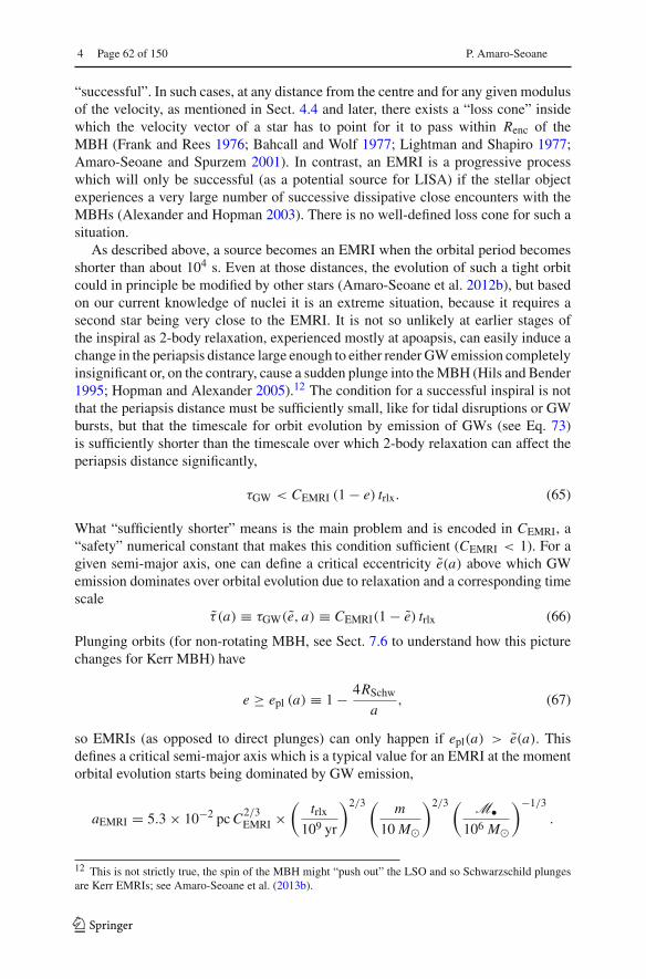
4 Page 62 of 150 P. Amaro-Seoane
“successful”. In such cases, at any distance from the centre and for any given modulusof the velocity, as mentioned in Sect. 4.4 and later, there exists a “loss cone” insidewhich the velocity vector of a star has to point for it to pass within Renc of theMBH (Frank and Rees 1976; Bahcall and Wolf 1977; Lightman and Shapiro 1977;Amaro-Seoane and Spurzem 2001). In contrast, an EMRI is a progressive processwhich will only be successful (as a potential source for LISA) if the stellar objectexperiences a very large number of successive dissipative close encounters with theMBHs (Alexander and Hopman 2003). There is no well-defined loss cone for such asituation.
As described above, a source becomes an EMRI when the orbital period becomesshorter than about 104 s. Even at those distances, the evolution of such a tight orbitcould in principle be modified by other stars (Amaro-Seoane et al. 2012b), but basedon our current knowledge of nuclei it is an extreme situation, because it requires asecond star being very close to the EMRI. It is not so unlikely at earlier stages ofthe inspiral as 2-body relaxation, experienced mostly at apoapsis, can easily induce achange in the periapsis distance large enough to either render GW emission completelyinsignificant or, on the contrary, cause a sudden plunge into the MBH (Hils and Bender1995; Hopman and Alexander 2005).12 The condition for a successful inspiral is notthat the periapsis distance must be sufficiently small, like for tidal disruptions or GWbursts, but that the timescale for orbit evolution by emission of GWs (see Eq. 73)is sufficiently shorter than the timescale over which 2-body relaxation can affect theperiapsis distance significantly,
τGW < CEMRI (1 − e) trlx. (65)
What “sufficiently shorter” means is the main problem and is encoded in CEMRI, a“safety” numerical constant that makes this condition sufficient (CEMRI < 1). For agiven semi-major axis, one can define a critical eccentricity e(a) above which GWemission dominates over orbital evolution due to relaxation and a corresponding timescale
τ (a) ≡ τGW(e, a) ≡ CEMRI(1 − e) trlx (66)
Plunging orbits (for non-rotating MBH, see Sect. 7.6 to understand how this picturechanges for Kerr MBH) have
e ≥ epl (a) ≡ 1 − 4RSchw
a, (67)
so EMRIs (as opposed to direct plunges) can only happen if epl(a) > e(a). Thisdefines a critical semi-major axis which is a typical value for an EMRI at the momentorbital evolution starts being dominated by GW emission,
aEMRI = 5.3 × 10⁻² pcC2/3EMRI ×
(trlx
109 yr
)2/3 ( m
10 M�
)2/3 ( M•106 M�
)−1/3
.
12 This is not strictly true, the spin of the MBH might “push out” the LSO and so Schwarzschild plungesare Kerr EMRIs; see Amaro-Seoane et al. (2013b).
123

Relativistic dynamics and extreme mass ratio inspirals Page 63 of 150 4
The corresponding eccentricity is given by
1 − eEMRI = 7.2 × 10⁻⁶ C−2/3EMRI ×
(trlx
109 yr
)−2/3
×(
m
10 M�
)−2/3 ( M•106 M�
)4/3
.
(68)The situation is represented in Fig. 43 in the semi-major axis—eccentricity plane. I
plot schematically the trajectory for a typical EMRI evolving according to the standardscenario (labelled “1-body inspiral” to distinguish it from the binary tidal separationscenario discussed later). Initially the values of semi-major axis and eccentricity per-form a random walk due to 2-body relaxation. As it takes of the order of trlx to changesemi-major axis by a factor of 2 but only (1 − e)trlx to change the value of 1 − e (andhence the periapsis), the random walk seems more and more elongated in the horizon-tal direction, the smaller the value of 1 − e. It is much more likely for a star to crossover to the plunging or GW-dominated region by acquiring a very high eccentricitythan by shrinking the semi-major axis significantly. Typically, an EMRI “progenitor”starts with a semi-major axis slightly lower than aEMRI. It takes on average a time oforder ln(1 − e)−1trlx � 10trlx for relaxation to produce an eccentricity such that GWemission becomes dominant. From that point, the object will follow a path closer andcloser to a pure inspiral [as approximated by Peters equations (Peters 1964)]. At largersemi-major axis values, inspirals are practically impossible because GW emission isnot significant in comparison to relaxation even on plunge orbits. Unless they firstshrink their orbit through 2-body relaxation, these objects will be swallowed by theMBH on a direct plunge. Inspirals staring with a � aEMRI are rare because, for adensity cusp n ∝ r−α with α � 1.4−1.8 (Baumgardt et al. 2004a, b; Freitag et al.2006b; Hopman and Alexander 2006a), the number of stars per unit log(a) is roughlydN�/d(log a) ∝ a(3−α). Also, as one goes inwards, the value of α is lowered by theprogressively larger plunge loss cone (Lightman and Shapiro 1977; Amaro-Seoaneet al. 2004). In other words, the stellar density is reduced there (in comparison to apure power law) because to come and populate this region a star has to spend severalrelaxation times drifting down in energy while avoiding entering the GW-dominatedregion and inspiraling quickly.
Implementing this basic scenario in various ways (see Sect. 8.7), several authorshave estimated the rate at which stellar remnants are captured by the central MBH,with results between ∼ 10−6 and 10−8 yr−1 for a 106 M� central black hole (Hilsand Bender 1995; Sigurdsson and Rees 1997; Ivanov 2002; Hopman and Alexander2005). When combined with the uncertainty in the number density of massive blackholes with M• < few × 106 M�, the net predicted number of detections that LISAcan make spans over three orders of magnitude, from a few to a few thousand eventsper year.
We note, incidentally, that even in the LISA band (in the final year of inspiral),the eccentricity of the typical EMRI in the standard picture is high enough that alarge number of harmonics are likely to contribute to the gravitational waves (Freitag2003b; Barack and Cutler 2004; Hopman and Alexander 2005). In addition, the orbitalplane of the EMRIs is unlikely to be significantly correlated with the spin plane ofthe MBH. These characteristics are distinct from those in non-standard scenarios
123
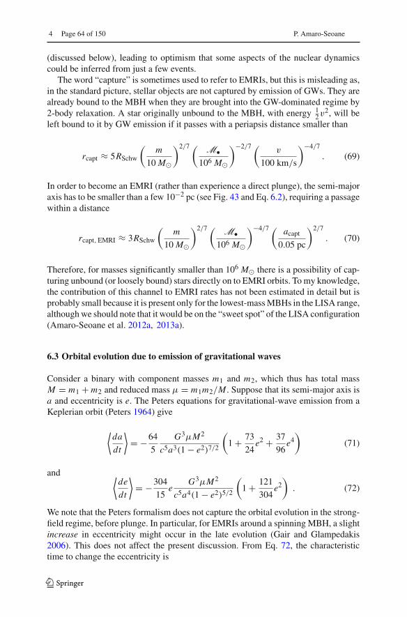
4 Page 64 of 150 P. Amaro-Seoane
(discussed below), leading to optimism that some aspects of the nuclear dynamicscould be inferred from just a few events.
The word “capture” is sometimes used to refer to EMRIs, but this is misleading as,in the standard picture, stellar objects are not captured by emission of GWs. They arealready bound to the MBH when they are brought into the GW-dominated regime by2-body relaxation. A star originally unbound to the MBH, with energy 1
2v2, will beleft bound to it by GW emission if it passes with a periapsis distance smaller than
rcapt ≈ 5RSchw
(m
10 M�
)2/7 ( M•106 M�
)−2/7 (v
100 km/s
)−4/7
. (69)
In order to become an EMRI (rather than experience a direct plunge), the semi-majoraxis has to be smaller than a few 10−2 pc (see Fig. 43 and Eq. 6.2), requiring a passagewithin a distance
rcapt, EMRI ≈ 3RSchw
(m
10 M�
)2/7 ( M•106 M�
)−4/7 ( acapt
0.05 pc
)2/7
. (70)
Therefore, for masses significantly smaller than 106 M� there is a possibility of cap-turing unbound (or loosely bound) stars directly on to EMRI orbits. To my knowledge,the contribution of this channel to EMRI rates has not been estimated in detail but isprobably small because it is present only for the lowest-mass MBHs in the LISA range,although we should note that it would be on the “sweet spot” of the LISA configuration(Amaro-Seoane et al. 2012a, 2013a).
6.3 Orbital evolution due to emission of gravitational waves
Consider a binary with component masses m1 and m2, which thus has total massM = m1 + m2 and reduced mass μ = m1m2/M . Suppose that its semi-major axis isa and eccentricity is e. The Peters equations for gravitational-wave emission from aKeplerian orbit (Peters 1964) give
⟨da
dt
⟩= −64
5
G3μM2
c5a3(1 − e2)7/2
(1 + 73
24e2 + 37
96e4)
(71)
and ⟨de
dt
⟩= −304
15e
G3μM2
c5a4(1 − e2)5/2
(1 + 121
304e2)
. (72)
We note that the Peters formalism does not capture the orbital evolution in the strong-field regime, before plunge. In particular, for EMRIs around a spinning MBH, a slightincrease in eccentricity might occur in the late evolution (Gair and Glampedakis2006). This does not affect the present discussion. From Eq. 72, the characteristictime to change the eccentricity is
123
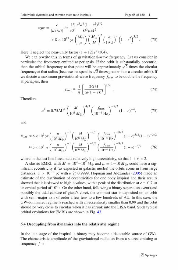
Relativistic dynamics and extreme mass ratio inspirals Page 65 of 150 4
τGW = e
|de/dt | ≈ 15
304
c5a4(1 − e2)5/2
G3μM2
≈ 8 × 10¹⁷ yr
(M�μ
)(M�M
)2 ( a
1AU
)4 (1 − e2
)5/2. (73)
Here, I neglect the near-unity factor (1 + 121e2/304).We can rewrite this in terms of gravitational-wave frequency. Let us consider in
particular the frequency emitted at periapsis. If the orbit is substantially eccentric,then the orbital frequency at that point will be approximately
√2 times the circular
frequency at that radius (because the speed is√
2 times greater than a circular orbit). Ifwe dictate a maximum gravitational-wave frequency fmax to be double the frequencyat periapsis, then
fmax ≈ 1
π
[2GM
(a(1 − e))3
]1/2
. (74)
Therefore
a4 = 0.75AU4(
M
106 M�
)4/3 ( fmax
10−4 Hz
)−8/3
(1 − e)−4, (75)
and
τGW ≈ 6 × 10² yr
(μ
103 M�
)−1 ( M
106 M�
)−2/3 ( fmax
10−4 Hz
)−8/3(1 + e)5/2(1 − e)−3/2
≈ 3 × 10³ yr
(μ
103 M�
)−1 ( M
106 M�
)−2/3 ( fmax
10−4 Hz
)−8/3(1 − e)−3/2 (76)
where in the last line I assume a relatively high eccentricity, so that 1 + e ≈ 2.A classic EMRI, with M = 104−107 M� and μ = 1−10 M�, could have a sig-
nificant eccentricity if (as expected in galactic nuclei) the orbits come in from largedistances, a > 10−2 pc with e � 0.9999. Hopman and Alexander (2005) made anestimate of the distribution of eccentricities for one body inspiral and their resultsshowed that it is skewed to high-e values, with a peak of the distribution at e ∼ 0.7, atan orbital period of 104 s. On the other hand, following a binary separation event (andpossibly the tidal capture of giant’s core), the compact star is deposited on an orbitwith semi-major axis of order a few tens to a few hundreds of AU. In this case, theGW-dominated regime is reached with an eccentricity smaller than 0.99 and the orbitshould be very close to circular when it has shrunk into the LISA band. Such typicalorbital evolutions for EMRIs are shown in Fig. 43.
6.4 Decoupling from dynamics into the relativistic regime
In the late stage of the inspiral, a binary may become a detectable source of GWs.The characteristic amplitude of the gravitational radiation from a source emitting atfrequency f is
123

4 Page 66 of 150 P. Amaro-Seoane
hc = (2E/ f )1/2
πD(77)
where D is the distance to the source, E is the power emitted and f the time derivativeof the frequency (Finn and Thorne 2000). With this definition, the signal-to-noise ratio(SNR) of an event is obtained, assuming ideal signal processing, by the integral13
(SNR)2 =∫ f2
f1
h2c( f )
f Sh( f )d(ln f ) (78)
where f1 and f2 are the initial and final frequencies of the source during the observationand Sh( f ) is the instrumental noise of the detector at frequency f (Phinney 2002;Barack and Cutler 2004).
In Fig. 41, I follow the signal emitted by a binary consisting of a Milky Way-likeMBH and a stellar BH during their GW-driven inspiral without taking into account anypossible dynamical interaction; i.e. we only allow the system to evolve via gravitationalradiation emission. I plot the five lowest harmonics of the quadrupolar emission in arough approximation (Peters and Mathews 1963), only useful for illustrative purposes.In this figure, I assume a distance of 1 Gpc.
For low-eccentric captures only the n = 2 harmonic is detectable, during the lastfew years of inspiral. However, the small residual eccentricity induces a differencein the phase evolution of the n = 2 signal compared to a perfect circular inspiral(Amaro-Seoane and Freitag 2006). If the source is followed from a time τLSO beforemerger until merger, the accumulated phase shift is
Δψe �(e10−4Hz
0.05
)2(
τLSO
1 yr
)17/12 ( Mz
103 M�
)25/36
, (79)
where e10−4Hz is the eccentricity when the n = 2 signal has reached a frequency of10−4 Hz and
Mz ≡ (1 + z)(M•m•)3/5
(M• + m•)1/5(80)
is the redshifted chirp mass of the binary (Cutler and Harms 2006). This means thatin principle we can easily distinguish between high-eccentricity captures and low-eccentricity captures. The implications of this result will become clear in the nextsections.
Figure 43 displays the last stable orbit in the effective Keplerian approximation(Rp � 4 RSchw for e � 0.1, see Cutler et al. (1994) with a solid, thick diagonal line.The thin dotted blue lines are contours of constant time left until the final coalescence,TGW in the Peters (1964) approximation. The years are show on the right. The thindiagonal green lines are the inspiral, capture orbits due only to the emission of GWs.The upper dash-dotted red line shows e(a), defined by te = TGW [Eq. (65) with
13 This is only meant as a very general illustrative description. I refer the reader to Amaro-Seoane et al.(2007), Babak et al. (2010) for a detailed introduction to the problem of detection and parameter estimationof EMRIs.
123

Relativistic dynamics and extreme mass ratio inspirals Page 67 of 150 4
Fig. 41 Characteristic amplitude, introduced in Eq. (77), of the first harmonics of the quadrupolar grav-itational radiation emitted during the inspiral of a stellar-mass BH of m• = 10 M� (m∗ in the plot) intoa MBH of mass M• = 4 × 10⁶ (MBH in the plot). I assume the source is at a distance D = 1 Gpc. Iindicate the noise curve
√f Sh( f ) for a LISA-like detector (Larson et al. 2000; Larson 2003), with the
Galactic binary white dwarf confusion background in dashed line (Bender and Hils 1997). Note that theheight of the point for the amplitude above the curve does not represent the SNR (see text). From the topto the bottom and from left to right, the panels represent a binary which starts at a semi-major axis of 10−3
pc and we change the eccentricity, e = 0.8, 0.97, 0.995, 0.9985. Each panel shows the ratio R0p/Rs, the
initial periapsis distance over the Schwarzschild radius of the system. The first three panels display threemoments in the evolution for which the time to coalescence in the is 100, 10 and 1 yr
CEMRI = 1] assuming a constant value trlx = 1 Gyr. The lower dash-dotted redlines depict the same threshold times a factor 10, 100, 1000, 10,000 and 100,000.On the right-hand side of these lines the evolution of the binary is driven mainly byrelaxation, GW emission is totally negligible and vice-versa; i.e., on the left-handside the evolution is led by the loss of energy in GWs. An interesting point is theintersection of the first of these red lines (the uppermost one) with the last stable orbitline. This is the transition between the so-called direct plunges and the EMRIs.
The thick, dashed black line shows the tidal disruption radius. Any extended starfording that radius will be torn apart by tidal forces of the MBH, which we assume to
123
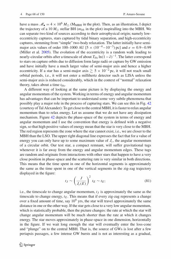
4 Page 68 of 150 P. Amaro-Seoane
have a mass M• = 4 × 10⁶ M� (MMBH in the plot). Then, as an illustration, I depictthe trajectory of a 10 M� stellar BH (mbh in the plot) inspiralling into the MBH. Wecan separate two kind of sources according to their astrophysical origin; namely low-eccentricity captures, stars captured by tidal binary separation, and high-eccentricitycaptures, stemming from “simple” two-body relaxation. The latter initially have semi-major axis values of order 100–1000 AU [5 × (10−4−10−3) pc] and e = 0.9−0.99(Miller et al. 2005). The evolution of the eccentricity is a random walk leading tonearly-circular orbits after a timescale of about Trlx ln(1− e)−1. The latter correspondto stars on capture orbits due to diffusion form large radii or capture by GW emissionand have initially have a much larger value of semi-major axis and hence a highereccentricity. If a star has a semi-major axis � 5 × 10⁻² pc, it will not reach smallorbital periods, i.e., it will not enter a millihertz detector such as LISA unless thesemi-major axis is reduced considerably, which in the context of “normal” relaxationtheory, takes about a time trlx.
A different way of looking at the same picture is by displaying the energy andangular momentum of the system. Working in terms of energy and angular momentumhas advantages that can be important to understand some very subtle phenomena thatpossibly play a major role in the process of capturing stars. We can see this in Fig. 42(courtesy of Tal Alexander): To get close to the central MBH, it is faster to relax angularmomentum than to relax energy. Let us assume that we do not have any dissipationmechanism. Figure 42 depicts the phase-space of the system in terms of energy andangular momentum and I use the convention that energy is defined with a negativesign, so that high positive values of energy mean that the star is very close to the MBH.The red region represents the zone where the star cannot exist, i.e., we are closer to theMBH than the LSO. The upper right diagonal line expresses the fact that for a value ofenergy you can only have up to some maximum value of Jc, the angular momentumof a circular orbit. Our test star, a compact remnant, will suffer gravitational tugswhenever it is far away from the energy and angular momentum edges. These tugsare random and originate from interactions with other stars that happen to have a veryclose position in phase-space and the scattering rate is very similar in both directions.This means that the time spent in one of the horizontal segments is approximatelythe same as the time spent in one of the vertical segments in the zig-zag trajectorydisplayed in the figure:
tJ ∼(
J
Jc(E)
)2
tE ∼ tE ; (81)
i.e., the timescale to change angular momentum, tJ is approximately the same as thetimescale to change energy, tE . This means that if every zig-zag represents a changeover a fixed amount of time, say 109 yrs, the star will travel approximately the samedistance in one or the other way. If the star gets close to a very low angular momentum,which is statistically probable, then the picture changes: the rate at which the star willchange angular momentum will be much shorter than the rate at which it changesenergy. The star moves approximately in phase-space in one dimension, horizontallyin the figure. If we wait long enough the star will eventually enter the loss-coneand “plunge” on to the central MBH. That is, the source of GWs is lost after a fewperiapsis passages, a few intense GW bursts and is not as interesting as a gradual,
123

Relativistic dynamics and extreme mass ratio inspirals Page 69 of 150 4
J = J (E)c
lscolog E
log Jlc log J
short P
long P
log E
"Spherical background"
1D J−scattering
Plunge
lc
log E
log J
Inspiral
Plunge
NR
RR
log J
critlog E
lscolog E
cJ = J (E)
Transitionphase
E−dissipationphase Detectable GW
J−scattering phase
Fig. 42 Plunge, inspiral and critical energy of an EMRI in phase-space. Left panel: Direct plunge of asource. Right panel: Adiabatic inspiral of a source subject to dissipation of energy at periapsis and limitingcritical energy (image courtesy of Tal Alexander)
slowly inspiraling source. This picture corresponds to the general scenario that wasdescribed already a few decades ago, when people were investigating ways of feedingthe MBH (Lightman and Shapiro 1977; Cohn and Kulsrud 1978).
However, if we have a dissipation process acting on to the star, which could beenergy loss in the form of GWs as well as drag forces originating in an accretion discor, obviously tidal forces created by the central MBH, the picture changes significantly.The process follows the same path and, at some point, the star reaches the region inwhich it is on a very radial orbit, i.e. where the zig-zag stops and we can approximatethe curve by a horizontal line. Nonetheless, in this case, at every periapsis passage,the star will emit an intense burst of GWs and, thus, shrink its semi-major axis. Ifthis happens “efficiently enough”, i.e., “fast enough” (we will elaborate on this later),the star is more and more bound to the central MBH and drifts away (goes up in theenergy axis of the figure). The danger of being scattered away from the capture orbitby other stars decreases more and more and the compact object finds itself on a safeinspiraling EMRI orbit. The precise details of the dynamics that lead to this situationdetermines the distribution of eccentricities that we can expect. The semi-major axisshrinks to the point that the source enters the “Detectable GW” regime (light-blueband in the right panel of Fig. 42). As the source advances in that band, the periodbecomes shorter and shorter and, hence, the power (emitted energy per unit of time)grows larger and larger, so that the gravitational radiation can be measured when itenters the frequency band of the observatory.
The statistical orbital properties of the EMRI in the region where GW emission isprominent are fully determined by the transition phase between the region dominatedby 2-body scattering processes (the right part of the curve) of the random walk inphase-space and the deterministic dissipation part of the capture trajectory, i.e., wherethe energy loss occurs.
As described in Hopman and Alexander (2005), in this statistical treatment thereis a critical energy, i.e., a certain distance from the central MBH, of the order ∼ 10−2
pc, that can be envisaged as the threshold between the two regions. This means thatstars with energy below the yellow dashed line of the right panel of Fig. 42 will have
123

4 Page 70 of 150 P. Amaro-Seoane
Standard relaxationalprocess
Tidal separation
Fig. 43 Capture trajectories in the a – (1 − e) plane and tidal disruption limit. See text for a detailedexplanation of the figure
“longer horizontal segments”, they will scatter faster in angular momentum than inenergy and then they will end up as direct plunges. They approach the central MBH insuch a radial orbit that they are swallowed after one or, at most, a few intense bursts ofGWs. This situation is reverted if the energy of the star is above the line; the star willspiral in adiabatically and it will not be perturbed out of the EMRI trajectory, with asignificant amount of GW bursts at periapsis before coalescing with the MBH.
Hence, and again, statistically at first order, one has to consider only stars whoseenergy falls within the critical region and we can ignore all other stars, even if theirenergy and angular momentum indicate that they are good candidates for EMRIs.Thus, the event rate will be determined by the “microphysics” affecting the innermostvolume around the MBH, of radius ∼ 10−2 pc. As the reader will surely have guessedby now, the task is non-trivial.
7 Beyond the standard model of two-body relaxation
7.1 The standard picture
The intelligent reader will very surely have realised that the picture is much morecomplex than plain two-body relaxation. Quoting something that Sterling Colgatesaid once in Aspen,
123

Relativistic dynamics and extreme mass ratio inspirals Page 71 of 150 4
Do you know what the standard (American) model is? : One gallon per flush.
Although Sterling was not directly referring to our standard model, of course. Thismeans that, illustrating and enlightening as it might be, the standard model we havebeen describing so far must be regarded as a (probably very well) educated guess.
As the interest in a millihertz mission started to grow and develop, astrophysicistsstarted to dedicate more and more time to a problem that, naively, was not very difficult.How do you get a small black hole into a massive black hole in a galactic nucleus? Now,some decades after the very first estimates, we have a much better and clear vision ofthe main phenomena at play in the process. Well before any space-borne mission islaunched, our understanding of theory related to stellar dynamics has become muchbroader and new, unexpected effects have emerged.
7.2 Coherent or resonant relaxation14
As I have discussed previously, in a gravitational potential with a high degree ofsymmetry, a test star will receive gravitational tugs from the rest of the field starswhich are not totally arbitrary and hence do not add up in a random walk way, butcoherently. As we have seen in Sect. 3, the potential will prevent stellar orbits fromevolving in an erratic way. In a two-body Keplerian system, a SBH will orbit aroundthe MBH in a fixed ellipse. The stellar BH will not feel random gravitational tugs. Itevolves coherently as the result of the action of the gravitational potential. When anEMRI approaches the periapsis of its orbit, we can envisage the situation as a puretwo-body problem; initially Newtonian but later GR effects must be taken into accountas the periapsis grows smaller and smaller. Nonetheless, as the stellar BH goes backto the apoapsis, it will feel the surrounding stellar system, distributed in the shapeof a cusp which grows in mass the further away we are from the periapsis. The timespent in the region in which we can regard this as a two-body problem is much shorterthan the time in which the stellar BH will feel the rest of the stellar system. This isparticularly true for the kind of objects of our interest, since the very high eccentricityimplies a large semi-major axis. The time spent on periapsis is negligible as comparedwith the time spent on apoapsis, so that the stellar BH can feel the graininess of thepotential. The gravitational tugs from other stars will alter its orbit. The mean free pathin angular momentum-space of that test stellar BH is very large and thus, it has a fastrandom walk. Both the magnitude and direction of angular momentum of the stellarblack hole are altered. When the magnitude changes but not the direction, we talk of“scalar” resonant relaxation, and correspondingly when the direction is changed butnot the size, “vector” resonant relaxation.
A very radial orbit can become a very eccentric one, so that a compact objectinitially set on a potential EMRI orbit can be “pushed out” of it. In a more generalcase, a spherical potential that is non-Keplerian, the orbits, as we have describedbefore, are rosettes and averaged over time they are circular anuli. In that case we can
14 The reason for the title of this section is that probably the choice of “resonant” for this process is not agood one. Rauch and Tremaine (1996) coined this term thinking of the effect of a resonance between theradial and azimuthal periods in a Keplerian orbit.
123

4 Page 72 of 150 P. Amaro-Seoane
Fig. 44 If we have a point-likepotential, scalar coherentrelaxation can modify the size ofangular momentum and theinclination of the orbital plane ofa test star. Dashed lines depictthe perturbing orbits on the teststar, m•, whose orbit isdisplayed as a solid line in twomoments of the evolution
m•
M•
M•m•
change the direction of angular momentum but not the modulus. An eccentric orbitwill stay eccentric, but any coherence that was there will be washed out.
In particular, as illustrated in Fig. 44, in the potential of a point mass, orbits arefrozen fixed ellipses that exert a continuous torque on the test star. A test star does notfeel random kicks from all directions. When we add up the individual contributionscoming from all the rest of stars on to the test star, there is a residual, non-negligibletorque that will influence its evolution. The mean free path of the star in angularmomentum space is very large. I will refer to this phenomenon as scalar coherentrelaxation, because it can change both the magnitude of angular momentum and theinclination of the orbital plane of the test star. This scenario is a possible way to alteran initially very circular orbit and modify it in such a way that the test star will getvery close to the MBH after the torques have acted. That is, we open a new windowfor stars to fall into a capture orbit that will lead to an EMRI.
In a more general case, if we have a potential that is simply spherical but notnecessarily Keplerian (a point mass), the field stars, the perturbing orbits to the test star,describe rosettes -as we have seen- and averaged over time they can be approximatedby a set of anuli that share a centre. From a secular point of view, the masses aresmeared over those anuli which create torques that do not change the magnitude ofangular momentum but they do change the orientation because of reasons of symmetry(Rauch and Tremaine 1996; Rauch and Ingalls 1998; Hopman and Alexander 2006b).Hence a circular test star will keep a negligible eccentricity and it will not approachthe central MBH. Any coherence that was present in the system will nonetheless bedestroyed. I will refer to this as vectorial coherent relaxation. From the standpoint ofEMRI production, though, this process is not as relevant and we will not elaborate onit further, though it can be very relevant for phenomena related to galactic nuclei, forinstance, warping of accretion discs (Bregman and Alexander 2009).
However, one must note that these illustrations are oversimplifications and depictperfect symmetries that might be affected or even totally cancelled out by other effectssuch as, e.g., the relativistic periapsis shift or Newtonian precession. Thus, after acertain time this symmetry is broken and the evolution is again a random walk, onewith very large stepsize. I refer the reader to the review of Alexander (2007) for adetailed and excellent description of these processes.
123
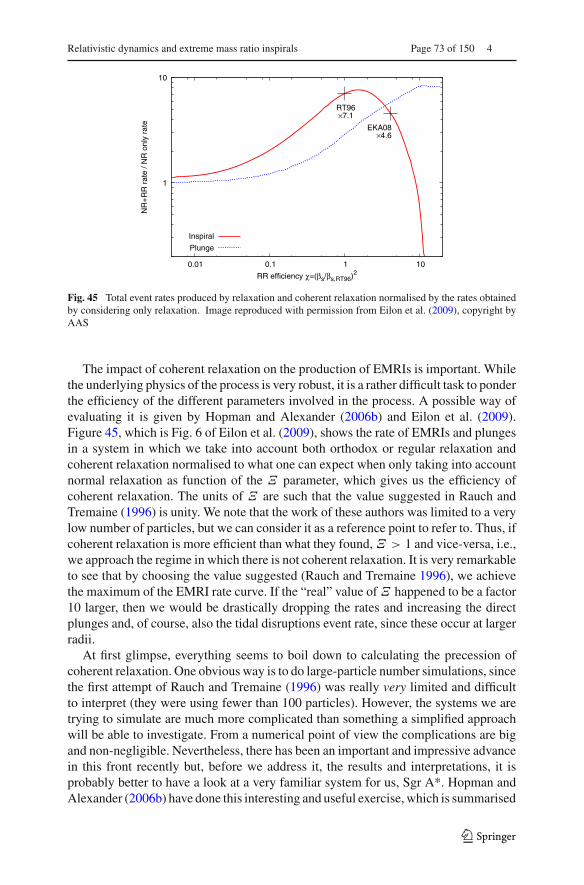
Relativistic dynamics and extreme mass ratio inspirals Page 73 of 150 4
1
10
0.01 0.1 1 10
NR
+R
R r
ate
/ NR
onl
y ra
te
RR efficiency χ=(βs/βs,RT96)2
Inspiral
Plunge
RT96×7.1
EKA08×4.6
Fig. 45 Total event rates produced by relaxation and coherent relaxation normalised by the rates obtainedby considering only relaxation. Image reproduced with permission from Eilon et al. (2009), copyright byAAS
The impact of coherent relaxation on the production of EMRIs is important. Whilethe underlying physics of the process is very robust, it is a rather difficult task to ponderthe efficiency of the different parameters involved in the process. A possible way ofevaluating it is given by Hopman and Alexander (2006b) and Eilon et al. (2009).Figure 45, which is Fig. 6 of Eilon et al. (2009), shows the rate of EMRIs and plungesin a system in which we take into account both orthodox or regular relaxation andcoherent relaxation normalised to what one can expect when only taking into accountnormal relaxation as function of the Ξ parameter, which gives us the efficiency ofcoherent relaxation. The units of Ξ are such that the value suggested in Rauch andTremaine (1996) is unity. We note that the work of these authors was limited to a verylow number of particles, but we can consider it as a reference point to refer to. Thus, ifcoherent relaxation is more efficient than what they found, Ξ > 1 and vice-versa, i.e.,we approach the regime in which there is not coherent relaxation. It is very remarkableto see that by choosing the value suggested (Rauch and Tremaine 1996), we achievethe maximum of the EMRI rate curve. If the “real” value of Ξ happened to be a factor10 larger, then we would be drastically dropping the rates and increasing the directplunges and, of course, also the tidal disruptions event rate, since these occur at largerradii.
At first glimpse, everything seems to boil down to calculating the precession ofcoherent relaxation. One obvious way is to do large-particle number simulations, sincethe first attempt of Rauch and Tremaine (1996) was really very limited and difficultto interpret (they were using fewer than 100 particles). However, the systems we aretrying to simulate are much more complicated than something a simplified approachwill be able to investigate. From a numerical point of view the complications are bigand non-negligible. Nevertheless, there has been an important and impressive advancein this front recently but, before we address it, the results and interpretations, it isprobably better to have a look at a very familiar system for us, Sgr A*. Hopman andAlexander (2006b) have done this interesting and useful exercise, which is summarised
123

4 Page 74 of 150 P. Amaro-Seoane
Fig. 46 The different timescalesdominating stellar dynamics inthe Galactic Centre. Imagereproduced with permissionfrom Hopman and Alexander(2006b), copyright by AAS
10−3 10−2 10−1 1a (pc)
101
102
103
104
t (M
yr)
TNR
T_ s
RR TvRR
Star disks
S- stars
GW sources
Relaxed giants
in their Fig. 6 (see Fig. 46). In this figure, the authors display the relevance of differentdynamical components in an attempt to constrain the strength of coherent relaxation.
On the vertical axes, we have the age of different systems found in the GC asfunction of the semi-major axis of the stars with the object in Sgr A*. On the top of thefigure we see a line giving us the timescale for normal relaxation, TNR to use the samenomenclature as the authors and their plot, which is shorter than the Hubble time butnot much shorter. The following two curves from the top give the timescale for scalarcoherent relaxation for two cases, the first curve from the top corresponds to a systemof 1 M� stars and 10 M� stars at large values the effect is quenched by the presence ofan extended mass, i.e., Newtonian precession and at short distances it is periapsis shiftthat decreases its strength. The minima displayed in the figure fence in the potentialrange of values for the efficiency. The “real” value probably lies somewhere in themiddle.
It is, nevertheless, important to note that the authors did not take into accountthe effect of a mass spectrum. In this respect, while it is easier to understand thefundamentals of the scenario, the system lacks an important ingredient in realism thatcould significantly change the narrative.
On the lower right corner of the figure, we have vector coherent relaxation, whichis much more efficient with associated timescales shorter than a million years for ashort enough semi-major axis.
In the same figure, we display the area from which we believe that EMRIs originate;i.e., within ∼ 0.01 pc. These objects are typically compact remnants and, hence, willbe accumulated in the top left corner of the figure because they are older than the typicaltime for relaxation. As we can see, and as shown in the calculations of the authors, theyare embedded in the area which is totally dominated by coherent relaxation. This is avery striking result from the standpoint of standard relaxation theory: The dynamics ofEMRIs will be dominated by this new “exotic” form of relaxation, coherent relaxationand not by normal (two-body) relaxation.
As I have already explained previously, there are different populations of stars inthe GC that we can observe. One of these is the disc stars, some ∼ 50–100 verymassive and young stars observed to be orbiting on discs and almost circularly. Theupper limit on the edge is of a few 106 M� and, thus, the strip in the figure is verynarrow. These discs are characterised by having a relatively well-defined and sharp
123

Relativistic dynamics and extreme mass ratio inspirals Page 75 of 150 4
inner cut-off. It is remarkable to note that the cut-off happens to be exactly at the placein the figure where the timescale associated with vectorial coherent relaxation (TV
RRin the plot) crosses the strip, without a fit, as Hopman and Alexander (2006b) claim.On the left side of the line, we have the S-stars, which are not on circular orbits, noraligned with the disc, but randomly orientated. They are sometimes envisaged as thelow-mass members of the disc of stars. In any case, it is intriguing that these stars lieexactly on the left of the curve, where we expect any disc structure to be destroyed byvectorial coherent relaxation. This would imply that the values derived by Rauch andTremaine (1996) are very close to the real ones. While it is probably too early to makeany strong statement from this fact, it is encouraging enough to keep us studying andtrying to understand normal as well as coherent relaxation in galactic nuclei. Anotherinterpretation of Fig. 46 is that we can expect some of the S-stars to have randomeccentricities due to the fact that those which are close enough are affected by scalarcoherent relaxation. Also, we can in principle explain why late-type giants do not haveany particular orientation in their orbits, since they are in that part of the plot.
The numerical simulations of Eilon et al. (2009) show that coherent relaxation canenhance the EMRI rate by a factor of a few over the rates predicted assuming onlyslow stochastic two-body relaxation, as the authors prove.
7.3 Strong mass segregation
We have seen in Sect. 5 that stars with different mass get distributed around a MBH ina galactic nucleus with different density profile. We devoted a significant part of thatsection to studying the case of single-mass, which was described in an analytical wayby Bahcall and Wolf (1976), and previously in Peebles (1972). The authors extendedthe work to stellar systems with two mass components and argued heuristically for ascaling relation that depends on the star’s mass ratio only, namely pL = mL/mH × pH(Bahcall and Wolf 1977). They did not give a general result on inner slope of theheavy stars (the stellar-mass black holes in our case) and they did not discuss thedependence of the result on the component’s number fractions. Fortunately, Alexanderand Hopman (2009) addressed this issue and found that there exist two branches ofsolutions, parametrised by
Δ ≈ NHm2H
NLm2L
4
3 + mH/mL, (82)
where capital letters denote total stellar mass and lower-case letters individual massesof stars. The quantity Δ gives us a measure of the relevance of the SBH self-couplingrelative to the other species coupling, the lighter stars in the system, and the mainadvantage of it is that it depends basically on the mass and number ratios. In thisrespect, Alexander and Hopman (2009) extend the study of Bahcall and Wolf (1977) toan additional, crucial parameter. For values of Δ > 1 we recover the scaling solutionsof Bahcall and Wolf (1977). This is the regime that Alexander and Hopman (2009)refer to as the “weak branch” of the solution. On the other hand, for Δ < 1, we havea new kind of solution that generalises the solution of Bahcall and Wolf (1977). This
123
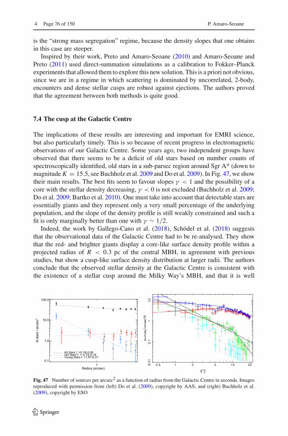
4 Page 76 of 150 P. Amaro-Seoane
is the “strong mass segregation” regime, because the density slopes that one obtainsin this case are steeper.
Inspired by their work, Preto and Amaro-Seoane (2010) and Amaro-Seoane andPreto (2011) used direct-summation simulations as a calibration to Fokker–Planckexperiments that allowed them to explore this new solution. This is a priori not obvious,since we are in a regime in which scattering is dominated by uncorrelated, 2-body,encounters and dense stellar cusps are robust against ejections. The authors provedthat the agreement between both methods is quite good.
7.4 The cusp at the Galactic Centre
The implications of these results are interesting and important for EMRI science,but also particularly timely. This is so because of recent progress in electromagneticobservations of our Galactic Centre. Some years ago, two independent groups haveobserved that there seems to be a deficit of old stars based on number counts ofspectroscopically identified, old stars in a sub-parsec region around Sgr A* (down tomagnitude K = 15.5, see Buchholz et al. 2009 and Do et al. 2009). In Fig. 47, we showtheir main results. The best fits seem to favour slopes γ < 1 and the possibility of acore with the stellar density decreasing, γ < 0 is not excluded (Buchholz et al. 2009;Do et al. 2009; Bartko et al. 2010). One must take into account that detectable stars areessentially giants and they represent only a very small percentage of the underlyingpopulation, and the slope of the density profile is still weakly constrained and such afit is only marginally better than one with γ ∼ 1/2.
Indeed, the work by Gallego-Cano et al. (2018), Schödel et al. (2018) suggeststhat the observational data of the Galactic Centre had to be re-analysed. They showthat the red- and brighter giants display a core-like surface density profile within aprojected radius of R < 0.3 pc of the central MBH, in agreement with previousstudies, but show a cusp-like surface density distribution at larger radii. The authorsconclude that the observed stellar density at the Galactic Centre is consistent withthe existence of a stellar cusp around the Milky Way’s MBH, and that it is well
1Radius (arcsec)
0.1
1.0
10.0
100.0
N s
tars
/ ar
csec
2
Young Stars Γ =1.51±0.21Old Stars Γ =−0.12±0.16All Stars Γ =0.19±0.06
Fig. 47 Number of sources per arcsec2 as a function of radius from the Galactic Centre in seconds. Imagesreproduced with permission from (left) Do et al. (2009), copyright by AAS; and (right) Buchholz et al.(2009), copyright by ESO
123
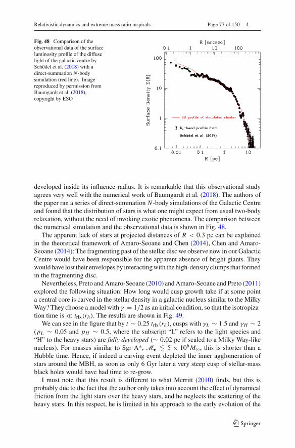
Relativistic dynamics and extreme mass ratio inspirals Page 77 of 150 4
Fig. 48 Comparison of theobservational data of the surfaceluminosity profile of the diffuselight of the galactic centre bySchödel et al. (2018) with adirect-summation N -bodysimulation (red line). Imagereproduced by permission fromBaumgardt et al. (2018),copyright by ESO
developed inside its influence radius. It is remarkable that this observational studyagrees very well with the numerical work of Baumgardt et al. (2018). The authors ofthe paper ran a series of direct-summation N -body simulations of the Galactic Centreand found that the distribution of stars is what one might expect from usual two-bodyrelaxation, without the need of invoking exotic phenomena. The comparison betweenthe numerical simulation and the observational data is shown in Fig. 48.
The apparent lack of stars at projected distances of R < 0.3 pc can be explainedin the theoretical framework of Amaro-Seoane and Chen (2014), Chen and Amaro-Seoane (2014): The fragmenting past of the stellar disc we observe now in our GalacticCentre would have been responsible for the apparent absence of bright giants. Theywould have lost their envelopes by interacting with the high-density clumps that formedin the fragmenting disc.
Nevertheless, Preto and Amaro-Seoane (2010) and Amaro-Seoane and Preto (2011)explored the following situation: How long would cusp growth take if at some pointa central core is carved in the stellar density in a galactic nucleus similar to the MilkyWay? They choose a model with γ = 1/2 as an initial condition, so that the isotropiza-tion time is � trlx(rh). The results are shown in Fig. 49.
We can see in the figure that by t ∼ 0.25 trlx(rh), cusps with γL ∼ 1.5 and γH ∼ 2(pL ∼ 0.05 and pH ∼ 0.5, where the subscript “L” refers to the light species and“H” to the heavy stars) are fully developed (∼ 0.02 pc if scaled to a Milky Way-likenucleus). For masses similar to Sgr A*, M• � 5 × 10⁶M�, this is shorter than aHubble time. Hence, if indeed a carving event depleted the inner agglomeration ofstars around the MBH, as soon as only 6 Gyr later a very steep cusp of stellar-massblack holes would have had time to re-grow.
I must note that this result is different to what Merritt (2010) finds, but this isprobably due to the fact that the author only takes into account the effect of dynamicalfriction from the light stars over the heavy stars, and he neglects the scattering of theheavy stars. In this respect, he is limited in his approach to the early evolution of the
123
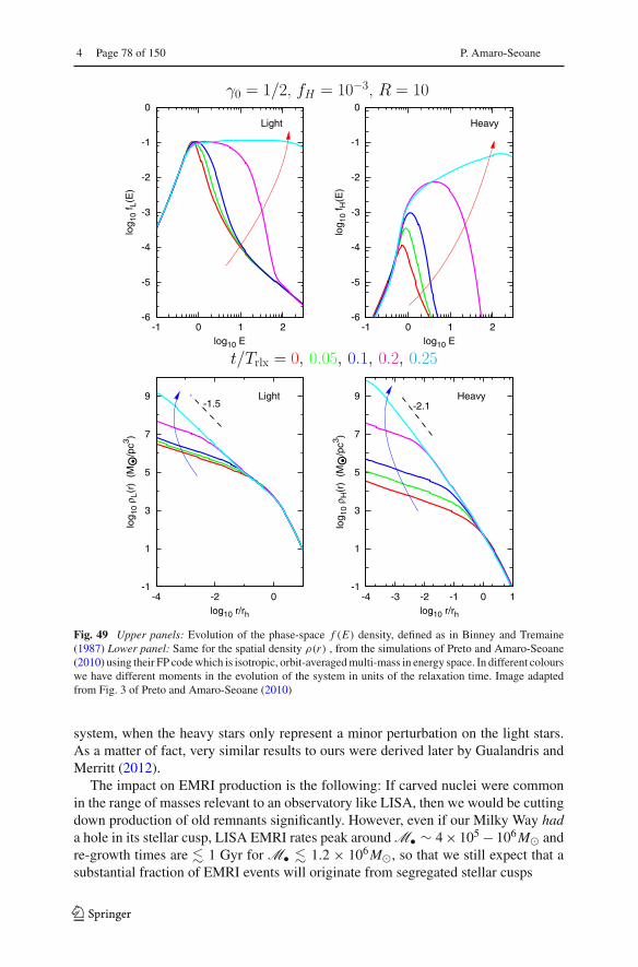
4 Page 78 of 150 P. Amaro-Seoane
-6
-5
-4
-3
-2
-1
0
-1 0 1 2
log 1
0 f L
(E)
log10 E
Light
-6
-5
-4
-3
-2
-1
0
-1 0 1 2lo
g 10
f H(E
)log10 E
Heavy
-1
1
3
5
7
9
-4 -2 0
log 1
0 ρ L
(r)
(M
O• /p
c3 )
log10 r/rh
Light-1.5
-1
1
3
5
7
9
-4 -3 -2 -1 0 1
log 1
0 ρ H
(r)
(M
O• /p
c3 )
log10 r/rh
-2.1Heavy
t/Trlx = 0, 0.05, 0.1, 0.2, 0.25
γ0 = 1/2, fH = 10−3, R = 10
Fig. 49 Upper panels: Evolution of the phase-space f (E) density, defined as in Binney and Tremaine(1987) Lower panel: Same for the spatial density ρ(r) , from the simulations of Preto and Amaro-Seoane(2010) using their FP code which is isotropic, orbit-averaged multi-mass in energy space. In different colourswe have different moments in the evolution of the system in units of the relaxation time. Image adaptedfrom Fig. 3 of Preto and Amaro-Seoane (2010)
system, when the heavy stars only represent a minor perturbation on the light stars.As a matter of fact, very similar results to ours were derived later by Gualandris andMerritt (2012).
The impact on EMRI production is the following: If carved nuclei were commonin the range of masses relevant to an observatory like LISA, then we would be cuttingdown production of old remnants significantly. However, even if our Milky Way hada hole in its stellar cusp, LISA EMRI rates peak around M• ∼ 4 × 10⁵ − 106M� andre-growth times are � 1 Gyr for M• � 1.2 × 10⁶M�, so that we still expect that asubstantial fraction of EMRI events will originate from segregated stellar cusps
123
Relativistic dynamics and extreme mass ratio inspirals Page 79 of 150 4
On the other hand, strong mass segregation not only “comes to the rescue” in thecase of carved nuclei. It helps in the production of EMRIs. Amaro-Seoane and Preto(2011) estimate that thanks to strong mass segregation one might expect EMRI evenrates to be ∼ 1 − 2 orders of magnitude larger than one would expect from using theBahcall and Wolf solution, as they show.
Their solution for the weak branch is physically unrealistic, since it predicts a toohigh event rate because it uses unreasonably high number fractions of stellar-massblack holes f• (≥ 0.05). In a more realistic case, when Δ ∼ 0.03, ( f• ∼ 10−3) theBahcall and Wolf solution would lead to a strong suppression of the EMRI rate to—atbest—a few tens of events per Gyr.
The new solution of strong mass segregation implies a higher ρ• well inside theinfluence radius of the MBH, so that we have a boost in the diffusion of stellar-massblack holes close to the MBH. When going from number fractions that are based onunrealistic IMF, such as in Bahcall and Wolf (1977) (say Δ = 3) to realistic values(Δ = 0.03), the event rate is suppressed by factors of ∼ 100–150, if we ignore strongmass segregation. Thanks to this new solution, based on more realistic physics, evenfor low values of Δ = 0.03, we boost the rates from few tens to a few hundred perGyr, ∼ 250/Gyr if we consider a mass ratio of 10 between the stellar-mass black holesand the MS stars and if we take a fractional number for stellar-mass black holes off• = 0.001.
7.5 Tidal separation of binaries
Another process contributing to the creation of EMRIs has its origin in the work of Hills(1988), where he describes the possibility of finding escaping stars that originate bythis process:
A close but Newtonian encounter between a tightly bound binary and a millionsolar mass black hole causes one binary component to become bound to theblack hole and the other to be ejected at up to 4000 km/s. The discovery of evenone such hypervelocity star coming from the Galactic center would be nearlydefinitive evidence for a massive black hole. The new companion of the blackhole has a high orbital velocity which increases further as its orbit shrinks bytidal dissipation. The gravitational energy released by the orbital shrinkage ofsuch a tidal star can be comparable to its total nuclear energy release.
His work, about the tidal separation of binaries by a MBH, did not have a bigimpact for some 15 years until the discovery of the so-called “hyper-velocity stars”,stars with a velocity of > 103 km s−1, which he had predicted. Indeed, several suchstars have been discovered in the last years. I refer the reader to Brown et al. (2009)for a discussion of the properties of these stars, as well as for references.
While one of the objects is ejected into the stellar system, the other binary membercan remain bound to the MBH on a rather tight orbit. If this star happens to be acompact object, then we would have an EMRI which would be rather “immune” tothe problems of EMRIs caused by two-body relaxation. Since the tidal separationhappens very close to the MBH, the CO will have a shorter apoapsis (usually only tens
123

4 Page 80 of 150 P. Amaro-Seoane
Fig. 50 Schematic illustrationof the process of the tidalseparation of a binary by a MBHof mass M•. Rsplit is defined asthe radius within which the tidalforces of the MBH overcome thebinding energy of the binary Rsplit
M•acapt
Captured star (m•)
High-velocity star
v
Binary star a
of times the periapsis distance) and thus, potential tugs that lead it out of the captureorbit are reduced. This process was described by Miller et al. (2005). The propertiesof these EMRIs are very interesting and I describe the process in this section, bothfrom an astrophysical point of view and the observational signature.
In Fig. 50, we have a schematic view of the process. A binary which happens to flyby close enough to the central MBH will be tidally separated because the tides actingon the pair overcome the gravity in the binary. One of the stars is captured, meaningthat it will be bound to the MBH, after losing a little energy compared to what it hadbefore, and the other companion of the binary will obtain a bit more energy after theseparation, so that it will be ejected with a high velocity, as in a slingshot. It is ratherstraightforward to make a toy model for the process and get the scalings, which shedslight on the process.
The size of the region where this process will occur, Rsplit , is proportional to thesize of the object, the separation of the binary (i.e. about the semi-major axis), themass of the binary mbin and the mass of the central MBH, M•, as it was in the caseof the tidal disruption of an extended star. Actually, we can follow the analogy veryclosely, except in that case we have to come closer to the MBH to have the tidal forcesovercoming the binding energy of the binary, since a > R�, with R� the radius of thestar.
Rsplit ∼ a
(M•mbin
)1/3
. (83)
The orbital velocity in the binary can be easily computed as follows,
v ∼√G mbin
a. (84)
123

Relativistic dynamics and extreme mass ratio inspirals Page 81 of 150 4
Fig. 51 Zoom of Fig. 50 for thesplitting of the pair. I assume aparabolic encounter (dashedcurve) for the COM of thebinary and a mass m• and m�
for the stars
m• m�
VCM + v
M•
Captured companionVCM − v
High-velocity star
I now normalise the last equation to nominal values assuming that it is a hard binaryin a galactic nucleus,
v ∼ 133 km s−1(mbin
2M�
)1/2 ( a
0.1AU
)−1/2. (85)
Figure 51 shows a zoom-in of Fig. 50 at the moment in which the binary is atthe periapsis of the MBH. We now estimate the ejection velocity. The centre-of-mass(CM) of the binary has a velocity VCM which we can easily calculate by assuming thatthe encounter is parabolic
VCM �√GM•Rsplit
∼ v
(M•mbin
)1/3
� v. (86)
This allows us to estimate the ejection velocity of the slingshot star, because thedifference of energy will be
± δE � VCM · v ≥ v2(M•mbin
)1/3
� v2eject
2. (87)
Then, we have that
veject �(M•mbin
)1/6
. (88)
Since we are dealing with a binary, the star of mass m•, which we assume to be astellar-mass black hole, will be slowed down by v, as in Eq. (84) and the star of mass
123
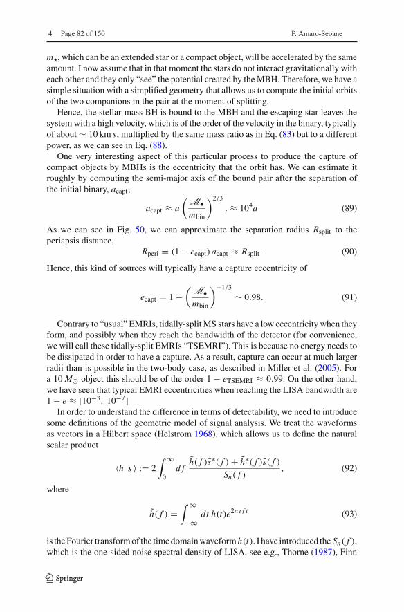
4 Page 82 of 150 P. Amaro-Seoane
m�, which can be an extended star or a compact object, will be accelerated by the sameamount. I now assume that in that moment the stars do not interact gravitationally witheach other and they only “see” the potential created by the MBH. Therefore, we have asimple situation with a simplified geometry that allows us to compute the initial orbitsof the two companions in the pair at the moment of splitting.
Hence, the stellar-mass BH is bound to the MBH and the escaping star leaves thesystem with a high velocity, which is of the order of the velocity in the binary, typicallyof about ∼ 10 km s, multiplied by the same mass ratio as in Eq. (83) but to a differentpower, as we can see in Eq. (88).
One very interesting aspect of this particular process to produce the capture ofcompact objects by MBHs is the eccentricity that the orbit has. We can estimate itroughly by computing the semi-major axis of the bound pair after the separation ofthe initial binary, acapt,
acapt ≈ a
(M•mbin
)2/3
. ≈ 104a (89)
As we can see in Fig. 50, we can approximate the separation radius Rsplit to theperiapsis distance,
Rperi = (1 − ecapt) acapt ≈ Rsplit. (90)
Hence, this kind of sources will typically have a capture eccentricity of
ecapt = 1 −(M•mbin
)−1/3
∼ 0.98. (91)
Contrary to “usual” EMRIs, tidally-split MS stars have a low eccentricity when theyform, and possibly when they reach the bandwidth of the detector (for convenience,we will call these tidally-split EMRIs “TSEMRI”). This is because no energy needs tobe dissipated in order to have a capture. As a result, capture can occur at much largerradii than is possible in the two-body case, as described in Miller et al. (2005). Fora 10 M� object this should be of the order 1 − eTSEMRI ≈ 0.99. On the other hand,we have seen that typical EMRI eccentricities when reaching the LISA bandwidth are1 − e ≈ [10−3, 10−7]
In order to understand the difference in terms of detectability, we need to introducesome definitions of the geometric model of signal analysis. We treat the waveformsas vectors in a Hilbert space (Helstrom 1968), which allows us to define the naturalscalar product
〈h |s 〉 := 2∫ ∞
0d f
h( f )s∗( f ) + h∗( f )s( f )Sn( f )
, (92)
where
h( f ) =∫ ∞
−∞dt h(t)e2π ı f t (93)
is the Fourier transform of the time domain waveformh(t). I have introduced the Sn( f ),which is the one-sided noise spectral density of LISA, see e.g., Thorne (1987), Finn
123

Relativistic dynamics and extreme mass ratio inspirals Page 83 of 150 4
Fig. 52 Waveforms of a normal EMRI and a TSEMRI (see text) superimposed for a full year of data beforethe final plunge, which has been defined to happen at a periapsis of rplunge ≡ 2 × rISCO, with rISCO theradius of the innermost stable circular orbit, which is ∼ 8 M in this case. The mass of the central MBH is3 × 106 M�, the mass of the star 0.53 M�. The spin of the MBH is set to a = 0.5 M and we neglect thespin of the star
(1992). One can think of LISA as two detectors, so that the signal in each of themis given by si (t) = hi (t) + ni (t), with i = 1, 2 label each detector. I adopt theassumption that the noise ni (t) is stationary, Gaussian, uncorrelated in each detectorand characterised by the noise spectral density Sn( f ). Hence, we can define the signal-to-noise ratio in each detector as
ρi = 〈h |si 〉√〈h |h 〉 . (94)
Therefore, if we consider the waveform of a TSEMRI and compare it with a normalEMRI, we can calculate the mismatch of their expected signal-to-noise ratio for LISAas
M := 1 − 〈hTSEMRI |hEMRI 〉√〈hTSEMRI |hTSEMRI 〉 〈hEMRI |hEMRI 〉 . (95)
For a TSEMRI and a normal EMRI starting with exactly the same orbital parametersat the GC and coloured for LISA, I have calculated with the LISACode15 (Petiteauet al. 2008) that there is a mismatch of 99.9971%. Using the standard definition ofsignal-to-noise ratio ρi = 〈h|si 〉 /
√〈h|h〉, we have that the TSEMRI is calculated tohave an average signal-to-noise ratio of ρTSMI ∼ 27637 and the normal EMRI ofρEMRI ∼ 18848, both set to be at a distance of 8.3 kpc.
Figure 52 shows the waveforms for an observer at θ = 55 degrees, with originat the MBH, with a mass of 3 · 106 M� and z-axis along direction of big black holespin. The waveforms are from Steve Drasco and have been calculated using the kludgeapproximation of Gair and Glampedakis (2006) (Fig. 53).
15 http://www.apc.univ-paris7.fr/~petiteau/LISACode/Home.html.
123
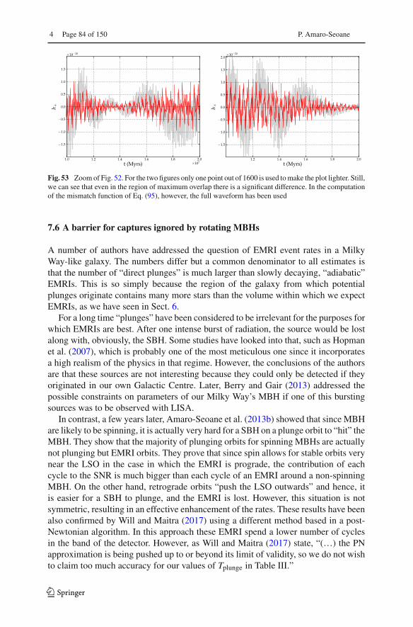
4 Page 84 of 150 P. Amaro-Seoane
Fig. 53 Zoom of Fig. 52. For the two figures only one point out of 1600 is used to make the plot lighter. Still,we can see that even in the region of maximum overlap there is a significant difference. In the computationof the mismatch function of Eq. (95), however, the full waveform has been used
7.6 A barrier for captures ignored by rotating MBHs
A number of authors have addressed the question of EMRI event rates in a MilkyWay-like galaxy. The numbers differ but a common denominator to all estimates isthat the number of “direct plunges” is much larger than slowly decaying, “adiabatic”EMRIs. This is so simply because the region of the galaxy from which potentialplunges originate contains many more stars than the volume within which we expectEMRIs, as we have seen in Sect. 6.
For a long time “plunges” have been considered to be irrelevant for the purposes forwhich EMRIs are best. After one intense burst of radiation, the source would be lostalong with, obviously, the SBH. Some studies have looked into that, such as Hopmanet al. (2007), which is probably one of the most meticulous one since it incorporatesa high realism of the physics in that regime. However, the conclusions of the authorsare that these sources are not interesting because they could only be detected if theyoriginated in our own Galactic Centre. Later, Berry and Gair (2013) addressed thepossible constraints on parameters of our Milky Way’s MBH if one of this burstingsources was to be observed with LISA.
In contrast, a few years later, Amaro-Seoane et al. (2013b) showed that since MBHare likely to be spinning, it is actually very hard for a SBH on a plunge orbit to “hit” theMBH. They show that the majority of plunging orbits for spinning MBHs are actuallynot plunging but EMRI orbits. They prove that since spin allows for stable orbits verynear the LSO in the case in which the EMRI is prograde, the contribution of eachcycle to the SNR is much bigger than each cycle of an EMRI around a non-spinningMBH. On the other hand, retrograde orbits “push the LSO outwards” and hence, itis easier for a SBH to plunge, and the EMRI is lost. However, this situation is notsymmetric, resulting in an effective enhancement of the rates. These results have beenalso confirmed by Will and Maitra (2017) using a different method based in a post-Newtonian algorithm. In this approach these EMRI spend a lower number of cyclesin the band of the detector. However, as Will and Maitra (2017) state, “(…) the PNapproximation is being pushed up to or beyond its limit of validity, so we do not wishto claim too much accuracy for our values of Tplunge in Table III.”
123

Relativistic dynamics and extreme mass ratio inspirals Page 85 of 150 4
Fig. 54 The Schwarzschild barrier. In the left panel, we have the Newtonian case and in the right one thesimulations with relativistic corrections. We clearly see the barrier and also a particle crossing it. Imagesreproduced with permission from arXiv e-print of Merritt et al. (2011)
Amaro-Seoane et al. (2013b) also show that vectorial coherent relaxation is notefficient enough to turn a prograde orbit into a retrograde one, which would be fatalfor this scenario, once the evolution is dominated by GW emission. This result is crucialin the formation of EMRI sources. To understand why, first we need to introduce theproblem of the so-called “Schwarzschild barrier”.
Merritt et al. (2011) performed direct-summation N -body simulations and foundthat EMRI event rates are severely suppressed when introducing relativistic precessionin the integrations. The precession limits the action of torques from the stellar potentialin the orbital angular momenta. Nevertheless, they do find some particles that do crossthis barrier (the Schwarzschild barrier, to use their nomenclature). In Fig. 54 we seethis scenario. This is from Merritt et al. (2011) and shows a Newtonian simulation inthe left panel. The authors display the semi-major axis and eccentricity of the two-body system consisting of one star and the MBH. In the right panel, they depict thesituation with all the relativistic correction terms “switched on”. ar and er are the 1PNgeneralisations of the semi-major axis and eccentricity. In the upper panel, the reddotted line corresponds to the barrier, given by their expression:
a = CSB
(1 − e2
)−1/3, (96)
where CSB is a constant of order unity. The blue, dash-dotted line corresponds to theGW capture.
123
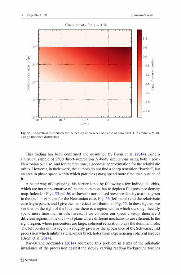
4 Page 86 of 150 P. Amaro-Seoane
−3.6
−3.0
−2.4
−1.8
−1.2
−0.6
0.0
0.6
1.2
log 1
0Presencedensity
10−4 10−3 10−2 10−1
1 − e
10−6
10−5
10−4
10−3
10−2
Semi-m
ajor
axis
a[pc]
Cusp density for γ = 1.75
Fig. 55 Theoretical distribution for the density of presence of a cusp of power-law 1.75 around a MBH,using a truncated distribution
This finding has been confirmed and quantified by Brem et al. (2014) using astatistical sample of 2500 direct-summation N -body simulations using both a post-Newtonian but also, and for the first time, a geodesic approximation for the relativisticorbits. However, in their work, the authors do not find a sharp transition “barrier”, butan area in phase space within which particles (stars) spend more time than outside ofit.
A better way of displaying this barrier is not by following a few individual orbits,which are not representative of the phenomenon, but to depict a full presence densitymap. Indeed, in Figs. 55 and 56, we have the normalised presence density as a histogramin the (a, 1 − e) plane for the Newtonian case, Fig. 56 (left panel) and the relativisticcase (right panel), and I give the theoretical distribution in Fig. 55. In these figures, wesee that on the right of the blue line there is a region within which stars significantlyspend more time than in other areas. If we consider our specific setup, there are 3different regions in the (a, 1−e) plane where different mechanisms are efficient. In theright region, where pericenters are large, coherent relaxation plays the dominant role.The left border of this region is roughly given by the appearance of the Schwarzschildprecession which inhibits stellar-mass black holes from experiencing coherent torques(Brem et al. 2014).
Bar-Or and Alexander (2014) addressed this problem in terms of the adiabaticinvariance of the precession against the slowly varying random background torques
123

Relativistic dynamics and extreme mass ratio inspirals Page 87 of 150 4
−3.2
−2.4
−1.6
−0.8
0.0
0.8
1.6
log 1
0Presencedensity
10−4 10−3 10−2 10−1
1 − e
10−6
10−5
10−4
10−3
10−2
Semi-m
ajor
axis
a[pc]
Newtonian Dynamics
−4.0
−3.2
−2.4
−1.6
−0.8
0.0
0.8
1.6
log 1
0Presencedensity
10−4 10−3 10−2 10−1
1 − e
10−6
10−5
10−4
10−3
10−2
Semi-m
ajor
axis
a[pc]
Dynamics with 1PN, 2PN and 2.5PN
Fig. 56 Integrated presence density for the Newtonian (left panel) and the relativistic case (right panel).The lines indicate the position of the Schwarzschild barrier withCSB = 0.35 (blue) and the limit for captureonto inspiral orbits for non-resonant relaxation (green)
and find that this precession-induced barrier in angular momentum is maximal forsmooth noise. The barrier is not such, nor a reflecting one. It is an effective divisionof phase-space where resonant relaxation is effective, and where it is not.
This interesting and pioneering scenario would obviously imply a priori a severesuppression of EMRI event rates, if we relied on resonant relaxation. While this is truefor EMRIs originating at these distances, the whole picture looks much more differentat larger semi-major axis and eccentricities.
We have seen in Sect. 6.2 that the small compact object will be on a so-called“plunging orbit” if e ≥ eplunge ≡ 1 − 4 RSchw/a. It has been claimed a number oftimes by different authors that this would result in a too short burst of gravitationalradiation which could only be detected if it was originated in our own Galactic Centre(Rubbo et al. 2006; Hopman et al. 2007; Yunes et al. 2008; Berry and Gair 2013)because one needs a coherent integration of some few thousand repeated passagesthrough the periapsis in the LISA bandwidth.
Therefore, such “plunging” objects would then be lost for the GW signal, since theywould be plunging “directly” through the horizon of the MBH and only a final burstof GWs would be emitted, and such burst would be very difficult to recover, since thevery short signal would be buried in a sea of instrumental and confusion noise and theinformation contained in the signal would be practically nil.
However, Amaro-Seoane et al. (2013b) showed that this is not true. Figures 57and 58 show plots of the location of the LSO in the plane a (pc)–(1− e), including theSchwarzschild separatrix between stable and unstable orbits, p−6−2e = 0, for bothprograde and retrograde orbits and for different values of the inclination ι. Each plotcorresponds to a different value of the spin, showing how increasing the spin makes adifference in shifting the location of the separatrix between stable and unstable orbits,pushing prograde orbits near GM•/c2 while retrograde orbits are pushed out towards9GM•/c2. The procedure used to build these plots is a standard one. Briefly, givena value of the dimensionless spin parameter s ≡ a•c2/(GM•) and a value of theeccentricity and inclination angle ι.
123

4 Page 88 of 150 P. Amaro-Seoane
Fig. 57 LSO for a MBH of mass 4 × 10⁴ M� and a SBH of mass m• = 10 M� for a Kerr MBH of spins = 0.4 (left) and s = 0.7 (right). The Schwarzschild separatrix is given as a solid black line. Curves aboveit correspond to retrograde orbits and inclinations of ι = 5.72, 22.91, 40.10, 57.29, 74.48 and 89.95◦starting from the last value (89.95◦). In the left panel we can barely see any difference from the differentinclinations due to the low value of the spin
Fig. 58 The same as in Fig. 57 but for a spin of s = 0.99 (left) and s = 0.999 (right panel). The larger thespin, the “further away” the Kerr LSO gets from the Schwarzschild LSO
Amaro-Seoane et al. (2013b) estimated that the number of cycles that certain EMRIorbital configurations, which were thought to be plunging orbits (or orbits with no suf-ficient cycles), in the case of non-spinning MBHs, can spend in a frequency regime off ∈ [10−4, 1] Hz during their last year(s) of inspiral before plunging into the MBH.This is important to assess how many of these EMRIs will have sufficient Signal-to-Noise Ratio (SNR) to be detectable. It was found that (prograde) EMRIs that are in a“plunge” orbit actually spend a significant number of cycles, more than sufficient tobe detectable with good SNR. The number of cycles has been associated with Nϕ (the
123

Relativistic dynamics and extreme mass ratio inspirals Page 89 of 150 4
number of times that the azimuthal angle ϕ advances 2π ) which is usual for binary sys-tems. However, as I have discussed above, the structure of the waveforms from EMRIsis quite rich since they contain harmonics of three different frequencies. Therefore,the waveforms have cycles associated with the three frequencies ( fr , fθ , fϕ) whichmakes them quite complex and in principle this is good for detectability (assumingwe have the correct waveform templates). Moreover, these cycles happen just beforeplunge and take place in the strong field region very near the MBH horizon. Then,these cycles should contribute more to the SNR than cycles taking place farther awayfrom the MBH horizon.
The authors also estimate the impact on the event rates. Since “direct plunges” areactually disguised EMRIs, although with a higher eccentricity. They prove that
aKerrEMRI
aSchwEMRI
= W−5
6−2γ (ι, s) (97)
NKerrEMRI
NSchwEMRI
= W20γ−4512−4γ (ι, s). (98)
Here, W is a function that depends on ι, the inclination of the EMRI and s, its spin.16
I also have assumed that the stellar-mass black holes distribute around the centralMBH following a power-law cusp of exponent γ , i.e., that the density profile followsρ ∝ r−γ within the region where the gravity of the MBH dominates the gravity of thestars, with γ ranging between 1.75 and 2 for the heavy stellar components (Peebles1972; Bahcall and Wolf 1976, 1977; Amaro-Seoane et al. 2004; Preto et al. 2004;Alexander and Hopman 2009; Preto and Amaro-Seoane 2010; Amaro-Seoane andPreto 2011) (see Gurevich 1964 for an interesting first idea of this concept).17 Forinstance, for a spin of s = 0.999 and an inclination of ι = 0.4 rad, they estimate thatW ∼ 0.26 and, thus, NKerr
EMRI ∼ 30.To sum up, the existence of the barrier prevents “traditional EMRIs” from approach-
ing the central MBH, but if the central MBH is spinning the rate will be dominatedby highly-eccentric extreme mass ratio inspirals anyway, which insolently ignore thepresence of the barrier, because they are driven by chaotic two-body relaxation.
7.7 Extended stars EMRIs
In this section, I review the idea described in Freitag (2003b) that MS stars can bepotential sources of GWs in our Galactic Centre. I include this in this section becausein the whole review our standard CO is considered to be a SBH and so, it falls into thecategory of “not in the standard model”.
Indeed, a MS star can reach close enough distances to the central MBH dependingon its average density and stellar structure. For a mass of around 0.07 M�, the density
16 For the derivation and some examples of values for W , I refer the reader to Amaro-Seoane et al. (2013b).17 The authors obtained a similar solution for how electrons distribute around a positively charged Coulombcentre.
123
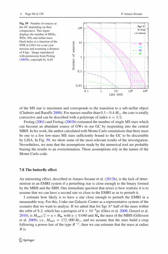
4 Page 90 of 150 P. Amaro-Seoane
Fig. 59 Number of sources atthe GC depending on theircompactness. This figuredisplays the number of MSSs,WDs, NSs and stellar-massblack holes as a function of theSNR in LISA for a one yearmission and assuming a distanceof 8 kpc. Image reproducedwith permission from Freitag(2003b), copyright by AAS
of the MS star is maximum and corresponds to the transition to a sub-stellar object(Chabrier and Baraffe 2000). For masses smaller than 0.3−0.4 M�, the core is totallyconvective and can be described with a polytrope of index n = 3/2.
Freitag (2001) and Freitag (2003b) estimated the number of single MS stars whichcan become an abundant source of GWs in our GC by inspiraling into the centralMBH. In his work, the author calculated with Monte Carlo simulations that there mustbe one to a few low-mass MS stars sufficiently bound to the GC to be discernibleby LISA. In Fig. 59, we show some of the most relevant results of the investigation.Nevertheless, we note that the assumptions made by the numerical tool are probablybiasing the results to an overestimation. These assumptions rely in the nature of theMonte Carlo code.
7.8 The butterfly effect
An interesting effect, described in Amaro-Seoane et al. (2012b), is the lack of deter-minism in an EMRI system if a perturbing star is close enough to the binary formedby the MBH and the SBH. One immediate question that arises is how realistic it is toassume that we can have a second star so close to the EMRI so as to perturb it.
I estimate how likely is to have a star close enough to perturb the EMRI in ameasurable way. For this, I take our Galactic Centre as a representative system of thescenario that we want to analyse. If we admit that for Sgr A* half of the mass withinthe orbit of S-2, which has a periapsis of 6 × 10⁻⁴pc (Ghez et al. 2008; Genzel et al.2010), is Mencl/2 = η × M•, with η ≤ 0.040 and M• the mass of the MBH (Gillessenet al. 2009), i.e., Mencl = 172, 000 M�, and we assume that the stars build a cuspfollowing a power-law of the type R−γ , then we can estimate that the mass at radiusR is
123

Relativistic dynamics and extreme mass ratio inspirals Page 91 of 150 4
M(R) =∫ R
04πr2ρ(r) dr ∝
∫ R
0r−γ+2dr ∝ R3−γ , (99)
for γ < 3. Hence, the number of stars within a sphere of radius R is given by
N (R) � 8.6 × 10⁴(
R
6 × 10⁻⁴ pc
)3−γ
. (100)
And so, the radius within we can expect to find in average a star is
R1 � 6 × 10⁻⁴ pc ×(
1
8.6 × 10⁴
) 13−γ
. (101)
We note, however, that the value derived for η is not observational. As a matter of fact,with current limitations in the observations, it is impossible to know whether all massenclosed by the orbit of S-2 corresponds to the MBH or it contains also an “extended”component. Hence, in order to obtain η, one has to model the system by admittingthat it consists of a punctual source (the MBH) along with a stellar component whoseproperties are parametrised by following a model, not an observation. Figure 60 showsthe dependence on γ of R1. We can see that R1 � 3×10⁻⁷ pc for γ = 1.5 or 7×10⁻⁸
pc for γ = 1.75, see Amaro-Seoane et al. (2004), Freitag et al. (2006b), Preto et al.(2004). These distances are of the same order of magnitude than an EMRI, which iswithin the bandwidth of a LISA-like observatory. Even if this argument is based onthe concept of a cusp and, hence, it is difficult to define at such short radii, in mywork with Marc Freitag and Vassiliki Kalogera (Freitag et al. 2006b) we derive in ourMilky Way-like G25 model some 15 M� within 3 × 10⁻⁴ pc. It is possible that atsuch distances the mass density is totally dominated by stellar-mass black holes, butthe work of Freitag et al. (2006b) does not allow one to resolve them for distancesshorter than 0.01 pc. In this case, strong mass segregation would play a crucial role(Alexander and Hopman 2009; Preto and Amaro-Seoane 2010; Amaro-Seoane andPreto 2011), since for the kind of slopes that one can expect in the case the density isdominated by stellar-mass black holes, the “one-star” radius is much shorter.
In Fig. 61, we have the initial setup for the fiducial case by Amaro-Seoane et al.(2012b). The mass of the MBH is assumed to be M• = 106 M�, the initial semi-majoraxis of the EMRI of a•, i � 1.45×10⁻⁶ pc (i.e., it is well within the band of LISA) , themass of the EMRI is m• = 10 M� (but they also successfully tested 5 and 1.44 M�),the mass of the perturbing star is of m� = 10 M�, the initial semi-major axis of thestar a�, i � 4.1 × 10⁻⁶ pc, and the initial eccentricity e�, i = 0.5 and the inclination isi•, � = 30◦ at T = 0.
We find that the interloper introduces an observable modification in the orbit ofthe EMRI when using a code that uses loss of energy via gravitational radiation atperiapsis. The interesting result, though, is that when taking into account also the twofirst-order non-dissipative post-Newtonian contributions, the orbital evolution is notdeterministic. We do not know what the stellar distribution around a MBH is at suchshort radii, but if this scenario was possible, then the detection of EMRIs would bemuch more challenging than it was thought, because the waveforms developed for
123

4 Page 92 of 150 P. Amaro-Seoane
Fig. 60 Evolution of theone-star radius as a function ofthe slope as in Eq. (101). We cansee that for very mild slopes andeven a core the distances arewithin a millihertzgravitational-wave detectorsimilar to LISA; i.e., of orbitalperiods of 105 s. In this regimewe expect sources of GWs. Forinstance, an EMRI of 10 M�with a MBH of 4 × 10⁶M� hasa semi-major axis of abouta• ≈ 8 × 10⁻⁴ pc and is wellwithin the bandwidth
Fig. 61 Description of thescenario for the butterfly effectby Amaro-Seoane et al. (2012b)(adapted from a figure by LucasSnyder)
detection would be of little use. There has also been work about the role of a massiveperturber on an EMRI. I refer the reader to Chen et al. (2011), Yunes et al. (2011), Seto(2012).
7.9 Role of the gas
Another proposal is related to the presence of massive accretion discs around MBHs.At distances of ∼ 0.1−1 pc from the MBH and with typical accretion rates, thesediscs can be unstable to star formation (Collin and Zahn 1999; Levin and Beloborodov2003; Goodman 2003; Goodman and Tan 2004; Milosavljevic and Loeb 2004; Levin2003, 2006; Nayakshin 2006). If, as in some calculations, there is a bias towards theproduction of massive stars in the disc, they could evolve to become black holes, whichare then dragged in along with the disc matter. Alternately, massive stars on orbits thatcross the disc could be captured and then evolve into black holes (Syer et al. 1991;Rauch 1995; Šubr and Karas 1999; Karas and Šubr 2001). Rates are highly uncertainas well as the mass of the stellar remnants formed (which could even be IMBHs).However these events would likely have a different signature waveform than those ofthe other two classes because they should occur on co-rotating, circular orbits lying
123
Relativistic dynamics and extreme mass ratio inspirals Page 93 of 150 4
in the equatorial plane of the spinning MBH if it has gained a significant fraction ofits mass by accreting from the disc (Bardeen 1970; King et al. 2005; Volonteri et al.2005). Moreover, there is the exciting possibility that in such a scenario the compactobject would open a gap in the disc, which could lead to an optical counterpart to theEMRI event (Levin 2006).
Barausse et al. (2007) address the imprint on the waveform of compact, massive toriclose to the central MBH. The kludge waveforms generated in their study were indis-tinguishable from pure Kerr waveforms in the regime on which they focused. Barausseand his collaborators later extended the study to a non self-gravitating torus with con-stant specific angular momentum and found that typically one should not expect bigdifferences, although for a certain region of the parameter space the hydrodynamicdrag acting on the EMRI does have an impact comparable to the radiation-reaction,so that it could, in principle, be measurable (Barausse and Rezzolla 2008). Later, thiswork was expanded in Barausse et al. (2014). Nevertheless, it is not clear what theappropriate gas distribution around the MBH is in the regime of their study. Pertur-bations to the SBH are likely to be negligible if accretion onto the hole happens ina low density, radiatively inefficient flow. Such flows are much more common thandense accretion discs, which in principle could yield observable phase shifts duringthe inspiral (Kocsis et al. 2011), at least within the redshift range in which we expectto observe EMRIs.
8 Integration of dense stellar systems and EMRIs
8.1 Introduction
In this section, we give a summary of the current numerical approaches available forstudying stellar dynamics in systems for which relaxation is an important factor.18
As of writing this article, only approximate methods using a number of simplifyingassumptions have been used to estimate the rates and characteristics of EMRIs. Ireview these approaches, their accomplishments and limitations. Thanks to the rapidcomputational power increase and the development of new algorithms, it is most likelythat direct N -body techniques will soon be able to robustly confirm or disprove theseapproximate results and extend them. One of the main issues is that exceptionally longand accurate integrations are required to account correctly for secular effects such ascoherent relaxation or Kozai oscillations. These requirements, and the extreme massratio pose new challenges to developers of N -body codes.
We can approximately classify the different kinds of techniques employed forstudying stellar dynamics according to the dynamical regime(s) they can cope with.In Fig. 62 we have a classification of these techniques. (Semi-)analytical methodsare generally sufficient only to study systems which are in dynamical equilibriumand which are not affected by collisional (relaxational) processes. In all other cases,including those of importance for EMRI studies, the complications that arise if we
18 A part of this section profits from Amaro-Seoane et al. (2007), though some parts have been significantlyexpanded and improved.
123
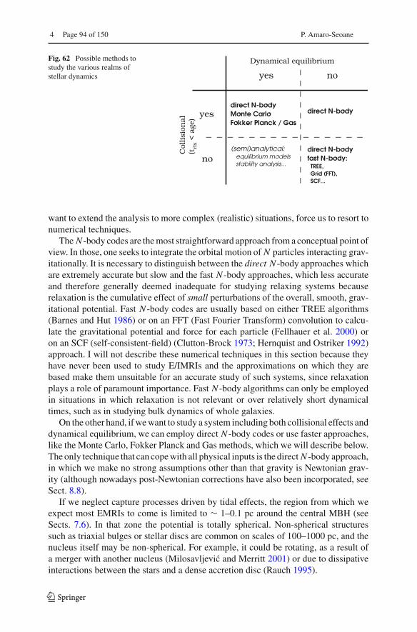
4 Page 94 of 150 P. Amaro-Seoane
Fig. 62 Possible methods tostudy the various realms ofstellar dynamics
want to extend the analysis to more complex (realistic) situations, force us to resort tonumerical techniques.
The N -body codes are the most straightforward approach from a conceptual point ofview. In those, one seeks to integrate the orbital motion of N particles interacting grav-itationally. It is necessary to distinguish between the direct N -body approaches whichare extremely accurate but slow and the fast N -body approaches, which less accurateand therefore generally deemed inadequate for studying relaxing systems becauserelaxation is the cumulative effect of small perturbations of the overall, smooth, grav-itational potential. Fast N -body codes are usually based on either TREE algorithms(Barnes and Hut 1986) or on an FFT (Fast Fourier Transform) convolution to calcu-late the gravitational potential and force for each particle (Fellhauer et al. 2000) oron an SCF (self-consistent-field) (Clutton-Brock 1973; Hernquist and Ostriker 1992)approach. I will not describe these numerical techniques in this section because theyhave never been used to study E/IMRIs and the approximations on which they arebased make them unsuitable for an accurate study of such systems, since relaxationplays a role of paramount importance. Fast N -body algorithms can only be employedin situations in which relaxation is not relevant or over relatively short dynamicaltimes, such as in studying bulk dynamics of whole galaxies.
On the other hand, if we want to study a system including both collisional effects anddynamical equilibrium, we can employ direct N -body codes or use faster approaches,like the Monte Carlo, Fokker Planck and Gas methods, which we will describe below.The only technique that can cope with all physical inputs is the direct N -body approach,in which we make no strong assumptions other than that gravity is Newtonian grav-ity (although nowadays post-Newtonian corrections have also been incorporated, seeSect. 8.8).
If we neglect capture processes driven by tidal effects, the region from which weexpect most EMRIs to come is limited to ∼ 1–0.1 pc around the central MBH (seeSects. 7.6). In that zone the potential is totally spherical. Non-spherical structuressuch as triaxial bulges or stellar discs are common on scales of 100–1000 pc, and thenucleus itself may be non-spherical. For example, it could be rotating, as a result ofa merger with another nucleus (Milosavljevic and Merritt 2001) or due to dissipativeinteractions between the stars and a dense accretion disc (Rauch 1995).
123
Relativistic dynamics and extreme mass ratio inspirals Page 95 of 150 4
It is unclear whether this effect could enhance the replenishment of the loss cone,see Murphy et al. (1991), Freitag and Benz (2002), Amaro-Seoane et al. (2004),Baumgardt et al. (2004a, b), Merritt and Vasiliev (2011), Vasiliev and Merritt (2013);and Vasiliev et al. (2014) in particular for the even more complex of binaries of massiveblack holes, in the context of the “final parsec problem”. The problem is furthercompounded, for example, by the presence of multiple stellar populations whosespatial distributions are segregated (“mass segregation”), with more massive starssinking deeper into the potential well and approaching closer to the central black hole.Besides, two interacting stars may become gravitationally bound (become a binary)so that during the subsequent interactions with other stars or massive black holes theybehave differently from single stars, or they may collide into each other, then thesubsequent evolution will be determined by gas-dynamics. As these “micro-physical”effects are usually not incorporated into the global modeling of the entire nuclear starclusters, considerable uncertainties are attached to the theoretical predictions of theabundance and orbital parameters of the stars in the relativistic regime.
Whilst assuming sphericity will probably not have any impact on the estimate ofcapture rates, it is of huge relevance for “tidal processes”, since this is the region inwhich binary tidal separation and the tidal capture of giant cores will happen. Forthese processes the critical radius is beyond the influence radius of the central MBHand so triaxiality can probably play an important role. Due to computer power andthe limitations of simulation codes, galactic nuclei have so far been modelled only asisolated spherical clusters with purely Newtonian gravity (e.g., Murphy et al. 1991;Freitag and Benz 2002). Vasiliev (2015) used the Princeton approach to derive a newMonte Carlo code, which presents a scheme to deal with asphericity (with other issuesremaining open), with the limitation that it assumes isotropy of background starspopulation, so that it cannot model a highly flattened system with significant rotationsupport.
More realistic situations could only be explored with N -body methods or possi-bly with hybrid codes (Monte Carlo combined with N -body, for instance). Whileimportant approaches exist that implement small-number N -body integrations in thecore of Monte Carlo, see Hypki and Giersz (2013), Fregeau and Rasio (2007), theseapproaches typically focus on binary scattering interactions, with less than five bodies.An important exception is the work of Rodriguez et al. (2015), which can integratelarger numbers, but it is limited to CPUs. Being based on KIRA (Portegies Zwartet al. 2001), it can in principle run on GRAPEs, a special-purpose chip to computegravitational forces that was used in the past by many groups, see e.g., Fukushige et al.(2005), but (i) it is fair to say that these cards are obsolete, and virtually all effortsfocus now on GPUs (there exists a library that can allow a GRAPE to mimic a GPU(Gaburov et al. 2009), but it is far from trivial to do it and in any case sub-optimal),(ii) it does not account for relativistic corrections, crucial to EMRI astrophysics, (iii)the code requires spherical symmetry and (iv) the code does not account for a centralMBH.
Figure 63 shows a schematic illustration of the current available codes for stel-lar dynamics including relaxation. The physical realism of the codes increases fromthe left to the right while the computational speed decreases. The two-dimensionalnumerical direct solutions of the Fokker–Planck equation (Takahashi 1997, 1996,
123

4 Page 96 of 150 P. Amaro-Seoane
Fig. 63 The various methods used to study collisional stellar dynamics. In the case of direct N -bodycomputations, the simulations require the use of either special-purpose hardware such as the GRAPEs,Beowulf clusters for the parallel version of Rainer Spurzem or Graphical Computing Units (GPUs). Aversion of the parallel code N -body6++ ported to GPU architecture has been developed, see Wang et al.(2015, 2016), which allows us to simulate more realistic particles numbers
1995) probably require the least computational time, but these are followed closely bythe gaseous model. The idea behind it is to treat two-body relaxation as a transport pro-cess such as in a conducting plasma (Hachisu et al. 1978; Lynden-Bell and Eggleton1980). Multi-mass models have been implemented(Louis and Spurzem 1991; Spurzem1992; Giersz and Spurzem 1994; Spurzem and Takahashi 1995) and improved for thedetailed form of the conductivities by comparing to direct N -body models (describedbelow). The addition of a central accreting MBH and a treatment for loss-cone effectswas done by Amaro-Seoane et al. (2004) (a comprehensive description of the codeis in the appendix of the same work) for the single-mass case, and also for a stel-lar mass spectrum (Amaro-Seoane 2004). The advantage of these two codes is thecomputational time required to perform a simulation (typically of the order of oneminute on a regular PC for a Hubble time) and since they are not particle-based, theresolution can be envisaged as infinite, so that they are not limited by the particle num-ber of the system and there is practically no numerical noise. Nevertheless, althoughthey should be envisaged as powerful tools to make an initial, fast exploration of theparameter space, the results give us tendencies of the system, rather than an accurateanswer (Amaro-Seoane 2004). Studying the astrophysical I/EMRI problem requires ameticulous characterisation of the orbital parameters, so that approximate techniquesshould be regarded as exploratory only (de Freitas Pacheco et al. 2006).
123
Relativistic dynamics and extreme mass ratio inspirals Page 97 of 150 4
8.2 The Fokker–Planck approach
Instead of tracking the individual motion of a large number of particles, as in N -bodymethods, one can attempt to describe a system consisting of a very large number ofstars through the 1-particle phase-space distribution function (DF for short) f (x, v, t).The best interpretation of f , with the proviso that it has been properly normalised, isas a probability density if it is normalised to 1— f (x, v, t)d3x d3v is the probability offinding, at time t , any given particle within the volume of phase space d3x d3v aroundthe 6-D phase-space point (x, v); the average number of particles in this volume wouldbe N� f (x, v, t)d3x d3v, with N� the total number of particles. If the particles movein a common smooth potential Φ, the evolution of f is described by the collisionlessBoltzmann equation (Binney and Tremaine 1987):
Dt f ≡ ∂ f
∂t+ v · ∇ f − ∇Φ · ∂ f
∂v= 0. (102)
Φ is obtained from f and a possible external potential Φext (such as the one producedby a central MBH) from the Poisson equation.
In a real self-gravitating N -particle system the potential cannot be smooth onsmall scales but has some graininess, i.e., short-term, small-scale fluctuations, Φreal =Φ + ΔΦgrainy. Relaxation describes the effects of these fluctuations on f . They arisebecause a given particle sees the rest of the system as a collection of point massesrather than as a smooth mass distribution. Relaxational effects, also known (some-what confusingly) as collisional effects, can therefore be seen as particles influencingeach other individually as opposed as to collectively. To allow for these effects, acollision term has to be introduced on the right-hand side of the Boltzmann equation,in Eq. (102). This equation cannot be equated to zero if we want to take into accountrelaxational effects. The Fokker–Planck (FP) equation is derived by assuming thatrelaxation is due to a large number of 2-body gravitational encounters, each of whichleads to a small deflection and occurs “locally”, i.e., they affect the velocity of a starwithout affecting its position. This is the basis for Chandrasekhar’s theory of relax-ation (Chandrasekhar 1960; Binney and Tremaine 1987; Spitzer Jr 1987). To take careof encounters between stars, hence, we have to equate Eq. (102) not to zero, but to acollision term,
Dt f = −3∑
i=1
∂
∂vi[ f (x, v)〈Δvi 〉] + 1
2
3∑i, j=1
∂2
∂vi∂v j
[f (x, v)〈ΔviΔv j 〉
], (103)
where the “diffusion coefficient” 〈Δvi 〉 is the average change in vi per unit of time dueto encounters (see Rosenbluth et al. 1957; Binney and Tremaine 1987 for a derivation).
From Jeans’ theorem (Jeans 1915; Merritt 1999), for a spherical system in dynam-ical equilibrium, the DF f can depend on the phase-space coordinates (x, v) onlythrough the (specific) orbital binding energy E and angular momentum (in modulus)J ,
f (x, v) = F(E(x, v), J (x, v)). (104)
123
4 Page 98 of 150 P. Amaro-Seoane
In the vast majority of applications, the Fokker–Planck formalism is applied in thetwo-dimensional (E, J )-space or, assuming isotropy, the one-dimensional energy-space rather than the six-dimensional phase space, through the operation of “orbitaveraging” (see Cohn 1979, 1980, 1985; Spitzer Jr 1987 amongst others).
A standard form of the FP equation for an isotropic, spherical system is
Dt N (E) ≡ ∂N
∂t+ ∂N
∂E
dE
dt
∣∣∣∣φ
= −∂FE
∂E(105)
where
FE = mDE F − DEE∂F
∂E(106)
is the flux of particles in the energy space; dE/dt |φ is the change of energy due tothe evolution of the potential φ; N (E) is the density of stars in E−space,
N (E) = 16π2 p(E)F(E) (107)
with
p(E) =∫ rmax
0r2v dr. (108)
The “flux coefficients” are
DE = 16π3λmf
∫ E
φ(0)
dE ′ p(E ′)Ff(E′), (109)
DEE = 16π3λm2f
[q(E)
∫ 0
EdE ′Ff(E
′) +∫ E
φ(0)
dE ′q(E ′)Ff(E′)], (110)
where λ ≡ 4πG2 ln Λ and q(E) = 13
∫ rmax0 r2v3 dr is the volume of phase space
accessible to particles with energies lower than energy, and p(E) = ∂q/∂E (Goodman1983).
We use an index “f” for “field” to distinguish the mass and DF of the populationwe follow (“test-stars”) from the “field” objects. This distinction does not apply to asingle-component system but it is easy to generalise to a multi-component situationby summing over components to get the total flux coefficient
DE =Ncomp∑l=1
DE ,l , DEE =Ncomp∑l=1
DEE ,l , (111)
where the flux coefficient for component l can written by replacing the subscript “f”by “l” in Eq. (110).
I now explain schematically how the FP equation is implemented numerically tofollow the evolution of star clusters. A more detailed description can be found in,e.g., Chernoff and Weinberg (1990). In the most common scheme, pioneered by Cohn(1980), two types of steps are employed alternately, a method known as “operatorsplitting”:
123

Relativistic dynamics and extreme mass ratio inspirals Page 99 of 150 4
1. Diffusion step. The change in the distribution function F for a discrete time-stepΔt is computed by using the FP equation assuming the potential φ is fixed, i.e.,setting Dt N = ∂N/∂t = ∂N/∂t |coll. The FP equation is discretized on an energygrid. The flux coefficients are computed using the DF(s) of the previous step;this makes the equations linear in the values of F on the grid points. The finite-differencing scheme is the implicit Chang and Cooper (1970) algorithm, based ona finite difference scheme for initial value problems, which is first order in timeand energy.
2. Poisson step. Now, the change of potential resulting from the modification inthe DF F is computed and F is modified to account for the term dE/dt |φ , i.e.,assuming Dt N = ∂N/∂t + ∂N/∂E dE/dt |φ = 0. This can be done implicitlybecause, as long as the change in φ over Δt is very small, the actions of each orbitare adiabatic invariants. Hence, during the Poisson step, the distribution function,expressed in terms of the actions, does not change. In practice, an iterative schemeis used to compute the modified potential, determined implicitly by the modifiedDF, through the Poisson equation. The iteration starts with the values of φ, ρ, etc.computed before the previous diffusion step.
A variant of the FP equation analogous to Eq. (105) can be written, which allowsfor anisotropy by taking into account the dependence of F on angular momentumand including a angular momentum-flux and corresponding flux coefficients (Cohnand Kulsrud 1978; Cohn 1979, 1985; Takahashi 1995, 1996, 1997; Drukier et al.1999). The expressions for the flux coefficients are significantly longer than in theisotropic case and I do not present them here. However, we note that in galactic nuclei,in contrast to globular clusters, anisotropy plays a key role because of the existenceof a loss cone.
The use of the FP approach to determine the distribution of stars around a MBHrequires a few modifications. First the (Keplerian) contribution of the MBH to thepotential has to be added. Several authors have made use of the FP or similar formalismsto study the dynamics well within the influence radius under the assumption of afixed potential (Bahcall and Wolf 1976, 1977; Lightman and Shapiro 1977; Cohnand Kulsrud 1978; Hopman and Alexander 2006b, a; Merritt et al. 2006), which is asignificant simplification. The static potential included a contribution for the stellarnucleus in the last study (Merritt et al. 2006) but was limited to a Keplerian MBHpotential in the other cases. The presence of the MBH also constitutes a central sinkas stars are destroyed or swallowed if they come very close to it. This has to beimplemented into FP codes as a boundary condition. Lightman and Shapiro (1977)and Cohn and Kulsrud (1978) have developed detailed (and rather complex) treatmentsof the loss cone for the anisotropic FP formalism. It can be used in a simplified wayin an isotropic FP analysis (Bahcall and Wolf 1977) to obtain a good approximationto the distribution of stars around a MBH and of the rates of consumption of starsby the MBH. However, additional analysis is required to determine what fraction ofthe swallowed stars are EMRIs and what their orbital properties are (Hopman andAlexander 2005, 2006a).
123
4 Page 100 of 150 P. Amaro-Seoane
8.3 Moment models
Another way to approximately solve the (collisional) Boltzmann equation is to takevelocity moments of it. The moment or order n = 0 of the DF is the density, themoments of order n = 1 are bulk velocities and n = 2 corresponds to (anisotropic)pressures (or velocity dispersions). This is analogous to the derivation of the Jeansequation from the collisionless Boltzmann equation (Binney and Tremaine 1987) butthe collision term introduces moments of order n + 1 in the equations for moments oforder n.
In statistical moment models, we employ velocity moments to characterise thelocal velocity distribution function. The n-th moment of a velocity distribution f (v)
is defined as 〈vn〉 = ∫(v)n f (v) dv. The accuracy of these models is then limited
by the order of the highest moment included to describe the velocity distribution, asdiscussed in detail in Schneider et al. (2011).
Since each stellar dynamical process driving the evolution of a cluster has a differentimpact on the local velocity distribution, this motivates us to construct a distributionfunction that is able to reflect the effects of each of these processes properly so asnot to lose information that influences the clusters evolution. The velocity distributioncan be written as a series expansion using a truncated Gauss–Hermite series, as inGerhard (1993), van der Marel and Franx (1993) to illustrate the meaning of the firstfour moments:
f (vr ) ∝ exp
(−vr − vr
2σ
)[1 +
4∑k=3
hk Hk(vr − vr )
], (112)
where Hk are the Hermite polynomials (see, e.g., the Appendix A of van der Mareland Franx 1993), vr the velocity in radial direction (or the line-of-sight velocity whichis the velocity measured in direction of an observer), and vr , σ , h3 and h4 are freeparameters. The first moments can be related to physical properties of the system thatwe are studying:
0th moment: The zeroth moment of a velocity distribution is 1 due to normalisation.1st moment: The first moment of a velocity distribution is the mean velocity vr and
denotes the bulk mass transport velocity.2nd moment: The second moment of a velocity distribution is the variance σ and is
equal to the velocity dispersion. It determines the width of f (vr ) andthus the scattering of stellar velocities around the mean velocity vr . Iff (vr ) is fully determined by vr and σ and h3 = h4 = 0 it is a Gaussian(upper left panel in Fig. 64) corresponding to thermal equilibrium. Thenthe symmetry of the one-dimensional velocity distribution f (vr ) to vrreflects isotropy.
3rd moment: The third moment, denotes the transport of random kinetic energy anddepends on h3. If the third moment of the velocity distribution does notvanish, implying that h3 �= 0, then the shape of the velocity distribu-tion is a skewed Gaussian (Fig. 64, upper right panel). The asymmetry
123
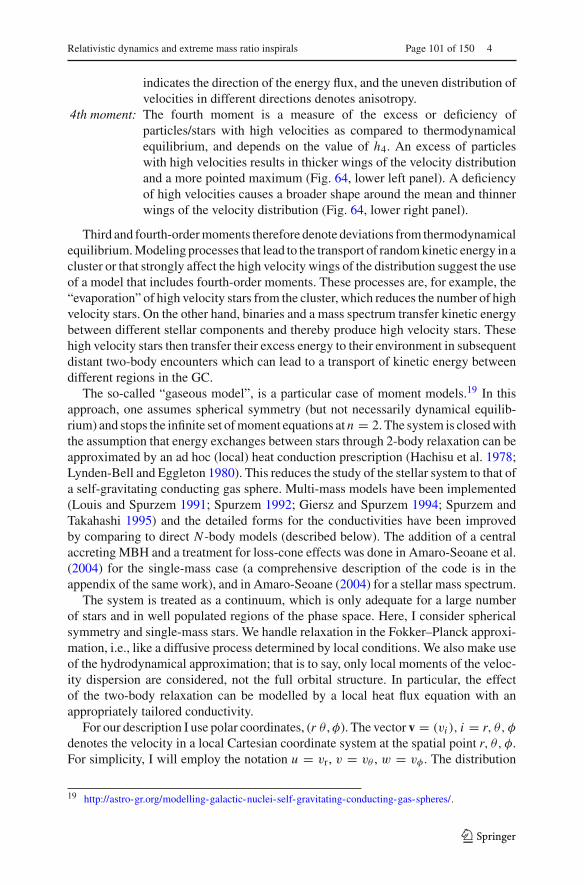
Relativistic dynamics and extreme mass ratio inspirals Page 101 of 150 4
indicates the direction of the energy flux, and the uneven distribution ofvelocities in different directions denotes anisotropy.
4th moment: The fourth moment is a measure of the excess or deficiency ofparticles/stars with high velocities as compared to thermodynamicalequilibrium, and depends on the value of h4. An excess of particleswith high velocities results in thicker wings of the velocity distributionand a more pointed maximum (Fig. 64, lower left panel). A deficiencyof high velocities causes a broader shape around the mean and thinnerwings of the velocity distribution (Fig. 64, lower right panel).
Third and fourth-order moments therefore denote deviations from thermodynamicalequilibrium. Modeling processes that lead to the transport of random kinetic energy in acluster or that strongly affect the high velocity wings of the distribution suggest the useof a model that includes fourth-order moments. These processes are, for example, the“evaporation” of high velocity stars from the cluster, which reduces the number of highvelocity stars. On the other hand, binaries and a mass spectrum transfer kinetic energybetween different stellar components and thereby produce high velocity stars. Thesehigh velocity stars then transfer their excess energy to their environment in subsequentdistant two-body encounters which can lead to a transport of kinetic energy betweendifferent regions in the GC.
The so-called “gaseous model”, is a particular case of moment models.19 In thisapproach, one assumes spherical symmetry (but not necessarily dynamical equilib-rium) and stops the infinite set of moment equations at n = 2. The system is closed withthe assumption that energy exchanges between stars through 2-body relaxation can beapproximated by an ad hoc (local) heat conduction prescription (Hachisu et al. 1978;Lynden-Bell and Eggleton 1980). This reduces the study of the stellar system to that ofa self-gravitating conducting gas sphere. Multi-mass models have been implemented(Louis and Spurzem 1991; Spurzem 1992; Giersz and Spurzem 1994; Spurzem andTakahashi 1995) and the detailed forms for the conductivities have been improvedby comparing to direct N -body models (described below). The addition of a centralaccreting MBH and a treatment for loss-cone effects was done in Amaro-Seoane et al.(2004) for the single-mass case (a comprehensive description of the code is in theappendix of the same work), and in Amaro-Seoane (2004) for a stellar mass spectrum.
The system is treated as a continuum, which is only adequate for a large numberof stars and in well populated regions of the phase space. Here, I consider sphericalsymmetry and single-mass stars. We handle relaxation in the Fokker–Planck approxi-mation, i.e., like a diffusive process determined by local conditions. We also make useof the hydrodynamical approximation; that is to say, only local moments of the veloc-ity dispersion are considered, not the full orbital structure. In particular, the effectof the two-body relaxation can be modelled by a local heat flux equation with anappropriately tailored conductivity.
For our description I use polar coordinates, (r θ , φ). The vector v = (vi ), i = r, θ, φ
denotes the velocity in a local Cartesian coordinate system at the spatial point r, θ, φ.For simplicity, I will employ the notation u = vr, v = vθ , w = vφ . The distribution
19 http://astro-gr.org/modelling-galactic-nuclei-self-gravitating-conducting-gas-spheres/.
123
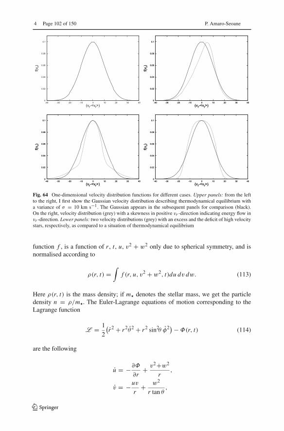
4 Page 102 of 150 P. Amaro-Seoane
0
0.02
0.04
0.06
0.08
0.1
-40 -30 -20 -10 0 10 20 30 40
f(vr)
(vr-<vr>) 0
0.02
0.04
0.06
0.08
0.1
-40 -30 -20 -10 0 10 20 30 40
f(vr)
(vr-<vr>) 0
0.02
0.04
0.06
0.08
0.1
-40 -30 -20 -10 0 10 20 30 40
f(vr)
(vr-<vr>)
0
0.02
0.04
0.06
0.08
0.1
-40 -30 -20 -10 0 10 20 30 40
f(vr)
(vr-<vr>) 0
0.02
0.04
0.06
0.08
0.1
-40 -30 -20 -10 0 10 20 30 40
f(vr)
(vr-<vr>) 0
0.02
0.04
0.06
0.08
0.1
-40 -30 -20 -10 0 10 20 30 40
f(vr)
(vr-<vr>) 0
0.02
0.04
0.06
0.08
0.1
-40 -30 -20 -10 0 10 20 30 40
f(vr)
(vr-<vr>)
Fig. 64 One-dimensional velocity distribution functions for different cases. Upper panels: from the leftto the right, I first show the Gaussian velocity distribution describing thermodynamical equilibrium witha variance of σ = 10 km s−1. The Gaussian appears in the subsequent panels for comparison (black).On the right, velocity distribution (grey) with a skewness in positive vr -direction indicating energy flow invr -direction. Lower panels: two velocity distributions (grey) with an excess and the deficit of high velocitystars, respectively, as compared to a situation of thermodynamical equilibrium
function f , is a function of r , t , u, v2 + w2 only due to spherical symmetry, and isnormalised according to
ρ(r, t) =∫
f (r, u, v2 + w2, t)du dv dw. (113)
Here ρ(r, t) is the mass density; if m� denotes the stellar mass, we get the particledensity n = ρ/m�. The Euler-Lagrange equations of motion corresponding to theLagrange function
L = 1
2
(r2 + r2θ2 + r2 sin2θ φ2)− Φ(r, t) (114)
are the following
u = −∂Φ
∂r+ v2+w2
r,
v = −uv
r+ w2
r tan θ,
123

Relativistic dynamics and extreme mass ratio inspirals Page 103 of 150 4
w = −uw
r− vw
r tan θ. (115)
And so we get a complete local Fokker–Planck equation,
∂ f
∂t+ vr
∂ f
∂r+ vr
∂ f
∂vr+ vθ
∂ f
∂vθ
+ vϕ
∂ f
∂vϕ
=(
δ f
δt
)FP
. (116)
In our model we do not solve the equation directly; we use a so-called momentsprocess. The moments of the velocity distribution function f are defined as follows
〈i, j, k〉 :=∫ +∞
−∞(vr)
i (vθ )j (vφ)k f (r, vr, vθ , vφ, t) dvrdvθdvφ; (117)
Using the previous definition, I introduce now the following moments of the velocitydistribution function,
〈0, 0, 0〉 := ρ =∫
f du dv dw, (118)
〈1, 0, 0〉 := u =∫
u f du dv dw, (119)
〈2, 0, 0〉 := pr + ρu2 =∫
u2 f du dv dw, (120)
〈0, 2, 0〉 := pθ =∫
v2 f du dv dw, (121)
〈0, 0, 2〉 := pφ =∫
w2 f du dv dw, (122)
〈3, 0, 0〉 := Fr + 3upr + u3 =∫
u3 f du dv dw, (123)
〈1, 2, 0〉 := Fθ + upθ =∫
uv2 f du dv dw, (124)
〈1, 0, 2〉 := Fφ + upφ =∫
uw2 f du dv dw, (125)
where ρ is the density of stars, u is the bulk velocity, vr and vt are the radial andtangential flux velocities,
vr = Fr
3pr+ u,
vt = Ft
2pt+ u, (126)
pr and pt are the radial and tangential pressures, Fr is the radial and Ft the tangentialkinetic energy flux (Louis and Spurzem 1991). Note that the definitions of pi and Fiare such that they are proportional to the random motion of the stars. Due to spherical
123
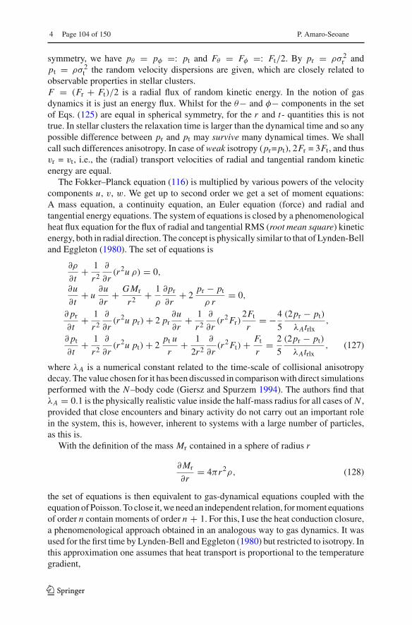
4 Page 104 of 150 P. Amaro-Seoane
symmetry, we have pθ = pφ =: pt and Fθ = Fφ =: Ft/2. By pr = ρσ 2r and
pt = ρσ 2t the random velocity dispersions are given, which are closely related to
observable properties in stellar clusters.F = (Fr + Ft)/2 is a radial flux of random kinetic energy. In the notion of gasdynamics it is just an energy flux. Whilst for the θ− and φ− components in the setof Eqs. (125) are equal in spherical symmetry, for the r and t- quantities this is nottrue. In stellar clusters the relaxation time is larger than the dynamical time and so anypossible difference between pr and pt may survive many dynamical times. We shallcall such differences anisotropy. In case of weak isotropy (pr=pt), 2Fr = 3Ft , and thusvr = vt , i.e., the (radial) transport velocities of radial and tangential random kineticenergy are equal.
The Fokker–Planck equation (116) is multiplied by various powers of the velocitycomponents u, v, w. We get up to second order we get a set of moment equations:A mass equation, a continuity equation, an Euler equation (force) and radial andtangential energy equations. The system of equations is closed by a phenomenologicalheat flux equation for the flux of radial and tangential RMS (root mean square) kineticenergy, both in radial direction. The concept is physically similar to that of Lynden-Belland Eggleton (1980). The set of equations is
∂ρ
∂t+ 1
r2
∂
∂r(r2u ρ) = 0,
∂u
∂t+ u
∂u
∂r+ GMr
r2 + 1
ρ
∂pr
∂r+ 2
pr − pt
ρ r= 0,
∂ pr
∂t+ 1
r2
∂
∂r(r2u pr) + 2 pr
∂u
∂r+ 1
r2
∂
∂r(r2Fr)
2Ft
r= −4
5
(2pr − pt)
λAtrlx,
∂ pt
∂t+ 1
r2
∂
∂r(r2u pt) + 2
pt u
r+ 1
2r2
∂
∂r(r2Ft) + Ft
r= 2
5
(2pr − pt)
λAtrlx, (127)
where λA is a numerical constant related to the time-scale of collisional anisotropydecay. The value chosen for it has been discussed in comparison with direct simulationsperformed with the N–body code (Giersz and Spurzem 1994). The authors find thatλA = 0.1 is the physically realistic value inside the half-mass radius for all cases of N ,provided that close encounters and binary activity do not carry out an important rolein the system, this is, however, inherent to systems with a large number of particles,as this is.
With the definition of the mass Mr contained in a sphere of radius r
∂Mr
∂r= 4πr2ρ, (128)
the set of equations is then equivalent to gas-dynamical equations coupled with theequation of Poisson. To close it, we need an independent relation, for moment equationsof order n contain moments of order n + 1. For this, I use the heat conduction closure,a phenomenological approach obtained in an analogous way to gas dynamics. It wasused for the first time by Lynden-Bell and Eggleton (1980) but restricted to isotropy. Inthis approximation one assumes that heat transport is proportional to the temperaturegradient,
123
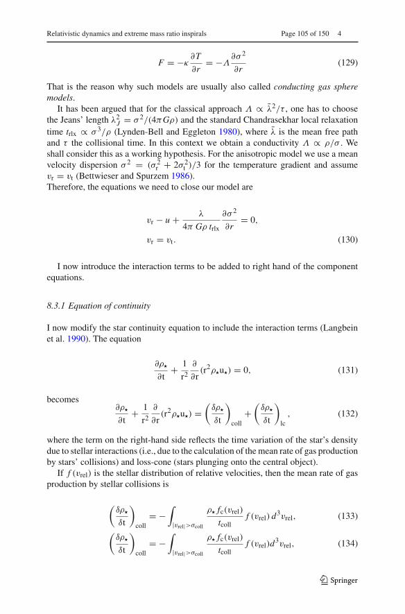
Relativistic dynamics and extreme mass ratio inspirals Page 105 of 150 4
F = −κ∂T
∂r= −Λ
∂σ 2
∂r(129)
That is the reason why such models are usually also called conducting gas spheremodels.
It has been argued that for the classical approach Λ ∝ λ2/τ , one has to choosethe Jeans’ length λ2
J = σ 2/(4πGρ) and the standard Chandrasekhar local relaxationtime trlx ∝ σ 3/ρ (Lynden-Bell and Eggleton 1980), where λ is the mean free pathand τ the collisional time. In this context we obtain a conductivity Λ ∝ ρ/σ . Weshall consider this as a working hypothesis. For the anisotropic model we use a meanvelocity dispersion σ 2 = (σ 2
r + 2σ 2t )/3 for the temperature gradient and assume
vr = vt (Bettwieser and Spurzem 1986).Therefore, the equations we need to close our model are
vr − u + λ
4π Gρ trlx
∂σ 2
∂r= 0,
vr = vt. (130)
I now introduce the interaction terms to be added to right hand of the componentequations.
8.3.1 Equation of continuity
I now modify the star continuity equation to include the interaction terms (Langbeinet al. 1990). The equation
∂ρ�
∂t+ 1
r2
∂
∂r(r2ρ�u�) = 0, (131)
becomes∂ρ�
∂t+ 1
r2
∂
∂r(r2ρ�u�) =
(δρ�
δt
)coll
+(
δρ�
δt
)lc
, (132)
where the term on the right-hand side reflects the time variation of the star’s densitydue to stellar interactions (i.e., due to the calculation of the mean rate of gas productionby stars’ collisions) and loss-cone (stars plunging onto the central object).
If f (vrel) is the stellar distribution of relative velocities, then the mean rate of gasproduction by stellar collisions is
(δρ�
δt
)coll
= −∫
|vrel|>σcoll
ρ� fc(vrel)
tcollf (vrel) d
3vrel, (133)
(δρ�
δt
)coll
= −∫
|vrel|>σcoll
ρ� fc(vrel)
tcollf (vrel)d
3vrel, (134)
123

4 Page 106 of 150 P. Amaro-Seoane
where f (vrel) is a Schwarzschild - Boltzmann distribution,
f (vrel) = 1
2π3/2σrσ2t
exp
[− (vrel,r − u�)
2
4σ 2r
− v2rel,t
2σ 2t
]. (135)
With regards to fc, it is the relative fraction of mass liberated per stellar collision intothe gaseous medium. Under certain assumptions given in the initial work of Spitzer Jrand Saslaw (1966), we can calculate it as an average over all impact parametersresulting in rmin < 2 r� and as a function of the relative velocity at infinity of the twocolliding stars, vrel. Langbein et al. (1990) approximate their result by
fc(vrel) ={(
1 + qcoll
√σcollvrel
)−1vrel > σcoll,
0 vrel < σcoll,(136)
with qcoll = 100. Hence, we have that
fc(vrel) ={
0.01 σcoll = vrel,
0 σcoll > vrel.(137)
The first interaction term is
(δρ�
δt
)coll
= −ρ�
fc
tcoll
[1 − erf
(σcoll√
6σr
)][1 − erf
(σcoll√
6σt
)]2
, (138)
which, for simplification, we call it
(δρ�
δt
)coll
≡ −ρ�Xcoll. (139)
Since the evolution of the system that we are studying can be regarded as stationary,I introduce for each equation the “logarithmic variables” in order to study the long-term evolution. On the other hand, if the system happens to have quick changes, weshould use the “non-logarithmic” version of the equations. For this reason, I will writeat the end of each subsection the equation in terms of the logarithmic variables.
In the case of the equation of continuity, I develop it and divide it by ρ� becausewe are looking for the logarithm of the star density, ∂ ln ρ�/∂t = (1/ρ�)∂ρ�/∂t . Theresult is:
∂ ln ρ�
∂t+ ∂u�
∂r+ u�
∂ ln ρ�
∂r+ 2u�
r= 1
ρ�
(δρ�
δt
)coll
+ 1
ρ�
(δρ�
δt
)lc
(140)
123

Relativistic dynamics and extreme mass ratio inspirals Page 107 of 150 4
8.3.2 Momentum balance equation
The second equation has the following star interaction terms:
∂u�
∂t+ u�
∂u�
∂r+ GMr
r2 + 1
ρ�
∂pr
∂r+ 2
pr − pt
ρ�r=(
δu�
δt
)drag
. (141)
The interaction term is due to the decelerating force that stars moving inside the gasare subject. (
δu�
δt
)drag
= −Xdrag1
ρ�
(u� − ug), (142)
where I have introduced the following definition:
Xdrag ≡ −CDπr2
�
m�
ρ�ρgσtot, (143)
with σ 2tot = σ 2
r + σ 2t + (u� − ug)
2. In the “gaseous model”, I use a logarithmicexpression of the equation, so that we multiply Eq. (141) by ρ�r/pr:
ρ�r
pr
(∂u�
∂t+ u�
)+GMr
rprρ�+∂ ln pr
∂ ln r+2
(1 − pt
pr
)= −Xdrag
r
pr
(u� − ug
). (144)
8.3.3 Radial energy equation
Regarding the penultimate equation, the interaction terms are:
∂ pr
∂t+ 1
r2
∂
∂r(r2u� pr) + 2pr
∂u�
∂r+ 4
5
(2pr − pt)
trlx+ 1
r2
∂
∂r(r2Fr) − 2Ft
r
=(
δpr
δt
)drag
+(
δpr
δt
)coll
, (145)
where
(δpr
δt
)drag
= −2Xdragσ2r ,
(δpr
δt
)coll
= −Xcollρ�σr2ε. (146)
In order to determine ε, I introduce the ratio k of kinetic energy of the remaining massafter the encounter over its initial value (before the encounter); k is a measure of theinelasticity of the collision: for k = 1 we have the minimal inelasticity, just the kineticenergy of the liberated mass fraction is dissipated, while if k < 1 a surplus amount ofstellar kinetic energy is dissipated during the collision (tidal interactions and excitation
123
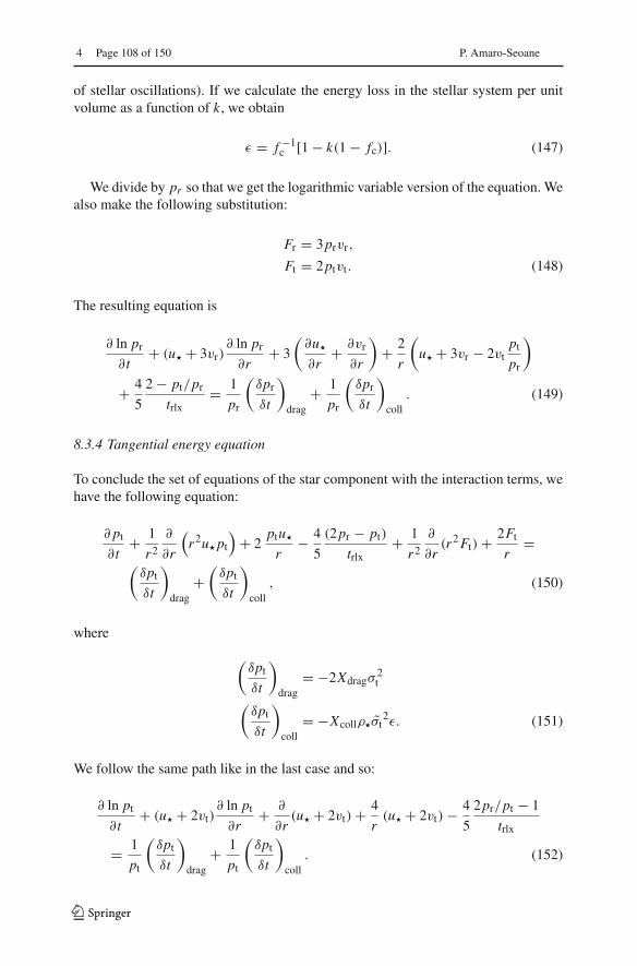
4 Page 108 of 150 P. Amaro-Seoane
of stellar oscillations). If we calculate the energy loss in the stellar system per unitvolume as a function of k, we obtain
ε = f −1c [1 − k(1 − fc)]. (147)
We divide by pr so that we get the logarithmic variable version of the equation. Wealso make the following substitution:
Fr = 3prvr,
Ft = 2ptvt. (148)
The resulting equation is
∂ ln pr
∂t+ (u� + 3vr)
∂ ln pr
∂r+ 3
(∂u�
∂r+ ∂vr
∂r
)+ 2
r
(u� + 3vr − 2vt
pt
pr
)
+ 4
5
2 − pt/pr
trlx= 1
pr
(δpr
δt
)drag
+ 1
pr
(δpr
δt
)coll
. (149)
8.3.4 Tangential energy equation
To conclude the set of equations of the star component with the interaction terms, wehave the following equation:
∂ pt
∂t+ 1
r2
∂
∂r
(r2u� pt
)+ 2
ptu�
r− 4
5
(2pr − pt)
trlx+ 1
r2
∂
∂r(r2Ft) + 2Ft
r=
(δpt
δt
)drag
+(
δpt
δt
)coll
, (150)
where
(δpt
δt
)drag
= −2Xdragσ2t
(δpt
δt
)coll
= −Xcollρ�σt2ε. (151)
We follow the same path like in the last case and so:
∂ ln pt
∂t+ (u� + 2vt)
∂ ln pt
∂r+ ∂
∂r(u� + 2vt) + 4
r(u� + 2vt) − 4
5
2pr/pt − 1
trlx
= 1
pt
(δpt
δt
)drag
+ 1
pt
(δpt
δt
)coll
. (152)
123

Relativistic dynamics and extreme mass ratio inspirals Page 109 of 150 4
8.4 Solving conducting, self-gravitating gas spheres
In this subsection, I explain briefly how the gaseous model is solved. The algorithmused is a partially implicit Newton–Raphson–Henyey iterative scheme, see Henyeyet al. (1959), Kippenhahn and Weigert (1994), their Sect. 11.2.
Putting aside the bounding conditions, the set of equations to be solved are Eq. (127)to (130). In practice, however, the equations are rewritten using the logarithm of allpositive quantities as dependant functions. As explained in Giersz and Spurzem (1994),this greatly improves energy conservation. Formally, one may write this system asfollows
∂x (i)
∂t+ f (i)
⎛⎝{x ( j),
∂x ( j)
∂r
}Neq
j=1
⎞⎠ = 0, for i = 1 . . . 4
f (i)
⎛⎝{x ( j),
∂x ( j)
∂r
}Neq
j=1
⎞⎠ = 0, for i = 5 . . . Neq, (153)
where the x (i) are the local quantities defining the state of the cluster, i.e.,
x ≡{x (1), x (2), . . . ox (Neq)
}≡ {log ρ, u, log pr, log p t, log Mr, vr − u, vt − u},
(154)with Neq = 7 in the present application.
To be solved numerically, this set of coupled partial differential equations have tobe discretized according to time and radius. Let us first consider time stepping. Let Δtbe the time step. Assume we know the solution x(t − Δt) at time t − Δt and want tocompute x(t). For the sake of numerical stability, a partially implicit scheme is used. Iadopt the shorthand notations x (i) ≡ x (i)(t) and y(i) ≡ x (i)(t − Δt). Time derivationis replaced by finite differences,
∂x (i)
∂t→ Δt−1(x (i) − y(i)). (155)
In the terms f (i), I replace the x ( j) by x ( j) which are intermediate values between y( j)
and x ( j), x ( j) = ζ x ( j) + (1 − ζ )y( j), with ζ = 0.55 for stability purposes (Giersz andSpurzem 1994).
Spatial discretisation is done by defining all quantities (at a given time) on a radialmesh, {r1, r2, . . . orNr } with r1 = 0 and rNr = rmax. A staggered mesh is implemented.While values of r , u, vt , vr and Mr are defined at the boundaries of the mesh cells,ρ, pt and pr are defined at the centre of each cell. When the value of a “boundary”quantity is needed at the centre of a cell, or vice-versa, one does a simple averaging,i.e., bk = (bk−1 + bk)/2, ck = (ck + ck+1)/2. Let us adopt the notation x ( j)
k for thevalue of x ( j) at position rk (or rk) and Δrk ≡ rk − rk−1. Then, radial derivatives inthe terms f (i) are approximated by finite differences,
123

4 Page 110 of 150 P. Amaro-Seoane
∂x ( j)
∂r→ x ( j)
k − x ( j)k−1
Δrk, (156)
if the derivative has to be evaluated at a point where xk is defined (centre or border ofa cell), or
∂x ( j)
∂r→
ˆx ( j)k − ˆx ( j)
k−1
Δrk= x ( j)
k+1 − x ( j)k−1
2Δrk, (157)
otherwise. As an exception, I use upstream differencing in ∂u/∂r for the secondequation in Eq. (127), i.e., the difference quotient is displaced by half a mesh pointupstream to improve stability.
By making the substitutions for ∂x ( j)/∂t and ∂x ( j)/∂r in the set of differentialequations (153), one obtains, at each mesh point rk , a set of Neq non-linear algebraicequations linking the new values to be determined, xk−1 and xk , to the “old” ones,yk−1
and yk, which are known,
F (i)k
(xk−1, xk |yk−1
, yk
)= 0
i = 1 . . . Neq, k = 1 . . . Nr.(158)
Note that the structure of the equations is the same at all mesh points, except fork = 1 and k = Nr. In particular, terms with index k − 1 do not appear in F (i)
1 . Also,one has to keep in mind that only the xk−1 and xk are unknown; the y
k−1and y
kplay the role of fixed parameters in these equations (as do the Δrk). If one defines a(Neq × Nr)-dimension vector X ∗ whose component Neq(k − 1) + i is x (i)
k , one canwrite the system of Neq × Nr equations as F ∗(X ∗) = 0, i.e.
F ∗(X ∗) ≡
⎛⎜⎜⎜⎜⎜⎜⎜⎜⎜⎜⎜⎜⎜⎜⎜⎜⎜⎜⎜⎜⎜⎜⎜⎝
F (1)1
F (2)1...
F(Neq)
1
F (1)2...
F(Neq)
2...
F (1)Nr...
F(Neq)
Nr
⎞⎟⎟⎟⎟⎟⎟⎟⎟⎟⎟⎟⎟⎟⎟⎟⎟⎟⎟⎟⎟⎟⎟⎟⎠
=⎛⎜⎝
0...
0
⎞⎟⎠ , (159)
123

Relativistic dynamics and extreme mass ratio inspirals Page 111 of 150 4
where I have defined
X ∗ ≡
⎛⎜⎜⎜⎜⎜⎜⎜⎜⎜⎜⎜⎜⎜⎜⎜⎜⎜⎜⎜⎜⎜⎜⎜⎝
x (1)1
x (2)1...
x(Neq)
1
x (1)2...
x(Neq)
2...
x (1)Nr...
x(Neq)
Nr
⎞⎟⎟⎟⎟⎟⎟⎟⎟⎟⎟⎟⎟⎟⎟⎟⎟⎟⎟⎟⎟⎟⎟⎟⎠
. (160)
The system is solved iteratively using a Newton–Raphson scheme. If X ∗[m] isthe approximation to the solution of Eq. (159) after iteration m, with F ∗[m] ≡F ∗(X ∗[m]) �= 0, the solution is refined through the relation
X ∗[m+1] = X ∗[m] −(
∂F ∗
∂X ∗
)−1
F ∗[m], (161)
where (∂F ∗/∂X ∗)−1 is the inverse of the matrix of derivatives. The latter, of dimen-sion (Neq Nr) × (Neq Nr), has the following structure
∂F ∗
∂X ∗ =
⎛⎜⎜⎜⎜⎜⎜⎜⎜⎜⎜⎜⎜⎝
� �+�− � �+
�− � �+. . .
. . .
�−k �k �+k. . .
. . .
�− � �+�− �
⎞⎟⎟⎟⎟⎟⎟⎟⎟⎟⎟⎟⎟⎠
. (162)
In this diagram, each square is a Neq × Neq sub-matrix. For 2 ≤ k ≤ Nr − 1, thelines Neqk − 6 to Neqk of ∂F ∗/∂X ∗ are composed of a group of 3 such Neq × Neqmatrices, �−k,�k,�+k that span columns Neqk − 13 to Neqk + Neq, while the restis composed of zeros,
123
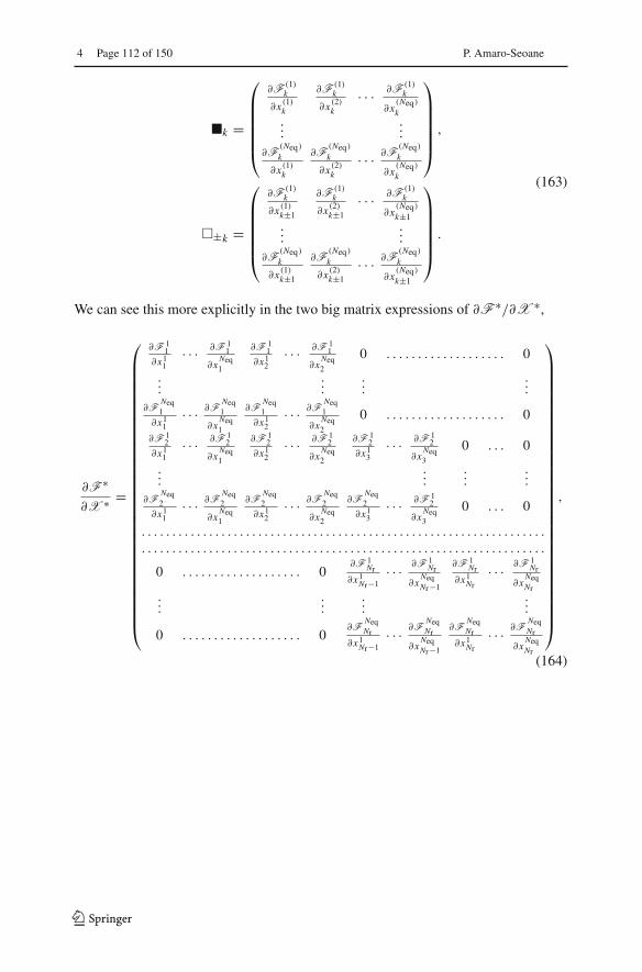
4 Page 112 of 150 P. Amaro-Seoane
�k =
⎛⎜⎜⎜⎜⎜⎝
∂F (1)k
∂x (1)k
∂F (1)k
∂x (2)k
· · · ∂F (1)k
∂x(Neq)
k...
...
∂F(Neq)
k
∂x (1)k
∂F(Neq)
k
∂x (2)k
· · · ∂F(Neq)
k
∂x(Neq)
k
⎞⎟⎟⎟⎟⎟⎠
,
�±k =
⎛⎜⎜⎜⎜⎜⎝
∂F (1)k
∂x (1)k±1
∂F (1)k
∂x (2)k±1
· · · ∂F (1)k
∂x(Neq)
k±1...
...
∂F(Neq)
k
∂x (1)k±1
∂F(Neq)
k
∂x (2)k±1
· · · ∂F(Neq)
k
∂x(Neq)
k±1
⎞⎟⎟⎟⎟⎟⎠
.
(163)
We can see this more explicitly in the two big matrix expressions of ∂F ∗/∂X ∗,
∂F ∗
∂X ∗ =
⎛⎜⎜⎜⎜⎜⎜⎜⎜⎜⎜⎜⎜⎜⎜⎜⎜⎜⎜⎜⎜⎜⎜⎜⎜⎜⎜⎜⎜⎜⎜⎜⎝
∂F 11
∂x11
· · · ∂F 11
∂xNeq1
∂F 11
∂x12
· · · ∂F 11
∂xNeq2
0 . . . . . . . . . . . . . . . . . . . 0
......
......
∂FNeq1
∂x11
· · · ∂FNeq1
∂xNeq1
∂FNeq1
∂x12
· · · ∂FNeq1
∂xNeq2
0 . . . . . . . . . . . . . . . . . . . 0
∂F 12
∂x11
· · · ∂F 12
∂xNeq1
∂F 12
∂x12
· · · ∂F 12
∂xNeq2
∂F 12
∂x13
· · · ∂F 12
∂xNeq3
0 . . . 0
......
......
∂FNeq2
∂x11
· · · ∂FNeq2
∂xNeq1
∂FNeq2
∂x12
· · · ∂FNeq2
∂xNeq2
∂FNeq2
∂x13
· · · ∂F 12
∂xNeq3
0 . . . 0
. . . . . . . . . . . . . . . . . . . . . . . . . . . . . . . . . . . . . . . . . . . . . . . . . . . . . . . . . . . . . . . . . .
. . . . . . . . . . . . . . . . . . . . . . . . . . . . . . . . . . . . . . . . . . . . . . . . . . . . . . . . . . . . . . . . . .
0 . . . . . . . . . . . . . . . . . . . 0∂F 1
Nr∂x1
Nr−1· · · ∂F 1
Nr
∂xNeqNr−1
∂F 1Nr
∂x1Nr
· · · ∂F 1Nr
∂xNeqNr
......
......
0 . . . . . . . . . . . . . . . . . . . 0∂F
NeqNr
∂x1Nr−1
· · · ∂FNeqNr
∂xNeqNr−1
∂FNeqNr
∂x1Nr
· · · ∂FNeqNr
∂xNeqNr
⎞⎟⎟⎟⎟⎟⎟⎟⎟⎟⎟⎟⎟⎟⎟⎟⎟⎟⎟⎟⎟⎟⎟⎟⎟⎟⎟⎟⎟⎟⎟⎟⎠
,
(164)
123

Relativistic dynamics and extreme mass ratio inspirals Page 113 of 150 4
The Heyney method is a way to take advantage of the special structure of the matrix∂F ∗/∂X ∗ to solve system (161) efficiently, with the number of operations scalinglike O(Nr) rather than O(N 3
r ) as would be the case if one uses a general-purposematrix inversion scheme.20 Setting B∗ ≡ −F ∗[m] and W ∗ ≡ X ∗[m+1] − X ∗[m],Eq. (161) is equivalent to (
∂F ∗
∂X ∗
)W ∗ = B∗, (165)
where W ∗ is the unknown vector. I further decompose vectors W ∗ and B∗ into Neq–dimensional sub-vectors, each one representing the values at a given mesh point,
W ∗ =
⎛⎜⎜⎜⎜⎜⎜⎜⎜⎝
W1W2...
Wk...
WNr
⎞⎟⎟⎟⎟⎟⎟⎟⎟⎠
. (166)
Then, the system (166) can be written as a set of coupled Neq–dimensional vectorequations,
�1W1 +�+1W2 =B1,
�−kWk−1 +�kWk +�+kWk+1=Bk,
�−NrWNr−1+�NrWNr =BNr .
(167)
The algorithm operates in two steps. First, going from k = 1 to Nr, one definesrecursively a sequence of Neq–vectors Vk and (Neq × Neq)–matrices Mk through
20 Memory usage is also reduced, scaling like O(Nr) rather than O(N2r ).
123
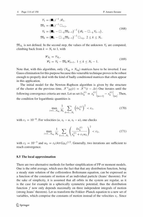
4 Page 114 of 150 P. Amaro-Seoane
V1 = (�1)−1 B1,
M1 = (�1)−1 �+1,
Vk = (�k − �−kMk−1
)−1 (Bk − �−kVk−1
),
Mk = (�k − �−kMk−1
)−1 �+k, 2 ≤ k ≤ Nr.
(168)
MNr is not defined. In the second step, the values of the unknown Vk are computed,climbing back from k = Nr to 1, with
WNr = VNr ,
Wk = Vk − MkWk+1, 1 ≤ k ≤ Nr − 1.(169)
Note that, with this algorithm, only (Neq × Neq) matrices have to be inverted. I useGauss elimination for this purpose because this venerable technique proves to be robustenough to properly deal with the kind of badly conditioned matrices that often appearin this application.
The initial model for the Newton–Raphson algorithm is given by the structureof the cluster at the previous time, X ∗[0](t) = X ∗(t − Δt) One iterates until the
following convergence criteria are met. Let us set δx (i)k ≡ x (i)
k
∣∣∣[m+1] − x (i)k
∣∣∣[m]. Then,
the condition for logarithmic quantities is
maxi=1...Neq
1
Nr
∑k=1...Nr
(δx (i)
k
)2< ε1, (170)
with ε1 = 10−6. For velocities (u, vr − u, vt − u), one checks
maxi=1...Neq
1
Nr
∑k=1...Nr
(δx (i)
k
x (i)k + ε1wk
)2
< ε2, (171)
with ε2 = 10−3 and wk = rk(4πGρk)1/2. Generally, two iterations are sufficient to
reach convergence.
8.5 The local approximation
There are two alternative methods for further simplification of FP or moment models.One is the orbit average, which uses the fact that that any distribution function, beinga steady state solution of the collisionless Boltzmann equation, can be expressed asa function of the constants of motion of an individual particle (Jeans’ theorem). Forthe sake of simplicity, it is assumed that all orbits in the system are regular, as itis the case for example in a spherically symmetric potential; thus the distributionfunction f now only depends maximally on three independent integrals of motion(strong Jeans’ theorem). Let us transform the Fokker–Planck equation to a new set ofvariables, which comprise the constants of motion instead of the velocities vi . Since
123

Relativistic dynamics and extreme mass ratio inspirals Page 115 of 150 4
in a spherically symmetric system the distribution only depends on energy and themodulus of the angular momentum vector, the number of independent coordinates inthis example can be reduced from six to two, and all terms in the transformed equationcontaining derivatives of other variables than energy and angular momentum vanish(in particular those containing derivatives of the spatial coordinates xi ). Integrating theremaining parts of the Fokker–Planck equation over the spatial coordinates is calledorbit averaging, because in our present example (a spherical system) it would be anintegration over accessible coordinate space for a given energy and angular momentum(which is a spherical shell between rmin(E, J ) and rmax(E, J ), the minimum andmaximum radius for stars with energy E and angular momentum J ). Such volumeintegration is, since f does not depend anymore on xi carried over to the diffusioncoefficients D, which become orbit-averaged diffusion coefficients.
Orbit-averaged Fokker–Planck models effectively deal with the diffusion of orbitsaccording to the changes of their constants of motion, taking into account the potentialand the orbital structure of the system in a self-consistent way. However, they are notfree of any problems or approximations. They require checks and tests, for exampleby comparisons with other methods, like the one described in the following. We treatrelaxation like the addition of a big non-correlated number of two-body encounters.Close encounters are rare and, thus, I suppose that each encounter produces a verysmall deflection angle. Thence, relaxation can be regarded as a diffusion process.21
A typical two-body encounter in a large stellar system takes place in a volumewhose linear dimensions are small compared to other typical radii of the system (totalsystem dimension, or scaling radii of changes in density or velocity dispersion). Con-sequently, it is assumed that an encounter only changes the velocity, not the positionof a particle. Thenceforth, encounters do not produce any changes Δx, so all relatedterms in the Fokker–Planck equation vanish. However, the local approximation goeseven further and assumes that the entire cumulative effect of all encounters on a testparticle can approximately be calculated as if the particle were surrounded by a verybig homogeneous system with the local distribution function (density, velocity dis-persions) everywhere. We are left with a Fokker–Planck equation containing onlyderivatives with respect to the velocity variables, but still depending on the spatialcoordinates (a local Fokker–Planck equation).
In practical astrophysical applications, the diffusion coefficients occurring in theFokker–Planck equation are not directly calculated, containing the probability Ψ fora velocity change Δv from an initial velocity v. Since D(Δvi ), and D(ΔviΔv j ) havedimensions of velocity (change) per time unit, and squared velocity (change) pertime unit, respectively, one calculates such velocity changes in a more direct way,considering a test star moving in a homogeneous sea of field stars. Let the test starhave a velocity v and consider an encounter with a field star of velocity v f . The resultof the encounter (i.e., velocity changes Δvi of the test star) is completely determinedby the impact parameter p and the relative velocity at infinity vrel = |v − v f |; thus byan integration of the type
21 Anyhow, it has been argued that rare deflections with a large angle may play a important role in thevicinity of a BH (Lin and Tremaine 1980).
123

4 Page 116 of 150 P. Amaro-Seoane
〈Δvi 〉p = 2π
∫(Δvi ) vrel n f p dp, (172)
the rate of change of the test star velocity due to encounters with vrel, in the field of starswith particle density n f , averaged over all relevant impact parameters is computed.The integration is normally carried out from p0 (impact parameter for 90◦ deflection)until R, which is some maximum linear dimension of the system under consideration.Such integration generates in subsequent equations the Coulomb logarithm ln Λ; aswe have seen previously, it can be well approximated by ln(0.11N ), where N is thetotal particle number. The diffusion coefficient finally is
D(Δvi ) =∫
〈Δvi 〉p f (v f )d3 v f , (173)
where f (v f ) is the velocity distribution of the field stars. In an equal mass system,f (v f ) should be equal to the distribution function of the test stars occurring in theFokker–Planck equation for self-consistency. In the case of a multi-mass system, how-ever, f (v f ) could be different from the test-star distribution, if the diffusion coefficientarising from encounters between two different species of stars is to be calculated. Thediffusion coefficients are (for an exact procedure see Binney and Tremaine 2008):
D(Δvi ) =4πG2m f ln Λ∂
∂vih(v),
D(Δviv j ) =4πG2m f ln Λ∂2
∂vi∂v jg(v), (174)
where h(v) and g(v) are given by the Rosenbluth potentials (Rosenbluth et al. 1957),
h(v) = (m + m f )
∫f (v f )
|v − v f |d3v f ,
g(v) = m f
∫f (v f )|v − v f |d3v f . (175)
With these results we can finally write down the local Fokker–Planck equation inits standard form for the Cartesian coordinate system of the vi :
(δ f
δt
)enc
= −4πG2m f ln Λ
[ 3∑i=1
∂
∂vi
(f (v)
∂h
∂vi
)+ 1
2
3∑i, j=1
∂2
∂vi∂v j
(f (v)
∂2g
∂vi∂v j
)]
(176)Note that in Rosenbluth et al. (1957), the above equation is given in a covari-
ant notation, which allows for a straightforward transformation into other curvilinearcoordinate systems.
Before going ahead the question is raised, why such approximation can be rea-sonable, regarding the long-range gravitational force, and the impossibility to shieldgravitational forces as in the case of Coulomb forces in a plasma by opposite charges.
123

Relativistic dynamics and extreme mass ratio inspirals Page 117 of 150 4
The key is that logarithmic intervals in impact parameter p contribute equally to themean square velocity change of a test particle, provided p � p0 (see, e.g., Spitzer Jr1987, Sect. 2.1). On one side, the lower limit of impact parameters (p0, the 90o deflec-tion angle impact parameter) is small compared to the mean interparticle distanced but, on the other side, D is a typical radius connected with a change in density orvelocity dispersions (e.g., the scale height in a disc of a galaxy), and R is the maximumtotal dimension of the system.
Let us assume D = 100 d, and R = 100 D. In that case the volume of the sphericalshell with radius between D and R is 106 times larger than the volume of the shelldefined by the radii d and D. Nevertheless the contribution of both shells to diffusioncoefficients or the relaxation time is approximately equal. This is a heuristic illustrationof why the local approximation is not so bad; the reason is that there are a lot moreencounters with particles in the outer, larger shell, but the effect is exactly compensatedby the larger deflection angle for encounters happening with particles from the innershell. If we are in the core or in the plane of a galactic disc the density would fall offfurther out, so the actual error will be smaller than outlined in the above example. Bythe same reasoning one can see, however, that the local approximation for a particle ina low-density region, which suffers from relaxation by a nearby density concentration,is prone to failure.
These simple examples should illustrate that under certain conditions the localapproximation is a priori not bad. On the other hand, it is obvious from our previousarguments that, if we are interested in relaxation effects on particles in a low-densityenvironment, whose orbit occasionally passes distant, high-density regions, the localapproximation could be completely wrong. One might think here, for example, ofstars on radially elongated orbits in the halo of globular clusters or of stars, globularclusters, or other objects as massive black holes, on spherical orbits in the galactichalo, passing the galactic disc. In these situations an orbit-averaged treatment seemsmuch more appropriate.
8.6 Monte Carlo codes
The Monte Carlo (MC) numerical scheme is intermediate in realism and numericalefficiency between Fokker–Planck or moment/gas approaches, which are very fast butbased on a significantly idealised description of the stellar system, and direct N -bodycodes, which treat (Newtonian) gravity in an essentially assumption-free way but areextremely demanding in terms of computing time. The MC scheme was first introducedby Hénon to follow the relaxational evolution of globular clusters (Hénon 1971a, b;Hénon 1973; Hénon 1975). To my knowledge, there exist three independent codesin active development and use that are based on Hénon’s ideas. The first is the onewritten by M. Giersz (see Giersz 2006), which implements many of the developmentsfirst introduced by Stodołkiewicz (Stodołkiewicz 1982, 1986). The second code is theone written by K. Joshi (Cluster Monte Carlo, MCM), see Joshi et al. (2000), Joshiet al. (2001) and greatly improved and extended by A. Gürkan and J. Fregeau (see,e.g., Fregeau et al. 2003; Gürkan et al. 2004; Fregeau et al. 2005; Gürkan et al. 2006and Pattabiraman et al. 2013 describing the latest parallel version). Finally, M. Freitag
123

4 Page 118 of 150 P. Amaro-Seoane
developed an MC code specifically aimed at the study of galactic nuclei containing acentral MBH (Freitag and Benz 2001, 2002; Freitag et al. 2006b).22 The descriptionof the method given here is based on this particular implementation.
The MC technique assumes that the cluster is spherically symmetric23 and rep-resents it as a set of particles, each of which may be considered as a homogeneousspherical shell of stars sharing the same orbital and stellar properties. The number ofparticles may be lower than the number of stars in the simulated cluster but the numberof stars per particle has to be the same for each particle. Another important assumptionis that the system is always in dynamical equilibrium so that orbital time scales neednot be resolved and the natural time-step is a fraction of the relaxation (or collision)time. Instead of being determined by integration of its orbit, the position of a particle(i.e., the radius R of the shell) is picked up at random, with a probability density forR that reflects the time spent at that radius: dP/dR ∝ 1/Vr(R) where Vr is the radialvelocity. The Freitag scheme adopts time steps that are a small fraction f of the local
relaxation (or collision) time: δt (R) � fδt(t−1rlx + t−1
coll
)−1. Consequently the central
parts of the cluster, where evolution is faster, are updated much more frequently thanthe outer parts. At each step, a pair of neighbouring particles is selected randomly withprobability Pselec ∝ 1/δt (R). This ensures that a particle stays for an average timeδt (R) at R before being updated.
Relaxation is treated as a diffusive process, using the classical Chandrasekhar theoryon which FP codes are also based. The long-term effects on orbits of the departure ofthe gravitational field from a smooth stationary potential are assumed to arise froma large number of uncorrelated, small angle, hyperbolic 2-body encounters. If a starof mass M1 travels with relative velocity vrel through a homogeneous field of stars ofmass M2 with number density n for a time δt , then in the centre-of-mass referenceframe, its trajectory will be deflected by an angle θδt with average values
〈θδt 〉 = 0, and
〈θ2δt 〉 = 8π ln ΛG2n (M1 + M2)
2 δt, (177)
where G is the gravitational constant and ln Λ � 10 − 15 is the Coulomb logarithm.In the MC code, at each step, the velocities of the particles of the selected pair are
modified by a hyperbolic encounter with deflection angle θeff =√
〈θ2δt 〉. The particles
are then put at random positions on the slightly modified orbits. As a given particlewill be selected many times, at various positions on its orbit, the MC scheme willintegrate the effect of relaxation over the particle’s orbit and over all possible fieldparticles. Proper averaging is ensured if the time steps are sufficiently short for theorbit to be modified significantly only after a large number of effective encounters.The energy is trivially conserved to machine accuracy in such a scheme because the
22 http://astro-gr.org/monte-carlo-simulations-for-stellar-dynamics/.23 But see Vasiliev (2015), who has developed a MC code base on the Princeton approach. The codefeatures a scheme to deal with asphericity, with the limitation that it assumes isotropy of the population ofbackground stars, so that it cannot model a highly flattened system with significant rotation support.
123
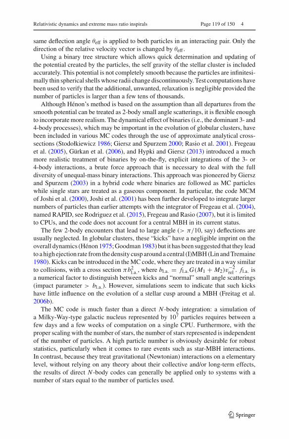
Relativistic dynamics and extreme mass ratio inspirals Page 119 of 150 4
same deflection angle θeff is applied to both particles in an interacting pair. Only thedirection of the relative velocity vector is changed by θeff .
Using a binary tree structure which allows quick determination and updating ofthe potential created by the particles, the self gravity of the stellar cluster is includedaccurately. This potential is not completely smooth because the particles are infinitesi-mally thin spherical shells whose radii change discontinuously. Test computations havebeen used to verify that the additional, unwanted, relaxation is negligible provided thenumber of particles is larger than a few tens of thousands.
Although Hénon’s method is based on the assumption than all departures from thesmooth potential can be treated as 2-body small angle scatterings, it is flexible enoughto incorporate more realism. The dynamical effect of binaries (i.e., the dominant 3- and4-body processes), which may be important in the evolution of globular clusters, havebeen included in various MC codes through the use of approximate analytical cross-sections (Stodołkiewicz 1986; Giersz and Spurzem 2000; Rasio et al. 2001). Fregeauet al. (2005), Gürkan et al. (2006), and Hypki and Giersz (2013) introduced a muchmore realistic treatment of binaries by on-the-fly, explicit integrations of the 3- or4-body interactions, a brute force approach that is necessary to deal with the fulldiversity of unequal-mass binary interactions. This approach was pioneered by Gierszand Spurzem (2003) in a hybrid code where binaries are followed as MC particleswhile single stars are treated as a gaseous component. In particular, the code MCMof Joshi et al. (2000), Joshi et al. (2001) has been further developed to integrate largernumbers of particles than earlier attempts with the integrator of Fregeau et al. (2004),named RAPID, see Rodriguez et al. (2015), Fregeau and Rasio (2007), but it is limitedto CPUs, and the code does not account for a central MBH in its current status.
The few 2-body encounters that lead to large angle (> π/10, say) deflections areusually neglected. In globular clusters, these “kicks” have a negligible imprint on theoverall dynamics (Hénon 1975; Goodman 1983) but it has been suggested that they leadto a high ejection rate from the density cusp around a central (I)MBH (Lin and Tremaine1980). Kicks can be introduced in the MC code, where they are treated in a way similarto collisions, with a cross section πb2
l.a., where bl.a. = fl.a.G(M1 + M2)v−2rel . fl.a. is
a numerical factor to distinguish between kicks and “normal” small angle scatterings(impact parameter > bl.a.). However, simulations seem to indicate that such kickshave little influence on the evolution of a stellar cusp around a MBH (Freitag et al.2006b).
The MC code is much faster than a direct N -body integration: a simulation ofa Milky-Way-type galactic nucleus represented by 107 particles requires between afew days and a few weeks of computation on a single CPU. Furthermore, with theproper scaling with the number of stars, the number of stars represented is independentof the number of particles. A high particle number is obviously desirable for robuststatistics, particularly when it comes to rare events such as star-MBH interactions.In contrast, because they treat gravitational (Newtonian) interactions on a elementarylevel, without relying on any theory about their collective and/or long-term effects,the results of direct N -body codes can generally be applied only to systems with anumber of stars equal to the number of particles used.
123

4 Page 120 of 150 P. Amaro-Seoane
8.7 Applications of Monte Carlo and Fokker–Planck simulations to the EMRIproblem
MC and FP codes are only appropriate for studying how collisional effects (principallyrelaxation) affect spherical systems in dynamical equilibrium. These assumptions areprobably valid within the radius of influence of MBHs with masses in the LISA range.Indeed, assuming naively that the Sgr A* cluster at the centre of our Galaxy is typical(as far as the total stellar mass and density is concerned) and that one can scale to othergalactic nuclei using the M−σ relation in the form σ = σMW(M•/3.6×106 M�)1/β
with β ≈ 4 − 5 (Ferrarese and Merritt 2000; Tremaine et al. 2002), one can estimatethe relaxation time at the radius of influence to be trlx(Rinfl) ≈ 25×109 yr (M•/3.6×106 M�)(2−3/β).
Although observations suggest a large spread amongst the values of the relaxationtime at the influence radius of MBHs with similar masses (see, e.g., Fig. 4 of Merrittet al. 2006), most galactic nuclei hosting MBHs less massive than a few 106 M� areprobably relaxed and amenable to MC or FP treatment. Even if the age of the system issignificantly smaller than its relaxation time, such approaches are valid as long as thenucleus is in dynamical equilibrium, with a smooth, spherical distribution of matter. Insuch conditions, relaxational processes are still controlling the EMRI rate, no matterhow long the relaxation time is, but one cannot assume a steady-state rate of diffusionof stars onto orbits with small periapsis, as is often done in FP codes (see the discussionin Milosavljevic and Merritt (2003), in the different context of the evolution of binaryMBHs).
The Hénon-type MC scheme of Freitag and Benz (2002) has been used to deter-mine the structure of galactic nuclei (Freitag and Benz 2002; Freitag et al. 2006b).Predictions for the distribution of stars around a MBH have also been obtained bysolving some form of the Fokker–Planck equation (Bahcall and Wolf 1977; Murphyet al. 1991; Hopman and Alexander 2006b, a; Merritt et al. 2006) or using the gaseousmodel (Amaro-Seoane 2004; Amaro-Seoane et al. 2004). These methods have proveduseful to determine how relaxation, collisions, large-angle scatterings, MBH growth,etc., shape the distribution of stars around the MBH, which is an obvious prerequisitefor the determination of the rate and characteristics of EMRIs. Of particular importanceis the inward segregation of stellar BHs as they lose energy to lighter objects. Thiseffect, combined with the fact that stellar BHs produce GWs with higher amplitudethan lower-mass stars, explains why they are expected to dominate the EMRI detectionrate (Sigurdsson and Rees 1997; Hopman and Alexander 2006a). An advantage of theMC approach is that it can easily and realistically include a continuous stellar massspectrum and extra physical ingredients. However, the first point might not be criticalhere as MC results suggest that, for models where all the stars were born ∼ 10 Gyrago, the pattern of mass segregation can be well approximated by a population of twocomponents only, one representing the stellar BHs and the other representing all other(lighter) objects (Freitag et al. 2006b). Furthermore, the uncertainties are certainlydominated by our lack of knowledge about where and when stellar formation takesplace in galactic nuclei, what the masses of the stars which form might be, and whattype of compact remnants they become.
123
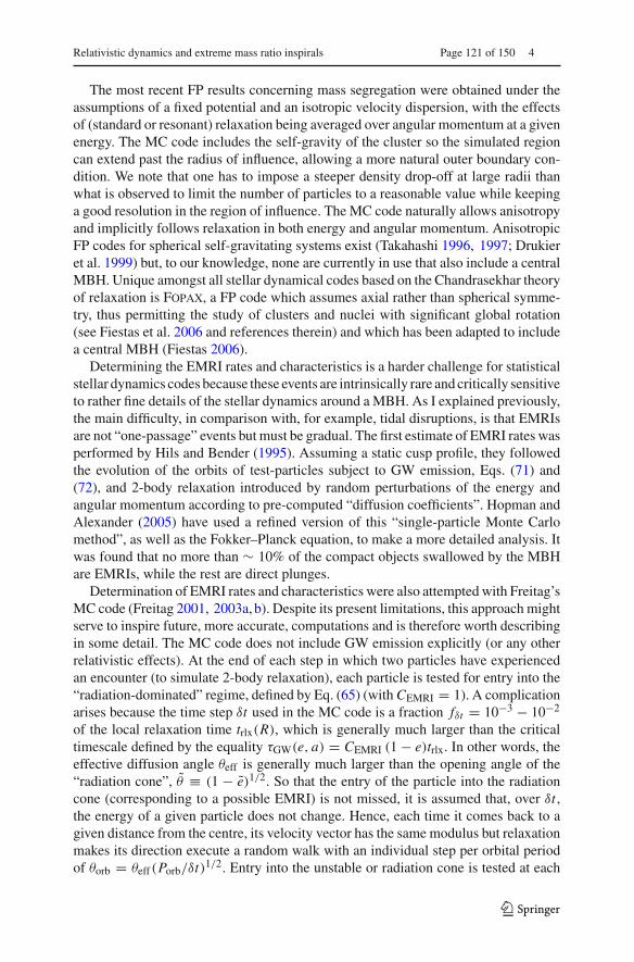
Relativistic dynamics and extreme mass ratio inspirals Page 121 of 150 4
The most recent FP results concerning mass segregation were obtained under theassumptions of a fixed potential and an isotropic velocity dispersion, with the effectsof (standard or resonant) relaxation being averaged over angular momentum at a givenenergy. The MC code includes the self-gravity of the cluster so the simulated regioncan extend past the radius of influence, allowing a more natural outer boundary con-dition. We note that one has to impose a steeper density drop-off at large radii thanwhat is observed to limit the number of particles to a reasonable value while keepinga good resolution in the region of influence. The MC code naturally allows anisotropyand implicitly follows relaxation in both energy and angular momentum. AnisotropicFP codes for spherical self-gravitating systems exist (Takahashi 1996, 1997; Drukieret al. 1999) but, to our knowledge, none are currently in use that also include a centralMBH. Unique amongst all stellar dynamical codes based on the Chandrasekhar theoryof relaxation is Fopax, a FP code which assumes axial rather than spherical symme-try, thus permitting the study of clusters and nuclei with significant global rotation(see Fiestas et al. 2006 and references therein) and which has been adapted to includea central MBH (Fiestas 2006).
Determining the EMRI rates and characteristics is a harder challenge for statisticalstellar dynamics codes because these events are intrinsically rare and critically sensitiveto rather fine details of the stellar dynamics around a MBH. As I explained previously,the main difficulty, in comparison with, for example, tidal disruptions, is that EMRIsare not “one-passage” events but must be gradual. The first estimate of EMRI rates wasperformed by Hils and Bender (1995). Assuming a static cusp profile, they followedthe evolution of the orbits of test-particles subject to GW emission, Eqs. (71) and(72), and 2-body relaxation introduced by random perturbations of the energy andangular momentum according to pre-computed “diffusion coefficients”. Hopman andAlexander (2005) have used a refined version of this “single-particle Monte Carlomethod”, as well as the Fokker–Planck equation, to make a more detailed analysis. Itwas found that no more than ∼ 10% of the compact objects swallowed by the MBHare EMRIs, while the rest are direct plunges.
Determination of EMRI rates and characteristics were also attempted with Freitag’sMC code (Freitag 2001, 2003a, b). Despite its present limitations, this approach mightserve to inspire future, more accurate, computations and is therefore worth describingin some detail. The MC code does not include GW emission explicitly (or any otherrelativistic effects). At the end of each step in which two particles have experiencedan encounter (to simulate 2-body relaxation), each particle is tested for entry into the“radiation-dominated” regime, defined by Eq. (65) (with CEMRI = 1). A complicationarises because the time step δt used in the MC code is a fraction fδt = 10−3 − 10−2
of the local relaxation time trlx(R), which is generally much larger than the criticaltimescale defined by the equality τGW(e, a) = CEMRI (1 − e)trlx. In other words, theeffective diffusion angle θeff is generally much larger than the opening angle of the“radiation cone”, θ ≡ (1 − e)1/2. So that the entry of the particle into the radiationcone (corresponding to a possible EMRI) is not missed, it is assumed that, over δt ,the energy of a given particle does not change. Hence, each time it comes back to agiven distance from the centre, its velocity vector has the same modulus but relaxationmakes its direction execute a random walk with an individual step per orbital periodof θorb = θeff(Porb/δt)1/2. Entry into the unstable or radiation cone is tested at each
123
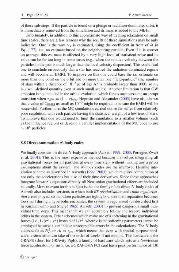
4 Page 122 of 150 P. Amaro-Seoane
of these sub-steps. If the particle is found on a plunge or radiation-dominated orbit, itis immediately removed from the simulation and its mass is added to the MBH.
Unfortunately, in addition to this approximate way of treating relaxation on smalltime scales, there are a few reasons why the results of these simulations may be onlyindicative. One is the way trlx is estimated, using the coefficient in front of δt inEq. (177), i.e., an estimate based on the neighbouring particle. Even if it is correcton average, this estimate is affected by a very high level of statistical noise and itsvalue can be far too long in some cases (e.g., when the relative velocity between theparticles in the pair is much larger than the local velocity dispersion). This could leadone to conclude erroneously that a star has reached the radiation-dominated regimeand will become an EMRI. To improve on this one could base the trlx estimate onmore than one point on the orbit and on more than one “field-particle” (the numberof stars within a distance of 10−2 pc of Sgr A* is probably larger than 1000, so trlxis a well-defined quantity even at such small scales). Another limitation is that GWemission is not included in the orbital evolution, which forces one to assume an abrupttransition when τGW = (1 − e)trlx. Hopman and Alexander (2005) have also shownthat a value of CEMRI as small as 10−3 might be required to be sure the EMRI will besuccessful. Furthermore, the MC simulations carried out so far suffer from relativelypoor resolution, with each particle having the statistical weight of a few tens of stars.To improve this one would need to limit the simulation to a smaller volume (suchas the influence region) or develop a parallel implementation of the MC code to use∼ 108 particles.
8.8 Direct-summation N-body codes
We finally consider the direct N -body approach (Aarseth 1999, 2003; Portegies Zwartet al. 2001). This is the most expensive method because it involves integrating allgravitational forces for all particles at every time step, without making any a prioriassumptions about the system. The N -body codes use the improved Hermite inte-gration scheme as described in Aarseth (1999, 2003), which requires computation ofnot only the accelerations but also of their time derivatives. Since these approachesintegrate Newton’s equations directly, all Newtonian gravitational effects are includednaturally. More relevant for this subject is that the family of the direct N -body codes ofAarseth also includes versions in which both KS regularisation and chain regularisa-tion are employed, so that when particles are tightly bound or their separation becomestoo small during a hyperbolic encounter, the system is regularised (as described firstin Kustaanheimo and Stiefel 1965; Aarseth 2003) to prevent dangerous small indi-vidual time steps. This means that we can accurately follow and resolve individualorbits in the system. Other schemes which make use of a softening in the gravitationalforces (i.e., 1/(r2 + ε2) instead of 1/r2, where ε is the softening parameter) cannot beemployed because ε can induce unacceptable errors in the calculations. The N -bodycodes scale as N 2
� , or Δt ∝ tdyn, which means that even with special-purpose hard-ware, a simulation can take of the order of weeks if not months. This hardware is theGRAPE (short for GRAvity PipE), a family of hardware which acts as a Newtonianforce accelerator. For instance, a GRAPE-6A PCI card has a peak performance of 130
123
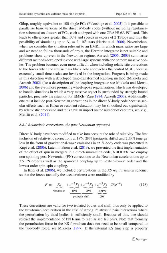
Relativistic dynamics and extreme mass ratio inspirals Page 123 of 150 4
Gflop, roughly equivalent to 100 single PCs (Fukushige et al. 2005). It is possible toparallelise basic versions of the direct N -body codes (without including regularisa-tion schemes) on clusters of PCs, each equipped with one GRAPE-6A PCI card. Thisleads to efficiencies greater than 50% and speeds in excess of 2 TFlops and thus thepossibility of simulating up to N� = 2 · 106 stars (Harfst et al. 2006). Nevertheless,when we consider the situation relevant to an EMRI, in which mass ratios are largeand we need to follow thousands of orbits, the Hermite integrator is not suitable andproblems show up even in the Newtonian regime. Aarseth (2006, 2003) summarisedifferent methods developed to cope with large systems with one or more massive bod-ies. The problem becomes even more difficult when including relativistic correctionsto the forces when the stellar-mass black hole approaches the central MBH, becauseextremely small time-scales are involved in the integration. Progress is being madein this direction with a developed time-transformed leapfrog method (Mikkola andAarseth 2002) (for a description of the leapfrog integrator see Mikkola and Merritt2006) and the even more promising wheel-spoke regularisation, which was developedto handle situations in which a very massive object is surrounded by strongly boundparticles, precisely the situation for EMRIs (Zare 1974; Aarseth 2003). Additionally,one must include post-Newtonian corrections in the direct N -body code because sec-ular effects such as Kozai or resonant relaxation may be smoothed out significantlyby relativistic precession and thus have an impact on the number of captures, see, e.g.,Merritt et al. (2011).
8.8.1 Relativistic corrections: the post-Newtonian approach
Direct N -body have been modified to take into account the role of relativity. The firstinclusion of relativistic corrections at 1PN, 2PN (periapsis shifts) and 2.5PN (energyloss in the form of gravitational-wave emission) in an N -body code was presented inKupi et al. (2006). Later, in Brem et al. (2013), we presented the first implementationof the effect of spin in mergers in a direct-summation code, NBODY6. We employnon-spinning post-Newtonian (PN) corrections to the Newtonian accelerations up to3.5 PN order as well as the spin-orbit coupling up to next-to-lowest order and thelowest order spin-spin coupling.
In Kupi et al. (2006), we included perturbations in the KS regularisation scheme,so that the forces (actually the accelerations) were modified by
F = F0︸︷︷︸Newtonian
+ c−2F2︸ ︷︷ ︸1PN
+ c−4F4︸ ︷︷ ︸2PN︸ ︷︷ ︸
periapsis shift
+ c−5F5︸ ︷︷ ︸2.5PN︸ ︷︷ ︸GW
+O(c−6) (178)
These corrections are valid for two isolated bodies and shall thus only be applied tothe Newtonian acceleration in the case of strong, relativistic pair-interactions wherethe perturbation by third bodies is sufficiently small. Because of this, one shouldrestrict the implementation of PN terms to regularised KS pairs. Note that formallythe perturbation force in the KS formalism does not need to be small compared tothe two-body force, see Mikkola (1997). If the internal KS time step is properly
123
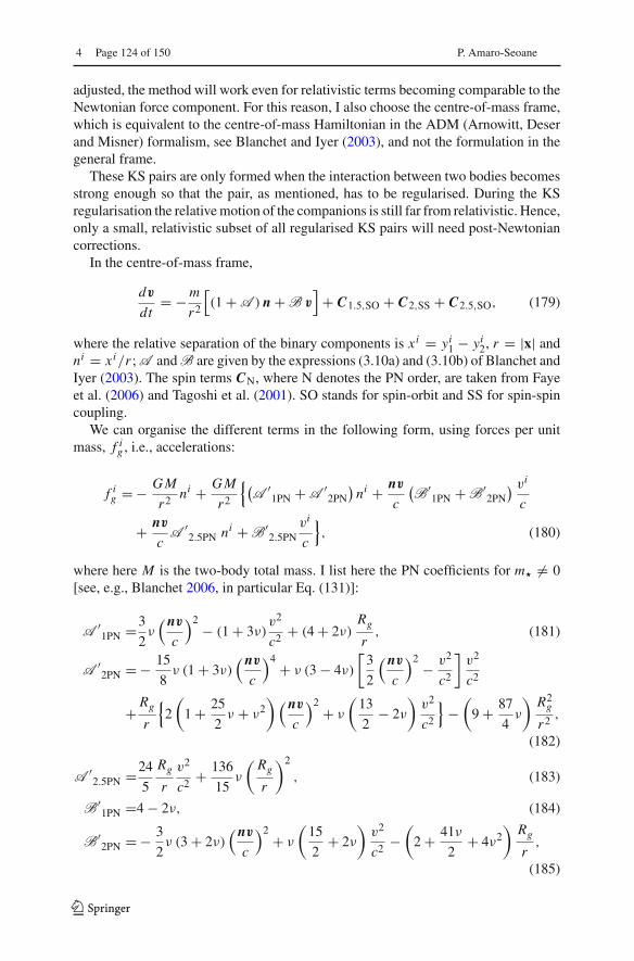
4 Page 124 of 150 P. Amaro-Seoane
adjusted, the method will work even for relativistic terms becoming comparable to theNewtonian force component. For this reason, I also choose the centre-of-mass frame,which is equivalent to the centre-of-mass Hamiltonian in the ADM (Arnowitt, Deserand Misner) formalism, see Blanchet and Iyer (2003), and not the formulation in thegeneral frame.
These KS pairs are only formed when the interaction between two bodies becomesstrong enough so that the pair, as mentioned, has to be regularised. During the KSregularisation the relative motion of the companions is still far from relativistic. Hence,only a small, relativistic subset of all regularised KS pairs will need post-Newtoniancorrections.
In the centre-of-mass frame,
dv
dt= −m
r2
[(1 + A ) n + B v
]+ C1.5,SO + C2,SS + C2.5,SO, (179)
where the relative separation of the binary components is xi = yi1 − yi2, r = |x| andni = xi/r ; A and B are given by the expressions (3.10a) and (3.10b) of Blanchet andIyer (2003). The spin terms CN, where N denotes the PN order, are taken from Fayeet al. (2006) and Tagoshi et al. (2001). SO stands for spin-orbit and SS for spin-spincoupling.
We can organise the different terms in the following form, using forces per unitmass, f ig , i.e., accelerations:
f ig = − GM
r2 ni + GM
r2
{(A ′
1PN + A ′2PN
)ni + nv
c
(B′
1PN + B′2PN
) vi
c
+ nv
cA ′
2.5PN ni + B′2.5PN
vi
c
}, (180)
where here M is the two-body total mass. I list here the PN coefficients for m� �= 0[see, e.g., Blanchet 2006, in particular Eq. (131)]:
A ′1PN =3
2ν(nv
c
)2 − (1 + 3ν)v2
c2 + (4 + 2ν)Rg
r, (181)
A ′2PN = − 15
8ν (1 + 3ν)
(nv
c
)4 + ν (3 − 4ν)
[3
2
(nv
c
)2 − v2
c2
]v2
c2
+ Rg
r
{2
(1 + 25
2ν + ν2
)(nv
c
)2 + ν
(13
2− 2ν
)v2
c2
}−(
9 + 87
4ν
)R2g
r2 ,
(182)
A ′2.5PN =24
5
Rg
r
v2
c2 + 136
15ν
(Rg
r
)2
, (183)
B′1PN =4 − 2ν, (184)
B′2PN = − 3
2ν (3 + 2ν)
(nv
c
)2 + ν
(15
2+ 2ν
)v2
c2 −(
2 + 41ν
2+ 4ν2
)Rg
r,
(185)
123
Relativistic dynamics and extreme mass ratio inspirals Page 125 of 150 4
B′2.5PN = − 24
5ν
(Rg
r
)2
− 8
5νRg
r
v2
c2 , (186)
where ν is the symmetric mass ratio, ν = m�M•/M2, with m� the mass of the stellar-mass black hole, and Rg = GM/c2. One can verify that the coefficients in Eqs. (228)to (231) agree with Eqs. (181) to (186) for ν = 0.
Whilst the gauge choice was not a problem for the system studied in Kupi et al.(2006), since we were interested in the global dynamical evolution, for the EMRIproblem the centre-of-mass frame (located at the origin of the coordinates) must beemployed. The integration cannot be extended to velocities higher than∼0.3 c, becauseat these velocities the post-Newtonian formalism can no longer be applied accurately.This means that we cannot reach the final coalescence of the stellar BH with theMBH, but this is not a big issue, because this part of the evolution does not contributesignificantly to the SNR of the GW signal. We note that it will not be possible to includein N -body codes all the PN corrections that are required for accurate modelling ofthe phase evolution of the EMRI during the last few years before plunge. However,the N -body codes are not required in that regime, since the system is then decoupledfrom the rest of the stellar cluster.
The expressions for the accelerations are:
a2 =Gm2
r2
{n[−v2
1 − 2v22 + 4v1v2 + 3
2(nv2)
2 + 5
(Gm1
r
)+ 4
(Gm2
r
)]
+ (v1 − v2) [4nv1 − 3nv2]
}(187)
a4 =Gm2
r2
{n[−2v4
2 + 4v22(v1v2) − 2(v1v2)
2 + 3
2v2
1(nv2)2 + 9
2v2
2(nv2)2
− 6(v1v2)(nv2)2 − 15
8(nv2)
4 +(Gm1
r
)
×(−15
4v2
1 + 5
4v2
2 − 5
2v1v2 + 39
2(nv1)
2 − 39(nv1)(nv2) + 17
2(nv2)
2)
+(Gm2
r
)(4v2
2 − 8v1v2 + 2(nv1)2 − 4(nv1)(nv2) − 6(nv2)
2)
]
+ (v1 − v2)
[v2
1(nv2) + 4v22(nv1) − 5v2
2(nv2) − 4(v1v2)(nv1) + 4(v1v2)(nv2)
− 6(nv1)(nv2)2 + 9
2(nv2)
3 +(Gm1
r
)(−63
4nv1 + 55
4nv2
)
+(Gm2
r
)(−2nv1 − 2nv2)
]}+ G3m2
r4 n[−57
4m2
1 − 9m22 − 69
2m1m2
],
(188)
a5 =4
5
G2m1m2
r3
{(v1 − v2)
[− (v1 − v2)
2 + 2
(Gm1
r
)− 8
(Gm2
r
)]
123
4 Page 126 of 150 P. Amaro-Seoane
+ n(nv1 − nv2)
[3(v1 − v2)
2 − 6
(Gm1
r
)+ 52
3
(Gm2
r
)]}. (189)
The basis of direct Nbody4 and Nbody6++ codes relies on an improved Hermitintegrator scheme by Makino and Aarseth (1992) and Aarseth (1999), for which weneed not only the accelerations but also their time derivative, given by
a0 = − Gm2
(v1 − v2
r3 + 3n
r3 (nv1 − nv2)
)(190)
a2 =Gm2{ −[(v1 − v2)
v21r3 + 2n
v1a1
r2 + 3nv2
1(nv2 − nv1)
r3
]
− 2
[(v1 − v2)
v22r3 + 2n
v2a2
r2 + 3nv2
2(nv2 − nv1)
r3
]
+ 4[(v1 − v2)
v1v2
r3 + na1v2 + a2v1
r2 + 3nv1v2(nv2 − nv1)
r3
]
+ 3
2
[(v1 − v2)
(nv2)2
r3 + 2n(nv2)r(na2) + v1v2 − v2
2r3
+ 5n(nv2)2(nv2 − nv1)
r3
]
+ G
[v1 − v2
r4 + 4nnv2 − nv1
r4
](5m1 + 4m2) + 4
nv1
r2 (a1 − a2)
+ 3nv2
r2 (a2 − a1)
+ 4v2
1 − v1v2 + r(na1) + 3(nv2 − nv1)nv1
r3 (v1 − v2)
+ 3v1v2 − v2
2 + r(na2) + 3(nv2 − nv1)nv2
r3 (v2 − v1) (191)
a4 =Gm2
{−2
[(v1 − v2)
v42r3 + n
4v22(a2v2)
r2 + 3nv4
2(nv2 − nv1)
r3
]
+ 4
[(v1 − v2)
v22v1v2
r3 + 2n(v2a2)(v1v2)
r2 + nv2
2(a1v2 + v1a2)
r2
+3nv2
2(v1v2)(nv2 − nv1)
r3
]
− 2
[(v1 − v2)
(v2v1)2
r3 + 2n(v1v2)(a1v2 + a2v1)
r2 + 3n(v1v2)2(nv2 − nv1)
r3
]
+ 3
2
[(v1 − v2)
v21(nv2)2
r3 + 2nv1a1(nv2)2
r2 + 2nv2
1(nv2)
r2
(na2 + v1v2 − v2
2r
)
+ 5nv2
1(nv2)2
r3 (nv2 − nv1)
]
123

Relativistic dynamics and extreme mass ratio inspirals Page 127 of 150 4
+ 9
2
[(v1 − v2)
v22(nv2)2
r3 + 2nv2a2(nv2)2
r2 + 2nv2
2(nv2)
r2
(na2 + v1v2 − v2
2r
)
+5nv2
2(nv2)2
r3 (nv2 − nv1)
]
− 6
[(v1 − v2)
v1v2(nv2)2
r3 + n(a1v2 + v1a2)(nv2)2
r2
+ 2nv1v2(nv2)
r2
(na2 + v1v2 − v2
2r
)+ 5n
v1v2(nv2)2(nv2 − nv1)
r3
]
− 15
8
[(v1 − v2)
(nv2)4
r3 + 4n(nv2)3
r2
(na2 + v1v2 − v2
2r
)
+7n(nv2)4
r3 (nv2 − nv1)
]
+ Gm1
⟨− 15
4
[(v1 − v2)
v21r4 + 2n
v1a1
r3 + 4nv2
1(nv2 − nv1)
r4
]
+ 5
4
[(v1 − v2)
v22r4 + 2n
v2a2
r3 + 4nv2
2(nv2 − nv1)
r4
]
− 5
2
[(v1 − v2)
v1v2
r4 + na1v2 + v1a2
r3 + 4nv1v2(nv2 − nv1)
r4
]
+ 39
2
[(v1 − v2)
(nv1)2
r4 + 2nnv1
r3
(na1 + v2
1 − v1v2
r
)
+ 6n(nv1)2(nv2 − nv1)
r4
]
− 39
[(v1 − v2)
(nv1)(nv2)
r4
+ n
r3
((nv1)(na2) + (nv2)(na1) + nv1(v1v2 − v2
2)
r+ nv2(v2
1 − v1v2)
r
)
+ 6n(nv1)(nv2)
r4 (nv2 − nv1)
]
+ 17
2
[(v1 − v2)
(nv2)2
r4 + 2nnv2
r3
(na2 + v1v2 − v2
2r
)
+6n(nv2)2(nv2 − nv1)
r4
] ⟩
+ Gm2
⟨4
[(v1 − v2)
v22r4 + 2n
v2a2
r3 + 4nv2
2(nv2 − nv1)
r4
]
− 8
[(v1 − v2)
v1v2
r4 + na1v2 + v1a2
r3 + 4nv1v2(nv2 − nv1)
r4
]
123

4 Page 128 of 150 P. Amaro-Seoane
+ 2
[(v1 − v2)
(nv1)2
r4 + 2nnv1
r3
{na1 + v2
1 − v1v2
r
}
+6n(nv1)2(nv2 − nv1)
r4
]
− 4
[(v1 − v2)
(nv1)(nv2)
r4
+ n
r3
{(nv1)(na2) + (nv2)(na1) + nv1(v1v2 − v2
2)
r+ nv2(v2
1 − v1v2)
r
}
+ 6n(nv1)(nv2)
r4 (nv2 − nv1)
]
− 6
[(v1 − v2)
(nv2)2
r4 + 2nnv2
r3
{na2 + v1v2 − v2
2r
}
+6n(nv2)2(nv2 − nv1)
r4
] ⟩
+ (a1 − a2)v2
1(nv2)
r2 + (v1 − v2)
×{
2(v1a1)(nv2)
r2 + v21r2
(na2 + v1v2 − v2
2r
+ 3nv2r
(nv2 − nv1)
)}
+ 4(a1 − a2)v2
2(nv1)
r2
+ 4(v1 − v2)
{2(v2a2)(nv1)
r2 + v22r2
(na1 + v2
1 − v1v2
r+ 3
nv1r
(nv2 − nv1)
)}
− 5(a1 − a2)v2
2(nv2)
r2
− 5(v1 − v2)
{2(v2a2)(nv2)
r2 + v22r2
(na2 + v1v2 − v2
2r
+ 3nv2r
(nv2 − nv1)
)}
− 4(a1 − a2)(v1v2)(nv1)
r2 − 4(v1 − v2)
{(a1v2 + v1a2)(nv1)
r2
+ v1v2
r2
(na1 + v2
1 − v1v2
r+ 3
(v1v2)(nv1)
r(nv2 − nv1)
)}
+ 4(a1 − a2)(v1v2)(nv2)
r2 + 4(v1 − v2)
{(a1v2 + v1a2)(nv2)
r2
+ v1v2
r2
(na2 + v1v2 − v2
2r
+ 3(v1v2)(nv2)
r(nv2 − nv1)
)}
− 6(a1 − a2)(nv1)(nv2)2
r2
− 6(v1 − v2)
{(nv2)2
r2
(na1 + v2
1 − v1v2
r
)
123

Relativistic dynamics and extreme mass ratio inspirals Page 129 of 150 4
+ 2(nv1)(nv2)
r2
(na2 + v1v2 − v2
2r
)+ 5
(nv1)(nv2)2
r3 (nv2 − nv1)
}
+ 9
2(a1 − a2)
(nv2)3
r2
+ 9
2(v1 − v2)
{3(nv2)2
r2
(na2 + v1v2 − v2
2r
)+ 5
(nv2)3
r3 (nv2 − nv1)
}
+ G
⟨[(a1 − a2)
nv1
r3 + (v1 − v2)
{na1
r3 + v21 − v1v2
r4 + 4nv1
r4 (nv2 − nv1)
}]
×[−63
4m1 − 2m2
]
+[(a1 − a2)
nv2
r3 + (v1 − v2)
{na2
r3 + v1v2 − v22
r4 + 4nv2
r4 (nv2 − nv1)
}]
×[
55
4m1 − 2m2
]⟩}
+ G3m2
(−57
4m2
1 − 9m22 − 69
2m1m2
)(v1 − v2
r5+ 5n
nv2 − nv1
r5
)(192)
a5 =4
5G2m1m2
{− (a1 − a2)(v1 − v2)2
r3 − 2v1 − v2
r3 (v1a1 + v2a2 − v2a1 − v1a2)
+ 6v1 − v2
r4 (v1 − v2)2(nv1 − nv2) + G(2m1 − 8m2)
×[a1 − a2
r4 + 4v1 − v2
r5(nv2 − nv1)
]
+ 3
[n
(v1 − v2)2
r3
(na1 − na2 + v2
1 + v22 − 2v1v2
r
)
+ 2nnv1 − nv2
r3 (v1a1 + v2a2 − v2a1 − v1a2)
− 5n(v1 − v2)2(nv1 − nv2)2
r4
]+ G
(52
3m2 − 6m1
)[(v1 − v2)
nv1 − nv2
r5
+ n
r4
(na1 − na2 + v2
1 − 2v1v2 + v22
r
)− 6n
(nv2 − nv1)2
r5
]}(193)
In the last expressions, I have used different kinds of brackets, including angle brackets forlegibility reasons. Gábor Kupi and I derived in 2005 independently the equations for our jointwork of Kupi et al. (2006) and compared the results with the output of a computer algebra systemby defining a function that was the substraction of our derivations and the numerical output.The result turned out to be smaller than 10−18. On the other hand, the terms have been nowtested by a number of independent works that adapted them in their codes. Also, in Brem et al.(2013) we did a series of tests that compared the terms with the semi-Keplerian approximationof Peters (1964).
In addition to the effects on the acceleration, the spin of compact objects of Eq. (179)undergoes precession in relativistic two-body interactions. This is also taken into account byintegrating the spin precession equations
123
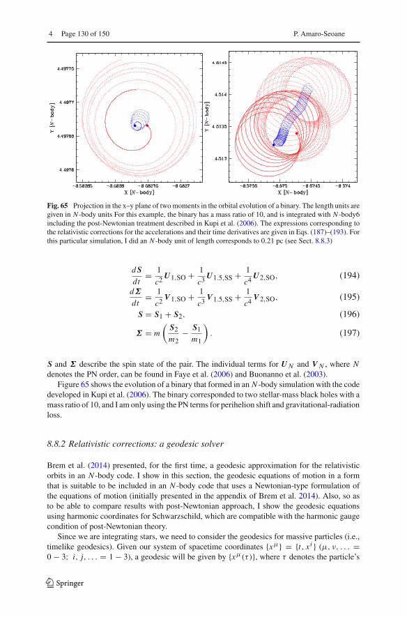
4 Page 130 of 150 P. Amaro-Seoane
Fig. 65 Projection in the x–y plane of two moments in the orbital evolution of a binary. The length units aregiven in N -body units For this example, the binary has a mass ratio of 10, and is integrated with N -body6including the post-Newtonian treatment described in Kupi et al. (2006). The expressions corresponding tothe relativistic corrections for the accelerations and their time derivatives are given in Eqs. (187)–(193). Forthis particular simulation, I did an N -body unit of length corresponds to 0.21 pc (see Sect. 8.8.3)
dSdt
= 1
c2 U1,SO + 1
c3 U1.5,SS + 1
c4 U2,SO, (194)
dΣ
dt= 1
c2 V1,SO + 1
c3 V1.5,SS + 1
c4 V2,SO, (195)
S = S1 + S2, (196)
Σ = m
(S2
m2− S1
m1
). (197)
S and Σ describe the spin state of the pair. The individual terms for UN and V N , where Ndenotes the PN order, can be found in Faye et al. (2006) and Buonanno et al. (2003).
Figure 65 shows the evolution of a binary that formed in an N -body simulation with the codedeveloped in Kupi et al. (2006). The binary corresponded to two stellar-mass black holes with amass ratio of 10, and I am only using the PN terms for perihelion shift and gravitational-radiationloss.
8.8.2 Relativistic corrections: a geodesic solver
Brem et al. (2014) presented, for the first time, a geodesic approximation for the relativisticorbits in an N -body code. I show in this section, the geodesic equations of motion in a formthat is suitable to be included in an N -body code that uses a Newtonian-type formulation ofthe equations of motion (initially presented in the appendix of Brem et al. 2014). Also, so asto be able to compare results with post-Newtonian approach, I show the geodesic equationsusing harmonic coordinates for Schwarzschild, which are compatible with the harmonic gaugecondition of post-Newtonian theory.
Since we are integrating stars, we need to consider the geodesics for massive particles (i.e.,timelike geodesics). Given our system of spacetime coordinates {xμ} = {t, xi } (μ, ν, . . . =0 − 3; i, j, . . . = 1 − 3), a geodesic will be given by {xμ(τ)}, where τ denotes the particle’s
123
Relativistic dynamics and extreme mass ratio inspirals Page 131 of 150 4
proper time. The components of the velocity vector are defined as
uμ = dxμ(τ)
dτ. (198)
This four-velocity vector satisfies:
gμνuμuν = −c2, (199)
where gμν is the Schwarzschild metric in our coordinate system and c denotes the speed of light.Since we are interested in geodesics, the velocity vector must satisfy the following equation ofmotion, see e.g., the book by Misner et al. (1973).
uν∇νuμ = 0, (200)
where ∇μ denotes the canonical covariant derivative associated with the spacetime metric gμν .Expanding this equation we have
duρ
dτ+ Γ
ρμνu
μuν = 0, (201)
being Γρμν the Christoffel symbols associated with the spacetime metric gμν . They are given in
terms of the metric by:
Γμαβ = 1
2gμν
(∂gαν
∂xβ+
∂gβν
∂xα−
∂gαβ
∂xρ
). (202)
Using the splitting of time and space we can write the velocity vector as follows:
u = ut∂
∂t+ ui
∂
∂xi, (203)
where {ut , ui } are the velocity components in the {t, xi } coordinate system:
ut = ∂t (τ )
∂τ, ui = ∂xi (τ )
∂τ. (204)
Therefore, on the trajectory of the particle we can write
ui = dxi (t)
dt
∂t
∂τ= vi ut ≡ Γ vi , (205)
where vi are the spatial components of the velocity
vi = dxi (t)
dt, (206)
123

4 Page 132 of 150 P. Amaro-Seoane
and Γ is the general relativistic version of the special relativistic gamma factor, which is givenin terms of the components of the spatial velocity and the metric tensor as:
Γ 2 = − c2
gtt + 2gtivi + gi jv
iv j. (207)
which, in the weak-field limit (gtt ≈ −c2 , gti ≈ 0 , gi j ≈ δi j ), has the usual expression:
Γ 2 ≈ 1
1 − v2
c2
, (v2 ≡ δi jviv j ). (208)
At this point, we can now adopt a Newtonian point of view by looking at the geodesicequations for the six quantities: {xi (t), vi (t)}, that is, for the spatial coordinates and spatialvelocity components. They can be written as:
dxi
dt= vi , (209)
dvi
dt= f ig, (210)
where, as we have mentioned before, the forces, f ig , are actually forces per unit mass, i.e.accelerations, since they should not depend on the mass of the body (according to the equiva-lence principle). Moreover, these specific forces depend on the spacetime metric (and its firstderivatives) and on vi . We can write them as
f ig = vi Γ tt t − Γ i
t t + 2(vi Γ t
t j − Γ it j
)v j +
(vi Γ t
jk − Γ ijk
)v jvk .
Given initial conditions {xio, vio}, Eqs. (209 and 210) have a unique solution {xi (t), vi (t)} .Note that the c2 factor dividing the forces, when going to the right-hand side of the equation(multiplying the Christoffel symbols) will cancel the c2 factor in the denominator of rg [seeexpressions in Eqs. (218)–(223)].
Since up to now, the development has been quite general, let us now consider the caseof a non-spinning (Schwarzschild) MBH black hole of mass M•. The metric components, inharmonic coordinates, can be written in the following form:
gtt = −1 − rgr
1 + rgr
c2, (211)
gti = 0, (212)
gi j = 1 + rgr
1 − rgr
ni n j +(
1 + rgr
)2 (δi j − ni n j
), (213)
where
r =√
δi j xi x j , ni = xi
r, rg = GM•
c2 . (214)
123

Relativistic dynamics and extreme mass ratio inspirals Page 133 of 150 4
From here, the components of the inverse metric are:
gtt = −1 + rgr
1 − rgr
1
c2 , (215)
gti = 0, (216)
gi j = 1 − rgr
1 + rgr
ni n j + 1(1 + rg
r
)2
(δi j − ni n j
), (217)
where xi = δi j xj and ni = δi j n
j .To determine the forces we need to compute the Christoffel symbols. From their defini-
tion (202), we find the following result
Γ tt t =0, (218)
Γ tti = rg
r2
ni
1 −( rgr
)2 , (219)
Γ ti j =0, (220)
Γ it t = rg
r2
1 − rgr(
1 + rgr
)3 ni c2, (221)
Γ it j =0, (222)
Γ ijk = rg
r21
1 + rgr
[(1 + rg
r
)ni(δ jk − n j nk
)−
ni n j nk
1 − rgr
− 2n( j
(δik) − ni nk)
)]. (223)
And this determines completely the geodesic equations of motion in Eqs. (209) and (210).Finally, we can make a post-Newtonian expansion of the equations of motion. That is, an
expansion for rg/r � 1 , and v/c � 1 . In our case, the expression for the force simplifies to[see Eq. (8.8.2) and Eqs. (218)–(223)]:
f ig = −Γ it t + 2 vi Γ t
t jvj − Γ i
jkvjvk . (224)
Expanding this we get:
f ig = − rgc2
r2
[1 − 4
rgr
+ 9
(rgr
)2
− 16
(rgr
)3]ni + 2
rgc2
r2
[1 +
(rgr
)2](
n jvj
c
)vi
c
− rgc2
r2
{ni(δ jk − n j nk
)−[
1 +(rgr
)2]ni n j nk − 2
[1 − rg
r+(rgr
)2
−(rgr
)3]
n( j
(δik) − ni nk)
)}× v j
c
vk
c, (225)
where the first two rows correspond to the first two terms in Eq. (224). We have expanded inTaylor series the functions of rg/r up to order (rg/r)
4 . We can now collect the terms and we
123

4 Page 134 of 150 P. Amaro-Seoane
find the following expression, which is valid to order 2PN [see Eq. (180) below]:
f ig = −GM•r2 ni + GM•
r2
{(A1PN + A2PN
)ni + n · v
c
(B1PN + B2PN
) vi
c
}, (226)
where
n · v
c= xcr
dxdt
= 1
2cr
dx2
dt= 1
2cr
dr
dt= r
c,
v2 =v · v = δi jviv j , (227)
and
A1PN =4rgr
− v2
c2 , (228)
A2PN = − 9
(rgr
)2+ 2
(n · v
c
)2 rgr
, (229)
B1PN =4, (230)
B2PN = − 2rgr
. (231)
8.8.3 N-body units and conversion
In N -body simulations, we use the so-called N -body units, as defined in, e.g., the book by Heggieand Hut (2003), although they were introduced in Heggie and Mathieu (1986). In these units,the total mass of the system M and G are set to unity, M = G = 1. Hence, to convert length r ,mass m, time t and velocity v from N -body (“Nbody”) to physical units (“phys”), we need tomultiply them by a conversion factor “conv”:
rphys = rconv · rNbody
mphys = mconv · mNbody
tphys = tconv · tNbody
vphys = vconv · vNbody .
We usually fix rconv by deciding the size of the system, and mconv is fixed to the average massof a star in the system, so that
tconv =√
r3conv
G mconv
vconv =√G mconv
rconv.
Acknowledgements I first of all thank my children, Antón and Natalia, for being the nicest children in theworld, and for their daily present of smiles during the long preparation of this work, in spite of my spasticand even spasmodic changes of mood as the article progressed (or retrogressed).
123

Relativistic dynamics and extreme mass ratio inspirals Page 135 of 150 4
I am particularly thankful to one of my best and closest friends, and also one of the brightest minds inthis field, Tal Alexander. Tal has given to me not just the present of his friendship, humour, company andcountless hours of smiles and laugh, which have made my life more beautiful, but also his wit and sharpnessin virtually any subject we discussed, in science or any other intellectual topic. He is a reference to me ashuman being and scientist. Many of the ideas I had would have never happened if it had not been for mydiscussions with him.It is a pleasure for me to show my most sincere gratitude to Francine Leeuwin and Marc Dewi Freitag. Themany discussions contributed enormously to the writing up of this review. More importantly, they “also”contributed enormously to my human formation during my freshman years of PhD student in Heidelberg. Iam also thankful to Bernard Schutz, Carlos F. Sopuerta, Xian Chen, Steve Drasco, Rainer Spurzem, RainerSchödel, Simos Konstantinidis, Miguel Preto, and Cole Miller both for discussions and their friendship(and waveforms, in the case of Steve). I am indebted to Emily Davidson for her titanic work of checkingmy abhorrent English, but also to Emma Robinson, Jon Gair, Melissa and Taka Tanaka. Part of this workhas been finished at the Max Planck Institute for Gravitational Physics (Albert Einstein Institute), Potsdam,Germany.
Open Access This article is distributed under the terms of the Creative Commons Attribution 4.0 Interna-tional License (http://creativecommons.org/licenses/by/4.0/), which permits unrestricted use, distribution,and reproduction in any medium, provided you give appropriate credit to the original author(s) and thesource, provide a link to the Creative Commons license, and indicate if changes were made.
A Comment on the use of the Ancient Greek word barathron andbathron to refer to a black hole
In the literature related to the main subject of this review, I have now and again found theexpression peribathron to refer to the concept of periapsis. Some authors use it in the case inwhich one has a black hole instead of a simple star (for which we have periastron). In this lastsection, I will try to convince the reader (from the Latin cum vincere, i.e., win with her or himthe truth) that this is not correct. Nevertheless, if one has an uncontrollable urge to be pedantic,I would instead recommend the term apo- or peribarathron. In the next lines I explain why.
From the Dictionnaire grec français, A. Bailly. ed. Hachette, édition no44, p. 347 we canfind that
b£raϑron,ou; tÒ I trou profond, d’où: 1 abîme, gouffre, ARSTT. Probl. 26, 28; part. àAthènes, barathre, gouffre où l’on précipitait les condamnés (cf. à Sparte cai£daz, DT.7, 133; PLAT. Gorg. 516 e; AR. Nub. 1450 // 2 fig. ruine, perte, DÈM. 101, 1; d’où causede ruine ou de perte, “un vrai gouffre”, en parl. d’une femme, THÉOPH. (ATH. 587 f) //II ornement de femme, AR. fr. 309, 8 // III c. br£ϑu HDT. l. c. v. ce mot (R. *gwera-/gwre/o,24 cf. ”ebrwn, lat. uoro, etc.).
On p. 340, we have the definition of b£ϑron
b£ϑronou; tÒ surface servant de fondement, d’où: 1 base HDT. 1, 183; part. piédestald’une statue, HDT. 5, 85; ESCH. Pers. 811; XÉN. Eq. 1, 1 // 2 degré, marche, HDT. 7,23; SOPH. O. C. 1591; part. degré d’échelle, échelon, EUR. Ph. 1179; HDN. 4, 2, 9;fig. cindÝnoub£ϑra, EUR. Cycl. 352, les approches (litt. les degrés d’un danger)// 3banc, siège SOPH. O. R. 142; O. C. 101; PLAT. Prot. 315 c; DÉM. 313, 12, etc.; b£ϑron(�…cmz) SOPH. Ant. 854, le trône (de la Justice)// 4 en gén. fondement solide, d’où sol(d’une maison, SOPH. Aj. 860; d’un pays, SOPH. Aj. 135; Phil. 1000); ou fondations,
24 Unfortunately, I was unable to reproduce the Indo-European root with the appropriate diacritical marks,due to limitations of typography, so I have approximated it.
123
4 Page 136 of 150 P. Amaro-Seoane
assises (de la terre, SOPH. O. C. 1662; d’une ville, EUR. Suppl. 1198); fig. fondement,support, PD. O. 13, 6; ™nb£ϑroiz e„nai EUR. Tr. 47, être ferme sur de solides fondements;™c b£ϑron DH. 8, 1; LUC. de fond en comble (ba…nw-ϑron;baϑrÒz)
The Greek–English Lexicon by Liddell & Scott, gives similar definitions. The short versioncan be consulted at the website of the Perseus Project.
The barathron (as it has been transliterated, e.g., by García Gual in the Odyssey, is described asan abyss, the pit of Tartarus, even though the name itself has never been employed exclusively—there is no “Barathron” par excellence. Here are the oldest references to it in the Homeric texts(reproduced below). By the way, in the Epic and in the Ionic dialect of Herodotus, one finds notb£raϑron, but the dialect variety bšreϑron, as Bailly indicates.
Iliad 8, 14 (Zeus very angry)“Hear me,” said he, “gods and goddesses, that I may speak even as I am minded. Letnone of you neither goddess nor god try to cross me, but obey me every one of you thatI may bring this matter to an end. If I see anyone acting apart and helping either Trojansor Danaans, he shall be beaten inordinately ere he come back again to Olympus; or I willhurl him down into dark Tartarus far into the deepest pit under the earth, where the gatesare iron and the floor bronze, as far beneath Hades as heaven is high above the earth, thatyou may learn how much the mightiest I am among you.”
Odyssey 12, 94 (Spanish, by García Gual)La otra ruta se abre entre dos promontorios. La cima de uno de ellos se clava en el cieloanchuroso (…) Tenebrosa caverna se abre a mitad de su altura orientada a las sombrasde ocaso y del Érebo (…) Ni el más hábil arquero podría desde el fondo del barco con suflecha alcanzar la oquedad de la cueva en que Escila vive haciendo sentir desde allí susterribles aullidos (…) La mitad de su cuerpo se esconde en la cóncava gruta; las cabezas,empero, por fuera del báratro horrible van mirando hacie el pie de la escarpa y exploransu presa (…)
Regarding this dialect variation (bšreϑron), we should note that it has been attested in ashorter or contracted form through syncope: bšϑron. This is what may lead to the mistake ofusing “bathron” instead of the correct form “barathron”. No dictionary mentions a potentialform bšϑron with the appropriate meaning, which might have existed under the same rule asbšϑron, i.e., as syncope form of the Attic variant b£raϑron.
Chantraine, in his book La formation des noms en grec ancien, states that barathron is a wordwith religious meaning. This should have been formed from an Indo-European root meaning “todevour” plus the suffix -thron (-ϑron), which expresses an instrument, tool or place, much likethe suffixes -tron and -terion. Its meaning is therefore something akin to “place of devouring”,“instrument or means of devouring”, “tool of devouring”. English “devour” comes throughFrench from the Latin form voro, from the same Indo-European root.
Bathron, on the other hand, seems to be formed from the same root as the verb ba…nw,which expresses the action of walking, lean the feet on the floor or in general to do any kind ofmovement on the floor. To this root one must add the same suffix of before and, so, we have a“place, tool or instrument to lean on”.
In conclusion, I maintain the words “bathron” and “barathron” are are nearly antonyms.“Barathron” expresses what one needs to express in the context of a black hole; “bathron” canbe envisaged as the opposite. What’s more, and what’s worse, in modern Greek, a “bathron” isa cesspit.
The Barathron was in ancient Greece a cliff in Athens, below which lay an inaccessible orinvisible place, where criminals were thrown to their deaths. This is attested in the works of
123

Relativistic dynamics and extreme mass ratio inspirals Page 137 of 150 4
Aristophanes, Plato and Herodotus (7133), and compiled by Bailly. It is not clear whether thisBarathron was a common name or a proper noun, namely a specific cliff. One should look inthe “Clouds” of Aristophanes.
According to Bailly, a cliff similar to the Barathron of Athens existed with the name“kaiadas”. So we can choose: peribarathron or perikaiadas.
Nevertheless, I would suggest something different. If you do not fancy periapsis or apoapsis,you could always make up a new word based on a modern language, such as English. In thatcase, I would advocate for the very nice term my friend Dave J. Vanecek coined in an e-mailexchange: “periholion”, from the English word “hole”.
References
Aarseth SJ (1999) From NBODY1 to NBODY6: the growth of an industry. Publ Astron Soc Jpn 111:1333–1346. https://doi.org/10.1086/316455
Aarseth SJ (2003) Black hole binary dynamics. Astrophys Space Sci 285:367–372. https://doi.org/10.1023/A:1025492510715
Aarseth SJ (2006) n-body codes. In: Highlights of astronomy 14, Proceedings of the IAU, vol 14. CambridgeUniversity Press. https://doi.org/10.1017/S1743921307011210
Alexander T (2007) Stellar relaxation processes near the galactic massive black hole. ArXiv e-prints0708.0688
Alexander T, Hopman C (2003) Orbital inspiral into a massive black hole in a galactic center. Astrophys JLett 590:L29–L32. https://doi.org/10.1086/376672
Alexander T, Hopman C (2009) Strong mass segregation around a massive black hole. Astrophys J697:1861–1869. https://doi.org/10.1088/0004-637X/697/2/1861
Amaro-Seoane P (2004) Dynamics of dense gas-star systems. Black holes and their precursors. PhD thesis,Heidelberg University. http://www.ub.uni-heidelberg.de/archiv/4826
Amaro-Seoane P, Chen X (2014) The fragmenting past of the disk at the galactic center: the culpritfor the missing red giants. Astrophys J Lett 781:L18. https://doi.org/10.1088/2041-8205/781/1/L18.arXiv:1310.0458
Amaro-Seoane P, Freitag M (2006) Intermediate-mass black holes in colliding clusters: implications forlower frequency gravitational-wave astronomy. Astrophys J Lett 653:L53–L56. https://doi.org/10.1086/510405. arXiv:astro-ph/0610478
Amaro-Seoane P, Preto M (2011) The impact of realistic models of mass segregation on the event rate ofextreme-mass ratio inspirals and cusp re-growth. Class Quantum Grav 28:094017. https://doi.org/10.1088/0264-9381/28/9/094017. arXiv:1010.5781
Amaro-Seoane P, Spurzem R (2001) The loss-cone problem in dense nuclei. Mon Not R Astron Soc327:995–1003. https://doi.org/10.1046/j.1365-8711.2001.04799.x
Amaro-Seoane P, Freitag M, Spurzem R (2004) Accretion of stars on to a massive black hole: a realisticdiffusion model and numerical studies. Mon Not R Astron Soc 352:655–672. https://doi.org/10.1111/j.1365-2966.2004.07956.x. arXiv:astro-ph/0401163
Amaro-Seoane P, Gair JR, Freitag M, Miller MC, Mandel I, Cutler CJ, Babak S (2007) Inter-mediate and extreme mass-ratio inspirals—astrophysics, science applications and detectionusing LISA. Class Quantum Grav 24:R113–R170. https://doi.org/10.1088/0264-9381/24/17/R01.arXiv:astro-ph/0703495
Amaro-Seoane P, Barranco J, Bernal A, Rezzolla L (2010) Constraining scalar fields with stellar kinematicsand collisional dark matter. J Cosmol Astropart Phys 2010(11):002. https://doi.org/10.1088/1475-7516/2010/11/002. arXiv:1009.0019
Amaro-Seoane P, Aoudia S, Babak S, Binétruy P, Berti E, Bohe A, Caprini C, Colpi M, Cornish NJ, Danz-mann K, Dufaux JF, Gair J, Jennrich O, Jetzer P, Klein A, Lang RN, Lobo A, Littenberg T, McWilliamsST, Nelemans G, Petiteau A, Porter EK, Schutz BF, Sesana A, Stebbins R, Sumner T, Vallisneri M,Vitale S, Volonteri M, Ward H (2012a) Low-frequency gravitational-wave science with eLISA/NGO.Class Quantum Grav 29:124016. https://doi.org/10.1088/0264-9381/29/12/124016. arXiv:1202.0839
123
4 Page 138 of 150 P. Amaro-Seoane
Amaro-Seoane P, Brem P, Cuadra J, Armitage PJ (2012b) The butterfly effect in the extreme-massratio inspiral problem. Astrophys J Lett 744:L20. https://doi.org/10.1088/2041-8205/744/2/L20.arXiv:1108.5174
Amaro-Seoane P, Aoudia S, Babak S, Binétruy P, Berti E, Bohé A, Caprini C, Colpi M, Cornish NJ,Danzmann K, Dufaux JF, Gair J, Jennrich O, Jetzer P, Klein A, Lang RN, Lobo A, Littenberg T,McWilliams ST, Nelemans G, Petiteau A, Porter EK, Schutz BF, Sesana A, Stebbins R, SumnerT, Vallisneri M, Vitale S, Volonteri M, Ward H (2013a) eLISA: astrophysics and cosmology in themillihertz regime. GW Notes 6:4–110 arXiv:1201.3621
Amaro-Seoane P, Sopuerta CF, Freitag MD (2013b) The role of the supermassive black hole spin in theestimation of the EMRI event rate. Mon Not R Astron Soc 429:3155–3165. https://doi.org/10.1093/mnras/sts572. arXiv:1205.4713
Amaro-Seoane P, Audley H, Babak S, Baker J, Barausse E, Bender P, Berti E, Binétruy P, Born M, BortoluzziD, Camp J, Caprini C, Cardoso V, Colpi M, Conklin J, Cornish N, Cutler C, Danzmann K, Dolesi R,Ferraioli L, Ferroni V, Fitzsimons E, Gair J, Gesa Bote L, Giardini D, Gibert F, Grimani C, Halloin H,Heinzel G, Hertog T, Hewitson M, Holley-Bockelmann (2017) Laser interferometer space antenna.ArXiv e-prints . Submitted to ESA on January 13th in response to the call for missions for the L3 slotin the Cosmic Vision Programme. arXiv:1702.00786
Armano M, Audley H, Auger G, Baird JT, Bassan M, Binétruy P, Born M, Bortoluzzi D, Brandt N, CalenoM, Carbone L, Cavalleri A, Cesarini A, Ciani G, Congedo G, Cruise AM, Danzmann K, de Deus SilvaM, De Rosa R, Diaz-Aguiló M, Di Fiore L, Diepholz I, Dixon G, Dolesi R, Dunbar N, Ferraioli L,Ferroni V, Fichter W, Fitzsimons ED, Flatscher R, Freschi M, García Marín AF, García MarirrodrigaC, Gerndt R, Gesa L, Gibert F, Giardini D, Giusteri R, Guzmán F, Grado A, Grimani C, Grynagier A,Grzymisch J, Harrison I, Heinzel G, Hewitson M, Hollington D, Hoyland D, Hueller M, InchauspéH, Jennrich O, Jetzer P, Johann U, Johlander B, Karnesis N, Kaune B, Korsakova N, Killow CJ, LoboJA, Lloro I, Liu L, López-Zaragoza JP, Maarschalkerweerd R, Mance D, Martín V, Martin-Polo L,Martino J, Martin-Porqueras F, Madden S, Mateos I, McNamara PW, Mendes J, Mendes L, MonskyA, Nicolodi D, Nofrarias M, Paczkowski S, Perreur-Lloyd M, Petiteau A, Pivato P, Plagnol E, PratP, Ragnit U, Raïs B, Ramos-Castro J, Reiche J, Robertson DI, Rozemeijer H, Rivas F, Russano G,Sanjuán J, Sarra P, Schleicher A, Shaul D, Slutsky J, Sopuerta CF, Stanga R, Steier F, Sumner T, TexierD, Thorpe JI, Trenkel C, Tröbs M, Tu HB, Vetrugno D, Vitale S, Wand V, Wanner G, Ward H, WarrenC, Wass PJ, Wealthy D, Weber WJ, Wissel L, Wittchen A, Zambotti A, Zanoni C, Ziegler T, ZweifelP (2016) Sub-Femto-g free fall for space-based gravitational wave observatories: LISA Pathfinderresults. Phys Rev Lett 116:231101. https://doi.org/10.1103/PhysRevLett.116.231101
Armano M, Audley H, Baird J, Binétruy P, Born M, Bortoluzzi D, Castelli E, Cavalleri A, Cesarini A,Cruise AM, Danzmann K, de Deus Silva M, Diepholz I, Dixon G, Dolesi R, Ferraioli L, FerroniV, Fitzsimons ED, Freschi M, Gesa L, Gibert F, Giardini D, Giusteri R, Grimani C, Grzymisch J,Harrison I, Heinzel G, Hewitson M, Hollington D, Hoyland D, Hueller M, Inchauspé H, Jennrich O,Jetzer P, Karnesis N, Kaune B, Korsakova N, Killow CJ, Lobo JA, Lloro I, Liu L, López-Zaragoza JP,Maarschalkerweerd R, Mance D, Meshksar N, Martín V, Martin-Polo L, Martino J, Martin-PorquerasF, Mateos I, McNamara PW, Mendes J, Mendes L, Nofrarias M, Paczkowski S, Perreur-Lloyd M,Petiteau A, Pivato P, Plagnol E, Ramos-Castro J, Reiche J, Robertson DI, Rivas F, Russano G, SlutskyJ, Sopuerta CF, Sumner T, Texier D, Thorpe JI, Vetrugno D, Vitale S, Wanner G, Ward H, Wass PJ,Weber WJ, Wissel L, Wittchen A, Zweifel P (2018) Beyond the required LISA free-fall performance:new LISA Pathfinder results down to 20 μHz. Phys Rev Lett 120:061101. https://doi.org/10.1103/PhysRevLett.120.061101
Arons J, Kulsrud RM, Ostriker JP (1975) A multiple pulsar model for quasi-stellar objects and active galacticnuclei. Astrophys J 198:687–705. https://doi.org/10.1086/153647
Babak S, Baker JG, Benacquista MJ, Cornish NJ, Larson SL, Mandel I, McWilliams ST, Petiteau A, PorterEK, Robinson EL, Vallisneri M, Vecchio A, Adams M, Arnaud KA, Błaut A, Bridges M, Cohen M,Cutler C, Feroz F, Gair JR, Graff P, Hobson M, Shapiro Key J, Królak A, Lasenby A, Prix R, Shang Y,Trias M, Veitch J, Whelan JT (2010) The mock LISA data challenges: from challenge 3 to challenge 4.Class Quantum Grav 27:084009. https://doi.org/10.1088/0264-9381/27/8/084009. arXiv:0912.0548
Babak S, Gair J, Sesana A, Barausse E, Sopuerta CF, Berry CPL, Berti E, Amaro-Seoane P, Petiteau A,Klein A (2017) Science with the space-based interferometer LISA. V. Extreme mass-ratio inspirals.Phys Rev D 95:103012. https://doi.org/10.1103/PhysRevD.95.103012. arXiv:1703.09722
Bahcall JN, Wolf RA (1976) Star distribution around a massive black hole in a globular cluster. AstrophysJ 209:214–232. https://doi.org/10.1086/154711
123

Relativistic dynamics and extreme mass ratio inspirals Page 139 of 150 4
Bahcall JN, Wolf RA (1977) The star distribution around a massive black hole in a globular cluster. II.Unequal star masses. Astrophys J 216:883–907. https://doi.org/10.1086/155534
Bar-Or B, Alexander T (2014) The statistical mechanics of relativistic orbits around a massive black hole.Class Quantum Grav 31:244003. https://doi.org/10.1088/0264-9381/31/24/244003. arXiv:1404.0351
Barack L, Cutler C (2004) LISA capture sources: approximate waveforms, signal-to-noise ratios, andparameter estimation accuracy. Phys Rev D 69:082005. https://doi.org/10.1103/PhysRevD.69.082005.arXiv:gr-qc/0310125
Barausse E, Rezzolla L (2008) Influence of the hydrodynamic drag from an accretion torus on extrememass-ratio inspirals. Phys Rev D 77. https://doi.org/10.1103/PhysRevD.77.104027. arXiv:0711.4558
Barausse E, Rezzolla L, Petroff D, Ansorg M (2007) Gravitational waves from extreme mass ratio inspi-rals in nonpure Kerr spacetimes. Phys Rev D 75. https://doi.org/10.1103/PhysRevD.75.064026.arXiv:gr-qc/0612123
Barausse E, Cardoso V, Pani P (2014) Can environmental effects spoil precision gravitational-wave astro-physics? Phys Rev D 89:104059. https://doi.org/10.1103/PhysRevD.89.104059. arXiv:1404.7149
Bardeen JM (1970) Kerr metric black holes. Nature 226:64–65. https://doi.org/10.1038/226064a0Barnes J, Hut P (1986) A hierarchical O(N log N ) force-calculation algorithm. Nature 324:446–449. https://
doi.org/10.1038/324446a0Bartko H, Martins F, Trippe S, Fritz TK, Genzel R, Ott T, Eisenhauer F, Gillessen S, Paumard T, Alexander
T, Dodds-Eden K, Gerhard O, Levin Y, Mascetti L, Nayakshin S, Perets HB, Perrin G, Pfuhl O,Reid MJ, Rouan D, Zilka M, Sternberg A (2010) An extremely top-heavy initial mass function inthe galactic center stellar disks. Astrophys J 708:834–840. https://doi.org/10.1088/0004-637X/708/1/834. arXiv:0908.2177
Baumgardt H, Makino J, Ebisuzaki T (2004a) Massive black holes in star clusters. I. Equal-mass clusters.Astrophys J 613:1133–1142
Baumgardt H, Makino J, Ebisuzaki T (2004b) Massive black holes in star clusters. II. Realistic clustermodels. Astrophys J 613:1143–1156
Baumgardt H, Amaro-Seoane P, Schödel R (2018) The distribution of stars around the Milky Way’s blackhole. III. Comparison with simulations. Astron Astrophys 609:A28. https://doi.org/10.1051/0004-6361/201730462. arXiv:1701.03818
Begelman MC (2010) Evolution of supermassive stars as a pathway to black hole formation. Mon Not RAstron Soc 402:673–681. https://doi.org/10.1111/j.1365-2966.2009.15916.x. arXiv:0910.4398
Bender PL, Hils D (1997) Confusion noise level due to galactic and extragalactic binaries. Class QuantumGrav 14:1439–1444. https://doi.org/10.1088/0264-9381/14/6/008
Bender PL, Armitage PJ, Begelman MC, Pema R (2005a) Massive black hole formation and growth. Whitepaper submitted to the NASA SEU Roadmap Committee
Bender R, Kormendy J, Bower G, Green R, Thomas J, Danks AC, Gull T, Hutchings JB, Joseph CL, KaiserME, Lauer TR, Nelson CH, Richstone D, Weistrop D, Woodgate B (2005b) HST STIS spectroscopyof the triple nucleus of M31: two nested disks in Keplerian rotation around a supermassive black hole.Astrophys J 631:280–300. https://doi.org/10.1086/432434. arXiv:astro-ph/0509839
Berry CPL, Gair JR (2013) Observing the galaxy’s massive black hole with gravitational wave bursts. MonNot R Astron Soc 429:589–612. https://doi.org/10.1093/mnras/sts360. arXiv:1210.2778
Bettwieser E, Spurzem R (1986) Anisotropy in stellar dynamics. Astron Astrophys 161:102–112Binney J, Tremaine S (1987) Galactic dynamics. Princeton University Press, PrincetonBinney J, Tremaine S (2008) Galactic dynamics, 2nd edn. Princeton University Press, PrincetonBlanchet L (2009) Gravitational radiation from post-newtonian sources and inspiralling compact binaries.
Living Rev Relativ 9:4. https://doi.org/10.12942/lrr-2006-4Blanchet L, Iyer BR (2003) Third post-Newtonian dynamics of compact binaries: equations of motion in
the centre-of-mass frame. Class Quantum Grav 20:755–776. https://doi.org/10.1088/0264-9381/20/4/309. arXiv:gr-qc/0209089
Bregman M, Alexander T (2009) Accretion disk warping by resonant relaxation: the case of maserdisk NGC 4258. Astrophys J Lett 700:L192–L195. https://doi.org/10.1088/0004-637X/700/2/L192.arXiv:0903.2051
Brem P, Amaro-Seoane P, Spurzem R (2013) Relativistic mergers of compact binaries in clusters: thefingerprint of the spin. Mon Not R Astron Soc 434:2999–3007. https://doi.org/10.1093/mnras/stt1220.arXiv:1302.3135
123
4 Page 140 of 150 P. Amaro-Seoane
Brem P, Amaro-Seoane P, Sopuerta CF (2014) Blocking low-eccentricity EMRIs: a statistical direct-summation N -body study of the Schwarzschild barrier. Mon Not R Astron Soc 437:1259–1267.https://doi.org/10.1093/mnras/stt1948. arXiv:1211.5601
Brown WR, Geller MJ, Kenyon SJ, Bromley BC (2009) The anisotropic spatial distribution ofhypervelocity stars. Astrophys J Lett 690:L69–L71. https://doi.org/10.1088/0004-637X/690/1/L69.arXiv:0811.0612
Buchholz RM, Schödel R, Eckart A (2009) Composition of the galactic center star cluster. Populationanalysis from adaptive optics narrow band spectral energy distributions. Astron Astrophys 499:483–501. https://doi.org/10.1051/0004-6361/200811497. arXiv:0903.2135
Buonanno A, Chen Y, Vallisneri M (2003) Detecting gravitational waves from precessing binaries of spin-ning compact objects: adiabatic limit. Phys Rev D 67:104025. https://doi.org/10.1103/PhysRevD.67.104025. arXiv:gr-qc/0211087
Chabrier G, Baraffe I (2000) Theory of low-mass stars and substellar objects. Annu Rev Astron Astrophys38:337–377. https://doi.org/10.1146/annurev.astro.38.1.337. arXiv:astro-ph/0006383
Chandrasekhar S (1942) Principles of stellar dynamics. University of Chicago, ChicagoChandrasekhar S (1960) Principles of stellar dynamics, enlarged edn. Dover, Mineola, NYChang JS, Cooper G (1970) A practical difference scheme for Fokker–Planck equations. J Comput Phys
6:1–16. https://doi.org/10.1016/0021-9991(70)90001-XChen X, Amaro-Seoane P (2014) A rapidly evolving region in the galactic center: why S-stars thermalize
and more massive stars are missing. Astrophys J Lett 786:L14. https://doi.org/10.1088/2041-8205/786/2/L14. arXiv:1401.6456
Chen X, Sesana A, Madau P, Liu FK (2011) Tidal stellar disruptions by massive black hole pairs. II. Decayingbinaries. Astrophys J 729:13. https://doi.org/10.1088/0004-637X/729/1/13. arXiv:1012.4466
Chernoff DF, Weinberg MD (1990) Evolution of globular clusters in the galaxy. Astrophys J 351:121–156.https://doi.org/10.1086/168451
Clutton-Brock M (1973) The gravitational field of three dimensional galaxies. Astrophys Space Sci 23:55–69. https://doi.org/10.1007/BF00647652
Cohn H (1979) Numerical integration of the Fokker–Planck equation and the evolution of star clusters.Astrophys J 234:1036–1053. https://doi.org/10.1086/157587
Cohn H (1980) Late core collapse in star clusters and the gravothermal instability. Astrophys J 242:765–771.https://doi.org/10.1086/158511
Cohn H (1985) Direct Fokker–Planck calculations. In: Goodman J, Hut P (eds) Dynamics of star clusters.IAU Symposia, vol 113. D. Reidel, Dordrecht, pp 161–177
Cohn H, Kulsrud RM (1978) The stellar distribution around a black hole: numerical integration of theFokker–Planck equation. Astrophys J 226:1087–1108. https://doi.org/10.1086/156685
Collin S, Zahn JP (1999) Accretion disks and star formation. In: Terzian Y, Khachikian E, Weedman D(eds) Active galactic nuclei and related phenomena. IAU Symposia, vol 194. Astronomical Society ofthe Pacific, San Francisco, p 246
Cutler C, Harms J (2006) Big Bang Observer and the neutron-star-binary subtraction problem. Phys Rev D73:042001. https://doi.org/10.1103/PhysRevD.73.042001. arXiv:gr-qc/0511092
Cutler C, Kennefick D, Poisson E (1994) Gravitational radiation reaction for bound motion around aSchwarzschild black hole. Phys Rev D 50:3816–3835. https://doi.org/10.1103/PhysRevD.50.3816
Danzmann K (2000) LISA mission overview. Adv Space Res 25:1129–1136. https://doi.org/10.1016/S0273-1177(99)00973-4
David LP, Durisen RH, Cohn HN (1987a) The evolution of active galactic nuclei. I. Models without stellarevolution. Astrophys J 313:556–575
David LP, Durisen RH, Cohn HN (1987b) The evolution of active galactic nuclei. II. Models with stellarevolution. Astrophys J 316:505–516
Do T, Ghez AM, Morris MR, Lu JR, Matthews K, Yelda S, Larkin J (2009) High angular resolution integral-field spectroscopy of the Galaxy’s nuclear cluster: a missing stellar cusp? Astrophys J 703:1323–1337.https://doi.org/10.1088/0004-637X/703/2/1323. arXiv:0908.0311
Drukier GA, Cohn HN, Lugger PM, Yong H (1999) Anisotropic Fokker–Planck models for the evolutionof globular star clusters: the core-halo connection. Astrophys J 518:233–245. https://doi.org/10.1086/307243
Duncan MJ, Shapiro SL (1983) Monte Carlo simulations of the evolution of galactic nuclei containingmassive, central black holes. Astrophys J 268:565–581. https://doi.org/10.1086/160980
123

Relativistic dynamics and extreme mass ratio inspirals Page 141 of 150 4
Eilon E, Kupi G, Alexander T (2009) The efficiency of resonant relaxation around a massive black hole.Astrophys J 698:641–647. https://doi.org/10.1088/0004-637X/698/1/641. arXiv:0807.1430
eLISA Consortium, Amaro-Seoane P, Aoudia S, Audley H, Auger G, Babak S, Baker J, Barausse E, BarkeS, Bassan M, Beckmann V, Benacquista M, Bender PL, Berti E, Binétruy P, Bogenstahl J, Bonvin C,Bortoluzzi D, Brause NC, Brossard J, Buchman S, Bykov I, Camp J, Caprini C, Cavalleri A, CerdonioM, Ciani G, Colpi M, Congedo G, Conklin J, Cornish N, Danzmann K, de Vine G, DeBra D, DewiFreitag M, Di Fiore L, Diaz Aguilo M, Diepholz I, Dolesi R, Dotti M, Fernández Barranco G, FerraioliL, Ferroni V, Finetti N, Fitzsimons E, Gair J, Galeazzi F, Garcia A, Gerberding O, Gesa L, Giardini D,Gibert F, Grimani C, Groot P, Guzman Cervantes F, Haiman Z, Halloin H, Heinzel G, Hewitson M,Hogan C, Holz D, Hornstrup A, Hoyland D, Hoyle CD, Hueller M, Hughes S, Jetzer P, Kalogera V,Karnesis N, Kilic M, Killow C, Klipstein W, Kochkina E, Korsakova N, Krolak A, Larson S, Lieser M,Littenberg T, Livas J, Lloro I, Mance D, Madau P, Maghami P, Mahrdt C, Marsh T, Mateos I, Mayer L,McClelland D, McKenzie K, McWilliams S, Merkowitz S, Miller C, Mitryk S, Moerschell J, MohantyS, Monsky A, Mueller G, Müller V, Nelemans G, Nicolodi D, Nissanke S, Nofrarias M, Numata K,Ohme F, Otto M, Perreur-Lloyd M, Petiteau A, Phinney ES, Plagnol E, Pollack S, Porter E, Prat P,Preston A, Prince T, Reiche J, Richstone D, Robertson D, Rossi EM, Rosswog S, Rubbo L, Ruiter A,Sanjuan J, Sathyaprakash BS, Schlamminger S, Schutz B, Schütze D, Sesana A, Shaddock D, Shah S,Sheard B, Sopuerta CF, Spector A, Spero R, Stanga R, Stebbins R, Stede G, Steier F, Sumner T, SunKX, Sutton A, Tanaka T, Tanner D, Thorpe I, Tröbs M, Tinto M, Tu HB, Vallisneri M, Vetrugno D,Vitale S, Volonteri M, Wand V, Wang Y, Wanner G, Ward H, Ware B, Wass P, Weber WJ, Yu Y, YunesN, Zweifel P (2013) The gravitational universe. ArXiv e-prints Submitted to ESA on May 24th, 2013for the L2/L3 selection of ESA’s Cosmic Vision program. arXiv:1305.5720
Elson R, Hut P, Inagaki S (1987) Dynamical evolution of globular clusters. Annu Rev Astron Astrophys25:565–601. https://doi.org/10.1146/annurev.aa.25.090187.003025
Faye G, Blanchet L, Buonanno A (2006) Higher-order spin effects in the dynamics of compact bina-ries. I. Equations of motion. Phys Rev D 74:104033. https://doi.org/10.1103/PhysRevD.74.104033.arXiv:gr-qc/0605139
Fellhauer M, Kroupa P, Baumgardt H, Bien R, Boily CM, Spurzem R, Wassmer N (2000) SUPERBOX—anefficient code for collisionless galactic dynamics. Nature 5:305–326. https://doi.org/10.1016/S1384-1076(00)00032-4. arXiv:astro-ph/0007226
Ferrarese L, Ford H (2005) Supermassive black holes in galactic nuclei: past, present and future research.Space Sci Rev 116:523–624. https://doi.org/10.1007/s11214-005-3947-6
Ferrarese L, Merritt D (2000) A fundamental relation between supermassive black holes and their hostgalaxies. Astrophys J Lett 539:L9–L12. https://doi.org/10.1086/312838
Ferrarese L, Pogge RW, Peterson BM, Merritt D, Wandel A, Joseph CL (2001) Supermassive black holesin active galactic nuclei. I. The consistency of black hole masses in quiescent and active galaxies.Astrophys J Lett 555:L79–L82. https://doi.org/10.1086/322528
Fiestas J (2006) Dynamical evolution of rotating globular clusters with embedded black holes. PhD thesis,Heidelberg University
Fiestas J, Spurzem R, Kim E (2006) 2D Fokker–Planck models of rotating clusters. Mon Not R Astron Soc373:677–686. https://doi.org/10.1111/j.1365-2966.2006.11036.x. arXiv:astro-ph/0609056
Finn LS (1992) Detection, measurement, and gravitational radiation. Phys Rev D 46:5236–5249. https://doi.org/10.1103/PhysRevD.46.5236. arXiv:gr-qc/9209010
Finn LS, Thorne KS (2000) Gravitational waves from a compact star in a circular, inspiral orbit, in theequatorial plane of a massive, spinning black hole, as observed by LISA. Phys Rev D 62:124021.https://doi.org/10.1103/PhysRevD.62.124021
Frank J, Rees MJ (1976) Effects of massive central black holes on dense stellar systems. Mon Not R AstronSoc 176:633–647. https://doi.org/10.1093/mnras/176.3.633
Fregeau JM, Rasio FA (2007) Monte Carlo simulations of globular cluster evolution. IV. Directintegration of strong interactions. Astrophys J 658:1047–1061. https://doi.org/10.1086/511809.arXiv:astro-ph/0608261
Fregeau JM, Gürkan MA, Joshi KJ, Rasio FA (2003) Monte Carlo simulations of globular cluster evolution.III. Primordial binary interactions. Astrophys J 593:772–787. https://doi.org/10.1086/376593
Fregeau JM, Cheung P, Portegies Zwart SF, Rasio FA (2004) Stellar collisions during binary–binary andbinary–single star interactions. Mon Not R Astron Soc 352:1–19. https://doi.org/10.1111/j.1365-2966.2004.07914.x. arXiv:astro-ph/0401004
123

4 Page 142 of 150 P. Amaro-Seoane
Fregeau JM, Gürkan MA, Rasio FA (2005) Star cluster evolution with primordial binaries. ArXiv e-printsastro-ph/0512032
Freitag M (2001) Monte Carlo cluster simulations to determine the rate of compact star inspiralling to acentral galactic black hole. Class Quantum Grav 18:4033–4038. https://doi.org/10.1088/0264-9381/18/19/309
Freitag M (2003a) Captures of stars by a massive black hole: investigations in numerical stellar dynamics.In: Centrella JM (ed) The astrophysics of gravitational wave sources, AIP conference proceedings,vol 686. American Institute of Physics, pp 109–112
Freitag M (2003b) Gravitational waves from stars orbiting the Sagittarius A* black hole. Astrophys J Lett583:L21–L24. https://doi.org/10.1086/367813. arXiv:astro-ph/0211209
Freitag M, Benz W (2001) A new Monte Carlo code for star cluster simulations: I. Relaxation. AstronAstrophys 375:711–738. https://doi.org/10.1051/0004-6361:20010706
Freitag M, Benz W (2002) A new Monte Carlo code for star cluster simulations: II. Central black hole andstellar collisions. Astron Astrophys 394:345–374. https://doi.org/10.1051/0004-6361:20021142
Freitag M, Benz W (2005) A comprehensive set of simulations of high-velocity collisions between main-sequence stars. Mon Not R Astron Soc 358:1133–1158. https://doi.org/10.1111/j.1365-2966.2005.08770.x. arXiv:astro-ph/0403621
Freitag M, Amaro-Seoane P, Kalogera V (2006a) Models of mass segregation at the galactic centre. J PhysConf Ser 54:252–258. https://doi.org/10.1088/1742-6596/54/1/040. arXiv:astro-ph/0607001
Freitag M, Amaro-Seoane P, Kalogera V (2006b) Stellar remnants in galactic nuclei: mass segregation.Astrophys J 649:91–117. https://doi.org/10.1086/506193. arXiv:astro-ph/0603280
de Freitas Pacheco JA, Filloux C, Regimbau T (2006) Capture rates of compact objects by supermassive blackholes. Phys Rev D 74:023001. https://doi.org/10.1103/PhysRevD.74.023001. arXiv:astro-ph/0606427
Fukushige T, Makino J, Kawai A (2005) GRAPE-6A: a single-card GRAPE-6 for parallel PC-GRAPE cluster systems. Publ Astron Soc Jpn 57:1009–1021. https://doi.org/10.1093/pasj/57.6.1009.arXiv:astro-ph/0504407
Gaburov E, Harfst S, Portegies Zwart S (2009) SAPPORO: a way to turn your graphics cards into a GRAPE-6. New Astron 14:630–637. https://doi.org/10.1016/j.newast.2009.03.002. arXiv:0902.4463
Gair JR (2009) Probing black holes at low redshift using LISA EMRI observations. Class Quantum Grav26:094034. https://doi.org/10.1088/0264-9381/26/9/094034. arXiv:0811.0188
Gair JR, Glampedakis K (2006) Improved approximate inspirals of test bodies into Kerr black holes. PhysRev D 73:064037. https://doi.org/10.1103/PhysRevD.73.064037. arXiv:gr-qc/0510129
Gallego-Cano E, Schödel R, Dong H, Nogueras-Lara F, Gallego-Calvente AT, Amaro-Seoane P, BaumgardtH (2018) The distribution of old stars around the Milky Way’s central black hole. I. Star counts. AstronAstrophys 609:A26. https://doi.org/10.1051/0004-6361/201730451. arXiv:1701.03816
Gebhardt K, Lauer TR, Kormendy J, Pinkney J, Bower G, Green R, Gull T, Hutchings JB, Kaiser ME,Nelson CH, Richstone D, Weistrop D (2001) M33: a galaxy with no supermassive black hole. AstronJ 122:2469–2476. https://doi.org/10.1086/323481
Gebhardt K, Rich RM, Ho LC (2002) A 20000M� black hole in the stellar cluster G1. Astrophys J Lett578:L41–L45. https://doi.org/10.1086/342980
Genzel R, Eisenhauer F, Gillessen S (2010) The galactic center massive black hole and nuclear star cluster.Rev Mod Phys 82:3121–3195. https://doi.org/10.1103/RevModPhys.82.3121. arXiv:1006.0064
Gerhard OE (1993) Line-of-sight velocity profiles in spherical galaxies: breaking the degeneracy betweenanisotropy and mass. Mon Not R Astron Soc 265:213. https://doi.org/10.1093/mnras/265.1.213
Gerssen J, van der Marel RP, Gebhardt K, Guhathakurta P, Peterson RC, Pryor C (2002) Hubble spacetelescope evidence for an intermediate-mass black hole in the globular cluster M15. II. Kinematicanalysis and dynamical modeling. Astron J 124:3270–3288. https://doi.org/10.1086/344584
Gezari S, Halpern JP, Komossa S, Grupe D, Leighly KM (2003) Follow-up Hubble space telescope/spacetelescope imaging spectroscopy of three candidate tidal disruption events. Astrophys J 592:42–51.https://doi.org/10.1086/375553
Ghez AM, Duchêne G, Matthews K, Hornstein SD, Tanner A, Larkin J, Morris M, Becklin EE, Salim S,Kremenek T, Thompson D, Soifer BT, Neugebauer G, McLean I (2003) The first measurement ofspectral lines in a short-period star bound to the Galaxy’s central black hole: a paradox of youth.Astrophys J Lett 586:L127–L131. https://doi.org/10.1086/374804
Ghez AM, Salim S, Hornstein SD, Tanner A, Lu JR, Morris M, Becklin EE, Duchêne G (2005) Stellar orbitsaround the galactic center black hole. Astrophys J 620:744–757. https://doi.org/10.1086/427175
123
Relativistic dynamics and extreme mass ratio inspirals Page 143 of 150 4
Ghez AM, Salim S, Weinberg NN, Lu JR, Do T, Dunn JK, Matthews K, Morris MR, Yelda S, BecklinEE, Kremenek T, Milosavljevic M, Naiman J (2008) Measuring distance and properties of the MilkyWay’s central supermassive black hole with stellar orbits. Astrophys J 689:1044–1062. https://doi.org/10.1086/592738. arXiv:0808.2870
Giersz M (2006) Monte Carlo simulations of star clusters—III. A million-body star clus-ter. Mon Not R Astron Soc 371:484–494. https://doi.org/10.1111/j.1365-2966.2006.10693.x.arXiv:astro-ph/0512606
Giersz M, Heggie DC (1994) Statistics of N -body simulations–II. Equal masses after core collapse. MonNot R Astron Soc 270:298
Giersz M, Heggie DC (1996) Statistics of N -body simulations—III. Unequal masses. Mon Not R AstronSoc 279:1037–1056. https://doi.org/10.1093/mnras/279.3.1037
Giersz M, Spurzem R (1994) Comparing direct N -body integration with anisotropic gaseous models of starclusters. Mon Not R Astron Soc 269:241. https://doi.org/10.1093/mnras/269.2.241
Giersz M, Spurzem R (2000) A stochastic Monte Carlo approach to model real star cluster evolution—II.Self-consistent models and primordial binaries. Mon Not R Astron Soc 317:581. https://doi.org/10.1046/j.1365-8711.2000.03727.x
Giersz M, Spurzem R (2003) A stochastic Monte Carlo approach to modelling real star cluster evolution—III. Direct integration of three- and four-body interactions. Mon Not R Astron Soc 343:781–795.https://doi.org/10.1046/j.1365-8711.2003.06717.x
Gillessen S, Eisenhauer F, Trippe S, Alexander T, Genzel R, Martins F, Ott T (2009) Monitoring stellarorbits around the massive black hole in the galactic center. Astrophys J 692:1075–1109. https://doi.org/10.1088/0004-637X/692/2/1075. arXiv:0810.4674
Ginzburg VL, Ozernoy LM (1964) On gravitational collapse of magnetic stars. Sov Phys JETP 20:689Gong X, Xu S, Bai S, Cao Z, Chen G, Chen Y, He X, Heinzel G, Lau YK, Liu C, Luo J, Luo Z, Pulido Patón
A, Rüdiger A, Shao M, Spurzem R, Wang Y, Xu P, Yeh HC, Yuan Y, Zhou Z (2011) A scientific casestudy of an advanced LISA mission. Class Quantum Grav 28:094012. https://doi.org/10.1088/0264-9381/28/9/094012
Gong X, Lau YK, Xu S, Amaro-Seoane P, Bai S, Bian X, Cao Z, Chen G, Chen X, Ding Y, Dong P, Gao W,Heinzel G, Li M, Li S, Liu F, Luo Z, Shao M, Spurzem R, Sun B, Tang W, Wang Y, Xu P, Yu P, YuanY, Zhang X, Zhou Z (2015) Descope of the ALIA mission. J Phys Conf Ser 610:012011. https://doi.org/10.1088/1742-6596/610/1/012011. arXiv:1410.7296
Goodman J (1983) Core collapse with strong encounters. Astrophys J 270:700–710. https://doi.org/10.1086/161161
Goodman J (2003) Self-gravity and quasi-stellar object discs. Mon Not R Astron Soc 339:937–948. https://doi.org/10.1046/j.1365-8711.2003.06241.x. arXiv:astro-ph/0201001
Goodman J, Tan JC (2004) Supermassive stars in quasar disks. Astrophys J 608:108–118. https://doi.org/10.1086/386360. arXiv:astro-ph/0307361
Gualandris A, Merritt D (2012) Long-term evolution of massive black hole binaries. IV. Mergers of galaxieswith collisionally relaxed nuclei. Astrophys J 744:74. https://doi.org/10.1088/0004-637X/744/1/74.arXiv:1107.4095
Gültekin K, Richstone DO, Gebhardt K, Lauer TR, Tremaine S, Aller MC, Bender R, Dressler A, FaberSM, Filippenko AV, Green R, Ho LC, Kormendy J, Magorrian J, Pinkney J, Siopis C (2009) TheM-σ and M-L relations in galactic bulges, and determinations of their intrinsic scatter. Astrophys J698:198–221. https://doi.org/10.1088/0004-637X/698/1/198. arXiv:0903.4897
Gurevich AV (1964) Instability of the disturbed zone in the vicinity of a charged body in plasma. GeomagnAeron 4:247–255
Gürkan MA, Freitag M, Rasio FA (2004) Formation of massive black holes in dense star clusters. I. Masssegregation and core collapse. Astrophys J 604. arXiv:astro-ph/0308449
Gürkan MA, Fregeau JM, Rasio FA (2006) Massive black hole binaries from collisional runaways. AstrophysJ Lett 640:L39–L42. https://doi.org/10.1086/503295. arXiv:astro-ph/0512642
Hachisu I, Nakada Y, Nomoto K, Sugimoto D (1978) Post-collapse evolution of a gaseous cluster model.Prog Theor Phys 393:60
Hara T (1978) Evolution of a super-massive star in a dense stellar system. Prog Theor Phys 60:711–723.https://doi.org/10.1143/PTP.60.711
Harfst S, Gualandris A, Merritt D, Spurzem R, Portegies Zwart S, Berczik P (2006) Performance analysis ofdirect N -body algorithms on special-purpose supercomputers. ArXiv e-prints. arXiv:astro-ph/0608125
123

4 Page 144 of 150 P. Amaro-Seoane
Heggie D, Hut P (2003) The gravitational million-body problem: a multidisciplinary approach to star clusterdynamics. Cambridge University Press, Cambridge
Heggie DC, Mathieu RD (1986) Standardised units and time scales. In: Hut P, McMillan SLW (eds) Theuse of supercomputers in stellar dynamics. Springer, Berlin
Helstrom CW (1968) Statistical theory of signal detection. Pergamon, LondonHénon M (1971a) The Monte Carlo method. Astrophys Space Sci 14:151–167. https://doi.org/10.1007/
BF00649201Hénon M (1971b) Monte Carlo models of star clusters. Astrophys Space Sci 13:284–299. https://doi.org/
10.1007/BF00649159Hénon M (1973) Collisional dynamics of spherical stellar systems. In: Contopoulos G, Hénon M, Lynden-
Bell D (eds) Saas-Fee Advanced Course 3: dynamical structure and evolution of stellar systems.Observatoire de Genève, Sauverny, pp 183–260
Hénon M (1975) Two recent developments concerning the Monte Carlo method. In: Hayli A (ed) Dynamicsof Stellar Systems. IAU Symposia, vol 69. D. Reidel, Dordrecht, Boston, p 133
Henyey LG, Wilets L, Böhm KH, Lelevier R, Levee RD (1959) A method for atomic computation of stellarevolution. Astrophys J 129:628. https://doi.org/10.1086/146661
Hernquist L, Ostriker JP (1992) A self-consistent field method for galactic dynamics. Astrophys J 386:375–397. https://doi.org/10.1086/171025
Herrnstein JR, Moran JM, Greenhill LJ, Diamond PJ, Inoue M, Nakai N, Miyoshi M, Henkel C, RiessA (1999) A geometric distance to the galaxy NGC 4258 from orbital motions in a nuclear gas disk.Nature 400:539–541. https://doi.org/10.1038/22972
Hillenbrand LA, Hartmann LW (1998) A preliminary study of the Orion nebula cluster structure anddynamics. Astrophys J 492:540. https://doi.org/10.1086/305076
Hills JG (1975) Possible power source of Seyfert galaxies and QSOs. Nature 254:295–298. https://doi.org/10.1038/254295a0
Hills JG (1988) Hyper-velocity and tidal stars from binaries disrupted by a massive galactic black hole.Nature 331:687–689. https://doi.org/10.1038/331687a0
Hils D, Bender PL (1995) Gradual approach to coalescence for compact stars orbiting massive black holes.Astrophys J Lett 445:L7–L10. https://doi.org/10.1086/187876
Holley-Bockelmann K, Mihos JC, Sigurdsson S, Hernquist L (2001) Models of cuspy triaxial galaxies.Astrophys J 549:862–870. https://doi.org/10.1086/319453. arXiv:astro-ph/0011504
Holley-Bockelmann K, Mihos JC, Sigurdsson S, Hernquist L, Norman C (2002) The evolution of cuspytriaxial galaxies harboring central black holes. Astrophys J 567:817–827. https://doi.org/10.1086/338683. arXiv:astro-ph/0111029
Hopman C, Alexander T (2005) The orbital statistics of stellar inspiral and relaxation near a massive blackhole: characterizing gravitational wave sources. Astrophys J 629:362–372. https://doi.org/10.1086/431475
Hopman C, Alexander T (2006a) The effect of mass segregation on gravitational wave sourcesnear massive black holes. Astrophys J Lett 645:L133–L136. https://doi.org/10.1086/506273.arXiv:astro-ph/0603324
Hopman C, Alexander T (2006b) Resonant relaxation near a massive black hole: the stellar distribu-tion and gravitational wave sources. Astrophys J 645:1152–1163. https://doi.org/10.1086/504400.arXiv:astro-ph/0601161
Hopman C, Freitag M, Larson SL (2007) Gravitational wave bursts from the galactic massive blackhole. Mon Not R Astron Soc 378:129–136. https://doi.org/10.1111/j.1365-2966.2007.11758.x.arXiv:astro-ph/0612337
Huang S, Gong X, Xu P, Amaro-Seoane P, Bian X, Chen Y, Chen X, Fang Z, Feng X, Liu F, Li S, Li X,Luo Z, Shao M, Spurzem R, Tang W, Wang Y, Wang Y, Zang Y, Lau Y (2017) Gravitational wavedetection in space-a new window in astronomy. Sci Sin Phys Mech Astron 47:010404. https://doi.org/10.1360/SSPMA2016-00438
Hypki A, Giersz M (2013) MOCCA code for star cluster simulations—I. Blue stragglers, first results. MonNot R Astron Soc 429:1221–1243. https://doi.org/10.1093/mnras/sts415. arXiv:1207.6700
Inagaki S, Saslaw WC (1985) Equipartition in multicomponent gravitational systems. Astrophys J 292:339–347. https://doi.org/10.1086/163164
Inagaki S, Wiyanto P (1984) On equipartition of kinetic energies in two-component star clusters. PublAstron Soc Jpn 36:391–402
123

Relativistic dynamics and extreme mass ratio inspirals Page 145 of 150 4
Ivanov PB (2002) On the formation rate of close binaries consisting of a super-massive black hole and awhite dwarf. Mon Not R Astron Soc 336:373–381. https://doi.org/10.1046/j.1365-8711.2002.05733.x
Jeans JH (1915) On the theory of star-streaming and the structure of the universe. Mon Not R Astron Soc76:70–84. https://doi.org/10.1093/mnras/76.2.70
Joshi KJ, Rasio FA, Portegies Zwart S (2000) Monte Carlo simulations of globular cluster evolution. I.Method and test calculations. Astrophys J 540:969–982. https://doi.org/10.1086/309350
Joshi KJ, Nave CP, Rasio FA (2001) Monte Carlo simulations of globular cluster evolution. II. Massspectra, stellar evolution, and lifetimes in the galaxy. Astrophys J 550:691–702. https://doi.org/10.1086/319771
Karas V, Šubr L (2001) Orbital decay of satellites crossing an accretion disc. Astron Astrophys 376:686–696.https://doi.org/10.1051/0004-6361:20011009. arXiv:astro-ph/0107232
Khalisi E, Amaro-Seoane P, Spurzem R (2007) A comprehensive NBODY study of mass segregation instar clusters: energy equipartition and escape. Mon Not R Astron Soc 374:703–720. https://doi.org/10.1111/j.1365-2966.2006.11184.x. arXiv:astro-ph/0602570
Kim SS, Lee HM, Goodman J (1998) Two-component Fokker–Planck models for the evolution of isolatedglobular clusters. Astrophys J 495:786. https://doi.org/10.1086/305325
King AR, Lubow SH, Ogilvie GI, Pringle JE (2005) Aligning spinning black holes and accre-tion discs. Mon Not R Astron Soc 363:49–56. https://doi.org/10.1111/j.1365-2966.2005.09378.x.arXiv:astro-ph/0507098
Kippenhahn R, Weigert A (1994) Stellar structure and evolution. Springer, Berlin. https://doi.org/10.1007/978-3-642-61523-8
Kocsis B, Yunes N, Loeb A (2011) Observable signatures of extreme mass-ratio inspiral black hole bina-ries embedded in thin accretion disks. Phys Rev D 84:024032. https://doi.org/10.1103/PhysRevD.84.024032. arXiv:1104.2322
Komossa S, Halpern J, Schartel N, Hasinger G, Santos-Lleo M, Predehl P (2004) A huge drop in theX-ray luminosity of the nonactive galaxy RX J1242.6-1119A, and the first postflare spectrum:testing the tidal disruption scenario. Astrophys J 603:L17–L20. https://doi.org/10.1086/382046.arXiv:astro-ph/0402468
Kong AKH, Heinke CO, Di Stefano R, Barmby P, Lewin WHG, Primini FA (2010) X-ray localization ofthe intermediate-mass black hole in the globular cluster G1 with Chandra. Mon Not R Astron Soc407:L84–L88. https://doi.org/10.1111/j.1745-3933.2010.00910.x. arXiv:0910.3944
Kormendy J (2004) The stellar-dynamical search for supermassive black holes in galactic nuclei. In: Ho LC(ed) Coevolution of black holes and galaxies. Carnegie observatories astrophysics series. CambridgeUniversity Press, Cambridge, p 1 arXiv:astro-ph/0306353
Kormendy J, Ho LC (2013) Coevolution (or not) of supermassive black holes and host galaxies.Annu Rev Astron Astrophys 51:511–653. https://doi.org/10.1146/annurev-astro-082708-101811.arXiv:1304.7762
Krolik JH (1999) Active galactic nuclei: from the central black hole to the galactic environment. PrincetonUniversity Press, Princeton
Kroupa P (2001) On the variation of the initial mass function. Mon Not R Astron Soc 322:231–246. https://doi.org/10.1046/j.1365-8711.2001.04022.x
Kroupa P, Tout CA, Gilmore G (1993) The distribution of low-mass stars in the galactic disc. Mon Not RAstron Soc 262:545–587. https://doi.org/10.1093/mnras/262.3.545
Kupi G, Amaro-Seoane P, Spurzem R (2006) Dynamics of compact objects clusters: a post-Newtonianstudy. ArXiv e-prints arXiv:astro-ph/0602125
Kustaanheimo PE, Stiefel EL (1965) Perturbation theory of Kepler motion based on spinor regularization.J Reine Angew Math 218:204–219
Langbein T, Fricke KJ, Spurzem R, Yorke HW (1990) Interactions between stars and gas in galactic nuclei.Astron Astrophys 227:333–341
Larson SL (2003) Online sensitivity curve generator. http://www.srl.caltech.edu/~shane/sensitivity/Larson SL, Hiscock WA, Hellings RW (2000) Sensitivity curves for spaceborne gravitational wave inter-
ferometers. Phys Rev D 62:062001. https://doi.org/10.1103/PhysRevD.62.062001Lauer TR, Faber SM, Ajhar EA, Grillmair CJ, Scowen PA (1998) M32 ± 1. Astron J 116:2263–2286.
https://doi.org/10.1086/300617Levin Y (2003) Formation of massive stars and black holes in self-gravitating AGN discs, and gravitational
waves in LISA band. ArXiv e-prints arXiv:astro-ph/0307084
123

4 Page 146 of 150 P. Amaro-Seoane
Levin Y (2006) Starbursts near supermassive black holes: young stars in the galactic center, and gravitationalwaves in LISA band. ArXiv e-prints arXiv:astro-ph/0603583
Levin Y, Beloborodov AM (2003) Stellar disk in the galactic center: a remnant of a dense accretion disk?Astrophys J Lett 590:L33–L36. https://doi.org/10.1086/376675
Lightman AP, Fall SM (1978) An approximate theory for the core collapse of two-component gravitatingsystems. Astrophys J 221:567–579. https://doi.org/10.1086/156058
Lightman AP, Shapiro SL (1977) The distribution and consumption rate of stars around a massive, collapsedobject. Astrophys J 211:244–262. https://doi.org/10.1086/154925
Lin DNC, Tremaine S (1980) A reinvestigation of the standard model for the dynamics of a massive blackhole in a globular cluster. Astrophys J 242:789–798. https://doi.org/10.1086/158513
Louis PD, Spurzem R (1991) Anisotropic gaseous models for the evolution of star clusters. Mon Not RAstron Soc 251:408–426. https://doi.org/10.1093/mnras/251.3.408
Lynden-Bell D (1967) Statistical mechanics of violent relaxation in stellar systems. Mon Not R Astron Soc136:101. https://doi.org/10.1093/mnras/136.1.101
Lynden-Bell D (1969) Galactic nuclei as collapsed old quasars. Nature 223:690. https://doi.org/10.1038/223690a0
Lynden-Bell D, Eggleton PP (1980) On the consequences of the gravothermal catastrophe. Mon Not RAstron Soc 191:483–498. https://doi.org/10.1093/mnras/191.3.483
Lynden-Bell D, Rees MJ (1971) On quasars, dust and the galactic centre. Mon Not R Astron Soc 152:461.https://doi.org/10.1093/mnras/152.4.461
Lynden-Bell D, Wood R (1968) The gravo-thermal catastrophe in isothermal spheres and the onset of red-giant structure for stellar systems. Mon Not R Astron Soc 138:495. https://doi.org/10.1093/mnras/138.4.495
Magorrian J, Tremaine S (1999) Rates of tidal disruption of stars by massive central black holes. Mon NotR Astron Soc 309:447–460. https://doi.org/10.1046/j.1365-8711.1999.02853.x
Makino J (1996) Postcollapse evolution of globular clusters. Astrophys J 471:796. https://doi.org/10.1086/178007
Makino J, Aarseth SJ (1992) On a Hermite integrator with Ahmad–Cohen scheme for gravitational many-body problems. Publ Astron Soc Jpn 44:141–151
Marchant AB, Shapiro SL (1979) Star clusters containing massive, central black holes. II. Self-consistentpotentials. Astrophys J 234:317–328. https://doi.org/10.1086/157499
Marchant AB, Shapiro SL (1980) Star clusters containing massive, central black holes. III. Evolutioncalculations. Astrophys J 239:685–704. https://doi.org/10.1086/158155
McCaughrean MJ, Stauffer JR (1994) High resolution near-infrared imaging of the trapezium: a stellarcensus. Astron J 108:1382–1397. https://doi.org/10.1086/117160
Merritt D (1999) Elliptical galaxy dynamics. Publ Astron Soc Jpn 111:129–168. https://doi.org/10.1086/316307. arXiv:astro-ph/9810371
Merritt D (2006) Dynamics of galaxy cores and supermassive black holes. Rep Prog Phys 69:2513–2579.https://doi.org/10.1088/0034-4885/69/9/R01. arXiv:astro-ph/0605070
Merritt D (2010) The distribution of stars and stellar remnants at the galactic center. Astrophys J 718:739–761. https://doi.org/10.1088/0004-637X/718/2/739. arXiv:0909.1318
Merritt D, Poon MY (2004) Chaotic loss cones and black hole fueling. Astrophys J 606:788–798. https://doi.org/10.1086/382497
Merritt D, Vasiliev E (2011) Orbits around black holes in triaxial nuclei. Astrophys J 726:61. https://doi.org/10.1088/0004-637X/726/2/61. arXiv:1005.0040
Merritt D, Ferrarese L, Joseph CL (2001) No supermassive black hole in M33? Science 293:1116–1119.https://doi.org/10.1126/science.1063896
Merritt D, Harfst S, Bertone G (2006) Collisionally regenerated dark matter structures in galactic nuclei.ArXiv e-prints arXiv:astro-ph/0610425
Merritt D, Alexander T, Mikkola S, Will CM (2011) Stellar dynamics of extreme-mass-ratio inspirals. PhysRev D 84:044024. https://doi.org/10.1103/PhysRevD.84.044024. arXiv:1102.3180
Michell J (1784) On the means of discovering the distance, magnitude, &c. of the fixed stars. Philos TransR Soc Lond 74:35–57. https://doi.org/10.1098/rstl.1784.0008
Mikkola S (1997) Numerical treatment of small stellar systems with binaries. Celest Mech Dyn Astron68:87–104. https://doi.org/10.1023/A:1008291715719
Mikkola S, Aarseth S (2002) A time-transformed leapfrog scheme. Celest Mech Dyn Astron 84:343–354
123
Relativistic dynamics and extreme mass ratio inspirals Page 147 of 150 4
Mikkola S, Merritt D (2006) Algorithmic regularization with velocity-dependent forces. Mon Not R AstronSoc 372:219–223. https://doi.org/10.1111/j.1365-2966.2006.10854.x. arXiv:astro-ph/0605054
Miller MC, Colbert EJM (2004) Intermediate-mass black holes. Int J Mod Phys D 13:1–64. https://doi.org/10.1142/S0218271804004426. arXiv:astro-ph/0308402
Miller MC, Freitag M, Hamilton DP, Lauburg VM (2005) Binary encounters with supermassive black holes:zero-eccentricity LISA events. Astrophys J Lett 631:L117–L120. https://doi.org/10.1086/497335
Milosavljevic M, Loeb A (2004) The link between warm molecular disks in maser nuclei and star formationnear the black hole at the galactic center. Astrophys J Lett 604:L45–L48. https://doi.org/10.1086/383467. arXiv:astro-ph/0401221
Milosavljevic M, Merritt D (2001) Formation of galactic nuclei. Astrophys J 563:34–62. https://doi.org/10.1086/323830. arXiv:astro-ph/0103350
Milosavljevic M, Merritt D (2003) Long-term evolution of massive black hole binaries. Astrophys J596:860–878. https://doi.org/10.1086/378086
Miralda-Escudé J, Gould A (2000) A cluster of black holes at the galactic center. Astrophys J 545:847–853.https://doi.org/10.1086/317837. arXiv:astro-ph/0003269
Misner CW, Thorne KS, Wheeler JA (1973) Gravitation. W. H. Freeman, San FranciscoMiyoshi M, Moran J, Herrnstein J, Greenhill L, Nakai N, Diamond P, Inoue M (1995) Evidence for a
black-hole from high rotation velocities in a sub-parsec region of NGC4258. Nature 373:127. https://doi.org/10.1038/373127a0
Montgomery C, Orchiston W, Whittingham I (2009) Michell, Laplace and the origin of the black holeconcept. J Astron Hist Herit 12:90–96
Moran JM, Greenhill LJ, Herrnstein JR (1999) Observational evidence for massive black holes in the centersof active galaxies. J Astrophys Astron 20:165. https://doi.org/10.1007/BF02702350
Mouawad N, Eckart A, Pfalzner S, Schödel R, Moultaka J, Spurzem R (2005) Weighing the cusp at thegalactic centre. Astron Nachr 326:83–95. https://doi.org/10.1002/asna.200410351
Murphy BW, Cohn HN, Durisen RH (1991) Dynamical and luminosity evolution of active galactic nuclei:models with a mass spectrum. Astrophys J 370:60–77. https://doi.org/10.1086/169793
Nayakshin S (2006) Massive stars in subparsec rings around galactic centres. Mon Not R Astron Soc372:143–150. https://doi.org/10.1111/j.1365-2966.2006.10772.x. arXiv:astro-ph/0512255
Ostriker JP (2000) Collisional dark matter and the origin of massive black holes. Phys Rev Lett 84:5258–5260. https://doi.org/10.1103/PhysRevLett.84.5258. arXiv:astro-ph/9912548
Pattabiraman B, Umbreit S, Wk Liao, Choudhary A, Kalogera V, Memik G, Rasio FA (2013) A parallelMonte Carlo code for simulating collisional N -body systems. Astrophys J Suppl 204:15. https://doi.org/10.1088/0067-0049/204/2/15. arXiv:1206.5878
Peebles PJE (1972) Star distribution near a collapsed object. Astrophys J 178:371–376. https://doi.org/10.1086/151797
Peters PC (1964) Gravitational radiation and the motion of two point masses. Phys Rev 136:1224–1232.https://doi.org/10.1103/PhysRev.136.B1224
Peters PC, Mathews J (1963) Gravitational radiation from point masses in a Keplerian orbit. Phys Rev131:435–440. https://doi.org/10.1103/PhysRev.131.435
Petiteau A, Auger G, Halloin H, Jeannin O, Plagnol E, Pireaux S, Regimbau T, Vinet JY (2008) LISACode:a scientific simulator of LISA. Phys Rev D 77:023002. https://doi.org/10.1103/PhysRevD.77.023002.arXiv:0802.2023
Phinney ES (1989) Manifestations of a massive black hole in the galactic center. In: Morris M (ed) Thecenter of the galaxy, IAU Symposia, vol 136. Kluwer Academic, Dordrecht, p 543
Phinney ES (2002) LISA science requirements. http://www.its.caltech.edu/~esp/lisa/LISTwg1.req-pr.pdfPinkney J, Gebhardt K, Bender R, Bower G, Dressler A, Faber SM, Filippenko AV, Green R, Ho LC,
Kormendy J, Lauer TR, Magorrian J, Richstone D, Tremaine S (2003) Kinematics of 10 early-typegalaxies from Hubble Space Telescope and ground-based spectroscopy. Astrophys J 596:903–929.https://doi.org/10.1086/378118
Poon MY, Merritt D (2001) Orbital structure of triaxial black hole nuclei. Astrophys J 549:192–204. https://doi.org/10.1086/319060
Portegies Zwart SF, McMillan SLW (2000) Black hole mergers in the universe. Astrophys J Lett 528:L17–L20. https://doi.org/10.1086/312422
Portegies Zwart SF, McMillan SLW, Hut P, Makino J (2001) Star cluster ecology—IV. Dissection of anopen star cluster: photometry. Mon Not R Astron Soc 321:199–226. https://doi.org/10.1046/j.1365-8711.2001.03976.x. arXiv:astro-ph/0005248
123
4 Page 148 of 150 P. Amaro-Seoane
Portegies Zwart SF, Baumgardt H, McMillan SLW, Makino J, Hut P, Ebisuzaki T (2006) The ecology of starclusters and intermediate-mass black holes in the galactic bulge. Astrophys J 641:319–326. https://doi.org/10.1086/500361. arXiv:astro-ph/0511397
Preto M (2010) Dynamical evolution of nuclear stellar clusters I. Stellar distributions around a massiveblack hole. GW Notes 3:3–27 arXiv:1005.4048
Preto M, Amaro-Seoane P (2010) On strong mass segregation around a massive black hole: implicationsfor lower-frequency gravitational-wave astrophysics. Astrophys J Lett 708:L42–L46. https://doi.org/10.1088/2041-8205/708/1/L42. arXiv:0910.3206
Preto M, Merritt D, Spurzem R (2004) N -body growth of a Bahcall–Wolf cusp around a black hole.Astrophys J Lett 613:L109–L112. https://doi.org/10.1086/425139
Quinlan GD (1996) The time-scale for core collapse in spherical star clusters. New Astron 1:255–270.https://doi.org/10.1016/S1384-1076(96)00018-8
Quinlan GD, Shapiro SL (1990) The dynamical evolution of dense star clusters in galactic nuclei. AstrophysJ 356:483–500. https://doi.org/10.1086/168856
Raboud D, Mermilliod JC (1998) Evolution of mass segregation in open clusters: some observationalevidences. Astron Astrophys 333:897–909
Rasio FA, Fregeau JM, Joshi KJ (2001) Binaries and globular cluster dynamics. In: The influence of binarieson stellar population studies, Astrophysics and Space Science Library, vol 264. Kluwer AcademicPublishers, p 387
Rauch KP (1995) Dynamical evolution of star clusters around a rotating black hole with an accretion disc.Mon Not R Astron Soc 275:628–640. https://doi.org/10.1093/mnras/275.3.628
Rauch KP, Ingalls B (1998) Resonant tidal disruption in galactic nuclei. Mon Not R Astron Soc 299:1231–1241. https://doi.org/10.1046/j.1365-8711.1998.01889.x
Rauch KP, Tremaine S (1996) Resonant relaxation in stellar systems. New Astron 1:149–170. https://doi.org/10.1016/S1384-1076(96)00012-7
Rees MJ (1984) Black hole models for active galactic nuclei. Annu Rev Astron Astrophys 22:471–506.https://doi.org/10.1146/annurev.aa.22.090184.002351
Rees MJ (1988) Tidal disruption of stars by black holes of 106–108 solar masses in nearby galaxies. Nature333:523–528. https://doi.org/10.1038/333523a0
Rodriguez CL, Pattabiraman B, Chatterjee S, Choudhary A, Liao Wk, Morscher M, Rasio FA (2015) Anew hybrid technique for modeling dense star clusters. ArXiv e-prints arXiv:1511.00695
Rosenbluth MN, MacDonald WM, Judd DL (1957) Fokker–Planck equation for an inverse-square force.Phys Rev 107:1–6. https://doi.org/10.1103/PhysRev.107.1
Rubbo LJ, Holley-Bockelmann K, Finn LS (2006) Event rate for extreme mass ratio burst signals in the laserinterferometer space antenna band. Astrophys J Lett 649:L25–L28. https://doi.org/10.1086/508326
Salpeter EE (1955) The luminosity function and stellar evolution. Astrophys J 121:161. https://doi.org/10.1086/145971
Schaffer S (1979) John Michell and black holes. J Hist Astron 10:42. https://doi.org/10.1177/002182867901000104
Schneider J, Amaro-Seoane P, Spurzem R (2011) Higher-order moment models of dense stellar systems:applications to the modelling of the stellar velocity distribution function. Mon Not R Astron Soc410:432–454. https://doi.org/10.1111/j.1365-2966.2010.17454.x. arXiv:1006.1365
Schödel R, Ott T, Genzel R, Hofmann R, Lehnert M, Eckart A, Mouawad N, Alexander T, Reid MJ, LenzenR, Hartung M, Lacombe F, Rouan D, Gendron E, Rousset G, Lagrange AM, Brandner W, AgeorgesN, Lidman C, Moorwood AFM, Spyromilio J, Hubin N, Menten KM (2002) A star in a 15.2-year orbitaround the supermassive black hole at the centre of the Milky Way. Nature 419:694–696. https://doi.org/10.1038/nature01121
Schödel R, Ott T, Genzel R, Eckart A, Mouawad N, Alexander T (2003) Stellar dynamics in the centralarcsecond of our galaxy. Astrophys J 596:1015–1034. https://doi.org/10.1086/378122
Schödel R, Feldmeier A, Kunneriath D, Stolovy S, Neumayer N, Amaro-Seoane P, Nishiyama S (2014)Surface brightness profile of the Milky Way’s nuclear star cluster. Astron Astrophys 566:A47. https://doi.org/10.1051/0004-6361/201423481. arXiv:1403.6657
Schödel R, Gallego-Cano E, Dong H, Nogueras-Lara F, Gallego-Calvente AT, Amaro-Seoane P, BaumgardtH (2018) The distribution of stars around the Milky Way’s central black hole. II. Diffuse light fromsub-giants and dwarfs. Astron Astrophys 609:A27. https://doi.org/10.1051/0004-6361/201730452.arXiv:1701.03817
123
Relativistic dynamics and extreme mass ratio inspirals Page 149 of 150 4
Seto N (2012) Relativistic resonant relations between massive black hole binary and extreme mass ratioinspiral. Phys Rev D 85:064037. https://doi.org/10.1103/PhysRevD.85.064037. arXiv:1202.4761
Shapiro SL, Marchant AB (1978) Star clusters containing massive, central black holes: Monte Carlo sim-ulations in two-dimensional phase space. Astrophys J 225:603–624. https://doi.org/10.1086/156521
Shapiro SL, Teukolsky SA (1979) Gravitational collapse of supermassive stars to black holes: numericalsolution of the einstein equations. Astrophys J 234:L177–L181. https://doi.org/10.1086/183134
Shapiro SL, Teukolsky SA (1985) The collapse of dense star clusters to supermassive black holes: the originof quasars and agns. Astrophys J Lett 292:L41–L44. https://doi.org/10.1086/184469
Sigurdsson S, Rees MJ (1997) Capture of stellar mass compact objects by massive black holes in galacticcusps. Mon Not R Astron Soc 284:318–326. https://doi.org/10.1093/mnras/284.2.318
Sołtan A (1982) Masses of quasars. Mon Not R Astron Soc 200:115–122Spitzer LJ, Hart MH (1971) Random gravitational encounters and the evolution of spherical systems. I.
Method. Astrophys J 164:399Spitzer L Jr (1969) Equipartition and the formation of compact nuclei in spherical stellar systems. Astrophys
J Lett 158:L139. https://doi.org/10.1086/180451Spitzer L Jr (1987) Dynamical evolution of globular clusters. Princeton University Press, PrincetonSpitzer L Jr, Hart MH (1971) Random gravitational encounters and the evolution of spherical systems. II.
Models. Astrophys J 166:483Spitzer L Jr, Saslaw WC (1966) On the evolution of galactic nuclei. Astrophys J 143:400. https://doi.org/
10.1086/148523Spitzer L Jr, Shull JM (1975) Random gravitational encounters and the evolution of spherical systems. VI.
Plummer’s model. Astrophys J 200:339–342Springel V (2005) The cosmological simulation code GADGET-2. Mon Not R Astron Soc 364:1105–1134.
https://doi.org/10.1111/j.1365-2966.2005.09655.x. arXiv:astro-ph/0505010Spurzem R (1992) Evolution of stars and gas in galactic nuclei. Rev. Modern Astron. 5:161–173Spurzem R, Aarseth SJ (1996) Direct collisional simulation of 10000 particles past core collapse. Mon Not
R Astron Soc 282:19. https://doi.org/10.1093/mnras/282.1.19Spurzem R, Takahashi K (1995) Comparison between Fokker–Planck and gaseous models of star clusters
in the multi-mass case revisited. Mon Not R Astron Soc 272:772–784Stodołkiewicz JS (1982) Dynamical evolution of globular clusters. I. Acta Astron 32:63–91Stodołkiewicz JS (1986) Dynamical evolution of globular clusters. II. Binaries method. Acta Astron 36:19–
41Šubr L, Karas V (1999) An orbiter crossing an accretion disc. Astron Astrophys 352:452–458Syer D, Ulmer A (1999) Tidal disruption rates of stars in observed galaxies. Mon Not R Astron Soc
306:35–42. https://doi.org/10.1046/j.1365-8711.1999.02445.xSyer D, Clarke CJ, Rees MJ (1991) Star-disc interactions near a massive black hole. Mon Not R Astron
Soc 250:505–512. https://doi.org/10.1093/mnras/250.3.505Tagoshi H, Ohashi A, Owen BJ (2001) Gravitational field and equations of motion of spinning compact
binaries to 2.5 post-Newtonian order. Phys Rev D 63:044006. https://doi.org/10.1103/PhysRevD.63.044006. arXiv:gr-qc/0010014
Takahashi K (1993) A new powerful method for solving the orbit-averaged Fokker–Planck equation regard-ing stellar dynamics. Publ Astron Soc Jpn 45:233–242
Takahashi K (1995) Fokker–Planck models of star clusters with anisotropic velocity distributions I. Pre-collapse evolution. Publ Astron Soc Jpn 47:561–573
Takahashi K (1996) Fokker-Planck models of star clusters with anisotropic velocity distributions II. Post-collapse evolution. Publ Astron Soc Jpn 48:691–700. https://doi.org/10.1093/pasj/48.5.691
Takahashi K (1997) Fokker–Planck models of star clusters with anisotropic velocity distributions III. Multi-mass clusters. Publ Astron Soc Jpn 49:547–560. https://doi.org/10.1093/pasj/49.5.547
Terlevich R (1989) Active galactic nuclei without black-holes. In: Evolutionary phenomena in galaxies, pp149–158
Thorne KS (1987) Gravitational radiation. In: Hawking SW, Israel W (eds) Three hundred years of gravi-tation. Cambridge University Press, Cambridge, pp 330–458
Tremaine S, Gebhardt K, Bender R, Bower G, Dressler A, Faber SM, Filippenko AV, Green R, Grillmair C,Ho LC, Kormendy J, Lauer TR, Magorrian J, Pinkney J, Richstone D (2002) The slope of the blackhole mass versus velocity dispersion correlation. Astrophys J 574:740–753. https://doi.org/10.1086/341002
123

4 Page 150 of 150 P. Amaro-Seoane
van der Marel RP, Franx M (1993) A new method for the identification of non-Gaussian line profiles inelliptical galaxies. Astrophys J 407:525–539. https://doi.org/10.1086/172534
Vasiliev E (2015) A new Monte Carlo method for dynamical evolution of non-spherical stellar systems.Mon Not R Astron Soc 446:3150–3161. https://doi.org/10.1093/mnras/stu2360. arXiv:1411.1757
Vasiliev E, Merritt D (2013) The loss cone problem in axisymmetric nuclei. Astrophys J 774:87. https://doi.org/10.1088/0004-637X/774/1/87. arXiv:1301.3150
Vasiliev E, Antonini F, Merritt D (2014) The final-parsec problem in nonspherical galaxies revisited. Astro-phys J 785:163. https://doi.org/10.1088/0004-637X/785/2/163. arXiv:1311.1167
Volonteri M, Madau P, Quataert E, Rees MJ (2005) The distribution and cosmic evolution of massive blackhole spins. Astrophys J 620:69–77. https://doi.org/10.1086/426858. arXiv:astro-ph/0410342
Wang J, Merritt D (2004) Revised rates of stellar disruption in galactic nuclei. Astrophys J 600:149–161Wang L, Spurzem R, Aarseth S, Nitadori K, Berczik P, Kouwenhoven MBN, Naab T (2015)
NBODY6++GPU: ready for the gravitational million-body problem. Mon Not R Astron Soc 450:4070–4080. https://doi.org/10.1093/mnras/stv817. arXiv:1504.03687
Wang L, Spurzem R, Aarseth S, Giersz M, Askar A, Berczik P, Naab T, Schadow R, Kouwenhoven MBN(2016) The DRAGON simulations: globular cluster evolution with a million stars. Mon Not R AstronSoc 458:1450–1465. https://doi.org/10.1093/mnras/stw274. arXiv:1602.00759
Watters WA, Joshi KJ, Rasio FA (2000) Thermal and dynamical equilibrium in two-component star clusters.Astrophys J 539:331–341. https://doi.org/10.1086/309220
Weinberg NN, Milosavljevic M, Ghez AM (2005) Stellar dynamics at the galactic center with an extremelylarge telescope. Astrophys J 622:878–891. https://doi.org/10.1086/428079. arXiv:astro-ph/0404407
Will CM, Maitra M (2017) Relativistic orbits around spinning supermassive black holes: secular evolutionto 4.5 post-Newtonian order. Phys Rev D 95:064003. https://doi.org/10.1103/PhysRevD.95.064003.arXiv:1611.06931
Yu Q, Tremaine S (2002) Observational constraints on growth of massive black holes. Mon Not R AstronSoc 335:965–976. https://doi.org/10.1046/j.1365-8711.2002.05532.x
Yunes N, Sopuerta CF, Rubbo LJ, Holley-Bockelmann K (2008) Relativistic effects in extrememass ratio gravitational wave bursts. Astrophys J 675:604–613. https://doi.org/10.1086/525839.arXiv:0704.2612
Yunes N, Miller MC, Thornburg J (2011) Effect of massive perturbers on extreme mass-ratio inspiralwaveforms. Phys Rev D 83:044030. https://doi.org/10.1103/PhysRevD.83.044030. arXiv:1010.1721
Zare K (1974) A regularization of multiple encounters in gravitational n-body problems. Celest Mech10:207–215
Zhao HS, Haehnelt MG, Rees MJ (2002) Feeding black holes at galactic centres by capture from isothermalcusps. New Astron 7:385–394. https://doi.org/10.1016/S1384-1076(02)00107-0
Publisher’s Note Springer Nature remains neutral with regard to jurisdictional claims in published mapsand institutional affiliations.
123

![Michell, G, 1985. In, Vijayanagara Progress of Research ... Articles, PDFs [SK 091225]/Michell 1985 'A... · in 1856. Until very recently (Michell and Filliozat Mackenzie maps. and](https://img.dokumen.tips/doc/110x75/5b9d093e09d3f2443d8b58d9/michell-g-1985-in-vijayanagara-progress-of-research-articles-pdfs-sk-091225michell.jpg)