Embed Size (px)
Citation preview

Digital Object Identifier 10.1109/MCS.2012.2214134
Date of publication: 12 November 2012
76 IEEE CONTROL SYSTEMS MAGAZINE » december 2012
Using natUral decision methods to design optimal adaptive controllers
Frank L. Lewis, Draguna Vrabie, and kyriakos g. VamVouDakis
Reinforcement Learning and Feedback Control
This article describes the use of principles of reinforcement learning to design feedback controllers for discrete- and continuous-time dynamical systems that combine features of adaptive control and optimal control. Adaptive control [1], [2] and optimal control [3] represent different philosophies for designing feedback controllers. Optimal controllers are normally designed offline by solving Hamilton–
Jacobi–Bellman (HJB) equations, for example, the Riccati equation, using complete knowl-edge of the system dynamics. Determining optimal control policies for nonlinear systems
1066-033X/12/$31.00©2012ieee

december 2012 « IEEE CONTROL SYSTEMS MAGAZINE 77
requires the offline solution of nonlinear HJB equations, which are often difficult or impossible to solve. By contrast, adaptive controllers learn online to control unknown sys-tems using data measured in real time along the system trajectories. Adaptive controllers are not usually designed to be optimal in the sense of minimizing user-prescribed per-formance functions. Indirect adaptive controllers use system identification techniques to first identify the system param-eters and then use the obtained model to solve optimal design equations [1]. Adaptive controllers may satisfy cer-tain inverse optimality conditions [4].
This article shows that the technique known as rein-forcement learning allows for the design of a class of adap-tive controllers with actor-critic structure that learn optimal control solutions by solving HJB design equa-tions online, forward in time, and without knowing the full system dynamics. In the linear quadratic case, these methods determine the solution to the algebraic Riccati equation online, without specifically solving the Riccati equation and without knowing the system state matrix A. As such, these controllers can be considered as being optimal adaptive controllers. Chapter 11 of [3] places these controllers in the context of optimal control systems.
Reinforcement learning is a type of machine learning developed in the computational intelligence community in computer science and engineering. It has close connec-tions to both optimal control and adaptive control. More specifically, reinforcement learning refers to a class of methods that enable the design of adaptive controllers that learn online, in real time, the solutions to user-pre-scribed optimal control problems. Reinforcement learn-ing methods were used by Ivan Pavlov in the 1860s to train his dogs. In machine learning, reinforcement learn-ing [5]–[9] is a method for solving optimization problems that involves an actor or agent that interacts with its envi-ronment and modifies its actions, or control policies, based on stimuli received in response to its actions. Rein-forcement learning is inspired by natural learning mecha-nisms, where animals adjust their actions based on reward and punishment stimuli received from the environment [10], [11]. Other reinforcement learning mechanisms oper-ate in the human brain, where the dopamine neurotrans-mitter in the basal ganglia acts as a reinforcement informational signal that favors learning at the level of the neuron [12]–[15].
Reinforcement learning implies a cause-and-effect rela-tionship between actions and reward or punishment. It implies goal-directed behavior, at least insofar as the agent has an understanding of reward versus lack of reward or punishment. The reinforcement learning algorithms are constructed on the idea that effective control decisions must be remembered, by means of a reinforcement signal, such that they become more likely to be used a second time. Reinforcement learning is based on real-time evaluative
information from the environment and could be called action-based learning. Reinforcement learning is connected from a theoretical point of view with both adaptive control and optimal control methods.
One type of reinforcement learning algorithms employs the actor-critic structure shown in Figure 1 [16]. This structure produces forward-in-time algorithms that are implemented in real time wherein an actor compo-nent applies an action, or control policy, to the environ-ment, and a critic component assesses the value of that action. The learning mechanism supported by the actor-critic structure has two steps, namely, policy evaluation, executed by the critic, followed by policy improvement, performed by the actor. The policy evaluation step is performed by observing from the environment the results of applying current actions. These results are evaluated using a performance index, or value function [5], [6], [11], [17], [18], that quantifies how close the cur-rent action is to optimal. Performance or value can be defined in terms of optimality objectives such as minimum fuel, minimum energy, minimum risk, or maximum reward. Based on the assessment of the per-formance, one of several schemes can then be used to modify or improve the control policy in the sense that the new policy yields a value that is improved relative to the previous value. In this scheme, reinforcement learn-ing is a means of learning optimal behaviors by observ-ing the real-time responses from the environment to nonoptimal control policies.
Werbos [7], [14], [19] developed actor-critic techniques for feedback control of discrete-time dynamical systems that learn optimal policies online in real time using data measured along the system trajectories. These methods, known as approximate dynamic programming (ADP) or adaptive dynamic programming, comprise a family of
PolicyUpdate/Improvement
ControlAction
System/Environment System
Output
Reward/ResponsefromEnvironment
Actor:Implementsthe Control
Policy
Critic:Evaluates the
CurrentControl Policy
FigUre 1 reinforcement learning with an actor/critic structure. This structure provides methods for learning optimal control solutions online based on data measured along the system trajectories.

78 IEEE CONTROL SYSTEMS MAGAZINE » december 2012
four basic learning methods. The ADP controllers are actor-critic structures with one learning network for the control action and one learning network for the critic. Many surveys of ADP are available [20]–[24]. Bertsekas and Tsitsiklis developed reinforcement learning meth-ods for the control of discrete-time dynamical systems [17]. This approach, known as neurodynamic programming, used offline solution methods. ADP has been extensively used in feedback control applications. Applications have been reported for missile control [25], automotive control [26], aircraft control over a flight envelope [27], aircraft landing control [20], [28], [29], helicopter reconfiguration after rotor failure [30], power system control [31], and vehicle steering and speed control [32]. Convergence analyses of ADP are available [31], [33], [34].
One framework for studying reinforcement learning is based on Markov decision processes (MDPs). Many dynamical decision problems can be formulated as MDPs including feedback control systems for human-engineered systems, feedback regulation mech-anisms for population balance and survival of species [35], [36], decision-making in multiplayer games, and economic mechanisms for regulation of global financial markets.
This article presents the main ideas and algorithms of reinforcement learning and their applications to feed-back control of dynamical systems. We start from a dis-cussion of MDP and develop the Bellman equation, upon which rest many reinforcement learning methods. Policy iteration and value iteration [5], [6], [11] are pre-sented, and it is described how they relate to dynamic programming [18], which is a backward-in-time method for computing optimal controllers. We focus next on temporal difference methods to show how reinforce-ment learning leads to a family of optimal adaptive con-trollers for discrete-time systems. These adaptive controllers have an actor-critic structure and as such learn the solutions to optimal control problems online in real time. Applications of reinforcement learning for feedback control of continuous-time systems have been impeded by the inconvenient form of the continuous-time Hamiltonian, which contains the system dynam-ics. Descriptions are given on how to use a method known as integral reinforcement learning [15], [37] to circumvent this problem and design a class of optimal adaptive controllers for continuous-time systems. These methods enable the solution of HJB design equations to be solved online and forward in time without knowing the full system dynamics.
The optimal adaptive controllers presented in this arti-cle are a natural extension of adaptive controllers. Direct adaptive controllers tune the controller parameters. Indi-rect adaptive controllers identify a model for the system, and the identified model is then used in design equations to compute a controller. Optimal adaptive controllers based on the actor-critic structure are a logical extension of this sequence in that they identify the performance value of the current control policy, and then use that information to update the controller.
Note that in computational intelligence, the control action is applied by an agent to the system, which is inter-preted to be the environment. By contrast, in control system engineering, the control action is interpreted as being applied to a system or plant that represents the vehicle, pro-cess, or device being controlled. This difference captures the differences in philosophy between reinforcement learn-ing in computational intelligence and in feedback control systems design.
MARkOv DECISION PROCESSESMDPs provide a framework for studying reinforcement learning. This section reviews MDP [5], [11], [17], start-ing by defining optimal sequential decision problems, where decisions are made at stages of a process evolv-ing through time. Dynamic programming is next pre-sented, which provides methods for solving optimal decision problems by working backward through time. Dynamic programming is an offline solution technique that cannot be implemented online in a forward-in-time fashion. Reinforcement learning and adaptive con-trol are concerned with determining control solutions in real time and forward in time. The key to this approach is provided by the Bellman equation, which is then described. The subsequent section describes meth-ods known as policy iteration and value iteration that pro-vide algorithms based on the Bellman equation for solving optimal decision problems in real time forward in time based on data measured along the system tra-jectories.
Consider the MDP ( , , , )X U P R , where X is a set of states and U is a set of actions or controls. The transition probabilities : ,P X U X 0 1"# # 6 @ describe, for each state x X! and action u U! , the conditional probability
{ , }PrP x x u,x xu ;= ll of transitioning to state x X!l given
the MDP is in state x and takes action u. The cost function :R X U X R"# # is the expected immediate cost R ,xx
u paid after transition to state x X!l given that the MDP starts in state x X! and takes action u U! . The Markov
This article presents the main ideas and algorithms of reinforcement
learning and their applications to feedback control of dynamical systems.
december 2012 « IEEE CONTROL SYSTEMS MAGAZINE 79
property refers to the fact that transition probabilities P ,x x
ul depend only on the current state x and not on the
history of how the MDP attained that state. The basic problem for MDP is to find a mapping
: [ , ]X U 0 1"#r that gives, for each state x and action u, the conditional probability ( , ) { }Prx u u x;r = of taking action u given that the MDP is in state x. Such a mapping is referred to as a closed-loop control or action strategy or policy. The strategy or policy ( , ) { }Prx u u x;r = is called sto-chastic or mixed if there is a nonzero probability of selecting more than one control when in state x. Mixed strategies can be viewed as probability distribution vectors having as component i the probability of selecting the ith control action while in state x X! . If the mapping : [ , ]X U 0 1"#r admits only one control, with probability one, when in every state x, the mapping is called a deterministic policy. Then, ( , ) { }Prx u u x;r = corresponds to a function map-ping states into controls ( ): .x X U"n
MDPs that have finite state and action spaces are termed finite MDPs.
Optimal Sequential Decision ProblemsDynamical systems evolve causally through time. We con-sider sequential decision problems and impose a discrete stage index k such that the MDP takes an action and changes states at nonnegative integer stage values k. The stages may correspond to time or more generally to sequences of events. We refer to the stage value as the time. Denote state values and actions at time k by ,x uk k . MDPs evolve in discrete time.
It is often desirable for human-engineered systems to be optimal in terms of conserving resources such as cost, time, fuel, and energy. Thus, the notion of optimality should be captured in selecting control policies for MDPs. Define a stage cost at time k by ( , , )r r x u xk k k k k 1= + . Then
{ , , }R E r x x u u x xxxu
k k k k 1;= = = =+ ll , with { }E $ the expected value operator. Define a performance index as the sum of future costs over the time interval [ , ]k k T+ ,
,J r r,k Ti
k ii k
i k
k T
ii
T
0c c= =+
-
=
+
=
// (1)
where 0 11# c is a discount factor that reduces the weight of costs incurred further in the future.
The usage of MDPs in the fields of computational intel-ligence and economics usually considers rk as a reward incurred at time k, also known as utility, and J ,k T as a dis-counted return, also known as a strategic reward. This arti-cle instead refers to stage costs and discounted future costs to be consistent with objectives in the control of dynamical systems.
Consider that an agent selects a control policy ( , )x uk k kr that is used at each stage k of the MDP. We are
primarily interested in stationary policies, where the con-ditional probabilities ( , )x uk k kr are independent of k. Then ( , ) ( , ) { },Prx u x u u xk ;r r= = for all k . Nonstation-
ary deterministic policies have the form { , , }0 1 gr n n= , where each entry is a function ( ): ; , ,x X U k 0 1k " fn = . Stationary deterministic policies are independent of time, that is, have the form { , , }gr n n= .
Select a fixed stationary policy ( , ) { }Prx u u x;r = . Then the “closed-loop” MDP reduces to a Markov chain with state space X. That is, the transition probabilities between states are fixed with no further freedom of choice of actions. The transition probabilities of this Markov chain are given by
{ , } { } ( , ) ,Pr PrP x x u u x x u Pp , , ,x x x xu
x xu
u/ ; ; r= =r ll l l/ / (2)
where the Chapman-Kolmogorov identity [38] is used.A Markov chain is ergodic if all states are positive
recurrent and aperiodic [38]. Under the assumption that the Markov chain corresponding to each policy, with transition probabilities given in (2), is ergodic, it can be shown that every MDP has a stationary deter-ministic optimal policy [17], [39]. Then, for a given policy, there exists a stationary distribution ( )xpr over X that gives the steady-state probability the Markov chain is in state x.
The value of a policy is defined as the conditional expected value of future cost when starting in state x at time k and following policy ( , )x ur thereafter,
( ) { } ,V x E J x x E r x x,k k T ki k
i ki k
k T
; ;c= = = =rr r
-
=
+
) 3/ (3)
where { }E $r is the expected value given that the agent fol-lows policy ( , )x ur , and ( )V xr is known as the value func-tion for policy ( , )x ur , which is the value of being in state x given that the policy is ( , )x ur .
A main objective of MDP is to determine a policy ( , )x ur
to minimize the expected future cost
( , ) ( ) .arg min arg minx u V s E r x xki k
i ki k
k T
;r c= = =)
r
r
rr
=
+-) 3/
( , ) ( ) .arg min arg minx u V s E r x xki k
i ki k
k T
;r c= = =)
r
r
rr
=
+-) 3/ (4)
This policy is termed the optimal policy, and the correspond-ing optimal value is given as
( ) ( ) .min minV x V x E r x xk ki k
i ki k
k T
;c= = =)
r
r
rr
-
=
+
) 3/ (5)
In computational intelligence and economics, the interest is in utilities and rewards, and the interest is in maximizing the expected performance index.
A Backward Recursion for the ValueBy using the Chapman-Kolmogorov identity and the Markov property, the value of the policy ( , )x ur can be written as

80 IEEE CONTROL SYSTEMS MAGAZINE » december 2012
( ) { } ,V x E J x x E r x xk k ki k
i ki k
k T
; ;c= = = =rr r
-
=
+
) 3/ (6)
( ) ,V x E r r x x( )k k
i ki k
i k
k T1
1;c c= + =r
r- +
= +
+
) 3/ (7)
( ) ( , ) .V x x u P R E r x x( )k
uxxu
xxxu i k
i ki k
k T1
11
;r c c= + =rr
- ++
= +
+
ll
l
l= G) 3/ / /
( ) ( , ) .V x x u P R E r x x( )k
uxxu
xxxu i k
i ki k
k T1
11
;r c c= + =rr
- ++
= +
+
ll
l
l= G) 3/ / / (8)
Therefore the value function for the policy ( , )x ur satis-fies
( ) ( , ) ( ) .V x x u P R V xku
xxu
xxxu
k 1r c= +r r+ ll
l
l6 @/ / (9)
This equation provides a backward recursion for the value at time k in terms of the value at time .k 1+
Dynamic ProgrammingThe optimal cost can be written as
( ) ( ) ( , ) ( )min minV x V x x u P R V xk ku
xxu
xxxu
k 1r c= = +)
r
r
r
r+ ll
l
l6 @/ / ( ) ( ) ( , ) ( )min minV x V x x u P R V xk k
uxxu
xxxu
k 1r c= = +)
r
r
r
r+ ll
l
l6 @/ / . (10)
Bellman’s optimality principle [18] states that “An optimal policy has the property that no matter what the previous control actions have been, the remaining controls constitute an optimal policy with regard to the state resulting from those previous controls.” This principle implies that (10) can be written as
( ) ( , ) ( ') .minV x x u P R V x''
'ku
xxu
xxxu
k 1r c= +) )
r+6 @/ / (11)
Suppose an arbitrary control u is now applied at time k, and the optimal policy is applied from time k 1+ on. Then Bellman’s optimality principle indicates that the optimal control policy at time k is given by
( , ) ( , ) ( ) .arg minx u x u P R V xu
xxu
xxxu
k 1r r c= +) )
r+ ll
l
l6 @/ / (12)
Under the assumption that the Markov chain correspond-ing to each policy, with transition probabilities given in (2), is ergodic, every MDP has a stationary deterministic optimal policy. Then we can equivalently minimize the conditional expectation over all actions u in state x. Therefore,
( ) ( ) ,minV x P R V xk u xx
u
xxxu
k 1c= +) )+ ll
l
l6 @/ (13)
( ) .arg minu P R V xku
xxu
xxxu
k 1c= +) )+ ll
l
l6 @/ (14)
The backward recursion (11), (13) forms the basis for dynamic programming [18], which gives offline methods for working backward in time to determine optimal policies [3]. DP is an offline procedure for finding the optimal value
and optimal policies that requires knowledge of the com-plete system dynamics in the form of transition probabili-ties { , }PrP x x u,x x
u ;= ll and expected costs {R E r xxxu
k k;=l , , }x u u x xk k 1= = =+ l .
Bellman Equation and Bellman Optimality EquationDynamic programming is a backward-in-time method for finding the optimal value and policy. By contrast, reinforcement learning is concerned with finding opti-mal policies based on causal experience by executing sequential decisions that improve control actions based on the observed results of using a current policy. This procedure requires the derivation of methods for finding optimal values and optimal policies that can be executed forward in time. The key to this is the Bellman equation. References for this section include [5]–[7], [11], and [16].
To derive forward-in-time methods for finding optimal values and optimal policies, set the time horizon T to infin-ity and define the infinite-horizon cost
.J r rki
k ii
i ki
i k0c c= =
3 3
+
=
-
=
/ / (15)
The associated infinite-horizon value function for the policy ( , )x ur is
( ) { } .V x E J x x E r x xk ki k
i ki k
; ;c= = = =3
rr r
-
=
' 1/ (16)
By using (8) with T 3= , it is seen that the value function for the policy ( , )x ur satisfies the Bellman equation
( ) ( , ) ( )V x x u P R V xu
xxu
xxxu
r c= +r r ll
l
l6 @/ / . (17)
The key to deriving this equation is that the same value function appears on both sides, which is due to the fact that the infinite-horizon cost is used. Therefore, the Bell-man equation (17) can be interpreted as a consistency equation that must be satisfied by the value function at each time stage. It expresses a relation between the cur-rent value of being in state x and the value of being in next state x’ given that policy ( , )x ur is used. The solution to the Bellman equation is the value given by the infinite sum in (16).
The Bellman equation (17) is the starting point for devel-oping a family of reinforcement learning algorithms for finding optimal policies by using causal experiences received stagewise forward in time. The Bellman optimal-ity equation (11) involves the “minimum” operator and so does not contain any specific policy ( , )x ur . Its solution relies on knowing the dynamics, in the form of transition probabilities. By contrast, the form of the Bellman equation is simpler than that of the optimality equation, and it is easier to solve. The solution to the Bellman equation yields the value function of a specific policy ( , )x ur . As such, the Bellman equation is well suited to the actor-critic method of reinforcement learning shown in Figure 1. It is shown

december 2012 « IEEE CONTROL SYSTEMS MAGAZINE 81
subsequently that the Bellman equation provides methods for implementing the critic in Figure 1, which is responsible for evaluating the performance of the specific current policy. Two key ingredients remain to be put in place. First, it is shown that methods known as policy iteration and value iteration use the Bellman equation to solve optimal control problems forward in time. Second, by approximat-ing the value function in (17) by a parametric structure, these methods can be implemented online using standard adaptive control system identification algorithms such as recursive least-squares.
In the context of using the Bellman equation (17) for reinforcement learning, ( )V xr may be considered as a pre-dicted performance, ( , )x u P R
u xxu
xxu
xr l ll
/ / the observed one-step reward, and ( )V xr l as a current estimate of future behavior. Such notions will be used in the subsequent discussion of temporal difference learning to develop adaptive control algorithms that can learn optimal behav-ior online in real-time applications.
If the MDP is finite and has N states, then the Bellman equation (17) is a system of N simultaneous linear equa-tions for the value ( )V xr of being in each state x given the current policy ( , )x ur .
The optimal value satisfies
( ) ( ) ( , ) ( ) .min minV x V x x u P R V xu
xxu
xxxu
r c= = +)
r
r
r
r ll
l
l6 @/ /
( ) ( ) ( , ) ( ) .min minV x V x x u P R V xu
xxu
xxxu
r c= = +)
r
r
r
r ll
l
l6 @/ / (18)
Bellman’s optimality principle then yields the Bellman opti-mality equation
( ) ( ) ( , ) ( ) .min minV x V x x u P R V xu
xxu
xxxu
r c= = +) )
r
r
rll
l
l6 @/ /
( ) ( ) ( , ) ( ) .min minV x V x x u P R V xu
xxu
xxxu
r c= = +) )
r
r
rll
l
l6 @/ / (19)
Equivalently, under the ergodicity assumption on the Markov chains corresponding to each policy, the Bellman optimality equation can be written as
( ) ( ) .minV x P R V xu xx
u
xxxu
c= +) ) ll
l
l6 @/ (20)
This equation is known as the HJB equation in control systems. If the MDP is finite and has N states, then the Bellman optimality equation is a system of N nonlinear equations for the optimal value ( )V x) of being in each state. The optimal control is given by
( ) .arg minu P R V xu
xxu
xxxu
c= +) ) ll
l
l6 @/ (21)
These equations can be written in the context of feedback control of dynamical systems. “Bellman Equation for the Discrete-Time LQR, the Lyapunov Equation” shows that, for the linear quadratic regulator (LQR), the Bellman equation (17) becomes a Lyapunov equation. “The Bellman Optimal-
ity Equation for Discrete-Time LQR Is an Algebraic Riccati Equation” shows that the Bellman optimality equation (19) becomes an algebraic Riccati equation in the LQR case.
POLICY EvALuATION AND POLICY IMPROvEMENTGiven a current policy ( , )x ur , its value (16) can be deter-mined by solving the Bellman equation (17). This proce-dure is known as policy evaluation. Moreover, given the value for some policy ( , )x ur , we can always use it to find another policy that is better, or at least no worse. This step is known as policy improvement. Specifically, suppose ( )V xr satisfies (17). Then define a new policy ( , )x url by
( , ) ( ) .arg minx u P R V xxxu
xxxu
r c= +r
rl ll
l
l6 @/ (22)
Then it can be shown that ( ) ( )V x V x#r rl [5], [17]. The policy determined as in (22) is said to be greedy with respect to value function ( )V xr .
In the special case that ( ) ( )V x V x=r rl in (22), then ( ),V xrl ( , )x url satisfy (20), (21). Therefore ( , ) ( , )x u x ur r=l
is the optimal policy and ( ) ( )V x V x=r rl the optimal value. That is, an optimal policy, and only an optimal policy, is greedy with respect to its own value. In computational intelligence, greedy refers to quantities determined by opti-mizing over short or one-step horizons, without regard to potential impacts far into the future.
Now consider algorithms that repeatedly interleave the two procedures:
Policy Evaluation by Bellman Equation
( ) ( , ) ( )V x x u P R V xxxu
xuxxu
r c= +r r ll
l
l6 @// ,
for all .x S X! 3 (23)
Policy Improvement
( , ) ( )arg minx u P R V xxxu
xxxu
r c= +r
rl ll
l
l6 @/ ,
for all x S X! 3 (24)
where S is a suitably selected subspace of the state space, to be discussed in more detail later. An application of (23) fol-lowed by an application of (24) is referred to as one step. This terminology is in contrast to the decision time stage k defined above.
At each step of such algorithms, a policy is obtained that is no worse than the previous policy. Therefore, it is not difficult to prove convergence under fairly mild con-ditions to the optimal value and optimal policy. Most such proofs are based on the Banach fixed point theorem. Note that (20) is a fixed point equation for ( )V $) . Then the two equations (23), (24) define an associated map that can be shown under mild conditions to be a contraction map [6], [17], [40] that converges to the solution of (20).

82 IEEE CONTROL SYSTEMS MAGAZINE » december 2012
A large family of algorithms is available that imple-ments the policy evaluation and policy improvement pro-cedures in different ways, or interleaves them differently, or select the subspace S X3 in different ways, to determine the optimal value and optimal policy. Some of these algo-rithms are outlined later in this article.
The relevance of this discussion for feedback control systems is that these two procedures can be implemented for dynamical systems online in real time by observing data measured along the system trajectories. The result is a family of adaptive control algorithms that converge to opti-mal control solutions. Such algorithms are of the actor-critic
class of reinforcement learning systems, shown in Figure 1. There, a critic agent evaluates the current control policy using methods based on (23). After this evaluation is com-pleted, the action is updated by an actor agent based on (24).
Policy IterationOne method of reinforcement learning for using (23), (24) to find the optimal value and optimal policy is policy iteration.
Policy iteration AlgorithmSelect an initial policy ( , )x u0r . Starting with j = 0, iterate on j until convergence:
Consider the discrete-time linear quadratic regulator (LQr)
problem, where the mdP is deterministic and satisfies the
state transition equation
,x Ax Buk k k1 = ++ (S1)
with the discrete time index k . The associated infinite-horizon
performance index has deterministic stage costs and is
( ) .J r x Qx u Ru21
k ii k
iT
i iT
ii k
21= = +
3 3
= =
/ / (S2)
in this example, the state space X Rn= and action space
U Rm= are infinite and continuous.
ThE BELLMAN EquATION fOR DISCRETE-TIME LqR IS A
LYAPuNOv EquATION
Select a policy ( )u xk kn= and write the associated value func-
tion as
( ) ( ) .V x r x Qx u Ru21
21
k ii k
iT
i iT
ii k
= = +3 3
= =
/ / (S3)
An equivalent difference equation is
( ) ( ) ( )
( ) ( ) .
V x x Qx u Ru x Qx u Ru
x Qx u Ru V x
21
21
21
i kT
k kT
k iT
i iT
ii k
kT
k kT
k k
1
1
= + + +
= + +
3
= +
+
/
(S4)
That is, the solution ( )V xk to this equation that satisfies
( )V 00 = is the value given by (S3). equation (S4) is exactly the
bellman equation (17) for the LQr.
Assuming that the value is quadratic in the state so that
( ) ,V x x Px21
k k kT
k= (S5)
for some kernel matrix P, yields the bellman equation form
( ) ,V x x Px x Qx u Ru x Px2 k kT
k kT
k kT
k kT
k1 1= = + + + + (S6)
which, using the state equation, can be written
( ) ( ) ( ) .V x x Qx u Ru Ax Bu P Ax Bu2 k kT
k kT
k k k k kT= + + + + (S7)
Assuming a constant, that is, stationary, state feedback
policy ( )u x Kxk k kn= =- for some stabilizing gain K, write
( )V x x Px2 k kT
k=
x Qx x K RKxkT
k kT T
k= +
( ) ( ) .x A BK P A BK xkT T
k+ - - (S8)
Since this equation holds for all state trajectories, we have
( ) ( ) ,A BK P A BK P Q K RK 0T T- - - + + = (S9)
which is a Lyapunov equation. That is, the bellman equation
(17) for the discrete-time LQr is equivalent to a Lyapunov
equation. Since the performance index is undiscounted, that
is, ,1c = a stabilizing gain K , that is, a stabilizing policy, must
be selected.
The formulations (S4), (S6), (S8), and (S9) for the bellman
equation are all equivalent. Note that forms (S4) and (S6) do not
involve the system dynamics (A, B). On the other hand, note that
the Lyapunov equation (S9) can only be used if the state dynam-
ics (A, B) are known. Optimal control design using the Lyapunov
equation is the standard procedure in control systems theory.
Unfortunately, by assuming that (S8) holds for all trajectories and
going to (S9), we lose all possibility of applying any sort of rein-
forcement learning algorithms to solve for the optimal control and
value online by observing data along the system trajectories. by
contrast, we show that by employing the form (S4) or (S6) for the
bellman equation, reinforcement learning algorithms for learn-
ing optimal solutions online can be devised by using temporal
difference methods. That is, reinforcement learning allows the
Lyapunov equation to be solved online without knowing A or B.
Bellman Equation for the Discrete-Time LQR, the Lyapunov EquationMDP DYNAMICS fOR DETERMINISTIC DISCRETE-TIME
SYSTEMS

december 2012 « IEEE CONTROL SYSTEMS MAGAZINE 83
Policy Evaluation (Value Update)
( ) ( , ) ( )V x x u P R V xj ju
xxu
xxxu
jr c= + ll
l
l6 @/ / ,
for all .x X! (25)
Policy Improvement (Policy Update)
( , ) ( )arg minx u P R V xj xxu
xxxu
j1r c= +r
+ ll
l
l6 @/ ,
for all .x X! (26)
At each step j, the policy iteration algorithm determines the solution of the Bellman equation (25) to compute the value ( )V xj of using the current policy ( , )x ujr . This value corresponds to the infinite sum (16) for the current policy. Then the policy is improved using (26). The steps are con-tinued until there is no change in the value or the policy.
Note that j is not the time or stage index k but a policy iteration step iteration index. As detailed in the next sec-tions, policy iteration can be implemented for dynami-cal systems online in real time by observing data measured along the system trajectories. Data for multi-ple times k are needed to solve the Bellman equation (25) at each step j.
The policy iteration algorithm must be suitably ini-tialized to converge. The initial policy ( , )x u0r and value V0 must be selected so that V V1 0# . Then, for finite Markov chains with N states, policy iteration converges in a finite number of steps, less than or equal to N, because there are only a finite number of policies [17].
If the MDP is finite and has N states, then the policy evaluation equation (25) is a system of N simultaneous linear equations, one for each state. Instead of directly solving the Bellman equation (25), it can be solved by an iterative policy evaluation procedure. Note that (25) is a fixed point equation for ( )Vj $ that defines the iterative policy evaluation map
( ) ( , ) ( ) , , , ,V x x u P R V x i 1 2ji
j xxu
xxxu
ji
u
1 fr c= + =+ ll
l
l6 @// (27)
which can be shown to be a contraction map under rather mild conditions. By the Banach fixed point theorem, the iteration can be initialized at any nonnegative value of
( )Vj1 $ and the iteration converges to the solution of (25).
Under certain conditions, this solution is unique. A suitable initial value choice is the value function ( )Vj 1 $- from the previous step j − 1. On close enough convergence, set
( ) ( )V Vj ji$ $= and proceed to apply (26).
The index j in (27) refers to the step number of the policy iteration algorithm. By contrast, i is an iteration index. Iterative policy evaluation (27) should be compared to the backward-in-time recursion (9) for the finite- horizon value. In (9), k is the time index. By contrast, in (27), i is an iteration index. Dynamic programming is based on (9) and proceeds backward in time. The methods for online optimal adaptive control described in this article proceed forward in time and are based on policy iteration and similar algorithms.
Value IterationA second method for using (23), (24) in reinforcement learn-ing is value iteration.
Value iteration AlgorithmSelect an initial policy ( , )x u0r . Starting with j = 0, iterate on j until convergence:
Value Update
( ) ( , ) ( )V x x u P R V xj ju
xxu
xxxu
j1 r c= ++ ll
l
l6 @/ / ,
for all .x S Xj! 3 (28)
Policy Improvement
( , ) ( )arg minx u P R V xj xxu
xxu
jx
1 1r c= +r
+ + ll l
l
6 @/ ,
for all .x S Xj! 3 (29)
T he discrete-time LQr Hamiltonian function is
( ) ( )
( ) .
H x u x Qx u Ru Ax Bu
P Ax Bu x Px,k k k
Tk k
Tk k k
T
k k kT
k#
= + + +
+ -
(S10)
The Hamiltonian is equivalent to the temporal difference
error in mdP. A necessary condition for optimality is the sta-
tionarity condition ( , ) /H x u u 0k k k2 2 = , which is equivalent to
(22). Solving this equation yields the optimal control
( ) .u Kx B PB R B PAxk kT T
k1=- =- + -
inserting this equation into (S8) yields the discrete-time alge-
braic riccati equation (Are)
( ) .A PA P Q A PB B PB R B PA 0T T T T1- + - + =- (S11)
The Are is exactly the bellman optimality equation (19) for the
discrete-time LQr.
The Bellman Optimality Equation for Discrete-Time LQR Is an Algebraic Riccati Equation

84 IEEE CONTROL SYSTEMS MAGAZINE » december 2012
The value update and policy improvement can be com-bined into one equation to obtain the equivalent form for value iteration
( ) ( , ) ( )minV x x u P R V xju
xxu
xxxu
j1 r c= +r
+ ll
l
l6 @/ / ,
for all .x S Xj! 3 (30)
or, equivalently under the ergodicity assumption, in terms of deterministic policies
( ) ( )minV x P R V xj u xxu
xxxu
j1 c= ++ ll
l
l6 @/ ,
for all .x S Xj! 3 (31)
Note that now (28) is a simple one-step recursion, not a system of linear equations as is (25) in the policy iteration algorithm. In fact, value iteration uses one iteration of (27) in its value update step. It does not find the value corre-sponding to the current policy but takes only one iteration toward that value. Again, j is not the time index, but the value iteration step index.
Subsequent sections describe how to implement value iteration for dynamical systems online in real time by observing data measured along the system trajectories. Data for multiple times k are needed to solve the update (28) for each step j.
Standard value iteration takes the update set as ,S Xj = for all j . That is, the value and policy are updated for all states simultaneously. Asynchronous value iteration meth-ods perform the updates on only a subset of the states at each step. In the extreme case, updates can be performed on only one state at each step.
It is shown in [17] that standard value iteration, which has ,S Xj = for all j , converges for a finite MDP for all initial conditions when the discount factor satisfies
.0 11 1c When ,S Xj = for all j and ,1c = an absorb-ing state is added and a “properness” assumption is needed to guarantee convergence to the optimal value. When a single state is selected for value and policy updates at each step, the algorithm converges, for all choices of initial value, to the optimal cost and policy if each state is selected for update infinitely often. More universal algorithms result if the value update (28) is performed multiple times for different choices of Sj prior to a policy improvement. Then, it is required that updates (28) and (29) be performed infinitely often for each state, and a monotonicity assumption must be satis-fied by the initial starting value.
Considering (19) as a fixed point equation, value itera-tion is based on the associated iterative map (28), (29), which can be shown under certain conditions to be a contraction map. In contrast to policy iteration, which converges under certain conditions in a finite number of steps, value iteration usually takes an infinite number of
steps to converge [17]. Consider finite MDP, and consider the transition probability graph having probabilities (2) for the Markov chain corresponding to an optimal policy
( , )x ur) . If this graph is acyclic for some ( , )x ur) , then value iteration converges in at most N steps when initial-ized with a large value.
Having in mind the dynamic programming equation (9) and examining the value iteration value update (28), ( )V xj l can be interpreted as an approximation or estimate for the future stage cost to go from the future state xl. Those algo-rithms wherein the future cost estimates are themselves costs or values for some policy are called rollout algorithms in [17]. Such policies are forward looking and self-correct-ing. These methods can be used to derive algorithms for receding horizon control [41].
MDP, policy iteration, and value iteration are closely tied to optimal and adaptive control. “Policy Iteration and Value Iteration for the Discrete-Time LQR” shows that for the discrete-time LQR, policy iteration and value iteration can be used to derive algorithms for solu-tion of the optimal control problem that are quite common in the feedback control systems, including Hewer’s algorithm.
Generalized Policy IterationIn policy iteration the system of linear equations (25) is completely solved at each step to compute the value (16) of using the current policy ( , )x ujr . This solution can be accomplished by running iterations (27) until convergence. By contrast, in value iteration only one iteration of (27) is taken in the value update step (28). Generalized policy itera-tion algorithms make several iterations (27) in their value update step.
Usually, policy iteration converges to the optimal value in fewer steps j since it does more work in solving equations at each step. On the other hand, value itera-tion is the easiest to implement as it only takes one iter-ation of a recursion in (28). Generalized policy iteration provides a suitable compromise between computational complexity and convergence speed. Generalized policy iteration is a special case of the value iteration algo-rithm given above, where we select ,S Xj = for all j and perform value update (28) multiple times before each policy update (29).
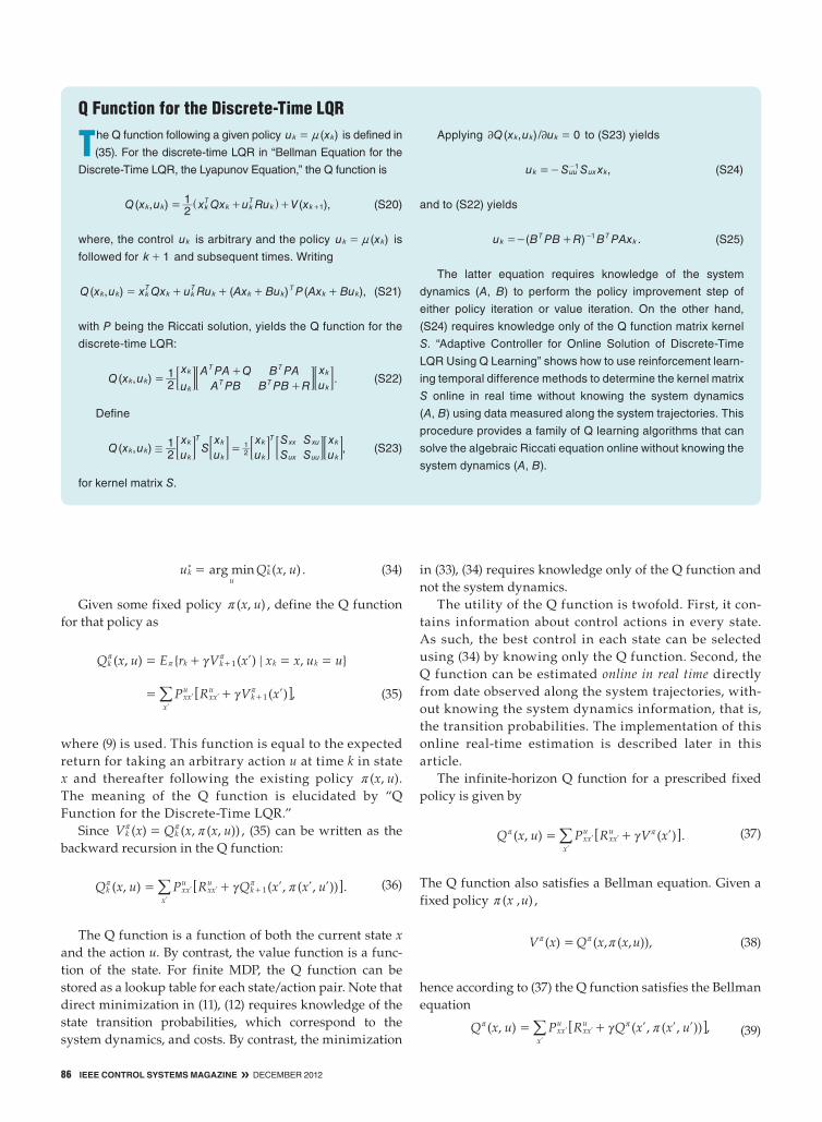
Q Function The conditional expected value in (13),
( , ) ( ) { ( ) , },Q x u P R V x E r V x x x u uk xxu
xxxu
k k k k1 1 k;c c= + = + = =) ) )r+ +l ll
l
l6 @/
( , ) ( ) { ( ) , },Q x u P R V x E r V x x x u uk xxu
xxxu
k k k k1 1 k;c c= + = + = =) ) )r+ +l ll
l
l6 @/ (32)
is known as the optimal Q function [42], [43]. The letter Q comes from “quality function.” The Q function is also called

december 2012 « IEEE CONTROL SYSTEMS MAGAZINE 85
T he bellman equation (17) for the discrete-time LQr is
equivalent to all the formulations (S4), (S6), (S8), (S9) in
“bellman equation for the discrete-Time LQr, the Lyapunov
equation.” Any of these formulations can be used to implement
policy iteration and value iteration.
POLICY ITERATION, hEwER’S ALGORIThM
With step index j, and using superscripts to denote algorithm
steps and subscripts to denote the time k, the iterative policy
evaluation step (25) applied on (S4) in “bellman equation for
the discrete-Time LQr, the Lyapunov equation” yields
( ) ( ) .V x x Qx u Ru V x21j
k kT
k kT
kj
k1 1
1= + ++ ++^ h (S12)
Policy iteration applied on (S6) yields
,x P x x Qx u Ru x P xkT j
k kT
k kT
k kT j
k1
11
1= + +++
++ (S13)
and policy iteration on (S9) yields the Lyapunov equation
( ) ( ) ( ) .A BK P A BK P Q K R K0 j T jj j j j T1 1= - - - + ++ + (S14)
in all cases the policy improvement step is
( )x K xjk
jk
1 1n =+ +
( ),arg min x Qx u Ru x P xkT
k kT
k kT j
k11
1= + + ++
+ (S15)
which can be written explicitly as
( ) .K B P B R B P Aj T T jj1 1 1 1=- ++ + - + (S16)
The policy iteration algorithm format (S14), (S16) relies on
repeated solutions of Lyapunov equations at each step and is
Hewer’s algorithm. This algorithm is proven to converge in [44]
to the solution of the riccati equation (S11) in “The bellman Op-
timality equation for discrete-Time LQr is an Algebraic riccati
equation.” Hewer’s algorithm is an offline algorithm that requires
complete knowledge of the system dynamics (A, B) to find the
optimal value and control. The algorithm requires that the initial
gain K0 be stabilizing.
vALuE ITERATION AND LYAPuNOv RECuRSIONS
Applying value iteration (28) to bellman equation format (S6)
in “bellman equation for the discrete-Time LQr, the Lyapunov
equation” yields
,x P x x Qx u Ru x PkT j
k kT
k kT
k kT
kj1
1 1= + +++ + (S17)
and on format (S9) in “bellman equation for the discrete-Time
LQr, the Lyapunov equation” yields the Lyapunov recursion
( ) ( ) ( ) .P A BK P A BK Q K RKj j T j j j T j1 = - - + ++ (S18)
in both cases the policy improvement step is still given by
(S15), (S16).
The value iteration algorithm format (S16), (S18) is a Ly-
apunov recursion, which is easy to implement and does not,
in contrast to policy iteration, require Lyapunov equation solu-
tions. This algorithm is shown to converge in [45] to the solu-
tion of the riccati equation (S11) in “The bellman Optimality
equation for discrete-Time LQr is an Algebraic riccati equa-
tion.” Lyapunov recursion is an offline algorithm that requires
complete knowledge of the system dynamics (A, B) to find the
optimal value and control. This algorithm does not require that
the initial gain be stabilizing and can be initialized with any
feedback gain.
ONLINE SOLuTION Of ThE RICCATI EquATION wIThOuT
kNOwING ThE PLANT MATRIx A
Hewer’s algorithm and the Lyapunov recursion algorithm are
both offline methods for solving the algebraic riccati equation
(S11) in “The bellman Optimality equation for discrete-Time
LQr is an Algebraic riccati equation.” Full knowledge of the
plant dynamics (A, B) is needed to implement these algo-
rithms. by contrast, both the policy iteration algorithm format
(S13), (S15) and the value iteration algorithm format (S17),
(S15) can be implemented online to determine the optimal val-
ue and control in real time using data measured along the sys-
tem trajectories,and without knowing the system matrix A. This
aim is accomplished through the temporal difference methods
described in the text. That is, reinforcement learning allows the
solution of the algebraic riccati equation online without know-
ing the system matrix A.
Iterative Policy Evaluation
Given a fixed policy K, the iterative policy evaluation procedure
(27) becomes
( ) ( ) .P A BK P A BK Q K RKj T j T1 = - - + ++ (S19)
This recursion converges to the solution to the Lyapunov
equation ( ) ( )P A BK P A BK Q K RKj T T1 = - - + ++ if ( )A BK-
is stable, for any choice of initial value P0 .
Policy Iteration and Value Iteration for the Discrete-Time LQR
the action-value function [5]. The Q function is equal to the expected return for taking an arbitrary action u at time k in state x and thereafter following an optimal policy. The Q function is a function of the current state x and the action u.
In terms of the Q function, the Bellman optimality equation has the particularly simple form
( ) ( , ),minV x Q x uk u k=) ) (33)
86 IEEE CONTROL SYSTEMS MAGAZINE » december 2012
T he Q function following a given policy ( )u xk kn= is defined in
(35). For the discrete-time LQr in “bellman equation for the
discrete-Time LQr, the Lyapunov equation,” the Q function is
( , ) ( ),Q x u x Qx u Ru V x21
k k kT
k kT
k k 1= + + +^ h (S20)
where, the control uk is arbitrary and the policy ( )u xk kn= is
followed for k 1+ and subsequent times. Writing
( , ) ( ) ( ),Q x u x Qx u Ru Ax Bu P Ax Buk k kT
k k k k k kkT T= + + + + (S21)
with P being the riccati solution, yields the Q function for the
discrete-time LQr:
( , ) .Q x ux
uA PA Q
A PBB PA
B PB Rxu2
1k k
k
k
T
T
T
Tk
k=
+
+; ; ;E E E (S22)
define
( , ) ,Q x uxu
Sxu
xu
SS
SS
xu2
1k k
k
k
T k
k
k
k
T xx
ux
xu
uu
k
k21/ =; ; ; ; ;E E E E E (S23)
for kernel matrix S.
Applying ( , ) /Q x u u 0k k k2 2 = to (S23) yields
,u S S xk uu ux k1=- - (S24)
and to (S22) yields
( ) .u B PB R B PAxkT T
k1=- + - (S25)
The latter equation requires knowledge of the system
dynamics (A, B) to perform the policy improvement step of
either policy iteration or value iteration. On the other hand,
(S24) requires knowledge only of the Q function matrix kernel
S. “Adaptive controller for Online Solution of discrete-Time
LQr Using Q Learning” shows how to use reinforcement learn-
ing temporal difference methods to determine the kernel matrix
S online in real time without knowing the system dynamics
(A, B) using data measured along the system trajectories. This
procedure provides a family of Q learning algorithms that can
solve the algebraic riccati equation online without knowing the
system dynamics (A, B).
Q Function for the Discrete-Time LQR
( , )arg minu Q x uku
k=) ) . (34)
Given some fixed policy ( , )x ur , define the Q function for that policy as
( , ) { ( ) , } ( ) ,Q x u E r V x x x u u P R V xk k k k k xxu
xxxu
k1 1;c c= + = = = +rr
r r+ +l ll
l
l6 @/
( , ) { ( ) , } ( ) ,Q x u E r V x x x u u P R V xk k k k k xxu
xxxu
k1 1;c c= + = = = +rr
r r+ +l ll
l
l6 @/ (35)
where (9) is used. This function is equal to the expected return for taking an arbitrary action u at time k in state x and thereafter following the existing policy ( , )x ur . The meaning of the Q function is elucidated by “Q Function for the Discrete-Time LQR.”
Since ( ) ( , ( , ))V x Q x x uk k r=r r , (35) can be written as the backward recursion in the Q function:
( , ) ( , ( , )) .Q x u P R Q x x uk xxu
xxxu
k 1c r= +r r+ l l ll
l
l6 @/ (36)
The Q function is a function of both the current state x and the action u. By contrast, the value function is a func-tion of the state. For finite MDP, the Q function can be stored as a lookup table for each state/action pair. Note that direct minimization in (11), (12) requires knowledge of the state transition probabilities, which correspond to the system dynamics, and costs. By contrast, the minimization
in (33), (34) requires knowledge only of the Q function and not the system dynamics.
The utility of the Q function is twofold. First, it con-tains information about control actions in every state. As such, the best control in each state can be selected using (34) by knowing only the Q function. Second, the Q function can be estimated online in real time directly from date observed along the system trajectories, with-out knowing the system dynamics information, that is, the transition probabilities. The implementation of this online real-time estimation is described later in this article.
The infinite-horizon Q function for a prescribed fixed policy is given by
( , ) ( ) .Q x u P R V xxxu
xxxu
c= +r r ll
l
l6 @/ (37)
The Q function also satisfies a Bellman equation. Given a fixed policy ( , )x ur ,
( ) ( , ( , )),V x Q x x ur=r r (38)
hence according to (37) the Q function satisfies the Bellman equation
( , ) ( , ( , )) ,Q x u P R Q x x uxx
u
xxxu
c r= +r r l l ll
l
l6 @/ (39)

december 2012 « IEEE CONTROL SYSTEMS MAGAZINE 87
the Bellman optimality equation for the Q function is
( , ) ( , ( , )) ,Q x u P R Q x x u'
xxu
xxxu
c r= +) ) )l l ll l6 @/ (40)
( , ) ( , ) .minQ x u P R Q x u'
xxu
xxxu
uc= +) ) l ll l
l8 B/ (41)
Compare (20) and (41), where the minimum operator and the expected value operator are reversed.
Policy iteration and value iteration are especially easy to implement in terms of the Q function (35), as follows.
Policy iteration Using the Q Function
Policy Evaluation (Value Update)
( , ) ( , ( , ))Q x u P R Q x x uj xxu
xxxu
jc r= + l l ll
l
l6 @/ , for all .x X! (42)
Policy Improvement
( , ) ( , )arg minx u Q x uju
j1r =+ , for all .x X! (43)
Value iteration Using the Q Function
Value Update
( , ) ( ', ( ', '))Q x u P R Q x x u''
'j xxu
xxxu
j1 c r= ++ 6 @/ ,
for all .x S Xj! 3 (44)
Policy Improvement
( , ) ( , )arg minx u Q x uju
j1 1r =+ + , for all .x S Xj! 3 (45)
Combining both steps of value iteration yields the form
( , ) ( , )minQ x u P R Q x uj xxu
xxxu
uj1 c= ++ l ll
l
ll
8 B/ ,
for all ,x S Xj! 3 (46)
which may be compared to (31).As shown below, the utility of the Q function is that these
algorithms can be implemented online in real time, without knowing the system dynamics, by measuring data along the system trajectories. These algorithms are an implementation of optimal adaptive control, that is, adaptive control algo-rithms that converge online to optimal control solutions.
Methods for Implementing Policy Iteration and Value IterationMultiple methods are available for performing the value and policy updates for policy iteration and value itera-
tion [5], [6], [17]. The main three methods are exact com-putation, Monte Carlo methods, and temporal difference learning. The last two methods can be implemented without knowledge of the system dynamics. Temporal difference learning, which is covered in the next section, is the means by which optimal adaptive control algo-rithms can be derived for dynamical systems.
Policy iteration requires the solution at each step of Bellman equation (25) for the value update. For a finite MDP with N states, this is a set of linear equations in N unknowns, namely, the values of each state. Value itera-tion requires performing the one-step recursive update (28) at each step for the value update. Both of these itera-tions can be accomplished exactly if the transition proba-bilities { , }PrP x x uxx
u ;= ll and costs Rxxul of the MDP are
known, which corresponds to knowing full system dynamics information. Likewise, the policy improve-ments (26), (29) can be explicitly computed if the dynamics are known. It is shown in “Bellman Equation for the Dis-crete-Time LQR, the Lyapunov Equation” and “The Bell-man Optimality Equation for Discrete-Time LQR Is an Algebraic Riccati Equation” that, for the discrete-time LQR, the exact computation method for computing the optimal control yields the Riccati equation solution approach. In this case policy iteration and value iteration are repetitive solutions of Lyapunov equations or Lyapu-nov recursions. In fact, policy iteration becomes Hewer’s method [44], and the value iteration becomes the Lyapu-nov recursion scheme that is known to converge [45]. These techniques are offline methods that rely on matrix equation solutions and require complete knowledge of the system dynamics.
Monte Carlo learning is based on the definition (16) for the value function and uses repeated measurements of data to approximate the expected value. The expected values are approximated by averaging repeated results along sample paths. An assumption on the ergodicity of the Markov chain with transition probabilities (2) for the given policy being evaluated is implicit. This assumption is suitable for episodic tasks, with experience divided into episodes [5], namely, processes that start in an initial state and run until termination and are then restarted at a new initial state. For finite MDP, Monte Carlo methods converge to the true value function if all states are visited infinitely often. Therefore, to ensure accurate approxima-tions of value functions, the episode sample paths must go through all the states x X! many times. This issue is called the problem of maintaining exploration. Several methods are available to ensure this amount of explora-tion, with one method being the use of exploring starts, in which every state has nonzero probability of being selected as the initial state of an episode.
Monte Carlo techniques are useful for dynamic con-trol because the episode sample paths can be interpreted as system trajectories beginning in a prescribed initial

88 IEEE CONTROL SYSTEMS MAGAZINE » december 2012
state. However, no updates to the value function esti-mate or the control policy are made until after an epi-sode terminates. In fact, Monte Carlo learning methods are closely related to repetitive or iterative learning con-trol [46]. These methods do not learn in real time along a trajectory but learn as trajectories are repeated.
TEMPORAL DIffERENCE LEARNING AND OPTIMAL ADAPTIvE CONTROLIt is now shown that the temporal difference method [5] for solving Bellman equations leads to a family of optimal adaptive controllers, that is, adaptive controllers that learn online the solutions to optimal control problems without knowing the full system dynamics. Temporal difference learning is true online reinforcement learning, wherein control actions are improved in real time based on estimat-ing their value functions by observing data measured along the system trajectories.
Temporal Difference Learning Along State TrajectoriesPolicy iteration requires the solution at each step of N linear equations (25). Value iteration requires performing the recursion (28) at each step. Temporal difference reinforce-ment learning methods are based on the Bellman equation and solve equations such as (25), (28) without using systems dynamics knowledge, but using data observed along a single trajectory of the system. Therefore, temporal differ-ence learning is applicable for feedback control applica-tions. Temporal difference updates the value at each time step as observations of data are made along a trajectory. Periodically, the new value is used to update the policy. Temporal difference methods are related to adaptive con-trol in that they adjust values and actions online in real time along system trajectories.
Temporal difference methods can be considered to be stochastic approximation techniques where by the Bellman equation (17), or its variants (25), (28), is replaced by its eval-uation along a single sample path of the MDP. Then, the Bellman equation becomes a deterministic equation that allows the definition of a temporal difference error.
Equation (9) is used to write the Bellman equation (17) for the infinite-horizon value (16). According to (7)–(9), an alternative form for the Bellman equation is
( ) { } { ( ) } .V x E r x E V x xk k k k k1; ;c= +rr r
r+ (47)
This equation forms the basis for temporal difference learning.
Temporal difference reinforcement learning uses one sample path, namely the current system trajectory, to update the value. Then, (47) is replaced by the deterministic Bellman equation
( ) ( ),V x r V xk k k 1c= +r r+ (48)
which holds for each observed data experience set ( , , )x x rk k k1+ at each time stage k. This data set consists of the current state xk , the observed cost incurred rk , and the next state xk 1+ . The temporal difference error is defined as
( ) ( ),e V x r V xk k k k 1c=- + +r r+ (49)
and the value estimate is updated to make the temporal dif-ference error small.
In the context of temporal difference learning, the interpretation of the Bellman equation is shown in Figure 2, where ( )V xk
r may be considered as a predicted performance or value, rk as the observed one-step reward, and ( )V xk 1c r
+ as a current estimate of future
1) Apply Control Action
2) Update Predicted Value to Satisfy the Bellman Equation
3) Improve Control Action
Observe the 1-Step Reward
Compute Current Estimate of Future Value of Next State xk+1
Compute Predicted Value of Current State xk
k
Vr (xk) = rk + cVr (xk+1)
rk
cVr (xk+1)
Vr (xk)
k+1 Time
FigUre 2 Temporal difference interpretation of the bellman equation that shows how use of the bellman equation captures the action, observation, evaluation, and improvement mechanisms of reinforcement learning.

december 2012 « IEEE CONTROL SYSTEMS MAGAZINE 89
value. The Bellman equation can be interpreted as a con-sistency equation that holds if the current estimate for the predicted value ( )V xk
r is correct. Temporal difference methods update the predicted value estimate ( )V xk
r| to make the temporal difference error small. The idea, based on stochastic approximation, is that if we use the deterministic version of Bellman’s equation repeatedly in policy iteration or value iteration, then on average these algorithms converge toward the solution of the stochastic Bellman equation.
OPTIMAL ADAPTIvE CONTROL fOR DISCRETE-TIME SYSTEMSA family of optimal adaptive control algorithms can now be described for dynamical systems. These algorithms determine the solutions to HJ design equations online in real time without knowing the system drift dynamics. In the LQR case, this means that the algorithms solve the Riccati equation online without knowing the system matrix A. Physical analysis of dynamical systems using Lagrangian mechanics or Hamiltonian mechanics pro-duces system descriptions in terms of nonlinear ordinary differential equations. Discretization yields nonlinear difference equations. Most research in reinforcement learning is conducted for systems that operate in discrete time [5], [14], [21], [39], so discrete-time dynamical systems are covered first, followed by continuous-time systems.
Temporal difference learning is a stochastic approxi-mation technique based on the deterministic Bellman equation (48). Therefore, little is lost by considering deterministic systems here. Consider a class of discrete-time systems described by deterministic nonlinear dynamics in the affine state space difference equation form
( ) ( ) ,x f x g x uk k k k1 = ++ (50)
with state x Rkn! and control input Ruk
m! . This form is used because its analysis is convenient. The following development can be generalized to the sampled-data form
( , )x F x uk k k1 =+ . A deterministic control policy is defined as a function
from state space to control space ( ):h R Rn m"$ . That is, for
every state xk , the policy defines a control action
( )u h xk k= . (51)
That is, a policy is a feedback controller. Define a deterministic cost function that yields the
value function
( ) ( , ) ( ) ,V x r x u Q x u Ruhk
i ki i
i k
i ki i
Ti
i kc c= = +
3 3-
=
-
=
^ h/ / (52)
with 0 11 #c a discount factor, ( )Q x 0k 2 , R 02 , and ( )u h xk k= is a prescribed feedback control policy. That is,
the stage cost is
( , ) ( ) .r x u Q x u Ruk k k kT
k= + (53)
The stage cost is taken as quadratic in uk to simplify the development but can be any positive-definite function of the control. Assume that the system is stabilizable on some set Rn!X , that is, there exists a control policy ( )u h xk k= such that the closed-loop system ( ) ( ) ( )x f x g x h xk k kk1 = ++ is asymptotically stable on X . A control policy ( )u h xk k= is said to be admissible if it is stabilizing and yields a finite cost ( ) .V xh
k
For the deterministic value (52), the optimal value is given by the Bellman optimality equation,
( ) ( , ( )) ( )minV x r x h x V x( )
kh
k k k 1c= +)
$
)+^ h, (54)
which is just the discrete-time HJB equation. The optimal policy is then given as
( ) ( , ( )) ( )arg minh x r x h x V x( )
kh
k k k 1c= +)
$
)+^ h. (55)
In this setup, the deterministic Bellman’s equation (48) is
( ) ( , ) ( )V x r x u V xhk k k
hk 1c= + +
( ) ( ), ( ) ,Q x u Ru V x V 0 0k kT
kh
kh
1c= + + =+ (56)
which is a difference equation equivalent to the value in (52). That is, instead of evaluating the infinite sum (52), the difference equation (56) can be solved, with boundary con-dition V(0) = 0, to obtain the value of using a current policy
( )u h xk k= . The discrete-time Hamiltonian function can be
defined as
( , ( ), ) ( , ( )) ( ) ( ),H x h x V r x h x V x V xk k k k kh
kh
k1cD = + -+ (57)
where ( ) ( )V V x V xk h k h k1T c= -+ is the forward differ-ence operator. The Hamiltonian function captures the energy content along the trajectories of a system as reflected in the desired optimal performance. In fact, the Hamiltonian is the temporal difference error (49). The Bellman equation requires that the Hamiltonian be equal to zero for the value associated with a pre-scribed policy.
For the discrete-time linear quadratic regulator case, the system and Bellman equations are
,x Ax Buk k k1 = ++ (58)
( ) ,V x x Qx u Ru21h
ki k
iT
i iT
ii kc= +
3-
=
^ h/ (59)

90 IEEE CONTROL SYSTEMS MAGAZINE » december 2012
and the Bellman equation can be written in several ways as described in “Bellman Equation for the Discrete-Time LQR, the Lyapunov Equation.”
Policy Iteration and Value Iteration for Discrete-Time Dynamical SystemsTwo forms of reinforcement learning can be based on policy iteration and value iteration. For temporal difference learning, policy iteration is written as follows in terms of the deterministic Bellman equation.
Policy iteration Using Temporal difference Learning
InitializeSelect some admissible control policy ( )h xo k . Starting with j = 0, iterate on j until convergence:
Policy Evaluation
( ) ( , ( )) ( ) .V x r x h x V xj k k j k j k1 1 1c= ++ + + (60)
Policy Improvement
( ) ( , ( )) ( ) ,arg minh x r x h x V x( )
j kh
k k j k1 1 1c= +$
+ + +^ h (61)
or
( ) ( ) ( ),h x R g x V x2j k
Tk j k1
11 14
c=-+
-+ + (62)
where ( ) ( )/V x V x x4 2 2= is the gradient of the value func-tion, interpreted here as a column vector.
Value iteration is similar but with the following policy evaluation procedure.
Value Iteration Using Temporal Difference LearningValue Update Step. Update the value using
( ) ( , ( )) ( ) .V x r x h x V xj k k j k j k1 1c= ++ + (63)
In value iteration, any initial control policy ( )h xk0 can be selected, which is not necessarily admissible or stabilizing.
“Bellman Equation for the Discrete-Time LQR, the Lyapunov Equation” shows that, for the discrete-time LQR, the Bellman equation (56) is a linear Lyapunov equa-tion. “The Bellman Optimality Equation for Discrete-Time LQR Is an Algebraic Riccati Equation” shows that (54) yields the discrete-time algebraic Riccati equation (ARE). For the discrete-time LQR, the policy evaluation step (60) in policy iteration is a Lyapunov equation and policy iteration exactly corresponds to Hewer’s algorithm [44] for solving the discrete-time ARE. Hewer proved that the algorithm converges under stabilizability and detect-ability assumptions. For the discrete-time LQR, value
iteration is a Lyapunov recursion that converges to the solution to the discrete-time ARE under the stated assumptions by [45] (see “Policy Iteration and Value Itera-tion for the Discrete-Time LQR”).
These policy iteration and value iteration algorithms are offline design methods that require knowledge of the dis-crete-time dynamics (A, B). The next section describes online methods for implementing policy iteration and value itera-tion that do not require full dynamics information.
Value Function Approximation Policy iteration and value iteration can be implemented for a finite MDP by storing and updating lookup tables. The key to implementing policy and value iteration online for dynamical systems with infinite state and action spaces is to approximate the value function by a suitable approximator structure in terms of unknown parameters. Then, the unknown parameters are tuned online exactly as in system identification. This idea of value function approximation (VFA) is used by Werbos [14], [19] and called approximate dynamic programming (ADP) or adaptive dynamic programming. The approach is used by Bertsekas and Tsitsiklis [17] and called neurodynamic programming [6], [11].
For nonlinear systems (50), the value function con-tains higher order nonlinearities. We assume the Bell-man equation (56) has a local smooth solution [47]. Then, according to the Weierstrass higher order approximation theorem, there exists a dense basis set { ( )}xi{ such that
( ) ( ) ( ) ( ) ( ) ( ),V x w x w x w x W x xii
i ii
i ii L
iT
L
L
1 1 1/{ { { z f= = + +
3 3
= = = +
/ / /
( ) ( ) ( ) ( ) ( ) ( ),V x w x w x w x W x xii
i ii
i ii L
iT
L
L
1 1 1/{ { { z f= = + +
3 3
= = = +
/ / / (64)
where basis vector ( ) ( ) ( ) ( ) :x x x x R RLn L
1 2 "gz { { {=6 @ and ( )xLf converges uniformly to zero as the number of terms retained L " 3 . The standard usage of the Weier-strass theorem employs a polynomial basis set. In the neural network research, approximation results are shown for other basis sets including sigmoid, hyperbolic tangent, Gaussian radial basis functions, and others. There, stan-dard results show that the neural network approximation error ( )xLf is bounded by a constant on a compact set, where L is the number of hidden-layer neurons, ( )xi{ are the neural network activation functions, and wi are the neural network weights.
In the LQR case, it is known that the value is quadratic in the state, so that ( ) ( / )V x x Px1 2k k
Tk= for some kernel
matrix P. Then the basis set { ( )}xi{ consists of quadratic terms in the state components and the weight vector W consists of the elements of matrix P. Since P is symmetric and has only n(n + 1)/2 independent elements, there are n(n + 1)/2 independent elements in { ( )} .xi{

december 2012 « IEEE CONTROL SYSTEMS MAGAZINE 91
Optimal Adaptive Control Algorithms for Discrete-Time SystemsWith the above background, several adaptive control algo-rithms can be presented based on temporal difference rein-forcement learning that converge online to the optimal control solution.
The parameters in pr or W are unknown. Substitution of the value function approximation ( ) ( )V x W xTz=t into the value update (60) in policy iteration results in the following algorithm.
Optimal Adaptive Control Using a Policy Iteration Algorithm
InitializeSelect some admissible control policy ( )h xk0 . Starting with j = 0, iterate on j until convergence:
Policy Evaluation StepDetermine the least-squares solution Wj 1+ to
( ) ( ) ( , ( )) ( ) ( ) ( ) .W x x r x h x Q x h x Rh xjT
k k k j k k jT
k j k1 1z cz- = = ++ +^ h
( ) ( ) ( , ( )) ( ) ( ) ( ) .W x x r x h x Q x h x Rh xjT
k k j k k jT
k j k1 1z cz- = = ++ +^ h (65)
Policy Improvement Step
Determine an improved policy using
( ) ( ) ( ) .h x R g x x W2j
Tk
Tk j1
11 14
cz=-+
-+ + (66)
This algorithm is easily implemented online by stan-dard system identification techniques [48]. Note that (65) is a scalar equation, whereas the unknown parameter vector W Rj
L1 !+ has L elements. Therefore, data from multiple
time steps are needed for its solution. At time k + 1 we mea-sure the previous state xk , the control ( )u h xk j k= , the next state xk 1+ , and compute the resulting utility ( , ( ))r x h xk j k . These data result in one scalar equation. This procedure is repeated for subsequent times using the same policy ( )hj $ until at least L equations are obtained, at which point the least-squares solution Wj 1+ can be determined. Batch least-squares can be used for this procedure.
Alternatively, note that equations of the form (65) are exactly those solved by recursive least-squares (RLS) tech-niques [48]. Therefore, RLS can be run online until conver-gence. Write (65) as
( ) ( ) ( ) ( , ( )),W k W x x r x h xjT
jT
k k k j k1 1 1/ z czU - =+ + +^ h (67)
with ( ) ( ) ( )k x xk k 1/ z czU - +^ h being a regression vector. At step j of the policy iteration algorithm, the control policy is fixed at ( )u h xj= . Then, at each time k the data set
, , ( , ( ))x x r x h xk k k j k1+^ h is measured. One step of RLS is then performed. This procedure is repeated for subsequent times
until convergence to the parameters corresponding to the value ( ) ( )V x W xj j
T1 1z=+ + . For RLS to converge, the regres-
sion vector ( ) ( ) ( )k x xk k 1/ z czU - +^ h must be persistently exciting.
An alternative to RLS is a gradient descent tuning method such as
( ) ( ) ( ) ( , ( )) ,W W k W k r x h xji
ji
ji T
k j k11
1 1aU U= - -++
+ +^ h (68)
with 02a being a tuning parameter. The step index j is held fixed, and index i is incremented at each increment of the time index k. Note that the quantity inside the large brackets is just the temporal difference error.
Once the value parameters have converged, the control policy is updated according to (66). Then, the procedure is repeated for step j + 1. This entire procedure is repeated until convergence to the optimal control solution.
This method provides an online reinforcement learning algorithm for solving the optimal control problem using policy iteration by measuring data along the system trajec-tories. Likewise, an online reinforcement learning algo-rithm can be given based on value iteration. Substitution of the value function approximation into the value update (63) in value iteration results in the following algorithm.
Optimal Adaptive Control Using a Value Iteration Algorithm
InitializeSelect some control policy ( )h xk0 , not necessarily admis-sible or stabilizing. Starting with j = 0, iterate on j until convergence:
Value Update StepDetermine the least-squares solution Wj 1+ to
( ) ( , ( )) ( ) .W x r x h x W xjT
k k j k jT
k1 1z cz= ++ + (69)
Policy Improvement Step Determine an improved policy using (66).
Equation (69) can be solved in real time using batch least-squares, RLS, or gradient-based methods based on data , , ( , ( ))x x r x h xk k k j k1+^ h measured at each time along the system trajectories. Then the policy is improved using (66). Note that the old weight parameters are on the right-hand side of (69). Thus, the regression vector is now ( )xkz , which must be persistently exciting for convergence of RLS.
Introduction of a Second “Actor” Neural NetworkUsing value function approximation (VFA) allows stan-dard system identification techniques to be used to find the value function parameters that approximately solve the Bellman equation. The approximator structure just described that is used for approximation of the value function is known as the critic neural network, as it

92 IEEE CONTROL SYSTEMS MAGAZINE » december 2012
determines the value of using the current policy. Using VFA, the policy iteration reinforcement learning algo-rithm solves a Bellman equation during the value update portion of each iteration step j by observing only the data set , , ( , ( ))x x r x h xk k k j k1+^ h at each time along the system tra-jectory and solving (65). In the case of value iteration, VFA is used to perform a value update using (69).
The critic network solves the Bellman equation using observed data without knowing the system dynamics. According to “Policy Iteration and Value Iteration for the Discrete-Time LQR,” in the LQR case the critic solves Lyapunov equation (65) or Lyapunov recursions (69) with-out knowing the system matrices (A, B).
Note that in the LQR case the policy update (66) is given by
( ) ,K B P B R B P Aj T j T j1 1 1 1=- ++ + - + (70)
which requires full knowledge of the dynamics (A, B). Note further that the embodiment (66) cannot easily be implemented in the nonlinear case because it is implicit in the control, since xk 1+ depends on h(·) and is the argument of a nonlinear activation function.
These problems are both solved by introducing a second neural network for the control policy, known as the actor neural network [14], [19], [34]. Consider a parametric approxi-mator structure for the control action
( ) ( ),u h x U xk kT
kv= = (71)
with ( ):x R Rn M"v being a vector of M activation functions
and U RM m! # being a matrix of weights or unknown parameters. In the LQR, the optimal state feedback is linear in the states so that the basis set ( )xv can be taken as the state vector.
After convergence of the critic neural network parame-ters to Wj 1+ in policy iteration or value iteration, perform-ing the policy update (66) is required. To achieve this aim, a gradient descent method for tuning the actor weights U such as
( ) ( ) ( ) ( ) ( )U U x R U x g x x W2ji
ji
k ji T
k kT T
k jT
11
1 1 1 14bv v c z= - +++
+ + + +^ h
( ) ( ) ( ) ( ) ( )U U x R U x g x x W2ji
ji
k ji T
k kT T
k jT
11
1 1 1 14bv v c z= - +++
+ + + +^ h (72)
can be used, with 02b being a tuning parameter [34]. The tuning index i can be incremented with the time index k.
The tuning of the actor neural network requires obser-vations at each time k of the data set ( , )x xk k 1+ , that is, the current state and the next state. However, as per the formu-lation (71), the actor neural network yields the control uk at time k in terms of the state xk at time k. The next state xk 1+ is not needed in (71). Thus, after (72) converges, (71) is a legitimate feedback controller. Note that, in the LQR case, the actor neural network (71) embodies the feedback gain
computation (70). Equation (70) contains the state internal dynamics A, but (71) does not. Therefore, the A matrix is not needed to compute the feedback control. The reason is that the actor neural network learns information about A in its weights, since ( , )x xk k 1+ are used in its tuning.
Finally, note that only the input function g(·) or, in the LQR case, the B matrix, is needed in (72) to tune the actor neural network. Introducing a second actor neural network completely avoids the need for knowledge of the state drift dynamics f(·), or the matrix A in the LQR case.
Example 1. Discrete-Time Optimal Adaptive Control of Power System Using Value IterationThis example shows the use of discrete-time value iteration to solve the discrete-time ARE online without knowing the system matrix A. We simulate the online value iteration algo-rithm (69), (72) for load frequency control of an electric power system. Power systems are complicated nonlinear systems. However during normal operation the system load, which produces the nonlinearity, has only small variations. As such, a linear model can be used to represent the system dynamics around an operating point specified by a constant load value. A problem arises from the fact that in an actual plant the parameter values are not precisely known, reflected in an unknown system A matrix, yet an optimal control solution is sought.
The model of the system that is considered here is x Ax Bu= +o , where
, .A
T
RTK
TK
T T
T T
BT
1
0
1
1
0
0
0
1
1
0
0
0
1
0
001
0
P
G
E
P
P
T T
G G
G
=
-
-
- -
- -
=
R
T
SSSSSSS
R
T
SSSSS
V
X
WWWWWWW
V
X
WWWWW
The system state is ( )E t ] ,( )X t 33( )P t( ) [ ( )x t f t g gT3= 3
where ( )f t3 is the incremental frequency deviation in hertz, ( )P tg3 is the incremental change in the generator output (p.u. megawatt), ( )X tg3 is the incremental change in the governor position in p.u. megawatt, and ( )E t3 is the incremental change in integral control. The system param-eters are the governor time constant TG , turbine time con-stant TT , plant model time constant TP , plant model gain KP , speed regulation due to the governor action R, and the integral control gain KE .
The values of the continuous-time system parameters were randomly picked within specified ranges so that
.
..
. .. . ,nA
0 066506 860 6
83 66300
03 66313 736
0
00
13 7360
=
-
-
-
- -
R
T
SSSSS
V
X
WWWWW
. .B 0 0 13 7355 0T = 6 @

december 2012 « IEEE CONTROL SYSTEMS MAGAZINE 93
The discrete-time dynamics were obtained using the zero-order hold method with a sampling period of 0.01 s. The solution to the discrete-time ARE with cost function weights Q I4= , R 1= , and 1c = is
.
.
.
.
.
.
.
.
.
.
.
.
.
.
.
.
.P
0 48050 47720 06040 4771
0 47720 78920 12400 3855
0 06040 12400 05670 0304
0 47710 38550 03042 3513
DARE =
R
T
SSSSS
V
X
WWWWW
In this simulation, only the time constant TG of the gov-ernor, which appears in the B matrix, is considered to be known, while the values for all the other parameters appearing in the system A matrix are not known. That is, the A matrix is needed only to simulate the system and obtain the data and is not needed by the control algorithm.
For the discrete-time LQR, the value is quadratic in the states, ( ) ( / )V x x Px1 2 T= . Therefore, the basis functions for the critic neural network in (64) are selected as the qua-dratic polynomial vector in the state components. Since there are n = 4 states, this vector has ( )/n n 1 2 10+ = com-ponents. The control is linear in the states, u Kx=- , and the basis functions for the actor neural network (71) are taken as the state components.
Value iteration can be implemented online by setting up a batch least-squares problem to solve for the ten critic neural network parameters, which are in the Riccati solu-tion entries Wj 1+ in (69) for each step j. In this simulation, the matrix Pj 1+ corresponding to Wj 1+ is determined after collecting 15 points of data ( , , ( , ))x x r x uk k k k1+ for each least-squares problem. This least-squares problem for the critic weights is solved each 0.15 s. Then the actor neural network parameters, that is, the feedback gain matrix entries, are updated using (72). The simulations were per-formed over a time interval of 60 s.
The system state trajectories are shown in Figure 3, which shows that the states are regulated to zero as desired. The convergence of the Riccati matrix parameters is shown in Figure 4. The final values of the critic neural network parameter estimates are
.
.
.
.
.
.
.
.
.
.
.
.
.
.
.
.
.P
0 48020 47680 06030 4754
0 47680 78870 12390 3843
0 06030 12390 05670 0300
0 47540 38340 03002 3433
critic NN =
R
T
SSSSS
V
X
WWWWW
The optimal adaptive control value iteration algo-rithm converges to the optimal control solution as given by the algebraic Riccati equation solution. This solution is performed in real time without knowing the system A matrix.
Actor-Critic Implementation of Discrete-Time Optimal Adaptive ControlTwo algorithms for optimal adaptive control of dis-crete-time systems based on reinforcement learning have given a policy iteration algorithm implemented by solving (65) using RLS and a policy update by run-ning (72) and a value iteration algorithm implemented by solving (69) using RLS and a policy update by running (72).
The implementation of reinforcement learning using two neural networks, one as a critic and one as an actor, yields the actor/critic reinforcement learning structure shown in Figure 1. In this control system, the critic and the actor are tuned online using the observed data ( , , ( , ( )))x x r x h xk k k j k1+ along the system trajectory. The critic and actor are tuned sequentially in both the policy iteration and the value iteration algorithms. That is, the
0.1
0.08
0.06
0.04
0.02
0
-0.02
-0.04
-0.06
-0.08
-0.10 1 2 3
Time (s)
4 5 6
Sys
tem
Sta
tes
FigUre 3 System states during the first 6 s. This figure shows that, even though the A matrix of the power system is unknown, the adaptive controller based on value iteration keeps the states stable and regulates them to zero.
2.5
2
1.5
1
0.5
0
-0.50 10 20 30
Time (s)
P (1, 1)P (1, 3)P (2, 4)P (4, 4)
40 50 60
P M
atrix
Par
amet
ers
FigUre 4 convergence of selected algebraic riccati equation solution parameters. This plot shows that the adaptive controller based on value iteration converges to the Are solution in real time without knowing the system matrix A.

94 IEEE CONTROL SYSTEMS MAGAZINE » december 2012
This sidebar presents an adaptive control algorithm based
on Q learning that converges online to the solution to the
discrete-time LQr problem. This is accomplished by solving
the algebraic riccati equation in real time without knowing the
system dynamics by using data measured along the system
trajectories.
Q learning is implemented by repeatedly perform-
ing the iterations (79) and (80). in it is seen that the LQr
Q function is quadratic in the states and inputs so that
( , ) ( ) ( / )Q x u Q z z Sz1 2k k k kT
k/= where z x uk kT
kT T
= 6 @ . The ker-
nel matrix S is explicitly given by (S22) in terms of the system
parameters A and B. However, matrix S can be estimated on-
line without knowing A and B by using system identification
techniques. Specifically, write the Q function in parametric
form as
( , ) ( ) ( ),Q x u Q z W zTz= = (S26)
with W being the vector of the elements of S and the basis vector
( )zz consisting of quadratic terms in the elements of z, which
contains state and input components. redundant entries are
removed so that W is composed of the ( ) ( ) /n m n m 1 2+ + +
elements in the upper portion of S, with , .x R u Rkn
km! !
Now, for the LQr, the Q learning bellman equation (79) can
be written as
( ) ( ) ( ) .W z z x Qx u Ru21
jT
k k kT
k kT
k1 1z z- = ++ +^ h (S27)
Note that the Q matrix here is the state weighting matrix in
the performance index; it should not be confused with the Q
function ( ),Q x uk k . This equation must be solved at each step
j of the Q learning process. Note that (S27) is one equation in
( ) /n n 1 2+ unknowns, namely the entries of vector W . This is
exactly the sort of equation encountered in system identifica-
tion, and is solved online using methods from adaptive control
such as recursive least squares (rLS).
Therefore, Q learning is implemented as follows.
INITIALIZE.
Select an initial feedback policy u K xk k0=- at j 0= . The ini-
tial gain matrix need not be stabilizing and can be selected
equal to zero.
STEP j.
Identify the Q Function Using RLS.
At time k, apply the control uk based on the current policy
u K xkj
k=- and measure the data set ( , , , ),x u x uk k k k1 1+ +
where uk 1+ is computed using u K xkj
k1 1=-+ + . com-
pute the quadratic basis sets ( ), ( )z zk k 1z z + . Now per-
form a one-step update in the parameter vector W by
applying rLS to equation (S27). repeat at the next time
k 1+ and continue until rLS converges and the new
parameter vector W j 1+ is found.
Update the Control Policy
Unpack the vector W j 1+ into the kernel matrix
( ) ,Q x uxu
Sxu
xu
SS
SS
xu2
121
,k kk
k
T k
k
k
k
T xx
ux
xu
uu
k
k/ =; ; ; ; ;E E E E E (S28)
Perform the control update using (S24), which is
,u S S xk ux kuu1=- - (S29)
SET j j 1= + . GO TO STEP j.
TERMINATION.
This algorithm is terminated when there are no further updates
to the Q function or the control policy at each step.
This is an adaptive control algorithm implemented using Q func-
tion identification by rLS techniques. No knowledge of the system
dynamics (A, B) is needed for its implementation. The algorithm
effectively solves the algebraic riccati equation online in real-time
using data ( , , )x u x u,k k k k1 1+ + measured in real time at each time
stage k. it is necessary to add probing noise to the control input to
guarantee persistence of excitation to solve (S27) using rLS.
weights of one neural network are held constant while the weights of the other are tuned until convergence. This pro-cedure is repeated until both neural networks have con-verged. Thus, the controller learns the optimal controller online. This procedure amounts to an online adaptive opti-mal control system wherein the value function parameters are tuned online and the convergence is to the optimal value and control. The convergence of value iteration using two neural networks for the discrete-time nonlinear system (50) is proven in [34].
According to reinforcement learning principles, the optimal adaptive control structure requires two loops, a critic and an actor, and operates at multiple timescales. A fast loop implements the control action inner loop, a
slower timescale operates in the critic loop, and a third timescale operates to update the policy.
Q Learning for Optimal Adaptive ControlThe above text described how to implement an optimal adaptive controller using reinforcement learning that only requires knowledge of the system input function ( )g xk . The Q learning reinforcement learning method results in an adaptive control algorithm that converges online to the optimal control solution for completely unknown systems. That is, it solves the Bellman equation (56) and the HJB equation (54) online in real time by using data measured along the system trajectories, without any knowledge of the dynamics ( ), ( )f x g xk k .
Adaptive Controller for Online Solution of Discrete-Time LQR Using Q Learning

december 2012 « IEEE CONTROL SYSTEMS MAGAZINE 95
Q learning, developed by Watkins [42], [43] and Werbos [7], [14], [19], is a simple method for reinforcement learning that works for unknown MDPs, that is for sys-tems with completely unknown dynamics. Q learning is called action-dependent heuristic dynamic programming (ADHDP) by Werbos, since the Q function depends on the control input. Q learning learns the Q function (37) using temporal difference methods by performing an action uk and measuring at each time stage the resulting data expe-rience set ( , , )x x rk k k1+ consisting of the current state, the next state, and the resulting stage cost. Writing the Q function Bellman equation (39) along a sample path gives
( , ) ( , ) ( , ( )),Q x u r x u Q x h xk k k k k k1 1c= +r r+ + (73)
which defines a temporal difference error
( , ) ( , ) ( , ( )) .e Q x u r x u Q x h xk k k k k k k1 1c=- + +r r+ + (74)
The value iteration algorithm for Q function is given by (46). Based on this, the Q function is updated using the algorithm
( , ) ( , ) [ ( , )
( , ) ( , )] .minQ x u Q x u r x u
Q x u Q x uk k k k k k k k k
u k k k k k
1
1 1 1
a
c
= +
+ -
-
- + - (75)
This algorithm is developed for finite MDPs and its conver-gence has been proven by Watkins [42] using stochastic approximation (SA) methods. It is shown the algorithm converges for a finite MDP provided that all state-action pairs are visited infinitely often and
, ,kk
k1
23 31a a=3
=
/ / (76)
which are standard stochastic approximation conditions. On convergence, the temporal difference error is approxi-mately equal to zero. For a finite MDP, Q learning requires storing a lookup table in terms of all the states x and actions u.
The requirement that all state-action pairs are visited infinitely often translates to the problem of maintaining sufficient exploration during learning.
The Q learning algorithm (75) is similar to SA methods for adaptive control or parameter estimation used in the control systems literature. Below is a derivation of methods
for Q learning for dynamical systems that yield adaptive control algorithms that converge to optimal control solutions.
Policy iteration and value iteration algorithms can be given using the Q function in (42)–(46). A Q learning algorithm is easily developed for discrete-time dynam-ical systems using Q function approximation [7], [14], [19], [49]. It is shown in “Q Function for the Dis-crete-Time LQR” that, for the discrete-time LQR, the Q function is a quadratic form in terms of z x uk k
TkT T
/ 6 @ . Assume that, for nonlinear systems, the Q function is parameterized as
( , ) ( ),Q x u W zTz= (77)
for some unknown parameter vector W and basis set vector ( )zz . Substituting the Q function approximation into the
temporal difference error (74) yields
( ) ( , ) ( ),e W z r x u W zkT
k k kT
k 1z c z=- + + + (78)
on which either policy iteration or value iteration algo-rithms can be based. Considering the policy iteration algorithm (42), equation (43) yields the Q function evalua-tion step
( ( ) ( )) ( , ( )),W z z r x h xjT
k k k j k1 1z cz- =+ + (79)
and the policy improvement step
( ) ( , )arg minh x W x uj ku
jT
k1 1z=+ +^ h, for all x X! . (80)
Q learning using value iteration (44) is given by
( ) ( , ( )) ( ),W z r x h x W zjT
k k j k jT
k1 1z c z= ++ + (81)
and (80). These equations do not require knowledge of the dynamics ( ), ( ) .f g$ $
For online implementation, batch least-squares or RLS can be used to solve (79) for the parameter vector Wj 1+ given the regression vector ( ( ) ( ))z zk k 1z cz- + , or (81) using regression vector ( )zkz . The observed data at each time instant are ( , , ( , ))z z r x uk k k k1+ with [ ]z x uk k
TkT T/ . The
vector z x uk kT
kTT
1 1 1/+ + +6 @ is computed using ( )u h xk j k1 1=+ +
A method known as Q learning allows the learning of optimal control solutions
online, in the discrete-time case, for completely unknown systems.

96 IEEE CONTROL SYSTEMS MAGAZINE » december 2012
with ( )hj $ being the current policy. Probing noise must be added to the control input to obtain persistence of excitation. On convergence, the action update (80) is per-formed. This update is easily accomplished without knowing the system dynamics due to the fact that the Q function contains uk as an argument, therefore
( ( , ))/W x u ujT
k12 2z+ can be explicitly computed. The details are presented in.
Due to the simple form of the action update (80), the actor neural network is not needed for Q learning; it can be implemented using only one neural network for Q function approximation.
Approximate Dynamic Programming Using Output FeedbackThe aforementioned methods have relied on full state variable feedback. Little work has been done in applica-tions of reinforcement learning for feedback control using output feedback, which corresponds to partially observable Markov processes. Design of an ADP control-ler that uses only output feedback is given in [50].
INTEGRAL REINfORCEMENT LEARNING fOR OPTIMAL ADAPTIvE CONTROL Of CONTINuOuS-TIME SYSTEMSReinforcement learning is considerably more difficult for continuous-time systems than for discrete-time systems, and fewer results are available. The development of an offline policy iteration method for continuous-time sys-tems is described in [51]. Using a method known as integral reinforcement learning (IRL) [37], [15] allows the application of reinforcement learning to formulate online optimal adaptive control methods for continuous-time systems. These methods find solutions to optimal HJ design equa-tions and Riccati equations online in real time without knowing the system drift dynamics ( )f x , or in the LQR case, without knowing the A matrix.
Consider the continuous-time nonlinear dynamical system
( ) ( ) ,x f x g x u= +o (82)
with state ( )x t Rn! , control input ( )t Ru m! , an equilib-rium point at x 0= , e.g., ( )f 0 0= , and ( ) ( )f g x ux + Lip-schitz on a set Rn3X that contains the origin. Assume that the system is stabilizable on X , that is, there exists a continuous control function ( )u t such that the closed-loop system is asymptotically stable on X .
Define a performance measure or cost function that has the value associated with the feedback control policy
( )u xn= given by
( ( )) ( ( ), ( )) ,V x t r x u dt
x x x=
3
n # (83)
with utility ( , ) ( )r x u Q x u RuT= + , positive-definite ( )Q x , that is, ( )Q x 02 for all x and ( )x Q x0 0&= = , and posi-tive-definite matrix R R RT m m!= # .
For the continuous-time LQR, the above expressions are
,x Ax Bu= +o (84)
( ( )) ( ) .V x t x Qx u Ru d21 T T
t
x= +
3
n # (85)
A policy is called admissible if it is continuous, stabilizes the system, and has a finite associated cost. If the cost is smooth, then an infinitesimal equivalent to (83) can be found by Leibniz’s formula to be
) ( ( ) ( ) ( )), ( ) ,V f x g x x V 0 0n+ =( , ( )) (r x x0 T4n= + n n (86)
where V4 n , taken here as a column vector, denotes the gra-dient vector of the cost function Vn with respect to x.
Equation (86) is the continuous-time Bellman equation. This equation is defined based on the continuous-time Hamiltonian function
) ( ( ) ( ) ( )) .V f x g x xn+) ( , ( )) (V r x x 4n= +( , ( ),H x x T4n n n (87)
The optimal value satisfies the continuous-time (HJB) equation [3]
)V( , ( ),min H x x0 4n= )
n (88)
and the optimal control satisfies
) .V( , ( ),arg min H x x 4n n=) )
n (89)
These expressions show why it is much more challenging to apply reinforcement learning to continuous-time systems. Comparing the continuous-time Hamiltonian (87) to the discrete-time Hamiltonian (57), it is seen that (87) contains the full system dynamics ( ) ( ) ,f x g u u+ whereas (57) does not. What this means is that the continuous-time Bellman equation (86) cannot be used as a basis for reinforcement learning unless the full dynamics are known.
Reinforcement learning methods based on (86) can be developed [52], [29], [40]. These methods have limited use for adaptive control purposes because the system dynamics must be known, state derivatives must be mea-sured, or integration over an infinite horizon is required. In another approach, Euler’s method can be used to discretize the continuous-time Bellman equation (86) (see [52]). Noting that
) ( ( ) ( ) ( ))V f x g x xn+( , ( )) (
( , ( )) ,r x x
r x x V
0 T4n
n
= +
= +
n
no (90)

december 2012 « IEEE CONTROL SYSTEMS MAGAZINE 97
Euler’s forward method can be used to discretize this partial differential equation to obtain
( , )( ) ( ) ( ) ( )
,( , )
r x uT
V x V xT
rT
V x V xx u0 k k
k k k kS k k1 1/= +
-+
-n n n n+ +
( , )( ) ( ) ( ) ( )
,( , )
r x uT
V x V xT
rT
V x V xx u0 k k
k k k kS k k1 1/= +
-+
-n n n n+ + (91)
with sample period T so that t = kT. The discrete sampled utility is ( , ) ( , ) .r x u r x u Tk k k kS =
Now note that the discretized continuous-time Bellman equation (91) has the same form as the discrete-time Bell-man equation (56). Therefore, all the reinforcement learn-ing methods just described for discrete-time systems can be applied.
However, (91) is an approximation only. An alternative exact method for continuous-time reinforcement learn-ing is given in [37], [15]. That method is termed IRL. Note that the cost (83) can be written in the integral reinforce-ment form
( ( )) ( ( ), ( )) ( ( )),V x t r x u d V x t Tt
t T
x x x= + +n n
+
# (92)
for some T > 0. This equation is exactly in the form of the discrete-time Bellman equation (56). According to Bell-man’s principle, the optimal value is given in terms of this construction as [3]
( ( )) ( ( ), ( )) ( ( )) ,minV x t r x u d V x t T( : )u t t T
t
t T
x x x= + +) )
+
+
rf p#
where ( : ) { ( ): } .u t t u t t TT 1#x x+ = +r The optimal con-trol is
( ( )) ( ( ), ( )) ( ( )) .arg minx t r x u d V x t T( : )u t t T t
t T
n x x x= + +) )
+
+
rf p#
It is shown in [37] that the Bellman equation (86) is equiva-lent to the integral reinforcement form (92). That is, the positive-definite solution of both equations is the value (83) of the policy ( )u xn= .
The integral reinforcement form (92) serves as a Bellman equation for continuous-time systems and serves as a fixed point equation. Therefore, the temporal difference error for continuous-time systems can be defined as
( : ) ( ( ), ( )) ( ( )) ( ( )) .e t t T r x u d V x t T V x tt
t T
x x x+ = + + -n n
+
# (93)
This equation does not involve the system dynamics. It is straightforward to use the above equation to for-
mulate policy iteration and value iteration for continu-ous-time systems. The following algorithms are termed as integral reinforcement learning for continuous-time sys-tems [37], [15]. Both algorithms give optimal adaptive controllers for continuous-time systems, that is, adaptive control algorithms that converge to optimal control solutions.
IRL Optimal Adaptive Control Using Policy Iteration
InitializeSelect some admissible control policy ( )x0n . Starting with j = 0, iterate on j until convergence:
Policy Evaluation StepSolve for ( ( ))V x tj 1+ using
( ( )) ( ( ), ( ( ))) ( ( ))V x t r x s x s ds V x t Tj j j
t
t T
1 1n= + ++ +
+
# with ( ) .V 0 0j 1 =+ (94)
Policy Improvement StepDetermine an improved policy using
)],V[ ( , ,arg min H x uju
j1 14n =+ + (95)
which explicitly is
.V( ) ( )x R g x21
jT
j11
14n =-+-
+ (96)
IRL Optimal Adaptive Control Using Value Iteration
InitializeSelect some control policy ( )x0n , which is not necessarily stabilizing. Starting with j = 0, iterate on j until conver-gence.
Policy Evaluation StepSolve for ( ( ))V x tj 1+ using
( ( )) ( ( ), ( ( ))) ( ( )) .V x t r x s x s ds V x t T( )j j j
t
t T
1 n= + ++
+
# (97)
The optimal adaptive controllers presented in this article are a natural
extension of adaptive controllers.

98 IEEE CONTROL SYSTEMS MAGAZINE » december 2012
Policy Improvement StepDetermine an improved policy using (96).
Neither algorithm requires knowledge about the system drift dynamics function ( )f x . That is, the algorithms are applicable to partially unknown systems. Convergence of IRL policy iteration is proved in [37].
Online Implementation of IRL: A Hybrid Optimal Adaptive ControllerBoth of these IRL algorithms can be implemented online by reinforcement learning techniques using value function approximation ( ) ( )V x W xTz= in a critic approximator net-work. Using VFA in the policy iteration algorithm (94) yields
( ( )) ( ( )) ( ( ), ( ( ))) .W x t x t T r x s x s dsjT
j
t
t T
1 z z n- + =+
+
6 @ # (98)
Using VFA in the value iteration algorithm (97) yields
( ( )) ( ( ), ( ( ))) ( ( )) .W x t r x s x s ds W x t TjT
j jT
t
t T
1z n z= + ++
+
# (99)
Then RLS or batch least-squares can be used to update the value function parameters in these equations. On con-vergence of the value parameters, the action is updated using (96).
IRL provides an optimal adaptive controller, that is, an adaptive controller that measures data along the system trajectories and converges to optimal control solutions. Only the system input coupling dynamics g(x) is needed to implement these algorithms. The drift dynamics f(x) is not needed.
The implementation of IRL optimal adaptive control is shown in Figure 5. The time is incremented at each iteration
by the period T. The reinforcement learning time interval T need not be the same at each iteration. The value of T can be changed depending on how long it takes to receive mean-ingful information from the observations; T is not a sample period in the standard meaning.
The measured data at each time increment are ( ( ),x t( ), ( : ))x t T t t Tt+ + where
( : ) ( ( ), ( ))t t T r x u dt
t T
t x x x+ =
+
# (100)
is the integral reinforcement measured on each time interval. The integral reinforcement can be computed in real time by introducing an integrator ( ( ), ( ))r x t u tt =o as shown in Figure 5. That is, the integral reinforcement ( )tt is added as an extra continuous-time state that functions as the memory or controller dynamics. The remainder of the con-troller is a sampled-data controller.
The control policy ( )xn is updated periodically after the critic weights have converged to the solution to (98) or (99). Therefore, the policy is piecewise constant in time. On the other hand, the control varies continuously with the state between each policy update. It is seen that IRL for continu-ous-time systems is in fact a hybrid continuous-time/dis-crete-time adaptive controller that converges to the optimal control solution in real time without knowing the drift dynamics f(x). The optimal adaptive controller has multiple control loops and several timescales. The inner control action loop operates in continuous-time. Data are sampled at intervals of length T. The critic network operates at a slower timescale depending on how long it takes to solve (98) or (99).
Due to the fact that the policy update (96) for continu-ous-time systems does not involve the drift dynamics f(x), no actor neural network is needed in IRL. Only a critic neural network is needed for VFA.
Online Solution of Algebraic Riccati Equation Without Full Plant DynamicsIt can be shown that the integral reinforcement form (92) is equivalent to the Bellman equation (86) [37]. The IRL controller solves the Bellman equation online without knowing the drift dynamics ( )f x . Moreover, IRL con-verges to the optimal control so that it solves the HJB equation (88).
In the continuous-time LQR case (84), (85) the control policies are linear state feedbacks u Kx=- . Then the Bell-man equation (86) is the Lyapunov equation
( ) ( )A BK P P A BK Q K RK 0T T- + - + + = , (101)
and (88) becomes the continuous-time ARE
.A P PA Q PBR B P 0T T1+ + - =- (102)
Update FB GainAfter Critic
Has Converged
Run RLS or Use Batch L.S.to Identify Value of CurrentControl
DynamicControlSystemwithMemory
ZOH T
Critic
T T
Actorn(x)
u xSystemx = f(x) + g(x)u˙
t = r(x(t)), u(t))˙
t
FigUre 5 Hybrid optimal adaptive controller based on integral reinforcement learning (irL), which shows the two-time scale hybrid nature of the irL controller. The integral reinforcement signal is added as an extra state and functions as the memory of the controller. The critic runs on a slow time scale and learns the value of using the current control policy. When the critic converges, the Actor control policy is updated to obtain an improved value.

december 2012 « IEEE CONTROL SYSTEMS MAGAZINE 99
Thus, IRL solves both the Lyapunov equation and the ARE online in real time, using data measured along the system trajectories, without knowing the A matrix.
For the continuous-time LQR, (94) is equivalent to a Lyapunov equation at each step, so that policy iteration is exactly the same as Kleinman’s algorithm [55] for solving the continuous-time Riccati equation. This algorithm is a Newton’s method for finding the optimal value. Continu-ous-time value iteration, on the other hand, is an algorithm that solves the continuous-time ARE based on iterations on certain discrete-time Lyapunov equations that are equiva-lent to (97).
Example 2. Continuous-Time Optimal Adaptive Control Using IRLThis example shows the hybrid control nature of the IRL optimal adaptive controller. It is also shown that IRL finds the solution to the ARE online without solving the ARE and without knowing the system matrix A. Consider the simple dc motor model
. ,x Ax Bu x u10
0 00212
02= + =
-
- -+; ;E E
with cost weight matrices , .Q I R 1= = The solution to the continuous-time ARE is computed to be
..
.
. .P0 05
0 00390 00390 2085=; E
This simulation uses the IRL-based continuous-time value iteration algorithm. This algorithm does not require knowledge of the system matrix A. For the continuous-time LQR, the value is quadratic in the states and the basis functions for the critic neural network are selected as the quadratic polynomial vector in the state components,
( ) .x x x x x12
1 2 22z =6 @ The IRL time interval was selected
as .T 0 04= s. A batch least-squares solution was used to update the three critic weights Wj 1+ , that is, the ARE solu-tion elements, using (99). Measurements of the data set
, , ( : )x t x t T t t Tt+ +^ ^^ h h h are taken over three time inter-vals of .T 0 04= s. Then, provided that there is enough excitation in the system, after each 0.12 s enough data are collected from the system to solve for the value of the matrix P. Then a greedy policy update is performed using (96), that is .u R B Px xKT1 /=- --
The state trajectories in Figure 6 show that suitable regu-lation is achieved. The control input and feedback gains are
shown in Figure 7. The control gains are piecewise con-stant, while the control input is a continuous function of the state between policy updates. The critic neural network parameter estimates are shown in Figure 8. They converge almost exactly to the entries in the Riccati solution matrix P. Thus, the ARE is solved online without knowing the system matrix A.
Adaptive controllers do not generally converge to optimal solutions, and
optimal controllers are designed offline using full dynamics information by
solving matrix design equations.
2
1.5
1
0.5
3.5
3
2.5
4
0
Sys
tem
Sta
tes
Time (s)
0 0.5 1 1.5 2
FigUre 6 System states during the first 2 s, which shows that the continuous-time irL adaptive controller regulates the states to zero without knowing the system matrix A.
Con
trol
Par
amet
ers
Time (s)0 0.5 1 1.5 2
Time (s)
0 0.5 1 1.5 2
-0.2
-0.4
0
Con
trol
Sig
nal
-0.2
-0.1
-0.3
0
FigUre 7 control input and feedback gains, which show the hybrid nature of the irL optimal adaptive controller. The controller gain parameters are discontinuous and piecewise constant, while the con-trol signal itself is continuous between the gain parameter updates.

100 IEEE CONTROL SYSTEMS MAGAZINE » december 2012
Example 3. Continuous-Time Optimal Adaptive Control for Power System Using IRLThis example shows that IRL finds the solution to the ARE online without solving the ARE and without knowing the
system matrix A. Here the continuous-time IRL optimal adaptive control for the electric power system in Example 1 is demonstrated. The same system matrices and perfor-mance index are used as in Example 1. The solution to the continuous-time ARE is computed to be
.
.
.
.
.
.
.
.
.
.
.
.
.
.
.
.
.P
0 47500 47660 06010 4751
0 47660 78310 12370 3829
0 06010 12370 05130 0298
0 47510 38290 02982 3370
ARE =
R
T
SSSSS
V
X
WWWWW
This matrix is close to the discrete-time ARE solution pre-sented in Example 1 since the sample period used there is small.
Both the IRL policy iteration algorithm and the IRL value iteration algorithm are simulated. Neither requires knowl-edge of the system matrix A. The IRL time interval was taken as .T 0 05= s. Note that the IRL interval is not related at all to the sample period used to discretize the system in Example 1. It need not even be taken as a fixed constant for each step. Fifteen data points ( ( ), ( ), ( : ))x t x t T t t Tt+ + were taken to compute each batch least-squares update for the critic parameters Wpj j1 1/+ +r , that is, the elements of the ARE solution P, using (99). The value estimate was updated every .0 75 s. Then, the policy was computed using (96), that is, u R B Px KxT1 /=- -- .
The state trajectories are similar to those presented in Example 1 and so are not plotted here. In the figures show-ing the value function parameter convergence, the star sym-bols represent the true values of the parameters of the optimal cost function calculated by solving the continuous-time ARE. For learning using the IRL policy iteration algo-rithm, the critic parameter estimates for the entries of the P matrix are shown in Figure 9. For learning using the IRL value iteration algorithm, the critic parameter estimates for the P matrix entries are shown in Figure 10. In both cases, the parameters converge to the true solution to the continu-ous-time ARE. Thus, the ARE is solved online without knowing the system A matrix. Note that IRL policy iteration converges far faster than IRL value iteration. Policy iteration is a Newton-Raphson method, so that its convergence rate is quadratic.
Note that far less computation is needed using this IRL algorithm on the continuous-time dynamics than is used in Example 1 for the discrete-time optimal adaptive control algorithm. There, the critic parameter estimates were updated every 0.15 s. Yet, the parameter estimates for the P matrix entries in Figures 4 and 10 almost overlay each other.
Now let’s simulate the effects of changes in the A matrix. At t 30= s, the A matrix was changed to
.
..
. .. . .A
0 066506 860 6
105 66300
05 66313 736
0
00
13 7360
( )t s30 =
-
-
-
- -$
R
T
SSSSS
V
X
WWWWW
Evolution of Cost Function ParametersDuring Learning—Policy Iteration
Time (s)
0
P11P23P24P33P44
0 10 20 30 40 50 60 70
1
2
3
4
5
P11P23P24P33P44
FigUre 9 P matrix parameter estimates for irL policy iteration, which shows that the irL adaptive controller converges online to the optimal riccati equation solution without knowing the system matrix A.
-0.50
P11P23P24P33P44
0 10 20 30 40 50 60 70
0.51
1.52
2.5P11P23P24P33P44
Time (s)
Evolution of Cost Function ParametersDuring Learning—Value Iteration
FigUre 10 P matrix parameter estimates for irL value iteration, which shows that the irL adaptive controller converges online to the optimal riccati equation solution without knowing the system matrix A.
0.05
0.15
0.1
0.2
0
Crit
ic P
aram
eter
s
Time (s)
P(1, 1)P(1, 2)P(2, 2)P(1, 1) – OptimalP(1, 2) – OptimalP(2, 2) – Optimal
0 1 2 3 4 5 6
FigUre 8 P matrix parameter estimates, which shows that the irL adaptive controller converges online to the optimal riccati equa-tion solution without knowing the system matrix A.

december 2012 « IEEE CONTROL SYSTEMS MAGAZINE 101
According to the discussion in Example 1, this corresponds to a change in /K Tp p from eight to ten and of /T1 T from 3.663 to 5.663. The parameters , ,K T TP TP are subject to change on variations in the operating point of the machine, such as what occurs on load changes. For learning using the IRL policy iteration algorithm, the resulting critic parameter estimates for the P matrix entries are shown in Figure 11. For learning using the IRL value iteration algo-rithm, the resulting critic parameter estimates for the P matrix entries are shown in Figure 12. In both cases, the parameters converge after 30 s to the new optimal solution of the ARE corresponding to the new A matrix. This is accomplished without knowing either the old or the new A matrix.
Example 4. Continuous-Time IRL Optimal Adaptive Control for Nonlinear SystemThis example demonstrates the use of IRL to solve the HJB equation for nonlinear continuous-time systems by using data measured along the trajectories in real time. This example was developed using the converse HJB approach [56], which allows construction of nonlinear systems start-ing from the known optimal cost function.
Consider the nonlinear system given by
( ) ( ),
x x x x
x f x g x u
21 1 2 23
2
=- + +
= +
o
o)
with ( ) . ( ) . ( ) , ( )sin sinf x x x x x x g x x0 5 0 5 1 21 2 2 22 2
1 1=- + + + = . With the definitions ( ) ,Q x x x x R2 11
222
24= + + = , then the opti-
mal cost function for this system is ( ) .V x x x x0 5*12
22
24= + +
and the optimal controller is * ( ) ( )sinu x x x x22 123=- + . It
can be verified that the HJB equation and the Bellman equation are both satisfied for these choices.
The cost function is approximated by the smooth function ( ( )) ( ( ))V x t W x tj j
Tz= with L 8= neurons and ( ) [x x x x12
1 2z =
]x x x x x x x x x T22
14
13
2 12
22
1 23
24 . The policy iteration IRL algo-
rithm (98), (96) was used.
To ensure exploration so that the HJB solution is found over a suitable region, data were taken along five trajecto-ries defined by five different initial conditions chosen ran-domly in the region ; ,x i1 1 1 2i# #X = - =" ,. The IRL time period was taken as .T 0 1= s. At each iteration step, a batch least-squares problem was used to solve for the eight neural network weights using 40 data points measured on each of the five trajectories in X . Each data point consisted of ( ), ( ), ( : )x t x t T t t Tt+ +^ hwith ( : )t t Tt + the measured integral reinforcement cost. In this way, at every 4 s, the value was computed and then a policy update was performed.
The result of applying the algorithm is presented in Figure 13, which shows that the parameters of the critic neural network converged to the coefficients of the optimal cost function ( ) .V x x x x0 5*
12
22
24= + + , that is,
. .W 0 5 0 1 0 0 0 0 1 T=6 @ It is observed that after three
iteration steps, that is, after 12 s, the critic neural network parameters have effectively converged. Then, the controller is close to the optimal controller * ( ) ( )sinu x x x x22 12
3=- + . The approximate solution to the HJB equation was determined
Evolution of Cost Function ParametersDuring Learning—Policy Iteration
0 10 20 30 40 50 60 70
Time (s)
3
2
1
0
5
4P11P23P24P33P44
FigUre 11 P matrix parameter estimates for irL policy iteration with a change in the A matrix at 30 s, which shows that the irL adaptive controller converges after 30 s to the new optimal riccati equation solution corresponding to the new A matrix.
Time (s)
Evolution of Cost Function ParametersDuring Learning—Value Iteration
0 2010 30 40 50 7060
1.5
1
0.5
0
-0.5
2.5
2 P11P23P24P33
P44
P11P23P24P33
P44
FigUre 12 P matrix parameter estimates for irL value iteration with a change in the A matrix at 30 s, which shows that the irL adaptive controller converges after 30 s to the new optimal riccati equation solution corresponding to the new A matrix.
1
0.5
0
2.5
2
1.5
3
Crit
ic P
aram
eter
s
Time (s)0 5 10 15 20
w1
w2
w3
w4
w5
w6
w7
w8
w1
w2
w3
w4
w5
w6
w7
w8
FigUre 13 critic neural network parameters, which shows that the irL adaptive controller converges online to the optimal riccati equation solution without knowing the system matrix A.

102 IEEE CONTROL SYSTEMS MAGAZINE » december 2012
online, and optimal control was found without knowing the system drift dynamics ( )f x . Note that analytic solution of the HJB equation in this example would be intractable.
SYNChRONOuS OPTIMAL ADAPTIvE CONTROL fOR CONTINuOuS-TIME SYSTEMSThe aforementioned IRL controller tunes the critic neural network to determine the value while holding the control policy fixed. Then, a policy update is per-formed. Now an adaptive controller is described that has two neural networks, one for value function approximation and one to approximate the control, which could be called the critic neural network and actor neural network. The two neural networks are tuned simultaneously, that is, synchronously in time. This procedure is more nearly in line with accepted practice in adaptive control. Though this synchronous control-ler does require knowledge of the dynamics, it con-verges to the approximate local solutions to the HJB equation and the Bellman equation online, yet does not require explicitly solving either equation. The HJB is usually impossible to solve for nonlinear systems except for special cases.
Based on the continuous-time Hamiltonian (87) and the stationarity condition ( , , )/H x u V u0 2 d 2= n , a policy iteration algorithm for continuous-time systems could be written based on the policy evaluation step
( , ( ), )H x x V0 j j 1dn= + ( , ( )) ( ) ( ( ) ( ) ( )),r x x V f x g x xj j
Tj1dn n= + ++
( )V 0 0j 1 =+ (103)
and the policy improvement step
( , , ) .arg min H x Vj j1 1dn n=n
+ + (104)
Unfortunately, (103) is a nonlinear partial-differential equa-tion and cannot usually be solved analytically.
However, this policy iteration algorithm provides the structure needed to develop another adaptive control algo-rithm that can be implemented online using measured data along the trajectories and converges to the optimal control. Specifically, select a value function approximation (VFA), or critic neural network, structure as
( ) ( )V x W xT1 z= (105)
and a control action approximation structure or actor neural network as
( ) ( ) .u x R g x W21 T T1
2dz=- - (106)
These approximators could be, for instance, two neural networks with unknown parameters or weights ,W W1 2
and ( )xz the basis set or activation functions of the first neural network. The structure of the second action neural network comes from (96). Then tuning the neural network weights as
( )
[ ( ) ],W W Q x u Ru1T
T T1 1 2 1a
v v
vv=-
++ +o (107)
{( ) ( ) ( ) },W F W F W D x W m x W41T T
2 2 2 2 1 1 2 1a v=- - -o r (108)
guarantees stability as well as convergence to the optimal value and control [57].
In these parameter estimation algorithms, , , ,F F1 2 1 2a a are algorithm tuning parameters, ( ) ( ) ( ) ( ) ( ),D x x g x R g x xT T1d dz z= -
( ) ( ) ( ) ( ) ( ),D x x g x R g x xT T1d dz z= - ( ),f gudv z= + /( ),1Tv v v v= +r and ( ) /( ) .m x 1T 2v v v= + A persistency of excitation condi-
tion on ( )tvr is needed to achieve convergence to the opti-mal value.
This synchronous policy iteration controller is an adap-tive control algorithm that requires full knowledge of the system dynamics ( ), ( ),f x g x yet converges to the optimal control solution. That is, the algorithm locally approxi-mately solves the HJB equation, which is usually intracta-ble for nonlinear systems. In the continuous-time LQR case, the algorithm solves the ARE using data measured along the trajectories and knowledge of ( , ) .A B The utility of this algorithm is that it can approximately solve the HJB equation for nonlinear systems using data measured along the system trajectories in real time. The HJB is usually impossible to solve for nonlinear systems except in some special cases.
The VFA tuning algorithm for W1 is based on gradient descent, while the control action tuning algorithm is a form of backpropagation [19] that is, however, also tuned by the VFA weights W1 . This adaptive structure is similar to the actor-critic reinforcement learning structure in Figure 1. However, in contrast to IRL, this algorithm is a continuous-time optimal adaptive controller with two parameter estimators tuned simultaneously, that is, synchronously and continuously in time.
Example 5. Continuous-Time Synchronous Optimal Adaptive ControlThis example demonstrates the use of the synchronous optimal adaptive control algorithm to approximately solve the HJB equation for a nonlinear continuous-time system by using data measured along the trajectories in real time. This example was developed using [56].
Consider the affine in control input nonlinear system ( ) ( ) , ,x f x g x u x R2!= +o where
. ( ( ) )( ) cos
x x
x x xx x x xf x 0 25 2 2
1 2
13
22
12
2 1 13 2
- +
- - - + + +=> H
( )( ) cos x xg x 2 20
1 13+ +
=; E.

december 2012 « IEEE CONTROL SYSTEMS MAGAZINE 103
and select
Q10
01=; E, .R 1=
Then the optimal value function that solves the HJB equation is ( ) . .V x x x0 25 0 5*
14
22= + and the optimal control
policy is ( ) ( ( ) ) .. cosu x x x x2 20 5*1 1
32=- + +
The critic neural network vector activation function are selected as ( ) [ ] .x x x x x1 2
214
242z = The tuning algorithms
(107), (108) were run for the critic neural network and control actor neural network respectively, simultaneously in time. A probing noise was added to the control to guarantee per-sistence of excitation. This noise was decayed exponentially during the simulation. The evolution of the states is shown
in Figure 14. The states are bounded and approach zero as the probing noise decays to zero.
Figure 15 shows the critic parameters, denoted by [ ]W W W W Wc c c c
T1 1 2 3 4= After 80 s, the critic neural net-
work parameters converged to [ . . . . ]( )W t 0 0033 0 4967 0 2405 0 0153fT
1 = [ . . . . ]( )W t 0 0033 0 4967 0 2405 0 0153f
T1 = , which is close to the true weights corre-
sponding to the optimal value ( )V x* that solve the HJB equation. The actor neural network parameters converged to ( ) [ . . . . ] .W t 0 0033 0 4967 0 2405 0 0153f
T2 = The control
policy converged to the optimal control
( ) ( ( ) .cosu x x xx
xx
xW t2
1 02 2
20
02
40
04
T
f21 1
31
2
13
23 2=-
+ +t t; =E G
Figure 16 shows the three-dimensional (3-D) plot of the difference between the approximated value function by using the online synchronous adaptive algorithm, and the optimal value. This error is small relative to the magnitude of the
-0.1
0.5
0.4
0.3
wc1wc2wc3wc4
0.2
0.1
0
0.9
0.8
0.7
0.6
Par
amet
ers
of th
e C
ritic
NN
Time (s)
0 10 20 30 40 50 60 70 80 90 100
FigUre 15 convergence of critic neural network parameters, which shows that the optimal adaptive controller converges to the approximate solution of the nonlinear Hamilton–Jacobi–bellman equation.
-0.04
0.02
0-0.02
0.06
0.04
App
roxi
mat
ion
Err
or o
fth
e V
alue
Fun
ctio
n
2
X2 X1
10-1-2 -2
-10
12
X2
10-1
2 -10
1
FigUre 16 error between optimal and approximated value func-tion. This 3-d plot of the value function error shows that the syn-chronous optimal adaptive controller converges to a value function that is very close to the true solution of the Hamilton–Jacobi–bell-man equation.
-0.2
0
2
X2X1
10-1
-2 -2-1
01
2
-0.1
0.2
0.1
Err
or B
etw
een
Opt
imal
and
App
roxi
mat
ed C
ontr
ol
2
0
X2
10-1 -1
01
2
FigUre 17 error between optimal and approximated control input. This 3-d plot of the feedback control policy error shows that the synchronous optimal adaptive controller converges very close to the true optimal control policy.
-1
0.5
0
x1x2
-0.5
1.5
1
Sys
tem
Sta
tes
Time (s)
0 10 20 30 40 50 60 70 80 90 100
x1x2
FigUre 14 evolution of the states, which shows that the synchro-nous optimal adaptive controller ensures stability and regulates the states to zero.
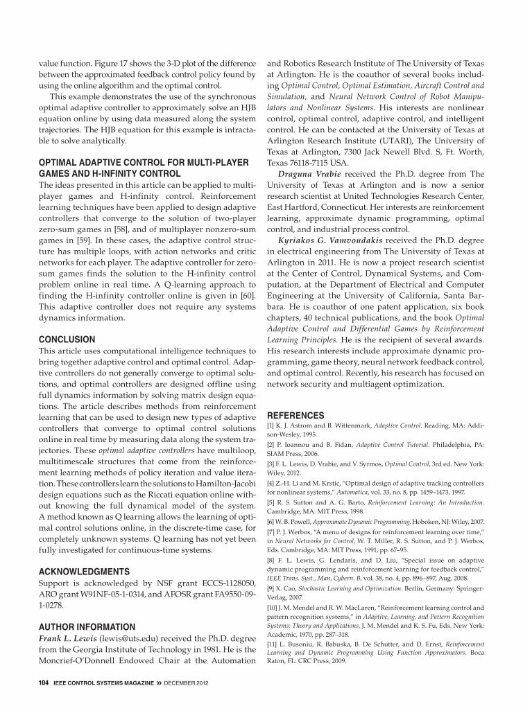
104 IEEE CONTROL SYSTEMS MAGAZINE » december 2012
value function. Figure 17 shows the 3-D plot of the difference between the approximated feedback control policy found by using the online algorithm and the optimal control.
This example demonstrates the use of the synchronous optimal adaptive controller to approximately solve an HJB equation online by using data measured along the system trajectories. The HJB equation for this example is intracta-ble to solve analytically.
OPTIMAL ADAPTIvE CONTROL fOR MuLTI-PLAYER GAMES AND h-INfINITY CONTROLThe ideas presented in this article can be applied to multi-player games and H-infinity control. Reinforcement learning techniques have been applied to design adaptive controllers that converge to the solution of two-player zero-sum games in [58], and of multiplayer nonzero-sum games in [59]. In these cases, the adaptive control struc-ture has multiple loops, with action networks and critic networks for each player. The adaptive controller for zero-sum games finds the solution to the H-infinity control problem online in real time. A Q-learning approach to finding the H-infinity controller online is given in [60]. This adaptive controller does not require any systems dynamics information.
CONCLuSIONThis article uses computational intelligence techniques to bring together adaptive control and optimal control. Adap-tive controllers do not generally converge to optimal solu-tions, and optimal controllers are designed offline using full dynamics information by solving matrix design equa-tions. The article describes methods from reinforcement learning that can be used to design new types of adaptive controllers that converge to optimal control solutions online in real time by measuring data along the system tra-jectories. These optimal adaptive controllers have multiloop, multitimescale structures that come from the reinforce-ment learning methods of policy iteration and value itera-tion. These controllers learn the solutions to Hamilton-Jacobi design equations such as the Riccati equation online with-out knowing the full dynamical model of the system. A method known as Q learning allows the learning of opti-mal control solutions online, in the discrete-time case, for completely unknown systems. Q learning has not yet been fully investigated for continuous-time systems.
ACkNOwLEDGMENTSSupport is acknowledged by NSF grant ECCS-1128050, ARO grant W91NF-05-1-0314, and AFOSR grant FA9550-09-1-0278.
AuThOR INfORMATIONFrank L. Lewis ([email protected]) received the Ph.D. degree from the Georgia Institute of Technology in 1981. He is the Moncrief-O’Donnell Endowed Chair at the Automation
and Robotics Research Institute of The University of Texas at Arlington. He is the coauthor of several books includ-ing Optimal Control, Optimal Estimation, Aircraft Control and Simulation, and Neural Network Control of Robot Manipu-lators and Nonlinear Systems. His interests are nonlinear control, optimal control, adaptive control, and intelligent control. He can be contacted at the University of Texas at Arlington Research Institute (UTARI), The University of Texas at Arlington, 7300 Jack Newell Blvd. S, Ft. Worth, Texas 76118-7115 USA.
Draguna Vrabie received the Ph.D. degree from The University of Texas at Arlington and is now a senior research scientist at United Technologies Research Center, East Hartford, Connecticut. Her interests are reinforcement learning, approximate dynamic programming, optimal control, and industrial process control.
Kyriakos G. Vamvoudakis received the Ph.D. degree in electrical engineering from The University of Texas at Arlington in 2011. He is now a project research scientist at the Center of Control, Dynamical Systems, and Com-putation, at the Department of Electrical and Computer Engineering at the University of California, Santa Bar-bara. He is coauthor of one patent application, six book chapters, 40 technical publications, and the book Optimal Adaptive Control and Differential Games by Reinforcement Learning Principles. He is the recipient of several awards. His research interests include approximate dynamic pro-gramming, game theory, neural network feedback control, and optimal control. Recently, his research has focused on network security and multiagent optimization.
REfERENCES[1] K. J. Astrom and B. Wittenmark, Adaptive Control. Reading, MA: Addi-son-Wesley, 1995.
[2] P. Ioannou and B. Fidan, Adaptive Control Tutorial. Philadelphia, PA: SIAM Press, 2006.
[3] F. L. Lewis, D. Vrabie, and V. Syrmos, Optimal Control, 3rd ed. New York: Wiley, 2012.
[4] Z.-H. Li and M. Krstic, “Optimal design of adaptive tracking controllers for nonlinear systems,” Automatica, vol. 33, no. 8, pp. 1459–1473, 1997.
[5] R. S. Sutton and A. G. Barto, Reinforcement Learning: An Introduction. Cambridge, MA: MIT Press, 1998.
[6] W. B. Powell, Approximate Dynamic Programming. Hoboken, NJ: Wiley, 2007.
[7] P. J. Werbos, “A menu of designs for reinforcement learning over time,” in Neural Networks for Control, W. T. Miller, R. S. Sutton, and P. J. Werbos, Eds. Cambridge, MA: MIT Press, 1991, pp. 67–95.
[8] F. L. Lewis, G. Lendaris, and D. Liu, “Special issue on adaptive dynamic programming and reinforcement learning for feedback control,” IEEE Trans. Syst., Man, Cybern. B, vol. 38, no. 4, pp. 896–897, Aug. 2008.
[9] X. Cao, Stochastic Learning and Optimization. Berlin, Germany: Springer-Verlag, 2007.
[10] J. M. Mendel and R. W. MacLaren, “Reinforcement learning control and pattern recognition systems,” in Adaptive, Learning, and Pattern Recognition Systems: Theory and Applications, J. M. Mendel and K. S. Fu, Eds. New York: Academic, 1970, pp. 287–318.[11] L. Busoniu, R. Babuska, B. De Schutter, and D. Ernst, Reinforcement Learning and Dynamic Programming Using Function Approximators. Boca Raton, FL: CRC Press, 2009.

december 2012 « IEEE CONTROL SYSTEMS MAGAZINE 105
[12] W. Schultz, “Neural coding of basic reward terms of animal learning theory, game theory, microeconomics and behavioral ecology,” Current Opinion Neurobiol., vol. 14, no. 2, pp. 139–147, 2004.
[13] K. Doya, H. Kimura, and M. Kawato, “Neural mechanisms for learning and control,” IEEE Control Syst. Mag., vol. 21, no. 4, pp. 42–54, Aug. 2000.
[14] P. J. Werbos, “Approximate dynamic programming for real-time control and neural modeling,” in Handbook of Intelligent Control, D. A. White and D. A. Sofge, Eds. New York: Van Nostrand Reinhold, 1992.
[15] D. Vrabie and F. L. Lewis, “Neural network approach to continuous-time direct adaptive optimal control for partially-unknown nonlinear sys-tems,” Neural Netw., vol. 22, no. 3, pp. 237–246, Apr. 2009.
[16] A. G. Barto, R. S. Sutton, and C. W. Anderson, “Neuron-like adaptive elements that can solve difficult learning control problems,” IEEE Trans. Syst., Man, Cybern., vol. SMC-13, no. 5, pp. 834–846, Sep./Oct. 1983.
[17] D. P. Bertsekas and J. N. Tsitsiklis, Neuro-Dynamic Programming. Bel-mont, MA: Athena Scientific, 1996.
[18] R. E. Bellman, Dynamic Programming. Princeton, NJ: Princeton Univ. Press, 1957.
[19] P. J. Werbos, “Neural networks for control and system identification,” in Proc. IEEE Conf. Decision Control, Tampa, FL, 1989, pp. 260–265.
[20] D. Prokhorov and D. Wunsch, “Adaptive critic designs,” IEEE Trans. Neural Netw., vol. 8, no. 5, pp. 997–1007, Sep. 1997.
[21] J. Si, A. Barto, W. Powell, and D. Wunsch, Handbook of Learning and Ap-proximate Dynamic Programming. Piscataway, NJ: IEEE Press, 2004.
[22] S. N. Balakrishnan, J. Ding, and F. L. Lewis, “Issues on stability of ADP feedback controllers for dynamical systems,” IEEE Trans. Syst., Man, Cy-bern. B, vol. 38, no. 4, pp. 913–917, Aug. 2008.
[23] F. Y. Wang, H. Zhang, and D. Liu, “Adaptive dynamic program-ming: An introduction,” IEEE Comput, Intell, Mag., vol. 4, no. 2, pp. 39–47, May 2009.
[24] F. L. Lewis and D. Vrabie, “Reinforcement learning and adaptive dy-namic programming for feedback control,” IEEE Circuits Syst. Mag., vol. 9, no. 3, pp. 32–50, 2009.
[25] D. Han and S. N. Balakrishnan, “State-constrained agile missile control with adaptive-critic-based neural networks,” IEEE Trans. Control Syst. Tech-nol., vol. 10, no. 4, pp. 481–489, Jul. 2002.
[26] D. Prokhorov, Computational Intelligence in Automotive Applications. New York: Springer-Verlag, 2008.
[27] S. Ferrari and R. F. Stengel, “An adaptive critic global controller,” in Proc. American Control Conf., May 2002, pp. 2665–2670.
[28] D. Prokhorov, R. A. Santiago, and D. C. Wunsch, II, “Adaptive critic designs: A case study for neurocontrol,” Neural Netw., vol. 8, no. 9, pp. 1367–1372, 1995.
[29] J. J. Murray, C. J. Cox, G. G. Lendaris, and R. Saeks, “Adaptive dynamic pro-gramming,” IEEE Trans. Syst., Man Cybern. C, vol. 32, no. 2, pp. 140–153, 2002.
[30] R. Enns and J. Si, “Helicopter flight control reconfiguration for main rotor actuator failures,” AIAA J. Guidance, Control, Dynamics, vol. 26, no. 4, pp. 572–584, 2003.
[31] C. Lu, J. Si, and X. Xie, “Direct heuristic dynamic programming method for power system stability enhancement,” IEEE Trans. Syst., Man, Cybern. B, vol. 38, no. 4, pp. 1008–1013, 2008.
[32] G. G. Lendaris, L. Schultz, and T. Shannon, “Adaptive critic design for intelligent steering and speed control of a 2-axle vehicle,” in Proc. Int. Conf. Neural Networks, 2000, pp. 73–78.
[33] X. Liu and S. N. Balakrishnan, “Convergence analysis of adaptive critic based optimal control,” in Proc. American Control Conf., June 2000, pp. 1929–1933.
[34] A. Al-Tamimi, F. L. Lewis, and M. Abu-Khalaf, “Discrete-time nonlin-ear HJB solution using approximate dynamic programming: Convergence proof,” IEEE Trans. Syst., Man, Cybern. B, vol. 38, no. 4, pp. 943–949, Aug. 2008.
[35] C. Darwin, On the Origin of Species by Means of Natural Selection. London, U.K.: John Murray, 1859.
[36] D. G. Luenberger, Introduction to Dynamic Systems. New York: Wiley, 1979.
[37] D. Vrabie, O. Pastravanu, M. Abu-Khalaf, and F. L. Lewis, “Adaptive optimal control for continuous-time linear systems based on policy itera-tion,” Automatica, vol. 45, no. 2, pp. 477–484, 2009.
[38] A. Papoulis, Probability Random Variables and Stochastic Processes. New York: McGraw-Hill, 2002.
[39] R. M. Wheeler and K. S. Narendra, “Decentralized learning in finite Mark-ov chains,” IEEE Trans. Autom. Control, vol. 31, no. 6, pp. 519–526, June 1986.
[40] P. Mehta and S. Meyn, “Q-learning and Pontryagin’s minimum princi-ple,” in Proc. IEEE Conf. Decision Control, Dec. 2009, pp. 3598–3605.
[41] H. Zhang, J. Huang, and F. L. Lewis, “Algorithm and stability of ATC receding horizon control,” in Proc. IEEE Symp. Adaptive Dynamic Program-ming Reinforcement, Nashville, TN, Mar. 2009, pp. 28–35.
[42] C. Watkins, “Learning from delayed rewards,” Ph.D. dissertation, Cambridge University, Cambridge, U.K., 1989.
[43] C. J. C. H. Watkins and P. Dayan, “Q-learning,” Mach. Learn., vol. 8, no. 3–4, pp. 279–292, 1992.
[44] G. A. Hewer, “An iterative technique for the computation of the steady state gains for the discrete optimal regulator,” IEEE Trans Autom. Control, vol. 16, no. 4, pp. 382–384, Aug. 1971.
[45] P. Lancaster and L. Rodman, Algebraic Riccati Equations. London, U.K.: Oxford Univ. Press, 1995.
[46] K. L. Moore, Iterative Learning Control for Deterministic Systems. London, U.K.: Springer-Verlag, 1993.
[47] A. J. Van, “L2-gain analysis of nonlinear systems and nonlinear state feed-back H∞ control,” IEEE Trans. Autom. Control, vol. 37, no. 6, pp. 770–784, 1992.
[48] L. Ljung, System Identification: Theory for the User. Englewood Cliffs, NJ: Prentice-Hall, 1999.
[49] S. Bradtke, B. Ydstie, and A. Barto, “Adaptive linear quadratic control using policy iteration,” in Proc. Amer. Control Conf., Baltimore, MD, 1994, pp. 3475–3479.
[50] F. L. Lewis and K. G. Vamvoudakis, “Reinforcement learning for partially observable dynamic processes: Adaptive dynamic programming using measured output data,” IEEE Trans. Syst., Man, Cybern. B, vol. 41, no. 1, pp. 14–25, Feb. 2011.
[51] M. Abu-Khalaf, F. L. Lewis, and J. Huang, “Policy iterations on the Hamilton-Jacobi-Isaacs equation for state feedback control with input satu-ration,” IEEE Trans. Autom. Control, vol. 51, no. 12, pp. 1989–1995, Dec. 2006.
[52] L. C. Baird, “Reinforcement learning in continuous time: Advantage updating,” in Proc. Int. Conf. Neural Networks, Orlando, FL, June1994, pp. 2448–2453.
[53] K. Doya, “Reinforcement learning in continuous time and space,” Neural Comput., vol. 12, no. 1, pp. 219–245, 2000.
[54] T. Hanselmann, L. Noakes, and A. Zaknich, “Continuous-time adap-tive critics,” IEEE Trans. Neural Netw., vol. 18, no. 3, pp. 631–647, May 2007.
[55] D. L. Kleinman, “On an iterative technique for Riccati equation compu-tations,” IEEE Trans. Autom. Control, vol. AC–13, no. 1, pp. 114–115, Feb. 1968.
[56] V. Nevistic and J. Primbs, “Constrained nonlinear optimal control: A converse HJB approach,” Dept. Control Dynamical Systems, California Institute of Technology, Pasadena, CA, Tech. Rep. 96–021, 1996.
[57] K. G. Vamvoudakis and F. L. Lewis, “Online actor-critic algorithm to solve the continuous-time infinite horizon optimal control problem,” Auto-matica, vol. 46, no. 5, pp. 878–888, 2010.
[58] D. Vrabie and F. L. Lewis, “Adaptive dynamic programming for online solution of a zero-sum differential game,” J. Control Theory: Its Appl., vol. 9, no. 3, pp. 353–360, 2011.
[59] K. G. Vamvoudakis and F. Lewis, “Multi-player non-zero sum games: Online adaptive learning solution of coupled Hamilton-Jacobi equations,” Automatica, vol. 47, no. 8, pp. 556–569, 2011.
[60] J. H. Kim and F. L. Lewis, “Model-free H-infinity control design for unknown linear discrete-time systems via Q-learning with LMI,” Auto-matica, vol. 46, no. 8, pp. 1320–1326, Aug. 2010.