Regulatory use of system-wide estimations of PD, LGD and EAD - BIS

Financial Stability Institute

FSI Award 2010 Winning Paper

Regulatory use of system-wide estimations of PD, LGD and EAD Jesus Alan Elizondo Flores Tania Lemus Basualdo Ana Regina Quintana Sordo Comisión Nacional Bancaria y de Valores, Mexico

September 2010

JEL classification: G21, G28

The views expressed in this paper are those of their authors and not necessarily the views of the Financial Stability Institute or the Bank for International Settlements.

Copies of publications are available from:

Financial Stability Institute Bank for International Settlements CH-4002 Basel, Switzerland E-mail: [email protected]

Tel: +41 61 280 9989 Fax: +41 61 280 9100 and +41 61 280 8100

This publication is available on the BIS website (www.bis.org).

© Financial Stability Institute 2010. Bank for International Settlements. All rights reserved. Brief excerpts may be reproduced or translated provided the source is cited.

ISSN 1684-7180

http://www.bis.org/

Foreword

The Financial Stability Institute is pleased to present the winning FSI Award paper for 2010. This award, given every two years at the time of the International Conference of Banking Supervisors, was established to encourage thought and research on issues relevant to banking supervisors globally. In 2010, nine papers were received from central banks and supervisory authorities in eight countries.

A jury of highly qualified individuals read all of the papers and chose the winner. The group was chaired by Mr Jaime Caruana, General Manager of the Bank for International Settlements. It also included Mrs Ruth de Krivoy, former President of the Central Bank of Venezuela; Mr Nick LePan, former Superintendent of Financial Institutions, Canada; Mr Charles Freeland, former Deputy Secretary General of the Basel Committee on Banking Supervision; and Mr Stefan Walter, Secretary General of the Basel Committee on Banking Supervision.

The jury members and the FSI are pleased to announce that the paper authored by Mr Jesus Alan Elizondo Flores, Ms Tania Lemus Basualdo and Ms Ana Regina Quintana Sordo of the Mexican Comisión Nacional Bancaria y de Valores has been chosen as the winner of the 2010 FSI Award. In the paper, the authors set out an example of how to use a prudential tool typically aimed at coping with the solvency of individual banks to deal with the measurement of systemic risk.

Congratulations to our three winners, as well as to the authors of the other papers submitted for consideration. Their interest in analysing and potentially improving supervisory methods provides a true service to the supervisory community.

Josef Tošovský Chairman Financial Stability Institute

September 2010

FSI Award – 2010 Winning Paper i

FSI Award – 2010 Winning Paper iii

Contents

Foreword ..................................................................................... i 1. Introduction ...................................................................... 1 2. System-wide PD, LGD and EAD...................................... 2 3. System-wide information and PD, LGD and EAD

models.............................................................................. 6 4. Empirical results............................................................. 10 5. Model applications ......................................................... 15

5.1 Credit card portfolio reserves............................... 15 5.2 System-wide PD dependency on idiosyncratic

and cyclical factors............................................... 20 5.3 Bank IRB model comparison to system-wide

model estimates................................................... 29 5.4 Risk return analysis of the credit card portfolio.... 32 5.5 Differences in point-in-time (PIT) models and

through-the-cycle (TTC) estimations ................... 38 6. Conclusions.................................................................... 42 Annex 1: Explanatory variables................................................ 44 Annex 2: Reserve requirement rule ......................................... 66 Bibliography.............................................................................. 69

1. Introduction

The objective of prudential regulation has for a long time been the solvency of individual entities and hence a vast range of prudential tools were developed to address this priority. Most recently, due to the period of financial stress and the failure of seemingly solvent institutions, the international supervisory community has expanded the relevance of prudential tools in promoting the stability of the financial system as a whole in addition to individual institutions.

In this sense the Basel Committee has concluded that the issue of systemic risk is probably the most important and most difficult one confronted by the international regulatory community and that progress requires, among other things, a combination of better regulation and the inclusion of a macro perspective into prudential tools.1 With this in mind, the aim of this paper is to extend the use of a prudential tool typically used to cope with the solvency of individual institutions in order to estimate risk parameters that measure systemic risk.

This objective is achieved by estimating system-wide Probability of Default (PD), Loss Given Default (LGD), and Exposure at Default (EAD) parameters for a retail portfolio with information that is representative of the system, both cross-sectionally and for a relevant part of the economic cycle.

This paper intends to generate a prudential tool that (i) encompasses both micro and macro prudential supervision concerns and (ii) sheds light on the adequacy of banks’ individual reserves and their sufficiency to cover systemic expected losses. The tool also seeks to disentangle the nature of exposure of the system to risk, in terms of its dependency on systemic factors, as opposed to idiosyncratic ones.

1 Caruana (2010).

FSI Award – 2010 Winning Paper 1

The paper draws strongly from the recommendations to enhance the resilience of the financial system issued by the Basel Committee in December 2009.2

Particularly, on the loan loss provisioning principles highlighted by the document, in which, among others, it is proposed to: (i) use robust and sound methodologies that reflect expected credit losses in the banks’ existing loan portfolio over the life of the portfolio and (ii) the incorporation of a broader range of available credit information than the one presently included in the incurred loss model to achieve early identification and recognition of losses.

In this paper, the second section defines what is understood by system-wide PD, LGD, and EAD and examines the relevance of its use as a regulatory tool. The third section explains the models used to estimate system-wide parameters and the information used in them. The fourth section provides empirical results. The final section provides practical applications of the regulatory tool for both micro and macroprudential dimensions.

2. System-wide PD, LGD and EAD

In June 2006, the Basel Committee issued the Revised Framework on International Convergence of Capital Measurement and Capital Standards (Basel II),3 which took into account new developments in the measurement and management of banking risks for those institutions that opted to use the “internal ratings-based” (IRB) approach. In this approach, institutions are allowed to use their own internal measures for key drivers of credit risk as primary inputs to the

2 Basel (2009).

3 Basel (2006).

2 FSI Award – 2010 Winning Paper

http://www.bis.org/publ/bcbsca.htm



capital calculation. These measures require the estimation of the following parameters4 that describe the exposure of the portfolio:5

(i) probability of default (PD), which gives the average percentage of obligors that default in a rating grade in the course of one year;

(ii) exposure at default (EAD), which gives an estimate of the outstanding amount (drawn amounts plus likely future draw-downs of yet unused lines) in case the borrower defaults; and

(iii) loss given default (LGD), which gives the percentage of exposure the bank might lose if the borrower defaults.

These risk measures are converted into risk weights and regulatory capital requirements by means of risk weight formulas specified by the Basel Committee.

The parameters mentioned above are aimed at describing the exposure of the bank to its own credit risk. However, the estimation of these parameters can be escalated to consider system-wide information. The interpretation of these parameters gains a broader dimension since explanatory risk factors reflect the potential exposure of the system to a common risk and can be analyzed in two complementary dimensions that offer valuable insight into systemic vulnerabilities (ie cross-sectional and through time).

On the cross-sectional dimension it is acknowledged that a shock hitting one institution can spread to other institutions that are interconnected; thus, such shock can become a systemic threat. This financial shock may be originated from a common exposure across the system.

4 Retail exposures.

5 Basel (2005).


While the use of system-wide estimations of PD, LGD, and EAD may not shed light on the inter-linkages among institutions, it appears to be a useful diagnostic tool for detecting a common exposure to a risk factor across the system.6 The line of investigation that is proposed separates the analysis of system-wide PD into two different branches. On the one hand, we analyze variables associated with individual borrower behaviour; thus such variables are not influenced or under direct control of financial institutions. Examples of these variables are payment behaviour or credit limit use. On the other hand, the variables associated with idiosyncratic factors (individual institution) such as collection and origination practices followed by specific institutions. The hypothesis is that, if system-wide PDs are explained by variables related to the behaviour of individual borrowers and no significant impact is borne by idiosyncratic factors, not only is the system exposed to a common risk exposure but, as long as explanatory factors are dependent on the economic cycle, it is also exposed to cycle dynamics.

In this sense, the procyclical dimension of systemic risk relates to how aggregate risk evolves over time and its dependency on the economic cycle. In order to test if the system is exposed to the time dimension variant of systemic risk, system-wide PDs are correlated to aggregate variables related to the economic cycle and its significance is statistically tested.

Further applications of system-wide PD, LGD, and EAD as a regulatory tool are presented. As mentioned before, the Revised Framework on International Convergence of Capital Measurement and Capital Standards proposes the estimation of capital assuming that expected losses are constituted and

6 However once these parameters are estimated, they can be further used

in subsequent research to explore inter-linkages among institutions using a framework to assess systemic financial stability as defined by Segoviano and Goodhart (2009).




estimated with PD, LGD, and EAD parameters calibrated with the same characteristics (eg 12 months of losses) as those proposed in the Revised Framework. For the case of the country analyzed, it is shown that reserves built by the system at the time of analysis accounted for approximately half of the estimated expected losses under these criteria and were less risk-sensitive. To address this issue a specific reserve requirement based on system-wide estimates of PD, LGD, and EAD was introduced.

It is also shown that the use of system-wide parameters represents a useful benchmarking tool for the validation of IRB models. IRB model estimations of PD calculated by a bank seeking model approval are compared to system-wide estimations of PD. A detailed set of conclusions is drawn on the IRB model proposal and its capacity to consider system-wide explanatory variables of PD.

An additional application is to measure the relevance of using either point-in-time (PIT) model estimates as opposed to through-the-cycle (TTC) models. The analysis of the structure of the model through time indicates the dependency of the aggregate risk of the system to a common set of explanatory variables and provides valuable insight in terms of system vulnerabilities. By using both types of models, it is also shown how system-wide PIT estimations of PD consistently underestimate and overestimate the observed default rates when PIT models are estimated in respectively lower and higher risk segments of the economic cycle.

Finally, a set of conclusions is drawn from individual bank risk pricing practices, as interest rate charging policies can individually be compared to expected loss estimations; thus allowing for risk-return analyses both across banks and within bank portfolios. For the case of the credit card portfolio of the country analyzed, it is concluded that there exists clear price differentiation across banks, generally associated with the risk profile of the population, while it is not the case that pricing practices of all institutions differentiate risk across their own clientele.


3. System-wide information and PD, LGD and EAD models

Models of PD, LGD, and EAD are estimated by banks with information that reflects payment experience within the bank. These parameters tend to describe individual bank experience and often show different explanatory factors when compared to other banks’ models.

In order to convey a system-wide dimension to parameters and identify if there exists common risk factors across banks, three sources of information were collected:

1. Individual credit card statements that describe loan-level data information related to outstanding balance, interest rate, actual payments, minimum required payment, and date of payment. This information is designed to describe the payment behaviour of borrowers, identify recovery in subsequent periods after default and allow the identification of the exposure at the time of default.

2. Credit bureau information that consists of individual credit records, including information such as the number of loans the borrower had with other banks in the analyzed period, its performance and the time elapsed since the borrower first received a loan in the system.

3. Social housing institute information which collects payroll deductions from workers and describes borrowers’ employment history and current income level.

The ten largest institutions, accounting for 97% of total credit cards in the system, were selected to participate in the exercise. A random panel data sample of the system was designed considering two dimensions:

(i) Point-in-time dimension

The information was structured to span a 25-month interval divided into two 12-month intervals and a reference point. The first 12-month interval (historical period) gives information


about the borrower’s behaviour, based on the three sources of information mentioned above, for the twelve months preceding the reference point. The twelve months after the reference point (performance period) are designed to identify individual default rates. This structure allows the association of borrower characteristics and default.

(ii) Time series dimension

To gain insight into the stability of the model through a relevant part of the cycle, 12 windows of 25 months of information were extracted. The 12 reference points selected for each window were April 2006 to March 2007 spanning a three year period of time starting in April 2005 and ending in March 2008.

Random samples were taken from the universe of loans available in the system as registered in the credit bureau for each of the 12 reference points and the size of the sample was determined to allow an estimation error of a PD parameter of 40 basis points with a 99% confidence.7

Default is defined based on the definition of Basel II which states that a loan has defaulted if either one or both of the following events have taken place: (1) the bank considers that the obligor is unlikely to pay its credit obligations to the banking group in full, without recourse by the bank to actions such as realizing security (if held); and (2) the obligor is past due more than 90 days on any material credit obligation to the banking group.

7 The formula used to determine the simple size of the credit card portfolio

is: )1()1(

)1(2

2/2

22/

PPzeN

PPzNn

.


PD model

Categorical data techniques such as logistic regression have increasingly been used in models of prediction of default and this approach is proposed for the estimation of the model of system-wide PD.8

Let be a vector of p independent variables, yi denotes the

value of a dichotomous outcome variable, and i = 1,2,3,…,N. Furthermore, assume that the outcome variable has been coded as 0 or 1, representing the absence or the presence of default, respectively. To fit the logistic regression model

requires the estimation of the vector .

'ix

),...,,( p10'

Let the conditional probability that the outcome is present be

denoted by . The logit of the multiple

logistic regression model is given by the equation

, in which case the logistic

regression model is

)()|1( '' xXYP

ppxxx ...2211xg )( 0'

)'(

)('

'

1)(

xg

xg

e

ex

.

LGD model

LGD is the credit loss incurred if an obligor defaults and is dependent on the characteristics of the loan. Losses are influenced by the presence of collateral and when no collateral exists the cash flows that the borrower pays after default determine the LGD of the loan.

The model proposed to estimate LGD for the credit card portfolio analyzed is to account for the cash flows that occur three months after default and compare them to the maximum outstanding balance of the loan after the moment of default.

8 Hosmer and Lemeshow (1995).


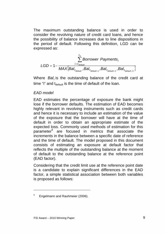
The maximum outstanding balance is used in order to consider the revolving nature of credit card loans, and hence the possibility of balance increases due to line dispositions in the period of default. Following this definition, LGD can be expressed as:

321

3

,,,1

defaultdefaultdefaultdefault

default

tttt

t

tii

BalBalBalBalMAX

PaymentsBorrower

LGD

Where is the outstanding balance of the credit card at

time “i” and tdefault is the time of default of the loan. iBal

EAD model

EAD estimates the percentage of exposure the bank might lose if the borrower defaults. The estimation of EAD becomes highly relevant in revolving instruments such as credit cards and hence it is necessary to include an estimation of the value of the exposure that the borrower will have at the time of default in order to obtain an appropriate estimate of the expected loss. Commonly used methods of estimation for this parameter9 are focused in metrics that associate the increments in the balance between a specific date of reference and the time of default. The model proposed in this document consists of estimating an exposure at default factor that reflects the multiple of the outstanding balance at the moment of default to the outstanding balance at the reference point (EAD factor).

Considering that the credit limit use at the reference point date is a candidate to explain significant differences in the EAD factor, a simple statistical association between both variables is proposed as follows:

9 Engelmann and Rauhmeier (2006).


EAD factor = f (balance at reference point date / credit limit at reference point date)

Where,

EAD factor = balance at default / balance at reference point date.

4. Empirical results

PD model

The independent variables used to build the PD model were constructed from the data set mentioned before and were selected according to their explanatory power. For an exhaustive list of variables analyzed see Annex 1.

The PD model contains the following five variables:

1. X1: number of consecutive periods, up to the reference point, in which the cardholder has not paid its minimum contractual payment obligation;

2. X2: number of periods in which the cardholder has not covered the minimum payment in the last 6 months.

3. X3: payments made by the cardholder as a proportion of the outstanding balance of the credit card at the reference point;

4. X4: total outstanding balance as a proportion of the credit limit at the reference point; and

5. X5: number of months elapsed since the issuance of the credit card by the bank.


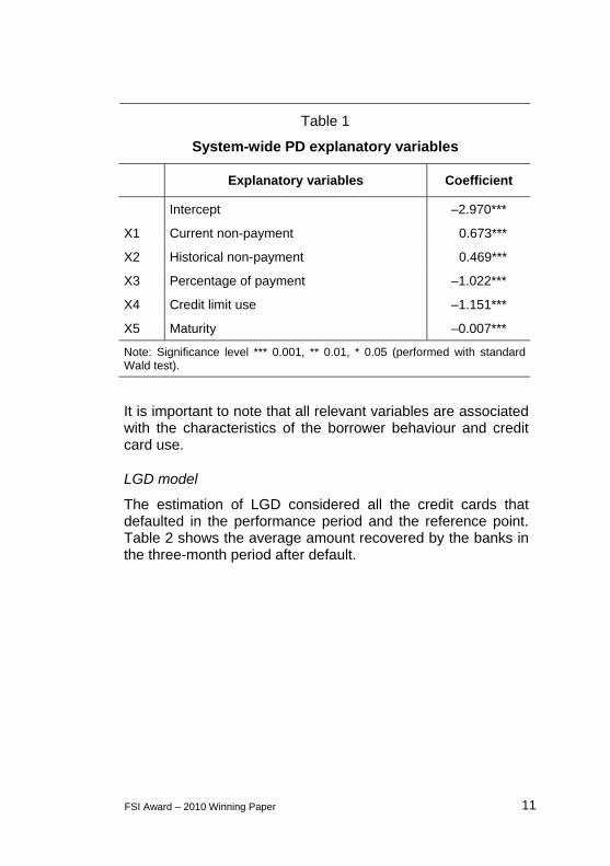
Table 1

System-wide PD explanatory variables

Explanatory variables Coefficient

Intercept –2.970***

X1 Current non-payment 0.673***

X2 Historical non-payment 0.469***

X3 Percentage of payment –1.022***

X4 Credit limit use –1.151***

X5 Maturity –0.007***

Note: Significance level *** 0.001, ** 0.01, * 0.05 (performed with standard Wald test).

It is important to note that all relevant variables are associated with the characteristics of the borrower behaviour and credit card use.

LGD model

The estimation of LGD considered all the credit cards that defaulted in the performance period and the reference point. Table 2 shows the average amount recovered by the banks in the three-month period after default.


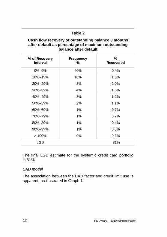
Table 2

Cash flow recovery of outstanding balance 3 months after default as percentage of maximum outstanding

balance after default

% of Recovery Interval

Frequency %

% Recovered

0%–9% 60% 0.4%

10%–19% 10% 1.6%

20%–29% 8% 2.0%

30%–39% 4% 1.5%

40%–49% 3% 1.2%

50%–59% 2% 1.1%

60%–69% 1% 0.7%

70%–79% 1% 0.7%

80%–89% 1% 0.4%

90%–99% 1% 0.5%

> 100% 9% 9.2%

LGD 81%

The final LGD estimate for the systemic credit card portfolio is 81%.

EAD model

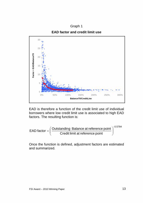
The association between the EAD factor and credit limit use is apparent, as illustrated in Graph 1.


Graph 1

EAD factor and credit limit use

0

5

10

15

20

25

30

0% 50% 100% 150% 200% 250% 300%

BalanceT0/CreditLine

Fa

cto

r =

EA

D/B

ala

nc

eT

0

EAD is therefore a function of the credit limit use of individual borrowers where low credit limit use is associated to high EAD factors. The resulting function is:

5784.0

point reference at limit Credit

point reference at Balance gOutstandinfactor EAD

Once the function is defined, adjustment factors are estimated and summarized.


Table 3

EAD factors as a function of credit limit use

% USE Credit limit

use Mid–point Fitted curve1

0%–10% 5% 566%

10%–20% 15% 300%

20%–30% 25% 223%

30%–40% 35% 184%

40%–50% 45% 159%

50%–60% 55% 141%

60%–70% 65% 128%

70%–80% 75% 118%

80%–90% 85% 110%

90%–100% 95% 103%

>=100% 100% 100% 1 The curve was fitted by OLS by transforming the equation: y = cxb. The significance level of the b parameter (t-test) is .0001.


5. Model applications

5.1 Credit card portfolio reserves

International accounting standard principles have for a long time indicated that credit losses are to be recognized only if there is objective evidence of impairment as a result of a loss event.10

The applicable rule for the country analyzed in this document estimates reserves as a function of the number of past due payments owed by the borrower at the time of analysis.

Table 4

Credit card reserve requirement

Number of periods past due % Reserves

0 0.5%

1 10%

2 45%

3 65%

4 75%

5 80%

6 85%

7 90%

8 95%

9 or more 100%

10 IASB (2009).


While the reserve methodology is easy to implement and reflects more reserves when there is more evidence of loan deterioration, as a prudential requirement, it shows the following limitations:

1. reserves are not calibrated to cover expected losses of 12 months;

2. all relevant available credit information is not considered to differentiate risk among individual borrowers;

3. loss estimations are not based on prospective analysis;

4. the amount of reserves does not consider exposure at default adjustments.

Total loan loss reserves were estimated using the requirement described in Table 4 and contrasted to actual credit card portfolio write-offs for the 12-month period following the estimation.


Table 5

Reserve requirement sufficiency measured in months

12-month write-offs1

Reserves at start of 12-month period1

% Write-offs / Reserves

Months of coverage

Bank 1 2,577 1,045 246.51% 4.9

Bank 2 11,397 5,198 219.26% 5.5

Bank 3 6,650 4,624 143.83% 8.3

Bank 4 629 212 296.69% 4.0

Bank 5 397 212 187.36% 6.4

Bank 6 2,206 1,401 157.44% 7.6

Bank 7 4,001 1,070 373.86% 3.2

Bank 8 534 475 112.39% 10.7

Bank 9 9,392 6,580 142.73% 8.4

Bank 10 543 342 158.58% 7.6

Credit Card System 38,326 21,160 181.12% 6.6

Note: In what follows Bank 1, 2, ..,10 represent the same institution. 1 In millions.

Table 5 shows that reserves were on average sufficient to cover 6.6 months of actual write-offs. The results also illustrate the heterogeneity that the regime generates across banks in terms of the number of months that the allowance covers. This last fact may lead the regulator to consider banks that comply with the regime as equally equipped to cover losses even if there was significant variance among them.


In order to test the exposure of the system, the loan loss distribution of the analyzed portfolio was estimated by using system-wide PD, LGD, and EAD and the IRB capital formulas set in the Revised Framework (Basel II).

Graph 2

Loan loss distribution and capital and reserve requirement

Expected Loss18.42%

Capital Requirement + Reserves (IRB approach)

36.54%

Reserves9.31%

Capital Requirement + Reserves(Standard Approach)

17.31%

F R

E Q

U E

N C

Y

% Assets

8% risk weigthed Assets 18.12 % risk weigthed Assets

Graph 2 makes evident that the regime of reserves along with the Basel I capital standard for the credit card loan portfolio analyzed were insufficient to cover losses measured under the Basel II approach.

System-wide models of PD, LGD, and EAD can be further used to estimate individual banks’ expected losses by feeding corresponding client information on PD and EAD equations. This procedure results in estimates of individual banks’ expected losses and capital estimations illustrated in Table 6.


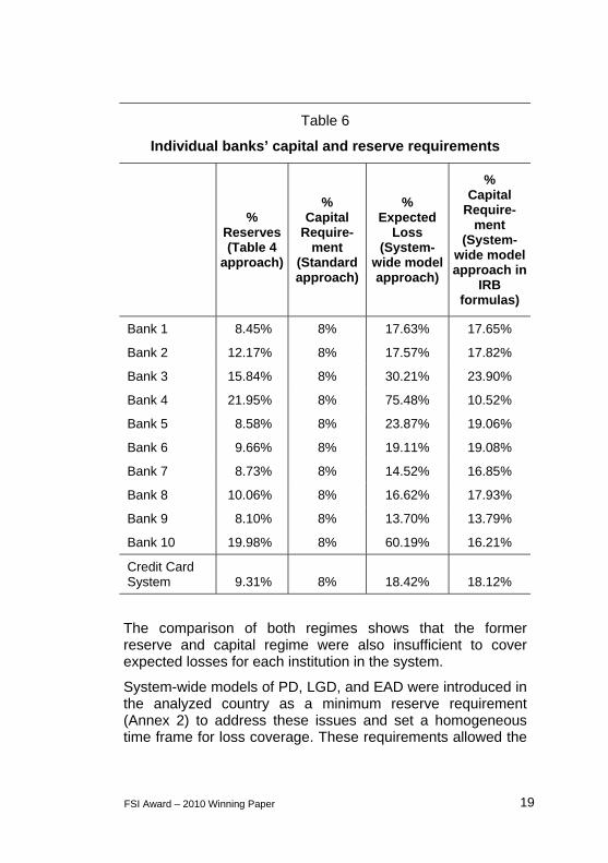
Table 6

Individual banks’ capital and reserve requirements

% Reserves(Table 4

approach)

% Capital

Require-ment

(Standard approach)

% Expected

Loss (System-

wide model approach)

% Capital

Require-ment

(System- wide model approach in

IRB formulas)

Bank 1 8.45% 8% 17.63% 17.65%

Bank 2 12.17% 8% 17.57% 17.82%

Bank 3 15.84% 8% 30.21% 23.90%

Bank 4 21.95% 8% 75.48% 10.52%

Bank 5 8.58% 8% 23.87% 19.06%

Bank 6 9.66% 8% 19.11% 19.08%

Bank 7 8.73% 8% 14.52% 16.85%

Bank 8 10.06% 8% 16.62% 17.93%

Bank 9 8.10% 8% 13.70% 13.79%

Bank 10 19.98% 8% 60.19% 16.21%

Credit Card System 9.31% 8% 18.42% 18.12%

The comparison of both regimes shows that the former reserve and capital regime were also insufficient to cover expected losses for each institution in the system.

System-wide models of PD, LGD, and EAD were introduced in the analyzed country as a minimum reserve requirement (Annex 2) to address these issues and set a homogeneous time frame for loss coverage. These requirements allowed the


regulator to equip the system with a homogeneous regime of reserves fitted to sustain 12 months of expected losses and promoted incentives for banks to develop their own IRB models and to actively manage the risk of their portfolios due to the fact that the regulatory cost of individual loans is more risk sensitive.

5.2 System-wide PD dependency on idiosyncratic and cyclical factors

The credit card portfolio risk exposure of the analyzed country appears to be subject to systemic risk. In order to test the hypothesis of the existence of systemic risk exposure, PD, LGD and EAD models were reinforced with a new set of explanatory variables related to bank idiosyncratic risk and bank exposure to cycle dynamics to detect both potential cross-sectional and procyclical systemic risk exposure.

(i) Cross-sectional dimension

Explanatory variables of the PD model presented in section 4 were shown to be dependent on factors related to individual borrower characteristics and payment behaviour. In order to test the hypothesis of cross-sectional systemic risk due to a common exposure, the proposed next step consisted of testing if banks were a significant explanatory variable in the determination of system-wide PD.

For this purpose, bank portfolios were signalled with a dummy variable that associated each loan to the corresponding bank, and these dummy variables were tested for their significance in the final PD model.


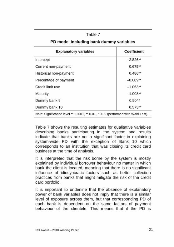
Table 7

PD model including bank dummy variables


Intercept –2.826**

Current non-payment 0.675**

Historical non-payment 0.486**

Percentage of payment –0.009**

Credit limit use –1.063**

Maturity 1.008**

Dummy bank 9 0.504*

Dummy bank 10 0.575**

Note: Significance level *** 0.001, ** 0.01, * 0.05 (performed with Wald Test).

Table 7 shows the resulting estimates for qualitative variables describing banks participating in the system and results indicate that banks are not a significant factor in explaining system-wide PD with the exception of Bank 10 which corresponds to an institution that was closing its credit card business at the time of analysis.

It is interpreted that the risk borne by the system is mostly explained by individual borrower behaviour no matter in which bank the client is located, meaning that there is no significant influence of idiosyncratic factors such as better collection practices from banks that might mitigate the risk of the credit card portfolio.

It is important to underline that the absence of explanatory power of bank variables does not imply that there is a similar level of exposure across them, but that corresponding PD of each bank is dependent on the same factors of payment behaviour of the clientele. This means that if the PD is



different among them it is mostly explained by the fact that the clientele behaviour reflects more risk.

This would imply that the exposure is more dependent on exogenous rather than endogenous factors (or bank-controlled factors) which would in the end result in a higher vulnerability of the system to a common risk exposure.

In order to test further this hypothesis, PD models were built for each participating bank using the corresponding databases. As expected, all the selected variables of the model were significant for all banks and coincident with system-wide estimates of PD.

FS

I Aw

ard – 2010 Winning P

aper 23

Table 8

Individual bank PD model estimates

Intercept Current

Non-Payment

Historical Non-

Payment

Percentage of payment

Credit Limit Use

Maturity ROC

Bank 1 –2.892*** 0.470*** 0.596*** –1.324*** 1.140*** –0.017*** 0.848

Bank 2 –3.595*** 0.677*** 0.522*** –0.646*** 1.583*** –0.008*** 0.834

Bank 3 –3.021*** 0.509*** 0.428*** –0.625*** 1.104*** –0.005*** 0.796

Bank 4 –0.908*** 0.711*** 0.405*** –0.743*** 0.725*** –0.043*** 0.796

Bank 5 –2.665*** 0.553*** 0.499*** 1.339*** 1.676*** –0.076*** 0.841

Bank 6 –2.381*** 0.630*** 0.536*** –1.084*** 0.761*** –0.11*** 0.844

Bank 7 –3.674*** 0.643*** 0.563*** –0.829*** 1.864*** –0.004*** 0.877

Bank 8 –3.146*** 0.515*** 0.529*** –1.400*** 1.850*** –0.007*** 0.844

Bank 9 –3.394*** 0.570*** 0.629*** –0.565*** 0.856*** –0.006*** 0.855

Bank 10 –1.448*** 0.597*** 0.351*** –0.273*** 0.764*** –0.048*** 0.767

Note: Significance level *** 0.001, ** 0.01, * 0.05.

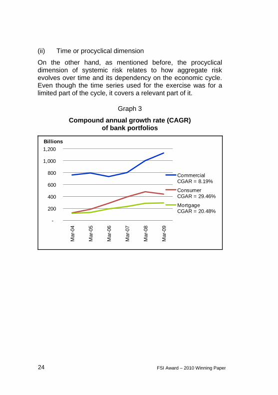
(ii) Time or procyclical dimension

On the other hand, as mentioned before, the procyclical dimension of systemic risk relates to how aggregate risk evolves over time and its dependency on the economic cycle. Even though the time series used for the exercise was for a limited part of the cycle, it covers a relevant part of it.

Graph 3

Compound annual growth rate (CAGR) of bank portfolios

-

200

400

600

800

1,000

1,200

Mar

-04

Mar

-05

Mar

-06

Mar

-07

Mar

-08

Mar

-09

Billions

CommercialCGAR = 8.19%

ConsumerCGAR = 29.46%

MortgageCGAR = 20.48%


Graph 4

Consumer credit past due loan ratio

3.2%

8.8%

2.6%

4.5%

1.3%

4.9%

0%

1%

2%

3%

4%

5%

6%

7%

8%

9%

10%

11%

12%

13%

Dec-04 Dec-05 Dec-06 Dec-07 Dec-08 Dec-09

Delinquency Index(Past Due Loans / Total Balance ) of consumer loans

portfolio

Credit Cards

Consumer Credit

Other**

Graphs 3 and 4 illustrate the strong period of growth of consumer credit portfolios during the period under review which was matched to an increasing deterioration rate of the credit card portfolio.

The effect of higher levels of leverage across households resulted in deteriorating credit quality, not only for newly originated loans, which showed less experience in handling credit, but also for customers that were already in the portfolio and increased their indebtedness by contracting new credit cards offered by competitors.


Graph 5

Household indebtedness

Credits per Person by Credit Type

3

3.2

3.4

3.6

3.8

4

4.2

4.4

D2005

E

F M A M2006

J

J A S O N D E F M A M2007

J

J A S O N

1.00

1.05

1.10

1.15

1.20

1.25

1.30

1.35

1.40

Bank credt cards (left axis) Mortgage (right axis) Car (right axis)

Monthly Average Debt-Capacity per Debtor

(Sample)

0

100,000

200,000

300,000

400,000

500,000

600,000

700,000

800,000

900,000

1 2 3 4 5 6 7 8Number of Credit Cards

MXN pesos

Dec. 2005 Nov. 2007


In order to test the time dimension exposure to systemic risk and considering the relative time series limitations of data, two time series of data were built and added to the panel data sample that reflected different aspects of the economic cycle. On the one hand, the increase of competition that was approximated by the number of institutions operating in the system. On the other hand the relative experience of the system in managing debt, measured by the average age of borrowers extracted from the credit bureau database.

Graph 6

Number of institutions offering credit card loans

Number of Institutions

13

14

15

16

17

18

2006

04

2006

05

2006

06

2006

07

2006

08

2006

09

2006

10

2006

11

2006

12

2007

01

2007

02

2007

03

10%

12%

14%

16%

18%

20%

Def

ault

rat

e

Number of Institutions Default rate


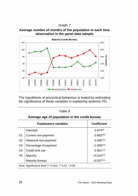
Graph 7

Average number of months of the population in each time observation in the panel data sample

Maturity Credit Bureau

80

85

90

95

100

105

2006

04

2006

05

2006

06

2006

07

2006

08

2006

09

2006

10

2006

11

2006

12

2007

01

2007

02

2007

03

10%

12%

14%

16%

18%

20%

Def

ault

rat

e

Maturity Bureau Default rate

The hypothesis of procyclical behaviour is tested by estimating the significance of these variables in explaining systemic PD.

Table 9

Average age of population in the credit bureau


Intercept 0.874**




X4 Credit limit use 0.951***


Maturity bureau –0.037***



Table 10

Number of institutions offering credit card loans


Intercept –3.706***




X4 Credit limit use 0.936***


Number of institutions 0.082***


Tables 9 and 10 provide evidence of significant correlation of these variables with systemic PD showing dependence on variables that reflect relevant aspects of the cycle.

Even though evidence is not conclusive as only one part of the cycle is considered for analysis, this line of investigation offers room for further work as the identification of significant variables may shed future light on early warning mechanisms of risk build-up in the system.

5.3 Bank IRB model comparison to system-wide model estimates

The analyzed country has implemented the Basel II capital framework, allowing banks to use IRB models to estimate capital requirements. Banks that opt to follow this approach have to document their model and are subject to approval for use.

An internal model developed by a bank that participates in credit card business has been subject to the approval process


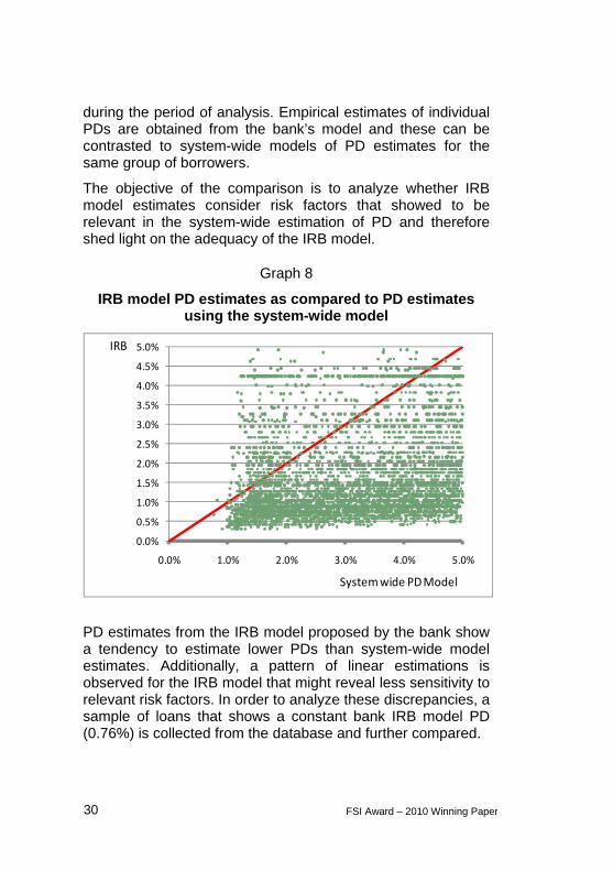
during the period of analysis. Empirical estimates of individual PDs are obtained from the bank’s model and these can be contrasted to system-wide models of PD estimates for the same group of borrowers.

The objective of the comparison is to analyze whether IRB model estimates consider risk factors that showed to be relevant in the system-wide estimation of PD and therefore shed light on the adequacy of the IRB model.

Graph 8

IRB model PD estimates as compared to PD estimates using the system-wide model

0.0%

0.5%

1.0%

1.5%

2.0%

2.5%

3.0%

3.5%

4.0%

4.5%

5.0%

0.0% 1.0% 2.0% 3.0% 4.0% 5.0%

IRB

System wide PD Model

PD estimates from the IRB model proposed by the bank show a tendency to estimate lower PDs than system-wide model estimates. Additionally, a pattern of linear estimations is observed for the IRB model that might reveal less sensitivity to relevant risk factors. In order to analyze these discrepancies, a sample of loans that shows a constant bank IRB model PD (0.76%) is collected from the database and further compared.


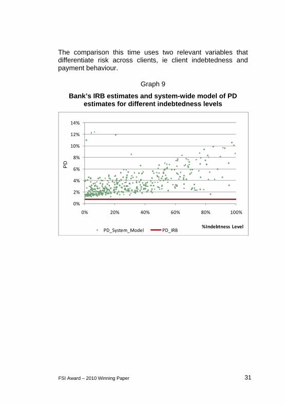
The comparison this time uses two relevant variables that differentiate risk across clients, ie client indebtedness and payment behaviour.

Graph 9

Bank’s IRB estimates and system-wide model of PD estimates for different indebtedness levels

0%

2%

4%

6%

8%

10%

12%

14%

0% 20% 40% 60% 80% 100%

PD

%Indebtness LevelPD_System_Model PD_IRB


Graph 10

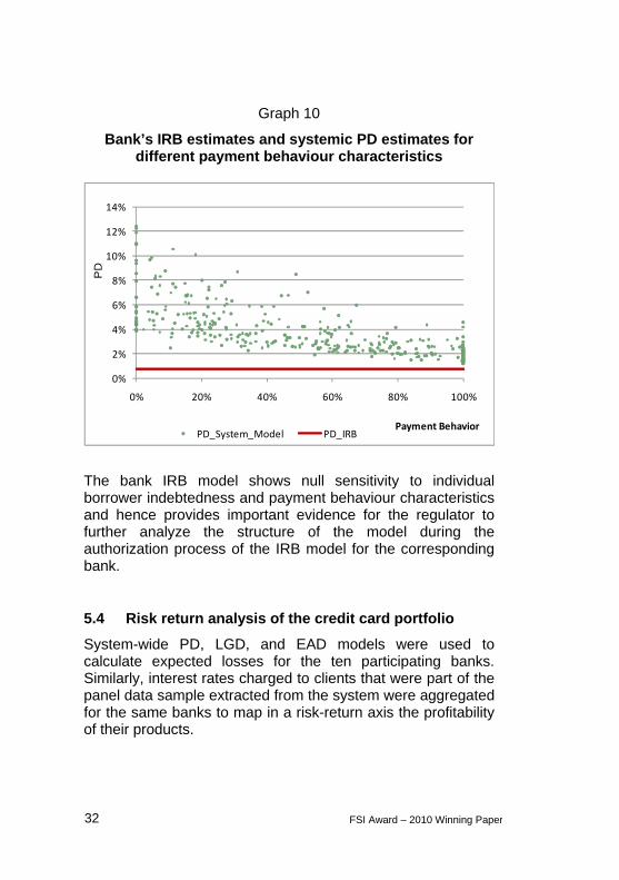
Bank’s IRB estimates and systemic PD estimates for different payment behaviour characteristics

0%

2%

4%

6%

8%

10%

12%

14%

0% 20% 40% 60% 80% 100%

PD

Payment BehaviorPD_System_Model PD_IRB

The bank IRB model shows null sensitivity to individual borrower indebtedness and payment behaviour characteristics and hence provides important evidence for the regulator to further analyze the structure of the model during the authorization process of the IRB model for the corresponding bank.

5.4 Risk return analysis of the credit card portfolio

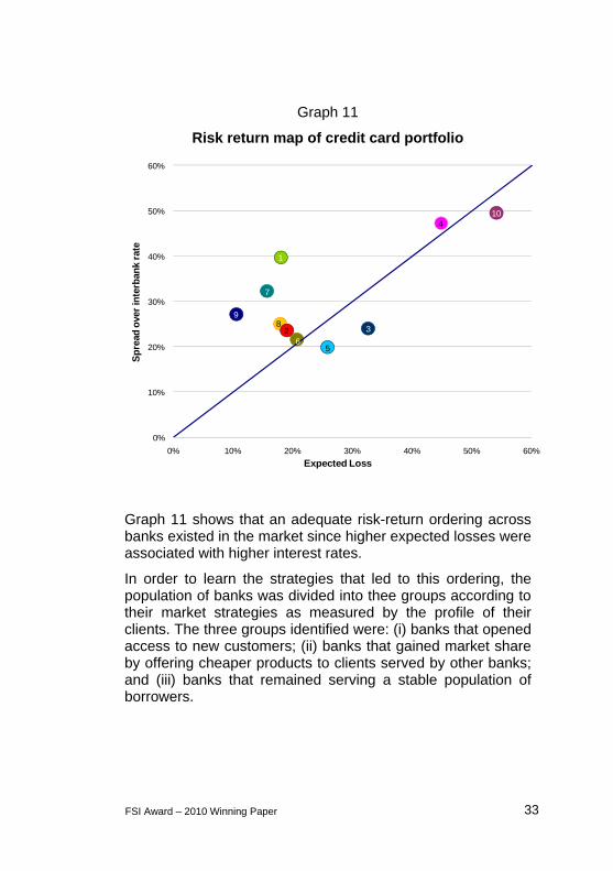
System-wide PD, LGD, and EAD models were used to calculate expected losses for the ten participating banks. Similarly, interest rates charged to clients that were part of the panel data sample extracted from the system were aggregated for the same banks to map in a risk-return axis the profitability of their products.


Graph 11

Risk return map of credit card portfolio

0%

10%

20%

30%

40%

50%

60%

0% 10% 20% 30% 40% 50% 60%

Sp

read

ove

r in

terb

ank

rate

Expected Loss

Precio excesivo

4

5

32

7

10

9

6

8

1

Graph 11 shows that an adequate risk-return ordering across banks existed in the market since higher expected losses were associated with higher interest rates.

In order to learn the strategies that led to this ordering, the population of banks was divided into thee groups according to their market strategies as measured by the profile of their clients. The three groups identified were: (i) banks that opened access to new customers; (ii) banks that gained market share by offering cheaper products to clients served by other banks; and (iii) banks that remained serving a stable population of borrowers.


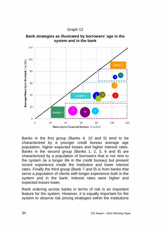
Graph 12

Bank strategies as illustrated by borrowers’ age in the system and in the bank

Banks in the first group (Banks 4, 10 and 5) tend to be characterized by a younger credit bureau average age population, higher expected losses and higher interest rates. Banks in the second group (Banks 1, 2, 3, 6 and 8) are characterized by a population of borrowers that is not new to the system (ie a longer life in the credit bureau) but present recent experience inside the institution and lower interest rates. Finally the third group (Bank 7 and 9) is from banks that serve a population of clients with longer experience both in the system and in the bank. Interest rates were higher and expected losses lower.

Rank ordering across banks in terms of risk is an important feature for the system. However, it is equally important for the system to observe risk pricing strategies within the institutions


that consider individual borrower’s risk and hence transmit adequate interest rates to clients.

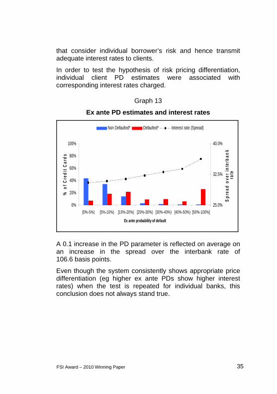
In order to test the hypothesis of risk pricing differentiation, individual client PD estimates were associated with corresponding interest rates charged.

Graph 13

Ex ante PD estimates and interest rates

0%

20%

40%

60%

80%

100%

[0%-5%) [5%-10%) [10%-20%) [20%-30%) [30%-40%) [40%-50%) [50%-100%]

Ex ante probability of default

% o

f C

red

it C

ard

s

25.0%

32.5%

40.0%

Sp

read

ove

r in

terb

ank

rate

Non Defaulted* Defaulted* Interest rate (Spread)

A 0.1 increase in the PD parameter is reflected on average on an increase in the spread over the interbank rate of 106.6 basis points.

Even though the system consistently shows appropriate price differentiation (eg higher ex ante PDs show higher interest rates) when the test is repeated for individual banks, this conclusion does not always stand true.


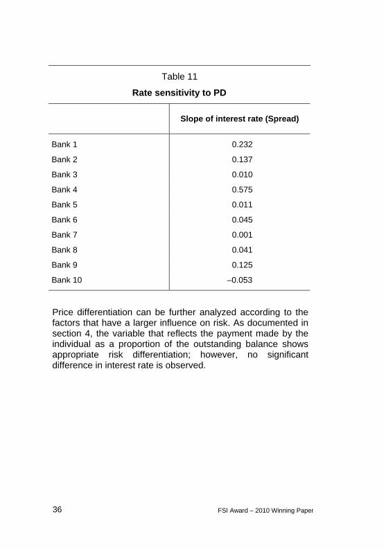
Table 11

Rate sensitivity to PD

Slope of interest rate (Spread)

Bank 1 0.232

Bank 2 0.137

Bank 3 0.010

Bank 4 0.575

Bank 5 0.011

Bank 6 0.045

Bank 7 0.001

Bank 8 0.041

Bank 9 0.125

Bank 10 –0.053

Price differentiation can be further analyzed according to the factors that have a larger influence on risk. As documented in section 4, the variable that reflects the payment made by the individual as a proportion of the outstanding balance shows appropriate risk differentiation; however, no significant difference in interest rate is observed.


Graph 14

Risk price differentiation across the system according to client’s percentage of payment

20%

36%

52%

0%

20%

40%

60%

80%

100%

[0%-10%) [10%-20%) [20%-40%) [40%-60%) [60%-80%) [80%-100%] >100% Sp

read

over

inte

rban

k r

ate

% o

f C

red

it C

ard

s

Percentage of Payment

Non defaulted* Defaulted* Interest rate (Spread)

Similarly the degree of indebtedness of the borrower was shown to be a relevant risk factor; although no significant difference in credit card interest rate is observed.

Graph 15

Client indebtedness risk price differentiation across the system

20.00%

36.00%

52.00%

0%

20%

40%

60%

80%

100%

[0%-10%) [10%-20%) [20%-40%) [40%-60%) [60%-80%) [80%-100%] >100%

Sp

read

over

inte

rban

k r

ate

% o

f C

red

it C

ard

s

Credit Limit Use

Non Defaulted* Defaulted* Interest rate (Spread)


The introduction of reserve requirements that reflect direct exposure to system-wide variables is expected to generate regulatory incentives for banks to start risk pricing strategies among institutions that will promote more competition in the system.

The analysis presented resulted in benefits to the regulator since it generated relevant discussions with banks on pricing strategies, risk management capacities and broader topics related to competitiveness in the credit card business.

5.5 Differences in point-in-time (PIT) models and through-the-cycle (TTC) estimations

Models for PD estimation can be calculated with information from one period (one 25-month window of time) as “point-in-time” (PIT) estimates or, in line with the Revised Framework, “through-the-cycle” (TTC) by considering information from a longer period. TTC systems are expected to estimate more stable PDs over the cycle.

In order to test the differences in PIT and TTC models for the portfolio analyzed, two additional models were estimated by using separate data from two different reference dates (April 2006 and February 2007).


Table 12

PIT and TTC model estimates

Model estimation using only information from April 2006

Explanatory variables Coefficient Wald Confidence

Level (95%)

Intercept –3.386** –3.744 –3.028

Current non-payment 0.682** 0.494 0.870

Historical non-payment 0.541** 0.431 0.650

Percentage of payment –0.245* –0.720 0.229

Credit limit use 1.277** 0.932 1.623

Maturity –0.009** –0.012 –0.006

Model estimation using only information from February 2007


Level (95%)

Intercept –2.395** –2.620 –2.169



Percentage of payment –0.724** –1.033 –0.415

Credit limit use 1.094** 0.861 1.327

Maturity –0.014** –0.017 –0.011



Table 12 (cont)

PIT and TTC model estimates

Model estimation using all windows (proposed model)


Level (95%)

Intercept –2.970** –3.054 –2.887



Percentage of payment –1.022** –1.131 –0.912

Credit limit use –1.151** 1.074 1.228

Maturity –0.007** –0.008 –0.007


Evidence from the estimations of PIT and TTC models suggests that not only explanatory variables are the same across banks as suggested in section 5.2, but they also coincide in different segments of the analyzed cycle. Coefficients for the variables included in the TTC model are significant for the PIT models and do not differ significantly among them.

The intercept parameter shows a significant difference across the cycle, which suggests that the PD level changed over time while its structure remained the same.

PD estimates were obtained for each of the three models and then compared to actual default frequencies.


Graph 16

April 2006 point in time PD estimation

6.0%

8.0%

10.0%

12.0%

14.0%

16.0%

18.0%

20.0%

200604 200605 200606 200607 200608 200609 200610 200611 200612 200701 200702 200703

Defaul Rate PD_200604

Graph 17

March 2007 point in time PD estimation

6.0%

8.0%

10.0%

12.0%

14.0%

16.0%

18.0%

20.0%

200604 200605 200606 200607 200608 200609 200610 200611 200612 200701 200702 200703

Defaul Rate PD_200702


Graph 18

TTC PD estimation

6.0%

8.0%

10.0%

12.0%

14.0%

16.0%

18.0%

20.0%

200604 200605 200606 200607 200608 200609 200610 200611 200612 200701 200702 200703

Defaul Rate PD_Model

The evidence suggests that PDs are underestimated when models are built on the lower part of the cycle, while the opposite is true when it is done on the highest part of the cycle.

It is acknowledged here that the comparison of PD forecasts is not totally conclusive as the TTC model is used to forecast the frequencies of default used for its own estimation. However, the evidence shown from PIT estimates using contrasting data sets allows the conclusion that TTC estimates are better suited to provide more stable forecasts of PD and are less dependent on the economic cycle.

6. Conclusions

The diagnosis of systemic risk exposure has never been more important in the international regulatory agenda to protect financial systems from destabilizing events. There exists today important efforts to address this risk and the present document intends to add to this line of work.


Regulatory authorities are privileged in terms of system-wide oversight and are in a strong position to develop the capacities to measure and diagnose systemic risk exposure.

This paper proposes to estimate a microprudential tool (PD, LGD, and EAD) with system-wide information and it is shown to offer relevant information on systemic risk exposure and hence serves a macroprudential purpose.

It was concluded that the risk borne by the system is mostly explained by individual borrower behaviour no matter in which bank the client is located. This means that there is no significant influence of idiosyncratic factors, such as better collection practices from banks, that might mitigate the risk of the credit card portfolio. Thus, it is observed that the system is exposed to a common risk exposure.

Even though evidence is not conclusive as only one part of the cycle is considered for the analysis, significant cycle variables were shown to influence the behaviour of PD through time, which may shed future light on early warning mechanisms of risk build-up in the system.

The analysis presented resulted in a benefit to the regulator since it generated system-wide parameters that allowed the regulator not only to equip the system with more reserves to sustain expected losses, but also to establish a homogeneous regime across banks that covers a fixed time period of expected losses. Similarly, results generated relevant discussions with banks on pricing strategies, risk management capacities and broader topics related to competitiveness in the credit card business.

This approach is currently being promoted for other retail portfolios and will be extended to commercial loan portfolios. Further lines of research are the development of tools that explicitly link macroeconomic and financial factors to risk parameters, quantifying the inter-linkages among institutions and the marginal contribution of systemic risk by individual banks.


44 FSI Award – 2010 Winning Pape

Annex 1: Explanatory variables

The universe of variables analyzed for the selection of explanatory risk factors for the PD final model is described here.

The inputs to build the variables are:

),( tiPT amount of payments made on time by the

cardholder during the period (t) to the credit card (i)

),( tiPA amount of additional payments made by the

cardholder (i) during the period (t) to the credit card (i)

),( tiSP is the total outstanding balance of the credit

card (i) in period (t)

),( tiPTO total amount of payments (on time +

additional) made by the cardholder during the period (t) to the credit card (i)

),( tiPM is the minimum payment required as a

percentage of the balance due for the credit card (i) in period (t)

),( tiTI is the annual interest rate for the credit card (i) in

period (t)

),( tiLC is the credit limit or credit line approved in

period (t) of the credit card (i)

r

Account Performance

FS

I Aw


aper 45

PGE_PAY_T0: Percentage of payment

Payments made by the cardholder as a proportion of the outstanding balance of the credit card at the reference point.

)0,()0,()0,(

iSPiPAiPT

PGE_PAY_3M Average of the percentages representing the payment of the outstanding balance for the last three months (also built for 6, 9 and 12).

0

2

0

2

),(

),(),(

t

t

t

t

tiSP

tiPAtiPT

46

FS

I Aw


aper

PGE_TOTALPAY_3M Percentage of periods in which the borrower has paid all (or more) of their balance within the last three months (also built for 6, 9 and 12).

3

),(),(),(0

2

t

t

tiSPtiPTtiPASI

NUM_INC_PAY Number of increases in the percentage of payment over the past 12 months.

0

11 )1,(

)1,(

),(

),(t

t tiSP

tiPT

tiSP

tiPTIF

PGE_MINAMOUNT_T0 Minimum payment required as a percentage of the outstanding balance at time of reference.

)0,(

)0,(

iSP

iPM

AVRGE_ MINAMOUNT_3M Average of the minimum payment required as a percentage of the balance of the last three months (also built for 6, 9 and 12).

3

),(

3

),(

0

2

0

2

t

t

t

t

tiSP

tiPM

NUM_INC_MINAMOUNT Number of increases in the minimum payment (as a percentage of the balance) during the past 12 months.

0t

11t )1t,i(SP

)1t,i(PM

)t,i(SP

)t,i(PMIF

FS

I Aw


aper 47

48

FS

I Aw


aper

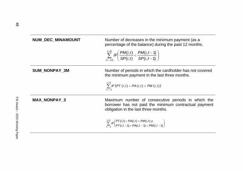
NUM_DEC_MINAMOUNT Number of decreases in the minimum payment (as a percentage of the balance) during the past 12 months.

0

11 )1,(

)1,(

),(

),(t

t tiSP

tiPM

tiSP

tiPMIF

SUM_NONPAY_3M Number of periods in which the cardholder has not covered the minimum payment in the last three months.

0

2

),(),(),(t

t

tiPMtiPAtiPTIF

MAX_NONPAY_3 Maximum number of consecutive periods in which the borrower has not paid the minimum contractual payment obligation in the last three months.

0

2 )1,()1,()1,(

),(),(),(t

t tiPMtiPAtiPT

ytiPMtiPAtiPTIF

NONPAY_SA: Current Non-Payment (ACT)

Number of consecutive periods, up to the reference point, in which the cardholder has not paid its minimum contractual payment obligation.

0

11 )1,()1,()1,(

),(),(),(t

t tiPMtiPAtiPT

ytiPMtiPAtiPTIF

NONPAY_HIS: Historical Non-Payment (HIS)

Number of periods in which the cardholder has not covered the minimum payment in the last six months.

0

5

),(),(),(t

t

tiPMtiPAtiPTIF

NONPAY_HIS_12 Number of periods in which the cardholder has not covered the minimum payment in the last 12 months.

0

11

),(),(),(t

t

tiPMtiPAtiPTIF

FS

I Aw


aper 49

50

FS

I Aw


aper

INC_NONPAY_12M Maximum number of consecutive periods in which the borrower did not make the minimum payment required on the last 12 months.

0

111)____(

t

ttt TSANONPAYTSANONPAYIF

PER_MORE1MIN_12M Number of periods in which the borrower has accumulated over a period without making the minimum payment in the last 12 months.

0

11 )1,()1,()1,(

),(),(),(t

t tiPMtiPAtiPT

ytiPMtiPAtiPTIF

TIMES2NONPAY Number of times that the borrower did not make the minimum payment on two consecutive periods in the past 12 months.

0

11

t

t

IF2)t(i,PM2)t(i,PA2)t(i,PT

and1)t(i,PM1)t(i,PA1)t(i,PT

andt)(i,PMt)(i,PAt)(i,PT

USE_LINE_T0: Credit Limit Use Total outstanding balance as a proportion of the credit limit at the reference point.

),(

),(

tiLC

tiSP

FS

I Aw


aper 51

52

FS

I Aw


aper

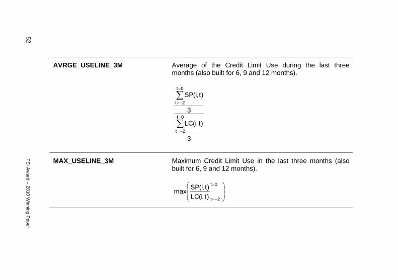
AVRGE_USELINE_3M Average of the Credit Limit Use during the last three months (also built for 6, 9 and 12 months).

3

)t,i(LC

3

)t,i(SP

0t

2t

0t

2t

MAX_USELINE_3M Maximum Credit Limit Use in the last three months (also built for 6, 9 and 12 months).

0t

2t)t,i(LC

)t,i(SPmax

MAXINC_LIMIT Maximum increase in the credit limit during the last 12 months expressed as a percentage of the credit limit in the reference date.

)0.(

)|),(max( 011

iLC

tiSP tt

PGE_OVERLIMIT_3M Percentage of periods in which the borrower over-limit within the last three months (also built for 6, 9 and 12 months).

3

)),(),((0

2

t

t

tiLCtiSPIF

FS

I Aw


aper 53

54

FS

I Aw


aper

PGE_ACTMAX_3M Percentage that represents the balance on the reference date from the maximum balance due in the last three months.

0

2),(max

)0,(t

ttiSP

tiSP

NUM_MAXBALANCE_6M Number of times that the balance was equal to the credit limit in the last six months.

)),(),((0

5

t

t

tiLCtiSPIF

PGE_ENDEBT_6M Percentage that represents the balance on the date of reference against the average balance of the last six months.

6

),(

)0,(1

6

t

t

tiSP

tiSP

PJE_ENDEU_1TRIM Percentage that represents the balance on the last trimester against the average balance of the second trimester.

3

),(

3

),(

3

5

0

2

t

t

t

t

tiSP

tiSP

FS

I Aw


aper 55

56

FS

I Aw


aper

INC_CONSEC_3M Number of consecutive increases in the balance during the last three months.

0

2

))1,(),((t

t

tiLCtiLCIF

DEC_CONSEC_3M Number of consecutive decreases in the balance during the last three months.

0

2

))1,(),((t

t

tiLCtiLCIF

INACUM_T0 Number of cumulative increases in the balance over the past 12 months.

0

11

)1,(),(t

t

tiLCtiLC

DECACUM_T0 Number of cumulative decreases in the balance during the past 12 months.

0

11

)1,(),(t

t

tiLCtiLC

TEOMAT_T0 Theoretical term (months) in which the borrower would cover the total debt according to the minimum payment and the interest rate.

12)0,(

1ln

)0,(*12

)0,()0,(

)0,(ln

iTI

iSPiTI

iPM

iPM

FS

I Aw


aper 57

58

FS

I Aw


aper

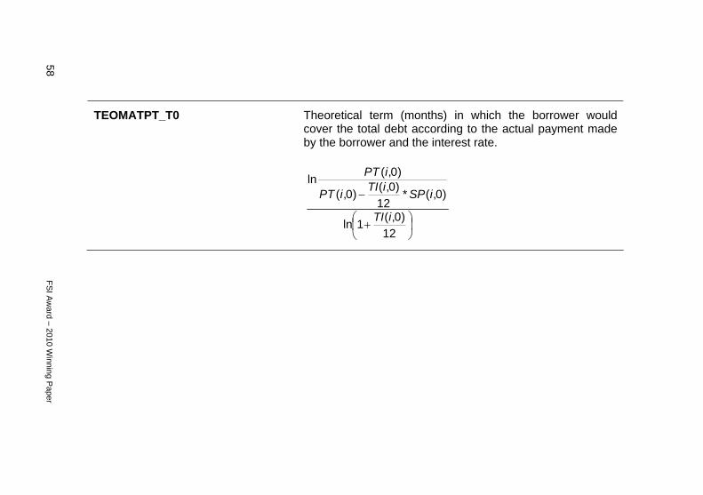
TEOMATPT_T0 Theoretical term (months) in which the borrower would cover the total debt according to the actual payment made by the borrower and the interest rate.

12)0,(

1ln

)0,(*12

)0,()0,(

)0,(ln

iTI

iSPiTI

iPT

iPT

Credit Bureau Information

FS

I Aw


aper 59

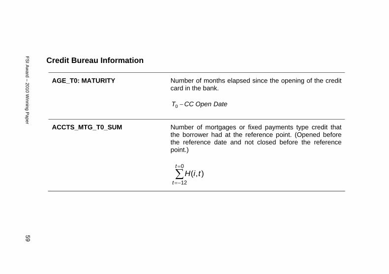
AGE_T0: MATURITY Number of months elapsed since the opening of the credit card in the bank.

DateOpenCCT 0

ACCTS_MTG_T0_SUM Number of mortgages or fixed payments type credit that the borrower had at the reference point. (Opened before the reference date and not closed before the reference point.)

0

12

),(t

t

tiH

60

FS

I Aw


aper

ACCTS_REV_T0_SUM Number of revolving accounts that the borrower had at the reference point. (Opened before the reference date and not closed before the reference point.)

0

12

),(t

t

tiR

ACCTS_TOT_T0_SUM Number of accounts that the borrower had at the reference point. (Opened before the reference date and not closed before the reference point.)

0

12

),(),(t

t

tiRtiH

MTG_T0_SUM Number of mortgages at the reference point.

0

0

),(t

t

tiH

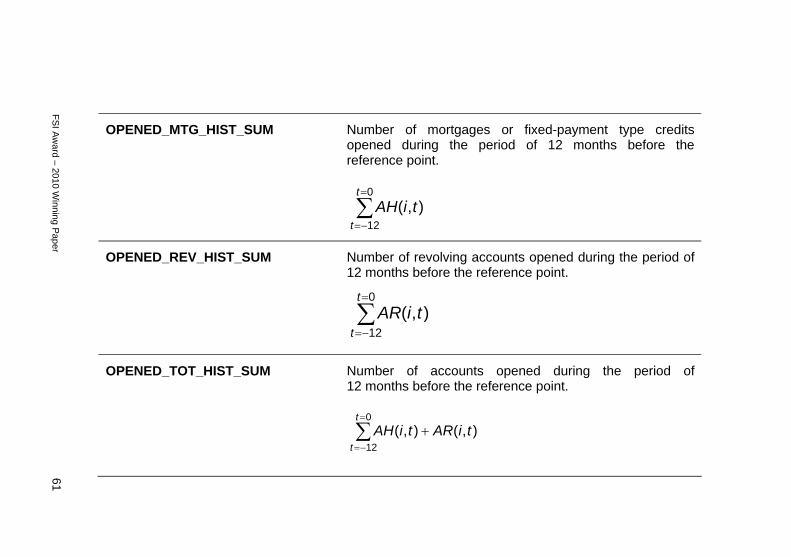
OPENED_MTG_HIST_SUM Number of mortgages or fixed-payment type credits opened during the period of 12 months before the reference point.

0

12

),(t

t

tiAH

OPENED_REV_HIST_SUM Number of revolving accounts opened during the period of 12 months before the reference point.

0

12

),(t

t

tiAR

OPENED_TOT_HIST_SUM Number of accounts opened during the period of 12 months before the reference point.

0

12

),(),(t

t

tiARtiAH

FS

I Aw


aper 61

62

FS

I Aw


aper

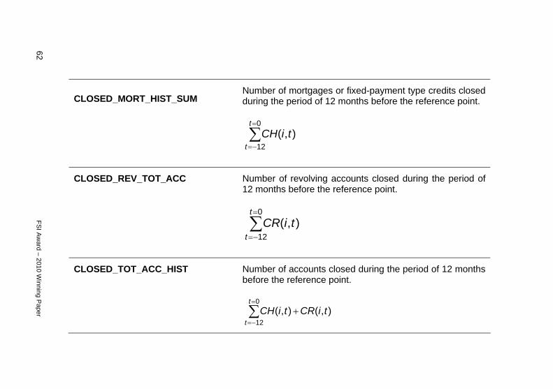
CLOSED_MORT_HIST_SUM Number of mortgages or fixed-payment type credits closed during the period of 12 months before the reference point.

0

12

),(t

t

tiCH

CLOSED_REV_TOT_ACC Number of revolving accounts closed during the period of 12 months before the reference point.

0

12

),(t

t

tiCR

CLOSED_TOT_ACC_HIST Number of accounts closed during the period of 12 months before the reference point.

0

12

),(),(t

t

tiCRtiCH

AGE_BUREAU_T0 Number of months elapsed since the borrower opened his/her first credit in the financial system to the reference point. Months since the first appearance in the Credit Bureau.

CBatcreditfirstofDateT 0

PAST_DUE_HIST Indicates if an account was past due during the period of 12 months before the reference point.

)0,1),,(),(),(( tiPMtiPAtiPTSI

FS

I Aw


aper 63

64

FS

I Aw


aper

Employment Behaviour

INCOME_LVL_T0 Income level at the date of reference.

)0( tSM

AVG_INCOME_6M Income average on the last six months..

6

),(0

5

t

t

tiSM

DAYS_PER_T0 Number of days that the borrower worked in the last two-month period since the reference point.

)0( tDC

FS

I Aw


aper 65

AVG_DAYS_6M Average over the last six months of the number of days the borrower worked in a two-month period.

6

),(0

5

t

t

tiDC

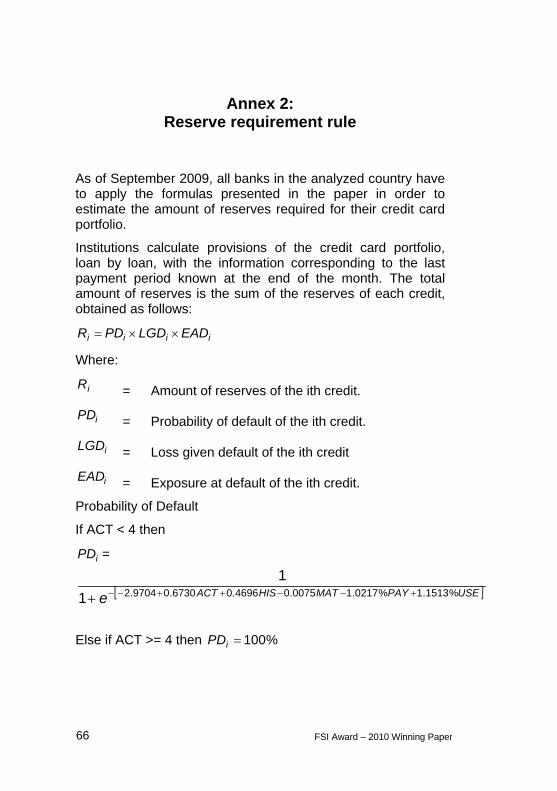
Annex 2: Reserve requirement rule

As of September 2009, all banks in the analyzed country have to apply the formulas presented in the paper in order to estimate the amount of reserves required for their credit card portfolio.

Institutions calculate provisions of the credit card portfolio, loan by loan, with the information corresponding to the last payment period known at the end of the month. The total amount of reserves is the sum of the reserves of each credit, obtained as follows:

iiii EADLGDPDR

Where:

iR = Amount of reserves of the ith credit.

iPD = Probability of default of the ith credit.

iLGD = Loss given default of the ith credit

iEAD = Exposure at default of the ith credit.

Probability of Default

If ACT < 4 then

iPD =

USEPAYMATHISACTe1 %1513.1%0217.10075.04696.06730.09704.2

1

Else if ACT >= 4 then %100iPD


Where:

ACT = Number of consecutive periods, up to the reference point, in which the cardholder has not covered the minimum payment.

HIS = Number of periods in which the cardholder has not covered the minimum payment in the last six months.

MAT = Maturity, measured in months, of the credit card in the bank at the reference point

%PAY = Amount of payment made by the cardholder over the outstanding balance at the reference point

%USE = Percentage that represents the outstanding balance of the credit card at the reference point of the credit limit.

Loss Given Default

If ACT < 10 then %81iLGD

If ACT > 10 then %100iLGD

Exposure at Default

%100,*5784.0

0

00

t

tti CrLimit

BalMaxBalEAD


Where:

Bal = Amount of outstanding balance at the end of the month. For purposes of calculation of Exposure at Default, the variable Bal will take the value of zero when the balance at the end of the month is less than zero.

CrLimit Credit limit authorized for the credit card at the end of the month.

In the case of restructured loans, the institution must keep the borrower's payment history (HIS, MAT) according to the required historical information of the variables.



Bibliography

Basel Committee on Banking Supervision (2000), Strengthening the resilience of the banking sector – consultative document, December.

Basel Committee on Banking Supervision (2006), Basel II: International Convergence of Capital Measurement and Capital Standards: A Revised Framework, June.

Basel Committee on Banking Supervision (2005), An Explanatory Note on the Basel II IRB Risk Weight Functions, July.

Caruana, J. (2010), Systemic risk: how to deal with it? BIS paper, February.

Engelmann, B and R. Rauhmeier, (2006) The Basel II Risk Parameters: Estimation, Validation, and Stress Testing, New York.

Hosmer, David W, Lemeshow, Stanley, (2000) Applied Logistic Regression, Second Edition.

International Accounting Standards Board (2009) Financial Instruments: Amortised Cost and Impairment, Basis for conclusion exposure draft ED/2009/12, November.

Segoviano, M., C. Goodhart (2009), Bank stability measures, IMF WP 09/04, Forthcoming Journal of Financial Stability.

http://www.amazon.com/s/ref=ntt_athr_dp_sr_1?_encoding=UTF8&sort=relevancerank&search-alias=books&field-author=Bernd%20Engelmann

Documents

Regulatory use of system-wide estimations of PD, LGD and EAD - BIS