Regulatory Risk

A paper prepared for the ACCC Regulation and Investment Conference, Manly, 26-27March 2001.

by

Henry Ergas, Jeremy Hornby, Iain Little and John Small

Network Economics Consulting Group*

Abstract

Assets with a value of over $130billion are regulated in Australia. We define regulatory risk

as being regulation that increases the cost of servicing this capital and analyse the sources of

this risk. We show that unbiased and symmetric errors will generally create asymmetric risk

for the firm, that investors cannot fully diversify against this risk, and that the CAPM beta

may even fall when it occurs. The paper concludes with recommendations aimed at

reducing regulatory risk.

* Helpful comments by Jerry Bowman and Walid El-Khoury are gratefully acknowledged.

1 Introduction

When government agencies administer controls over the commercial activities of privatefirms, capital invested in those firms is exposed to an additional source of risk. Because thenature of these controls varies across industries and regulators, the resulting “regulatoryrisk” has many different forms and consequences. One consequence of this diversity ofcauses and effects is that the nature of regulatory risk is not well understood. This in turnlimits the extent to which the costs of regulatory risk can be estimated, and measures can bedesigned to minimise these costs.

This paper begins by presenting some empirical evidence on the size of the regulated sectorin Australia. We use these data to consider both the current costs of regulatory risk and itspossible impacts on investment patterns. This section simply demonstrates that the scale ofthe impact of regulatory risk is very significant.

We then proceed to a more formal analysis, beginning with a definition of regulatory risk.Our definition is presented in section three and centres on the cost of attracting andretaining capital in the firm. Increases in this cost that are caused by regulation are definedas regulatory risk. We discuss the main sources of this risk, which include the length of theregulatory period, the amount of discretion accorded to the regulator, and thediversifiability of the resulting risk. In addition, we show how symmetric errors in settingthe parameters of regulatory models induce outcomes for the regulated firm that are ingeneral asymmetric.

In section four, we characterise the firm’s information about regulatory preferences using asimple model of learning and signalling. The firm needs to form expectations about theoutcomes from future regulatory decisions, and each decision results in an updating of theseexpectations. Using this framework, we are able to derive some qualitative predictionsabout the impact of this type of informational asymmetry. These point to the need forregulators to strive for consistent decision making and also suggest that regulatory riskcould be lower in regimes where regulators have long tenure and wide jurisdiction, sincethese enhance both accountability and credibility.

Section five builds on this analysis by considering the impact of regulatory risk oninvestment. Two subsections address the decisions of portfolio investors, and the realinvestment analysis performed within individual firms. We use a simulation model andtheoretical analysis to demonstrate the perverse predictions that arise from the frequentlyused capital asset pricing model in the presence of regulation. In respect of real investment,our analysis uses a real options framework and concludes that unpredictable regulation willgenerally deter investment.

The paper concludes with some thoughts about the extent to which some regulatory risk isinevitable, and positive suggestions about how unnecessary risk can be reduced withoutcompromising other regulatory goals. These focus on the need for increased levels ofcredibility and accountability by regulators. We argue that increasing the scope and tenureof regulators may help them to develop multi-sector credibility and increase their sense ofaccountability for long-term performance.

2 The Scope of the Problem

Assets with a value of over $130billion are regulated in Australia, either under the terms ofthe Competition Policy Agreement or of statutory instruments (such as Part XIC of the TradePractices Act) that share some similarities with that Agreement. The distribution of theseassets across regulated industries is shown in Figure 1 for the 1998-99 year,1 but these dataexclude some assets (mainly water) for which data is not available.

Figure 1 also provides an indicative estimate of the associated capital related costs.Assuming a simple WACC of 10% and using straight line depreciation based on standardregulatory practice/decisions, we estimate that capital related costs are around $18 billionper annum. This is approximately 3% of GDP per annum. If regulatory risk were toincrease the rental cost of this capital by 1%, total costs would rise by $180million perannum.

Apart from affecting the annual costs of funding assets that are currently sunk intoregulated industries, the biggest danger of regulatory risk is that it can choke off otherwisedesirable investment in new technologies and equipment. We explain below that a keydeterrent of investment is the difference between typical asset lifetimes and the span ofregulatory cycles. Figure 2 sets out, for each of the major regulated industries, the asset lifeof the predominant asset and compares this with the regulatory cycle. It shows that for mostindustries, the major asset has an asset life in excess of 8 times the standard regulatoryperiod. As a result of this gap between asset lives and regulatory cycles, investors in theseindustries cannot secure a high degree of commitment, from regulatory authorities, aboutthe manner in which the returns on long-lived assets will be determined.

1 This data was sourced from regulatory decisions, annual reports and the Productivity Commissionreport Financial Performance of Government Trading Enterprises 1994-95 to 1998-99 - Performance MonitoringReport

Figure 1: Value of regulated utility sector 1998-99

Regulated industry

Indicative regulated asset

base ($bn)

Indicative economic asset

life

Annual depreciation based on indicative asset

life ($m)

Return on capital -10% WACC ($m)

Electricity 32 20 1,600 3,200 Gas 13 50 260 1,300 Water 39 70 557 3,900 Telecoms 28 12 2,333 2,800 Rail 16 40 400 1,600 Ports 3 30 100 300 Airports 3 30 100 300 Total/average 134 5,350 13,400

Long asset lives are reflected in high average ages for the capital stock. The following figureshows the average age of the capital stock across a range of industries, and is notable for therelatively old capital being used in the regulated electricity gas and water sectors. Even intelecommunications, where technological progress is rapid, the capital stock is more than 10years old on average.

High average ages of the capital stock may partly reflect relatively slow demand growth,though this is not apparent from the results of correcting for the growth rate of the netcapital stock. Additionally, in some regulated industries, there may be an overhang of excesscapacity resulting from uncommercial investments carried out under public ownership.Nonetheless, it is also likely that the industries at issue will face considerable investmentdemands in the medium-term, as now rather old assets come up for replacement. As aresult, an increase in the cost of capital due to unnecessary regulatory risk could impose asignificant burden on the community.

Figure 2: Relationship between asset life and regulatory cycle

Regulated industry Major assetEconomic life

major asset

Typical regulatory

cycle

Ratio economic life to

regulatory cycle

Electricity Poles 45-55 5 9-11Gas Pipelines 80 5 20Water Mains 70-90 3-5 14-23Telecoms Copper pair 20 ad hoc/3 7+Rail Track 40 5 8Ports Channel improvements 30+ 5 6+Airports Runway (ave) 30-40 3-5 8-10

Figure 3: Average age of capital stock

0.00

5.00

10.00

15.00

20.00

25.00

Elec

tric

ity, g

asan

d w

ater

Tran

spor

t and

stor

age

Com

mun

icat

ion

Acc

omm

odat

ion,

cafe

s an

dA

gric

ultu

re,

fore

stry

and

Con

stru

ctio

n

Cul

tura

l and

recr

eatio

nal

Fina

nce

and

insu

ranc

e

Min

ing

Man

ufac

turi

ng

Ow

ners

hip

ofdw

ellin

gsPe

rson

al a

ndot

her

serv

ices

Prop

erty

and

busi

ness

ser

vice

s

Ret

ail t

rade

Who

lesa

le tr

ade

Average 1997-2000 (adjusted for net capital growth)

Average 1997-2000

All industries (adjusted for net capital growth)

All industries

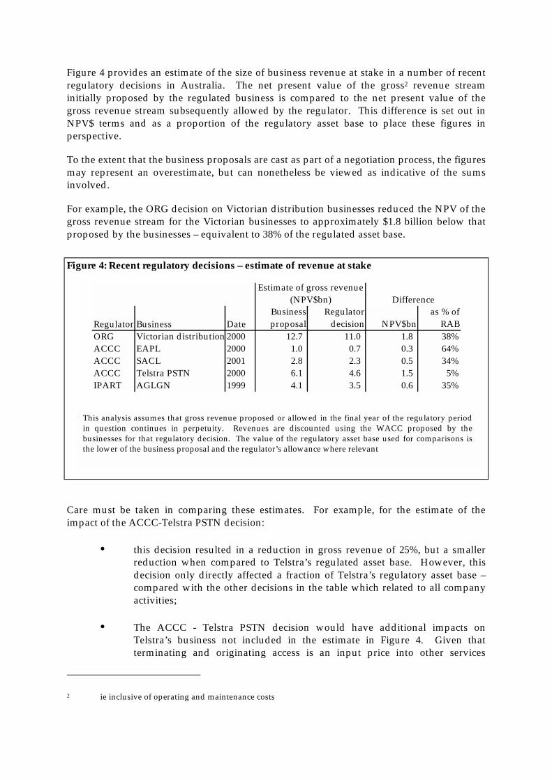
Figure 4 provides an estimate of the size of business revenue at stake in a number of recentregulatory decisions in Australia. The net present value of the gross2 revenue streaminitially proposed by the regulated business is compared to the net present value of thegross revenue stream subsequently allowed by the regulator. This difference is set out inNPV$ terms and as a proportion of the regulatory asset base to place these figures inperspective.

To the extent that the business proposals are cast as part of a negotiation process, the figuresmay represent an overestimate, but can nonetheless be viewed as indicative of the sumsinvolved.

For example, the ORG decision on Victorian distribution businesses reduced the NPV of thegross revenue stream for the Victorian businesses to approximately $1.8 billion below thatproposed by the businesses – equivalent to 38% of the regulated asset base.

Care must be taken in comparing these estimates. For example, for the estimate of theimpact of the ACCC-Telstra PSTN decision:

• this decision resulted in a reduction in gross revenue of 25%, but a smallerreduction when compared to Telstra’s regulated asset base. However, thisdecision only directly affected a fraction of Telstra’s regulatory asset base –compared with the other decisions in the table which related to all companyactivities;

• The ACCC - Telstra PSTN decision would have additional impacts onTelstra’s business not included in the estimate in Figure 4. Given thatterminating and originating access is an input price into other services

2 ie inclusive of operating and maintenance costs

Figure 4: Recent regulatory decisions – estimate of revenue at stake

Regulator Business DateBusiness proposal

Regulator decision NPV$bn

as % of RAB

ORG Victorian distribution 2000 12.7 11.0 1.8 38%ACCC EAPL 2000 1.0 0.7 0.3 64%ACCC SACL 2001 2.8 2.3 0.5 34%ACCC Telstra PSTN 2000 6.1 4.6 1.5 5%IPART AGLGN 1999 4.1 3.5 0.6 35%

Estimate of gross revenue (NPV$bn) Difference

This analysis assumes that gross revenue proposed or allowed in the final year of the regulatory periodin question continues in perpetuity. Revenues are discounted using the WACC proposed by thebusinesses for that regulatory decision. The value of the regulatory asset base used for comparisons isthe lower of the business proposal and the regulator’s allowance where relevant

provided by Telstra – namely STD and IDD - this decision would havereduced the prices Telstra would be able to charge in these markets. Giventhat these markets are competitive, and that any reduction in input priceswould be passed on to consumers, it is estimated that the overall effect of theACCC’s decision would be to reduce Telstra’s revenue (in NPV terms) by$2.8bn from Telstra’s initial proposal – a reduction in gross revenuecomparable to 10% of its regulatory asset base.

For the decisions outlined above, Figure 5 provides an estimate of the major factorsaccounting for the differences in the two revenue streams3. The predominant factor in allthese decisions is the importance of the regulator’s decision on the return on asset – whichreflects decisions with respect to asset valuation and WACC. The importance of thesefactors is disproportional to their respective importance in the annual revenue requirement.This is not unexpected, particularly in decisions where the value of the asset base is subjectto review (eg SACL, EAPL).

Overall, these estimates highlight both the extent of the impact regulatory decisions canhave and the range and significance of the economic activity thereby affected. Betterunderstanding and managing the risks regulation can create is therefore likely to be ofsubstantial importance.

3 Definition and taxonomy of regulatory risk

We define regulatory risk through its effect on regulated firms. Regulatory risk arises whenthe interaction of uncertainty and regulation changes the cost of financing the operations ofa firm. This definition is broad enough to include all of the important sources ofuncertainty, but restricted to those for which the effect on the firm arises from, or ismagnified by, the existence of regulation. Further, it excludes changes that induce windfall

3 These figures should be considered as indicative as the variables included in the table are notnecessarily mutually exclusive

Figure 5: Factors accounting for difference in revenue stream (%)

Regulator BusinessReturn on capital

Depreciation O&M

ORG Victorian distribution 81% -13% 31%ACCC EAPL 63% 37% 0%ACCC SACL 75% 13% 12%ACCC Telstra PSTN 100% 0% 0%IPART AGLGN 36% 30% 34%

Average of these decisions 80% 3% 17%

capital gains and losses except to the extent that such changes also affect the discount ratesof investors.4

An important advantage of this focus on discount rates is that it links the impact of risk onportfolio investors with decisions made within the firm over real investment opportunities.If a real investment project is to be undertaken, it is necessary, though not always sufficient,5that it be expected to cover the cost of capital.

Our definition imposes no particular “sign” on the effect of regulatory risk, so it is alsopossible for such risk to reduce the discount rate of a firm. For example, an increase in thelevel of regulatory risk faced by a firm subject to direct regulation, may lead investors toalter their portfolios in favour of some other firm (this is demonstrated below using asimulation study). An important question to be addressed below concerns the impact ofsuch a shift on the distribution of capital costs across firms.

3.1 Types of uncertainty

Regulatory risk cannot arise without uncertainty, and it is useful to distinguish two broadcategories of uncertainty. We define “market uncertainty” as being that which wouldremain if all relevant regulatory interventions ceased. Market uncertainty arises from thenormal stochastic interaction between buyers and sellers across all markets. This includesthe impact of external cost shocks, unanticipated technological advances, shifts inpreferences, changes in the distribution of income across people, and changes in thedistribution of people across regions.

Although the effects of market uncertainty are felt by all firms, irrespective of whether theyare regulated or not, this does not make market uncertainty irrelevant in the assessment ofregulatory risk. On the contrary, because this wider market uncertainty represents thealternative opportunities available to portfolio investors, the interaction between it and thereturns required by investors in regulated assets is crucial to determining the effect ofregulatory risk.

The second type of uncertainty arises from the existence of regulatory discretion. One of themost fundamental reasons for addressing competition issues through regulation rather thanthrough legislation is that a complete set of rules is very difficult (if not impossible) tospecify in advance, and the costs of adapting pre-specified rules to changing circumstancesthrough legislative amendment are considered to be greater than those of relying onregulatory decisions made within the terms of more open-ended standards.6 Thus,

4 This could be achieved by a regulator who is about to be retire. If everyone knows that a new personwill be responsible for policy in the future, and believed that the probability of a second value cut wasextremely low, then the cost of capital might not increase appreciably.

5 Real options, which may increase the “hurdle rate” for projects beyond the cost of capital, are discussedin more depth below.

6 See especially D. J. Galligan (1986) Discretionary Powers: A Legal Study of Official Discretion, Oxford,who defines “discretion” as the power to take a decision when there is no pre-defined “right” answer(at page 7) or more precisely as the consequence of “an express grant of power conferred on officialswhere determination of the standards according to which power is to be exercised is left largely tothem”. In a famous analogy, the eminent legal theorist Ronald Dworkin has described discretion interms of a doughnut – where discretion is the hole in the middle, while the doughnut itself constitutes

regulators always have some non-trivial decisions to make. As a consequence, the outcomesfrom the future stream of regulatory decision making processes cannot be predicted withcertainty. We refer to this as “regulatory uncertainty” because it is a direct consequence ofregulatory discretion.

Regulatory risk is the expected cost of the interaction of regulatory controls with uncertaintyof both types. Thus, a high level classification of uncertainty types does not provide acomplete taxonomy of the sources of regulatory risk. We propose such a classification in thenext section.

3.2 Sources of regulatory risk

Market uncertainty is the constant companion of all commercial activity, whereas regulatoryuncertainty only exists for those activities that are actively controlled by a regulator in someway. It is possible to impose regulations without allowing any regulatory discretion,however, and in this case there is no regulatory uncertainty. Accordingly, we consider twoprimary sources of regulatory risk, which are distinguished by the presence or absence ofregulatory discretion.

3.2.1 Certain regulation

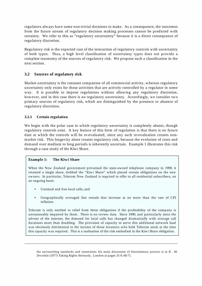
We begin with the polar case in which regulatory uncertainty is completely absent, thoughregulatory controls exist. A key feature of this form of regulation is that there is no futuredate at which the controls will be re-evaluated, since any such re-evaluation creates non-market risk. This longevity alone creates regulatory risk, because the evolution of costs anddemand over medium to long periods is inherently uncertain. Example 1 illustrates this riskthrough a case study of the Kiwi Share.

Example 1: The Kiwi Share

When the New Zealand government privatised the state-owned telephone company in 1990, itretained a single share, dubbed the “Kiwi Share” which placed certain obligations on the newowners. In particular, Telecom New Zealand is required to offer to all residential subscribers, onan ongoing basis:

• Untimed and free local calls; and

• Geographically averaged line rentals that increase at no more than the rate of CPIinflation.

Telecom is only entitled to relief from these obligations if the profitability of the company isunreasonably impaired by them. There is no review date. Since 1990, and particularly since theadvent of the internet, the demand for local calls has changed dramatically with average calldurations more than doubling. The provision of capacity to serve this additional network loadwas obviously detrimental to the income of those investors who held Telecom stock at the timethis capacity was required. This is a realisation of the risk embodied in the Kiwi Share obligation.

the surrounding standards and constraints: his main discussion of discretionary powers is in R . M.Dworkin (1977) Taking Rights Seriously, London at pages 31-9, 68-71.

3.2.2 Uncertain regulation

When controls are administered by an active regulator, additional sources of risk arise fromthe fact that the future decisions of that regulator (and his successors) are not fullypredictable. Any particular decision by the regulator will affect the payoff to the regulatedfirm, and its rivals. While individual decisions are therefore important to investors, it is thebeliefs of investors about the future distribution of returns that feeds into the calculation ofregulatory risk.7

Three factors directly effect the cost of regulatory risk. These are: the frequency of decisionpoints; the level of discretion available at each decision point; and the diversifiability of theresulting risk. We discuss each of these in turn.

3.2.3 Frequency of decisions

Regulatory risk only arises in the presence of sunk costs. If no funds have been committedto long-lived assets, any regulatory decision that prevents the firm from covering its averagecosts will simply provoke immediate exit from the market. There would be no increase infuture costs, unless a perverse regulatory outcome drove out relatively low cost suppliers.

Similarly, if long-lived assets are required to provide the regulated service, a regulatorycontract of similar duration could eliminate this component of regulatory risk in respect ofthose assets. It is only when the terms of the (usually at least partly implicit) regulatorycontract are able to be re-set before the end of the life of the relevant assets, that regulatoryrisk arises. In this case, regulatory risk increases with the frequency of the re-set dates.

3.2.4 Level of Discretion

If the regulator is required by law to follow an exact and complete set of rules when makingdecisions, non-market risk would be eliminated. This is generally not feasible, however, andregulators typically do have considerable freedom to make determinations that affect thepayoff to the firm.

Even limited and incomplete regulatory rules can reduce the risk arising from discretionarypowers, however. For example, suppose that the regulator is given the right to require thefirm to invest or not invest in particular projects. This creates significant discretionarypower but may not lead to a reduction in the value of the firm if the regulator is alsorequired to ensure that the firm continues to earn a specified rate of return on capital.

Firms need to form expectations about the outcome of future regulatory decisions in order toevaluate the business case for investment projects. In forming these expectations, the firmwill look to any past history of regulatory decision-making by the same people, and willupdate these expectations each time a new decision is observed. This learning processimplies that regulatory uncertainty is highest, early in the tenure of a new regulator.

7 Investors’ beliefs about the future distribution of returns, when combined with information on thereturns available from alternative stocks, determine the cost to the firm of retaining financial support.Because our definition of regulatory risk is focussed on the cost of capital, the interaction betweenanticipated distributions of returns from the regulated firm and the market portfolio is central to thisanalysis.

3.2.5 Diversifiability of Risk

The incidence of regulatory risk is also relevant when considering the cost of this risk, fortwo reasons. First, the social cost of risk depends on its incidence, and will be minimised byallocating regulatory risk to those best equipped to deal with it. Secondly, the incidence ofregulatory risk also affects its cost to investors, who have the ability to diversify some typesof risk across a market portfolio. We address the diversifiability of regulatory risk further insection 4 below.

3.3 Estimation Error Effects

Regulators operate without full information about the regulated firm, and must thereforeestimate the relevant parameters, such as the WACC. Any given determination of aregulator is therefore likely to include some estimation error. In this section we show thateven if there is no bias in the regulator’s estimation (so that the expected value of eachparameter estimate is equal to the true parameter), the consequences of such errors areasymmetric, to the detriment of the firm’s income. This result only relies on very weakassumptions about the properties of cost and revenue functions.

The economic profit of the firm can be written as follows:

Π(p) = R(p) – C(p)

where R(p) is the revenue function, C(p) is the cost function and p is the vector of prices.Under very general conditions, the revenue function is concave and the cost function isconvex, so the profit function is concave in prices.8 The regulator controls the firm’s prices,either implicitly (for example by specifying a rate of return) or explicitly (as in a price cap),and thereby prevents the firm from optimising against the demand curve. The firm retainsthe ability to minimise production costs, though the minimum cost function is fixed in theshort run.

Suppose for concreteness that the regulator attempts to set the price directly at the level thatis consistent with the firm making zero economic profits. Let pR be the price that achievesthis goal exactly, so that Π(pR)=0, and consider the effect of estimation error that results in amean-preserving spread around pR. For example, suppose that instead of correctlyestimating pR, the regulator instead sets pH = pR + δ or pL = pR - δ, with equal probability.Over many estimates the regulator is correct on average, but any single estimate is alwayswrong. Although the average regulatory error is zero, the average consequence is aneconomic loss. This result derives exclusively from the concavity of the profit function.Using the definition in footnote 4 with α = ½, this concavity implies that

Π(½pL + ½pH) > ½Π(pL) + ½Π(pH)

Since pR = ½pL + ½pH by construction, we can rewrite this as

Π(pR) > ½Π(pL) + ½Π(pH)

Recall that pR was defined to ensure that Π(pR)=0. Thus

8 If f(x) is concave, then for any α (where 0 ≤ α ≤ 1), f(αx’ + (1-α)x’’) > αf(x’) + (1-α)f(x’’).

0 > ½Π(pL) + ½Π(pH)

which says that the firm makes a loss, even when the regulator estimates pR correctly onaverage. This result is nothing more than an application of Jensen’s Inequality9 to the(concave) profit function of a regulated firm.

3.3.1 Compensation for unbiased error

Because the loss arising from unbiased regulatory error is directly related to the curvature ofthe regulated firm’s profit function, it is theoretically possible to estimate the size of the loss.To do so, we need to combine the probability distribution of the estimation errors with thefirm’s profit function. The following diagram, which is based on a uniform distribution oferrors, illustrates the idea.

The diagram shows a simple case in which the firm charges linear prices (i.e. without fixedmonthly charges or price discrimination), and the regulator estimates the regulated pricethat gives zero economic profit pR imperfectly, selecting pH and pL with equal probability,where these are as defined above. Concentrating on the difference between the profitarising from pH and the loss from pL, allows us to ignore the large surplus rectangles qH(pH –pR) and qH(pR - pL), these being of equal size. The expected profit difference from this formof regulation is the difference in the area between the demand curve and the average costcurve over the region from qR to qH (which is the “upside” from a positive error) and overthe region from qR to qL (which is the “downside” from a negative error). If the average costfunction is convex, the downside is greater than the upside.

If we define the demand and cost properties as functions of the output level q, so demand isp(q) and cost if C(q), we can estimate the loss arising from random error as:

9 Jensen, J.L.W.V. (1906) “Sur les fonctions convexes et les inegaites entre les valeurs moyennes” ActuarialMathematics, 30, pp. 175-193.

( ) ( )∫∫ −−−=R

H

L

R

q

q

q

qdq)q(C)q(pdq)q(p)q(CL

The first term on the right hand side is the the loss arising from setting the price at pL andthe second term is the profit from setting the price at pH.

3.3.2 Non linear pricing

Many utilities set two-part tariffs, comprised of a monthly fixed fee plus a usage sensitivecharge, rather than a simple linear price. If this type of tariff structure materially affects thecurvature of the profit function, it will also change the amount of compensation required.While a complete analysis of this issue is beyond the scope of the present paper, two pointsare relevant.

First, more sophisticated tariff structures will not alter the fact that the revenue function isconcave. This follows from the very weak proposition that there is some limit to the averagemonthly outlays on service that can be achieved.

Secondly, it seems at least plausible that the revenue function will be more concave whennon-linear tariffs are used than when they are not. This is because the firm is able to capturea greater share of the total surplus with non-linear tariffs. Since producer and consumersurplus are both concave functions of feasible output levels, it is at least plausible that theirsum will be more concave than either one individually.

3.3.3 Competitive effects

The above analysis has implicitly considered monopolies, whereas some regulated firmsface competition for the supply of the regulated service. Many incumbenttelecommunications companies, for example, sell network access services at the wholesalelevel to their retail market competitors. In these cases, the asymmetric effect of unbiased (i.e.symmetric) errors in the setting of regulatory parameters is reinforced by competitiveinvestment behaviour.

When the access price is set at pL, renting access is unambiguously preferred to buildinginfrastructure. This follows directly from the facts that pL < pR and Π(pR)=0. When the priceis too high, however, potential access seekers face a non-trivial build/buy decision. Theywill not necessarily build when faced with an access price of pH, because of the impact ofreal options (see below) and the effect of the additional capacity on the earning power of theasset under consideration. However, the fact that the investment decision is non-trivialsuggests that investment will occur in some cases. The resulting decline over the long-termin expected demand for the services of the regulated asset reduces the value of that asset.

This effect reinforces the conclusion that symmetric errors in regulatory price setting haveasymmetric impacts on the regulated firm.

4 Learning and Signalling

Inherent in any regulatory relationship are information asymmetries where the informationknown by one party is not shared with the other. These asymmetries may favour eitherparty. The incentive regulation literature emphasises the case where the regulator is

disadvantaged in not knowing the firm’s inherent efficiency (or “type”). In this section weconsider the reverse case, in which the firm knows less than the regulator about theintentions of the regulator, or more generally, of what type the regulator is.10

Given this uncertainty, the firm must make an assessment of what it expects the regulator’stype to be, in order to forecast its returns on existing and future investments (if a regulationis expected to be heavy-handed then the firm will expect to earn lower regulated returnsthan if the regulation is expected to be light-handed). The firm will construct its expectationusing the information that it possesses, that is, the history of the regulator’s decisions.Consequently, if the regulator has a history of imposing heavy-handed regulations then thefirm will expect future regulations to be more heavy-handed than light.

The regulator, therefore, influences the firm’s expectation of future regulations with itschoice of present regulation. In this sense, current regulation has two roles: the first is theimmediate realisation of social gains; and the second is “signalling” future regulatorysettings to the firm. Because these future settings are key determinants of the return toregulated capital over the medium term, the regulator’s signalling activity has a direct effecton investment. Two attributes of the regulator’s signalling are particularly important:consistency and credibility. We discuss each of these separately.

4.1 Consistency of signals

The strength of the regulator’s signal, which can be measured by the consistency of itsdecisions, influences the degree of regulatory risk faced by the firm. This is best explainedin the following example.

Suppose the decisions of regulators can be classified into types situated along a continuum.At one end is a regulation that will expropriate all the firm’s returns from sunk investments,and at the other end is a regulation that will allow the firm to operate without impediment.

If, in one extreme case, the regulator makes its decisions from a random draw from thecontinuum, its history will provide no guidance to the firm when it constructs itsexpectations of future regulation. The firm will expect that any forthcoming regulations arejust as likely to be heavy-handed as light-handed or anywhere in between. This inability tomake reliable predictions about the regulator’s future decisions adds non-market risk andthereby increases the firm’s exposure to regulatory risk.

Suppose, in the other extreme, the regulator commits to a place near the middle of thecontinuum and, henceforth, all its decisions are consistent with that commitment. Aftersome history of regulation has developed, the firm will soon see that all regulation is of thesame type and will not expect future regulation to deviate very far from its average. In thiscase the reliability of the firm’s expectations is enhanced (relative to the previous case wherethe regulator made decisions randomly), and consequently the regulatory risk faced by thefirm is reduced. This example has shown that the regulator can use signalling to make acommitment to its type, having the direct result of decreasing the regulatory risk that isotherwise imposed on the firm.

10 This section has some parallels with models of regulatory commitment as a game. See for example R.J.Gilbert and D.M. Newbery, 1994, The dynamic efficiency of regulatory constitutions, RAND Journal ofEconomics, 25, 538-54.

4.2 Credibility of signals

The strength of the regulator’s signal is influenced by the credibility of the regulator’scommitment, where “credibility” in this sense refers to the rational and statisticalexpectation of the firm. If a regulator attempts to signal that it will allow a fair return onsunk costs, but has a reputation of expropriating the surplus generated from other sunkcosts, it will find it difficult to convince the firm that is will not act in this way once newfunds have been sunk. The firm will recognise that history is likely to repeat itself and itsfuture investment decisions will reflect this expectation.

If the regulator is able to credibly signal that it intends to allow the firm to recover its sunkcost, then efficient11 investment will be forthcoming. Regulators may be able to build theirown credibility in some ways. The provision of an efficient (e.g. speedy) and consistentregulatory service to the industry would, for example, send a strong and credible signal ofgood intentions. The credibility in this signal derives mainly from the fact that it requiresconsiderable effort on the regulator’s part, effort that would not be expended unless theregulator really understood the value firms place on certainty.

Assuming that the regulator is operating at maximum efficiency, what are the otherconstraints on regulatory credibility? Three questions would seem to be important:

1. How long does it take a firm to forget?

2. Does the firm take notice of the regulator’s activities in other industries?

3. What is the regulator’s tenure?

The answers to these questions are subjective, and can therefore not be determined merelyby logical analysis. We can, however, draw some qualitative conclusions.

In respect of the first question, if the firm places a relatively heavy emphasis on the recentparts of the regulator’s history when constructing an expectation of future regulation thenthe regulator will find it relatively easy to change signals. In this case, the effect of decisionsmade in the distant past will receive relatively small weights in the firm’s decision making.However, if the firm puts equal weight on past decisions then any action by the regulatorthat deviates from its signal will have a longer effect on the investment decisions of firms.

The second question clearly depends on the scope of the regulator’s jurisdiction. Suppose asingle regulator has responsibility for two industries, A and B, and that he has to dateconsistently allowed firms in A to earn fair returns in one industry, but expropriated allreturns in B. In this case, firms in industry A might reasonably expect to be regulated in asimilar way to the later industry in the future. In this case the regulator’s current signal toindustry A lacks credibility because it is inconsistent with his actions in industry B. Example2 demonstrates the relevance of these cross-industry effects.

11 At least with respect to this dimension of the investment decision. Information asymmetries maycompromise the regulator’s ability to elicit the overall efficient level of investment.

Example 2: Victorian gas and electricity regulation

Investors in the Victorian distribution assets, privatised by the Victorian Government in1995, faced uncertainty through the interaction of:

• the creation of an independent economic regulator (the Office of theRegulator General); and

• the specification of a regulatory regime that provided:

! a reasonable degree of certainty in regulatory policy for the firstregulatory period; but

! little guidance as to the regulator’s decisions for subsequentreview periods.

Given that such reform was new in Australia, investors in these utilities had little chanceto learn about the likely actions of the regulator. In addition, the regulator had littleopportunity to signal its intentions.

In this environment, the ORG’s subsequent decision in a related market (gas) can be seennot only as a decision affecting the gas sector, but also as the ORG signalling itsintentions as to its regulatory stance in its (then) forthcoming electricity distribution pricereview, with investors learning about the regulators actions in that review and adjustingexpectations accordingly. A downwards revision in investors expectations appears tohave accompanied the ORG/ACCC’s draft gas decision (May 1998) given that in thethree weeks following this decision, the share prices of electricity distributors UnitedEnergy and AGL fell by 15.7 and 14.2 percent respectively(http://www.ue.com.au/download/hambros.pdf).

This learning impact is also evident by the absence of any discernable shift in the shareprice of both companies following the ORG’s final decision on electricity distribution.

Cross-industry signalling is not possible unless the regulator has cross-industry jurisdiction.In this sense, the pooling of regulatory functions makes it possible to reduce regulatory risk.The mere fact that a regulator has wide jurisdiction does not mean that the resultingpotential for risk reduction will be realised of course. Indeed, society would be far better offwith numerous industry specific regulators all generating strong (i.e. clear) signals abouttheir future behaviour, than with one omnibus regulator behaving erratically.

The third question addresses the issue of accountability. The most important consequenceof regulatory risk is a reduced level of real investment, the effects of which are unlikely to beapparent for several years. If the tenure of regulatory decision makers is sufficiently long,they will be personally required to confront any adverse consequences arising from theirearlier decisions.

5 Investment Effects

As discussed above, regulatory risk influences the expectations of agents about payoffsreceived by the firm across the range of possible market outcomes. These expectations areused in capital allocation decisions at two levels: portfolio investment and real investment.In this section, we describe the effect of regulatory risk on each of these forms of investment.

The strategies of portfolio investors depend on their expectations about the future returnsachievable across the entire range of possible securities. The result of many such investorsoptimising their allocations of capital can be summarised in several ways, the best known ofwhich is the capital asset pricing model, or CAPM. Although this model does not enjoy theunanimous support of financial economists, it is well understood and widely used byregulators and business people alike. For this reason, our analysis of the impact ofregulatory risk on investors, developed in the next sub-section, is based on the CAPM.

Real investment decisions are taken by the managers of firms, rather than a large number ofportfolio investors. Managers are responsible for ensuring that the investment strategy ofthe firm results in the best possible flow of returns to investors. This requires carefulattention to choices over technology, location, scale and timing. In the second subsectionbelow we focus on just one of these choices: that of optimal investment timing.

5.1 Effect on beta

The capital asset pricing model12 (CAPM) provides a method for estimating the riskassociated with investing capital into all of the securities that make up the market portfolio.13

Within the CAPM, risk associated with any given security is only compensated to the extentthat it increases the risk of the market portfolio. This component of risk is referred to as“systematic risk”. The rationale for this restriction is that systematic risk cannot bediversified by holding other securities.

While it is logically correct to argue that investors only require compensation for thosecomponents of risk that cannot be diversified, the systematic risk that is priced within theCAPM is not the only such risk. Firm specific risk which does not contribute to the risk ofthe market portfolio, (i.e. which is not systematic) is not priced by the CAPM, even if itcannot be mitigated by diversification.

5.1.1 Non-diversifiable, non-systematic risk

There are two important types of regulatory risk that are neither systematic nordiversifiable. For expository purposes, it is convenient to think of these as arising from

12 W.F. Sharpe, 1964, Capital Asset Prices: A Theory of Market Equilibrium Under Conditions of Risk,Journal of Finance, 19, 425-42. J. Lintner, 1965, The valuation of risk assets and the selection of riskyinvestments in stock portfolios and capital budgets, Review of Economics and Statistics, 47, 13-37.

13 The market portfolio is the universe of financial securities available to investors. Fully diversifiedinvestors can be thought of as holding a share of the market portfolio, meaning that the proportion ofeach security in the investor’s own portfolio is equal to the weight that secuirty receives in the marketportfolio.

“certain” and “uncertain” regulation respectively, where these terms are as defined insection 2 above.

Consider a long-lived regulation that caps the prices of a monopoly that serves the publicdirectly, at levels that are known by all parties. For concreteness, we could think of this as atwenty-year CPI-X price cap combined with an obligation to serve all demand. Marketconditions evolve stochastically, affecting the strength of demand for the firm’s service andits cost of production. If there were no regulation, the firm would adjust prices to takeadvantage of these varying conditions. Indeed, provided the cost of making theseadjustments were not too large, the stochastic market conditions may enable the firm tomake higher profits than would otherwise be the case.14

The imposition of the price control completely reverses this effect. Now, rather than beingable to optimise in the face of random market conditions, the firm’s role is entirely passive.Its prices are fixed so it has no ability to regulate demand, and its inputs are priced incompetitive markets which are subject to external shocks. Under these conditions, marketrisk is unambiguously harmful to the firm’s expected profitability.15

Paradoxically, the imposition of regulatory controls of this type can reduce the contributionthe affected firm makes to the risk of the market portfolio, thereby reducing the cost ofcapital as predicted by the CAPM.16 When this occurs, the risk induced by certain regulationis not systematic. Equally important, this risk is not readily diversifiable. In the presentexample, the reasons are obvious. The regulated firm is a monopoly that serves the publicdirectly, so no other firm gains when the regulated firm loses. The beneficiaries ofregulation are final consumers, and since investors cannot directly17 purchase claims on theresidual income of final consumers, their ability to avoid this type of risk is limited.18

Investors will require compensation for exposure to risk of this type, but it is not priced bythe CAPM. As a result, when regulators use the CAPM framework to estimate the cost ofcapital, they understate the required return by the amount of fair compensation for non-

14 For an unregulated firm with low adjustment costs, the maximum profit function is convex in prices. Inthis case, Jensen’s inequality implies that profits are higher when prices are random. See RichardHartman (1972), The Effects of Pice and Cost Uncertainty on Investment, Journal of Economic Theory, 5,258-66.

15 This is because the firm cannot maximise against fluctuating demand. The maximum profit that wouldbe earned by an unregulated firm is not available. Under these conditions, the maximum profit functionis identical to the profit function, and hence is concave rather than convex. Jensen’s inequality thereforeimplies that uncertainty will reduce the average profit. This reduction needs to be taken into accountwhen setting regulatory parameters.

16 This is demonstrated by Ergas and Small (1999) “The Rental Cost of Sunk and Regulated Capital”,CRNEC Working Paper 17, University of Auckland (http://www.crnec.auckland.ac.nz)

17 Indirect diversification could be obtained by investing in firms that might enjoy increased businesswhen final consumers are better off.

18 Investors may well hold other stocks regulated by the same authority, and if the transfers betweenregulated firms and consumers were purely random, investors would gain income from those stocksthat receive transfers, offsetting losses on those stocks that pay the transfers. There is still a net loss inthis case, because of the concavity of the profit function.

diversifiable, but non-systematic risk. As discussed further below, this amount can bethought of as an insurance premium.

5.1.2 Simulation study

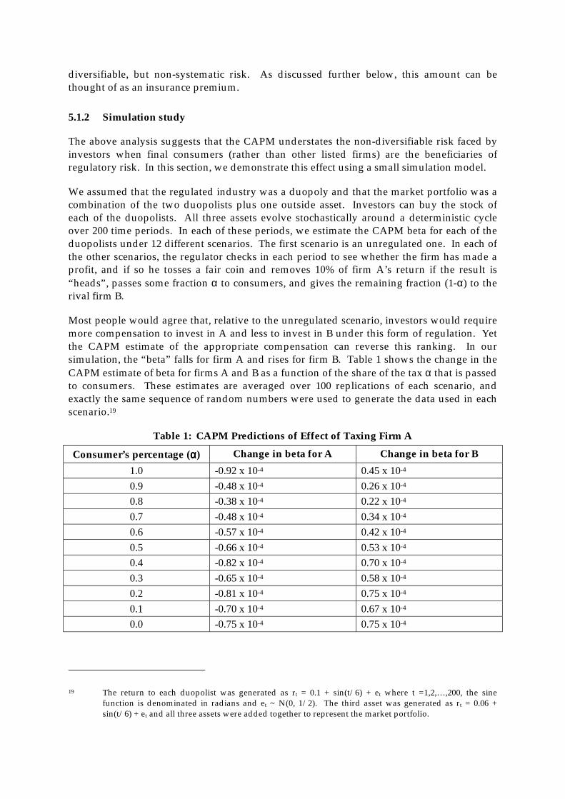
The above analysis suggests that the CAPM understates the non-diversifiable risk faced byinvestors when final consumers (rather than other listed firms) are the beneficiaries ofregulatory risk. In this section, we demonstrate this effect using a small simulation model.

We assumed that the regulated industry was a duopoly and that the market portfolio was acombination of the two duopolists plus one outside asset. Investors can buy the stock ofeach of the duopolists. All three assets evolve stochastically around a deterministic cycleover 200 time periods. In each of these periods, we estimate the CAPM beta for each of theduopolists under 12 different scenarios. The first scenario is an unregulated one. In each ofthe other scenarios, the regulator checks in each period to see whether the firm has made aprofit, and if so he tosses a fair coin and removes 10% of firm A’s return if the result is“heads”, passes some fraction α to consumers, and gives the remaining fraction (1-α) to therival firm B.

Most people would agree that, relative to the unregulated scenario, investors would requiremore compensation to invest in A and less to invest in B under this form of regulation. Yetthe CAPM estimate of the appropriate compensation can reverse this ranking. In oursimulation, the “beta” falls for firm A and rises for firm B. Table 1 shows the change in theCAPM estimate of beta for firms A and B as a function of the share of the tax α that is passedto consumers. These estimates are averaged over 100 replications of each scenario, andexactly the same sequence of random numbers were used to generate the data used in eachscenario.19

Table 1: CAPM Predictions of Effect of Taxing Firm A

Consumer’s percentage (αααα) Change in beta for A Change in beta for B

1.0 -0.92 x 10-4 0.45 x 10-4

0.9 -0.48 x 10-4 0.26 x 10-4

0.8 -0.38 x 10-4 0.22 x 10-4

0.7 -0.48 x 10-4 0.34 x 10-4

0.6 -0.57 x 10-4 0.42 x 10-4

0.5 -0.66 x 10-4 0.53 x 10-4

0.4 -0.82 x 10-4 0.70 x 10-4

0.3 -0.65 x 10-4 0.58 x 10-4

0.2 -0.81 x 10-4 0.75 x 10-4

0.1 -0.70 x 10-4 0.67 x 10-4

0.0 -0.75 x 10-4 0.75 x 10-4

19 The return to each duopolist was generated as rt = 0.1 + sin(t/6) + et where t =1,2,…,200, the sinefunction is denominated in radians and et ~ N(0, 1/2). The third asset was generated as rt = 0.06 +sin(t/6) + et and all three assets were added together to represent the market portfolio.

The changes reported in Table 1 are negative when beta falls as a result of regulation andpositive when beta rises. Notice that the difference between the fall in firm A’s beta and therise in firm B’s beta decreases with the share of the tax being passed to consumers. Whenconsumers receive none of the tax, these changes are completely offsetting.

The conclusion that can be drawn from this simulation is that the CAPM does not provide asufficient model for analysing risk arising from regulation. This is the case even when thereis no uncertainty about the form of the regulation. The CAPM only prices those componentsof risk that are systematically related to the market portfolio. It makes no allowances for riskthat is neither systematic nor diversifiable.

5.1.3 Theoretical results

To gain a more transparent illustration of the effect of firm specific regulation on the CAPMbeta, we derived the effect on beta of the imposition of a tax on just one firm. This sectionreports on that analysis.

Suppose the returns of the only two firms in the market are given by x and y, and denote themarket return by m=x+y. The CAPM beta of x is given by

2x)xx(E

)mm)(xx(E)mvar(

)m,xcov(

−−−

==β

where a bar over a variable denotes its expected value. Suppose that the return on firm x istaxed such that the new return is given by x’= αx. The new market return is

m’ = x’ + y = m – (1-α)x

The CAPM beta for x’ can be derived as follows

)xvar()1()m,xcov()1(2)mvar(

)xvar()1()m,xcov()xx2xx()1()xmmxmxmx)(1(2mm2mm(E

))xx2xx)(1(mxmxmxxm(E

)x)1(mx)1(m(E

)x)1(mx)1(m)(xx(E

)x)1(mvar()x)1(m,xcov(

)'mvar()'m,'xcov(

2

22222

22

2

'x

α−+α−−α−α−α

=

−+α−++−−α−−−+

−+α−α−α+α−α−α=

α−+−α−−α−−−α−−α−α

=

α−−α−−α

==β

Comparing these two expressions, it is always the case that the numerator in the beta for x’is smaller than that for x. Thus, if the variance of the market portfolio remains constant, thebeta for x will fall as a result of the tax. This effect is reflected in the simulation presented inthe previous section, though it will not hold for all parameter values.

5.2 Real options

The modern theory of real investment is heavily focussed on the development of optimaltiming rules which allow the firm to avoid much of the risk of asset write-offs. Known asthe “real options” approach to investment, this theory is now being used by innovative firmsto assist in maximising shareholder value. The theory is premised on the following threeassumptions:

• the returns from the project are uncertain, but some of this uncertainty will beresolved in the future through the arrival of new information;

• funds committed to the investment project are “sunk” and so cannot be recovered inthe event that the project turns out to not be viable; and

• the project can be delayed.

These assumptions are not particularly demanding: they will all apply to some degree for allreal investment projects. Their collective implication is simple and compelling: thetraditional investment rule (invest if the project is expected to return the cost of capital) iswrong. If the project can be delayed, and delay resolves some uncertainty, then costly errorsmight be avoided by delaying the commitment of capital.

Example 3: Real Options vs the NPV Rule

Consider a very simple investment problem. An infinitely lived asset can be purchasednow, or in one period’s time, for $1600. The asset can derive income of $200 this period,and the income in all subsequent periods will be either $300 or $100 with equalprobability. The discount rate is 10%.

The net present value (NPV) of the investment project today is

V0 = -1600 + 200 + 200/1.1 + 200/1.12 +… = 2200 – 1600 = $600

Notice that the cashflows enter at their expected value of $200 = $(300+100)/2. Becausethe project is expected to return more than its cost, a simple NPV decision rule wouldsuggest that investment should proceed. This disguises substantial downside risk,however, represented by the 50% probability that the earnings will fall to $100 and neverrecover.

Now consider an alternative strategy, which is to delay the decision for one period (i.e.until we know what the perpetual return will be) and then only invest if this is $300. TheNPV of this alternative strategy is given by:

V1 = 0.5(-1600/1.1 + 300/1.1 + 300/1.12 +…) = $773

This calculation takes into account the fact that there is only a 50% probability thatinvestment will occur, with the other 50% of the weight going to zero. Clearly V1 > V0 sothe “delay” strategy has a higher expected value. The difference in values V1 – V0 = $173is the value of the real option to delay investment. Whenever this value is positive, delayis profitable.

The real options approach recognises that optimal investment timing is really a choicebetween two mutually exclusive alternatives: invest immediately; or delay the decision byone period.20 If the project can be delayed, it has the form of a call option: the firm has theright to invest, but is not obliged to do so. The flexibility afforded by this option has a non-negative value to the firm.21 Example 3 illustrates this approach using a very simplifiedinvestment problem.

To develop the relationship between real options and regulatory risk, consider a situation inwhich a market is about to be regulated in a new manner. This could encompass any of thefollowing changes:

• a new service has been declared under Part IIIA of the Trade Practices Act;

• a new regulator has been established with jurisdiction over some market(s); or

• senior appointments are made at an existing regulatory commission.

All of these changes create non-market risk. Those firms with assets that fall within therelevant jurisdiction need to form expectations about the impact of the new circumstanceson their future earnings. And these expectations will be updated each time new informationarrives about the likely impact of these new circumstances.

Real options analysis suggests that, in the absence of credible regulatory commitment, sucha firm has an incentive to delay any investment for which delay is feasible.22 This is becauserelevant information will be revealed once the regulator begins making decisions. The“regulatory induced” value of delay will not fall to zero unless the firm is confident that ithas sufficient understanding of the regulator’s views to predict the impact of that regulator’sfuture decisions. Even then, if the lifetime of the assets being installed exceeds the expectedtenure of the regulator (as will usually be the case), non-market risk will not be eliminated.

5.2.1 Granting options to access seekers

It may be argued that an access regime provides access seekers with an option to usecapacity installed by others, and that the value of this option should be imputed into theaccess price. This validity of this reasoning depends on other circumstances, however. Forexample, if no additional costs are incurred by the access provider when the access option isgranted, then there is no reason to charge access seekers for the option they receive. On theother hand, if the incumbent is either explicitly or implicitly required, as a directconsequence of the regulation, to install additional capacity, then costs are incurred. In thiscase, it will generally be efficient to pass these on to the access seeker(s).

20 Notice that this is not a choice between “invest now” and “invest next period”, but rather a choicebetween “invest now” and “re-evaluate next period in the light of new information”. Once the nextperiod arrives and the additional information has been analysed, the managers face exactly the samechoice, but are better informed.

21 It is not possible to be worse off as a result of having more choice, at least for problems of the typediscussed here.

22 As discussed elsewhere, if the regulator can commit to paying the firm no more or less than WACC forthe life of the relevant assets, delay will never be profitable.

In assessing regulatory arguments about option values it may be useful to distinguishbetween the costs and benefits of creating the option, and the costs and benefits of exercisingthe option.23 In practice, access costs often arise primarily from the exercise of accessoptions, rather than their creation. To the extent that this is so, the problem of setting costreflective access prices reverts back to the determination of costs alone, with the flexibilityenjoyed by access seekers having no direct bearing on theses costs.

5.2.2 Delay options for access providers

A more serious option-related problem arises in respect of capital investment decisions,particularly those of access providers. In considering this problem, the investment rule thatreal options analysis predicts must be borne in mind. This rule has two components. Firmswill invest immediately if:

(a) the full cost of the required capital is expected to be recovered; and

(b) delaying investment is not expected to be profitable.

A regulator wishing to ensure immediate investment without over compensating the firmcan (in theory) satisfy both of these conditions at once. This is achieved by committing toallowing the firm to earn its cost of capital in the current and all future time periods. This isa commitment to paying the firm exactly zero economic profits, taking into account the riskassociated with the investment and the requirement to depreciate the asset to salvage valueby the end of its service lifetime.

If the firm believes that a future determination may give it more than this return, condition(b) is violated and no investment will occur. Similarly, if the firm believes that the regulatorhas under-estimated its cost of capital, condition (a) will be violated and no investment willoccur.

Effectively, this policy requires the regulator to fully insure the firm against capital losses.The intuition is both simple and heuristic: since the possibility of economic profit has beeneliminated, the firm will only invest if the possibility of loss is also eliminated. This fullinsurance regulatory policy raises two further problems. The first relates to the feasibility offull insurance and the second to its efficiency. We discuss these separately.

5.2.3 Full insurance regulation: Feasibility

The most obvious difficulty with “full insurance regulation” is that of regulatorycommitment. In almost all real world cases, the expected tenure of the regulator is shorterthan the expected service life of the regulated assets. And since it is not possible to bindfuture regulators, it is not possible for any regulator to guarantee the firm any particularterms and conditions of trade.

We show above that regulated asset lifetimes are typically many times longer than therelevant regulatory cycles. Even allowing for the fact that many regulators have careers thatspan multiple regulatory cycles, the ongoing participation of particular senior people inside

23 There is, of course, an unbreakable statistical link between the benefit generated by the option and theprobability and value of its exercise.

regulatory organisations cannot be relied upon beyond the relatively short employmentcontracts that such people typically have.

5.2.4 Full insurance regulation: Efficiency

Even if regulators could guarantee that the firm would receive the WACC in all future timeperiods, this is unlikely to be an efficient strategy. The reason relates to the informationasymmetries that exist between the regulator and the firm. The efficient level and pattern ofcapital investment can only be reliably estimated with detailed knowledge of the relevantmarkets (i.e. those for final products and productive inputs including capital goods). Mostpeople would agree that the firm is a better able to determine these ex-ante than theregulator.24

Because of this, the firm should be incentivised to make efficient capital investmentdecisions. Partial insurance is the standard remedy for this problem, which is formallyequivalent to the moral hazard problem faced by insurance companies. Effectively, thisrequires that the firm “self-insure” against the possibility that some of its capital stock maybe written off in subsequent time periods.

The fair cost of this self insurance must be added into the cashflows that the regulated firmis allowed to earn.

5.3 Summary of Investment Effects

In this section, we have considered the effect of regulatory risk on portfolio and realinvestment. Given competitive debt markets, portfolio investors determine the cost ofcapital faced by firms. Using statistical theory and a simulation study we showed that therequired compensation for regulatory risk may be understated when the CAPM is used topredict the constraints imposed by portfolio investors. This is most likely to happen whenfinal consumers are the direct beneficiaries of regulation, since in this case investors cannotreadily diversify against the risk that income will be redistributed away from the regulatedfirm.

Our analysis of real investment suggests that a complete measure of the cost of capital (i.e.including regulatory risk) is necessary, but not sufficient to induce ongoing investment.Two additional factors are particularly important. The first is regulatory commitment overthe time periods approximately equal to the life of the relevant assets. Without suchcommitment, firms face significant barriers to investment. Second, in any regulatory modelthat uses ex-post optimisation tools to adjust asset values, the firm must be allowed a “self-insurance premium” that is just sufficient to compensate for the additional risk thatoptimisation entails.

24 The optimisation processes within the DORC and TSLRIC asset valuation methods can be viewed asdelivering an ex-post estimate of efficient capital stocks.

6 Conclusion

This paper has studied the issue of regulatory risk from empirical and theoreticalperspectives. We demonstrated the significance of the issue using aggregate data that showthat assets worth around $130billion are subject to regulation in Australia and that the rentalcost of this capital is about $18billion per annum.

It is clear that regulatory risk is the inevitable companion of regulatory discretion. While itmay be tempting to argue that this discretion should therefore be eliminated, this would bean over-reaction. There are good reasons for allowing discretion. These arise from theinability to write complete contracts that can be relied upon to obtain socially desiredoutcomes at the lowest cost. Assuming therefore that some regulatory discretion is allowed,it is important to understand the consequences of this for the cost of capital and realinvestment behaviour. Otherwise the desired social benefits of regulation may becompromised through a lack of investor confidence. In this paper, we have attempted to setout the impact of regulatory risk on various aspects of the provision and funding of capital.

The paper demonstrates three consequences of regulatory risk. The first is that unbiasedregulatory errors were shown to generate asymmetric risk for investors. We explained whyinvestors cannot full diversify against this risk, and then demonstrated the possibility thatthe frequently used CAPM measure of risk may not reflect this risk.

A common theme of the paper is that regulatory commitment reduces regulatory risk. Weargued that the following factors would mitigate the impact of this risk and thereby promoteefficient investment:

6.1 Speed and consistency of regulatory decision making

It is difficult for the regulator to earn a reputation for fast and consistent decisions, so this“signal” will not occur by chance. It will only occur if the regulator believes that the rapidrealisation of uncertainty is valuable to firms and/or consumers. Thus, a regulator thatgains such a reputation will, in so doing, have demonstrated a commitment to stability.

6.2 Broad regulatory scope

When one regulator is responsible for several sectors, informational asymmetries arereduced. The regulator’s performance across sectors can be benchmarked more reliably thanwould be the case for an industry specific regulator. As a result, it is easier for the regulatorto develop a reputation for consistency.

6.3 Long regulatory tenure

A key problem identified above is that the typical lifetime of a regulated asset greatlyexceeds the tenure of regulations. Longer tenures for the key staff of regulatory offices, andthe use of controls that remain in place for longer periods both reduce the uncertaintyassociated with resetting regulatory parameters and changes in staff.

This tenure recommendation has an additional advantage, which is to enhance the personalaccountability of regulators. Given that problems arising from insufficient investment maytake many years to become apparent, a regulator who expects to have a new job in a few

years time may be inclined to place too much weight on the immediate benefits from lowerprices. The longer they expect to be responsible, the greater is likely to be their sense ofaccountability.

In conclusion, we note the need for further research in this area. It seems particularlyimportant to assess the empirical relevance of the convexity arguments presented above,and to further model the important effects that govern diversifiability. Our analysis hasprovided an initial step in several relevant directions, but we believe that much moreremains to be done to enhance our understanding of this topic.