Regulating Elections: Districts

17.251/252 Spring 2016

1

Throat Clearing

Preferences Outcomes The Black

Box of Rules

2

Major ways that congressional elections are regulated

• The Constitution – Basic stuff (age, apportionment, states given

lots of autonomy) – Federalism key

• Districting • Campaign finance

3

APPORTIONMENT

4

Apportionment methods • 1790 to 1830--The Jefferson method of greatest divisors

– Fixed “ratio of representation” with rejected fractional remainders – Size of House can vary

• 1840--The Webster method of major fractions – Fixed “ratio of representation” with retained major fractional remainders – Size of House can vary

• 1850-1900--The Vinton or Hamilton method – Predetermined # of reps – # of seats for state = Population of State/(Population of US/N of

Seats) – Remaining seats assigned one at a time according to “largest

remainder” – “Alabama paradox”

• 1940-2010--The method of equal proportions

Source: https://www.census.gov/population/apportionment/about/history.html

5

Fair share Seats

4.714 5

4.714 5

1.571 1

1.3 = 14/11

About the Alabama Paradox …

• Called the “Alabama paradox” because of the 1880 census (increasing the House from 299 to 300 reduces Alabama’s seats)

• Rule: Compute “fair share” of seats, then allocate an additional seat according to largest remainder

• Example, 3 states w/ 10 & 11 seats

10 Seats 11 Seats

State Pop. Fair

share Seats

A 610 4.357 4

B 590 4.214 4

C 200 1.429 12

Total 1400 9 9 10

Divisor 140= 1400/10

6

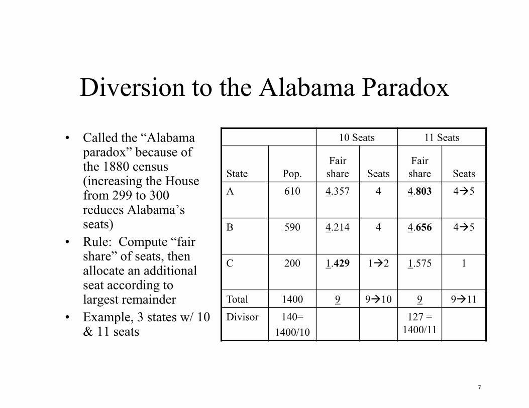
Diversion to the Alabama Paradox

• Called the “Alabama paradox” because of the 1880 census (increasing the House from 299 to 300 reduces Alabama’s seats)

• Rule: Compute “fair share” of seats, then allocate an additional seat according to largest remainder

• Example, 3 states w/ 10 & 11 seats

10 Seats 11 Seats

State Pop. Fair

share Seats Fair

share Seats

A 610 4.357 4 4.803 45

B 590 4.214 4 4.656 45

C 200 1.429 12 1.575 1

Total 1400 9 910 9 911

Divisor 140= 1400/10

127 = 1400/11

7

C B A 150

Rem

aind

er 100

50

0

0 200 400 600 800 1000 Population

Divisor = 140 Divisor = 127

8

Balinsky and Young (1982) Fair Representation

• Any method of apportionment will yield paradoxes

• No apportionment method… – Follows the quota rule

• Quota rule: If populations/seatsl = I.ddd, the state either gets I seats or I+1 seats

– Avoids the Alabama paradox – Avoids the population paradox

• Population paradox: when you have two states, and the one that grows faster loses seats to the one that grows slower

9

Method of equal proportions • “Results in a listing of the states according to a priority

value--calculated by dividing the population of each stateby the geometric mean of its current and next seats—thatassigns seats 51 through 435.”

• Practically: This method assigns seats in the House ofRepresentatives according to a ‘priority’ value. Thepriority value is determined by multiplying the populationof a state by a ‘multiplier.’ For example, following the1990 census, each of the 50 states was given one seat outof the current total of 435. The next, or 51st seat, went tothe state with the highest priority value and thus becamethat state's second seat.

Source: https://www.census.gov/topics/public-sector/congressional-apportionment.html 10

Priority values after 2010 Seat # State Priority #

51 California Seat 2 26,404,773 52 Texas Seat 2 17,867,469 53 California Seat 3 15,244,803 54 New York Seat 2 13,732,759 55 Florida Seat 2 13,364,864

. . . 431 Florida Seat 27 713,363 432 Washington Seat 10 711,867 433 Texas Seat 36 711,857 434 California Seat 53 711,308 435 Minnesota Seat 8 710,230 436 North Carolina Seat 14 709,062 437 Missouri Seat 9 708,459 438 New York Seat 28 706,336 439 New Jersey Seat 13 705,164 440 Montana Seat 2 703,158

Thanks to http://www.thegreenpapers.com/Census10/ApportionMath.phtml 11

Reapportionment Change in 2010

Courtesy of the U.S. Department of Commerce. This image is in the public domain.

12

Last seat given Next seat at 435 VA 12 (+1) 436 AL 7 (n.c.) 434 NY 34 (n.c.) 437 OR 6 (+1) 433 CA 54 (+1) 438 AZ 10 (+1) 432 TX 39 (+3) 439 MT 2 (+1) 431 CO 8 (+1) 440 MN 8 (n.c.)

… 446 RI 2 (n.c.) … 746 WY 2 (+1)

13

14

ANTICIPATED GAINS/LOSSES IN REAPPORTIONMENT2015 ESTIMATES

State numbers reflect number of congressional house seats after change put into effect.

Based on Census Bureau estimates released 12/22/2015

AZ-9 NM-3

CO-7UT-4

NV-4

OR-6

WA-10

ID-2

MT-1

WY-1

ND-1

SD-1

NE-3

MN-7

IA-4

MO-8

AR-4

LA-6

MS-4 AL-7 GA-14

TN-9

KY-6

IN-9IL-17OH-16

WI-8MI-13

NY-27MA-9

PA-17

ME-2VT-1

NH-2

RI-2CT-5

NJ-12DE-1MD-8

NC-14

SC-7

FL-28

VA-11WV-3

KS-4

OK-5

CA-53

TX-37

AK-1HI-2

CHANGE IN SEATS-1 0 +1

Image by MIT OpenCourseWare.

15

ANTICIPATED GAINS/LOSSES IN REAPPORTIONMENT2020 PROJECTIONS

State numbers reflect number of congressional house seats after change put into effect.

CHANGE IN SEATS

AZ-10 NM-3

CO-8UT-4

NV-4

OR-6

WA-10

ID-2

MT-1

WY-1

ND-1

SD-1

NE-3

MN-7

IA-4

MO-8

AR-4

LA-6

MS-4 AL-6 GA-14

TN-9

KY-6

IN-9IL-17OH-15

WI-8MI-13

NY-26MA-9

PA-17

ME-2VT-1

NH-2

RI-1CT-5

NJ-12DE-1MD-8

NC-14

SC-7

FL-29

VA-11WV-2

KS-4

OK-5

CA-53

TX-39

+1 +2 +3

AK-1HI-2

0-1

Projections to 2020 based on 2010-2015 trendline from Census Bureau estimates released 12/22/2015

Image by MIT OpenCourseWare.

Apportionment Change 2010-2030

16

-3 to -2 -4 to -3 -4 to -4-2 to -1-1 to 12 to 3 1 to 23 to 55 to 7

Image by MIT OpenCourseWare.

17

APPORTIONMENT CHANGE SINCE 1940

-15 to -10-10 to -5-5 to -11 to 5 -1 to 15 to 1010 to 30

FILLING

Image by MIT OpenCourseWare.

Recent Reapportionment Court Challenges

• Department of Commerce v. Montana, 12 S. Ct. 1415 (1992) & Franklin v. Massachusetts 112 S. Ct. 2767 (1992) – Method of equal proportions OK

• Department of Commerce v. United StatesHouse of Representatives, 525 U.S. 316 (1999) – The Census Bureau can’t sample

• Utah v. Evans, 536 U.S. 452 (2002) – “Hot deck” imputation challenged – Mormon missionaries miscounted

18

DISTRICTING

19

Districting

• Districts required in House races since Apportionment Act of 1842

• Effects of districting – Can influence overall responsiveness – Can influence quality of representation at a

micro level

20

Districting principles

• Universal principles – Compactness and contiguity – Equal population – Respect existing political communities – Political/partisan fairness

• Distinct US principle – Civil rights constraints

21

Principle 1: Compactness

• General idea: min(border/area) • Types of measures (~30 in all)

– Contorted boundary Good – Dispersion – Housing patterns

Bad 22

Three major measures

Convex Hull

Polsby-Popper

Schwartzberg

© Azavea. All rights reserved. This content is excluded from our Creative Commons license. For more information, see http://ocw.mit.edu/help/faq-fair-use/

23

Uses Polsby-Popper method (Ratio of district’s area to a circle with the same perimeter

© The Washington Post. All rights reserved. This content isexcluded from our Creative Commons license. For moreinformation, see https://ocw.mit.edu/help/faq-fair-use/.

Source: Ingraham, Christopher. "How Gerrymandered is Your Congressional District?" The Washington Post. May 15, 2014. 24

Compactness in the real world: Kansas 2011 (Good)

Courtesy of the U.S. Department of the Interior/U.S. Geological Survey. This image is in the public domain.

25

Compactness in the real world Ohio 2011 (not so good)

Courtesy of the U.S. Department of the Interior/U.S. Geological Survey. This image is in the public domain.

26

Compactness in the real world: Florida

Courtesy of the U.S. Department of the Interior/U.S. Geological Survey. This image is in the public domain.27

Florida 5th district (formerly 3rd)

© Florida Redistricting. All rights reserved. This content is excluded from our Creative Commons license. For more information, see http://ocw.mit.edu/help/faq-

fair-use/

28

Florida 20th District

© Florida Redistricting. All rights reserved. This content is excluded from our Creative Commons license. For more information, see http://ocw.mit.edu/help/faq-fair-use/

29

Old Florida Map

Courtesy of the U.S. Department of the Interior/U.S. Geological Survey. This image is in the public domain.30

New Florida Map

This content is in the public domain.

31

Principle 2: Contiguity

• General idea: keep the district together Bad Good ?

32

Contiguity in the real world: Ohio in 2010

Courtesy of the Ohio Secretary of State. Used with permission.

33

Principle 3: Equal population

• Implied by having districts • Bad: Many states before 1960s

– Illinois in 1940s (112k-914k) – Georgia in 1960s (272k-824k)

• Good: equality?

34

Equality in 2000 Ideal

District Size

Percent Overall Range

Overall Range (# of

people)

Ideal District

Size

Percent Overall Range

Overall Range (# of

people) Alabama 636,300 0.00% - Montana N/A N/A N/A Alaska N/A N/A N/A Nebraska 570,421 0.00% 0 Arizona 641,329 0.00% 0 Nevada 666,086 0.00% 6 Arkansas 668,350 0.04% 303 New Hampshire 617,893 0.10% 636 California 639,088 0.00% 1 New Jersey 647,257 0.00% 1 Colorado 614,465 0.00% 2 New Mexico 606,349 0.03% 166 Connecticut 681,113 0.00% 0 New York 654,360 0.00% 1 Delaware N/A N/A N/A North Carolina 619,178 0.00% 1 Florida 639,295 0.00% 1 North Dakota N/A N/A N/A Georgia 629,727 0.01% 72 Ohio 630,730 - -Hawaii 582,234 - - Oklahoma 690,131 - -Idaho 646,977 0.60% 3,595 Oregon 684,280 0.00% 1 Illinois 653,647 0.00% 11 Pennsylvania 646,371 0.00% 19 Indiana 675,609 0.02% 102 Rhode Island 524,160 0.00% 6 Iowa 585,265 0.02% 134 South Carolina 668,669 0.00% 2 Kansas 672,105 0.00% 33 South Dakota N/A N/A N/A Kentucky 673,628 0.00% 2 Tennessee 632,143 0.00% 5 Louisiana 638,425 0.04% 240 Texas 651,619 0.00% 1 Maine 637,462 - - Utah 744,390 0.00% 1 Maryland 662,061 0.00% 2 Vermont N/A N/A N/A Massachusetts 634,910 0.39% - Virginia 643,501 0.00% 38 Michigan 662,563 0.00% 1 Washington 654,902 0.00% 7 Minnesota 614,935 0.00% 1 West Virginia 602,781 - -Mississippi 711,165 0.00% 10 Wisconsin 670,459 0.00% 5 Missouri 621,690 0.00% 1 Wyoming N/A N/A N/A

Source: National Conf. of State Leg. 35

2012 Supreme Court Case: W.Va. Deviations Acceptable

• Tennant vs. Jefferson County Commission – Overturns “as nearly as practicable” rule

• Originally passed bill had zero population variation

• Final bill: – 1st dist: 615,991 – 2nd dist: 620,682 – 3rd dist: 616,141

36

Principle 4: Respect for existing political communities*

• Iowa• Politicians like it• May be better for

citizens• Getting more difficult

with computer draftingof districts and(nearly) equalpopulations Prepared by Iowa Legislative Services Agency for educational purposes,

this content is in the public domain.

*Upheld in Tennant v. JCC37

But, the Assembly’s another matter

Prepared by Iowa Legislative Services Agency for educational purposes, this content is in the public domain.

38

Seat

s

Principle 5: (Partisan) Fairness

• Results should be symmetrical • Results should be unbiased

Seat

s

50% Votes 50% Votes 39

Partisan Fairness

• What is the right responsiveness?

50% Votes

40

Swing ratio

• Measure of responsiveness • Concept:

– Swing ratio = ΔSeatsp/ΔVotesP

• Various ways to measure – Empirical: across time – Theoretical: “uniform swing analysis”

41

Why the swing ratio is rarely 1

Distribution of vote share

Distribution of Slope ~ 3seat share

% Dem vote

50%

50%

42

Why the swing ratio is rarely 1

Slope = 1

% Dem vote

50%

50%

43

Mayhew Diagram 2008

60

40

20

0 0% 10% 20% 30% 40% 50% 60% 70% 80% 90% 100%

Dem. vote pct.

44

Mayhew Diagram 2010

60

40

20

0 0% 10% 20% 30% 40% 50% 60% 70% 80% 90% 100%

Dem. vote pct.

45

0

20

40

60

Freq

uenc

y

0 20 40 60 80 100Dem. vote pcct.

Mayhew Diagram 2012

0

20

40

60

Freq

uenc

y

0 20 40 60 80 100 Dem. vote pcct.

46

Mayhew Diagram 2014

0

20

40

60

Freq

uenc

y

0 20 40 60 80 100 dempct

47

This image cannot currently be displayed.

Empirical swing ratio(with data from 1946-2014)

Figure 6.4

Swing ratio = 1.90:1Bias = 3.6 points

48

Cumulative distributions, 2008 & 2010

0 .2

.4

.6

.8

1

Cum

ulat

ive

dist

ribut

ion

2010

2008

0 .2 .4 .6 .8 1 Dem. pct. of vote (2-party)

49

0 .2

.4

.6

.8

1

Cum

ulat

ive

dist

ribut

ion

2010

2008

2008 swing = 1.15

2010 swing = 1.76

0 .2 .4 .6 .8 1 Dem. pct. of vote (2-party)

Cumulative distributions, 2008, 2010, & 2012

1

.8

.6

.4

2012 swing = 1.58Cum

ulat

ive

dist

ribut

ion

.2

0

0 .2 .4 .6 .8 1 Dem. pct. of vote (2-party)

50

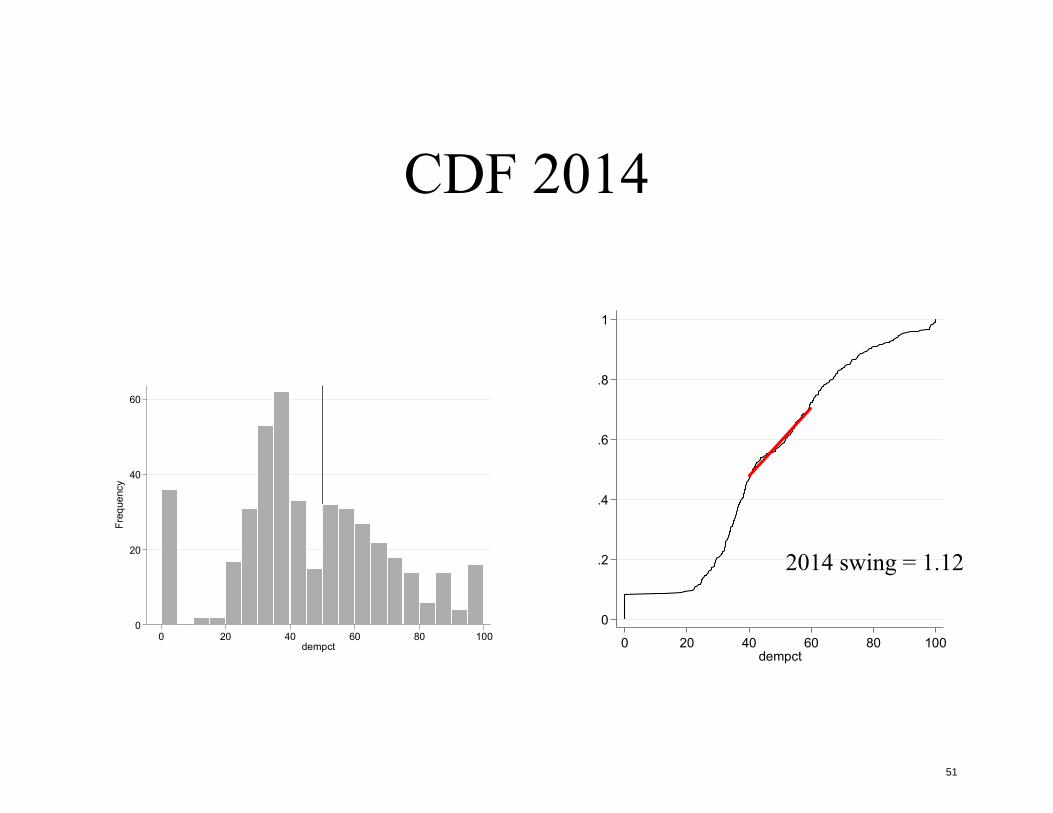
CDF 2014 Fr

eque

ncy

60

40

20

0

1

.8

.6

.4

.2

0

2014 swing = 1.12

0 20 40 60 80 100 dempct 0 20 40 60 80 100

dempct

51

Redistricting and the “Republican Advantage” in the House

• Democrats beat Republicans nationwide in popularvote in 2012, but Republicans won the Househandily – Likely to repeat in 2016

• Explanation: Republican gerrymanders in 2011 – Ohio (48% Dem vote 4D, 12R) – Florida (47% Dem vote 10D, 17R) – North Carolina (51% Dem vote 4D, 9R) – Pennsylvania (51% Dem vote 5D, 13R) – Michigan (53% Dem vote 5D, 9R) – Wisconsin (51% Dem vote 3D, 5R)

52

1

Sea

ts w

on (p

ct.)

.8

.6

.4

.2

0

NH MERI CTDEHI

MD

OR NY

CA

ILNM MN

WA AZ

IANV NJ

CO

FL WIGA MI TXWV

NC PAVA

MSUT MO OH TN IN

LA KY AL SC

KS WY AKARIDNEOK MTNDSD

MAVT

.2 .4 .6 .8 Votes won (pct.)

53

Reasons for skepticism about the “Republican gerrymander” problem

• Incumbency accounts for ~ 7 points advantage, and there are more Republican incumbents

• Democrats are more concentrated geographically than Republicans – Confirmed by Chen and Rodden)

• Florida court case will yield at most a 3-seat shift to the D’s

54

Courtesy of Jowei Chen and Johnathan Rodden. Used with permission.

Source: Jowei Chen and Jonathan Rodden, “Unintentional Gerrymandering: Political Geography and Electoral Bias in Legislatures,”

Quarterly Journal of Political Science 8(2013): 239-269. 55

Court cases concerning partisan fairness

• Davis v. Bandemer (1986) – Democrats challenge Indiana plan – Court has jurisdiction over partisan

gerrymandering – This was not a partisan gerrymander

• Vieth v. Jebelirer (2004) – Democrats challenge Pennsylvania plan – Partisan gerrymandering may be nonjusticiable – No majority to overturn Davis v. Bandemer

56

Principle 5: (Racial) fairness • From 15th amendment

– “The right of citizens of the United States to vote shall note be denied or abridged by the United States or by any State on account of race, color, or previous condition of servitude.”

• Voting Rights Act of 1965 – Prevented dilution

• Section 2: General prohibition against discrimination • Section 5: Pre-clearance for “covered” jurisdictions

– covered jurisdictions must demonstrate that a proposed voting change does not have the purpose and will not have the effect of discriminating based on race or color.

– 1980: Mobile v. Bolden • S.C. says you have to show intent

– 1982: VRA extension allows effect – 1990: Justice dept. moved to requiring maximizing minority representation through

pre-clearance – 2013: Shelby County v. Holder

• Section 4b [coverage formula] unconstitutional, thus Section 5 unenforceable • Section 2 still in force (probably) • Effect greatest in non-districting cases • Possible effects on redistricting going forward

57

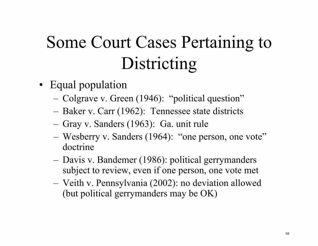
Some Court Cases Pertaining to Districting

• Equal population – Colgrave v. Green (1946): “political question” – Baker v. Carr (1962): Tennessee state districts – Gray v. Sanders (1963): Ga. unit rule – Wesberry v. Sanders (1964): “one person, one vote”

doctrine – Davis v. Bandemer (1986): political gerrymanders

subject to review, even if one person, one vote met – Veith v. Pennsylvania (2002): no deviation allowed

(but political gerrymanders may be OK)

58

VRA Cases • 1965: Dilution outlawed • 1982: Extension + Republican DOJ = Racial gerrymanders • 1993: Shaw v. Reno

– Race must be narrowly tailored to serve a compelling gov’t interest, or….

– Sandra is the law – Non-retrogression doctrine – Districting overturned in GA, NC, VA, FL, TX, LA, NY (but not IL)

• Page v. Bartels (2001): incumbency protection OK, even if it’s only minority incumbents

• Alabama Legislative Black Caucus v. Alabama (2015) (It’s a mis-reading of Section 5 to keep the % of African Americans in a district the same)

• Shelby County (2013): struck down pre-clearance formula

59

* *

*

Current Redistricting

*Plus AL&FL&NC

Courtesy of Justin Levitt. Used with permission.

Source: Justin Levitt, “All about Redistricting.” 60

Mid-Decade Redistricting Cases after 2000

• Colorado– State Supreme Court rules unconstitutional by state constitution,

SCOTUS refuses to hear• Pennsylvania

– Bandemer upheld; redistricting not overturned• Texas

– League of United Latin American Citizens et al v Perry.– Mid-decade redistricting OK– VRA problem with one state legislative district

• Virginia– Gov. McAuliffe vetoed a mid-decade state plan in 2015

61

Who Does the Redistricting?

© The Brennan Center for Justice. All rights reserved. This content is excluded from our Creative Commons license. For more information, see http://ocw.mit.edu/help/faq-fair-use/

62

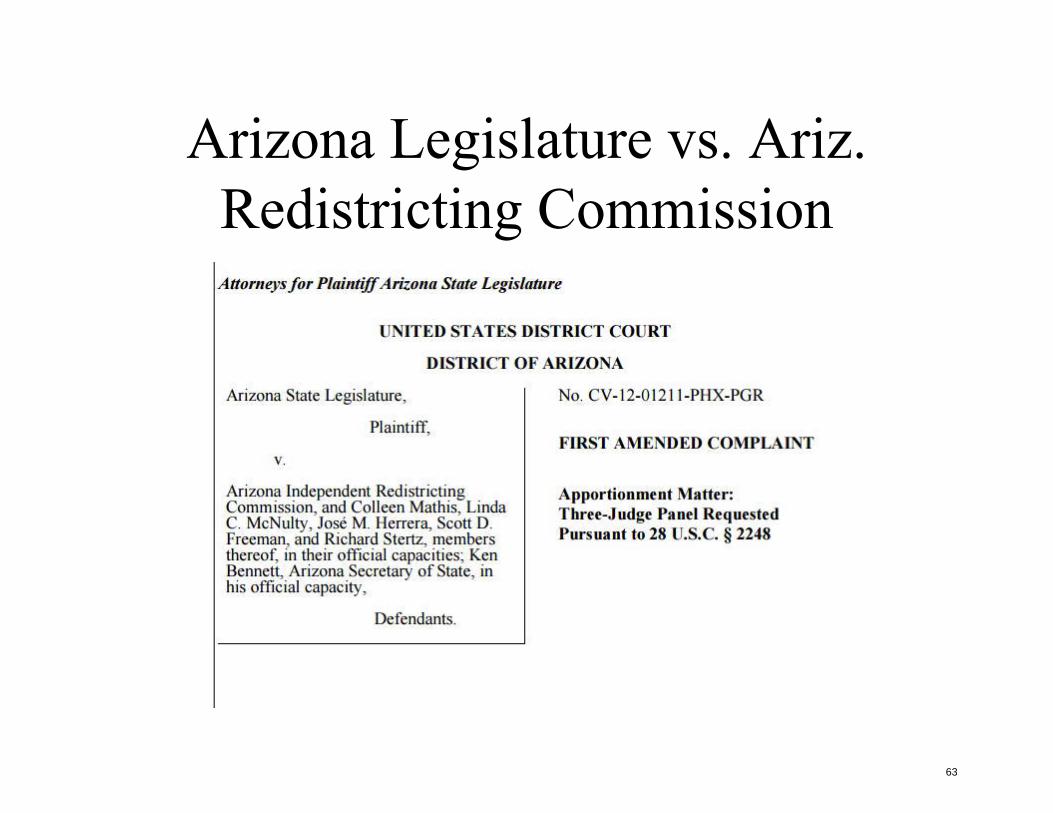
Arizona Legislature vs. Ariz. Redistricting Commission

63

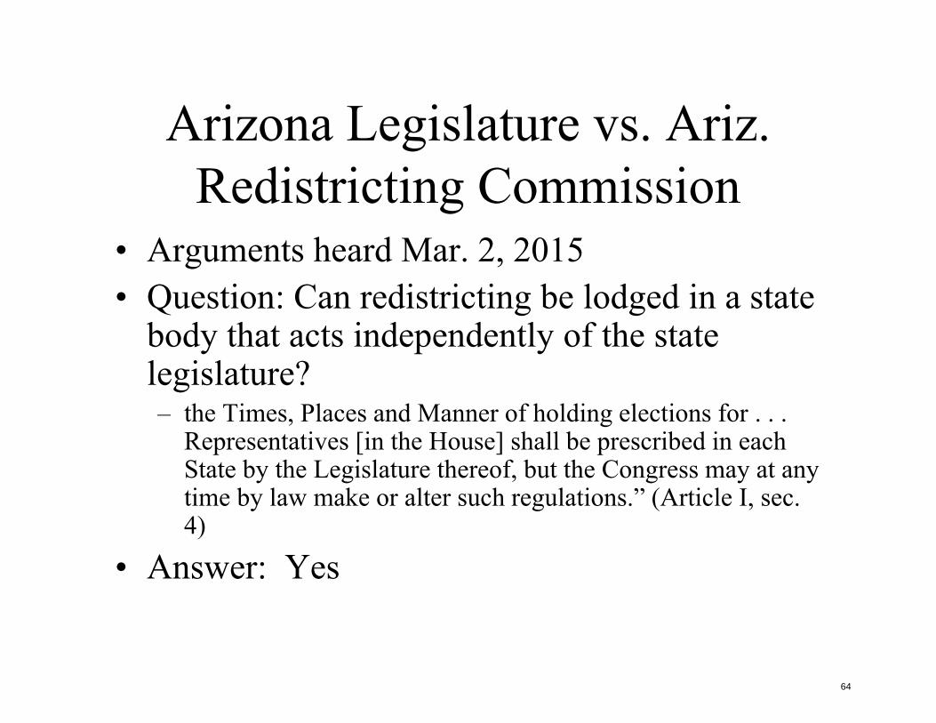
Arizona Legislature vs. Ariz. Redistricting Commission

• Arguments heard Mar. 2, 2015 • Question: Can redistricting be lodged in a state

body that acts independently of the state legislature? – the Times, Places and Manner of holding elections for . . .

Representatives [in the House] shall be prescribed in each State by the Legislature thereof, but the Congress may at any time by law make or alter such regulations.” (Article I, sec. 4)

• Answer: Yes

64

Arch & Summer Street in Boston

© Google. All rights reserved. This content is excluded from our Creative Commonslicense. For more information, see https://ocw.mit.edu/help/faq-fair-use/.

65

Arch & Summer Street in Boston Near this site stood the home of state senator Israel Thorndike, a merchant and privateer. During a visit here in 1812 by Governor Elbridge Gerry, an electoral district was oddly redrawn to provide advantage to the party in office. Shaped by political intent rather than any natural boundaries, its appearance resembled a salamander. A frustrated member of the opposition party called it a gerrymander, a term still in use today.

© Google. All rights reserved. This content is excluded from our Creative Commonslicense. For more information, see https://ocw.mit.edu/help/faq-fair-use/.

66

An aside about the states: Run-off vs. plurality rule

• The South • California’s “top-two primary”

– (really like Louisiana’s “Jungle Primary”) • Interest in “instant runoff”

67

MIT OpenCourseWarehttps://ocw.mit.edu

17.251 Congress and the American Political System IFall 2016

For information about citing these materials or our Terms of Use, visit: https://ocw.mit.edu/terms.