Embed Size (px)
Citation preview

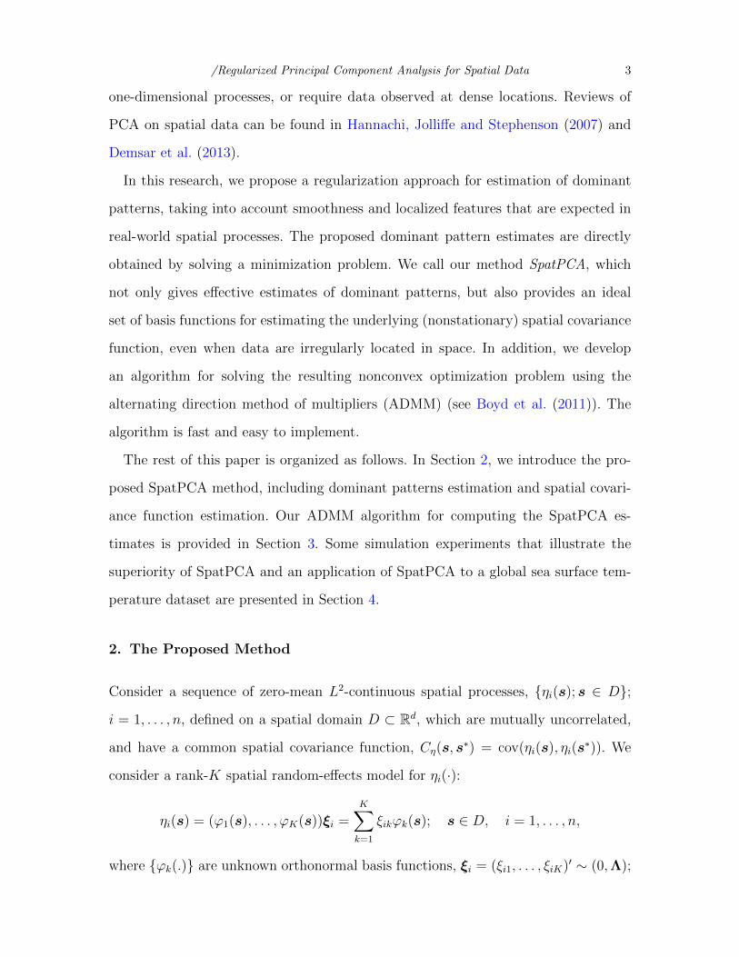
Regularized Principal ComponentAnalysis for Spatial Data
Wen-Ting WangInstitute of Statistics
National Chiao Tung [email protected]
andHsin-Cheng Huang
Institute of Statistical ScienceAcademia Sinica
Abstract: In many atmospheric and earth sciences, it is of interest to identify
dominant spatial patterns of variation based on data observed at p locations with
n repeated measurements. While principal component analysis (PCA) is com-
monly applied to find the patterns, the eigenimages produced from PCA may
be noisy or exhibit patterns that are not physically meaningful when p is large
relative to n. To obtain more precise estimates of eigenimages (eigenfunctions),
we propose a regularization approach incorporating smoothness and sparseness
of eigenfunctions, while accounting for their orthogonality. Our method allows
data taken at irregularly spaced or sparse locations. In addition, the resulting
optimization problem can be solved using the alternating direction method of
multipliers, which is computationally fast, easy to implement, and applicable
to a large spatial dataset. Furthermore, the estimated eigenfunctions provide a
natural basis for representing the underlying spatial process in a spatial random-
effects model, from which spatial covariance function estimation and spatial
prediction can be efficiently performed using a regularized fixed-rank kriging
method. Finally, the effectiveness of the proposed method is demonstrated by
several numerical examples.
Keywords: Alternating direction method of multipliers, empirical orthogonal
functions, fixed rank kriging, Lasso, non-stationary spatial covariance estima-
tion, orthogonal constraint, smoothing splines.
1
arX
iv:1
501.
0322
1v2
[st
at.M
E]
4 M
ay 2
015

/Regularized Principal Component Analysis for Spatial Data 2
1. Introduction
In many atmospheric and earth sciences, it is of interest to identify dominant spatial
patterns of variation based on data observed at p locations with n repeated measure-
ments, where p may be larger than n. The dominant patterns are the eigenimages
of the underlying (nonstationary) spatial covariance function with large eigenvalues.
A commonly used approach for estimating the eigenimages is the principal compo-
nent analysis (PCA), also known as the empirical orthogonal function analysis in
atmospheric science. However, when p is large relative to n, the leading eigenimages
produced from PCA may be noisy with high estimation variability, or exhibit some
bizarre patterns that are not physically meaningful. To enhance the interpretability,
a few approaches, such as rotation of components according to some criteria (see e.g.,
Richman (1986)), have been proposed to form more desirable patterns. However, how
to obtain a desired rotation in practice is not completely clear; see some discussion
in Hannachi, Jolliffe and Stephenson (2007).
Another approach to aid interpretation is to seek sparse or spatially localized pat-
terns, which can be done by imposing an L1 constraint or adding an L1 penalty
to an original PCA optimization formulation (Jolliffe, Uddin and Vines (2002), Zou,
Hastie and Tibshirani (2006), Shen and Huang (2008), d’Aspremont, Bach and Ghaoui
(2008), and Lu and Zhang (2012)). However, except Jolliffe, Uddin and Vines (2002)
and Lu and Zhang (2012), the PC estimates produced from these approaches may
not produce orthogonal PC loadings. Consequently, a larger number of patterns may
be needed in order to account for the total variation of the signal in a dataset.
For continuous spatial domains, the problem becomes even more challenging. In-
stead of looking for eigenimages, we need to find eigenfunctions by essentially solv-
ing an infinite dimensional problem based on data observed at possibly sparse and
irregularly spaced locations. Although some approaches have been developed using
functional principal component analysis (see e.g., Ramsay and Silverman (2005), Yao,
Muller and Wang (2005) and Huang, Shen and Buja (2008)), they typically focus on
/Regularized Principal Component Analysis for Spatial Data 3
one-dimensional processes, or require data observed at dense locations. Reviews of
PCA on spatial data can be found in Hannachi, Jolliffe and Stephenson (2007) and
Demsar et al. (2013).
In this research, we propose a regularization approach for estimation of dominant
patterns, taking into account smoothness and localized features that are expected in
real-world spatial processes. The proposed dominant pattern estimates are directly
obtained by solving a minimization problem. We call our method SpatPCA, which
not only gives effective estimates of dominant patterns, but also provides an ideal
set of basis functions for estimating the underlying (nonstationary) spatial covariance
function, even when data are irregularly located in space. In addition, we develop
an algorithm for solving the resulting nonconvex optimization problem using the
alternating direction method of multipliers (ADMM) (see Boyd et al. (2011)). The
algorithm is fast and easy to implement.
The rest of this paper is organized as follows. In Section 2, we introduce the pro-
posed SpatPCA method, including dominant patterns estimation and spatial covari-
ance function estimation. Our ADMM algorithm for computing the SpatPCA es-
timates is provided in Section 3. Some simulation experiments that illustrate the
superiority of SpatPCA and an application of SpatPCA to a global sea surface tem-
perature dataset are presented in Section 4.
2. The Proposed Method
Consider a sequence of zero-mean L2-continuous spatial processes, ηi(s); s ∈ D;
i = 1, . . . , n, defined on a spatial domain D ⊂ Rd, which are mutually uncorrelated,
and have a common spatial covariance function, Cη(s, s∗) = cov(ηi(s), ηi(s
∗)). We
consider a rank-K spatial random-effects model for ηi(·):
ηi(s) = (ϕ1(s), . . . , ϕK(s))ξi =K∑k=1
ξikϕk(s); s ∈ D, i = 1, . . . , n,
where ϕk(.) are unknown orthonormal basis functions, ξi = (ξi1, . . . , ξiK)′ ∼ (0,Λ);
/Regularized Principal Component Analysis for Spatial Data 4
i = 1, . . . , n, are uncorrelated random variables, and Λ is an unknown nonnegative-
definite matrix, denoted by Λ 0. A similar model based on given ϕk(·) was
introduced by Cressie and Johannesson (2008) and in a Bayesian framework by Kang
and Cressie (2011).
Let λkk′ be the (k, k′)-th entry of Λ. Then the spatial covariance function of ηi(·)
is:
Cη(s, s∗) = cov(ηi(s), ηi(s
∗)) =K∑k=1
K∑k′=1
λkk′ϕk(s)ϕk′(s∗). (1)
Note that Λ is not restricted to be a diagonal matrix.
Let Λ = V Λ∗V ′ be the eigen-decomposition of Λ, where V consists of K or-
thonormal vectors, and Λ∗ = diag(λ∗1, . . . , λ∗K) and λ∗1 ≥ · · · ≥ λ∗K . Let ξ∗i = V ′ξi
and
(ϕ∗1(s), . . . , ϕ∗K(s)) = (ϕ1(s), . . . , ϕK(s))V ; s ∈ D.
Then ϕ∗k are also orthonormal, and ξ∗ik ∼ (0, λ∗k); i = 1, . . . , n, k = 1, . . . , K, are
mutually uncorrelated. Therefore, we can rewrite ηi(·) in terms of ϕ∗k(·)’s:
ηi(s) = (ϕ∗1(s), . . . , ϕ∗K(s))ξ∗i =K∑k=1
ξ∗ikϕ∗k(s); s ∈ D. (2)
The above expansion is known as the Karhunen-Loeve expansion of ηi(·) (Karhunen
(1947); Loeve (1978)) with K nonzero eigenvalues, where ϕ∗k(·) is the k-th eigenfunc-
tion of Cη(·, ·) with λ∗k the corresponding eigenvalue.
Suppose that we observe data Yi = (Yi(s1), . . . , Yi(sp))′ with added white noise
εi ∼ (0, σ2I) at p spatial locations, s1, . . . , sp ∈ D, according to
Yi = ηi + εi = Φξi + εi; i = 1, . . . , n, (3)
where ηi = (ηi(s1), . . . , ηi(sp))′, Φ = (φ1, . . . ,φK) is a p×K matrix with the (j, k)-th
entry ϕk(sj), and εi’s and ξi’s are uncorrelated. Our goal is to identify the first L ≤ K
dominant patterns, ϕ1(·), . . . , ϕL(·), with relatively large λ∗1, . . . , λ∗L. Additionally, we
are interested in estimating Cη(·, ·), which is essential for spatial prediction.

/Regularized Principal Component Analysis for Spatial Data 5
Let Y = (Y1, . . . ,Yn)′ be the n×p data matrix. Throughout the paper, we assume
that the mean of Y is known as zero. So the sample covariance matrix of Y is
S = Y ′Y /n. A popular approach for estimating ϕ∗k(·) is PCA, which estimates
(ϕ∗k(s1), . . . , ϕ∗k(sp))
′ by φk, the k-th eigenvector of S, for k = 1, . . . , K. Let Φ =(φ1, . . . , φK
)be a p×K matrix formed by the first K principal component loadings.
Then Φ satisfies the following constrained optimization problem:
minΦ‖Y − Y ΦΦ′‖2F subject to Φ′Φ = IK ,
where Φ = (φ1, . . . ,φK) and ‖M‖F =(∑
i,j
m2ij
)1/2is the Frobenius norm of a
matrix M . Unfortunately, Φ tends to have high estimation variability when p is
large, n is small, or σ2 is large, due to excessive number of parameters. Consequently,
the patterns of Φ may be too noisy to be physically interpretable. In addition, for
a continuous spatial domain D, we also need to estimate ϕ∗k(s)’s for locations with
no data observed (i.e., s /∈ s1, . . . , sp), which requires applying some interpolation
and extrapolation methods; see e.g., Section 12.4 and 13.6 of Jolliffe (2002).
2.1. Regularized Spatial PCA
To prevent high estimation variability of PCA, we adopt a regularization approach
by minimizing the following objective function:
‖Y − Y ΦΦ′‖2F + τ1
K∑k=1
J(ϕk) + τ2
K∑k=1
p∑j=1
∣∣ϕk(sj)∣∣, (4)
over ϕ1(·), . . . , ϕK(·), subject to Φ′Φ = IK and φ′1Sφ1 ≥ φ′2Sφ2 ≥ · · · ≥ φ′KSφK ,
where
J(ϕ) =∑
z1+···+zd=2
∫Rd
(∂2ϕ(s)
∂xz11 . . . ∂xzdd
)2
ds,
is a roughness penalty, s = (x1, . . . , xd)′, τ1 ≥ 0 is a smoothness parameter, and τ2 ≥ 0
is a sparseness parameter. The function (4) consists of two penalty terms for control
of estimation variability. The first one is designed to enhance smoothness of ϕk(·)
/Regularized Principal Component Analysis for Spatial Data 6
through the smoothing spline penalty J(ϕk), while the second one is the L1 Lasso
penalty (Tibshirani (1996)), used to promote sparse and localized patterns. When
τ1 is larger, ϕk(·)’s tend to be smoother and vice versa. When τ2 is larger, ϕk(·)’s
are forced to become more localized, because ϕk(s)’s are forced to be zero at some
s ∈ D. On the other hand, when both τ1 and τ2 are close to zero, the estimates are
very close to those obtained from PCA. By suitably choosing τ1 and τ2, we can obtain
a good compromise among goodness of fit, smoothness of the eigenfunctions, and
sparseness of the eigenfunctions, leading to more interpretable results. Note that the
orthogonal constraint, which causes some computational difficulty, is not considered
by many PCA regularization methods (e.g., Zou, Hastie and Tibshirani (2006), Shen
and Huang (2008), Guo et al. (2010), Hong and Lian (2013)).
Although J(ϕ) involves integration, it is well known from the theory of smoothing
splines that for each k = 1, . . . , K, ϕk(·) has to be a natural cubic spline when d = 1,
and a thin-plate spline when d = 2, 3, with nodes at s1, . . . , sp. Specifically,
ϕk(s) =
p∑i=1
aig(‖s− si‖) + b0 +d∑j=1
bjxj , (5)
where s = (x1, . . . , xd)′,
g(r) =
1
16πr2 log r; if d = 2,
Γ(d/2− 2)
16πd/2r4−d; if d = 1, 3,
and the coefficients a = (a1, . . . , ap)′ and b = (b0, b1, . . . , bd)
′ satisfyG E
ET 0
ab
=
φk0
.Here G is a p×p matrix with the (i, j)-th element g(‖si−sj‖), and E is a p× (d+1)
matrix with the i-th row (1, s′i). Consequently, ϕk(·) in (5) can be expressed in terms
of φk. Additionally, the roughness penalty can also be written as
J(ϕk) = φ′kΩφk, (6)
/Regularized Principal Component Analysis for Spatial Data 7
with Ω a known p× p matrix determined only by s1, . . . , sp. The readers are referred
to Green and Silverman (1994) for more details regarding smoothing splines.
From (4) and (6), the proposed SpatPCA estimate of Φ can be written as:
Φτ1,τ2 = arg minΦ:Φ′Φ=IK
‖Y − Y ΦΦ′‖2F + τ1
K∑k=1
φ′kΩφk + τ2
K∑k=1
p∑j=1
|φjk| , (7)
subject to φ′1Sφ1 ≥ φ′2Sφ2 ≥ · · · ≥ φ′KSφK . The resulting estimates of ϕ1(·), . . . , ϕK(·)
then follow directly from (5). When no confusion may arise, we shall simply write
Φτ1,τ2 as Φ. Note that the SpatPCA estimate of (7) reduces to a sparse PCA esti-
mate of Zou, Hastie and Tibshirani (2006) if the orthogonal constraint is dropped
and Ω = I, where no spatial structure is considered.
The tuning parameters τ1 and τ2 are selected using M -fold cross-validation (CV).
First, we partition 1, . . . , n into M parts with as close to the same size as possible.
Let Y (m) be the sub-matrix of Y corresponding to the m-th part, for m = 1, . . . ,M .
For each part, we treat Y (m) as the validation data, and obtain the estimate Φ(−m)τ1,τ2
of Φ for (τ1, τ2) ∈ A based on the remaining data Y (−m) using the proposed method,
where A ⊂ [0,∞)2 is a candidate index set. The proposed CV criterion based on the
residual sum of squares is:
CV1(τ1, τ2) =1
M
M∑m=1
∥∥Y (m) − Y (m)Φ(−m)τ1,τ2
(Φ(−m)τ1,τ2
)′∥∥2F, (8)
where Y (m)Φ(−m)τ1,τ2 (Φ
(−m)τ1,τ2 )′ is the projection of Y (m) onto the column space of Φ
(−m)τ1,τ2 .
The final τ1 and τ2 values are (τ1, τ2) = arg min(τ1,τ2)∈A
CV1(τ1, τ2).
2.2. Estimation of Spatial Covariance Function
For estimation of Cη(·, ·) in (1), we also need to estimate the spatial covariance pa-
rameters, σ2 and Λ. We apply the regularized least squares method of Tzeng and
Huang (2015):
(σ2, Λ
)= arg min
(σ2,Λ):σ2≥0,Λ0
1
2
∥∥S − ΦΛΦ′ − σ2I∥∥2F
+ γ‖ΦΛΦ′‖∗, (9)

/Regularized Principal Component Analysis for Spatial Data 8
where γ ≥ 0 is a tuning parameter, and ‖M‖∗ = tr((M ′M )1/2) is the nuclear norm
of M . The first term of (9) is a goodness-of-fit term, which is based on var(Yi) =
ΦΛΦ′ + σ2I. The second term of (9) is a penalty term, penalizing the eigenvalues of
ΦΛΦ′ to avoid the eigenvalues being overestimated. By suitably choosing a tuning
parameter γ, we can control the bias, while reducing the estimation variability. This
is particularly effective when K is large.
Tzeng and Huang (2015) provides a closed-form solution for Λ, but requires an
iterative procedure for solving σ2. We are able to derive closed-form expressions for
both σ2 and Λ, which are given in the following proposition with its proof given in
the Appendix.
Proposition 1. The solutions of (9) are given by
Λ = V diag(λ∗1, . . . , λ
∗K
)V ′, (10)
σ2 =
1
p− L
(tr(S)−
L∑k=1
(dk − γ
)); if d1 > γ,
1
p(tr(S)) ; if d1 ≤ γ ,
(11)
where V diag(d1, . . . , dK)V ′ is the eigen-decomposition of Φ′SΦ with d1 ≥ · · · ≥ dK,
L = max
L : dL − γ >
1
p− L
(tr(S)−
L∑k=1
(dk − γ)
), L = 1, . . . , K
,
and λ∗k = max(dk − σ2 − γ, 0); k = 1, . . . , K.
With Λ estimated by Λ =(λkk′
)K×K in (9), the proposed estimate of Cη(s, s
∗) is
Cη(s, s∗) =
K∑k=1
K∑k′=1
λkk′ ϕk(s)ϕk′(s∗), (12)
where ϕk(s) is given in (5), and the proposed estimate of (ϕ∗1(s), . . . , ϕ∗K(s)) is
(ϕ∗1(s), . . . , ϕ∗K(s)) = (ϕ1(s), . . . , ϕK(s))V ; s ∈ D.
We consider M -fold CV to select γ, assuming that Φ is known as Φ. As in the previous
section, we partition the data into M parts, Y (1), . . . ,Y (M). For m = 1, . . . ,M , we

/Regularized Principal Component Analysis for Spatial Data 9
estimate var(Y (−m)
)by Σ(−m) = Φ(−m)Λ
(−m)γ
(Φ(−m)
)′+(σ(−m)γ
)2I based on the
remaining data Y (−m), where(σ(−m)γ
)2and Λ
(−m)γ are the estimates of σ2 and Λ
from (11) and (10) based on the data Y (−m), and Φ(−m) is the sub-matrix of Φ
corresponding to Y (−m). The proposed CV criterion is given by
CV2(γ) =1
M
M∑m=1
∥∥S(m) − ΦΛ(−m)γ Φ′ − (σ2
γ)(−m)I
∥∥2F, (13)
where S(m) is the sample covariance matrix associated with Y (m). The final γ value
is γ = arg minγ≥0
CV2(γ).
3. Computation Algorithm
Solving (7) is a challenging problem especially when both the orthogonal constraint
and the L1 penalty appear simultaneously. Consequently, many regularized PCA ap-
proaches, such as sparse PCA (Zou, Hastie and Tibshirani, 2006), do not cope with
the orthogonal constraint. We adopt the ADMM algorithm by decomposing the orig-
inal constrained optimization problem into small subproblems that can be easily and
efficiently handled through an iterative procedure. This type of algorithm was devel-
oped early in Gabay and Mercier (1976), and was systematically studied by Boyd
et al. (2011) more recently.
First, the optimization problem of (7) is transferred into the following equivalent
problem by adding an n×K parameter matrix Q:
minΦ,Q∈Rp×K
‖Y − Y ΦΦ′‖2F + τ1
K∑k=1
φ′kΩφk + τ2
K∑k=1
p∑j=1
|φjk| , (14)
subject to Q′Q = IK , φ′1Sφ1 ≥ φ′2Sφ2 ≥ · · · ≥ φ′KSφK , and a new constrain,
Φ = Q. Then the resulting constrained optimization problem of (14) is solved using
the augmented Lagrangian method with its Lagrangian given by
L(Φ,Q,Γ) = ‖Y − Y ΦΦ′‖2F + τ1
K∑k=1
φ′kΩφk + τ2
K∑k=1
p∑j=1
|φjk|
+ tr(Γ′(Φ−Q)) +ρ
2‖Φ−Q‖2F ,

/Regularized Principal Component Analysis for Spatial Data 10
subject to Q′Q = IK and φ′1Sφ1 ≥ φ′2Sφ2 ≥ · · · ≥ φ′KSφK , where Γ is a p × K
matrix of the Lagrange multipliers, and ρ > 0 is a penalty parameter to facilitate
convergence. Note that the value of ρ does not affect the original optimization prob-
lem. The ADMM algorithm iteratively updates one group of parameters at a time in
both the primal and the dual spaces until convergence. Given the initial estimates,
Q(0) and Γ(0) of Q and Γ, our ADMM algorithm consists of the following steps at
the `-th iteration:
Φ(`+1) = arg minΦ
L(Φ,Q(`),Γ(`)
)= arg min
Φ
K∑k=1
‖z(`)k −Xφk‖
2 +
p∑j=1
τ2|φjk|, (15)
Q(`+1) = arg minQ:Q′Q=IK
L(Φ(`+1),Q,Γ(`)
)= U (`)
(V (`)
)′, (16)
Γ(`+1) = Γ(`) + ρ(Φ(`+1) −Q(`+1)
), (17)
where X = (τ1Ω−Y ′Y + ρIp/2)1/2, z(`)k is the k-th column of X−1(ρQ(`) −Γ(`))/2,
U (`)D(`)(V (`)
)′is the singular value decomposition of Φ(`+1) + ρ−1Γ(`), and ρ must
be chosen large enough (e.g., twice the maximum eigenvalue of Y ′Y ) to ensure that
X is positive-definite. Note that (15) is simply a Lasso problem (Tibshirani (1996)),
which can be solved effectively using the coordinate descent algorithm (Friedman,
Hastie and Tibshirani, 2010).
Except (15), the ADMM steps given by (15)-(17) have closed-form solutions. In
fact, it is possible to develop an ADMM algorithm with complete closed-form updates
by further incorporating (15) into another ADMM step. Specifically, we can replace
φjk’s in the last term of (14) by new parameters rjk’s, and then add the constraint,
φjk = rjk for j = 1, . . . , p and k = 1, . . . , K, to form an equivalent problem:
minΦ,Q,R
‖Y − Y ΦΦ′‖2F + τ1
K∑k=1
φ′iΩφk + τ2
K∑k=1
p∑j=1
|rjk| ,
subject to Q′Q = IK , Φ = Q = R, and φ′1Sφ1 ≥ φ′2Sφ2 ≥ · · · ≥ φ′KSφK , where

/Regularized Principal Component Analysis for Spatial Data 11
rjk is the (j, k)-th element of R. Then the corresponding augmented Lagrangian is
L(Φ,Q,R,Γ1,Γ2) = ‖Y − Y ΦΦ′‖2F + τ1
K∑k=1
φ′iΩφk + τ2
K∑k=1
p∑j=1
|rjk|
+ tr(Γ′1(Φ−Q)) + tr(Γ′2(Φ−R))
+ρ
2(‖Φ−Q‖2F + ‖Φ−R‖2F ),
subject to Q′Q = IK and φ′1Sφ1 ≥ φ′2Sφ2 ≥ · · · ≥ φ′KSφK , where Γ1 and Γ2
are p ×K matrices of the Lagrange multipliers. Then the ADMM steps at the `-th
iteration are given by
Φ(`+1) = arg minΦ
L(Φ,Q(`),R(`),Γ
(`)1 ,Γ
(`)2
)=
1
2(τ1Ω + ρIp − Y ′Y )−1
ρ(Q(`) +R(`)
)− Γ1 − Γ2
, (18)
Q(`+1) = arg minQ:Q′Q=IK
L(Φ(`+1),Q,R(`),Γ
(`)1 ,Γ
(`)2
)= U (`)
(V (`)
)′, (19)
R(`+1) = arg minR
L(Φ(`+1),Q(`+1),R,Γ
(`)1 ,Γ
(`)2
)=
1
ρSτ2(ρΦ(`+1) + Γ
(`)1
), (20)
Γ(`+1)1 = Γ
(`)1 + ρ
(Φ(`+1) −Q(`+1)
), (21)
Γ(`+1)2 = Γ
(`)2 + ρ
(Φ(`+1) −R(`+1)
), (22)
whereR(0), Γ(0)1 and Γ
(0)2 are initial estimates ofR, Γ1 and Γ2, respectively,U (`)D(`)
(V (`)
)′is the singular value decomposition of Φ(`+1) + ρ−1Γ
(`)2 , and Sτ2(·) is the element-wise
soft-thresholding operator with a threshold τ2 (i.e., the (j, k)-th element of Sτ2(M )
is sign(mjk) max(|mjk − τ2|, 0), where mjk is the (j, k)-th element of M ). Similarly
to (15), ρ must be chosen large enough to ensure that τ1Ω + ρIp − Y ′Y in (18) is
positive definite.

/Regularized Principal Component Analysis for Spatial Data 12
4. Numerical Examples
In this section, we conducted some simulation experiments in one-dimensional and
two-dimensional spatial domains, and applied SpatPCA to a real-world dataset. We
compared the proposed SpatPCA with three methods: (1) PCA (τ1 = τ2 = 0); (2)
SpatPCA with the smoothness penalty only (τ2 = 0); (3) SpatPCA with the sparse-
ness penalty only (τ1 = 0), in terms of the two loss functions. The first one is a sum
of squared prediction errors:
Loss(Φ) =n∑i=1
∥∥ΦΦ′Yi −Φξi∥∥2, (23)
where Φ is the true eigenvector matrix formed by the first K eigenvectors. The second
loss function is
Loss(Cη) =
p∑i=1
p∑j=1
(Cη(si, sj)− Cη(si, sj)
)2. (24)
We applied the ADMM algorithm given by (18)-(22) to compute the SpatPCA
estimates. To facilitate convergence of ADMM, we adopted a scheme with variable ρ
based on ρ(`+1) = 1.5ρ(`) as introduced in Boyd et al. (2011), where ρ(0) is equal to
ten times the maximum eigenvalue of Y ′Y . The stopping criterion for the ADMM
algorithm is
1√p
max(‖Φ(`+1) −Φ(`)‖F , ‖Φ(`+1) −R(`+1)‖F , ‖Φ(`+1) −Q(`+1)‖F
)≤ 10−6 .
An R package to carry out SpatPCA is available upon request.
4.1. One-Dimensional Experiment
In the first experiment, we generated data according to (3) with K = 2, ξi ∼
N(0, diag(λ1, λ2)), εi ∼ N(0, I), n = 100, p = 50, s1, . . . , s50 equally spaced in
D = [−5, 5], and
φ1(s) =1
c1exp(−(x21 + · · ·+ x2d)), (25)
φ2(s) =1
c2x1 · · ·xd exp(−(x21 + · · ·+ x2d)), (26)
/Regularized Principal Component Analysis for Spatial Data 13
where s = (x1, . . . , xd)′, c1 and c2 are normalization constants such that ‖φ1‖2 =
‖φ2‖2 = 1, and d = 1. We considered three pairs of (λ1, λ2) ∈ (9, 0), (1, 0), (9, 4)
with different strengths of signals, and applied the proposed SpatPCA with three
values of K ∈ 1, 2, 5, resulting in 9 different combinations. For each combination,
we selected among 11 values of τ1 (including 0, and 10 values from 1 to 103 equally
spaced on the log scale) and 31 values of τ2 (including 0, and 30 values from 1 to 103
equally spaced on the log scale) using 5-fold CV of (8). To exploit a warm start, we
computed Φ for each τ1 along the path of τ2 from 0 to ∞, where the initial estimate
Φ(0)τ1,0
of Φ is given by the first K eigenvectors of Y ′Y − τ1Ω as its columns. Note
that Φτ1,0 is exactly equal to Φ(0)τ1,0
when Y ′Y − τ1Ω 0. We selected the tuning
parameter γ among 11 values of γ using 5-fold CV of (13), including 0, and 10 values
from 1 to d1 equally spaced on the log scale, where d1 is the largest eigenvalues of
Φ′SΦ.
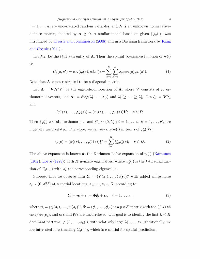
Figure 1 shows the estimates of φ1(·) and φ2(·) for the four methods based on three
different combinations of eigenvalues. Each case contains four estimated functions
based on four randomly generated datasets. As expected, the PCA estimates, which
consider no spatial structure, are very noisy, particularly when the signal-to-noise
ratio is small. By considering only the smoothness penalty with τ2 = 0, the resulting
estimates are much less noisy. But we can still see some bias, particularly around
the two ends, at which the true values are approximate zeros. On the other hand, by
considering only the sparseness penalty with τ1 = 0, the resulting estimates, while not
as noisy as those from PCA, are still noisy despite that the estimates are shrunk to
zeros at some locations. Overall, our SpatPCA estimates are very close to the targets
for all cases even when the signal-to-noise ratio is small, indicating the effectiveness
of regularization.
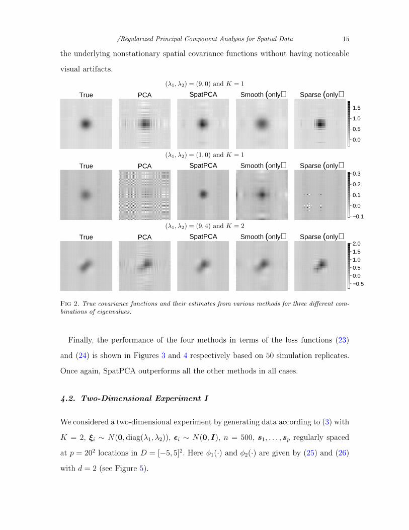
Figure 2 shows the covariance function estimates for the four methods based on
a randomly generated dataset. The proposed SpatPCA can be seen to perform con-
siderably better than the other methods for all cases by being able to reconstruct

/Regularized Principal Component Analysis for Spatial Data 14
φ1(·) based on (λ1, λ2) = (9, 0) and K = 1
−0.
20.
20.
6
PCA SpatPCA Smooth (only) Sparse (only)
φ1(·) based on (λ1, λ2) = (1, 0) and K = 1
−0.
20.
20.
6
PCA SpatPCA Smooth (only) Sparse (only)
φ1(·) based on (λ1, λ2) = (9, 4) and K = 2
−0.
20.
20.
6
PCA SpatPCA Smooth (only) Sparse (only)
φ2(·) based on (λ1, λ2) = (9, 4) and K = 2
−0.
40.
00.
4 PCA SpatPCA Smooth (only) Sparse (only)
Fig 1. Estimates of φ1(·) and φ2(·) from various methods for three different combinations of eigen-values. Each panel consists of four estimates (in four different colors) corresponding to four randomlygenerated datasets, where the dotted grey line is the true eigenfunction.
/Regularized Principal Component Analysis for Spatial Data 15
the underlying nonstationary spatial covariance functions without having noticeable
visual artifacts.
(λ1, λ2) = (9, 0) and K = 1
True PCA SpatPCA Smooth (only) Sparse (only)
0.0
0.5
1.0
1.5
(λ1, λ2) = (1, 0) and K = 1
True PCA SpatPCA Smooth (only) Sparse (only)
−0.1
0.0
0.1
0.2
0.3
(λ1, λ2) = (9, 4) and K = 2
True PCA SpatPCA Smooth (only) Sparse (only)
−0.50.00.51.01.52.0
Fig 2. True covariance functions and their estimates from various methods for three different com-binations of eigenvalues.
Finally, the performance of the four methods in terms of the loss functions (23)
and (24) is shown in Figures 3 and 4 respectively based on 50 simulation replicates.
Once again, SpatPCA outperforms all the other methods in all cases.
4.2. Two-Dimensional Experiment I
We considered a two-dimensional experiment by generating data according to (3) with
K = 2, ξi ∼ N(0, diag(λ1, λ2)), εi ∼ N(0, I), n = 500, s1, . . . , sp regularly spaced
at p = 202 locations in D = [−5, 5]2. Here φ1(·) and φ2(·) are given by (25) and (26)
with d = 2 (see Figure 5).

/Regularized Principal Component Analysis for Spatial Data 16
(λ1, λ2) = (9, 0), K = 1 (λ1, λ2) = (9, 0), K = 2 (λ1, λ2) = (9, 0), K = 5
80
120
160
200
PCA SpatPCA Smooth Sparse
200
300
400
500
PCA SpatPCA Smooth Sparse
600
800
1000
1200
PCA SpatPCA Smooth Sparse
(λ1, λ2) = (1, 0), K = 1 (λ1, λ2) = (1, 0), K = 2 (λ1, λ2) = (1, 0), K = 5
100
200
300
400
PCA SpatPCA Smooth Sparse
200
300
400
500
600
PCA SpatPCA Smooth Sparse
600
800
1000
1200
PCA SpatPCA Smooth Sparse
(λ1, λ2) = (9, 4), K = 1 (λ1, λ2) = (9, 4), K = 2 (λ1, λ2) = (9, 4), K = 5
400
500
600
PCA SpatPCA Smooth Sparse
200
250
300
350
400
PCA SpatPCA Smooth Sparse
600
800
1000
PCA SpatPCA Smooth Sparse
Fig 3. Boxplots of loss function values of (23) for various methods based on 50 simulation replicates.
(λ1, λ2) = (9, 0), K = 1 (λ1, λ2) = (9, 0), K = 2 (λ1, λ2) = (9, 0), K = 5
0
5
10
15
20
PCA SpatPCA Smooth Sparse
0
10
20
PCA SpatPCA Smooth Sparse
0
10
20
30
40
PCA SpatPCA Smooth Sparse
(λ1, λ2) = (1, 0), K = 1 (λ1, λ2) = (1, 0), K = 2 (λ1, λ2) = (1, 0), K = 5
0
1
2
3
4
5
PCA SpatPCA Smooth Sparse
0
2
4
6
8
PCA SpatPCA Smooth Sparse
0
5
10
15
PCA SpatPCA Smooth Sparse
(λ1, λ2) = (9, 4), K = 1 (λ1, λ2) = (9, 4), K = 2 (λ1, λ2) = (9, 4), K = 5
20
25
30
35
40
PCA SpatPCA Smooth Sparse
10
20
30
PCA SpatPCA Smooth Sparse
10
20
30
40
PCA SpatPCA Smooth Sparse
Fig 4. Boxplots of loss function values of (24) for various methods based on 50 simulation replicates.

/Regularized Principal Component Analysis for Spatial Data 17
φ1(·) φ2(·)
−0.4
−0.2
0.0
0.2
0.4
−0.4
−0.2
0.0
0.2
0.4
Fig 5. The true eigenimages.
As in the one-dimensional experiment, we considered three pairs of (λ1, λ2) ∈
(9, 0), (1, 0), (9, 4), and applied the proposed SpatPCA with three values of K ∈
1, 2, 5. We used 5-fold CV of (8) to select among the same 11 values of τ1 and 31
values of τ2. Similarly, we used 5-fold CV of (13) to select among the same 11 values
of γ.
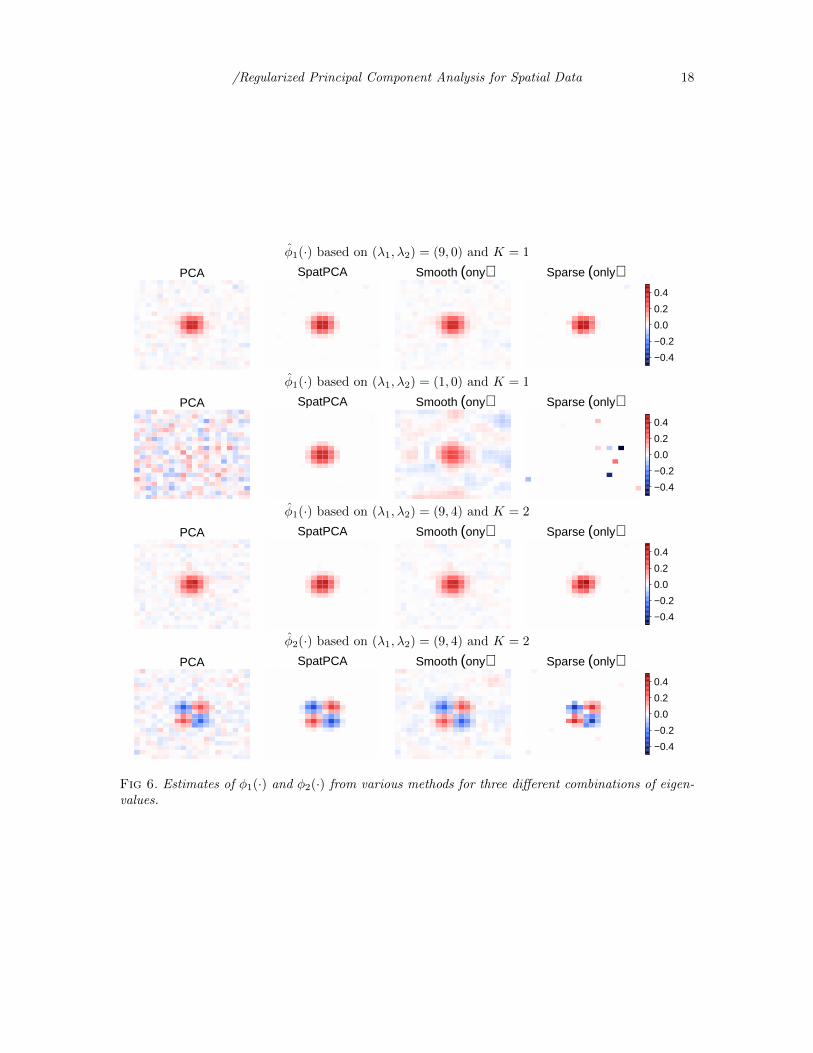
Figure 6 shows the estimates of φ1(·) and φ2(·) from the four methods for various
cases based on a randomly generated dataset. The performance of the four methods
in terms of the loss functions (23) and (24) is summarized in Figure 7 and Figure 8
respectively. Similarly to the one-dimensional examples, SpatPCA performs signifi-
cantly better than all the other methods in all cases.
4.3. An Application to a Sea Surface Temperature Dataset
Since the proposed SpatPCA works better with both smoothness and sparseness
penalties according to the simulation experiments, we applied only the proposed Spat-
PCA with both penalty terms to a sea surface temperature (SST) dataset observed in
the Indian Ocean. The data are monthly averages of SST obtained from the Met Office
Marine Data Bank (available at http://www.metoffice.gov.uk/hadobs/hadisst/)
on 1 degree latitude by 1 degree longitude (1×1) equiangular grid cells from January
2000 to December 2010 in a region between latitudes 20N and 20S and between
longitudes 39E and 120E. Out of 40 × 81 = 3, 240 grid cells, there are 420 cells
on the land where no data are available. Hence the data we used are observed at
/Regularized Principal Component Analysis for Spatial Data 18
φ1(·) based on (λ1, λ2) = (9, 0) and K = 1
PCA SpatPCA Smooth (ony) Sparse (only)
−0.4
−0.2
0.0
0.2
0.4
φ1(·) based on (λ1, λ2) = (1, 0) and K = 1
PCA SpatPCA Smooth (ony) Sparse (only)
−0.4
−0.2
0.0
0.2
0.4
φ1(·) based on (λ1, λ2) = (9, 4) and K = 2
PCA SpatPCA Smooth (ony) Sparse (only)
−0.4
−0.2
0.0
0.2
0.4
φ2(·) based on (λ1, λ2) = (9, 4) and K = 2
PCA SpatPCA Smooth (ony) Sparse (only)
−0.4
−0.2
0.0
0.2
0.4
Fig 6. Estimates of φ1(·) and φ2(·) from various methods for three different combinations of eigen-values.

/Regularized Principal Component Analysis for Spatial Data 19
(λ1, λ2) = (9, 0), K = 1 (λ1, λ2) = (9, 0), K = 2 (λ1, λ2) = (9, 0), K = 5
600
800
1000
PCA SpatPCA Smooth Sparse
1500
2000
2500
PCA SpatPCA Smooth Sparse
3000
4000
5000
6000
7000
8000
PCA SpatPCA Smooth Sparse
(λ1, λ2) = (1, 0), K = 1 (λ1, λ2) = (1, 0), K = 2 (λ1, λ2) = (1, 0), K = 5
500
1000
1500
2000
PCA SpatPCA Smooth Sparse
1000
2000
3000
4000
PCA SpatPCA Smooth Sparse
4000
6000
8000
PCA SpatPCA Smooth Sparse
(λ1, λ2) = (9, 4), K = 1 (λ1, λ2) = (9, 4), K = 2 (λ1, λ2) = (9, 4), K = 5
2500
2750
3000
3250
PCA SpatPCA Smooth Sparse
1000
1500
2000
PCA SpatPCA Smooth Sparse
3000
4000
5000
6000
7000
PCA SpatPCA Smooth Sparse
Fig 7. Boxplots of loss function values of (23) for various methods based on 50 simulation replicates.
(λ1, λ2) = (9, 0), K = 1 (λ1, λ2) = (9, 0), K = 2 (λ1, λ2) = (9, 0), K = 5
0
10
20
PCA SpatPCA Smooth Sparse
10
20
30
PCA SpatPCA Smooth Sparse
10
20
30
40
50
PCA SpatPCA Smooth Sparse
(λ1, λ2) = (1, 0), K = 1 (λ1, λ2) = (1, 0), K = 2 (λ1, λ2) = (1, 0), K = 5
0
2
4
6
8
PCA SpatPCA Smooth Sparse
0
5
10
15
PCA SpatPCA Smooth Sparse
0
10
20
30
PCA SpatPCA Smooth Sparse
(λ1, λ2) = (9, 4), K = 1 (λ1, λ2) = (9, 4), K = 2 (λ1, λ2) = (9, 4), K = 5
20
25
30
35
PCA SpatPCA Smooth Sparse
10
20
30
PCA SpatPCA Smooth Sparse
10
20
30
40
50
PCA SpatPCA Smooth Sparse
Fig 8. Boxplots of loss function values of (24) for various methods based on 50 simulation replicates.

/Regularized Principal Component Analysis for Spatial Data 20
p = 2, 780 cells and 120 time points. We first detrended the SST data by subtracting
the SST for a given cell and a given month by the average SST for that cell and that
month over the whole period. Then we randomly decomposed the data into two parts
with each part consisting of 60 time points. One part was used for training data, while
the other part was used for validation purpose.
We applied SpatPCA on the training data and chose K = 10, which appears to
be sufficiently large according to the scree plot of the sample eigenvalues (see Figure
9). We selected among 11 values of τ1 (including 0, and 10 values from 103 to 108
equally spaced on the log scale) in combination with 31 values of τ2 (including 0, and
30 values from 1 to 103 equally spaced on the log scale) using 5-fold CV of (8).
0 5 10 15 20 25 30
0.0
0.1
0.2
0.3
0.4
Component Number
Expl
aine
d va
rianc
e (%
)
Fig 9. Scree plot of sample eigenvalues based on the training data.
As shown in Figure 11 (a), the smallest CV value occurs at (τ1, τ2) = (12915, 0).
The first three patterns estimated from PCA and SpatPCA are shown in Figure 10.
Both methods identify similar patterns with the ones estimated from SpatPCA being
a bit smoother than those estimated from PCA. The first pattern is basically the
basin-wide mode and the second pattern corresponds to the east-west dipole mode
(Deser et al. (2009)).
We used the validation data to evaluate the performance between PCA and Spat-
PCA in terms of the sum of squared error (SSE), ‖Σ − Sv‖2F , where Σ is a generic
estimate of Σ based on the training data, and Sv is the sample covariance matrix
based on the validation data. For both PCA and SpatPCA, we applied 5-fold CV of

/Regularized Principal Component Analysis for Spatial Data 21
φ1(·) from PCA φ1(·) from SpatPCA
φ2(·) from PCA φ2(·) from SpatPCA
φ3(·) from PCA φ3(·) from SpatPCA
−0.04 −0.02 0.00 0.02 0.04
Fig 10. Estimated eigenimages for PCA and SpatPCA with K = 10 over a region of the IndianOcean, where the gray regions correspond to the land.
8 10 12 14 16 18
01
23
45
67
log(τ1)
log(τ
1)
−0.04
−0.02
0.00
0.02
0.04
Fig 11. Cross-validation values with respect to τ1 and τ2 on the log scale.

/Regularized Principal Component Analysis for Spatial Data 22
5 10 15 201500
1700
1900
2100
K
SSE
PCA SpatPCA
Fig 12. Sum of squared errors with respect to K for covariance matrices estimated from PCA andSpatPCA.
(13) to select among 11 values of γ, including 0, and ten values from d1/103 to d1
equally spaced on the log scale, where d1 is the largest eigenvalue of Φ′StΦ, and St is
the sample covariance matrix obtained from the training data. The SSE for PCA is
1, 607.8, which is much larger than 1, 527.0 for SpatPCA. Figure 12 shows the SSEs
with respect to various K values. The results indicate that SpatPCA is not sensitive
to the choice of K as long as K is sufficiently large. Thus, our choice of K = 10 from
the scree plot appears to be appropriate.
4.4. Two-Dimensional Experiment II
To reflect a real-world situation, we generated data by mimicking the SST dataset
analyzed in the previous subsection. Specifically, we generated data according to (3)
with K = 2, ξi ∼ N(0, diag(101.7, 17.1)), εi ∼ N(0, I), n = 60, and at the same 2, 780
locations. Here φ1(·) and φ2(·) are given by φ1(·) and φ2(·) estimated by SpatPCA in
Figure 10.
We chose K = 5 and applied the two 5-fold CVs of (8) and (13) to select the tuning
parameters (τ1, τ2) and γ respectively in the same way as in the previous subsection.
Figure 13 shows the estimates of φ1(·) and φ2(·) for PCA and SpatPCA based on a
randomly generated dataset. Because we consider a larger noise variance than those
in the previous subsection, the first two patterns estimated from PCA turn out to
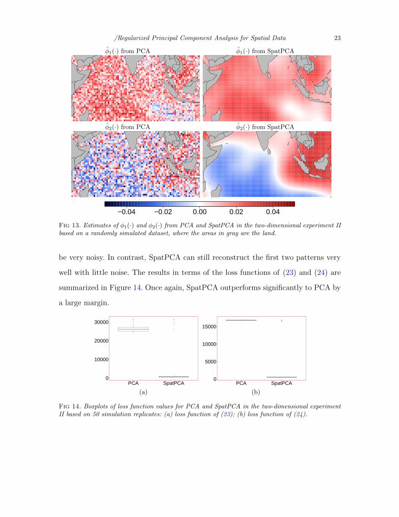
/Regularized Principal Component Analysis for Spatial Data 23
φ1(·) from PCA φ1(·) from SpatPCA
φ2(·) from PCA φ2(·) from SpatPCA
−0.04 −0.02 0.00 0.02 0.04
Fig 13. Estimates of φ1(·) and φ2(·) from PCA and SpatPCA in the two-dimensional experiment IIbased on a randomly simulated dataset, where the areas in gray are the land.
be very noisy. In contrast, SpatPCA can still reconstruct the first two patterns very
well with little noise. The results in terms of the loss functions of (23) and (24) are
summarized in Figure 14. Once again, SpatPCA outperforms significantly to PCA by
a large margin.
0
10000
20000
30000
PCA SpatPCA
0
5000
10000
15000
PCA SpatPCA
(a) (b)
Fig 14. Boxplots of loss function values for PCA and SpatPCA in the two-dimensional experimentII based on 50 simulation replicates: (a) loss function of (23); (b) loss function of (24).

/Regularized Principal Component Analysis for Spatial Data 24
Appendix
Proof of Proposition 1. First, we prove (10). From Corollary 1 of Tzeng and Huang
(2015), the minimizer of h(Λ, σ2) given σ2 is
Λ(σ2) = V diag((d1 − σ2 − γ)+, . . . , (dK − σ2 − γ)+
)V ′. (27)
Hence (10) is obtained.
Next, we prove (11). Rewrite the objective function of (9) as:
h(Λ, σ2) =1
2‖ΦΦ′SΦΦ′ − ΦΛΦ′ − σ2Ip‖2F +
1
2‖S − ΦΦ′SΦΦ′‖2F
+ σ2tr(ΦΦ′SΦΦ′ − S) + γ‖ΦΛΦ′‖∗. (28)
From (27) and (28), we have
h(Λ(σ2), σ2) =1
2‖ΦΦ′SΦΦ′ − ΦΛ(σ2)Φ′ − σ2Ip‖2F + γ‖ΦΛ(σ2)Φ′‖∗
+1
2‖S − ΦΦ′SΦΦ′‖2F + σ2tr(ΦΦ′SΦΦ′ − S)
=1
2
K∑k=1
d2k − (dk − σ2 − γ)2+
+p
2σ4 − σ2tr(S) +
1
2‖S − ΦΦ′SΦΦ′‖2F .
Minimizing h(Λ(σ2), σ2), we obtain
σ2 = arg minσ2≥0
pσ4 − 2σ2tr(S)−
K∑k=1
(dk − σ2 − γ)2+
. (29)
Clearly, if d1 ≤ γ, then σ2 =1
ptr(S). We remain to consider d1 > γ. Let
L∗ = maxL : dL − γ > σ2, L = 1, . . . , K
.
From (29), σ2 =1
p− L∗
(tr(S)−
L∗∑k=1
(dk− γ)
). It suffices to show that L∗ = L. Since
dL∗ − γ >1
p− L∗
(tr(S) −
L∗∑k=1
(dk − γ)
), by the definition of L, we have L ≥ L∗,
implying dL ≥ dL∗ . Suppose that L > L∗. It immediately follows from the definition
of L∗ that dL − γ ≤ σ2 < dL∗ − γ, which contradicts to dL ≥ dL∗ . Therefore, L = L∗.
This completes the proof.

/Regularized Principal Component Analysis for Spatial Data 25
References
Boyd, S., Parikh, N., Chu, E., Peleato, B. and Eckstein, J. (2011). Dis-
tributed optimization and statistical learning via the alternating direction method
of multipliers. Foundations and Trends in Machine Learning 3 1-124.
Cressie, N. and Johannesson, G. (2008). Fixed Rank Kriging for Very Large
Spatial Data Sets. Journal of the Royal Statistical Society. Series B 70 209-226.
d’Aspremont, A., Bach, F. and Ghaoui, L. E. (2008). Optimal solutions for
sparse principal component analysis. Journal of Machine Learning Research 9 1269-
1294.
Demsar, U., Harris, P., Brunsdon, C., Fotheringham, A. S. and
McLoone, S. (2013). Principal component analysis on spatial data: an overview.
Annals of the Association of American Geographers 103 106-128.
Deser, C., Alexander, M. A., Xie, S.-P. and Phillips, A. S. (2009). Sea sur-
face temperature variability: patterns and mechanisms. Annual Review of Marine
Science 2 115-143.
Friedman, J., Hastie, T. and Tibshirani, R. (2010). Regularization paths for
generalized linear models via coordinate descent. Journal of Statistical Software 33
1-22.
Gabay, D. and Mercier, B. (1976). A dual algorithm for the solution of nonlinear
variational problems via finite element approximation. Computer and Mathematics
with Applications 2 17-40.
Green, P. J. and Silverman, B. W. (1994). Nonparametric regression and gen-
eralized linear model: a roughness penalty approach. Chapman and Hall.
Guo, J., James., G., Levina, E., Michailidis, G. and Zhu, J. (2010). Princi-
pal component analysis with sparse fused loadings. Journal of Computational and
Graphical Statistics 19 930-946.
Hannachi, A., Jolliffe, I. T. and Stephenson, D. B. (2007). Empirical orthogo-
nal functions and related techniques in atmospheric science: A review. International

/Regularized Principal Component Analysis for Spatial Data 26
Journal of Climatology 27 1119-1152.
Hong, Z. and Lian, H. (2013). Sparse-smooth regularized singular value decompo-
sition. Journal of Multivariate Analysis 117 163-174.
Huang, J. Z., Shen, H. and Buja, A. (2008). Functional principal components
analysis via penalized rank one approximation. Electronic Journal of Statistics 2
678-695.
Jolliffe, I. T. (2002). Principal component analysis. Wiley Online Library.
Jolliffe, I. T., Uddin, M. and Vines, S. K. (2002). Simplified EOFs–three al-
ternatives to rotation. Climate Research 20 271-279.
Kang, E. L. and Cressie, N. (2011). Bayesian Inference for the Spatial Random
Effects Model. Journal of the American Statistical Association 106 972-983.
Karhunen, K. (1947). Uber lineare methoden in der Wahrscheinlichkeitsrechnung.
Annales Academiæ Scientiarum Fennicæ Series A 37 1-79.
Loeve, M. (1978). Probability theory. Springer-Verlag, New York.
Lu, Z. and Zhang, Y. (2012). An augmented Lagrangian approach for sparse prin-
cipal component analysis. Mathematical Programming 135 149–193.
Ramsay, J. O. and Silverman, B. W. (2005). Functional data analysis, 2nd ed.
New York: Springer.
Richman, M. B. (1986). Rotation of principal components. Journal of Climatology
6 293-335.
Shen, H. and Huang, J. Z. (2008). Sparse principal component analysis via regu-
larized low rank matrix approximation. Journal of Multivariate Analysis 99 1015-
1034.
Tibshirani, R. (1996). Regression shrinkage and selection via the Lasso. Journal of
the Royal Statistical Society. Series B 58 267-288.
Tzeng, S. and Huang, H.-C. (2015). Non-stationary multivariate spatial covariance
estimation via low-rank regularization. Statistical Sinica 26 151-172.
Yao, F., Muller, H.-G. and Wang, J.-L. (2005). Functional data analysis for

/Regularized Principal Component Analysis for Spatial Data 27
sparse longitudinal data. Journal of the American Statistical Association 100 577-
590.
Zou, H., Hastie, T. and Tibshirani, R. (2006). Sparse principal component anal-
ysis. Journal of Computational and Graphical Statistics 15 265-286.