Embed Size (px)
Citation preview

Regular solutions of DAE hybrid systems
and regularization techniques ∗
Peter Kunkel † Volker Mehrmann ‡
18.04.17
Abstract. The solvability and regularity of hybrid differential-algebraic systems (DAEs) isstudied, and classical stability estimates are extended to hybrid DAE systems. Different reasonsfor non-regularity are discussed and appropriate regularization techniques are presented. Thisincludes a generalization of Filippov regularization in the case of so-called chattering. The resultsare illustrated by several numerical examples.
Keywords. Differential-algebraic equation, hybrid system, switched system, index reduction,existence and uniqueness of solutions, Filippov regularization, strangeness index, chattering.
AMS(MOS) subject classification. 34K34, 34K28, 65L80, 65L05, 34K32
1 Introduction
Differential-algebraic equations (DAEs) are widely used in the modeling process of complex dy-namical systems, see, e. g., [3, 9]. In many applications the mathematical system equations switchbetween different models. One then speaks of switched or hybrid systems, see, e. g., [4, 6, 22].Classical application areas of switched systems are robot manipulators [17], mechatronics [16],mechanical systems with dry friction [10, 20], or automatic gear-boxes [15]. Other applicationsinclude electronic circuits where different device models are used for different frequency ranges,or switching elements like diodes are used, see [22], process control in chemical engineering [1],and in control systems [24, 26], where the value of a control switches between different operationmodes. See also [12, 18] for further examples. For an overview of modeling, analysis, simulationand control of hybrid systems, see, e. g., [4, 23, 24, 25].
In this paper we study the solvability of general nonlinear hybrid systems of differential-algebraicequations and extend the work of [14, 15, 24, 25]. We characterize the existence of regular solutionsand when no regular solutions exist. We also present stability estimates for general hybrid systemsof DAEs and derive regularization techniques that allow the numerical integration.
A hybrid system of DAEs on a (nontrivial) closed interval I = [t, t] ⊆ R consists of modelequations describing the different modes of the hybrid system, switching conditions describingwhen a mode loses its validity, and transition functions describing the initiation of a new mode.Hence, a hybrid system of DAEs with J modes is described as follows. The model equations aregiven by nonlinear DAEs of the form
F j(t, xj , xj) = 0, j = 1, . . . , J,
F j : I× Djx × Djx→ Rnj
,(1)
∗Supported through the Research-in-Pairs Program at Mathematisches Forschungsinstitut Oberwolfach.†Mathematisches Institut, Universitat Leipzig, Augustusplatz 10, D-04109 Leipzig, Fed. Rep. Germany,
[email protected]. Supported by Deutsche Forschungsgemeinschaft under grant no. KU964/7-1.‡Institut fur Mathematik, MA 4-5, Technische Universitat Berlin, D-10623 Berlin, Fed. Rep. Germany,
[email protected]. Supported by European Research Council through the Advanced Grant MODSIM-CONMP.
1

where Djx,Djx ⊆ Rnj
denote the open domains of definition of the variables xj and xj in thearguments of F j .
We assume each of these mode systems to be regular in the sense that they satisfy Hypothesis 4.2of [19], see Section 2 below. In particular, for each mode we have a set Ljµj describing the possibleconsistent initial conditions for this mode.
The switching conditions have the form
Sjl (t, xj) = 0, l = 1, . . . , Lj , j = 1, . . . , J,
Sjl : I× Djx → R,(2)
together with the so-called feasible regions
Fj = {(t, xj) ∈ I× Djx | Sjl (t, x
j) ≥ 0, l = 1, . . . , Lj} (3)
in which the solution is required to lie if the system is in the jth mode.The transition functions have the form
T kjl : I× Djx → Lkµk, l = 1, . . . , Lj , j = 1, . . . , J, (4)
where k = σj(l), with σj : {1, . . . , Lj} → {1, . . . , J}, is the new mode when mode j was terminateddue to a sign change in the switching function Sjl .
For our analysis we will assume that all functions are sufficiently smooth, i. e., sufficiently oftencontinuously differentiable. In particular, we assume that all occurring derivatives exist.
The paper is organized as follows. In Section 2 we recall the basics of differential-algebraicequations and in Section 3 we discuss the regularity of hybrid DAE systems. The extension ofclassical stability estimates to hybrid DAE systems is treated in Section 4. Possible non-regularbehavior and regularization techniques for hybrid DAEs, including a generalization of the Filippovregularization, are presented in Section 5 and some numerical examples are presented in Section 6.We conclude with a summary in Section 7.
2 Preliminaries
In order to introduce the concept of regularity for solutions of hybrid DAE systems, the DAEsof the single modes must be regular. To recall the regularity of general DAEs, let F describe anonlinear DAE
F (t, x, x) = 0,F : I× Dx × Dx, Dx,Dx ⊆ Rn open,
(5)
as it is given in each mode of (1). Following an idea of Campbell, see, e. g., [7], we considerso-called derivative array equations
Fµ(t, x, y) = 0, y = (x, . . . , x(µ+1)),Fµ : I× Dx × Dy → R(µ+1)n, Dx ⊆ Rn, Dy ⊆ R(µ+1)n open,
defined by stacking F and its first µ derivatives of F on top of each other, thus
Fµ =
FddtF
...
( ddt )µF
.According to [19], regularity of the DAE (5) can be guaranteed by requiring the following hypoth-esis, in which by Fµ;z we denote the Jacobian of Fµ with respect to the variable z.
2

Hypothesis 1 Consider a DAE of the form (5). There exist integers µ, a, and d such that theset
Lµ = F−1µ ({0})
associated with F is nonempty and such that for every point (t0, x0, y0) ∈ Lµ, there exists a(sufficiently small) neighborhood U in which the following properties hold:
1. We have rankFµ;y = (µ+1)n−a on Lµ∩U such that there exists a smooth matrix function Z2
of size (µ+ 1)n× a and pointwise maximal rank, satisfying ZT2 Fµ;y = 0 on Lµ ∩ U.
2. We have rankZT2 Fµ;x = a on U such that there exists a smooth matrix function T2 of sizen× d, d = n− a, and pointwise maximal rank, satisfying ZT2 Fµ;xT2 = 0 on U.
3. We have rankFxT2 = d on U such that there exists a smooth matrix function Z1 of sizen× d and pointwise maximal rank, satisfying rankZT1 FxT2 = d on U.
If a DAE system satisfies Hypothesis 1, then the smallest µ for which this is the case is calledthe strangeness index of F and systems with µ = 0 are called strangeness-free.
We will utilize Hypothesis 1 in the following form. Given a solution x∗ : I→ Rn of the derivativearray system Fµ = 0, in the sense that there exists a continuous path (t, x∗(t),P(t)) ∈ Lµ for all
t ∈ I with x∗ = P[ In 0 ]T , Hypothesis 1 guarantees the existence of (smooth) functions F1, F2
defining a so-called reduced DAE
F1(t, x, x) = 0, (d differential equations)
F2(t, x) = 0, (a algebraic equations)(6)
with x∗ being a solution of (6). Moreover, the reduced DAE satisfies Hypothesis 1 with µ = 0and, therefore, possesses solutions for sufficiently small perturbations of the initial value x∗(t0)within the set {x0 ∈ Rn | F2(t0, x0) = 0}.
A (smooth) transformation of the variable x according to
x = Q
[x1x2
], (7)
where Q : I→ Rn×n is pointwise orthogonal, then yields a decoupled DAE of the form
x1 = L(t, x1), (d differential equations)x2 = R(t, x1), (a algebraic equations)
(8)
with appropriate (smooth) functions L,R. For details, see [19].Since for given t, every (t0, x0, y0) ∈ Lµ in a neighborhood U of (t, x∗(t),P(t)) fixes a solution of
the reduced DAE, we have a flow Φt,t0 : U→ I× Rn for all t in a sufficiently small neighborhoodof t0. The flow maps (t0, x0, y0) to (t, x(t)), where x(t) is the value of the corresponding solutionat t. Note that the existence of a (global) solution on the whole of I guarantees the existence ofΦt,t0 for all t ∈ I provided U is chosen sufficiently small.
3 Regular solutions of hybrid systems of DAEs
To study the regularity of hybrid systems of DAEs, we assume that every mode in (1) is regularin the sense that F j satisfies Hypothesis 1 with some characteristic values µj , aj , dj and a setLjµj of possible consistent initial conditions, as it was introduced in Hypothesis 1. Using then thedecoupled index reduced formulation (8) for each mode,
xj1 = Lj(t, xj1), xj2 = Rj(t, xj1), j = 1, . . . , J, (9)
one obtains transformed switching conditions (2) which have the form
Sjl (t, xj1) = 0, l = 1, . . . , Lj , j = 1, . . . , J
3

after eliminating the variables x2 with the help of the algebraic equations in (9). Accordingly, thetransition functions can be transformed to
T kjl (t, xj1) = (t, xk1), l = 1, . . . , Lj , j = 1, . . . , J, k ∈ {1, . . . , J}.
Remark 2 If a switching condition is given in the more general form
Sjl (t, xj , xj) = 0,
then it should reduce to the formSjl (t, xj1, x
j2, x
j1) = 0
before the elimination of xj2. In particular, there should be no argument xj2, since the presence
of xj2 would result in the need of a further differentiation of F j . This requirement correspondsto the possibility in the ODE case to eliminate differentiated arguments with the help of thedifferential equation.
In order to define a regular solution of a hybrid system on a given fixed interval [t0, T ], we mustdefine regular solutions of the single modes (which is already obtained by requiring Hypothesis 1for each mode) as well as a regular switching behavior. Thus, we first discuss the regularity of apiece of the overall solution that corresponds to a specific mode. In the following, we call thesepieces of the solution regular arcs.
Definition 3 Consider a hybrid DAE (1) in the interval I = [t, t] and let j ∈ {0, . . . , J}. A
function x ∈ C1(I,Rnj
) is called a regular arc (of mode j) if
1. there exists z = (x,y) such that (t, z) ∈ Ljµj and (t, x(t)) = Φjt,t(t, zj) for all t ∈ I;
2. the initial value is feasible according to (t, x) ∈ Fj and there exists an εj > 0 and a neigh-borhood U of (t, z) such that
Φjt,t0(t0, z0) ∈◦F j
for all (t0, z0) ∈ U and all t ∈ (t0, t0 + εj ], where◦F j denotes the interior of the set Fj;
3. there exists l ∈ {1, . . . , Lj} such that
(a) the end point t is a regular solution of the one-dimensional problem (Sjl◦Φjt,t)(t, z) = 0
in the sense that ddt (S
j
l◦ Φjt,t)(t, z)|t=t 6= 0,
(b) strict feasibility holds according to (Sjl◦ Φjt,t)(t, z) > 0 for all t ∈ (t, t),
(c) strict feasibility holds with respect to the other switching functions up to the end point
according to (Sjl ◦ Φjt,t)(t, z) > 0 for all t ∈ (t, t] and all l ∈ {1, . . . , Lj} with l 6= l.
Remark 4 The conditions in Definition 3 can be interpreted as follows. Condition 1. just statesthat x is solution of the DAE of mode j belonging to the (consistent) initial condition given byx(t) = x. Condition 2. requires that the initial state is feasible and the corresponding solutionstays strictly feasible according to
(Sjl ◦ Φjt,t0)(t0, z0) > 0, j = 1, . . . , J
for sufficiently small perturbations of the initial condition at least for some small time intervalwhose length can be bounded away from zero. Condition 3. requires that the end point is a regularsolution of a unique switching function along the trajectory and that no other switching conditionwas satisfied before.
To simplify the notation in the following definition of a regular solution of a hybrid system, weassume that every mode contains the termination condition t− t = 0 as a switching condition.
4

Definition 5 Consider a hybrid DAE (1) in the interval I = [t, t] . Given a collection of N ∈ Nswitching points
t = (t0, t1, · · · , tN ), t = t0 < t1 < · · · < tN = t
and a collection of modes
j = (j0, j1, · · · , jN−1), ji ∈ {1, . . . , J} for i = 0, . . . , N − 1,
a finite collectionx = (xj00 , x
j11 , . . . , x
jN−1
N−1 )
of functions xji ∈ C1([ti, ti+1],Rnji) is called a regular solution of the hybrid system (1) if xji is
a regular arc of mode ji for every i = 0, . . . , N − 1, and the following condition holds:Let
z = (zj00 , zj11 , . . . , z
jN−1
N−1 )
be the corresponding initial values and let
l = (l0, l1, . . . , lN−1)
be the uniquely defined activated switching functions according to the definition of a regular arc.Then the transitions satisfy
ji+1 = σji(li)
and(ti+1, z
ji+1
i+1 ) = (Tji+1,jili
◦ Φjiti+1,ti)(ti, zjii ), i = 0, . . . , N − 2.
Remark 6 A regular solution according to Definition 5 has the following properties. Since werequire a finite switching structure given by t and j, there is a common ε = minj∈{0,...,J} ε
j > 0for all arcs of a regular solution. By assumption, the activated switching condition in mode jN−1of the last interval is given by t− t = 0 which leads to the termination of the integration processfor the hybrid system.
The notion of a regular solution is justified by the following result.
Theorem 7 Consider a hybrid system of the form (1) and let x with corresponding t and j bea regular solution of the given hybrid system. Then (1) possesses a regular solution for everyinitial condition xj0(t0) = x0 with (t0, x
j00 , y
j00 ) ∈ Lj0µj0 from a sufficiently small neighborhood of
(t0, xj00 , y
j00 ) = (t0, z
j00 ) and the final value xjN−1(tN ) depends smoothly on x0.
Proof. Since there exists a solution of the hybrid system, there is a flow Φjit,t
(t, zjii ) for all consistent
(t, zjii ) in a neighborhood of (ti, zjii ) and all t in a neighborhood of [ti, ti+1].
By assumption, the switching point ti+1 is a regular solution of
Sjili (Φjit,ti(ti, zjii )) = 0.
Hence, by the implicit function theorem, see, e. g., [21], there exists a (smooth) function Rjili with
Sjili (Φjit,t
(t, zjii )) ≡ 0 for t = Rjili (t, zjii ).
Since the sign conditions hold for all switching functions Sjll , the so obtained t remains the first
switching point that occurs for all consistent (t, zjii ) in a neighborhood of (ti, zjii ). As a conse-
quence, at t the system changes from mode ji to mode ji+1 and Φjit,t
(t, zjii ) depends smoothly on
consistent initial values (t, zjii ) in an appropriate neighborhood of (ti, zjii ). Hence,
(t, zji+1
i+1 ) = Tji+1,jili
(Φjit,t
(t, zjii )) with t = Rjili (t, zjii )
5

depends smoothly on (t, zjii ) in an appropriate neighborhood of (ti, zjii ) and is consistent for the
mode ji+1 due to the required properties of Tji+1,jili
.In this way we have shown that small changes in the initial conditions of a mode do not change
the switching that is activated and only yield small changes in the initial condition for the nextmode.
Putting all modes together, we have shown that there exists a neighborhood of (t0, zj00 ) such that
for all consistent (t0, zj00 ) from this neighborhood the corresponding initial value problem for (1)
possesses a solution with the same collection of modes and the same activated switching functionsgiven both by the sequence j. The switching points ti and initial values zjii depend smoothly on
the initial value (t0, zj00 ). In particular, the final value xjN−1(tN ) is a smooth function of the initial
value (t0, zj00 ).
Remark 8 It follows from Theorem 7 that we have
(tN , xjN−1) = Ψ(t0, z
j00 )
with a smooth function
Ψ = ΦjN−1
tN ,tN−1◦N−2©i=0
(Tji+1,jili
◦ Φjiti+1,ti),
where
ti+1 = Rjili (ti, zjii ) =
(Rjili ◦
i−1©m=0
(Tjm+1,jmlm
◦ Φjmtm+1,tm))
(t0, zj00 ).
Remark 9 If suitable spaces for a Banach space formulation of an initial value problem for hybridDAE systems are needed, as for example in the treatment of optimal control problems for hybridsystems, then it is necessary to transform the switching structure to a fixed grid. This can forexample be done via a linear transformation
θi : [ti, ti+1]→ [i, i+ 1], θi(t) =t− ti
ti+1 − ti+ k.
To summarize, we have introduced the concept of regular solutions for hybrid systems of DAEsand we have shown that such a solution stays regular in a small neighborhood with the sameswitching structure and that we obtain a flow of the system for the whole interval I under consid-eration. In the next section we derive a stability estimate for such regular solutions.
4 Stability estimates
For ordinary differential equationsx = f(t, x) (10)
there is a well-known stability estimate which states that (under suitable assumptions) the solutiondepends Lipschitz-continuously on perturbations in the initial value and in the evaluation of theright hand side of the ODE, see, e. g., [13, Theorem I.10.3].
Theorem 10 Let x ∈ C1([t0, t1],Rn) be a solution of (10) in a real interval [t0, t1] and let x ∈C1([t0, t1],Rn) satisfy
(a) ‖x(t0)− x(t0)‖ ≤ δ,(b) ‖ ˙x(t)− f(t, x(t))‖ ≤ β for all t ∈ [t0, t1],(c) ‖f(t, x(t))− f(t, x(t))‖ ≤ L‖x(t)− x(t)‖ for all t ∈ [t0, t1],
with some constant L > 0. Then
‖x(t)− x(t)‖ ≤ eL(t−t0)δ + 1L (eL(t−t0) − 1)β for all t ∈ [t0, t1].
6

In this section we derive a corresponding stability estimate for hybrid systems of DAEs, whichincludes possible perturbations in all parts of the involved computations thus generalizing Theo-rem 7.
We first consider hybrid ODEs and consider a single mode given by (10) together with a regulararc x ∈ C1([tj , tj+1],Rn). This arc is governed by a unique switching condition denoted here by
S(t, x) = 0.
In particular, we assume that f and S are defined on a compact neighborhood of
{(t, x(t)) | t ∈ [tj , tj+1]} ⊆ R× Rn
and that(a) S(tj+1, x(tj+1)) = 0, d
dtS(tj+1, x(tj+1)) 6= 0,(b) S(t, x(t)) > 0 for all t ∈ (tj , tj+1).
In this way, the terminal point tj+1 is fixed by being the first zero larger than tj of the function
u(t) = S(t, x(t)). (11)
Suppose that x ∈ C1([tj , tj+1],Rn) is a perturbed solution which satisfies
(a) ‖x(tj)− x(tj)‖ ≤ δ,(b) |tj − tj | ≤ τ,(c) ‖ ˙x(t)− f(t, x(t))‖ ≤ β for all t ∈ [tj , tj+1],(d) |S(tj+1, x(tj+1))| ≤ σ,
(12)
for sufficiently small δ, τ, β, σ > 0. Our goal is to estimate ‖x(tj+1) − x(tj+1)‖ and |tj+1 − tj+1|.Note, however, that the correct terminal point tj+1 under perturbations may not be the first zeroof the switching function, since under perturbations we cannot guarantee the feasibility of theinitial value.
For the correct choice of the terminal point, we first observe that if τ is sufficiently small, thenthe solution x can be extended to tj even if tj is not contained in [tj , tj+1]. Since f is bounded onits compact domain of definition, say by a constant M , then it holds that
‖x(tj)− x(tj)‖ = ‖x(tj + s(tj − tj))|1
0‖ = ‖∫ 1
0x(tj + s(tj − tj))(tj − tj) ds‖
≤ maxs∈[0,1] ‖f(tj + s(tj − tj), x(tj + s(tj − tj)))‖ |tj − tj | ds ≤Mτ.(13)
It follows from this inequality and (12a) that
‖x(tj)− x(tj)‖ = ‖x(tj)− x(tj)‖+ ‖x(tj)− x(tj)‖ ≤ δ +Mτ, (14)
and Theorem 10 applied to the interval [tj , tj+1] implies that
‖x(t)− x(t)‖ ≤ eL(t−tj)(δ +Mτ) + 1L (eL(t−tj) − 1)β, (15)
as long as both functions x and x are defined and satisfy
‖f(t, x(t))− f(t, x(t))‖ ≤ L‖x(t)− x(t)‖
with some constant L > 0.Having studied the influence of a perturbation in the initial state and during the integration
of the system, we now must discuss the influence of the perturbations on the accepted switchingpoint tj+1.
Since we only detect switching points by the change of sign of the switching function along thecomputed solution, it is natural to assume that both x and x are still defined in a neighborhood
7

of their final points. This then implies that there exists a sufficiently small γ > 0 such that tj+1 isthe unique zero of u defined by (11) in the interval (tj+1 − γ, tj+1 + γ). Due to (15), the function
u(t) = S(t, x(t)) (16)
will also change sign in (tj+1 − γ, tj+1 + γ) for sufficiently small δ, τ, β > 0.For sufficiently small γ > 0, then
ddtS(t, x(t)) 6= 0 for all t ∈ (tj+1 − γ, tj+1 + γ)
and the estimate
‖ ddtS(t, x(t))− ddtS(t, x(t))‖ = ‖St(t, x(t)) + Sx(t, x(t)) ˙x(t)− St(t, x(t))− Sx(t, x(t))x(t)‖
≤ ‖St(t, x(t))− St(t, x(t))‖+ ‖Sx(t, x(t))( ˙x(t)− f(t, x(t)))‖+‖Sx(t, x(t))f(t, x(t))− Sx(t, x(t))x(t)‖
≤ D(‖x(t)− x(t)‖+ β)
holds for some constant D > 0. This shows that
ddtS(t, x(t)) 6= 0 for all t ∈ (tj+1 − γ, tj+1 + γ)
for sufficiently small δ, τ, β > 0. Hence, the function u from (16) has a unique zero in the interval(tj+1 − γ, tj+1 + γ).
We now assume that tj+1 ∈ (tj+1 − γ, tj+1 + γ) and that σ > 0 is sufficiently small. Then weconsider the nonlinear system of equations
S(t, tj+1, xj+1, σ) = 0,
defined byS(t, tj+1, xj+1, σ) = S(t, x(t, tj+1, xj+1))− σ,
where x(t, tj+1, xj+1) denotes the (local) solution (10) satisfying the initial condition x(tj+1) =xj+1.
Obviously, the function S is defined in a neighborhood of (tj+1, tj+1, x(tj+1), 0) and satisfies
(a) S(t1, tj+1, x(tj+1), 0)=S(tj+1, x(tj+1, tj+1, x1(tj+1))) = S(tj+1, x(tj+1)) = 0,
(b) ∂∂t S(tj+1, tj+1, x(tj+1), 0)=St(tj+1, x(tj+1)) + Sx(tj+1, x(tj+1))x(tj+1) 6= 0.
Thus, we can apply the implicit function theorem and we obtain that locally there exists a func-tion Z which is as smooth as S and satisfies
(a) tj+1 = Z(tj+1, x(tj+1), 0),
(b) S(Z(tj+1, xj+1, σ), tj+1, xj+1, σ) = 0 for all (tj+1, xj+1, σ).
SinceS(tj+1, tj+1, x(tj+1), S(tj+1, x(tj+1)))
= S(tj+1, x(tj+1, tj+1, x(tj+1))− S(tj+1, x(tj+1)) = 0
within the validity of the implicit function theorem for sufficiently small δ, τ, β, σ > 0, we concludethat
tj+1 = Z(tj+1, x(tj+1), S(tj+1, x(tj+1))).
Hence
|tj+1 − tj+1| = |Z(tj+1, x(tj+1), S(tj+1, x(tj+1)))− Z(tj+1, x(tj+1), 0)|≤ K(‖x(tj+1)− x(tj+1)‖+ σ),
8

with some constant K > 0. Finally, in the same way as in (13), we get
‖x(tj+1)− x(tj+1)‖ ≤ ‖x(tj+1)− x(tj+1)‖+ ‖x(tj+1)− x(tj+1)‖≤ ‖x(tj+1)− x(tj+1)‖+M |tj+1 − tj+1|.
We summarize this analysis in the following stability estimate for a single mode in a switchedsystem of ODEs.
Lemma 11 Let all assumptions in the above construction for a single mode of a hybrid system ofODEs be satisfied. Then, for sufficiently small δ, τ, β, σ > 0 there exist constants κδ, κτ , κβ , κσ > 0such that
‖x(tj+1)− x(tj+1)‖+ |tj+1 − tj+1| ≤ κδδ + κττ + κββ + κσσ. (17)
Remark 12 The unique zero in (tj+1 − γ, tj+1 + γ) of u from (16), however, does not need tobe the first zero of u beyond tj . Due to the perturbations it is possible that there exists a zeroimmediately after tj , typically together with the observation that the given initial state seemsto be infeasible. If this is the case, then the implementation of the zero finder for the switchingpoints must take care to skip such an artificial switching point in order to obtain a robust solverfor hybrid systems.
To extend Lemma 11 from a single regular arc to several regular arcs, we now assume thatx = (xj00 , x
j11 , . . . , x
jN−1
N−1 ) represents a regular solution of a hybrid system of ODEs and that
x = (xj00 , xj11 , . . . , x
jN−1
N−1 ) is an approximate solution. In particular, we assume that the sameswitching structure is valid, i. e., that we have the same modes for x and x, but instead ofswitching points t = (t0, t1, · · · , tN ) for x we may have (possibly) perturbed switching pointst = (t0, t1, · · · , tN ) for x.
For the transitions, we assume that
(a) (ti+1, xji+1
i+1 (ti+1)) = T (ti+1, xjii (ti+1)),
(b) ‖(ti+1, xji+1
i+1 (ti+1))− T (ti+1, xjii (ti+1))‖ ≤ %,
i = 0, . . . , N − 2
where for simplicity we have omitted the (uniquely fixed) lower index of the transition functions.If the transition functions are Lipschitz continuous, then we obtain that
‖(ti+1, xji+1
i+1 (ti+1))− (ti+1, xji+1
i+1 (ti+1))‖= ‖(ti+1, x
ji+1
i+1 (ti+1))− T (ti+1, xjii (ti+1))‖
+ ‖T (ti+1, xjii (ti+1))− T (ti+1, x
jii (ti+1))‖
≤ %+ U‖(ti+1, xjii (ti+1))− (ti+1, x
jii (ti+1))‖
(18)
with some constant U > 0. Combining inductively the estimates (18) for every transition withthe estimate (17) for every regular arc, we obtain
‖(tN , xjN−1
N−1 (tN ))− (tN , xjN−1
N−1 (tN ))‖ ≤ κδδ + κττ + κββ + κσσ + κ%%.
for sufficiently small δ, τ, β, σ, % > 0 with suitable constants κδ, κτ , κβ , κσ, κ% > 0.Assuming that the initial and final position are not subject to perturbations, as they typically
are given as data, we are allowed to set τ = 0 and it remains to estimate the perturbation of thefinal state.
Lemma 13 Let all assumptions in the above construction for a hybrid system of ODEs be satisfied.Then for sufficiently small δ, β, σ, % > 0, there exist constants κδ, κβ , κσ, κ% > 0 such that
‖xjN−1(tN )− xjN−1(tN )‖ ≤ κδδ + κββ + κσσ + κ%%.
9

Having obtained a stability estimate for hybrid ODEs, we can easily extend these estimates toregular hybrid systems of DAEs.
For strangeness-free DAEs in the reduced formulation (8), we use (12c) and assume that
(a) ‖ ˙xj
1(t)− L(t, xj1(t))‖ ≤ β,(b) ‖xj2(t)−R(t, xj1(t))‖ ≤ η,
for all t ∈ [tj , tj+1], (19)
for every regular arc, together with all above assumptions for the (decoupled) ordinary differentialequation for xj1 including Lipschitz continuity for all involved functions.
Since the transformation Q in (7) is only used for a theoretical reformulation of the problemto state the arising perturbations as in (19), it is not subject to computational errors. Since thecomputation of the algebraic part, given here as xj2, is not to subject to a propagation of the error,we only need to transform the initial value to get the initial value of the differential part, applythe above results for hybrid systems of ODEs to the differential part, and then consider (19b) atthe end point in order to determine the final algebraic part and final solution by transformingback according to (7). Since the involved transformations (7) are linear with bounded norm andsince
‖xjN−1
2,N−1(tN )− xjN−1
2,N−1(tN )‖≤ ‖xjN−1
2,N−1(tN )−R(tN , x1,N−1(t))‖+ ‖R(tN , x1,N−1(tN ))−R(tN , x1,N−1(tN ))‖≤ η +R‖x1,N−1(tN )− x1,N−1(tN )‖
with some constant R > 0, Lipschitz continuity is maintained and we obtain the following result.
Theorem 14 Let all assumptions in the above construction for a hybrid system of DAEs be sat-isfied. Then, for sufficiently small δ, β, η, σ, %, η > 0, there exist constants κδ, κβ , κη, κσ, κ%, κη > 0such that
‖xjN−1(tN )− xjN−1(tN )‖ ≤ κδδ + κττ + κββ + κηη + κσσ + κ%%+ κηη. (20)
Remark 15 If we assume that there are no computational errors, i. e., if β = η = σ = % = η = 0,then the estimate (20) reduces to
‖xjN−1(tN )− xjN−1(tN )‖ ≤ κδδ,
for sufficiently small δ > 0, cp. Theorem 7.
In this section we have obtained stability estimates for hybrid ODEs and extended the results toregular strangeness-free hybrid DAEs. There is, however, the immediate question what happensin the case that a hybrid system of DAEs loses regularity. In this case regularization techniquesare necessary. We discuss this issue in the next section.
5 Non-regular behavior
In this section we discuss hybrid DAEs which have a lack of regularity. In view of Definition 3,such a lack of regularity can have several reasons which include at least the following cases:
1. more than one switching condition is satisfied;
2. the switching condition has a non-regular solution;
3. there is no finite collection of switching points;
4. the flow does not lead to (Sjl ◦Φjt,t)(t, zj) > 0 for t ∈ (tj , tj + ε] for all l ∈ {1, . . . , Lj}, since
(a) the flow is in at least one of the switching surfaces, i. e., we have that (Sjl ◦Φjt,t)(t, z
j) = 0
for t ∈ (tj , tj + ε] and some l ∈ {1, . . . , Lj},
10

(b) we have instantaneous further switching, i. e., we have infeasibility due to (Sjl ◦Φjt,t)(t, z
j) <
0 for t ∈ (tj , tj + ε] and some l ∈ {1, . . . , Lj}.
Since a numerical treatment of hybrid DAEs with a non-regular solution makes no sense, it isnecessary to perform a regularization by remodeling the given problem. Some of the discussed casesof non-regularity allow for ad hoc regularization techniques, but observe that these techniques maybe non-physical, since they are not based on the physical background, but they are needed for thesensible numerical integration and they may also give an indication for a possible reformulationon physical grounds.
5.1 Regularization techniques
In the following, we separately discuss various regularization techniques, but it should be notedthat these cases may occur simultaneously, so that it may be necessary to apply several of thesetogether in order to obtain a regularization.
1. Non-unique switching condition. If the end point (tj+1, xj(tj+1)) satisfies more than
one switching condition, then we can simply replace the current mode by selecting one of theactivated switching conditions and omitting the others. The particular choice may be viewed as adedicated hierarchy in the switching conditions.
2. Non-regular solution of the switching condition. If the solution of the equation forthe switching condition is non-regular, then small perturbations can lead to a different change ofmodes. A well-known example of this case is the modeling of billiard [6, 12], when a moving balljust touches another ball. For this example, we know that the overall solution depends smoothly onthe initial condition but that the condition number of the Jacobian that determines the switchingpoint may be very large, especially when there are several hits. In the general case, however, thereseems to be no good ad hoc strategy for regularizing the problem.
3. Infinite number of switching points. It may happen that an infinite number of switchingpoints occurs in the given integration interval. Since we have assumed this interval to be compact,an infinite number of switching points implies that there is at least one accumulation point inthe set of switching points. A prominent example for this case is the bouncing ball [6, 12], whenthe ball loses a certain percentage of its momentum with every bounce. A simple regularizationstrategy in this case is to characterize the behavior of the physical system after the accumulationpoint by a mode and to switch to this mode a sufficiently small amount of time before we reachthe accumulation point.
4.(a) Flow in switching surface. In the case that the flow is in the switching surface, wehave that
(Sjl ◦ Φjt,tj )(tj , zj0) = 0 for all t ∈ [tj , tj + ε]
holds for one or more l ∈ {1, . . . , Lj}. But this means nothing else than that these Sjl are firstintegrals of the DAE of mode j. Thus, we actually have an overdetermined but consistent systemof DAEs of the form
F j(t, xj , xj) = 0,
Sj(t, xj) = 0, (21)
where Sj gathers all the first integrals among the switching functions. To study the propertiesof this system, we go over to the formulation (9) so that (21) takes the form
xj1 = Lj(t, xj1),
xj2 = Rj(t, xj1),
0 = Sj(t, xj1, xj2).
11
Thus, we have additional constraints of the form
Sj(t, xj1,Rj(t, xj1)) = 0, (22)
which may in parts be trivial equations 0 = 0. Of course, these redundant equations can besimply omitted. Assuming then that d
dxj1
Sj has full row rank, we can solve (22) for some of the
components of x1. For these components, the corresponding differential equations contained inxj1 = Lj(t, xj1) are redundant and can be omitted. If we denote by Pj the projector which selects
the components of xj1 that are not fixed by (22), then we get a DAE of the form
Pj xj1 = PjLj(t, xj1),
xj2 = Rj(t, xj1),
0 = Sj(t, xj1, xj2). (23)
The original mode j then should be replaced by the regular DAE (23), together with the switchingfunctions which were not first integrals of the original DAE. Of course, the actual constructionshould and can be performed on the original (possibly higher-index) formulation of the mode. Forcorresponding details, see [19].
4.(b) Instantaneous further switching. The case of instantaneous further switching ischaracterized by the observation that
(Sjl ◦ Φjt,tj )(tj , xj(tj)) < 0 for all t ∈ (tj , tj + ε]
holds for one or more l ∈ {1, . . . , Lj}. Similar to the discussion in Case 1., we then must select one
of the activated switching conditions, say lj , in order to fix a unique new mode for the system. Ifwe denote the activated switching condition of mode k which has led to the current mode j by lk,then we can replace mode k by a new mode consisting of the same DAE and switching functions,but replacing σk(lk) = j by σk(lk) = m, where m = σj(lj), and the transition function T j,k
lkby
Tm,klk◦ Φjtj ,tj ◦ T
j,k
lk.
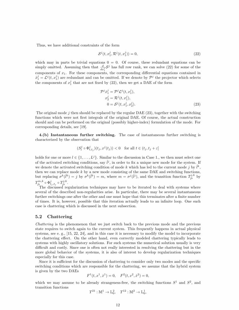
The discussed regularization techniques may have to be iterated to deal with systems whereseveral of the described non-regularities arise. In particular, there may be several instantaneousfurther switchings one after the other and one must hope that this terminates after a finite numberof times. It is, however, possible that this iteration actually leads to an infinite loop. One suchcase is chattering which is discussed in the next subsection.
5.2 Chattering
Chattering is the phenomenon that we just switch back to the previous mode and the previousstate requires to switch again to the current system. This frequently happens in actual physicalsystems, see e. g., [15, 22, 24], and in this case it is necessary to modify the model to incorporatethe chattering effect. On the other hand, even correctly modeled chattering typically leads tosystems with highly oscillatory solutions. For such systems the numerical solution usually is verydifficult and costly. Since one is often not really interested in resolving the chattering but in themore global behavior of the systems, it is also of interest to develop regularization techniquesespecially for this case.
Since it is sufficient for the discussion of chattering to consider only two modes and the specificswitching conditions which are responsible for the chattering, we assume that the hybrid systemis given by the two DAEs
F 1(t, x1, x1) = 0, F 2(t, x2, x2) = 0,
which we may assume to be already strangeness-free, the switching functions S1 and S2, andtransition functions
T 21 : M1 → L20, T 12 : M2 → L1
0,
12

x11
x21T 12
T 21
S1 = (S1)−1({0})
S2 = (S2)−1({0})
Figure 1: Occurence of chattering
where M1 = (S1)−1({0}) and M2 = (S2)−1({0}).Let T 21 : M1 →M2 and T 12 : M2 →M1 be defined by the following implications
T 21(t, x1) = (t, x2, x2) =⇒ T 21(t, x1) = (t, x2),
T 12(t, x2) = (t, x1, x1) =⇒ T 12(t, x2) = (t, x1).
Then the effect of chattering is characterized by the conditions
T 21(M1) ⊆M2, T 12(M2) ⊆M1
∂∂tS
1 + ∂∂x1S
1x1 < 0, ∂∂tS
2 + ∂∂x2S
2x2 < 0,(24)
where the sign conditions hold on the switching surfaces in L10 and L2
0 belonging to the switchingconditions that are responsible for the chattering, and by
T 21 ◦ T 12 ◦ T 21 = T 21, T 12 ◦ T 21 ◦ T 12 = T 12. (25)
This means that T 21 is an inner and outer inverse of T 12 and vice versa, [5, 8].A very simple method to regularize such a hybrid system is to introduce hysteresis [2] into the
system by moving the switching surface in such a way that the transition functions lead to theinterior of the feasible region, for example by choosing some small δ > 0, replacing the switchingconditions by
S1(t, x1) + δ = 0, S2(t, x2) + δ = 0, (26)
and taking care that the transition functions still map to M1 and M2, see the numerical experimentsbelow.
A second method to deal with chattering is the so-called Filippov regularization, see [11], in thecase that the two modes and the switching surfaces coincide. The idea of Filippov regularizationis to take the unique convex combination of the two flows which yields a flow that is restricted tothe common switching surface. Actually, this corresponds to the introduction of a new mode intothe original hybrid system together with suitable switching conditions and transfer functions.
Being originally developed for hybrid ODE models and generalized to hybrid DAEs in [15, 24, 25],we generalize this concept further to the case that the variables of the involved models do notcoincide.
For the construction, we first discuss the (autonomous) decoupled case, with d1 differential anda1 algebraic equations in the first mode and d2 differential and a2 algebraic equations in the secondmode,
(d1 eq.) x11 = L1(x11), (d2 eq.) x21 = L2(x21),(a1 eq.) x12 = R1(x11), (a2 eq.) x22 = R2(x21),
13

cp. Figure 5.2, and we assume without loss of generality that d1 ≥ d2.Chattering occurs at the time point t if
(T 21 ◦ T 12)(x21(t)) = x21(t) (27)
and the conditions
(S2 ◦ T 12)(x21(t)) = 0, S2(x21(t)) = 0,S1x11(T 12(x21(t)))L1(T 12(x21(t))) < 0, S2
x21(x21(t))L2(x21(t)) < 0 (28)
are satisfied, where the lower index as in S1x11
means the derivative with respect to x11.
A possible regularization would be to restrict the flows to the switching surface. For the secondmode this leads to
(d2 eq.) x21 = L2(x21),
(a2 eq.) x22 = R2(x21),
(1 eq.) 0 = S2(x21), (29)
which is an over-determined and inconsistent system. In particular, it is not directly evident whatwould be a meaningful flow on the manifold defined by the algebraic constraints in (29).
Observing that the differentiation of the transition relation
x21 = T 12(x11)
yieldsx21 = T 21
x11
(x11)x11 = T 21x11
(T 12(x21))L1(T 12(x21)), (30)
the idea of Filippov regularization in the ODE case is to combine the two proposed flows from (29)and (30) to a possible flow on the constraint manifold of (29).
In this way, we obtain the DAE
w11 = T 21
x11
(T 12(x21))L1(T 12(x21)),
w21 = L2(x21),
(d2 eq.) x21 = αw11 + (1− α)w2
1,(a2 eq.) x22 = R2(x21),(1 eq.) 0 = S2(x21)
(31)
for the unknowns (x21, x22, α), if we assume that the quantities w1
1, w21 are eliminated. In particular,
we only need to consider the DAE
(d2 eq.) x21 = αT 21x11
(T 12(x21))L1(T 12(x21)) + (1− α)L2(x21),
(1 eq.) 0 = S2(x21)(32)
for (x21, α).Note that (32) is a semi-explicit DAE of the form
x = f(x, y), 0 = g(x).
It is well-known that such a DAE cannot be strangeness-free, but it satisfies Hypothesis 1 withµ = 1 if gx(x)fy(x, y) is nonsingular along the solution.
To deal with this situation we assume that regularization with the help of hysteresis as describedabove is possible. In particular, we assume that extending the solution a little bit beyond theswitching surface in one mode and then switching to the other mode yields a point which isfeasible with respect to the switching condition in this mode, i. e.,
S2x21(T 21(x11(t)))T 21
x11
(x11(t))L1(x11(t)) > 0,
S1x11(T 12(x21(t)))T 12
x21
(x21(t))L2(x21(t)) > 0.(33)
14

In (32) the quantity gx(x)fy(x, y) is a scalar given by
γ = S2x21(x21)[T 21
x11
(T 12(x21))L1(T 12(x21))− L2(x21)].
Setting x11 = T 12(x21) and using (27), which gives T 21(x11) = x21, we obtain that
γ = S2x21(T 21(x11))T 21
x11
(x11)L1(x11)− S2x21(x21)L2(x21)
and this givesγ > 0 (34)
due to (28) and (33). Hence, the DAE (31) and so the DAE (32) satisfy Hypothesis 1 with µ = 1.The corresponding hidden constraint is given by
S2x21(x21)[αT 21
x11
(T 12(x21))L1(T 12(x21)) + (1− α)L2(x21)] = 0. (35)
Utilizing (34), we can solve (35) for α to obtain
α =−S2
x21(x21)L2(x21)
S2x21(x21)T 21
x11
(T 12(x21))− S2x21(x21)L2(x21)
.
Due to the sign conditions (28) and (33), we see that
α ∈ (0, 1).
Thus we actually use an appropriate convex combination of the involved flows to get a flow on theconstraint manifold of (31).
In the non-autonomous case of the form
(d1 eq.) x11 = L1(t, x11), (d2 eq.) x21 = L2(t, x21),(a1 eq.) x12 = R1(t, x11), (a2 eq.) x22 = R2(t, x21),
(36)
we must replace the relation (27) by
(T 21 ◦ T 12)(t, x21(t)) = (t, x21(t))
and, utilizingT 12(t, x21(t)) = (t, x11(t)), d
dt (T12(t, x21(t))) = (1, x11(t)),
the relations (28) by
(S2 ◦ T 12)(t, x21(t)) = 0,S1t (T 12(t, x21(t))) + S1
x11(T 12(t, x21(t)))L1(T 12(t, x21(t))) < 0,
S2(t, x21(t)) = 0,S2t (t, x21(t)) + S2
x21(t, x21(t))L2(t, x21(t)) < 0.
(37)
The relation for x21 becomes
x21 = Π22(T 21
t (T 12(t, x21)) + T 21x11
(T 12(t, x21))L1(T 12(t, x21))),
where Π22 denotes the projection onto the second argument of (t, x21). The regularized DAE then
readsw1
1 = Π22(T 21
t (T 12(t, x21)) + T 21x11
(T 12(t, x21))L1(T 12(t, x21)))),
w21 = L2(t, x21),
(d2 eq.) x21 = αw11 + (1− α)w2
1,(a2 eq.) x22 = R2(t, x21),(1 eq.) 0 = S2(t, x21).
15

Eliminating w11, w
21 yields the relevant part
(d2 eq.) x21 = αPi22(T 21t (T 12(t, x21)) + T 21
x11
(T 12(t, x21))L1(T 12(t, x21))))
+(1− α)L2(t, x21),(1 eq.) 0 = S2(t, x21).
(38)
The assumptions (33) take the form
S2t (T 21(t, x11(t))) + S2t,x2
1(T 21(t, x11(t)))T 21
x11
(t, x11(t))L1(t, x11(t)) > 0,
S1t (T 12(t, x21(t)))S1x11(T 12(t, x21(t)))T 12
x21
(t, x21(t))L2(t, x21(t)) > 0.(39)
The hidden constraint in (38) is given by
S2t (t, x21) + S2x21(t, x21)
· [αΠ22(T 21
t (T 12(t, x21)) + T 21x11
(T 12(t, x21))L1(T 12(t, x21))) + (1− α)L2(t, x21)]
= α[S2t (t, x21) + S2x21(t, x21)Π2
2(T 21t (T 12(t, x21)) + T 21
x11
(T 12(t, x21))L1(T 12(t, x21)))]
(1− α)[S2t (t, x21) + S2x21(t, x21)L2(t, x21)].
The term in the first bracket is positive due to (39), and the term in the second bracket is negativedue to (37), such that we are in the same situation as in the autonomous case leading to a well-defined α ∈ (0, 1).
In order to lift (36) to the general formulation
(d1 eq.) F 11 (t, x1, x1) = 0, (d2 eq.) F 2
1 (t, x2, x2) = 0,
(a1 eq.) F 12 (t, x1) = 0, (a2 eq.) F 2
2 (t, x2) = 0,
we consider the combined system
(d1 eq.) F 11 (t, x1, w1) = 0, (d2 eq.) F 2
1 (t, x2, w2) = 0,
[ F 12 (t, x1) = 0, ] [ F 2
2 (t, x2) = 0, ]
(a1 eq.) F 12;t(t, x
1) + F 12;x1(t, x1)w1 = 0, (a2 eq.) F 2
2;t(t, x2) + F 2
2;x2(t, x2)w2 = 0,
[ S1(t, x1) = 0, ] [ S2(t, x2) = 0, ](n1 eq.) (t, x1) = T 12(t, x3), (n2 eq.) (t, x2) = (t, x3),(n3 eq.) x3 = αΠ2
2(T 21t (T 12(t, x3)) + T 21
x1 (T 12(t, x3))w1) + (1− α)w2,
(a2 eq.) F 22 (t, x3) = 0,
(1 eq.) S2(t, x3) = 0,
(40)
where the bracketed relations are redundant and can therefore be omitted. Since the matrices[F 11,x1
F 12,x1
],
[F 21,x2
F 22,x2
]
are nonsingular due to Hypothesis 1, the first part of (40) fixes w1 ∈ Rn1
and w2 ∈ Rn2
. The
second part of (40) fixes x1 ∈ Rn1
and x2 ∈ Rn2
in terms of x3 ∈ Rn2
. The last three relations of
(40) finally form an over-determined DAE for x3 ∈ Rn2
.If we can show that the flow x3 is consistent with F 2
2 (t, x3) = 0, then there are actually onlyd2 relevant relations within the n2 equations defining x3, which would lead to a square system forthe unknowns (x3, α).
Starting from
F 22,t(t, x
3) + F 22,x2 x3(t, x3)
= F 22,t(t, x
3) + F 22,x2(t, x3)
· [αΠ22(T 21
t (T 12(t, x3)) + T 21x1 (T 12(t, x3))w1) + (1− α)w2]
= α[F 22,t(t, x
3) + F 22,x2(t, x3)Π2
2(T 21t (T 12(t, x3)) + T 21
x1 (T 12(t, x3))w1)]
+ (1− α)[F 22,t(t, x
3) + F 22,x2(t, x3)w2],
(41)
16

we see that the second bracket in the last term of (41) vanishes due to (40). Furthermore, since
F 22 (T 21(t, x1)) ≡ 0
yields
F2;t(T21(t, x1)) + F2;x2(T 21(t, x1))T 21
t (t, x1) ≡ 0,
F2;x2(T 21(t, x1))Π22T
21x1 (t, x1) ≡ 0,
the first bracket in the last term of (41) vanishes as well. Hence, the desired consistency of theabove DAE for x3 is shown.
In this section we have discussed regularization techniques for various cases of non-regularity.In particular, we have generalized the well-known Filippov regularization to the DAE case.
6 Examples and numerical experiments
To illustrate the analysis in the last sections, in this section we present some examples and numer-ical experiments. We use a C++ implementation of a DAE class for arbitrary index, see [19], usingautomatic differentiation together with a root finder, extended by an interface for mode switchingalong the lines described in the previous sections.
Example 16 A two-dimensional pendulum can be modeled via the Hamilton formalism startingwith the Hamilton function
H(p, q) = 12m−1p2 −mgL cos q,
with m the mass, L the length of the pendulum, g the gravity constant, q the generalized position(here the angle between the negative vertical axis and the pendulum), and p the correspondinggeneralized momentum. In particular, H describes the total energy consisting of kinetic andpotential energy. By the Hamilton formalism, the equations of motion are given by
p = −∇qH(p, q) = −mgL sin q,q = ∇pH(p, q) = m−1p.
It is well-known that such a system is conservative, i. e., that the total energy is preserved, due to
ddtH(p, q) = ∇pH(p, q)T p+∇qH(p, q)T q
= −∇pH(p, q)T∇qH(p, q) +∇qH(p, q)T∇pH(p, q) = 0.
Let H0 denote the total energy fixed by the initial values for p, q. Then, the switching function
S(t, p, q) = H(p, q)−H0
has the property that the flow connected with the equations of motions lies in the switching surface.Consequently, we are in Case 4.(a) of Section 5. In this example, the only algebraic constraint inthe arising overdetermined problem
p = −mgL sin q, q = m−1p, H(p, q)−H0 = 0
has the JacobianJ =
[m−1p mgL sin q
],
corresponding to ZT2 Fµ;x of Hypothesis 1. Hence, the variables not fixed by the algebraic con-straints are described by
T2 =
[−mgL sin qm−1p
],
again in the notation of Hypothesis 1. Taking T2 to project onto the relevant part of the originalequations of motion, we end up with the regularized system
−mgL sin q(p+mgL sin q) +m−1p(q −m−1p) = 0,12m−1p2 −mgL cos q −H0 = 0.
17

-0.02
-0.015
-0.01
-0.005
0
0.005
0.01
0.015
0.02
-0.2 0 0.2 0.4 0.6 0.8 1 1.2
Figure 2: Regularized chattering by generalized Filippov (black) and hysteresis (red)
Example 17 Chattering may occur in the hybrid system
x11 = −1, x12 = 0, x21 = 1− t2S11(t, x11, x
12) = x11, S2
1(t, x21) = −x21,T 211 (t, x11, x
12) = (t, x11, 1− t2), T 12
1 (t, x21) = (t, x21, 0,−1, 0)
for t ∈ (−1, 1). The generalized Filippov regularization as described in the previous section isgiven by the new mode
x12 = 0,x11 = 0,x11 = x21,S31(t, x11, x
12, x
21) = 1,
S32(t, x11, x
12, x
21) = 1− t2,
T 131 (t, x11, x
12, x
21) = (t, x11, x
12,−1, 0),
T 231 (t, x11, x
12, x
21) = (t, x21, 1− t2),
together with new switching and transfer functions
S11(t, x11, x
12) = x11, S2
1(t, x21) = −x21,T 311 (t, x11, x
12) = (t, x11, x
12, x
11, 0, 0, 0), T 32
1 (t, x21) = (t, x21, 0, x21, 0, 0, 0)
for the original modes for t ∈ (−1, 1). Figure 6 shows the solution profile of the first component ofall modes for the initial value (t0, z
10) = (−1, 1, 1,−1, 0) in Mode 1 using the generalized Filippov
regularization and hysteresis as described in (26) for δ = 0.01.
Example 18 An evaporator vessel can be modeled by the hybrid system
Ip1 = −Rpp1, Ip2 = −Rpp
2 + L2,
CL1 = −L1/Rb + fin, CL2 = −p2/I − L2/Rb + finS1(t, p1, L1) = L1 − Lth, S2(t, p2, L2) = −L2 + Lth,
T 21(t, p1, L1) = (t, p1, L1, p2, L2), T 12(t, p2, L2) = (t, p2, L2, p1, L1),
18
0.078
0.079
0.08
0.081
0.082
0.083
0.084
0 0.02 0.04 0.06 0.08 0.1 0.12 0.14
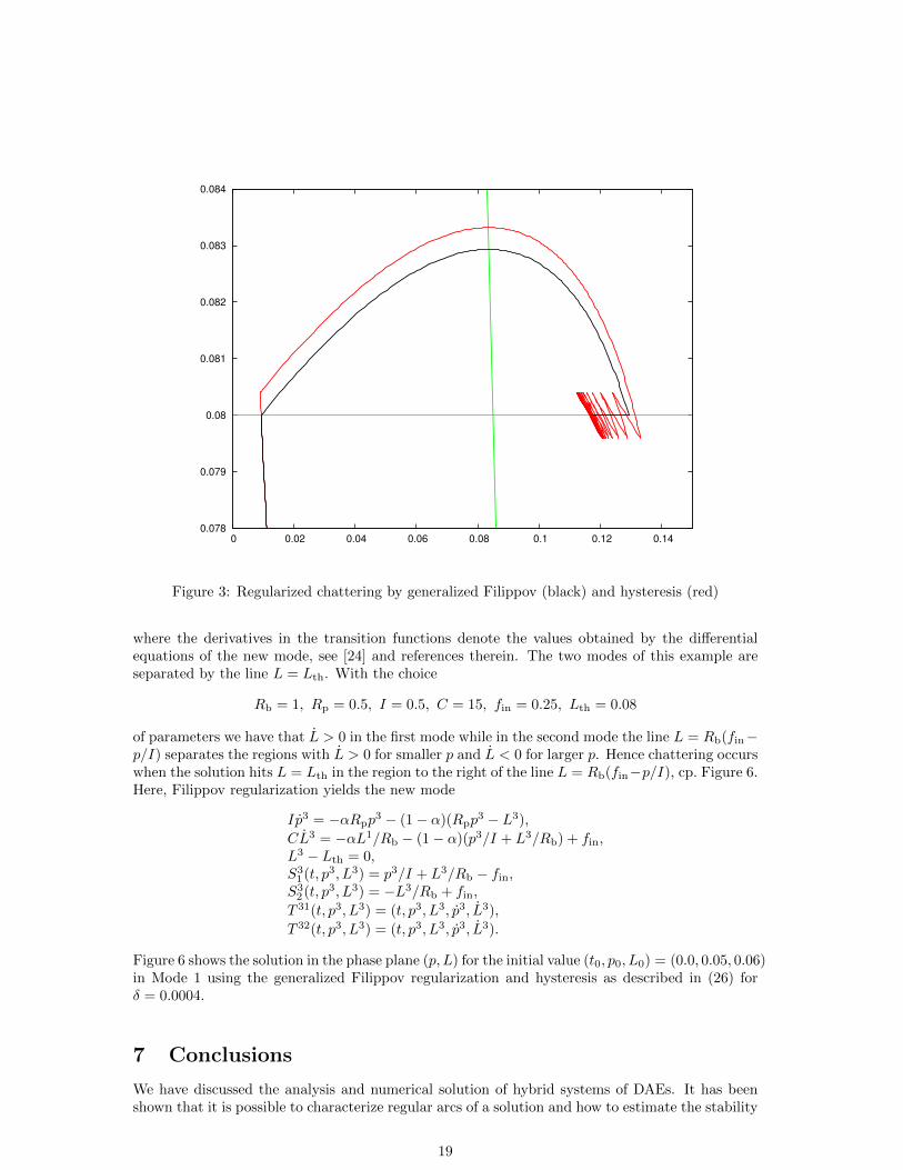
Figure 3: Regularized chattering by generalized Filippov (black) and hysteresis (red)
where the derivatives in the transition functions denote the values obtained by the differentialequations of the new mode, see [24] and references therein. The two modes of this example areseparated by the line L = Lth. With the choice
Rb = 1, Rp = 0.5, I = 0.5, C = 15, fin = 0.25, Lth = 0.08
of parameters we have that L > 0 in the first mode while in the second mode the line L = Rb(fin−p/I) separates the regions with L > 0 for smaller p and L < 0 for larger p. Hence chattering occurswhen the solution hits L = Lth in the region to the right of the line L = Rb(fin−p/I), cp. Figure 6.Here, Filippov regularization yields the new mode
Ip3 = −αRpp3 − (1− α)(Rpp
3 − L3),
CL3 = −αL1/Rb − (1− α)(p3/I + L3/Rb) + fin,L3 − Lth = 0,S31(t, p3, L3) = p3/I + L3/Rb − fin,S32(t, p3, L3) = −L3/Rb + fin,
T 31(t, p3, L3) = (t, p3, L3, p3, L3),
T 32(t, p3, L3) = (t, p3, L3, p3, L3).
Figure 6 shows the solution in the phase plane (p, L) for the initial value (t0, p0, L0) = (0.0, 0.05, 0.06)in Mode 1 using the generalized Filippov regularization and hysteresis as described in (26) forδ = 0.0004.
7 Conclusions
We have discussed the analysis and numerical solution of hybrid systems of DAEs. It has beenshown that it is possible to characterize regular arcs of a solution and how to estimate the stability
19

of a global solution. For systems which do not satisfy the regularity assumptions, we have describeddifferent regularization techniques, in particular the generalization of Filippov regularization tohybrid systems of DAEs where we even allow that the modes are formulated in different variables.We have illustrated the results via several numerical examples. It is an open problem whether thedescribed cases of non-regularity are a complete set.
References
[1] J. Agrawal, K.M. Moudgalya, and A.K. Pani. Sliding motion of discontinuous dynamicalsystems described by semi-implicit index one differential algebraic equations. Chemical Engin.Science, 61:4722–4731, 2006.
[2] J.C. Alexander and T.I. Seidman. Sliding modes in intersecting switching surfaces II: hys-teresis. Houston J. Math., 25:185–211, 1999.
[3] Modelica Association. Modelica language specification, version 3.0. Modelica Association.
[4] P.I. Barton and C.K. Lee. Modeling, simulation, sensitivity analysis, and optimization ofhybrid systems. ACM Trans. Modeling Computer Simulation, 12:256–289, 2002.
[5] A. Ben-Israel and T. N. E. Greville. Generalized Inverses: Theory and Applications. JohnWiley and Sons, New York, NY, 1973.
[6] B. Brogliato. Nonsmooth Mechanics. Springer-Verlag, New York, 1999.
[7] S. L. Campbell. A general form for solvable linear time varying singular systems of differentialequations. SIAM J. Math. Anal., 18:1101–1115, 1987.
[8] S. L. Campbell and C. D. Meyer. Generalized Inverses of Linear Transformations. Pitman,San Francisco, CA, 1979.
[9] Dynasim AB, Ideon Research Park - SE-223 70 Lund - Sweden. Dymola,Multi-EngineeringModelling and Simulation, 2006.
[10] E. Eich-Soellner and C. Fuhrer. Numerical Methods in Multibody Systems. Teubner Verlag,Stuttgart, Germany, 1998.
[11] A.F. Filippov. Differential Equations with Discontinuous Right-hand Sides. Kluwer, Dor-drecht, 1998.
[12] R. Goebel, R.G. Sanfelice, and A. Teel. Hybrid dynamical systems. Control Systems, IEEE,29:28–93, 2009.
[13] E. Hairer, S. P. Nørsett, and G. Wanner. Solving Ordinary Differential Equations I: NonstiffProblems. Springer-Verlag, Berlin, Germany, 1st edition, 1987.
[14] P. Hamann. Modellierung und Simulation von realen Planetengetrieben. Diplomarbeit, In-stitut fur Mathematik, TU Berlin, Berlin, Germany, 2003.
[15] P. Hamann and V. Mehrmann. Numerical solution of hybrid differential-algebraic equations.Comp. Meth. Appl. Mech. Eng., 197:693–705, 2008.
[16] R. Isermann. Mechatronic systems: concepts and applications. Trans. Institute of Measure-ment and Control, 22:29–55, 2000.
[17] D. Jeon and M. Tomizuka. Learning hybrid force and position control of robot manipulators.IEEE Trans. Robotic. Automat., 9:423–431, 1996.
[18] T. Krilavicius. Hybrid techniques for hybrid systems. PhD thesis, University of Twente,Enschede, 2006.
20

[19] P. Kunkel and V. Mehrmann. Differential-Algebraic Equations. Analysis and Numerical So-lution. EMS Publishing House, Zurich, Switzerland, 2006.
[20] C. Lacoursiere. Ghosts and Machines: Regularized Variational Methods for Interactive Sim-ulation of Multibodies with Dry Frictional Contacts. Phd thesis, Umea University, Sweden,2007.
[21] S. Lang. Analysis I. Addison-Wesley, Reading, MA, 3rd edition, 1973.
[22] J. Lunze and F. Lamnabhi-Laguarrigue. Handbook of Hybrid Systems Control. Theory, Toolsand Applications. Cambridge University Press, Cambridge, UK, 2009.
[23] J. Lygeros, G.J. Pappas, and S. Sastry. An Introduction to Hybrid System Modeling, Analysis,and Control. Preprints of the First Nonlinear Control Network Pedagogical School, Athens,Greece, pages 307–329, 1999.
[24] V. Mehrmann and L. Wunderlich. Hybrid systems of differential-algebraic equations – analysisand numerical solution. J. Process Control, 19:1218–1228, 2009.
[25] L. Wunderlich. Analysis and Numerical Solution of Structured and Switched Differential-Algebraic Systems. Phd thesis, TU Berlin, 2008.
[26] M. Yu, L. Wang, T. Chu, and G. Xie. Stabilization of networked control systems with datapacket dropout and network delays via switching system approach. In IEEE Conference onDecision and Control, pages 3539–3544, 2004.
21