REGULAR ARTICLES Fast Permutation Tests that …. Opdyke - JMASM Vol2 No1.pdf · REGULAR ARTICLES Fast Permutation Tests that Maximize Power Under Conventional Monte Carlo Sampling

Journal of Modern Applied Statistical Methods Copyright 2003 JMASM, Inc. May 2003, Vol. 2, No 1, 27-49 1538 � 9472/02/$30.00

27

REGULAR ARTICLES Fast Permutation Tests that Maximize Power Under Conventional Monte Carlo

Sampling for Pairwise and Multiple Comparisons

J.D. Opdyke DataMineIt

Marblehead, MA

While the distribution-free nature of permutation tests makes them the most appropriate method for hypothesis testing under a wide range of conditions, their computational demands can be runtime prohibitive, especially if samples are not very small and/or many tests must be conducted (e.g. all pairwise comparisons). This paper presents statistical code that performs continuous-data permutation tests under such conditions very quickly � often more than an order of magnitude faster than widely available commercial alternatives when many tests must be performed and some of the sample pairs contain a large sample. Also presented is an efficient method for obtaining a set of permutation samples containing no duplicates, thus maximizing the power of a pairwise permutation test under a conventional Monte Carlo approach with negligible runtime cost (well under 1% when runtimes are greatest). For multiple comparisons, the code is structured to provide an additional speed premium, making permutation-style p-value adjustments practical to use with permutation test p-values (although for relatively few comparisons at a time). �No-replacement� sampling also provides a power gain for such multiple comparisons, with similarly negligible runtime cost. Key words: Permutation test, Monte Carlo, multiple comparisons, variance reduction, multiple testing

procedures, permutation-style p-value adjustments, oversampling, no-replacement sampling

Introduction

Permutation tests are as old as modern statistics (see Fisher (1935)), and their statistical properties are well understood and thoroughly documented in the statistics literature (see Pesarin (2001) and Mielke and Berry (2001) for extensive bibliographies). Though not always as powerful as their parametric counterparts that rely on asymptotic theory, they sometimes have equal or even greater power (see Andersen and Legendre (1999) for just one example). In addition to their utility when asymptotic theory falls short (e.g. small samples and the Central Limit Theorem), permutation tests are unbiased, and when fully

J.D. Opdyke is President of DataMineIt, a statistical data mining consultancy (jdopdyke@ datamineit.com, www.datamineit.com). I owe special thanks to Geri S. Costanza, M.S., for a number of valuable insights. Any errors are my own.

enumerated, they provide gratifyingly exact results. Most important, however, is that with few exceptions, valid permutation tests rely on no distributional assumptions � only the requirement that the data satisfies the condition of exchangeability (i.e. distributional invariance under the null hypothesis to permutations of the subscripts of the data points). This gives permutation tests a very broad range of application. Until recently the major drawback of permutation tests has been their high computational demands. Even when sampling from the permutation sample space, as is typically done, rather than fully enumerating it, computer runtimes still have been prohibitive, especially if samples are not very small. Recent advances in computing speed and capacity increasingly have relaxed this constraint, but the continual development of new and computationally intensive statistical methods is easily keeping pace with such advances.

FAST PERMUTATION TESTS 28

For example, Westfall and Young (1993) convincingly demonstrated, under a broad range of real-world data conditions, the need for resampling-based multiple testing procedures. However, if the unadjusted p-values themselves are derived from resampling methods, such as permutation tests, the multiple comparisons p-value adjustment requires a computationally intensive nested loop, where a large number (thousands) of additional permutation tests must be performed for each original permutation test to properly adjust its p-value. Obviously, even if each permutation test requires just a few seconds, runtimes quickly become prohibitive if there are many p-values that need to be adjusted. Similarly, power estimation of tests based on resampling methods require the same intensive nested loop structure (see Boos and Zhang (2000) for a useful computation reduction technique), while power estimation of the multiple comparisons adjustment procedure mentioned above requires an additional (third) loop. Such examples clearly demonstrate the ongoing need to develop faster code and algorithms that are also increasingly statistically efficient, since variance reduction lessens sampling requirements which, all else equal, increases speed. The goal of the methods described below is to contribute to these efforts. Widely Available Permutation Sampling Procedures Three procedures in SAS® v8.2 � PROC NPAR1WAY, PROC MULTTEST, and PROC PLAN � and one procedure in Cytel�s Proc StatXact® v5.0 � PROC TWOSAMPL � can be used to perform two-sample nonparametric permutation tests. All but PROC PLAN sample the input dataset itself, while PROC PLAN generates a record-by-record list, each record containing a number identifying the corresponding record on the input dataset to include in the �permutation� samples. This list subsequently must be merged with the original data to obtain the corresponding data points, something PROC MULTTEST does automatically by directly generating all the �permutation� samples it uses for permutation-style p-value adjustments (these

samples, however, can be used instead as the samples for the actual permutation tests). In contrast, both PROC NPAR1WAY and PROC TWOSAMPL actually conduct the permutation test and provide a p-value, whereas the samples from both PROC MULTTEST and PROC PLAN must be manipulated �by hand� to calculate the value of the test statistic associated with the original sample pair, and then compare it to all those associated with each of the �permutation� samples to obtain a p-value. Nonetheless, effective use of PROC PLAN, as shown in benchmarks in the Results section below, is much faster than these other procedures � often more than an order of magnitude faster when one of the samples is large. The only potential problem with using PROC PLAN is that it has a sample size constraint � the product of the sum of the two sample sizes (n1 + n2) and the number of �permutation� samples being drawn (T) cannot exceed 231 (about 2.1 billion, the largest representable integer in SAS) or the procedure terminates. However, this can be circumvented by inserting calls to PROC PLAN in a loop which cycles roundup((n1 + n2)* T / 231) times, each loop drawing T * [roundup((n1 + n2)* T / 231)]-1 samples until T samples have been drawn (see code in Appendix C). This looping in and of itself does not slow execution of the procedure. All of the abovementioned procedures can perform conventional Monte Carlo sampling without replacement within a sample, as required of all but a few stylized permutation tests, but none can avoid the possibility of drawing the same sample more than once. In other words, when drawing the sample of �permutation� samples, these procedures can only draw from the sample space of samples (conditional on the data) with replacement (WR). This problem of drawing duplicate samples, its effect on the statistical power of the permutation test, and a proposed solution that maximizes power under conventional Monte Carlo sampling for both pairwise and multiple comparisons are discussed in the Methodology section below. First, the background issues of determining the number of �permutation� samples to draw, and sampling approaches other than conventional Monte Carlo, are addressed

29 J.D. OPDYKE

below. Determining the Number of Permutation Samples When drawing samples from the permutation sample space, one must determine how many samples should be drawn. Obtaining an exact p-value from a permutation test via full enumeration � i.e. by generating all possible sample combinations by reshuffling the data points of the samples at hand � quickly becomes infeasible as sample sizes increase. As shown in (1), the number of possible sample combinations becomes very large even for relatively small sample sizes (two samples of 29 observations each, for example, have 30,067,266,499,541,000 possible sample combinations).

(1) # of two-sample combinations where sample one�s size, sample two�s size, and Network algorithms (see Mehta and Patel (1983)) expand the sample size range over which exact p-values realistically may be obtained, but the rapid combinatorial expansion of the �permutation� sample space � defined as conditional on the data in (1) � still limits the full enumeration of continuous data samples to relatively small sample sizes. Sampling from the permutation sample space, however, can provide an estimate of the exact p-value via a conventional Monte Carlo approach, whereby the probability of drawing any particular sample is equal to one divided by the number of possible sample combinations, as in (2) below:

(2) (Note that permutations of the same sample do not affect this probability.) A (one-sided) permutation test p-value is simply the number of test statistic values, each corresponding to a �permutation� sample, at least as large as that based on the observed data samples; therefore, the estimated p-value based on conventional Monte Carlo sampling is simply an estimated proportion

distributed binomially. The normal approximation to the binomial distribution allows one easily to obtain specified levels of precision for this estimate, based either on the standard error (se) or the coefficient of variation (cv), as a function of T = the number of samples drawn. This is done by straightforward solutions of (3) and (4) respectively (see Brown et al. (2001) for descriptions of the �Agresti-Coull� and �Wilson� intervals � superior, if slightly more complex, alternatives to the commonly used Wald approximation shown in (3)).

(3)

(4) and for , . For example, if cv<0.10 is needed, one would solve for T in (4) using the most relevant p-value (p-value = α) and adding one to the solution so that the inequality holds (see Efron and Tibshirani, 1993, pp. 208-211 for an identical calculation). If α = 0.05, then T=1,901, which also yields an approximate 95% confidence interval, based on (3), of just under 0.01 on either side of p-value = α = 0.05. While this may be sufficiently precise for many applications, increased precision is obtainable with larger T, though as shown in Graph 1, marginal gains in precision decrease rapidly in T. (Note that the normal approximation to the binomial distribution easily satisfies the strictest criteria in the statistical literature for T = 1,901 and p-value = 0.05 (see Cochran (1977), p. 58, and Evans, et al. (1993), p. 39)).

( )1

1Prn n

S sC

= =

1n = 2n =

1 2n n n= +

( )1

1 2

1 2

!

! !n nn n

Cn n

+= =

secv

p value=

−

( )0.05 1 0.05

0.10 1,9000.05

Tcv T

−

= = ⇒ =

0.10cv < 1,901T =

( )( )1, and

p value p valuese

T

− − −≈

( )95% 1.96ci p value se≈ − ± ×


Graph 1: Permutation p-value -- cv and 1.96*se by T (# permutation samples) for p-value = alpha = 0.05

0.00

0.05

0.10

0.15

0.20

0.25

0.30

0.35

0.40

0.45

0.50

020

040

060

080

01,0

001,2

001,4

001,6

001,8

002,0

002,2

002,4

002,6

002,8

003,0

003,2

003,4

00

T

cv

0.000

0.005

0.010

0.015

0.020

0.025

0.030

0.035

0.040

0.045

1.96

*se

se*1.96 cv An efficient alternative to a fixed level of precision, however, especially when conducting many permutation tests, is increasing T only when the confidence interval of a specific test includes the critical value. Selectively tightening the confidence interval in this way avoids wasteful sampling when p-values are nowhere near the critical value of the test. Other Sampling Methods The level of precision a method provides for a given number of samples is its efficiency. The efficiency, as well as speed, of conventional Monte Carlo sampling as described above typically are inferior to other sampling methods, such as various forms of importance sampling, which recently have received considerable attention and development (see Owen (2000) for a current survey and recent developments). The idea is that samples are selected not with a uniform probability over the entire sample space, but rather, based on their �importance� for reducing the variance of the estimated p-value. While these and similar variance reduction methods are extremely effective under a wide and growing range of conditions, this paper focuses on conventional Monte Carlo sampling for several reasons: first, some conditions remain under which such methods cannot (yet) be implemented reliably, and results based on quickly implemented conventional Monte Carlo should serve at least as an important verification of the validity of these more efficient methods when their results are suspect; secondly, to date there is little research on the use of such methods in resampling-based

multiple testing procedures (see Naiman and Priebe (2001) and Ortiz and Kaelbling (2000) for related work in this area); and lastly, the sampling procedures in most statistical software packages utilize conventional Monte Carlo, making it much easier to implement when applying resampling methods to stylized statistical tests. Thus, this paper addresses the need for fast statistical code that quickly performs permutation tests based on conventional Monte Carlo sampling for pairwise and multiple comparisons. It also proposes a simple modification to how most researchers implement conventional Monte Carlo permutation tests: it proposes sampling from the permutation sample space without replacement rather than with replacement which, by definition of conventional Monte Carlo, maximizes power under this sampling approach through variance reduction. The proposed method (�oversampling�) can utilize any �with-replacement� (WR) sampling procedure to accomplish this, in effect efficiently converting any WR sampling procedure into a �no-replacement� (NR) sampling procedure. Before describing �oversampling,� however, the power differential between WR sampling and NR sampling is examined below.

Methodology Duplicate Permutation Samples and Power As mentioned above, all of the procedures examined in this study � PROC PLAN, PROC MULTTEST, PROC NPAR1WAY, and PROC TWOSAMPL � can perform conventional Monte Carlo sampling without replacement within a sample, as is required of almost all permutation tests (see Pesarin (2001), Ch. 10, for a notable exception). In other words, no duplicates of the same data point exist within a single sample. This reference to sampling �without replacement� is distinct from drawing an entire set of �permutation� samples that contains no entire sample more than once; this is referred to below as no-replacement (NR) sampling, while generating a set of �permutation� samples that may contain duplicate samples is referred to as �with replacement� (WR) sampling.

1,901

31 J.D. OPDYKE

No-replacement (NR) Sampling and Pairwise Comparisons Regardless of the number of permutation samples drawn (T), a single pairwise permutation will lose statistical power if there are duplicate samples among the T samples drawn. Intuitively, this makes sense because the fewer duplicates contained in the sample of �permutation� samples, the better represented is the empirical distribution function, and more information almost always implies greater power. In other words, if a difference between population distributions truly exists, more information (i.e. fewer duplicates), on average, should allow us to more readily detect it. And drawing a sample that contains no duplicates will yield the greatest power attainable under conventional Monte Carlo. Statistically, the greater power attributable to NR sampling over WR sampling is due to variance reduction in the estimated p-value ((5.1) � (5.5)). Any permutation test relying on sampling rather than full enumeration will yield an actual significance level (asl) larger than α due to Monte Carlo error (see Berry & Mielke (1983)). This (one-sided) sampling-based asl is simply the probability under the null hypothesis that the value of the test statistic, based on the �permutation� samples, is equal to or greater than that corresponding to the critical value of the test conditional on the true p-value (the conditional nature of this probability requires summing over all possible values of p, as in (5.8) and (5.9)). The asl under NR sampling is smaller than the asl under WR sampling because the abovementioned conditional distribution of the former is based on the hypergeometric distribution: this has smaller variance than the conditional distribution of WR sampling, which is based on the binomial distribution ((5.6) and (5.7)). This means that once the critical p-values are adjusted to account for asl>α (the Monte Carlo error), the adjusted critical value for NR sampling will be larger than that of WR sampling ((5.10) � (5.13)). This gives permutation tests based on NR sampling greater power.

(5.1)

(5.2)

(5.3)

(5.4)

(5.5)

where

(5.6)

(5.7) where = number of permutation samples drawn,

(5.8)

(5.9) where = number of �successes� (number of �permutation� sample test statistic values ≥ observed sample test statistic value) among permutation samples drawn, is an integer, and = the critical value adjusted for Monte Carlo error. (Note that above, the critical p-value of the test is adjusted, rather than the p-values themselves, solely for heuristic and computational purposes when demonstrating the power differential between NR and WR sampling in (5.1)-(5.5). In practice, it is the p-values themselves which should be adjusted for ease of interpretation of the test results. Both adjustments yield identical

2 2

2 2

* *NR WR

hyp bin

NR WR

NR WR

NR WR

asl asl

c c

power powerα α

σ σ

σ σ

<

⇒ <⇒ <

⇒ >

⇒ >

( )2 1bin pn p pσ = −

( )( ) ( )1 1

2 1 / 1hyp p n n p n nn p p C n Cσ = − − −

( )( )( )

0 0

1Pr | 1ppp

k n knnp

WR pp p pi k

n i iasl S n p

in n n

α

α−

= =

= ≤ = −

∑ ∑

( )( )

0 0

1Pr |pp

NN by

nnp

NR pp S k

p

N SSn kk

asl S n pNnn

α

α

= =

− − = ≤ =

∑ ∑

S

pn

*cα

p

Nn

pn


results statistically.) The discreteness of both the binomial and hypergeometric distributions prevent the attainment of adjusted critical p-values yielding asl = α exactly. However, interpolation between α and the largest p-value yielding asl<α, based on the percentage change in the corresponding asl�s, provides a reasonable approximation of the critical p-values that would yield asl = α if the distributions were continuous. Although this interpolation was used when calculating the asymptotic power differential between NR sampling and WR sampling ((6.2) vs. (6.3) and Table 2), a convenient shorthand provides similar results. If (asl / α) is assumed to be constant for p-values close to α, then

(5.10)

so (5.11)

and

(5.12)

(5.13)

The power differential resulting from use of the two different critical values can be obtained by simulation. An asymptotic approximation, however, provides, as a lower bound, a good idea of its order of magnitude, as well as a useful benchmark against which simulations based on different distributions can be compared to demonstrate relative rates of convergence (efficient use of Boos and Zhang (2000) to perform these simulations is the subject of continuing research). By the Central Limit Theorem, we know that asymptotically,

(6.1)

where = size of effect (a location shift) = population variance (see Pesarin (2001), p. 65)

Therefore

(6.2)

(6.3)

(Note that knowledge of is unnecessary if is expressed in terms of .) The empirical results of this asymptotic analysis, which are lower bounds for the actual power gains provided by NR sampling, are included in the Results section below in Table 2 (the derivations shown in (5.1) � (6.3) were first presented in Opdyke (2002b)). NR Sampling and Multiple Comparisons The above rationale for the power gains of NR sampling applies to multiple comparisons as well. However, for permutation-style p-value adjustments of permutation test p-values, there are two sources of power gain: a) a stochastically larger distribution of the minimum p-value under NR sampling, and b) smaller original p-values of the permutation tests themselves, after adjustment for Monte Carlo error as described above (note that here, the p-values themselves are adjusted, rather than the critical p-values). Take the single step multiple testing adjustment procedure described by Westfall and Young (1993) (Algorithm 2.5, pp. 46-48). If we have, say, a family of ten permutation test p-values that need adjustment, we need to generate, under the complete null hypothesis, a vector of ten new p-values by the same process (permutation test) some large number of times, and for each original p-value count the number of times the minimum p-value of each vector is smaller than or equal to that original p-value. Dividing each of these ten counts by the number of times the simulation is run yields ten proportions, which are the ten adjusted p-values. a) Note that since each p-value in each vector is simply another permutation test, NR sampling will yield a smaller variance for each of these p-values compared to WR sampling, as described in the previous section ((5.1) � (5.2), (5.6) � (5.7)). As a consequence, the minimum p-value will be

* aslcα α

α ≈

2*

NRNR

caslαα≈

1 npower zα

δσ

= − Φ −

*1WR

WR c

npower z

α

δσ

≈ − Φ −

*1NR

NR c

npower z

α

δσ

≈ − Φ −

1 2n n n= +

σδ

2*c

aslαα≈

σσ

δ

2*

NRWR

caslαα≈

33 J.D. OPDYKE

stochastically larger when the p-values in each vector are generated using NR sampling than when using WR sampling (7.1). Therefore, the probability that the minimum p-value will be smaller than a given original p-value will be smaller for NR sampling than for WR sampling (7.2). This makes the corresponding numerator (the count) of the adjusted p-value smaller on average, and the adjusted p-value itself smaller on average (7.3), giving the p-value adjustment under NR sampling more power (7.4).

(7.1) is stochastically larger than

(7.2) fi fi (7.3) fi (7.4) where = original p-value = data-based p-value vector of j p-values = joint random variable of j p-values = the complete null hypothesis, i.e. assuming that all null hypotheses included in the family of multiple comparisons are true = the adjusted p-value of b) Another source of power gain from NR sampling is the smaller p-values of the original permutation tests themselves, after adjustment for Monte Carlo error as described in the previous section. Assume that none of the �simulated� p-values in each vector are generated using NR sampling, but that the original p-values are generated, and then Monte Carlo-error adjusted, using NR sampling instead of WR sampling. Because the p-values of the former are smaller (8.1), the probability of the same minimum p-value being less than or equal to the original p-value is smaller for NR sampling (8.2). This means the corresponding numerator (the count) of

the adjusted p-value will be smaller on average, and the adjusted p-value itself will be smaller on average (8.3), giving the p-value adjustment under NR sampling more power (8.4).

(8.1)

(8.2)

fi fi (8.3) fi (8.4) Therefore, to maximize NR sampling power gains when using permutation-style p-value adjustments in multiple comparisons of permutation test p-values, combine both a) and b) � use NR sampling to generate both the original Monte Carlo-error adjusted p-values, as well as the �simulated� p-value vectors when making the multiple comparisons adjustment ((9.1) � (9.3)).

(9.1)

fi (9.2) fi (9.3) The same rationale applies to stepwise multiple comparisons adjustments. Whenever NR sampling is used to generate either or both the minimum p-value and the original Monte Carlo error-adjusted p-values, its variance reduction will yield greater power (these derivations, (7.1)-(9.3), were first presented in Opdyke (2002b)). Efficient simulation of the power differential shown in (9.1) � (9.3), which requires a computationally intensive nested loop with three levels, is the topic of continuing research. However, its magnitude may very well be larger than that of a single pairwise comparison since variance reduction is achieved from two sources � both a) and b) above � rather than from b) alone. Before presenting the asymptotic power calculations for a single pairwise comparison, the

*

1min

NRjj k

p≤ ≤

*

1min

WRjj k

p≤ ≤

0 01 1min minPr | Pr |

NR WR

C Cj i j i

j k j kP p H P p H

≤ ≤ ≤ ≤

≤ < ≤

) )a aNR WRpower power>

NR WRi ip p<


NR WR

C Cj i j i

j k j kp p H p p H

≤ ≤ ≤ ≤

≤ < ≤

) )NR WRb bi ip p<! !

) )b bNR WRpower power>

*jp

jP

0CH

ip

NRip! ip


NR NR WR WR

C Cj i j i

j k j kp p H p p H

≤ ≤ ≤ ≤

≤ < ≤

NR WRi ip p<! !

NR WRpower power>

) )NR WRa ai ip p<! !


next section derives and presents an efficient method for performing NR sampling based on any procedure which uses WR sampling, as do all the �permutation� sampling procedures examined in this paper and known to this author. �Oversampling,� in effect, efficiently converts any WR sampling procedure into an NR sampling procedure, as shown below. �Oversampling� to Avoid Duplicate Samples �Oversampling� involves simply drawing more than the desired T samples (say, r samples), deleting any duplicate samples, and then randomly selecting T samples from the remaining set (this method, and its results in Table 1, were first presented in Opdyke (2002a)). This approach does not alter the probability of drawing any particular sample (see (2)), so �oversampling� is a statistically valid approach for obtaining T distinct samples. The next question to address is, what is the optimal size of (r-T)? The goal is to minimize expected runtime, which is a function of (r-T), or simply r, and the size of r involves the following runtime tradeoff: larger r will contribute to longer runtimes due to the extra time required to generate more samples, but also will diminish the probability that fewer than T unique samples will be drawn, which would require another draw of r samples and increase overall runtime; smaller r will require less time to generate fewer samples, but at the price of an increased probability of being left with fewer than T unique samples and having to redraw the samples all over again. Expected runtime is simply the product of a) the expected number of times r samples need to be drawn to obtain at least T unique samples, and b) the time it takes to draw r samples. So if expected runtime = g(r, x, y�), we seek r such that ∂g/∂r =

0 (and ∂2g/∂r > 0). Minimizing Expected Runtime a) The number of times r samples must be drawn before obtaining at least T unique samples is a random variable that follows the geometric distribution, which identifies the number of events occurring before the first success:

(10)

where p indicates the probability of success (of obtaining at least T unique samples) for each event (each call to PROC PLAN, or whichever WR sampling procedure is being used). The expected value of the geometric distribution is E[S] = 1/p, and p is derived from a general form of the familiar (coupon or baseball card) collector�s problem. This problem asks the question, �How many card packets must one purchase to collect a complete set of baseball cards?� or equivalently, �How many samples must one draw, when sampling with replacement (because the sample size is so large), to obtain a complete set of all samples from the sampling distribution?� The more general problem, which is the relevant one for this analysis, is �How many samples are required, when sampling with replacement, to obtain T distinct samples from the sampling distribution?� The number of samples �required� follows a probability mass function (11) which is the sum of geometric random variables.

(11) where r = # of samples drawn and j ≤ r However, we are interested in the probability of obtaining at least T unique samples, which is simply the cumulative probability of obtaining T, T+1, T+2, � , r-1, and r unique samples, as shown below:

(12) where T ≤ r. Thus, the expected number of times r samples must be drawn to obtain at least T unique samples is a function of the number of possible sample combinations and r, as shown in (13) below:

( ) ( )( )1Pr 1 sS s p p −= = −

( ) ( )( ) ( )( ) ( )

1

1 10

1 !Pr # unique samples

! ! ! !

j i rn n

rn n i n n

C j j ij

j C j i j i C=

− −= =

− −∑

( ) ( )( ) ( )( ) ( )

1

1 10

1 !Pr

! ! ! !

jr i rn n

rn nj T i n n

C j j ip j T

j C j i j i C= =

− −

= ≥ = − −

∑ ∑

35 J.D. OPDYKE

(13) expected # of calls to PROC PLAN = CTPP( , r, T) = Graph 2 illustrates the functional relationship between p, 1/p, and r for n1 = 68, n2= 4, and T = 1,901:

Graph 2: Probability of at least T Unique Samples (p)and Expected # of calls to Proc Plan (1/p)

by r (for n1=4, n2=68, and T=1,901)

0.0

0.2

0.4

0.6

0.8

1.0

1.2

1.4

1.6

1.8

2.0

1,901 1,903 1,905 1,907 1,909 1,911 1,913 1,915r

Pr(j>

=1,9

01)=

p

1/p

= e

xpec

ted

# ca

lls

p 1/p

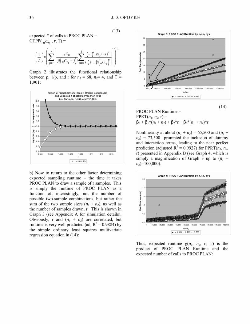
b) Now to return to the other factor determining expected sampling runtime � the time it takes PROC PLAN to draw a sample of r samples. This is simply the runtime of PROC PLAN as a function of, interestingly, not the number of possible two-sample combinations, but rather the sum of the two sample sizes (n1 + n2), as well as the number of samples drawn, r. This is shown in Graph 3 (see Appendix A for simulation details). Obviously, r and (n1 + n2) are correlated, but runtime is very well predicted (adj R2 = 0.9884) by the simple ordinary least squares multivariate regression equation in (14):

Graph 3: PROC PLAN Runtime by n1+n2 by r

0

5

10

15

20

25

30

35

0 200,000 400,000 600,000 800,000 1,000,000 1,200,000 1,400,000

n1+n2

Rea

l Tim

e (s

econ

ds)

r = 1,901 2,700 3,500

(14) PROC PLAN Runtime = PPRT(n1, n2, r) = β0 + β1*(n1 + n2) + β2*r + β3*(n1 + n2)*r Nonlinearity at about (n1 + n2) = 65,500 and (n1 + n2) = 73,500 prompted the inclusion of dummy and interaction terms, leading to the near perfect prediction (adjusted R2 = 0.9927) for PPRT(n1, n2, r) presented in Appendix B (see Graph 4, which is simply a magnification of Graph 3 up to (n1 + n2)=100,000).

Graph 4: PROC PLAN Runtime by n1+n2 by r

0.0

0.5

1.0

1.5

2.0

2.5

0 10,000 20,000 30,000 40,000 50,000 60,000 70,000 80,000 90,000 100,000

n1+n2

Real

Tim

e (s

econ

ds)

r = 1,901 2,700 3,500 Thus, expected runtime g(n1, n2, r, T) is the product of PROC PLAN Runtime and the expected number of calls to PROC PLAN:

( )( ) ( )( ) ( )

1

1 1

1

0

1 !1

! ! ! !

jr i rn n

rn nj T i n n

C j j i

p j C j i j i C

−

= =

− −

= − −

∑ ∑

1n nC


(15) expected runtime = g(n1, n2, r, T) = (14) x (13) = PPRT(n1, n2, r) * CTPP( , r, T) = [ β0 + β1*(n1 + n2) + β2*r + β3*(n1 + n2)*r + d1*β4 + d1*β5*(n1+n2)+ d1*β6*r+d1*β7*(n1+n2)*r + d2*β8+d2*β9*(n1+n2)+d2*β10*r+d2*β11*(n1+n2)*r ] * To get an intuitive feel for r as a function of n1 and n2 (for a given T), note again that the second term of (15) is a combinatorial function of the sample sizes while the first term is merely a linear function of the sample sizes (see Graph 5).

Graph 5: Estimated PROC PLAN Runtime by r (for n1=4, n2=68, and T=1,901 -- based on PPRT in Appendix B)

0.0580

0.0581

0.0582

0.0583

0.0584

0.0585

0.0586

0.0587

0.0588

1,901

1,902

1,903

1,904

1,905

1,9061,907

1,908

1,909

1,910

1,911

1,912

1,913

1,9141,91

51,916

1,917

1,918

1,919

1,920

1,921

r

Estim

ated

Run

time

(sec

onds

)

The combinatorial terms in the second term of (15) end up dominating as sample sizes increase, asymptotically converging to 1.0 (one call to PROC PLAN) faster than the first term (each PROC PLAN runtime) diverges. Hence, for all but very small sample sizes, an optimal r in terms of expected runtime (where ∂g/∂r = 0) will be fairly close to T. Graphs 6 and 7 below present g(n1, n2, r, T) � the product of 1/p in Graph 2 and PPRT in Graph 5 above � and demonstrate an optimal r, r* = 1,908, for T = 1,901, n1 = 4, and n2 = 68 (and ).

Graph 6: Expected Runtime (1/p * each runtime) by r(for n1=4, n2=68, and T=1,901)

0.00

0.05

0.10

0.15

0.20

0.25

0.30

0.35

1,901 1,902 1,903 1,904 1,905 1,906 1,907 1,908 1,909 1,910 1,911 1,912 1,913 1,914 1,915 1,916

r

Expe

cted

Run

time

(sec

onds

)

Graph 7 magnifies the relevant expected runtime range.

Graph 7: Expected Runtime (1/p * each runtime) by r(for n1=4, n2=68, and T=1,901)

0.0582

0.0584

0.0586

0.0588

0.0590

0.0592

0.0594

1,901 1,902 1,903 1,904 1,905 1,906 1,907 1,908 1,909 1,910 1,911 1,912 1,913 1,914 1,915 1,916

r

Exp

ecte

d Ru

ntim

e (s

econ

ds)

Unfortunately, the high level of precision needed to calculate numeric solutions for r* based on (15), for different sample sizes and different values of T, requires use of a symbolic programming language (the Mathematica® v4.1 code used to obtain the exact probabilities in Table 1 is available from the author upon request). Thus, exact solutions cannot be implemented �on the fly� in SAS, or any statistical software package, for encountered values of n1 and n2. Good approximations to the probability mass function of the collector�s problem, however, do exist (see Kuonen (2000) and Read (1998), as well as Lindsay (1992) for a unique approach to the problem), but whether using exact or approximate probabilities, for all practical purposes r* need not be calculated for each and every combination of values of n1 and n2. Nearly optimal r can be calculated for ranges of C because, as shown in Graph 7, the marginal runtime cost of drawing r slightly larger than r* is negligible (though the

r*

1n nC

( )( ) ( )( ) ( )

1

1 1

1

0

1 !

! ! ! !

jr i rn n

rn nj T i n n

C j j i

j C j i j i C

−

= =

− − − −

∑ ∑

1C 1,028,790n nC = =

r*

37 J.D. OPDYKE

marginal runtime cost of drawing r smaller than r* is relatively large). Thus, if we define appropriate ranges of C, and for the lower bound of each range identify r*, these �low-end� r*s always will be larger than any other r* corresponding to any of the sample pairs within their respective ranges. In other words, though not optimal for every combination of sample sizes within its range, the �low-end� r* will be nearly optimal because it will be slightly larger (never smaller) than all other r* for sample size pairs within its range, and the marginal runtime cost of being slightly larger than r* is negligible. Table 1 below shows the values of r used in the permutation test program � the �low-end� r*s � for ranges of C. Although g(n1, n2, r, T) is a function of both C and n1 + n2, and n1 + n2 does vary for (essentially) constant C, the effect of this can be ignored since, as an empirical matter, it never affects the calculation of each of the �low-end� r*s. In other words, CTPP (13) strongly dominates PPRT (14) because 1/p converges to one so quickly. The code in Appendix C proposes an efficient method for generalizing the results from Table 1, i.e. for obtaining estimates of the optimal �low-end� r*s for any value of T. This method is very fast, perhaps even faster than Kuonen (2000), although it provides only estimates to the exact solution. It first utilizes optimal �low-end� r*s already calculated for a particular value of T (as in Table 1) as the basis for conservative estimates of the distance (standard deviations) between a new T and the mean of the collector�s problem mass function. Different r*s are tested via any of several straightforward convergence algorithms (false position converges more quickly than bisection and, surprisingly, Newton-Raphson in this context) to find those r*s yielding distances arbitrarily close to the original conservative distance estimates, typically within just several iterations. The method performs well in practice because of the shape of the runtime function (Graph 7): as long as the original distance estimates are conservative, i.e. slightly larger than necessary, the corresponding estimates of the optimal �low-end� r*s also will be slightly larger than necessary, causing only negligible runtime increases over use of the true optimal �low-end�

r*s. TABLE 1. Nearly Optimal r (�low-end� r*), Probability (p) of T ≥ 1,901 Unique Samples, and Expected # of Calls to PROC PLAN (1/p) by Ranges of # of Sample Combinations, C

C

�low-end�

r*

p (lower bound)

1/p (lower bound)

C < 10,626 C 1.0 (assuming C ≥ T)

1.0

10,626 ≤ C < 52,360

2,138 0.997929320330667

1.002074976280530

52,360 ≤ C < 101,270

1,956 0.999058342955471

1.000942544598290

101,270 ≤ C < 521,855

1,934 0.999429717692296

1.000570607715190

521,855 ≤ C < 1,028,790

1,912 0.999726555240808

1.000273519551680

1,028,790 ≤ C < 10,009,125

1,908 0.999512839120371

1.000487398321020

10,009,125 ≤ C < 25,637,001

1,904 0.999961594180711

1.000038407294350

25,637,001 ≤ C < 100,290,905

1,903 0.999944615376581

1.000055387691050

100,290,905 ≤ C < 5,031,771,045

1,902 0.999839691379204

1.000160334323770

5,031,771,045 ≤ C

1,901 0.999641154940541

1.000358973875460

It is worth noting that, for T = 1,901, the largest value of C for which one has to actually �oversample� (although one must still check for duplicate samples and redraw if necessary) is relatively small � about 5x109. This corresponds to sample sizes of only n1 = 17 and n2 = 18 for small n = n1 + n2, and n1 = 2 and n2 = 100,000 for large n. This is due, of course, to the fantastic combinatorial growth of C, which causes 1/p�s rapid convergence to one. This convergence

1n nC=


indicates that using �oversampling� as outlined above to perform NR sampling should be applicable to any WR sampling procedure, even if its runtime function, unlike (13), is not linear in n (i.e. even if it is convex and steep in n).

Results How Fast Is It? Relative Speed – Some Benchmarks The start-to-finish runtime of the permutation test program using �oversampling� with PROC PLAN to perform NR sampling is fast relative to other programs and WR procedures, as shown below:

Graph 8: Relative Start-to-Finish Runtime (T = 1,901)

19.711.7

2.51.5

0.514.2

7.71.6

1.20.5

1.31.51.4

0.60.2

1.0

12.8

0 1 2 3 4 5 6 7 8 9 10 11 12 13 14 15 16 17 18 19 20

r

q

p

o

n

m

l

k

j

i

h

g

f

e

d

c

b

a

a = PROC PLAN with �oversampling� b = TWOSAMPL, (n1+n2)<10,000, R = 1 c = TWOSAMPL, (n1+n2)<10,000, R > 1 d = TWOSAMPL, 10,000<(n1+n2)<100,000, R = 1 e = TWOSAMPL, 100,000<(n1+n2)<150,000, R=1 f = TWOSAMPL, 1M < (n1+n2) < 1.5M, R = 1 g = TWOSAMPL, 1M < (n1+n2) < 1.5M, R > 1 h = NPAR1WAY, (n1+n2)<10,000, R = 1 i = NPAR1WAY, (n1+n2)<10,000, R > 1 j = NPAR1WAY, 10,000<(n1+n2)<100,000, R = 1 k = NPAR1WAY, 100,000<(n1+n2)<150,000, R=1 l = NPAR1WAY, 1M < (n1+n2) < 1.5M, R = 1 m = MULTTEST, (n1+n2)<10,000, R = 1 n = MULTTEST, (n1+n2)<10,000, R > 1

o = MULTTEST, 10,000<(n1+n2)<100,000, R = 1 p = MULTTEST, 100,000<(n1+n2)<150,000, R=1 q = MULTTEST, 1M < (n1+n2) < 1.5M, R = 1 r = looping in SAS, 1<(n1+n2)<1.5M, R > 1 where R = # Study Groups / # Control Groups (For r above, see Jackson (1998). Beware, however, that this code enters an infinite loop if the number of possible sample combinations for a given sample pair is less than T. Also note that the code, unlike the standard definition of a permutation test which includes �ties� in the numerator of the p-value, splits ties at the boundary after assuming exactly one tie at the boundary (apparently with the intent of making the test less statistically conservative)). The only procedures or programs faster than PROC PLAN with �oversampling� are PROC MULTTEST and PROC NPAR1WAY with small samples and one study group per control group, as well as PROC TWOSAMPL with small samples, regardless of the study-control group ratio. For larger samples, the relative speed of PROC PLAN with �oversampling� over MULTTEST and NPAR1WAY increases rapidly and nonlinearly, even with a study-control group ratio of one. The relative speeds for large samples and larger study-control group ratios (not shown in Graph 8) are many times larger still (note that MULTTEST runtimes reflect only the time required for sample generation, not p-value calculation, which would increase relative runtime by an additional several multiples for larger samples). The relative speed advantage over TWOSAMPL is only pronounced when one sample is large and the study-control group ratio exceeds one. On the one hand, smaller samples are where one is most likely to need permutation tests. However, this is where the speed differential matters the least in absolute terms � even when performing two hundred permutation tests with these smaller sample sizes and a study/control group ratio equal to one, none of the other three procedures was ever more than five minutes faster than PROC PLAN with �oversampling.� So the tradeoff in this case is several minutes per run with MULTTEST, NPAR1WAY, or TWOSAMPL, versus maximum power with PROC PLAN with �oversampling.�

→ 75.8

39 J.D. OPDYKE

In contrast, when samples are larger, relative runtimes matter most because even small differences become large in absolute terms. These are precisely the conditions under which PROC PLAN with �oversampling� maintains a very large relative speed advantage over MULTTEST and NPAR1WAY, as well as TWOSAMPL when the study-control group ratio exceeds one. In addition to the speed of PROC PLAN itself, a number of factors contribute to the speed of the entire SAS program used to perform permutation tests with PROC PLAN and �oversampling,� including: • Use of PROC APPEND to �SET� two large

datasets together (one on top of the other) whenever possible. • Judicious use of multiple PROC

TRANSPOSE�s to evaluate the summarized results of the permutation sampling.

• Most test statistics can be constructed based on just one of the two samples in a pair and, if necessary, the pooled summary statistics of the pair. Thus, when conducting permutation sampling, sample only the smaller of the two samples, but keep track of which sample is used (study or control) when constructing the test statistics based on the permutation samples.

• To quickly SET together the potentially large and numerous output dataset lists from PROC PLAN (one set of T samples for every permutation test), use a looping macro that returns all the dataset names into a single SET statement (see code in Appendix C). Alternately, looping on the SET statement and SETting the datasets together cumulatively, one at a time, is extremely inefficient and

runtime costly. • If the dataset is large and contains a large

percentage of records with the same response variable value (say, zero), delete these records to avoid sorting and later merging them with the PROC PLAN output. After merging the remaining data with the PROC PLAN output

and retaining all PROC PLAN records in the merge, reassign this value to the response variable when it is missing (i.e. when that record did not merge with the PROC PLAN output because it had been deleted).

• Most importantly, if the data contains multiple study groups per control group, there is no need to output control group records multiple times, once for each corresponding study group, when using PROC PLAN with �oversampling.� The original data simply can be divided into two datasets � one for control group(s) and one for study groups � and each merged separately to the PROC PLAN output (then (PROC) APPENDed together after the merges). Unless one constructs a separate dataset for each permutation test, PROC MULTTEST, PROC NPAR1WAY, and PROC TWOSAMPL require control group records duplicated in the input dataset for each study group against which they are being compared. This is what gives PROC PLAN with �oversampling� an additional speed premium in these situations, and similarly, for multiple comparisons. To test a complete null hypothesis under a multiple testing framework, the number of pairwise comparisons required is s (s-1)/2, where s is the number of samples. This means that for the other three procedures, a much larger number of observations (16) must be output and sorted compared to the number similarly processed by PROC PLAN with

�oversampling� (17).

(16)

(17)

where s = the number of samples, and n(i) = the number of observations in the sample with the ith largest number of observations If many permutation tests must be conducted and at least some of these contain large

( ) ( )

1

3 PROCs #obs 1s

i

i

s n=

= − ∑

( ) ( ) ( ) ( )1

2

PROC PLAN #obs 1 1s

s i

i

n s n i−

=

= − −∑


samples, the runtime advantage of (17) over (16) can be extremely large, as seen in Graph 8. However, (17) does not assume the code exploits the fact that with multiple comparisons, the same groups of observations are being used repeatedly in different comparisons. Although the other sampling procedures examined in this study cannot take advantage of this, code based on PROC PLAN can, allowing the researcher to achieve computational efficiencies even beyond those

gained by (17) over (16).

Absolute Speed When run on data containing 220 sample pairs where the smaller sample was less than 30 observations but the larger sample was sometimes as large as 64,000 observations, the runtime of the program was 7 minutes, 45 seconds on a desktop PC with two gigabytes of random-access memory and a two gigahertz Pentium® processor. For data containing 6,682 sample pairs where the smaller sample was less than 30 observations but the larger was sometimes over 5,000,000 observations, the runtime was 8 hours, 36 minutes. The former example obviously is more typical of the contexts in which permutation tests are used, but the latter is instructive for demonstrating the limits of the methods and software being relied upon. This study shows that the runtime of PROC PLAN with �oversampling� is not prohibitive even when applied to sample sizes as large (if not far larger) than would ever be used with permutation tests. The same cannot be said for the four alternate methods. (One notable and widespread example of the current application of permutation tests to sample pairs where one sample can be quite large is the telecommuncations regulatory arena. Incumbent local exchange carriers have been required by a number of state public service commissions to perform permutation tests on performance measurement data if one sample (typically the CLEC sample) is small, even if the other (typically the ILEC sample) contains many millions of observations.)

NR Sampling � How Much Power Gain? The asymptotic approximation of the power differential between NR sampling and WR sampling for a single pairwise comparison is calculated below (Table 2 and Graph 9) based on the Central Limit Theorem ((6.2 � (6.3)). There are two notable findings: first, the power gains from using NR sampling over WR sampling are small, even for small values of δ (the location difference) and , and even taking into consideration that these asymptotic power differences represent lower bounds for the actual power differences. Secondly, these gains decrease rapidly in . Why is this the case? Recall that the only difference between NR sampling and WR sampling is the variance of the estimated p-value; the former is based on the hypergeometric distribution (5.6) and the latter is based on the binomial distribution (5.7).

(5.6)

(5.7) These variances differ only by the finite population correction factor (fpc) of . As n1 and n2 increase, increases dramatically, causing the rapid convergence of the fpc to one and thus, the practical equivalence of NR sampling and WR sampling. Intuitively, this makes sense as it is clear that the probability of drawing any of a few thousand samples (np) more than once quickly approaches zero as the number of possible samples

Permutation Sampling: With (WR) vs. No (NR) Replacement Asymptotic Difference in Power at α = 0.05 by nCn1 by δ

0.00000

0.00005

0.00010

0.00015

0.00020

0.00025

0.00030

0.00035

0.00040

0.00045

0.00050

0 1,000 2,000 3,000 4,000 5,000 6,000 7,000 8,000 9,000 10,000 11,000 12,000 13,000

nCn1 = # Possible Samples

Diff

eren

ce in

Pow

er a

t α =

0.0

5

1,001 Samples Draw n 1,938 3,876 1,001 1,938 3,876

δ = 0.5σ

δ = 1.0σ

( )2 1bin pn p pσ = −

( )( ) ( )1 1

2 1 / 1hyp p n n p n nn p p C n Cσ = − − −

( ) ( )1 1/ 1n n p n nC n C− −

1n nC

1n nC

1n nC

41 J.D. OPDYKE

from which to randomly draw rapidly surpasses trillions and quadrillions of possibilities (the exact probability is given by one minus (12) when T=r). Therefore, if sample sizes are not very small, it is fair to say that such small power gains would only make NR sampling worth considering if there was little or no runtime cost associated with its implementation. Otherwise, unless the cost of Type II error is astronomically high, NR sampling may not be worth the trouble (however, note NR sampling�s more obvious benefit of shorter confidence intervals on the permutation p-values themselves compared to (3), which is based on WR sampling). NR Sampling � Power Gains at What Cost? A good metric for evaluating the runtime cost of employing NR sampling via �oversampling� is its start-to-finish runtime compared to that associated with WR sampling � i.e. just drawing T samples and ignoring the duplicate sample problem. This difference is a function of the number of tests performed and their sample sizes. When only two hundred permutation tests were conducted on small sample pairs (both less than 30 observations), NR sampling was 20%-30% slower than WR sampling. However, in absolute terms, this was less than two minutes. When 1,862 tests were conducted, including some sample pairs with one large sample, the runtime cost was always under 2%; for all 6,682 tests, the runtime cost was always well below 1%. Maximizing power via NR sampling arguably is worth this relatively small increase in runtime.

Conclusion This study provides a) statistical code that performs fast continuous-data permutation tests even if one sample is large, and which often is more than an order of magnitude faster than widely available commercial alternatives under these conditions, and b) an answer to the question: does drawing a set of permutation samples containing no duplicate samples increase the power of the permutation test for a single pairwise comparison? If so, by how much, and are there also power gains for multiple comparisons? It is analytically shown that �no-replacement� (NR) sampling of the permutation sample space provides a small power gain over the usual method of �with-replacement� (WR) sampling when using a conventional Monte Carlo approach (this power gain attains, by definition, maximum power under conventional Monte Carlo). This finding holds for pairwise comparisons, as well as for multiple comparisons � specifically, permutation-style p-value adjustments of permutation test p-values � which are made runtime feasible by an additional speed premium built into the code. The power gain for such multiple comparisons, however, may be larger in absolute terms because these procedures achieve variance reduction from two sources rather than just one. Simulating these gains is the focus of ongoing research. The power gains of both pairwise and multiple comparisons, however, quickly diminish as sample sizes increase. This is due to the rapid convergence of the conditional variance of the estimated permutation p-value (based on the hypergeometric distribution) to that of WR sampling (based on the binomial distribution). However, the runtime cost of implementing NR sampling via the proposed method of �oversampling� is negligible � less than 1% of runtime when many tests are conducted and at least some of the sample pairs contain one large sample (which is when runtime matters most in absolute terms). So under a conventional Monte Carlo approach, if the cost of Type II error is not negligible and even if the power gains of NR sampling may be small, there seems to be no reason not to use this straightforward and readily applied method in order to maximize power.


TABLE 2. Asymptotic Approximation of Power Difference Between NR Sampling vs. WR Sampling for a Pairwise Permutation Test

np 1,001 1,001 1,001 1,938 1,938 3,876

nCn1 2,002 5,005 8,008 3,876 11,628 11,628

(nCn1 - np)/( nCn1

- 1) 0.5002 0.8002 0.8751 0.5001 0.8334 0.6667

aslNR 0.0511734 0.0513080 0.0513416 0.0501677 0.0502451 0.0501290 aslWR 0.0513977 0.0513977 0.0513977 0.0502838 0.0502838 0.0501677 C*

αNR

0.0493837 0.0493128 0.0492950 0.0498490 0.0497793 0.0498968

C*αWR

0.0492655 0.0492655 0.0492655 0.0497445 0.0497445 0.0498658

δ = 0.5 0.5870526 0.6121541 0.6361821 0.7030284 0.7027937 0.7031889 PowerNR δ = 1.0 0.9817270 0.9868391 0.9905697 0.9966619 0.9966550 0.9966665 δ = 0.5 0.5866014 0.6119764 0.6360733 0.7026762 0.7026762 0.7030848 PowerWR δ = 1.0 0.9816750 0.9868234 0.9905623 0.9966516 0.9966516 0.9966635 δ = 0.5 0.0004512 0.0001777 0.0001089 0.0003522 0.0001175 0.0001041 Power

difference δ = 1.0 0.0000520 0.0000157 0.0000073 0.0000103 0.0000034 0.0000030

References

Andersen, M.J. & P. Legendre (1999), An

empirical comparison of permutation methods for tests of partial regression coefficients in a linear model, Journal of Statistical Computation & Simulation, Vol. 62, No. 3.

Berry, K. & P. Mielke (1983), Moment approximations as an alternative to the f test in analysis of variance, British Journal of Mathematical & Statistical Psychology, 36: pp.202-206.

Boos, D., & J. Zhang (June 2000), Monte carlo evaluation of resampling-based hypothesis tests, Journal of the American Statistical Association, Vol. 95, No. 450.

Brown, L., T. Cai, & A. DasGupta, Interval estimation for a binomial proportion, Statistical Science, Vol. 16, No. 2: pp.101-133.

Cochran, W. (1977), Sampling techniques, 2nd ed., New York: John Wiley & Sons.

Evans, M., N. Hastings, & B. Peacock (1993), Statistical distributions, 2nd ed., New York: John Wiley & Sons.

Fisher, Sir R.A. (1935), Design of experiments, Edinburgh, Oliver & Boyd.

Efron, Bradley & Robert Tibshirani (1993), An introduction to the bootstap, Chapman & Hall, London & New York.

Affidavit of John Jackson, On Behalf of MCI-

Worldcom, Before the Michigan Public Service Commission, Case No. U-11830, November 18, 1998, ATTACHMENT A, �Using Permutation Tests to Evaluate the Significance of CLEC vs. ILEC Service Quality Differentials�

Kuonen, D. (August 2000), A saddlepoint approximation for the collector�s problem, The American Statistician, Vol. 54, No. 3.

Lindsay, J.D. (1992), A new solution for the probability of completing sets in random sampling: definition of the �two-dimensional factorial�, The Mathematical Scientist, 17: 101-110.

Mehta, C., & N. Patel (June 1983), A network algorithm for performing fisher�s exact test in r x c contingency tables, Journal of the American Statistical Association, Vol. 78, No. 382.

Mielke, P. & K. Berry (2001), Permutation methods: a distance function approach, Springer-Verlag, New York.

Naiman, D. & C. Priebe (2001), Computing scan statistic p values using importance sampling, with applications to genetics and medical image analysis, Journal of Computational and Graphical Statistics, Vol. 10, No. 2.

43 J.D. OPDYKE

Opdyke, J.D. (May 5-8, 2002a), PharmaSUG2002: Conference of the Pharmaceutical SAS Users� Group, Salt Lake City, UT, http://www.pharmasug.org/psug2002/bp2002/ psug2002_html

Opdyke, J.D. (August 5-7, 2002b), MCP 2002: The 3rd International Conference on Multiple Comparisons, Bethesda, Maryland, http://www.ba.ttu.edu/isqs/westfall/Program.htm

Ortiz, L. & L. Kaelbling (2000), Sampling methods for action selection in influence diagrams, Proceedings of the Seventeenth National Conference on Artificial Intelligence.

Owen, A. & Y. Zhou (March 2000), Safe & effective importance sampling, Journal of the American Statistical Association, Vol. 95, No. 449.

Pesarin, F. (2001), Multivariate permutation tests with applications in biostatistics, John Wiley & Sons, Ltd., New York.

Read, K.L.Q. (May 1998), A lognormal approximation for the collector�s problem, The American Statistician, Vol. 52, No. 2.

Westfall, P., & S. Young (1993), Resampling-based multiple testing – examples & methods for p-value adjustment, New York, John Wiley & Sons, Inc.

Appendix A

To estimate PROC PLAN real runtime,

SAS® v.8.2 was used on a desktop PC with 2GB RAM and a 2GHz Pentium processor. Sample sizes were generated by assigning values of 3, 16, and 27 to the smaller of the two samples, and, beginning at 100, assigning values by 100 increments to the larger sample up to 100,000, after which point increments of 10,000 were used up to 1.5 million (though the program has been run on sample pairs as large as 29 and 5,000,029). Three values of r were used: 1,901, 2,700, and 3,500.

Appendix B

PROC PLAN RunTime, PPRT(n1, n2, r), regression results: Left hand side variable = real runtime seconds adjusted R2 = 0.9927

Variable Key Variable

A Intercept B (n1 + n2) C r D (n1 + n2) * r E [(n1 + n2) < 65.5K] F [(n1 + n2) < 65.5K] * (n1 + n2) G [(n1 + n2) < 65.5K] * r H [(n1 + n2) < 65.5K] * (n1 + n2) * r I [65.5K £ (n1 +n2) £ 73.5K] J [65.5K £ (n1 +n2) £ 73.5K] * (n1 + n2) K [65.5K £ (n1 +n2) £ 73.5K] * r L [65.5K £ (n1 +n2) £ 73.5K] * (n1 + n2) * r

Variable Key Parameter Estimate t value

A 0.0432387277000000 1.80B -0.0000001298032000 -2.88C 0.0000838185000000 9.68D 0.0000000038095955 234.72E -0.0340413560000000 -0.89F 0.0000004543242500 0.58G -0.0000581740000000 -4.24H -0.0000000024994500 -8.86I -0.4873557050000000 -0.38J 0.0000071862352000 0.39K -0.0016941670000000 -3.70L 0.0000000228154240 3.47


Appendix C

options = nomprint nomlogic nomrecall; %MACRO RUN_PRG; *** the By Variables and npermsampT normally would be passed in the main macro (RUN_PRG).; %let byvars=byvar1 byvar2 byvar3 byvar4 byvar5; *** npermsampT = # of permutation samples; %let npermsampT=1901; *** count the number of byvars for parsing; %let byvars=%cmpres(&byvars); %let num_byvars= %eval(%length(&byvars)- %length(%cmpres(&byvars))+1); *** summarized data (SUMDINPT) contains study group identifier (stdy), control group identifier (cntl), # study group obs, # control group obs, and any By Variables.; %let noconverge=0; data sumdinpt(keep=combins nsamp minrcomb minof3 bigcomb ncalls2pp topdraws lastdraw smaller nobsmalr studynobs contrlnobs sumofnobs stdy cntl &byvars); set sumdinpt; *** create variables to be passed to CREATSMP, which generates the permutation samples corresponding to each record on SUMDINPT; if "&npermsampT"="1901" then maxcombins=5031771045; else maxcombins=9*10**16; *** for versions of SAS v6.12 and older, comb(,) terminates for results of approximately 10E70 and higher, so use the loop below instead; if ("&sysver"*1)<8 then do; combins=1; minnobs=min(studynobs,contrlnobs); bothnobs=sum(studynobs,contrlnobs); do j=minnobs to 1 by -1; combins=combins*(bothnobs-j+1)/j; if combins>maxcombins then goto enufcomb; end; enufcomb: combins=round(combins); end; else do; combins=comb(sum(studynobs,contrlnobs), min(studynobs,contrlnobs)); *** if still too large, assign large number; if combins=. then combins=maxcombins; end;

*** The 'table' below was calculated based on the exact probabilities of the Collectors Problem distribution and presents the optimal "low-end" sample sizes by ranges of nCn1 (p.7 above) only for npermsampT = 1901.; IF “&npermsampT” = “1901” THEN DO; if combins<&npermsampT then nsamp=&npermsampT; else if combins<10626 then nsamp=combins; else if combins<52360 then nsamp=2138; else if combins<101270 then nsamp=1956; else if combins<521855 then nsamp=1934; else if combins<1028790 then nsamp=1912; else if combins<10009125 then nsamp=1908; else if combins<25637001 then nsamp=1904; else if combins<100290905 then nsamp=1903; else if combins<5031771045 then nsamp=1902; else if combins>=5031771045 then nsamp=1901; END; *** For npermsampT other than 1901, obtain nsamp with a convergence routine based on the first and second moments of the Collectors Problem distribution and using the nsamp calculated above as a basis for the starting values. Even for large npermsampT (e.g. 32,000) and conservatively defined Xstdev, convergence (based on false position) typically is achieved in less than five iterations; ELSE DO; *** Define X*stdev (Xstdev) here conservatively, based on the size of npermsampT compared to 1901 (the base would be Xstdev = 2.875 since this is (approximately) true when npermsampT = 1901). Larger npermsampT allows for the use of smaller Xstdev, but smaller npermsampT requires larger Xstdev to maintain the same (approximate) probability of a redraw. Any functional relationship between Xstdev and npermsampT similar to the one below can be used (the exponent below (0.25) was chosen based on a wide range of values for npermsampT).; Xstdev= (1901/&npermsampT)**0.25; if combins<&npermsampT then startratio=-999; else if combins<(&npermsampT*10626/1901) * Xstdev then startratio=-888; else if combins<(&npermsampT*52360/1901) * Xstdev then startratio=2138/1901; else if combins<(&npermsampT*101270/1901) * Xstdev then startratio=1956/1901; else if combins<(&npermsampT*521855/1901) * Xstdev then startratio=1934/1901; else if combins<(&npermsampT*1028790/1901) * Xstdev then startratio=1912/1901; else if combins<&npermsampT*10009125/1901 * Xstdev then startratio=1908/1901; else if combins<&npermsampT*25637001/1901 * Xstdev then startratio=1904/1901;

45 J.D. OPDYKE

else if combins<&npermsampT*100290905/1901 * Xstdev then startratio=1903/1901; else if combins<&npermsampT*5031771045/1901 * Xstdev then startratio=1902/1901; else if combins>=&npermsampT*5031771045/1901 * Xstdev then startratio=1.0; IF startratio=-999 | startratio=1 THEN nsamp=&npermsampT; ELSE IF startratio=-888 THEN nsamp=combins; ELSE IF startratio>1 THEN DO; *** Starting value for nsamp.; nsamp=ceil(startratio*&nresamp); nsampoldhigh=nsamp; nsampoldlow=(&nresamp*1); initgap=nsampoldhigh-nsampoldlow; colldist_avg = combins*(1- (1-1/combins)**nsampoldlow); *** Numeric precision constraints prevent calculation of the second moment for large inputs, but a conservative (i.e. larger-than-actual) approximation suffices in these cases.; if (combins*(combins-1)* (1- 2/combins)**nsampoldlow) > 100144465758007 then colldist_stdev = 0.4; else colldist_stdev = sqrt(combins*(combins-1)* (1-2/combins)**nsampoldlow+ combins*(1-1/combins)**nsampoldlow- combins**2*(1-1/combins)** (2*nsampoldlow)); lowpoint =(colldist_avg – Xstdev * colldist_stdev - &nresamp*1); colldist_avg = combins*(1- (1-1/combins)**nsampoldhigh); if (combins*(combins-1)* (1- 2/combins)**nsampoldhigh) > 100144465758007 then colldist_stdev = 0.4; else colldist_stdev = sqrt(combins*(combins-1)* (1-2/combins)**nsampoldhigh+ combins*(1-1/combins)**nsampoldhigh- combins**2*(1-1/combins)** (2*nsampoldhigh)); highpoint = (colldist_avg – Xstdev * colldist_stdev-&nresamp*1); point=highpoint; *** Use counter only to eliminate the possibility of infinite loop.; DO z=1 to 1000; *** Obtain nsamp only to within 4 of optimal nsamp (when converging on nsamp from upper

bound) to prevent unnecessary looping.; TOPLOOPNSAMP: if point>4 then do; nsampoldhigh=nsamp; nsamp=ceil((nsampoldlow * highpoint – nsampoldhigh * lowpoint) / (highpoint-lowpoint)); end; *** If necessary, get upper bound above zero on 1st loop (& increment lower bound concurrently); else if z=1 & point<-1 then do y=1 to 1000; nsampoldlow = nsamp; nsamp = ceil(nsamp+initgap); colldist_avg = combins*(1- (1-1/combins)**nsamp); if (combins*(combins-1)* (1- 2/combins)**nsamp) > 100144465758007 then colldist_stdev = 0.4; else colldist_stdev = sqrt(combins*(combins-1)* (1-2/combins)**nsamp+ combins*(1-1/combins)**nsamp- combins**2*(1-1/combins)** (2*nsamp)); highpoint = (colldist_avg - Xstdev * colldist_stdev - &nresamp*1); point = highpoint; if point>4 then do; colldist_avg = combins*(1- (1-1/combins)**nsampoldlow); if (combins*(combins-1)* (1- 2/combins)**nsampoldlow) > 100144465758007 then colldist_stdev = 0.4; else colldist_stdev = sqrt(combins*(combins-1)* (1-2/combins)**nsampoldlow+ combins* (1-1/combins)**nsampoldlow- combins**2*(1-1/combins)** (2*nsampoldlow)); lowpoint = (colldist_avg - Xstdev*colldist_stdev - &nresamp*1); goto TOPLOOPNSAMP; end; else if -1<=point<=4 then goto STOPCNVG; end; *** Require a stricter convergence criterion on optimal nsamp when converging from lower bound;


else if point<-1 then do; nsampoldlow=nsamp; nsamp=ceil((nsampoldlow*highpoint – nsampoldhigh*lowpoint) / (highpoint-lowpoint)); end; else if -1<=point<=4 then goto STOPCNVG; if z = 1000 then do; noconverge = 1; goto STOPCNVG; end; *** For next iteration; temp_avg = combins* (1-(1-1/combins)**nsamp); if (combins*(combins-1)* (1- 2/combins)**nsamp) > 100144465758007 then temp_stdev = 0.4; else temp_stdev = sqrt(combins*(combins-1)* (1-2/combins)**nsamp + combins*(1- 1/combins)**nsamp - combins**2* (1-1/combins)**(2*nsamp)); temp_point = (temp_avg - Xstdev * temp_stdev - &nresamp*1); if temp_point >= 0 then do; highpoint = temp_point; point = highpoint; end; else do; lowpoint = temp_point; point = lowpoint; end; END; STOPCNVG: if noconverge = 1 then do; call symput('noconverge', compress(noconverge)); stop; end; END; END; minrcomb=min(combins,nsamp); minof3=min(combins,nsamp,&npermsampT); if combins=minrcomb then bigcomb=0; else if combins>minrcomb then bigcomb=1; ncalls2pp=ceil(minrcomb* sum(studynobs,contrlnobs)/2**31); topdraws=floor(nsamp/ncalls2pp); lastdraw=topdraws+mod(nsamp,ncalls2pp); if studynobs<=contrlnobs then smaller="stdy"; else smaller="cntl";

nobsmalr=min(studynobs,contrlnobs); sumofnobs=sum(studynobs,contrlnobs); run; *** Although algorithm should always converge, code should account for any contingency.; %if &noconverge=1 %then %do; %put; %put WARNING: The permutation sample-size algorithm did not converge.; %put Scrutinize the data and/or adjust the functional relationship between Xstdev and npermsampT.; %put; %goto EXITALL; %end;

*** define outside of CREATSMP (which is called in a loop) four macros used for assigning By Variables and their values (exactly as they exist on both the original data (FULLDATA) and SUMDINPT) to the sampling datasets generated by PROC PLAN in CREATSMP; %MACRO GETVARLEN(varname=); %let dsetid=%sysfunc(open(fulldata)); %let len=%sysfunc(varlen(&dsetid, %sysfunc(varnum(&dsetid,&varname)))); %let dsetid=%sysfunc(close(&dsetid)); &len %MEND GETVARLEN; %MACRO ASSIGNBYVRLENS; %do p=1 %to &num_byvars; &&byvar&p $%GETVARLEN(varname=&&byvar&p) %end; %MEND ASSIGNBYVRLENS; %MACRO ASSIGNBYVRVALS; %do q=1 %to &num_byvars; %let x=%scan(&byvars,&q,' '); %str(&x=resolve("&"||"&x");) %end; %MEND ASSIGNBYVRVALS; %MACRO GETBYVARVALUES; %do q=1 %to &num_byvars; %let x=%scan(&byvars,&q,' '); %str(byvarval=resolve("&"||"&x"); output;) %end; %MEND GETBYVARVALUES; *** When multiple loops on PROC PLAN required...; *** ...use for combining datasets.; %MACRO COMBBIGSAMPS; %do s=2 %to &ncalls2pp; ptemp&s.(in=in&s) %end; %MEND COMBBIGSAMPS; *** ...use for assigning DRAWNUM values.; %MACRO ASSIGNDRAWNUM;

47 J.D. OPDYKE

%if &ncalls2pp>2 %then %do k=3 %to &ncalls2pp; %str(else if in&k then drawnum = drawnum+(&k-1)*&topdraws;) %end; %MEND ASSIGNDRAWNUM; *** Obtains # of records in a dataset.; %MACRO NOBS(dset); %if %sysfunc(exist(&dset)) %then %do; %let dsid=%sysfunc(open(&dset)); %let nobs=%sysfunc(attrn(&dsid,nobs)); %let dsid=%sysfunc(close(&dsid)); %end; %else %let nobs=0; &nobs %MEND NOBS; %let seednum =-1; %MACRO CREATSMP(recountr = ); *** The automatic random seed for PROC PLAN, based on the time of day, does not update as fast as PROC PLAN is repeatedly called in the loops below. Hence, ranuni() is used to generate the seed, & its value is explicitly checked to ensure the current random number is different from the previous one. This ensures random sampling is unrelated across tests.; *** if combins <= r, choose all sample combinations, then select npermsampT samples from them.; %if &bigcomb=0 %then %do; data _null_; x=1000000000*ranuni(-1); if compress(&seednum)=compress(" "||x) then x=x+1; call symput('seednum',compress(x)); run; %if &nobsmalr=1 %then %do; proc plan seed=&seednum; factors drawnum = 1 dataobsid = &minof3 of &combins random / noprint; output out = psamp&recountr; run; %end; %if &nobsmalr>1 %then %do; *** cannot just select first npermsampT draws because the comb option orders them, and the data may be ordered in some way; proc plan seed=&seednum; factors drawnum = &combins dataobsid =&nobsmalr of &sumofnobs comb / noprint; output out = psamp&recountr; run;

%if &combins>&npermsampT %then %do; data _null_; x=1000000000*ranuni(-1); if compress(&seednum)= compress(" "||x) then x=x+1; call symput('seednum',compress(x)); run; proc plan seed=&seednum; factors drawnum = 1 dataobsid=&npermsampT of &combins random / noprint; output out = choosmp; run; data choosmp(keep=drawnum); set choosmp(drop=drawnum); drawnum=dataobsid; run; proc sort data=choosmp; by drawnum; run; proc sort data=psamp&recountr; by drawnum; run; data psamp&recountr; merge psamp&recountr choosmp(in=inchoos); by drawnum; if inchoos then output psamp&recountr; run; data psamp&recountr(drop=drawnum2); set psamp&recountr(drop=drawnum); retain drawnum2 0; if mod(_n_,&nobsmalr)=1 then drawnum2 = drawnum2+1; drawnum=drawnum2; run; %end; %end; %end; *** if combins > r, check whether PROC PLAN needs to be looped multiple times -- if not, simply select r samples, delete duplicates, and keep npermsampT samples. If so, loop it first to select r samples. In either case, redraw samples if fewer than npermsampT unique samples are drawn the first time around.; %if &bigcomb=1 %then %do; %redraw1: data _null_; x=1000000000*ranuni(-1); if compress(&seednum)= compress(" "||x) then x=x+1; call symput('seednum',compress(x)); run; %if &ncalls2pp=1 %then %do;


proc plan seed=&seednum; factors drawnum = &minrcomb dataobsid= &nobsmalr of &sumofnobs random / noprint; output out = psamp&recountr; run; proc sort data=psamp&recountr; by drawnum; run; proc transpose data=psamp&recountr out=temp prefix=stdy; var dataobsid; by drawnum; run; proc sort data=temp out=temp nodupkey; by stdy1-stdy&nobsmalr; run; %let ndrawn=%nobs(temp); %if &ndrawn < &npermsampT %then %do; %put; %put Fewer than &npermsampT unique permutation samples (only &ndrawn) were drawn in a &sumofnobs-choose-&nobsmalr draw; %put for the study - control group pair and "by variable" values listed below:; %put ====================================; %put Study Control &byvars; data holdvals; %GETBYVARVALUES run; proc sql noprint; select byvarval into :byvarvals separated by ' ' from holdvals; quit; proc datasets library=work nolist; delete holdvals temp; run; %put &stdy &cntl &byvarvals; %put; %put A redraw has been performed.; %put; %goto redraw1; %end; %else %do; proc datasets library=work nolist; delete temp; run; %if &ndrawn>&npermsampT %then %do; data psamp&recountr; set psamp&recountr (where=(drawnum<=&npermsampT)); run;

%end; %end; %end; %redraw2: %if &ncalls2pp>1 %then %do q=1 %to &ncalls2pp; %if &q<&ncalls2pp %then %do; data _null_; x=1000000000*ranuni(-1); if compress(&seednum)=compress(" "||x) then x=x+1; call symput('seednum',compress(x)); run; proc plan seed=&seednum; factors drawnum = &topdraws dataobsid = &nobsmalr of &sumofnobs random / noprint; output out = ptemp&q; run; %end; %if &q=&ncalls2pp %then %do; data _null_; x=1000000000*ranuni(-1); if compress(&seednum)= compress(" "||x) then x=x+1; call symput('seednum',compress(x)); run; proc plan seed=&seednum; factors drawnum = &lastdraw dataobsid = &nobsmalr of &sumofnobs random / noprint; output out = ptemp&q; run; data psamp&recountr; set ptemp1 %COMBBIGSAMPS; if in2 then drawnum=drawnum+&topdraws; %ASSIGNDRAWNUM run; proc sort data=psamp&recountr; by drawnum; run; proc transpose data=psamp&recountr out=temp prefix=stdyn; var dataobsid; by drawnum; run; proc sort data=temp out=temp nodupkey; by stdyn1-stdyn&nobsmalr; run; %let ndrawn=%nobs(temp); %if &ndrawn < &npermsampT %then %do; %put; %put Fewer than &npermsampT unique permutation samples (only &ndrawn) were drawn in a &sumofnobs-choose-&nobsmalr draw;

49 J.D. OPDYKE

%put for the study - control group pair and "by variable" values listed below:; %put ==================================; %put Study Control &byvars; data holdvals; %GETBYVARVALUES run; proc sql noprint; select byvarval into :byvarvals separated by ' ' from holdvals; quit; proc datasets library=work nolist; delete holdvals temp; run; %put &stdy &cntl &byvarvals; %put; %put A redraw has been performed.; %put; %goto redraw2; %end; %else %do; proc datasets library=work nolist; delete temp; run; %if &ndrawn>&npermsampT %then %do; data psamp&recountr; set psamp&recountr (where=(drawnum<=&npermsampT)); run; %end; %end; %end; %end; %end; *** assign By Variable values on the sampling datasets generated by PROC PLAN in CREATSMP.; data psamp&recountr; length %ASSIGNBYVRLENS; set psamp&recountr; %ASSIGNBYVRVALS run; %MEND CREATSMP; *** In a loop, generate permutation samples for each record of SUMDINPT.; %let sumdsid=%sysfunc(open(sumdinpt)); %let topofloop=%sysfunc(attrn(&sumdsid,nobs)); %syscall set(sumdsid); %do i=1 %to &topofloop; %let fo=%sysfunc(fetchobs(&sumdsid,&i)); %CREATSMP(recountr=&i); %end; %let sumdsid=%sysfunc(close(&sumdsid));

*** After looping above, combine PROC PLAN output datasets to merge with the original unsummarized dataset (FULLDATA) by By Variables & record id variable (dataobsid). Use the variable “smaller” when calculating the test statistic for every permutation sample.; %MACRO COMBSAMPS; %do i=1 %to &totsamps; psamp&i %end; %MEND COMBSAMPS; data samples; set %COMBSAMPS; run; proc datasets library=work nolist; delete %COMBSAMPS; run; %EXITALL: %MEND RUN_PRG; %RUN_PRG;

Documents

REGULAR ARTICLES Fast Permutation Tests that …. Opdyke - JMASM Vol2 No1.pdf · REGULAR ARTICLES Fast Permutation Tests that Maximize Power Under Conventional Monte Carlo Sampling