Embed Size (px)
Citation preview
REGRESSION-BASED TESTS OF PREDICTIVE ABILITY
Kenneth D. West
Michael W. McCracken
July 1995Last revised January 1998
We thank Frank Diebold, Neil Ericcson, Art Goldberger, Matthew Higgens,Yuichi Kitamura, three anonymous referees and seminar participants at the 1996Midwest Economics Association Meetings, the Federal Reserve Board ofGovernors, the University of Maryland and the University of Wisconsin forhelpful comments, and the National Science Foundation and the Graduate Schoolof the University of Wisconsin for financial support.
ABSTRACT
We develop regression-based tests of hypotheses about out of sample
prediction errors. Representative tests include ones for zero mean and zero
correlation between a prediction error and a vector of predictors. The
relevant environments are ones in which predictions depend on estimated
parameters. We show that standard regression statistics generally fail to
account for error introduced by estimation of these parameters. We propose
computationally convenient test statistics that properly account for such
error. Simulations indicate that the procedures can work well in samples of
size typically available, although there sometimes are substantial size
distortions.
Kenneth D. WestDepartment of Economics7458 Social Science BuildingUniversity of Wisconsin1180 Observatory DriveMadison, WI 53706-1393and NBER
Michael W. McCrackenDepartment of Economics6473A Social Science BuildingUniversity of Wisconsin1180 Observatory DriveMadison, WI [email protected]
1. Introduction
In this paper, we develop and simulate regression tests for properties of
out of sample prediction errors. Examples of such properties are: zero mean,
zero serial correlation (if the prediction is one-step ahead), zero correlation
with the prediction, and zero correlation with the prediction from another,
non-nested model. Empirical papers that examine these or related properties
include Mincer and Zarnowitz (1969), Nelson (19721, Howrey et al. (19741,
Berger and Krane (1985), Meese and Rogoff (1983, 19881, Akgiray (19891, Diebold
and Nason (1990), Fair and Shiller (1990), Pagan and Schwert (1990), West and
Cho (1995) and some of the participants in the Makridakis (1982) competition.
If the predictions do not depend on estimated parameters, it follows from
Diebold and Mariano (1996) that under mild conditions standard regression
statistics may be used. For zero serial correlation in one step ahead
prediction errors, for example, one can simply regress the period t+l
prediction error on the period t prediction error, and use a standard t-test to
test the null that the coefficient is zero.
But if the predictions do depend on estimated parameters, the results of
Diebold and Mariano (1996) need not apply. The usual tests do account for
uncertainty that would be present if (counterfactually) the underlying
parameter vector were known rather than estimated, but ignore uncertainty
resulting from error in estimation of that parameter vector. Using a
conventional set of assumptions, we establish conditions under which this
second type of uncertainty is asymptotically negligible, thereby validating the
Diebold and Mariano (1996) procedure. More importantly, we show that such
uncertainty sometimes is asymptotically non-negligible, and then suggest
computationally convenient ways to obtain test statistics that account for both
types of uncertainty. Simulations indicate that failure to account for the
second type of uncertainty sometimes results in poorly sized hypothesis tests,
while our own adjusted tests usually but not always yield more accurately sized
tests.
A vast literature has considered predictive accuracy. A distinguishing
element of our work is explicit consideration of the role of estimation of
parameters needed for prediction. We focus on test statistics produced by
L .
regression packages. These have appeared in a number of applied papers (e.g.,
Fair and Shiller (1990))‘ Pagan and Schwert (1990)), and, we hope, may appear
in still more papers upon development of techniques such as those proposed
here.l We build on earlier work (especially West (1996)) not only by
developing computationally convenient procedures, but also by allowing
additional sampling schemes (additional ways of dividing available data into
estimation and prediction components), relaxing certain technical conditions
that implicitly ruled out certain important tests (including zero correlation
between a prediction error and a prediction), and supplying new simulation
evidence.
Section 2 of the paper describes the environment. Sections 3 and 4
present technical assumptions and basic asymptotic results. Section 5 presents
our computationally convenient adjustments to standard regression statistics.
Sections 6 and 7 specialize sections 3-5 to consider some common tests, when
the underlying models are linear and exactly identified. Section 8 presents
simulation evidence. Section 9 concludes. The Appendix presents proofs. An
additional appendix available on request from the authors presents details of
proofs and simulation results omitted from the paper to save space.
2. Description of Environment
Let 721 be the prediction horizon of interest. There are P Eredictions
in all, which rely on estimates of a (kxl) unknown parameter vector /3'. To
avoid certain singularities we assume ks0 and merely note that our results
specialize in the obvious way when regression estimates are not required to
make predictions.
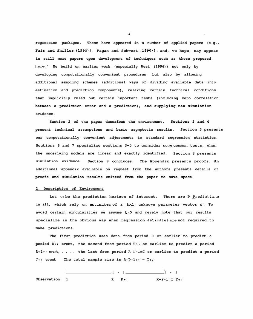
The first prediction uses data from period R or earlier to predict a
period R+T event, the second from period R+l or earlier to predict a period
R+l+r event, . . . . the last from period R+P-l=T or earlier to predict a period
T+T event. The total sample size is R+P-l+r = T+T:
I
Observation: 1
I - I II - I
R R+T R+P-l=T T+r
3
In estimating fl', three different schemes to use available data are
prominent in the forecasting literature. We consider the three explicitly
because results vary for the three. The first scheme, which we call recursive,
was used by, for example, Fair and Shiller (1990). This scheme uses all
available data, estimating ~3' first with data from 1 to R, next with data from
1 to R+l, . . . , and finally with data from 1 to T. The second scheme, which we
call rollinq, was used by, for example, Akgiray (1989). This scheme fixes the
sample size, say at R, and drops distant observations as recent ones are added.
Thus, p' is estimated first with data from 1 to R, next with data from 2 to
R+l, . . . , and finally with data from P to T. The third and final scheme,
which we call fixed, was used by, for example, Pagan and Schwert (1990). This
scheme estimates /3' just once, say on data from 1 to R, and uses the estimate
in forming all P predictions; data realized subsequent to R are, however, used
in forming predictions, as described in the previous paragraph and below.
For t=R,... ,T, let 2, be the regression vector used for prediction when
data from period t and earlier are used. In the least squares model
yt=X,' P'+u, 8 for example, 2, is estimated using
(2.1) data from 1 to t in the recursive scheme, &= (Et x x ' ) -?c~.lx,y,,S-1 8 s
data from t-R+1 to t in the rolling scheme, k= (~LR+lXs%' ) ‘lc&R+lXsYsr
data from 1 to R in the fixed scheme, &= e:&x,' 1 -l~:,,x,y,~
Note that for the fixed scheme, 2, is the same for all t, and depends only on R
and not t, while in the recursive and fixed scheme a different regression
estimate is used for each t. As well, for the rolling and fixed schemes, IL
should properly be subscripted >t,R; the dependence on R is suppressed for
notational simplicity. The asymptotic approximation assumes that both P and R
are large (formally, P,R --, w), with T fixed.
One is interested in the relationship between a scalar prediction error
and a vector of variables--say, whether the prediction error is correlated with
the vector of variables. As illustrated in example 2 below, we can limit the
formal discussion to prediction errors and still yield results applicable to
inference about predictions as well; given the linearity of the procedures we
4
analyze, results for predictions ( = observed data point - prediction error)
follow immediately. We limit the formal analysis to a scalar dependent
variable to economize on notation; we comment occasionally on vector
generalizations of our results.
Let vt+, (0') sttr be the scalar prediction error of interest, with v,,,($,) 3A A AV t.t+r (v t+1 = vt,t+l)the corresponding random variable evaluated at 2,. As the
dating suggests, v~+~ typically relies on data realized in period t+T. One is
interested in the linear relationship between vt+, and a vector function of
period t data. Let 4t+l (P') =g,+, denote this (Pxl) vector function, with g,+,(;,)
= &+1 the sample counterpart evaluated at 2,. In most applications P is
small, say P=l or P=2. Here, g,+, (8') depends on data observed in period t and
earlier; the dating convention is used because g,+, often depends on the
predetermined variables available at time t+I. See the examples below.
The aim is to use a least squares regression to test the null hypothesis
that Ev g -0.t+r t+1- The obvious regression is one of hVt,t+, on Gt+l for
t=R, . . . . R+P-1, obtaining
(2.2) R.t+r = Gt+,# 2 + “;,+,t 2. = (&t+l$t+l# 1 -l&t+l:t,t+T, ;,+, = hVt.t+r-;;t+lt 2.
One then uses the estimate of 2 and a suitable variance-covariance matrix to
test the null.
To illustrate, here are four examples, illustrated with the simple zero
mean AR(l) model Y~=/~'Y~.~+u~, lfl'\<l.
1. Mean prediction error. Here, g,+,=l is a scalar. If Vt+r is a T step ahead
forecast error in the AR(l) model, then St,t+7=yt+, -kYt.
2. Efficiency. Here, one regresses yt+r on the period t prediction (=z;y,, in
the AR(l) model) and perhaps a constant and other possible predictors as well.
The null is that the coefficient on the prediction is unity, on any other
included variables is zero. To analyze this regression using our framework,
which presumes that the dependent variable is a prediction error, note that if
one uses the prediction error (=yt+,- &Yt in the AR(l) model) as the dependent
variable the regression results are algebraically identical to those with yt+7
on the left hand side, except that the estimated coefficient on the prediction
5A
will be smaller by unity. Hence, for say T=l, if g,,, is (2x1) and includes a
constant term as well as ijtyt,A
H, is rr=(O,O)'. Note the dating convention: g
is dated t+l, but depends on yt, the regressor available for prediction at time
t+1.
3. Encomoassinq. Here, v~+~ is a one step ahead forecast error from a
putatively encompassing model. The right hand side variable Gt+L is the scalar
prediction from a putatively encompassed model, and the null is cr=O. More
generally, the right hand side might include a constant in which case $t+l and
CY are (2x1) and the null is cy=(O,O)'.
4. Serial correlation. If Vt+1 is the 1 step ahead forecast error in a model
presumed to have serially uncorrelated errors (=u~+~ in the AR(l) model), thenA
9t+1=vt is the previous period's forecast error. So Q is a scalar, o an
estimate of the first order serial correlation coefficient, and H, is CY=O.~
One of our major aims is to develop computationally convenient
procedures, which in our regression context means using standard errors
produced by standard computer programs, or perhaps simple adjustments to those
standard errors. As we shall see, conventional test statistics are not always
asymptotically valid, even when ~=l and v~+~=~~+~(P') is a zero mean iid variable
that is independent of gt+l=gt+l(P*) . The reason is that in some applications,
two sources of uncertainty affect asymptotic inference about (Y. The first is
uncertainty that would be present even if (counterfactually) p* were known and
one could regress vttr on g,+,. The second results from use of $, rather than
the unknown p'. According to our asymptotic approximation, standard regression
statistics properly account for the first source of uncertainty but not
necessarily the second. We show below that in some important examples,
properly accounting for both sorts of uncertainty requires merely resealing the
least squares variance-covariance matrix by a certain function of P/R.
When such a simple adjustment does not suffice, one can sometimes obtain
asymptotically valid test statistics by auqmentinq the regression (2.2) with a
judiciously chosen set of variables $2t+l. In this case, one runs the
regression

6
(2.3) ^v,,,+, = $t+I'~ + $It+l'~, + disturbance = $t+ltz + disturbance,
where $ 2t+l is a (rxl) set of extra variables included so that conventionally
computed hypothesis tests on cy are correctly sized accordingly to our
asymptotic theory; $ = (&+IJr$2t+lT is (P+r)xl; g,+, = &+,(p*) =
(9,+, (0') ' t92,+, (P') ‘ 1 ' = (9t+1' ,92t+1’ )' and G are also (Q+r) xl.
3. Assumptions
This section presents assumptions relevant for the basic regression
( 2 . 2 ) ; section 5 will present an extension for analysis of the augmented
regression (2.3). Our assumptions are "high level" ones. We use relatively
abstract assumptions for two reasons. First, they allow us or others to verify
that our results apply to tests and models other the ones we consider in detail
in sections 6 and 7 below. Second, they can be presented compactly. In the
interest of concision and clarity, we also do not attempt to state each theorem
using a minimal set of assumptions. For example, a weaker version of
assumption 3 applies in applications with parametric covariance matrix
estimators.
Some notation: for any differentiable function n,:R" + R" and for x in the
domain of n,, axtit denotes the (sxm) matrix of partial derivatives of n,; for any
function n, whose domain is in Rk, ntB 3 at(p*);afi
for any matrix A = [aijl, let
I Al I I= maxi,jIaij,; summations of variables indexed by t or t+T run from t=R to
t=T=R+P-1: for any variable x, Xx(t) = xT*Rx(t), &+r = CT xt-R t+r; summations of
variables indexed by s run from (a)1 to t, for the recursive scheme, (b)t-R+l
to t, for the rolling scheme, (c)l to R, for the fixed scheme: for any variable
x, (a)Ex, = XiX1x, (recursive), (b)Cx, = E:=t.R+l~s (rolling), (c)X,x, = CR xs-1 B
(fixed). Finally, let
(3.1) f,+,(P') = g,+,(P')v,+,(P*) , ft+,,o = =*,(P*) Iw
F = Ef,,,,,.
Here, ft+,:Rk -P R'; the (exk) matrix F is not subscripted by t in accordance with
a stationarity assumption about to be made.
Assumption 1: (a)In some neighborhood N around p', and with probability I, v,(p)
7
and St(p) are measurable and twice continuously differentiable; (b)Ev,+,g,+, = 0;
(c)Ev,vtB = 0; (d)Evt+rgt+l,B = 0; (e)Egtgt' is of rank !.
Assumption 2: The estimate 3, satisfies 2,-p* = B(t)H(t), where B(t) is (kxq)
and H(t) is (qxl), with (a)B(t) "2' B, B a matrix of rank k; (b)H(t)=t-lE,h,(p')
(recursive) or H(t)=R-lE,h,(p') (rolling or fixed) for a (qxl) orthogonality
condition h,(P'); (c)Eh,(P')=O; (d)in the neighborhood N of assumption 1, h, is
measurable and continuously differentiable.
Assumption 3: In the neighborhood N of Assumption 1, there is a constant DCCO
such that for all t, sup BtN /av,(p)/apap' 1 < m, for a measurable m, for which
E$<D. The same holds when v, is replaced by an arbitrary element of g,.
Assumption 4: Let wt = (vtB' ,vec(gtB) ' ,v,,g,' ,h,') ' . (a)For some d>l,
sup t Ell~,II'~<rn, where 11 . II denotes Euclidean norm. (b)w, is strong mixing, with
mixing coefficients of size -3d/(d-1). (c)w, is fourth order stationary.
(d)Let Pff(j)=Eftf,.j', S,,=C~J',,(j) . Then S,, is p.d..
Assumption 5: R,P + a, as T+zo, and lim T- E = K, (a)Os7rrm for recursive (~T=CO
<==> lim T- f = 0), (b)Orrcm for rolling and fixed.
Note that from assumptions l(b) and l(d),
Ef,=O, F=Eg,+, (+) .
In allowing not only for recursive but also rolling and fixed sampling
schemes, assumptions 2-5 generalize similar assumptions in West (1996), where
some discussion of the assumptions may be found. To illustrate briefly here:
The moment conditions in assumptions 3 and 4 rule out unit autoregressive
roots, but otherwise do not seem restrictive. Assumption 2 allows standard
estimation techniques, including GMM and maximum likelihood. In the AR(l)
model of section 2, for example, B=(Ey:.,)-l, hs=ya.lus. Assumption 5 says that
both P and R are large; in particular, they are large relative to the forecast
horizon T.
Throughout, we maintain assumptions l-5.
4. Basic Asymptotic Results
Let
8
(4.1) P,,(j) = Ef,&_,', S,,=Z:jlJ,,(j), r,(j) = Eh,h,-,', Shh=Cj).Jhh(j), V, = BS,B'.
V, is the asymptotic variance-covariance matrix of T'/2(2T-fi*).
Define A,,, A, and X = 1-2&,+X,, all of which are scalar functions of TI =
lim Ta E, as follows:
(4.2) Sampling scheme x fh Lh x
recursive l-r-lln(l+a) 2 [l-n-lln(l+a) 1 1
rolling, 7151 ?r 7122 =-2-
l-f2
rolling, as1 l- 1 22r
l- 1371 3lr
fixed 0 71 l+?r
ALemma 4.1: (a) P-1/2E$t+lvt t+r= p-1'2x9t+lvt+, + FB[P-"2CH(t)] + o,(l) .
(b) Pm1'2Xgt+lvt+r -A N(O,S,,) .
(c)E[P-lEH(t)EH(t) '1 + X,S,, EIP-lEgt+lvt+,CH(t) 'I --, h,,S,,.
The results for the recursive scheme follow from West (1996), and are repeated
here for completeness. The results for the rolling and fixed schemes are new.
hLemma 4.2: P-'/'E$,+,v, t+r -A N(O,Q), where R is the (k'x!) matrix
(4.3) R = S,, + X,,(FBS,,' + S,,B'F') + X,FVBF'.
Lemma 4.3: P~'E$~,,,~,+,' +p Eg,g,'.
Theorem 4.1: Let 2 be the least squares estimator of ff (=0) . Then P1j2$ -A
N(O,W, V = (Eg,g,') %(Eg,g,') -l.
For inference, an estimate of V is required. To discuss this, we
introduce some more notation.A A
Let ;t+r = vt,t+,-9t+l'Aa be the least squares
regression residual,hu the usual scalar estimate of the standard error of the
regression disturbance, and c,,(j) the (PxP) j'th sample autocovariance ofh A9 tr111 tt, :
(4.4) G2 = (P-c)-lE;:+, = (P-P)-'~(~,,,,.-~,,,'$2,Aret (j 1 E p-'~:*,+j [ (;t+~Gt+~) ($t+l.jGt+T-j) ‘ 1 f o r j20,
G,,(j) = ?,,(-j)' for j<O.
9
Theorem 4.2: (a):2 *p o2 = Ev:, ~2(~-1~~,+,$,+,')-1 3 a2(Egtg,')-l,
(b) ?,,(j) +p r,,(j), (P-lGt+l~t+l~ I-+,, (0) (P-lE&+l&rl~ ) -l jp
(Eg,g, ' ) -'rff ( 0 ) ( Eg,g, ' 1 -' .
(c)Let K(x) be a kernel such that for all x, [K(x) / s 1, K(x)=K(-x), K(O)=l,
K(x) is continuous for all x, and k,IK(x) Idxcm. For some bandwidth M and some
constant a, Ocac1/2, suppose M+O and, MPa
if ~=m,R"-0. Then S,, =
E~;!p+lK(j/M)?ff(j) jp S,,, and (PmlC$t+l~t+lr ) -'~,, (P~'C~t,l~,+l' 1 -' -Q
(Eg,g,’ ) -%,, (Eg,g,' 1 -'.
Note that Theorem 4.2 assumes that the least squares residual qt+, is used in
estimating 22 and i?,,(j). Since cr=O the asymptotic results are unchanged if one
replaces qt+, with the left hand side variable <t,t+r; our formal analysis and
our simulation results below both use G,+, because that is what will be used by
standard computer programs.
Part (a) of Theorem 4.2 considers the textbook estimator of the least
squares covariance matrix, part (b) a heteroskedasticity consistent estimator
that is sometimes referred to as the White (1980) covariance matrix estimator.
In part (c), a nonparametric estimator is described, under conditions similar
to those in Andrews (1991) or Newey and West (1994). So one can use kernels
such as the Bartlett, in which c,, = ?,,(O)+E~=,[(l-A) [?,,(j)+?,,(j)'] with M + CO
at a suitable rate, or the Quadratic Spectral. From part (b), if r,,(j)=0 for
j>J, as will typically be the case, another estimator that is consistent for S,,
is the truncated estimator; here, 2 ff = ~rr(0)+~J;:[~,,(j)+~,,(j)'l.
Theorem 4.2 says that some sample moments are consistent for the
analogous population moments. But inspection of Theorem 4.1 indicates that use
of these estimators may not produce a consistent estimate of V. To illustrate,
consider a simple setup in which ~=l and v~+~ is i.i.d. and independent of
current and past g,+,. Then E (vt+l 1 gt+llvt,gt, v,.,, . . . ) =O, E (v:+lgt+lgt+l' 1 =
Ev:+,Egt+,gt+,' = St,. The least squares estimator of the regression covariance
matrix is ~2(P~1E~t+l~t+l' )-l. From Theorem 4.2, this estimator converges in
probability to a'(Eg,g,')-1 = Ev:(Eg,g,')-'. From Lemma 4.1(b) and the proof of
Lemma 4.3, this is the covariance matrix that is applicable in the
10
counterfactual case in which /3' is known, and one regresses v,,,(p') on gt+l(J3').
But since p' is not known, we see from Theorem 4.2 that the asymptotic variance
of P"'$ is not Ev: (Eg,g,') -' but (Eg,g,') -%(Eg,g, 1 -' =
Ev:(Eg,g,') -' + { (Eg,g,') -l[X,h(FBS,,' +S,,B'F') + X,FV,F'] (Eg,g,') -'} . The additional
terms in braces are ones that result from uncertainty about p'. In this
example and more generally, use of the usual regression formulas may result in
asymptotically invalid tests.
If these formulas are instead to result in asymptotically valid tests, we
must have S,, = R. This condition implies that the asymptotic distribution ofhcy does not depend on uncertainty about 8': the distribution of P112G is
identical to that of the estimator obtained by regressing v,+,(p') on g,+,(p') in
the hypothetical case in which /3' is known. Two simple conditions are
sufficient to imply S,,=R. One is F = E$$(P*) = E[g,+,(@')$~+~(p*)] = 0. This
is essentially a condition that there is block diagonality in the asymptotic
variance-covariance matrix for the estimators of /3' and Eft+r=Egt+lvt+r. This
conditions occasionally applies in practice, for example in testing for first
order serial correlation with strictly exogenous predictors. But since such
examples are uncommon, we do not further discuss this condition.'
A second condition sufficient for R=S,, is n=lim =- E = 0, because this
implies X,,=X,,=O. When K=O, the limiting ratio of the size of the prediction
sample to that of the regression sample is zero. As noted informally by Chong
and Hendry (1986) in the context of encompassing tests, one can then act as if
P' is known. The practical implication is that if P/R is small, it may be safe
to use the usual regression statistics. How small P/R must be depends on the
data and the tests; in our simple Monte Carlo experiment, the lowest value of
P/R was . 25, and that was not sufficiently small to always make it harmless to
ignore error in estimation of 0'.
The next section discusses ways to obtain asymptotically valid test
statistics, even when S,,&.
5. Obtaininq Asymptotically Valid Test Statistics
Throughout this section, we assume that we have an estimator of S,, that
11
satisfies $,, +p S,,. Theorem 4.2 describes how to obtain such an estimator.
In addition, for X=X(r) defined in (4.2), define
? = A(;), &P/R
AFor the recursive scheme, X=1 for all K, for the fixed scheme ?=l+i, and so
on. Clearly, t -B A.
Corollary 5.1: Suppose that
(5.1) s,, = -$(FBS,,' + S,,B'F') = FVBF' .
Then ? (P-lZ$t+l$t+l' ) -l-&fWZ:$t+l&+l~ ) -I' +p V = X(Egtg,')-'S,,(Eg,gt')-l, where P1j2G
-,A N(O,V) .
Condition (5.1) implies that R (defined in (4.3)) is equal to AS,,, and
Corollary 5.1 then follows directly from Theorem 4.1. Condition (5.1) might
seem unlikely. But in fact, as detailed below, in certain linear models it
holds for tests for: (1)mean prediction error and for efficiency, under general
conditions, and (2)tests for encompassing and zero first order serial
correlation when the sampling scheme is recursive and the forecast error is
conditionally homoskedastic.
Upon comparing Corollary 5.1 and Lemma 4.1(b), we see that when the
conditions of Corollary 5.1 hold, uncertainty about p' simply introduces a
factor of A into the asymptotic variance of P1j2G. For the recursive sampling
scheme, A E 1, so error in estimation of fi' is asymptotically irrelevant: the
variance of such estimation error (=X,FVBF') is exactly offset by
-h,,(FBS,,'+S,,B'F'), which is the covariance between (1)such error, and (2)error
that would be present even if (counterfactually) /3' were known. For the fixed
scheme, A>l, so failure to adjust will result asymptotically in t- and
chi-squared statistics that are too small and thus in too many rejections at
any specified significance level. For the rolling scheme, Acl, so failure to
adjust will result asymptotically in too few rejections at any specified
significance level. Further, in any finite sample, the adjustment by ? by
construction increases t- and chi-squared statistics for the fixed scheme,
12
decreases them for the rolling scheme.
When condition (5.1) does not hold, uncertainty about /3* usually results
in greater complications. To handle these, we propose the augmented regression
(2.X), which we repeat here for convenience:
(2 .3) ^vt,t+T = ;,+,’ (Y + $,,+,'cy, + disturbance = et' CY, + disturbance,
Theorem 5.1: Let i,+,(p') = (gt+lf 8 92,+1’ )' for a (rxl) vector g2t+l defined as
either (a)g,,+, = ~t+rCp*l (==>r=k) or (b)g,,,,=Z,+, for a vector of variables Z,,,
that satisfies tit+,ap (8') = G2(P*)Zt+1, G,(P') a (kxr) nonstochastic matrix. Define
ft+, = &+1vt+, . Suppose that for one of the definitions of g2t+l, assumptions 1,
2 and 4 are satisfied when f,,, and Gt+l replace f,,, and g,+,. Continue to
maintain assumptions 3 and 5 as well. Let S;; and Syh be defined as in
equation (4.1), F as in equation (3.2), with f,,, replacing ft+,. Let R = S;; +
&(FBS$- u
+ S;,B'F') + X,FVBF' . Let $ = (C$t,l$t+l~ 1 -l&+lhv t,t+r) be the result
of a regression of Z,,,,, on $t+l, with 2 the first P elements of 2. Then P'/'$
-,, N(O,V), V the (PxP) matrix in the upper left hand corner of
(E:,&') -'S-;;(E;,;,') -l.
For in-sample tests, similar augmentation is proposed by Pagan and Hall (1983),
Davidson and MacKinnon (1984, 1989), and Wooldridge (1990, 1991).
Theorem 5.1 states that conventional regression output can be used. From
Theorem 4.2, conventional regression programs consistently estimate SE. So,
for example, if ~=l and v~+~ is a textbook error--conditionally homoskedastic
and serially uncorrelated--for inference one can use the k’xk’ matrix in the
upper left hand corner of $2(P-1Z$t+l$t+ll)-1,Au the usual least squares estimate
of the standard error of the regression disturbance that is defined in Theorem
4.2(a). More generally, if T>1 or there is conditional heteroskedasticity,
heteroskedasticity and autocorrelation consistent covariance matrix estimators
may be used.
It should be noted that one of the assumptions of the theorem, that
E&s, ' is of full rank (this is assumption l(e)) is not always innocuous. With
tests of mean prediction error or of efficiency in linear models, for example,
13
the rank condition will fail for either definition of 9,. For these tests, the
computationally convenient test that we propose is the one described in
Corollary 5.1.
On the other hand, the condition typically is satisfied in tests for zero
serial correlation of one step ahead prediction errors and for encompassing
tests. For univariate ARMA models, one will augment with av,,,/a@ evaluated at
2tt for linear simultaneous equations models with the vector of predetermined
variables.
To prevent confusion, we emphasize that Theorem 5.1 does not say that one
can use the usual regression output for inference about (Y,, the coefficients on
92t+1 f It is true that 2 2 converges in probability to zero. But in general the
usual regression output will not consistently estimate the asymptotic
variance-covariance matrix, as discussed in section 4.
6. Four common tests
In this section and the next, we consider the four common tests listed
section 2: mean prediction error, efficiency, first order serial correlation,
in
and encompassing. For conciseness and clarity, we limit our formal statements
to one step ahead prediction errors (~=l) in a model estimated by least
squares. We comment in section 7 on generalizations to predictions from the
reduced form of linear simultaneous equations models or from univariate ARMA
models, and to multiperiod predictions. This section lays out the setup. The
next section presents results.
The model is
(6.1) yt = x,'p' + vt,
where yr and v, are scalars, x, and /3' are (kxl). The sample counterpart of v~+~
is computed as
(6.2) ^v,+, = Yt+1 -xt+1 Gt.
For the encompassing test, we need to describe as well the encompassed
model. This will require redefining p'. Model "1" is the encompassing model,
14
s2U the encompassed model. Let p'= (&',P;') ', where /3f is (k,xl), k=k,+k,, with
the model i prediction dependent only on /!I:. Let x2t be the vector of
predetermined variables in model 2, Y~=x~~'P;+v~~. The null is that vt+l is
uncorrelated with x~~+~'&, the forecast from model 2.
Along with Assumption 5 (i.e., P-no, R-xo), we assume
Assumption (*): (a)x, includes a constant.
(b)E(vt;xt,xt.lr.. .rvt.lrvt.,, . . . )=O (for the encompassing test,
E(vt~xt,~2tr~t.lr~2t.l, . . .rvt.lrv~t-1,~,.,,~2t-2.. .)=O) .
(c)For g, and 9, defined in Table 1, Eg:>O and E&&' is of full rank.
(d)Let h,(P') = x,v, (for the encompassing test, h, =(x~'v~,x~~'v~~) ') . The
estimate pt satisfies 2,-p' = B(t)H(t), where B(t) is (kxk) and H(t) is (kxl),
with B(t) and H(t) defined as follows. (i)B(t) = (t-lEsx,x,')-l (recursive) ,
B(~)=(R-'E,x,x,')~~ (rolling or fixed) . For the encompassing test, B(t) is block
diagonal with analogously defined Bi(t) on the diagonals. (ii)H(t) =t-'E,h,(P')
(recursive) or H(t)=R-'E,h,(p') (rolling or fixed). (iii)EvEsO, and Ex,x,' and
Ex,x,'v: are positive definite (for the encompassing test, the same holds for
model 2).
(e) (i)Let w, = (xtV,vt)'. For some dsl, sup t E~~w,(I~~<oJ. (ii)w, is strong mixing,
with mixing coefficients of size -3d/(d-1). (iii)w, is fourth order
stationary. For the encompassing test, the same holds for ~~=(x~',v~,x~~',v~~)'.
The rTlow level" assumption (*) may be shown to imply the "high level"
assumptions l-4, as well as the validity of the null hypotheses of zero mean
prediction error, zero serial correlation, etc. As well, part (c) of
assumption (*) follows from the other parts for mean prediction error and
serial correlation; as long as p'#O part (c) follows as well for efficiency.
For encompassing tests, part (c) follows from the mild additional condition
that the prediction from the encompassed model not lie in the linear span of
the regressors from the encompassing mode1.4
7. Obtaininq Reqression-Based Test Statistics for the Four Common Tests
Column (2) of Table 1 lists the scalar right hand side variable in the
15
simplest version of these tests.
Theorem 7.1: (a)For g, defined as in one of the rows of Table 1, let 2 =
(x$:+,) -l(Gt+lCt+l) .
(i)For mean prediction error or efficiency, P1j2$ -A N(O,V), V=A(Eg:)-2Ev~g~.
(ii)Let the sampling scheme be recursive, and suppose that the underlying
disturbance vt is conditionally homoskedastic, E(v:ix,) = EVE (for encompassing,
assume E(v:Ixt,xZt)=Ev: and E(v&Ix,,x,,)=Evz,) . Then for any one of the four tests
in the table, P112$ Ifi N(O,V), V = a'(Eg:)-', &Ev;.
(b)For encompassing or first order serial correlation, augment the regression
as indicated in Table 1, and regress G,,, on $t+l and $2t+1. Let 2 be the first
element of the resulting coefficient vector. Then P1l2$ -A N(O,V), V the (1,l)-..d
element in (Ei,:,' )-lEv>' (Eg,g,' ) -I.
Table 2 summarizes when and how to adjust.
Comments:
1. In part a(i), asymptotically valid test statistics require scaling the usual
covariance matrix by 2 (which means no adjustment for the recursive scheme,
for which ?=l). In parts a(ii) and b, no special adjustment is needed.
2. For the recursive scheme, the difference between the assumptions in a(i) and
a(ii) is that a(i) allows conditional heteroskedasticity of the prediction
error, a(ii) does not. The covariance matrix in part (i) reduces to that in
part (ii) if there is no conditional heteroskedasticity. If there is
conditional heteroskedasticity, tests for encompassing and first order serial
correlation will be mis-sized if the inference is based on the covariance
matrix given in part a(i).
3. While not stated formally, the results in part (a) continue to apply when a
constant is included in the regression. Valid t- and chi-squared tests require
merely resealing the usual covariance matrix.
4. For mean prediction error, the formula for V in part (a)(i) simplifies to
AEv:. For encompassing and serial correlation, under conditional
homoskedasticity the formula for V in part(b) reduces to EvE(EG,~,')-~.
5. Zero mean prediction error seems to be the only one of these tests that is

16
often done for multistep horizons (e.g., Meese and Rogoff (1983)). For a
reduced form which is a first order VAR, we have established that the results
in part (a) still apply, with XC~;~r+lE~t~t-j replacing XEv: as the asymptotic
variance covariance matrix.
6. A vector of sample mean prediction errors is also asymptotically normal with
the variance-covariance matrix being the usual one, multiplied by X.
7. Suppose that p' is estimated from the structural equations of a linear
simultaneous equations model, with the reduced form used for predictions and
prediction errors. Under some additional conditions, the results in Theorem
7.1 still obtain.
8. Suppose predictions are made from a univariate ARMA model that is estimated
by non-linear least squares or an asymptotically equivalent technique. Then
condition (5.1) (which underlies Theorem 7.1(a)) continues to hold for mean
prediction error. So under suitable conditions the result in Theorem 7.1(a)
will continue to hold as we11.5
8. Monte Carlo Evidence
Here we present a simple Monte Carlo experiment. Our aim is to get a feel
for whether our proposed adjustments to the usual least squares statistics are
likely to be useful in practice, and, more generally, whether our asymptotic
approximation might yield well-sized test statistics. It turns out that while
our approximation does usually work well, the rolling sampling scheme does
sometimes require unusually large samples sizes to generate accurate test
statistics.
The experiment we present involved 5000 repetitions. Each repetition
required generating 201 data points (200 excluding an initial condition).
(Some additional experiments reported briefly in Table 6 and in detail in the
additional appendix involved 1000 repetitions of samples of size 1601.) Each
of these 5000 artificial samples of size 200 and were split into 15 different
regression (R) and prediction (P) samples. The values of P and R were: R=25,
P=25,50,100,150,175; R=50,P=25,50,100,150; R=lOO,P=25,50,100; R=150, P=25,50;
R=175, P=25--15 combinations in all. This range for P/R (from l/7 to 7), as
17
well as the values of T=P+R-1, seem broad enough to include most relevant
empirical work. For a given (P,R) pair, the (Pxl) vector of prediction errors
used on the left hand side of the regression tests was {v~+~}, t=R, . . ..R+P-1.A
For each pair of R and P, the first R+P observations of each sample of
size 200 were used. So R=SO/P=lOO and R=lOO/P=SO, for example, used the same
150 observations, but began the out of sample exercise at different points.
This means, for example, that for the recursive scheme the 50 prediction errors
used in R=lOO/P=50 sample were identical to the last 50 in the R=50/P=lOO
sample.
A recent literature has emphasized the inaccuracy of conventional
asymptotic approximations in some time series environments. Examples from our
own work include Newey and West (1994) and West and Wilcox (1996) . We suspect
that our out of sample procedures will also work poorly in such environments.
To give as clear as possible a sense for whether our procedures might work
well, we consider a data generating process and regression that to our
knowledge has in sample behavior that is reasonably well approximated by
conventional asymptotic theory. This process is a zero-mean AR(l) with i.i.d.
normal disturbances and an autoregressive parameter that is not close to the
unit circle,
(8.1) yt = /.?'y,., + vt, /3'=0.5, vt - N(O,l) .
In each of the 5000 samples, y0 was drawn from its unconditional N(0,(l-p'2)-1)
distribution, and yl,...,y200 were generated recursively using (8.1) and
pseudo-random draws of v,.
In each sample, and for each P and R, four hypothesis tests were
conducted for one step ahead (~=l) predictions: mean prediction error,
efficiency, zero serial correlation, and encompassing. For the last test the
alternative model was yt = &.2 + Vet. This was estimated by least squares, so
fi~(Ey:~,)-~Ey,.,y,. The introduction of the second lag meant that some regression
samples were 1 observation smaller than the "R" reported in the table.
We report tests of nominal size .05. Tests of nominal size .Ol and .lO
worked equally well, and tests with larger sample sizes worked better; see the
18
additional appendix. All regression tests included a constant term, since
these typically would be included in practice. Apart from adjustment by a
factor of 1 in regressions in which our theory calls for such an adjustment,
the usual least squares covariance matrix was used--that is, we did not use a
heteroskedasticity consistent covariance matrix estimator.
Table 3A presents results for mean prediction error. Tests for the
recursive scheme work quite well, with nominal . 05 tests having actual sizes
between .046 and .057. Our approximation does not work as well for the rolling
and fixed schemes, although performance is perhaps tolerable for P/Rsl, and is
quite good for P/Rs.5.
Table 3B presents results when the least squares t-statistic is used,
without dividing as we suggest by &. Recall that by construction: (lIthe
rolling scheme must have lower actual size and the fixed scheme higher actual
size when our adjustment for error in estimation of p' is ignored; (2)the
adjustment is smaller the smaller is P/R. Panels A3 and B2 indicate that for
the fixed scheme, our adjustment improves the size for all P/R. The difference
is perhaps not large for small P/R (e.g., for P=25, R=lOO, our test statistic
yields a size of . 058, the unadjusted a size of .081), but it is dramatic for
large P/R (for P=175, R=25, our test statistic has a size of .OPP vs. -523 for
the unadjusted test statistic).
For the rolling scheme, the comparison is not as clear-cut, since our
test statistic typically rejects too infrequently (actual size > .05) while the
unadjusted typically rejects too often (actual size < .05). While we do not
have a precise loss function for under- versus over-rejection, our own gut
feeling is that we would rather have a nominal . 05 test have a probability of
rejecting of say 7.4 percent (P=SO, R=25, our test statistic) than of -3
percent (unadjusted test statistic), all other things equal. In this sense,
our test statistics perform better for the rolling scheme as well. But we
recognize that other researchers may have different loss functions, at least in
some applications.
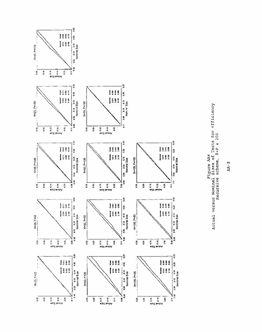
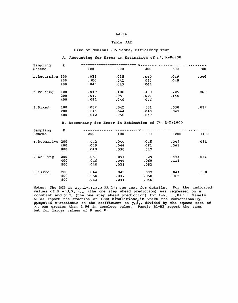
Table 4 has the results for the efficiency test. For the recursive and
fixed schemes, our procedure seems to be a little more accurately sized than it

19
was for mean prediction error. But for these two schemes the remarks made in
connection with Table 3 generally apply here as well.
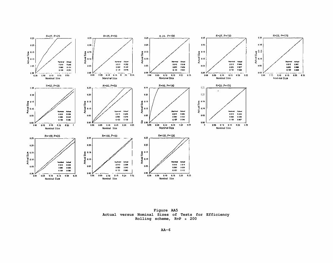
The rolling scheme, however, performs quite poorly for P/R>l. In fact,
for P/R>l, the over-rejection is so extreme that failure to adjust generally
improves the test statistic. For example, for P=50, R=25, panel A2 indicates
that our procedure had an actual size of 43%, while panel Bl indicates that use
of the usual least squares test statistic yielded a size of 7.2%.
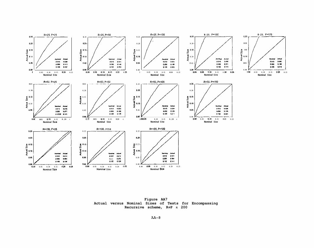
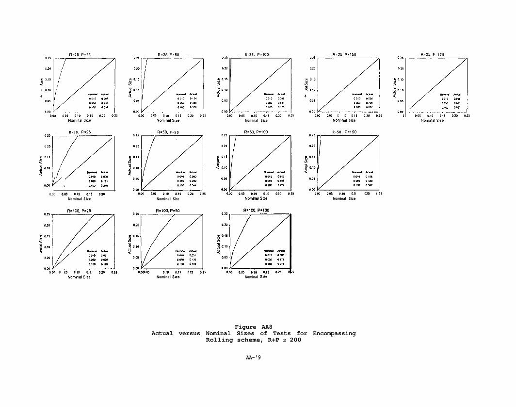
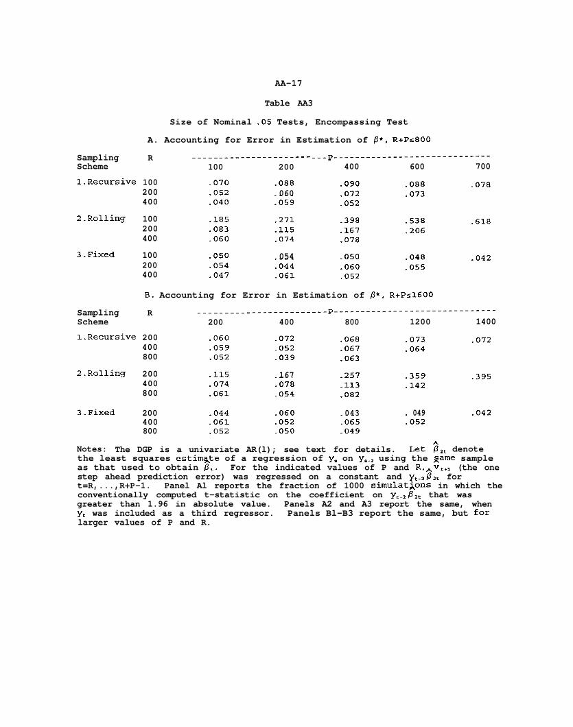
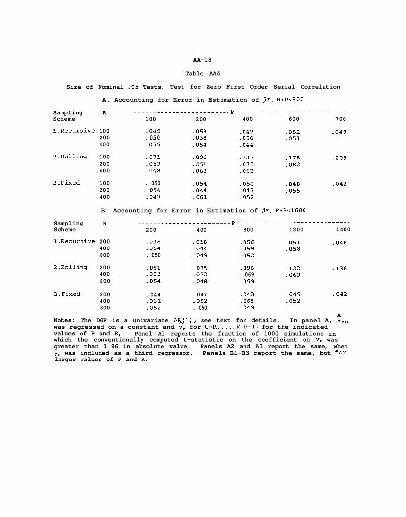
Tables 5 and 6 indicate that for the encompassing test and the test for
zero first order serial correlation, the Table 4 results apply qualitatitively:
For the recursive and the fixed schemes, our test statistics work adequately,
and dominate the unadjusted test statistic. But for the rolling scheme our
test statistic works poorly.
In Tables 4-6, the rolling scheme worked quite poorly for P/R>l. To see
how large a sample is required for tolerable accuracy of the asymptotic
approximation, we generated 1000 samples of size 1601; we report here certain
results with samples of size up to 1201 (full details are in the additional
appendix). We controlled the seed to the random number generator so that the
first 201 observations in each sample were the same as in Tables 3-6. We then
conducted the efficiency test for some larger sample sizes, holding P/R fixed
at 2 and at 4. The results are in Table 7. As may be seen, by the time the
sample size hits 1200, the result for P/R=2 is reasonably accurate (actual size
of .069), at least by the standards of Tables 3-6 and much other work on
hypothesis testing in time series models. For P/R = 4, however, substantial
mis-sizing still remains.
We conclude that our asymptotic approximation usually works reasonably
well, but that for the rolling sampling scheme relatively large sample size
sometimes are required.

2 0
Footnotes
1. We hope our work will be useful even for the interpretation of completed
papers. With the exception of one paper that came to our attention after this
paper was written (Hoffman and Pagan (1989) ), to our knowledge all such papers
have used standard regression statistics, without adjusting for dependence of
predictions on estimated parameters. We establish conditions for the
asymptotic validity of such statistics, and in some cases we are able to
propose adjustments for such dependence that can be made even without access to
the data. See sections 4, 5 and 7.
2. This test is most naturally run by regressing Y~+~- 2tYth
on yt- B t-lYt-1 -
Strictly speaking, our notation implies that Y~+~- 2 t-1Yt rather than Y~+~- Ztyt is
on the left: we assume that both left- and right-hand side variables are
constructed from the same estimate of p', and a rank condition presented below
rules out simply defining parameters so that the population parameter of
interest is 2x1 with a 2x1 period t estimate of ($,,z,.,)'. But this rank
condition is easily relaxed, and results may be generalized to allow the
natural version of this test. To economize on notation, we do not explicitly
do so in this paper.
3. See West (1996) and McCracken (1997) for further discussion of the
conditions under which F=O.
4. Note that this last condition rules out tests of nested (rather than
non-nested) models. Such tests are in Ashley et al. (1980) and Clark (1997).
An insightful referee has pointed out that some of our results do extend to
non-nested models; to conserve space, we do not consider such models here.
5. It is, however, possible to construct examples in which the results of
Theorem 7.1 fail. Let E, and u, be independent standard normals, v,=E$,,
x,=(Eq)+~, with Ex,#O, where all variables are scalars. Let a regression model
be yr=x&+v,, with estimation by OLS. Then S,,=Ev: (=EE:Eu:) , S,,=Ex,v:=Ex,Ev:,
S =Ex2v2hh t t, F=Ex,. This violates Theorem 7.1's assumption that there is a
constant term in the equation. Consider mean prediction error. Theorem 4.1
indicates that Pl/'$ E P-1'2C(yt+l-~t+l$t) is asymptotically normal with asymptotic
variance [Ev: - ~X,,E~,(EX:)-~EX,EV: + X,,(Ex,)'(E$v:) (EXE) -21 . This does not reduce
to AEv;&S,~ since Ex,#O and Egv: f ExzEv:.
Al
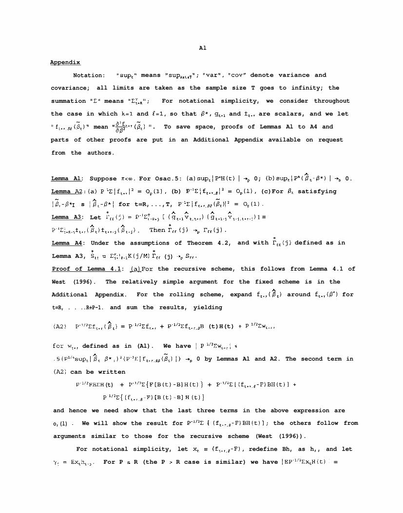
Appendix
Notation: 'lsupt" means ~~~~~~~~~~~~~ "var", "cov" denote variance and
covariance; all limits are taken as the sample size T goes to infinity; the
summation "E" means 1tCT=R8'; For notational simplicity, we consider throughout
the case in which k=l and f=l, so that P*, g,+, and ft+, are scalars, and we let
" f t*r,,w (it) I' mean 81$++T(FC) 'I. To save space, proofs of Lemmas Al to A4 and
parts of other proofs are put in an Additional Appendix available on request
from the authors.
Lemma Al: Suppose 71~03. For Osac.5: (a)sup,lPaH(t) 1 -Q 0; (b)sup,lP"(2,-fi*) 1 +p 0.
Lemma A2:(a) P-'L:{f,,,12 = O,(l), (b) P-1CIf,+,,B!2 = O,(l), (c)For p, satisfying
Iik* I s [2,-p*l for t=R,...,T, P-'EIf,+,,8B(&)- 12 = O,(l).
Lemma A3: Let F,,(j) E PmlE:=,+j [ ($,+~^Vt,t+~) ($t+l.jGt.j,t+r-j) 1 z
P~lZTt=n+,f,,, C$,) ft+r.j ($t.j) . Then F,, Cj) -y, r,,(j).
Lemma A4: Under the assumptions of Theorem 4.2, and with cLf(j) defined as in
Lemma A3, 6,, = C~:!,+,K(j/M) F,f (j) -+,p S,,.
Proof of Lemma 4.1: MFor the recursive scheme, this follows from Lemma 4.1 of
West (1996). The relatively simple argument for the fixed scheme is in the
Additional Appendix. For the rolling scheme, expand ft+,($t) around f,+,(p') for
t=R, . . ..R+P-1. and sum the results, yielding
(AZ) P-1'2Eft+r(;t) = P-1'2Ef,+, + P-1'2Ef,+,,,B (t)H(t) + Pm1'2Ewt+,r
for wthr defined as in (Al). We have I P-1'2Ew,+,i s
.5(P"4sUp,I~t-P*1)2(P~1~:fft+r,/ll(Pt) I) +p 0 by Lemmas Al and A2. The second term in
(A2) can be written
Pm1'2FBEH (t) + P-1'2E{F[B(t)-B]H(t)} + P-1'2E[(f,+,,,-F)BH(t)] +
P-1'2E{ (ft+r,8-F) [B (t) -Bl H (t) }
and hence we need show that the last three terms in the above expression are
o,(l) f We will show the result for P-1'2C [ (ft+r,8- F)BH(t)]; the others follow from
arguments similar to those for the recursive scheme (West (1996)).
For notational simplicity, let x, = (f,+,,B-F), redefine Bh, as h,, and let
yj = Ex,h,.,. For P L R (the P > R case is similar) we have [EP-"'Ex,H(t) i =
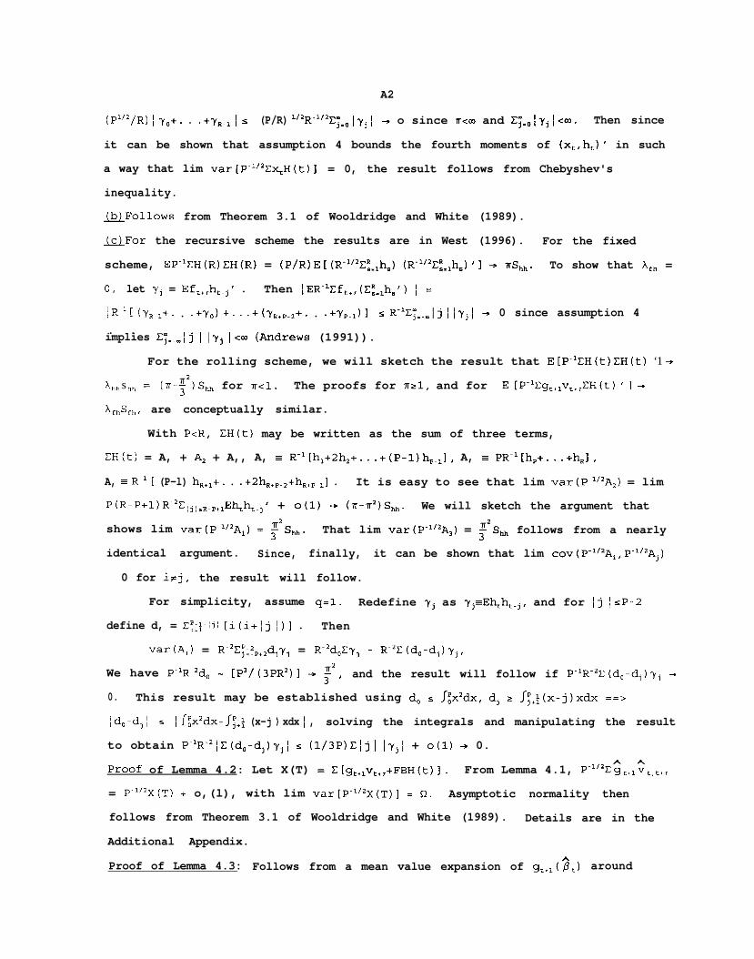
A2
(P"2/R) 1 yO+. . .+Y~.~ 1 s (P/R) 1'2R-1'2C;10 1 yj 1 + o since r<oo and Ey_,,I~~)cm. Then since
it can be shown that assumption 4 bounds the fourth moments of (x,,ht)' in such
a way that lim var[P- "2ExH(t)] = 0, the result follows from Chebyshev'st
inequality.
mFollows from Theorem 3.1 of Wooldridge and White (1989).
mFor the recursive scheme the results are in West (1996). For the fixed
scheme, EP-lEH(R)EH(R) = (P/R)E[(R-1/2Ei_,h,) (R-1/2E~Ilhs)f] + ?rS,,. To show that A,, =
0, let yj = Ef,+,h,.j' . Then iER-lCf,+,(Ez-,h,') [ =
/Rm'[ (yR.l+. . .+Y,,) +...+(Y~+~.~+. . .+')',.,)I 1 5 Rm'E;x.mlj 1 lyjl + 0 since assumption 4
. .implies Ei..-lj 1 Iyj i coo (Andrews (1991)).
For the rolling scheme, we will sketch the result that EIP-lCH(t)BH(t) ‘1 --)
A shh hh = (T-t")S,, for 7~~1. The proofs for 7~~1, and for E [P~'Eg,+,v,+,EH(t) ' ] --,
&lSfh I are conceptually similar.
With PcR, EH(t) may be written as the sum of three terms,
ZH(t) = A, + A2 + A,, A, = R-'[h,+2h,+...+(P-l)h,.,], A, = PR-'[h,+...+h,],
A, = R-l [ (P-l) h,+,+. . .+2h,+,.,+h,+,~,] . It is easy to see that lim var(P-1/2A2) = lim
P(R-P+1)R-2CIjirR.P+1Ehtht.j' + o(l) --, (r-r2)Shh. We will sketch the argument that
shows lim var(P-1'2A,) = T2S,. That lim var(P-1'2A,) = f2S, follows from a nearly
identical argument. Since, finally, it can be shown that lim COV(P-~'~A~,P-~'~PL~)
= 0 for i*j, the result will follow.
For simplicity, assume q=l. Redefine yj as yj=Eh,h,.j, and for lj IsP-2
define d, = cT;:mljl [i(i+[j [)] . Then
var(A,) = R-2Ey:?,+2djYj = Re2d,Eyj - R-'E(d,-dj)yj,
We have P-lR-"d, - [P3/(3PR2)] + f2, and the result will follow if Pm'Rm2E(do-d,)-yj +
0. This result may be established using d, L IEx2dx, dj t Iy;$(x-j)xdx ==>
jd,-d,; 5 1 J:x2dx-JT;: (x-j ) xdx 1 , solving the integrals and manipulating the result
to obtain P-1R-2[E(dO-dj)Yj[ 5 (1/3P)Clj/ lyjl + o(1) -+ 0.
PrOOf of Lemma 4.2: Let X(T) = E[g,+,v,+,+FBH(t)]. From Lemma 4.1, P-1'2CGt+lvt,t+rh
= P-1'2X(T) + o,(l), with lim var[P-"'X(T)] = R. Asymptotic normality then
follows from Theorem 3.1 of Wooldridge and White (1989). Details are in the
Additional Appendix.
Proof of Lemma 4.3: Follows from a mean value expansion of g,+,(2,) around
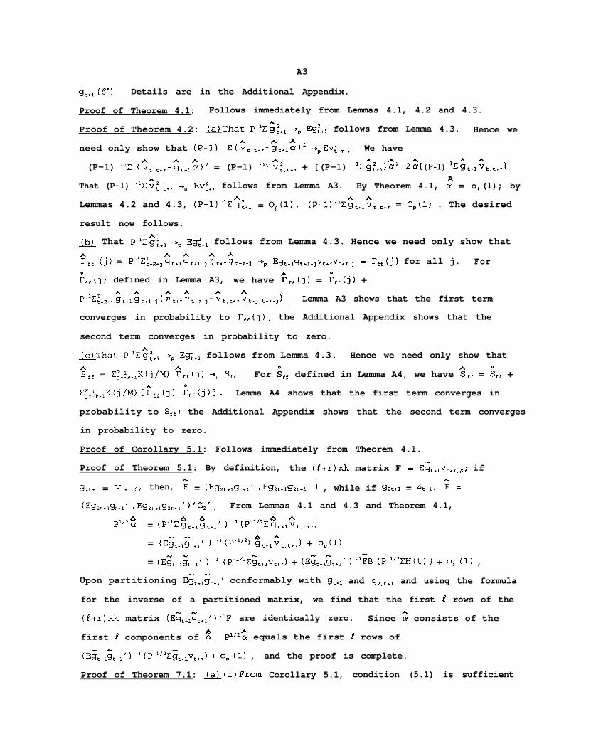
A3
g,+, (P') . Details are in the Additional Appendix.
Proof of Theorem 4.1: Follows immediately from Lemmas 4.1, 4.2 and 4.3.
Proof of Theorem 4.2: MThat P-'C$:+, -jp Eg:+, follows from Lemma 4.3. Hence weh A
need only show that (P-l)~1C(~,,,+,-g,+l~)2 jp Ev:+r . We have
(P-l) -'Z (;t,t+i-;trlG)2 = (P-l) -%&+, + [(P-l) -1$:+11 3 - 2.2 t (P-1) -lT;t+l~t,t+,l .
That (P-l) -iEG:,t+rA
-y, Ev:+, follows from Lemma A3. By Theorem 4.1, cy = o,(l); by
Lemmas 4.2 and 4.3, (P-l)-lC$:+, = O,(l), (P-l)-lZ$,+l$,,,,, = O,(l) . The desired
result now follows.
m That P-lE$:,l +p Eg:+, follows from Lemma 4.3. Hence we need only show that
cff (j) E P~'E~~~+j~t+l~t+l-j~t+r~t+r-j +p Egt+lgt+l-jVt*,Vt+,-j E F,,(j) for all j. For
i,,(j) defined in Lemma A3, we have G,,(j) = Fet(j) +
P-lx=t.R+jGC+lCt+l-j (~t+,~t+i-j-Gt,t+r~t-j,t+~-j) . Lemma A3 shows that the first term
converges in probability to l?,,(j); the Additional Appendix shows that the
second term converges in probability to zero.
@J-That P-'C$:+, +p Eg:+, follows from Lemma 4.3. Hence we need only show that
2 ff = XT:ip,lK(j/M) p,,(j) +p S,,. For g,, defined in Lemma A4, we have $,f = 8,, +
ET;i,+,K(j/M) [?,,(j)-;,,(j)]. Lemma A4 shows that the first term converges in
probability to Sff; the Additional Appendix shows that the second term converges
in probability to zero.
Proof of Corollary 5.1: Follows immediately from Theorem 4.1.
Proof of Theorem 5.1: By definition, the (4+r)xk matrix F E E&+l~,,,,B; if
g2,+1 = vt+,,ot then, F = (Eg,,+,g,+,' rEg2t+1g2t+l' 1 , while if g,,+, = Z,+l, FE
(Eg2tr1 t+1' fg E%t+,%t+,' ) 'G2' . From Lemmas 4.1 and 4.3 and Theorem 4.1,
pl/2~ = (P-l&+,&+,~ 1 -W~‘&+,~,,,+,)
= (E;;,,&+/ 1 -1(P-'12&,+l~,,,+,) + o,(l)
= (E;;,+,&+/ ) -' (P-1'2C&+l~t+r) + (E;;,,&+,' 1 -l:B (Pm"2ZH(t) ) + op (1) ,
Upon partitioning E&+lGt+lf conformably with g,+, and g,,,,, and using the formula
for the inverse of a partitioned matrix, we find that the first Q rows of the- ..s
(P+r)xk matrix (Eg,+lg,+l ')-lF are identically zero. Since G consists of the
first I components of g, P1/2$ equals the first ! rows of
(E&+1&+/ 1 -1(P-1'2Z&+lVt+,) + op (1) , and the proof is complete.
Proof of Theorem 7.1: M(i)From Corollary 5.1, condition (5.1) is sufficient
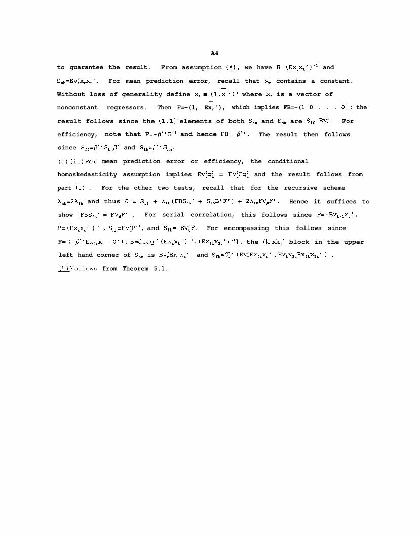
A4
to guarantee the result. From assumption (*I, we have B=(Ex&'Iml and
Shh=Ev:xtxt' . For mean prediction error, recall that x, contains a constant.- -
Without loss of generality define x,= (1,~~')' where xt is a vector of-
nonconstant regressors. Then F=-(1, Ex,'), which implies FB=-(1 0 . . . 0); the
result follows since the (1,l) elements of both S,, and S, are S,,=Ev:. For
efficiency, note that F=-p"B-' and hence FB=-P". The result then follows
since Sfr=P"S&' and S,,=p"Shh.
(a)(ii)For mean prediction error or efficiency, the conditional
homoskedasticity assumption implies Ev:g: = Ev:Eg: and the result follows from
part (i) . For the other two tests, recall that for the recursive scheme
h,=2& and thus R = S,, + h,,(FBS,,' + S,,B'F') + 2X,,F'VBF'. Hence it suffices to
show -FBS,,' = FV,F' . For serial correlation, this follows since F=-Ev~.~x~',
B=(Ex,x,' ) -', S,=EV:B-~, and S,,=-Ev:F. For encompassing this follows since
F= (-/~;'Ex~~x~',O‘), B=diag[ (Ex,x,')-', (Ex,,x,,' )-'I, the (k,xk,) block in the upper
left hand corner of S,, is Ev:Ex,x,', and Sfh=@;' (Ev~Ex,,x,' ,Ev,v,,Ex,,x,,' ) .
~Follows from Theorem 5.1.
AA-1
Regression Based Tests of Predictive Ability
Kenneth D. WestMichael W. McCracken
May, 1997Last revised January 1998
Additional Appendix
This not-for-publication additional appendix contains material omittedfrom the body of the paper to save space:
I. Additional simulation results:
A. Plots of Actual versus Nominal Sizes of Hypothesis Tests:Mean Prediction Error
RecursiveRollingFixed
EfficiencyRecursiveRollingFixed
EncompassingRecursiveRollingFixed
First Order Serial CorrelationRecursiveRollingFixed
B. Efficiency Test with large sample sizesRolling: P/R = 2Rolling: P/R = 4
C. Tables for large sample sizesMean Prediction Error
R+Ps800R+Ps1600
EfficiencyR+PZZ800R+Ps1600
EncompassingR+Ps800R+Pr1600
First Order Serial CorrelationR+Ps800R+Ps1600
II. Proofs:
Lemmas Al-A4Lemma 4.1 (for fixed scheme)Lemma 4.2 (additional detail)Lemma 4.3Theorem 4.2(b), (c) (additional detail)
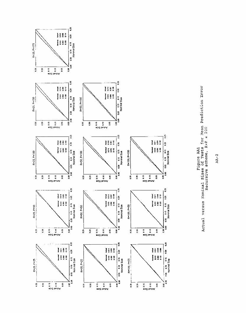
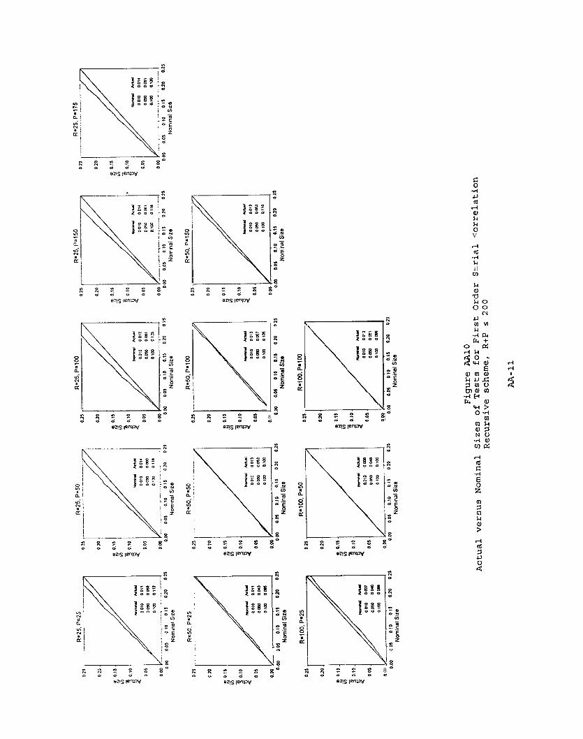
Figure AA1Figure AA2Figure AA3
Figure AA4Figure AA5Figure AA6
Figure AA7Figure AA8Figure AA9
Figure AA10Figure AA11Figure AA12
Figure AA13-aFigure AA13-b
Table AAl-ATable AAl-B
Table AA2-ATable AA2-B
Table AA3-ATable AA3-B
Table AA4-ATable AA4-B
a ggs0,;
5: i SEh
-7
5:2
I:: :: c 2 s 86 .5 d d d i
=!S v-w
::d
8a
‘-1.+ .B
cn
? .E
-;
xd
8d
:: 1 ” 0 s 8Od d d 0 d
%tIH! 80“,i
ffi “-
iIE “2
sl
iFI!Ii’JGE
i
%s0
L:: :: ” 5! s x00 a 0 d 0 0
ens IenPV
0 25R'25.P=25
0 25
0 20
8 085*3 OIO
20 05
owlt
0 25
0.20
Dii
0.0
2 0.10
?i!0.05
R=25. Pa500 25
0 20
(YY 0.15
129 O.lO
40.05
0.W(
!+25. P=lOO R=25.P=175
8 0.11
21010
Ii0 OJ
0.00 ..--~- ____-__.._ ___.(.___ -000 0.05 0.10 0.15 0.20 0.25
R=25.P=150
w O.”2 0.104
0 0,
0.000.04 0.05 0.10 0.11 020 02)
-1_WJa’l-i
f4cmn.l A.cNnOOfO OOYooy) OK5o.,m 0 111- ,._-
0.05 0.10 0.1J 020 0250.00 0 05 0.10 0 15 0.20 0Nominal Size
025
020
a 0.0.Yf23 0.10
2O.OJ
0.04
R=50, p-25
//
-w0 010 001200% o&Jo.,m o.,,,k
000 0.03 0.10 0.15 020 1Nominal Size
0.2,
0.20
& 0.15v)
il ;I:;
0.00
25
7
025
L
B 25
R=lW. P.25
/
-woom omoom ODUPm oooo
_- (_.__ -_,-_---<OW 0.20003 0 to 0.15
Nomml Site
0 20
8 PO*lo’,
0 05
OW
Nominal Site Nominal Size Nominal Size
R=50. P.150R.50. P=loO
0.04 0.05 0.10 0.0 020 tNominal Size
!+50. P=50
./”
-kwOOlO O.OIJ0.050 oca0 tm *.,,a
0.000.00 0.0, 0.10 0.0 0.20 I
Nominal Size
0.25 7
020
a
2
0.15
7 0.102l-7
w-
0DOlO 00,1
.OSom 00720.m 01u
77
Ii5 020 0.250.00 0.05 0.10 0.15Nominal Size
R=lOO.P*lOO
020
a 0.158
1 :I;;
R=lCG. P=50
01)0.05 0.10 0.15Nominal Size Nominal Ske
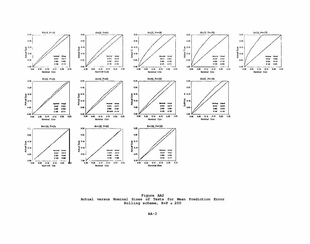
Figure AA2Actual versus Nominal Sizes of Tests for Mean Prediction Error
Rolling scheme, R+P I 200
AA-3
R=25. P=25
O W 0 05 0.10 0.1) 0.20 0.25Nominal Size
R=JO, P.257
8.25
-w
000 005 0.10 0.15 020 0Nominal Sire
R*lOO. P.25
Ncminal Size
0 25
0 20
a
iz
0.15
3 0.10
20 05
0.00t
R=25. P+50
L.- ̂ _,-_---- * --0 0.05 0.10 0.11 020 0.2J
Nominal Sire
R=SO. P=500.25 , /
0.20
0
B
0.15
0.10--
0 05 0010 aim
o,m 01330.04
0.04 0 05 0.10 0.1, 020 cNominal Size
R.100. P.50
0 05
0.040.00 0 05 o.,o 0.15 0.20 025
Nominal Size
R=25. P=lOO
8 0.11w'ij o.,o
20.05
0.00 IILO
0.25 1R=50. P=lO’l
0.20
0
i
0.15
1 0.102
L&f
-had0.05 0.010 om
0060 007sOKa 019
0.000.00 0.05 0.15 0200.10
R-100. P=lOO
0.05
0000.W 0.05 0.10 0.15 0.20 0.25
Nominal Size
R’25. P=150 R=25. P=175
0 0.05 0.10 O.!' 0.20 025Nominal Size
0.2)
0.20
R=50, P=lM
ms
0 . 0
f O.‘O
lo’l
-kw
0.05 0010 OOZJom eonotm Old
0000.00 0.05 0.10 0.15 0.20 025
Nominal Sits
m.Y
0.15(03 0.10
20 OJ
0.041
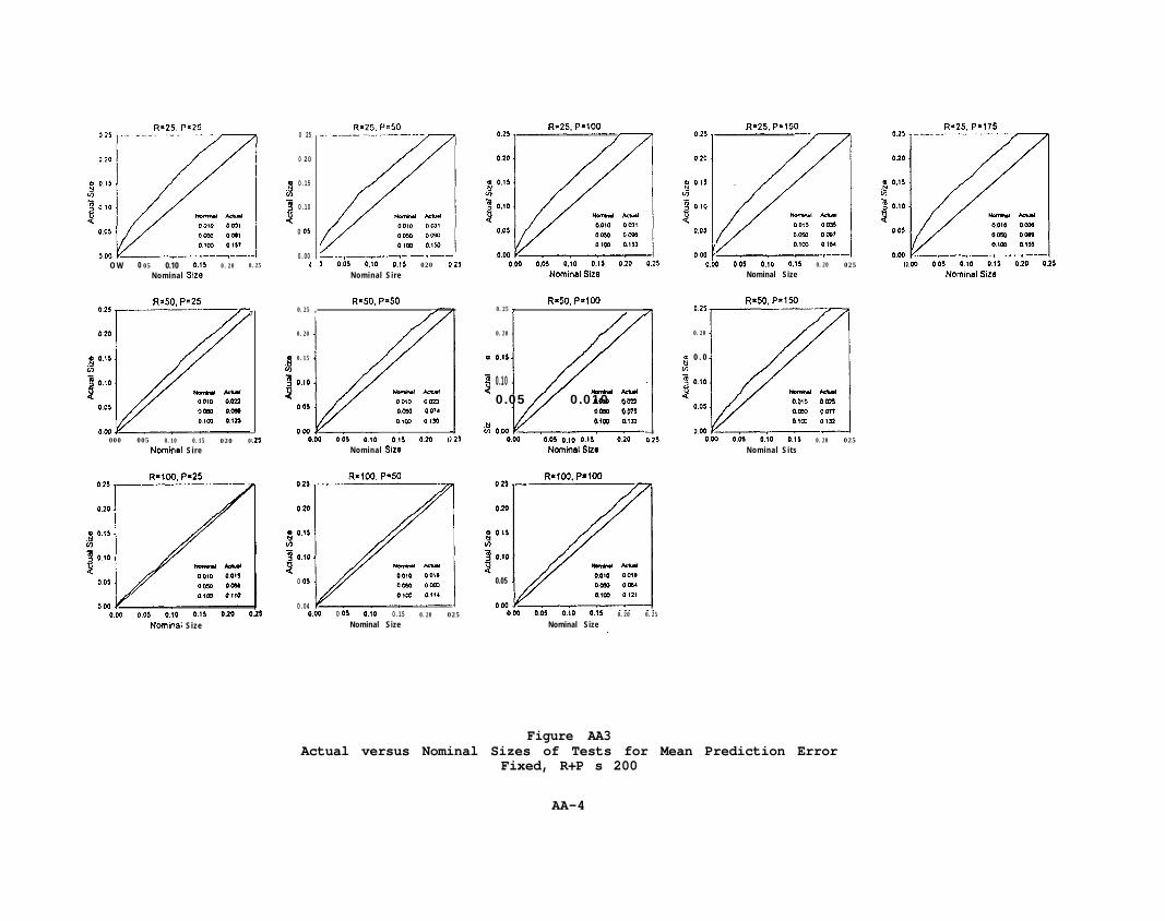
Figure AA3Actual versus Nominal Sizes of Tests for Mean Prediction Error
Fixed, R+P s 200
AA-4
E 2. “c I! 6 8 0D 0 0 0 0 d
=!S I=-mv
Z :: ” g 8 80 0 d 0 d d
n” .y ” z 80 0 d d dws 1mw
\I8:: :: r 2 s 8 00 0 0 d 0 0
ens I”W
?,0 .uU-J
a2-zd --
E8d
8d
x
2-Iiu-dwwW
Z :: ” 0 80 0 d d d dws (enw
:: 6 ” Z S 80
0 0 0 d d d
W 0, ” 5? 80 0 d d 0 d=!S WPV
8iA 8 Z t 8 8d d d d d d
=?s wwv
:: R ” 0 80 d d d 0 d
:: .?, ” 5! S 8 0d d d 0 d d
ens WPV
R=25. P=50 R - 2 5 . P=lOO
-.--.. ___,. -._, ( ---I000 0 05 o.to 015 0 20 0 25
Nomrd Size005 0.05 o.to 0.0 0 10 025
Nominal Size
R.25. P=lSO
; 1.1A
0 25R=25. P=175R=25. P=X
PI
ml Lchrl0010 ODD7ocm omOKM own
-.- ~._ -- _..,. --.. , -_ . .._.”
0 20
; 0.0v)7 P.IO23 O”O
I/k.+d k&al
0.05 OOlO ODMAM II-7
.I5V
““.-, “-,O!rn own0.0.3 -_- -.__, -.-0 00 0.05 0.10 O.!5 010 0
005
0.0-YOW 0 05 o.,o 015 b.20 0 25
Nominal SiteNominal SireNominal Sire
R’50. P=25-I_-------. _-.--0 25
0 20
0i
015
f O.'O0 05
0.04I..../lli/
-*Mooto 00xOKa 006o,m ocao
R.50. P.50 R=50. P=150R’50. PHOO0.25 ,-,- 0.25
0.20
g 015mf 0.103
0 05
0.000004 0.05 0 10 0.15 0.20 c
Nominal Size
77
325
0.200.20
008
8
0.150.15
33 0.100.10
A?A?
l!LLY/
-w-w
0.050.05 0.0100.010 octdoctdomom on2on2OX0OX0 02450245
0.00_..0.000.00 0.05 0.10 0.15 020 ,oi5 o.io o.is oio t
Nominal SizeNominal Size1.25 0.03 O.lO 0.15 0.20 (
Nominal Sire0.03 0.10 0.15 0.20 (
Nominal Size
R=lOO. P=50
020
,g o.t5In
3
0.10
Nominal Size
0.05
0.000.0-I 005 0 10 00 0 IO 025
R=lOO. P.25
0.00 005 010 0.15 020 0.25Nominal Size
0.25R=lOO. P=lOO
0.20
0 0.15ii
a
0.10
005
Nominal Size
- Andooto 0011om 0059o,m 0111
0.000.04 0.05 0.10 0.15 010 ( 5
Figure AA5Actual versus Nominal Sizes of Tests for Efficiency
Rolling scheme, R+P s 200
AA-6

R=25. P=250.25
020
& 0.,5
v)
2
2
0.10 I
005
000000
0 2 5
0 10
Q 0.15
v)
3
2
o.,o I
005
0.030.00
0.25R.25, P-100
0.20
0
iY
0.15
!I 0.10
0.05
0.00 ce,o(
025
0.20
,a 0.45
VI
4 0.10
I0.05
Nominal Size
R=50, Pa100
v
llarw hutOOlO OK40L-a omOlrn eon
0 .00 ---3 -.0.00 0.05 0.10 0.15 020 (
R=25. P - 1 5 0
OJ5 I
R=25, P.1750.25 ,
R=25, P.175A
0 10
,$ 0.15v)
-P
?I
o.,o-1 haal
005
0010 eonarm omlotm 0004
0c.l . , ,... . , __._,._0.00 0.05 0.10 0.,5 0.20 025
. , ,... . , __._,._0.00 0.05 0.10 0.,5 0.20 025
Nominal SizeNominal Size
R=25, P=50
0.20
m.2 0.0
3 0.10
9
v
Wrul #.%a,0.05 oom 0021
occ.3 0055Olrn 0001
0.w -.--_- -.. -,._.000 0.05 0.10 0.0 0 20 0 25
Nomml SLZ.S
R’50. P=25. ._ ..-
A
-kw0010 00soaa OMOlrn om3
__ _, __. , . _. . .._ _ _, - .I.250.00 0.05 0.10 00 0.20 t
Nominal Sirs
Nomml Size
R=50. P’50_ ---. .--_..- ..___
Nominal Size
R=50. P=1500 15
0.10
8 0.15
u)
f
4
0.10 I
0 05
0.00 -0.00
0 25
0 20
8 015
m
$ 0.10
20.05
0.04
//
;25
,
3 25
ail/
NaM.kbl0010 OOQamc 00som 0 070 /I:/
--oom omrODyl 0051OIrn 0014
_. (___ , _-. , - . . . . . --0.05 0.10 0.,5 020 1
:.-.,, -.-0.M 0.10 0.15 0 20 5
Nominal Size Nominal SiraNominal Size
R.100, P=lOO
wkwO.OIO om70.00 0041
0.00 0.1 0.10 0.15 020 0Nominal Sirs
R=100, P=500.25
0.20
0ii 0.0
f O.‘O0.05
004m
-Acwomo 00xocm 0041Olrn 0001
R=lOO, P.25015 ,-
000 0 05 0.10 0.15 020 0.25 0.04 0 05 O.,O 0.15 0.29 0 25Nominal SizeNominal Size
Figure AA6Actual versus Nominal Sizes of Tests for Efficiency
Fixed, R+P s 200
AA-7
Q O.l5
i
0 10
005
0.00 I0 0.05 0.10 0.15 0.20 0.15
Nominal Site
R’50. P.25 R=50. P=50 R.50, P=loO025
0 PO
0 015
::
0.10
003
/
-_.-_._-.-.-. _ ..--
P&aldmlwoom 001500 0 on0 'co 0.1‘1
R=25. P=25 R=25. P=50 R=25. P=loO0.25 0.25
0.20
& 0.15
i:::
v
!sudrd*c(uloom om,Op50 O’SOlrn ox),
OOC 005 0.10 0.15 0.20 t
Nominal Size
R.100. P=25
000 0.05 0.10 0.15 020 0.25Nominal She
025
0.20
g 0.15
In
?f 0.10
0.05
0.W kII.00
020
ob5 o.io o.i5 oio 0 I5Nominal Sue
Homn*ee.d0010 eon0050 Olrn
005 0.10 0.15 020 cNominal Size
0.25R=lCO. P f 5 0
-AN
0.05OOID 0011boy) 0070
0.00000 0.05 0.10 0.15 0.20 C
Nominel Sire
0.001
0.25
0 20
,z 0.15
'0
0.05
0.W,
0.05 0.10 0.15 020 0.25Nominal Size
o.b5 0.10 0.15 0.20 c 004 0.05 b.,O 0.15 020 0.25Nominal Site Nominal Size
R=lOO. P.1000.25
0.20
,%j 0.15u)
0.10
0.05
1";
0010 0011p.mO OMom 0.14,
0.000.00 0.05 0.10 0.15 0.20 0.25
Nominal Slzo
- karl
R - 2 5 . P=150
0.20
m
20.15
0.10
0.05
0.090.00 0.05 0.10 0.15 0 10 0.15
020
0 00
i
1 O.'O005
0.00
0 *5
0.20
?i O.'Im
t:
0.00
R=50. Pm150-:
I67
-wOOlO omcODxl 01som 0221
Nominal Sire
R - 2 5 . Pa175-//‘I
0 05 0.10 0.15 010 0.25Nominal Size
Figure AA7Actual versus Nominal Sizes of Tests for Encompassing
Recursive scheme, R+P s 200
AA-El
0 2,
020
8 00u)
3 0 10
40 0,
I
000 /0m
R=25. Pa25
Nominal SIZO
R - 5 0 . P=25
0 200 00
t -ku010 I77
0 21
o.wv. Olrn 024
0.00 0.05 0.10 0.1s 020 INominal Size
R=l&l. Po25
ow 0 01 010 0.1, 020 0.21Nomtnal Stze
R=25. P=50
I I --I000 0 05 0 10 0 I5 020 021
Nomml Sm
R=SO. P - 5 0
020
& 0.1su)-
0.10-1 w
0.05
000 --0.00 0.0) 0.10 0.11 0.20 0.21
Nominal She
02S
0.20
8 0.0
1 0.10
0.05
1000 -004
R=lOO. P=50~--
k”;
-kw0010 OrnlODYJ OI22O!rn otoo
ob5 o.;o oh 020 tNominal Sue
R - 2 5 . P=lM)
0.21
0.20
,g 0.15v)-! 0.10
0.05
0.00
R--50. P=lM)
-kMo.o,o 0 !&.Iowl ow0.m 0411
0.00 0.03 o.to 0 . 0 020 cNminel Site
0.00 001 O.lO 0.15 0.20Nominal Size
-wPO,0 omom 0171arm 0111
0.W 0.05 0.10 0.11 0.20 cNominal Size
R=25, P=150
Nomml Size
0.20
8 0 0v)
3 0 10
40 05
000 .____,___,_ -__ . . . . . - __...0.00 0.05 0 (0 011 0.20 0.2)
0 21
0 20
,$ 01,v?
3 0.10
20 01
0040
R - 5 0 . P=150
010
8 o.,,v)
3 0.102 -w
0.0,0010 0,sOKa 0.54om OYl
0040.00 0.05 o.to 0.0 020 t
Nominal Size
R=25. P - 1 7 5
77
Nominal Sm
Nonlrul ha”,0010 om00s OM!o,m on7
. , ,. _ -. .-_.-0 05 0.10 0.15 0.20 0.25
Figure AA8Actual versus Nominal Sizes of Tests for Encompassing
Rolling scheme, R+P b 200
AA-‘9

0 25
0 20
& OI,
*
3 0 10
0 0,
0.00
R=25. P=25___.. ._ -.--.- ..-.- - - 02,
020
2 0.11IA4 0.10
40.05
0.00t
0.25
0.20
0 0.0i?
!I
0.10
0.w
000t
R=25. P=500 25
020
8 0.13
tlg 0.10
90.05
004
R=25. P=150 R=ZS. Pa175-A- --__
/
tame-4 hsalomo om,0011) oweOK0 om-.-
000 0 0, 0.10 0.0 0.20 0.25
.=25. P=100
/I
-.--. _--___-
A
rlc.Nr.1 he4
ooto om
080 omd
o,m DOD7
0.20
jo.,o. /
8 0.1s.In
- MI!
4 0.05 1 / ;g “,z /ooov. . 0.m ---I 0 m
0.00 0.05 O.IO 0.15 0.20 0.2,Nominal Site
_r--.--.--I0.01 0.10 0.1, 0 20 a.23 0.04 0.0, 0.10 0.11 0.20 0.25
Nomlnsl Sire Nominal SireNominal SIZS
R=SO. P-400.2!
0 20
0II
o.,,
-4 010
0 05
OC4
Nomml Slza
R.50. P.25_------.-_-.
I- - c m - - - - - -
0.W 005 O.fO 0.0 020 INominal Sirs
R=50. Pal 00 R - S O . P=150
0.03 0.10 0.15 020 0Nominal Size
0.25
0.20
0.Y 0.15*
j 0.10
40.0,
0.00,
0.25
0.20
B 0.023 0.10
20.05
0.W/
--omo 0.m00% omatm Olrn
-0.0, o.to 0.15 0.20 0 21 0.W 0.05 0.10 0.t5 0.20 0.25
Nominsl Size Nomlnsl Size
R.100, P=500.25
0.20
0D
O.,I
iI
0.10
m
-MH
0 05DO,0 0010^-^ as..
VVW YMotm omam
R=lW. Pa25
000004 0 03 0.10 0.15 010 0.26
Nominal Site
R=lW, P=lW
_.--0.M o.io
4OC-3 0.15 0.20 011
Nominal Site0.00 0.1 0.10 0.15 010 0.25
Nominal Size
Figure AA9Actual versus Nominal Sizes of Tests for Encompassing
Fixed, R+P z 200
AA-10
L;e R ” 5 8 8d 6 d 0 d8
d
::ci
R0
z6 3u)
?E
2sd
8d
:: R II 0 s 8d
0 0 0 d 0 d
s
:: R 'II 2 Is 8d d d d d 0
dztiV
e-4ld-4kalrn
0 25
0 10
& 00v)I 0 ,o
0 05
0000
0 25
020
0iz
015
1;;;
c-000
030
e 0.0.cIv)
0.40i ,
025 -
v
-M3
005Oblb DotIomo Poyom 0115
ow -- ~.-- .__. ---.. _._-000 0 05 0 IO 0.15 0 2 0
R-25. P=25
Nom~nel SIZO Nommal Size
R=50. P=25 R550, P=50_ ..-_ .._ _ __..___ -
p=/
-ku0 010 001,omo oomarm 0.055
0 05 0.10 0.15 020 0Nominal Sirs
R*lOO. P=25
Nominal Size
000 005 0 lo O.I5 0.70 0 25
0 25020
P)s: 0.15
1
y;
10.00 -0.00
--____
6’
-Lcwoe,o 00x*cm ocma m 0 m
o.bs 0,io o.i5 0.h 0Nominal Size
hi5
FWOO. P=50
ow 0 05 0 (0 0.15 010 0Nomnal Size
R=25. P=lOO
-._-0.w 0.05 0.10 0.15 020 0 25
Nominal Slte
R=50. P=lOO
::I I//
0 0.15
i5f
//HarwLcu
0.03
I//
0010 0045o.oyI 010Olrn on4
0.20
,$ 0.,5In
30 10
0.25R=100. P=lOO
v
-Mul
0.05 0010 oota0050 0 onom 0 0,
PO00.04 0.05 0.10 0.15 0.20 <
Nominal Size
0.05 0.10 0.15 0.20 c 0.00 0.05 0.10 0.15 0.20 0:Nomlnal Size Nominal SLe
I5
R=25, Pa150
- . _-_-boo Il.05 0.10 0.15 020 0.25
Nominal SIZO
0.20
R=50. P.150
025R=25. P.175
0 IO
3 0.15G
2
2
010 I - I ; ’
- h%nl
0 05 oow 01uomo om3cm on,
0.00 --,-. ,____ --_--0.00 0.01 0 10 0.15 0.20 0.25
Nomml Size
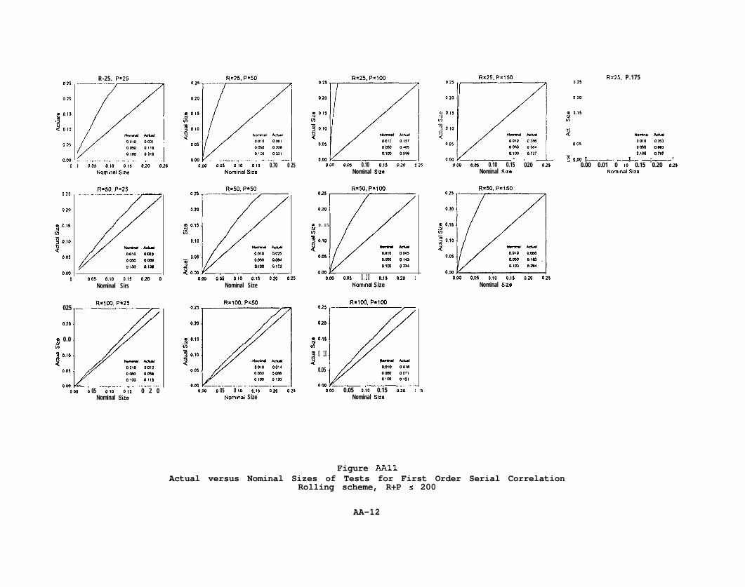
Figure AA11Actual versus Nominal Sizes of Tests for First Order Serial Correlation
Rolling scheme, R+P s 200
AA-12
R=25, P-25_----__--R=25. P=50 R=25. P=lOO R=25. P=150
0.25R=25. P.175_______~
-1 kt.40 0 1 0 bblbOmO OOCQOIO, OW1
0.25
0.20
ai
0.15
3 O.,O
40 05
0.00I
0.25
0 20
as
0.15
-j 0.10
$0.05
0.W L-------,-----000 0 05 0.10 0.15 020 0
Nominal Size
0.20
01 0.151
-j O.!b
20 05
000,
025
0 20
0 IO
0 05
0.W
0 25
0 20
& 0.15v)2 0,O
30 01
0 000
Y 0 25
0 20
Nrnd AMIOOlb 00X0060 ow4Olm Oop1
0 015
s12 010
20 05
N0ne.d LcMlOOIO omooc?a eta
0 05 0.10 0 !5 0 2 0Oil000
,Nommal Sue
0.05 0.10 0.0 0 20 025Nominal Stze
R=50. P=25 R.50. P=500 25
010
OW0.r 005 0.10 0::” 0: 025-.-__-- ._____ -.-._,- --.
Nominal Sire
000 v------,~I0.00 005 O.,O 0.,5 0 20 0.25
/
nmi..ll h3.n0010 ocmemo owom 0103
_,__,_____._~
0 . 0 5 0.10 0.15 020 <Nominal Sire
I,w
I, -
R=50. P=150
- -OOlO 0010ODY) 001,Oxu O!rn
0.05 0.10 0.15 0 20 0 25Nominal Size
R.50. P=loO-015 _-
0 20
8 0.15m
3 0.10
20.05
0.00 . 1 I0.00 0.05 0.10 0.15 0.20 0.25
Nominal Size
015 T-
020.
g 0.15v)
3 010
$0 05
0.00 005 O.,b 015 020 0.25Nominal SizeNomnal Sue
R*lW. Pa25 R=lCG. P.50 R=lOO, P=lCQ025 1-
090
0 0.15
i
I*.'*
0.05
-MulOblb 00100050 004OK0 OM
0.00 L004 0 05 0.10 0.15 0 20
Nominal Siza
0 25
010
j 015
m
3 0.10
2
0.05
0.25
020
- -0010 OmPm0 0040OX., OlW
9) 0 . 0iz
1 0.10
$003 O(IyI 0068
DC0 ODgl
0.05 b!O 015 0.X t OW 0 05 O.,O 015 0 20
Nominal Size Nominal Size
1‘50.25
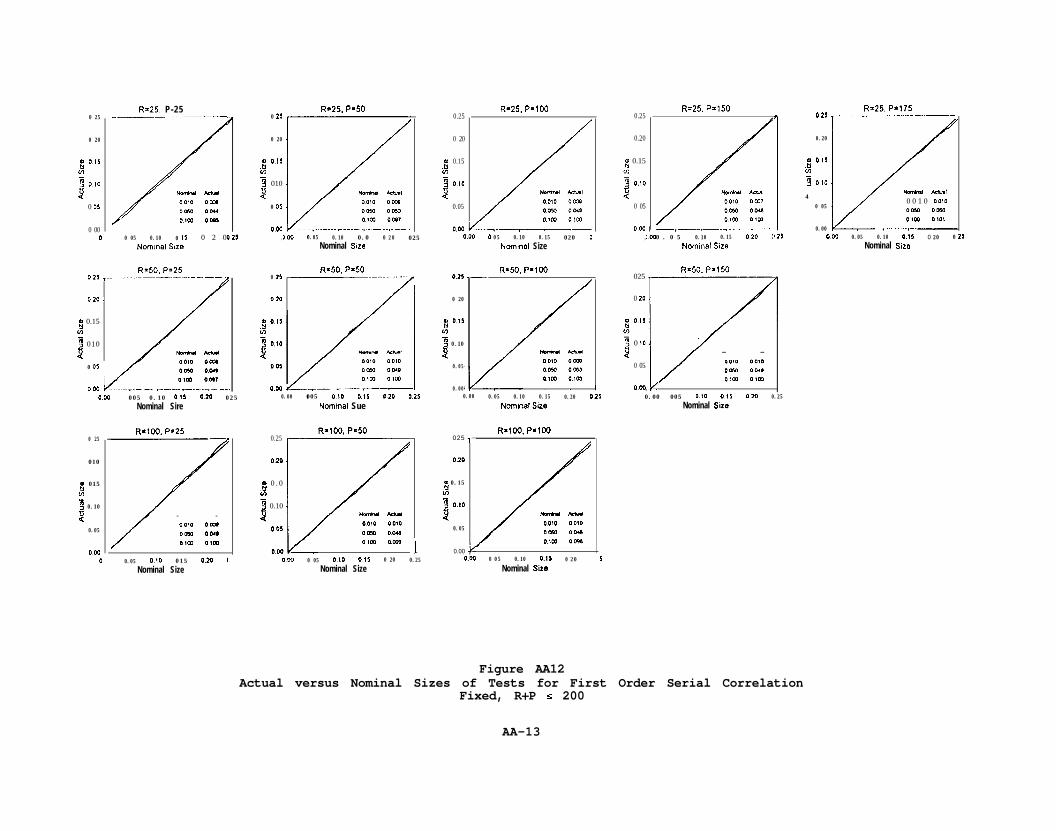
Figure AA12Actual versus Nominal Sizes of Tests for First Order Serial Correlation
Fixed, R+P s 200
AA-13

1.0
0.9
0.8
0.7
0.6
Ez 0.5z2 0.46
0.3
0.2
0.1
0.00.0
Rolling, P/R = 2
0.2 0.4 0.6Nominal Size
0.8 1.0
1.0
0.9
0.8
0.7
0.6
8z 0.5i5s 0.46
0.3
0.2
0.1
0.0
I
i’-_
Rolling, P/R = 4
I I I I
0.0 0.2 0.4 0.6
Nominal Size0.8 1.0
Figure AA13-a Figure A.A13-b
Actual versus Nominal Sizes of Tests of Efficiency Actual versus Nominal Sizes of Tests of Efficiency
Rolling scheme Rolling Scheme
P/R = 50/25, loo/SO, 200/100, 400/200, 800/400P/R = 100/25, 400/100, 800/200
AA-14
AA-15
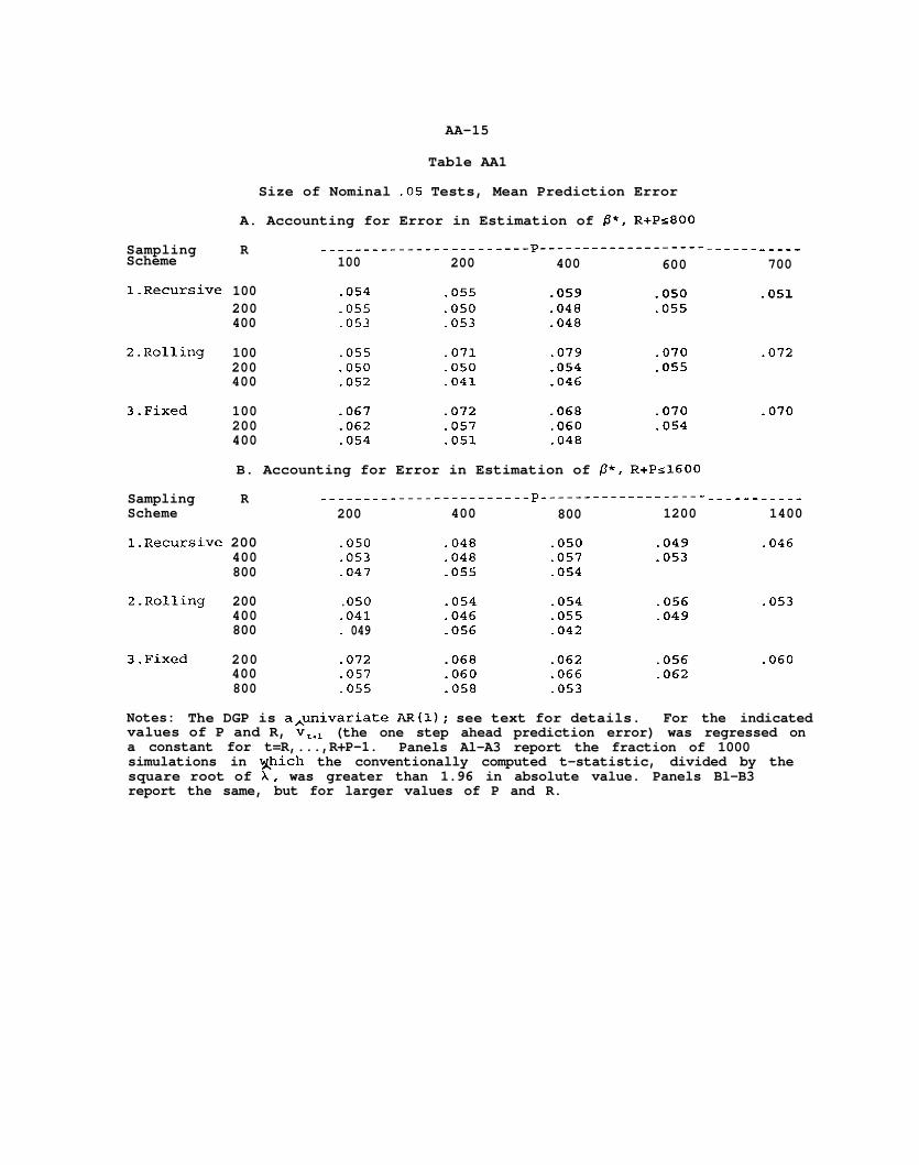
Table AA1
Size of Nominal -05 Tests, Mean Prediction Error
A. Accounting for Error in Estimation of o*, R+Ps800
Sampling R ------------------------p---------------------Scheme 100 200 400 600
l-Recursive 100 -054 -055 .059 -050
2.Rolling
3.Fixed
200 .055 -050 -048 -055400 .053 -053 -048
100 .055 -071 .079 .070200 -050 .050 -054 -055400 -052 .041 -046
100 .067 -072 .068 -070200 -062 -057 -060 .054400 .054 -051 -048
B. Accounting for Error in Estimation of P*, R+Ps1600
Sampling R ------------------------p---------------------Scheme 200 400 800 1200
l-Recursive 200 -050 -048 .050 -049400 .053 -048 .057 -053800 -047 -055 -054
2.Rolling 200 . OS0 .054 -054 -056400 .041 .046 -055 -049800 * 049 -056 -042
3.Fixed 200 -072 -068 .062 -056400 -057 -060 .066 -062800 .055 -058 -053
------
------
-----700
-051
.072
-070
_----1400
.046
.053
-060
Notes: The DGP is a&r&variate AR(l); see text for details. For the indicatedvalues of P and R, v,,, (the one step ahead prediction error) was regressed ona constant for t=R,...,R+P-1. Panels Al-A3 report the fraction of 1000simulations in xhich the conventionally computed t-statistic, divided by thesquare root of X, was greater than 1.96 in absolute value. Panels Bl-B3report the same, but for larger values of P and R.
AA-16
Table AA2
Size of Nominal -05 Tests, Efficiency Test
A. Accounting for Error in Estimation of p*, R+Ps800
Sampling R ------------------------- p---------------------.Scheme 100 200 400 600
l-Recursive 100 -039 -035 -040 .049200 _ 050 042 040 .045400 -040 :049 :044
2.Rolling 100 -049 -108 -409 -705200 .042 051 -091 -145400 .051 :046 .046
3.Fixed 100 -032 042 031 -038200 045 :044 :043 .041400 :042 .050 -047
B. Accounting for Error in Estimation of @*, R+Pr1600
Sampling R ------------------------p------------------------Scheme 200 400 800 1200
l.Recursive 200 .042 -040 .045 -047400 -049 -044 -061 -061800 -048 -038 -047
Z-Rolling 200 -051 091 .229 -424400 -046 :046 069800 -048 -038 :os3
-111
3.Fixed 200 -044 .043 .037 .041400 .oso .047 .058 _ 079800 -053 -041 .046
-_. - - - - - -700
-046
.869
-037
__------1400
.051
.566
.038
Notes: The DGP is a,univariate AR(l); see text for details. For the indicatedvalues of P and,R, vCel (the one step ahead prediction) was regressed on aconstant and y,Pt (the one step ahead prediction) for t=R,...,R+P-1. PanelsAl-A3 report the fraction of 1000 simulations,in which the conventionallysomputed t-statistic on the coefficient on y,@,, divided by the square root ofX, was greater than 1.96 in absolute value. Panels Bl-B3 report the same,but for larger values of P and R.
AA-17
Table AA3
Size of Nominal .OS Tests, Encompassing Test
A. Accounting for Error in Estimation of P*, R+Ps800
Sampling R ___________--_____-___ ---p-----------------------------Scheme 100 200 400 600 700
l-Recursive 100 -070 -088 .090 .088 .078200 -052 060 .072 .073400 -040 :oss -052
2.Rolling 100 -185 -271 -398 -538 -618200 -083 -115 -167 -206400 -060 -074 -078
3.Fixed 100 .050 054 -050 -048 .042200 .054 :044 .060 -055400 -047 -061 -052
B. Accounting for Error in Estimation of p*, R+Ps1600
Sampling R ------------------------p--------------------------------Scheme 200 400 800 1200 1400
l-Recursive 200 -060 -072 .068 -073 -072400 -059 -052 .067 .064800 -052 -039 .063
2.Rolling 200 .115 167 -257 -359 -395400 .074 :078 -113 -142800 -061 -054 -082
3.Fixed 200 -044 .060 043 _ 049 -042400 -061 -052 :065 -052800 -052 -050 -049
Notes: The DGP is a univariate AR(l); see text for details. Let ii,, denotethe least squares estimate of a regression of y. on yed2 using the game sampleas that used to obtain 0,. For the indicated values of P and R,Avv,,I (the onestep ahead prediction error) was regressed on a constant and yte2Pzt fort=R,...,R+P-1. Panel Al reports the fraction of 1000 simulat&ons in which theconventionally computed t-statistic on the coefficient on yCW2Pzt that wasgreater than 1.96 in absolute value. Panels A2 and A3 report the same, whenyr was included as a third regressor. Panels Bl-B3 report the same, but forlarger values of P and R.
AA-18
Table AA4
Size of Nominal .05 Tests, Test for Zero First Order Serial Correlation
A. Accounting for Error in Estimation of P*, R+Pr800
Sampling R -------------------------p-------------------------------Scheme 100 200 400 600 700
l-Recursive 100 -049 .053 .047 .052 -049200 050 -038 .056 -051400 :055 .054 -044
2.Rolling 100 -071 -096 .137 -178 -209200 -059 051 .075 -082400 -048 :063 -052
3.Fixed 100 _ 050 .054 -050 -048200 054 -044 -047 .055400 :047 -061 -052
-042
B. Accounting for Error in Estimation of P*, R+Ps1600
Sampling R ------------------------p--------------------------------Scheme 200 400 800 1200 1400
l-Recursive 200 -038 .056 .056 .051 -048400 -054 -044 -059 -058800 _ 050 -049 -052
2.Rolling 200 051:063
075:052
.096 -122 -136400 _ 069 -069800 .054 .048 -059
3.Fixed 200 ,044 047 -043 -049 .042400 -061 :052 065
:049-052
800 -052 - 050A
Notes: The DGP is a univariate q(l); see text for details. In panel A, v.,,was regressed on a constant and v, for t=R,...,R+P-1, for the indicatedvalues of P and R,. Panel Al reports the fraction of 1000 simulations inwhich the conventionally computed t-statistic on the coefficient on v, wasgreater than 1.96 in absolute value. Panels A2 and A3 report the same, whenyt was included as a third regressor. Panels Bl-B3 report the same, but forlarger values of P and R.
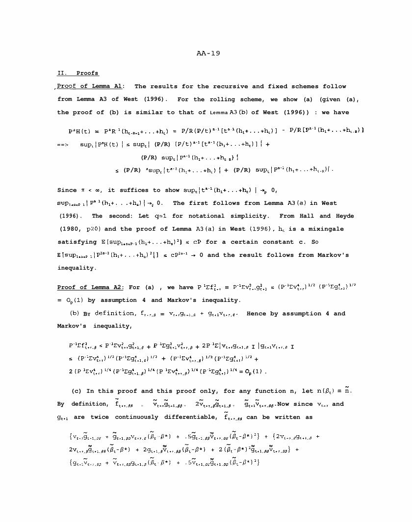
m-19
II. Proofs
,Proof of Lemma Al: The results for the recursive and fixed schemes follow
from Lemma A3 of West (1996). For the rolling scheme, we show (a) (given (a),
the proof of (b) is similar to that of Lemma A3(b) of West (1996)) : we have
PaH(t) 5 P"R-l(ht-R+l+...+h,) = P/R(P/t)=-'It"-'(h,+...+h,)] - P/RIPa-'(hl+-..+ht-~)]
==> sup,;P=H(t) 1 < sup,: (P/R) (P/t)=-'[t"-'(hl+...+h,)] 1 +
(P/R) suptIP=-'(hl+...+ht.J [
s (P/R) =~up~~t-~(h~+...+h~) 1 + (P/R) s~p~~p~-~(h~+-. -+&-,I i.
Since 51 < 03, it suffices to show supt[ta-l(hl+...+h,) 1 +p 0,
suplrsrP.lj Pa-'(hl+. . .+h,) ; jp 0. The first follows from Lemma A3(a) in West
(1996). The second: Let q=l for notational simplicity. From Hall and Heyde
(1980, ~20) and the proof of Lemma A3(a) in West (1996), h, is a mixingale
satisfying E[~up~~~+~(h~+...+h~)~] s CP for a certain constant c. SO
E tsuplrSrPml; P2a-2 (h,+. . .+h,) 2 i I s cPZael + 0 and the result follows from Markov's
inequality.
Proof of Lemma A2: For (a) , we have P-'If:+, E P-lCv:,,g:+, s (Pm1C~:+,)1'2 (P-1Cgz+l)1'2
= O,(l) by assumption 4 and Markov's inequality.
(b) BY definition, ft+r,b = vt+rgt+l.B f gt+lvt+r,8- Hence by assumption 4 and
Markov's inequality,
P-lCf2t+r,fl 5 p-l~v:+,g:+l,, + p-'n3z,+lv:+,,, + 2P1Z Ivt+r%*1.B I Igt+lvt+,,LT I
s (P-=cv:+,)1'2(P-'cg4 t+1.a )li2 + (P-?Yv4t+r,8) 1'2 (P-leg:,,) 1'2 +
2 (P-lEv;+,) II4 (P‘lcg:+l,,) lf4 (P-?Ev;+,,8)1/4 (P-?Eg:+l)'/4 = O,(l) .
(c) In this proof and this proof only, for any function n, let n(&) = G.
By definition, Etr.88 = K+&+l,B8 + G+,,&+1,B + ~t+l~t+,,BB- Now since vt+, and
g,,, are twice continuously differentiable, ft+,.&7 can be written as
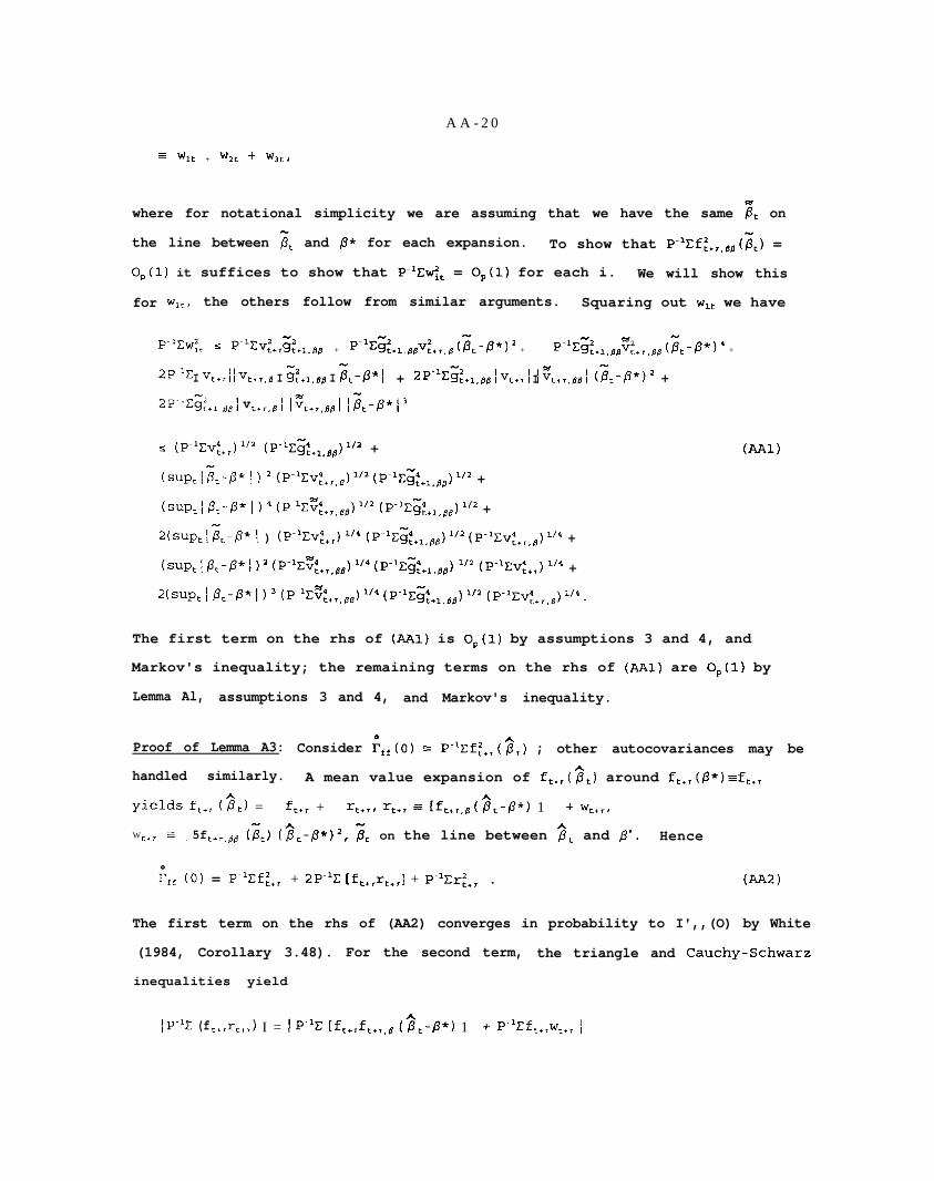
A A - 2 0
= W1t + W2t + W3t,
where for notational simplicity we are assuming that we have the same F, on
the line between ,& and /3* for each expansion. To show that P-lXf:+,,BB(zt) =
O,(l) it suffices to show that P-'Cw& = O,(l) for each i. We will show this
for wltr the others follow from similar arguments. Squaring out wit we have
P-lrw;t S P-'/3? -2t+r%+l.BB + p-la ,&J:+,,fi G,-P*) 2 + p-‘Eg:.,,,,~:+,.,,(il,-P*) 4 +
2p-‘E I vt+r I IV,+,,@ I g:,,,,, I L-P* I + 2-g:+,,,,1 Vt+rl I' '%,,,J G,-P*P +
2P~'cg:+, 88; vttr.ol I~t+r,~.BI li3,-P*I'
I; (P-Tv4,+,)1'2 (P-lCa+l,BB)l'a +
(SUP,&-P* I) 2 (P-1~v:+,,B)1'2(P-1c;;:+1,BB)1'2 +
(sup,; 6,-P* I ) 4 wC~t+r,BB)1'2 (P-1z~t+l,$J1'2 +
2 (suP,l;,-P* I ) (P-lm;+,) 1'4 (P-1c~t+1,BB)1'2(P-1cv:+,,8)1'4 +
(sup,lP,-p* 1 I2 (P-1~~:+r,88)1'4(P-1C~t+l,&qJ 1'2 (P-lcv:,,) 1'4 +
2 (sup, I B,-P* 1) 3 G-L~7t+,,88)1'4 (P-1r;;4t+l,BB)1'2 (P-1cv~+,,,J1'4.
(Z-1)
The first term on the rhs of (AAl) is O,(l) by assumptions 3 and 4, and
Markov's inequality; the remaining terms on the rhs of (AAl) are O,(l) by
Lemma Al, assumptions 3 and 4, and Markov's inequality.
Proof of Lemma A3: Consider i,,(O) = Pm'Ef:+,($,) ; other autocovariances may be
handled similarly. A mean value expansion of ft+,($t) around ft+,(P*)=ft,,
yields ft+, (2,) = f,+, + rt+,, q+, = [ft+,,e(??t-P*) 1 + wt+,,
Wt+r = . 5ft+r,B8 Gd (zt-P*)2, ;t on the line between 3, and 0'. Hence
f-f, (0) = P-Yf:,, + 2Pm1C [ft+,rt+,l + P-'Er:,, . (AA2)
The first term on the rhs of (AA2) converges in probability to I',,(O) by White
(1984, Corollary 3.48). For the second term, the triangle and Cauchy-Schwarz
inequalities yield
1 p-1.Z (f t+rrt+r ) I = I p-‘c rft+,ft+T,p tP,-/3*, 1 + p-%+,wt+, I
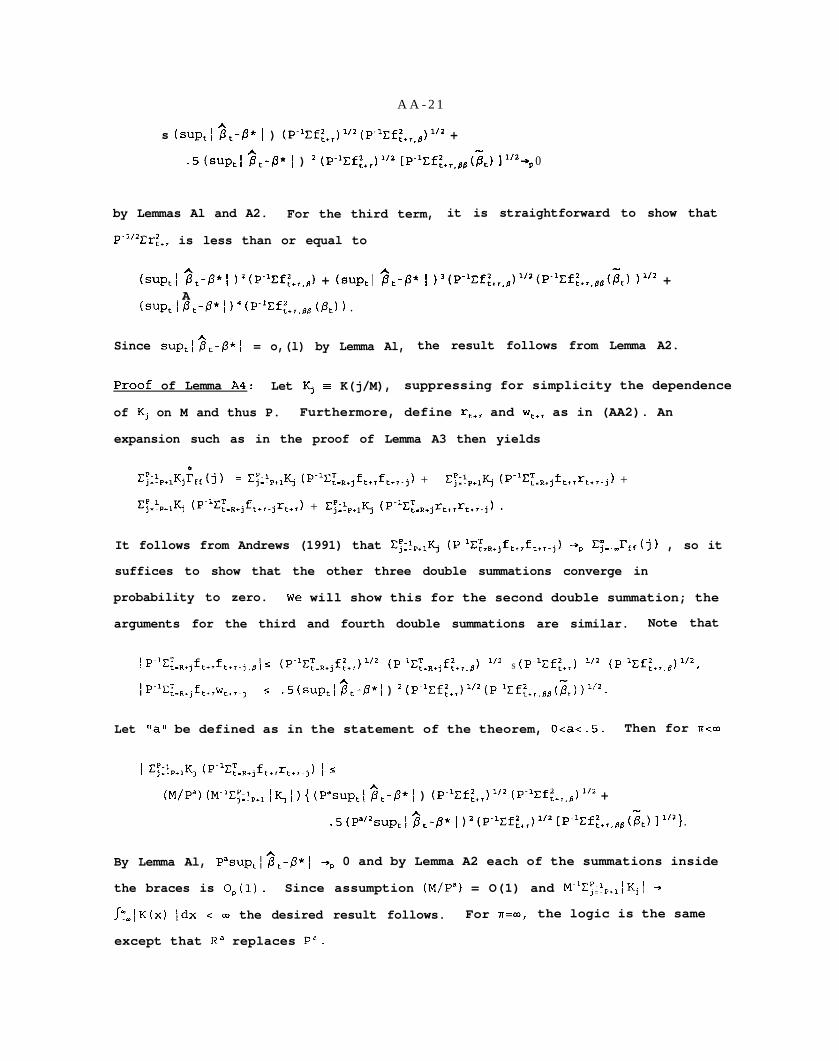
A A - 2 1
s (sup,! 2,-p* 1 ) (P-'~f:+,)"2(P'l~f:+,,B)"2 +
.5 (sup,1 2,-p* 1 ) 2 (P-?Ef:+,)1'2 [P-'Cf:+,,88(Bt) 11’2 +p 0
by Lemmas Al and A2. For the third term, it is straightforward to show that
p-l/2zr2trr is less than or equal to
(sup,\ 2,-p*; )2(P-'cf:+,,,) + (sup,] 3,-p* 1 )'(P-l~f:+~,B)1/2(P-1Zf:+,,BB(jjt) )1'2 +A
(SUPt I P,-p* f ) 4 (P-‘Cf:+,,,, (P,) 1 .
Since supt/Pt-P*\ = o,(l) by Lemma Al, the result follows from Lemma A2.
Proof of Lemma A4: Let Kj E K(j/M), suppressing for simplicity the dependence
of Kj on M and thus P. Furthermore, define rt+, and wt+, as in (AA2). An
expansion such as in the proof of Lemma A3 then yields
~$i,+lKj~ff Cj ) = cTi!,+,Kj (P-lCT_R+jft+Tft+r-j) + Cp;l-p+,Kj (P-lCT-,+jf,+,r,+,.j) +
cpi’,+IKj (P-l~TI,+jft+,.jrt+r) + Cp;T,+,Kj (P-lCT,R+jTt+rTf+r.j) -
It follows from Andrews (1991) that CP;!,+,q (P-l~~=~+jft+rft+r.j) +p E;=.,I',,(j) , so it
suffices to show that the other three double summations converge in
probability to zero. We will show this for the second double summation; the
arguments for the third and fourth double summations are similar. Note that
1 P-lZ*t.R+jft+rft+r.j,Bl s (P-1CT=,+jf:+r)1'2 (P-'CT=,+jf:+,,fl) l/2 S (P-'Cf:,,) 1'2 (P-1Cf:+,,,)"2,
IP-'ETt=R*jft+rWt+r-j I s .5 (sup,! $,-p* 1 ) 2(P-1Zf:+,)1'2 (P-lCf:,,,,, (Z,) )l'2.
Let "al' be defined as in the statement of the theorem, Ocac.5. Then for ~crn
1 E~ilp+lKj (P-lET=,+jft+,rt+,~j) 1 S
(M/Pa) @J-'E&+~ 1 q 1 ) { (P"sup,l pt-p* 1 ) (P-1Cf:+,)1'2 (P-lEf:+,,,Y2 +
.5(P"'%up,I 2,-p* 1 )2(P-%f:+,)1'2 WEf:+,,,,G,) 11’2} .
By Lemma Al, Pasupt~~,-fl*\ +p 0 and by Lemma A2 each of the summations inside
the braces is O,(l). Since assumption (M/Pa) = O(1) and M~lZ~:i,+l~K\ --,
k,\K(x) /dx < co the desired result follows. For r=m, the logic is the same
except that Ra replaces Pa.
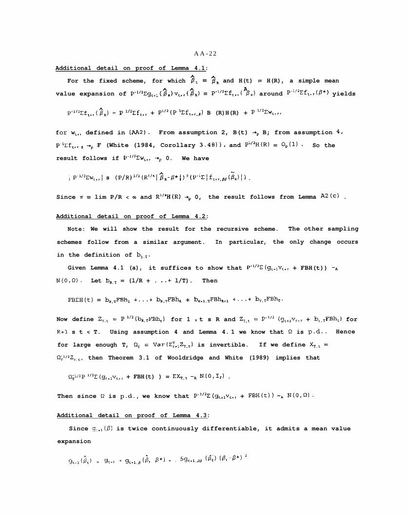
A A - 2 2
Additional detail on proof of Lemma 4.1:
For the fixed scheme, for which pt = 3, and H(t) E H(R), a simple mean
Avalue expansion of P-1~2~g,+l(~,)v~+,(~,) = P-1'2Cf,+,( PR) around P-"2Cf,+,(P*) yields
p-"2cf,+,($R) = P-1'2Cf,+, + P1'2(P-1Cft+r,B) B (R)H(R) + P-1'2Zwt+r,
for w,,, defined in (AA2). From assumption 2, B(t) -Q B; from assumption 4,
P-?zf,+, fl --,p F (White (1984, Corollary 3.48)), and P1'2H(R) = G,(l) - So the
result follows if P-l"Zw,,, jp 0. We have
1 P-"%W,,,/ s (P/R)1'2(R1'41 &+ 1 )2(P-1Clft+,,ss(iR) I) .
Since 77 E lim P/R < cn and Rw4H(R) -Q 0, the result follows from Lemma A2(c) .
Additional detail on proof of Lemma 4.2:
Note: We will show the result for the recursive scheme. The other sampling
schemes follow from a similar argument. In particular, the only change occurs
in the definition of bj,=,
Given Lemma 4.1 (a), it suffices to show that P-1'2E(gt+lvt+r + FBH(t)) -R
N(O,Q). Let b,., = (l/R + . ..+ l/T). Then
FBEH(t) = b,,,FBh, +...+ b,,,FBh, + b,+,,,FBh,+, +...+ b,,,FBh,.
Now define Z,,, = P-1/2(bR,T FBh,) for 1 s t s R and Z,,, = P-II2 (g,+lv,+, + b,,.FBh,) for
R+l s t B T. Using assumption 4 and Lemma 4. 1 we know that R is p.d.. Hence
for large enough T, Q, z Var(ZzWIZT,t) is invertible. If we define XT,, =
R,l/2Z Tt, then Theorem 3.1 of Wooldridge and White (1989) implies that
R,1W1'2E(gt+lvt+i + FBH(t) ) = XX,,, -& N(O,I,) .
Then since R is p-d., we know that P-"2E(gt+lvt+, + FBH(t)) -& N(O,R).
Additional detail on proof of Lemma 4.3:
Since g,+,(p) is twice continuously differentiable, it admits a mean value
expansion
g,*,&) = %+1
Y *
+ gt+l,B ($,-/?*I + . %+1.68 (Pt) (pt-p*) 2

AA-23
and hence
p-lxg:+,(;,) = p-1cg:+, + P-'/T{g:+,,8(j&3*)2 + .25d+1,88(&) (h*)' +
2gt+~~t+l.~(ii-P*) + gt+lgt+l,8fl (;,I t&-P*) 2 + 2%*1.89t+1.88 (i?t) @t-p*) '1
c p-1xg:+, + P-lZwt+l.
Now since g,+I is fourth order stationary and has 8d moments, Chebyshev's
inequality implies that P“Eg:+, +p Eg:+,.
To show that Pm'Cw,,, = o,(l) we use the triangle and Cauchy-Schwarz
inequalities to obtain
I P-YEW,,, ; s (sup,l&-P* I )2(p-1%J:+l,s) +
(sup,~~,-P*l)'[p'~g:+,,B,(P,)) +
2(sup,&p*;) (P-11Zg:+,)1'2 w1~LI:+l,y2 +
(sup,1 j&3* 1 ) 2 (P-'cg:+,)1'2 wcg:+,,B,(Bt) )1'2 +
2 (sup, 1 it-p* I ) 3 (P-‘~g:+,,,) 1’2 wQ3:+,,,, (Pt) ) 1’2
Since sup,I;,-p*1 = o,(l) by Lemma Al, and P-'Xg:,,,,, ('ii,) = O,(l) by assumption
3, and the remaining terms are O,(l) by assumption 4 and Markov's inequality,
the result is established.
Additional detail on proof of Theorem 4.2(b) :
Expanding qt+, we have
A AA A h A
p-lxTtSR+jgt*lgt+l-j (17t+,rlt+~-j - Vt-j.t+rVt.t+r-j) =
P~l~T-~+j{-Agt+l.jAg:+l~t.j,L+r-j~ - $t+lG:+l.j$t,t+r' + ~~+l~'~~+l-j~
E p-lx:Tt.R+jWt+l-j
(AA3)
Via the triangle and Cauchy-Schwarz inequalities we have
I P-T ’td+jwt+l-j I S (P-‘~T-,+j~:+1.j~:.j,t+~.j) 1’2 tPw’ETm,+jG2h9:+l) 1’2 +
(P~'CT~,+j~~+1AV~,t+r)1'2(P~1C~;R+j~2Ag~+l-j)1'2 +
A A A4(P-lXT,,+j cY4g:+l) 1'2 (PelEF=R+j gt+l-j) 1'2
As Ia I (P~lC;:+l&+,)1'2 (P-l&+,) 1'2 +
I o!, (P-'c;;:+,v:,,*,)'/2(P-lz~:+l)1'2*I A + ~2(P-'c~4,+,) U2 (P-&+J1'2
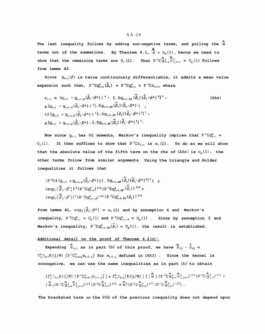
A A - 2 4
The last inequality follows by adding non-negative terms, and pulling the 2A
terms out of the summations. By Theorem 4.1, Q = o,(l), hence we need toA
show that the remaining terms are O,(l). That Pm'EG:+,v:,,+, = O,(l) follows
from Lemma A3.
Since g,+,(p) is twice continuously differentiable, it admits a mean value
expansion such that, P‘lCg:+l($,) = P-lCgz+, + P-lBrt,l, where
r t+1 = [%+I + gt+l,B t&-P*) 1 4 + 1 - %I,+,,,, GJ (ii-P*) “I 4 +
4 [%+1 + gt+l,fl (6,-P*, 1 3 1 -CL+,,,, Gt) (k-P*) ‘1 +
12 [%+l + gt+l,8 ($,-p*, 1 2 [. %t+,,,, (Pt) k-P*) 2l 2 +
4 [gt+1 + gt+l,s(~t-P*) 1 L5gt+1,B,(SJ &-@*)"I 3.
mA4)
Now since g,+I has Ed moments, Markov's inequality implies that P-lBg:+l =
O,(l) . It then suffices to show that P-lCrt+l is o,(l). To do so we will show
that the absolute value of the fifth term on the rhs of (AA41 is o,(l), the
other terms follow from similar arguments. Using the triangle and Holder
inequalities it follows that
I P‘lE4 [g,+, + c&+1,@ (5,-P*) I r . sg,,,.,, k k-P*) 2l 3 I s
(sup,; &-P'l 1 6(P-1~g:+l)1'Q(P-1~g:+1,~~ (;?,I 1 3'4 +
(sup,1 ;,-p*; l'(P-1cg:+J'4 (P-'Eg:+,,,,(Pt) ) "*
From Lemma Al, SUP~~$~-/?*! = o,(l) and by assumption 4 and Markov's
inequality, P-'Eg~+, = O,(l) and Pm'Cgz,,,, = O,(l) . Since by assumption 3 and-
Markov's inequality, P-1Cg~+,,88(&) = O,(l), the result is established.
Additional detail on the proof of Theorem 4.2(c):
Expanding ;t+r as in part (b) of this proof, we have 2,f - 6,, =
ET;!,+,K(j/M) {P-lE~=,+jwt+l.j} for wt+I-j defined in (AA31 . Since the kernel is
nonnegative, we can use the same inequalities as in part (b) to obtain
\ET:!p+lK(j/M) {P-lET=,+jw,+,.j} 1 s Ep:l,+,IK(j/M) i { !G I (P~'~hg~+,~:,t+,)1'2(P~'C~:+,)1'2 +
1 G I (P-lE;:+,c;:,t+,)"2 (P~%;:+l)1'2 + G2(P-'c$:+,)1'2 (P-1&+l)1'2} .
The bracketed term on the EHS of the previous inequality does not depend upon
AA-25
j and so it is unaffected by the outer summand. The RHS of the inequality is
then less than or equal to
(M/Pa) (M-lXy;:,+l[K(j/M) f ) { [Pa2 1 (P-'~;;:,,~:,,+,)1'2(P-1~~:+1)1'2 +A
iP"G 1 (P-1&+1v:,t+,)1'2 (P-'c;:+l)"2 + (P"/2~)2(P-1~;;:+1)1'2(P-l~A9:+l)1'2}
where Ita" is defined as in the statement of the theorem, Ocac.5. BY
assumption (M/P') = O(1) and (M-~CT;~,+,IK(~/M) 1) + h,IK(X) I& < Q)- Notice also
that by Theorem 4.1, Pa2 = o,(l). That the RHS is o,(l) then follows from the
same argument used in (b).
Additional References
Hall, Peter and Christopher C. Heyde (1980): Martinqale Limit Theory and ItsApplication, New York: Academic Press.
White, Halbert (1984): Asymptotic Theory for Econometricians, New York:Academic Press.
References
Akgiray, Vedat (1989): "Conditional Heteroskedasticity in Time Series of StockReturns: Evidence and Forecasts," Journal of Business, 62, 55-80.
Andrews, Donald W.K. (1991): "Heteroskedasticity and Autocorrelation ConsistentCovariance Matrix Estimation," Econometrica, 59, 1465-1471.
Ashley, R., Granger, Clive W. J. and Richard Schmalansee (1980): "Advertisingand Aggregate Consumption: An Analysis of Causality," Econometrica 48,1149-1167.
Berger, Allen and Spencer Krane (1985): "The Informational Efficiency ofEconometric Model Forecasts," Review of Economics and Statistics, 67, 128-134.
Chong, Yock Y. and David F. Hendry (1986): "Econometric Evaluation of LinearMacro-Economic Models," Review of Economic Studies, 53, 671-690.
Clark, Todd (1997): "Finite-Sample Properties of Tests for ForecastEquivalence", manuscript, Federal Reserve Bank of Kansas City.
Davidson, Russell and James G. MacKinnon (1984): "Model Specification TestsBased on Artificial Linear Regressions," International Economic Review, 25,485-502.
-__---_---_ (1989) : "Testing for Consistency Using Artificial Regressions,"Econometric Theory, 5, 363-384.
Diebold, Francis X. and Robert S. Mariano (1996) : "Comparing PredictiveAccuracy," Journal of Business and Economic Statistics, 13, 253-263.
Diebold, Francis X. and James Nason (1990): "Nonparametric Exchange RatePrediction?", Journal of International Economics, 28, 315-322.
Fair, Ray C. and Robert Shiller (1990): "Comparing Information in Forecastsfrom Econometric Models," American Economic Review, 80, 375-389.
Hoffman, Dennis and Adrian Pagan (1989): "Practitioners Corner: Post-SamplePrediction Tests for Generalized Method of Moments Estimators," Oxford Bulletinof Economics and Statistics 51, 333-343.
Howrey, Philip E., Lawrence R. Klein and Michael D. McCarthy (1974) : "Notes onTesting the Predictive Performance of Econometric Models," InternationalEconomic Review, 15, 366-383.
Makridakis, Spiros et. al. (1982): "The Accuracy of Time Series Methods: TheResults from a Forecasting Competition," Journal of Forecasting, 1, 111-153.
McCracken, Michael W. (1996): "Data Mining and Out of Sample Inference,"manuscript, University of Wisconsin.
Meese, Richard A. and Kenneth Rogoff (1983) : "Empirical Exchange Rate Models ofthe Seventies: Do they Fit Out of Sample?", Journal of International Economics,14, 3-24.

----------- (1988): "Was It Real? The Exchange Rate-Interest Differential
_ Relation Over the Modern Floating-Rate Period II, Journal of Finance, 43, 933-948.
Mincer, Jacob and Victor Zarnowitz (1969): "The Evaluation of EconomicForecasts," in J. Mincer (ed.) Economic Forecasts and Expectations, New York:National Bureau of Economic Research.
Nelson, Charles R. (1972): "The Predictive Performance of the FRB-MIT-PENNModel of the U.S. Economy,l' American Economic Review, 902-917.
Newey, Whitney K. and Kenneth D. West (1994): "Automatic Lag Selection inCovariance Matrix Estimation," Review of Economic Studies, 61, 631-654.
Pagan, Adrian R. and Anthony D. Hall (1983): "Diagnostic Tests as ResidualAnalysis," Econometric Reviews, 2, 159-218.
Pagan, Adrian R. and G. William Schwert (1990) : "Alternative Models forConditional Stock Volatility," Journal of Econometrics, 45, 267-290.
West, Kenneth D. (1996): "Asymptotic Inference About Predictive Ability,"Econometrica, 64, 1067-1084.
West, Kenneth D. and Dongchul Cho (1995): "The Predictive Ability of SeveralModels of Exchange Rate Volatility," Journal of Econometrics, 69, 367-391.
West, Kenneth D. and David W. Wilcox (1996): "A Comparison of AlternativeInstrumental Variables Estimators of a Dynamic Linear Model," Journal ofBusiness and Economic Statistics, 14, 281-293.
White, Halbert (1980): "A Heteroskedasticity-Consistent Covariance MatrixEstimator and a Direct Test for Heteroskedasticity," Econometrica, 48, 817-838.
Wooldridge, Jeffrey M. (1990): "A Unified Approach to Robust, Regression-BasedSpecification Tests," Econometric Theory, 6, 17-43.
----------- (1991): "On the Application of Robust, Regression-Based Diagnosticsto Models of Conditional Means and Conditional Variances," Journal ofEconometrics, 47, 5-46.
Wooldridge, Jeffrey M. and Halbert White (1989): I'Central Limit Theorems forDependent, Heterogeneous Processes with Trending Moments," manuscript, MichiganState University.
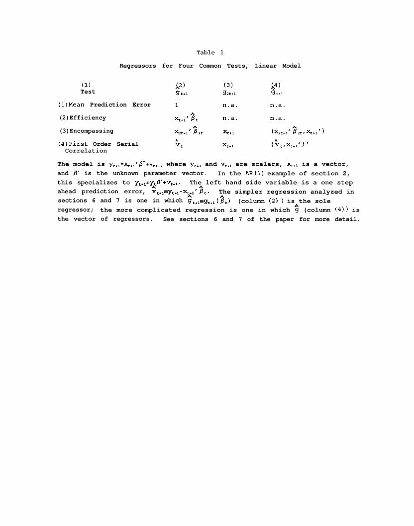
Table 1
Regressors for Four Common Tests, Linear Model
(1) x2 ) (3) A-4)Test g t*1 g2t+1 gt+1
(1)Mean Prediction Error 1 n.a. n.a.
(2)Efficiency n-a. n.a.
(3)Encompassing
(4)First Order SerialCorrelation
Xx+1 ' T&t xt+1 (xx+1 ' ii x,+*1 '1
A A
Vt xr+l (vtr++l ) '
The model is ~~+~=q+~'fi*+v~+~, where yt+l and v~+~ are scalars, q+1 is a vector,
and 0' is the unknown parameter vector. In the AR(l) example of section 2,
this specializes to ~~+~=y~p'+v~+~. The left hand side variable is a one step
ahead prediction error, ~~+~=y~+~-q+~'~~. The simpler regression analyzed in
sections 6 and 7 is one in which ^g ,+,=g,+,(~,) (column (2) 1 is the sole
regressor; the more complicated regression is one in which $ (column (4)) is
the vector of regressors. See sections 6 and 7 of the paper for more detail.
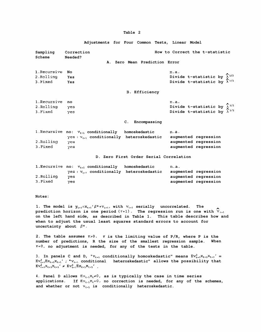
Table 2
Adjustments for Four Common Tests, Linear Model
Sampling Correction How to Correct the t-statisticScheme Needed?
A. Zero Mean Prediction Error
l.Recursive No2.Rolling Yes3.Fixed Yes
n.a.Divide t-statistic by ?I"
"l/2Divide t-statistic by X
B. Efficiency
l.Recursive no n.a.2.Rolling yes Divide t-statistic by T1j23.Fixed yes Divide t-statistic by t112
C. Encompassing
l.Recursive no: vtrl conditionally homoskedastic n-a.
yes : vt+l conditionally heteroskedastic augmented regression2.Rolling yes augmented regression3.Fixed yes augmented regression
D. Zero First Order Serial Correlation
l.Recursive no: v~+~ conditionally homoskedastic n-a.
yes = vt+l conditionally heteroskedastic augmented regression2.Rolling yes augmented regression3.Fixed yes augmented regression
Notes:
1. The model is yt+1=xt+1 'P*+v~+~, with v~+~ serially uncorrelated. Theprediction horizon is one period (~=l). The regression run is one with c,+,on the left hand side, as described in Table 1. This table describes how andwhen to adjust the usual least squares standard errors to account foruncertainty about p*.
2. The table assumes a>O. TT is the limiting value of P/R, where P is thenumber of predictions, R the size of the smallest regression sample. WhenPO, no adjustment is needed, for any of the tests in the table.
3. In panels C and D, "v~+~ conditionally homoskedastic" means Ev:+~x~+~++~' =
Ev:+J%+lxt+l' ; "vt+l conditional heteroskedastic" allows the possibility that
Ev:+lxt+lxt+l' f Ev:+,Ext+1xt+,' .
4. Panel D allows Ev~+~x~zO, as is typically the case in time seriesapplications. If Ev~+~x~=O, no correction is needed, for any of the schemes,and whether or not v~+~ is conditionally heteroskedastic.
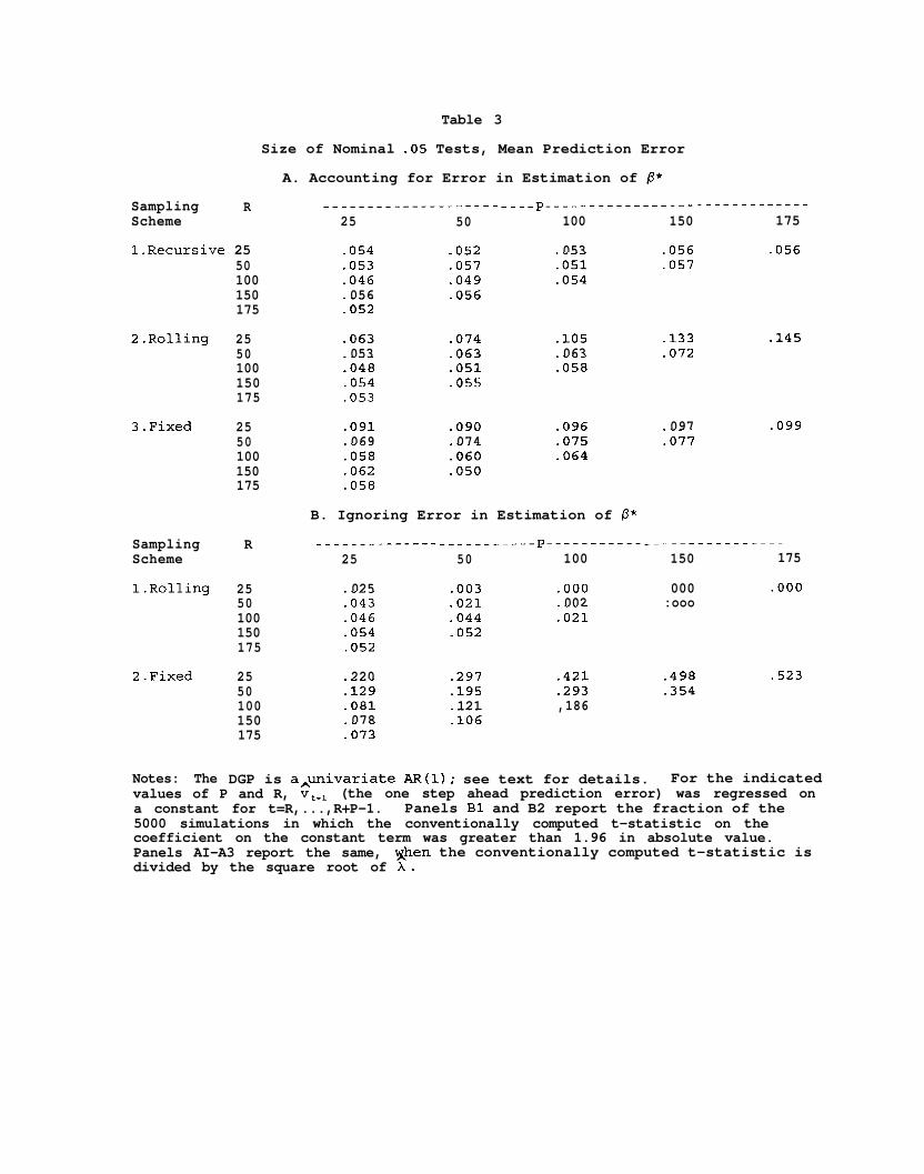
Table 3
Size of Nominal .05 Tests, Mean Prediction Error
A. Accounting for Error in Estimation of p*
Sampling RScheme
l.Recursive 25
2.Rolling
3.Fixed
SamplingScheme
l.Rolling
2.Fixed
50100150175
2550100150175
2550100150175
R
2550100150175
2550100150175
-----___--_____----- ----p------------------------------25 50 100
-054 -052 053.053 -057 :051.046 .049 .054056:052
.056
150 175
.056 .056
.057
.063 .074 .105053:048
-063 063.051 :058
.054 .055
.053
-133 .145.072
.091 -090 .096069:058
074:060
.075
.064.062 .050-058
097:077
.099
B. Ignoring Error in Estimation of fl*
__-----_------ -----------p-----------25 50 100
--
0251043
.003 -000
.021 002.046 .044 :021.054 .052.052
220:129
.297 .421
.195 .293.081 121 ,186078:073
:106
___-___-___-----150 175
000:ooo
-000
.498 -523-354
Notes: The DGP is a,univariate AR(l); see text for details. For the indicatedvalues of P and R, v,,, (the one step ahead prediction error) was regressed ona constant for t=R,...,R+P-1. Panels Bl and B2 report the fraction of the5000 simulations in which the conventionally computed t-statistic on thecoefficient on the constant term was greater than 1.96 in absolute value.Panels AI-A3 report the same, xhen the conventionally computed t-statistic isdivided by the square root of X.

Table 4
Size of Nominal -05 Tests, Efficiency Test
A. Accounting for Error in Estimation of fi*
Sampling R ----------____----- ------p-----------------------------Scheme - 25 50 100
l.Recursive 25 .052 .051 .05550 .038 .043 .043100 .038 .040 -045150 .041 .047175 .042
150 175
.055 .053
.046
2.Rolling
3.Fixed
SamplingScheme
l.Rolling
2.Fixed
2550100150175
25 .058 .055 -05650 .040 038
:041.035
100 .039 .042150 .041 .036175 .042
R
25 .059 .072 15250 .037 .030 :016100 .034 034150 :041
.021.042
175 .040
25 .158 .234 -35550 .087 .135 .220100 .063 097150 :083
-152.060
175 .057
124:045
-430 .939.070 .232
.036 .043 .059-042 .045.041
B. Ignoring Error in Estimation of p*
-------------------------p-------------25 50 100
.997 .999
.468
.055 -053
.031
.434 .456
.286
Notes: The DGP is a,univariate AR(l); see text for details. For the indicatedvalues of P and,R, vtrl (the one step ahead prediction) was regressed on aconstant and y,fl, (the one step ahead prediction) for t=R, . . ..R+P-1. PanelsBl and B2 report the fraction of the 5000 simulations in whigh theconventionally computed t-statistic on the coefficient on y,p, that wasgreater than 1.96 in absolute value. Panels Al-A3 report the same, wken theconventionally computed t-statistic is divided by the square root of A.
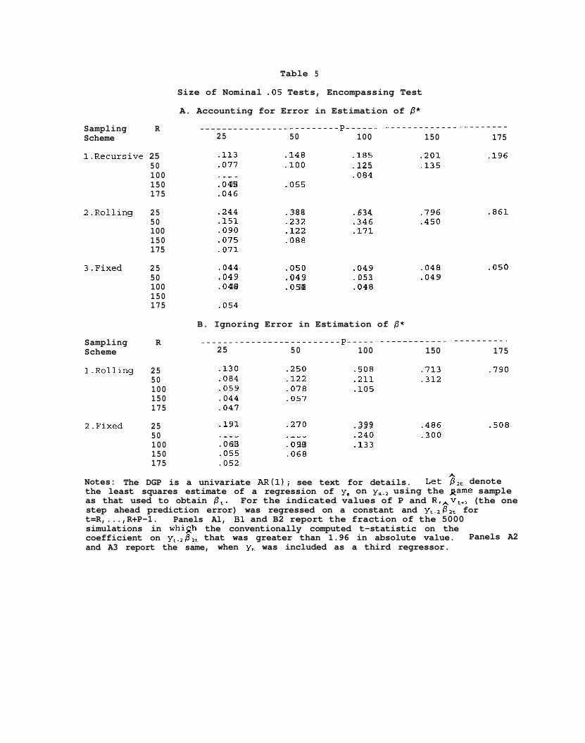
Sampling RScheme
l.Recursive 25
2.Rolling
3.Fixed
SamplingScheme
l.Rolling
2.Fixed
50100150175
-------------------------p-------------------------------25 50 100 150 175
.113 .148 .185 .201 .196
.077 .lOO 125 .135
:045 054 .070 .055:084
.046
2550100150175
.244 388 .861
.151 :232634:346
.796
.450.090 .122 .171-075 .088.071
2550100150175
.044 .050 .049 .048 .050
.049 .049 053:049 049 :051 048 :048
-049
.054
B. Ignoring Error in Estimation of /L?*
R -------------------------p-------------------------------25 50 100 150 175
25 -130 .250 .508 .713 .79050 .084 .122 .211 .312100 .059 .078 -105150 -044 -057175 .047
2550100150175
.191 .270 399 -486 .508
:063 103 :093 160:240 .300-133
.055 .068
.052
Table 5
Size of Nominal .05 Tests, Encompassing Test
A. Accounting for Error in Estimation of p*
Notes: The DGP is a univariate AR(l); see text for details. Let 2,, denotethe least squares estimate of a regression of ys on ysm2 using the game sampleas that used to obtain pt. For the indicated values of P and R,,v,,, (the onestep ahead prediction error) was regressed on a constant and yt.2P2t fort=R,...,R+P-1. Panels Al, Bl and B2 report the fraction of the 5000simulations in whish the conventionally computed t-statistic on thecoefficient on yt.2P2t that was greater than 1.96 in absolute value. Panels A2and A3 report the same, when yt was included as a third regressor.
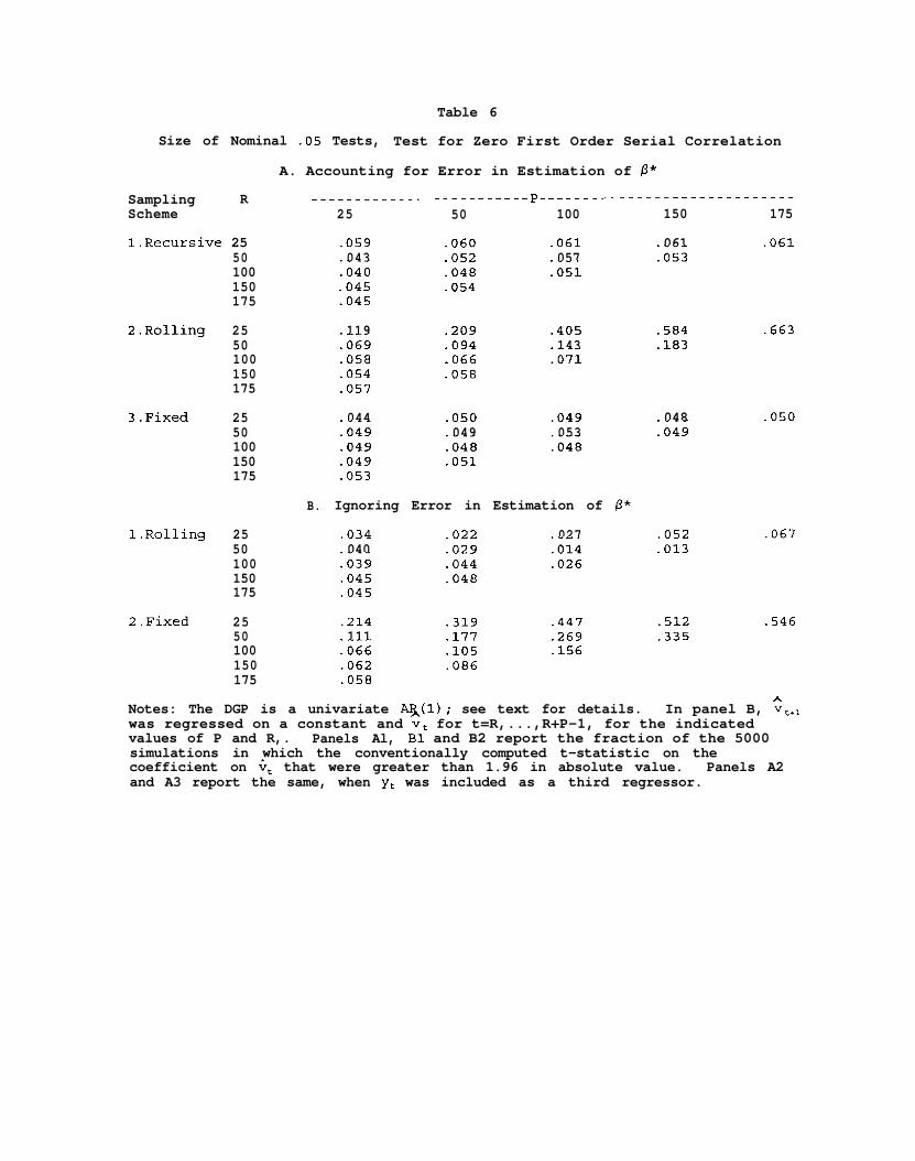
Table 6
Size of Nominal .05 Tests, Test for Zero First Order Serial Correlation
Sampling RScheme
I.Recursive 25
2.Rolling
3.Fixed
l.Rolling
2.Fixed
50100150175
2550100150175
2550100150175
2550100150175
2550100150175
A. Accounting for Error in Estimation of p*
-------------------------p-------------------------------25 50 100 150 175
.059 .060 .061 061 .061043:040
.052 057
.048 :051:053
.045 .054-045
119:069
.209 .405 .584 .663
.094 143 .183.058 .066 :071.054 .058.057
044 .050 .049 048:049
.050:049 049
:048053
.049 :048
.049 .051
.053
B. Ignoring Error in Estimation of p*
.034 .022 027 .052 .067040:039
.029 :014 .013
.044 .026.045 .048.045
.214 .319 .447 .512 .546111:066
.177 .269 .335
.105 .156.062 .086.058
hNotes: The DGP is a univariate q(l); see text for details. In panel B, vt+lwas regressed on a constant and vt for t=R,...,R+P-1, for the indicatedvalues of P and R,. Panels Al, Bl and B2 report the fraction of the 5000simulations in which the conventionally computed t-statistic on thecoefficient on Gt that were greater than 1.96 in absolute value. Panels A2and A3 report the same, when yt was included as a third regressor.
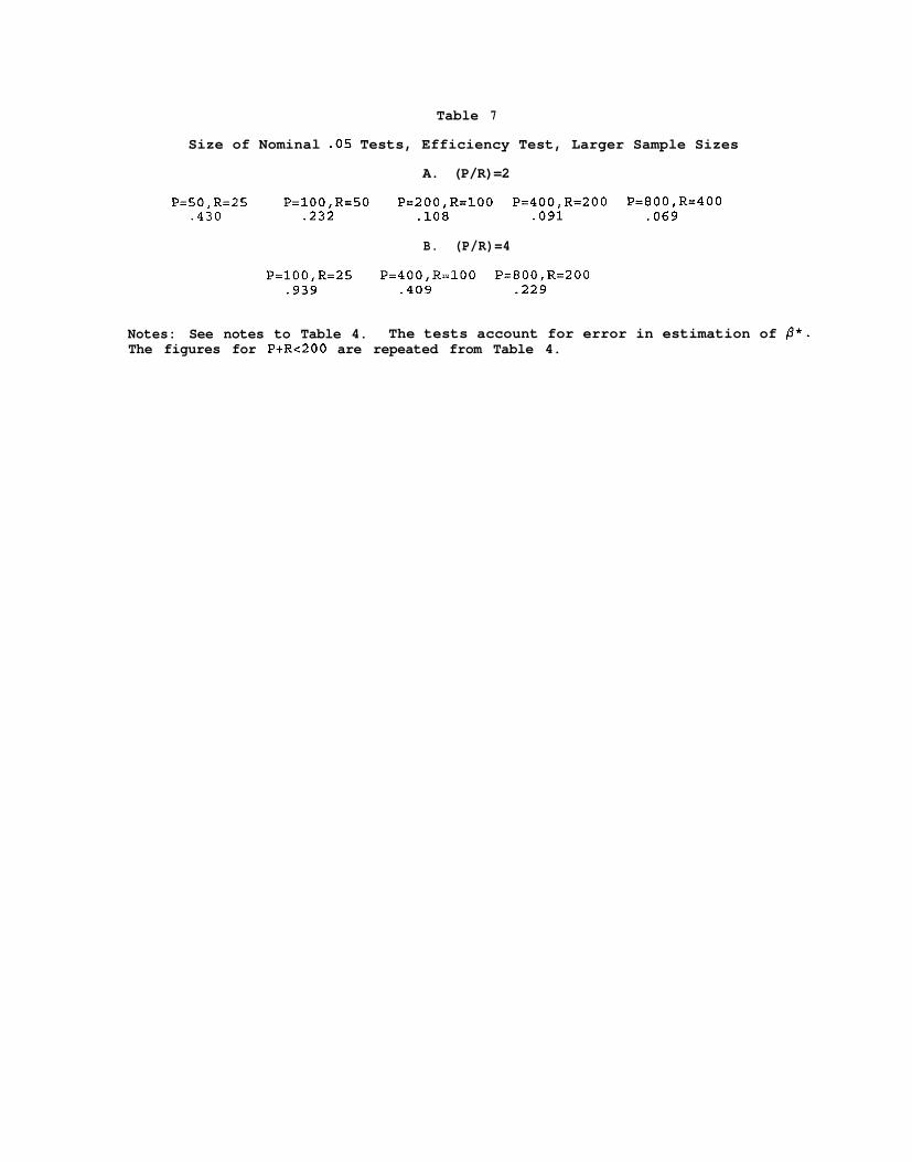
Table 7
Size of Nominal .05 Tests, Efficiency Test, Larger Sample Sizes
A. (P/R)=2
P=50,R=25 P=lOO,R=50 P=200,R=lOO P=400,R=200 P=800,R=400.430 .232 -108 .091 .069
B. (P/R)=4
P=lOO,R=25 P=400,R=lOO P=800,R=200.939 .409 -229
Notes: See notes to Table 4. The tests account for error in estimation of p*.The figures for P+Rc200 are repeated from Table 4.