Embed Size (px)
Citation preview
ERD
C/EL
TR-
12-1
Wetlands Regulatory Assistance Program
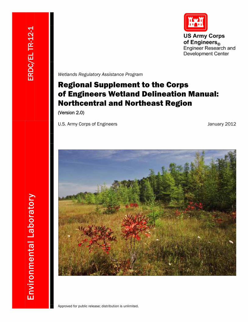
Regional Supplement to the Corps of Engineers Wetland Delineation Manual: Northcentral and Northeast Region (Version 2.0)
Envi
ronm
enta
l Lab
orat
ory
U.S. Army Corps of Engineers January 2012
Approved for public release; distribution is unlimited.
Wetlands Regulatory Assistance Program ERDC/EL TR-12-1 January 2012
Regional Supplement to the Corps of Engineers Wetland Delineation Manual: Northcentral and Northeast Region (Version 2.0)
U.S. Army Corps of Engineers U.S. Army Engineer Research and Development Center 3909 Halls Ferry Road Vicksburg, MS 39180-6199
Final report Approved for public release; distribution is unlimited.
Prepared for Headquarters, U.S. Army Corps of Engineers Washington, DC 20314-1000
ERDC/EL TR-12-1 ii
Abstract: This document is one of a series of Regional Supplements to the Corps of Engineers Wetland Delineation Manual, which provides technical guidance and procedures for identifying and delineating wet-lands that may be subject to regulatory jurisdiction under Section 404 of the Clean Water Act or Section 10 of the Rivers and Harbors Act. The development of Regional Supplements is part of a nationwide effort to address regional wetland characteristics and improve the accuracy and efficiency of wetland-delineation procedures. This supplement is appli-cable to the Northcentral and Northeast Region, which consists of all or portions of 15 states: Connecticut, Illinois, Indiana, Maine, Massachusetts, Michigan, Minnesota, New Hampshire, New Jersey, New York, Ohio, Pennsylvania, Rhode Island, Vermont, and Wisconsin.
DISCLAIMER: The contents of this report are not to be used for advertising, publication, or promotional purposes. Citation of trade names does not constitute an official endorsement or approval of the use of such commercial products. All product names and trademarks cited are the property of their respective owners. The findings of this report are not to be construed as an official Department of the Army position unless so designated by other authorized documents. DESTROY THIS REPORT WHEN NO LONGER NEEDED. DO NOT RETURN IT TO THE ORIGINATOR.
ERDC/EL TR-12-1 iii
Contents Figures and Tables ................................................................................................................................ vii
Preface ....................................................................................................................................................xi
1 Introduction ..................................................................................................................................... 1
Purpose and use of this regional supplement ........................................................................ 1 Applicable region and subregions ........................................................................................... 3 Physical and biological characteristics of the region ............................................................. 5
Northcentral Forests (LRR K) ...................................................................................................... 8 Central Great Lakes Forests (LRR L) ........................................................................................... 8 Northeastern Forests (LRR R) ..................................................................................................... 9 Long Island/Cape Cod (MLRA 149B) .......................................................................................... 9
Types and distribution of wetlands ........................................................................................ 10
2 Hydrophytic Vegetation Indicators ............................................................................................. 15
Introduction ............................................................................................................................ 15 Guidance on vegetation sampling and analysis ................................................................... 17
Definitions of strata ................................................................................................................... 18 Plot and sample sizes ................................................................................................................ 18 Seasonal considerations and cautions ..................................................................................... 21
Hydrophytic vegetation indicators ......................................................................................... 22 Procedure ................................................................................................................................... 24 Indicator 1: Rapid test for hydrophytic vegetation ................................................................... 25 Indicator 2: Dominance test ...................................................................................................... 25 Indicator 3: Prevalence index .................................................................................................... 27 Indicator 4: Morphological adaptations .................................................................................... 30
3 Hydric Soil Indicators ................................................................................................................... 32
Introduction ............................................................................................................................ 32 Concepts ................................................................................................................................. 33
Iron and manganese reduction, translocation, and accumulation ......................................... 33 Sulfate reduction ........................................................................................................................ 34 Organic matter accumulation .................................................................................................... 34
Cautions .................................................................................................................................. 36 Procedures for sampling soils ............................................................................................... 37
Observe and document the site ................................................................................................ 37 Observe and document the soil ................................................................................................ 39
Use of existing soil data ......................................................................................................... 41 Soil surveys ................................................................................................................................. 41 Hydric soils lists .......................................................................................................................... 41
Hydric soil indicators .............................................................................................................. 42 All soils ........................................................................................................................................ 44
Indicator A1: Histosol ..................................................................................................... 44
ERDC/EL TR-12-1 iv
Indicator A2: Histic Epipedon ........................................................................................ 46 Indicator A3: Black Histic ............................................................................................... 47 Indicator A4: Hydrogen Sulfide ...................................................................................... 47 Indicator A5: Stratified Layers ....................................................................................... 48 Indicator A11: Depleted Below Dark Surface ............................................................... 49 Indicator A12: Thick Dark Surface ................................................................................ 50
Sandy soils .................................................................................................................................. 51 Indicator S1: Sandy Mucky Mineral .............................................................................. 52 Indicator S4: Sandy Gleyed Matrix ................................................................................ 53 Indicator S5: Sandy Redox............................................................................................. 54 Indicator S6: Stripped Matrix ......................................................................................... 55 Indicator S7: Dark Surface ............................................................................................ 56 Indicator S8: Polyvalue Below Surface ......................................................................... 57 Indicator S9: Thin Dark Surface .................................................................................... 59
Loamy and clayey soils .............................................................................................................. 61 Indicator F1: Loamy Mucky Mineral .............................................................................. 61 Indicator F2: Loamy Gleyed Matrix ................................................................................ 61 Indicator F3: Depleted Matrix ........................................................................................ 63 Indicator F6: Redox Dark Surface ................................................................................. 64 Indicator F7: Depleted Dark Surface ............................................................................. 66 Indicator F8: Redox Depressions .................................................................................. 67
Hydric soil indicators for problem soils ................................................................................. 68 Indicator A10: 2 cm Muck ............................................................................................. 68 Indicator A16: Coast Prairie Redox ............................................................................... 69 Indicator S3: 5 cm Mucky Peat or Peat ......................................................................... 69 Indicator S7: Dark Surface ............................................................................................ 70 Indicator S8: Polyvalue Below Surface ......................................................................... 70 Indicator S9: Thin Dark Surface .................................................................................... 71 Indicator F12: Iron-Manganese Masses ....................................................................... 71 Indicator F19: Piedmont Floodplain Soils ..................................................................... 72 Indicator F21: Red Parent Material ............................................................................... 73 Indicator TA6: Mesic Spodic .......................................................................................... 74 Indicator TF12: Very Shallow Dark Surface .................................................................. 75
4 Wetland Hydrology Indicators ..................................................................................................... 76
Introduction ............................................................................................................................ 76 Growing season ...................................................................................................................... 78 Wetland hydrology indicators ................................................................................................. 81
Group A – Observation of Surface Water or Saturated Soils ................................................... 83 Indicator A1: Surface water ........................................................................................... 83 Indicator A2: High water table ....................................................................................... 84 Indicator A3: Saturation ................................................................................................. 85
Group B – Evidence of Recent Inundation ............................................................................... 86 Indicator B1: Water marks ............................................................................................. 86 Indicator B2: Sediment deposits ................................................................................... 87 Indicator B3: Drift deposits ............................................................................................ 88 Indicator B4: Algal mat or crust ..................................................................................... 89 Indicator B5: Iron deposits ............................................................................................ 90 Indicator B7: Inundation visible on aerial imagery ....................................................... 92
ERDC/EL TR-12-1 v
Indicator B8: Sparsely vegetated concave surface ...................................................... 93 Indicator B9: Water-stained leaves ............................................................................... 94 Indicator B13: Aquatic fauna ......................................................................................... 94 Indicator B15: Marl deposits ......................................................................................... 96 Indicator B6: Surface soil cracks ................................................................................... 96 Indicator B10: Drainage patterns .................................................................................. 98 Indicator B16: Moss trim lines .................................................................................... 100
Group C – Evidence of Current or Recent Soil Saturation ..................................................... 101 Indicator C1: Hydrogen sulfide odor ............................................................................ 101 Indicator C3: Oxidized rhizospheres along living roots............................................... 101 Indicator C4: Presence of reduced iron ...................................................................... 103 Indicator C6: Recent iron reduction in tilled soils ...................................................... 104 Indicator C7: Thin muck surface ................................................................................. 105 Indicator C2: Dry-season water table .......................................................................... 106 Indicator C8: Crayfish burrows .................................................................................... 106 Indicator C9: Saturation visible on aerial imagery ..................................................... 107
Group D – Evidence from Other Site Conditions or Data ....................................................... 109 Indicator D1: Stunted or stressed plants .................................................................... 109 Indicator D2: Geomorphic position ............................................................................. 110 Indicator D3: Shallow aquitard .................................................................................... 111 Indicator D4: Microtopographic Relief ........................................................................ 112 Indicator D5: FAC-neutral test ..................................................................................... 113
5 Difficult Wetland Situations in the Northcentral and Northeast Region ............................ 114
Introduction .......................................................................................................................... 114 Lands used for agriculture and silviculture ........................................................................ 115 Problematic hydrophytic vegetation .................................................................................... 118
Description of the problem ...................................................................................................... 118 Procedure ................................................................................................................................. 118
Problematic hydric soils ....................................................................................................... 128 Description of the problem ...................................................................................................... 128
Soils with faint or no indicators ................................................................................... 128 Soils with relict hydric soil indicators .......................................................................... 130 Non-hydric soils that may be misinterpreted as hydric .............................................. 131
Procedure ................................................................................................................................. 132 Wetlands that periodically lack indicators of wetland hydrology ....................................... 136
Description of the problem ...................................................................................................... 136 Procedure ................................................................................................................................. 137
Wetland/non-wetland mosaics ............................................................................................ 142 Description of the problem ...................................................................................................... 142 Procedure ................................................................................................................................. 143
References ......................................................................................................................................... 145
Appendix A: Glossary ........................................................................................................................ 149
Appendix B: Point-Intercept Sampling Procedure for Determining Hydrophytic Vegetation .................................................................................................................................. 156

ERDC/EL TR-12-1 vi
Appendix C: Data Form .................................................................................................................... 158
Report Documentation Page
ERDC/EL TR-12-1 vii
Figures and Tables
Figures
Figure 1. Approximate boundaries of the Northcentral and Northeast Region. Subregions used in this supplement correspond to USDA Land Resource Regions (LRR). This supplement is applicable throughout the highlighted areas, although some indicators may be restricted to specific subregions or smaller areas. See text for details. .......................................... 4
Figure 2. Suggested plot arrangements for vegetation sampling. (A) Single plots in graduated sizes. (B) Nested 3.28- by 3.28-ft square (1-m2) plots for herbs within the 30-ft radius plot. ................................................................................................................................................ 19
Figure 3. Plant list regional boundaries (red lines) currently used by the U.S. Fish and Wildlife Service, National Wetlands Inventory, in the Northcentral and Northeast Region. ............. 23
Figure 4. Shallow roots of eastern hemlock are a response to high water tables in this forested wetland. ...................................................................................................................................... 31
Figure 5. Divergent slopes (A) disperse surface water, whereas convergent slopes (B) concentrate water. Surface flow paths are indicated by the arrows. .................................................. 38
Figure 6. At the toe of a hill slope, the gradient is only slightly inclined or nearly level. Blue arrows represent flow paths of surface water and groundwater ......................................................... 39
Figure 7. Example of a Histosol, in which muck (sapric soil material) is greater than 3 ft (0.9 m) thick.............................................................................................................................................. 45
Figure 8. This Histosol consists of only a few inches of organic soil material over bedrock in a shallow glacial groove. ...................................................................................................................... 45
Figure 9. In this soil, the organic surface layer is about 9 in. (23 cm) thick. Scale is in centimeters. .............................................................................................................................................. 46
Figure 10. Stratified layers in loamy material. ....................................................................................... 48
Figure 11. Stratified layers in sandy material. ....................................................................................... 48
Figure 12. In this soil, a depleted matrix starts immediately below the black surface layer at approximately 11 in. (28 cm). ............................................................................................................. 50
Figure 13. Deep observations may be necessary to identify the depleted or gleyed matrix below a thick, dark surface layer. In this example, the depleted matrix starts at 20 in. (50 cm). ..................................................................................................................................................... 52
Figure 14. The mucky modified sandy layer is approximately 3 in. (7.5 cm) thick. Scale in inches on the right side of ruler. ............................................................................................................. 53
Figure 15. In this example, the gleyed matrix begins at the soil surface. ........................................... 54
Figure 16. Redox concentrations in sandy soil material. ...................................................................... 55
Figure 17. In this example, a faint splotchy pattern of stripped and unstripped areas lies beneath a thin dark surface layer. .......................................................................................................... 56
Figure 18. Location of MLRA 149B of LRR S......................................................................................... 58
Figure 19. Example of indicator S7 (Dark Surface) in a sandy soil. Scale in inches on right. .......... 58
Figure 20. In this soil, the splotchy pattern below the dark surface is due to mobilization and translocation of organic matter. Scale in inches. .......................................................................... 59
Figure 21. Example of indicator S9 (Thin Dark Surface). Scale in inches on right. ........................... 60
ERDC/EL TR-12-1 viii
Figure 22. This soil has a gleyed matrix in the lowest layer, starting about 7 in. (18 cm) from the soil surface. The layer above the gleyed matrix has a depleted matrix. .............................. 62
Figure 23. Example of indicator F3 (Depleted Matrix), in which redox concentrations extend nearly to the surface. ................................................................................................................... 63
Figure 24. This soil has a depleted matrix with redox concentrations in a low-chroma matrix. ........... 64
Figure 25. Redox features can be small and difficult to see within a dark soil layer. ........................ 65
Figure 26. Redox depletions are scattered within the darker matrix. Scale is in centimeters. ............ 66
Figure 27. In this example, the layer of redox concentrations begins at the soil surface and is slightly more than 2 in. (5 cm) thick. .................................................................................................. 67
Figure 28. Iron-manganese masses in a 40 percent depleted matrix. Scale is in inches. ............... 72
Figure 29. The Piedmont Floodplain Soils indicator is restricted to floodplains that are actively receiving sediments and groundwater discharge with high iron content. Photo by M. Rabenhorst. Scale in 4-in. (10-cm) increments. .............................................................................. 73
Figure 30. Location of MLRAs 144A and 145 in LRR R and MLRA 149B in LRR S. ......................... 75
Figure 31. A caution in determining the start of the growing season using the “green up” indicator. Certain herbaceous species produce overwintering green leaves. An example is Dame’s rocket (Hesperis matronalis) where the stem, stem leaves, and flowers die back at the end of the growing season, but a basal rosette of green leaves persists under the snowpack. The photograph above, which was taken immediately following the first exposure of the ground surface after snowmelt, illustrates this characteristic. ................................ 80
Figure 32. Wetland with surface water present. ................................................................................... 84
Figure 33. High water table observed in a soil pit. ................................................................................ 85
Figure 34. Water glistens on the surface of a saturated soil sample. ................................................ 86
Figure 35. Water marks on trees in a seasonally flooded wetland. .................................................... 87
Figure 36. Silt deposit left after a recent high-water event forms a tan coating on these tree trunks ................................................................................................................................................. 88
Figure 37. Drift deposit on the upstream side of a sapling in a floodplain wetland. ......................... 89
Figure 38. Dried algal deposit clinging to low vegetation. .................................................................... 90
Figure 39. Dried crust of blue-green algae on the soil surface. .......................................................... 91
Figure 40. Iron deposit (orange streaks) in a small channel. .............................................................. 91
Figure 41. At this site, ferrous iron moves with the groundwater from a cattail marsh to a shallow ditch, where it oxidizes when exposed to the air and forms an orange-colored iron deposit. ...................................................................................................................................................... 92
Figure 42. A sparsely vegetated, seasonally ponded depression. Note the watermarks on trees. .......................................................................................................................................................... 93
Figure 43. Water-stained leaves in a seasonally ponded depression, with an unstained leaf for comparison. ................................................................................................................................. 94
Figure 44. Shells of aquatic snails in a seasonally ponded fringe wetland. ....................................... 95
Figure 45. Dead green frogs (Rana clamitans melanota) in a drying seasonal pool. ....................... 96
Figure 46. Marl deposit and iron sheen in a calcareous fen. .............................................................. 97
Figure 47. Surface soil cracks in a seasonally ponded depression. .................................................... 97
Figure 48. Drainage patterns seen during typical early spring flows in a forested wetland. The patterns are also evident when the wetland is dry. ....................................................................... 98
Figure 49. Drainage patterns in a slope wetland. ................................................................................. 99
ERDC/EL TR-12-1 ix
Figure 50. Vegetation bent over in the direction of water flow across a stream terrace. .................. 99
Figure 51. Moss trim lines in a seasonally flooded wetland. Trim lines indicate a recent high-water level. ...................................................................................................................................... 100
Figure 52. Iron-oxide plaque (orange coating) on a living root. Iron also coats the channel or pore from which the root was removed. .......................................................................................... 102
Figure 53. This soil has many oxidized rhizospheres associated with living roots. ......................... 102
Figure 54. When alpha, alpha-dipyridyl is applied to a soil containing reduced iron, a positive reaction is indicated by a pink or red coloration to the treated area. ................................. 104
Figure 55. Redox concentrations in the tilled surface layer of a recently cultivated soil. ............... 105
Figure 56. Crayfish burrow in a saturated wetland. ............................................................................ 107
Figure 57. Aerial photograph of an agricultural field with saturated soils indicated by darker colors. .......................................................................................................................................... 108
Figure 58. Stunted corn due to wet spots in an agricultural field in New Hampshire. .................... 109
Figure 59. Black spruce in the wetland are stressed and stunted compared with spruce in the adjacent areas ................................................................................................................................. 110
Figure 60. Fringes of water bodies, such as this estuarine fringe, are likely to exhibit wetland hydrology. .................................................................................................................................. 111
Figure 61. This hemlock-dominated wetland has trees growing on hummocks and herbaceous plants growing in tussocks. .............................................................................................. 112
Figure 62. Effects of ditches and parallel subsurface drainage lines on the water table............... 116
Figure 63. Red areas in this photograph are iron deposits on the soil surface that are a result of high iron concentrations in the groundwater. ....................................................................... 131
Figure 64. This soil exhibits colors associated with reducing conditions. Scale is 1 cm. ............... 135
Figure 65. The same soil as in Figure 63 after exposure to the air and oxidation has occurred. ................................................................................................................................................. 135
Figure A1. Illustration of values and chromas that require 2 percent or more distinct or prominent redox concentrations and those that do not, for hue 10YR, to meet the definition of a depleted matrix. Due to inaccurate color reproduction, do not use this page to determine soil colors in the field. Background image from the Munsell Soil Color Charts reprinted courtesy of Munsell Color Services Lab, a part of X-Rite, Inc. ........................................... 152
Figure A2. For hydric soil determinations, a gleyed matrix has the hues and chroma identified in this illustration with a value of 4 or more. Due to inaccurate color reproduction, do not use this page to determine soil colors in the field. Background image from the Munsell Soil Color Charts reprinted courtesy of Munsell Color Services Lab, a part of X-Rite, Inc. .......................................................................................................................................................... 154
Tables
Table 1. Sections of the Corps Manual replaced by this Regional Supplement for applications in the Northcentral and Northeast Region. ........................................................................ 2
Table 2. Selected references to additional vegetation sampling approaches that could be used in wetland delineation. ................................................................................................................... 21
Table 3. Example of the selection of dominant species by the 50/20 rule and determination of hydrophytic vegetation by the dominance test. ....................................................... 27
Table 4. Example of the Prevalence Index using the same data as in Table 3. ................................. 29
Table 5. Proportion of sample consisting of fibers visible with a hand lens. ...................................... 35

ERDC/EL TR-12-1 x
Table 6. Determination of degree of decomposition of organic materials. ........................................ 36
Table 7. Minimum thickness requirements for commonly combined indicators in the Northcentral and Northeast Region. ...................................................................................................... 43
Table 8. Example of a soil that is hydric based on a combination of indicators F6 and F3. ............. 43
Table 9. Example of a soil that is hydric based on a combination of indicators F6 and S5. ............. 44
Table 10. Wetland hydrology indicators for the Northcentral and Northeast Region ........................ 82
Table A1. Tabular key for contrast determinations using Munsell notation...................................... 150
ERDC/EL TR-12-1 xi
Preface
This document is one of a series of Regional Supplements to the Corps of Engineers Wetland Delineation Manual. It was developed by the U.S. Army Engineer Research and Development Center (ERDC) at the request of Headquarters, U.S. Army Corps of Engineers (USACE), with funding provided through the Wetlands Regulatory Assistance Program (WRAP). This is Version 2.0 of the Northcentral and Northeast Regional Supplement; it replaces the “interim” version, which was published in October 2009.
This document was developed in cooperation with the Northcentral and Northeast Regional Working Group, whose members contributed their time and expertise to the project over a period of many months. Working Group meetings were held in Hanover, NH, on 6-8 November 2007 and Madison, WI, on 15-17 April 2008. Members of the Regional Working Group and contributors to this document were:
• James Wakeley, Project Leader and Working Group Chair, Environmental Laboratory (EL), ERDC, Vicksburg, MS
• Robert Lichvar, Chair, Vegetation Subcommittee, Cold Regions Research and Engineering Laboratory, ERDC, Hanover, NH
• Chris Noble, Chair, Soils Subcommittee, EL, ERDC, Vicksburg, MS • Edward Arthur, U.S. Army Engineer Detroit District,
Sault Ste Marie, MI • Al Averill, U.S. Department of Agriculture (USDA), Natural Resources
Conservation Service, Amherst, MA • Jacob F. Berkowitz, EL, ERDC, Vicksburg, MS • Steve Carlisle, USDA Natural Resources Conservation Service, Seneca
Falls, NY • Greg Carlson, U.S. Environmental Protection Agency, Chicago, IL • Christine Delorier, U.S. Army Engineer District, New York, NY • Steve Eggers, U.S. Army Engineer District, St. Paul, MN • Joseph Homer, USDA Natural Resources Conservation Service,
Conway, NH • Theresa Hudson, U.S. Army Engineer District, Buffalo, NY • Joseph Kassler, U.S. Army Engineer District, Buffalo, NY • Greg Larson, Minnesota Board of Water and Soil Resources,
St. Paul, MN
ERDC/EL TR-12-1 xii
• Michael Leggiero, U.S. Army Engineer Philadelphia District, Gouldsboro, PA
• Todd Losee, Michigan Department of Environmental Quality, Lansing, MI
• Todd Lutte, U.S. Environmental Protection Agency, Philadelphia, PA • Mike Machalek, U.S. Army Engineer District, Chicago, IL • Rob Marsh, New York State Department of Environmental
Conservation, Stony Brook, NY • Tom Mings, U.S. Army Engineer District, St. Paul, MN • Paul Minkin, U.S. Army Engineer New England District, Concord, MA • John Overland, Minnesota Board of Water and Soil Resources,
St. Paul, MN • Frank Plewa, U.S. Army Engineer Baltimore District, Carlisle, PA • Donald Reed, Southeastern Wisconsin Regional Planning Commission,
Waukesha, WI • John Ritchey, U.S. Army Engineer District, Detroit, MI • David Rocque, Maine Department of Agriculture, Augusta, ME • Charles Rosenburg, New York State Department of Environmental
Conservation, Buffalo, NY • Daniel Spada, New York State Adirondack Park Agency, Ray Brook, NY • Mary Anne Thiesing, U.S. Environmental Protection Agency,
New York, NY • Ralph Tiner, U.S. Fish and Wildlife Service, National Wetlands
Inventory, Hadley, MA • Pat Trochlell, Wisconsin Department of Natural Resources,
Madison, WI • Lenore Vasilas, USDA Natural Resources Conservation Service,
Washington, DC • Thomas Villars, USDA Natural Resources Conservation Service, White
River Junction, VT • P. Michael Whited, USDA Natural Resources Conservation Service,
St. Paul, MN • Sally Yost, EL, ERDC, Vicksburg, MS • Yone Yu, U.S. Environmental Protection Agency, Chicago, IL
Technical reviews were provided by the following members of the National Advisory Team for Wetland Delineation: Steve Eggers, U.S. Army Engineer (USAE) District, St. Paul, MN; Michael Gilbert, USAE District, Omaha, NE; Dan Martel, USAE District, San Francisco, CA; Norman Melvin, NRCS National Wetland Team, Fort Worth, TX; Paul Minkin,
ERDC/EL TR-12-1 xiii
USAE District, New England, Concord, MA; Karen Mulligan, USAE Headquarters, Washington, DC; David Olsen, USAE Headquarters, Washington, DC; Stuart Santos, USAE District, Jacksonville, FL; Ralph Spagnolo, U.S. Environmental Protection Agency (EPA) Region 3, Philadelphia, PA; Mary Anne Thiesing, EPA Region 10, Seattle, WA; Ralph Tiner, U.S. Fish and Wildlife Service, Hadley, MA; Katherine Trott, USAE Institute for Water Research, Alexandria, VA; and Lenore Vasilas, NRCS, Washington DC. In addition, portions of this Regional Supplement addressing soils issues were reviewed and endorsed by the National Technical Committee for Hydric Soils (Christopher W. Smith, chair).
Independent peer reviews were performed in accordance with Office of Management and Budget guidelines. The peer-review team consisted of Barry Isaacs (chair), USDA Natural Resources Conservation Service, Harrisburg, PA; Richard Bostwick, Maine Department of Transportation, Environmental Office, Augusta, ME; Mallory Gilbert, M. N. Gilbert Environmental Consulting and Planning Services, Troy, NY; Ingeborg Hegemann, BSC Group, Inc., Worcester, MA; Allyz Kramer, Short Elliott Hendrickson, Inc., St. Paul, MN; Peter Miller, Wenck Associates, Inc., Maple Plain, MN; Kelly Rice, JF New and Associates, Inc., West Olive, MI; and Barbara Walther, SRF Consulting Group, Inc., Minneapolis, MN.
Technical editors for this Regional Supplement were Dr. James S. Wakeley, Robert W. Lichvar, Chris V. Noble, and Jacob F. Berkowitz, ERDC. Karen C. Mulligan was the project proponent and coordinator at Headquarters, USACE. During the conduct of this work, R. Daniel Smith was Acting Chief of the Wetlands and Coastal Ecology Branch; Dr. Edmond Russo was Chief, Ecosystem Evaluation and Engineering Division; Sally Yost was Acting Program Manager, WRAP; and Dr. Elizabeth Fleming was Director, EL.
COL Kevin J. Wilson was Commander of ERDC. Dr. Jeffery P. Holland was Director.
The correct citation for this document is:
U.S. Army Corps of Engineers. 2011. Regional Supplement to the Corps of Engineers Wetland Delineation Manual: Northcentral and Northeast Region (Version 2.0), ed. J. S. Wakeley, R. W. Lichvar, C. V. Noble, and J. F. Berkowitz. ERDC/EL TR-12-1. Vicksburg, MS: U.S. Army Engineer Research and Development Center.
ERDC/EL TR-12-1 1
1 Introduction Purpose and use of this regional supplement
This document is one of a series of Regional Supplements to the Corps of Engineers Wetland Delineation Manual (hereafter called the Corps Manual). The Corps Manual provides technical guidance and procedures, from a national perspective, for identifying and delineating wetlands that may be subject to regulatory jurisdiction under Section 404 of the Clean Water Act (33 U.S.C. 1344) or Section 10 of the Rivers and Harbors Act (33 U.S.C. 403). According to the Corps Manual, identification of wetlands is based on a three-factor approach involving indicators of hydrophytic vegetation, hydric soil, and wetland hydrology. This Regional Supplement presents wetland indicators, delineation guidance, and other information that is specific to the Northcentral and Northeast Region.
This Regional Supplement is part of a nationwide effort to address regional wetland characteristics and improve the accuracy and efficiency of wetland-delineation procedures. Regional differences in climate, geology, soils, hydrology, plant and animal communities, and other factors are important to the identification and functioning of wetlands. These differences cannot be considered adequately in a single national manual. The development of this supplement follows National Academy of Sciences recommendations to increase the regional sensitivity of wetland-delineation methods (National Research Council 1995). The intent of this supplement is to bring the Corps Manual up to date with current know-ledge and practice in the region and not to change the way wetlands are defined or identified. The procedures given in the Corps Manual, in com-bination with wetland indicators and guidance provided in this supple-ment, can be used to identify wetlands for a number of purposes, including resource inventories, management plans, and regulatory programs. The determination that a wetland is subject to regulatory jurisdiction under Section 404 or Section 10 must be made independently of procedures described in this supplement.
This Regional Supplement is designed for use with the current version of the Corps Manual (Environmental Laboratory 1987) and all subsequent versions. Where differences in the two documents occur, this Regional Supplement takes precedence over the Corps Manual for applications in
ERDC/EL TR-12-1 2
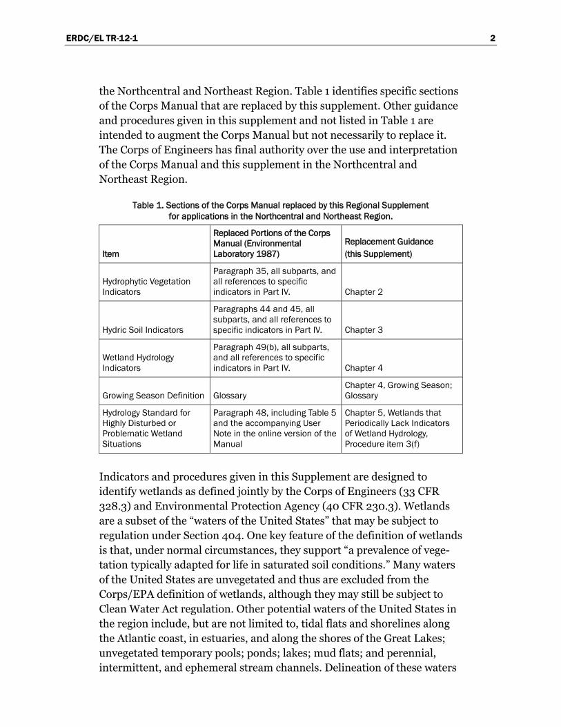
the Northcentral and Northeast Region. Table 1 identifies specific sections of the Corps Manual that are replaced by this supplement. Other guidance and procedures given in this supplement and not listed in Table 1 are intended to augment the Corps Manual but not necessarily to replace it. The Corps of Engineers has final authority over the use and interpretation of the Corps Manual and this supplement in the Northcentral and Northeast Region.
Table 1. Sections of the Corps Manual replaced by this Regional Supplement for applications in the Northcentral and Northeast Region.
Item
Replaced Portions of the Corps Manual (Environmental Laboratory 1987)
Replacement Guidance (this Supplement)
Hydrophytic Vegetation Indicators
Paragraph 35, all subparts, and all references to specific indicators in Part IV. Chapter 2
Hydric Soil Indicators
Paragraphs 44 and 45, all subparts, and all references to specific indicators in Part IV. Chapter 3
Wetland Hydrology Indicators
Paragraph 49(b), all subparts, and all references to specific indicators in Part IV. Chapter 4
Growing Season Definition Glossary Chapter 4, Growing Season; Glossary
Hydrology Standard for Highly Disturbed or Problematic Wetland Situations
Paragraph 48, including Table 5 and the accompanying User Note in the online version of the Manual
Chapter 5, Wetlands that Periodically Lack Indicators of Wetland Hydrology, Procedure item 3(f)
Indicators and procedures given in this Supplement are designed to identify wetlands as defined jointly by the Corps of Engineers (33 CFR 328.3) and Environmental Protection Agency (40 CFR 230.3). Wetlands are a subset of the “waters of the United States” that may be subject to regulation under Section 404. One key feature of the definition of wetlands is that, under normal circumstances, they support “a prevalence of vege-tation typically adapted for life in saturated soil conditions.” Many waters of the United States are unvegetated and thus are excluded from the Corps/EPA definition of wetlands, although they may still be subject to Clean Water Act regulation. Other potential waters of the United States in the region include, but are not limited to, tidal flats and shorelines along the Atlantic coast, in estuaries, and along the shores of the Great Lakes; unvegetated temporary pools; ponds; lakes; mud flats; and perennial, intermittent, and ephemeral stream channels. Delineation of these waters

ERDC/EL TR-12-1 3
is based on the high tide line, the “ordinary high water mark” (33 CFR 328.3e), or other criteria and is beyond the scope of this Regional Supplement.
Amendments to this document will be issued periodically in response to new scientific information and user comments. Between published ver-sions, Headquarters, U.S. Army Corps of Engineers may provide updates to this document and any other supplemental information used to make wetland determinations under Section 404 and Section 10. Wetland delin-eators should use the most recent approved versions of this document and supplemental information. See the Corps of Engineers Headquarters reg-ulatory web site for information and updates (http://www.usace.army.mil/-CECW/Pages/reg_supp.aspx). The Corps of Engineers has established an inter-agency National Advisory Team for Wetland Delineation. The Team’s role is to review new data and make recommendations for changes in wetland-delineation procedures to Headquarters, U.S. Army Corps of Engineers. Items for consideration should include full documentation and supporting data and should be submitted to:
National Advisory Team for Wetland Delineation Regulatory Branch (Attn: CECW-CO) U.S. Army Corps of Engineers 441 G Street, N.W. Washington, DC 20314-1000
Applicable region and subregions
This supplement is applicable to the Northcentral and Northeast Region, which consists of all or portions of 15 states: Connecticut, Illinois, Indiana, Maine, Massachusetts, Michigan, Minnesota, New Hampshire, New Jersey, New York, Ohio, Pennsylvania, Rhode Island, Vermont, and Wisconsin (Figure 1). The region encompasses considerable topographic and climatic diversity, but is differentiated from surrounding regions mainly by the combination of a humid temperate climate with cold, snowy winters, short growing seasons, and seasonally frozen soils in many areas; glacially sculpted landscape; hardwood, conifer, mixed-forest, and hard-wood-savanna natural vegetation; and the preponderance of forest, crop, pasture, and developed land uses (Bailey 1995, USDA Natural Resources Conservation Service 2006).
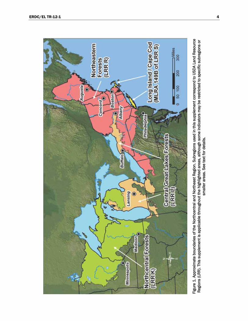
ERDC/EL TR-12-1 4
Figu
re 1
. App
roxi
mat
e bo
unda
ries
of th
e N
orth
cent
ral a
nd N
orth
east
Reg
ion.
Sub
regi
ons
used
in th
is s
uppl
emen
t cor
resp
ond
to U
SDA
Land
Res
ourc
e Re
gion
s (L
RR).
This
sup
plem
ent i
s ap
plic
able
thro
ugho
ut th
e hi
ghlig
hted
are
as, a
lthou
gh s
ome
indi
cato
rs m
ay b
e re
stric
ted
to s
peci
fic s
ubre
gion
s or
sm
alle
r are
as. S
ee te
xt fo
r det
ails
.
ERDC/EL TR-12-1 5
The approximate spatial extent of the Northcentral and Northeast Region is shown in Figure 1. The region map is based on a combination of Land Resource Regions (LRR) K, L, and R, and Major Land Resource Area (MLRA) 149B in LRR S, as recognized by the U.S. Department of Agri-culture (USDA Natural Resources Conservation Service 2006). Most of the wetland indicators presented in this supplement are applicable throughout the entire Northcentral and Northeast Region. However, some indicators are restricted to specific subregions (i.e., LRRs) or smaller areas (i.e., MLRAs).
Region and subregion boundaries are depicted in Figure 1 as sharp lines. However, climatic conditions and the physical and biological character-istics of landscapes do not change abruptly at the boundaries. In reality, regions and subregions often grade into one another in broad transition zones that may be tens or hundreds of miles wide. The lists of wetland indicators presented in these Regional Supplements may differ between adjoining regions or subregions. In transitional areas, the investigator must use experience and good judgment to select the supplement and indicators that are appropriate to the site based on its physical and bio-logical characteristics. Wetland boundaries are not likely to differ between two supplements in transitional areas, but one supplement may provide more detailed treatment of certain problem situations encountered on the site. If in doubt about which supplement to use in a transitional area, apply both supplements and compare the results. For additional guidance, contact the appropriate Corps of Engineers District Regulatory Office. Contact information for District regulatory offices is available at the Corps Headquarters web site (http://www.usace.army.mil/CECW/Pages/reg_districts.aspx).
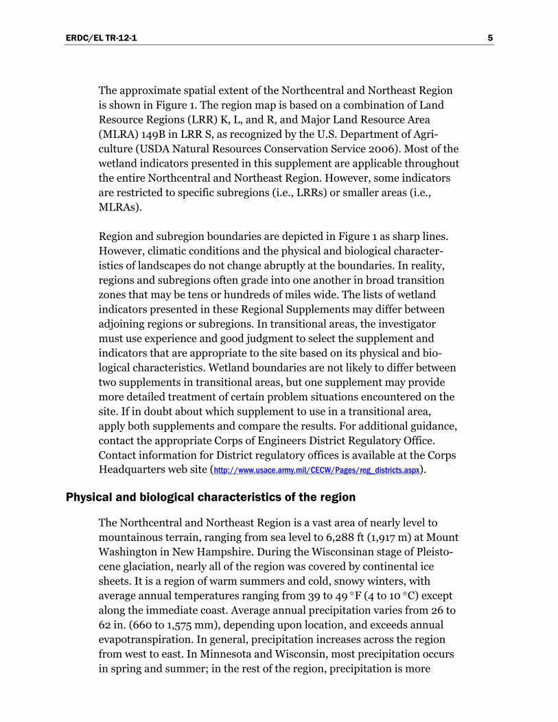
Physical and biological characteristics of the region
The Northcentral and Northeast Region is a vast area of nearly level to mountainous terrain, ranging from sea level to 6,288 ft (1,917 m) at Mount Washington in New Hampshire. During the Wisconsinan stage of Pleisto-cene glaciation, nearly all of the region was covered by continental ice sheets. It is a region of warm summers and cold, snowy winters, with average annual temperatures ranging from 39 to 49 °F (4 to 10 °C) except along the immediate coast. Average annual precipitation varies from 26 to 62 in. (660 to 1,575 mm), depending upon location, and exceeds annual evapotranspiration. In general, precipitation increases across the region from west to east. In Minnesota and Wisconsin, most precipitation occurs in spring and summer; in the rest of the region, precipitation is more
ERDC/EL TR-12-1 6
evenly distributed throughout the year (Bailey 1995, USDA Natural Resources Conservation Service 2006). The combination of relatively abundant rainfall, low evapotranspiration, and varied topography has created a region rich in perennial, intermittent, and ephemeral streams, natural lakes, and wetlands.
Soil parent materials in the Northcentral and Northeast Region are pre-dominantly the result of Pleistocene glaciations. Glaciers and meltwater shaped the landscape of the region and deposited the debris as glacial landforms, including moraines, drumlins, eskers, outwash plains, kettles, lake plains, deltas, and other features (Embleton and King 1968). Nearly every landscape in the region has been smoothed by glacial ice and has some sort of glacial material on its surface.
Glacial features can be categorized into two broad groups: ice-contact deposits and glaciofluvial or meltwater deposits. Till is the most extensive ice-contact deposit in the region. It is an unsorted mixture of fine particles, sand, gravel, cobbles, and boulders that was scoured and redeposited by ice (Embleton and King 1968). Deposits are generally thickest in valleys and thinnest over highlands. The properties of glacial till are directly related to the source materials. Till from granitic bedrock is commonly rocky, sandy, and acidic. Till from Mesozoic rocks can be reddish in color, and that derived from former lake plains can be very clayey. Ground moraine is a landform of low relief consisting of basal till deposited by receding ice. The topography is often gently rolling, with numerous shal-low depressions. Terminal and lateral moraines are ridges or chains of hills that formed at the ends and sides of glaciers, respectively. For exam-ple, Long Island in New York was formed, in part, by the terminal moraine marking the southernmost extent of Wisconsinan glaciers. Drumlins are elongated, streamlined hills of glacial till. They occur in groups oriented parallel to the direction of glacial flow and number in the thousands in some areas. Extensive drumlin fields are found in northwestern New York, east-central Wisconsin, and south-central New England. Slope wetlands are associated with drumlins and other ice-contact deposits throughout the region as a result of water perching in the spring over dense glacial till. Eskers are long narrow ridges composed of stratified sand and gravel deposited by streams flowing through tunnels within and beneath glaciers (Embleton and King 1968; Martini et al. 2001).
ERDC/EL TR-12-1 7
Glaciofluvial deposits are formed of materials transported by glacial melt-water. They tend to be sorted by particle size, forming stratified deposits. Meltwater emerging from beneath a glacier often forms braided streams that deposit sand and gravel over a broad area, producing an outwash plain. As glaciers recede, blocks of ice may be isolated and partly buried in the accumulating sediments. As these blocks melt, the unsupported glacial sediments collapse and form depressions called kettles (Embleton and King 1968). Walden Pond in Massachusetts is one example. Some outwash plains are dotted with numerous kettles and are known as pitted outwash. In the Northcentral and Northeast Region, numerous wetlands exist today where kettle holes intercept the regional water table. The finer particles in glacial meltwater may be deposited farther downstream and in the still waters of glacial lakes. Lake (lacustrine) deposits include horizontal strata of silts and clays that accumulate on lake bottoms, and deltas of sandy materials deposited at the mouths of incoming streams. Lacustrine deposits in some areas support complexes of small, rainwater-fed depressional wetlands (Stone and Ashley 1992). In other areas, such as in northern Minnesota, extensive organic soils have formed on glacial lake plains.
Post-glacial, clayey, marine deposits exist in the Champlain Valley of Vermont and along the Atlantic coast from southeastern Massachusetts north to Canada. In Maine, marine deposits occur at elevations up to 420 ft (128 m) above sea level, as a result of post-glacial isostatic (crustal) rebound (Maine Geological Survey 2005). These clayey deposits can be somewhat confusing for wetland delineation as they commonly have gray, lithochromic (inherited from parent material) colors. In addition, wind-blown deposits of silt and fine sand (loess) form a surface cap over glacial materials in some soils in the region. Other parent materials in the region include sand dunes adjacent to the Great Lakes and the Atlantic coast, and recent alluvial deposits along the Mississippi, Hudson, Connecticut, and other rivers.
The Northcentral and Northeast Region occupies the transition zone between the boreal forest to the north and broadleaf deciduous forest to the south. Individual forest stands may consist primarily of conifers, hard-woods, or a mixture of the two. Pines (Pinus spp.) and other conifers often dominate in areas with nutrient-poor soils or recent disturbance by fire or human activity. Areas with nutrient-rich soils are often dominated by hardwoods, such as sugar maple (Acer saccharum), American basswood (Tilia americana), and American beech (Fagus grandifolia) (Bailey 1995).
ERDC/EL TR-12-1 8
In the mountainous areas of New York and the New England states, there is distinct altitudinal zonation of forest types.
The Northcentral and Northeast Region is composed of three major sub-regions: Northcentral Forests (corresponds to LRR K), Central Great Lakes Forests (LRR L), and Northeastern Forests (LRR R). In addition, the Long Island/Cape Cod area (MLRA 149B in LRR S) has been included in this region because of its similar climate, geologic history, and soil parent materials (Figure 1). Important characteristics of each subregion are described briefly below; further details can be found in USDA Natural Resources Conservation Service (2006). Wetland indicators presented in this Regional Supplement are applicable across all subregions unless otherwise noted.
Northcentral Forests (LRR K)
This subregion lies mainly south and west of the western Great Lakes in Minnesota, Wisconsin, Michigan, and Illinois (Figure 1) and is covered mostly by level to gently rolling deposits of glacial till, loess, outwash, and glacial lake sediments. The subregion receives 26 to 34 in. (660 to 865 mm) of precipitation each year. The area is largely forested, with lesser amounts of cropland, grassland, and urban development. Common tree species in higher landscape positions include eastern white pine (Pinus strobus), red pine (P. resinosa), jack pine (P. banksiana), eastern hemlock (Tsuga canadensis), American beech, yellow birch (Betula alleghaniensis), paper birch (B. papyrifera), northern red oak (Quercus rubra), white oak (Q. alba), sugar maple, white ash (Fraxinus ameri-cana), and quaking aspen (Populus tremuloides). Lowlands are dominated mainly by black spruce (Picea mariana), tamarack (Larix laricina), nor-thern white cedar or arborvitae (Thuja occidentalis), balsam fir (Abies balsamea), black ash (Fraxinus nigra), green ash (F. pennsylvanica), silver maple (Acer saccharinum), red maple (A. rubrum), American elm (Ulmus americana), and swamp white oak (Q. bicolor) (USDA Natural Resources Conservation Service 2006).
Central Great Lakes Forests (LRR L)
This subregion contains most of Lower Michigan along with portions of Illinois, Indiana, Ohio, Pennsylvania, and New York (Figure 1). It consists of nearly level to gently rolling glacial plains covered by till, outwash, and glacial lake sediments with scattered moraine hills. Most of the area
ERDC/EL TR-12-1 9
receives 30 to 41 in. (760 to 1,040 mm) of precipitation each year, with higher amounts in the small area southeast of Lake Erie. The subregion supports mainly broadleaf deciduous forests dominated by bitternut hickory (Carya cordiformis), shagbark hickory (C. ovata), white oak, northern red oak, black oak (Quercus velutina), sugar maple, red maple, American beech, American elm, and American basswood. Eastern white pine, red pine, and jack pine are common species in the portion of the subregion in northwestern Lower Michigan (USDA Natural Resources Conservation Service 2006).
Northeastern Forests (LRR R)
This large subregion extends from northern Ohio to New Jersey to Maine (Figure 1) and encompasses a variety of landforms, including rugged mountains and highly dissected plateaus and plains. Most of the area is covered by a mantle of glacial till, outwash sands and gravels, and glacial lake sediments. Eskers, kames, and drumlins are common features in some areas. Deposits of recent alluvium are present along major rivers, and marine sediments are common along the coast and in the lower por-tions of river valleys. In the mountains, some areas are dominated by talus and exposed igneous and metamorphic bedrock. Average annual precipi-tation mostly ranges from 34 to 62 in. (865 to 1,575 mm), but is more than 100 in. (2,540 mm) on the highest peaks in Vermont and New Hampshire, and in the area of lake-effect snows east of Lake Ontario. The subregion supports a mosaic of northern hardwood, spruce, fir, and pine forests. Common species include American beech, paper birch, yellow birch, sugar maple, oaks, eastern hemlock, balsam fir, red spruce (Picea rubens), black spruce, eastern white pine, and quaking aspen (USDA Natural Resources Conservation Service 2006).
Long Island/Cape Cod (MLRA 149B)
This area is restricted to New York, Massachusetts, and Rhode Island and is part of LRR S, but is included in the Northcentral and Northeast Region (Figure 1). The area is formed of deep glacial outwash deposits of sand and gravel, mostly covered by a layer of glacial till. Moraines form scattered low hills and ridges. The area receives 41 to 48 in. (1,040 to 1,220 mm) of precipitation each year. Much of the area is developed. Native forests support pitch pine (Pinus rigida), eastern white pine, northern red oak, red maple, American beech, yellow birch, and other tree species (USDA Natural Resources Conservation Service 2006).
ERDC/EL TR-12-1 10
Types and distribution of wetlands
The Northcentral and Northeast Region is rich in wetlands, due in large part to plentiful precipitation, low evapotranspiration, and diverse land-scapes resulting from its recent glacial history. Some of the places where wetlands have formed include (1) shores of the region’s many lakes and ponds, (2) broad flats on former glacial lake plains, (3) kettle depressions where ice blocks were left on the landscape as the glaciers retreated, (4) depressions and blocked drainages formed by morainal deposits, (5) outwash deposits of sand and gravel where groundwater discharges or is often near the surface, and (6) deposits of unsorted glacial till that have created relatively impermeable subsoils on flats and slopes. The region also contains large river systems that periodically flood low-lying areas, creating floodplain wetlands of various types. Coastal marshes and dune/swale wetlands have also formed along the Atlantic coast, in estu-aries, and along the shores of the Great Lakes. Generalized descriptions of the region’s wetlands can be found in Curtis (1971), Eggers and Reed (1997), and Tiner (2005). Additional details on wetland plant communities are given in state natural heritage program reports (e.g., Reschke 1990, Minnesota Department of Natural Resources 2003, and Sperduto 2005) and National Wetlands Inventory (NWI) state reports for Rhode Island and Connecticut (Tiner 1989; Metzler and Tiner 1992). Specific wetland types are described by Johnson (1985), Wright et al. (1992), Tiner (2008), and many others.
Wetlands in the region can be divided broadly into freshwater and salt-water wetlands. Most saltwater wetlands in the region are dominated by herbaceous emergent plants. Freshwater wetlands, on the other hand, can be categorized as forested, shrub-dominated, or herbaceous, and further subdivided by soil type (e.g., mineral or organic) and hydrology. For example, various types of bogs are common in the region. Bogs are peat-forming wetlands with acidic soils that support relatively few species of acid-loving plants, such as Sphagnum mosses, and develop in areas where precipitation is the primary water source. Other peat-forming wetlands, called fens, have circumneutral to alkaline soils that range from mineral-poor to mineral-rich. Their hydrology is driven predominantly by ground-water discharge and their plant communities can be very diverse.
Forested wetlands are the most abundant wetlands in the region and represent many different types. Boreal coniferous forested wetlands occur in the more northerly parts of the region and at higher elevations in more
ERDC/EL TR-12-1 11
southerly areas. They may support black spruce, tamarack, balsam fir, northern white cedar, Atlantic white cedar (Chamaecyparis thyoides), or red spruce. Coniferous forested bogs include tamarack and black spruce bogs, and usually have a continuous carpet of Sphagnum. Those forming on neutral to alkaline peat soils, such as northern white cedar swamps, lack the carpet of Sphagnum but may have a rich understory of other bryo-phytes. Forested fens with similar mineral-rich peat soils often support northern white cedar and tamarack. Eastern hemlock, eastern white pine, and pitch pine also dominate coniferous forested wetlands in various parts of the region.
Deciduous forested wetlands are common throughout much of the region in depressions, on floodplains, on flats on glacial lake plains, and along lake shores. Dominant swamp trees include red maple, black ash, green ash, and pin oak (Quercus palustris). Skunk cabbage (Symplocarpus foetidus), several species of ferns (e.g., cinnamon [Osmunda cinna-momea], royal [O. regalis], sensitive [Onoclea sensibilis], and eastern marsh fern [Thelypteris palustris]), and numerous shrubs (e.g., highbush blueberry [Vaccinium corymbosum], alders [Alnus spp.], arrowwood [Viburnum dentatum], withe-rod [V. nudum var. cassinoides], red-osier dogwood [Cornus sericea = C. stolonifera] and silky dogwood [C. amomum]) are common in many swamps. Floodplain forests occupy low-lands adjacent to the larger rivers in the region. Silver maple, eastern cottonwood (Populus deltoides), American sycamore (Platanus occi-dentalis), American elm, black willow (Salix nigra), and balsam poplar (Populus balsamifera) are characteristic bottomland trees, while ostrich fern (Matteuccia struthiopteris), false nettle (Boehmeria cylindrica), and Canadian woodnettle (Laportea canadensis) are common herbs. Other important wetland trees include yellow birch, black gum (Nyssa syl-vatica), swamp white oak, and quaking aspen. Wet flatwoods occur on broad, glacial lake plains, such as those along Lake Ontario. These wet-lands are dominated by typical swamp species, but are not flooded as long as most swamps. Instead, they have seasonally high or perched water tables that may persist from winter to early summer.
Shrub bogs are prominent in northern areas, while deciduous shrub swamps are common throughout the region. Typical shrub-bog species that grow on acidic peat soils in association with a mat of Sphagnum mosses include evergreen members of the heath family, such as leatherleaf (Chamaedaphne calyculata), bog laurel (Kalmia polifolia), bog rosemary
ERDC/EL TR-12-1 12
(Andromeda polifolia var. glaucophylla = A. glaucophylla), Labrador tea (Ledum groenlandicum), and cranberries (Vaccinium macrocarpon and V. oxycoccos), as well as sweetgale (Myrica gale), black spruce, tamarack, purple pitcher plant (Sarracenia purpurea), sundews (Drosera spp.), bog aster (Oclemena nemoralis = Aster nemoralis), bog goldenrod (Solidago uliginosa), and threeleaf false lily-of-the-valley (Maianthemum trifolium = Smilacina trifolia). Characteristic species of deciduous shrub swamps are alders (Alnus incana and A. serrulata), willows (Salix spp.), dog-woods, swamp rose (Rosa palustris), steeplebush (Spiraea tomentosa), white meadowsweet (Spiraea alba), and buttonbush (Cephalanthus occi-dentalis). The ground layer can be composed of a diversity of ferns, sedges, rushes, and forbs, such as those listed below in the paragraph describing wet meadows. The ground layer in disturbed, deciduous shrub swamps may be composed of reed canarygrass (Phalaris arundinacea) or other invasive species.
Herbaceous wetlands include marshes, wet meadows, and fens. Two basic types of marshes are found in the region – freshwater and saline marshes. The former occur throughout the region in lakes, ponds, shallow slow-flowing rivers, and isolated depressions, while the latter are found in the intertidal zone of estuaries.
Freshwater marshes, both tidal and nontidal, are generally represented by cattails (Typha latifolia and T. angustifolia), pickerelweed (Pontederia cordata), arrowheads (Sagittaria spp.), yellow pond-lily (Nuphar lutea), white waterlily (Nymphaea odorata), softstem bulrush (Schoenoplectus tabernaemontani = Scirpus validus), bur-reeds (Sparganium spp.), and wild rice (Zizania aquatica and Z. palustris). Bayonet rush (Juncus militaris) grows in shallow water along sandy lake shores. Common reed (Phragmites australis) dominates many disturbed freshwater and brackish marshes.
Salt and brackish marshes are dominated by halophytes or salt-tolerant species. Smooth cordgrass (Spartina alterniflora) occupies the low marsh that is flooded at least daily by the tides. The high marsh is more diverse, with saltmeadow cordgrass (Spartina patens), salt grass (Distichlis spicata), and black grass (Juncus gerardii) being most common, while switch grass (Panicum virgatum) and the shrubby marsh-elder (Iva frutescens) often form the marsh border. Other species characteristic of salt marshes include seaside goldenrod (Solidago sempervirens), salt-
ERDC/EL TR-12-1 13
marsh aster (Symphyotrichum tenuifolium = Aster tenuifolius), saltmarsh bulrush (Schoenoplectus robustus = Scirpus robustus), and rose mallow (Hibiscus moscheutos); these species become more abundant and domi-nate brackish marshes upstream.
Herbaceous fens occur in northern portions of the region and elsewhere at higher altitudes where they are less common. Fen species at the most mineral-rich end of the gradient include many calciphiles that thrive in soils with higher pH. They include numerous herbs, such as marsh muhly (Muhlenbergia glomerata), bluejoint grass (Calamagrostis canadensis), twig rush (Cladium mariscoides), several sedges (Carex flava, C. sterilis, C. lasiocarpa, C. lacustris, C. stricta, and C. utriculata), thinleaf cotton-sedge (Eriophorum viridicarinatum), moor rush (Juncus stygius), grass-of-Parnassus (Parnassia glauca), purple avens (Geum rivale), white lady’s slipper (Cypripedium candidum), and marsh cinquefoil (Comarum palustre = Potentilla palustris), plus several shrubs including shrubby cinquefoil (Dasiphora fruticosa ssp. floribunda = Potentilla fruticosa), alderleaf buckthorn (Rhamnus alnifolia), sageleaf willow (Salix candida), autumn willow (S. serissima), bog birch (Betula pumila), sweetgale, speckled alder (Alnus incana), and red-osier dogwood. Minerotrophic moss species (e.g., Drapanocladus aduncus and Campylium stellatum) may or may not be present.
Wet meadows occur on seasonally saturated mineral or organic soils that may be associated with high water tables and/or surface water inputs. They may be characterized by (1) a single species, such as reed canary-grass, bluejoint grass, or sweetflag (Acorus calamus); (2) various sedges, such as tussock sedge (Carex stricta), lake sedge (C. lacustris), green bulrush (Scirpus atrovirens), and woolgrass (Scirpus cyperinus), that can be described as a sedge-meadow subtype; or (3) a diverse assemblage of plants including many flowering herbs. Among the more common flower-ing herbs are Joe-Pye-weeds (Eupatoriadelphus spp.), boneset (Eupa-torium perfoliatum), square-stem monkeyflower (Mimulus ringens), asters (e.g., Symphyotrichum puniceum [= Aster puniceus], S. lateri-florum, S. lanceolatum, S. novi-belgii, Doellingeria umbellata [= Aster umbellatus]), goldenrods (Euthamia spp. and Solidago spp.), fringed loosestrife (Lysimachia ciliata), swamp candles (L. terrestris), irises (Iris spp.), jewelweed (Impatiens capensis and I. pallida), beggar-ticks (Bidens spp.), swamp milkweed (Asclepias incarnata), blue vervain (Verbena hastata), ironweeds (Vernonia spp.), and willow-herbs (Epilo-
ERDC/EL TR-12-1 14
bium spp.). Many wet meadows occur in agricultural areas where they are often used as pasture.
Many wetlands are used for agricultural purposes, including commercial cranberry bogs, farmed mucklands, wild rice impoundments, farmed floodplains, and sod fields. Commercial cranberry bogs generally were constructed from existing wetlands but, more recently, have been created in sandy uplands by excavating to a depth where the water table is at or near the surface for extended periods. These bogs are diked and water levels controlled by irrigation or dewatering. Farmed mucklands were created from hardwood swamps, tamarack swamps, and sedge meadows. After removing natural vegetation, diking, and draining through the use of pumps and siphons, their productive organic soils are planted with a vari-ety of crops including onions, lettuce, celery, and carrots. In Minnesota, wetlands have been converted to impoundments for cultivating wild rice (Zizania palustris). Many floodplains in the region have been converted to row crops (e.g., corn or soybeans) and some of these are flooded often enough and long enough to meet wetland standards. Sod fields managed to produce lawn or turf grasses, predominantly Kentucky bluegrass (Poa pratensis), are often constructed in wetlands where the surface water is drained by ditches and groundwater levels are closely managed.
Numerous nonnative and/or invasive species have replaced native species and reduced plant diversity in one or more wetland types in the region. Among the problematic herbs are common reed, reed canarygrass, cattails (e.g., Typha × glauca), purple loosestrife (Lythrum salicaria), Japanese stiltgrass (Microstegium vimineum = Eulalia viminea), garlic mustard (Alliaria petiolata), and Japanese knotweed (Fallopia japonica = Polygonum cuspidatum) plus three aquatic species – water chestnut (Trapa natans), curly pondweed (Potamogeton crispus), and Eurasian watermilfoil (Myriophyllum spicatum). Major invasive woody plants include common buckthorn (Rhamnus cathartica), glossy buckthorn (Frangula alnus = Rhamnus frangula), multiflora rose (Rosa multiflora), non-native honeysuckles (Lonicera spp.), and Japanese barberry (Berberis thunbergii).
ERDC/EL TR-12-1 15
2 Hydrophytic Vegetation Indicators Introduction
The Corps Manual defines hydrophytic vegetation as the community of macrophytes that occurs in areas where inundation or soil saturation is either permanent or of sufficient frequency and duration to influence plant occurrence. The manual uses a plant-community approach to evaluate vegetation. Hydrophytic vegetation decisions are based on the assemblage of plant species growing on a site, rather than the presence or absence of particular indicator species. Hydrophytic vegetation is present when the plant community is dominated by species that require or can tolerate prolonged inundation or soil saturation during the growing season. Hydrophytic vegetation in the Northcentral and Northeast Region is identified by using the indicators described in this chapter.
Many factors besides site wetness affect the composition of the plant community in an area, including regional climate, local weather patterns, topography, soils, natural and human-caused disturbances, and current and historical plant distributional patterns at various spatial scales. Braun (1950) described the vegetation of this region as “… a complex vegetation unit most conspicuously characterized by the prevalence of the deciduous habit of most of its woody constituents. This gives to it a certain uniformity of physiognomy, with alternating summer green and winter leafless aspects. Evergreen species, both broad-leaved and needle-leaved, occur in the arboreal and shrub layers, particularly in seral stages and in marginal and transitional areas.” The vegetation reflects the region’s glacial past and the most recent retreat of continental glaciers about 10,000 years ago. Freshly exposed tills and bedrock areas were originally dominated by boreal coniferous forest (Davis 1981), which was later replaced mostly by deciduous forests from the west and south of the region and by prairies penetrating eastward (Barbour and Billings 1988). The migration of past and present vegetation across this topographically and climatically varied region has resulted in a highly diverse flora. The regional flora contains more than 4,000 vascular plant species (Stein et al. 2000), of which approximately 2,800 species occur in wetlands to some degree (Reed 1988).
Human disturbances and land-use patterns have affected some parts of the region more than others. Prior to European settlement, Native Ameri-
ERDC/EL TR-12-1 16
cans used fire to clear underbrush in forested areas and woody vegetation from grasslands, but their activities had little long-lasting impact (Russell 1983). Greater impacts occurred in the 1800s due to extensive logging for pine and hemlock, clearing of forests for homesteading and grazing, and the beginning of a long-term trend in conversion of forest to agriculture and urban development. These major land-use changes have increased the number and occurrence of “weedy” species in the flora. More than 30 per-cent of the flora in many parts of the region now consists of non-native species (Stuckey and Barkley 1993).
The characteristics of wetland plant communities in the region are also affected by seasonal changes in availability of water, short- and long-term droughts, and natural and human-caused disturbances (e.g., floods, fires, grazing). Wetlands subject to seasonal hydrology in the region include wet meadows, springs, seeps, seasonal ponds, vernal pools, and floodplain forested wetlands. These wetlands often exhibit seasonal shifts in vege-tation composition, potentially changing the status of the community from hydrophytic during the wet season to non-hydrophytic during the dry sea-son. Long-term climatic fluctuations (e.g., multi-year droughts) and fluc-tuations in lake and sea levels can also change the composition of plant communities over longer periods (Barkley 1986). Woody shrubs and trees in wetlands are often resistant to droughts, while herbaceous vegetation may show dramatic turnover in species composition from drought years to pluvial years. See Chapter 5 for discussions of these and other problematic vegetation situations in the region.
Hydrophytic vegetation decisions are based on the wetland indicator status (Reed [1988] or current approved list) of species that make up the plant community. Species in the facultative categories (FACW, FAC, and FACU) are recognized as occurring in both wetlands and uplands to vary-ing degrees. Although most wetlands are dominated mainly by species rated OBL, FACW, and FAC, some wetland communities may be domi-nated primarily by FACU species and cannot be identified by dominant species alone. In those cases, other indicators of hydrophytic vegetation must also be considered, particularly where indicators of hydric soils and wetland hydrology are present. This situation is not necessarily due to inaccurate wetland indicator ratings; rather, it is due to the broad toler-ances of certain plant species that allow them to be widely distributed across the moisture gradient. Therefore, for some species, it is difficult to
ERDC/EL TR-12-1 17
assign a single indicator status rating that encompasses all of the various landscape and ecological settings it can occupy.
Hydrophytic vegetation indicators and procedures presented in this chap-ter are designed to identify the majority of wetland plant communities in the region. However, some wetland communities may lack any of these indicators. These situations are considered in Chapter 5 (Difficult Wetland Situations in the Northcentral and Northeast Region).
Guidance on vegetation sampling and analysis
General guidance on sampling of vegetation for wetland-delineation pur-poses is given in the Corps Manual. Those procedures are intended to be flexible and may need to be modified for application in a given region or on a particular site. Vegetation sampling done as part of a routine wetland delineation is designed to characterize the site in question rapidly. A balance must be established between the need to accomplish the work quickly and the need to characterize the site’s heterogeneity accurately and at an appropriate scale. The following guidance on vegetation sampling is intended to supplement the Corps Manual for applications in the Northcentral and Northeast Region.
The first step is to identify the major landscape or vegetation units so that they can be evaluated separately. This may be done in advance using an aerial photograph or topographic map, or by walking the site. In general, routine wetland determinations are based on visual estimates of percent cover of plant species that can be made either (1) within the vegetation unit as a whole, or (2) within one or more sampling plots established in representative locations within each unit. Percent cover estimates are more accurate and repeatable if taken within a defined plot. This also facilitates field verification of another delineator’s work. The sizes and shapes of plots, if used, may be modified as appropriate to adapt to site conditions and should be recorded on the field data form. When sampling near a plant community boundary, and particularly near the wetland boundary, it may be necessary to adjust plot size or shape to avoid over-lapping the boundary and extending into an adjacent community having different vegetation, soils, or hydrologic conditions.
If it is not possible to locate one or a few plots in a way that adequately represents the vegetation unit being sampled, then percent cover estimates for each species can be made during a meandering survey of the broader
ERDC/EL TR-12-1 18
community. If additional quantification of cover estimates is needed, then the optional procedure for point-intercept sampling along transects (see Appendix B) or other sampling procedures may be used to characterize the vegetation unit. To use either of these sampling methods, soil and hydro-logic conditions must be uniform across the sampled area.
Definitions of strata
Vegetation strata within the sampled area or plot are sampled separately when evaluating indicators of hydrophytic vegetation. In this region, the vegetation strata described in the Corps Manual are recommended (see below). Unless otherwise noted, a stratum for sampling purposes is defined as having 5 percent or more total plant cover. If a stratum has less than 5 percent cover during the peak of the growing season, then those species and their cover values should be recorded on the data form but should not be used in the calculations for the dominance test, unless it is the only stratum present.
1. Tree stratum – Consists of woody plants 3 in. (7.6 cm) or more in diameter at breast height (DBH), regardless of height.
2. Sapling/shrub stratum – Consists of woody plants less than 3 in. DBH and greater than or equal to 3.28 ft (1 m) tall.
3. Herb stratum – Consists of all herbaceous (non-woody) plants, including herbaceous vines, regardless of size, and woody plants less than 3.28 ft tall.
4. Woody vines – Consists of all woody vines greater than 3.28 ft in height.
Plot and sample sizes
Hydrophytic vegetation determinations under the Corps Manual are based on samples taken in representative locations within each community. Ran-dom sampling of the vegetation is not required, except for certain sampling approaches in comprehensive determinations or in rare cases where representative sampling might give misleading results. For routine determinations in fairly uniform vegetation, one or more plots in each community are usually sufficient for an accurate determination. Sampling of a multi-layered community is usually accomplished using a graduated series of plots, one for each stratum, or a number of small plots nested within the largest plot (Figure 2). Nested plots to sample the herb stratum can be helpful in forested areas with highly variable understories or in very diverse communities. Plant abundance data are averaged across the multiple small plots.
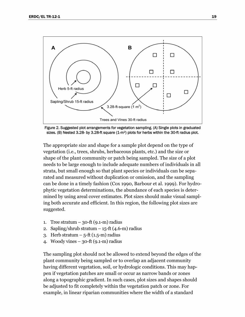
ERDC/EL TR-12-1 19
Figure 2. Suggested plot arrangements for vegetation sampling. (A) Single plots in graduated
sizes. (B) Nested 3.28- by 3.28-ft square (1-m2) plots for herbs within the 30-ft radius plot.
The appropriate size and shape for a sample plot depend on the type of vegetation (i.e., trees, shrubs, herbaceous plants, etc.) and the size or shape of the plant community or patch being sampled. The size of a plot needs to be large enough to include adequate numbers of individuals in all strata, but small enough so that plant species or individuals can be sepa-rated and measured without duplication or omission, and the sampling can be done in a timely fashion (Cox 1990, Barbour et al. 1999). For hydro-phytic vegetation determinations, the abundance of each species is deter-mined by using areal cover estimates. Plot sizes should make visual sampl-ing both accurate and efficient. In this region, the following plot sizes are suggested.
1. Tree stratum – 30-ft (9.1-m) radius 2. Sapling/shrub stratum – 15-ft (4.6-m) radius 3. Herb stratum – 5-ft (1.5-m) radius 4. Woody vines – 30-ft (9.1-m) radius
The sampling plot should not be allowed to extend beyond the edges of the plant community being sampled or to overlap an adjacent community having different vegetation, soil, or hydrologic conditions. This may hap-pen if vegetation patches are small or occur as narrow bands or zones along a topographic gradient. In such cases, plot sizes and shapes should be adjusted to fit completely within the vegetation patch or zone. For example, in linear riparian communities where the width of a standard
ERDC/EL TR-12-1 20
plot may exceed the width of the plant community, an elongated rectang-ular plot or belt transect that follows the stream is recommended. If possible, the area sampled should be equivalent to the 30-ft-radius plot (2,827 ft2 [263 m2]) for the tree stratum or the 15-ft-radius plot (707 ft2 [65.7 m2]) for the sapling/shrub stratum. Thus the sapling/shrub stratum could be sampled using a 10- by 71-ft (3.1- by 21.6-m) plot lying completely within the riparian fringe. An alternative approach involves sampling a series of small subplots (e.g., 5 by 5 ft [1.5 by 1.5 m], or 10 by 10 ft [3.1 by 3.1 m]) in the riparian community and averaging the data across subplots.
A 30-ft radius tree plot works well in most forests but can be increased to 35 ft (10.7 m) or 40 ft (12.2 m) or more in a nonlinear forest stand if tree diversity is high or diameters are large. Highly diverse or patchy commun-ities of herbs or other low vegetation may be sampled with nested 3.28- by 3.28-ft (1-m2) quadrats randomly located within a 30-ft radius (Figure 2B). Furthermore, point-intercept sampling performed along a transect is an alternative to plot-based methods that can improve the accuracy and repeatability of vegetation sampling in diverse or heterogeneous communities (see Appendix B). To use this method, soil and hydrologic conditions must be uniform across the area where transects are located.
Vegetation sampling guidance presented here should be adequate for hydrophytic vegetation determinations in most situations. However, many variations in vegetation structure, diversity, and spatial arrangement exist on the landscape that are not addressed in this supplement. A list of references is given in Table 2 for more complex sampling situations. If alternative sampling techniques are used, they should be derived from the scientific literature and described in field notes or in the delineation report. The basic data must include abundance values for each species present. Typical abundance measures include basal area for tree species, percent areal cover, stem density, or frequency based on point-intercept sampling. In any case, the data must be in a format that can be used in the dominance test or prevalence index for hydrophytic vegetation (see the section on Hydrophytic Vegetation Indicators).
In this supplement, absolute percent cover is the preferred abundance measure for all species. For percent cover estimates, plants do not need to be rooted in the plot as long as they are growing under the same soil and hydrologic conditions. It may be necessary to exclude plants that overhang the plot if they are rooted in areas having different soil and hydrologic conditions, particularly when sampling near the wetland boundary.
ERDC/EL TR-12-1 21
Table 2. Selected references to additional vegetation sampling approaches that could be used in wetland delineation.
Reference Comment
Brohman, R. J., and L. D. Bryant, eds. 2005. Existing vegetation classification and mapping technical guide, Version 1.0. General Technical Report WO-67. Washington, DC: U.S. Department of Agriculture Forest Service.
Contains a brief summary of vegetation sampling methods.
Kent, M., and P. Coker. 1992. Vegetation description and analysis: A practical approach. New York, NY: Wiley.
Contains simple and clear methods for setting up a study and collecting and analyzing the data. Initial chapters are helpful for data collection and sampling approaches in wetland delineation.
Mueller-Dombois, D., and H. Ellenberg. 1974. Aims and methods of vegetation ecology. New York, NY: Wiley.
A standard text in vegetation ecology, sampling, and analysis. This reference provides many sampling and analytical methods that are helpful in complex delineations.
Tiner, R. W. 1999. Wetland indicators: A guide to wetland delineation, classification, and mapping. Boca Raton, FL: CRC Press.
Includes reviews of various sampling techniques and provides a list of vegetation references.
U.S. Department of the Interior (USDI), Bureau of Land Management. 1996. Sampling vegetation attributes. BLM/RS/ST-96/002+1730. Denver, CO.
Describes many aspects of vegetation sampling, including sampling protocols, data collection, and analysis.
Basal area is an alternative abundance measure for species in the tree stratum. Basal area of each species in a stand can be estimated quickly and efficiently with a basal-area prism or angle gauge. In this region, a prism with a basal-area factor (BAF) of 10 works well. Basal-area estimates can be used to select dominant species from the tree stratum for use in the dominance test for hydrophytic vegetation (see Hydrophytic Vegetation Indicators). However, basal-area estimates cannot be used to calculate a prevalence index, which is based on absolute percent cover of species in each stratum. Therefore, if basal-area estimates are used initially to eval-uate the tree stratum but the dominance test is inconclusive, then the use of the prevalence index will require that the tree stratum be resampled to estimate absolute percent cover of each species.
Seasonal considerations and cautions
To the extent possible, the hydrophytic vegetation decision should be based on the plant community that is normally present during the wet portion of the growing season in a normal rainfall year. However, wetland determinations must often be performed at other times of year, or in years with unusual or atypical weather conditions. The Northcentral and North-east Region has a temperate climate with cold, snowy winters. Vegetation
ERDC/EL TR-12-1 22
sampling for a wetland determination can be challenging when some plants are covered by snow or die back due to freezing temperatures or other factors. At these times, experience and professional judgment may be required to adapt the vegetation sampling scheme or use other sources of information to determine the plant community that is normally present.
When an on-site evaluation of the vegetation is impractical due to snow and ice or other factors, one option is to use existing off-site data sources, such as National Wetlands Inventory (NWI) maps, soil surveys, and aerial photographs, to make a preliminary hydrophytic vegetation determina-tion. These sources may be supplemented with limited on-site data, including those plant species that can be observed and identified. Later, when conditions are favorable, an on-site investigation should be made to verify the preliminary determination and complete the wetland delineation.
Other factors can alter the plant community on a site and affect a hydro-phytic vegetation determination, including seasonal changes in species composition, intensive grazing, wildfires and other natural disturbances, and human land-use practices. These factors are considered in Chapter 5.
Hydrophytic vegetation indicators
The following indicators should be applied in the sequence presented. The stepwise procedure is designed to reduce field effort by requiring that only one or two indicators — variations of the dominance test — be evaluated in the majority of wetland determinations. However, hydrophytic vegetation is present if any of the indicators is satisfied. All of these indicators are applicable throughout the entire Northcentral and Northeast Region.
Indicators of hydrophytic vegetation involve looking up the wetland indi-cator status of plant species on the wetland plant list (Reed [1988] or current list). For the purposes of this supplement, only the five basic levels of wetland indicator status (i.e., OBL, FACW, FAC, FACU, and UPL) are used in hydrophytic vegetation indicators. Plus (+) and minus (–) modifiers are not used (e.g., FAC–, FAC, and FAC+ plants are all considered to be FAC). For species listed as NI (reviewed but given no regional indicator) or NO (no known occurrence in the region at the time the list was compiled), apply the indicator status assigned to the species in the nearest adjacent region. If the species is listed as NI or NO but no adjacent regional indicator is assigned, do not use the species to calculate hydrophytic vegetation
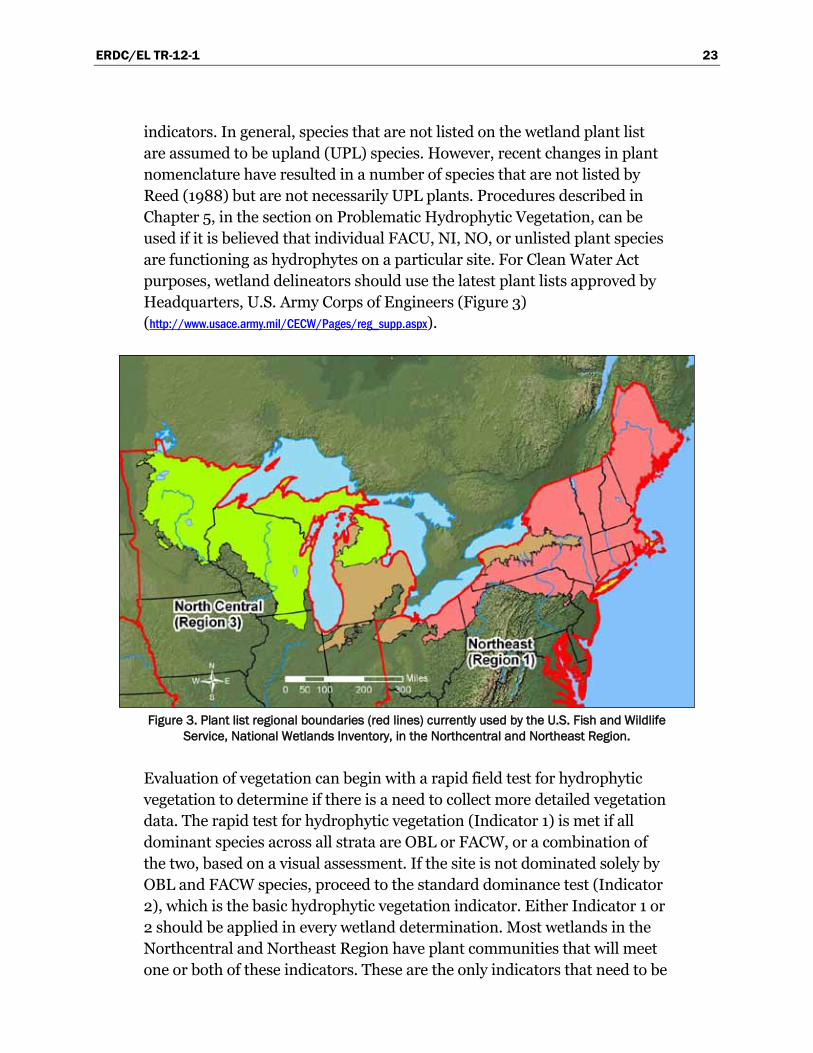
ERDC/EL TR-12-1 23
indicators. In general, species that are not listed on the wetland plant list are assumed to be upland (UPL) species. However, recent changes in plant nomenclature have resulted in a number of species that are not listed by Reed (1988) but are not necessarily UPL plants. Procedures described in Chapter 5, in the section on Problematic Hydrophytic Vegetation, can be used if it is believed that individual FACU, NI, NO, or unlisted plant species are functioning as hydrophytes on a particular site. For Clean Water Act purposes, wetland delineators should use the latest plant lists approved by Headquarters, U.S. Army Corps of Engineers (Figure 3) (http://www.usace.army.mil/CECW/Pages/reg_supp.aspx).
Figure 3. Plant list regional boundaries (red lines) currently used by the U.S. Fish and Wildlife
Service, National Wetlands Inventory, in the Northcentral and Northeast Region.
Evaluation of vegetation can begin with a rapid field test for hydrophytic vegetation to determine if there is a need to collect more detailed vegetation data. The rapid test for hydrophytic vegetation (Indicator 1) is met if all dominant species across all strata are OBL or FACW, or a combination of the two, based on a visual assessment. If the site is not dominated solely by OBL and FACW species, proceed to the standard dominance test (Indicator 2), which is the basic hydrophytic vegetation indicator. Either Indicator 1 or 2 should be applied in every wetland determination. Most wetlands in the Northcentral and Northeast Region have plant communities that will meet one or both of these indicators. These are the only indicators that need to be
ERDC/EL TR-12-1 24
considered in most situations. However, some wetland plant communities may fail a test based only on dominant species. Therefore, in those cases where indicators of hydric soil and wetland hydrology are present, the vegetation should be re-evaluated with the prevalence index (Indicator 3), which takes non-dominant plant species into consideration, or by observing plant morphological adaptations for life in wetlands (Indicator 4). Finally, certain disturbed or problematic wetland situations may lack any of these indicators and are described in Chapter 5.
Procedure
The procedure for using hydrophytic vegetation indicators is as follows:
1. Apply Indicator 1 (Rapid Test for Hydrophytic Vegetation). a. If the plant community passes the rapid test for hydrophytic vegetation,
then the vegetation is hydrophytic and no further vegetation analysis is required.
b. If the rapid test for hydrophytic vegetation is not met, then proceed to step 2.
2. Apply Indicator 2 (Dominance Test). a. If the plant community passes the dominance test, then the vegetation
is hydrophytic and no further vegetation analysis is required. b. If the plant community fails the dominance test, and indicators of
hydric soil and/or wetland hydrology are absent, then hydrophytic vegetation is absent unless the site meets requirements for a problematic wetland situation (see Chapter 5).
c. If the plant community fails the dominance test, but indicators of hydric soil and wetland hydrology are both present, proceed to step 3.
3. Apply Indicator 3 (Prevalence Index). This and the following step assume that at least one indicator of hydric soil and one primary or two secondary indicators of wetland hydrology are present. a. If the plant community satisfies the prevalence index, then the
vegetation is hydrophytic. No further vegetation analysis is required. b. If the plant community fails the prevalence index, proceed to step 4.
4. Apply Indicator 4 (Morphological Adaptations).
a. If the indicator is satisfied, the vegetation is hydrophytic. b. If none of the indicators is satisfied, then hydrophytic vegetation is
absent unless indicators of hydric soil and wetland hydrology are
ERDC/EL TR-12-1 25
present and the site meets the requirements for a problematic wetland situation (Chapter 5).
Indicator 1: Rapid test for hydrophytic vegetation
Description: All dominant species across all strata are rated OBL or FACW, or a combination of these two categories, based on a visual assessment.
User Notes: This test is intended as a quick confirmation in obvious cases that a site has hydrophytic vegetation, without the need for more intensive sampling. Dominant species are selected visually from each stratum of the community using the “50/20 rule“ (see Indicator 2 – Dominance Test below) as a general guide but without the need to gather quantitative data. Only the dominant species in each stratum must be recorded on the data form.
Indicator 2: Dominance test
Description: More than 50 percent of the dominant plant species across all strata are rated OBL, FACW, or FAC.
User Notes: Use the 50/20 rule described below to select dominant species from each stratum of the community. Combine dominant species across strata and apply the dominance test to the combined list. Once a species is selected as a dominant, its cover value is not used in the domi-nance test; each dominant species is treated equally. Thus, a plant com-munity with seven dominant species across all strata would need at least four dominant species that are OBL, FACW, or FAC to be considered hydrophytic by this indicator. Species that are dominant in two or more strata should be counted in each stratum where they are dominant.
Procedure for Selecting Dominant Species by the 50/20 Rule: Dominant plant species are the most abundant species in the community; they contribute more to the character of the community than do the other non-dominant species present. The 50/20 rule is a repeatable and objec-tive procedure for selecting dominant plant species and is recommended when data are available for all species in the community. The rule can also be used to guide visual sampling of plant communities in rapid wetland determinations.
ERDC/EL TR-12-1 26
Dominant species are chosen independently from each stratum of the community. In general, dominants are the most abundant species that individually or collectively account for more than 50 percent of the total coverage of vegetation in the stratum, plus any other species that, by itself, accounts for at least 20 percent of the total. For the purposes of this regional supplement, absolute percent cover is the recommended abun-dance measure for plants in all vegetation strata. See Table 3 for an example application of the 50/20 rule in evaluating a plant community. Steps in selecting dominant species by the 50/20 rule are as follows:
1. Estimate the absolute percent cover of each species in the first stratum. Since the same data may be used later to calculate the prevalence index, the data should be recorded as absolute cover and not converted to relative cover.
2. Rank all species in the stratum from most to least abundant. 3. Calculate the total coverage of all species in the stratum (i.e., sum their
individual percent cover values). Absolute cover estimates do not necessarily sum to 100 percent.
4. Calculate the 50-percent threshold for the stratum by multiplying the total cover of that stratum by 50 percent.
5. Calculate the 20-percent threshold for the stratum by multiplying the total cover of that stratum by 20 percent.
6. Select plant species from the ranked list, in decreasing order of coverage, until the cumulative coverage of selected species exceeds the threshold representing 50 percent of the total coverage for the stratum. If two or more species are equal in coverage (i.e., they are tied in rank), they should all be selected. The selected plant species are all considered to be domi-nants. All dominants must be identified to species.
7. In addition, select any other species that, by itself, is at least 20 percent of the total percent cover in the stratum. Any such species is also considered to be a dominant and must be accurately identified.
8. Repeat steps 1-7 for any other stratum present. Combine the lists of domi-nant species across all strata. Note that a species may be dominant in more than one stratum (e.g., a woody species may be dominant in both the tree and sapling/shrub strata). Species that are dominant in two or more strata should be counted in each stratum where they are dominant.
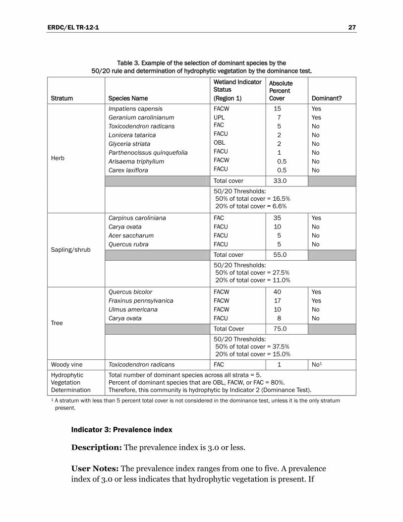
ERDC/EL TR-12-1 27
Table 3. Example of the selection of dominant species by the 50/20 rule and determination of hydrophytic vegetation by the dominance test.
Stratum Species Name
Wetland Indicator Status (Region 1)
Absolute Percent Cover Dominant?
Herb
Impatiens capensis Geranium carolinianum Toxicodendron radicans Lonicera tatarica Glyceria striata Parthenocissus quinquefolia Arisaema triphyllum Carex laxiflora
FACW UPL FAC FACU OBL FACU FACW FACU
15 7 5 2 2 1 0.5 0.5
Yes Yes No No No No No No
Total cover 33.0 50/20 Thresholds:
50% of total cover = 16.5% 20% of total cover = 6.6%
Sapling/shrub
Carpinus caroliniana Carya ovata Acer saccharum Quercus rubra
FAC FACU FACU FACU
35 10
5 5
Yes No No No
Total cover 55.0 50/20 Thresholds:
50% of total cover = 27.5% 20% of total cover = 11.0%
Tree
Quercus bicolor Fraxinus pennsylvanica Ulmus americana Carya ovata
FACW FACW FACW FACU
40 17 10
8
Yes Yes No No
Total Cover 75.0 50/20 Thresholds:
50% of total cover = 37.5% 20% of total cover = 15.0%
Woody vine Toxicodendron radicans FAC 1 No1 Hydrophytic Vegetation Determination
Total number of dominant species across all strata = 5. Percent of dominant species that are OBL, FACW, or FAC = 80%. Therefore, this community is hydrophytic by Indicator 2 (Dominance Test).
1 A stratum with less than 5 percent total cover is not considered in the dominance test, unless it is the only stratum present.
Indicator 3: Prevalence index
Description: The prevalence index is 3.0 or less.
User Notes: The prevalence index ranges from one to five. A prevalence index of 3.0 or less indicates that hydrophytic vegetation is present. If
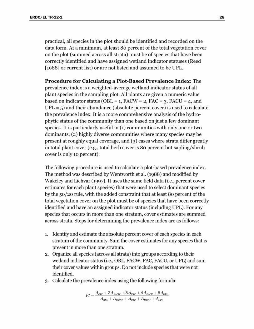
ERDC/EL TR-12-1 28
practical, all species in the plot should be identified and recorded on the data form. At a minimum, at least 80 percent of the total vegetation cover on the plot (summed across all strata) must be of species that have been correctly identified and have assigned wetland indicator statuses (Reed [1988] or current list) or are not listed and assumed to be UPL.
Procedure for Calculating a Plot-Based Prevalence Index: The prevalence index is a weighted-average wetland indicator status of all plant species in the sampling plot. All plants are given a numeric value based on indicator status (OBL = 1, FACW = 2, FAC = 3, FACU = 4, and UPL = 5) and their abundance (absolute percent cover) is used to calculate the prevalence index. It is a more comprehensive analysis of the hydro-phytic status of the community than one based on just a few dominant species. It is particularly useful in (1) communities with only one or two dominants, (2) highly diverse communities where many species may be present at roughly equal coverage, and (3) cases where strata differ greatly in total plant cover (e.g., total herb cover is 80 percent but sapling/shrub cover is only 10 percent).
The following procedure is used to calculate a plot-based prevalence index. The method was described by Wentworth et al. (1988) and modified by Wakeley and Lichvar (1997). It uses the same field data (i.e., percent cover estimates for each plant species) that were used to select dominant species by the 50/20 rule, with the added constraint that at least 80 percent of the total vegetation cover on the plot must be of species that have been correctly identified and have an assigned indicator status (including UPL). For any species that occurs in more than one stratum, cover estimates are summed across strata. Steps for determining the prevalence index are as follows:
1. Identify and estimate the absolute percent cover of each species in each stratum of the community. Sum the cover estimates for any species that is present in more than one stratum.
2. Organize all species (across all strata) into groups according to their wetland indicator status (i.e., OBL, FACW, FAC, FACU, or UPL) and sum their cover values within groups. Do not include species that were not identified.
3. Calculate the prevalence index using the following formula:
OBL FACW FAC FACU UPL
OBL FACW FAC FACU UPL
A A A A API
A A A A A
2 3 4 5
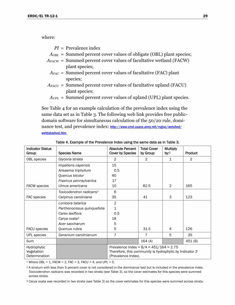
ERDC/EL TR-12-1 29
where:
PI = Prevalence index AOBL = Summed percent cover values of obligate (OBL) plant species; AFACW = Summed percent cover values of facultative wetland (FACW)
plant species; AFAC = Summed percent cover values of facultative (FAC) plant
species; AFACU = Summed percent cover values of facultative upland (FACU)
plant species; AUPL = Summed percent cover values of upland (UPL) plant species.
See Table 4 for an example calculation of the prevalence index using the same data set as in Table 3. The following web link provides free public-domain software for simultaneous calculation of the 50/20 rule, domi-nance test, and prevalence index:
Table 4. Example of the Prevalence Index using the same data as in Table 3.
http://www.crrel.usace.army.mil/rsgisc/wetshed/ wetdatashed.htm.
Indicator Status Group Species Name
Absolute Percent Cover by Species
Total Cover by Group
Multiply by:1 Product
OBL species Glyceria striata 2 2 1 2
FACW species
Impatiens capensis Arisaema triphyllum Quercus bicolor Fraxinus pennsylvanica Ulmus americana
15 0.5
40 17 10
82.5
2
165
FAC species Toxicodendron radicans2 Carpinus caroliniana
6 35
41
3
123
FACU species
Lonicera tatarica Parthenocissus quinquefolia Carex laxiflora Carya ovata3 Acer saccharum Quercus rubra
2 1 0.5
18 5 5
31.5
4
126 UPL species Geranium carolinianum 7 7 5 35 Sum 164 (A) 451 (B) Hydrophytic Vegetation Determination
Prevalence Index = B/A = 451/164 = 2.75 Therefore, this community is hydrophytic by Indicator 3 (Prevalence Index).
1 Where OBL = 1, FACW = 2, FAC = 3, FACU = 4, and UPL = 5. 2 A stratum with less than 5 percent cover is not considered in the dominance test but is included in the prevalence index.
Toxicodendron radicans was recorded in two strata (see Table 3), so the cover estimates for this species were summed across strata.
3 Carya ovata was recorded in two strata (see Table 3) so the cover estimates for this species were summed across strata.
ERDC/EL TR-12-1 30
Indicator 4: Morphological adaptations
Description: The plant community passes either the dominance test (Indicator 2) or the prevalence index (Indicator 3) after reconsideration of the indicator status of certain plant species that exhibit morphological adaptations for life in wetlands.
User Notes: Some hydrophytes in the Northcentral and Northeast Region develop easily recognized physical characteristics, or morpho-logical adaptations, when they occur in wetland areas. Some of these adaptations may help them to survive prolonged inundation or saturation in the root zone; others may simply be a consequence of living under such wet conditions. Common morphological adaptations in the region include, but are not limited to, adventitious roots, hypertrophied lenticels, multi-stemmed trunks, and shallow root systems developed on or near the soil surface (Figure 4). Users need to be cautious that shallow roots were not caused by erosion, near-surface bedrock, or rocky till, and that multi-trunk plants were not the result of sprouting after logging or browsing. Morphological adaptations may develop on FACU species when they occur in wetlands, indicating that those individuals are functioning as hydro-phytes in that setting.
To apply this indicator, these morphological features must be observed on more than 50 percent of the individuals of a FACU species living in an area where indicators of hydric soil and wetland hydrology are present. Follow this procedure:
1. Confirm that the morphological feature is present mainly in the potential wetland area and is not also common on the same species in the sur-rounding non-wetlands.
2. For each FACU species that exhibits morphological adaptations, estimate the percentage of individuals that have the features. Record this per-centage on the data form.
3. If more than 50 percent of the individuals of a FACU species have morpho-logical adaptations for life in wetlands, that species is considered to be a hydrophyte and its indicator status on that plot should be reassigned as FAC. All other species retain their published indicator statuses. Record any supporting information on the data sheet, including a description of the morphological adaptation(s) present and any other observations of the growth habit of the species in adjacent wetland and non-wetland locations (photo documentation is recommended).
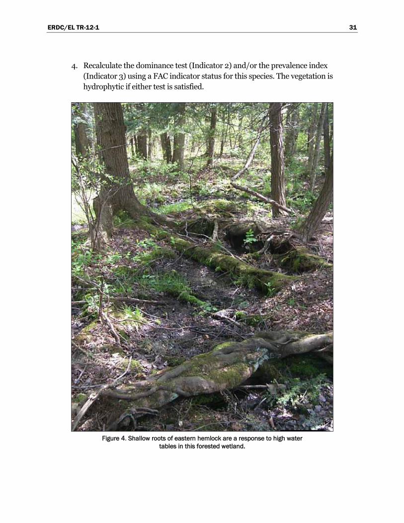
ERDC/EL TR-12-1 31
4. Recalculate the dominance test (Indicator 2) and/or the prevalence index (Indicator 3) using a FAC indicator status for this species. The vegetation is hydrophytic if either test is satisfied.
Figure 4. Shallow roots of eastern hemlock are a response to high water
tables in this forested wetland.
ERDC/EL TR-12-1 32
3 Hydric Soil Indicators Introduction
The National Technical Committee for Hydric Soils (NTCHS) defines a hydric soil as a soil that formed under conditions of saturation, flooding, or ponding long enough during the growing season to develop anaerobic conditions in the upper part (USDA Soil Conservation Service 1994). Most hydric soils exhibit characteristic morphologies that result from repeated periods of saturation or inundation for more than a few days. Saturation or inundation, when combined with microbial activity in the soil, causes the depletion of oxygen. This anaerobiosis promotes certain biogeochemical processes, such as the accumulation of organic matter and the reduction, translocation, or accumulation of iron and other reducible elements. These processes result in distinctive characteristics that persist in the soil during both wet and dry periods, making them particularly useful for identifying hydric soils in the field (USDA Natural Resources Conservation Service 2010).
This chapter presents indicators that are designed to help identify hydric soils in the Northcentral and Northeast Region. Indicators are not intended to replace or relieve the requirements contained in the definition of a hydric soil. Therefore, a soil that meets the definition of a hydric soil is hydric whether or not it exhibits indicators. Guidance for identifying hydric soils that lack indicators can be found later in this chapter (see the sections on documenting the site and its soils) and in Chapter 5 (Difficult Wetland Situations in the Northcentral and Northeast Region).
This list of indicators is dynamic; changes and additions to the list are anticipated with new research and field testing. The indicators presented in this supplement are a subset of the NTCHS Field Indicators of Hydric Soils in the United States (USDA Natural Resources Conservation Service [2010 or current version) that are commonly found in the region. Any change to the NTCHS Field Indicators of Hydric Soils in the United States represents a change to this subset of indicators for the Northcentral and Northeast Region. The current version of the indicators can be found on the NRCS hydric soils web site (http://soils.usda.gov/use/hydric). To use the indicators properly, a basic knowledge of soil/landscape relationships is necessary.
ERDC/EL TR-12-1 33
Most of the hydric soil indicators presented in this Supplement are applicable throughout the region; however, some are specific to certain subregions. As used in this supplement, subregions are equivalent to the Land Resource Regions (LRR) or Major Land Resource Areas (MLRA) recognized by the USDA Natural Resources Conservation Service (2006) (see Chapter 1, Figure 1). It is important to understand that boundaries between subregions are actually broad transition zones. Although an indi-cator may be noted as most relevant in a specific subregion, it may also be applicable in the transition to an adjacent subregion.
Concepts
Hydric soil indicators are formed predominantly by the accumulation or loss of iron, manganese, sulfur, or carbon compounds in a saturated and anaerobic environment. These processes and the features that develop are described in the following paragraphs.
Iron and manganese reduction, translocation, and accumulation
In an anaerobic environment, soil microbes reduce iron from the ferric (Fe3+) to the ferrous (Fe2+) form, and manganese from the manganic (Mn4+) to the manganous (Mn2+) form. Of the two, evidence of iron reduc-tion is more commonly observed in soils. Areas in the soil where iron is reduced often develop characteristic bluish-gray or greenish-gray colors known as gley. Ferric iron is insoluble but ferrous iron easily enters the soil solution and may be moved or translocated to other areas of the soil. Areas that have lost iron typically develop characteristic gray or reddish-gray colors and are known as redox depletions. If a soil reverts to an aerobic state, iron that is in solution will oxidize and become concentrated in patches and along root channels and other pores. These areas of oxi-dized iron are called redox concentrations. Since water movement in these saturated or inundated soils can be multi-directional, redox depletions and concentrations can occur anywhere in the soil and have irregular shapes and sizes. Soils that are saturated and contain ferrous iron at the time of sampling may change color upon exposure to the air, as ferrous iron is rapidly converted to ferric iron in the presence of oxygen. Such soils are said to have a reduced matrix (Vepraskas 1992).
While indicators related to iron or manganese depletion or concentration are the most common in hydric soils, they cannot form in soils whose parent materials are low in Fe or Mn. Soils formed in such materials may
ERDC/EL TR-12-1 34
have low-chroma colors that are not related to saturation and reduction. For such soils, features formed through accumulation of organic carbon may be present.
Sulfate reduction
Sulfur is one of the last elements to be reduced by microbes in an anae-robic environment. The microbes convert SO42− to H2S, or hydrogen sulfide gas. This results in a very pronounced “rotten egg” odor in some soils that are inundated or saturated for very long periods. In non-saturated or non-inundated soils, sulfate is not reduced and there is no rotten egg odor. The presence of hydrogen sulfide is a strong indicator of a hydric soil, but this indicator is found only in the wettest sites in soils that contain sulfur-bearing compounds.
Organic matter accumulation
Soil microbes use carbon compounds found in organic matter as an energy source. However, the rate at which organic carbon is utilized by soil mic-robes is considerably lower in a saturated and anaerobic environment than under aerobic conditions. Therefore, in saturated soils, partially decom-posed organic matter may accumulate. The result in wetlands is often the development of thick organic surfaces, such as peat or muck, or dark organic-rich mineral surface layers.
Non-saturated or non-inundated organic soils. In northern regions, cool temperatures and acid conditions slow the decomposition of organic matter. Under these conditions, even some well-drained soils, under predominantly aerobic conditions, can develop thick organic surface layers called folistic epipedons. These layers are not necessarily related to wetness. Folistic layers are organic accumulations that are saturated less than 30 days cumulatively in normal years (USDA Natural Resources Conservation Service 1999). Most folistic layers consist of poorly decom-posed organic material (i.e., fibric or hemic material; see the following section) although some consist of highly decomposed (i.e., sapric) mate-rial. Folistic surface layers may overlie rock, a mineral layer, or saturated organic layers, and are most commonly found on north- and east-facing slopes, in dense shade, and on nearly level, convex landforms in coniferous or mixed deciduous/coniferous forests in the colder, northern or high-elevation portions of the region. It may be necessary to involve a soil
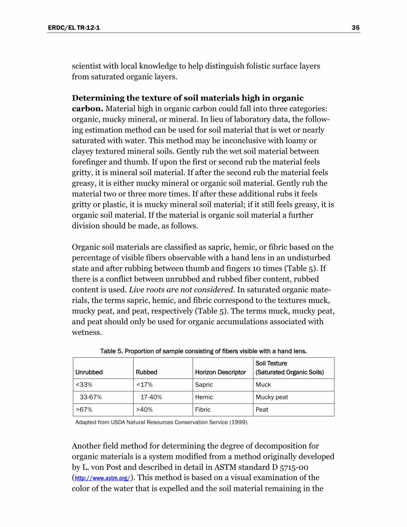
ERDC/EL TR-12-1 35
scientist with local knowledge to help distinguish folistic surface layers from saturated organic layers.
Determining the texture of soil materials high in organic carbon. Material high in organic carbon could fall into three categories: organic, mucky mineral, or mineral. In lieu of laboratory data, the follow-ing estimation method can be used for soil material that is wet or nearly saturated with water. This method may be inconclusive with loamy or clayey textured mineral soils. Gently rub the wet soil material between forefinger and thumb. If upon the first or second rub the material feels gritty, it is mineral soil material. If after the second rub the material feels greasy, it is either mucky mineral or organic soil material. Gently rub the material two or three more times. If after these additional rubs it feels gritty or plastic, it is mucky mineral soil material; if it still feels greasy, it is organic soil material. If the material is organic soil material a further division should be made, as follows.
Organic soil materials are classified as sapric, hemic, or fibric based on the percentage of visible fibers observable with a hand lens in an undisturbed state and after rubbing between thumb and fingers 10 times (Table 5). If there is a conflict between unrubbed and rubbed fiber content, rubbed content is used. Live roots are not considered. In saturated organic mate-rials, the terms sapric, hemic, and fibric correspond to the textures muck, mucky peat, and peat, respectively (Table 5). The terms muck, mucky peat, and peat should only be used for organic accumulations associated with wetness.
Table 5. Proportion of sample consisting of fibers visible with a hand lens.
Unrubbed Rubbed Horizon Descriptor Soil Texture (Saturated Organic Soils)
<33% <17% Sapric Muck
33-67% 17-40% Hemic Mucky peat
>67% >40% Fibric Peat
Adapted from USDA Natural Resources Conservation Service (1999).
Another field method for determining the degree of decomposition for organic materials is a system modified from a method originally developed by L. von Post and described in detail in ASTM standard D 5715-00 (http://www.astm.org/). This method is based on a visual examination of the color of the water that is expelled and the soil material remaining in the
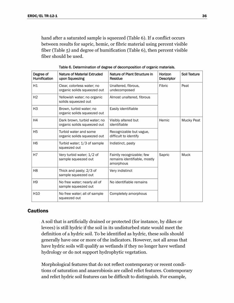
ERDC/EL TR-12-1 36
hand after a saturated sample is squeezed (Table 6). If a conflict occurs between results for sapric, hemic, or fibric material using percent visible fiber (Table 5) and degree of humification (Table 6), then percent visible fiber should be used.
Table 6. Determination of degree of decomposition of organic materials.
Degree of Humification
Nature of Material Extruded upon Squeezing
Nature of Plant Structure in Residue
Horizon Descriptor
Soil Texture
H1 Clear, colorless water; no organic solids squeezed out
Unaltered, fibrous, undecomposed
Fibric Peat
H2 Yellowish water; no organic solids squeezed out
Almost unaltered, fibrous
H3 Brown, turbid water; no organic solids squeezed out
Easily identifiable
H4 Dark brown, turbid water; no organic solids squeezed out
Visibly altered but identifiable
Hemic Mucky Peat
H5 Turbid water and some organic solids squeezed out
Recognizable but vague, difficult to identify
H6 Turbid water; 1/3 of sample squeezed out
Indistinct, pasty
H7 Very turbid water; 1/2 of sample squeezed out
Faintly recognizable; few remains identifiable, mostly amorphous
Sapric Muck
H8 Thick and pasty; 2/3 of sample squeezed out
Very indistinct
H9 No free water; nearly all of sample squeezed out
No identifiable remains
H10 No free water; all of sample squeezed out
Completely amorphous
Cautions
A soil that is artificially drained or protected (for instance, by dikes or levees) is still hydric if the soil in its undisturbed state would meet the definition of a hydric soil. To be identified as hydric, these soils should generally have one or more of the indicators. However, not all areas that have hydric soils will qualify as wetlands if they no longer have wetland hydrology or do not support hydrophytic vegetation.
Morphological features that do not reflect contemporary or recent condi-tions of saturation and anaerobiosis are called relict features. Contemporary and relict hydric soil features can be difficult to distinguish. For example,
ERDC/EL TR-12-1 37
nodules and concretions that are actively forming often have gradual or diffuse boundaries, whereas relict or degrading nodules and concretions have sharp boundaries (Vepraskas 1992). Guidance for some of the most common problem hydric soils can be found in Chapter 5. When soil morphology seems inconsistent with the landscape, vegetation, or observable hydrology, it may be necessary to obtain the assistance of an experienced soil or wetland scientist to determine whether the soil is hydric.
Procedures for sampling soils
Observe and document the site
Before making any decision about the presence or absence of hydric soils, the overall site and how it interacts with the soil should be considered. The questions below, while not required to identify a hydric soil, can help to explain why a hydric soil is or is not present. Always look at the landscape features of the immediate site and compare them to the surrounding areas. Try to contrast the features of wet and dry sites that are in close proximity. When observing slope features, look first at the area immediately around the sampling point. For example, a nearly level bench or depression at the sampling point may be more important to site wetness than the overall landform on which it occurs. By understanding how water moves across the site, the reasons for the presence or absence of hydric soil indicators should be clear.
If one or more of the hydric soil indicators given later in this chapter is present, then the soil is hydric. If no hydric soil indicator is present, the additional site information below may be useful in documenting whether the soil is indeed non-hydric or if it might represent a “problem” hydric soil that meets the hydric soil definition despite the absence of indicators.
• Hydrology–Is standing water observed on the site or is water observed in the soil pit? What is the depth of the water table in the area? Is there indirect evidence of ponding or flooding?
• Slope–Is the site level or nearly level so that surface water does not run off readily, or is it steeper where surface water would run off from the soil?
• Slope shape–Is the surface concave (e.g., depressions), where water would tend to collect and possibly pond on the soil surface? On hillsides, are there convergent slopes (Figure 5), where surface or
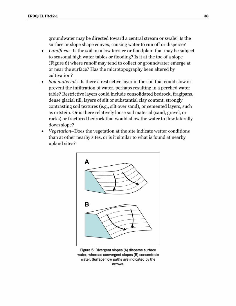
ERDC/EL TR-12-1 38
groundwater may be directed toward a central stream or swale? Is the surface or slope shape convex, causing water to run off or disperse?
• Landform–Is the soil on a low terrace or floodplain that may be subject to seasonal high water tables or flooding? Is it at the toe of a slope (Figure 6) where runoff may tend to collect or groundwater emerge at or near the surface? Has the microtopography been altered by cultivation?
• Soil materials–Is there a restrictive layer in the soil that could slow or prevent the infiltration of water, perhaps resulting in a perched water table? Restrictive layers could include consolidated bedrock, fragipans, dense glacial till, layers of silt or substantial clay content, strongly contrasting soil textures (e.g., silt over sand), or cemented layers, such as ortstein. Or is there relatively loose soil material (sand, gravel, or rocks) or fractured bedrock that would allow the water to flow laterally down slope?
• Vegetation–Does the vegetation at the site indicate wetter conditions than at other nearby sites, or is it similar to what is found at nearby upland sites?
Figure 5. Divergent slopes (A) disperse surface
water, whereas convergent slopes (B) concentrate water. Surface flow paths are indicated by the
arrows.
A
B
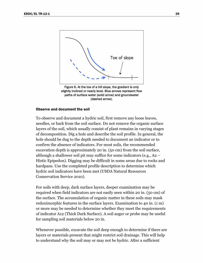
ERDC/EL TR-12-1 39
Figure 6. At the toe of a hill slope, the gradient is only
slightly inclined or nearly level. Blue arrows represent flow paths of surface water (solid arrow) and groundwater
(dashed arrow).
Observe and document the soil
To observe and document a hydric soil, first remove any loose leaves, needles, or bark from the soil surface. Do not remove the organic surface layers of the soil, which usually consist of plant remains in varying stages of decomposition. Dig a hole and describe the soil profile. In general, the hole should be dug to the depth needed to document an indicator or to confirm the absence of indicators. For most soils, the recommended excavation depth is approximately 20 in. (50 cm) from the soil surface, although a shallower soil pit may suffice for some indicators (e.g., A2 – Histic Epipedon). Digging may be difficult in some areas due to rocks and hardpans. Use the completed profile description to determine which hydric soil indicators have been met (USDA Natural Resources Conservation Service 2010).
For soils with deep, dark surface layers, deeper examination may be required when field indicators are not easily seen within 20 in. (50 cm) of the surface. The accumulation of organic matter in these soils may mask redoximorphic features in the surface layers. Examination to 40 in. (1 m) or more may be needed to determine whether they meet the requirements of indicator A12 (Thick Dark Surface). A soil auger or probe may be useful for sampling soil materials below 20 in.
Whenever possible, excavate the soil deep enough to determine if there are layers or materials present that might restrict soil drainage. This will help to understand why the soil may or may not be hydric. After a sufficient
ERDC/EL TR-12-1 40
number of exploratory excavations have been made to understand the soil-hydrologic relationships at the site, subsequent excavations can be limited to the depth needed to identify hydric soil indicators. Consider taking photographs of both the soil and the overall site, including a clearly marked measurement scale in soil pictures.
The starting point for depth measurements used in the indicators varies by Land Resource Region (LRR). In LRR R (Figure 1), depths are measured from the mineral surface (underneath any and all fibric, hemic, and/or sapric material), except for indicators A1 (Histosol), A2 (Histic Epipedon), A3 (Black Histic), and S3 (Mucky Peat or Peat) for which measurements begin at the actual soil surface. In all other LRRs in the Northcentral and Northeast Region, measurements begin at the muck or mineral surface (underneath any fibric and/or hemic material), except for indicators A1, A2, A3, and S3 where they begin at the actual soil surface (USDA Natural Resources Conservation Service 2010).
All colors noted in this supplement refer to moist Munsell® colors (Gretag/Macbeth 2000). Do not attempt to determine colors while wearing sunglasses or tinted lenses. Colors must be determined under natural light and not under artificial light.
Soil colors specified in the indicators do not have decimal points (except for indicator A12); however, intermediate colors do occur between Munsell chips. Soil color should not be rounded to qualify as meeting an indicator. For example, a soil matrix with a chroma between 2 and 3 should be recorded as having a chroma of 2+. This soil material does not have a chroma of 2 and would not meet any indicator that requires a chroma of 2 or less.
Always examine soil matrix colors in the field immediately after sampling. Ferrous iron, if present, can oxidize rapidly and create colors of higher chroma or redder hue. In soils that are saturated at the time of sampling, redox concentrations may be absent or difficult to see, particularly in dark-colored soils. It may be necessary to let the soil dry to a moist state (5 to 30 minutes or more) for the iron or manganese to oxidize and redox features to become visible.
Particular attention should be paid to changes in microtopography over short distances. Small changes in elevation may result in repetitive
ERDC/EL TR-12-1 41
sequences of hydric/non-hydric soils, making the delineation of individual areas of hydric and non-hydric soils difficult. Often the dominant con-dition (hydric or non-hydric) is the only reliable interpretation (also see the section on Wetland/Non-Wetland Mosaics in Chapter 5). The shape of the local landform can greatly affect the movement of water through the landscape. Significant changes in parent material or lithologic disconti-nuities in the soil can also affect the hydrologic properties of the soil.
Use of existing soil data
Soil surveys
Soil surveys are available for most areas of the Northcentral and Northeast Region and can provide useful information regarding soil properties and soil moisture conditions for an area. A list of available soil surveys is located at http://soils.usda.gov/survey/online_surveys/, and soil survey maps and data are available online from the Web Soil Survey at http://websoilsurvey.nrcs.usda.gov/. Soil survey maps divide the landscape into areas called map units. Map units usually contain more than one soil type or component. They often contain several minor components or inclusions of soils with properties that may be similar to or quite different from the major component. Some of these inclusions may be hydric while the major component is not, and vice versa. Those soils that are hydric are noted in the Hydric Soils List published separately from the soil survey report. Soil survey information can be valuable for planning purposes, but it is not site-specific and does not preclude the need for an on-site investigation.
Hydric soils lists
Hydric Soils Lists are developed for each detailed soil survey. Using criteria approved by the NTCHS, these lists rate each soil component as either hydric or non-hydric based on soil property data. If the soil is rated as hydric, information is provided regarding which hydric criteria are met and on what landform the soil typically occurs. Hydric Soils Lists are use-ful as general background information for an on-site delineation. The hydric soils list should be used as a tool, indicating that hydric soil will likely be found within a given area. However, not all areas within a polygon identified as having hydric soils may be hydric.
Hydric Soils Lists developed for individual detailed soil surveys are known as Local Hydric Soils Lists. They are available from state or county NRCS

ERDC/EL TR-12-1 42
offices and over the internet from the Soil Data Mart (http://soildatamart.nrcs.usda.gov/). Local Hydric Soils Lists have been compiled into a National Hydric Soils List available at http://soils.usda.gov/use/hydric/. However, use of Local Hydric Soils Lists is preferred since they are more current and reflect local variations in soil properties.
Hydric soil indicators
Many of the hydric soil indicators were developed specifically for wetland-delineation purposes. During the development of these indicators, soils in the interior of wetlands were not always examined; therefore, there are wetlands that lack any of the approved hydric soil indicators in the wettest interior portions. Wetland delineators and other users of the hydric soil indicators should concentrate their sampling efforts near the wetland edge and, if these soils are hydric, assume that soils in the wetter, interior portions of the wetland are also hydric, even if they lack an indicator.
Hydric soil indicators are presented in three groups. Indicators for “All Soils” are used in any soil regardless of texture. Indicators for “Sandy Soils” are used in soil layers with USDA textures of loamy fine sand or coarser. Indicators for “Loamy and Clayey Soils” are used with soil layers of loamy very fine sand and finer. Both sandy and loamy/clayey layers may be present in the same soil profile. Therefore, a soil that contains a loamy surface layer over sand is hydric if it meets all of the requirements of matrix color, amount and contrast of redox concentrations, depth, and thickness for a specific A (All Soils), F (Loamy and Clayey Soils), or S (Sandy Soils) indicator. Additional indicators for problematic hydric soils are presented on pages 71-79. These indicators are used in conjunction with the procedure given in Chapter 5.
It is permissible to combine certain hydric soil indicators if all require-ments of the individual indicators are met except thickness (see Hydric Soil Technical Note 4, http://soils.usda.gov/use/hydric/ntchs/tech_notes/index.html). The most restrictive requirements for thickness of layers in any indicators used must be met. Not all indicators are possible candidates for combination. For example, indicator F2 (Loamy Gleyed Matrix) has no thickness requirement, so a site would either meet the requirements of this indicator or it would not. Table 7 lists the indicators that are the most likely candi-dates for combining in the region.
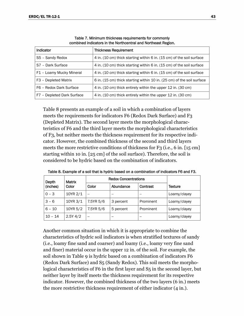
ERDC/EL TR-12-1 43
Table 7. Minimum thickness requirements for commonly combined indicators in the Northcentral and Northeast Region.
Indicator Thickness Requirement
S5 – Sandy Redox 4 in. (10 cm) thick starting within 6 in. (15 cm) of the soil surface
S7 – Dark Surface 4 in. (10 cm) thick starting within 6 in. (15 cm) of the soil surface
F1 – Loamy Mucky Mineral 4 in. (10 cm) thick starting within 6 in. (15 cm) of the soil surface
F3 – Depleted Matrix 6 in. (15 cm) thick starting within 10 in. (25 cm) of the soil surface
F6 – Redox Dark Surface 4 in. (10 cm) thick entirely within the upper 12 in. (30 cm)
F7 – Depleted Dark Surface 4 in. (10 cm) thick entirely within the upper 12 in. (30 cm)
Table 8 presents an example of a soil in which a combination of layers meets the requirements for indicators F6 (Redox Dark Surface) and F3 (Depleted Matrix). The second layer meets the morphological charac-teristics of F6 and the third layer meets the morphological characteristics of F3, but neither meets the thickness requirement for its respective indi-cator. However, the combined thickness of the second and third layers meets the more restrictive conditions of thickness for F3 (i.e., 6 in. [15 cm] starting within 10 in. [25 cm] of the soil surface). Therefore, the soil is considered to be hydric based on the combination of indicators.
Table 8. Example of a soil that is hydric based on a combination of indicators F6 and F3.
Depth (inches)
Matrix Color
Redox Concentrations
Texture Color Abundance Contrast
0 – 3 10YR 2/1 -- -- -- Loamy/clayey
3 – 6 10YR 3/1 7.5YR 5/6 3 percent Prominent Loamy/clayey
6 – 10 10YR 5/2 7.5YR 5/6 5 percent Prominent Loamy/clayey
10 – 14 2.5Y 4/2 -- -- -- Loamy/clayey
Another common situation in which it is appropriate to combine the characteristics of hydric soil indicators is when stratified textures of sandy (i.e., loamy fine sand and coarser) and loamy (i.e., loamy very fine sand and finer) material occur in the upper 12 in. of the soil. For example, the soil shown in Table 9 is hydric based on a combination of indicators F6 (Redox Dark Surface) and S5 (Sandy Redox). This soil meets the morpho-logical characteristics of F6 in the first layer and S5 in the second layer, but neither layer by itself meets the thickness requirement for its respective indicator. However, the combined thickness of the two layers (6 in.) meets the more restrictive thickness requirement of either indicator (4 in.).
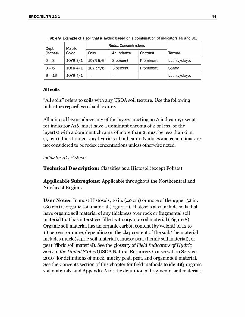
ERDC/EL TR-12-1 44
Table 9. Example of a soil that is hydric based on a combination of indicators F6 and S5.
Depth (inches)
Matrix Color
Redox Concentrations
Texture Color Abundance Contrast
0 – 3 10YR 3/1 10YR 5/6 3 percent Prominent Loamy/clayey
3 – 6 10YR 4/1 10YR 5/6 3 percent Prominent Sandy
6 – 16 10YR 4/1 -- -- -- Loamy/clayey
All soils
“All soils” refers to soils with any USDA soil texture. Use the following indicators regardless of soil texture.
All mineral layers above any of the layers meeting an A indicator, except for indicator A16, must have a dominant chroma of 2 or less, or the layer(s) with a dominant chroma of more than 2 must be less than 6 in. (15 cm) thick to meet any hydric soil indicator. Nodules and concretions are not considered to be redox concentrations unless otherwise noted.
Indicator A1: Histosol
Technical Description: Classifies as a Histosol (except Folists)
Applicable Subregions: Applicable throughout the Northcentral and Northeast Region.
User Notes: In most Histosols, 16 in. (40 cm) or more of the upper 32 in. (80 cm) is organic soil material (Figure 7). Histosols also include soils that have organic soil material of any thickness over rock or fragmental soil material that has interstices filled with organic soil material (Figure 8). Organic soil material has an organic carbon content (by weight) of 12 to 18 percent or more, depending on the clay content of the soil. The material includes muck (sapric soil material), mucky peat (hemic soil material), or peat (fibric soil material). See the glossary of Field Indicators of Hydric Soils in the United States (USDA Natural Resources Conservation Service 2010) for definitions of muck, mucky peat, peat, and organic soil material. See the Concepts section of this chapter for field methods to identify organic soil materials, and Appendix A for the definition of fragmental soil material.
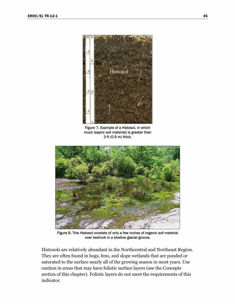
ERDC/EL TR-12-1 45
Figure 7. Example of a Histosol, in which
muck (sapric soil material) is greater than 3 ft (0.9 m) thick.
Figure 8. This Histosol consists of only a few inches of organic soil material
over bedrock in a shallow glacial groove.
Histosols are relatively abundant in the Northcentral and Northeast Region. They are often found in bogs, fens, and slope wetlands that are ponded or saturated to the surface nearly all of the growing season in most years. Use caution in areas that may have folistic surface layers (see the Concepts section of this chapter). Folistic layers do not meet the requirements of this indicator.
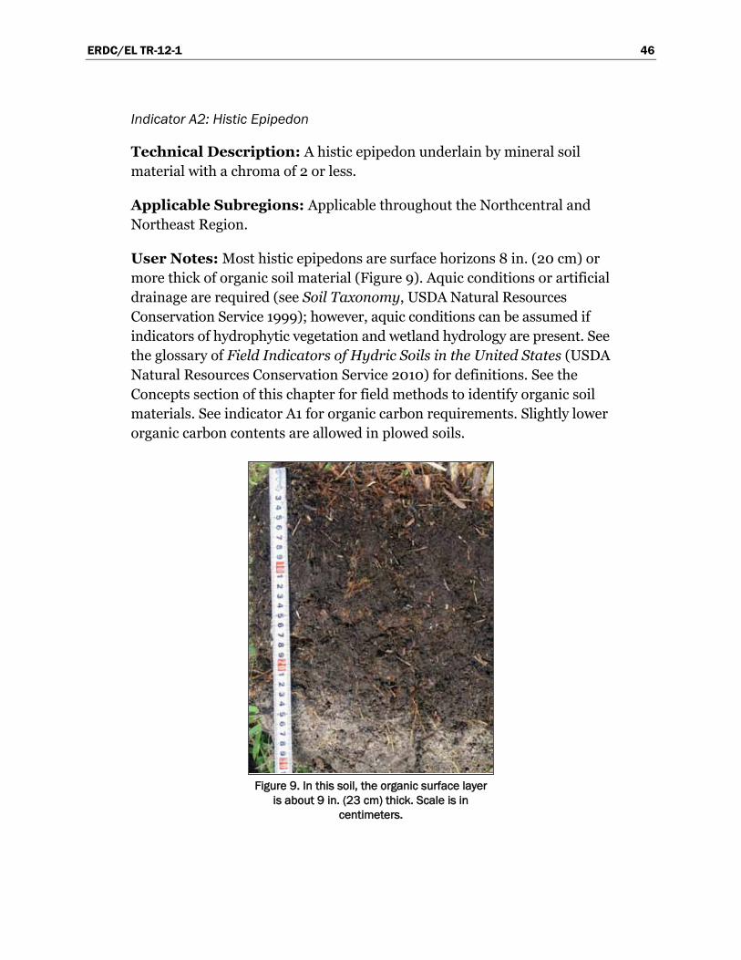
ERDC/EL TR-12-1 46
Indicator A2: Histic Epipedon
Technical Description: A histic epipedon underlain by mineral soil material with a chroma of 2 or less.
Applicable Subregions: Applicable throughout the Northcentral and Northeast Region.
User Notes: Most histic epipedons are surface horizons 8 in. (20 cm) or more thick of organic soil material (Figure 9). Aquic conditions or artificial drainage are required (see Soil Taxonomy, USDA Natural Resources Conservation Service 1999); however, aquic conditions can be assumed if indicators of hydrophytic vegetation and wetland hydrology are present. See the glossary of Field Indicators of Hydric Soils in the United States (USDA Natural Resources Conservation Service 2010) for definitions. See the Concepts section of this chapter for field methods to identify organic soil materials. See indicator A1 for organic carbon requirements. Slightly lower organic carbon contents are allowed in plowed soils.
Figure 9. In this soil, the organic surface layer
is about 9 in. (23 cm) thick. Scale is in centimeters.
ERDC/EL TR-12-1 47
This indicator is common in the region. It is often found in bogs, fens, and slope wetlands that are ponded or saturated to the surface nearly all of the growing season in most years.
Indicator A3: Black Histic
Technical Description: A layer of peat, mucky peat, or muck 8 in. (20 cm) or more thick that starts within 6 in. (15 cm) of the soil surface; has a hue of 10YR or yellower, value of 3 or less, and chroma of 1 or less; and is underlain by mineral soil material with a chroma of 2 or less.
Applicable Subregions: Applicable throughout the Northcentral and Northeast Region.
User Notes: This indicator does not require proof of aquic conditions or artificial drainage. See the glossary of Field Indicators of Hydric Soils in the United States (USDA Natural Resources Conservation Service 2010) for definitions of peat, mucky peat, and muck. See the Concepts section of this chapter for field methods to identify organic soil materials. See indicator A1 for organic carbon requirements.
This indicator is common in the region. It is often found in bogs, fens, and slope wetlands that are ponded or saturated to the surface nearly all of the growing season in most years.
Indicator A4: Hydrogen Sulfide
Technical Description: A hydrogen sulfide (rotten egg) odor within 12 in. (30 cm) of the soil surface.
Applicable Subregions: Applicable throughout the Northcentral and Northeast Region.
User Notes: Any time the soil smells of hydrogen sulfide (rotten egg odor), sulfur is currently being reduced and the soil is definitely in an anaerobic state. In some soils, the odor is pronounced; in others it is very fleeting as the gas dissipates rapidly. If in doubt, quickly open several small holes in the area of concern to determine if a hydrogen sulfide odor is really present. This indicator generally is not found at the boundaries between wetlands and non-wetlands. It is most commonly found in areas that are permanently saturated or inundated.
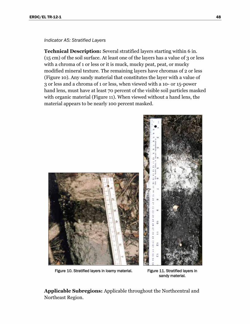
ERDC/EL TR-12-1 48
Indicator A5: Stratified Layers
Technical Description: Several stratified layers starting within 6 in. (15 cm) of the soil surface. At least one of the layers has a value of 3 or less with a chroma of 1 or less or it is muck, mucky peat, peat, or mucky modified mineral texture. The remaining layers have chromas of 2 or less (Figure 10). Any sandy material that constitutes the layer with a value of 3 or less and a chroma of 1 or less, when viewed with a 10- or 15-power hand lens, must have at least 70 percent of the visible soil particles masked with organic material (Figure 11). When viewed without a hand lens, the material appears to be nearly 100 percent masked.
Figure 10. Stratified layers in loamy material. Figure 11. Stratified layers in
sandy material.
Applicable Subregions: Applicable throughout the Northcentral and Northeast Region.
ERDC/EL TR-12-1 49
User Notes: Use of this indicator may require assistance from a soil scientist with local experience. An undisturbed sample must be observed. Individual strata are dominantly less than 1 in. (2.5 cm) thick. A hand lens can aid in the identification of this indicator. Many alluvial soils have stratified layers at depths greater than 6 in. (15 cm); these do not fit this indicator. Many alluvial soils have stratified layers at the required depths but lack a chroma of 2 or less; these do not fit this indicator. Stratified layers occur in any type of soil material, generally in floodplains and other areas where wet soils are subject to rapid and repeated burial with thin deposits of sediment.
Indicator A11: Depleted Below Dark Surface
Technical Description: A layer with a depleted or gleyed matrix that has 60 percent or more chroma of 2 or less, starting within 12 in. (30 cm) of the soil surface, and having a minimum thickness of either:
• 6 in. (15 cm), or • 2 in. (5 cm) if the 2 in. (5 cm) consists of fragmental soil material.
Loamy/clayey layer(s) above the depleted or gleyed matrix must have a value of 3 or less and chroma of 2 or less. Any sandy material above the depleted or gleyed matrix must have a value of 3 or less and chroma of 1 or less and, when viewed with a 10- or 15-power hand lens, must have at least 70 percent of the visible soil particles masked with organic material. When viewed without a hand lens, the material appears to be nearly 100 percent masked.
Applicable Subregions: Applicable throughout the Northcentral and Northeast Region.
User Notes: This indicator often occurs in hydric soils that have dark-colored surface layers, such as umbric epipedons and dark-colored ochric epipedons (Figure 12). For soils that have dark surface layers greater than 12 in. (30 cm) thick, use indicator A12. Two percent or more distinct or prominent redox concentrations, including iron/manganese soft masses, pore linings, or both, are required in soils that have matrix values/ chromas of 4/1, 4/2, and 5/2 (Figure A1). If the soil is saturated at the time of sampling, it may be necessary to let it dry to a moist condition for redox features to become visible. See the Glossary (Appendix A) for definitions of depleted matrix, gleyed matrix, distinct and prominent features, and fragmental soil material.
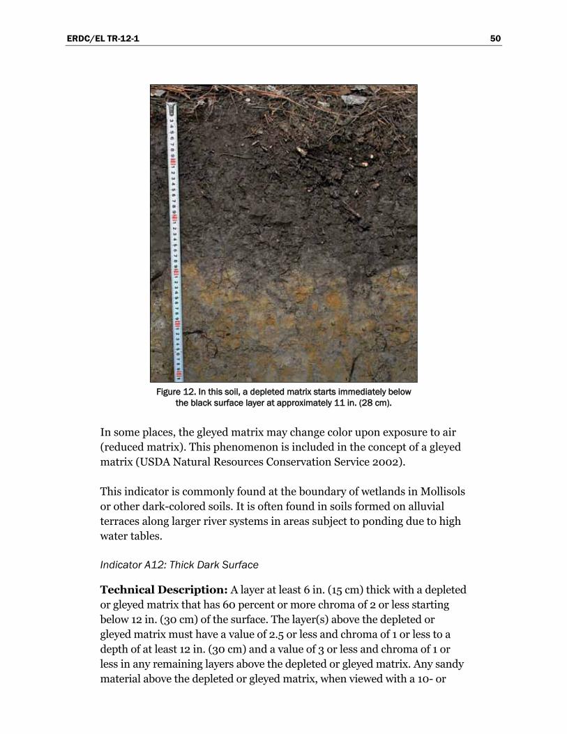
ERDC/EL TR-12-1 50
Figure 12. In this soil, a depleted matrix starts immediately below
the black surface layer at approximately 11 in. (28 cm).
In some places, the gleyed matrix may change color upon exposure to air (reduced matrix). This phenomenon is included in the concept of a gleyed matrix (USDA Natural Resources Conservation Service 2002).
This indicator is commonly found at the boundary of wetlands in Mollisols or other dark-colored soils. It is often found in soils formed on alluvial terraces along larger river systems in areas subject to ponding due to high water tables.
Indicator A12: Thick Dark Surface
Technical Description: A layer at least 6 in. (15 cm) thick with a depleted or gleyed matrix that has 60 percent or more chroma of 2 or less starting below 12 in. (30 cm) of the surface. The layer(s) above the depleted or gleyed matrix must have a value of 2.5 or less and chroma of 1 or less to a depth of at least 12 in. (30 cm) and a value of 3 or less and chroma of 1 or less in any remaining layers above the depleted or gleyed matrix. Any sandy material above the depleted or gleyed matrix, when viewed with a 10- or
ERDC/EL TR-12-1 51
15-power hand lens, must have at least 70 percent of the visible soil particles masked with organic material. When viewed without a hand lens, the material appears to be nearly 100 percent masked.
Applicable Subregions: Applicable throughout the Northcentral and Northeast Region.
User Notes: The soil has a depleted matrix or gleyed matrix below a black or very dark gray surface layer 12 in. (30 cm) or more thick (Figure 13). This indicator is most often associated with overthickened soils in concave landscape positions. Two percent or more distinct or prominent redox concentrations (Table A1), including iron/manganese soft masses, pore linings, or both, are required in soils that have matrix values/chromas of 4/1, 4/2, and 5/2 (Figure A1). If the soil is saturated at the time of sampling, it may be necessary to let it dry to a moist condition for redox features to become visible. See the Glossary (Appendix A) for the definitions of depleted and gleyed matrix.
In some places, the gleyed matrix may change color upon exposure to air (reduced matrix). This phenomenon is included in the concept of a gleyed matrix (USDA Natural Resources Conservation Service 2002).
This indicator is almost never found at the wetland/non-wetland boundary and is much less common than indicators A11 (Depleted Below Dark Surface), F3 (Depleted Matrix), and F6 (Redox Dark Surface).
Sandy soils
“Sandy soils” refers to soil materials with a USDA soil texture of loamy fine sand and coarser. Use the following indicators in soil layers consisting of sandy soil materials.
All mineral layers above any of the layers meeting an S indicator, except for indicator S6, must have a dominant chroma of 2 or less, or the layer(s) with a dominant chroma of more than 2 must be less than 6 in. (15 cm) thick to meet any hydric soil indicator. Nodules and concretions are not considered to be redox concentrations unless otherwise noted.
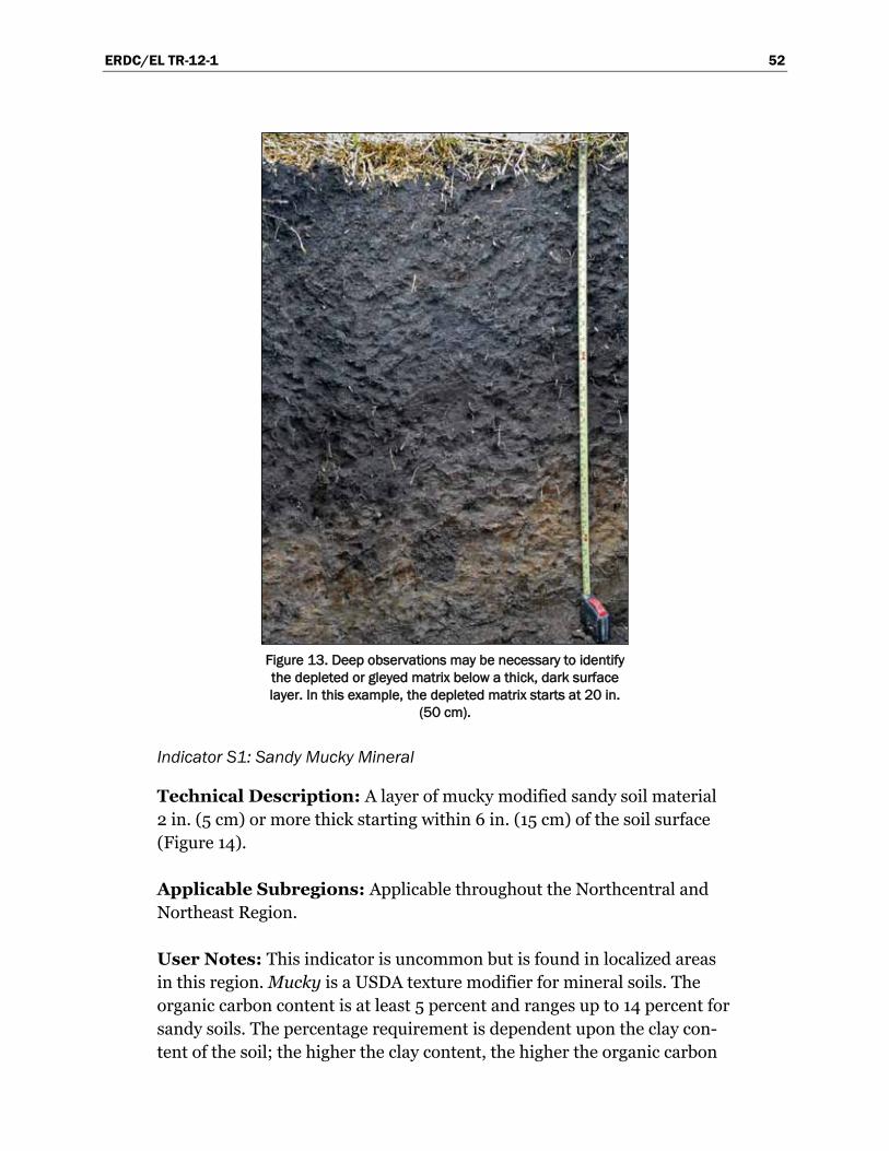
ERDC/EL TR-12-1 52
Figure 13. Deep observations may be necessary to identify the depleted or gleyed matrix below a thick, dark surface layer. In this example, the depleted matrix starts at 20 in.
(50 cm).
Indicator S1: Sandy Mucky Mineral
Technical Description: A layer of mucky modified sandy soil material 2 in. (5 cm) or more thick starting within 6 in. (15 cm) of the soil surface (Figure 14).
Applicable Subregions: Applicable throughout the Northcentral and Northeast Region.
User Notes: This indicator is uncommon but is found in localized areas in this region. Mucky is a USDA texture modifier for mineral soils. The organic carbon content is at least 5 percent and ranges up to 14 percent for sandy soils. The percentage requirement is dependent upon the clay con-tent of the soil; the higher the clay content, the higher the organic carbon
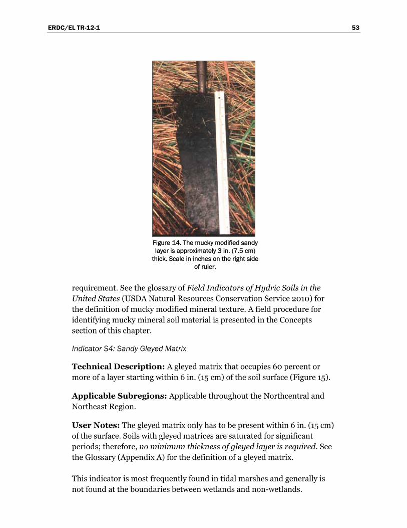
ERDC/EL TR-12-1 53
Figure 14. The mucky modified sandy layer is approximately 3 in. (7.5 cm)
thick. Scale in inches on the right side of ruler.
requirement. See the glossary of Field Indicators of Hydric Soils in the United States (USDA Natural Resources Conservation Service 2010) for the definition of mucky modified mineral texture. A field procedure for identifying mucky mineral soil material is presented in the Concepts section of this chapter.
Indicator S4: Sandy Gleyed Matrix
Technical Description: A gleyed matrix that occupies 60 percent or more of a layer starting within 6 in. (15 cm) of the soil surface (Figure 15).
Applicable Subregions: Applicable throughout the Northcentral and Northeast Region.
User Notes: The gleyed matrix only has to be present within 6 in. (15 cm) of the surface. Soils with gleyed matrices are saturated for significant periods; therefore, no minimum thickness of gleyed layer is required. See the Glossary (Appendix A) for the definition of a gleyed matrix.
This indicator is most frequently found in tidal marshes and generally is not found at the boundaries between wetlands and non-wetlands.
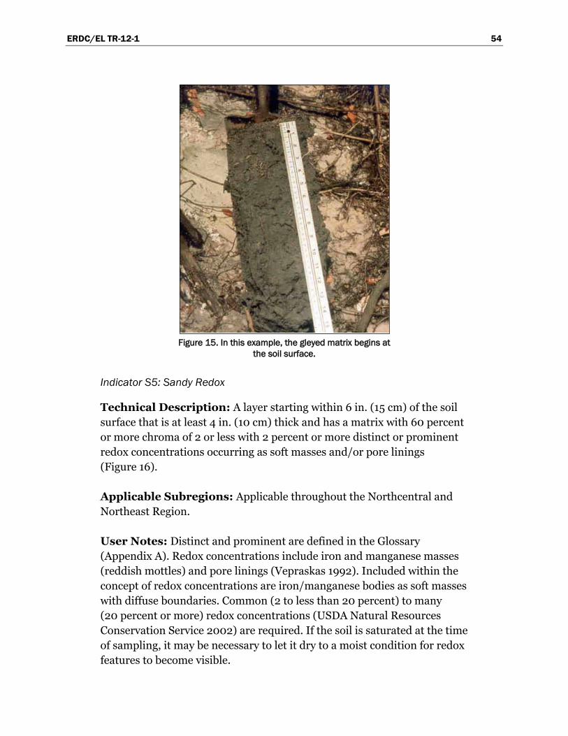
ERDC/EL TR-12-1 54
Figure 15. In this example, the gleyed matrix begins at
the soil surface.
Indicator S5: Sandy Redox
Technical Description: A layer starting within 6 in. (15 cm) of the soil surface that is at least 4 in. (10 cm) thick and has a matrix with 60 percent or more chroma of 2 or less with 2 percent or more distinct or prominent redox concentrations occurring as soft masses and/or pore linings (Figure 16).
Applicable Subregions: Applicable throughout the Northcentral and Northeast Region.
User Notes: Distinct and prominent are defined in the Glossary (Appendix A). Redox concentrations include iron and manganese masses (reddish mottles) and pore linings (Vepraskas 1992). Included within the concept of redox concentrations are iron/manganese bodies as soft masses with diffuse boundaries. Common (2 to less than 20 percent) to many (20 percent or more) redox concentrations (USDA Natural Resources Conservation Service 2002) are required. If the soil is saturated at the time of sampling, it may be necessary to let it dry to a moist condition for redox features to become visible.
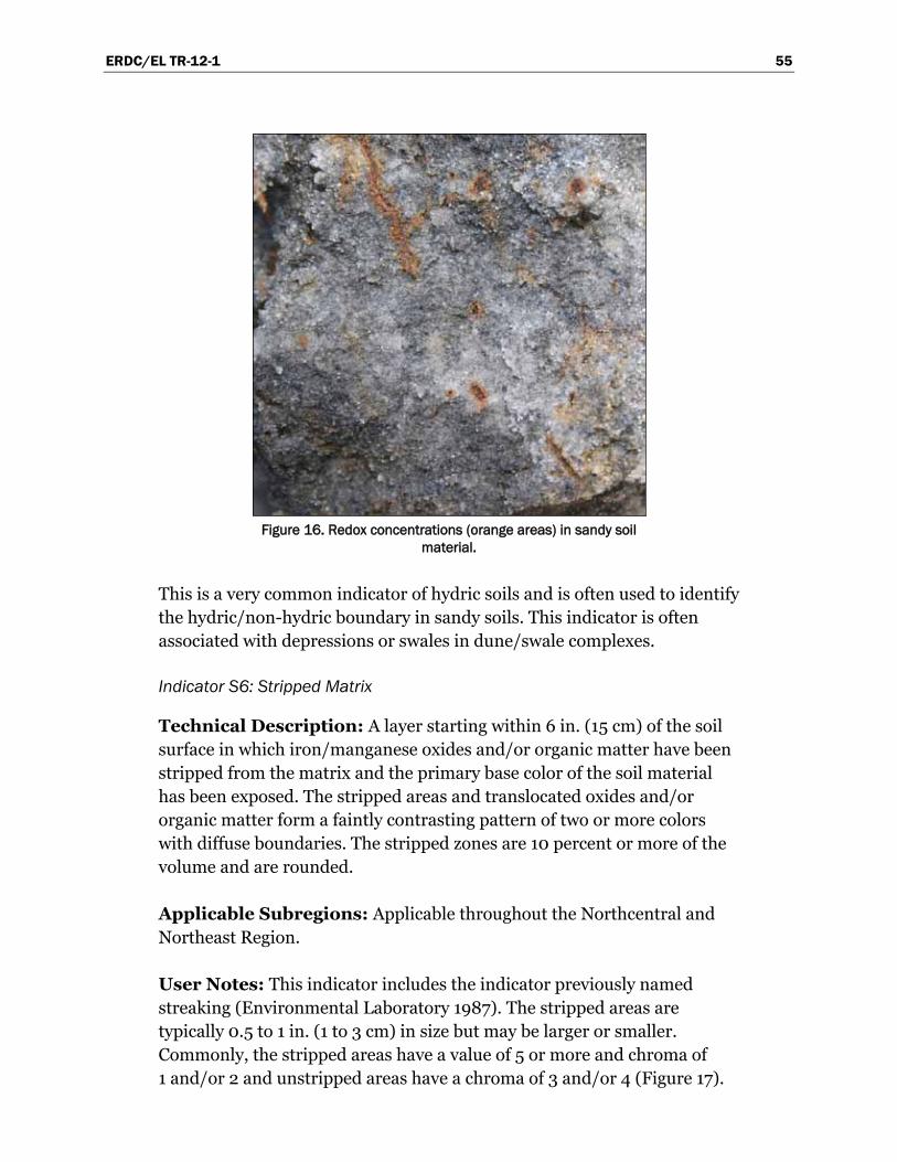
ERDC/EL TR-12-1 55
Figure 16. Redox concentrations (orange areas) in sandy soil
material.
This is a very common indicator of hydric soils and is often used to identify the hydric/non-hydric boundary in sandy soils. This indicator is often associated with depressions or swales in dune/swale complexes.
Indicator S6: Stripped Matrix
Technical Description: A layer starting within 6 in. (15 cm) of the soil surface in which iron/manganese oxides and/or organic matter have been stripped from the matrix and the primary base color of the soil material has been exposed. The stripped areas and translocated oxides and/or organic matter form a faintly contrasting pattern of two or more colors with diffuse boundaries. The stripped zones are 10 percent or more of the volume and are rounded.
Applicable Subregions: Applicable throughout the Northcentral and Northeast Region.
User Notes: This indicator includes the indicator previously named streaking (Environmental Laboratory 1987). The stripped areas are typically 0.5 to 1 in. (1 to 3 cm) in size but may be larger or smaller. Commonly, the stripped areas have a value of 5 or more and chroma of 1 and/or 2 and unstripped areas have a chroma of 3 and/or 4 (Figure 17).
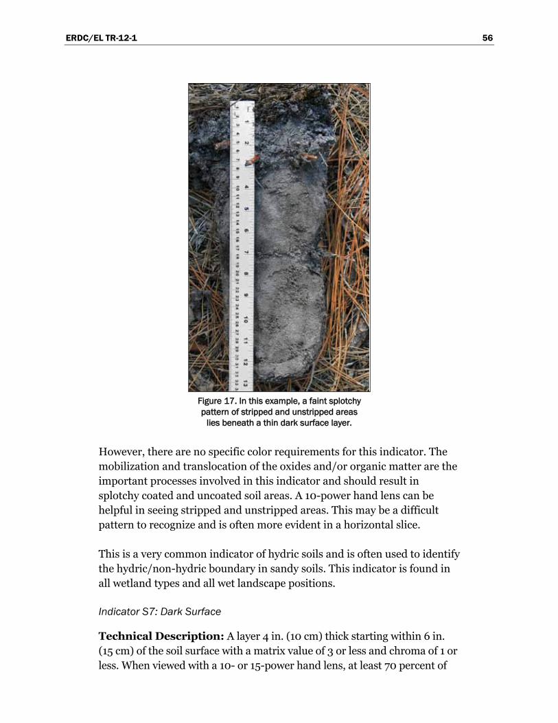
ERDC/EL TR-12-1 56
Figure 17. In this example, a faint splotchy pattern of stripped and unstripped areas
lies beneath a thin dark surface layer.
However, there are no specific color requirements for this indicator. The mobilization and translocation of the oxides and/or organic matter are the important processes involved in this indicator and should result in splotchy coated and uncoated soil areas. A 10-power hand lens can be helpful in seeing stripped and unstripped areas. This may be a difficult pattern to recognize and is often more evident in a horizontal slice.
This is a very common indicator of hydric soils and is often used to identify the hydric/non-hydric boundary in sandy soils. This indicator is found in all wetland types and all wet landscape positions.
Indicator S7: Dark Surface
Technical Description: A layer 4 in. (10 cm) thick starting within 6 in. (15 cm) of the soil surface with a matrix value of 3 or less and chroma of 1 or less. When viewed with a 10- or 15-power hand lens, at least 70 percent of
ERDC/EL TR-12-1 57
the visible soil particles must be masked with organic material. When viewed without a hand lens, the material appears to be nearly 100 percent masked. The matrix color of the layer immediately below the dark layer must have the same colors as those described above or any color that has a chroma of 2 or less.
Applicable Subregions: Applicable to the Northeastern Forests Sub-region (LRR R) (Figure 1) and the Long Island/Cape Cod Subregion (MLRA 149B of LRR S) (Figure 18). For testing in LRRs K, L, and M.
User Notes: If the dark layer is greater than 4 in. (10 cm) thick, then the indicator is met, because any dark soil material in excess of 4 in. (10 cm) meets the requirement that “the layer immediately below the dark layer must have the same colors as those described above… .” If the dark layer is exactly 4 in. (10 cm) thick, then the material immediately below must have a matrix chroma of 2 or less.
This indicator is applicable to interdunal swales along the Atlantic Ocean. The organic carbon content of this indicator is slightly less than that required for “mucky.” An undisturbed sample must be observed (Figure 19). Many moderately wet soils have a ratio of about 50 percent of soil particles covered or coated with organic matter to about 50 percent uncoated or uncovered soil particles, giving the soil a salt-and-pepper appearance. Where the percent coverage by organic matter is less than 70 percent, the Dark Surface indicator is not present.
Indicator S8: Polyvalue Below Surface
Technical Description: A layer with a value of 3 or less and chroma of 1 or less starting within 6 in. (15 cm) of the soil surface. When viewed with a 10- or 15-power hand lens, at least 70 percent of the visible soil particles in this layer must be masked with organic material. When viewed without a hand lens, the material appears to be nearly 100 percent masked. Immediately below this layer, 5 percent or more of the soil volume has a value of 3 or less and chroma of 1 or less and the remainder of the soil volume has a value of 4 or more and chroma of 1 or less to a depth of 12 in. (30 cm) or to the spodic horizon, whichever is less.
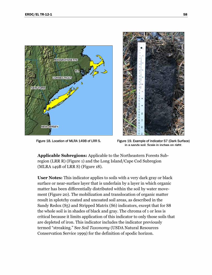
ERDC/EL TR-12-1 58
Figure 18. Location of MLRA 149B of LRR S. Figure 19. Example of indicator S7 (Dark Surface) in a sandy soil. Scale in inches on right.
Applicable Subregions: Applicable to the Northeastern Forests Sub-region (LRR R) (Figure 1) and the Long Island/Cape Cod Subregion (MLRA 149B of LRR S) (Figure 18).
User Notes: This indicator applies to soils with a very dark gray or black surface or near-surface layer that is underlain by a layer in which organic matter has been differentially distributed within the soil by water move-ment (Figure 20). The mobilization and translocation of organic matter result in splotchy coated and uncoated soil areas, as described in the Sandy Redox (S5) and Stripped Matrix (S6) indicators, except that for S8 the whole soil is in shades of black and gray. The chroma of 1 or less is critical because it limits application of this indicator to only those soils that are depleted of iron. This indicator includes the indicator previously termed “streaking.” See Soil Taxonomy (USDA Natural Resources Conservation Service 1999) for the definition of spodic horizon.
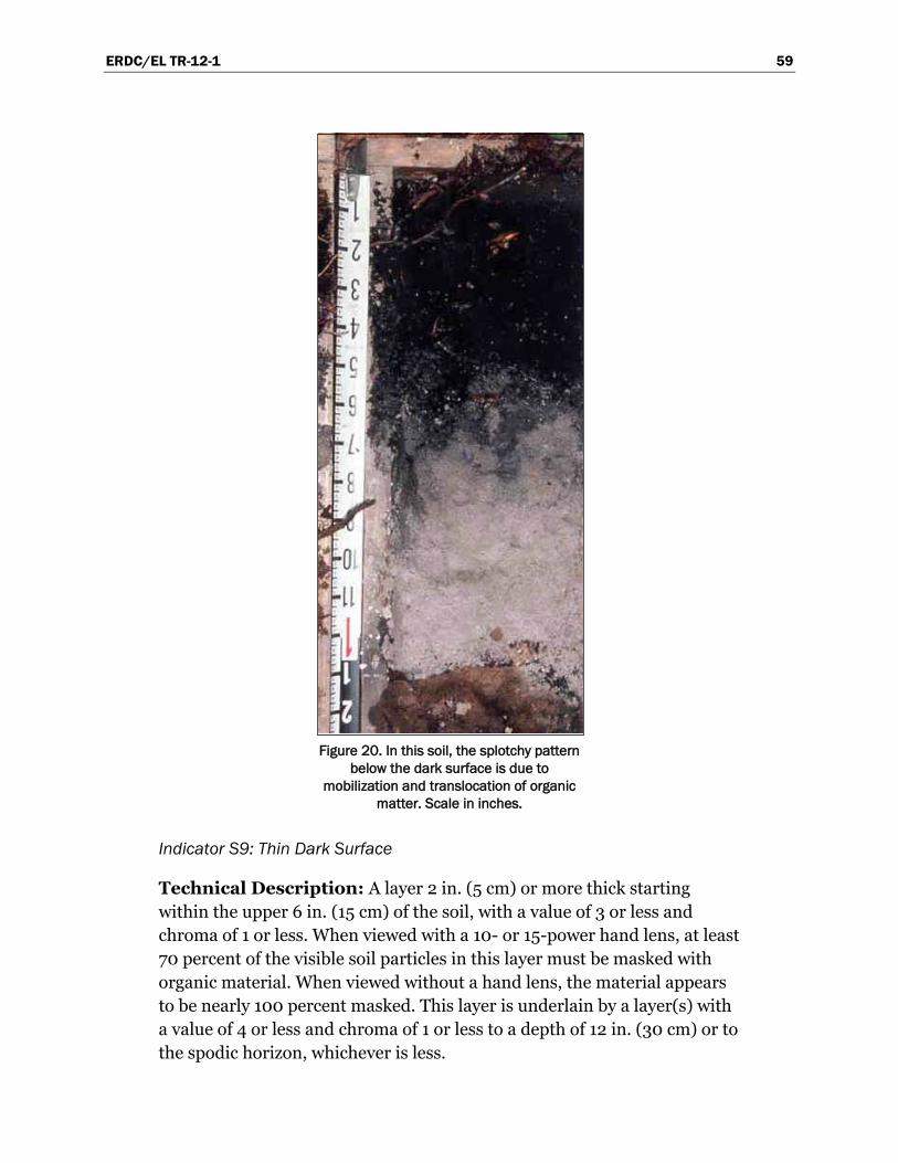
ERDC/EL TR-12-1 59
Figure 20. In this soil, the splotchy pattern
below the dark surface is due to mobilization and translocation of organic
matter. Scale in inches.
Indicator S9: Thin Dark Surface
Technical Description: A layer 2 in. (5 cm) or more thick starting within the upper 6 in. (15 cm) of the soil, with a value of 3 or less and chroma of 1 or less. When viewed with a 10- or 15-power hand lens, at least 70 percent of the visible soil particles in this layer must be masked with organic material. When viewed without a hand lens, the material appears to be nearly 100 percent masked. This layer is underlain by a layer(s) with a value of 4 or less and chroma of 1 or less to a depth of 12 in. (30 cm) or to the spodic horizon, whichever is less.
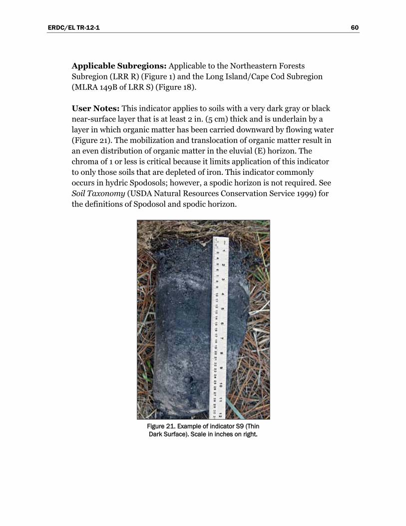
ERDC/EL TR-12-1 60
Applicable Subregions: Applicable to the Northeastern Forests Subregion (LRR R) (Figure 1) and the Long Island/Cape Cod Subregion (MLRA 149B of LRR S) (Figure 18).
User Notes: This indicator applies to soils with a very dark gray or black near-surface layer that is at least 2 in. (5 cm) thick and is underlain by a layer in which organic matter has been carried downward by flowing water (Figure 21). The mobilization and translocation of organic matter result in an even distribution of organic matter in the eluvial (E) horizon. The chroma of 1 or less is critical because it limits application of this indicator to only those soils that are depleted of iron. This indicator commonly occurs in hydric Spodosols; however, a spodic horizon is not required. See Soil Taxonomy (USDA Natural Resources Conservation Service 1999) for the definitions of Spodosol and spodic horizon.
Figure 21. Example of indicator S9 (Thin Dark Surface). Scale in inches on right.
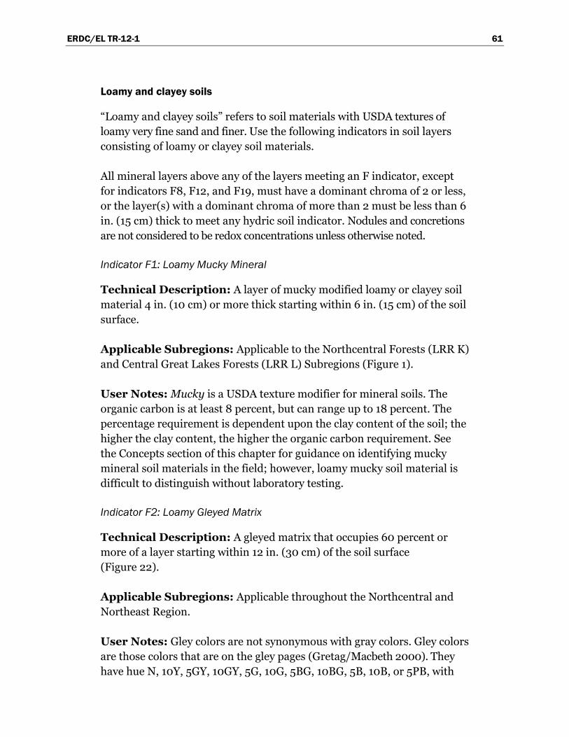
ERDC/EL TR-12-1 61
Loamy and clayey soils
“Loamy and clayey soils” refers to soil materials with USDA textures of loamy very fine sand and finer. Use the following indicators in soil layers consisting of loamy or clayey soil materials.
All mineral layers above any of the layers meeting an F indicator, except for indicators F8, F12, and F19, must have a dominant chroma of 2 or less, or the layer(s) with a dominant chroma of more than 2 must be less than 6 in. (15 cm) thick to meet any hydric soil indicator. Nodules and concretions are not considered to be redox concentrations unless otherwise noted.
Indicator F1: Loamy Mucky Mineral
Technical Description: A layer of mucky modified loamy or clayey soil material 4 in. (10 cm) or more thick starting within 6 in. (15 cm) of the soil surface.
Applicable Subregions: Applicable to the Northcentral Forests (LRR K) and Central Great Lakes Forests (LRR L) Subregions (Figure 1).
User Notes: Mucky is a USDA texture modifier for mineral soils. The organic carbon is at least 8 percent, but can range up to 18 percent. The percentage requirement is dependent upon the clay content of the soil; the higher the clay content, the higher the organic carbon requirement. See the Concepts section of this chapter for guidance on identifying mucky mineral soil materials in the field; however, loamy mucky soil material is difficult to distinguish without laboratory testing.
Indicator F2: Loamy Gleyed Matrix
Technical Description: A gleyed matrix that occupies 60 percent or more of a layer starting within 12 in. (30 cm) of the soil surface (Figure 22).
Applicable Subregions: Applicable throughout the Northcentral and Northeast Region.
User Notes: Gley colors are not synonymous with gray colors. Gley colors are those colors that are on the gley pages (Gretag/Macbeth 2000). They have hue N, 10Y, 5GY, 10GY, 5G, 10G, 5BG, 10BG, 5B, 10B, or 5PB, with
ERDC/EL TR-12-1 62
Figure 22. This soil has a gleyed matrix in the lowest layer, starting
about 7 in. (18 cm) from the soil surface. The layer above the gleyed matrix has a depleted matrix.
value 4 or more. The gleyed matrix only has to be present within 12 in. (30 cm) of the surface. Soils with gleyed matrices are saturated for signif-icant periods; therefore, no minimum thickness of gleyed layer is required. See the Glossary (Appendix A) for the definition of a gleyed matrix.
This indicator is found in soils that are inundated or saturated nearly all of the growing season in most years (e.g., in oxbows with permanent water) and is not usually found at the boundaries between wetlands and non-wetlands.
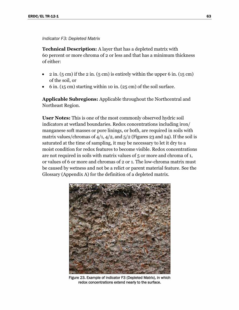
ERDC/EL TR-12-1 63
Indicator F3: Depleted Matrix
Technical Description: A layer that has a depleted matrix with 60 percent or more chroma of 2 or less and that has a minimum thickness of either:
• 2 in. (5 cm) if the 2 in. (5 cm) is entirely within the upper 6 in. (15 cm) of the soil, or
• 6 in. (15 cm) starting within 10 in. (25 cm) of the soil surface.
Applicable Subregions: Applicable throughout the Northcentral and Northeast Region.
User Notes: This is one of the most commonly observed hydric soil indicators at wetland boundaries. Redox concentrations including iron/ manganese soft masses or pore linings, or both, are required in soils with matrix values/chromas of 4/1, 4/2, and 5/2 (Figures 23 and 24). If the soil is saturated at the time of sampling, it may be necessary to let it dry to a moist condition for redox features to become visible. Redox concentrations are not required in soils with matrix values of 5 or more and chroma of 1, or values of 6 or more and chromas of 2 or 1. The low-chroma matrix must be caused by wetness and not be a relict or parent material feature. See the Glossary (Appendix A) for the definition of a depleted matrix.
Figure 23. Example of indicator F3 (Depleted Matrix), in which
redox concentrations extend nearly to the surface.
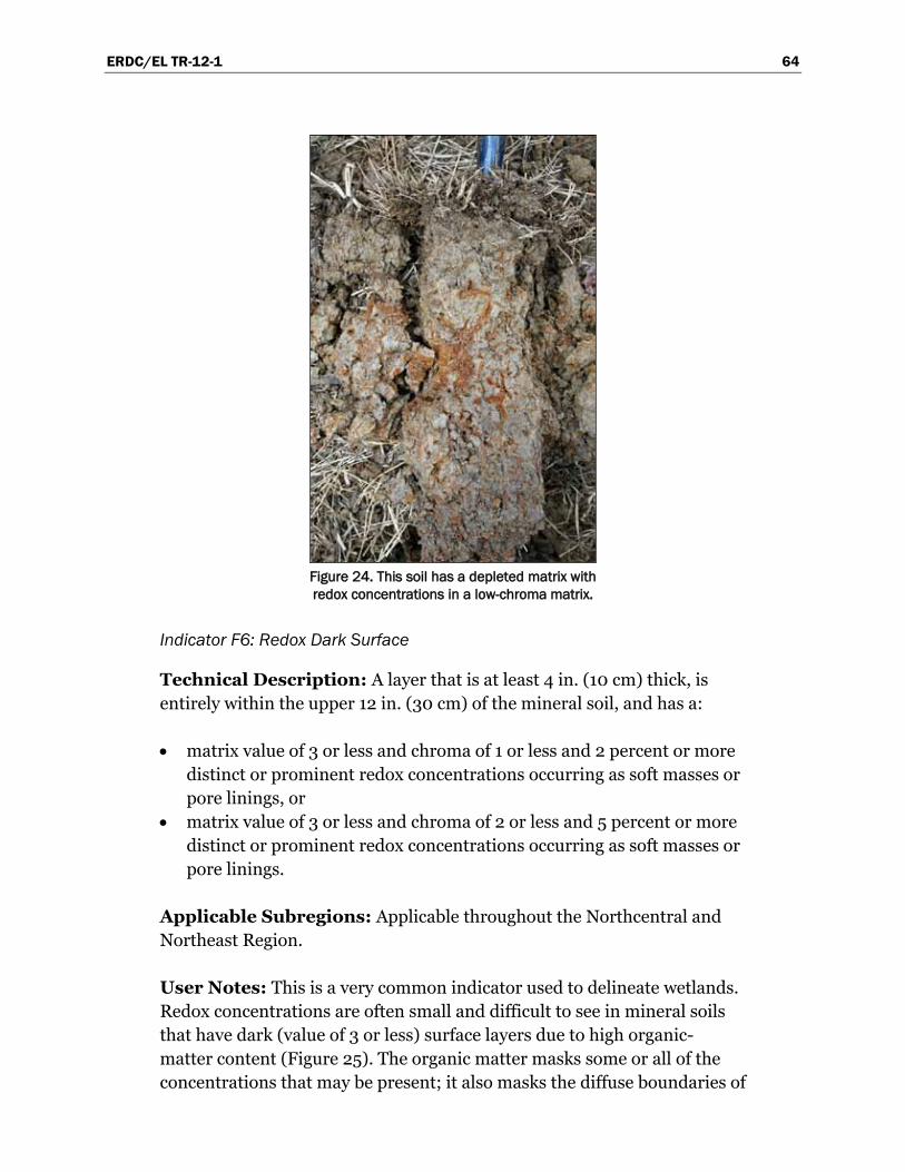
ERDC/EL TR-12-1 64
Figure 24. This soil has a depleted matrix with redox concentrations in a low-chroma matrix.
Indicator F6: Redox Dark Surface
Technical Description: A layer that is at least 4 in. (10 cm) thick, is entirely within the upper 12 in. (30 cm) of the mineral soil, and has a:
• matrix value of 3 or less and chroma of 1 or less and 2 percent or more distinct or prominent redox concentrations occurring as soft masses or pore linings, or
• matrix value of 3 or less and chroma of 2 or less and 5 percent or more distinct or prominent redox concentrations occurring as soft masses or pore linings.
Applicable Subregions: Applicable throughout the Northcentral and Northeast Region.
User Notes: This is a very common indicator used to delineate wetlands. Redox concentrations are often small and difficult to see in mineral soils that have dark (value of 3 or less) surface layers due to high organic-matter content (Figure 25). The organic matter masks some or all of the concentrations that may be present; it also masks the diffuse boundaries of
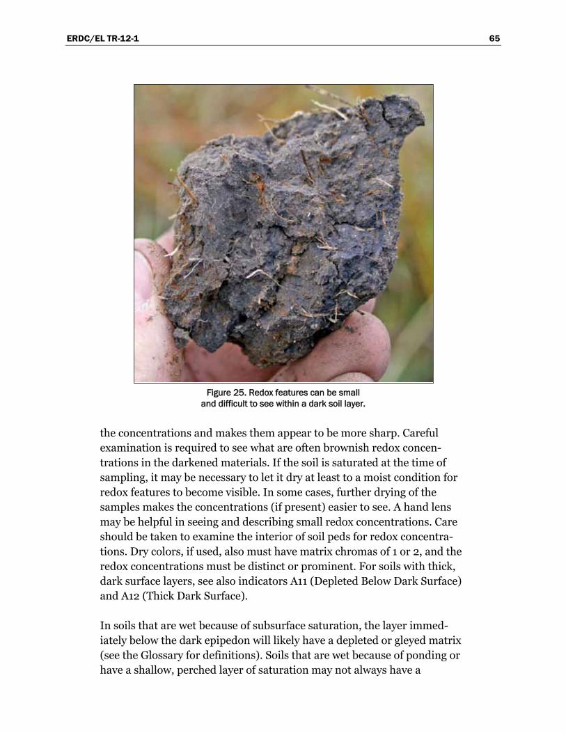
ERDC/EL TR-12-1 65
Figure 25. Redox features can be small
and difficult to see within a dark soil layer.
the concentrations and makes them appear to be more sharp. Careful examination is required to see what are often brownish redox concen-trations in the darkened materials. If the soil is saturated at the time of sampling, it may be necessary to let it dry at least to a moist condition for redox features to become visible. In some cases, further drying of the samples makes the concentrations (if present) easier to see. A hand lens may be helpful in seeing and describing small redox concentrations. Care should be taken to examine the interior of soil peds for redox concentra-tions. Dry colors, if used, also must have matrix chromas of 1 or 2, and the redox concentrations must be distinct or prominent. For soils with thick, dark surface layers, see also indicators A11 (Depleted Below Dark Surface) and A12 (Thick Dark Surface).
In soils that are wet because of subsurface saturation, the layer immed-iately below the dark epipedon will likely have a depleted or gleyed matrix (see the Glossary for definitions). Soils that are wet because of ponding or have a shallow, perched layer of saturation may not always have a
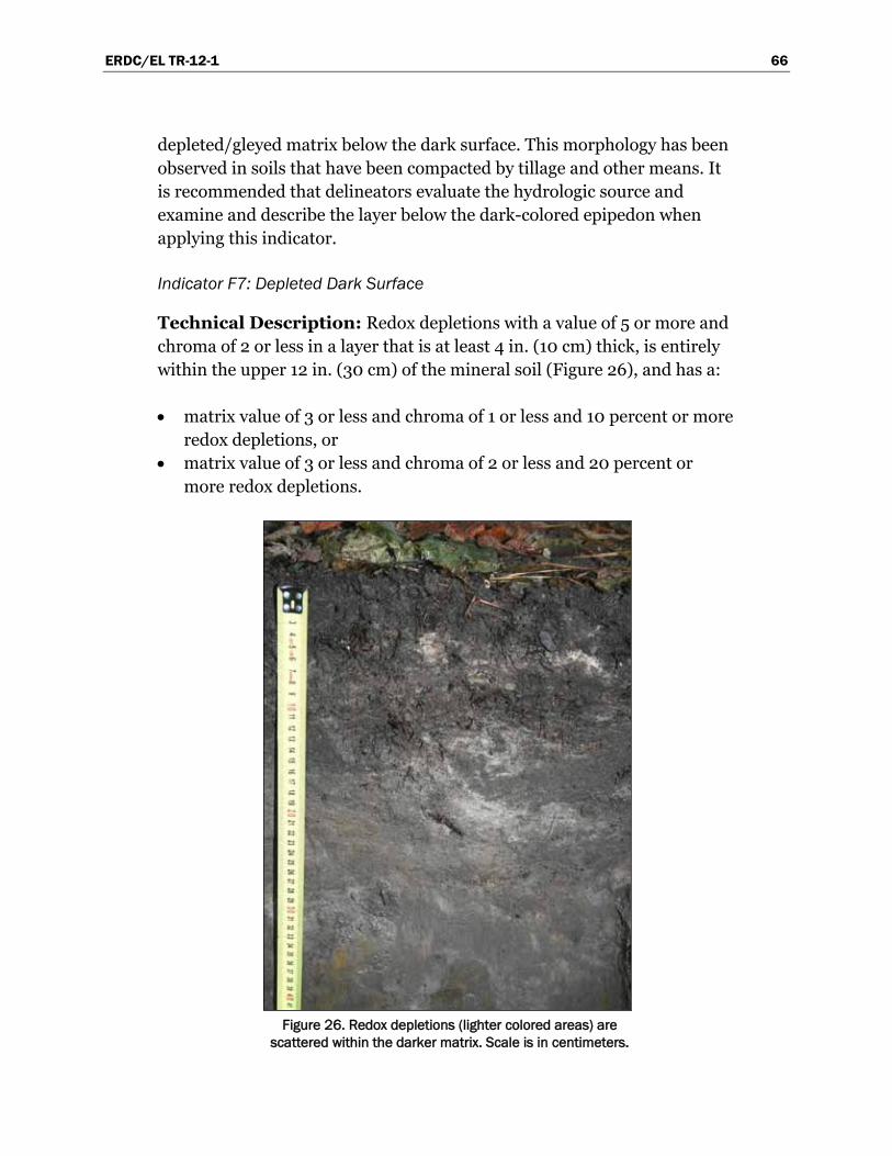
ERDC/EL TR-12-1 66
depleted/gleyed matrix below the dark surface. This morphology has been observed in soils that have been compacted by tillage and other means. It is recommended that delineators evaluate the hydrologic source and examine and describe the layer below the dark-colored epipedon when applying this indicator.
Indicator F7: Depleted Dark Surface
Technical Description: Redox depletions with a value of 5 or more and chroma of 2 or less in a layer that is at least 4 in. (10 cm) thick, is entirely within the upper 12 in. (30 cm) of the mineral soil (Figure 26), and has a:
• matrix value of 3 or less and chroma of 1 or less and 10 percent or more redox depletions, or
• matrix value of 3 or less and chroma of 2 or less and 20 percent or more redox depletions.
Figure 26. Redox depletions (lighter colored areas) are
scattered within the darker matrix. Scale is in centimeters.
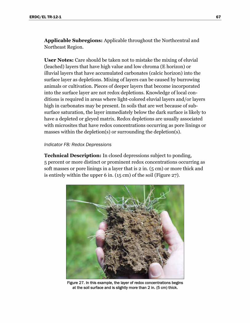
ERDC/EL TR-12-1 67
Applicable Subregions: Applicable throughout the Northcentral and Northeast Region.
User Notes: Care should be taken not to mistake the mixing of eluvial (leached) layers that have high value and low chroma (E horizon) or illuvial layers that have accumulated carbonates (calcic horizon) into the surface layer as depletions. Mixing of layers can be caused by burrowing animals or cultivation. Pieces of deeper layers that become incorporated into the surface layer are not redox depletions. Knowledge of local con-ditions is required in areas where light-colored eluvial layers and/or layers high in carbonates may be present. In soils that are wet because of sub-surface saturation, the layer immediately below the dark surface is likely to have a depleted or gleyed matrix. Redox depletions are usually associated with microsites that have redox concentrations occurring as pore linings or masses within the depletion(s) or surrounding the depletion(s).
Indicator F8: Redox Depressions
Technical Description: In closed depressions subject to ponding, 5 percent or more distinct or prominent redox concentrations occurring as soft masses or pore linings in a layer that is 2 in. (5 cm) or more thick and is entirely within the upper 6 in. (15 cm) of the soil (Figure 27).
Figure 27. In this example, the layer of redox concentrations begins
at the soil surface and is slightly more than 2 in. (5 cm) thick.
ERDC/EL TR-12-1 68
Applicable Subregions: Applicable throughout the Northcentral and Northeast Region.
User Notes: This indicator occurs on depressional landforms, such as vernal pools and potholes, but not microdepressions on convex land-scapes. Closed depressions often occur within flats or floodplain land-scapes. Note that there is no color requirement for the soil matrix. The layer containing redox concentrations may extend below 6 in. (15 cm) as long as at least 2 in. (5 cm) occurs within 6 in. (15 cm) of the surface. If the soil is saturated at the time of sampling, it may be necessary to let it dry to a moist condition for redox features to become visible. See the Glossary for definitions of distinct and prominent.
This is a common but often overlooked indicator found at the wetland/ non-wetland boundary on depressional sites.
Hydric soil indicators for problem soils
The following indicators are not currently recognized for general appli-cation by the NTCHS, or they are not recognized in the specified geo-graphic area. However, these indicators may be used in problem wetland situations in the Northcentral and Northeast Region where there is evi-dence of wetland hydrology and hydrophytic vegetation, and the soil is believed to meet the definition of a hydric soil despite the lack of other indicators of a hydric soil. To use these indicators, follow the procedure described in the section on Problematic Hydric Soils in Chapter 5. If any of the following indicators is observed, it is recommended that the NTCHS be notified by following the protocol described in the “Comment on the Indicators” section of Field Indicators of Hydric Soils in the United States (USDA Natural Resources Conservation Service 2010).
Indicator A10: 2 cm Muck
Technical Description: A layer of muck 0.75 in. (2 cm) or more thick with a value of 3 or less and chroma of 1 or less, starting within 6 in. (15 cm) of the soil surface.
Applicable Subregions: For use with problem soils in the Northcentral Forests (LRR K), Central Great Lakes Forests (LRR L), and Long Island/Cape Cod (MLRA 149B of LRR S) Subregions.
ERDC/EL TR-12-1 69
User Notes: Normally the muck layer is at the soil surface; however, it may occur at any depth within 6 in. (15 cm) of the surface. Muck is sapric soil material with at least 12 to 18 percent organic carbon. Organic soil material is called muck if virtually all of the material has undergone sufficient decomposition to limit recognition of the plant parts. Hemic (mucky peat) and fibric (peat) soil materials do not qualify. To determine if muck is present, first remove loose leaves, needles, bark, and other easily identified plant remains. This is sometimes called leaf litter, a duff layer, or a leaf or root mat. Then examine for decomposed organic soil material. Generally, muck is black and has a greasy feel; sand grains should not be evident (see the Concepts section of this chapter for field methods to identify organic soil materials). Determination of this indicator is made below the leaf or root mat; however, root mats that meet the definition of hemic or fibric soil material are included in the decision-making process for indicators A1 (Histosol) and A2 (Histic Epipedon).
Indicator A16: Coast Prairie Redox
Technical Description: A layer starting within 6 in. (15 cm) of the soil surface that is at least 4 in. (10 cm) thick and has a matrix chroma of 3 or less with 2 percent or more distinct or prominent redox concentrations occurring as soft masses and/or pore linings.
Applicable Subregions: For use with problem soils throughout the Northcentral and Northeast Region, except in the Long Island/Cape Cod Subregion (MLRA 149B of LRR S).
User Notes: These hydric soils occur mainly on depressional and intermound landforms. Redox concentrations occur mainly as iron-dominated pore linings. Common to many redox concentrations are required. If the soil is saturated at the time of sampling, it may be necessary to let it dry to a moist condition for redox features to become visible. Chroma 3 matrices are allowed because they may be the color of stripped sand grains, or because few to common sand-sized reddish particles may be present and may prevent obtaining a chroma of 2 or less.
Indicator S3: 5 cm Mucky Peat or Peat
Technical Description: A layer of mucky peat or peat 2 in. (5 cm) or more thick with a value of 3 or less and chroma of 2 or less, starting within 6 in. (15 cm) of the soil surface, and underlain by sandy soil material.
ERDC/EL TR-12-1 70
Applicable Subregions: For use with problem soils throughout the Northcentral and Northeast Region, except in the Long Island/Cape Cod Subregion (MLRA 149B of LRR S).
User Notes: In this region, this indicator is applicable primarily to interdunal swales along the Great Lakes and Atlantic coast. Mucky peat (hemic soil material) and peat (fibric soil material) have at least 12 to 18 percent organic carbon. Organic soil material is called peat if virtually all of the plant remains are sufficiently intact to permit identification of plant remains. Mucky peat is an intermediate stage of decomposition between peat and highly decomposed muck. See the glossary of Field Indicators of Hydric Soils in the United States (USDA Natural Resources Conservation Service 2010) for definitions. See the Concepts section of this chapter for field methods to identify organic soil materials.
Indicator S7: Dark Surface
Technical Description: A layer 4 in. (10 cm) thick starting within 6 in. (15 cm) of the soil surface with a matrix value of 3 or less and chroma of 1 or less. When viewed with a 10- or 15-power hand lens, at least 70 percent of the visible soil particles must be masked with organic material. When viewed without a hand lens, the material appears to be nearly 100 percent masked. The matrix color of the layer immediately below the dark layer must have the same colors as those described above or any color that has a chroma of 2 or less.
Applicable Subregions: For use with problem soils in the Northcentral Forests (LRR K) and Central Great Lakes Forests (LRR L) Subregions.
User Notes: This indicator is applicable to interdunal swales along the Great Lakes. See the User Notes for indicator S7 earlier in this chapter.
Indicator S8: Polyvalue Below Surface
Technical Description: A layer with a value of 3 or less and chroma of 1 or less starting within 6 in. (15 cm) of the soil surface. When viewed with a 10- or 15-power hand lens, at least 70 percent of the visible soil particles in this layer must be masked with organic material. When viewed without a hand lens, the material appears to be nearly 100 percent masked. Immediately below this layer, 5 percent or more of the soil volume has a value of 3 or less and chroma of 1 or less and the remainder of the soil
ERDC/EL TR-12-1 71
volume has a value of 4 or more and chroma of 1 or less to a depth of 12 in. (30 cm) or to the spodic horizon, whichever is less.
Applicable Subregions: For use with problem soils in the Northcentral Forests (LRR K) and Central Great Lakes Forests (LRR L) Subregions.
User Notes: See the User Notes for indicator S8 earlier in this chapter.
Indicator S9: Thin Dark Surface
Technical Description: A layer 2 in. (5 cm) or more thick starting within the upper 6 in. (15 cm) of the soil, with a value of 3 or less and chroma of 1 or less. When viewed with a 10- or 15-power hand lens, at least 70 percent of the visible soil particles in this layer must be masked with organic material. When viewed without a hand lens, the material appears to be nearly 100 percent masked. This layer is underlain by a layer(s) with a value of 4 or less and chroma of 1 or less to a depth of 12 in. (30 cm) or to the spodic horizon, whichever is less.
Applicable Subregions: For use with problem soils in the Northcentral Forests (LRR K) and Central Great Lakes Forests (LRR L) Subregions.
User Notes: See the User Notes for indicator S9 earlier in this chapter.
Indicator F12: Iron-Manganese Masses
Technical Description: On floodplains, a layer 4 in. (10 cm) or more thick with 40 percent or more chroma of 2 or less and 2 percent or more distinct or prominent redox concentrations occurring as soft iron-manganese masses with diffuse boundaries. The layer occurs entirely within 12 in. (30 cm) of the soil surface. Iron-manganese masses have a value and chroma of 3 or less. Most commonly, they are black. The thick-ness requirement is waived if the layer is the mineral surface layer.
Applicable Subregions: For use with problem soils throughout the Northcentral and Northeast Region, except in the Long Island/Cape Cod Subregion (MLRA 149B of LRR S).
User Notes: These iron-manganese masses generally are small (2 to 5 mm in size) and have value and chroma of 3 or less. They can be dominated by manganese and, therefore, have a color approaching black (Figure 28). If
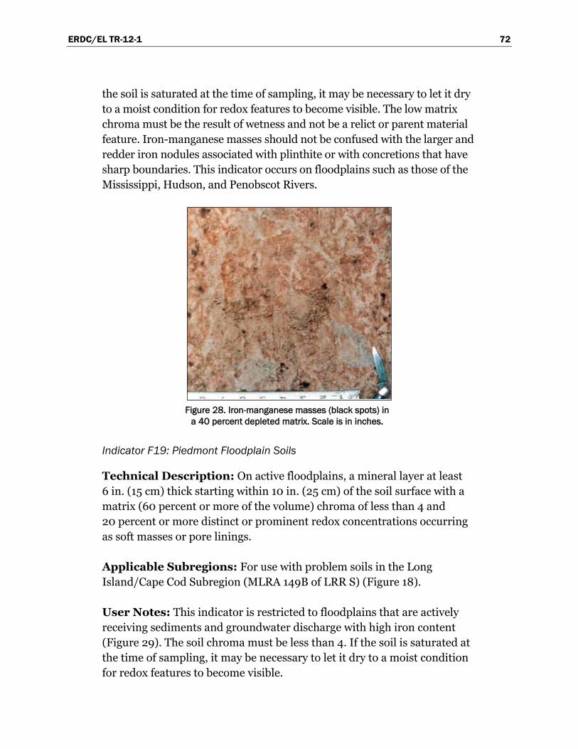
ERDC/EL TR-12-1 72
the soil is saturated at the time of sampling, it may be necessary to let it dry to a moist condition for redox features to become visible. The low matrix chroma must be the result of wetness and not be a relict or parent material feature. Iron-manganese masses should not be confused with the larger and redder iron nodules associated with plinthite or with concretions that have sharp boundaries. This indicator occurs on floodplains such as those of the Mississippi, Hudson, and Penobscot Rivers.
Figure 28. Iron-manganese masses (black spots) in
a 40 percent depleted matrix. Scale is in inches.
Indicator F19: Piedmont Floodplain Soils
Technical Description: On active floodplains, a mineral layer at least 6 in. (15 cm) thick starting within 10 in. (25 cm) of the soil surface with a matrix (60 percent or more of the volume) chroma of less than 4 and 20 percent or more distinct or prominent redox concentrations occurring as soft masses or pore linings.
Applicable Subregions: For use with problem soils in the Long Island/Cape Cod Subregion (MLRA 149B of LRR S) (Figure 18).
User Notes: This indicator is restricted to floodplains that are actively receiving sediments and groundwater discharge with high iron content (Figure 29). The soil chroma must be less than 4. If the soil is saturated at the time of sampling, it may be necessary to let it dry to a moist condition for redox features to become visible.
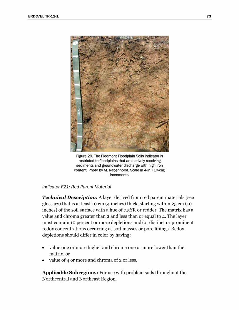
ERDC/EL TR-12-1 73
Figure 29. The Piedmont Floodplain Soils indicator is
restricted to floodplains that are actively receiving sediments and groundwater discharge with high iron
content. Photo by M. Rabenhorst. Scale in 4-in. (10-cm) increments.
Indicator F21: Red Parent Material
Technical Description: A layer derived from red parent materials (see glossary) that is at least 10 cm (4 inches) thick, starting within 25 cm (10 inches) of the soil surface with a hue of 7.5YR or redder. The matrix has a value and chroma greater than 2 and less than or equal to 4. The layer must contain 10 percent or more depletions and/or distinct or prominent redox concentrations occurring as soft masses or pore linings. Redox depletions should differ in color by having:
• value one or more higher and chroma one or more lower than the matrix, or
• value of 4 or more and chroma of 2 or less.
Applicable Subregions: For use with problem soils throughout the Northcentral and Northeast Region.
ERDC/EL TR-12-1 74
User Notes: This indicator was developed for use in areas of red parent material. In order to confirm that it is appropriate to apply this indicator to particular soils, soils formed from similar parent materials in the area should have been evaluated to determine their Color Change Propensity Index (CCPI) and be shown to have CCPI values below 30 (Rabenhorst and Parikh, 2000.) It cannot be assumed that sediment overlying red colored bedrock is derived solely from that bedrock. The total percentage of all redox concentrations and redox depletions must add up to at least 10% to meet the threshold for this indicator.
This indicator is typically found at the boundary between hydric and non-hydric soils. Users that encounter a depleted matrix in the upper part should consider F3-Depleted Matrix. F3 is often found in sites that are anaerobic for a longer period. Users that encounter a dark soil surface (value 3 or less and chroma 2 or less) should consider F6-Redox Dark Surface or F7-Depleted Dark Surface. If the site is in a closed depression subject to ponding users should consider F8-Redox Depressions. See glossary for definition of Red Parent Material.
Indicator TA6: Mesic Spodic
Technical Description: A layer 2 in. (5 cm) or more thick starting within 6 in. (15 cm) of the mineral soil surface that has a value of 3 or less and chroma of 2 or less and is underlain by either:
• a layer(s) 3 in. (8 cm) or more thick starting within 12 in. (30 cm) of the mineral soil surface that has a value and chroma of 3 or less and shows evidence of spodic development; or
• a layer(s) 2 in. (5 cm) or more thick starting within 12 in. (30 cm) of the mineral soil surface that has a value of 4 or more and chroma of 2 or less and is directly underlain by a layer(s) 3 in. (8 cm) or more thick with a value and chroma of 3 or less that shows evidence of spodic development.
Applicable Subregions: For use with problem soils in MLRAs 144A and 145 of LRR R and MLRA 149B of LRR S (Figure 30).
User Notes: This indicator is used to identify wet soils with spodic mate-rials or that meet the definition of a Spodosol in MLRAs 144A and 145 of LRR R and MLRA 149B of LRR S only. The layer that has a value of 4 or more and chroma of 2 or less is typically described as an E or Eg horizon. These typically have color patterns described as stripped or partially
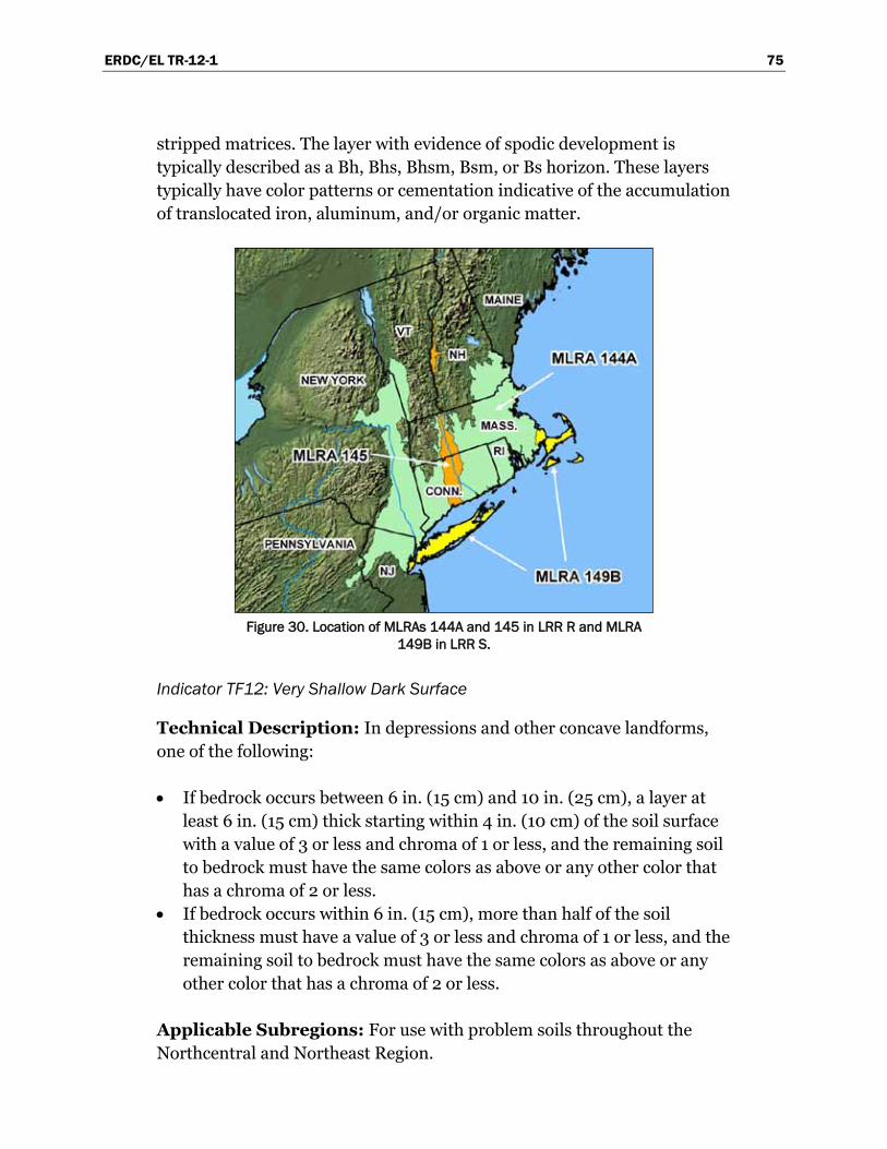
ERDC/EL TR-12-1 75
stripped matrices. The layer with evidence of spodic development is typically described as a Bh, Bhs, Bhsm, Bsm, or Bs horizon. These layers typically have color patterns or cementation indicative of the accumulation of translocated iron, aluminum, and/or organic matter.
Figure 30. Location of MLRAs 144A and 145 in LRR R and MLRA
149B in LRR S.
Indicator TF12: Very Shallow Dark Surface
Technical Description: In depressions and other concave landforms, one of the following:
• If bedrock occurs between 6 in. (15 cm) and 10 in. (25 cm), a layer at least 6 in. (15 cm) thick starting within 4 in. (10 cm) of the soil surface with a value of 3 or less and chroma of 1 or less, and the remaining soil to bedrock must have the same colors as above or any other color that has a chroma of 2 or less.
• If bedrock occurs within 6 in. (15 cm), more than half of the soil thickness must have a value of 3 or less and chroma of 1 or less, and the remaining soil to bedrock must have the same colors as above or any other color that has a chroma of 2 or less.
Applicable Subregions: For use with problem soils throughout the Northcentral and Northeast Region.
ERDC/EL TR-12-1 76
4 Wetland Hydrology Indicators Introduction
Wetland hydrology indicators are used in combination with indicators of hydric soil and hydrophytic vegetation to determine whether an area is a wetland under the Corps Manual. Indicators of hydrophytic vegetation and hydric soil generally reflect a site’s medium- to long-term wetness history. They provide readily observable evidence that episodes of inundation or soil saturation lasting more than a few days during the growing season have occurred repeatedly over a period of years and that the timing, duration, and frequency of wet conditions have been sufficient to produce a characteristic wetland plant community and hydric soil morphology. If hydrology has not been altered, vegetation and soils provide strong evidence that wetland hydrology is present (National Research Council 1995). Wetland hydrology indicators provide evidence that the site has a continuing wetland hydrologic regime and that hydric soils and hydrophytic vegetation are not relicts of a past hydrologic regime. Wetland hydrology indicators confirm that an episode of inundation or soil saturation occurred recently, but may provide little additional information about the timing, duration, or frequency of such events (National Research Council 1995).
Hydrology indicators are often the most transitory of wetland indicators. Some hydrology indicators are naturally temporary or seasonal, and many are affected by recent or long-term meteorological conditions. For example, indicators involving direct observation of surface water or saturated soils often are present only during the normal wet portion of the growing season and may be absent during the dry season or during drier-than-normal years. Hydrology indicators also may be subject to disturbance or destruct-tion by natural processes or human activities. Most wetlands in the Northcentral and Northeast Region will exhibit one or more of the hydro-logy indicators presented in this chapter. However, some wetlands may lack any of these indicators due to temporarily dry conditions, disturbance, or other factors. Therefore, the lack of an indicator is not evidence for the absence of wetland hydrology. See Chapter 5 (Difficult Wetland Situations in the Northcentral and Northeast Region) for help in identifying wetlands that may lack wetland hydrology indicators at certain times.

ERDC/EL TR-12-1 77
The Northcentral and Northeast Region has a humid, temperate climate with cold, snowy winters and moderate-to-abundant spring and summer rainfall in most areas and years. The dry season is less pronounced in this region than in the adjacent regions, but increased evapotranspiration during June, July, and August causes water tables to drop and surface water to recede from wetland margins. Particularly in seasonally saturated wetlands, hydrology indicators may be difficult to find during dry periods. On the other hand, some indicators may be present on non-wetland sites immediately after a heavy rain or during periods of unusually high precipi-tation, river stages, reservoir releases, runoff, or snowmelt. Therefore, it is important to consider weather and climatic conditions prior to the site visit to minimize both false-positive and false-negative wetland hydrology decisions. An understanding of normal seasonal and annual variations in rainfall, temperature, and other climatic conditions is important in inter-preting hydrology indicators in the region. Some useful sources of climatic data are described in Chapter 5.
Areas that have hydrophytic vegetation and hydric soils generally also have wetland hydrology unless the hydrologic regime has changed due to natural events or human activities (National Research Council 1995). Therefore, when wetland hydrology indicators are absent from an area that has indicators of hydric soil and hydrophytic vegetation, further information may be needed to determine whether or not wetland hydrology is present. If possible, one or more site visits should be scheduled to coincide with the normal wet portion of the growing season, the period of the year when the presence or absence of wetland hydrology indicators is most likely to reflect the true wetland/non-wetland status of the site. In addition, aerial photography or other remote-sensing data, stream gauge data, monitoring well data, runoff estimates, scope-and-effect equations for ditches and subsurface drainage systems, or groundwater modeling are tools that may help to determine whether wetland hydrology is present when indicators are equivocal or lacking (e.g., USDA Natural Resources Conservation Service 1997). Off-site procedures developed under the National Food Security Act Manual (USDA Natural Resources Conservation Service 1994), which use wetland mapping conventions developed by NRCS state offices, can help identify areas that have wetland hydrology on agricultural lands. The technique is based on wetness signatures visible on standard high-altitude aerial photographs or on annual crop-compliance slides taken by the USDA Farm Service Agency. Finally, on highly disturbed or problematic sites, direct hydrologic monitoring may be needed to determine whether wetland
ERDC/EL TR-12-1 78
hydrology is present. The U.S. Army Corps of Engineers (2005) provides a technical standard for monitoring hydrology on such sites. This standard requires 14 or more consecutive days of flooding, ponding, and/or a water table 12 in. (30 cm) or less below the soil surface, during the growing season, at a minimum frequency of 5 years in 10 (50 percent or higher probability) (National Research Council 1995) unless an alternative standard has been established for a particular region or wetland type. See Chapter 5 for further information on these techniques.
Growing season
Beginning and ending dates of the growing season may be needed to evaluate certain wetland indicators, such as visual observations of flood-ing, ponding, or shallow water tables on potential wetland sites. In addi-tion, growing season dates are needed in the event that recorded hydro-logic data, such as stream gauge or water-table monitoring data, must be analyzed to determine whether wetland hydrology is present on highly disturbed or problematic sites.
Depletion of oxygen and the chemical reduction of nitrogen, iron, and other elements in saturated soils during the growing season is the result of biological activity occurring in plant roots and soil microbial populations (National Research Council 1995). Two indicators of biological activity that are readily observable in the field are (1) above-ground growth and devel-opment of vascular plants, and (2) soil temperature as an indicator of soil microbial activity (Megonigal et al. 1996, USDA Natural Resources Con-servation Service 1999). If information about growing season is needed and on-site data gathering is practical, the following approaches should be used in this region to determine growing season dates in a given year. The growing season has begun and is ongoing if either of these conditions is met. Therefore, the beginning of the growing season in a given year is indicated by whichever condition occurs earlier, and the end of the grow-ing season is indicated by whichever condition persists later.
1. The growing season has begun on a site in a given year when two or more different non-evergreen vascular plant species growing in the wetland or surrounding areas exhibit one or more of the following indicators of biological activity:
a. Emergence of herbaceous plants from the ground
ERDC/EL TR-12-1 79
b. Appearance of new growth from vegetative crowns (e.g., in graminoids, bulbs, and corms)
c. Coleoptile/cotyledon emergence from seed d. Bud burst on woody plants (i.e., some green foliage is visible between
spreading bud scales) e. Emergence or elongation of leaves of woody plants f. Emergence or opening of flowers
The end of the growing season is indicated when woody deciduous species lose their leaves or the last herbaceous plants cease flowering and their leaves become dry or brown, whichever occurs latest. These changes generally take place in the fall due to cold temperatures or reduced moisture availability. Early plant senescence due to the initi-ation of the summer dry season in some areas does not necessarily indicate the end of the growing season and alternative procedures (e.g., soil temperature) should be used.
Determinations of the beginning or the end of the growing season should not include evergreen species, including such herbaceous species as Polystichum acrostichoides and Lycopodium spp. or deciduous species that retain their leaves into the winter (e.g., Rhamnus cathartica). Certain herbaceous plants, such as Alliaria petiolata, Carex blanda, Geum canadense, and Hesperis matronalis, have basal rosettes and lower stem leaves that retain chlorophyll and remain green throughout the year, including winter (Figure 31). The winter presence of green tissue in these species is not considered a vegetative signal that the growing season has begun. These types of herbaceous species do not indicate the beginning or end of the growing season. If limited to using these types of species, look for new growth from the vegetative crowns to meet the biological activity indicator.
Observations should be made in the wetland or in surrounding areas subject to the same climatic conditions (e.g., similar elevation and aspect); however, soil moisture conditions and plant communities may differ. Supporting data should be reported on the data form, in field notes, or in the delineation report, and should include the species observed (if identifiable), their abundance and location relative to the potential wetland, and type of biological activity observed. A one-time observation of biological activity during a single site visit is sufficient,
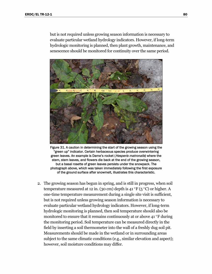
ERDC/EL TR-12-1 80
but is not required unless growing season information is necessary to evaluate particular wetland hydrology indicators. However, if long-term hydrologic monitoring is planned, then plant growth, maintenance, and senescence should be monitored for continuity over the same period.
Figure 31. A caution in determining the start of the growing season using the
“green up” indicator. Certain herbaceous species produce overwintering green leaves. An example is Dame’s rocket (Hesperis matronalis) where the stem, stem leaves, and flowers die back at the end of the growing season,
but a basal rosette of green leaves persists under the snowpack. The photograph above, which was taken immediately following the first exposure
of the ground surface after snowmelt, illustrates this characteristic.
2. The growing season has begun in spring, and is still in progress, when soil temperature measured at 12 in. (30 cm) depth is 41 °F (5 °C) or higher. A one-time temperature measurement during a single site visit is sufficient, but is not required unless growing season information is necessary to evaluate particular wetland hydrology indicators. However, if long-term hydrologic monitoring is planned, then soil temperature should also be monitored to ensure that it remains continuously at or above 41 °F during the monitoring period. Soil temperature can be measured directly in the field by inserting a soil thermometer into the wall of a freshly dug soil pit. Measurements should be made in the wetland or in surrounding areas subject to the same climatic conditions (e.g., similar elevation and aspect); however, soil moisture conditions may differ.
ERDC/EL TR-12-1 81
If the timing of the growing season based on vegetation growth and development and/or soil temperature is unknown and on-site data collection is not practical, such as when analyzing previously recorded stream-gauge or monitoring-well data, then growing season dates may be approximated by the median dates (i.e., 5 years in 10, or 50 percent prob-ability) of 28 °F (−2.2 °C) air temperatures in spring and fall, based on long-term records gathered at National Weather Service meteorological stations (U.S. Army Corps of Engineers 2005). These dates are reported in WETS tables available from the NRCS National Water and Climate Center (http://www.wcc.nrcs.usda.gov/climate/wetlands.html) for the nearest appropriate weather station.
Wetland hydrology indicators
In this chapter, wetland hydrology indicators are presented in four groups. Indicators in Group A are based on the direct observation of surface water or groundwater during a site visit. Group B consists of evidence that the site is subject to flooding or ponding, although it may not be inundated currently. These indicators include water marks, drift deposits, sediment deposits, and similar features. Group C consists of other evidence that the soil is saturated currently or was saturated recently (e.g., oxidized rhizo-spheres surrounding living roots and the presence of reduced iron or sulfur in the soil profile). Group D consists of landscape, soil, and vege-tation features that indicate contemporary rather than historical wet conditions. Wetland hydrology indicators are intended as one-time observations of site conditions that are sufficient evidence of wetland hydrology. Unless otherwise noted, all indicators are applicable throughout the Northcentral and Northeast Region.
Within each group, indicators are divided into two categories – primary and secondary – based on their estimated reliability in this region. One primary indicator from any group is sufficient to conclude that wetland hydrology is present; the area is a wetland if indicators of hydric soil and hydrophytic vegetation are also present. In the absence of a primary indi-cator, two or more secondary indicators from any group are required to conclude that wetland hydrology is present. Indicators of wetland hydrol-ogy include, but are not necessarily limited to, those listed in Table 10 and described on the following pages. Other evidence of wetland hydrology may also be used with appropriate documentation.
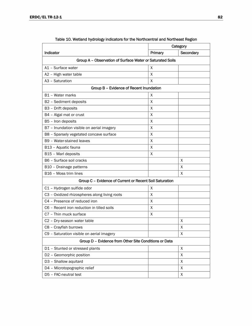
ERDC/EL TR-12-1 82
Table 10. Wetland hydrology indicators for the Northcentral and Northeast Region
Indicator Category
Primary Secondary
Group A – Observation of Surface Water or Saturated Soils
A1 – Surface water X A2 – High water table X A3 – Saturation X
Group B – Evidence of Recent Inundation
B1 – Water marks X B2 – Sediment deposits X B3 – Drift deposits X B4 – Algal mat or crust X B5 – Iron deposits X B7 – Inundation visible on aerial imagery X B8 – Sparsely vegetated concave surface X B9 – Water-stained leaves X B13 – Aquatic fauna X B15 – Marl deposits X B6 – Surface soil cracks X B10 – Drainage patterns X B16 – Moss trim lines X
Group C – Evidence of Current or Recent Soil Saturation
C1 – Hydrogen sulfide odor X C3 – Oxidized rhizospheres along living roots X C4 – Presence of reduced iron X C6 – Recent iron reduction in tilled soils X C7 – Thin muck surface X C2 – Dry-season water table X C8 – Crayfish burrows X C9 – Saturation visible on aerial imagery X
Group D – Evidence from Other Site Conditions or Data
D1 – Stunted or stressed plants X D2 – Geomorphic position X D3 – Shallow aquitard X D4 – Microtopographic relief X D5 – FAC-neutral test X
ERDC/EL TR-12-1 83
In this supplement, wetland hydrology indicators that have depth require-ments (e.g., indicator A2 – High Water Table) are evaluated from the mineral soil surface or the top of any organic soil layer, whichever is shallower. Organic layers consist of dead and decomposing plant matter. Therefore, observations should start below any living material (e.g., a living mat of mosses, lichens, etc.). The organic layer, if present, can be either saturated or unsaturated and of any thickness. Therefore, on some sites, the surface for hydric soil determinations (see Chapter 3) and wet-land hydrology determinations may differ.
Group A – Observation of Surface Water or Saturated Soils
Indicator A1: Surface water
Category: Primary
General Description: This indicator consists of the direct, visual obser-vation of surface water (flooding or ponding) during a site visit (Figure 32).
Cautions and User Notes: Care must be used in applying this indicator because surface water may be present in non-wetland areas immediately after a rainfall event or during periods of unusually high precipitation, runoff, tides, or river stages. Furthermore, some non-wetlands flood fre-quently for brief periods. Surface water observed during the non-growing season may be an acceptable indicator if experience and professional judgment suggest that wet conditions normally extend into the growing season for sufficient duration in most years. If this is questionable and other hydrology indicators are absent, a follow-up visit during the growing season may be needed. Water perched on seasonally frozen soil is included in this indicator if the resulting inundation is normally present well into the growing season. Note that surface water may be absent from a wetland during the normal dry season or during extended periods of drought. Even under normal rainfall conditions, some wetlands do not become inundated or saturated every year (i.e., wetlands are inundated or saturated at least 5 out of 10 years, or 50 percent or higher probability). In addition, groundwater-dominated wetland systems may never or rarely contain surface water.
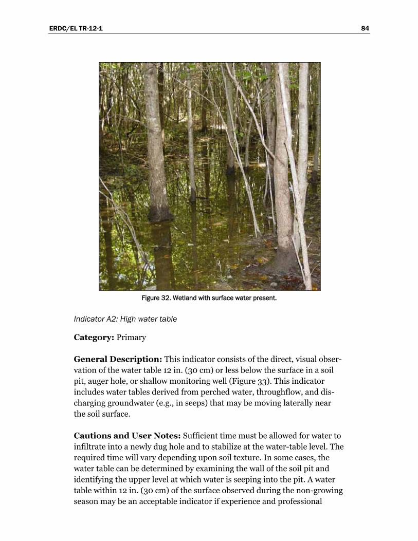
ERDC/EL TR-12-1 84
Figure 32. Wetland with surface water present.
Indicator A2: High water table
Category: Primary
General Description: This indicator consists of the direct, visual obser-vation of the water table 12 in. (30 cm) or less below the surface in a soil pit, auger hole, or shallow monitoring well (Figure 33). This indicator includes water tables derived from perched water, throughflow, and dis-charging groundwater (e.g., in seeps) that may be moving laterally near the soil surface.
Cautions and User Notes: Sufficient time must be allowed for water to infiltrate into a newly dug hole and to stabilize at the water-table level. The required time will vary depending upon soil texture. In some cases, the water table can be determined by examining the wall of the soil pit and identifying the upper level at which water is seeping into the pit. A water table within 12 in. (30 cm) of the surface observed during the non-growing season may be an acceptable indicator if experience and professional
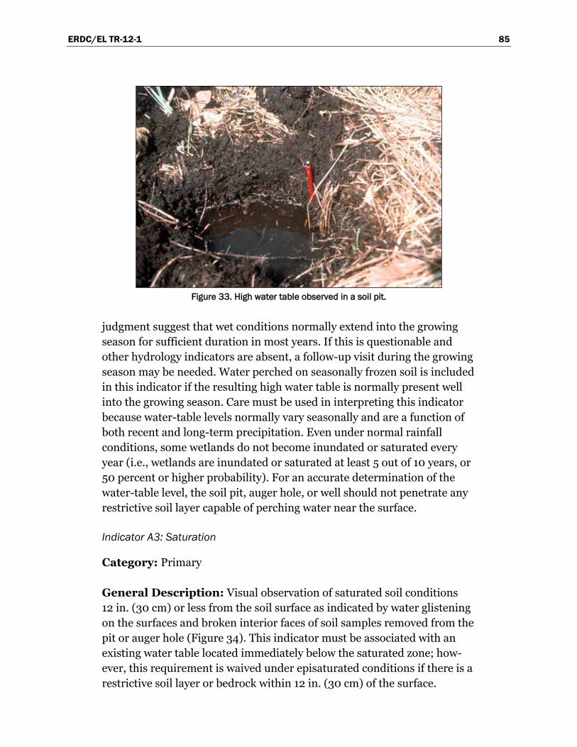
ERDC/EL TR-12-1 85
Figure 33. High water table observed in a soil pit.
judgment suggest that wet conditions normally extend into the growing season for sufficient duration in most years. If this is questionable and other hydrology indicators are absent, a follow-up visit during the growing season may be needed. Water perched on seasonally frozen soil is included in this indicator if the resulting high water table is normally present well into the growing season. Care must be used in interpreting this indicator because water-table levels normally vary seasonally and are a function of both recent and long-term precipitation. Even under normal rainfall conditions, some wetlands do not become inundated or saturated every year (i.e., wetlands are inundated or saturated at least 5 out of 10 years, or 50 percent or higher probability). For an accurate determination of the water-table level, the soil pit, auger hole, or well should not penetrate any restrictive soil layer capable of perching water near the surface.
Indicator A3: Saturation
Category: Primary
General Description: Visual observation of saturated soil conditions 12 in. (30 cm) or less from the soil surface as indicated by water glistening on the surfaces and broken interior faces of soil samples removed from the pit or auger hole (Figure 34). This indicator must be associated with an existing water table located immediately below the saturated zone; how-ever, this requirement is waived under episaturated conditions if there is a restrictive soil layer or bedrock within 12 in. (30 cm) of the surface.
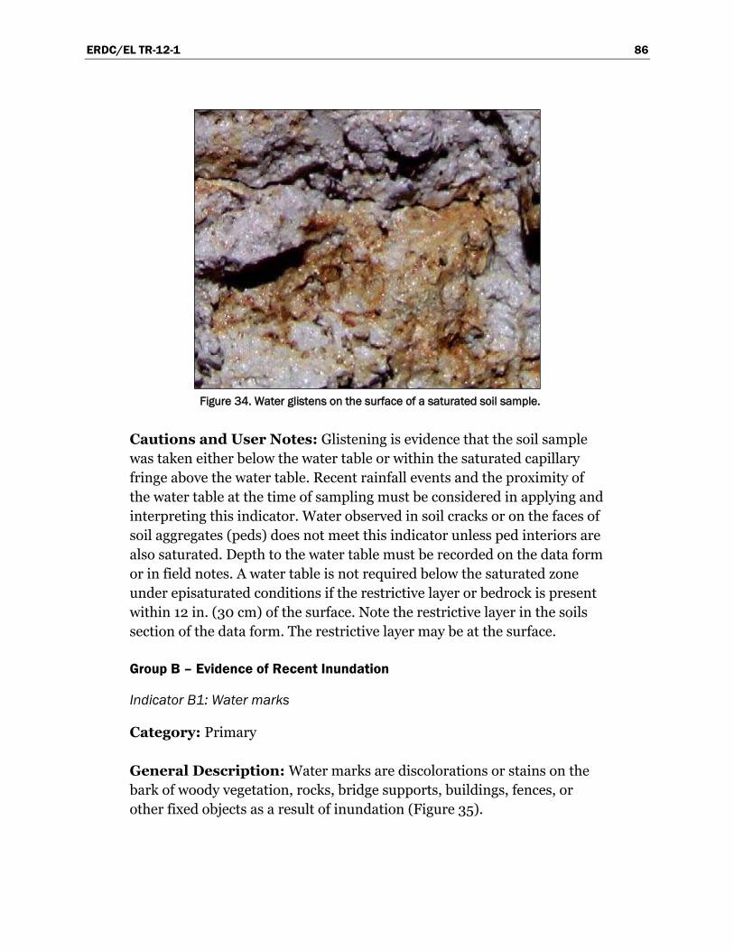
ERDC/EL TR-12-1 86
Figure 34. Water glistens on the surface of a saturated soil sample.
Cautions and User Notes: Glistening is evidence that the soil sample was taken either below the water table or within the saturated capillary fringe above the water table. Recent rainfall events and the proximity of the water table at the time of sampling must be considered in applying and interpreting this indicator. Water observed in soil cracks or on the faces of soil aggregates (peds) does not meet this indicator unless ped interiors are also saturated. Depth to the water table must be recorded on the data form or in field notes. A water table is not required below the saturated zone under episaturated conditions if the restrictive layer or bedrock is present within 12 in. (30 cm) of the surface. Note the restrictive layer in the soils section of the data form. The restrictive layer may be at the surface.
Group B – Evidence of Recent Inundation
Indicator B1: Water marks
Category: Primary
General Description: Water marks are discolorations or stains on the bark of woody vegetation, rocks, bridge supports, buildings, fences, or other fixed objects as a result of inundation (Figure 35).
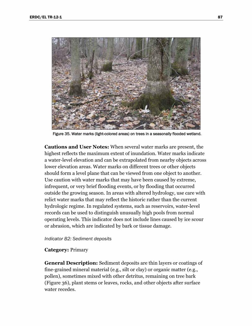
ERDC/EL TR-12-1 87
Figure 35. Water marks (light-colored areas) on trees in a seasonally flooded wetland.
Cautions and User Notes: When several water marks are present, the highest reflects the maximum extent of inundation. Water marks indicate a water-level elevation and can be extrapolated from nearby objects across lower elevation areas. Water marks on different trees or other objects should form a level plane that can be viewed from one object to another. Use caution with water marks that may have been caused by extreme, infrequent, or very brief flooding events, or by flooding that occurred outside the growing season. In areas with altered hydrology, use care with relict water marks that may reflect the historic rather than the current hydrologic regime. In regulated systems, such as reservoirs, water-level records can be used to distinguish unusually high pools from normal operating levels. This indicator does not include lines caused by ice scour or abrasion, which are indicated by bark or tissue damage.
Indicator B2: Sediment deposits
Category: Primary
General Description: Sediment deposits are thin layers or coatings of fine-grained mineral material (e.g., silt or clay) or organic matter (e.g., pollen), sometimes mixed with other detritus, remaining on tree bark (Figure 36), plant stems or leaves, rocks, and other objects after surface water recedes.
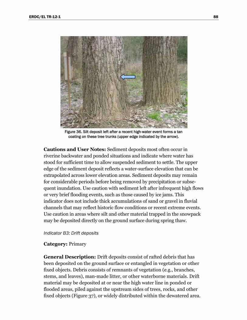
ERDC/EL TR-12-1 88
Figure 36. Silt deposit left after a recent high-water event forms a tan
coating on these tree trunks (upper edge indicated by the arrow).
Cautions and User Notes: Sediment deposits most often occur in riverine backwater and ponded situations and indicate where water has stood for sufficient time to allow suspended sediment to settle. The upper edge of the sediment deposit reflects a water-surface elevation that can be extrapolated across lower elevation areas. Sediment deposits may remain for considerable periods before being removed by precipitation or subse-quent inundation. Use caution with sediment left after infrequent high flows or very brief flooding events, such as those caused by ice jams. This indicator does not include thick accumulations of sand or gravel in fluvial channels that may reflect historic flow conditions or recent extreme events. Use caution in areas where silt and other material trapped in the snowpack may be deposited directly on the ground surface during spring thaw.
Indicator B3: Drift deposits
Category: Primary
General Description: Drift deposits consist of rafted debris that has been deposited on the ground surface or entangled in vegetation or other fixed objects. Debris consists of remnants of vegetation (e.g., branches, stems, and leaves), man-made litter, or other waterborne materials. Drift material may be deposited at or near the high water line in ponded or flooded areas, piled against the upstream sides of trees, rocks, and other fixed objects (Figure 37), or widely distributed within the dewatered area.
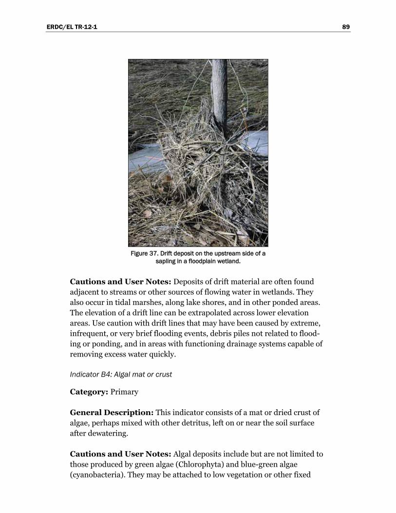
ERDC/EL TR-12-1 89
Figure 37. Drift deposit on the upstream side of a
sapling in a floodplain wetland.
Cautions and User Notes: Deposits of drift material are often found adjacent to streams or other sources of flowing water in wetlands. They also occur in tidal marshes, along lake shores, and in other ponded areas. The elevation of a drift line can be extrapolated across lower elevation areas. Use caution with drift lines that may have been caused by extreme, infrequent, or very brief flooding events, debris piles not related to flood-ing or ponding, and in areas with functioning drainage systems capable of removing excess water quickly.
Indicator B4: Algal mat or crust
Category: Primary
General Description: This indicator consists of a mat or dried crust of algae, perhaps mixed with other detritus, left on or near the soil surface after dewatering.
Cautions and User Notes: Algal deposits include but are not limited to those produced by green algae (Chlorophyta) and blue-green algae (cyanobacteria). They may be attached to low vegetation or other fixed
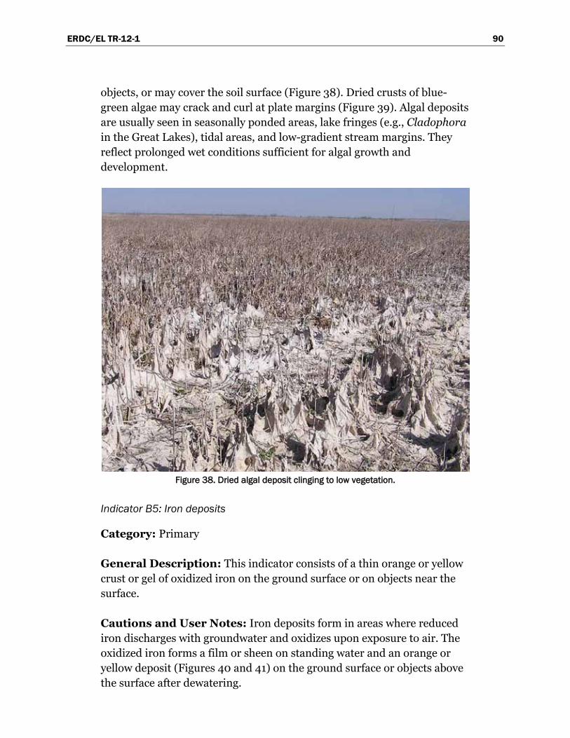
ERDC/EL TR-12-1 90
objects, or may cover the soil surface (Figure 38). Dried crusts of blue-green algae may crack and curl at plate margins (Figure 39). Algal deposits are usually seen in seasonally ponded areas, lake fringes (e.g., Cladophora in the Great Lakes), tidal areas, and low-gradient stream margins. They reflect prolonged wet conditions sufficient for algal growth and development.
Figure 38. Dried algal deposit clinging to low vegetation.
Indicator B5: Iron deposits
Category: Primary
General Description: This indicator consists of a thin orange or yellow crust or gel of oxidized iron on the ground surface or on objects near the surface.
Cautions and User Notes: Iron deposits form in areas where reduced iron discharges with groundwater and oxidizes upon exposure to air. The oxidized iron forms a film or sheen on standing water and an orange or yellow deposit (Figures 40 and 41) on the ground surface or objects above the surface after dewatering.
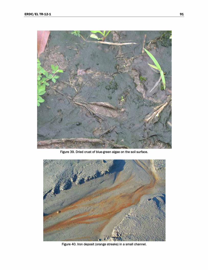
ERDC/EL TR-12-1 91
Figure 39. Dried crust of blue-green algae on the soil surface.
Figure 40. Iron deposit (orange streaks) in a small channel.
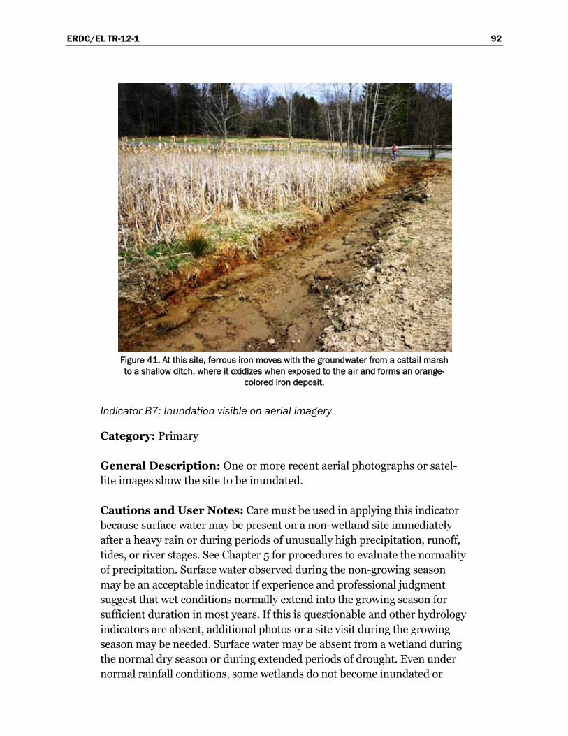
ERDC/EL TR-12-1 92
Figure 41. At this site, ferrous iron moves with the groundwater from a cattail marsh to a shallow ditch, where it oxidizes when exposed to the air and forms an orange-
colored iron deposit.
Indicator B7: Inundation visible on aerial imagery
Category: Primary
General Description: One or more recent aerial photographs or satel-lite images show the site to be inundated.
Cautions and User Notes: Care must be used in applying this indicator because surface water may be present on a non-wetland site immediately after a heavy rain or during periods of unusually high precipitation, runoff, tides, or river stages. See Chapter 5 for procedures to evaluate the normality of precipitation. Surface water observed during the non-growing season may be an acceptable indicator if experience and professional judgment suggest that wet conditions normally extend into the growing season for sufficient duration in most years. If this is questionable and other hydrology indicators are absent, additional photos or a site visit during the growing season may be needed. Surface water may be absent from a wetland during the normal dry season or during extended periods of drought. Even under normal rainfall conditions, some wetlands do not become inundated or
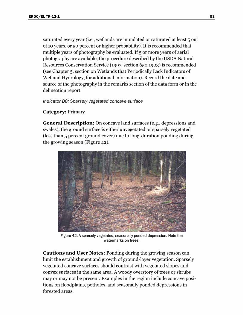
ERDC/EL TR-12-1 93
saturated every year (i.e., wetlands are inundated or saturated at least 5 out of 10 years, or 50 percent or higher probability). It is recommended that multiple years of photography be evaluated. If 5 or more years of aerial photography are available, the procedure described by the USDA Natural Resources Conservation Service (1997, section 650.1903) is recommended (see Chapter 5, section on Wetlands that Periodically Lack Indicators of Wetland Hydrology, for additional information). Record the date and source of the photography in the remarks section of the data form or in the delineation report.
Indicator B8: Sparsely vegetated concave surface
Category: Primary
General Description: On concave land surfaces (e.g., depressions and swales), the ground surface is either unvegetated or sparsely vegetated (less than 5 percent ground cover) due to long-duration ponding during the growing season (Figure 42).
Figure 42. A sparsely vegetated, seasonally ponded depression. Note the
watermarks on trees.
Cautions and User Notes: Ponding during the growing season can limit the establishment and growth of ground-layer vegetation. Sparsely vegetated concave surfaces should contrast with vegetated slopes and convex surfaces in the same area. A woody overstory of trees or shrubs may or may not be present. Examples in the region include concave posi-tions on floodplains, potholes, and seasonally ponded depressions in forested areas.
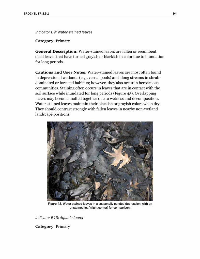
ERDC/EL TR-12-1 94
Indicator B9: Water-stained leaves
Category: Primary
General Description: Water-stained leaves are fallen or recumbent dead leaves that have turned grayish or blackish in color due to inundation for long periods.
Cautions and User Notes: Water-stained leaves are most often found in depressional wetlands (e.g., vernal pools) and along streams in shrub-dominated or forested habitats; however, they also occur in herbaceous communities. Staining often occurs in leaves that are in contact with the soil surface while inundated for long periods (Figure 43). Overlapping leaves may become matted together due to wetness and decomposition. Water-stained leaves maintain their blackish or grayish colors when dry. They should contrast strongly with fallen leaves in nearby non-wetland landscape positions.
Figure 43. Water-stained leaves in a seasonally ponded depression, with an
unstained leaf (right center) for comparison.
Indicator B13: Aquatic fauna
Category: Primary
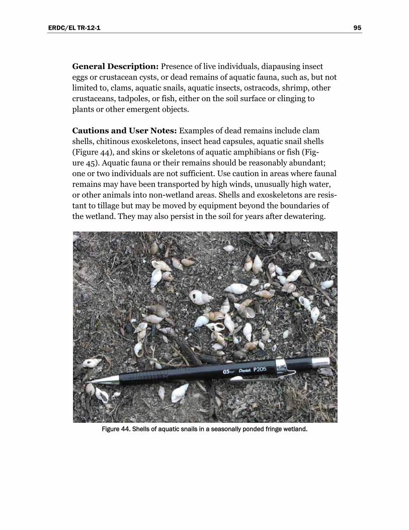
ERDC/EL TR-12-1 95
General Description: Presence of live individuals, diapausing insect eggs or crustacean cysts, or dead remains of aquatic fauna, such as, but not limited to, clams, aquatic snails, aquatic insects, ostracods, shrimp, other crustaceans, tadpoles, or fish, either on the soil surface or clinging to plants or other emergent objects.
Cautions and User Notes: Examples of dead remains include clam shells, chitinous exoskeletons, insect head capsules, aquatic snail shells (Figure 44), and skins or skeletons of aquatic amphibians or fish (Fig-ure 45). Aquatic fauna or their remains should be reasonably abundant; one or two individuals are not sufficient. Use caution in areas where faunal remains may have been transported by high winds, unusually high water, or other animals into non-wetland areas. Shells and exoskeletons are resis-tant to tillage but may be moved by equipment beyond the boundaries of the wetland. They may also persist in the soil for years after dewatering.
Figure 44. Shells of aquatic snails in a seasonally ponded fringe wetland.
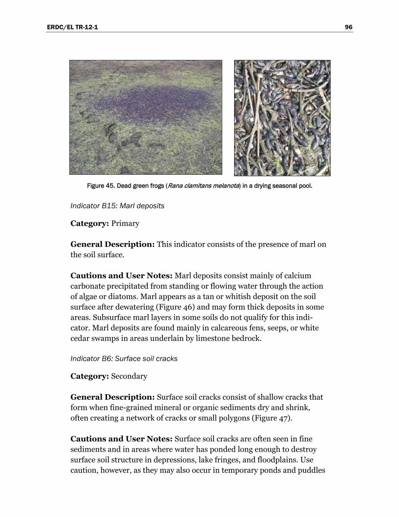
ERDC/EL TR-12-1 96
Figure 45. Dead green frogs (Rana clamitans melanota) in a drying seasonal pool.
Indicator B15: Marl deposits
Category: Primary
General Description: This indicator consists of the presence of marl on the soil surface.
Cautions and User Notes: Marl deposits consist mainly of calcium carbonate precipitated from standing or flowing water through the action of algae or diatoms. Marl appears as a tan or whitish deposit on the soil surface after dewatering (Figure 46) and may form thick deposits in some areas. Subsurface marl layers in some soils do not qualify for this indi-cator. Marl deposits are found mainly in calcareous fens, seeps, or white cedar swamps in areas underlain by limestone bedrock.
Indicator B6: Surface soil cracks
Category: Secondary
General Description: Surface soil cracks consist of shallow cracks that form when fine-grained mineral or organic sediments dry and shrink, often creating a network of cracks or small polygons (Figure 47).
Cautions and User Notes: Surface soil cracks are often seen in fine sediments and in areas where water has ponded long enough to destroy surface soil structure in depressions, lake fringes, and floodplains. Use caution, however, as they may also occur in temporary ponds and puddles
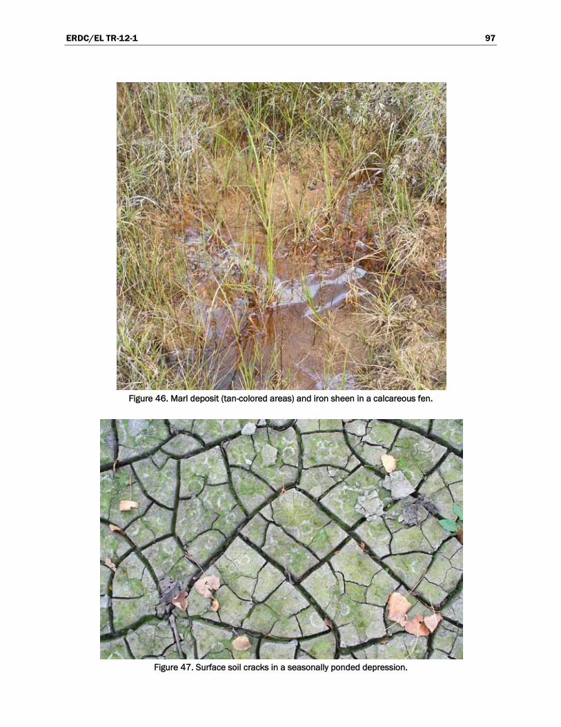
ERDC/EL TR-12-1 97
Figure 46. Marl deposit (tan-colored areas) and iron sheen in a calcareous fen.
Figure 47. Surface soil cracks in a seasonally ponded depression.
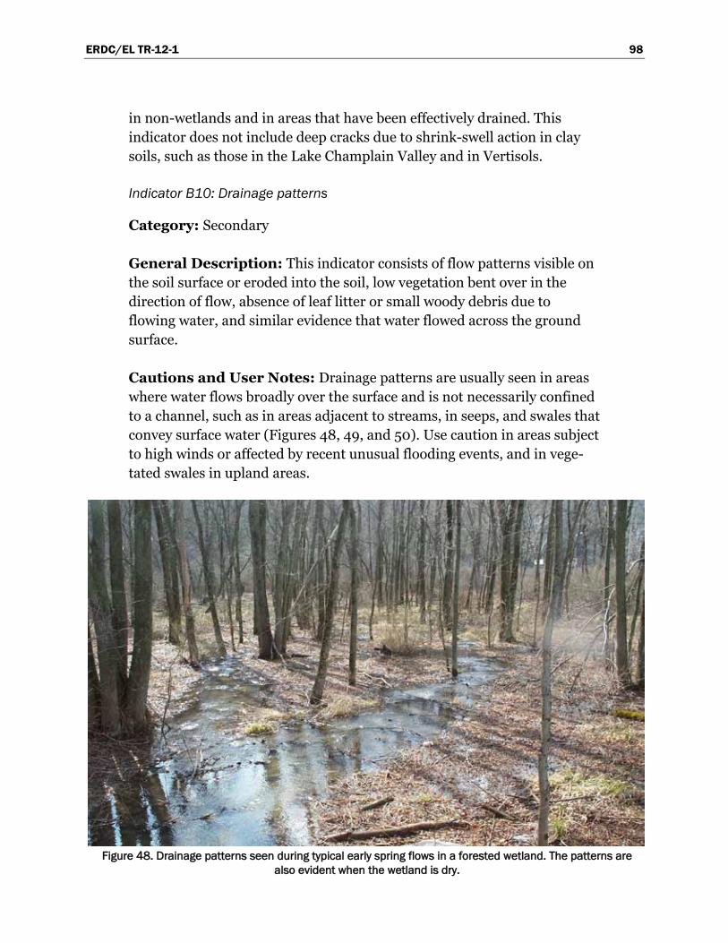
ERDC/EL TR-12-1 98
in non-wetlands and in areas that have been effectively drained. This indicator does not include deep cracks due to shrink-swell action in clay soils, such as those in the Lake Champlain Valley and in Vertisols.
Indicator B10: Drainage patterns
Category: Secondary
General Description: This indicator consists of flow patterns visible on the soil surface or eroded into the soil, low vegetation bent over in the direction of flow, absence of leaf litter or small woody debris due to flowing water, and similar evidence that water flowed across the ground surface.
Cautions and User Notes: Drainage patterns are usually seen in areas where water flows broadly over the surface and is not necessarily confined to a channel, such as in areas adjacent to streams, in seeps, and swales that convey surface water (Figures 48, 49, and 50). Use caution in areas subject to high winds or affected by recent unusual flooding events, and in vege-tated swales in upland areas.
Figure 48. Drainage patterns seen during typical early spring flows in a forested wetland. The patterns are
also evident when the wetland is dry.
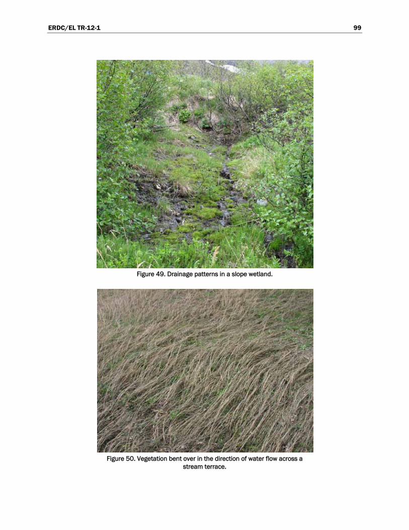
ERDC/EL TR-12-1 99
Figure 49. Drainage patterns in a slope wetland.
Figure 50. Vegetation bent over in the direction of water flow across a
stream terrace.
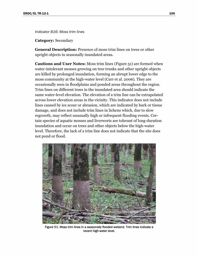
ERDC/EL TR-12-1 100
Indicator B16: Moss trim lines
Category: Secondary
General Description: Presence of moss trim lines on trees or other upright objects in seasonally inundated areas.
Cautions and User Notes: Moss trim lines (Figure 51) are formed when water-intolerant mosses growing on tree trunks and other upright objects are killed by prolonged inundation, forming an abrupt lower edge to the moss community at the high-water level (Carr et al. 2006). They are occasionally seen in floodplains and ponded areas throughout the region. Trim lines on different trees in the inundated area should indicate the same water-level elevation. The elevation of a trim line can be extrapolated across lower elevation areas in the vicinity. This indicator does not include lines caused by ice scour or abrasion, which are indicated by bark or tissue damage, and does not include trim lines in lichens which, due to slow regrowth, may reflect unusually high or infrequent flooding events. Cer-tain species of aquatic mosses and liverworts are tolerant of long-duration inundation and occur on trees and other objects below the high-water level. Therefore, the lack of a trim line does not indicate that the site does not pond or flood.
Figure 51. Moss trim lines in a seasonally flooded wetland. Trim lines indicate a
recent high-water level.
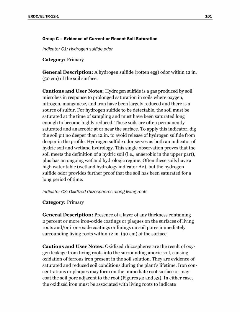
ERDC/EL TR-12-1 101
Group C – Evidence of Current or Recent Soil Saturation
Indicator C1: Hydrogen sulfide odor
Category: Primary
General Description: A hydrogen sulfide (rotten egg) odor within 12 in. (30 cm) of the soil surface.
Cautions and User Notes: Hydrogen sulfide is a gas produced by soil microbes in response to prolonged saturation in soils where oxygen, nitrogen, manganese, and iron have been largely reduced and there is a source of sulfur. For hydrogen sulfide to be detectable, the soil must be saturated at the time of sampling and must have been saturated long enough to become highly reduced. These soils are often permanently saturated and anaerobic at or near the surface. To apply this indicator, dig the soil pit no deeper than 12 in. to avoid release of hydrogen sulfide from deeper in the profile. Hydrogen sulfide odor serves as both an indicator of hydric soil and wetland hydrology. This single observation proves that the soil meets the definition of a hydric soil (i.e., anaerobic in the upper part), plus has an ongoing wetland hydrologic regime. Often these soils have a high water table (wetland hydrology indicator A2), but the hydrogen sulfide odor provides further proof that the soil has been saturated for a long period of time.
Indicator C3: Oxidized rhizospheres along living roots
Category: Primary
General Description: Presence of a layer of any thickness containing 2 percent or more iron-oxide coatings or plaques on the surfaces of living roots and/or iron-oxide coatings or linings on soil pores immediately surrounding living roots within 12 in. (30 cm) of the surface.
Cautions and User Notes: Oxidized rhizospheres are the result of oxy-gen leakage from living roots into the surrounding anoxic soil, causing oxidation of ferrous iron present in the soil solution. They are evidence of saturated and reduced soil conditions during the plant’s lifetime. Iron con-centrations or plaques may form on the immediate root surface or may coat the soil pore adjacent to the root (Figures 52 and 53). In either case, the oxidized iron must be associated with living roots to indicate
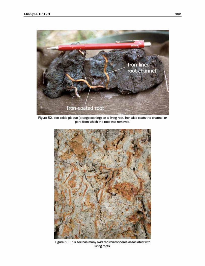
ERDC/EL TR-12-1 102
Figure 52. Iron-oxide plaque (orange coating) on a living root. Iron also coats the channel or
pore from which the root was removed.
Figure 53. This soil has many oxidized rhizospheres associated with
living roots.
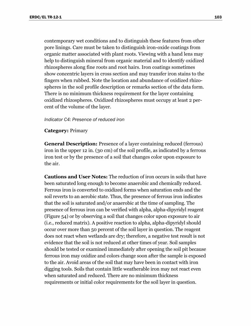
ERDC/EL TR-12-1 103
contemporary wet conditions and to distinguish these features from other pore linings. Care must be taken to distinguish iron-oxide coatings from organic matter associated with plant roots. Viewing with a hand lens may help to distinguish mineral from organic material and to identify oxidized rhizospheres along fine roots and root hairs. Iron coatings sometimes show concentric layers in cross section and may transfer iron stains to the fingers when rubbed. Note the location and abundance of oxidized rhizo-spheres in the soil profile description or remarks section of the data form. There is no minimum thickness requirement for the layer containing oxidized rhizospheres. Oxidized rhizospheres must occupy at least 2 per-cent of the volume of the layer.
Indicator C4: Presence of reduced iron
Category: Primary
General Description: Presence of a layer containing reduced (ferrous) iron in the upper 12 in. (30 cm) of the soil profile, as indicated by a ferrous iron test or by the presence of a soil that changes color upon exposure to the air.
Cautions and User Notes: The reduction of iron occurs in soils that have been saturated long enough to become anaerobic and chemically reduced. Ferrous iron is converted to oxidized forms when saturation ends and the soil reverts to an aerobic state. Thus, the presence of ferrous iron indicates that the soil is saturated and/or anaerobic at the time of sampling. The presence of ferrous iron can be verified with alpha, alpha-dipyridyl reagent (Figure 54) or by observing a soil that changes color upon exposure to air (i.e., reduced matrix). A positive reaction to alpha, alpha-dipyridyl should occur over more than 50 percent of the soil layer in question. The reagent does not react when wetlands are dry; therefore, a negative test result is not evidence that the soil is not reduced at other times of year. Soil samples should be tested or examined immediately after opening the soil pit because ferrous iron may oxidize and colors change soon after the sample is exposed to the air. Avoid areas of the soil that may have been in contact with iron digging tools. Soils that contain little weatherable iron may not react even when saturated and reduced. There are no minimum thickness requirements or initial color requirements for the soil layer in question.
ERDC/EL TR-12-1 104
Figure 54. When alpha, alpha-dipyridyl is applied to a soil containing reduced iron, a positive reaction is indicated by a pink or red coloration to the treated
area.
Indicator C6: Recent iron reduction in tilled soils
Category: Primary
General Description: Presence of a layer containing 2 percent or more redox concentrations as pore linings or soft masses in the tilled surface layer of soils cultivated within the last two years. The layer containing redox concentrations must be within the tilled zone or within 12 in. (30 cm) of the soil surface, whichever is shallower.
Cautions and User Notes: Cultivation breaks up or destroys redox features in the plow zone. The presence of redox features that are con-tinuous and unbroken indicates that the soil was saturated and reduced since the last episode of cultivation (Figure 55). Redox features often form around organic material, such as crop residue, incorporated into the tilled soil. Use caution with older features that may be broken up but not destroyed by tillage. Newly formed redox concentrations should have diffuse boundaries. The indicator is most reliable in areas that are culti-vated regularly, so that soil aggregates and older redox features are more likely to be broken up. If not obvious, information about the timing of last cultivation may be available from the land owner, other knowledgeable
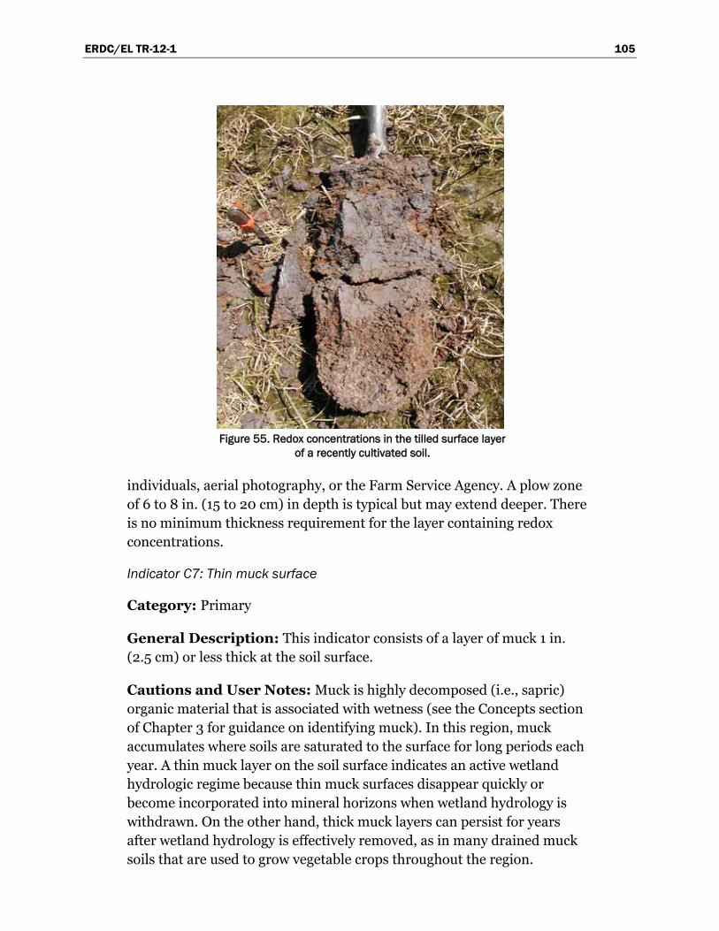
ERDC/EL TR-12-1 105
Figure 55. Redox concentrations in the tilled surface layer
of a recently cultivated soil.
individuals, aerial photography, or the Farm Service Agency. A plow zone of 6 to 8 in. (15 to 20 cm) in depth is typical but may extend deeper. There is no minimum thickness requirement for the layer containing redox concentrations.
Indicator C7: Thin muck surface
Category: Primary
General Description: This indicator consists of a layer of muck 1 in. (2.5 cm) or less thick at the soil surface.
Cautions and User Notes: Muck is highly decomposed (i.e., sapric) organic material that is associated with wetness (see the Concepts section of Chapter 3 for guidance on identifying muck). In this region, muck accumulates where soils are saturated to the surface for long periods each year. A thin muck layer on the soil surface indicates an active wetland hydrologic regime because thin muck surfaces disappear quickly or become incorporated into mineral horizons when wetland hydrology is withdrawn. On the other hand, thick muck layers can persist for years after wetland hydrology is effectively removed, as in many drained muck soils that are used to grow vegetable crops throughout the region.
ERDC/EL TR-12-1 106
Although thick muck layers also occur in wetlands, a muck layer greater than 1 in. thick does not qualify for this indicator. Use caution in areas with folistic surface layers (see the Concepts section of Chapter 3).
Indicator C2: Dry-season water table
Category: Secondary
General Description: Visual observation of the water table between 12 and 24 in. (30 and 60 cm) below the surface during the normal dry season or during a drier-than-normal year.
Cautions and User Notes: Due to normal seasonal fluctuations, water tables in wetlands often drop below 12 in. during the summer dry season. A water table between 12 and 24 in. during the dry season, or during an unusually dry year, likely indicates a normal wet-season water table within 12 in. of the surface. Sufficient time must be allowed for water to infiltrate into a newly dug hole and to stabilize at the water-table level. The required time will vary depending upon soil texture. In some cases, the water table can be determined by examining the wall of the soil pit and identifying the upper level at which water is seeping into the pit. For an accurate deter-mination of the water-table level, the soil pit, auger hole, or well should not penetrate any restrictive soil layer capable of perching water near the surface. Water tables in wetlands often drop well below 24 in. during dry periods. Therefore, a dry-season water table below 24 in. does not neces-sarily indicate a lack of wetland hydrology. See Chapter 5 (section on Wetlands that Periodically Lack Indicators of Wetland Hydrology) to determine average dry-season dates and drought periods. In the Remarks section of the data form or in a separate report, provide documentation for the conclusion that the site visit occurred during the normal dry season, recent rainfall has been below normal, or the area has been affected by drought. This indicator does not apply in agricultural areas that have controlled drainage structures for subsurface irrigation.
Indicator C8: Crayfish burrows
Category: Secondary
General Description: Presence of crayfish burrows, as indicated by openings in soft ground up to 2 in. (5 cm) in diameter, often surrounded by chimney-like mounds of excavated mud.
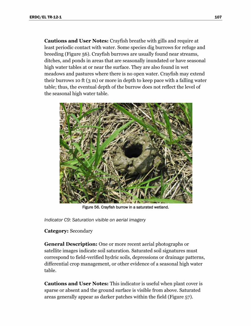
ERDC/EL TR-12-1 107
Cautions and User Notes: Crayfish breathe with gills and require at least periodic contact with water. Some species dig burrows for refuge and breeding (Figure 56). Crayfish burrows are usually found near streams, ditches, and ponds in areas that are seasonally inundated or have seasonal high water tables at or near the surface. They are also found in wet meadows and pastures where there is no open water. Crayfish may extend their burrows 10 ft (3 m) or more in depth to keep pace with a falling water table; thus, the eventual depth of the burrow does not reflect the level of the seasonal high water table.
Figure 56. Crayfish burrow in a saturated wetland.
Indicator C9: Saturation visible on aerial imagery
Category: Secondary
General Description: One or more recent aerial photographs or satellite images indicate soil saturation. Saturated soil signatures must correspond to field-verified hydric soils, depressions or drainage patterns, differential crop management, or other evidence of a seasonal high water table.
Cautions and User Notes: This indicator is useful when plant cover is sparse or absent and the ground surface is visible from above. Saturated areas generally appear as darker patches within the field (Figure 57).
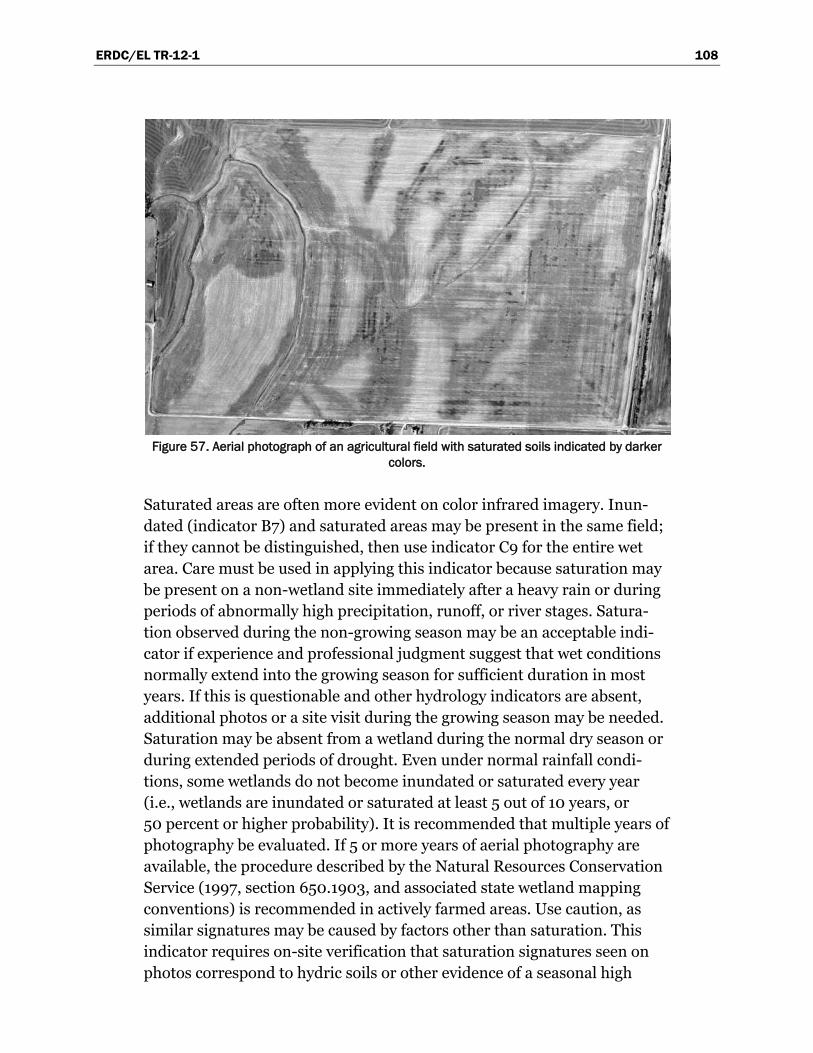
ERDC/EL TR-12-1 108
Figure 57. Aerial photograph of an agricultural field with saturated soils indicated by darker
colors.
Saturated areas are often more evident on color infrared imagery. Inun-dated (indicator B7) and saturated areas may be present in the same field; if they cannot be distinguished, then use indicator C9 for the entire wet area. Care must be used in applying this indicator because saturation may be present on a non-wetland site immediately after a heavy rain or during periods of abnormally high precipitation, runoff, or river stages. Satura-tion observed during the non-growing season may be an acceptable indi-cator if experience and professional judgment suggest that wet conditions normally extend into the growing season for sufficient duration in most years. If this is questionable and other hydrology indicators are absent, additional photos or a site visit during the growing season may be needed. Saturation may be absent from a wetland during the normal dry season or during extended periods of drought. Even under normal rainfall condi-tions, some wetlands do not become inundated or saturated every year (i.e., wetlands are inundated or saturated at least 5 out of 10 years, or 50 percent or higher probability). It is recommended that multiple years of photography be evaluated. If 5 or more years of aerial photography are available, the procedure described by the Natural Resources Conservation Service (1997, section 650.1903, and associated state wetland mapping conventions) is recommended in actively farmed areas. Use caution, as similar signatures may be caused by factors other than saturation. This indicator requires on-site verification that saturation signatures seen on photos correspond to hydric soils or other evidence of a seasonal high
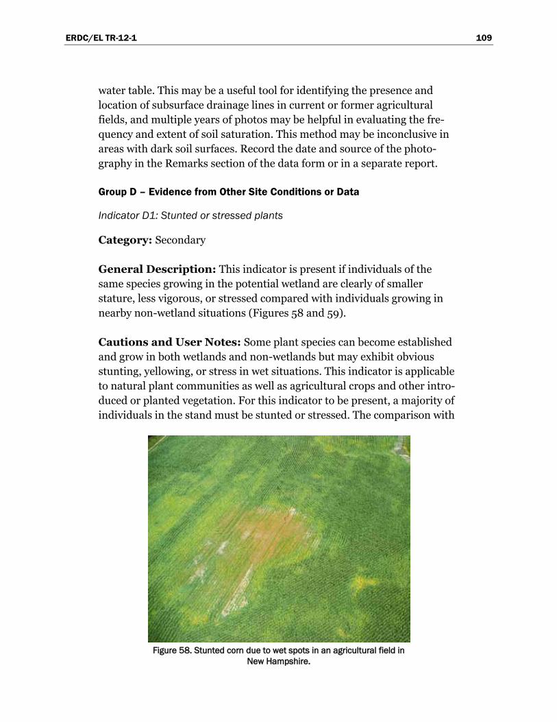
ERDC/EL TR-12-1 109
water table. This may be a useful tool for identifying the presence and location of subsurface drainage lines in current or former agricultural fields, and multiple years of photos may be helpful in evaluating the fre-quency and extent of soil saturation. This method may be inconclusive in areas with dark soil surfaces. Record the date and source of the photo-graphy in the Remarks section of the data form or in a separate report.
Group D – Evidence from Other Site Conditions or Data
Indicator D1: Stunted or stressed plants
Category: Secondary
General Description: This indicator is present if individuals of the same species growing in the potential wetland are clearly of smaller stature, less vigorous, or stressed compared with individuals growing in nearby non-wetland situations (Figures 58 and 59).
Cautions and User Notes: Some plant species can become established and grow in both wetlands and non-wetlands but may exhibit obvious stunting, yellowing, or stress in wet situations. This indicator is applicable to natural plant communities as well as agricultural crops and other intro-duced or planted vegetation. For this indicator to be present, a majority of individuals in the stand must be stunted or stressed. The comparison with
Figure 58. Stunted corn due to wet spots in an agricultural field in
New Hampshire.
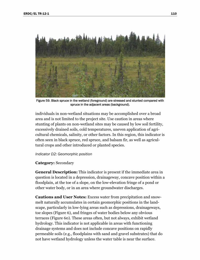
ERDC/EL TR-12-1 110
Figure 59. Black spruce in the wetland (foreground) are stressed and stunted compared with
spruce in the adjacent areas (background).
individuals in non-wetland situations may be accomplished over a broad area and is not limited to the project site. Use caution in areas where stunting of plants on non-wetland sites may be caused by low soil fertility, excessively drained soils, cold temperatures, uneven application of agri-cultural chemicals, salinity, or other factors. In this region, this indicator is often seen in black spruce, red spruce, and balsam fir, as well as agricul-tural crops and other introduced or planted species.
Indicator D2: Geomorphic position
Category: Secondary
General Description: This indicator is present if the immediate area in question is located in a depression, drainageway, concave position within a floodplain, at the toe of a slope, on the low-elevation fringe of a pond or other water body, or in an area where groundwater discharges.
Cautions and User Notes: Excess water from precipitation and snow-melt naturally accumulates in certain geomorphic positions in the land-scape, particularly in low-lying areas such as depressions, drainageways, toe slopes (Figure 6), and fringes of water bodies below any obvious terraces (Figure 60). These areas often, but not always, exhibit wetland hydrology. This indicator is not applicable in areas with functioning drainage systems and does not include concave positions on rapidly permeable soils (e.g., floodplains with sand and gravel substrates) that do not have wetland hydrology unless the water table is near the surface.
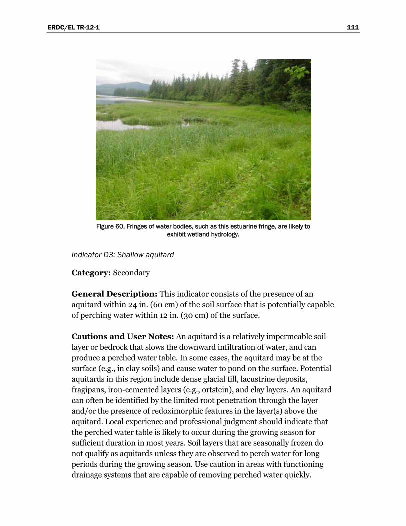
ERDC/EL TR-12-1 111
Figure 60. Fringes of water bodies, such as this estuarine fringe, are likely to
exhibit wetland hydrology.
Indicator D3: Shallow aquitard
Category: Secondary
General Description: This indicator consists of the presence of an aquitard within 24 in. (60 cm) of the soil surface that is potentially capable of perching water within 12 in. (30 cm) of the surface.
Cautions and User Notes: An aquitard is a relatively impermeable soil layer or bedrock that slows the downward infiltration of water, and can produce a perched water table. In some cases, the aquitard may be at the surface (e.g., in clay soils) and cause water to pond on the surface. Potential aquitards in this region include dense glacial till, lacustrine deposits, fragipans, iron-cemented layers (e.g., ortstein), and clay layers. An aquitard can often be identified by the limited root penetration through the layer and/or the presence of redoximorphic features in the layer(s) above the aquitard. Local experience and professional judgment should indicate that the perched water table is likely to occur during the growing season for sufficient duration in most years. Soil layers that are seasonally frozen do not qualify as aquitards unless they are observed to perch water for long periods during the growing season. Use caution in areas with functioning drainage systems that are capable of removing perched water quickly.
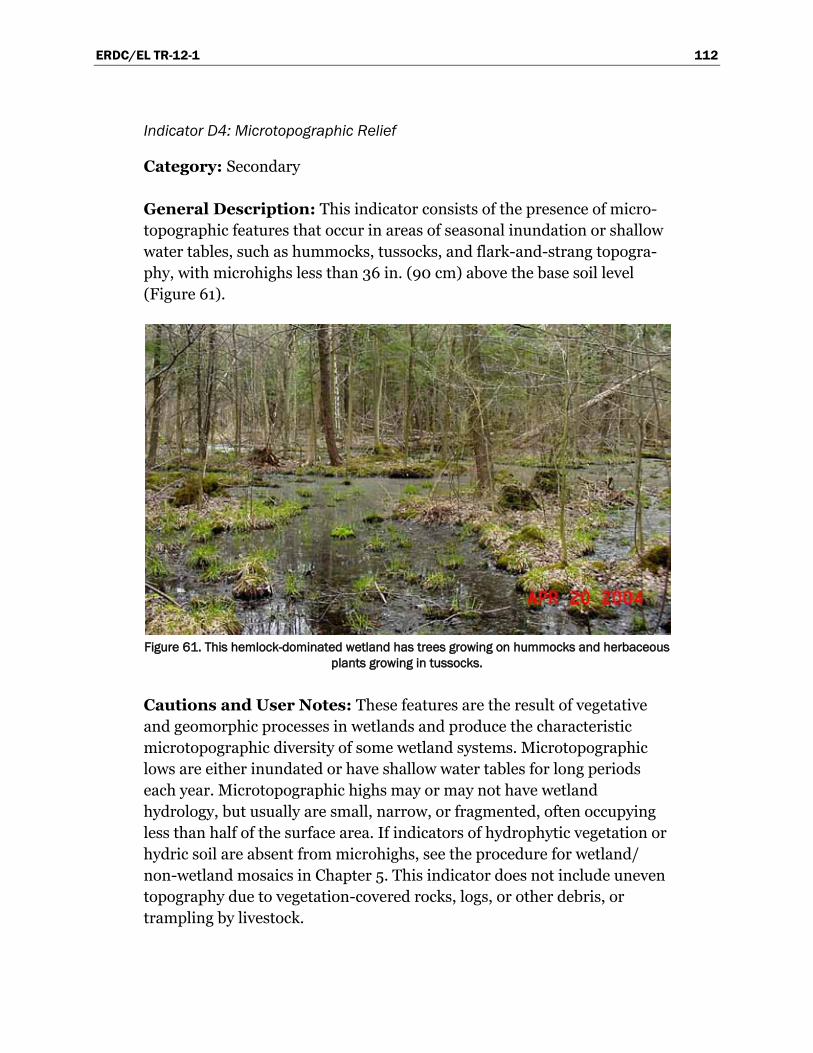
ERDC/EL TR-12-1 112
Indicator D4: Microtopographic Relief
Category: Secondary
General Description: This indicator consists of the presence of micro-topographic features that occur in areas of seasonal inundation or shallow water tables, such as hummocks, tussocks, and flark-and-strang topogra-phy, with microhighs less than 36 in. (90 cm) above the base soil level (Figure 61).
Figure 61. This hemlock-dominated wetland has trees growing on hummocks and herbaceous
plants growing in tussocks.
Cautions and User Notes: These features are the result of vegetative and geomorphic processes in wetlands and produce the characteristic microtopographic diversity of some wetland systems. Microtopographic lows are either inundated or have shallow water tables for long periods each year. Microtopographic highs may or may not have wetland hydrology, but usually are small, narrow, or fragmented, often occupying less than half of the surface area. If indicators of hydrophytic vegetation or hydric soil are absent from microhighs, see the procedure for wetland/ non-wetland mosaics in Chapter 5. This indicator does not include uneven topography due to vegetation-covered rocks, logs, or other debris, or trampling by livestock.
ERDC/EL TR-12-1 113
Indicator D5: FAC-neutral test
Category: Secondary
General Description: The plant community passes the FAC-neutral test.
Cautions and User Notes: The FAC-neutral test is performed by compiling a list of dominant plant species across all strata in the community, and dropping from the list any species with a Facultative indicator status (i.e., FAC). The FAC-neutral test is met if more than 50 percent of the remaining dominant species are rated FACW and/or OBL. This indicator can be used in communities that contain no FAC dominants. If there are an equal number of dominants that are OBL and FACW versus FACU and UPL, or if all dominants are FAC, non-dominant species should be considered.
ERDC/EL TR-12-1 114
5 Difficult Wetland Situations in the Northcentral and Northeast Region
Introduction
Some wetlands can be difficult to identify because wetland indicators may be missing due to natural processes or recent disturbances. This chapter provides guidance for making wetland determinations in difficult-to-identify wetland situations in the Northcentral and Northeast Region. It includes regional examples of problem area wetlands and atypical situ-ations as defined in the Corps Manual, as well as other situations that can make wetland delineation more challenging. Problem area wetlands are naturally occurring wetland types that lack indicators of hydrophytic vegetation, hydric soil, or wetland hydrology periodically due to normal seasonal or annual variability, or permanently due to the nature of the soils or plant species on the site. Atypical situations are wetlands in which vegetation, soil, and/or hydrology indicators are absent due to recent human activities or natural events. In addition, this chapter addresses certain procedural problems (e.g., wetland/non-wetland mosaics) that can make wetland determinations in the region difficult or confusing. The chapter is organized into the following sections:
• Lands Used for Agriculture and Silviculture • Problematic Hydrophytic Vegetation • Problematic Hydric Soils • Wetlands that Periodically Lack Indicators of Wetland Hydrology • Wetland/Non-Wetland Mosaics
The list of difficult wetland situations presented in this chapter is not intended to be exhaustive and other problematic situations may exist in the region. See the Corps Manual for general guidance. Furthermore, more than one wetland factor (i.e., vegetation, soil, and/or hydrology) may be disturbed or problematic on a given site. In general, wetland determina-tions on difficult or problematic sites must be based on the best infor-mation available to the field inspector, interpreted in light of his or her professional experience and knowledge of the ecology of wetlands in the region.
ERDC/EL TR-12-1 115
Lands used for agriculture and silviculture
Agriculture and silviculture are important land uses in the Northcentral and Northeast Region, and both of these activities present challenges to wetland identification and delineation. Wetlands used for agriculture or silviculture often lack a natural plant community and may be planted to crops, pasture species, or desirable tree species and may be altered by mowing, grazing, herbicide use, or other management practices. Soils may be disturbed by cultivation, land clearing, grading, or bedding, at least in the surface layers, and hydrology may or may not be manipulated. Some areas that are used for agriculture or silviculture still retain wetland hydrology. In other areas, historic wetlands have been effectively drained and no longer meet wetland hydrology standards. Relict wetland indi-cators may still be present in these areas, making it difficult to distinguish current wetlands from those that have been effectively drained. In addi-tion, agricultural activities can include improved groundwater manage-ment, involving the manipulation of water tables to conserve both water and nutrients (e.g., Frankenberger et al. 2006).
Agricultural and silvicultural drainage systems use ditches, subsurface drainage lines or “tiles,” and water-control structures to manipulate the water table and improve conditions for crops or other desired species. A freely flowing ditch or drainage line depresses the water table within a certain lateral distance or zone of influence (Figure 62). The effectiveness of drainage in an area depends in part on soil characteristics, the timing and amount of rainfall, and the depth and spacing of ditches or drains. Wetland determinations on current and former agricultural or silvicultural lands must consider whether a drainage system is present, how it is designed to function, and whether it is effective in removing wetland hydrology from the area.
A number of information sources and tools are listed below to help deter-mine whether wetlands are present on lands where vegetation, soils, hydrology, or a combination of these factors have been manipulated. Some of these options are discussed in more detail later in this chapter under the appropriate section headings.
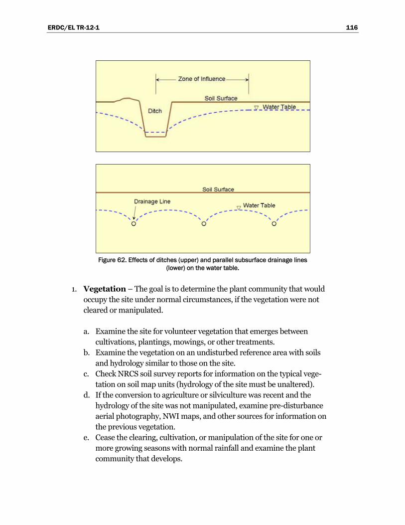
ERDC/EL TR-12-1 116
Figure 62. Effects of ditches (upper) and parallel subsurface drainage lines
(lower) on the water table.
1. Vegetation – The goal is to determine the plant community that would occupy the site under normal circumstances, if the vegetation were not cleared or manipulated. a. Examine the site for volunteer vegetation that emerges between
cultivations, plantings, mowings, or other treatments. b. Examine the vegetation on an undisturbed reference area with soils
and hydrology similar to those on the site. c. Check NRCS soil survey reports for information on the typical vege-
tation on soil map units (hydrology of the site must be unaltered). d. If the conversion to agriculture or silviculture was recent and the
hydrology of the site was not manipulated, examine pre-disturbance aerial photography, NWI maps, and other sources for information on the previous vegetation.
e. Cease the clearing, cultivation, or manipulation of the site for one or more growing seasons with normal rainfall and examine the plant community that develops.
ERDC/EL TR-12-1 117
2. Soils – Tilling of agricultural land mixes the surface layer(s) of the soil and may cause compaction below the tilled zone (i.e., a “plow pan”) due to the weight and repeated passage of farm machinery. Similar disturbance to surface soils may also occur in areas managed for silviculture. Neverthe-less, a standard soil profile description and examination for hydric soil indicators are often sufficient to determine whether hydric soils are present. Other options and information sources include the following: a. Examine NRCS soil survey maps and the local hydric soils list for the
likely presence of hydric soils on the site. b. Examine the soils on an undisturbed reference area with landscape
position, parent materials, and hydrology similar to those on the site. c. Use alpha, alpha-dipyridyl reagent to check for the presence of reduced
iron during the normal wet portion of the growing season, or note whether the soil changes color upon exposure to the air.
d. Monitor the site in relation to the appropriate wetland hydrology or hydric soils technical standard.
3. Hydrology – The goal is to determine whether wetland hydrology is present on a managed site under normal circumstances, as defined in the Corps Manual and subsequent guidance. These sites may or may not have been hydrologically manipulated. a. Examine the site for existing indicators of wetland hydrology. If the
natural hydrology of the site has been permanently altered, discount any indicators known to have been produced before the alteration (e.g., relict water marks or drift lines).
b. In agricultural areas (e.g., row crops, hayfields, tree farms, nurseries, orchards, and others) examine five or more years of aerial photographs for wetness signatures listed in Part 513.30 of the National Food Security Act Manual (USDA Natural Resources Conservation Service 1994) or in wetland mapping conventions available from NRCS offices or online in the electronic Field Office Technical Guide (eFOTG) (http://www.nrcs.usda.gov/technical/efotg/). Use the procedure given by the USDA Natural Resources Conservation Service (1997) to determine whether wetland hydrology is present.
c. Estimate the effects of ditches and subsurface drainage systems using scope-and-effect equations (USDA Natural Resources Conservation Service 1997). A web application to analyze data using various models is available at http://www.wli.nrcs.usda.gov/technical/web_tool/tools_java.html.
ERDC/EL TR-12-1 118
Scope-and-effect equations are approximations only and may not reflect actual field conditions. Their results should be verified by comparison with other techniques for evaluating drainage and should not overrule onsite evidence of wetland hydrology.
d. Use state drainage guides to estimate the effectiveness of an existing drainage system (USDA Natural Resources Conservation Service 1997). Drainage guides may be available from NRCS offices. Cautions noted in item c above also apply to the use of drainage guides. In addition, Corps of Engineers district offices should be consulted for locally developed techniques to evaluate wetland drainage.
e. Use hydrologic models (e.g., runoff, surface water, and groundwater models) to determine whether wetland hydrology is present (e.g., USDA Natural Resources Conservation Service 1997).
f. Monitor the hydrology of the site in relation to the appropriate wetland hydrology technical standard (U. S. Army Corps of Engineers 2005).
Problematic hydrophytic vegetation
Description of the problem
Many factors affect the structure and composition of plant communities in the region, including climatic variability, spread of exotic species, agri-cultural and silvicultural use, and other human land-use practices. As a result, some wetlands may exhibit indicators of hydric soil and wetland hydrology but lack any of the hydrophytic vegetation indicators presented in Chapter 2, at least at certain times. To identify and delineate these wetlands may require special sampling procedures or additional analysis of factors affecting the site. To the extent possible, the hydrophytic vegeta-tion decision should be based on the plant community that is normally present during the wet portion of the growing season in a normal rainfall year. The following procedure addresses several examples of problematic vegetation situations in the Northcentral and Northeast Region.
Procedure
Problematic hydrophytic vegetation can be identified using a combination of observations made in the field and/or supplemental information from the scientific literature and other sources. These procedures should be applied only where indicators of hydric soil and wetland hydrology are present, unless one or both of these factors is also disturbed or
ERDC/EL TR-12-1 119
problematic, but no indicators of hydrophytic vegetation are evident. The following procedures are recommended:
1. Verify that at least one indicator of hydric soil and one primary or two secondary indicators of wetland hydrology are present. If indicators of either hydric soil or wetland hydrology are absent, the area is likely non-wetland unless soil and/or hydrology are also disturbed or problematic. If indicators of hydric soil and wetland hydrology are present (or are absent due to disturbance or other problem situations), proceed to step 2.
2. Verify that the area is in a landscape position that is likely to collect or
concentrate water. If the landscape setting is appropriate, proceed to step 3. Appropriate settings include the following. a. Concave surface (e.g., depression or swale) b. Active floodplain or low terrace c. Level or nearly level area (e.g., 0- to 3-percent slope) d. Toe slope (Figure 6) or an area of convergent slopes (Figure 5) e. Fringe of another wetland or water body f. Area with a restrictive soil layer or aquitard within 24 in. (60 cm) of the
surface g. Area where groundwater discharges (e.g., a seep) h. Other (explain in field notes why this area is likely to be inundated or
saturated for long periods)
3. Use one or more of the approaches described in step 4 (Specific Problematic Vegetation Situations below) or step 5 (General Approaches to Problematic Hydrophytic Vegetation on page 131) to determine whether the vegetation is hydrophytic. In the remarks section of the data form or in the delineation report, explain the rationale for concluding that the plant community is hydrophytic even though indicators of hydrophytic vege-tation described in Chapter 2 were not observed.
4. Specific Problematic Vegetation Situations a. Temporal shifts in vegetation. As described in Chapter 2, the species
composition of some wetland plant communities in the region can change in response to seasonal weather patterns and long-term climatic fluctuations. Wetland types that are influenced by these shifts include Great Lakes coastal wetlands, vernal pools, interdunal swales,
ERDC/EL TR-12-1 120
wet meadows, wet prairies, seeps, and springs. Lack of hydrophytic vegetation during the dry season, when FACU and UPL warm-season grasses and annuals dominate many areas, should not immediately eliminate a site from consideration as a wetland, because the site may have been dominated by wetland species earlier in the growing season. A site qualifies for further consideration if the plant community at the time of sampling does not exhibit hydrophytic vegetation indicators, but indicators of hydric soil and wetland hydrology are present or known to be disturbed or problematic. The following sampling and analytical approaches are recommended in these situations: (1) Seasonal Shifts in Plant Communities
(a) If possible, return to the site during the normal wet portion of
the growing season (generally in early spring) and re-examine the site for indicators of hydrophytic vegetation.
(b) Examine the site for identifiable plant remains, either alive or dead, or other evidence that the plant community that was present during the normal wet portion of the growing season was hydrophytic.
(c) Use off-site data sources to determine whether the plant community that is normally present during the wet portion of the growing season is hydrophytic. Appropriate data sources include early growing season aerial photography, NWI maps, soil survey reports, remotely sensed data, public interviews, state wetland conservation plans, and previous reports about the site. If necessary, re-examine the site early in the growing season to verify the hydrophytic vegetation determination.
(d) If the vegetation on the site is substantially the same as that on a wetland reference site having similar soils, landscape position, and known wetland hydrology, then consider the vegetation to be hydrophytic (see step 5c in this procedure for more information).
(e) If the hydrophytic status of the vegetation during the normal wet portion of the growing season in a normal rainfall year cannot be determined, make the wetland determination based on indicators of hydric soil and wetland hydrology.
ERDC/EL TR-12-1 121
(2) Prolonged Dry to Drought Conditions (lasting more than one growing season) (a) Investigate climate records (e.g., WETS tables, drought indices)
to determine if the area is under the influence of a drought or prolonged dry conditions (for more information, see the section on Wetlands that Periodically Lack Indicators of Wetland Hydrology later in this chapter). If so, evaluate any off-site data that provide information on the plant community that exists on the site during normal years, including aerial photography, Farm Service Agency annual crop slides, NWI maps, other remote sensing data, soil survey reports, public interviews, NRCS hydrology tools (USDA Natural Resources Conservation Service 1997), and previous site reports. Determine whether the vegetation that is present during normal years is hydrophytic.
(b) If the vegetation on the affected site is substantially the same as that on a wetland reference site in the same general area having similar soils and known wetland hydrology, then consider the vegetation to be hydrophytic (see step 5c in this procedure).
(c) If the hydrophytic status of the vegetation during the normal wet portion of the growing season in a normal rainfall year cannot be determined, make the wetland determination based on indicators of hydric soil and wetland hydrology.
(3) Long-Term Fluctuations in Lake Levels. Water levels in lakes and ponds rise and fall depending upon annual precipitation patterns. These changes may induce short- or long-term shifts in fringing vegetation depending upon the duration of the wet or dry con-ditions. The Great Lakes have experienced significant periodic fluctuations in water levels since the early part of the twentieth century. During years with high lake levels, large areas of coastal vegetation may be inundated and converted to open water. During periods with low lake levels, some fringe wetlands may dry out and their vegetation may shift to non-hydrophytic plant communities. Similar vegetation changes may be observed on a smaller scale around the margins of other lakes and ponds across the North-central and Northeast Region (Tiner 2005). To determine the plant community that is present during normal lake levels, the following approaches are recommended.
ERDC/EL TR-12-1 122
(a) Determine whether water levels have been higher or lower than the long-term average by examining current and historical water-level data, such as those available for the Great Lakes from the Corps of Engineers Detroit District (http://www.lre.usace.army.mil/greatlakes/hh/greatlakeswaterlevels/). If water levels have been appreciably higher or lower than average for two or more consecutive years, examine off-site data sources to determine whether the plant community that is present on the site during years with normal lake levels is hydrophytic. Appropriate data sources include early growing-season aerial photography taken during normal years, NWI maps, soil survey reports, other remotely sensed data, interviews with the land owner and other knowledgeable people, state wetland conser-vation plans, and previous reports about the site.
(b) Examine the existing vegetation on the site, emphasizing long-lived woody and other perennial plant species. Discount annual and other short-lived species that may have become established during the period of unusually high or low lake levels.
(c) If the vegetation on the site is substantially the same as that on a wetland reference site on the same lake having similar soils, landscape position, and known wetland hydrology, then con-sider the vegetation to be hydrophytic (see step 5c in this procedure for more information).
(d) If the hydrophytic status of the vegetation during years with normal lake levels cannot be determined, make the wetland determination based on indicators of hydric soil and wetland hydrology.
b. Vernal pools. Vernal pools are small, seasonal water bodies that pond water from the time of snowmelt into early to mid-summer. They are common throughout the glaciated Northcentral and Northeast Region, although most remaining pools are located in forested settings. The pools may be situated within wetlands or non-wetlands. They are characterized by vernal-pool-specific fauna, particularly amphibians and invertebrates that require the pools to complete their life cycles (Colburn 2004). The vegetation in and around these pools is influ-enced by the seasonal hydrology. During the early part of the growing season, they may lack herbaceous vegetation due to inundation and it may be necessary to base the hydrophytic vegetation decision solely on woody plants. Where woody vegetation is lacking, herbaceous
ERDC/EL TR-12-1 123
vegetation should be examined later in the growing season. In pools that retain water for very long periods, vegetation may not become well established even during drier periods. During the driest times of the year, or in drought years, some pools become dominated by upland plants, particularly annuals. The following approaches are recom-mended for evaluating vernal pools where indicators of hydric soil and wetland hydrology are present, but hydrophytic vegetation is not evident at the time of the site visit. (1) If the pool is filled with water at the time of the visit, emergent
vegetation is absent, and a follow-up site visit is practical, then return to the site soon after seasonal draw-down and check for indicators of hydrophytic vegetation.
(2) If the site is visited during the dry season, vegetation in the potential pool area is dominated by upland species (particularly annuals), and a follow-up site visit is practical, then revisit the site during the normal wet portion of the growing season and check again for indicators of hydrophytic vegetation.
(3) If the hydrophytic status of the vegetation during the normal wet portion of the growing season in a normal rainfall year cannot be determined, make the wetland determination based on indicators of hydric soil and wetland hydrology.
c. Areas affected by grazing. Both short- and long-term grazing can cause shifts in dominant species in the vegetation. For instance, trampling by large herbivores can cause soil compaction, altering soil permeability and infiltration rates, and affecting the plant community. Grazers can also influence the abundance of plant species by selectively grazing certain palatable species or avoiding less palatable species. This shift in species composition due to grazing can influence the hydro-phytic vegetation determination. Be aware that shifts in both direc-tions, favoring either wetland species or upland species, can occur in these situations. Limited grazing does not necessarily affect the out-come of a hydrophytic vegetation decision. However, the following approaches are recommended in cases where the effects of grazing are so great that the hydrophytic vegetation determination would be unreliable or misleading.
ERDC/EL TR-12-1 124
(1) Examine the vegetation on a nearby, ungrazed reference site having similar soils and hydrologic conditions. Ungrazed areas may be present on adjacent properties or in fenced exclosures or stream-side management zones. Assume that the same plant community would exist on the grazed site, in the absence of grazing.
(2) If feasible, remove livestock or fence representative livestock exclu-sion areas to allow the vegetation time to recover from grazing, and reevaluate the vegetation during the next growing season.
(3) If grazing was initiated recently, use offsite data sources such as aerial photography, NWI maps, and interviews with the land owner and other persons familiar with the site or area to determine what plant community was present on the site before grazing began. If the previously ungrazed community was hydrophytic, then con-sider the current vegetation to be hydrophytic.
(4) If an appropriate ungrazed area cannot be located or if the ungrazed vegetation condition cannot be determined, make the wetland determination based on indicators of hydric soils and wetland hydrology.
d. Managed plant communities. Natural plant communities throughout the region have been replaced with agricultural crops or are otherwise managed to meet human goals. Examples include clearing of woody species on grazed pasture land; periodic disking, plowing, or mowing; planting of native and non-native species (including cultivars or planted species that have escaped and become established on other sites); use of herbicides; silvicultural activities; and suppression of wildfires. These actions can result in elimination of certain species and their replacement with other species, changes in abundance of certain plants, and shifts in dominant species, possibly influencing a hydro-phytic vegetation determination. The following approaches are recom-mended if the natural vegetation has been altered through manage-ment to such an extent that a hydrophytic vegetation determination is not possible or would be unreliable: (1) Examine the vegetation on a nearby, unmanaged reference site
having similar soils and hydrologic conditions. Assume that the same plant community would exist on the managed site in the
ERDC/EL TR-12-1 125
absence of human alteration.
(2) For recently cleared or tilled areas (not planted or seeded), leave representative areas unmanaged for at least one growing season with normal rainfall and reevaluate the vegetation.
(3) If management was initiated recently, use offsite data sources such as aerial photography, NWI maps, and interviews with the land owner and other persons familiar with the area to determine what plant community was present on the site before the management occurred.
(4) If the unmanaged vegetation condition cannot be determined, make the wetland determination based on indicators of hydric soil and wetland hydrology.
e. Areas affected by fires, floods, and other natural disturbances. Fires, floods, and other natural disturbances can dramatically alter the vege-tation on a site. Vegetation can be completely or partially removed, or its composition altered, depending upon the intensity of the distur-bance. Limited disturbance does not necessarily affect the investi-gator’s ability to determine whether the plant community is or is not hydrophytic. However, if the vegetation on a site has been removed or made unidentifiable by a recent fire, flood, or other disturbance, then one or more of the following approaches may be used to determine whether the vegetation present before the disturbance was hydro-phytic. Additional guidance can be found in Part IV, Section F (Atypical Situations) of the Corps Manual. (1) Examine the vegetation on a nearby, undisturbed reference site
having similar soils and hydrologic conditions. Assume that the same plant community would exist on the disturbed site in the absence of disturbance.
(2) Use offsite data sources such as aerial photography, NWI maps, and interviews with knowledgeable people to determine what plant community was present on the site before the disturbance.
(3) If the undisturbed vegetation condition cannot be determined, make the wetland determination based on indicators of hydric soil and wetland hydrology.
ERDC/EL TR-12-1 126
f. Areas dominated exclusively by non-vascular plants. In areas that lack vascular plants but are dominated by peat mosses (e.g., Sphag-num spp.), the vegetation should be considered to be hydrophytic if indicators of hydric soil and wetland hydrology are present, the land-scape position is appropriate for wetlands, and hydrology has not been altered.
5. General Approaches to Problematic Hydrophytic Vegetation. The follow-ing general procedures are provided to identify hydrophytic vegetation in difficult situations not necessarily associated with specific vegetation types or management practices, including wetlands dominated by FACU, NI, NO, or unlisted species that are functioning as hydrophytes. The following recommended approaches should be applied only where indicators of hydric soil and wetland hydrology are present (or are absent due to disturbance or other problem situations) and the landscape position is appropriate to collect or concentrate water, but indicators of hydrophytic vegetation are not evident. a. FACU species that commonly dominate wetlands. The following
FACU species occur in and dominate many wetlands in the North-central and Northeast Region and may cause a wetland plant com-munity to fail to meet any of the hydrophytic vegetation indicators described in Chapter 2: eastern hemlock (Tsuga canadensis), eastern white pine (Pinus strobus), red spruce (Picea rubens), pitch pine (Pinus rigida), Virginia creeper (Parthenocissus quinquefolia), springbeauty (Claytonia virginica), and the following non-native species: common buckthorn (Rhamnus cathartica), multiflora rose (Rosa multiflora), tartarian honeysuckle (Lonicera tatarica), and Morrow’s honeysuckle (L. morrowii) (indicator statuses may vary by plant list region). If the potential wetland area lacks hydrophytic vegetation indicators due to the presence of one or more of the FACU species listed above, use the following procedure to make the hydrophytic vegetation determination: (1) At each sampling point in the potential wetland, drop any FACU
species listed above from the vegetation data, and compile the species list and coverage data for the remaining species in the community.
ERDC/EL TR-12-1 127
(2) Reevaluate the remaining vegetation using hydrophytic vegetation indicators 2 (Dominance Test) and/or 3 (Prevalence Index). If either indicator is met, then the vegetation is hydrophytic.
b. Direct hydrologic observations. Verify that the plant community occurs in an area subject to prolonged inundation or soil saturation during the growing season. This can be done by visiting the site at 2- to 3-day intervals during the portion of the growing season when surface water is most likely to be present or water tables are normally high. Hydrophytic vegetation is considered to be present, and the site is a wetland, if surface water is present and/or the water table is 12 in. (30 cm) or less from the surface for 14 or more consecutive days during the growing season during a period when antecedent precipitation has been normal or drier than normal. If necessary, microtopographic highs and lows should be evaluated separately. The normality of the current year’s rainfall must be considered in interpreting field results, as well as the likelihood that wet conditions will occur on the site at least every other year (for more information, see the section on “Wetlands that Periodically Lack Indicators of Wetland Hydrology” in this chapter).
c. Reference sites with known hydrology. If indicators of hydric soil and wetland hydrology are present, the site may be considered to be a wetland if the landscape setting, topography, soils, and vegetation are substantially the same as those on nearby wetland reference areas whose hydrology is known. Hydrologic characteristics of wetland reference areas should be documented through long-term monitoring or by application of the procedure described in item 5b above. Reference sites should be minimally disturbed and provide long-term access. Soils, vegetation, and hydrologic conditions should be thoroughly documented and the data kept on file in the district or field office.
d. Technical literature. Published and unpublished scientific literature may be used to support a decision to treat specific FACU species or species with no assigned indicator status (e.g., NI, NO, or unlisted) as hydrophytes or certain plant communities as hydrophytic. Preferably, this literature should discuss the species’ natural distribution along the moisture gradient, its capabilities and adaptations for life in wetlands, wetland types in which it is typically found, or other wetland species with which it is commonly associated.
ERDC/EL TR-12-1 128
Problematic hydric soils
Description of the problem
Soils with faint or no indicators
Some soils that meet the hydric soil definition may not exhibit any of the indicators presented in Chapter 3. These problematic hydric soils exist for a number of reasons and their proper identification requires additional information, such as landscape position, presence or absence of restrictive soil layers, or information about hydrology. This section describes several soil situations in the Northcentral and Northeast Region that are con-sidered to be hydric if additional requirements are met. In some cases, these hydric soils may appear to be non-hydric due to the color of the parent material from which the soils developed. In others, the lack of hydric soil indicators is due to conditions (e.g., red parent materials) that inhibit the development of redoximorphic features despite prolonged soil saturation and anoxia. In addition, recently developed wetlands may lack hydric soil indicators because insufficient time has passed for their development. Examples of problematic hydric soils in the region include, but are not limited to, the following.
1. Sandy Soils. The development of hydric soil indicators can be inhibited in some sandy soils due to low iron or manganese content and/or low organic-matter content. To help identify the hydric soil boundary, examine soils in obvious wetland and non-wetland locations to determine what features to look for in soil profiles near the boundary. Use caution in areas where soil disturbances, such as plowing, may have brought red or black soil material from below to create what appear to be redoximorphic features near the surface.
2. Red Parent Materials. Soils derived from red parent materials are a challenge for hydric soil identification because the red, iron-rich materials contain minerals that are resistant to weathering and chemical reduction under anaerobic conditions. This inhibits the formation of redoximorphic features and typical hydric soil morphology. These soils are found in scattered locations throughout the region in areas of Mesozoic geologic materials or alluvium derived from these formations, including the Great Lakes region and river valleys in Connecticut and Massachusetts. A transect sampling approach can be helpful in making a hydric soil deter-mination in soils derived from red parent materials. This involves describing the soil profile in an obvious non-wetland location and an
ERDC/EL TR-12-1 129
obvious wetland location to identify particular soil features that are related to the wetness gradient. Relevant features may include a change in soil matrix chroma (e.g., from 4 to 3) or the presence of redox depletions or reddish-black manganese concentrations. Hydric soil indicators F8 (Redox Depressions), F12 (Iron-Manganese Masses), and F21 (Red Parent Material) may be useful in identifying hydric soils in areas with red parent materials.
3. Dark Parent Materials. These soils formed in dark-colored (gray and black) parent materials derived from carboniferous and phyllitic bedrock. They occur in the Narragansett Basin of Rhode Island, parts of south-eastern and western Massachusetts, throughout Vermont, and in extreme western New Hampshire. The inherited soil colors commonly are low chroma and low value, making it difficult to assess soil wetness using conventional morphological indicators. Low-chroma colors, depleted matrices, and redox depletions typically are masked by the dark mineralogy. Some features may be observable under magnification (Stolt et al. 2001).
4. Fluvial Deposits within Floodplains. These soils commonly occur on vegetated bars within the active channel and above the bankfull level of rivers and streams. In some cases, these soils lack hydric soil indicators due to seasonal or annual deposition of new soil material, low iron or manganese content, and/or low organic-matter content. Redox concen-trations can sometimes be found between soil stratifications in areas where organic matter gets buried, such as along the fringes of floodplains.
5. Recently Developed Wetlands. Recently developed wetlands include mitigation sites, wetland management areas (e.g., for waterfowl), other wetlands intentionally or unintentionally produced by human activities, and naturally occurring wetlands that have not been in place long enough to develop hydric soil indicators.
6. Seasonally Ponded Soils. Seasonally ponded, depressional wetlands occur throughout the region. Many are perched systems with water pond-ing above a restrictive soil layer, such as a hardpan or clay layer that is at or near the surface. Ponded depressions also occur in floodplains where receding floodwaters, precipitation, and local runoff are held above a slowly permeable soil layer. Some of these wetlands lack hydric soil indi-cators due to the limited saturation depth.
7. Wet Soils with High-Chroma Subsoils. Several problematic soil situations occur in the region that result in the formation and persistence of high-chroma, wet soils. For example, in the oak openings region of Ohio, Indiana, and Michigan, along the interface between LRRs L and M,
ERDC/EL TR-12-1 130
some wetlands lack hydric soil indicators due to high-chroma subsoils (often a chroma of 4 or more) beneath a surface layer that may or may not exhibit hydric soil indicators. These soils formed in sandy beach deposits that originated along ancient lake shores during the Pleistocene period. Surface soil textures are often fine sands, fine sandy loams, and loamy fine sands. Underlying dense glacial till slows the infiltration of snowmelt and spring rainfall, causing water to perch for long periods within the sandy deposits above. Wind erosion in the oak openings can also transport soil material and bury natural soil horizons. In addition, along the shorelines of the Great Lakes within LRRs L and K, some wetlands lack hydric soil indicators due to the presence of high-chroma sands (often a chroma of 3 or more). These high-chroma, sandy soils occur at the landward edge of coastal marshes, in interdunal wetlands, and in dune-and-swale complexes. They do not meet a hydric soil indicator due to matrix chromas greater than 2. These soils often exhibit redox concentrations as pore linings and/or soft masses within 12 in. (30 cm) of the surface. In adjacent upland areas, redox concentrations are absent or are only observed at depth. It may be helpful to involve a soil scientist or wetland scientist familiar with these problem soils.
8. Discharge Areas for Iron-Enriched Groundwater. Discharge of iron-enriched groundwater occurs in many locations throughout the region. The seasonal input of iron from the groundwater produces soil chromas generally greater than 3 and as high as 6 below the surface layer(s). These soils are usually found in seepage areas in glacial till, such as in areas with converging slopes or near-surface stratigraphic discon-tinuities. They can also occur on foot or toe slopes associated with sandy parent materials. Investigators should look for redox concentrations and depletions in the layer with high chroma and a depleted matrix below the layer of iron concentration. Wetland hydrology indicator B5 (Iron Deposits) can help to identify the presence of this problem soil (Figure 63).
Soils with relict hydric soil indicators
Some soils in the region exhibit redoximorphic features and hydric soil indicators that formed in the recent or distant past when conditions may have been wetter than they are today. These features have persisted even though wetland hydrology may no longer be present. Examples include soils associated with abandoned river courses and areas adjacent to deeply incised stream channels. In addition, wetlands drained for agricultural
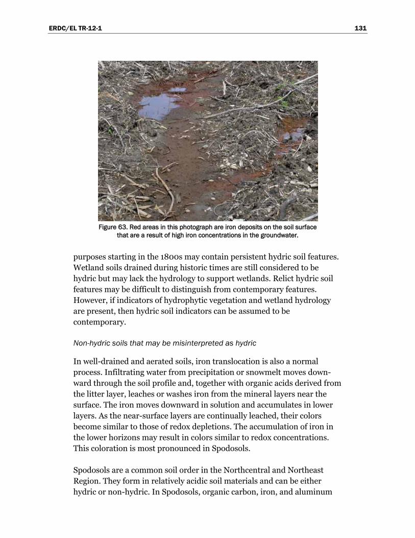
ERDC/EL TR-12-1 131
Figure 63. Red areas in this photograph are iron deposits on the soil surface
that are a result of high iron concentrations in the groundwater.
purposes starting in the 1800s may contain persistent hydric soil features. Wetland soils drained during historic times are still considered to be hydric but may lack the hydrology to support wetlands. Relict hydric soil features may be difficult to distinguish from contemporary features. However, if indicators of hydrophytic vegetation and wetland hydrology are present, then hydric soil indicators can be assumed to be contemporary.
Non-hydric soils that may be misinterpreted as hydric
In well-drained and aerated soils, iron translocation is also a normal process. Infiltrating water from precipitation or snowmelt moves down-ward through the soil profile and, together with organic acids derived from the litter layer, leaches or washes iron from the mineral layers near the surface. The iron moves downward in solution and accumulates in lower layers. As the near-surface layers are continually leached, their colors become similar to those of redox depletions. The accumulation of iron in the lower horizons may result in colors similar to redox concentrations. This coloration is most pronounced in Spodosols.
Spodosols are a common soil order in the Northcentral and Northeast Region. They form in relatively acidic soil materials and can be either hydric or non-hydric. In Spodosols, organic carbon, iron, and aluminum
ERDC/EL TR-12-1 132
are leached from a layer near the soil surface. This layer, known as the E horizon, has a bleached light-gray appearance and consists of relatively clean particles of sand and silt. The materials leached from the E horizon are deposited lower in the soil in the spodic horizon (e.g., Bhs or Bs horizon). If sufficient iron has been leached and redeposited, the spodic horizon will have a strong reddish color. In some Spodosols, E-horizon and spodic-horizon colors can be confused with the redox depletions and concentrations produced under anaerobic soil conditions. Normally, E horizons and spodic horizons are present in the soil in relatively con-tinuous horizontal bands. Chemical weathering in an aerated soil is accomplished by the downward movement of water; therefore, the layers or horizons are relatively parallel to the soil surface and consistent across the soil. Transitions are relatively abrupt between the organic-enriched surface, the leached E horizon, and the iron-enriched B horizon. Below the B horizon, the transition becomes more gradual as the red hue of the iron-enriched B horizon gradually changes to the yellower hue of the under-lying C horizon. However, if E horizons are thin or there are extensive plant roots, they may be discontinuous. Tree throw can also mix and break the horizons of aerated upland soils, so care should be taken to examine all site characteristics before concluding that a soil is hydric.
Generally, non-hydric Spodosols occur in the more mountainous portions of the region where temperatures are cooler. They tend to have thin, white-colored E horizons and spodic horizons that are less than 1 in. (2.5 cm) thick and not cemented. Hydric Spodosols are generally sandy in texture, have thicker gray-colored E horizons, and cemented spodic hori-zons (ortstein) that are greater than 1 in. (2.5 cm) thick.
Procedure
Soils that are thought to meet the definition of a hydric soil but do not exhibit any of the indicators described in Chapter 3 can be identified by the following recommended procedure. This procedure should be used only where indicators of hydrophytic vegetation and wetland hydrology are present (or are absent due to disturbance or other problem situations), but indicators of hydric soil are not evident.
1. Verify that one or more indicators of hydrophytic vegetation are present or that vegetation is problematic or has been altered (e.g., by tillage or other land alteration). If so, proceed to step 2.
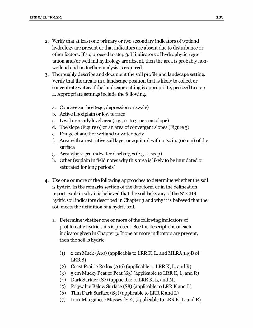
ERDC/EL TR-12-1 133
2. Verify that at least one primary or two secondary indicators of wetland hydrology are present or that indicators are absent due to disturbance or other factors. If so, proceed to step 3. If indicators of hydrophytic vege-tation and/or wetland hydrology are absent, then the area is probably non-wetland and no further analysis is required.
3. Thoroughly describe and document the soil profile and landscape setting. Verify that the area is in a landscape position that is likely to collect or concentrate water. If the landscape setting is appropriate, proceed to step 4. Appropriate settings include the following. a. Concave surface (e.g., depression or swale) b. Active floodplain or low terrace c. Level or nearly level area (e.g., 0- to 3-percent slope) d. Toe slope (Figure 6) or an area of convergent slopes (Figure 5) e. Fringe of another wetland or water body f. Area with a restrictive soil layer or aquitard within 24 in. (60 cm) of the
surface g. Area where groundwater discharges (e.g., a seep) h. Other (explain in field notes why this area is likely to be inundated or
saturated for long periods)
4. Use one or more of the following approaches to determine whether the soil is hydric. In the remarks section of the data form or in the delineation report, explain why it is believed that the soil lacks any of the NTCHS hydric soil indicators described in Chapter 3 and why it is believed that the soil meets the definition of a hydric soil. a. Determine whether one or more of the following indicators of
problematic hydric soils is present. See the descriptions of each indicator given in Chapter 3. If one or more indicators are present, then the soil is hydric. (1) 2 cm Muck (A10) (applicable to LRR K, L, and MLRA 149B of
LRR S) (2) Coast Prairie Redox (A16) (applicable to LRR K, L, and R) (3) 5 cm Mucky Peat or Peat (S3) (applicable to LRR K, L, and R) (4) Dark Surface (S7) (applicable to LRR K, L, and M) (5) Polyvalue Below Surface (S8) (applicable to LRR K and L) (6) Thin Dark Surface (S9) (applicable to LRR K and L) (7) Iron-Manganese Masses (F12) (applicable to LRR K, L, and R)
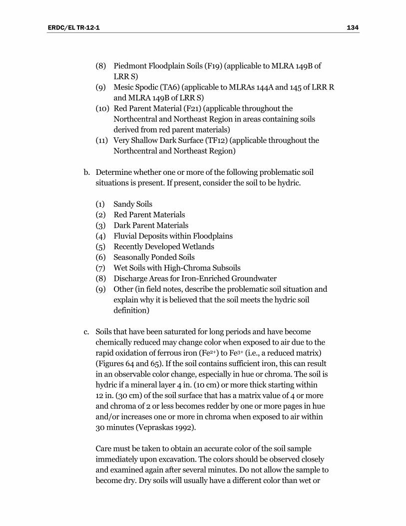
ERDC/EL TR-12-1 134
(8) Piedmont Floodplain Soils (F19) (applicable to MLRA 149B of LRR S)
(9) Mesic Spodic (TA6) (applicable to MLRAs 144A and 145 of LRR R and MLRA 149B of LRR S)
(10) Red Parent Material (F21) (applicable throughout the Northcentral and Northeast Region in areas containing soils derived from red parent materials)
(11) Very Shallow Dark Surface (TF12) (applicable throughout the Northcentral and Northeast Region)
b. Determine whether one or more of the following problematic soil situations is present. If present, consider the soil to be hydric. (1) Sandy Soils (2) Red Parent Materials (3) Dark Parent Materials (4) Fluvial Deposits within Floodplains (5) Recently Developed Wetlands (6) Seasonally Ponded Soils (7) Wet Soils with High-Chroma Subsoils (8) Discharge Areas for Iron-Enriched Groundwater (9) Other (in field notes, describe the problematic soil situation and
explain why it is believed that the soil meets the hydric soil definition)
c. Soils that have been saturated for long periods and have become chemically reduced may change color when exposed to air due to the rapid oxidation of ferrous iron (Fe2+) to Fe3+ (i.e., a reduced matrix) (Figures 64 and 65). If the soil contains sufficient iron, this can result in an observable color change, especially in hue or chroma. The soil is hydric if a mineral layer 4 in. (10 cm) or more thick starting within 12 in. (30 cm) of the soil surface that has a matrix value of 4 or more and chroma of 2 or less becomes redder by one or more pages in hue and/or increases one or more in chroma when exposed to air within 30 minutes (Vepraskas 1992). Care must be taken to obtain an accurate color of the soil sample immediately upon excavation. The colors should be observed closely and examined again after several minutes. Do not allow the sample to become dry. Dry soils will usually have a different color than wet or
ERDC/EL TR-12-1 135
moist soils. As always, do not attempt to determine colors while wearing sunglasses or tinted lenses. Colors must be determined in the field under natural light and not under artificial light.
Figure 64. This soil exhibits colors associated with
reducing conditions. Scale is 1 cm.
Figure 65. The same soil as in Figure 63 after
exposure to the air and oxidation has occurred.
d. If the soil is saturated at the time of sampling, alpha, alpha-dipyridyl reagent can be used in the following procedure to determine if reduced (ferrous) iron is present. If ferrous iron is present as described below, then the soil is hydric. Alpha, alpha-dipyridyl is a reagent that reacts with reduced iron. In some cases, it can be used to provide evidence that a soil is hydric when it lacks other hydric soil indicators. The soil is likely to be hydric if application of alpha, alpha-dipyridyl to mineral soil material in at least 60 percent of a layer at least 4 in. (10 cm) thick within a depth of 12 in. (30 cm) of the soil surface results in a positive reaction within 30 seconds evidenced by a pink or red coloration to the reagent during the growing season.
ERDC/EL TR-12-1 136
Using a dropper, apply a small amount of reagent to a freshly broken ped face to avoid any chance of a false positive test due to iron contami-nation from digging tools. Look closely at the treated soil for evidence of color change. If in doubt, apply the reagent to a sample of known upland soil and compare the reaction to the sample of interest. A positive reaction will not occur in soils that lack iron and may not occur in soils with high pH. The lack of a positive reaction to the reagent does not preclude the presence of a hydric soil. Specific information about the use of alpha, alpha-dipyridyl can be found in NRCS Hydric Soils Technical Note 8 (http://soils.usda.gov/use/hydric/ntchs/tech_notes/index.html).
e. Using gauge data, water-table monitoring data, or repeated direct hydrologic observations, determine whether the soil is ponded or flooded, or the water table is 12 in. (30 cm) or less from the surface, for 14 or more consecutive days during the growing season in most years (at least 5 years in 10, or 50 percent or higher probability) (U.S. Army Corps of Engineers 2005). If so, then the soil is hydric. Furthermore, any soil that meets the NTCHS hydric soil technical standard (NRCS Hydric Soils Technical Note 11, http://soils.usda.gov/use/hydric/ntchs/tech_notes/ index.html) is hydric.
Wetlands that periodically lack indicators of wetland hydrology
Description of the problem
Wetlands are areas that are flooded or ponded, or have soils that are saturated with water, for long periods during the growing season in most years. If the site is visited during a time of normal precipitation amounts and it is inundated or the water table is near the surface, then the wetland hydrology determination is straight forward. During the dry season, how-ever, surface water recedes from wetland margins, water tables drop, and many wetlands dry out completely. Superimposed on this seasonal cycle is a long-term pattern of multi-year droughts alternating with years of higher-than-average rainfall. Wetlands in general are inundated or satu-rated at least 5 years in 10 (50 percent or higher probability) over a long-term record. However, some wetlands in the Northcentral and Northeast Region do not become inundated or saturated in some years and, during drought cycles or prolonged dry conditions, may not inundate or saturate for several years in a row.
ERDC/EL TR-12-1 137
Wetland hydrology determinations are based on indicators, many of which were designed to be used during dry periods when the direct observation of surface water or a shallow water table is not possible. However, some wetlands may lack any of the listed hydrology indicators, particularly during the dry season or in a dry year. Examples in the region include vernal pools and potholes, floodplain wetlands, flatwoods, interdunal swales, wet prairies, sedge meadows, and other wet meadows. The evalu-ation of wetland hydrology requires special care on any site where indi-cators of hydrophytic vegetation and hydric soil are present but hydrology indicators appear to be absent. Among other factors, this evaluation should consider the timing of the site visit in relation to normal seasonal and annual hydrologic variability, and whether the amount of rainfall prior to the site visit has been normal. This section describes a number of approaches that can be used to determine whether wetland hydrology is present on sites where indicators of hydrophytic vegetation and hydric soil are present but hydrology indicators may be lacking due to normal vari-ations in rainfall or runoff, human activities that destroy hydrology indi-cators, and other factors.
Procedure
1. Verify that indicators of hydrophytic vegetation and hydric soil are present, or are absent due to disturbance or other problem situations. If so, proceed to step 2.
2. Verify that the site is in a landscape position that is likely to collect or con-centrate water. If the landscape setting is appropriate, proceed to step 3. Appropriate settings are listed below. a. Concave surface (e.g., depression or swale) b. Active floodplain or low terrace c. Level or nearly level area (e.g., 0- to 3-percent slope) d. Toe slope (Figure 6) or an area of convergent slopes (Figure 5) e. Fringe of another wetland or water body f. Area with a restrictive soil layer or aquitard within 24 in. (60 cm) of the
surface g. Area where groundwater discharges (e.g., a seep) h. Other (explain in field notes why this area is likely to be inundated or
saturated for long periods)
3. Use one or more of the following approaches to determine whether wet-land hydrology is present and the site is a wetland. In the remarks section
ERDC/EL TR-12-1 138
of the data form or in the delineation report, explain the rationale for concluding that wetland hydrology is present even though indicators of wetland hydrology described in Chapter 4 were not observed. a. Site visits during the dry season. Determine whether the site visit
occurred during the normal annual “dry season.” The dry season, as used in this supplement, is the period of the year when soil moisture is normally being depleted and water tables are falling to low levels in response to decreased precipitation and/or increased evapotranspira-tion, usually during late spring and summer. It also includes the beginning of the recovery period in late summer or fall. The Web-Based Water-Budget Interactive Modeling Program (WebWIMP) is one source for approximate dates of wet and dry seasons for any ter-restrial location based on average monthly precipitation and estimated evapotranspiration (http://climate.geog.udel.edu/~wimp/). In general, the dry season in a typical year is indicated when potential evapotranspiration exceeds precipitation (indicated by negative values of DIFF in the WebWIMP output), resulting in drawdown of soil moisture storage (negative values of DST) and/or a moisture deficit (positive values of DEF, also called the unmet atmospheric demand for moisture). Actual dates for the dry season vary by locale and year. In many wetlands, direct observation of flooding, ponding, or a shallow water table would be unexpected during the dry season. Wetland hydrology indicators, if present, would most likely be limited to indirect evidence, such as water marks, drift deposits, or surface cracks. In some situations, hydrology indicators may be absent during the dry season. If the site visit occurred during the dry season on a site that contains hydric soils and hydrophytic vegetation and no signifi-cant hydrologic manipulation (e.g., no dams, levees, water diversions, land grading, etc., and the site is not within the zone of influence of any ditches or subsurface drains), then consider the site to be a wetland. If necessary, revisit the site during the normal wet season and check again for the presence or absence of wetland hydrology indicators, or use one or more of the following evaluation methods.
b. Periods with below-normal rainfall. Determine whether the amount of rainfall that occurred in the 2 to 3 months preceding the site visit was normal, above normal, or below normal based on the normal range reported in WETS tables. WETS tables are provided by the
ERDC/EL TR-12-1 139
NRCS National Water and Climate Center (http://www.wcc.nrcs.usda.gov/climate/ wetlands.html) and are calculated from long-term (30-year) weather records gathered at National Weather Service meteorological stations. To determine whether precipitation was normal prior to the site visit, actual rainfall in the current month and previous 2 to 3 months should be compared with the normal ranges for each month given in the WETS table (USDA Natural Resources Conservation Service 1997, Sprecher and Warne 2000). The lower and upper limits of the normal range are indicated by the columns labeled “30% chance will have less than” and “30% chance will have more than” in the WETS table. The USDA Natural Resources Conservation Service (1997, Section 650.1903) also gives a procedure that can be used to weight the infor-mation from each month and determine whether the entire period was normal, wet, or dry. When precipitation has been below normal, wetlands may not flood, pond, or develop shallow water tables even during the typical wet por-tion of the growing season and may not exhibit other indicators of wet-land hydrology. Therefore, if precipitation was below normal prior to the site visit, and the site contains hydric soils and hydrophytic vege-tation and no significant hydrologic manipulation (e.g., no dams, levees, water diversions, land grading, etc., and the site is not within the zone of influence of any ditches or subsurface drains), then con-sider the site to be a wetland. If necessary, revisit the site during a period of normal rainfall and check again for hydrology indicators, or use one or more of the other evaluation methods described in this section.
c. Drought years. Determine whether the area has been subject to drought. Drought periods can be identified by comparing annual rainfall totals with the normal range of annual rainfall given in WETS tables or by examining trends in drought indices, such as the Palmer Drought Severity Index (PDSI) (Sprecher and Warne 2000). PDSI takes into account not only precipitation but also temperature, which affects evapotranspiration, and soil moisture conditions. The index is usually calculated on a monthly basis for major climatic divisions within each state. Therefore, the information is not site-specific. PDSI ranges potentially between –6 and +6 with negative values indicating dry periods and positive values indicating wet periods. An index of -1.0 indicates mild drought, –2.0 indicates moderate drought, -3.0 indicates severe drought, and –4.0 indicates extreme drought.
ERDC/EL TR-12-1 140
Time-series plots of PDSI values by month or year are available from the National Climatic Data Center at (http://www.ncdc.noaa.gov/oa/climate/ onlineprod/drought/xmgr.html#ds). If wetland hydrology indicators appear to be absent on a site that has hydrophytic vegetation and hydric soils, no significant hydrologic manipulation (e.g., no dams, levees, water diver-sions, land grading, etc., and the site is not within the zone of influence of any ditches or subsurface drains), and the region has been affected by drought, then consider the site to be a wetland. If necessary, revisit the site during a normal rainfall year and check again for wetland hydrology indicators, or use one or more of the other methods described in this section.
d. Reference sites. If indicators of hydric soil and hydrophytic vegetation are present on a site that lacks wetland hydrology indicators, the site may be considered to be a wetland if the landscape setting, topography, soils, and vegetation are substantially the same as those on nearby wet-land reference areas with known hydrology. Hydrology of wetland reference areas should be documented through long-term monitoring (see item g below) or by application of the procedure described in item 5b on page 132 (Direct Hydrologic Observations) of the procedure for Problematic Hydrophytic Vegetation in this chapter. Reference sites should be minimally disturbed and provide long-term access. Soils, vegetation, and hydrologic conditions should be thoroughly documented and the data kept on file in the District or field office.
e. Hydrology tools. The “Hydrology Tools” (USDA Natural Resources Conservation Service 1997) is a collection of methods that can be used to determine whether wetland hydrology is present on a potential wetland site that lacks indicators due to disturbance or other reasons, particularly on lands used for agriculture. Generally they require addi-tional information, such as aerial photographs or stream-gauge data, or involve hydrologic modeling and approximation techniques. These methods are not intended to overrule an indicator-based wetland determination on a site that is not disturbed or problematic. A hydrolo-gist may be needed to help select and carry out the proper analysis. The seven hydrology tools are used to: (1) Analyze stream and lake gauge data
ERDC/EL TR-12-1 141
(2) Estimate runoff volumes and determine duration and frequency of ponding in depressional areas, based on precipitation and tempera-ture data, soil characteristics, land cover, and other inputs
(3) Evaluate the frequency of wetness signatures on repeated aerial photography (see item f below for additional information)
(4) Model water-table fluctuations in fields with parallel drainage systems using the DRAINMOD model
(5) Estimate the “scope and effect” of ditches or subsurface drain lines (6) Use NRCS state drainage guides to estimate the effectiveness of
agricultural drainage systems (7) Analyze data from groundwater monitoring wells (see item g below
for additional information)
f. Evaluating multiple years of aerial photography. Each year, the Farm Service Agency (FSA) takes low-level aerial photographs in agricultural areas to monitor the acreages planted in various crops for USDA pro-grams. NRCS has developed an off-site procedure that uses these photos, or repeated aerial photography from other sources, to make wetland hydrology determinations (USDA Natural Resources Conser-vation Service 1997, Section 650.1903). The method is intended for use on agricultural lands where human activity has altered or destroyed other wetland indicators. However, the same approach may be useful in other environments. The procedure uses five or more years of growing-season photography and evaluates each photo for wetness signatures that are listed in “wetland mapping conventions” developed by NRCS state offices. Wetland mapping conventions can be found in the electronic Field Office Technical Guide (eFOTG) for each state (http://www.nrcs.usda.gov/ technical/efotg/). From the national web site, choose the appropriate state, then select any county (the state’s wetland mapping conventions are the same in every county). Wetland mapping conventions are listed among the references in Section I of the eFOTG. However, not all states have wetland mapping conventions. Wetness signatures for a particular state may include surface water, saturated soils, flooded or drowned-out crops, stressed crops due to wetness, differences in vegetation patterns due to different planting dates, inclusion of wet areas into set-aside programs, unharvested crops, isolated areas that are not farmed with the rest of the field,
ERDC/EL TR-12-1 142
patches of greener vegetation during dry periods, and other evidence of wet conditions (see Part 513.30 of USDA Natural Resources Conserva-tion Service 1994). For each photo, the procedure described in item b above is used to determine whether the amount of rainfall in the 2 to 3 months prior to the date of the photo was normal, below normal, or above normal. Only photos taken in normal rainfall years, or an equal number of wetter-than-normal and drier-than-normal years, are used in the analysis. If wetness signatures are observed on photos in more than half of the years included in the analysis, then wetland hydrology is present. Data forms that may be used to document the wetland hydrology determination are given in section 650.1903 of USDA Natural Resources Conservation Service (1997).
g. Long-term hydrologic monitoring. On sites where the hydrology has been manipulated by man (e.g., with ditches, subsurface drains, dams, levees, water diversions, land grading) or where natural events (e.g., downcutting of streams) have altered conditions such that hydrology indicators may be missing or misleading, direct monitoring of surface and groundwater may be needed to determine the presence or absence of wetland hydrology. The U. S. Army Corps of Engineers (2005) provides minimum standards for the design, construction, and installa-tion of water-table monitoring wells, and for the collection and inter-pretation of groundwater monitoring data, in cases where direct hydrologic measurements are needed to determine whether wetlands are present on highly disturbed or problematic sites. This standard calls for 14 or more consecutive days of flooding, ponding, or a water table 12 in. (30 cm) or less below the soil surface during the growing season at a minimum frequency of 5 years in 10 (50 percent or higher probability), unless a different standard has been established for a particular geographic area or wetland type. A disturbed or problematic site that meets this standard has wetland hydrology. This standard is not intended (1) to overrule an indicator-based wetland determination on a site that is not disturbed or problematic, or (2) to test or validate existing or proposed wetland indicators.
Wetland/non-wetland mosaics
Description of the problem
In this supplement, “mosaic” refers to a landscape where wetland and non-wetland components are too closely associated to be easily delineated or
ERDC/EL TR-12-1 143
mapped separately. These areas often have complex microtopography, with repeated small changes in elevation occurring over short distances. Tops of ridges and hummocks are often non-wetland but are interspersed throughout a wetland matrix having clearly hydrophytic vegetation, hydric soils, and wetland hydrology. Potential examples of wetland/non-wetland mosaics in the Northcentral and Northeast Region include ridge-and-swale topography on floodplains; dune-and-swale systems near the Great Lakes and Atlantic coast; current and former flatwoods, such as those on the Lake Superior clay plain in northeastern Minnesota and northern Wisconsin; areas that exhibit bedding from agricultural or silvicultural operations; areas containing numerous vernal pools; and areas where wind-thrown trees have created pit-and-mound or cradle/knoll topography.
Wetland components of a mosaic are often not difficult to identify. The problem for the wetland delineator is that microtopographic features are too small and intermingled, and there are too many such features per acre, to delineate and map them accurately. Instead, the following sampling approach can be used to estimate the percentage of wetland in the mosaic. From this, the number of acres of wetland on the site can be calculated, if needed.
Procedure
First, identify and flag all contiguous areas of either wetland or non-wetland on the site that are large enough to be delineated and mapped separately. The remaining area should be mapped as “wetland/non-wetland mosaic” and the approximate percentage of wetland within the area determined by the following procedure.
1. Establish one or more continuous line transects across the mosaic area, as needed. Measure the total length of each transect. A convenient method is to stretch a measuring tape along the transect and leave it in place while sampling. If the site is shaped appropriately and multiple transects are used, they should be arranged in parallel with each transect starting from a random point along one edge of the site. However, other arrangements of transects may be needed for oddly shaped sites.
2. Use separate data forms for the swales or troughs and for the ridges or hummocks. Sampling of vegetation, soil, and hydrology should follow the general procedures described in the Corps Manual and this supplement. Plot sizes and shapes for vegetation sampling must be adjusted to fit the microtopographic features on the site. Plots intended to sample the
ERDC/EL TR-12-1 144
troughs should not overlap adjacent hummocks, and vice versa. Only one or two data forms are required for each microtopographic position, and do not need to be repeated for similar features or plant communities.
3. Identify every wetland boundary in every trough or swale encountered along each transect. Each boundary location may be marked with a pin flag or simply recorded as a distance along the stretched tape.
4. Determine the total distance along each transect that is occupied by wet-lands and non-wetlands until the entire length of the line has been accounted for. Sum these distances across transects, if needed. Determine the percentage of wetland in the wetland/non-wetland mosaic by the following formula.
%Total wetland distance along all transects
wetlandTotal length of all transects
100
An alternative approach involves point-intercept sampling at fixed inter-vals along transects across the area designated as wetland/non-wetland mosaic. This method avoids the need to identify wetland boundaries in each swale, and can be carried out by pacing rather than stretching a measuring tape across the site. The investigator uses a compass or other means to follow the selected transect line. At a fixed number of paces (e.g., every two steps) the wetland status of that point is determined by observing indicators of hydrophytic vegetation, hydric soil, and wetland hydrology. Again, a completed data form is not required at every point but at least one representative swale and hummock should be documented with completed forms. After all transects have been sampled, the result is a number of wetland sampling points and a number of non-wetland points. Estimate the percentage of wetland in the wetland/non-wetland mosaic by the following formula:
Number of wetland points along all transectswetland
Total number of points sampled along all transects% 100
If high-quality aerial photography is available for the site, a third approach to estimating the percentage of wetland in a wetland/non-wetland mosaic is to use a dot grid, planimeter, or geographic information system (GIS) to determine the percentage of ridges (non-wetlands) and swales (wetlands) through photo interpretation of topography and vegetation patterns. This technique requires onsite verification that most ridges qualify as non-wetlands and most swales qualify as wetlands.
ERDC/EL TR-12-1 145
References Bailey, R. G. 1995. Description of the ecoregions of the United States, second edition.
Miscellaneous Publication 1391 (revised). Washington, DC: U.S. Department of Agriculture, Forest Service. (http://www.fs.fed.us/land/ecosysmgmt/ecoreg1_home.html)
Barbour, M. G., and W. D. Billings, eds. 1988. North American terrestrial vegetation. New York, NY: Cambridge University Press.
Barbour, M. G., J. H. Burk, W. D. Pitts, F. S. Gilliam, and M. W. Schwartz. 1999. Terrestrial plant ecology, 3rd edition. Toronto, Canada: Addison Wesley.
Barkley, T. M., ed. 1986. Flora of the Great Plains. Lawrence, KS: University Press of Kansas.
Braun, E. L. 1950. Deciduous forests of eastern North America. Philadelphia, PA: Blakiston.
Brohman, R. J., and L. D. Bryant, eds. 2005. Existing vegetation classification and mapping technical guide, version 1.0. General Technical Report WO-67. Washington, DC: U.S. Department of Agriculture, Forest Service.
Carr, D. W., D. A. Leeper, and T. F. Rochow. 2006. Comparison of six biologic indicators of hydrology and the landward extent of hydric soils in west-central Florida, USA, cypress domes. Wetlands 26:1012–1019.
Colburn, E. A. 2004. Vernal pools: Natural history and conservation. Blacksburg, VA: McDonald and Woodward.
Cox, G. 1990. Laboratory manual of general ecology, sixth edition. Dubuque, IA: William C. Brown.
Curtis, J. 1971. The vegetation of Wisconsin. Madison, WI: University of Wisconsin Press.
Davis, M. B. 1981. Quaternary history and the stability of forest communities. In Forest succession: Concepts and application, ed. D. C. West, H. H. Shugart, and D. B. Botkin, 132–153. New York, NY: Springer-Verlag.
Eggers, S., and D. Reed. 1997. Wetland plants and plant communities of Minnesota and Wisconsin. St. Paul, MN: St. Paul District, U.S. Army Corps of Engineers.
Embleton, C., and C. A. M. King. 1968. Glacial and periglacial geomorphology. New York, NY: St. Martin’s Press.
Environmental Laboratory. 1987. Corps of Engineers wetlands delineation manual. Technical Report Y-87-1. Vicksburg, MS: U.S. Army Engineer Waterways Experiment Station. (http://el.erdc.usace.army.mil/wetlands/pdfs/wlman87.pdf)
Foster, D. R., and G. A. King. 1984. Landscape features, vegetation and developmental history of a patterned fen in south-eastern Labrador, Canada. Journal of Ecology 72: 115-143.
ERDC/EL TR-12-1 146
Frankenberger, J., E. Kladivko, G. Sands, D. Jaynes, N. Fausey, M. Helmers, R. Cooke, J. Strock, K. Nelson, and L. Brown. 2006. Questions and answers about drainage water management for the Midwest. Report WQ-44. West Lafayette, IN: Purdue University Cooperative Extension Service. (http://www.ces.purdue.edu/extmedia/WQ/WQ-44.pdf)
Freeze, R. A. and J. A. Cherry. 1979. Groundwater. Englewood Cliffs, NJ: Prentice-Hall.
Gretag/Macbeth. 2000. Munsell® color. New Windsor, NY.
Johnson, C. 1985. Bogs of the Northeast. Hanover, NH: University Press of New England.
Kent, M., and P. Coker. 1992. Vegetation description and analysis: A practical approach. New York, NY: Wiley.
Maine Geological Survey. 2005. Surficial geologic history of Maine. Augusta, ME. http://maine.gov/doc/nrimc/mgs/explore/surficial/facts/surficial.htm; accessed 9 May 2008.
Martini, I. P., M. E. Brookfield, and S. Sadura. 2001. Principles of glacial geomorphology and geology. Upper Saddle River, NJ: Prentice-Hall.
Megonigal, J. P., S. P. Faulkner, and W. H. Patrick. 1996. The microbial activity season in southeastern hydric soils. Soil Science Society of America Journal 60:1263–1266.
Metzler, K., and R. W. Tiner. 1992. Wetlands of Connecticut. Report of Investigations No. 13. Hartford, CT: State Geological and Natural History Survey of Connecticut, Department of Environmental Protection.
Minnesota Department of Natural Resources. 2003. Field guide to the native plant communities of Minnesota: The Laurentian mixed forest province. St. Paul, MN: Ecological Land Classification Program, Minnesota County Biological Survey, and Natural Heritage and Nongame Research Program.
Mueller-Dombois, D., and H. Ellenberg. 1974. Aims and methods of vegetation ecology. New York, NY: Wiley.
National Research Council. 1995. Wetlands: Characteristics and boundaries. Washington, DC: National Academy Press.
Rabenhorst, M.C. and S. Parikh. 2000. Propensity of soils to develop redoximorphic color changes. Soil Science Society of America Journal 64:1904-1910.
Reed, P. B., Jr. 1988. National list of plant species that occur in wetlands: 1988 national summary. Biological Report 88(24). Washington, DC: U.S. Fish and Wildlife Service. (http://www.usace.army.mil/CECW/Documents/cecwo/reg/plants/list88.pdf)
Reschke, C. 1990. Ecological communities of New York State. Latham, NY: New York State Natural Heritage Program, Department of Environmental Conservation.
Russell, E. W. B. 1983. Indian-set fires in the forests of the northeastern United States. Ecology 64:78–88.
ERDC/EL TR-12-1 147
Sperduto, D. D. 2005. Natural community systems of New Hampshire. Concord, NH: New Hampshire Natural Heritage Bureau and The Nature Conservancy.
Sprecher, S. W., and A. G. Warne. 2000. Accessing and using meteorological data to evaluate wetland hydrology. ERDC/EL TR-WRAP-00-1. Vicksburg, MS: U.S. Army Engineer Research and Development Center. (http://el.erdc.usace.army.mil/elpubs/pdf/wrap00-1/wrap00-1.pdf)
Stein, B. A., L. S. Kutner, and J. S. Adams. 2000. Precious heritage: The status of biodiversity in the United States. New York, NY: Oxford University Press.
Stolt, M. H., B. C. Lesinski, and W. Wright. 2001. Micromorphology of seasonally saturated soils in carboniferous glacial till. Soil Science 166:406–414.
Stone, J., and G. M. Ashley. 1992. Ice-wedge casts, pingo scars, and the drainage of glacial Lake Hitchcock. In 84th annual meeting of the New England intercollegiate geological conference: Guidebook for field trips in the Connecticut Valley region of Massachusetts and adjacent states, 305–331. Amherst, MA: University of Massachusetts, Department of Geology and Geography.
Stuckey, R. L., and T. M. Barkley. 1993. Weeds in North America. Vol. 1, Chapter 8 in Flora of North America north of Mexico, ed. Flora of North America Editorial Committee. New York, NY: Oxford University Press.
Tiner, R. W. 1989. Wetlands of Rhode Island. Newton Corner, MA: U.S. Fish and Wildlife Service, Northeast Region.
Tiner, R. W. 1999. Wetland indicators: A guide to wetland identification, delineation, classification, and mapping. Boca Raton, FL: Lewis Publishers.
Tiner, R. W. 2005. In search of swampland: A wetland sourcebook and field guide, second edition. New Brunswick, NJ: Rutgers University Press.
Tiner, R. W. 2008. Field guide to tidal wetland plants of the northeastern United States and neighboring Canada. Amherst, MA: University of Massachusetts Press.
U. S. Army Corps of Engineers. 2005. Technical standard for water-table monitoring of potential wetland sites. ERDC TN-WRAP-05-02. Vicksburg, MS: U.S. Army Engineer Research and Development Center. (http://el.erdc.usace.army.mil/wrap/pdf/tnwrap05-2.pdf)
USDA Natural Resources Conservation Service. 1994. National food security act manual, third edition (as amended). Washington, DC. (http://www.nrcs.usda.gov/programs/compliance/index.html)
USDA Natural Resources Conservation Service. 1997. Hydrology tools for wetland determination. Chapter 19, Engineering Field Handbook. Fort Worth, TX: U.S. Department of Agriculture. (http://policy.nrcs.usda.gov/OpenNonWebContent.aspx?content=17556.wba)
USDA Natural Resources Conservation Service. 1999. Soil taxonomy: A basic system of soil classification for making and interpreting soil surveys. Agriculture Handbook 436. Washington, DC: U.S. Department of Agriculture. (http://soils.usda.gov/technical/classification/taxonomy/)
ERDC/EL TR-12-1 148
USDA Natural Resources Conservation Service. 2002. Field book for describing and sampling soils, version 2.0. ed. P. J. Schoeneberger, D. A. Wysocki, E. C. Benham, and W. D. Broderson. Lincoln, NE: National Soil Survey Center. (http://soils.usda.gov/technical/fieldbook/)
USDA Natural Resources Conservation Service. 2005. National soil survey handbook, part 629, glossary. Washington, DC: U.S. Department of Agriculture. (ftp://ftp-fc.sc.egov.usda.gov/NSSC/Soil_Survey_Handbook/629_glossary.pdf)
USDA Natural Resources Conservation Service. 2006. Land resource regions and major land resource areas of the United States, the Caribbean, and the Pacific Basin. Agriculture Handbook 296. Washington, DC: U.S. Department of Agriculture. (http://soils.usda.gov/survey/geography/mlra/index.html)
USDA Natural Resources Conservation Service. 2010. Field indicators of hydric soils in the United States, Version 7.0. ed. L. M. Vasilas, G. W. Hurt, and C. V. Noble. Washington, DC: USDA NRCS in cooperation with the National Technical Committee for Hydric Soils. (http://soils.usda.gov/use/hydric/)
USDA Soil Conservation Service. 1994. Changes in hydric soils of the United States. Federal Register 59(133):35680–35681, July 13, 1994.
U.S. Department of the Interior (USDI) Bureau of Land Management. 1996. Sampling vegetation attributes. BLM/RS/ST-96/002+1730. Denver, CO.
Vepraskas, M. J. 1992. Redoximorphic features for identifying aquic conditions. Technical Bulletin 301. Raleigh, NC: North Carolina Agricultural Research Service, North Carolina State Univ.
Vepraskas, M. J., and S. W. Sprecher 1997. Aquic conditions and hydric soils: The problem soils. Special Publication Number 50. Madison, WI: Soil Science Society of America.
Wakeley, J. S., and R. W. Lichvar. 1997. Disagreement between plot-based prevalence indices and dominance ratios in evaluations of wetland vegetation. Wetlands 17:301–309.
Wentworth, T. R., G. P. Johnson, and R. L. Kologiski. 1988. Designation of wetlands by weighted averages of vegetation data: A preliminary evaluation. Water Resources Bulletin 24:389–396.
Wright, H., B. Coffin, and N. Aaseng, eds. 1992. The patterned peatlands of Minnesota. Minneapolis, MN: University of Minnesota Press.
ERDC/EL TR-12-1 149
Appendix A: Glossary
This glossary is intended to supplement those given in the Corps Manual and other available sources. See the following publications for terms not listed here:
• Corps Manual (Environmental Laboratory 1987) (http://el.erdc.usace.army.mil/wetlands/pdfs/wlman87.pdf).
• Field Indicators of Hydric Soils in the United States (USDA Natural Resources Conservation Service 2010) (http://soils.usda.gov/use/hydric/).
• National Soil Survey Handbook, Part 629 (USDA Natural Resources Conservation Service 2005) (ftp://ftp-fc.sc.egov.usda.gov/NSSC/Soil_Survey_Handbook/629_glossary.pdf).
Absolute cover. In vegetation sampling, the percentage of the ground surface that is covered by the aerial portions (leaves and stems) of a plant species when viewed from above. Due to overlapping plant canopies, the sum of absolute cover values for all species in a community or stratum may exceed 100 percent. In contrast, “relative cover” is the absolute cover of a species divided by the total coverage of all species in that stratum, expressed as a percent. Relative cover cannot be used to calculate the prevalence index.
Aquitard. A layer of soil or rock that retards the downward flow of water and is capable of perching water above it. For the purposes of this supple-ment, the term aquitard also includes the term aquiclude, which is a soil or rock layer that is incapable of transmitting significant quantities of water under ordinary hydraulic gradients.
Contrast. The color difference between a redox concentration and the dominant matrix color. Differences are classified as faint, distinct, or prominent and are defined in the glossary of USDA Natural Resources Conservation Service (2010) and illustrated in Table A1.
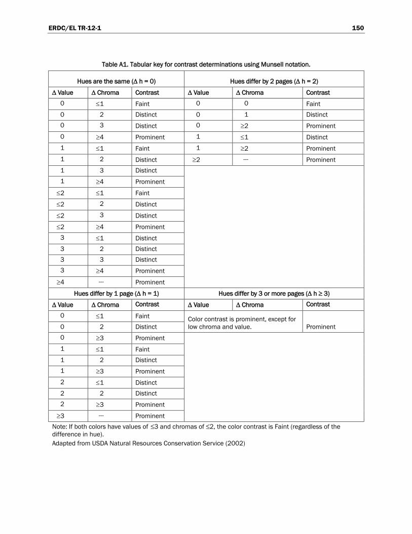
ERDC/EL TR-12-1 150
Table A1. Tabular key for contrast determinations using Munsell notation.
Hues are the same (∆ h = 0) Hues differ by 2 pages (∆ h = 2)
∆ Value ∆ Chroma Contrast ∆ Value ∆ Chroma Contrast 0 ≤1 Faint 0 0 Faint 0 2 Distinct 0 1 Distinct 0 3 Distinct 0 ≥2 Prominent 0 ≥4 Prominent 1 ≤1 Distinct 1 ≤1 Faint 1 ≥2 Prominent 1 2 Distinct ≥2 --- Prominent 1 3 Distinct 1 ≥4 Prominent
≤2 ≤1 Faint
≤2 2 Distinct
≤2 3 Distinct
≤2 ≥4 Prominent 3 ≤1 Distinct 3 2 Distinct 3 3 Distinct 3 ≥4 Prominent
≥4 --- Prominent
Hues differ by 1 page (∆ h = 1) Hues differ by 3 or more pages (∆ h ≥ 3)
∆ Value ∆ Chroma Contrast ∆ Value ∆ Chroma Contrast
0 ≤1 Faint Color contrast is prominent, except for low chroma and value. Prominent 0 2 Distinct
0 ≥3 Prominent
1 ≤1 Faint 1 2 Distinct 1 ≥3 Prominent 2 ≤1 Distinct 2 2 Distinct 2 ≥3 Prominent
≥3 --- Prominent Note: If both colors have values of ≤3 and chromas of ≤2, the color contrast is Faint (regardless of the difference in hue). Adapted from USDA Natural Resources Conservation Service (2002)
ERDC/EL TR-12-1 151
Depleted matrix. The volume of a soil horizon or subhorizon from which iron has been removed or transformed by processes of reduction and translocation to create colors of low chroma and high value. A, E, and calcic horizons may have low chromas and high values and may therefore be mistaken for a depleted matrix. However, they are excluded from the concept of depleted matrix unless common or many, distinct or prominent redox concentrations as soft masses or pore linings are present. In some places the depleted matrix may change color upon exposure to air (reduced matrix); this phenomenon is included in the concept of depleted matrix. The following combinations of value and chroma identify a depleted matrix:
• Matrix value of 5 or more and chroma of 1, with or without redox con-centrations occurring as soft masses and/or pore linings, or
• Matrix value of 6 or more and chroma of 2 or 1, with or without redox concentrations occurring as soft masses and/or pore linings, or
• Matrix value of 4 or 5 and chroma of 2, with 2 percent or more distinct or prominent redox concentrations occurring as soft masses and/or pore linings, or
• Matrix value of 4 and chroma of 1, with 2 percent or more distinct or prominent redox concentrations occurring as soft masses and/or pore linings (USDA Natural Resources Conservation Service 2010).
Common (2 to less than 20 percent) to many (20 percent or more) redox concentrations (USDA Natural Resources Conservation Service 2002) are required in soils with matrix colors of 4/1, 4/2, and 5/2 (Figure A1). Redox concentrations include iron and manganese masses and pore linings (Vepraskas 1992). See “contrast” in this glossary for the definitions of “distinct” and “prominent.”
Diameter at breast height (DBH). A standard method of expressing the diameter of the trunk or bole measured at 1.37 meters (4.5 ft) above the ground. On sloping ground, measurements should be taken from the uphill side of the trunk.
Diapause. A period during which growth or development is suspended and physiological activity is diminished, as in certain aquatic invertebrates in response to drying of temporary wetlands.
Distinct. See Contrast.
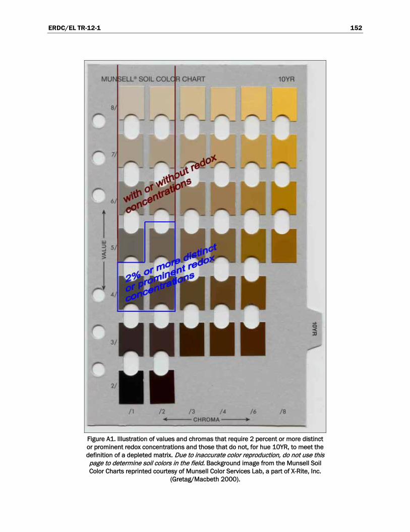
ERDC/EL TR-12-1 152
Figure A1. Illustration of values and chromas that require 2 percent or more distinct or prominent redox concentrations and those that do not, for hue 10YR, to meet the definition of a depleted matrix. Due to inaccurate color reproduction, do not use this page to determine soil colors in the field. Background image from the Munsell Soil Color Charts reprinted courtesy of Munsell Color Services Lab, a part of X-Rite, Inc.
(Gretag/Macbeth 2000).
ERDC/EL TR-12-1 153
Episaturation. Condition in which the soil is saturated with water at or near the surface, but also has one or more unsaturated layers below the saturated zone. The zone of saturation is perched on top of a relatively impermeable layer.
Flark-and-strang topography. Microtopographic relief consisting of flarks (linear pools or swales) and strangs or strings (low ridges) oriented perpendicular to the direction of water flow in patterned fens, bogs, and other peatlands (Foster and King 1984).
Fragmental soil material. Soil material that consists of 90 percent or more rock fragments; less than 10 percent of the soil consists of particles 2 mm or smaller (USDA Natural Resources Conservation Service 2010).
Gleyed matrix. A gleyed matrix has one of the following combinations of hue, value, and chroma and the soil is not glauconitic (Figure A2):
• 10Y, 5GY, 10GY, 10G, 5BG, 10BG, 5B, 10B, or 5PB with value of 4 or more and chroma of 1; or
• 5G with value of 4 or more and chroma of 1 or 2; or • N with value of 4 or more (USDA Natural Resources Conservation
Service 2010).
Growing season. In the Northcentral and Northeast Region, growing season dates are determined through onsite observations of the following indicators of biological activity in a given year: (1) above-ground growth and development of vascular plants and/or (2) soil temperature (see Chapter 4 for details). If onsite data gathering is not practical, growing season dates may be approximated by using WETS tables available from the NRCS National Water and Climate Center to determine the median dates of 28 °F (−2.2 °C) air temperatures in spring and fall based on long-term records gathered at the nearest appropriate National Weather Service meteorological station.
High pH. pH of 7.9 or higher. Includes Moderately Alkaline, Strongly Alkaline, and Very Strongly Alkaline (USDA Natural Resources Conser-vation Service 2002).
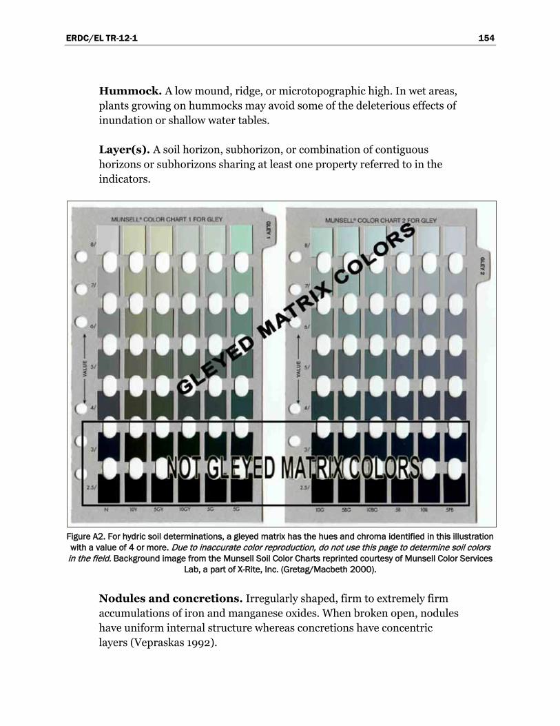
ERDC/EL TR-12-1 154
Hummock. A low mound, ridge, or microtopographic high. In wet areas, plants growing on hummocks may avoid some of the deleterious effects of inundation or shallow water tables.
Layer(s). A soil horizon, subhorizon, or combination of contiguous horizons or subhorizons sharing at least one property referred to in the indicators.
Figure A2. For hydric soil determinations, a gleyed matrix has the hues and chroma identified in this illustration with a value of 4 or more. Due to inaccurate color reproduction, do not use this page to determine soil colors
in the field. Background image from the Munsell Soil Color Charts reprinted courtesy of Munsell Color Services Lab, a part of X-Rite, Inc. (Gretag/Macbeth 2000).
Nodules and concretions. Irregularly shaped, firm to extremely firm accumulations of iron and manganese oxides. When broken open, nodules have uniform internal structure whereas concretions have concentric layers (Vepraskas 1992).
ERDC/EL TR-12-1 155
Ped. A unit of soil structure, such as a block, column, granule, plate, or prism, formed by natural processes.
Prominent. See Contrast.
Red parent material. Parent material with a natural inherent reddish color attributable to the presence of iron oxides occurring as coatings on and occluded within the mineral grains. Soils that formed in red parent material have conditions that greatly retard the development and extent of the redoximorphic features that normally occur under prolonged aquic conditions. Most commonly, the material consists of dark red, consolidated Mesozoic or Paleozoic sedimentary rocks, such as shale, siltstone, and sandstone, or alluvial materials derived from such rocks. Assistance from a local soil scientist may be needed to determine where red parent material occurs.
Reduced matrix. Soil matrix that has a low chroma in situ due to presence of reduced iron, but whose color changes in hue or chroma when exposed to air as Fe2+ is oxidized to Fe3+ (Vepraskas 1992).
Saturation. For wetland delineation purposes, a soil layer is saturated if virtually all pores between soil particles are filled with water (National Research Council 1995, Vepraskas and Sprecher 1997). This definition includes part of the capillary fringe above the water table (i.e., the tension-saturated zone) in which soil water content is approximately equal to that below the water table (Freeze and Cherry 1979).
Tussock. A plant growth form, generally in grasses or sedges, in which plants grow in tufts or clumps bound together by roots and elevated above the substrate.
Within. When referring to specific hydric soil indicator depth requirements, “within” means not beyond in depth. “Within a depth of 15 cm,” for example indicates that the depth is less than or equal to 15 cm.
ERDC/EL TR-12-1 156
Appendix B: Point-Intercept Sampling Procedure for Determining Hydrophytic Vegetation
The following procedure for point-intercept sampling is an alternative to plot-based sampling methods to estimate the abundance of plant species in a community. The approach may be used with the approval of the appropriate Corps of Engineers District to evaluate vegetation as part of a wetland delineation. Advantages of point-intercept sampling include better quantification of plant species abundance and reduced bias com-pared with visual estimates of cover. The method is useful in communities with high species diversity, and in areas where vegetation is patchy or heterogeneous, making it difficult to identify representative locations for plot sampling. Disadvantages include the increased time required for sampling and the need for vegetation units large enough to permit the establishment of one or more transect lines within them. The approach also assumes that soil and hydrologic conditions are uniform across the area where transects are located. In particular, transects should not cross the wetland boundary. Point-intercept sampling is generally used with a transect-based prevalence index (see below) to determine whether vegetation is hydrophytic.
In point-intercept sampling, plant occurrence is determined at points located at fixed intervals along one or more transects established in ran-dom locations within the plant community or vegetation unit. If a transect is being used to sample the vegetation near a wetland boundary, the transect should be placed parallel to the boundary and should not cross either the wetland boundary or into other communities. Usually a mea-suring tape is laid on the ground and used for the transect line. Transect length depends upon the size and complexity of the plant community and may range from 100 to 300 ft (30 to 90 m) or more. Plant occurrence data are collected at fixed intervals along the line, for example every 2 ft (0.6 m). At each interval, a “hit” on a species is recorded if a vertical line at that point would intercept the stem or foliage of that species. Only one “hit” is recorded for a species at a point even if the same species would be intercepted more than once at that point. Vertical intercepts can be determined using a long pin or rod protruding into and through the
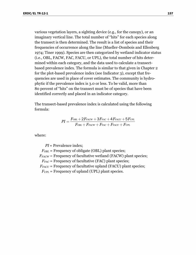
ERDC/EL TR-12-1 157
various vegetation layers, a sighting device (e.g., for the canopy), or an imaginary vertical line. The total number of “hits” for each species along the transect is then determined. The result is a list of species and their frequencies of occurrence along the line (Mueller-Dombois and Ellenberg 1974; Tiner 1999). Species are then categorized by wetland indicator status (i.e., OBL, FACW, FAC, FACU, or UPL), the total number of hits deter-mined within each category, and the data used to calculate a transect-based prevalence index. The formula is similar to that given in Chapter 2 for the plot-based prevalence index (see Indicator 3), except that fre-quencies are used in place of cover estimates. The community is hydro-phytic if the prevalence index is 3.0 or less. To be valid, more than 80 percent of “hits” on the transect must be of species that have been identified correctly and placed in an indicator category.
The transect-based prevalence index is calculated using the following formula:
OBL FACW FAC FACU UPL
OBL FACW FAC FACU UPL
F F F F FPI
F F F F F
2 3 4 5
where:
PI = Prevalence index; FOBL = Frequency of obligate (OBL) plant species; FFACW = Frequency of facultative wetland (FACW) plant species; FFAC = Frequency of facultative (FAC) plant species; FFACU = Frequency of facultative upland (FACU) plant species; FUPL = Frequency of upland (UPL) plant species.

ERDC/EL TR-12-1 158
Appendix C: Data Form
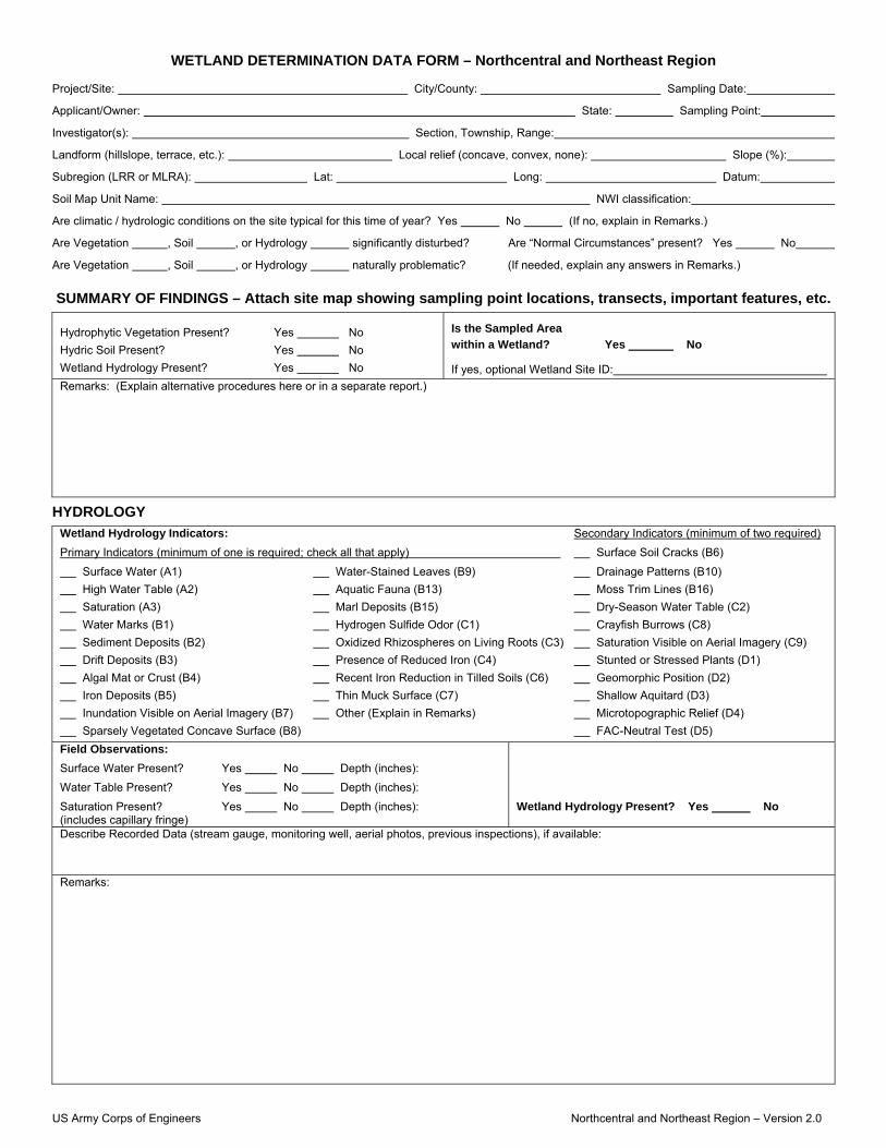
US Army Corps of Engineers Northcentral and Northeast Region – Version 2.0
WETLAND DETERMINATION DATA FORM – Northcentral and Northeast Region
Project/Site: City/County: Sampling Date:
Applicant/Owner: State: Sampling Point:
Investigator(s): Section, Township, Range:
Landform (hillslope, terrace, etc.): Local relief (concave, convex, none): Slope (%):
Subregion (LRR or MLRA): Lat: Long: Datum:
Soil Map Unit Name: NWI classification:
Are climatic / hydrologic conditions on the site typical for this time of year? Yes No (If no, explain in Remarks.)
Are Vegetation , Soil , or Hydrology significantly disturbed? Are “Normal Circumstances” present? Yes No
Are Vegetation , Soil , or Hydrology naturally problematic? (If needed, explain any answers in Remarks.)
SUMMARY OF FINDINGS – Attach site map showing sampling point locations, transects, important features, etc.
Hydrophytic Vegetation Present? Yes No
Hydric Soil Present? Yes No
Wetland Hydrology Present? Yes No
Is the Sampled Area
within a Wetland? Yes No
If yes, optional Wetland Site ID:
Remarks: (Explain alternative procedures here or in a separate report.)
HYDROLOGY
Wetland Hydrology Indicators: Secondary Indicators (minimum of two required)
Primary Indicators (minimum of one is required; check all that apply) Surface Soil Cracks (B6)
Surface Water (A1) Water-Stained Leaves (B9) Drainage Patterns (B10)
High Water Table (A2) Aquatic Fauna (B13) Moss Trim Lines (B16)
Saturation (A3) Marl Deposits (B15) Dry-Season Water Table (C2)
Water Marks (B1) Hydrogen Sulfide Odor (C1) Crayfish Burrows (C8)
Sediment Deposits (B2) Oxidized Rhizospheres on Living Roots (C3) Saturation Visible on Aerial Imagery (C9)
Drift Deposits (B3) Presence of Reduced Iron (C4) Stunted or Stressed Plants (D1)
Algal Mat or Crust (B4) Recent Iron Reduction in Tilled Soils (C6) Geomorphic Position (D2)
Iron Deposits (B5) Thin Muck Surface (C7) Shallow Aquitard (D3)
Inundation Visible on Aerial Imagery (B7) Other (Explain in Remarks) Microtopographic Relief (D4)
Sparsely Vegetated Concave Surface (B8) FAC-Neutral Test (D5)
Field Observations:
Surface Water Present? Yes No Depth (inches):
Water Table Present? Yes No Depth (inches):
Saturation Present? Yes No Depth (inches): (includes capillary fringe)
Wetland Hydrology Present? Yes No
Describe Recorded Data (stream gauge, monitoring well, aerial photos, previous inspections), if available:
Remarks:
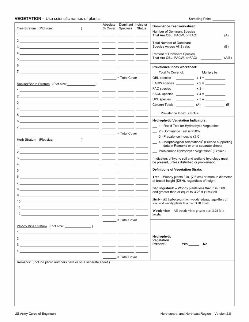
US Army Corps of Engineers Northcentral and Northeast Region – Version 2.0
VEGETATION – Use scientific names of plants. Sampling Point:
Absolute Dominant Indicator Tree Stratum (Plot size: ) % Cover Species? Status
1.
2.
3.
4.
5.
6.
7.
= Total Cover
Sapling/Shrub Stratum (Plot size: )
1.
2.
3.
4.
5.
6.
7.
= Total Cover
Herb Stratum (Plot size: )
1.
2.
3.
4.
5.
6.
7.
8.
9.
10.
11.
12.
= Total Cover
Woody Vine Stratum (Plot size: )
1.
2.
3.
4.
= Total Cover
Dominance Test worksheet:
Number of Dominant Species That Are OBL, FACW, or FAC: (A) Total Number of Dominant Species Across All Strata: (B) Percent of Dominant Species That Are OBL, FACW, or FAC: (A/B)
Prevalence Index worksheet:
Total % Cover of: Multiply by:
OBL species x 1 =
FACW species x 2 =
FAC species x 3 =
FACU species x 4 =
UPL species x 5 =
Column Totals: (A) (B)
Prevalence Index = B/A =
Hydrophytic Vegetation Indicators:
1 - Rapid Test for Hydrophytic Vegetation
2 - Dominance Test is >50%
3 - Prevalence Index is ≤3.01
4 - Morphological Adaptations1 (Provide supporting data in Remarks or on a separate sheet)
Problematic Hydrophytic Vegetation1 (Explain) 1Indicators of hydric soil and wetland hydrology must be present, unless disturbed or problematic.
Definitions of Vegetation Strata: Tree – Woody plants 3 in. (7.6 cm) or more in diameter at breast height (DBH), regardless of height. Sapling/shrub – Woody plants less than 3 in. DBH and greater than or equal to 3.28 ft (1 m) tall. Herb – All herbaceous (non-woody) plants, regardless of size, and woody plants less than 3.28 ft tall. Woody vines – All woody vines greater than 3.28 ft in height.
Hydrophytic Vegetation Present? Yes No
Remarks: (Include photo numbers here or on a separate sheet.)
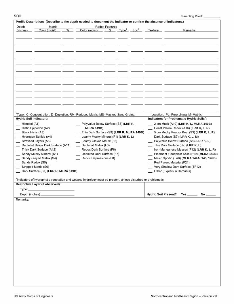
US Army Corps of Engineers Northcentral and Northeast Region – Version 2.0
SOIL Sampling Point:
Profile Description: (Describe to the depth needed to document the indicator or confirm the absence of indicators.)
Depth Matrix Redox Features (inches) Color (moist) % Color (moist) % Type1 Loc2 Texture Remarks
1Type: C=Concentration, D=Depletion, RM=Reduced Matrix, MS=Masked Sand Grains. 2Location: PL=Pore Lining, M=Matrix. Hydric Soil Indicators: Indicators for Problematic Hydric Soils3:
Histosol (A1) Polyvalue Below Surface (S8) (LRR R, 2 cm Muck (A10) (LRR K, L, MLRA 149B)
Histic Epipedon (A2) MLRA 149B) Coast Prairie Redox (A16) (LRR K, L, R)
Black Histic (A3) Thin Dark Surface (S9) (LRR R, MLRA 149B) 5 cm Mucky Peat or Peat (S3) (LRR K, L, R)
Hydrogen Sulfide (A4) Loamy Mucky Mineral (F1) (LRR K, L) Dark Surface (S7) (LRR K, L, M)
Stratified Layers (A5) Loamy Gleyed Matrix (F2) Polyvalue Below Surface (S8) (LRR K, L)
Depleted Below Dark Surface (A11) Depleted Matrix (F3) Thin Dark Surface (S9) (LRR K, L)
Thick Dark Surface (A12) Redox Dark Surface (F6) Iron-Manganese Masses (F12) (LRR K, L, R)
Sandy Mucky Mineral (S1) Depleted Dark Surface (F7) Piedmont Floodplain Soils (F19) (MLRA 149B)
Sandy Gleyed Matrix (S4) Redox Depressions (F8) Mesic Spodic (TA6) (MLRA 144A, 145, 149B)
Sandy Redox (S5) Red Parent Material (F21)
Stripped Matrix (S6) Very Shallow Dark Surface (TF12)
Dark Surface (S7) (LRR R, MLRA 149B) Other (Explain in Remarks)
3Indicators of hydrophytic vegetation and wetland hydrology must be present, unless disturbed or problematic.
Restrictive Layer (if observed):
Type:
Depth (inches):
Hydric Soil Present? Yes No Remarks:
REPORT DOCUMENTATION PAGE Form Approved
OMB No. 0704-0188 Public reporting burden for this collection of information is estimated to average 1 hour per response, including the time for reviewing instructions, searching existing data sources, gathering and maintaining the data needed, and completing and reviewing this collection of information. Send comments regarding this burden estimate or any other aspect of this collection of information, including suggestions for reducing this burden to Department of Defense, Washington Headquarters Services, Directorate for Information Operations and Reports (0704-0188), 1215 Jefferson Davis Highway, Suite 1204, Arlington, VA 22202-4302. Respondents should be aware that notwithstanding any other provision of law, no person shall be subject to any penalty for failing to comply with a collection of information if it does not display a currently valid OMB control number. PLEASE DO NOT RETURN YOUR FORM TO THE ABOVE ADDRESS.
1. REPORT DATE (DD-MM-YYYY) January 2012
2. REPORT TYPE Final report
3. DATES COVERED (From - To)
4. TITLE AND SUBTITLE
Regional Supplement to the Corps of Engineers Wetland Delineation Manual: Northcentral and Northeast Region (Version 2.0)
5a. CONTRACT NUMBER
5b. GRANT NUMBER
5c. PROGRAM ELEMENT NUMBER
6. AUTHOR(S)
U.S. Army Corps of Engineers
5d. PROJECT NUMBER
5e. TASK NUMBER
5f. WORK UNIT NUMBER
7. PERFORMING ORGANIZATION NAME(S) AND ADDRESS(ES) 8. PERFORMING ORGANIZATION REPORT
NUMBER U.S. Army Engineer Research and Development Center Environmental Laboratory 3909 Halls Ferry Road Vicksburg, MS 39180-6199
ERDC/EL TR-12-1
9. SPONSORING / MONITORING AGENCY NAME(S) AND ADDRESS(ES) 10. SPONSOR/MONITOR’S ACRONYM(S) Headquarters U.S. Army Corps of Engineers Washington, DC 20314-1000
11. SPONSOR/MONITOR’S REPORT NUMBER(S)
12. DISTRIBUTION / AVAILABILITY STATEMENT Approved for public release; distribution is unlimited.
13. SUPPLEMENTARY NOTES
14. ABSTRACT
This document is one of a series of Regional Supplements to the Corps of Engineers Wetland Delineation Manual, which provides technical guidance and procedures for identifying and delineating wetlands that may be subject to regulatory jurisdiction under Section 404 of the Clean Water Act or Section 10 of the Rivers and Harbors Act. The development of Regional Supplements is part of a nation-wide effort to address regional wetland characteristics and improve the accuracy and efficiency of wetland-delineation procedures. This supplement is applicable to the Northcentral and Northeast Region, which consists of all or portions of 15 states: Connecticut, Illinois, Indiana, Maine, Massachusetts, Michigan, Minnesota, New Hampshire, New Jersey, New York, Ohio, Pennsylvania, Rhode Island, Vermont, and Wisconsin.
15. SUBJECT TERMS Delineation Hydrology
Plant communities Soil
Vegetation Wetlands
16. SECURITY CLASSIFICATION OF: 17. LIMITATION OF ABSTRACT
18. NUMBER OF PAGES
19a. NAME OF RESPONSIBLE PERSON
a. REPORT
UNCLASSIFIED
b. ABSTRACT
UNCLASSIFIED
c. THIS PAGE
UNCLASSIFIED 175 19b. TELEPHONE NUMBER (include area code)
Standard Form 298 (Rev. 8-98)
Prescribed by ANSI Std. 239.18