Regional Patterns of Dead Wood in Forested Habitats of ... · USDA Forest Service Gen. Tech. Rep. PSW-GTR-181. 2002. 535 Regional Patterns of Dead Wood in Forested Habitats of Oregon

USDA Forest Service Gen. Tech. Rep. PSW-GTR-181. 2002. 535

Regional Patterns of Dead Wood in Forested Habitats of Oregon and Washington1

Janet L. Ohmann2 and Karen L. Waddell3

Abstract We describe regional patterns of variation in dead wood across 20 million ha of upland forests of all ownerships in Oregon and Washington, based on an analysis of data on snags and down wood collected on over 16,000 field plots. Current patterns of dead wood are highly variable and complex. The strongest differences were among nine habitats that reflect strong regional gradients in physical environment and ecosystem processes. Mean snag density was lowest in the drier habitats east of the Cascade crest and greatest at higher elevations, ranging from 0.8/ha to 37.2/ha. The mean volume of down wood ranged from 7.4 m3/ha in western juniper woodland to 183.3 m3/ha in westside conifer-hardwood forest. Differences in dead wood were more pronounced among habitats west of the Cascade crest. Dead wood abundance generally increased with successional development. Large snags were more than twice as dense within wilderness areas than outside wilderness, whereas large down wood was more abundant outside wilderness. Dead wood on plots was non-normally distributed and skewed to the right. Information on regional patterns of variation in dead wood is being incorporated into the DecAID model, which will help guide managers in considering dead wood and processes of decomposition in forest management. The regional summaries of dead wood also can be used to evaluate forest practice regulations and incentive programs for non-Federal lands, and to assess wildlife habitat suitability, ecosystem health, and carbon stores at state, regional, and national levels.

Introduction Dead trees are important elements of productive and biologically diverse forests.

Dead trees form major structural features with many ecological functions, including habitat for organisms, energy flow and nutrient cycling, and geomorphic processes (Harmon and others 1986). Yet, little is known about how amounts and characteristics of dead wood vary across broad regions that encompass a wide range of ecological conditions and disturbance histories.

Although the bulk of published data is from small-scale ecological plots, other forms of data exist but have not been analyzed. For example, resource inventories by Federal agencies include a wealth of information on snags (standing dead trees) and 1 An abbreviated version of this paper was presented at the Symposium on the Ecology and Management of Dead Wood in Western Forests, November 2-4, 1999, Reno, Nevada. 2 Research Forester, Pacific Northwest Research Station, USDA Forest Service, 3200 SW Jefferson Way, Corvallis, Oregon 97331 (e-mail: [email protected]) 3 Research Forester, Pacific Northwest Research Station, USDA Forest Service, P.O. Box 3890, Portland, Oregon, 97208 (e-mail: [email protected])

Dead Wood in Oregon and Washington Forests—Ohmann and Waddell


down wood (fallen trees) across the Pacific Northwest. This study describes current patterns of dead wood in Oregon and Washington by analyzing data collected on regional grids of field plots. In this paper we present a preliminary analysis of dead wood abundance in wildlife habitats of upland forests (“habitats”). We focused on 9 of the 31 major habitats that were developed for the Species Habitat Project (Chappell and others 2001). Our goal was to provide basic information about ecological patterns, as context for management decisions at stand, landscape, and ecoregion scales, and for analyzing forest policies at regional and national levels.

Study Area The study area encompasses a region of temperate forest within the states of

Washington and Oregon. The Cascade Range is the major topographic and climatic divide, and in this paper we refer to areas west of the Cascade crest as “westside” and east of the crest as “eastside.” Elevations range from sea level to nearly 3,000 m. Vulcanism shaped much of the landscape, but sedimentary and metamorphic rocks are plentiful, and deposition of parent materials by alluvial, colluvial, and eolian processes is common. Soil types are primarily inceptisols, spodosols, and ultisols. The westside has a maritime climate with wet winters and dry summers, and the eastside climate is drier and more continental.

Forests cover 19.6 million ha in the study area, about half of which is publicly owned (Powell and others 1993). Forests are dominated by coniferous trees (Franklin and Dyrness 1988). Hardwoods tend to occupy harsh sites, riparian areas, or disturbed areas, except in southwest Oregon. The mesic temperate coniferous forests of northwestern Washington and Oregon contain the greatest biomass accumulation and highest productivity rates in the world (Waring and Franklin 1979). See Franklin and Dyrness (1988) and Ohmann and Spies (1998) for detailed descriptions of Washington and Oregon plant communities and environmental gradients.

Before European settlement, fire was the predominant natural disturbance (Agee 1993), but in the last 100 years timber management and wildfire suppression have altered forest succession. Even-aged forest management practices are most common in northwestern Oregon and Washington, whereas uneven-aged management predominates in southwestern Oregon and on the eastside. On the eastside, fire suppression has allowed fire-sensitive and late-successional tree species to increase in density, and selective harvests have influenced forest composition.

Source of Data and Sample Design Data on dead wood have been collected from extensive grids of field plots as

part of ongoing, strategic-level inventories conducted by the USDA Forest Service in the Pacific Northwest for many years, and more recently by the USDI Bureau of Land Management (BLM) (table 1). National, state, and county parks and privately owned reserves had not been surveyed at the time of this study. Because plots were installed throughout the study area in a systematic fashion, the diversity of forests found in both states was sampled.



Table 1―Sources of data on live trees, snags, and down wood from regional forest inventories in Oregon and Washington.

Inventory program

Ownerships sampled

Sample grid spacing1

Sample weight2

Inventory dates

Number of plots3

Forest Inventory and Analysis (FIA)

Non-Federal 5.5 km 1.0 1984-1991 43,994

2.7 km outside

wilderness

0.25 1991-1995 11,958 Current Vegetation Survey (CVS)

National Forest

5.5 km inside

wilderness

1.0 1991-1995 580

Natural Resource Inventory (NRI)

Bureau of Land

Management in western

Oregon

5.5 km 1.0 1997 335

1 Plots on the 5.5-km grid represent about 3,000 ha; plots on the 2.7-km grid represent about 750 ha. 2 Weight applied to plot-level dead wood data in computing descriptive statistics. For NRI and CVS plots with multiple condition classes, weights were reduced proportional to the area occupied. 3 Includes only those plots on which dead wood data were collected. Does not include 319 plots in aspen, dunes, riparian, and wetland habitats. 4 Down wood data collected only on 886 plots in eastern Washington. Snag data collected on all plots.

The inventories provided data on stand characteristics, live trees, snags, and down wood collected on 16,867 field plots from 1984-1997 on forest land across Oregon and Washington (fig. 1). Field plots consisted of a cluster of up to five subplots and included a series of fixed- and variable-radius circular plots. The Forest Inventory and Analysis (FIA) plot was confined to a single, homogenous forest condition by moving subplots according to a predetermined pattern. In contrast, the Current Vegetation Survey (CVS) and Natural Resource Inventory (NRI) subplots were installed in fixed positions, and the plot could encompass multiple forest conditions. Live trees and snags were sampled on circular plots, and down wood was sampled along transect lines (DeVries 1973, Waddell 2002) established within plot boundaries. The species, diameter at breast height (DBH), and decay class (adapted from Cline and others 1980) were recorded for each snag tallied. Down wood measurements included the species, diameter at the point of intersection and at large end, piece length, decay class, and evidence of use by wildlife. Detailed information about inventory sample designs, field procedures, and compilation methods are available from the individual agencies that conducted the inventories (see also Max and others 1996, USDA Forest Service 1992, CVS Web site “www.fs.fed. us/r6/survey”).

We assigned each plot to an ecoregion (U.S. Environmental Protection Agency 1995) by overlaying the plot locations on the ecoregion map in a geographic information system (GIS). We also obtained data from the agencies on the reserve



status of each plot. Plots were coded as within areas set aside by Congress (Wilderness and Wild and Scenic Rivers), by agency administration or as unreserved.

Figure 1―Locations of Natural Resources Inventory (NRI), Current Vegetation Survey (CVS), and Forest Inventory and Analysis (FIA) field plots used in this study, Oregon and Washington. Only those plots where dead wood data were collected are shown. Black symbols are plots on Federal lands (NRI and CVS); gray symbols are plots on non-Federal lands (FIA).



Data Compilation and Analysis We compiled the source data from the three inventories into one database that

contains data tables for stand-level attributes, live trees, snags, and down wood. This involved converting codes and measurement units, calculating new variables, and making other technical modifications to insure that all data were in a common format for regional analysis. We calculated new variables from the down wood data collected with the line intersect sampling method to produce per-hectare estimates of down wood density (number of pieces), volume, and percent cover for each inventory plot (DeVries 1973, Waddell 2002). We also calculated per-hectare estimates of snag density. We were not able to compute snag volume at the time of this writing because many snag heights were missing in the CVS and NRI data.

We evaluated the CVS and NRI plots for the presence of multiple forest conditions. If a plot encompassed more than one land class (forest or nonforest), or more than one vegetation series (defined by the tree species that would dominate the site in the absence of disturbance) within forest land, we identified separate condition-classes on the plot. The live and dead tree data were partitioned among the condition-classes accordingly. We treated these condition-class plots as independent observations in our analyses, and refer to them simply as “plots” in this paper.

Stand-level variables and live tree data were used to classify each plot into a wildlife habitat type (“habitat”), alliance group, and successional stage. We used the habitats and some of the alliances from the classification system defined by the Species Habitat Project (Chappell and others 2001). We developed classification algorithms that utilized the set of variables we had available in the inventory database. Habitat was determined by evaluating the potential vegetation (series) and ecoregion assigned to the plot, and alliance was determined by examining a combination of potential and current vegetation variables as follows (scientific names of tree species are listed in appendix A): Habitat and alliance group Definition

Westside conifer-hardwood type: Western redcedar, Sitka spruce, western

hemlock, grand fir, white fir, and Port-Orford cedar series in westside ecoregions.

Hardwood alliance Hardwoods >70 pct and conifers <30 pct of stocking1

Conifer-hardwood mixed alliance Hardwoods 31-69 pct and conifers 31-69 pct of stocking1

Conifer alliance Hardwoods <30 pct and conifers >70 pct of stocking1; not a Sitka spruce site (see below).

Sitka spruce/western hemlock alliance Hardwoods <30 pct and conifers >70 pct of stocking1; Sitka spruce series or Sitka spruce present.

Westside white oak-Douglas-fir type: Douglas-fir or Oregon white oak series in westside ecoregions.

Douglas-fir alliance Douglas-fir series outside southwest Oregon; Oregon white oak absent.

Douglas-fir/white oak alliance Oregon white oak series or Oregon white oak present.

Southwest Oregon mixed conifer-hardwood type

Ponderosa pine, Douglas-fir, jeffrey pine, grand fir, white fir, Port-Orford cedar, tanoak, or canyon live oak series in southwest Oregon.



Habitat and alliance group

Definition

Montane mixed-conifer type Engelmann spruce, noble fir, Shasta red fir, Pacific silver fir, subalpine fir, and mountain hemlock series.

Subalpine parkland type Open parkland series of subalpine fir, mountain hemlock, subalpine larch, Alaska yellow-cedar, and whitebark pine.

Eastside mixed-conifer type Douglas-fir, grand fir, white fir, western redcedar, western hemlock, and noble fir series in eastside ecoregions.

Lodgepole pine type Lodgepole pine series in eastside ecoregions. Eastside ponderosa pine type: Ponderosa pine, Oregon white oak, and black

oak series in eastside ecoregions. Ponderosa pine/Douglas-fir alliance Oregon white and black oak absent. Ponderosa pine/white oak alliance Oregon white or black oak present. Western juniper type Western juniper series.

1 Relative stocking of all live trees in the stand, sensu Maclean (1979).

The Species Habitat Project (Chappell and others 2001) identified 26 structural stages of forest vegetation that are important as wildlife habitat. Because this classification system was too complex for our region-wide analysis, we grouped the 26 structural stages into three successional stages that we assume to be correlated with stand age or time since major disturbance. The stages were defined by current vegetation structure as follows: Successional Stage Definition

Early Tree stocking1 < 10 percent, or tree stocking >10 percent and quadratic mean diameter2 ranging from 2.5-24.9 cm.

Middle Tree stocking >10 percent and quadratic mean diameter2 ranging from 25.0-49.9 cm.

Late Tree stocking >10 percent and quadratic mean diameter2 > 50.0 cm.

___________________________________________________________________ 1 Relative stocking of all live trees in the stand on the plot, sensu Maclean (1979). 2 The diameter of the tree of average cross-sectional area at breast height (1.37 m) on the plot.

We computed descriptive statistics for snags and down wood within habitats by weighting the plots according to the sampling grid intensity (table 1) and the proportion of the plot within the condition-class. We summarized the characteristics of snags and down wood only for habitats and successional stages sampled by at least 10 plots. Wetlands, coastal dunes, aspen, and riparian forests were not well represented in the inventory sample and were excluded from our analysis.

We evaluated differences in dead wood among habitats using analysis of variance for unbalanced designs, with observations (plots) weighted as described above, using generalized linear models in SAS (SAS Institute Inc. 1988). We compared successional stages within each habitat and alliance and compared habitats with all successional stages combined. Where overall F tests were significant (alpha



> 0.05), we conducted multiple comparisons of means using the Tukey-Kramer method (SAS Institute Inc. 1988).

Because we used data collected from different sampling designs, a variety of tree tally criteria were applied in the field. Our snag and down wood analyses include trees of the following characteristics common to all datasets: snags >25.4 cm DBH and >2.0 m tall of decay classes 1-5; down wood >12.5 cm diameter at point of intersection and >2.0 m long of decay classes 1-5 (except decay classes 1-4 for FIA plots). We summarize dead wood for two groups: “total snags” or “total down wood,” which includes snags >25.4 cm DBH or down wood > 12.5 cm diameter at large end; and “large snags” or “large down wood,” which includes snags >50 cm DBH or down wood > 50 cm diameter at large end.

Results Differences in Dead Wood Among Habitats and Alliances

We present snag results in terms of density (tables 2-3), and down wood in terms of volume (tables 4-5), cover (tables 6-7), and density (tables 8-9). We limit our discussion of down wood to volume, but patterns of cover and density were similar. All results represent weighted means of plot-level, per-hectare estimates for a category of interest.

The abundance of snags and down wood varied substantially across the region. The greatest differences in dead wood were among the habitats, although differences among successional stages within habitats also were significant in many cases. Total snag densities were greatest at higher elevations: 37.2/ha in montane mixed-conifer forest and 36.0/ha in subalpine parks (table 2). Snags were least dense in the drier habitats on the eastside: 0.8/ha in western juniper woodland and 5.0/ha in eastside ponderosa pine (table 2). Large snags were most abundant in montane mixed-conifer forest (9.6/ha) and in westside conifer-hardwood forest (5.5/ha), and least abundant in western juniper woodland (0.2/ha) and eastside ponderosa pine woodland (1.0/ha) (table 3). The volumes of both total and large down wood were greatest in westside conifer-hardwood forest and lowest in western juniper woodland (table 4). Total down wood volume among habitats ranged from 7.4 to 183.3 m3/ha and large wood from 4.5 to 131.8 m3/ha.

Pairwise differences in total dead wood generally were more pronounced among habitats west of the Cascades than among the eastside types. Differences between westside habitats (conifer-hardwood, white oak-Douglas-fir, southwest Oregon mixed conifer-hardwood) were always significant for both snags and down wood. The amounts of total snags and down wood in montane mixed-conifer forests were significantly different from almost all other habitats.

Successional Patterns of Dead Wood Snag density generally increased with stand development. Within habitats and

alliances, total snag density always was lowest in the early successional stage and usually was highest in the late stage (table 2). The abundance of large snags increased with successional development in all of the habitats and alliances except the hardwood alliance of westside conifer-hardwood forest and in western juniper woodland, where differences were not significant (table 3). Differences in snag



density were significant between at least two successional stages in all of the habitats and alliances except the hardwood alliance of westside conifer-hardwood forest, the eastside ponderosa pine alliances, and western juniper woodland (tables 2-3).

The volume of down wood also generally increased with forest development, but successional patterns differed somewhat among the habitats and alliances (tables 4-5). Late successional stages contained the largest concentrations of both total and large down wood in most of the habitats and alliances (tables 4-5). In the westside habitats and in montane mixed-conifer forest, down wood volume in the late stage usually was significantly different from the early and middle stages, but early and middle stages usually were not significantly different from one another (tables 4-5). Large down wood volumes differed significantly between the early and middle successional stages in all of the eastside habitats and alliances except the ponderosa pine/white oak alliance and western juniper woodland (table 5). Table 2―Weighted mean (standard error) density of “total” snags >25.4 cm DBH, decay classes 1-5, and >2 m tall by habitat, alliance, and successional stage, Oregon and Washington.1

Successional stage

Habitat and alliance Early Middle Late All stages

Mean (SE) trees per hectare Westside conifer-hardwood: Hardwood 5.6 (1.1) 13.3 (1.2) 9.3 (3.6) 11.0 (0.9) Conifer-hardwood mixed a5.3 (0.8) b12.3 (0.9) b14.6 (1.9) 10.2 (0.6) Conifer a5.2 (0.4) b21.4 (0.8) c34.0 (1.1) 16.1 (0.5) Sitka spruce/western hemlock

a4.3 (0.7) b16.1 (1.4) b27.8 (3.1) 12.4 (0.9)

All alliances a5.1 (0.3) b17.9 (0.6) c31.4 (1.0) 14.3 (0.3) Westside white oak-Douglas-fir: Douglas-fir 6.5 (2.3) 12.2 (2.0) 20.7 (4.0) 11.6 (1.5) Douglas-fir/white oak a6.1 (1.3) a10.6 (1.3) b14.5 (3.0) 9.3 (0.9) All alliances a6.3 (1.1) a11.3 (1.1) b17.1 (2.5) 10.2 (0.8) Southwest Oregon mixed conifer-hardwood

a9.5 (1.1) b17.1 (0.9) b21.0 (1.0) 15.4 (0.6)

Montane mixed-conifer a17.8 (1.4) b49.3 (1.3) c40.3 (1.4) 37.2 (0.9) Subalpine parkland 34.8 (7.4) 37.3 (4.3) 2 NA 36.0 (4.3) Eastside mixed-conifer a14.8 (0.9) b21.5 (0.6) 20.7 (1.6) 19.4 (0.5) Lodgepole pine a16.5 (1.5) b27.6 (2.6) 2 NA 19.8 (1.3) Eastside ponderosa pine: Ponderosa pine/Douglas-fir 4.8 (0.5) 4.8 (0.4) 5.3 (0.8) 4.8 (0.3) Ponderosa pine/white oak 7.1 (1.6) 7.5 (1.9) 2 NA 7.1 (1.2) All alliances 5.0 (0.4) 5.0 (0.4) 5.2 (0.8) 5.0 (0.3) Western juniper 0.7 (0.2) 1.6 (0.4) 0.8 (0.5) 0.8 (0.2) All habitats a9.1 (0.3) b21.3 (0.3) c28.4 (0.6) 17.4 (0.2)

1 Significantly different means (alpha < 0.05) within rows (among successional stages) are indicated by different letter footnotes. 2 Not applicable—sample size <10 plots.



Table 3―Weighted mean (standard error) density of “large” snags >50.0 cm DBH, decay classes 1-5, and >2 m tall by habitat, alliance, and successional stage, Oregon and Washington.1 Successional stage


Mean (SE) trees per hectare Westside conifer-hardwood: Hardwood 2.6 (0.6) 3.5 (0.4) 2.0 (1.0) 3.2 (0.3) Conifer-hardwood mixed a2.1 (0.5) b4.2 (0.3) b7.8 (1.1) 3.7 (0.3) Conifer a2.1 (0.2) b7.5 (0.4) c15.6 (0.5) 6.4 (0.2) Sitka spruce/western hemlock

a2.1 (0.3) b5.3 (0.5) c12.4 (1.4) 4.7 (0.3)

All alliances a2.1 (0.1) b6.0 (0.2) c14.3 (0.5) 5.5 (0.2) Westside white oak- Douglas-fir:

Douglas-fir 2.5 (1.1) 3.3 (0.5) 7.6 (1.4) 3.5 (0.5) Douglas-fir/white oak a0.9 (0.2) b2.0 (0.3) c4.8 (1.0) 1.9 (0.2) All alliances a1.4 (0.4) a2.6 (0.3) b5.9 (0.9) 2.5 (0.2) Southwest Oregon mixed conifer-hardwood

a2.6 (0.3) b5.0 (0.3) c9.5 (0.5) 5.1 (0.2)

Montane mixed-conifer a3.0 (0.3) b10.5 (0.4) c21.7 (0.7) 9.6 (0.3) Subalpine parkland a1.7 (0.5) b5.6 (1.0) 2 NA 3.6 (0.6) Eastside mixed-conifer a2.1 (0.2) b4.2 (0.1) c8.0 (0.6) 3.8 (0.1) Lodgepole pine a0.8 (0.1) b2.2 (0.3) 2 NA 1.2 (0.1) Eastside ponderosa pine: Ponderosa pine/Douglas-fir 0.9 (0.1) 0.9 (0.1) 1.4 (0.3) 0.9 (0.1) Ponderosa pine/white oak 1.0 (0.4) 3.2 (1.0) 2 NA 2.1 (0.6) All alliances 0.9 (0.1) 1.1 (0.1) 1.4 (0.2) 1.0 (0.1) Western juniper 0.1 (0.0) 0.5 (0.2) 0.1 (0.2) 0.2 (0.1) All habitats a2.0 (0.1) b5.3 (0.1) c13.3 (0.3) 4.9 (0.1)

1Significantly different means (alpha < 0.05) within rows (among successional stages) are indicated by different letter footnotes. 2 Not applicable—sample size <10 plots.



Table 4―Weighted mean (standard error) volume of “total” down wood >12.5 cm large end diameter, decay classes 1-4, and >2.0 m long by habitat, alliance, and successional stage, Oregon and Washington.1

Successional stage


Mean (SE) cubic meters per hectare Westside conifer-hardwood: Hardwood 67.0 (20.1) 142.0 (33.1) 2 NA 125.0 (23.7) Conifer-hardwood mixed 192.1 (31.6) 166.6 (24.7) 148.3 (39.1) 172.2 (17.4) Conifer a150.8 (8.2) a168.4 (6.7) b229.2 (9.0) 185.4 (4.7) Sitka spruce/western hemlock

a123.6 (27.2) 173.2 (22.2) b232.2 (29.8) 183.4 (15.8)

All alliances a151.8 (7.6) a167.7 (6.2) b226.3 (8.4) 183.3 (4.3) Westside white oak- Douglas-fir:

Douglas-fir 82.8 (18.6) 57.7 (13.5) 88.8 (20.6) 70.7 (9.6) Douglas-fir/white oak 26.4 (10.7) 36.3 (4.2) 57.0 (12.0) 37.8 (4.0) All alliances 54.0 (11.7) 44.2 (6.1) 71.2 (12.3) 51.3 (5.1) Southwest Oregon mixed conifer-hardwood

a84.9 (8.6) a68.8 (4.6) b118.6 (8.0) 85.9 (3.8)

Montane mixed-conifer a102.1 (6.4) a112.5 (3.3) b198.5 (10.6) 123.8 (3.2) Subalpine parkland 35.1 (7.3) 55.2 (10.4) 2 NA 44.0 (6.3) Eastside mixed-conifer a47.0 (2.2) b54.6 (1.3) b58.8 (4.9) 52.7 (1.1) Lodgepole pine 50.0 (2.5) 55.4 (4.2) 2 NA 51.4 (2.2) Eastside ponderosa pine: Ponderosa pine/Douglas-fir a21.6 (1.4) b27.8 (1.4) 20.2 (3.0) 25.1 (1.0) Ponderosa pine/white oak 16.9 (6.7) 35.5 (9.7) 2 NA 27.4 (6.3) All alliances a21.3 (1.3) b28.4 (1.4) 19.7 (3.0) 25.3 (1.0) Western juniper 7.5 (3.1) 7.3 (1.9) 7.5 (4.7) 7.4 (1.9) All habitats a70.0 (1.9) b77.6 (1.3) c161.4 (4.5) 87.8 (1.2)




Table 5―Weighted mean (standard error) volume of “large” down wood >50.0 cm large end diameter, decay classes 1-4, and >2.0 m long by habitat, alliance, and successional stage, Oregon and Washington.1

Successional stage


Mean (SE) cubic meters per hectare Westside conifer-hardwood: Hardwood 43.8 (17.8) 109.1 (32.7) 2 NA 95.5 (23.2) Conifer-hardwood mixed 146.9 (29.3) 129.0 (23.0) 112.4 (39.2) 132.3 (16.4) Conifer a95.4 (7.3) a118.6 (6.3) b173.9 (8.5) 132.3 (4.4) Sitka spruce/western hemlock

a79.6 (25.7) 129.1 (21.6) b180.8 (27.4) 136.6 (14.9)

All alliances a98.5 (6.8) a119.6 (5.7) b172.1 (8.0) 131.8 (4.0) Westside white oak-Douglas-fir:


a53.6 (7.5) a42.6 (4.0) b83.8 (7.4) 56.2 (3.4)

Montane mixed-conifer a48.9 (5.6) a46.2 (2.4) b144.9 (9.6) 63.4 (2.8) Subalpine parkland 7.3 (3.3) 22.3 (6.4) 2 NA 14.5 (3.8) Eastside mixed-conifer a17.3 (1.8) b23.0 (1.0) c35.9 (4.2) 22.2 (0.9) Lodgepole pine a5.6 (0.9) b14.6 (2.8) 2 NA 8.1 (1.0) Eastside ponderosa pine: Ponderosa pine/Douglas- fir

a10.4 (1.1) b15.1 (1.2) 11.6 (2.4) 13.2 (0.8)

Ponderosa pine/white oak

8.7 (5.3) 20.3 (7.6) 2 NA 15.2 (4.9)

All alliances a10.3 (1.1) b15.5 (1.2) 11.2 (2.4) 13.4 (0.8) Western juniper 5.0 (2.8) 3.5 (1.6) 6.2 (4.6) 4.5 (1.7) All habitats a34.7 (1.6) b40.5 (1.1) c118.6 (4.1) 50.4 (1.0)




Table 6―Weighted mean (standard error) percent cover of “total” down wood >12.5 cm large end diameter, decay classes 1-4, and >2.0 m long by habitat, alliance, and successional stage, Oregon and Washington.1 Successional stage


Mean (SE) percent cover Westside conifer-hardwood: Hardwood 2.1 (0.5) 3.4 (0.5) 2 NA 3.1 (0.4) Conifer-hardwood mixed 4.4 (0.6) 4.1 (0.5) 3.5 (0.6) 4.1 (0.3) Conifer a4.5 (0.2) a4.6 (0.1) b5.6 (0.2) 4.9 (0.1) Sitka spruce/western hemlock a3.5 (0.5) 4.7 (0.4) b5.6 (0.6) 4.8 (0.3) All alliances a4.4 (0.2) a4.5 (0.1) b5.5 (0.2) 4.8 (0.1) Westside white oak-Douglas-fir: Douglas-fir 2.7 (0.4) 1.7 (0.3) 2.6 (0.5) 2.2 (0.2) Douglas-fir/white oak a1.0 (0.3) 1.4 (0.1) b1.8 (0.3) 1.4 (0.1) All alliances 1.8 (0.3) 1.5 (0.1) 2.2 (0.3) 1.7 (0.1) Southwest Oregon mixed conifer-hardwood

a2.5 (0.2) a2.2 (0.1) b3.2 (0.2) 2.5 (0.1)

Montane mixed-conifer a3.8 (0.2) b4.3 (0.1) c5.1 (0.2) 4.3 (0.1) Subalpine parkland 1.6 (0.3) 2.1 (0.4) 2 NA 1.8 (0.2) Eastside mixed-conifer 2.0 (0.1) a2.2 (0.0) b1.9 (0.1) 2.1 (0.0) Lodgepole pine 2.9 (0.1) 2.8 (0.2) 2 NA 2.9 (0.1) Eastside ponderosa pine: Ponderosa pine/Douglas-fir a0.9 (0.0) b1.0 (0.0) a0.7 (0.1) 0.9 (0.0) Ponderosa pine/white oak 0.7 (0.2) 1.2 (0.3) 2 NA 1.0 (0.2) All alliances a0.8 (0.0) b1.0 (0.0) a0.7 (0.1) 0.9 (0.0) Western juniper 0.2 (0.1) 0.3 (0.1) 0.3 (0.2) 0.2 (0.0) All habitats a2.6 (0.1) b2.7 (0.0) c4.1 (0.1) 2.9 (0.0)




Table 7―Weighted mean (standard error) percent cover of “large” down wood >50.0 cm large end diameter, decay classes 1-4, and >2.0 m long by habitat, alliance, and successional stage, Oregon and Washington.

Successional stage


Mean (SE) percent cover Westside conifer-hardwood: Hardwood 0.9 (0.3) 1.8 (0.5) 2 NA 1.7 (0.4) Conifer-hardwood mixed 2.5 (0.4) 2.2 (0.4) 1.8 (0.5) 2.2 (0.3) Conifer alliance a1.8 (0.1) a2.2 (0.1) b3.1 (0.1) 2.4 (0.1) Sitka spruce/western hemlock a1.3 (0.3) 2.6 (0.4) b3.2 (0.4) 2.5 (0.2) All alliances a1.9 (0.1) a2.2 (0.1) b3.1 (0.1) 2.4 (0.1) Westside white oak-Douglas-fir: Douglas-fir 0.9 (0.3) 0.8 (0.2) 0.9 (0.3) 0.8 (0.1) Douglas-fir/white oak 0.3 (0.2) 0.5 (0.1) 0.8 (0.2) 0.5 (0.1) All alliances 0.6 (0.2) 0.6 (0.1) 0.9 (0.2) 0.6 (0.1) Southwest Oregon mixed conifer-hardwood

a0.9 (0.1) a0.9 (0.1) b1.6 (0.1) 1.1 (0.1)

Montane mixed-conifer a1.0 (0.1) a1.0 (0.0) b2.9 (0.2) 1.3 (0.1) Subalpine parkland 0.2 (0.1) 0.5 (0.1) 2 NA 0.4 (0.1) Eastside mixed-conifer a0.4 (0.0) b0.5 (0.0) c0.7 (0.1) 0.5 (0.0) Lodgepole pine a0.2 (0.0) b0.3 (0.1) 2 NA 0.2 (0.0) Eastside ponderosa pine: Ponderosa pine/Douglas-fir a0.2 (0.0) b0.3 (0.0) 0.3 (0.1) 0.3 (0.0) Ponderosa pine/white oak 0.2 (0.1) 0.4 (0.2) 2 NA 0.3 (0.1) All alliances a0.2 (0.0) b0.3 (0.0) 0.3 (0.1) 0.3 (0.0) Western juniper 0.1 (0.0) 0.1 (0.0) 0.2 (0.2) 0.1 (0.0) All habitats a0.7 (0.0) b0.8 (0.0) c2.2 (0.1) 1.0 (0.0)




Table 8―Weighted mean (standard error) density of “total” down wood >12.5 cm large end diameter, decay classes 1-4, and >2.0 m long by habitat, alliance, and successional stage, Oregon and Washington. Successional stage


Mean (SE) pieces per hectare Westside conifer-hardwood: Hardwood 199.4 (43.2) 193.0 (36.3) 2 NA 185.9 (26.5) Conifer-hardwood mixed 277.5 (39.0) 234.6 (22.2) 152.2 (29.5) 233.5 (18.1) Conifer a338.6 (15.7) a255.4 (7.5) b252.9 (7.2) 274.5 (5.5) Sitka spruce/western hemlock

a244.8 (40.4) 281.4 (24.3) b276.2 (34.4) 271.3 (18.5)

All alliances a326.5 (13.9) a254.3 (6.8) b250.8 (7.0) 271.0 (5.1) Westside white oak-Douglas-fir: Douglas-fir 220.8 (34.4) 104.8 (15.9) 140.1 (25.6) 136.7 (13.6) Douglas-fir/white oak a87.9 (37.9) 97.1 (11.4) b107.0 (19.7) 97.6 (10.4) All alliances 174.1 (27.4) 101.5 (10.2) 128.2 (18.5) 120.8 (9.3) Southwest Oregon mixed conifer-hardwood

a158.9 (14.5) a147.4 (7.8) b172.3 (9.4) 157.0 (5.7)

Montane mixed-conifer a254.1 (10.1) b250.3 (6.5) c222.3 (9.3) 246.7 (4.8) Subalpine parkland 113.1 (17.2) 129.0 (19.4) 2 NA 118.2 (12.5) Eastside mixed-conifer 158.0 (4.9) a142.9 (2.7) b102.2 (6.6) 144.5 (2.3) Lodgepole pine 201.6 (8.5) 161.2 (12.3) 2 NA 190.9 (7.0) Eastside ponderosa pine: Ponderosa pine/Douglas-fir a71.1 (4.0) b77.5 (3.0) a43.7 (6.9) 73.0 (2.3) Ponderosa pine/white oak 57.4 (23.9) 94.4 (16.9) 2 NA 80.2 (13.5) All alliances a70.1 (3.9) b78.8 (3.0) a44.8 (6.8) 73.5 (2.3) Western juniper 16.4 (4.3) 23.1 (6.1) 26.9 (16.4) 19.2 (3.4) All habitats a182.9 (3.5) b167.2 (2.1) c191.4 (4.0) 175.5 (1.7)




Table 9―Weighted mean (standard error) density of “large” down wood >50.0 cm large end diameter, decay classes 1-4, and >2.0 m long by habitat, alliance, and successional stage, Oregon and Washington.

Successional stage


Mean (SE) pieces per hectare Westside conifer-hardwood: Hardwood 33.4 (12.6) 52.8 (17.1) 2 NA 45.7 (11.1) Conifer-hardwood mixed 71.8 (11.2) 48.1 (9.9) 32.2 (7.6) 53.4 (6.1) Conifer a60.0 (4.5) a47.4 (2.5) b59.7 (2.8) 54.8 (1.8) Sitka spruce/western hemlock

a32.3 (9.4) 67.9 (11.5) b72.7 (11.9) 62.0 (6.8)

All alliances a59.0 (4.0) a48.7 (2.3) b59.6 (2.7) 55.0 (1.7) Westside white oak- Douglas-fir:


a19.6 (2.9) a18.3 (2.1) b29.6 (3.0) 21.9 (1.5)

Montane mixed-conifer a25.4 (2.3) a21.5 (1.1) b57.8 (3.6) 28.6 (1.1) Subalpine parkland 6.5 (3.0) 10.9 (3.4) 2 NA 8.5 (2.2) Eastside mixed-conifer a8.9 (0.6) b10.5 (0.4) c15.7 (1.7) 10.4 (0.3) Lodgepole pine a4.2 (0.7) b7.9 (1.7) 2 NA 5.3 (0.7) Eastside ponderosa pine: Ponderosa pine/Douglas-fir a5.8 (0.6) b7.1 (0.6) 6.4 (1.5) 6.6 (0.4) Ponderosa pine/white oak 6.3 (5.5) 8.8 (3.0) 2 NA 7.6 (2.7) All alliances a5.8 (0.6) b7.2 (0.5) 6.2 (1.4) 6.6 (0.4) Western juniper 1.0 (0.5) 1.9 (1.0) 11.0 (8.2) 1.8 (0.6) All habitats a17.5 (0.8) b17.1 (0.4) c43.2 (1.4) 21.0 (0.4)




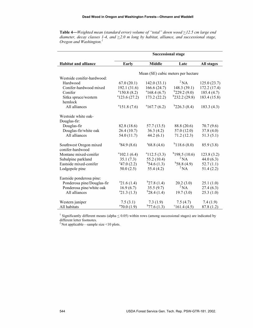
Dead Wood in Wilderness Areas Our analysis indicated that over all habitats, large snags were more than twice as

dense in Federal wilderness areas than outside wilderness (fig. 2A). The strongest differences were for westside conifer-hardwood forest (5.1/ha outside wilderness vs. 15.2/ha inside wilderness), eastside mixed-conifer forest (3.2/ha vs. 9.5/ha), and lodgepole pine (0.8/ha vs. 3.4/ha). In contrast, large down wood was more abundant outside wilderness areas than in wilderness in all of the habitats (fig. 2B), although the differences often were not significant. The most pronounced differences in down wood volume were for southwest Oregon mixed conifer-hardwood (64.3 m3/ha outside wilderness vs. 22.6 m3/ha inside wilderness) and montane mixed-conifer (74.3 m3/ha vs. 35.2 m3/ha).

About 6.5 percent of the total area sampled for dead wood was in federally designated wilderness areas. The higher elevation habitats were best represented: 57 percent of the sampled area in subalpine park and 32 percent of montane mixed-conifer forest was in wilderness. Most poorly represented were western juniper woodland, eastside ponderosa pine, and westside conifer-hardwood forest (1.0, 0.3, and 1.5 percent of the sampled area, respectively).

Discussion Causes of Regional Variability in Dead Wood Abundance

The regional differences in dead wood abundance among wildlife habitats reflect strong underlying gradients in physical environment and biological processes that affect community composition and structure, forest dynamics, and rates of dead wood input and decomposition. The amount and characteristics of dead wood in an ecosystem represent a balance between additions through tree death, breakage, and transport, and losses through processes of decomposition and fire consumption (Harmon and others 1986). The factors that influence these processes, and thus the spatial and temporal patterns of dead wood, are scale-dependent and incredibly complex. Our intent in this analysis was to present preliminary regional summaries of dead wood within vegetation types that describe distinct wildlife habitats in upland forests. (An in-depth analysis of factors that explain these patterns is beyond the scope of this paper.)

Westside conifer-hardwood forests have the highest net primary productivity of the habitats (Franklin 1988). Forest stands with greater density of live trees can be expected to have greater amounts of dead trees as well, and the high amount of dead wood we observed in the westside conifer-hardwood habitat probably can be explained by high rates of input within these productive forests. Rates of dead wood input also are influenced by rates of live tree mortality, which can increase as tree density surpasses that of a fully stocked stand. The large amount of dead wood in montane mixed-conifer forest may be explained in part by slow rates of decomposition in the cold temperatures at high elevations. The higher density of snags in the subalpine parkland and montane mixed-conifer types may be attributed to high mortality and low fall rates in these wildlife habitats. Unfortunately, published information on regional variation in rates of mortality, dead wood input, and decomposition, which would be very useful in interpreting our regional patterns of dead wood abundance, is scanty. A summary of existing studies in Washington and Oregon (Harmon and others 1986) showed greater input rates of dead wood



biomass in mature and old-growth Douglas-fir and Sitka spruce/western hemlock forests (0.5-30 mg/ha/yr) than in higher elevation Pacific silver fir (0.3 mg/ha/yr), but data were not available for eastside forests.

Figure 2―Abundance of dead wood by habitat and wilderness status, Oregon and Washington: A) is the weighted mean density of snags >50.0 cm DBH, decay classes 1-5, and >2 m tall; B) is the weighted mean volume of down wood >50.0 cm diameter at the large end, decay classes 1-4, and >2 m long. Error bars indicate one standard error of the mean. WCNH = westside conifer-hardwood, WODF = white oak-Douglas-fir, SWOMCH = southwest Oregon mixed conifer-hardwood, MMC = montane mixed-conifer, PARK = subalpine parkland, EMC = eastside mixed-conifer, LP = lodgepole pine, EPPWO = eastside ponderosa pine-white oak, JUN = western juniper, ALL = all wildlife habitats. There were <10 plots in western juniper in wilderness.

(a) Snags >=50 cm DBH

02468

1012141618

WCN

H

WO

DFSW

OM

CH

MM

C

PARK

EMC LP

EPPW

O

JUN

ALL

Mea

n tre

es p

er h

a

Outside wildernessIn wilderness

(b) Down wood >=50 cm diameter at the large end

0

20

406080

100

120

140160

WCN

H

WO

DFSW

OM

CH

MM

C

PARK

EMC LP

EPPW

O

JUN

ALL

Mea

n cu

bic

met

ers

per h

a

Outside wildernessIn wilderness

A)

B)



Current dead wood on a site also is influenced by disturbance and development of the current stand, and by the amounts of wood inherited from the preceding stand. Unfortunately, consistent information on the history of natural and human disturbance to the plots was not available for our analysis. Nevertheless, the successional stages used in our study represent distinct structural conditions that are surrogates for a chronosequence of stand development after stand-replacing disturbance. Although rate of biomass input and average piece size generally are thought to increase with succession (Harmon and others 1986), the amount of dead wood can follow a U-shaped pattern if young forests inherit large amounts of dead wood and live trees from preceding stands (Spies and others 1988). The snags in our study—especially large snags—increased with succession in almost all of the habitats. No wildlife habitats exhibited a U-shaped pattern, probably because snags tend to be cut within harvest units, which reduces the density found in early successional forests. Down wood also most often increased with succession, but this pattern was less consistent than for snags, and some habitats did exhibit a U-shaped pattern. Because we lacked data on the disturbance history of the plots and on the origin of individual pieces (from the current or a preceding stand), we can only speculate on why the habitats differed in this regard.

The lack of a U-shaped successional pattern for snags is not surprising. Snags have much shorter lag times in the forest than down wood: natural processes of fragmentation and decomposition begin much sooner, and they disappear as recognizable structures much faster (Harmon and others 1986). In addition, much of the dead wood in westside forests is input directly as down wood rather than snags (Harmon and others 1986). Snags also are much more likely than down wood to be damaged or intentionally removed by humans through the course of forest management and harvest activities. In an analysis of a subset of the same FIA data we used in this study (40- to 200-year-old stands on non-Federal lands in northwestern Oregon), Hansen and others (1991) found that large snags (>50.8 cm DBH) were three to five times as dense in stands that had never been clearcut than in stands that had been clearcut at least once. These factors taken together suggest that snag levels would more closely track recent disturbance and forest succession, while down wood amounts would be more strongly influenced by the long-term history and productivity of the site.

Information on the reserve status of the plots was our only available means for identifying forests unlikely to have been disturbed by timber harvesting and management. However, our comparisons of dead wood within and outside of wilderness areas must be interpreted with caution. Perhaps most importantly, the plots in wilderness do not sample complete environmental gradients—they are strongly biased towards higher elevations and lower productivities. We suspect these inherent productivity differences explain much of the higher amounts of down wood outside wilderness. On the other hand, if snags are more strongly influenced (i.e., reduced) by timber management activities than down wood as we suspect, then wilderness areas would be more likely to contain greater amounts of snags than areas outside wilderness—which is indeed what our data showed. In fact, Occupational Health and Safety Administration (OSHA) standards require the removal of most snags from harvest units for worker safety. Therefore, we would expect to find fewer snags in managed stands outside wilderness. If snags are cut and left on site, this would contribute to the larger amount of down wood we observed outside wilderness areas. In addition, high snag densities in higher elevation wildlife habitats (subalpine parkland and montane mixed conifer) could be the result of these areas being less



accessible and less likely to be harvested for timber or firewood, regardless of their reserve status. Although wilderness areas are off-limits to future timber harvesting, they have been affected by other human activities to some degree (e.g., fire suppression, roads, recreation, exotic species introduction). Furthermore, many plots outside wilderness areas sample old-growth and younger forest on sites that have never been harvested.

Comparisons with Other Studies Very few estimates of dead wood abundance at broad geographic scales are

available for comparison with our numbers. Indeed, the lack of this kind of information was the primary motivation for this study. Direct comparisons are extremely difficult to make because of differences among studies in geographic location; the vegetation types, stand ages, and disturbance histories sampled; sampling design; definitions (e.g., dead wood sizes and decay classes); and units of measure (numbers of trees, volume, density, cover, or linear meters). Furthermore, this information often is not provided in the publications. Other regional studies of dead wood in Washington and Oregon have been restricted either to Federal or to nonfederal lands, which usually represent very different ecological conditions (Ohmann and Spies 1998). The study by Ohmann and others (1994) was limited to snags on non-Federal lands (a subset of the FIA data used in this paper), because data were unavailable for dead wood on Federal lands and down wood on non-Federal lands at that time. The study by Spies and others (1988) was confined to natural Douglas-fir forests > 40 years old on Federal lands on the westside. Published information for eastside forests is not available (Everett and others 1999), or consists of summaries of a few local studies (Bull and others 1997). Scientists for the Interior Columbia River Basin Ecosystem Management Project relied on expert opinion and local studies to estimate current and historical amounts of dead wood (Korol and others 2002). Harmon and others (1986) did not include any studies from eastern Washington or eastern Oregon.

Our large snag densities in westside conifer-hardwood forest (table 3) were substantially less than those reported by Spies and others (1988): our estimate of 2.1 large snags/ha in early stages probably represent stands younger than the 40 yr minimum sampled by Spies and others (1988); our estimate for middle-successinal stages of 6.0/ha compares to 27/ha in their young stands; and our estimate for late stages of 14.3/ha compares to their mature (16/ha) and old-growth (27/ha) classes.

On first inspection our estimates of down wood volume appear somewhat lower than other published numbers, but direct comparisons are not possible for reasons cited above. Although our estimates of mean down wood volume in successional stages of westside conifer-hardwood forest ranged from 151.8 to 226.3 m3/ha (table 4), our maximum value on a plot was 2,142.9 m3/ha. This compares to a range of 309 to 1,421 m3/ha in various studies in westside Douglas-fir-western hemlock summarized by Harmon and others (1986) (table 4), and to 148 to 313 m3/ha reported by Spies and others (1988).

We expect our estimates of down wood to be lower than other published studies for several reasons: our minimum diameter of 12.5 cm was slightly larger than the 10 cm minimum found in many other studies, which would reduce the number of down logs in the sample; we included managed as well as natural forests of all ages, not just older natural forests originating after fire; we excluded down wood of decay



class 5; and our numbers are means across many stands, including stands where no down wood was observed (e.g., zero-tally plots), and maximum values are not presented. Our estimates of percent cover of down wood also may be lower than in other studies that used plot sampling or total tallies, as percent cover calculated from line intersect sampling has been shown to underestimate true values (Bate and others 1999).

Our dead wood estimates are not directly comparable to those reported in most wildlife studies (Marcot and others 2002). These studies typically are conducted within a local area and describe dead wood around nest sites, where it may be substantially higher than in surrounding stands because many wildlife species select nest sites within clumps of snags (Marcot and others 2002). Limited evidence suggests that dead wood is most often distributed randomly within stands, but sometimes is clumped (Cline and others 1980, Lutes 1999). Cline and others (1980) found that 25 percent of stands sampled in the Oregon Coast Range contained patches of 5-10 trees that died simultaneously.

Spatial Distribution of Dead Wood Abundance In this paper we present regional-scale means of dead wood within wildlife

habitats. The standard errors of these estimates are fairly low because of our very large sample sizes for most of the habitats and successional stages. In reality, the plot-level amounts of dead wood within the habitats were extremely variable. This variability reflects the high spatial and temporal variability in the many interacting environmental and disturbance factors that influence dead wood on a site. All of the habitats we examined had similar patterns: distributions were non-normally distributed and strongly skewed to the right. A large proportion of the plots did not contain snags or down wood, and a very small proportion of the plots contained extremely large accumulations of dead wood. Mean values for these skewed distributions must be interpreted with caution. We present the distributions of snags for the conifer alliance of westside conifer-hardwood forest to illustrate this pattern (fig. 3). In this habitat, 39 percent of the area sampled had no snags, although the percentage of “zero” values is a function of the interaction between plot size and the spatial pattern of dead wood. Although plots contained a mean of 16 snags/ha, we observed densities as high as 215/ha.

Strengths and Limitations of the Inventory Data for Describing Dead Wood

The summaries of dead wood abundance we present in this paper represent the most extensive information of this kind yet available for Washington and Oregon. Valid comparisons among the habitats, alliances, and successional stages were possible because the data were derived from systematic grids of field plots, sample designs were similar among the datasets, and we applied consistent definitions in our analysis. The rigorous sample designs of the regional forest inventories allow calculation of unbiased estimates of known confidence for many characteristics of dead wood populations. However, because the grid design of the sample size is proportional to the vegetation type’s occurrence in the landscape, uncommon habitats that may be of particular interest (such as streamside forests) are not represented in our study. In addition, some parts of the region were not sampled (down wood on



non-Federal lands in Oregon and western Washington, and in national and state parks), and wilderness areas within National Forests were sampled at one quarter the intensity as areas outside wilderness.

Figure 3―Density of snags >25.4 cm DBH, decay classes 1-5, and >2 m tall across plots in the conifer alliance of westside conifer-hardwood forest, Oregon and Washington, displayed as a percent of the sampled area.

The estimates of dead wood must be interpreted in light of the inherent scale imposed by the sample design. Our estimates describe the mean and variability of dead wood within vegetation types wherever they occur across Oregon and Washington, as sampled on field plots of a fixed, predetermined configuration. An individual plot samples an area that is smaller than a typical forest stand, and thus by itself does not provide an accurate estimate of stand-level conditions. Neither do we represent within-plot variability in this study. Information on stumps also is lacking from the forest inventory data. Stumps can serve as wildlife habitat as well as an indicator of the belowground system.

Although the estimates of amounts of dead wood are from plots measured at a single point in time, the current conditions express events that have occurred over the past decades to centuries. The most important limitation of our analysis was our inability—based on inventory data currently available—to investigate the effects of past disturbance on current amounts of dead wood. In particular, we were unable to compare dead wood in managed and unmanaged forests as defined in this study. The classification of the reserve status of the plots provides an imperfect stratification of disturbance history, as discussed earlier. Stand age has not been determined for plots on federal lands, and information on past harvesting and silvicultural activities is available only in narrative form for plots in National Forests. Our successional stages are defined by current vegetation structure and should be strongly correlated with

Snags >=25.4 cm DBH

0

5

10

15

20

25

30

35

40

45

0 1-14 15-34 35-54 55-74 75-94 95-114 115+

Trees per ha

Perc

ent o

f are

a

Mean = 16Median = 10Max. value = 215



stand age and with length of time since the last stand-replacing disturbance, but we could not verify this assumption. Furthermore, the successional stages are less useful for describing uneven-aged stands that are common in southwest Oregon and on the eastside, and do not reflect the effects of selective timber harvesting or other factors that influence tree density and characteristics. Chronosequence studies, in which space is substituted for time, also have inherent limitations for assessing disturbance effects. The best data for describing dead wood dynamics will come from repeated measurements of the permanently established inventory plots. Rates of snag decomposition and fall from remeasurement of FIA plots in western Washington already have been used in parameterizing a dead wood dynamics model (Mellen and Ager 2002).

Our analysis also could be improved by better information on the occurrence of contrasting forest conditions within the CVS plots. While we could identify plots that straddled major land classes (forest and nonforest) and potential vegetation types (forest series), there currently is no easy way to identify different conditions such as successional stages within the series. Although algorithms could be applied to the basic tree data, no such computer programs have been developed and their efficacy is unknown. Furthermore, there is no way to identify multiple conditions within sample points on the CVS plots. As a result of not identifying multiple structural conditions, some of our plot-level estimates of dead wood and classifications of habitats and structural conditions represent averages across contrasting conditions. This introduces an unknown level of error into our regional-level weighted means, but we do not think this error is sufficient to compromise our overall findings.

Management Implications Regional summaries of current amounts of dead wood have several potential

applications to forest management, planning, and policy. One important use is in broad-scale assessments of wildlife habitat. In developing management guidelines for Federal lands, or in evaluating forest practice regulations or incentive programs for state and private lands, managers and planners can compare current amounts of dead wood to those needed by wildlife species, and to the basic capabilities of the land to produce dead wood over time. Such management guidelines currently are based on very limited scientific data. Comparisons of our estimates to those reported in most wildlife studies are complicated by the fact that our estimates represent average conditions within a habitat at the regional level rather than around specific nest sites (see earlier discussion) (Marcot and others 2002). Furthermore, although we present data on dead wood abundance, management actions may best be focused on the ecological processes that lead to development of these forest structures rather than on the structures themselves. In this regard, a major challenge for managers is that current disturbance regimes and current patterns of dead wood following decades of fire suppression may be vastly different from presettlement conditions. And lastly, management decisions will require decisions on how to spatially distribute dead wood across stands and landscapes, and guidance on such issues cannot be derived from sample-based inventories.

Information on regional patterns of dead wood currently is being incorporated into the DecAID model (Mellen and others 2002), which will help guide managers in considering dead wood and processes of decomposition in forest management. The regional inventory database contains information on occurrence of pathogens such as



stem decays and root diseases that contribute dead wood. In addition, the data contain important information about the range of variability in dead wood—both historically and in the current landscape. The range of variability in dead wood abundance that is present among plots in the region can help guide distribution of dead wood within a large landscape or watershed being managed. However, caution must be exercised in using the regional plot data, which sample current conditions, to describe the historic range of conditions in dead wood. Important data on site history is lacking, as discussed earlier. Even if plots in “natural” forest could be identified, current levels of dead wood have been altered to an unknown degree by fire suppression and other human influences. On the eastside in particular, current levels of dead wood may be elevated above historical conditions due to fire suppression and increased mortality, and may be depleted below historical levels in local areas burned by intense fire or subjected to repeated salvage and firewood cutting. Plot data from natural forests on the westside, where fire return intervals are longer (Agee 1993) may provide a reasonable approximation of historical conditions.

At the forest policy level, broad-scale assessments of down wood are needed to address Criteria and Indicators for the Conservation and Sustainable Management of Temperate and Boreal Forests, developed through the Montreal Process. Although dead wood was not considered in the first national-level assessment, dead wood abundance will be addressed in the first assessment of forest sustainability to be conducted by any state in the U.S. by the Oregon Department of Forestry (Birch 1999).

Acknowledgments Regional ecological analyses such as this one depend on a group of

professionals in the regional forest inventory programs, who are too numerous to list. We also rely on the ongoing programmatic commitment by the USDA Forest Service and USDI Bureau of Land Management for including ecological data in regional forest inventory and monitoring programs. We thank David Azuma, Lisa Bate, Andy Gray, Mark Harmon, Bruce Hostetler, Jerry Korol, Kim Mellen, Martin Raphael, and Tom Spies for their helpful comments on earlier versions of this paper.

References Agee, James K. 1993. Fire ecology of Pacific Northwest forests. Covelo, CA: Island Press.

Bate, Lisa J.; Garton, Edward O.; Wisdom, Michael J. Estimating snag and large tree densities and distributions on a landscape for wildlife management. Gen. Tech. Rep. PNW-GTR-425. Portland, OR: Pacific Northwest Research Station, Forest Service, U.S. Department of Agriculture; 77 p.

Birch, Kevin. 1999. First approximation report for sustainable forest management in Oregon. Salem, OR: Oregon Department of Forestry; 219 p. + appendices.

Bull, Evelyn L.; Parks, Catherine G.; Torgerson, Torolf R. 1997. Trees and logs important to wildlife in the Interior Columbia River Basin. Gen. Tech. Rep. PNW-GTR-391. Portland, OR: Pacific Northwest Research Station, Forest Service, U.S. Department of Agriculture; 55 p.

Chappell, Christopher B.; Crawford, Rex C.; Barrett, Charley; Kagan, Jimmy; Johnson, David H.; O’Mealy, Mikell; Green, Greg A.; Ferguson, Howard L.; Edge, W. Daniel; Greda, Eva L.; O’Neil, Thomas A. 2001. Wildlife habitats: descriptions, status, trends, and



system dynamics. In: Johnson, David H.; O’Neil, Thomas A., managing directors. Wildlife habitat relationships in Oregon and Washington. Corvallis, OR: Oregon State University Press; 736 p.

Cline, Steven P.; Berg, Alan B.; Wight, Howard M. 1980. Snag characteristics and dynamics in Douglas-fir forests, Western Oregon. Journal of Wildlife Management 44:773-787.

DeVries, P. G. 1973. A general theory on line intersect sampling with application to logging residue inventory. Mededdlingen Landbouw Hogeschool No. 73-11. Wageningen, The Netherlands; 23 p.

Everett, Richard; Lehmkuhl, John; Schellhaas, Richard; Ohlson, Pete; Keenum, David; Riesterer, Heidi; Spurbeck, Don. 1999. Snag dynamics in a chronosequence of 26 wildfires on the east slope of the Cascade Range in Washington. International Journal of Wildland Fire 9: 223-234.

Franklin, Jerry F. 1988. Pacific Northwest forests. In: Barbour, M. G.; Billings, W. D., editors. North American terrestrial vegetation. New York: Cambridge University Press; 104-130.

Franklin, Jerry F.; Dyrness, C. 1988. Natural vegetation of Oregon and Washington. Corvallis, OR: Oregon State University Press; 452 p.

Hansen, A. J.; Spies, T. A.; Swanson, F. J.; Ohmann, J. L. 1991. Conserving biodiversity in managed forests. BioScience 41: 382-392.

Harmon, M. E.; Franklin, J. F.; Swanson, F. J.; Sollins, P.; Gregory, S. V.; Lattin, J. D.; Anderson, N. H.; Cline, S. P.; Aumen, N. G.; Sedell, J. R.; Lienkaemper, G. W.; Cromack, K., Jr. 1986. Ecology of coarse woody debris in temperate ecosystems. Advances in Ecological Research 15; 302 p.

Korol, Jerome J.; Hemstrom, Miles A.; Hann, Wendel J.; Gravenmier, Rebecca A. 2002. Snags and down wood in the Interior Columbia Basin Ecosystem Management Project. In: Laudenslayer, William F., Jr.; Shea, Patrick J.; Valentine, Bradley E.; Weatherspoon, C. Phillip; Lisle, Thomas E., technical coordinators. Proceedings of the symposium on the ecology and management of dead wood in western forests. 1999 November 2-4; Reno, NV. Gen. Tech. Rep. PSW-GTR-181. Albany, CA: Pacific Southwest Research Station, Forest Service, U.S. Department of Agriculture; [this volume].

Lutes, Duncan C. 1999. A comparison of methods for the quantification of coarse woody debris and identification of its spatial scale; a study from the Tenderfoot Creek Experimental Forest, Montana. Missoula, MT: University of Montana; 35 p. M.S. thesis.

Maclean, Colin D. 1979. Relative density: the key to stocking assessment in regional analysis -- a Forest Survey viewpoint. Gen. Tech. Rep. PNW-78. Portland, OR: Pacific Northwest Forest and Range Experiment Station, Forest Service, U.S. Department of Agriculture; 5 p.

Marcot, Bruce G.; Mellen, Kim; Livingston, Susan A.; Ogden, Cay. 2002. The DecAID advisory model: wildlife component. In: Laudenslayer, William F.; Shea, Patrick J.; Valentine, Bradley E.; Weatherspoon, C. Phillip; Lisle, Thomas E., technical coordinators. Proceedings of the symposium on the ecology and management of dead wood in western forests. 1999 November 2-4; Reno, NV. Gen. Tech. Rep. PSW-GTR-181. Albany, CA: Pacific Southwest Research Station, Forest Service, U.S. Department of Agriculture; [this volume].

Max, Timothy A.; Schreuder, Hans T.; Hazard, JohnW.; Oswald, Daniel D.; Teply, John; Alegria, Jim. 1996. The Pacific Northwest Region vegetation and inventory



monitoring system. Res. Pap. PNW-RP-493. Portland, OR: Pacific Northwest Research Station, Forest Service, U.S. Department of Agriculture; 22 p.

Mellen, Kim; Marcot, Bruce G.; Ohmann, Janet L.; Waddell, Karen L.; Willhite, Elizabeth A.; Hostetler, Bruce B.; Livingston, Susan A.; Ogden, Cay. 2002. DecAID: A decaying wood advisory model for Oregon and Washington. In: Laudenslayer, William F., Jr.; Shea, Patrick J.; Valentine, Bradley E.; Weatherspoon, C. Phillip; Lisle, Thomas E., technical coordinators. Proceedings of the symposium on the ecology and management of dead wood in western forests. 1999 November 2-4; Reno, NV. Gen. Tech. Rep. PSW-GTR-181. Albany, CA: Pacific Southwest Research Station, Forest Service, U.S. Department of Agriculture; [this volume].

Mellen, Kim; Ager, Alan. 2002. A coarse wood dynamics model for the western Cascades. In: Laudenslayer, William F., Jr.; Shea, Patrick J.; Valentine, Bradley E.; Weatherspoon, C. Phillip; Lisle, Thomas E., technical coordinators. Proceedings of the symposium on the ecology and management of dead wood in western forests. 1999 November 2-4; Reno, NV. Gen. Tech. Rep. PSW-GTR-181. Albany, CA: Pacific Southwest Research Station, Forest Service, U.S. Department of Agriculture; [this volume].

Ohmann, Janet L.; McComb, William C.; Zumrawi, Abdel Azim. 1994. Snag abundance for cavity-nesting birds on nonfederal forest lands in Oregon and Washington. Wildlife Society Bulletin 22: 607-620.

Ohmann, Janet L.; Spies, Thomas A. 1998. Regional gradient analysis and spatial pattern of woody plant communities of Oregon forests. Ecological Monographs 68: 151-182.

Powell, Douglas S.; Faulkner, Joanne L.; Darr, David R.; Zhu, Zhiliang; MacCleery, Douglas W. 1993. Forest resources of the United States, 1992. Gen. Tech. Rep. RM-234. Forest Service, U.S. Department of Agriculture.

SAS Institute Inc. 1988. SAS/STAT users guide, release 6.03 edition. Cary, NC: SAS Institute Inc.; 1,028 p.

Spies, Thomas A.; Franklin, Jerry F.; Thomas, Ted B. 1988. Coarse woody debris in Douglas-fir forests of western Oregon and Washington. Ecology 69: 1689-1702.

U.S. Department of Agriculture Forest Service. 1992. Forest Service resource inventories: an overview. Washington, DC: U.S. Department of Agriculture, Forest Service, Forest Inventory, Economics, and Recreation Research; 39 p.

U.S. Environmental Protection Agency. 1995. Level III Ecoregions of the Continental United States, Map M-1 [Topographic]. Corvallis, OR: Corvallis Environmental Research Laboratory, U.S. Environmental Protection Agency.

Waddell, Karen L.2002.Sampling coarse woody debris for multiple attributes in extensive resource inventories. Ecological Indicators 1: 139-153.

Waring, Richard H.; Franklin, Jerry F. 1979. Evergreen coniferous forests of the Pacific Northwest. Northwest Science 204: 1380-1386.



Appendix A―Scientific and common names of tree species mentioned in this paper.

Scientific name

Common name

Abies amabilis (Dougl.) Forbes Pacific silver fir Abies concolor (Gord. & Glend.) Lindl. White fir Abies grandis (Dougl.) Forbes Grand fir Abies lasiocarpa (Hook.) Nutt. Subalpine fir Abies magnifica var. shastensis Lemmon Shasta red fir Abies procera Rehder Noble fir Chamaecyparis lawsoniana A. Murray Port-Orford cedar Chamaecyparis nootkatensis (D. Don) Spach Alaska yellow-cedar Juniperus occidentalis Hook. Western juniper Larix lyallii Parl. Subalpine larch Lithocarpus densiflorus (Hook. & Arn.) Rehder Tanoak Picea engelmannii Parry Engelmann spruce Picea sitchensis (Bong.) Carr. Sitka spruce Pinus albicaulis Engelm. Whitebark pine Pinus contorta Dougl. Lodgepole pine Pinus ponderosa Dougl. Ponderosa pine Pinus jeffreyi Grev. & Balf. Jeffrey pine Populus tremuloides Michx. Quaking aspen Pseudotsuga menziesii (Mirbel) Franco. Douglas-fir Quercus chrysolepis Liebm. Canyon live oak Quercus garryana Dougl. Oregon white oak Quercus kelloggii Newberry Black oak Thuja plicata Donn. Western redcedar Tsuga heterophylla (Raf.) Sarg. Western hemlock Tsuga mertensiana (Bong.) Carr. Mountain hemlock

Documents

Regional Patterns of Dead Wood in Forested Habitats of ... · USDA Forest Service Gen. Tech. Rep. PSW-GTR-181. 2002. 535 Regional Patterns of Dead Wood in Forested Habitats of Oregon