Regional gravity modeling in terms of spherical base functions · e-mail: [email protected] A. Eicker e-mail: [email protected] J. Kusche Delft Institute of Earth

J Geodesy (2007) 81:17–38DOI 10.1007/s00190-006-0101-5

ORIGINAL ARTICLE

Regional gravity modeling in terms of spherical base functions

Michael Schmidt · Martin Fengler ·Torsten Mayer-Gürr · Annette Eicker ·Jürgen Kusche · Laura Sánchez · Shin-Chan Han

Received: 25 August 2006 / Accepted: 25 August 2006 / Published online: 17 October 2006© Springer-Verlag 2006

Abstract This article provides a survey on modernmethods of regional gravity field modeling on thesphere. Starting with the classical theory of sphericalharmonics, we outline the transition towards space-local-izing methods such as spherical splines and wavelets.Special emphasis is given to the relations among thesemethods, which all involve radial base functions. More-over, we provide extensive applications of these meth-ods and numerical results from real space-borne data of

M. Schmidt (B) · L. SánchezDeutsches Geodätisches Forschungsinstitut (DGFI),Alfons-Goppel-Strasse 11, 80539 Munich, Germanye-mail: [email protected]

L. Sáncheze-mail: [email protected]

M. FenglerGeomathematics Group,Technical University of Kaiserslautern, P.O. Box 3049,67653 Kaiserslautern, Germanye-mail: [email protected]

T. Mayer-Gürr · A. EickerInstitute of Theoretical Geodesy,University of Bonn, Nussallee 17, 53115 Bonn, Germanye-mail: [email protected]

A. Eickere-mail: [email protected]

J. KuscheDelft Institute of Earth Observation and Space Systems(DEOS), Delft University of Technology, Kluyverweg 1,P.O. Box 5058, 2600 GB Delft, The Netherlandse-mail: [email protected]

S.-C. HanGeodetic Science, Department of Geological Sciences,Ohio State University, Columbus, USAe-mail: [email protected]

recent satellite gravity missions, namely the ChallengingMinisatellite Payload (CHAMP) and the Gravity Recov-ery and Climate Experiment (GRACE). We also derivehigh-resolution gravity field models by effectively com-bining space-borne and surface measurements using anew weighted level-combination concept. In addition,we outline and apply a strategy for constructing spatio-temporal fields from regional data sets spanning differ-ent observation periods.

Keywords Regional gravity modeling · Sphericalradial base functions · Multi-resolution representation ·Spherical wavelets · Challenging Minisatellite Payload(CHAMP) and Gravity Recovery and ClimateExperiment (GRACE)

1 Introduction

At the time when the new global Earth Gravity ModelEGM06, i.e., a spherical harmonic expansion of the geo-potential up to degree and order 2160 (Pavlis et al. 2005),will become available, it makes sense to highlight someappropriate approaches for regional gravity modeling.Although technically the analysis and synthesis may bepossible for ultra-high expansions when using tailoredstable algorithms for the evaluation of the associatedLegendre functions, it is well-known that spherical har-monic models cannot represent terrestrial data of het-erogeneous density and quality in a proper way.

On the other hand, gravity field modeling in termsof spherical (radial) base functions has long been con-sidered as an alternative to this classical procedure.Regional gravity models have been routinely developed

18 M. Schmidt et al.

based on terrestrial (surface) data using either regu-lar predefined systems of spherical base functions, likethose generated by point masses and higher-order mul-tipoles (e.g., Cui 1995), or data-driven irregular systemsas within the least-squares collocation (LSC) technique(e.g., Sansò and Tscherning 2003) or with sequentialmultipole methods (e.g., Marchenko 1998). Regardingdata-driven irregular point systems, Mautz et al. (2004)estimate the positions of locally supported base func-tions using global optimization methods.

Discrete approximation methods with spherical,radial-symmetric harmonic base functions arise natu-rally from the discretization of integral operators (e.g.the Stokes operator) that relate geodetic observables tothe disturbing potential or the surface-layer density, ifwe restrict ourselves to the sphere. However, there aremore general ways to introduce an operable conceptof spherical base functions through discretizing spheri-cal convolution integrals. This idea follows Freeden andSchreiner (1995) and Freeden and Windheuser (1996)and opens the door to space-discrete spherical waveletapproximations of the gravity field and the implemen-tation of multi-resolution techniques in spherical basefunction modeling. Thus, this work is largely based onthe results of Freeden et al. (1998a), Freeden (1999) aswell as Freeden and Michel (2004).

The application of such techniques to real space-borne and surface gravity data came only recentlyinto fruition, e.g., Fengler et al. (2004a,b) and Schmidtet al. (2005a,b, 2006). Besides gravity field modeling, theapplication of scalar, vector and tensor spherical wave-lets has become more and more popular in other fieldsof geodesy and geophysics, e.g., the analysis of mea-surements of the surface air temperature (Li 1999), theEarth’s magnetic field (Holschneider et al. 2003, Maier2005, Panet et al. 2005), the modeling of ionospheric cur-rents (Mayer 2004), atmospheric flows (Fengler 2005)and oceanographic flows (Freeden et al. 2005).

The objective of this article is to provide a consistentoverview about several modern methods of regionalgravity field modeling. To achieve this, we present anextensive study in theory and application of the eval-uation of real gravity data from the Challenging Mini-satellite Payload (CHAMP) and Gravity Recovery andClimate Experiment (GRACE) satellite missions inorder to constitute regional gravity models using seriesexpansions in spherical splines and wavelets. In addition,we construct a regional high-resolution gravity modelfrom satellite and surface data applying a specific com-bination concept and introduce an appropriate strategyfor implementing the time-dependency into the repre-sentation.

We discuss and apply numerical integration techni-ques and parameter estimation methods, consideringboth space-borne and surface data. Regarding the deter-mination of model parameters from estimation methods,the potentially large number of base functions and thesize of the resulting linear equation systems may hamperapplication in practice, but in this way one cannot onlyprovide statistical information for the estimated param-eters, but also apply data-driven concepts in regulari-zation, data combination and coefficient thresholding.In view of discretizing a spherical convolution integral,we place special emphasis on the choice of the point sys-tems, the choice of the base functions, as well as practicalquestions like data combination.

This work is organized as follows: In the Sect. 2,we present fundamental concepts involving sphericalharmonics and spherical base functions. We largelyfollow the notation of Freeden et al. (1998a), and out-line the relationship to spherical convolutions. Model-ing concepts based on spherical splines and waveletsare treated, as well as the multi-resolution represen-tation of a given input signal. The third section dealswith two evaluation methods in order to determine thecoefficients of the spherical base function representa-tion. Starting with numerical integration techniques, wepoint out the link to appropriate parameter estimationprocedures. In order to demonstrate the power of spher-ical base function modeling, we present in the Sect. 4different regional representations of the gravity field forthe northern part of South America computed from realCHAMP and GRACE data as well as from surface data.

2 Spherical modelling

2.1 Spherical harmonics

Let x = (x1, x2, x3)T and y = (y1, y2, y3)

T be vectors ofthe three-dimensional Euclidean space R

3. Then xTy =∑3

i=1 xiyi is referred to as the inner product. The cor-responding norm is given by |x| = √

xTx. Any vectorx ∈ R

3 \ {0} is uniquely represented as x = r ξ , wherer = |x| and |ξ | = 1. Furthermore, let �int

R and �extR

denote the inner and outer space of the sphere �R withradius R;�ext

R is defined as�extR = �ext

R ∪�R and�1 =: �means the unit sphere.

As customary, the space of all real square-integrablefunctions F on �R is called L2(�R). L2(�R) is a Hilbertspace with the inner product

〈F, G〉L2(�R)=

∫

�R

F(x)G(x)d�R(x) (1)

Regional gravity modeling in terms of spherical base functions 19

for F, G ∈ L2(�R) and the associated norm ‖F‖L2(�R)=√〈F, F〉L2(�R)

; d�R(x) denotes the surface element onthe sphere �R.

The real-valued (surface) spherical harmonics Yn,m(ξ)

of degree n and order m form a complete orthonor-mal basis of L2(�), e.g., Heiskanen and Moritz (1967).Hence, each function (signal) F ∈ L2(�) can be uniquelywritten in L2(�)-sense as Fourier series

F(ξ) =∞∑

n=0

n∑

m=−n

Fn,m Yn,m(ξ) (2)

with ξ ∈ �. The Stokes coefficients Fn,m are comput-able via the spherical Fourier transform Fn,m = 〈F,Yn,m〉L2(�). As another important ingredient, we requirethe Legendre polynomials Pn(t) of degree n which are,e.g., obtainable via the Rodriguez formula

Pn(t) = 12nn!

dn

dtn(t2 − 1)n, t ∈ [−1, 1]. (3)

Altogether, we end up at the spherical addition theorem

n∑

m=−n

Yn,m(ξ) Yn,m(η) = 2n + 14π

Pn(ξTη) (4)

with ξ , η ∈ � connecting the spherical harmonics andthe Legendre polynomials (Freeden et al. 1998a). Equa-tion (4) forms the foundation in formulating scalingfunctions and wavelets on the sphere; see also the com-ments in the context of Eq. (19). Moreover, we gatherthe 2n + 1 spherical harmonics Yn,m(ξ) of degree n andorder m = −n, . . . , n into the finite-dimensional Hilbertspace Hn(�), and consequently, all spherical harmonicsYn,m(ξ) of degree n = 0, . . . , n′ and order m = −n, . . . , ninto the Hilbert space H0,...,n′(�) of dimension

dim(H0,...,n′(�)) = (n′ + 1)2 =: n. (5)

In the sequel, we mostly identify F with the gravita-tional potential or the disturbing gravitational potentialof the Earth. Given F on the sphere�R, i.e., F ∈ L2(�R),we can write the upward continuation by

F(x) =∞∑

n=0

n∑

m=−n

Fn,m HRn,m(x) (6)

with x = r ξ ∈ �extR and Fn,m = 〈F, HR

n,m〉L2(�R). The

functions

HRn,m(x) = 1

R

(Rr

)n+1

Yn,m(ξ) (7)

are known as outer or solid spherical harmonics. Con-sequently, we define the space Hn(�

extR ) of all linear

combinations of the 2n + 1 outer spherical harmon-ics HR

n,m(x) of degree n and order m = −n, . . . , n as

well as the space H0,...,n′(�extR ) of all outer spherical

harmonics HRn,m(x) of degree n = 0, . . . , n′ and order

m = −n, . . . , n. Finally, we mention that the L2(�R)-norm of a signal F ∈ L2(�R) can be interpreted as theenergy content or the global root-mean-square (RMS)value of F. By a degree-wise decomposition of theL2(�R)-norm, we obtain

‖F‖2L2(�R)

=∞∑

n=0

σ 2n (F), (8)

where σ 2n (F) = ∑n

m=−n F2n,m are the well-known degree

variances of F, e.g., Heiskanen and Moritz (1967) orTorge (2001). If we assume that the signal F(x) is band-limited, i.e. F ∈ H0,...,n′(�ext

R ), we can rewrite Eq. (6) as

F(x) = h(x)Tf ∧ (9)

with x ∈ �extR . Herein f ∧ and h(x) denote n × 1 vectors

given by

f ∧ = (F0,0, F1,−1, . . . , Fn′,n′)T, (10)

h(x) =(

HR0,0(x), HR

1,−1(x), . . . , HRn′,n′(x)

)T. (11)

Unless otherwise noted in the following, we alwaysassume that F(x) is band-limited, i.e., F ∈ H0,...,n′(�ext

R ).

2.2 Spherical base functions

Writing Eq. (9) for altogether N position vectors x = xkwith k = 1, . . . , N and xk ∈ �R, the linear equationsystem

f = H f ∧ (12)

results, wherein

f = (F(x1), F(x2), . . . , F(xN))T (13)

is the N × 1 vector of the signal values F(xk), and

H = (h(x1), h(x2), . . . , h(xN))T (14)

is an N×n matrix. If N exceeds the number n of unknownStokes coefficients, Eq. (12) can be solved via

f ∧ = (HTH)−1 HTf , (15)


as long as the matrix H possesses full column rank; seee.g., Koch (1999). In this case, the system

SN = {xk ∈ �R|k = 1, . . . , N} (16)

of points xk is called admissible. Even if the equalityN = n holds, the matrix H is regular and SN is calledfundamental (Freeden et al. 1998a). In the following,we always assume that the point system SN is at leastadmissible.

Substituting Eq. (15) into Eq. (9) yields the interpola-tion formula F(x) = h(x)T(HTH)−1HTf , which can berewritten as

F(x) =N∑

k=1

F(xk) Z(x, xk). (17)

The functions Z(x, xk) = h(xk)T(HTH)−1 h(x) depend

not only on x and xk, but also – due to the matrixH – on all points of the admissible system SN . One mayargue that, in addition, we cannot expect a decay ofZ(x, xk) as the computation point x moves away fromthe data point xk. However, for regional or local rep-resentations, we would prefer a “two-point” functionB(x, xk) that allows the computation of F(x)mainly justfrom signal values given in the vicinity of x, i.e., which ischaracterized by the ability to localize. For this purpose,we introduce the representation

F(x) =N∑

k=1

ck B(x, xk) (18)

of the band-limited function F in terms of spherical basefunctions B(x, xk), k = 1, . . . , N defined by the Legendreseries

B(x, xk)=n′

∑

n=0

2n + 14πR2

(Rr

)n+1

Bn Pn(ξTξk) (19)

with x = r ξ ∈ �extR and xk = R ξk ∈ �R.

The initially unknown coefficients ck in Eq. (18) play asimilar role as the Stokes coefficients Fn,m of the spheri-cal harmonic approach. For x ∈ �R, i.e. r = R, the spher-ical base function B(x, xk) depends only on the sphericaldistance α = arccos(ξTξk). Thus, B(x, xk) is rotation-ally symmetric and the spherical analogue to radial basefunctions (Narcowich and Ward 1996). In the sequel, wealways will refer to spherical base functions, but havingradial base functions in mind.

Since the Legendre coefficients Bn in Eq. (19) reflectthe spectral behavior, the total L2(�R)-norm of B(x, xk)

is computable according to Eq. (8) and reads

‖B‖2L2(�R)

=n′

∑

n=0

σ 2n (B) , (20)

wherein the degree variances

σ 2n (B) = 2n + 1

4π R2 B2n (21)

constitute the power spectrum of B(x, xk). For an alter-native approach involving wavelet variances, see Free-den and Michel (2004) and Fengler et al. (2006b).

With the two N × 1 vectors

c = (c1, c2, . . . , cN)T, (22)

b(x) = (B(x, x1), B(x, x2), . . . , B(x, xN))T (23)

of coefficients ck and spherical base functions B(x, xk),Eq. (18) reads

F(x) = b(x)Tc. (24)

In order to guarantee that Eq. (24) equals Eq. (9) werequire

H0,...,n′(�extR ) = span{B(x, xk)|k = 1, . . . , N}. (25)

To clarify this statement, we introduce the n × n diag-onal matrix B = diag(B0, B1, B1, B1, B2, . . . , Bn′) andconsider the addition theorem of spherical harmonics(Eq. 4) in Eq. (19). With B(x, xk) = h(xk)

TB h(x) thetransformation

b(x) = H B h(x) (26)

states that Eq. (25) is fulfilled if both the point system SNis admissible and the matrix B is positive definite, i.e. theLegendre coefficients Bn are restricted to the condition(Schmidt et al. 2005a)

Bn > 0 for n = 0, . . . , n′. (27)

Since usually the number N of admissible pointsexceeds the number n (Eq. 5), only n functions B(x, xk)

are linearly independent. Substituting Eq. (26) intoEq. (24) and comparing the result with Eq. (9) yieldsthe relation

f ∧ = B HTc. (28)

Hence, the Stokes coefficients Fn,m with n = 0, . . . , n′and m = −n, . . . , n can be determined by means of thecoefficient vector c.


The comparison of the vectors h(x) and b(x), definedin Eqs. (11) and (23), exposes the difference betweenthe representations (Eqs. 9 and 24) of the function F(x)in terms of spherical harmonics and spherical base func-tions, respectively. Whereas the elements of h(x), i.e.,the outer harmonics HR

n,m(x), depend on the degree nand order m, the elements B(x, xk) of b(x) depend onthe spatial position vectors xk. Consequently, regionalor local structures of a function (input signal) F(x) arebetter described by Eq. (18) in terms of spherical basefunctions (e.g., Freeden and Michel 2004).

The choice of the spherical base functions dependsmainly on the application. A well-established strategy isto construct spherical base functions B(x, xk) in a waythat their power spectrum corresponds to the powerspectrum of the signal F(x), which shall be modeledaccording to Eq. (18). To be more specific, we start withthe energy representations (Eqs. 8 and 20) for the inputsignal and the spherical base function, setσ 2

n (F) = σ 2n (B)

for n = 0, . . . , n′ and obtain

Bn =√

4πR2

2n + 1σn(F). (29)

With this choice of the Legendre coefficients Bn, thefunction B(x, xk) (Eq. 19) corresponds to the covariancefunction used in LSC (e.g., Moritz 1980) and may beconsidered as a harmonic spline function (e.g., Freeden1981). If, instead, the Riesz representers of the obser-vation functionals are used as base functions (which areradial-symmetric for isotropic observation functionals),our approach for representing the potential becomesidentical to LSC (Moritz 1980).

Many other examples of spherical base functions arelisted in Freeden et al. (1998a) and in the referenceswithin this textbook. Here, we refer to the end of Sect. 2.4of this paper.

2.3 Spherical convolution

Equation (18) can also be embedded into the much moregeneral concept of spherical convolution. A sphericalconvolution means the basic tool for low- and band-pass filtering processes. In Sect. 2.4, we will apply it inorder to constitute a multi-resolution representation ofthe input signal F(x).

To study the spherical convolution in more detail, wefirst introduce the unique reproducing kernel

Krep(x, xk)=n′

∑

n=0

2n + 14πR2

(Rr

)n+1

Pn(ξTξk) (30)

of the space H0,...,n′(�extR ) fulfilling the condition [e.g.

Moritz (1980) or Freeden (1999)]

F(x) = (Krep ∗ F)(x). (31)

In Eq. (31) the spherical convolution Krep ∗ F is definedas

(Krep ∗ F)(x) = ⟨F, Krep( · , x)

⟩L2(�R)

. (32)

The substitution of Eq. (31) into Eqs. (18) and (24) yields

(Krep ∗ F)(x) =N∑

k=1

ck B(x, xk) = b(x)Tc. (33)

Since F(x) is an element of H0,...,n′(�extR ), we rewrite

the convolution Krep ∗ F from the right-hand side ofEq. (31) as a series expansion in spherical base func-tions Krep(x, xk), i.e.,

(Krep ∗ F)(x) =N∑

k=1

dk Krep(x, xk) = krep(x)Td. (34)

The N ×1 vectors d and krep(x) are defined analogouslyto Eqs. (22) and (23). This result states that the originalrepresentation (Eq. 18) of F(x) in spherical base func-tions B(x, xk) can be replaced by Eq. (34) in terms of thereproducing kernel (Eq. 30). Note, that we assume thesame admissible point system SN (Eq. 16) in Eqs. (33)and (34).

Before discussing the relation between the two coeffi-cient vectors c and d in more detail, we require a resultthat is of great importance for low- and band-pass filter-ing processes.

Theorem 1 Let F ∈ L2(�R) and

K(x, xk)=∞∑

n=0

2n + 14πR2

(Rr

)n+1

Kn Pn(ξTξk) (35)

be a kernel with

Kn

{�= 0 for n = 0, . . . , n′

= 0 for n > n′ . (36)

Assume further that for x = r ξ ∈ �extR and xk = R ξk ∈

SN ⊂ �R

(K ∗ F)(x) =N∑

k=1

dk K(x, xk) (37)


holds. If

L(x, xk)=∞∑

n=0

2n + 14πR2

(Rr

)n+1

Ln Pn(ξTξk) (38)

is another kernel with

Ln = 0 for n > n′, (39)

then

(L ∗ F)(x) =N∑

k=1

dk L(x, xk). (40)

The proof of this theorem can be found in Freeden et al.(1998a). Hence, we conclude that if the coefficients dkwith k = 1, . . . , N are known, they can be used to calcu-late any convolution of the signal F with kernel functionsL(x, xk) as defined in Eqs. (38) and (39). Note, that thereproducing kernel (Eq. 30) is an example for the kernelK(x, xk) defined in Eqs. (35) and (36).

In vector notation, Eq. (40) can be rewritten as

(L ∗ F)(x) = l(x)Td. (41)

In order to derive a relation between the N × 1 vectorsc and d, we equate the right-hand sides of Eqs. (33) and(34) and obtain, under the consideration of Eq. (41),

b(x)T(c − d) = (krep(x)− b(x))T d

= �b(x)Td = (�B ∗ F)(x), (42)

wherein �b(x) denotes the N × 1 vector of sphericalbase functions�B(x, xk) with k = 1, . . . , N.�B(x, xk) isdefined analogously to Eq. (19) as series expansion withLegendre coefficients �Bn = 1 − Bn.

Writing Eq. (42) for the N position vectors x = xlwith l = 1, . . . , N of the admissible system SN (Eq. 16),the linear equation system

X (c − d) = �X d (43)

follows, wherein X and �X are N × N matrices withentries B(xl, xk) and �B(xl, xk), respectively. Due torank X = n the solution

c = (I − X+�X)d (44)

can be derived with X+ being the pseudoinverse of Xand I the N × N unit matrix. Hence, if the vector d isknown, the vector c can be computed via Eq. (44). Sincethe deviation c−d depends on the Legendre coefficients

�Bn, the right-hand side of Eq. (18) is equivalent to theconvolution B ∗ F only if B(x, xk) = Krep(x, xk).

In the case of a non-band-limited input signal F(x),the results derived above are only approximately valid.In order to demonstrate this, we introduce the decom-position F(x) = F(x) + S(x) with F ∈ H0,...,n′(�ext

R ) andobtain with Eqs. (31) and (34)

F(x) = (Krep ∗ F)(x)+ S(x)

= krep(x)Td + S(x). (45)

The influence of neglecting the non-stochastic signalS(x) (omission error) on the determination of the coeffi-cient vector d is known as the aliasing error; see, e.g.,Kusche (2002).

2.4 Multi-resolution representation

As shown before, spherical base functions are relatedto spherical convolutions, i.e., the basic tool for low-and band-pass filtering processes. The fundamental ideaof a multi-resolution representation (MRR) is to splita given input signal into a smoothed version and anumber of detail signals by successive low-pass filter-ing; this procedure, which provides a sequence of signalapproximations at different resolutions, is also knownas multi-resolution analysis (MRA) (e.g., Mertins 1999).The detail signals are the spectral components or mod-ules of the MRR because they are related to specificfrequency bands.

In order to explain this procedure in more detail weidentify the kernel L(x, xk), defined in Eqs. (38) and(39), with the spherical scaling function

�j(x, xk) =n′

j∑

n=0

2n + 14πR2

(Rr

)n+1

�j;n Pn(ξTξk) (46)

of resolution level (scale) j ∈ {0, . . . , J + 1}; the scalars�j;n are the level−j Legendre coefficients of �j(x, xk)

restricted to the condition�j;n = 0 for all n > n′j accord-

ing to Eq. (39) with n′ = n′j. The MRR states that a

signal

Fj+1(x) = (�j+1 ∗ F)(x) (47)

can be decomposed into the smoother version

Fj(x) = (�j ∗ F)(x) (48)

and the detail signal

Gj(x) = (�j ∗ F)(x) (49)


absorbing all the fine structures of Fj+1(x) missing in

Fj(x); x = r ξ ∈ �extR . Hence, the MRR of the band-

limited input signal F(x) = FJ+1(x) + �FJ+1(x) can bewritten as

F(x) = Fj′(x)+J∑

j=j ′Gj(x)+�FJ+1(x) (50)

with j′ ∈ {0, . . . , J}.If the scaling functions �j+1(x, xk) and �j(x, xk) act

as low-pass filters, the spherical wavelet function

�j(x, xk) =n′

j+1∑

n=0

2n + 14πR2

(Rr

)n+1

�j;n Pn(ξTξk) (51)

of level j can be interpreted as a band-pass filter definedby its Legendre coefficients

�j;n = �j+1;n −�j;n. (52)

The application of Eq. (52) is called the linear wave-let approach, because it omits the computation of wave-let coefficients. Its alternative, i.e., the bilinear waveletapproach characterized by the computation of waveletcoefficients, is described in detail e.g., by Freeden et al.(1998a).

According to Eq. (41) the spherical convolution(Eq. 47) can be rewritten as

Fj+1(x) = φj+1(x)Tdj. (53)

Herein

φj+1(x) =(�j+1(x, xj

1),�j+1(x, xj2), . . . ,�j+1(x, xj

Nj))T

(54)

and

dj = (dj;1, dj;2, . . . , dj;Nj)T (55)

are Nj × 1 vectors of scaling function values �j+1(x, xjk)

and level-j scaling coefficients dj;k. Recall that the

points xjk constitute an admissible system SNj = {xj

k|k =1, . . . , Nj} of level j. Since the spherical wavelet function(Eq. 51) fulfills Eq. (39), Eq. (49) can be rewritten as

Gj(x) = ψ j(x)Tdj, (56)

wherein

ψ j(x) =(�j(x, xj

1),�j(x, xj2), . . . ,�j(x, xj

Nj))T

(57)

means an Nj × 1 vector of wavelet function values

�j(x, xjk). Writing Eq. (53) for the next lower level j

yields

Fj(x) = φj(x)Tdj−1 (58)

with φj(x) and dj−1 being the Nj−1 × 1 vectors of scal-

ing function values φj(x, xj−1k ) and level-(j−1) scaling

coefficients dj−1;k related to the Nj−1 points xj−1k of a

level-(j−1) admissible system SNj−1 = {xj−1k |k = 1, . . . ,

Nj−1}.Fortunately, the linear relation

dj−1 = W j−1 Kj dj (59)

allows us to connect the scaling coefficients of sub-sequent levels, i.e., all scaling coefficient vectors dj−1with j = j′ + 1, . . . , J are computable successively (Free-den 1999). In Eq. (59) Kj means an Nj−1 × Nj matrix

with entries Krep(xj−1k , xj

l) for k = 1, . . . , Nj−1 and l =1, . . . , Nj; W j−1 = diag(wj−1

1 , wj−12 , . . . , wj−1

Nj−1) is an Nj−1×

Nj−1 diagonal matrix of the integration weights wj−1k

associated with the points xj−1k of the admissible system

SNj−1 ; an example of integration weights will be given inEq. (68).

According to Eq. (40) the spherical convolution inEq. (48) can also be evaluated by means of the scalingvector dj used in Eqs. (53) and (56). However, this pro-cedure would have the drawback that in each decompo-sition step, the same admissible system is used, althoughcoarser structures are representable by fewer terms thanfiner structures.

As shown in Fig. 1, the procedure for constituting theMRR (Eq. 50), starts with the calculation of the vectordJ in the initial step. Since the inequality Nj−1 < Njusually holds, the Nj−1 × Nj transformation matrix Kjin Eq. (59) effects a downsampling process as the keypoint of the pyramid algorithm (filter bank scheme).

Finally, we have to focus on the last term�FJ+1(x) ofthe MRR (Eq. 50). Considering Eqs. (31) and (47) forj = J we obtain

�FJ+1(x) = F(x)− FJ+1(x)

= ((Krep −�J+1) ∗ F)(x)

= (��J+1 ∗ F)(x) = �φJ+1(x)TdJ (60)

according to Eq. (42). As mentioned in the context ofEq. (44), the magnitude of Eq. (60) depends on theLegendre coefficients��J+1;n = 1−�J+1;n of the spher-


Fig. 1 Filter bank of the multi-resolution representation (MRR)

using wavelets. “↓→ ” means a symbol for downsampling, e.g., from

level j to level j−1 by a factor Nj/Nj−1. The transformation from

the observation vector y into the scaling coefficient vector dJ isexplained in Sect. 3. The elements of the vectors dj, as well as thesignals Gj, Fj′ and�FJ+1, are computable via Eqs. (56), (58), (59)and (60)

0

1

-4 -2 0 2 4

spherical distance

0

1

-4 -2 0 2 4

spherical distancej = 8 j = 10

Fig. 2 Selected Shannon scaling functions (left panel) and wave-lets (right panel) of levels j = 8 and j = 10 with respect to thespherical distance α (degrees); ordinate values are normed to 1,the functions for j = 10 are shifted by −0.5 along the ordinate axis

ical base function ��J+1(x, xk). Further considerationsabout this statement are given by Schmidt et al. (2005c).

The procedure described before can be applied toglobal and regional (local) data sets. In the latter case,the localization feature of the spherical base functionsreduces undesired boundary effects. This item will bediscussed in more detail in Sect. 3.1. Before concludingthis section, we would like to state some examples forscaling functions and wavelets.

Since there exist many examples for spherical wave-lets in the literature (e.g., Freeden 1999), we restrictourselves here to only four examples in dyadic repre-sentation, i.e. the relation n′

j = 2j − 1 holds in Eq. (46).We list the Legendre coefficients of the scaling func-tions; the related wavelets are computable via Eqs. (51)and (52).

1. The Shannon scaling function (Fig. 2; note that thisfigure and all the following figures are colored inthe online version of this paper) possesses the sim-plest representation, i.e. the Legendre coefficients�j;n =: �Sha

j;n are given by

�Shaj;n =

{1 if n ∈ [0, 2j)

0 else. (61)

0

1

-4 -2 0 2 4

spherical distance

0

1

-4 -2 0 2 4


Fig. 3 Selected CuP scaling functions (left panel) and wavelets(right panel) of levels j = 8 and j = 10 with respect to the spher-ical distance α (degrees); ordinate values are normed to 1, thefunctions for j = 10 are shifted by −0.5 along the ordinate axis

0

1

-4 -2 0 2 4

spherical distance

0

1

-4 -2 0 2 4


Fig. 4 Selected Blackman scaling functions (left panel) and wave-lets (right panel) of levels j = 8 and j = 10 with respect to thespherical distance α (degrees); ordinate values are normed to 1,the functions for j = 10 are shifted by −0.5 along the ordinate axis

2. The CuP scaling function (Fig. 3) is motivated bysmoothing the decay of the power spectrum by acubic polynomial (CuP). Its Legendre coefficients�j;n =: �CuP

j;n are given by

�CuPj;n =

{(1 − 2−jn)2(1 + 2−j+1n) if n ∈ [0, 2j)

0 else.

(62)

3. The Blackman scaling function (Fig. 4) is derivedfrom the Blackman window, which is often used inclassical signal analysis (e.g., Mertins (1999)). The


0

1

-16 -8 0 8 16

spherical distance

0

1

-16 -8 0 8 16


Fig. 5 Selected Bernstein scaling functions (left panel) and wave-lets (right panel) of levels j = 8 and j = 10 with respect to thespherical distance α (degrees); ordinate values are normed to 1,the functions for j = 10 are shifted by −0.5 along the ordinate axis,axis of abscissae is zoomed out in comparison with Figs. (2) to (4)

Legendre coefficients �j;n =: �Blaj;n are defined as

�Blaj;n =

1 if n ∈ [0, 2j−1)

Aj(n) if n ∈ [2j−1, 2j)

0 else

, (63)

wherein

Aj(n) = 2150

− 12

cos

(2πn2j

)

+ 225

cos

(4πn2j

)

. (64)

As can be seen from Figs. (2), (3) and (4), the Black-man scaling function means some kind of compro-mise between the Shannon and the CuP kernel, i.e.,it possesses the appealing feature (depending onthe application) that the low-frequency signal con-tent remains unfiltered. A more general version ofthe Blackman scaling function will be defined inEq. (80).

4. The Bernstein scaling function (Fig. 5) possesses thefavorable property of a closed-form representation,which makes it unique among all of the band-limitedscaling functions until now. Its Legendre coefficients�j;n =: �Ber

j;n are given by

�Berj;n =

{(2j)!(2j−1)!

(2j−n−1)!(2j+n)! if n ∈ [0, 2j)

0 else. (65)

Its closed-form representation reads (Fengler et al.2005)

�Berj (ξ , η) = 2j−2

π

(1 + ξTη

2

)2j−1

, ξ , η ∈ �; (66)

Finally, we also want to mention the Gaussian ker-nel, which is often used to smooth the input data (Jekeli

1981), e.g., for computing time-dependent gravityfields from GRACE measurements; see e.g., Wahret al. 1998, Swenson and Wahr (2002) as well as Sect. 4.4of this paper.

3 Model parameter determination

3.1 Numerical integration

In “classical wavelet analysis”, the computation of scal-ing and wavelet coefficients is performed by discretizingthe spherical convolution integrals by means of quadra-ture rules; see Freeden et al. (1998a) and Freeden (1999).FFT-based algorithms allow the rapid evaluation glob-ally by involving tensor-product-based integration grids.

A well-known example of a level-j admissible pointsystem SNj (Eq. 16) is the standard longitude–latitude

grid, i.e. the Nj grid points xjk , k = 1, . . . , Nj on the

sphere �R, with

xjk =: xj

i,l = R(

cosβ jl cos λj

i, cosβ jl sin λj

i, sin β jl

)T(67)

defined by the discrete spherical coordinates λji = iπ/Lj

and β jl = −π/2 + lπ/(2Lj) in longitude λ and latitude β

with i = 0, . . . , 2Lj − 1, l = 0, . . . , 2Lj and Nj = (2Lj +1) · 2Lj. The corresponding integration weights

wjk =: wj

i,l

= 2πR2

L2j

sin

(lπ2Lj

) Lj−1∑

k=0

12k + 1

sin

((2k + 1) lπ

2Lj

)

(68)

are merely latitude-dependent (Driscoll and Healy1994). For other types of grids such as spiral, icosahedral,Reuter, Brandt, or Corput-Halton grids (e.g., Freeden1999) or irregularly distributed points, the fast compu-tation can be performed adaptively by aid of sphericalpanel clustering (Freeden et al. 1998b). If the function(input signal) F is given at the positions xJ

k of the admissi-ble system SNJ of the highest level J, the components dJ;kof the coefficient vector dJ (Eq. 55) with k = 1, . . . , NJare computable from (e.g. Freeden et al., 1998a)

dJ;k = wJk F

(xJ

k

). (69)

The successive application of Eq. (59) yields allremaining scaling coefficient vectors shown in Fig. 1;therein the observation vector y is defined as y = (F(xJ

1),


F(xJ2), . . . , F(xJ

NJ) )T. Note, that we do not consider mea-

surement errors of the input data in Eq. (69).Moreover, numerical integration has the advantage

that no (ill-conditioned) linear system has to be solved,and, more importantly in case of regional solutions,the approximations show nearly no blurring due to theGibbs phenomenon. However, until now, the drawbackof numerical integration is that the classical sphericalwavelet analysis is bounded to the sphere or at leastto regular surfaces or subdomains of it. This is due tothe lack of appropriate cubature formulae to the wholeexterior of the sphere �R.

This problem can be overcome by applying theapproaches presented before in Sects. 2.2, 2.3 and 2.4successively, i.e., the representation (Eq. 24) in sphericalbase functions (splines) (Eq. 19) can be used to considerthe non-sphericity of the satellite orbits and the spheri-cal wavelets (Eq. 51) for providing the multi-resolutionproperties on the sphere (Fengler et al. 2004a). An alter-native approach is given in Fengler et al. (2006a), wheremulti-resolutions are defined via cascades of splineapproximations. Nevertheless, spherical wavelets haveprobably their greatest impact in the solution of inverseproblems by aid of regularization wavelets; e.g., Tik-honov regularization wavelets are treated in Freeden(1999), Fengler et al. (2004a) and Schneider (1996).

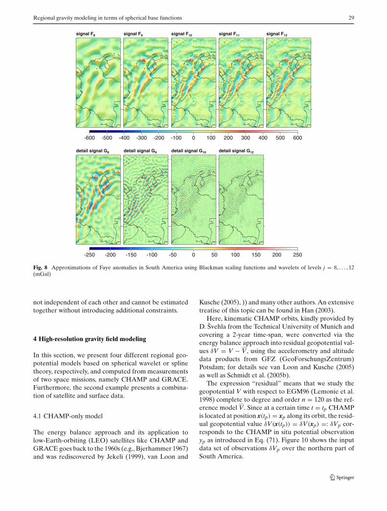
To be more specific, here we investigate an examplethat is discussed in more detail in Sect. 4.2, namely theregional recovery of the Earth’s gravity field from Fayegravity anomalies given within the Colombian region(Fig. 13). For better comparison, we computed recon-structions of the given data using all four wavelet typesintroduced at the end of Sect. 2.4. We observe that thereconstruction depends on the shape of the kernel func-tion used.

From Figs. 2, 3 and 4 we note that due to the spatiallocalization the Shannon, Blackman and CuP kernelscover approximately only a spherical cap of two degreesat level j = 8, which decreases nearly by half if thelevel is increased by one, e.g., we note from Figs. 2, 3and 4 a support diameter of about 0.5 degree for levelj = 10. This strong spatial localization effectively detectsthe small terrain-correlated details in the Faye anomalydata set.

However, we also note small differences between theapproximations of the CuP and Blackman reconstruc-tion process and the Shannon approximations. FromFig. 2, we note many ripples of the Shannon kernel thatintroduce a characteristic blurring into the approxima-tions given in Fig. 6; see particularly the panels of thedetail signals G9(x) and G10(x). This effect is also knownas spectral ringing from classical Fourier theory.

Interestingly, Figs. 7 and 8 show that this ringing canbe minimized or even avoided by taking a smooth kernelinto account. Optimal smoothness in the sense that thekernel shows no (micro-)oscillations is guaranteed bythe Bernstein kernel (Fig. 9). However, as Fig. 5 shows,the spatial localization increases slower than that of theother three examples. The consequence is a larger sup-port of the kernel leading to boundary effects. Suchboundary effects can occur as ripples or as a suddendecay to the boundary if the kernel has a support thatis much greater than the regional details to be inves-tigated. Since boundary effects are of special interestfor the detail signals of the lower levels, they disappearwhen increasing the level (not shown here).

3.2 Parameter estimation

Following Eqs. (24) and (34), the function F(x) can gen-erally be modeled as

F(x) = a(x)Tβ, (70)

wherein the N × 1 vector a(x) ∈ {b(x), krep(x)} containsthe values of the spherical base functions.

In order to estimate the unknown N × 1 coefficientvector β = c for a(x) = b(x) or β = d for a(x) =krep(x) , we need values F(xp) =: Fp of the function F(x)

in altogether P discrete observation points xp ∈ �extR

with p = 1, . . . , P and P ≥ N.Since geodetic measurements y(xp) =: yp are always

affected by measurement errors ep := e(xp), i.e. Fp =yp + ep, Eq. (70) can be rewritten as

yp + ep = aTp β (71)

with a(xp) =: ap. Introducing the P × 1 vectors y =(y1, y2, . . . , yP)

T and e = (e1, e2, . . . , eP)T of the obser-

vations and the measurement errors, respectively, theP × N coefficient matrix A = (a1, a2, . . . , aP)

T and theP × P covariance matrix D(y) of the observations, thelinear model

y + e = A β with D(y) = σ 2y P−1

y (72)

is established. Herein σ 2y and Py are denoted as the vari-

ance factor and the weight matrix, respectively; see Koch(1999).

Analogous to the matrix H (Eq. 14) and dependingon the distribution of the observation sites, the matrixA is at most of rank n, i.e., a rank deficiency of at leastN − n exists. In the following, however, we will assumethat rankA = n holds.


signal F8

detail signal G8

signal F9

detail signal G9

signal F10

detail signal G10

signal F11

detail signal G12

signal F12

-600 -500 -400 -300 -200 -100 0 100 200 300 400 500 600

-250 -200 -150 -100 -50 0 50 100 150 200 250

Fig. 6 Approximations of Faye anomalies in South America using Shannon scaling functions and wavelets of levels j = 8, . . . , 12 (mGal)

Besides the rank deficiency problem, the normalequation system following from the application of theleast-squares method to the linear model (Eq. 72) mightbe ill-conditioned. If we, e.g., want to compute the grav-ity field at the Earth’s surface only from satellite data,this inverse problem requires regularization. Here, wesolve both problems, the rank deficiency and the regu-larization, together.

If we assume that prior information for the expec-tation vector E(β) = µβ and the covariance matrixD(β) = P−1

β of the vector β is available, the additionallinear model

µβ + eβ = β with D(µβ) = σ 2β P−1

β (73)

can be formulated. Herein, eβ is defined as the errorvector of the prior information and σ 2

β the correspond-ing unknown variance factor. The combination of thetwo models (Eqs. 72 and 73) gives an extended linearmodel with unknown variance components σ 2

y and σ 2β ,

namely

[yµβ

]

+[

eeβ

]

=[

AI

]

β with

D( [

yµβ

])

= σ 2y

[P−1

y 00 0

]

+ σ 2β

[0 00 P−1

β

]

.

(74)

The application of the least-squares method to thismodel yields the normal equations

(ATPy A + λPβ) β = ATPy y + λPβ µβ (75)

with the regularization parameter λ := σ 2y /σ

2β . The

method of estimating variance components (e.g., Koch1999) allows the computation of an estimator of λ bymeans of

σ 2y = (eTPy e)/ry , (76)

σ 2β = (eT

βPβ eβ)/rβ . (77)


signal F8

detail signal G8

signal F9

detail signal G9

signal F10

detail signal G10

signal F11

detail signal G12

signal F12

-600 -500 -400 -300 -200 -100 0 100 200 300 400 500 600

-250 -200 -150 -100 -50 0 50 100 150 200 250

Fig. 7 Approximations of Faye anomalies in South America using CuP scaling functions and wavelets of levels j = 8, . . . , 12 (mGal)

Herein e and eβ denote the residual vectors as well asry and rβ the partial redundancies, i.e., the contributionsof the observations and the prior information to thetotal redundancy r = ry + rβ = P of the linear model(Eq. 74).

Thus, the unbiased estimator

β = (ATPy A + λPβ)−1 (AT Py y + λPβ µβ) (78)

with the covariance matrix

D(β) = σ 2y (A

TPy A + λPβ)−1 (79)

is obtained from Eq. (75) if the variance component esti-mation converges. In the case β = d = dJ , the estimatordJ is the starting point of the MRR as mentioned in thecontext of Fig. 1. Note, that the covariance matrices ofall coefficient vectors dj and all detail signals Gj(x) arecalculable from the covariance matrix D(β) applying thelaw of error propagation.

The procedure described here allows the combinationof different kinds of measurements, e.g., gravity anoma-lies and potential values. Then additional operators, likethe Stokes operator, have to be considered in the vectorap of Eq. (71). In opposite to that the numerical integra-tion, discussed in the previous subsection, is restrictedto one single type of observation, e.g., gravity anomalies(e.g., Torge 2001).

A theoretical study on the condition number of the(regularized) normal matrix in Eq. (75) and its depen-dency from the chosen point system and the base func-tion type, has been conducted by Kusche (2002).

One also may desire an estimation of the detail signalsGj(x) for j = j′, . . . , J directly from Eq. (50). However,it follows from Eq. (52), that e.g., in the Blackman case(Eqs. 63 and 64) the wavelet functions �Bla

j (x, xk) and

�Blaj+1(x, xk) of two consecutive levels j and j + 1 over-

lap in the spectral domain. Thus, according to Eq. (49)the corresponding detail signals Gj(x) and Gj+1(x) are


signal F8

detail signal G8

signal F9

detail signal G9

signal F10

detail signal G10

signal F11

detail signal G12

signal F12

-600 -500 -400 -300 -200 -100 0 100 200 300 400 500 600

-250 -200 -150 -100 -50 0 50 100 150 200 250

Fig. 8 Approximations of Faye anomalies in South America using Blackman scaling functions and wavelets of levels j = 8, . . . , 12(mGal)

not independent of each other and cannot be estimatedtogether without introducing additional constraints.

4 High-resolution gravity field modeling

In this section, we present four different regional geo-potential models based on spherical wavelet or splinetheory, respectively, and computed from measurementsof two space missions, namely CHAMP and GRACE.Furthermore, the second example presents a combina-tion of satellite and surface data.

4.1 CHAMP-only model

The energy balance approach and its application tolow-Earth-orbiting (LEO) satellites like CHAMP andGRACE goes back to the 1960s (e.g., Bjerhammer 1967)and was rediscovered by Jekeli (1999), van Loon and

Kusche (2005), )) and many other authors. An extensivetreatise of this topic can be found in Han (2003).

Here, kinematic CHAMP orbits, kindly provided byD. Švehla from the Technical University of Munich andcovering a 2-year time-span, were converted via theenergy balance approach into residual geopotential val-ues δV = V − V, using the accelerometry and altitudedata products from GFZ (GeoForschungsZentrum)Potsdam; for details see van Loon and Kusche (2005)as well as Schmidt et al. (2005b).

The expression “residual” means that we study thegeopotential V with respect to EGM96 (Lemonie et al.1998) complete to degree and order n = 120 as the ref-erence model V. Since at a certain time t = tp CHAMPis located at position x(tp) = xp along its orbit, the resid-ual geopotential value δV(x(tp)) = δV(xp) =: δVp cor-responds to the CHAMP in situ potential observationyp as introduced in Eq. (71). Figure 10 shows the inputdata set of observations δVp over the northern part ofSouth America.


signal F8

detail signal G8

signal F9

detail signal G9

signal F10

detail signal G10

signal F11

detail signal G12

signal F12

-100 -80 -60 -40 -20 0 20 40 60 80 100

-50 -40 -30 -20 -10 0 10 20 30 40 50

Fig. 9 Approximations of Faye anomalies in South America using Bernstein scaling functions and wavelets of levels j = 8, . . . , 12(mGal)

We identify the right-hand side of the observationequation (Eq. 71) with the right-hand side of Eq. (34),i.e., we set aT

pβ =: krep(xp)Td. For the MRR of the input

data, we select the Blackman scaling function definedby its Legendre coefficients

�j;n =: �Blaj;n =

1 if n ∈ [0, bj−1)

Aj(n) if n ∈ [bj−1, bj)

0 else

, (80)

wherein

Aj(n) = 2150

− 12

cos

(2πnj

bj

)

+ 225

cos

(4πnj

bj

)

(81)

with nj = n+�bj�−2 · �bj−1�, bj = 2 · (bj −bj−1) and b ∈R

+. Recall that in Eq. (63) the Blackman scaling func-tion was already presented for b = 2. Due to Eq. (52)each Blackman wavelet functionψBla

j (x, xk) is related to

a specific frequency band Bj := {n | bj−1 ≤ n < bj+1}and therefore strictly band-limited. With b = 1.55 andJ = 11, the level-11 wavelet function covers the fre-quency range between spherical harmonics n = 80 andn = 192, i.e., we solve for signal parts up to degreen = n11 = 192 and set n′ = n11 in Eq. (30).

We relate the coefficients dk of the vector d = β to thepoints xk (Eq. 67) of a standard longitude–latitude gridwithin the computation window shown in Fig. 10. Thespacing of the grid points is chosen such that the corre-sponding global point system SN11 is admissible accord-ing to Eq. (16).

Since we expect less variability in the residual geo-potential for oceanic regions than for the continents, wesubdivide the vector β into a sub-vector β1 collectingthe coefficients dk related to the grid points xk of theoceanic area and a second sub-vector β2 for the corre-sponding coefficients over land; note that as an option,the coastal area might be considered by a third sub-vector. We want to emphasize explicitly that splitting


-10

0

10

280 290 300 310

-3.0 -1.5 0.0 1.5 3.0

[ m2/s2 ]

Fig. 10 Satellite input data set: CHAMP in situ potential overthe northern part of South America; EGM96 up to degree andorder n = 120 is subtracted. In order to reduce boundary effects,the real data window is a little bit larger than the computationwindow shown here. The data was computed and kindly providedby J. van Loon, Technical University of Delft

the prior information into different spatial subregionsmeans a space-dependent regularization.

We introduce the prior information µβ1= 0 and

µβ2= 0 for the expectation vectors as well as Pβ1 = I

and Pβ2 = I for the inverse covariance matrices. We usea fast Monte-Carlo implementation of the iterative max-imum likelihood variance component estimation (Kochand Kusche 2001) and obtain the estimators β = d, σ 2

y ,σ 2β1

and σ 2β2

following Eqs. (76) to (78). The estimatorσ 2β2

is about twenty times larger than the estimated var-iance component σ 2

β1, i.e., as expected the linear model

(Eq. 73) for the prior information causes a much stron-ger regularization for the oceanic regions than for thecontinent. Furthermore, from Eq. (79), we obtain anestimation of the covariance matrix D(d).

As mentioned before, the estimated coefficient vectord = d11 is the input quantity of the MRR shown in Fig. 1.The estimated detail signals Gj(x) up to level j = 11(not shown here) are computed according to Eq. (56)and transferred into the detail signals ζj(x) =: ζ cha

j (x) ofheight anomalies following Molodensky’s theory (e.g.,Heiskanen and Moritz 1967). The corresponding covari-ance matrices are calculable as mentioned in the contextof Eq. (79).

-10

0

10

280 290 300 310

-5 -4 -3 -2 -1 0 1 2 3 4 5

[ m ]

Fig. 11 Estimated residual height anomalies δζ cha(x) from theCHAMP Blackman wavelet model: residual to EGM96 to degreeand order n = 120

Figure 11 shows the estimated residual height anom-alies

δζ cha(x) =11∑

j=2

ζ chaj (x). (82)

By adding the corresponding height anomalies ζ (x) fromEGM96 up to degree n = 120 we finally obtain the esti-mated height anomalies ζ cha(x) = ζ (x)+ δζ cha(x).

In order to check the quality of the wavelet repre-sentation, we compare the CHAMP Blackman wave-let model (Eq. 82) with the corresponding values ofthe GRACE-only EIGEN-GRACE02S global spheri-cal harmonic model from GFZ (Reigber et al. 2005).As can be seen from Figs. 11 and 12, there is a verygood agreement between the two models; the RMSvalue of the differences amounts 0.5 m, the correlation isapproximately 0.72. We believe the main reason forthese promising results is the space-dependent regu-larization mentioned before instead of the frequency-dependent regularization usually performed within thespherical harmonic approach.

A similar study of the same input data set was per-formed by Schmidt et al. (2005b). In contrast to ourinvestigations here, they used numerical integrationtechniques and did not apply a regularization pro-cedure. They derived a so-called multi-level wavelet


-10

0

10

280 290 300 310

-5 -4 -3 -2 -1 0 1 2 3 4 5

[ m ]

Fig. 12 Residual height anomalies computed from GFZ’sGRACE-only EIGEN-GRACE02S gravity field model (EGM96up to degree n = 120 is subtracted)

representation of geoid undulations, i.e. they introduceddifferent “highest” resolution levels for the oceans andthe continent, respectively.

4.2 Combined model from CHAMP and surface data

In order to establish a high-resolution gravity model, wehave to combine satellite data with surface data, sincedifferent measurement types generally cover differentparts of the frequency spectrum (e.g., Kern et al. 2003).Satellite data provide the low- and medium-frequencyinformation of the geopotential, whereas local orregional surface data cover the medium- and remain-ing high-frequency parts.

As surface data, we analyze a high-resolution data setcontaining 2′ × 2′ mean Faye gravity anomalies referredto ground level (Fig. 13). This data set has been derivedfrom terrestrial and aerial gravity measurements(Sánchez 2003) and complemented by altimetry grav-ity anomalies of Sandwell and Smith (1997) [gravitydata (2′ × 2′ grid), version 10.2] in marine areas. Again,EGM96 complete to degree n = 120 is removed as thereference field (Fig. 13). Recall that this data set wasalready used in Sect. 3.1 for studying the different scalingand wavelet functions introduced at the end of Sect. 2.4.

By means of FFT-based numerical integration tech-niques, already mentioned in Sect. 3.1, the decomposi-tion into detail signals ζ sur

j (x) of height anomalies for

-4

-2

0

2

4

6

8

10

12

14

284 286 288 290-600

-450

-300

-150

0

150

300

450

600[ mGal ]

Fig. 13 Surface input data set: 2′ × 2′ mean Faye gravity anoma-lies over Colombia; EGM96 up to degree n = 120 is subtracted

levels j = 9, . . . , 18 (not shown here) is performed againusing the Blackman wavelet function with b = 1.55.Hence, the detail signal of level j = 18 contains signalparts up to degree n = 4, 133. As mentioned before, alevel-combination strategy has to be applied in orderto derive the high-resolution gravity model, generallyformulated as

ζ(x) = ζ (x)+J∑

j=j′wcha

j ζ chaj (x)+

J∑

j=j′wsur

j ζ surj (x) (83)

for the height anomaly ζ(x).The level weights wcha

j and wsurj are restricted to 0 ≤

wchaj ≤ 1, 0 ≤ wsur

j ≤ 1 and

wchaj + wsur

j = 1 for j = j′, . . . , J. (84)

Using the degree variances σ 2n (F), introduced in the con-

text of Eq. (8), and the corresponding error degree vari-ances ε2

n(F), the Wiener filter curve values pn(F) of a sig-nal F are defined as pn(F) = σ 2

n (F)/(σ2n (F)+ε2

n(F)) (e.g.,Wang 1993, Kern et al. 2003). Here we use the Wienerfilter curve of GFZ’s EIGEN-CHAMP03S model anddetermine the satellite level weights wcha

j for j = 9, 10, 11


0.0

0.2

0.4

0.6

0.8

1.0

1.2va

lue

0 3 6 9 12 15 18

level

Fig. 14 Level weights wchaj (circles) and wsur

j (triangles) of thedetail signals in Eq. (83) with j′ = 1 and J = 18

-4

-2

0

2

4

6

8

10

12

14

282 284 286 288 290-50

-40

-30

-20

-10

0

10

20

30

40

50[ m ]

Fig. 15 High-resolution gravity field model [in terms of heightanomalies (m)] of Colombia computed according to Eq. (83) withj′ = 2 and J = 18. The model contains signal parts up to degreen = 4, 133

according to the formula

wchaj =

n′

∑

n=0

pn(F) �Blaj;n

/

n′

∑

n=0

�Blaj;n

; (85)

Figure 14 displays the numerical values of the levelweights wcha

j and wsurj according to Eqs. (84) and (85).

Figure 15 shows the height anomalies ζ(x) of the high-resolution gravity field model of Colombia according toEq. (83) with j′ = 2 and J = 18.

In contrast to the procedure described before,Schmidt et al. (2005b) computed a high-resolution grav-ity field model without applying a combination strategy.In other words, they chose level weights wcha

j = 1 and

wsurj = 0 for the satellite part as well as wcha

j = 0 andwsur

j = 1 for the remaining levels computed from surfacedata.

4.3 GRACE-only model

The approach presented here for deriving a geopotentialmodel from GRACE data is based on a combined repre-sentation of spherical harmonics and harmonic splinesas space-localizing base functions. It integrates a globalgravity field recovery with regional gravity field refine-ments tailored to the local gravity field features. In a firststep, the gravity field up to a moderate spherical har-monic degree is recovered; the individual gravity fieldcharacteristics in areas of rough gravity field signals aremodeled subsequently by space localizing base functionsin a second step.

The observation equation is based on an adjustmentof the functional model that has been successfully appliedto CHAMP data (Mayer-Gürr et al. 2005). It is a Fred-holm integral equation of the first kind in the timedomain, which represents a solution of a boundary-valueproblem to Newton’s equation of motion for short arcsof the satellite orbit. For GRACE, the observations areprecise inter-satellite measurements as ranges or range-rates. Therefore, the mathematical model can be derivedby projecting the equations of relative motion to theline-of-sight connection (Mayer-Gürr et al. 2006).

The following recovery results refer to one month ofrange-rate measurements in August 2003. From this dataset, first a global solution was calculated up to degree n =90. For the regional refinement solutions, the same math-ematical model as used for the global solution has beenapplied except for the gravity field representation. Thedisturbing potential is now modeled by space-localizingbase functions according to Eq. (18), with the unknowncoefficients ck of the N × 1 vector c = β. The basefunctions, as given by Eq. (19), are located on a regulargrid generated by a uniform densification of an icosahe-dron of 20 spherical equal-area triangles. This densifiedgrid has a mean distance between the nodal points ofapproximately 160 km.

According to Eq. (19), the Legendre coefficients Bn

represent the frequency behavior of the base functions.As already explained in the context of Eq. (29), thesecoefficients can be related to the power spectrum of thesignal that is to be modeled. Consequently, up to degreen = 90, the error degree variances ε2

n(F), as introduced


-30 -30 -10 0

[cm]10 20 30

Fig. 16 Differences in geoid heights between the GRACE splinesolution of August 2003 and EIGEN-CG03C; the RMS value ofthe differences amounts to 7.1 cm

in the context of Eq. (85), of our global solution wereused for Bn as they represent the signal that is still in thedata in addition to the global solution. Above n = 90,the degree variances σ 2

n (F) were calculated accordingto Kaula’s (1966) rule of thumb. The maximum degreen′ should correspond to the envisaged maximum reso-lution expected for the regional recovery; thus, in thefollowing examples this maximum degree is selected asn′ = 120, i.e.

Bn =

√4πR2

2n+1 εn(F) if n ∈ [0, 90]GM

√4π

2n+110−5

n2 if n ∈ [91, 120]0 else

(86)

with GM being the product of the gravitational constantand the total mass of the Earth. To account for the ill-posedness of the downward continuation procedure, themethod of estimating variance components is applied asalready explained in Sect. 3.2 and applied in Sect. 4.1.

Figure 16 shows the differences in geoid heights of aregional refined spline solution calculated from 1 monthof GRACE data compared to GFZ’s combination modelEIGEN-CG03 (Förste et al. 2005). The latter is based onone year of GRACE data, additional CHAMP and sur-face data. Thus, although considerably less data has beenused for our spline solution, an RMS value of 7.1 cm forthe differences is rather small.

-30 -20 -10 0

[cm]10 20 30

Fig. 17 Differences in geoid heights between GFZ’s GRACEsolution for August 2003 and EIGEN-CG03C; the RMS value ofthe differences amounts to 9.3 cm

Figure 17 displays as a comparison the differencesbetween the EIGEN-CG03C and a monthly solutioncalculated by GFZ for August 2003; the correspondingRMS value amounts 9.3 cm. The stripes apparent in theresidual fields may result from time-variable effects, e.g.,caused by the atmosphere, that have not been modeledsufficiently. Also, due to the GRACE measurement con-figuration, random noise results in stripes.

Subsequently, regional refinements with an altogetherglobal coverage can be merged by means of quadraturemethods to obtain a globally refined solution withoutany stability problems; see Eicker et al. (2006). Usingregional “zoom-ins” to calculate a global gravity fieldis a reasonable alternative to the direct computation ofthe potential coefficients since the regionally adaptedrecovery procedure allows for extra information to beextracted out of the given data set. In particular, it hasto be pointed out that – according to Eq. (75) – the reg-ularization parameter λ is individually determined foreach regional solution. A global regularization causesan overall filtering of the observations leading to a meandampening of the global gravity field features. By aregionally adapted regularization, it is possible to extractmore information out of the given data than wouldbe possible with a global gravity field determination.Regions with a smooth gravity field signal for instancecan be regularized more strongly without dampeningthe signal. In addition, the resolution of the gravity fielddetermination can be chosen for each region individu-


ally according to the spectral behavior of the signal. Thiskind of space-dependent regularization was already dis-cussed in Sect. 4.1.

4.4 Spatio-temporal GRACE-only model

In Sect. 4.1, we analyzed residual geopotential valuesδV(x(tp)) derived from CHAMP applying the energybalance approach. Assuming now that at time t = tp thetwo GRACE satellites are located at the positions x1(tp)and x2(tp) along their orbits, the difference �V1,2(tp) =δV(x1(tp))−δV(x2(tp))means the GRACE in situ poten-tial difference observation. Here, we define the resid-ual geopotential values δV(xi(tp)) with i ∈ {1, 2} as thedifference between the geopotential V at position xi(tp)and the corresponding value V of the complete expan-sion of the GGM01C gravity model (Tapley et al. 2004a)chosen as the reference.

As explained by Han et al. (2006) in detail, the poten-tial difference �V1,2(t) can be computed by combiningthe inter-satellite range-rate, the position, velocity andacceleration data of the two GRACE satellites againthrough the energy balance approach. The observationequation for a single observation �V1,2(tp) =: y(tp) isgiven by Eq. (71) with ap = krep(x1(tp))−krep(x2(tp)) =:a1,2 and β = d(tp), i.e.

y(tp)+ e(tp) = aT1,2 d(tp) . (87)

As mass variations due to atmosphere, tidal and non-tidal ocean variabilty are considered during the pre-processing steps, the observations y(tp) should mainlyreflect the variations in continental water storage.

Our objective is now the computation of time-depen-dent geoid undulations δN(x, t). Analogous to Eq. (82),we introduce the spatio-temporal MRR

δN(x, t) =J∑

j=j′Nj(x, t) (88)

with detail signals Nj(x, t). By adding the correspondingvalues N(x) of the static reference model GGM01C, weobtain the geoid undulations N(x, t) = N(x)+ δN(x, t).

Our study is again related to the northern part ofSouth America, including the Amazon basin. The datacovers the time span between February and December2003, except June 2003. In the following, the procedureto estimate the detail signals Nj(x, t) from the GRACEdata is described briefly; for more details see Schmidt etal. (2006).

First, we choose again the Blackman scaling functiondefined in Eqs. (80) and (81) with b = 2.3 and highest

Table 1 Level-dependent observation period, total number ofobservations within the corresponding time-span and highestdegree value n related to the level−j Blackman scaling functionwith base b = 2.3 according to Eqs. (80) and (81)

Level Observation Number of Highestj period observations degree

2 10 days ≈ 5,000 123 1 month ≈ 15,000 274 3 months ≈ 25,000 64

resolution level J = 4, i.e. we solve for signal parts untildegree n = 64. Hence, in Eq. (87), we have to choosethe reproducing kernel (Eq. 30) with n′ ≥ 64. In con-trast to the procedure described in Sect. 4.1, we want toestimate the detail signals Nj(x, t) of Eq. (88) for levelsj = 2, 3, 4 from different data sets.

The idea stems from the fact that the determination offiner structures of the gravity field needs a denser distri-bution of satellite tracks than the computation of coarserstructures. Hence, the estimation of the level-4 detailsignal N4(x, t) should be based on a longer observationperiod then the level-3 detail signal N3(x, t). Table 1shows the selected information to create the differentdata sets for establishing the desired MRR (Eq. 88).

For each data set, the parameter estimation is per-formed in the same manner as described in subsec-tion 4.1, i.e., the data sets altogether provide time-seriesfor the estimators of the scaling coefficient vectors d2,d3 and d4 with a temporal resolution of 10 days, 1 monthand 3 months, respectively. The estimated detail signalsare computed according to Eq. (56) and transformedinto the detail signals Nj(x, t) =: Ngra

j (x, t) by applyingBruns’s theorem (e.g., Heiskanen and Moritz, 1967).

As an example, Fig. 18 shows the estimated detailsignals Ngra

3 (x, t) computed from ten data sets each cov-ering an observation period of one month according toTable 1. Similar results can be obtained for the remain-ing levels j = 2 and j = 4 (not shown here).

Seasonal variations of the estimated geoid undula-tions with respect to the GGM01C reference modelare clearly detectable in Fig. 18. The results agree verywell with other studies on this topic; see e.g., Tapley etal. (2004b) and Han et al. (2005). We want to empha-size that in our approach, the Gaussian kernel (see theremark at the end of Sect. 2) is replaced by the Blackmankernel defined in Eqs. (80) and (81).

According to Eq. (88), the estimated variations ofthe gravity field can be transformed, e.g., into so-calledequivalent water heights or height deformations.Schmidt et al. (2006), among others, compare theseresults with hydrological models and GPS time-seriesof height variations.


February 2003 March 2003 April 2003 May 2003 July 2003

August 2003 September 2003 October 2003 November 2003 December 2003

-10 -8 -6 -4 -2 0 2 4 6 8 10

[ mm ]

Fig. 18 Monthly solutions for detail signal N3(x, t) of the residual geoid undulations δN(x, t) according to Eq. (88); the results arecomputed from GRACE data using the Blackman wavelet function with base b = 2.3

5 Summary and conclusions

We have demonstrated that spline and wavelet tech-niques can be successfully applied to regional satellitedata collected from the current CHAMP and GRACEgravity missions. We also addressed the combination ofsatellite and surface gravity data sets by using an appro-priate weighting scheme, as well as the establishmentof a spatio-temporal approach. In order to demonstratethe power of such modeling, different regional gravityrepresentations of the northern part of South Americahave been derived and discussed.

One important result is the improvement of the grav-ity field using regional techniques in comparison withthe corresponding parts of global spherical harmonicmodeling. It was demonstrated that a regional wave-let CHAMP-only model fits the corresponding part ofa global spherical harmonic GRACE-only model verywell. The reason can be seen in the spatial regularizationinstead of the classical regularization in the frequency-domain. In addition, regional models with a globalcoverage can be merged to obtain a globally refinedsolution.

The multi-resolution representation allows theconstruction of the gravity field by detailed signals ormodules. These modules are basically computable bydifferent data sets. In spatio-temporal modeling, thisprocedure allows the computation of detailed signalsfrom data sets both covering different parts of the fre-quency spectrum and spanning different observation

intervals. Hence, this procedure means a model improve-ment with respect to the usual computation of time-var-iable gravity fields spanning fixed time intervals of, e.g.,1 month.

Acknowledgments We are grateful to GeoForschungsZentrum(GFZ) Potsdam for providing CHAMP data through their Infor-mation System and Data Center (ISDC). Thanks go also to DrazenŠvehla (Technical University of Munich) for providing CHAMPkinematic orbits and to Jasper van Loon (Technical Universityof Delft) for processing the kinematic orbits via the energybalance approach. The authors would like to thank the anony-mous reviewers for their helpful comments to improve thepaper.

References

Bjerhammer A (1967) On the energy integral for satellites. Rep.of the R. Inst. of Techn. Sweden, Stockholm

Cui J (1995) Finite pointset methods on the sphere and theirapplication in physical geodesy. PhD thesis, University ofKaiserslautern, Mathematics Department, Geomathemat-ics Group

Driscoll JR, Healy RM (1994) Computing Fourier transformsand convolutions on the 2-sphere. Adv Appl Math 15:202–250

Eicker A, Mayer-Gürr T, Ilk K-H (2006) A global CHAMPgravity field by merging of regional refinement patches.Adv Geosci (submitted) (Proceedings of the JointCHAMP/GRACE Science Meeting)

Fengler MJ (2005) Vector spherical harmonic and vector wave-let based non-linear Galerkin schemes for solving theincompressible Navier-Stokes equation on the sphere. PhD


thesis (submitted), University of Kaiserslautern, Mathemat-ics Department, Geomathematics Group

Fengler MJ, Freeden W, Gutting M (2004a) The Kaiserslauterngeopotential model SWITCH-03 from Orbit Pertubationsof the Satellite CHAMP and its comparison to the mod-els EGM96, UCPH2002_02_0.5, EIGEN-1S, and EIGEN-2.Geophys J Int 157:499–514

Fengler MJ, Freeden W, Kusche J (2004b) Multiscale geo-potential solutions from CHAMP orbits and accelerom-etry. In: Reigber C, Lühr H, Schwintzer P, Wickert J(eds) Earth observation with CHAMP, results from threeyears in orbit. Springer, Berlin Heidelberg New York,pp 139–144

Fengler MJ, Freeden W, Gutting M (2005) The spherical Bern-stein wavelet. Schriften zur Funktionalanalysis und Geo-mathematik, 20, University of Kaiserslautern, MathematicsDepartment, Geomathematics Group

Fengler MJ, Michel D, Michel V (2006a) Harmonic spline-wavelets on the 3-dimensional ball and their applicationto the reconstruction of the Earth’s density distributionfrom gravitational data at arbitrarily shaped orbits. ZAMM(accepted)

Fengler MJ, Freeden W, Kohlhaas A, Michel V, Peters T (2006b)Wavelet modelling of regional and temporal variations ofthe Earth’s gravitational potential observed by GRACE. JGeod (accepted)

Förste C, Flechtner F, Schmidt R, Meyer U, StubenvollR, Barthelmes F, König R, Neumayer K-H, Rothacher M,Reigber Ch, Biancale R, Bruinsma S, Lemoine J-M, Rai-mondo JC (2005) A new high resolution global gravity fieldmodel derived from combination of GRACE and CHAMPmission and altimetry/gravimetry surface gravity data. Pre-sented at EGU General Assembly 2005, Vienna, Austria

Freeden W (1981) On approximation by harmonic splines.manuscr geod 6:193–244

Freeden W (1999) Multiscale modelling of spaceborne geodata.Teubner, Stuttgart

Freeden W, Schreiner M (1995) New wavelet methods forapproximating harmonic functions. In: Sansò F (ed) Geo-detic theory today. Springer, Berlin Heidelberg New York,pp 112–121

Freeden W, Windheuser U (1996) Spherical wavelet transformand its discretization. Adv Comput Math 5:51–94

Freeden W, Michel V (2004) Multiscale potential theory(with applications to Earth’s sciences). Birkhäuser Verlag,Boston

Freeden W, Gervens T, Schreiner M (1998a) Constructiveapproximation on the sphere (with applications to geomath-ematics). Clarendon Press, Oxford

Freeden W, Glockner O, Schreiner M (1998b) Spherical panelclustering and its numerical aspects. J Geod 72:586–599

Freeden W, Michel D, Michel V (2005) Local multiscale approx-imations of geostrophic flow: theoretical background andaspects of scientific computing. Mar Geod 28:313–329

Han SC (2003) Efficient global gravity determination fromsatellite-to-satellite tracking (SST). PhD thesis, Geodeticand Geoinformation Science, Department of Civil and Envi-ronmental Engineering and Geodetic Science, The OhioState University, Columbus

Han SC, Shum CK, Jekeli C, Alsdorf D (2005) Improved esti-mation of terrestrial water storage changes from GRACE.Geophys Res Lett 32:L07302. DOI 10.1029/2005GL022382

Han SC, Shum CK, Jekeli C (2006) Precise estimation of in situgeopotential differences from GRACE low-low satellite-to-satellite tracking and accelerometry data. J Geophys Res111:B4411. DOI 10.1029/2005JB003719

Heiskanen W, Moritz H (1967) Physical geodesy. Freeman, SanFrancisco

Holschneider M, Chambodut A, Mandea M (2003) From globalto regional analysis of the magnetic field on the sphere usingwavelet frames. Phys Earth Planet Int 135:107–124

Ilk KH, Löcher A (2005) The use of the energy balance relationsfor validation of gravity field models and orbit determina-tion. In: Sansò F (ed) A window on the future of geodesy.Springer, Berlin Heidelberg New York, pp 494–499

Jekeli C (1981) Alternative methods to smooth the Earth’s grav-ity field. Report 327, Department of Geodetic Science, TheOhio State University, Columbus

Jekeli C (1999) The determination of gravitational potentialdifferences from satellite-to-satellite tracking. Cel MechDyn Astr 75:85–100

Kaula WM (1966) Theory of satellite geodesy. Blaisdell,Waltham

Kern M, Schwarz KP, Sneeuw N (2003) A study on the com-bination of satellite, airborne, and terrestrial gravity data. JGeod 77:217–225

Koch KR (1999) Parameter estimation and hypothesis testingin linear models. Springer, Berlin Heidelberg New York

Koch KR, Kusche J (2001) Regularization of geopotential deter-mination from satellite data by variance components. JGeod 76:259–268

Kusche J (2002) Inverse Probleme bei der Gravitationsfeldbes-timmung mittels SST- und SGG-Satellitenmissionen. Ger-man Geodetic Commission, Series C, 548, Munich

Lemoine FG, Kenyon SC, Factor JK, Trimmer RG, Pavlis NK,Chinn DS, Cox CM, Klosko SM, Luthcke SB, Torrence MH,Wang YM, Williamson RG, Pavlis EC, Rapp RH, OlsonTR (1998) The development of the joint NASA GSFC andthe National Imagery and Mapping Agency (NIMA) geo-potential model EGM96, NASA/TP-1998-206861, NationalAeronautics and Space Administration, Maryland

Li TH (1999) Multiscale representation and analysis of sphericaldata by spherical wavelets. SIAM J Sci Comput 21:924–953

van Loon J, Kusche J (2005) Stochastic model validation ofsatellite gravity data: A test with CHAMP pseudo-obser-vations. In: Jekeli C, Bastos L, Fernandes J (eds) Grav-ity, geoid and space missions. Springer, Berlin HeiodelbertgNew York, pp 24–29

Maier T (2005) Wavelet-Mie-representations for solenoidal vec-tor fields with applications to ionospheric geomagnetic data.J Appl Math 65:1888–1912

Marchenko AN (1998) Parameterization of the Earth’s gravityfield – Point and line singularities. Lviv Astronomical andGeodetic Society, Lviv

Mautz R, Schaffrin B, Shum CK, Han SC (2004) Regionalgeoid undulations from CHAMP represented by locallysupported basis functions. In: Reigber C, Lühr H,Schwintzer P, Wickert J (eds) Earth observation withCHAMP, results from three years in orbit. Springer, Ber-lin Heidelberg New York, pp 230–236

Mayer C (2004) Wavelet modelling of the spherical inversesource problem with application to geomagnetism. Inverseproblems 20:1713–1728

Mayer-Gürr T, Ilk KH, Eicker A, Feuchtinger M (2005) ITG-CHAMP01: a CHAMP gravity field model from short kine-matical arcs of a one-year observation period. J Geod78:462–480

Mayer-Gürr T, Eicker A, Ilk KH (2006) Gravity field recoveryfrom GRACE-SST data of short arcs. In: Flury J, Rummel R,Reigber C, Rothacher M, Boedecker G, Schreiber U (eds)Observation of the Earth system from Space. Springer, Ber-lin Heidelberg New York, pp 131–148


Mertins A (1999) Signal analysis: wavelets, filter banks, time-frequency transforms and applications. Wiley, Chichester

Moritz H (1980) Advanced physical geodesy. Wichmann,Karlsruhe

Narcowich FJ, Ward JD (1996) Nonstationary wavelets on them-sphere for scattered data. Appl Comput Harmon Anal3:324–336

Panet I, Jamet O, Diament M, Chambodut A (2005) Modellingthe Earth’s gravity field using wavelet frames. In: Jekeli C,Bastos L, Fernandes J (eds) Gravity, geoid and space mis-sions. Springer, Berlin Heidelberg New York, pp 48–53

Pavlis NK, Holmes SA, Kenyon SC, Schmidt D, Trimmer R(2005) A preliminary gravitational model to degree 2160.In: Jekeli C, Bastos L, Fernandes J (eds) Gravity, geoidand space missions. Springer, Berlin Heidelberg New York,pp 18–23

Reigber C, Schmidt R, Flechtner F, König R, Meyer U, Neuma-yer KH, Schwintzer P, Zhu SY (2005) An Earth gravity fieldmodel complete to degree and order 150 from GRACE:EIGEN-GRACE02S. J Geodyn 39(1):1–10

Sánchez L (2003) Bestimmung der Höhenreferenzfläche für Ko-lumbien. Diploma thesis. Institute of Planetary Geodesy,Technical University of Dresden

Sandwell DT, Smith WHF (1997) Marine gravity anomalyfrom Geosat and ERS-1 satellite altimetry. J Geophys Res102(B5):10039–10054 (http://topex.ucsd.edu/www_html/mar_grav.html)

Sansò F, Tscherning CC (2003) Fast spherical collocation: theoryand examples, J Geod 77:101–112. DOI 10.1007/s00190-002-0310-5

Schmidt M, Fabert O, Shum CK (2005a) Towards the estima-tion of a multi-resolution representattion of the gravity fieldbased on spherical wavelets. In: Sansò F (ed) A windowon the future of geodesy. Springer, Berlin Heidelberg NewYork, pp 362–367

Schmidt M, Kusche J, van Loon J, Shum CK, Han SC, FabertO (2005b) Multi-resolution representation of regional grav-ity data. In: Jekeli C, Bastos L, Fernandes J (eds) Gravity,Geoid and space missions. Springer, Berlin Heidelberg NewYork, pp 167–172

Schmidt M, Fabert O, Shum CK (2005c) On the estimation ofa multi-resolution representation of the gravity field basedon spherical harmonics and wavelets. J Geodyn 39:512–526

Schmidt M, Han SC, Kusche J, Sánchez L, Shum CK (2006)Regional high-resolution spatiotemporal gravity modelingfrom GRACE data using spherical wavelets. Geophys ResLett 33:L08403. DOI 10.1029/2005GL025509

Schneider F (1996) The solution of linear inverse problems insatellite geodesy by means of spherical spline approxima-tion. J Geod 71(1):2–15

Swenson S, Wahr J (2002) Methods for inferring regionalsurface-mass anomalies from satellite measurements oftime variable gravity. J Geophys Res 107(B9):2193. DOI10.1029/2001JB000576

Tapley BD, Bettadpur S, Watkins M, Reigber C (2004a) Thegravity recovery and climate experiment: mission over-view and early results. Geophys Res Lett 31:L06619. DOI10.1029/2003GL019285

Tapley BD, Bettadpur S, Ries J, Thompson P, Watkins M (2004b)GRACE measurements of mass variability in the Earth sys-tem. Science 305:503–505

Torge W (2001) Geodesy. de Gruyter, BerlinWahr J, Molenaar M, Bryan F (1998) Time variability of the

earth’s gravity field: hydrological and oceanic effects andtheir possible detection using GRACE. J Geophys Res103(B12):30205–30229

Wang Y-M (1993) On the optimal combination of potentialcoefficient with terrestrial gravity data for FFT computa-tions. manuscr geod 18:406–416

Documents

Regional gravity modeling in terms of spherical base functions · e-mail: [email protected] A. Eicker e-mail: [email protected] J. Kusche Delft Institute of Earth