RESEARCH SEMINAR IN INTERNATIONAL ECONOMICS

Gerald R. Ford School of Public Policy The University of Michigan

Ann Arbor, Michigan 48109-3091

Discussion Paper No. 673

Regional Effects of Exchange Rate Fluctuations

Christopher L. House University of Michigan and NBER

Christian Proebsting

Ecole Polytechnique Federale de Lausanne

Linda L. Tesar University of Michigan and NBER

July 2019

Recent RSIE Discussion Papers are available on the World Wide Web at: http://www.fordschool.umich.edu/rsie/workingpapers/wp.html

NBER WORKING PAPER SERIES

REGIONAL EFFECTS OF EXCHANGE RATE FLUCTUATIONS

Christopher L. HouseChristian Proebsting

Linda L. Tesar

Working Paper 26071http://www.nber.org/papers/w26071

NATIONAL BUREAU OF ECONOMIC RESEARCH1050 Massachusetts Avenue

Cambridge, MA 02138July 2019

We thank Antoine Martin, Kenneth West, George Alessandria and participants of the 50th anniversary of the JMCB conference for helpful suggestions and advice. We gratefully acknowledge financial support from the Michigan Institute for Teaching and Research in Economics (MITRE). The views expressed herein are those of the authors and do not necessarily reflect the views of the National Bureau of Economic Research.

NBER working papers are circulated for discussion and comment purposes. They have not been peer-reviewed or been subject to the review by the NBER Board of Directors that accompanies official NBER publications.

© 2019 by Christopher L. House, Christian Proebsting, and Linda L. Tesar. All rights reserved. Short sections of text, not to exceed two paragraphs, may be quoted without explicit permission provided that full credit, including © notice, is given to the source.

Regional Effects of Exchange Rate FluctuationsChristopher L. House, Christian Proebsting, and Linda L. TesarNBER Working Paper No. 26071July 2019JEL No. F22,F41,F45

ABSTRACT

We exploit differences across U.S. states in terms of their exposure to trade to study the effects of changes in the exchange rate on economic activity at the business cycle frequency. We find that a depreciation in the state-specific trade-weighted real exchange rate is associated with an increase in exports, a decline in unemployment and an increase in hours worked. The effect is particularly strong in periods of economic slack. We develop a multi-region model with inter-state trade and labor flows and calibrate it to match the state-level orientation of exports and the extent of labor migration and trade between states. The model replicates the relationship between exchange rates and unemployment. Counterfactuals show that the high degree of interstate trade plays a dominant role in transmitting shocks across states in the first year, whereas interstate migration shapes cross-sectional patterns in following years. The model suggests that a 25% Chinese import tariff on U.S. goods would be felt throughout the United States, even in states with small direct linkages to China, raising unemployment rates by 0.2 to 0.7 percentage points in the short run.

Christopher L. HouseUniversity of MichiganDepartment of Economics238 Lorch HallAnn Arbor, MI 48109-1220and NBERchouse@umich.edu

Christian ProebstingDepartment of EconomicsEcole Polytechnique Federale de LausanneCProebsting@gmail.com

Linda L. TesarDepartment of EconomicsUniversity of MichiganAnn Arbor, MI 48109-1220and NBERltesar@umich.edu

1 Introduction

This paper is motivated by three facts. First, there are large differences in the volume of trade

across states. State-level export shares range from as much as 20 percent to less than 1 percent

of state GDP. Second, export destinations also vary considerably across states. For example,

exports to Canada are systematically greater in Northern Midwest states while exports to

Mexico are more highly concentrated in the Southwest. Third, changes in real exchange

rates are frequent, large and persistent. Exchange rates of destination countries often exhibit

changes as large as 20 percent over relatively short periods of time. These basic observations

suggest that exchange rate fluctuations should have systematically different effects on each

states’ economic activity. To the extent that states are linked through trade and factor

markets, exchange rate shocks will be transmitted across state borders.

We assemble a state-level dataset to examine the relationship between state-specific trade-

weighted real exchange rates, state-level trade in goods, unemployment and output for the

years 1999-2018. We find that variations in state-level exchange rates are systematically

related to changes in the labor market. On average, a one percent exchange rate depreciation

is associated with a decrease in unemployment of roughly 0.4 percentage points and an increase

in economic activity of one to two percent. This increase in economic activity goes along with

an expansion of exports and a steady inflow of workers from other states. The strength of

these effects at the state level depends on the extent of trade exposure to a particular foreign

market. Following Ramey and Zubairy (2018), we also estimate state-dependent effects and

show that economies react stronger to exchange rate movements when local labor market

conditions are slack.

We then construct a multi-region model of the United States that is consistent with these

empirical facts. The framework builds on the multi-country DSGE model in House, Proebsting

and Tesar (2018) (HPT) that captures trade and migration flows between regions. We adapt

the HPT model to the 50 U.S. states plus the District of Columbia. The model allows for

trade in assets and goods and for migration between U.S. states. We follow the literature on

small open economies (see e.g Galı, 2008; Kehoe and Ruhl, 2009), and add a large region that

is unaffected by state-level economic developments. We refer to this region as the “rest of

the world” or RoW. The model is calibrated to match broad features of the interstate trade

statistics (Commodity Flow Statistics), labor migration data and international trade flows

at the state and country level. When feeding in the observed paths of exchange rates for

2

each state into our model, we show that our model can reproduce the effects of exchange rate

fluctuations on economic activity observed in the data.

Using the model we then explain the transmission mechanism at play: In the model, a real

exchange rate depreciation alters the relative price facing domestic firms, making the home

good cheaper for foreign consumers and boosting foreign demand. Domestic firms respond

to the higher demand by hiring more labor and expanding output. Domestic consumption

and investment rise along with the increase in employment, further stimulating the economy.

Search frictions in the labor market prevent an immediate adjustment to an efficient allocation

of labor across locations. There are two channels of transmission to those states not directly

affected by the change in the exchange rate. First, the increase in labor demand in the

affected state will trigger migration from other states. Second, because states trade with each

other, there is an indirect transmission of the exchange rate shock to demand for goods from

other states. Our counterfactuals suggest that the presence of both channels contributes to

explaining cross-sectional patterns in the data, with interstate trade playing a dominant role

in the first year after the shock and migration shaping the response in the following years.

In a next step, we ask how the last thirty years of trade globalization and the recent trade

war have left states more or less exposed to exchange rates. Since 1989, U.S. states have

steadily increased their exports (as a share of GDP), both towards traditional export markets

like Canada and the euro and to rising economies like China and Mexico. Our counterfactual

suggests that despite the increase in exports, states’ unemployment rates are not necessarily

more sensitive to foreign exchange rate fluctuations. Part of this reason is that the rise in

exports went along with higher imports and this expansion in trade offers states the ability

to use trade to limit fluctuations in local production and employment.

The recent trade war between China and the United States has seen a substantial increase

in tariffs on both sides. We use our model to evaluate the effects of an increase in Chinese

tariffs of 25% across all goods imported from the United States. In response to such a tariff,

and abstracting from higher U.S. tariffs on Chinese goods, unemployment rates are predicted

to increase by 0.2 to 0.7 percentage points across U.S. states within four quarters. Whereas

exports to China are mostly concentrated in a handfull of states in the upper Northwest, the

tariff increase will be felt throughout the United States because integrated goods and factor

markets transmit the shocks even to states that export little to China.

Our work relates to several strands of literature on the impact of trade shocks on economic

activity. Autor, Dorn and Hanson (2016) study the impact of the “China shock” on employ-

3

ment and wages in those parts of the United States specializing in sectors that compete with

Chinese imports. Caliendo, Dvorkin and Parro (2019) develop a dynamic trade model with

spatially distinct labor markets to capture the general equilibrium effects of the China trade

shock on the U.S. economy. Our paper differs from their approach by focusing on the effects

of trade shocks at the business cycle frequency.

Our paper also relates to a long-standing literature in international finance that estimates

the effect of exchange rates on economic activity (see e.g. Campa and Goldberg, 1995; Ekholm,

Moxnes and Ulltveit-Moe, 2012). We add to this literature by emphasizing how U.S. states,

though different in their direct exposure to exchange rates, are interconnected through capital

and labor markets, as well as input-output linkages that shape how states react to shocks and

how these shocks are transmitted through the U.S. economy. Finally, our paper speaks to a

recent literature in macroeconomics that has emphasized regional variation to macroeconomic

shocks in monetary unions. While HPT focuses on European countries, Beraja, Hurst and

Ospina (2016); Nakamura and Steinsson (2014); Dupor et al. (2018) have studied the conse-

quences of regional fluctuations for both regional and aggregate business cycles in the United

States.

2 Empirical Analysis

2.1 Trade Exposure Across U.S. States

We begin by examining the differences in regional exposure to trade across U.S. States and

over time. Export data by state and country of destination are drawn from the Origin of

Movement (OM) series compiled by the Foreign Trade Division of the U.S. Census Bureau.

While the series provides the most accurate available information on state export patterns, it

has two shortcomings: First, it only covers trade in manufactured and agricultural goods and

therefore excludes trade in services. At the federal level, exports of services comprise roughly

one third of all trade over our sample period. Second, the OM series credits exports to the

state where the goods began their final journey to the port of exit from the United States.

This can either be the location of the factory where the export item was produced or the

location of a warehouse or distributor. Comparing the OM data with the U.S. Census data

set on “Exports From Manufacturing Establishments” (which does not contain destinations),

Cassey (2009) concludes that, despite these flaws, the OM data is generally of high enough

4

quality to use as origin of production data, and the quality has improved over time.

Table 1 lists each state, the state’s size as measured by the share of its GDP relative to

total U.S. GDP, the state’s export share relative to state GDP, the primary destination for

the states exports of goods and the corresponding export share. The median export share has

slighlty increased over the last 20 years, from about 5 to 7%, indicating that the U.S. economy

has become somewhat more open to trade. More importantly, the table shows that there is

considerable variation in export shares across states. The lowest export share is close to zero

while the highest is nearly 18 percent of state GDP. There are also considerable state-level

fluctuations in export shares over time (not shown).

The primary destination of a state’s exports varies considerably across states and over

time. Figure 1 shows heat maps of state exports to Canada, Mexico, the euro area, and Japan

(the largest four export destinations for the United States) as a share of state GDP averaged

over 1999 to 2018. The heat maps show that, in addition to the differences in overall trade

exposure reported in Table 1, there is also substantial regional variation by export destination.

While exports to Canada are concentrated in Northern States and the Midwest, exports to

Mexico are concentrated in the Southwest.

2.2 Exchange Rate Exposure Across U.S. States

Each state exports to other U.S. states as well as several different foreign nations. In our

empirical analysis we construct state-level effective exchange rates. These effective exchange

rates are trade-weighted combinations of individual exchange rates and thus vary across states

depending on the volume and orientation of trade.

We calculate the log change in real effective exchange rates as the log change in nominal

effective exchange rates deflated by the CPI:

∆ ln s∗n,t = ∆ lnS∗n,t + ∆ lnP ∗n,t, (2.1)

where ∆ lnS∗n,t is the log change in the nominal effective exchange rate, quoted in U.S. dollar

per foreign currency, and ∆ lnP ∗n,t is the log change in the CPI in state n’s effective export

market relative to the log change in the U.S. CPI. The nominal effective exchange rate is

a weighted average of foreign currency exchange rates, where the weights reflect the extent

of trade with other countries as well as other states. Denoting country j’s log exchange rate

relative to the U.S. dollar in period t by SUSj,t , we calculate the change in the effective exchange

5

rate as

∆ lnS∗n,t = −J∑j=1

(1

4

4∑s=1

weightjn,t−s

)∆ lnSUSj,t ,

where the weights correspond to the ratio of state n’s exports to country j to state n’s GDP.

To allow for gradual drift in the trade shares, we average the weights over the four quarters

prior to each period t. Export data is taken from the OM series and data on states’ GDP is

provided by the Bureau of Economic Analysis.1 Data on U.S. dollar exchange rates are taken

from the IMF International Financial Statistics. We calculate the values for ∆ lnP ∗n,t in a

similar fashion. Specifically,

∆ lnP ∗n,t =J∑j=1

(1

4

4∑s=1

weightjn,t−s

)∆ (lnPj,t − lnPUS,t) , (2.2)

where Pj,t is country j’s CPI and yj,t is country j’s real GDP. Data on the CPI come from the

IMF International Financial Statistics.

Figure 2 displays time series plots for bilateral real exchange rates (price of U.S. goods per

price of foreign goods) for the ten most common export destinations for U.S. products. The

plots show that there are often sudden large changes in the nominal exchange rates. Sudden

changes on the order of 10 to 20 percent are not uncommon.

As described above, these individual nominal exchange rates are combined to produce each

states effective exchange rate ∆ lnS∗n,t. Figure 3 displays year-to-year growth rates of states’

real effective exchange rates. These year-to-year growth rates are calculated as the sum of the

current and previous 3 quarters’ growth rate,∑3

s=0 ∆ ln s∗n,t−s. We then sort these growth rates

and plot their mean across states together with the interquartile range, the interdecile range

and the full range across states. The figure reveals common trends in real effective exchange

rates across U.S. states, such as the initial depreciation and subsequent appreciation of the

U.S. dollar in the wake of the Great Recession. Across time, the average standard deviation

of the growth rate is 0.38 percent. The reason this is so much smaller than the fluctuations in

nominal exchange rates shown in Figure 2 is that the measure of the real effective exchange

rate puts a large weight on the domestic market, where the exchange rate vis-a-vis other states

is constant. As shown in Table 1, sales within the United States account for more than 90

percent of total state sales, tempering fluctuations in the real effective exchange rate.

1Quarterly state GDP data only starts in 2005:1. We evenly split annual state GDP across the four quartersfor years prior to 2005.

6

Despite the common trends in effective exchange rates over time, the figure also shows

some variation across states. The average cross-sectional standard deviation is 0.21 percent;

that is, on average, states differ by 0.21 percentage points in the growth rates of their effective

exchange rates. We can compare this number to the cross-sectional standard deviation of the

annual change in the U.S. unemployment rate, which is about 1 percentage point.

2.3 Exchange Rates and Economic Performance

2.3.1 Baseline Results

We next ask whether fluctuations in effective exchange rates can account for the cross-sectional

variation in economic performance observed across states. To study this relationship, we run

the following regressions for each time horizon h ≥ 0:

xn,t+h − xn,t−1 = αht + αhn + βhs∆ ln s∗n,t + βhy∆ ln y∗n,t +

(∑k=1,2

γhk∆xn,t−k

)+ εn,t+h, (2.3)

where xn,t is a measure of economic performance (e.g. the unemployment rate or log GDP)

in state n at time t. The main coefficient of interest is βhs that describes the response of the

unemployment rate at horizon h to a log change in the real effective export exchange rate,

∆ ln s∗n,t, calculated according to (2.1). Our regression includes both state fixed effects and

time fixed effects. We also control for demand changes in export markets through ∆y∗n,t, the

log change in real GDP for state n’s trade-weighted export market relative to the log change

in U.S. real GDP and is similarly constructed to (2.2).2,3

We run regression (2.3) for the real effective state exchange rate itself (ln s∗n,t), as well

as various measures of economic performance: the state unemployment rate (urn,t), state

real per capita GDP (yn,t), nominal exports, (exn,t), hours worked in the state (ln,t, both

2We assume that total demand for a states exports is the sum of domestic (U.S.) demand and demandfrom foreign nations. Writing total demand for state n as ωn,US ln yUSt + (1− ωn,US)

∑j∈foreign ωn,j ln y∗j,t we

then add and subtract (1− ωn,US) ln yUSt to get total demand as

ln yUSt + (1− ωn,US)∑

j∈foreign

ωn,j[ln y∗j,t − ln yUSt

]Taking the first difference gives the variable ∆ ln y∗n,t.above.

3We use seasonally adjusted data for real GDP from the IMF International Financial Statistics. For somecountries, we seasonally adjust the data ourselves using the X-13 ARIMA SEATS software used by the U.S.Census. Data on the CPI and real GDP is not available for all export markets and we implicitly set inflationand changes in real GDP for missing observations equal to their U.S. values. This only concerns on average13 percent of a state’s exports for real GDP and 3 percent of a state’s exports for the CPI.

7

total and in the manufacturing sector), and net immigration. Data on seasonally adjusted

unemployment rates and hours worked are taken from the Bureau of Labor Statistics and

data on state GDP are taken from the Bureau of Economic Analysis. Data on exports are

the OM series. We draw data on each state’s foreign imports from the State of Destination

series of foreign trade, published by the U.S. census. Both exports and imports are expressed

in percent of t− 1 state GDP. Finally, data on annual net immigration by state are provided

by the Internal Revenue Service and is partly based on tax returns (see Molloy, Smith and

Wozniak, 2011, for a discussion of the dataset). We apply the Chow and Lin (1971) method

to temporarily disaggregate this dataset using quarterly unemployment rate data as high-

frequency indicators. 4

Our key empirical findings are shown in Figure 4. The figure illustrates the impulse

responses to a shock to a state’s real effective exchange rate. The upper left panel (panel

(a)) displays the real exchange rate’s reaction to its own innovation. Following a one percent

depreciation, the real exchange rate shows essentially no tendency to return to its original

value. That is, the real effective exchange rate is approximately a random walk over the

horizons we consider.

Panel (b) shows that a real exchange rate depreciation is associated with an increase in ex-

ports by about 1%-2%. The rise in exports is the standard supply response to an improvement

in the terms of trade. Panels (c) - (e) show the estimated response of the state unemployment

rate, state GDP and hours worked to a one-percent change depreciation of the real exchange

rate. State unemployment falls by roughly 0.4 percentage points. The point estimates suggest

that state GDP rises by about 1/2%-1% while hours worked rise by perhaps 1%-2%. The figure

also reports estimates for hours worked in manufacturing. The manufacturing series appears

to be substantially more responsive with hours rising by perhaps as much as 4%.

As shown in Figure 3, a 1% change in the state-level effective exchange rate is not uncom-

mon over the time period we study. Taken together with the results from panels (c) - (e), this

suggests that exposure to international trade and exchange rate fluctuations could contribute

significantly to unemployment differentials and GDP growth rate differentials across states.

Panel (f) shows the response of cumulative net migration to exchange rate fluctuations.

While the estimates are noisy, the point estimates suggest that a 1% real exchange rate de-

preciation at the state level causes an increase in state population through net migration by

4Certain variables are not available for the entire 1999:1 - 2018:4 time period. In particular, quarterly stateGDP is published since 2005:1, hours worked since 2007:1 and imports since 2008:1.

8

perhaps 0.3% after two years. This finding is consistent with results in HPT who show that

cross-state migration in the United States responds to unemployment differentials. The slug-

gish, but steady inflow of migrants could also help rationalize the reversal of the unemployment

response after about a year displayed in panel (c).

Finally, panel (b) shows that besides exports, imports also increase. This increase in

imports might at first pass be somewhat puzzling because the exchange rate depreciation

should, a priori, make imports more expensive. However, states do not always import from

the same states they are exporting to, implying that the exchange rate they face for imports

does not move one-for-one with the exchange rate for their exports. In addition, several papers

have shown that pass-through into import prices is particularly low for the United States, even

in the medium run (see e.g. Gopinath, Itskhoki and Rigobon, 2010). The rise in imports could

therefore be the results of an income effect or of vertical supplier relationships.

The results in Figure 4 correspond to changes in a single state’s effective exchange rate.

This specification imposes a structure that weights bilateral exchange rates by each state’s

bilateral export shares. Another way of looking at the effects of changes in exchange rates is

to examine each state’s response to a single bilateral exchange rate. To estimate this effect,

we regress state economic indicators on exchange rates country-by-country. Consider the

following specification in which we regress state n’s change in unemployment on country j’s

exchange rate, sjt :

urn,t+h − urn,t−1 = αh,jt + αh,jn + βh,js,n∆ ln sjt + βh,jy,n∆ ln yjt + βh,js ∆ ln s∗,6=jn,t

+ βh,jy ∆ ln y∗,6=jn,t + γh,j1 ∆urn,t−1 + γh,j2 ∆urn,t−2 + εjn,t+h.(2.4)

In this case, we estimate a state-specific reaction βh,js,n to changes in the real exchange rate

vis-a-vis country j while controlling for changes in the weighted exchange rate for all other

export destinations (the terms βh,js ∆ ln s∗,6=jn,t ).

For example, consider the estimated responses to changes in the Canadian dollar. The

state-specific coefficients of interest are βh,js,n which give the estimated reaction of unemploy-

ment for each state n in response to changes in currency j (where j is the Canadian dollar).

One would anticipate that βh,js,n would be greater for states that are more closely tied to Canada

through trade. We run regression (2.4) for the five top destination markets separately: the

Canadian dollar, the Chinese yuan, the Japanese yen, the euro and the Mexican peso.

Figure 5 plots the estimated coefficients averaged over a year (14

∑3h=0 β

h,js,n) against the

9

states’ trade exposure to destination j. Because we estimate (2.4) for the five main export

destinations, each state appears five times in the graph. The estimated coefficient is on the

vertical axis with OLS standard errors displayed as bars. In the figure, states with more

trade exposure experience a greater decline in unemployment when the U.S. dollar depre-

ciates against a destination market’s currency. The slope coefficient (−0.31) quantifies this

relationship, implying that an increase in trade exposure by 1 percentage point raises a state’s

unemployment response to a U.S. dollar appreciation by 0.3 percentage points. This number

is in line with the estimate displayed in panel (c) of Figure 4. We will compare this coefficient

to the corresponding coefficient in the structural model.

2.3.2 Response Over the Business Cycle

It is possible that the responses of macroeconomic variables to changes in the real exchange rate

depend on the degree of slack in the economy. To test for this effect, we re-estimate equation

(2.3) allowing for different responses to depend on the state of the economy. Specifically, we

consider the regression specification:

xn,t+h − xn,t+h = In,t[βhslack,s∆ ln s∗n,t + Γhslack,ZZn,t

]+ (1− In,t)

[βhno slack,s∆ ln s∗n,t + Γhno slack,ZZn,t

]+ εn,t+h

(2.5)

Here In,t indicates periods of slack and Zn,t is a vector of controls. As in the earlier specification

(2.3), the controlls Zn,t include state and time fixed effects, demand changes in export markets

and two lags of the left-hand side variable. We follow Ramey and Zubairy (2018) and Owyang,

Ramey and Zubairy (2013) and say that a state’s economy has slack if its unemployment rate

exceeds 6.5 percent.

The impulse responses in Figure 6 show that exports, unemployment, GDP and hours

worked are more responsive during periods of relatively high slack compared to periods when

the labor market is tight.5 Exports rise by about 3% and stay up high during high unemploy-

ment states, whereas they never exceed 2% and quickly revert back to zero during periods

of low slack. Similarly, unemployment falls by 0.9 percentage points during periods of slack,

whereas it barely falls when labor markets are tight. As emphasized by Ramey and Zubairy

(2018), different responses across the business cycle could be caused by differences in the shock

process itself. This is not the case here: independent of the state of the business cycle, the

5We thank Linda Goldberg for suggesting this extension.

10

real exchange rate displays a random walk behavior in reaction to its own innovation (not

shown).

3 A Model of U.S. State Exchange Rate Fluctuations

We now use the multi-region model in HPT to analyze the U.S. states. The goal of the model

is to generate responses of unemployment and output to exchange rate shocks and to assess the

model’s performance relative to the facts we document in Section 2. The model includes many

features that are now standard in modern DSGE frameworks as well as unemployment and

cross-state labor migration. Because many of the model details are explained in our earlier

work, we present an overview of the model in this section and refer the reader to House,

Proebsting and Tesar (2019, 2018) for a more detailed discussion.

We introduce labor mobility in a tractable way which exploits a “large” household as-

sumption as in Merz (1995). We introduce unemployment into our model through a modified

Diamond-Mortensen-Pissarides (DMP) search-and-matching framework (see Diamond, 1982;

Mortensen, 1982; Pissarides, 1985).

3.1 Households

The model consists of the 50 U.S. states, the District of Columbia and a rest-of-the-world

(RoW) aggregate (52 regions in total). Let i be an index of the regions. The number of

households originating from state i is fixed at Ni. Each state i has a representative household

made up of a unit mass of individuals that can live and work in any state j = 1, ...,N , with

N = 51 (they cannot live or work outside of the United States). The household members

have to live and work in the same state. Let nij,t be the fraction of state i’s household that

live in state j at time t. Superscripts denote the state of origin while subscripts denote state

of residence.

The total number of people living and working in state i is denoted by Ni,t and is given by

Ni,t =∑j

nji,tNj. (3.1)

For simplicity, we abstract from an intensive labor supply choice and instead assume that each

person supplies a fixed amount of labor li wherever they choose to work. Household members

11

from state i living in state j consume state j’s final good. State-specific final goods cannot

be traded.

In addition to receiving utility from consumption, household members receive a time-

invariant utility gain or loss tied to their current residence (see the literature review in Redding

and Rossi-Hansberg, 2017). We allow a state’s amenity to differ between households from

different states of origin. The utility gain from living in j for a person from state i is Aij. We

normalize the home-state amenity to Aii = 0.

The representative household for each state maximizes the following discounted utility

(expressed as of date 0):

E0

∞∑t=0

βt

{∑j

nij,tU(cij,t) +∑j 6=i

nij,t

(Aij −

ln(nij,t)

γ

)}. (3.2)

where U(cij,t) =(cij,t)1− 1

σ , and σ is the intertemporal elasticity of substitution. When house-

hold members migrate, they receive the state-specific amenity but average utility declines with

the share of migrants nij,t. The willingness to migrate is governed by the parameter γ > 0

which limits the extent to which migration responds to economic conditions.

Households receive labor income, capital income, and lump-sum transfers / taxes. Labor

income is earned in the state of residence while capital and firms of state i are owned by

the household members originating from state i. Household i’s labor income at time t is∑jW

hj,tn

ij,tlj. Each worker in state j is paid the same nominal wage W h

j,t irrespective of where

they are from. We allow for country-specific variation in labor force participation rates so

the per capita labor supply li differs for each state. We calibrate these parameters to match

observed labor force participation rates.

Households have access to internationally traded non-contingent, one-period bonds that

pay off a gross interest rate of 1 + i∗ in foreign currency. Let S∗t be the nominal exchange rate

of the U.S. dollar in terms of this foreign currency. Households then choose their members’

locations nij,t, consumption in each state cij,t, investment Xi,t, the rate of capital utilization

ui,t, next period’s capital stock, Ki,t, and bond holdings Bit for all t ≥ 0 to maximize (3.2)

12

subject to the budget constraint

Ni

[(∑j

Pj,tnij,tc

ij,t

)+

(∑j 6=i

Pj,tnij,t

1

1− βΦ

(nij,tnij,t−1

))]+ Ni,tPi,tXi,t + Ni S

∗tB

it

(1 + i∗)

= Ni∑j

nij,tWhj,tlj + Ni,t−1Ki,t−1

(Rki,tui,t − Pi,ta(ui,t)

)+ Ni,t (Πi,t − Ti,t) + NiS∗tB

it−1,

the capital accumulation constraint6

Ni,tKi,t = Ni,t−1Ki,t−1 (1− δ) +

[1− Λ

(Ni,tXi,t

Ni,t−1Xi,t−1

)]Ni,tXi,t,

and the constraint∑

j nij,t = 1.

Here Xi,t, Ki,t and ui,t denote investment, capital and capital utilization in state i; Rki,t is

the nominal rental price of capital; Λ (·) and Φ (·) are adjustment cost functions for investment

and migration respectively7; Πi,t are nominal profits and Ti,t are nominal lump-sum taxes.

3.2 Firms

There are two groups of firms. Final goods firms produce a non-tradable good which is used for

regional consumption, investment and state government purchases. Final good firms purchase

intermediate goods from other states and foreign nations to be used as inputs. Intermediate

goods firms produce tradeable inputs used to produce the final good.

Prices of the tradeable intermediate goods are sticky and governed by New Keynesian

Phillips Curves:

πi,t = ζ (mci,t − pi,t) + βEt [πi,t+1] ,

where x denotes the log change in the variable x relative to its non-stochastic steady state

value, πi,t is inflation of the intermediate good, πi,t =pi,tpi,t−1

, mc denotes the real marginal cost

of production, expressed in terms of the intermediate good, and ζ = (1−θ)(1−θβ)θ

where θ is the

Calvo probability of price rigidity. The nominal marginal cost in state i is

MCi,t =1

Zi,t

(W fi,t

)1−αRαi,t

(1

1− α

)1−α(1

α

)α6We assume adjustment costs in investment as in Christiano, Eichenbaum and Evans (2005), with Λ(1) =

Λ′(1) = 0 and Λ′′(1) > 0.7The adjustment cost functions satisfy Λ (1) = Λ′ (1) = Φ(1) = Φ′(1) = 0, while Φ′′(1) > 0 and Λ′′ (1) > 0.

13

where W fi,t is the nominal wage paid by firms in state i, Ri,t is the nominal rental price capital

and Zi,t is a state-specific productivity shock. Real marginal cost is simply mci,t =MCi,tpi,t

where pi,t is the nominal price of the intermediate good produced in state i.

The final goods are assembled from a (state-specific) CES aggregate of intermediate goods

from all states and the RoW. Final goods firms are competitive and take the prices of the

intermediate goods as given. Foreign imports to state i are denoted by y∗i,t. We assume that

nominal prices of foreign imports in U.S. dollars are constant so the nominal price in U.S.

dollars in state i is simply 1. The final goods producers maximize their profits

Pi,tYi,t −N∑j=1

pj,tyji,t − y∗i,t

subject to the CES production function

Yi,t =

([N∑j=1

(ωji) 1ψy(yji,t)ψy−1

ψy

]+ (ω∗i )

1ψy(y∗i,t)ψy−1

ψy

) ψyψy−1

(3.3)

Here, yji,t is the amount of state-j intermediate good used in production by state i at time t

and ψy is the trade elasticity. The weights ωji,t satisfy ω∗i +∑

j ωji = 1. We calibrate ωji to

match average bilateral trade shares across states and calibrate ω∗i to match the trade share

of each states with the rest of the world.

The solution to this maximization problem state i’s demand for domestic intermediate

goods from state j as

yji,t = Yi,tωji

(pj,tPi,t

)−ψy. (3.4)

Just as each state has a demand for the tradable intermediate good, foreign countries

demand goods produced in the United States. Demand curves for the RoW are given by the

isoelastic functions

yi∗,t = ωi∗

(pi,tS∗i,t

)−ψy, (3.5)

where S∗i,t is the nominal (effective) exchange rate of U.S. dollars in terms of foreign currency.

The state subscript i reflects the fact that, because states have different trade shares and

different trading partners, each state has a different effective exchange rate for their exports.

The exchange rate shocks we consider influence local demand by shifting the foreign demand

curves (3.5). Notice that while we assume that exchange rate movements affect demand for

14

states’ exports, we keep the U.S. dollar price of imports from RoW fixed. This asymmetry

finds some support in the empirical literature that observes that the pass-through of exchange

rate fluctuations into import prices for the United States is quite low, hovering around 0.25

at 1-2 year horizons (see Gopinath, Itskhoki and Rigobon, 2010).8

3.3 Labor Markets and Labor Reallocation

Workers move from one state to the next in response to changing labor market conditions.

The incentive to move depends on the difference in local labor market conditions and the

preferences to move included in the utility function (3.2). Workers in each state are matched

to employers according to a DMP search framework. We model labor search by assuming that

each entering worker provides work to employment agencies (EA) for the wage whi,t =Whi,t

Pi,t

where the superscript indicates that this is the wage received by the household (i.e., by the

worker). The employment agency then supplies available workers in a search market where

workers are matched to vacancies. Vacancies are posted by human resource (HR) firms who

in turn sell matched workers to the firms for a wage wfi,t =W fi,t

Pi,t. The wage paid by the HR

firms to the EA firms is referred to as the “match wage” and is denoted wi,t. Naturally,

whi,t < wi,t < wfi,t.

The probability that a job hunter (an unmatched worker) finds a job is given by fi,t. If

the worker is matched, the employment agency receives

Ei,t = wi,t − whi,t + (1− d)βEt {Ψi,t+1Ei,t+1} ,

where d ∈ (0, 1) is an exogenous job destruction rate and Ψi,t+1 =ui1,i,t+1

ui1,i,tis household i’s

stochastic discount factor. If the worker is not matched, the EA gets an unemployment

benefit bi less the wage whi,t. Notice that the EA pays whi,t regardless of whether the worker

is matched or not. The payoff to the EA from hiring a worker is fi,tEi,t + (1− fi,t)(bi − whi,t).Assuming that there is free entry for the EA firms, we must have Ei,t =

1−fi,tfi,t

(whi,t − bi

).

HR firms post vacancies Vi,t. Each vacancy requires a per-period cost ς > 0. The job

filling probability is denoted by gi,t. Denote the value to the HR firm of filling a vacancy by

8Gopinath (2015) relates these asymmetric pass-throughs to the dominance of the U.S. dollar as an invoicingcurrency.

15

Ji,t. Then, the value of posting a vacancy to an HR firm is

Vi,t = gi,tJi,t + (1− gi,t) βEt {Ψi,t+1Vi,t+1} − ς.

Since the HR firm gets wfi,t for every matched worker but pays wi,t to the EA firm, the value

of a filled vacancy is

Ji,t = wfi,t − wi,t + (1− d) βJi,t+1 + dβEt {Ψi,t+1Vi,t+1}

We assume that HR firms face a quadratic cost to adjust the number of vacancies. This

cost is given by a function Υ(

Vi,t+sVi,t+s−1

)with Υ(1) = Υ′(1) = 0 and Υ′′(1) ≥ 0. The first-order

condition for vacancies requires

Vi,tς

= Υi,t +Vi,tVi,t−1

Υ′i,t − βEt

{Ψi,t+1

(Vi,t+1

Vi,t

)2

Υ′i,t+1

},

where Υi,t = Υ(

Vi,tVi,t−1

).

The match wage, wi,t, is determined through Nash bargaining and satisfies

%Ji,t(wi,t) = (1− %)(Ei,t(wi,t)− (bi − whi,t)

).

The total number of job hunters Ni,tHi,t is the sum of everyone who was unemployed in

the previous period plus all the workers who lost their jobs plus any (net) new entrants into

the labor force. Thus,

Ni,tHi,t = Ni,t−1 [li − Li,t−1] + dNi,t−1Li,t−1 + li [Ni,t − Ni,t−1] .

Matches per capita are given by the matching function

Mi,t = mHζi,tV

1−ζi,t

where m > 0. The job finding rate, fi,t =Mi,t

Hi,tand gi,t =

Mi,t

Vi,t. Finally, total employment in

state i evolves according to

Ni,tLi,t = (1− d)Ni,t−1Li,t−1 + Ni,tMi,t.

16

and the unemployment rate is

uri,t = li − Li,t. (3.6)

3.4 Aggregation

For each state i, aggregate production of the tradable intermediate goods is

Ni,tQi,t = Zi,t (Ni,t−1ui,tKi,t−1)α (Ni,tLi,t)

1−α =

(N∑j=1

Nj,tyij,t

)+ yi∗,t.

which must equal the total demand for the states intermediate good by other trading partners.

Real state-level GDP is also Ni,tQi,t.

Final goods production (per capita) is Yi,t and is given by (3.3). The market clearing

condition for the aggregate final good is

Ni,tYi,t = Ni,tCi,t + Ni,tXi,t + Ni,tGi,t + a(ui,t)Ni,t−1Ki,t−1 + ςNi,tVi,t,

where Ni,tCi,t =∑N

j=1 nji,tc

ji,tNj is aggregate consumption in state i. The labor market clearing

condition is given by (3.6). Finally, the bond market clearing condition requires that the bond

position of the RoW mirrors the aggregate bond position of the United States,∑N

i=1 NiBit.

3.5 Forcing Variables

The driving force in this model are exogenous fluctuations in exchange rates. In line with the

empirical evidence on exchange rate dynamics we capture these exchange rate fluctuations by

assuming that the trade weighted exchange rates are simple random walks. Thus, for each

state i, we have

S∗i,t = S∗i,t−1 + εi,t

where εj,t is a mean zero shock. This shock specification implies that, to satisfy uncovered

interest rate parity, there must be no interest rate differential between foreign nominal interest

rates and the domestic interest rate.9

9We implicitly assume that monetary policy in the United States does not respond to state-specific exchangerate shocks. To explicitly model monetary policy, we could add a bond denominated in U.S. dollars with itsinterest rate, it, set by the Federal Reserve. Such a setup would give rise to an uncovered interest rate parity

17

3.6 Steady State

We solve the model by log-linearizing the equilibrium conditions around a non-stochastic

steady state with zero inflation. We adjust the productivity levels Zi so that the real price

of the intermediate good and hence the real exchange rates, are 1 for all states. We set the

amenity values Aij and the trade weights ωij to match observered state location patterns (for

the Aij parameters) and state trade patterns (for the ωij parameters). Given the number of

people living out of state (nij) and data on state populations Ni, we set the household size for

each state Nj (i.e., the number of people originating from state j) from (3.1). See the section

on calibration below for more detail on these parameter settings.

The state trade data implies net export shares (in goods) for each state. These shares are

determined jointly by the trade weights, ωji , and country size as measured by state domestic

absorption, NiYi.10 Given the net export shares and observed government purchases in state

GDP, we can derive the shares of investment and consumption in state GDP.

The real wage paid by firms, wfi , equals the marginal product of labor and is therefore

proportional to GDP per employed worker. We directly back out employment, Li, from data

on labor force participation, li, and the unemployment rate, uri for each state. Using the free

entry conditions for both the EA and HR firms we can recover the household real wage whi .

3.7 Calibration

The model is solved at a quarterly frequency and calibrated for the U.S. sample of 50 states

plus the District of Columbia. The parameter values are displayed in Table 2 and for the most

part match those reported in HPT. While most of these parameter values are conventional,

HPT estimate a small set of parameters for which we have little guidance from the literature.

This concerns the two parameters related to interstate migration, γ and Φ′′, as well as the

vacancy adjustment cost, Υ′′. The migration parameters are estimated to match the observed

relationship between unemployment and migration at the state level. HPT report that over

between U.S. dollar bonds and international bonds:

(1 + it)Et{U1,i,t+1

Pi,t+1

}= (1 + i∗)Et

{S∗t+1

S∗t

U1,i,t+1

Pi,t+1

}.

Assuming that S∗t follows a random walk and keeping the foreign interest rate fixed, this uncovered interestrate parity condition then requires the intereste rate set by the Federal Reserve to be kept constant.

10Keep in mind, our state trade data captures only trade in goods. States that run persistent trade deficitswill typically have large offsetting service trade surpluses.

18

1977 - 2014, an increase of 100 unemployed workers in a state coincided with outmigration

of 27 people from the state, with the number only slightly smaller in the latter part of the

sample. Empirically, measured outmigration due to high unemployment is quite sluggish.

Following a 1% increase in the unemployment rate, the drop in a state’s population reaches

its peak of 130 people only after five years.

While many parameters pertaining to preferences, technology and government policy are

assumed to be the same across states, our model captures states’ variation in size and their

exposure to trade and migration. Data on interstate trade is taken from the freight analysis

framework that sources most of its data from the commodity flow survey. As with the data on

states’ exports, we capture only trade in goods, not services. The freight analysis framework

also publishes numbers on trade within states, which we use to calculate the implied home bias

in states’ trade patterns. We use the data on state-to-state trade to construct the matrix of

bilateral preference weights, ωji . For a typical state, half the goods are imported from another

state and 10% are imported from abroad.11

We approximate the number of households born in state j, Nj, with data on population

residing in the United States by state of birth from the U.S. 2000 Census. The same data

source also breaks down a state birth’s population by its current state residence. We use these

figures to calculate the share of people from state j living in state i, nji . For the typical state,

the share of people living in a different state is 38 percent. Overall, the data indicates a high

degree of economic integration in the United States, with states being tighlty linked to each

other through both trade and migration.

4 Regional Effects of Exchange Rate Fluctuations

In this section, we first evaluate the fit of the model by repeating the two empirical exercises

for simulated data from the model. In the first exercise, we feed in the observed state-specific

effective exchange rates over the 1999 - 2018 period and record the simulated unemployment

rates. We then run local projections of these simulated unemployment rates on the effective

exchange rates, as in regression (2.3) and compare the estimated coefficients to those obtained

11Alessandria and Choi (2019) emphasize the role of short- and long-run trade elasticities for explaining tradedynamics. We adopt a time-invariant trade elasticity of 1.5, but our model does produce different responses toexchange rate shocks in the short and long run due to the adjustment of labor, capital and intra-state trade.Additional analysis of the difference between shor- and long-run responses to trade shocks is left to futurework.

19

from the actual data. In the second exercise, we compute state-specific responses to currency

depreciations in the top destination markets, and, as for the data, plot them against states’

trade exposure to these markets.

Then, we conduct a series of counterfactuals to evaluate the role of economic integration

on the impact of state-specific exchange rate shocks. We repeat the first exercise described

above, but adjust our model to (i) remove interstate trade in goods, (ii) remove migration,

and (iii) remove trade in bonds. We then use the model to simulate the response to a 25%

tariff imposed by China on U.S. exports. Finally, we conclude this section by considering

how the observed growth in U.S. trade over the past 30 years affects the model’s predicted

response to exchange rate changes.

4.1 Model and Data Comparison

Figure 7 compares the impulse response functions implied by the calibrated model with the

estimated impulse responses from Figure 4. The shaded regions correspond to 90% confi-

dence intervals. For the model responses, these shaded regions should be interpreted as the

confidence intervals that an econometrician would compute if he or she were using data from

the model simulations. To construct the figure, we simulate the model by feeding in the ex-

change rate innovations we calculate in the data. The model produces simulated time paths

of the unemployment rate and GDP for each state from 1999-2018. We then estimate local

projections as we did for the actual data in Figure 4.

The impulse responses of the unemployment rate to a 1% depreciation of the trade-weighted

effective exchange rate in the model and the data have a similar shape, though the effects are

more pronounced in the model. The model-implied unemployment rate drops on impact by

roughly 0.5 percentage points (panel (a)) whereas the empirical drop is zero on impact and

declines over time. For both the data and the model, the unemployment rate returns to steady

state at roughly the same pace. State GDP (panel (b)) rises by roughly 1% in both the model

and the data though the estimated change in production in the data has some tendency to

revert towards its initial level over time while there is no such pattern in the model.

Panel (b) of Figure 5 plots the model-implied coefficients (βh,js,n) from regression (2.4). As in

panel (a), we consider the relationship between the state-level reactions to bilateral exchange

rates for the five largest trade destinations against the states corresponding export shares.

Relative to the estimates from the data, the model produces tighter relationship between

20

states’ trade shares and their unemployment response. The cross-sectional relationship is also

slightly stronger in the model relative to the data; the model coefficient is −0.38 compared to

its counterpart in the data of −0.31.

4.2 Regional Shocks and Economic Integration

We now use the model to study the impact of increased trade exposure over time on economic

outcomes across the United States. Many studies examine the impact of localized trade shocks

on output and employment assuming that communities are isolated from one another and that

labor is unable to reallocate in response to shocks. Our model allows us to disentangle the

relative importance of labor market adjustment, financial risk sharing and intrastate trade in

response to changes in state-specific exchange rates. For each counterfactual, we feed in the

observed state-specific effective exchange rates, record the simulated unemployment rates and

run local projections as in (2.3). The results are reported in Figure 8.

When there is trade between states but no interstate migration (Figure 8 panel (a) ), we

see that the impact on unemployment is approximately twice as large than the benchmark

case, falling by 1.6 percentage points instead of 0.9 percentage points. Because workers can-

not relocate to states experiencing the exchange rate appreciation of the Canadian dollar,

more workers are drawn out of the local unemployment pool. By failing to account for labor

mobility, models with trade shocks will overestimate the effect on local unemployment. Be-

cause population movements are somewhat sluggish in their response to changing economic

conditions (as emphasized by HPT and captured in our model), this mechanism needs several

quarters to attain its full effect.

In the second counterfactual, we allow for labor mobility but assume that there is no trade

between states. The impulse response in panel (b) shows that a state-specific exchange rate

depreciation produces a decline in unemployment of 3.2 percentage points. The depreciation

of the exchange rate – effectively an increase in foreign import demand – induces an increase

in state output, both to satisfy exports and increased consumption and investment. In this

no-intrastate-trade counterfactual, all the extra demand must be met through local produc-

tion, resulting in a large decline in local unemployment. The impulse response also shows

that the impact effect in the no-intrastate-trade specification is rather short-lived and the

unemployment response converges to the benchmark after 1.5 years.

In the last experiment we close asset markets, but allow for interstate trade and migration.

21

We let states run bilateral current account imbalances, as long as their aggregate (across all

other states and RoW) current account is balanced. In the benchmark model, households

respond to an exchange rate depreciation by borrowing against future income to increase

investment (and consumption). Financial markets therefore help states finance the economic

expansion. In financial autarky, households must self-finance their investment. This dampens

the response of the unemployment rate and delays its drop by two quarters.

Taken together, these experiments suggest that both interstate trade and migration play

an important role in the allocation of resources in response to exchange rate changes. Both of

these features of the U.S. economy help smooth out state-specific shocks, with interstate trade

playing a major role in the short run, but migration being the key adjustment mechanism in

the medium run. Models that fail to account for interstate linkages and labor mobility will

overstate the impact of trade shocks in both the short- and the long-run.

4.3 Chinese Import Tariffs on U.S. Exports

Our model emphasizes the effects of exchange rate shocks on output and employment though

changing demand for exports. We next consider an experiment that captures changing trade

policy in China. In response to the recent hike in U.S. tariffs on Chinese imports under

President Donald Trump, China retaliated by raising tariffs on U.S. exports. Here we consider

a scenario in which China imposes a 25% tariff on all U.S. exports. We interpret this in our

model as a 25% depreciation of the Chinese yuan relative to the U.S. dollar that lowers Chinese

demand for U.S. goods. In our experiment, we abstract from the impact of U.S. tariffs on

U.S. import demand from China and assume that there is no monetary policy response to the

Chinese import tariff.

Panel (a) of Figure 9 shows exports to China as share of state’s GDP, as of 2018. As can

be seen in the Figure, there is a large variation in export exposure across states: while many

states export less than 1/2% of their GDP to China, this number is substantially higher for

some states, especially in the Northwest: the states with the greatest export shares to China

are Alaska, South Carolina, Oregon, and—reaching about 5% of state GDP—Washington.

Panel (b) shows the model-implied change in unemployment by state resulting from the

Chinese retaliation. Clearly, the states with the greatest direct export exposure suffer the

largest increases in unemployment, with unemployment rates in Washington rising by 0.78

percentage points over the first four quarters. However, while the effects are concentrated in

22

the upper Northwest, the effects are transmitted to other states through interstate trade and

migration. This transmission substantially reduces the cross-state dispersion in unemployment

to almost a tenth of the dispersion in export shares. The effects of Chinese import tariffs on

U.S. exports are therefore felt throughout the United States, not just in states that directly

export to China, but also in states with little direct ties to China.

4.4 Trade Growth and Exchange Rate Fluctuations

Finally, we consider the consequences of the steady expansion in trade and changing patterns

of destination markets for the United States over the last 30 years. Since our state-level

export data only goes back to 1999, we have to extrapolate bilateral export exposure back

to 1989 using destination-specific export data at the national level. We proceed similarly for

state-level imports. The appendix provides more details on the assumptions underlying these

extrapolations.

The first two columns in Table 3 display the median ratio of state-level exports to state

GDP to the top destination markets, both in 1989 and in 2018. Exports as a percent of state

GDP have increased by 0.3 to 0.5 percentage points for all markets, except for Japan, where

they slightly fell. Mexico and China have overtaken Japan, but Canada and the euro area

clearly remain the U.S.’ main trading partners.

For the experiment, we consider two calibrations of the model. For the first calibration we

set the trade shares to match their empirical counterparts in 1989. For the second calibration

we set trade shares to their 2018 levels. We then examine how the economy reacts to an

exogenous change in the various foreign currencies. The last columns of Table 3 display the

median unemployment response to a 10% real exchange rate appreciation of either one of the

five foreign currencies.

We observe that despite the increase in exports, states’ unemployment rates do not gener-

ally react more to foreign exchange rate fluctuations: While a 10% appreciation of the Mexican

peso or the Chinese yuan raise unemployment rates by 0.11 or 0.16 percentage points more in

2018 compared to 1989, a similar appreciation of the Canadian dollar or the euro cause unem-

ployment to respond less today than 30 years ago, and this despite increasing export shares to

Canada and the euro area. The muted response of the unemployment rate is the result of two

counteracting effects in the model: First, because states trade more with foreign countries,

changes in foreign exchange rates will tend to have larger effects on economic activity. This

23

effect dominates the change in the response to the Mexican peso and Chinese yuan. Second,

the expansion in trade offers states the ability to use trade with a broader set of countries to

limit fluctuations in local production and employment. Together with the increase in exports,

imports as share of states’ GDP more than doubled over the last 30 years, going from an

average of 5 percent to an average of 11 percent. As a consequence, some of the extra demand

resulting from a U.S. dollar exchange rate depreciation will be met by importing from abroad

instead of raising demand for domestic labor. This second effect dominates the change in the

response to the Canadian dollar and the euro.

5 Conclusion

Our paper studies the impact of changes in real exchange rates on economic activity across

U.S. states. Changes in exchange rates are relatively large, and there is considerable hetero-

geneity across states in terms of the volume and direction of trade. We find that an effective

exchange rate depreciation of the U.S. dollar by 1% increases state-level exports by 1%-2%

and raises output by as much as 1/2%-1%. Within the first year unemployment falls by about

0.4 percentage points before reverting back, whereas population steadily increases by perhaps

0.3% over the first two years. The magnitude of such effects depends on the state’s exposure

to international trade, and are generally stronger when there is sufficient slack in local labor

markets.

In a multi-state model calibrated to state-level trade, labor mobility and relative state

size, we find that interstate trade plays a key role in transmitting local shocks across the

United States in the short run, whereas state-to-state migration shapes economies’ response

in subsequent periods. In a counterfactual 25% depreciation of the Chinese yuan (an approx-

imation of the impact of retaliatory tariffs by China on U.S. exports), unemployment rates

are predicted to increase by 0.2 to 0.7 percentage points, with the impact being particularly

strong in the upper Northwest. However, integrated goods and factor markets help transmit

the shocks throughout the United States, even to states that export little to China.

24

References

Alessandria, George A, and Horag Choi. 2019. “The Dynamics of the US Trade Balance

and Real Exchange Rate: The J Curve and Trade Costs?” National Bureau of Economic

Research.

Autor, David H, David Dorn, and Gordon H Hanson. 2016. “The China Shock:

Learning from Labor-Market Adjustment to Large Changes in Trade.” Annual Review of

Economics, 8: 205–240.

Backus, David K., Patrick J. Kehoe, and Finn E. Kydland. 1994. “Dynamics of

the Trade Balance and the Terms of Trade: The J-Curve?” American Economic Review,

84(1): 84–103.

Basu, Susanto, and John G. Fernald. 1995. “Are Apparent Productive Spillovers a Fig-

ment of Specification Error?” Journal of Monetary Economics, 36(1): 165–188.

Basu, Susanto, and Miles S. Kimball. 1997. “Cyclical Productivity with Unobserved

Input Variation.” National Bureau of Economic Research.

Beraja, Martin, Erik Hurst, and Juan Ospina. 2016. “The Aggregate Implications of

Regional Business Cycles.”

Caliendo, Lorenzo, Maximiliano Dvorkin, and Fernando Parro. 2019. “Trade and

Labor Market Dynamics: General Equilibrium Analysis of the China Trade Shock.” Econo-

metrica.

Campa, Jose, and Linda S. Goldberg. 1995. “Investment in Manufacturing, Exchange

Rates and External Exposure.” Journal of International Economics, 38(3-4): 297–320.

Cassey, Andrew J. 2009. “State Export Data: Origin of Movement vs. Origin of Produc-

tion.” Journal of Economic and Social Measurement, 34(4): 241–268.

Chow, Gregory C., and An-loh Lin. 1971. “Best Linear Unbiased Interpolation, Distri-

bution, and Extrapolation of Time Series by Related Series.” The Review of Economics and

Statistics, 372–375.

25

Christiano, Lawrence J., Martin Eichenbaum, and Charles L. Evans. 2005. “Nominal

Rigidities and the Dynamic Effects of a Shock to Monetary Policy.” Journal of Political

Economy, 113(1): 1–45.

Del Negro, Marco, Stefano Eusepi, Marc Giannoni, Argia Sbordone, Andrea Tam-

balotti, Matthew Cocci, Raiden Hasegawa, and M. Henry Linder. 2013. “The

FRBNY DSGE Model.” Federal Reserve Bank of New York Staff Report No. 647.

Diamond, Peter A. 1982. “Aggregate Demand Management in Search Equilibrium.” Journal

of Political Economy, 90(5): 881–894.

Dupor, Bill, Marios Karabarbounis, Marianna Kudlyak, and M. Saif Mehkari.

2018. “Regional Consumption Responses and the Aggregate Fiscal Multiplier.” FRB St.

Louis Working Paper, , (2018-4).

Ekholm, Karolina, Andreas Moxnes, and Karen Helene Ulltveit-Moe. 2012. “Man-

ufacturing Restructuring and the Role of Real Exchange Rate Shocks.” Journal of Interna-

tional Economics, 86(1): 101–117.

Engen, Eric M., and Jonathan Gruber. 2001. “Unemployment Insurance and Precau-

tionary Saving.” Journal of Monetary Economics, 47(3): 545–579.

Galı, Jordi. 2008. Monetary Policy, Inflation, and the Business Cycle: an Introduction to

the New Keynesian Framework. Princeton University Press (Princeton, New Jersey: 2008).

Gopinath, Gita. 2015. “The International Price System.” National Bureau of Economic

Research.

Gopinath, Gita, Oleg Itskhoki, and Roberto Rigobon. 2010. “Currency Choice and

Exchange Rate Pass-Through.” American Economic Review, 100(1): 304–36.

Heathcote, Jonathan, and Fabrizio Perri. 2002. “Financial Autarky and International

Real Business Cycles.” Journal of Monetary Economics, 49(3): 601–627.

House, Christopher L., Christian Proebsting, and Linda L. Tesar. 2018. “Quanti-

fying the Benefits of Labor Mobility in a Currency Union.” National Bureau of Economic

Research.

26

House, Christopher L., Christian Proebsting, and Linda L. Tesar. 2019. “Austerity

in the Aftermath of the Great Recession.” Journal of Monetary Economics.

Karabarbounis, Loukas, and Brent Neiman. 2013. “The Global Decline of the Labor

Share.” The Quarterly Journal of Economics, 129(1): 61–103.

Kehoe, Timothy J., and Kim J. Ruhl. 2009. “Sudden Stops, Sectoral Reallocations, and

the Real Exchange Rate.” Journal of Development Economics, 89(2): 235–249.

Merz, Monika. 1995. “Search in the Labor Market and the Real Business Cycle.” Journal

of Monetary Economics, 36(2): 269–300.

Molloy, Raven, Christopher L. Smith, and Abigail Wozniak. 2011. “Internal Migration

in the United States.” The Journal of Economic Perspectives, 25(3): 173–196.

Mortensen, Dale T. 1982. “Property Rights and Efficiency in Mating, Racing, and Related

Games.” The American Economic Review, 72(5): 968–979.

Nakamura, Emi, and Jon Steinsson. 2008. “Five Facts About Prices: A Reevaluation of

Menu Cost Models.” Quarterly Journal of Economics, 123(4): 1415–1464.

Nakamura, Emi, and Jon Steinsson. 2014. “Fiscal Stimulus in a Monetary Union: Evi-

dence from US Regions.” The American Economic Review, 104(3): 753–792.

Owyang, Michael T, Valerie A Ramey, and Sarah Zubairy. 2013. “Are Government

Spending Multipliers Greater During Periods of Slack? Evidence from Twentieth-Century

Historical Data.” American Economic Review, 103(3): 129–34.

Pissarides, Christopher A. 1985. “Short-Run Equilibrium Dynamics of Unemployment,

Vacancies, and Real Wages.” The American Economic Review, 75(4): 676–690.

Ramey, Valerie A, and Sarah Zubairy. 2018. “Government Spending Multipliers in Good

Times and in Bad: Evidence from US Historical Data.” Journal of Political Economy,

126(2): 850–901.

Redding, Stephen J., and Esteban A. Rossi-Hansberg. 2017. “Quantitative Spatial

Economics.” Annual Review of Economics, 9(1).

Shimer, Robert. 2005. “The Cyclical Behavior of Equilibrium Unemployment and Vacan-

cies.” American Economic Review, 95(1): 25–49.

27

Shimer, Robert. 2010. Labor Markets and Business Cycles. Princeton University Press

Princeton, NJ.

28

Tab

le1:

SU

MM

AR

YS

TA

TIS

TIC

S

Sta

teSiz

esh

are

Exp

ort

des

tinat

ion

Mai

nm

ain

Exp

shar

eSta

teSiz

esh

are

Exp

ort

des

tinat

ion

Mai

nm

ain

Exp

shar

e

Ala

bam

a1.

28.

1E

uro

area

2.0

Mon

tana

0.3

2.7

Can

ada

1.3

Ala

ska

0.3

8.5

Jap

an2.

5N

ebra

ska

0.6

5.2

Can

ada

1.3

Ari

zona

1.7

5.7

Mex

ico

1.8

Nev

ada

0.8

3.9

Sw

itze

rlan

d1.

2A

rkan

sas

0.7

4.3

Can

ada

1.1

New

Ham

psh

ire

0.4

4.6

Euro

area

1.0

Cal

ifor

nia

13.4

5.6

Mex

ico

0.9

New

Jer

sey

3.4

4.8

Can

ada

1.0

Col

orad

o1.

72.

5C

anad

a0.

6N

ewM

exic

o0.

52.

8M

exic

o0.

6C

onnec

ticu

t1.

65.

3E

uro

area

1.7

New

Yor

k8.

04.

0C

anad

a0.

9D

elaw

are

0.4

5.6

Can

ada

1.3

Nor

thC

arol

ina

2.7

5.4

Can

ada

1.3

Dis

tric

tof

Col

um

bia

0.7

1.2

U.A

.E.

0.3

Nor

thD

akot

a0.

26.

5C

anad

a4.

0F

lori

da

5.0

5.2

Euro

area

0.5

Ohio

3.5

7.3

Can

ada

3.3

Geo

rgia

2.9

5.7

Can

ada

1.1

Okla

hom

a1.

02.

9C

anad

a1.

0H

awai

i0.

41.

0Jap

an0.

2O

rego

n1.

18.

8C

anad

a1.

3Id

aho

0.4

5.7

Can

ada

1.1

Pen

nsy

lvan

ia4.

04.

5C

anad

a1.

4Il

linoi

s4.

56.

4C

anad

a2.

0R

hode

Isla

nd

0.3

3.3

Can

ada

1.0

India

na

1.9

8.6

Can

ada

3.5

Sou

thC

arol

ina

1.1

10.7

Euro

area

2.7

Iow

a1.

06.

6C

anad

a2.

2Sou

thD

akot

a0.

23.

0C

anad

a1.

2K

ansa

s0.

96.

7C

anad

a1.

6T

ennes

see

1.8

7.2

Can

ada

2.2

Ken

tuck

y1.

110

.0C

anad

a3.

1T

exas

8.3

12.8

Mex

ico

4.9

Lou

isia

na

1.5

17.8

Euro

area

2.6

Uta

h0.

87.

8U

.K

.1.

8M

aine

0.3

5.0

Can

ada

2.1

Ver

mon

t0.

29.

2C

anad

a4.

2M

aryla

nd

2.0

2.4

Euro

area

0.5

Vir

ginia

2.7

3.8

Euro

area

0.8

Mas

sach

use

tts

2.7

5.4

Euro

area

1.4

Was

hin

gton

2.4

15.4

Chin

a2.

4M

ichig

an2.

810

.0C

anad

a5.

2W

est

Vir

ginia

0.4

7.9

Can

ada

2.0

Min

nes

ota

1.8

5.7

Can

ada

1.5

Wis

consi

n1.

76.

6C

anad

a2.

2M

issi

ssip

pi

0.6

6.7

Can

ada

1.3

Wyo

min

g0.

22.

9C

anad

a0.

7M

isso

uri

1.7

4.3

Can

ada

1.6

Ave

rage

6.2

1.7

Notes:

Tab

led

isp

lays

stat

es’

rela

tive

size

(mea

sure

das

ast

ate’

sG

DP

inU

.S.

GD

P),

exp

ort

shar

ein

stat

eG

DP

,th

em

ain

des

tin

atio

nco

untr

yof

thei

rex

por

tsan

dth

eco

rres

pon

din

gex

por

tsh

are

ofth

atd

esti

nat

ion

inst

ate

GD

P.

Th

em

ain

des

tin

atio

nco

untr

yis

iden

tifi

edas

the

cou

ntr

yw

ith

the

hig

hes

tsh

are

of

exp

orts

into

tal

exp

orts

.A

llst

atis

tics

are

aver

ages

over

1999

-201

8.

29

Tab

le2:

Calibration

Par

amet

erV

alu

eT

arge

t/

Sou

rce

Pre

fere

nces

Dis

cou

nt

fact

orβ

0.99

52%

real

inte

rest

rate

Coeffi

cien

tof

rela

tive

risk

aver

sion

1 σ2

Sta

nd

ard

valu

e

Tech

nology&

NominalRigidities

Cu

rvat

eof

pro

du

ctio

nfu

nct

ion

α0.

30L

abor

inco

me

shar

eof

0.63

(Kar

abar

bou

nis

and

Nei

man

,20

13)

Dep

reci

atio

nra

teδ

0.02

1A

nnu

ald

epre

ciat

ion

rate

of8

per

cent

Uti

liza

tion

cost

a′′

0.28

6D

elN

egro

etal

.(2

013)

Inve

stm

ent

adju

stm

ent

cost

Λ′′

0.05

Hou

se,

Pro

ebst

ing

and

Tes

ar(2

018)

Ela

stic

ity

ofsu

bst

itu

tion

bw

.va

riet

ies

ψq

10e.

g.B

asu

and

Fer

nal

d(1

995)

,B

asu

and

Kim

bal

l(1

997)

Sti

cky

pri

cep

rob

abil

ity

θ p0.

70P

rice

du

rati

on:

10m

onth

s(N

akam

ura

and

Ste

inss

on,

2008

)

Tra

deand

Sta

teSize

Tra

de

dem

and

elas

tici

tyψy

1.5

e.g.

Hea

thco

tean

dP

erri

(200

2),

Bac

ku

s,K

ehoe

and

Kyd

lan

d(1

994)

Tra

de

pre

fere

nce

wei

ghts

ωj i

xS

har

eof

imp

orts

from

j;F

reig

ht

An

alysi

sF

ram

ewor

k(2

002,

2007

,20

12,

2016)

Sta

te’s

abso

rpti

onNnYn

xN

omin

alG

DP

(BE

A)

Migra

tion

Pop

ula

tion

Ni

xP

opu

lati

on,

Cen

sus

(’00

)

Am

enit

yva

lue

Aj i

xS

har

eof

peo

ple

from

jli

vin

gini,

Cen

sus

(’00

)M

igra

tion

pro

pen

sity

γ2.

27H

ouse

,P

roeb

stin

gan

dT

esar

(201

8)M

igra

tion

adju

stm

ent

cost

Φ′′

1.91

Hou

se,

Pro

ebst

ing

and

Tes

ar(2

018)

LaborM

ark

ets

Un

emp

loym

ent

rate

ur

xB

LS

(’00

-’17

)L

abor

forc

el

xB

LS

(’00

-’17

)S

epar

atio

nra

ted

0.10

Sh

imer

(200

5)M

atch

ing

elas

tici

tyto

tigh

tnes

sζ

0.72

Sh

imer

(200

5)B

arga

inin

gp

ower

ofw

orke

rs%

0.72

Sam

eas

mat

chin

gel

asti

city

Un

emp

loym

ent

ben

efits

b/w

0.44

Net

rep

lace

men

tra

te,

En

gen

and

Gru

ber

(200

1)V

acan

cyco

stςVi

Yi

0.00

4S

him

er(2

010)

Vac

ancy

adju

stm

ent

cost

Υ′′

0.85

Hou

se,

Pro

ebst

ing

and

Tes

ar(2

018)

FiscalPolicy

Gov

’tpu

rch

ases

over

fin

ald

eman

dG

i

Yi

0.18

BE

A(’

00-’

17)

Notes:

Val

ues

mark

edw

ithx

are

stat

e-or

stat

e-p

air

spec

ific.

30

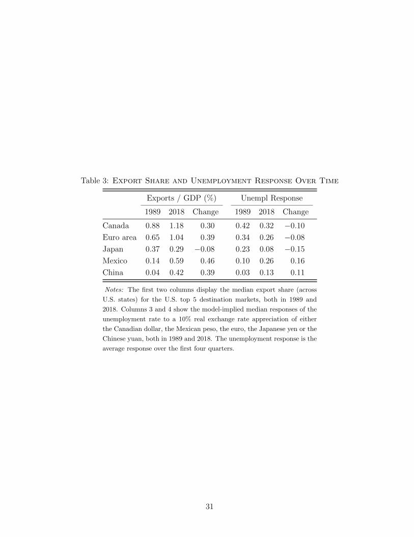
Table 3: Export Share and Unemployment Response Over Time

Exports / GDP (%) Unempl Response

1989 2018 Change 1989 2018 Change

Canada 0.88 1.18 0.30 0.42 0.32 −0.10

Euro area 0.65 1.04 0.39 0.34 0.26 −0.08

Japan 0.37 0.29 −0.08 0.23 0.08 −0.15

Mexico 0.14 0.59 0.46 0.10 0.26 0.16

China 0.04 0.42 0.39 0.03 0.13 0.11

Notes: The first two columns display the median export share (across

U.S. states) for the U.S. top 5 destination markets, both in 1989 and

2018. Columns 3 and 4 show the model-implied median responses of the

unemployment rate to a 10% real exchange rate appreciation of either

the Canadian dollar, the Mexican peso, the euro, the Japanese yen or the

Chinese yuan, both in 1989 and 2018. The unemployment response is the

average response over the first four quarters.

31

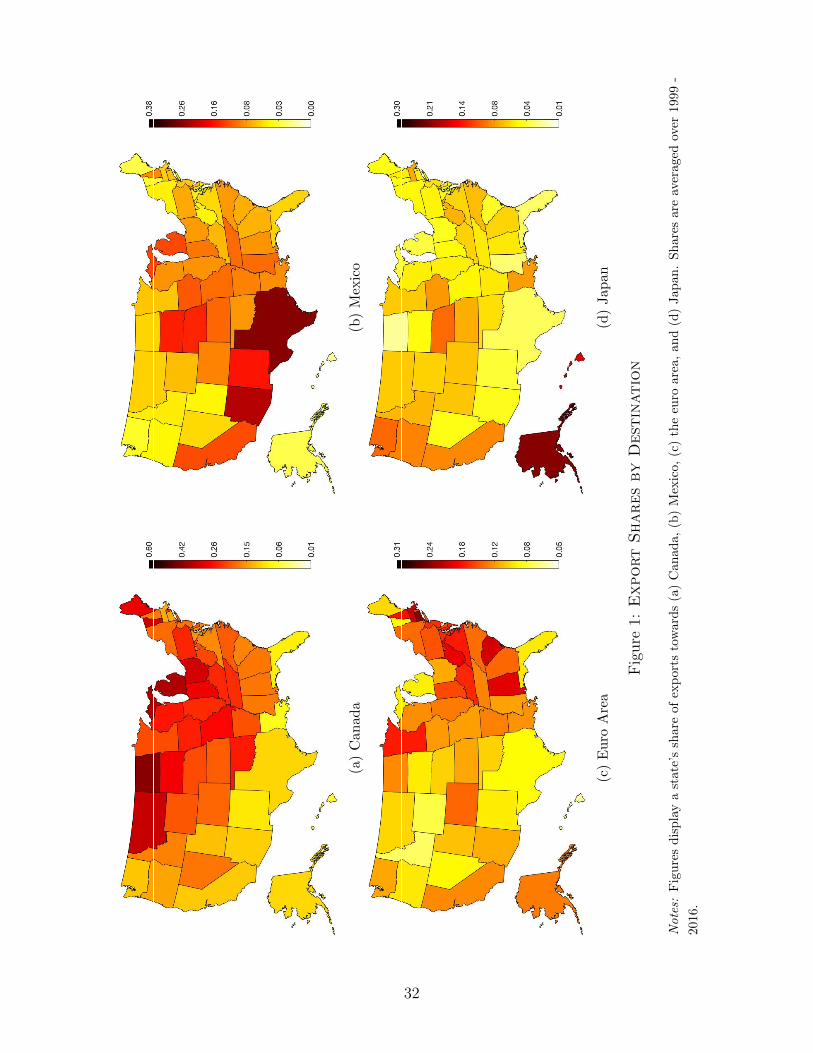
(a)

Can

ada

(b)

Mex

ico

(c)

Eu

roA

rea

(d)

Jap

an

Fig

ure

1:ExportSharesbyDest

ination

Notes:

Fig

ure

sd

isp

lay

ast

ate

’ssh

are

ofex

por

tsto

war

ds

(a)

Can

ada,

(b)

Mex

ico,

(c)

the

euro

area

,an

d(d

)Jap

an.

Sh

ares

are

aver

aged

over

1999

-

2016

.

32

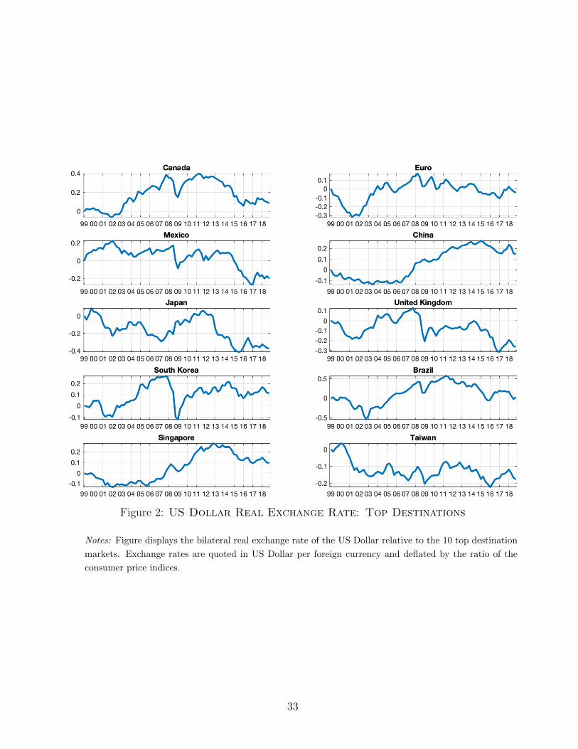
Figure 2: US Dollar Real Exchange Rate: Top Destinations

Notes: Figure displays the bilateral real exchange rate of the US Dollar relative to the 10 top destination

markets. Exchange rates are quoted in US Dollar per foreign currency and deflated by the ratio of the

consumer price indices.

33

Fig

ure

3:GrowthRatesoftheRealEffectiveExchangeRateAcross

U.S.States

Notes:

Fig

ure

dis

pla

ys

year

-to-y

ear

grow

thra

tes

ofth

ere

aleff

ecti

ve

exch

ange

rate

acro

ssst

ates

bet

wee

n20

01an

d20

18.

For

any

poin

tin

tim

et,

the

grow

thra

teb

etw

eent−

4an

dt

isd

isp

layed

.E

ffec

tive

exch

ange

rate

sar

eca

lcu

late

db

ased

onav

erag

eex

por

tsh

ares

over

the

last

fou

rqu

art

ers.

Exp

ort

dat

ast

art

sin

199

9q1,

soth

ateff

ecti

veex

chan

gera

tes

can

only

be

calc

ula

ted

star

tin

gin

2000

q1

and

annu

algr

owth

rate

sst

art

in2001q1.

Th

eth

ick

bla

ckli

ne

isth

egr

owth

rate

for

the

med

ian

stat

e,th

eh

eavy-s

had

edar

eais

the

inte

rqu

arti

lera

nge

,th

eli

ght-

shad

edar

eais

the

inte

rdec

ile

ran

gean

dth

eth

inb

lue

lin

esd

isp

lay

the

min

imu

man

dm

axim

um

grow

thra

tes

obse

rved

acro

ssU

.S.

stat

es.

34

(a)

Rea

lE

xch

ange

Rat

e(b

)E

xp

orts

and

Imp

orts

(c)

Un

emp

loym

ent

Rate

(d)

Sta

teG

DP

(e)

Hou

rsw

orke

d(f

)N

etm

igra

tion

Fig

ure

4:EmpiricalIm

pulse

Resp

onse

to

aRealEffectiveExchangeRateDepreciation

Notes:

Fig

ure

dis

pla

ys

the

loca

lp

roje

ctio

nof

(a)

the

real

effec

tive

exch

ange

rate

,(b

)n

omin

alex

por

tsan

dim

por

ts(e

xp

ress

edin

per

cent

of

state

’s

GD

P),

(c)

the

un

emp

loym

ent

rate

,(d

)st

ate

GD

P,

(e)

hou

rsw

orke

dan

d(f

)cu

mu

lati

ven

etim

mig

rati

onto

a1%

dep

reci

atio

nof

the

real

effec

tive

exch

ange

rate

bas

edon

regr

essi

on(2

.3).

Th

ed

efin

itio

nof

the

(exp

ort)

effec

tive

exch

ange

rate

cove

rsth

eU

.S.

mar

ket,

incl

ud

ing

the

state

itse

lf.

Sta

te

GD

Pis

real

,to

tal

GD

Pat

the

stat

ele

vel.

Ban

ds

are

90p

erce

nt

con

fid

ence

inte

rval

s.

35

(a)

Dat

a(b

)M

od

el

Fig

ure

5:UnemploymentRateResp

onse

to

aDepreciationoftheU.S.dollarand

ExportShares

Notes:

Pan

el(a

)d

isp

lays

the

esti

mat

edre

spon

seof

the

un

emp

loym

ent

aver

aged

over

the

firs

tfo

ur

qu

arte

rsfo

ran

app

reci

atio

nof

the

U.S

.d

oll

ar

rela

tive

toon

eof

the

five

top

exp

ort

mar

kets

asa

fun

ctio

nof

ast

ate’

sex

por

tsto

that

mar

ket

(nor

mal

ized

by

ast

ate’

sG

DP

).E

ach

dot

rep

rese

nts

anes

tim

ated

regr

essi

onco

effici

ent,

1 4

∑ 3 h=0βh,js,n

,an

dth

eve

rtic

alli

nes

are

stan

dar

dd

evia

tion

s,1 4

∑ 3 h=0

( βh,js,n±std( β

h,js,n

)) .P

anel

(b)

dis

pla

ys

the

coeffi

cien

tsfr

omth

esi

mu

late

dre

spon

sein

the

mod

el.

36

(a) Exports (b) Unemployment Rate

(c) State GDP (d) Hours Worked

Figure 6: Response to an Exchange Rate Depreciation Over the Business Cycle

Notes: Figure displays the local projection of (a) nominal exports (expressed in percent of state’s GDP),

(b) the unemployment rate, (c) state GDP, (d) hours worked to a 1% depreciation of the real effective

exchange rate based on regression (2.5). The definition of the (export) effective exchange rate covers

the U.S. market, including the state itself. State GDP is real, total GDP at the state level. Bands are

1-standard error-deviation bounds. Slack is identified as time periods where a state’s unemployment rate

exceeds 6.5 percent.

37

(a)

Un

emp

loym

ent

Rat

e(b

)G

DP

Fig

ure

7:Im

pulse

Resp

onse

to

aRealEffectiveExchangeRateDepreciation

Notes:

Fig

ure

dis

pla

ys

the

loca

lp

roje

ctio

nof

(a)

the

un

emp

loym

ent

rate

and

(b)

stat

eG

DP

toa

1p

erce

nt

app

reci

atio

nof

the

effec

tive

exch

an

ge

rate

bas

edon

regre

ssio

n(2

.3).

Th

ed

efin

itio

nof

the

(exp

ort)

effec

tive

exch

ange

rate

cove

rsth

eU

.S.

mar

ket,

incl

udin

gth

est

ate

itse

lf.

Both

the

resp

onse

inth

eac

tual

dat

aan

dth

esi

mu

late

db

ench

mar

km

od

elar

ed

isp

layed

.B

and

sar

e90

per

cent

con

fid

ence

inte

rval

s.

38

(a) No Migration (b) No Interstate Trade

(c) Financial Autarky

Figure 8: Model Response of Unemployment to an Exchange Rate Depreciation

Notes: See Figure 7. Only impulse responses based on the benchmark model and the various counterfac-

tuals are displayed.

39

(a) Exports to China as Share of GDP

(b) Unemployment Response to a 25% China Tariff

Figure 9: Export Exposure to China and Effects of Tariff on Unemployment.

Notes: Figure (a) displays exports to China as a share of state GDP (in percent, as of 2018). Figure (b)

displays the model-implied change in the unemployment rate in response to a 25 percent tariff imposed

by China on U.S. exports averaged over the first year.

40