Embed Size (px)
Citation preview

EPA United States Environmental Protection Agency
Regional Benefits Analysis for the Final Section 316(b) Phase III Existing Facilities Rule June 2006
U.S. Environmental Protection Agency Office of Water (4303T)
1200 Pennsylvania Avenue, NW Washington, DC 20460
EPA-821-R-04-007

Section 316(b) Final Rule: Phase III – Regional Benefits Assessment Table of Contents
TOC i
Table of Contents Introduction Part A: Evaluation Methods Chapter A1: Methods Used to Evaluate I&E A1-1 Objectives of EPA’s Evaluation of I&E Data A1-2 Rationale for EPA’s Approach to Evaluating I&E of Harvested Species A1-3 Source Data A1-4 Methods for Evaluating I&E A1-5 Extrapolation of I&E Rates Chapter A2: Uncertainty A2-1 Types of Uncertainty A2-2 Monte Carlo Analysis as a Tool for Quantifying Uncertainty A2-3 EPA’s Uncertainty Analysis of Yield Estimates A2-4 Conclusions Chapter A3: Economic Benefit Categories and Valuation A3-1 Economic Benefit Categories Applicable to the Regulatory Analysis Options for Phase III Facilities A3-2 Direct Use Benefits A3-3 Indirect Use Benefits A3-4 Non-Use Benefits A3-5 Summary of Benefit Categories A3-6 Causality: Linking the Regulatory Analysis Options for Phase III Existing Facilities to Beneficial
Outcomes A3-7 Conclusions Chapter A4: Methods for Estimating Commercial Fishing Benefits A4-1 Overview of the Commercial Fisheries Sector A4-2 The Role of Fishing Regulations and Regulatory Participants A4-3 Overview of U.S. Commercial Fisheries A4-4 Prices, Quantities, Gross Revenue, and Economic Surplus A4-5 Economic Surplus A4-6 Surplus Estimation When There is No Anticipated Change in Price A4-7 Surplus Estimation Under Scenarios in Which Price May Change A4-8 Estimating Post-Harvest Economic Surplus in Tiered Markets A4-9 Nonmonetary Benefits of Commercial Fishing A4-10 Estimating Producer Surplus A4-11 Methods Used to Estimate Commercial Fishery Benefits from Reduced I&E; Summary A4-12 Limitations and Uncertainties Chapter A5: Recreational Fishing Benefits Methodology A5-1 Literature Review Procedure and Organization A5-2 Description of Studies A5-3 Meta-Analysis of Recreational Fishing Studies: Regression Model A5-4 Application of the Meta-Analysis Results to the Analysis of Recreational Benefits of the
Section 316(b) Regulatory Analysis Options for Phase III Facilities A5-5 Limitations and Uncertainties

Section 316(b) Final Rule: Phase III – Regional Benefits Assessment Table of Contents
TOC ii
Chapter A6: Qualitative Assessment of Non-Use Benefits A6-1 Public Policy Significance of Ecological Improvements from the Regulatory Analysis Options for
Phase III Facilities Chapter A7: Entrainment Survival A7-1 The Causes of Entrainment Mortality A7-2 Factors Affecting the Determination of Entrainment Survival A7-3 Detailed Analysis of Entrainment Survival Studies Reviewed A7-4 Discussion of Review Criteria A7-5 Applicability of Entrainment Survival Studies to Other Facilities A7-6 Conclusions Chapter A8: Discounting Benefits A8-1 Timing of Benefits A8-2 Discounting and Annualization Chapter A9: Threatened & Endangered Species Analysis Methods A9-1 Listed Species Background A9-2 Benefit Categories Applicable for Impacts on T&E Species A9-3 Methods Available for Estimating the Economic Value Associated with I&E of T&E Species A9-4 Issues in Estimating and Valuing Environmental Impacts from I&E on T&E Species Part B: California Chapter B1: Background B1-1 Facility Characteristics Chapter B2: Evaluation of Impingement and Entrainment in California B2-1 I&E Species/Species Groups Evaluated B2-2 I&E Data Evaluated B2-3 EPA’s Estimate of Current I&E at Phase III Facilities in California Expressed as Age-1 Equivalents and
Foregone Yield B2-4 Reductions in I&E at Phase III Facilities in the California Region Under Alternative Options B2-5 Assumptions Used in Calculating Recreational and Commercial Losses Chapter B3: Commercial Fishing Benefits B3-1 Baseline Commercial Losses B3-2 Expected Benefits Under Regulatory Analysis Options Chapter B4: Recreational Use Benefits B4-1 Benefit Transfer Approach Based on Meta-Analysis B4-2 Limitations and Uncertainty Chapter B5: Federally Listed T&E Species in the California Region Appendix B1: Life History Parameter Values Used to Evaluate I&E in the California Region Appendix B2: Reductions in I&E Under Supplemental Policy Options Appendix B3: Commercial Fishing Benefits Under Supplemental Policy Options Appendix B4: Recreational Use Benefits Under Supplemental Policy Options
Section 316(b) Final Rule: Phase III – Regional Benefits Assessment Table of Contents
TOC iii
Part C: North Atlantic Chapter C1: Background C1-1 Facility Characteristics Chapter C2: Evaluation of Impingement and Entrainment in the North Atlantic Region C2-1 I&E Species/Species Groups Evaluated C2-2 I&E Data Evaluated C2-3 EPA’s Estimate of Current I&E at Phase III Facilities in the North Atlantic Region Expressed as
Age-1 Equivalents and Foregone Yield C2-4 Reductions in I&E at Phase III Facilities in the North Atlantic Region Under Alternative Options C2-5 Assumptions Used in Calculating Recreational and Commercial Losses Chapter C3: Commercial Fishing Benefits C3-1 Baseline Commercial Losses C3-2 Expected Benefits Under Regulatory Analysis Options Chapter C4: Recreational Use Benefits C4-1 Benefit Transfer Approach Based on Meta-Analysis C4-2 Limitations and Uncertainty Chapter C5: Federally Listed T&E Species in the North Atlantic Region Appendix C1: Life History Parameter Values Used to Evaluate I&E in the North Atlantic Region Appendix C2: Reductions in I&E Under Supplemental Policy Options Appendix C3: Commercial Fishing Benefits Under Supplemental Policy Options Appendix C4: Recreational Use Benefits Under Supplemental Policy Options Part D: Mid-Atlantic Region Chapter D1: Background D1-1 Facility Characteristics Chapter D2: Evaluation of Impingement and Entrainment in the Mid-Atlantic Region D2-1 I&E Species/Species Groups Evaluated D2-2 I&E Data Evaluated D2-3 EPA’s Estimate of Current I&E at Phase III Facilities in the Mid-Atlantic Region Expressed as
Age-1 Equivalents and Foregone Yield D2-4 Reductions in I&E at Phase III Facilities in the Mid-Atlantic Region Under Alternative Options D2-5 Assumptions Used in Calculating Recreational and Commercial Losses Chapter D3: Commercial Fishing Benefits D3-1 Baseline Commercial Losses D3-2 Expected Benefits Under Regulatory Analysis Options Chapter D4: Recreational Use Benefits D4-1 Benefit Transfer Approach Based on Meta-Analysis D4-2 Limitations and Uncertainty Chapter D5: Federally Listed T&E Species in the Mid-Atlantic Region

Section 316(b) Final Rule: Phase III – Regional Benefits Assessment Table of Contents
TOC iv
Appendix D1: Life History Parameter Values Used to Evaluate I&E in the Mid-Atlantic Region Appendix D2: Reductions in I&E Under Supplemental Policy Options Appendix D3: Commercial Fishing Benefits Under Supplemental Policy Options Appendix D4: Recreational Use Benefits Under Supplemental Policy Options Part E: Gulf of Mexico Chapter E1: Background E1-1 Facility Characteristics Chapter E2: Evaluation of Impingement and Entrainment in the Gulf of Mexico E2-1 I&E Species/Species Groups Evaluated E2-2 I&E Data Evaluated E2-3 EPA’s Estimate of Current I&E at Phase III Facilities in the Gulf Region Expressed as
Age-1 Equivalents and Foregone Yield E2-4 Reductions in I&E at Phase III Facilities in the Gulf of Mexico Region Under Alternative Options E2-5 Assumptions Used in Calculating Recreational and Commercial Losses Chapter E3: Commercial Fishing Benefits E3-1 Baseline Commercial Losses E3-2 Expected Benefits Under Regulatory Analysis Options Chapter E4: Recreational Use Benefits E4-1 Benefit Transfer Approach Based on Meta-Analysis E4-2 Limitations and Uncertainty Chapter E5: Federally Listed T&E Species in the Gulf of Mexico Region Appendix E1: Life History Parameter Values Used to Evaluate I&E in the Gulf of Mexico Region Appendix E2: Reductions in I&E Under Supplemental Policy Options Appendix E3: Commercial Fishing Benefits Under Supplemental Policy Options Appendix E4: Recreational Use Benefits Under Supplemental Policy Options Part F: The Great Lakes Chapter F1: Background F1-1 Facility Characteristics Chapter F2: Evaluation of Impingement and Entrainment in the Great Lakes Region F2-1 I&E Species/Species Groups Evaluated F2-2 I&E Data Evaluated F2-3 EPA’s Estimate of Current I&E at Phase III Facilities in the Great Lakes Region Expressed as
Age-1 Equivalents and Foregone Yield F2-4 Reductions in I&E at Phase III Facilities in the Great Lakes Region Under Alternative Options F2-5 Assumptions Used in Calculating Recreational and Commercial Losses Chapter F3: Commercial Fishing Benefits F3-1 Baseline Commercial Losses F3-2 Expected Benefits Under Regulatory Analysis Options

Section 316(b) Final Rule: Phase III – Regional Benefits Assessment Table of Contents
TOC v
Chapter F4: Recreational Use Benefits F4-1 Benefit Transfer Approach Based on Meta-Analysis F4-2 Limitations and Uncertainty Chapter F5: Federally Listed T&E Species in the Great Lakes Region Appendix F1: Life History Parameter Values Used to Evaluate I&E in the Great Lakes Region Appendix F2: Reductions in I&E Under Supplemental Policy Options Appendix F3: Commercial Fishing Benefits Under Supplemental Policy Options Appendix F4: Recreational Use Benefits Under Supplemental Policy Options Part G: The Inland Region Chapter G1: Background G1-1 Facility Characteristics Chapter G2: Evaluation of Impingement and Entrainment in the Inland Region G2-1 I&E Species/Species Groups Evaluated G2-2 I&E Data Evaluated G2-3 EPA’s Estimate of Current I&E at Phase III Facilities in the Inland Region Expressed as
Age-1 Equivalents and Foregone Yield G2-4 Reductions in I&E at Phase III Facilities in the Inland Region Under Alternative Options G2-5 Assumptions Used in Calculating Recreational and Commercial Losses Chapter G3: Commercial Fishing Benefits Chapter G4: Recreational Use Benefits G4-1 Benefit Transfer Approach Based on Meta-Analysis G4-2 Limitations and Uncertainty Chapter G5: Federally Listed T&E Species in the Inland Region Appendix G1: Life History Parameter Values Used to Evaluate I&E in the Inland Region Appendix G2: Reductions in I&E Under Supplemental Policy Options Appendix G3: Commercial Fishing Benefits Under Supplemental Policy Options Appendix G4: Recreational Use Benefits Under Supplemental Policy Options Part H: South Atlantic Chapter H1: Background H1-1 Facility Characteristics Chapter H2: Evaluation of Impingement and Entrainment in the South Atlantic Region H2-1 I&E Species/Species Groups Evaluated H2-2 I&E Data Evaluated H2-3 EPA’s Estimate of Current I&E at Phase III Facilities in the South Atlantic Region Expressed as Age-1
Equivalents and Foregone Yield H2-4 Reductions in I&E at Phase III Facilities in the South Atlantic Region H2-5 Assumptions Used in Calculating Recreational and Commercial Losses

Section 316(b) Final Rule: Phase III – Regional Benefits Assessment Table of Contents
TOC vi
Chapter H3: Commercial Fishing Benefits H3-1 Baseline Commercial Losses H3-2 Expected Benefits Under Regulatory Analysis Options Chapter H4: Recreational Use Benefits H4-1 Benefit Transfer Approach Based on Meta-Analysis H4-2 Limitations and Uncertainty Chapter H5: Federally Listed T&E Species in the South Atlantic Region Appendix H1: Life History Parameter Values Used to Evaluate I&E in the South Atlantic Region Appendix H2: Reductions in I&E Under Supplemental Policy Options Appendix H3: Commercial Fishing Benefits Under Supplemental Policy Options Appendix H4: Recreational Use Benefits Under Supplemental Policy Options Part I: National Benefits Chapter I1: National Benefits I1-1 Calculating National Losses and Benefits I1-2 Summary of Baseline Losses and Expected Reductions in I&E I1-3 Time Profile of Benefits I1-4 National Benefits from Eliminating and Reducing I&E Losses Appendix I1: National Benefits Under Supplemental Policy Options References
Section 316(b) Final Rule: Phase III – Regional Benefits Assessment Introduction
1-1
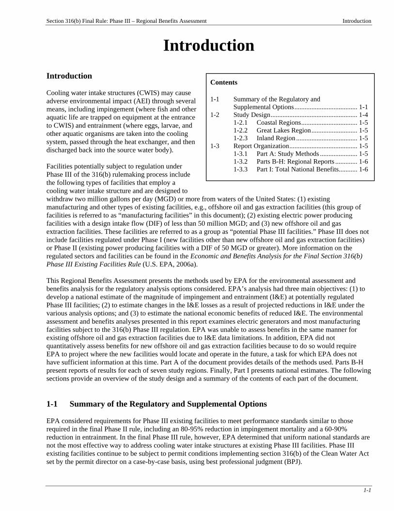
Introduction Introduction Cooling water intake structures (CWIS) may cause adverse environmental impact (AEI) through several means, including impingement (where fish and other aquatic life are trapped on equipment at the entrance to CWIS) and entrainment (where eggs, larvae, and other aquatic organisms are taken into the cooling system, passed through the heat exchanger, and then discharged back into the source water body). Facilities potentially subject to regulation under Phase III of the 316(b) rulemaking process include the following types of facilities that employ a cooling water intake structure and are designed to withdraw two million gallons per day (MGD) or more from waters of the United States: (1) existing manufacturing and other types of existing facilities, e.g., offshore oil and gas extraction facilities (this group of facilities is referred to as “manufacturing facilities” in this document); (2) existing electric power producing facilities with a design intake flow (DIF) of less than 50 million MGD; and (3) new offshore oil and gas extraction facilities. These facilities are referred to as a group as “potential Phase III facilities.” Phase III does not include facilities regulated under Phase I (new facilities other than new offshore oil and gas extraction facilities) or Phase II (existing power producing facilities with a DIF of 50 MGD or greater). More information on the regulated sectors and facilities can be found in the Economic and Benefits Analysis for the Final Section 316(b) Phase III Existing Facilities Rule (U.S. EPA, 2006a). This Regional Benefits Assessment presents the methods used by EPA for the environmental assessment and benefits analysis for the regulatory analysis options considered. EPA’s analysis had three main objectives: (1) to develop a national estimate of the magnitude of impingement and entrainment (I&E) at potentially regulated Phase III facilities; (2) to estimate changes in the I&E losses as a result of projected reductions in I&E under the various analysis options; and (3) to estimate the national economic benefits of reduced I&E. The environmental assessment and benefits analyses presented in this report examines electric generators and most manufacturing facilities subject to the 316(b) Phase III regulation. EPA was unable to assess benefits in the same manner for existing offshore oil and gas extraction facilities due to I&E data limitations. In addition, EPA did not quantitatively assess benefits for new offshore oil and gas extraction facilities because to do so would require EPA to project where the new facilities would locate and operate in the future, a task for which EPA does not have sufficient information at this time. Part A of the document provides details of the methods used. Parts B-H present reports of results for each of seven study regions. Finally, Part I presents national estimates. The following sections provide an overview of the study design and a summary of the contents of each part of the document. 1-1 Summary of the Regulatory and Supplemental Options EPA considered requirements for Phase III existing facilities to meet performance standards similar to those required in the final Phase II rule, including an 80-95% reduction in impingement mortality and a 60-90% reduction in entrainment. In the final Phase III rule, however, EPA determined that uniform national standards are not the most effective way to address cooling water intake structures at existing Phase III facilities. Phase III existing facilities continue to be subject to permit conditions implementing section 316(b) of the Clean Water Act set by the permit director on a case-by-case basis, using best professional judgment (BPJ).
Contents 1-1 Summary of the Regulatory and Supplemental Options..................................... 1-1 1-2 Study Design................................................... 1-4 1-2.1 Coastal Regions................................. 1-5 1-2.2 Great Lakes Region........................... 1-5 1-2.3 Inland Region .................................... 1-5 1-3 Report Organization........................................ 1-5 1-3.1 Part A: Study Methods ...................... 1-5 1-3.2 Parts B-H: Regional Reports ............. 1-6 1-3.3 Part I: Total National Benefits........... 1-6

Section 316(b) Final Rule: Phase III – Regional Benefits Assessment Introduction
1-2
The performance standards presented at proposal were intended to reflect the best technology available for minimizing AEIs determined on a national categorical basis. The type of performance standard applicable to a particular facility (i.e., reductions in impingement only or I&E) would have varied based on several factors, including the facility’s location (i.e., source waterbody) and the proportion of the waterbody withdrawn. Impingement reductions were required at all facilities subject to the performance standards. Entrainment reductions are required at facilities (1) located on an estuary, tidal river, ocean, or one of the Great Lakes; or (2) located on a freshwater river and withdrawing greater than 5% of the mean annual flow of the waterbody. At proposal, facilities located on lakes or reservoirs may not disrupt the thermal stratification of the waterbody, except in cases where the disruption is beneficial to the management of fisheries. EPA proposed three possible options for defining which existing manufacturing facilities would be subject to uniform national requirements, based on DIF threshold and source waterbody type: the facility has a total DIF of 50 MGD or more, and withdraws from any waterbody; the facility has a total DIF of 200 MGD or more, and withdraws from any waterbody; or the facility has a total DIF of 100 MGD or more and withdraws water specifically from an ocean, estuary, tidal river, or one of the Great Lakes. These are options 5, 9, and 8, respectively, in Table 1-1 below. In addition, EPA considered a number of options (specifically options 2, 3, 4, and 7 below) that establish different performance standards for certain groups or subcategories of Phase III existing facilities. Under these options, EPA would have applied the proposed performance standards and compliance alternatives (i.e., the Phase II requirements) to the higher threshold facilities, apply the less-stringent requirements as specified below to the middle flow threshold category, and would apply BPJ below the lower threshold. The regulatory options as well as other options considered are described in detail below: Option 1: Facilities with a DIF of 20 MGD or greater would be subject to the performance standards discussed above. Under this option, section 316(b) permit conditions for Phase III facilities with a DIF of less than 20 MGD would be established on a case-by-case, BPJ, basis. Option 2: Facilities with a DIF of 50 MGD or greater, as well as facilities with a DIF between 20 and 50 MGD (20 MGD inclusive), when located on estuaries, oceans, or the Great Lakes would be subject to the performance standards. Facilities with a DIF between 20 and 50 MGD (20 MGD inclusive) that withdraw from freshwater rivers and lakes would have to meet the performance standards for impingement mortality only and not for entrainment. Under this option, section 316(b) requirements for Phase III facilities with a DIF of less than 20 MGD would be established on a case-by-case, BPJ, basis. Option 3: Facilities with a DIF of 50 MGD or greater would be subject to the performance standards. Facilities with a DIF between 20 and 50 MGD (20 MGD inclusive) would have to meet the performance standards for impingement mortality only and not for entrainment. Under this option, section 316(b) requirements for Phase III facilities with a DIF of less than 20 MGD would be established on a case-by-case, BPJ, basis. Option 4: Facilities with a DIF of 50 MGD or greater, as well as facilities with a DIF between 20 and 50 MGD (20 MGD inclusive), when located on estuaries, oceans, or the Great Lakes would be subject to the performance standards. Facilities that withdraw from freshwater rivers and lakes and all facilities with a DIF of less than 20 MGD would have requirements established on a case-by-case, BPJ, basis. Option 5: Facilities with a DIF of 50 MGD or greater would be subject to the performance standards. Under this option, section 316(b) requirements for Phase III facilities with a DIF of less than 50 MGD would be established on a case-by-case, BPJ, basis. Option 6: Facilities with a DIF of greater than 2 MGD would be subject to the performance standards. Under this option, section 316(b) requirements for Phase III facilities with a DIF of 2 MGD or less would be established on a case-by-case, BPJ, basis.
Section 316(b) Final Rule: Phase III – Regional Benefits Assessment Introduction
1-3
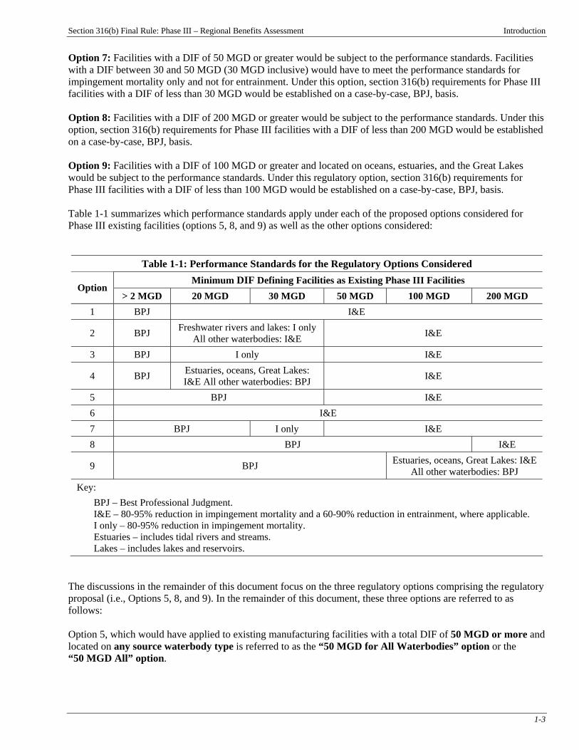
Option 7: Facilities with a DIF of 50 MGD or greater would be subject to the performance standards. Facilities with a DIF between 30 and 50 MGD (30 MGD inclusive) would have to meet the performance standards for impingement mortality only and not for entrainment. Under this option, section 316(b) requirements for Phase III facilities with a DIF of less than 30 MGD would be established on a case-by-case, BPJ, basis. Option 8: Facilities with a DIF of 200 MGD or greater would be subject to the performance standards. Under this option, section 316(b) requirements for Phase III facilities with a DIF of less than 200 MGD would be established on a case-by-case, BPJ, basis. Option 9: Facilities with a DIF of 100 MGD or greater and located on oceans, estuaries, and the Great Lakes would be subject to the performance standards. Under this regulatory option, section 316(b) requirements for Phase III facilities with a DIF of less than 100 MGD would be established on a case-by-case, BPJ, basis. Table 1-1 summarizes which performance standards apply under each of the proposed options considered for Phase III existing facilities (options 5, 8, and 9) as well as the other options considered:
Table 1-1: Performance Standards for the Regulatory Options Considered Minimum DIF Defining Facilities as Existing Phase III Facilities
Option > 2 MGD 20 MGD 30 MGD 50 MGD 100 MGD 200 MGD
1 BPJ I&E
2 BPJ Freshwater rivers and lakes: I onlyAll other waterbodies: I&E I&E
3 BPJ I only I&E
4 BPJ Estuaries, oceans, Great Lakes: I&E All other waterbodies: BPJ I&E
5 BPJ I&E 6 I&E 7 BPJ I only I&E 8 BPJ I&E
9 BPJ Estuaries, oceans, Great Lakes: I&EAll other waterbodies: BPJ
Key: BPJ – Best Professional Judgment. I&E – 80-95% reduction in impingement mortality and a 60-90% reduction in entrainment, where applicable. I only – 80-95% reduction in impingement mortality. Estuaries – includes tidal rivers and streams. Lakes – includes lakes and reservoirs.
The discussions in the remainder of this document focus on the three regulatory options comprising the regulatory proposal (i.e., Options 5, 8, and 9). In the remainder of this document, these three options are referred to as follows: Option 5, which would have applied to existing manufacturing facilities with a total DIF of 50 MGD or more and located on any source waterbody type is referred to as the “50 MGD for All Waterbodies” option or the “50 MGD All” option.

Section 316(b) Final Rule: Phase III – Regional Benefits Assessment Introduction
1-4
Option 8, which would have applied to existing manufacturing facilities with a total DIF of 200 MGD or more and located on any source waterbody type is referred to as the “200 MGD for All Waterbodies” option or the “200 MGD All” option. Option 9, which would have applied to existing manufacturing facilities with a total DIF of 100 MGD or more and located on certain source waterbody types (i.e., an ocean estuary, tidal river/stream, or one of the Great Lakes) is referred to as the “100 MGD for Certain Waterbodies” option or the “100 MGD CWB” option. In addition to these three regulatory analysis options, this document also presents information on the other options that EPA analyzed in development of the Phase III proposal and the final regulation (i.e., Options 2, 3, 4, and 7, also referred to as the “supplemental options”). The information for the supplemental options is presented in appendices to the relevant chapters in this report. 1-2 Study Design EPA’s analysis of the regulation examined cooling water intake structure impacts and regulatory benefits at the regional scale, and then combined regional results to develop national estimates. EPA grouped facilities into regions for its analysis based on (1) the locations of facilities potentially subject to regulation in Phase III, (2) similarities among the aquatic species affected by these facilities, and (3) characteristics of commercial and recreational fishing activities in the area. Table 1-2 lists the number of potentially regulated facilities in each study region and the number of facilities with technology requirements under each of the regulatory analysis options, weighted using statistical weights from EPA’s survey of the industry. The seven regions and the waterbody types within each region are described below. Maps showing the facilities in each region are provided in the introductory chapter of each regional report (Parts B-H of this document).
Table 1-2: Number of Existing Phase III Facilities by Region and Option # of Facilities Subject to National Technology Requirements
(weighted)
Region
# of Potentially Regulated Existing Phase III Facilities
(weighted)a 50 MGD All 200 MGD All 100 MGD CWB Californiab 9 1 0 0 North Atlantic 5 4 1 3 Mid-Atlantic 15 3 2 2 South Atlantic 4 0 0 0 Gulf of Mexico 11 7 3 7 Great Lakes 45 18 7 10 Inland 540 78 13 0 National totalb,c 629 111 27 22 a Potentially regulated existing Phase III facilities include electric generators with CWIS that withdraw more than 2 MGD but less than 50 MGD and manufacturers with CWIS that withdraw more than 2 MGD and use at least 25% of the water for cooling purposes. b Numbers may not sum to totals due to independent rounding. c Eighty potentially regulated facilities determined to be baseline closures are excluded from this analysis.

Section 316(b) Final Rule: Phase III – Regional Benefits Assessment Introduction
1-5
1-2.1 Coastal Regions Coastal regions include estuary/tidal river and ocean facilities in five of the NOAA Fisheries regions. The North Atlantic region encompasses Maine, New Hampshire, Massachusetts, Connecticut, and Rhode Island. The Mid-Atlantic region includes New York, New Jersey, Maryland, the District of Columbia, Delaware, and Virginia. The Gulf of Mexico region includes Texas, Louisiana, Mississippi, Alabama, and the west coast of Florida. The California region includes all estuary/tidal river and ocean facilities in California, plus one facility in Hawaii. Although the Hawaii facility was considered in estimating baseline I&E in the California region, it is not subject to any of the options described in Table 1-2. Therefore no benefits are anticipated for this facility. The South Atlantic region includes North Carolina, South Carolina, Georgia, and the east coast of Florida. In the South Atlantic, all known in-scope facilities have DIFs that are less then 50 MGD, and therefore none are subject to the options described in Table 1-2. EPA’s survey did not locate any Phase III facilities within the Alaska NOAA Fisheries region. Although one Phase III facility is located in the Pacific Northwest Fisheries region, this facility is projected to close under the baseline scenario. Therefore, EPA did not include analysis of these two regions in this assessment. 1-2.2 Great Lakes Region The Great Lakes region includes all potentially regulated Phase III facilities that withdraw water from Lake Ontario, Lake Erie, Lake Huron (including Lake St. Clair), Lake Michigan, and Lake Superior, and the connecting channels (Saint Mary’s River, Saint Clair River, Detroit River, Niagara River, and Saint Lawrence River to the Canadian border). This region definition is based on the definition provided in Section 118(a)(3)(B) of the Clean Water Act. 1-2.3 Inland Region The Inland region includes all facilities located on freshwater rivers or streams and lakes or reservoirs, in all states, with the exception of facilities located in the Great Lakes region. 1-3 Report Organization 1-3.1 Part A: Study Methods 1-3.1.1 Evaluation of I&E Chapter A1 of Part A of this Regional Benefits Assessment describes the methods used to evaluate facility I&E data. Chapter A2 discusses uncertainties in the analysis. To obtain regional I&E estimates, EPA extrapolated loss rates from those facilities for which I&E data is available, referred to in this document as model facilities, to all Phase III facilities within the same region. These results were then summed to develop national estimates. EPA used I&E data from Phase II facilities to supplement the limited data available for Phase III facilities. 1-3.1.2 Economic Benefits Chapters A3-A6 and A8-A9 of Part A of this document describe the methods that EPA used for its analysis of the economic benefits of the section 316(b) rule for Phase III facilities. As discussed in Chapter A3, EPA considered the following benefit categories: recreational fishing benefits, commercial fishing benefits, and non-use benefits. The analysis of use benefits included benefits from improved commercial fishery yields and benefits to recreational anglers from improved fishing opportunities. Chapters A4 and A5 provide details on the methods used for these analyses. Chapter A6 presents qualitative assessment of ecological non-use benefits of the regulation. Non-use benefits included benefits from reduced I&E of forage species, and the non-landed portion of commercial and recreational species. Chapter A8 discusses discounting of recreational and commercial benefits. Methods for estimating benefits to threatened and endangered species are described in Chapter A9.

Section 316(b) Final Rule: Phase III – Regional Benefits Assessment Introduction
1-6
1-3.2 Parts B-H: Regional Reports Parts B-H of this Regional Benefits Assessment are reports of results for each study region. Chapter 1 of each report provides background information on the facilities in the region and a map showing facility locations. Chapter 2 provides I&E estimates. Benefits estimates are presented in Chapters 3 and 4. Chapter 3 presents estimates of commercial fishing benefits, and Chapter 4 presents recreational fishing benefits. Chapter 5 presents information on threatened and endangered species in each region. Appendix 1 of each regional report presents life history data and the data sources used in evaluations of I&E, and Appendix 2 presents results for supplementary policy options. Please see the TDD for additional information. 1-3.3 Part I: Total National Benefits Chapter I1 summarizes the results of the seven regional analyses and presents the total monetary value of national baseline losses and benefits for all section 316(b) Phase III manufacturing facilities (except oil and gas extraction facilities) and power generators.

Section 316(b) Final Rule: Phase III – Regional Benefits Assessment
Part A: Evaluation Methods
Section 316(b) Final Rule: Phase III – Regional Benefits Assessment, Part A: Evaluation Methods Chapter A1
A1-1
Chapter A1: Methods Used to Evaluate I&E Introduction
Chapter Contents A1-1 Objectives of EPA’s Evaluation of I&E Data .............................................................. A1-1 A1-2 Rationale for EPA’s Approach to Evaluating I&E of Harvested Species .......... A1-1 A1-2.1 Scope and Objectives of EPA’s Analysis of Harvested Species........ A1-2 A1-2.2 Data Availability and Uncertainties................................... A1-2 A1-2.3 Difficulties Distinguishing Causes of Population Changes.................... A1-3 A1-3 Source Data .................................................. A1-3 A1-3.1 Facility Impingement and
Entrainment Monitoring Data......... A1-3 A1-3.2 Species Groups ............................... A1-4 A1-3.3 Species Life History Parameters..... A1-4 A1-4 Methods for Evaluating I&E ........................ A1-5 A1-4.1 Modeling Age-1 Equivalents.......... A1-5 A1-4.2 Modeling Foregone Fishery Yield ............................................... A1-6 A1-4.3 Modeling Production Foregone ...... A1-9 A1-4.4 Evaluation of Forage Species Losses ........................................... A1-10 A1-5 Extrapolation of I&E Rates ........................ A1-11
This chapter describes the methods used by EPA to evaluate facility impingement and entrainment (I&E) data. Section A1-1 discusses the main objectives of EPA’s I&E evaluation. Section A1-2 describes EPA’s general approach to modeling fishery yield and the rationale for this approach. Section A1-3 describes the source data for EPA’s I&E evaluations. Section A1-4 presents details of the biological models used to evaluate I&E. Finally, section A1-5 discusses methods used to extrapolate I&E rates from facilities with I&E data to other facilities in the same region without data. A1-1 Objectives of EPA’s Evaluation of
I&E Data EPA’s evaluation of I&E data had four main objectives:
< to develop a national estimate of the magnitude of I&E;
< to standardize I&E rates using common biological metrics so that rates could be compared across species, years, facilities, and geographical regions;
< to estimate changes in these metrics as a result of projected reductions in I&E under the proposed regulatory options for the section 316(b) Phase III existing facilities rule; and
< to estimate the national economic benefits of reduced I&E. To accomplish these objectives, three loss metrics were derived from the facility I&E monitoring data available to EPA: (1) foregone age-1 equivalents, (2) foregone fishery yield, and (3) foregone biomass production. The methods used to calculate these metrics are described in section A1-4. Age-1 equivalent estimates were used to quantify losses of individuals in terms of a single life stage. Losses of commercial and recreational species were also expressed as foregone fishery yield. Estimates of production foregone were used to quantify the contribution of forage species to the yield of harvested species. The following section discusses EPA’s rationale for evaluating the I&E of harvested species in terms of foregone fishery yield. Foregone fishery yield is also referred to as harvest in the discussion below. A1-2 Rationale for EPA’s Approach to Evaluating I&E of Harvested Species EPA estimated I&E impacts to all fish and shellfish species for which data were available. EPA focused on harvested fish and shellfish species primarily because of the availability of economic methods for valuing these species (see Chapters A3-A6 and A8-A9 for a discussion of all of the economic methods used by EPA to estimate benefits of the proposed regulatory options for the section 316(b) rule for Phase III existing facilities). EPA’s
Section 316(b) Final Rule: Phase III – Regional Benefits Assessment, Part A: Evaluation Methods Chapter A1
A1-2
approach to estimating changes in harvest assumed that I&E losses result in a reduction in the number of harvestable adults in the years following the time at which individual fish are killed by I&E and that future reductions in I&E will lead to future increases in fish harvest. The approach does not require knowledge of population size or the total yield of a fishery; it only estimates the incremental yield that is foregone because of the number of deaths due to I&E. As discussed in detail in section A1-4.2, EPA’s foregone fishery yield analysis employed a specific application of the Thompson Bell model of fisheries yield (Ricker, 1975) to assess the effects of I&E on net fish harvest. This model is a relatively simple yield-per-recruit (YPR) model that provides estimates of yield that can be expected from a cohort of fish that is recruited to a fishery. The model requires estimates of size-at-age for particular species and stage-specific schedules of natural mortality (M) and fishing mortality (F). All of the key parameters used in the yield model (F, M, and size-at-age), were assumed to be constant for a given species regardless of changes in I&E rates. Because these parameters are held static for any particular fish stock, YPR is also a constant value. With this set of parameters fixed, the Thompson Bell model holds that an estimate of recruitment is directly proportional to an estimate of yield. EPA recognizes that the assumption that the key parameters are static is an important one that does not fully reflect the dynamic nature of fish populations. However, by focusing on a simple interpretation of each individual I&E death in terms of foregone yield, EPA concentrated on the simplest, most direct assessment of the potential economic value of eliminating that death. EPA believes that this approach was warranted given the (1) scope and objectives of its analysis of harvested species, (2) data available, and (3) difficulties in distinguishing the causes of population changes. Each of these factors is discussed in the following sections. A1-2.1 Scope and Objectives of EPA’s Analysis of Harvested Species The simplicity of EPA’s approach to modeling yield was consistent with the need to examine the dozens of harvested species that are vulnerable to I&E at the hundreds of facilities throughout the country that are in scope of the rule and the overall objective of developing regional- and national-scale estimates. This approach is not necessarily the best alternative for studies of single facilities for which site-specific details on local fish stocks and waterbody conditions might make possible the use of more complex assessment approaches (e.g., modeling of population or community level impacts). A1-2.2 Data Availability and Uncertainties Although EPA’s approach to modeling foregone fishery yield requires estimates of a large number of stage-specific growth and mortality parameters, the use of more complex fish population models would rely on an even larger set of parameters and would require numerous additional and stronger assumptions about the nature of stock dynamics that would be difficult to defend with available data. Additional uncertainties of population dynamics models include the relationship between stock size and recruitment, and how growth and mortality rates may change as a function of stock size and other factors. Obtaining this information for even one fish stock is time-consuming and resource intensive; obtaining this information for the many species subject to I&E nation-wide was not possible for EPA’s national benefits analysis because of the resources doing so would require. It is also important to note that information on stock status (e.g., spawning stock biomass, standardized catch-per-unit-effort, recruitment) is generally only available for harvested species, which represent a minor fraction of I&E losses. Even for harvested species, stock status is often poorly known. In fact, only 23% of U.S. managed fish stocks have been fully assessed (U.S. Ocean Commission, 2002). In addition to a lack of data, there are numerous issues and difficulties with defining the size and spatial extent of fish stocks. As a result, it is often unclear how I&E losses at particular cooling water intake structures can be related to specific stocks. For example, a recent study of Atlantic menhaden (Brevoortia tryannus), one of the major fish species subject to I&E along the Atlantic Coast of the U.S., indicated that juveniles in Delaware Bay result from both local and long distance recruitment (Light and Able, 2003). Thus, accounting only for influences

Section 316(b) Final Rule: Phase III – Regional Benefits Assessment, Part A: Evaluation Methods Chapter A1
A1-3
on local recruitment would be insufficient for understanding the relationship between recruitment and menhaden stock size. Another difficulty is that fisheries managers typically define fish stocks by reference to the geographic scope of the fishery responsible for landings. However, landings data are reported state by state, which is generally not a good way to delineate the true spatial extent of fish populations. These types of delineations create uncertainty in the definition of stocks for the purposes of modeling their population dynamics. A1-2.3 Difficulties Distinguishing Causes of Population Changes Another problem in developing and implementing more complex models of harvested species is that it is fundamentally difficult to demonstrate that any particular kind of stress causes a reduction in fish population size. All fish populations are under a variety of stresses that are difficult to quantify given the data currently available and that may interact in a non-additive manner. Fish populations are perpetually in flux for numerous reasons, so determining a baseline population size, then detecting a trend, and then determining if a trend is a significant deviation from an existing baseline or is simply an expected fluctuation around a stable equilibrium is problematic. Fish recruitment is a multidimensional process, and identifying and distinguishing the causes of variance in fish recruitment remains a fundamental problem in fisheries science, stock management, and impact assessment (Hilborn and Walters, 1992; Quinn and Deriso, 1999; Boreman, 2000). Resolving this issue was beyond the scope and objectives of EPA’s section 316(b) benefits analysis. A1-3 Source Data The inputs for EPA’s analyses included facility I&E monitoring data collected by facilities with cooling water intake structures and species life history characteristics from the scientific literature such as growth rates, natural mortality rates, and fishing mortality rates. A1-3.1 Facility Impingement and Entrainment Monitoring Data The general approach to I&E monitoring was similar at most facilities, but investigators used a wide variety of methods that were specific to the individual studies, e.g., location of sampling stations, sampling gear, sampling frequency, and enumeration techniques. Facilities generally monitored only fish and shellfish species and did not monitor I&E of other types of aquatic organisms. Some facilities monitored only a subset of all fish and shellfish species impinged and entrained. Impingement monitoring typically involves sampling impingement screens or catchment areas, counting the impinged fish, and extrapolating the count to an annual basis. Entrainment monitoring typically involves intercepting a small portion of the intake flow at a selected location in the facility, collecting fish by sieving the water sample through nets or other collection devices, counting the collected fish, and extrapolating the counts to an annual basis. EPA retained all information regarding species, life stage, and loss modality (I or E) as they were originally reported by the facilities, with the exception of some species aggregation that is described in section A1-3.2. Facility studies were excluded from EPA’s analysis if the information reported was not suitable for the models used by EPA, which require annual loss rates expressed on a species- and age-specific basis. Studies were also excluded if the study involved sampling at a limited portion of the facility, e.g., at only one of the several intakes, but did not supply sufficient information to conduct a reliable extrapolation from recorded losses to an estimate of total losses (e.g., flow rates at sampled intakes or a description of the reasoning behind the sampling design). In some cases, entrainment sampling was conducted only during the months that larvae are present at a particular facility (usually spring and summer), and in such cases EPA assumed that entrainment rates for these months were indicative of the total annual loss.
Section 316(b) Final Rule: Phase III – Regional Benefits Assessment, Part A: Evaluation Methods Chapter A1
A1-4
In most cases the size or life stage (i.e., age) of impinged fish are not reported. However, the EPA modeling procedure requires the age of the killed fish. Therefore, EPA assumed the age of impinged fish ranged from the juvenile stage to age 5, and divided the total impingement losses into age groups using proportions corresponding to the expected life table dictated by species-specific mortality schedules. EPA adjusted annualized loss rates at some facilities as needed to reflect the history of technological changes at the facility. The purpose of the adjustments was to interpret loss records in a way that best reflects the current conditions at each facility. For example, if a facility was known to have installed a protective technology subsequent to the time that I&E loss rates were recorded, EPA reduced the loss rates in an amount corresponding to the presumed effectiveness of the protective technology (see the Technical Development Document for the Final Section 316(b) Phase III Existing Facilities Rule). Loss rates recorded at each facility were expressed as an annual average rate, regardless of the number of years of sampling data available. The annual total among the facilities evaluated was then the subject of the detailed modeling procedure described in section A1-4. Once this analysis was completed, estimates of total losses, by region, were generated using the extrapolation procedures described in section A1-5. A1-3.2 Species Groups EPA organized species for which there were limited data into groups and then conducted detailed analyses of I&E rates for each species group. Species groups were based on similarities in life history characteristics and groupings for landings data used by the National Oceanic and Atmospheric Administration (NOAA) Fisheries office (formerly the National Marine Fisheries Service). An appendix to each regional report in Parts B-H of this document provides details on the species, species groups, and life history data that were used. A1-3.3 Species Life History Parameters The life history parameters used in EPA’s analysis of I&E data included species growth rates, the fraction of each age class vulnerable to harvest, fishing mortality rates, and natural (nonfishing) mortality rates. Each of these parameters was also stage-specific. For the purpose of this assessment, EPA uses the terms “age” and “stage” interchangeably. For fish age 1 and older, a stage corresponds directly to the age in years of the fish. For fish younger than age one, loss data for early life stages were assigned to one of three life stages (eggs, larvae, and juveniles). If the literature provided survival rates of a more detailed staging scheme (e.g., yolk-sac larvae or post-yolk-sac larvae), survival rates were combined to reflect survival for the entire larval life stage. EPA obtained life history parameters from facility reports, the fisheries literature, local fisheries experts, and publicly available fisheries databases (e.g., FishBase). To the extent feasible, EPA identified region-specific life history parameters. All I&E losses of a particular species or species group within a region were modeled with a single set of parameters. Detailed citations are provided in the life history appendix accompanying each regional report (Parts B-H of the Regional Benefits Assessment). For most species in most regions a reasonable set of life history parameter values was identified. However, in a few cases where no information on survival rates was available for individual life stages, EPA deduced survival rates for an equilibrium population based on records of lifetime fecundity using the relationship presented in Goodyear (1978) and below in Equation 1:
Section 316(b) Final Rule: Phase III – Regional Benefits Assessment, Part A: Evaluation Methods Chapter A1
A1-5
SBBBeqBBB = 2/fa where: SBBBeqBBB = the probability of survival from egg to the expected age of spawning
females fa = the expected lifetime total egg production
(Equation 1)
Published fishing mortality rates (F) were assumed to reflect combined mortality due to both commercial and recreational fishing. Basic fishery science relationships (Ricker, 1975) among mortality and survival rates were assumed, such as:
Z = M + F where: Z = the total instantaneous mortality rate M = natural (nonfishing) instantaneous mortality rate F = fishing instantaneous mortality rate and S = ePPP
(-Z)PPP
where: S = the survival rate as a fraction
(Equation 2)
(Equation 3)
A1-4 Methods for Evaluating I&E The methods used to express I&E losses in units suitable for economic valuation are outlined in Figure A1-1 and described in detail in the following sections. A1-4.1 Modeling Age-1 Equivalents The Equivalent Adult Model (EAM) is a method for expressing I&E losses as an equivalent number of individuals at some other life stage, referred to as the age of equivalency (Horst, 1975; Goodyear, 1978; Dixon, 1999). The age of equivalency can be any life stage of interest. The method provides a convenient means of converting losses of fish eggs and larvae into units of individual fish and provides a standard metric for comparing losses among species, years, and regions. For the Regional Benefits Assessment, EPA expressed I&E losses at all life stages as an equivalent number of age-1 year individuals. The EAM calculation for each species requires life-stage-specific I&E counts and life-stage-specific mortality rates from the life stage of I&E to the life stage of equivalence (age 1 year, for this assessment). The cumulative survival rate from age at impingement or entrainment until age 1 is the product of all stage-specific survival rates to age 1. For impinged fish that are older than age 1, age-1 equivalents are calculated by modifying the basic calculation to inflate the loss rates in inverse proportion to survival rates. In the case of entrainment, the basic calculation is:
Section 316(b) Final Rule: Phase III – Regional Benefits Assessment, Part A: Evaluation Methods Chapter A1
A1-6
ij
jijj SSS ∏
+==
max
1
*1,
where: SBBB j,1 BBB = cumulative survival from stage j until age 1 SPPP
*PBPBPBjBBB = 2SBBBjBBBePPP
-log(1+Sj)PPP = adjusted SBBBjBBB
jBBBmaxBBB = the stage immediately prior to age 1 SBBBi BBB = survival fraction from stage i to stage i + 1
(Equation 4)
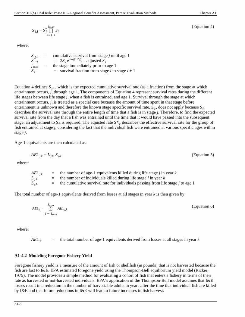
Equation 4 defines SBBBj,1BBB, which is the expected cumulative survival rate (as a fraction) from the stage at which entrainment occurs, j, through age 1. The components of Equation 4 represent survival rates during the different life stages between life stage j, when a fish is entrained, and age 1. Survival through the stage at which entrainment occurs, j, is treated as a special case because the amount of time spent in that stage before entrainment is unknown and therefore the known stage specific survival rate, SBBBjBBB, does not apply because SBBBjBBB describes the survival rate through the entire length of time that a fish is in stage j. Therefore, to find the expected survival rate from the day that a fish was entrained until the time that it would have passed into the subsequent stage, an adjustment to SBBBjBBB is required. The adjusted rate S*BBBjBBB describes the effective survival rate for the group of fish entrained at stage j, considering the fact that the individual fish were entrained at various specific ages within stage j. Age-1 equivalents are then calculated as:
AE1BBBj,k BBB= LBBBj,kBBB SBBBj,1BBB (Equation 5)
where: AE1BBBj,kBBB = the number of age-1 equivalents killed during life stage j in year k LBBBj,kBBB = the number of individuals killed during life stage j in year k SBBBj,1BBB = the cumulative survival rate for individuals passing from life stage j to age 1
The total number of age-1 equivalents derived from losses at all stages in year k is then given by:
(Equation 6) j,kk AE
j
jjAE 11
max
min
∑=
=
where: AE1BBBkBBB = the total number of age-1 equivalents derived from losses at all stages in year k
A1-4.2 Modeling Foregone Fishery Yield Foregone fishery yield is a measure of the amount of fish or shellfish (in pounds) that is not harvested because the fish are lost to I&E. EPA estimated foregone yield using the Thompson-Bell equilibrium yield model (Ricker, 1975). The model provides a simple method for evaluating a cohort of fish that enters a fishery in terms of their fate as harvested or not-harvested individuals. EPA’s application of the Thompson-Bell model assumes that I&E losses result in a reduction in the number of harvestable adults in years after the time that individual fish are killed by I&E and that future reductions in I&E will lead to future increases in fish harvest.
Section 316(b) Final Rule: Phase III – Regional Benefits Assessment, Part A: Evaluation Methods Chapter A1
A1-7
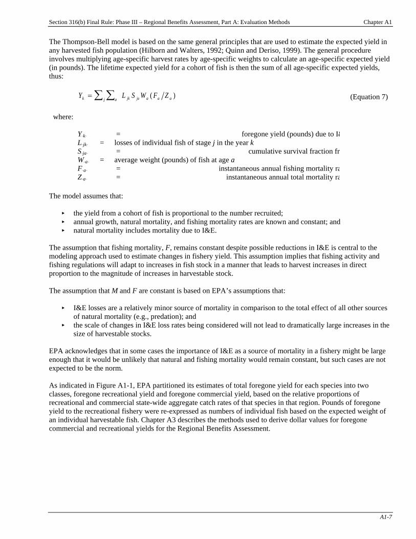
The Thompson-Bell model is based on the same general principles that are used to estimate the expected yield in any harvested fish population (Hilborn and Walters, 1992; Quinn and Deriso, 1999). The general procedure involves multiplying age-specific harvest rates by age-specific weights to calculate an age-specific expected yield (in pounds). The lifetime expected yield for a cohort of fish is then the sum of all age-specific expected yields, thus:
Y L S W Fk aj jk ja a a a= ∑∑ ( )Z
where: YBBBkBBB = foregone yield (pounds) due to I& LBBBjkBBB = losses of individual fish of stage j in the year k SBBBjaBBB = cumulative survival fraction fr WBBBaBBB = average weight (pounds) of fish at age a FBBBaBBB = instantaneous annual fishing mortality ra ZBBBaBBB = instantaneous annual total mortality ra
(Equation 7)
The model assumes that:
< the yield from a cohort of fish is proportional to the number recruited; < annual growth, natural mortality, and fishing mortality rates are known and constant; and < natural mortality includes mortality due to I&E.
The assumption that fishing mortality, F, remains constant despite possible reductions in I&E is central to the modeling approach used to estimate changes in fishery yield. This assumption implies that fishing activity and fishing regulations will adapt to increases in fish stock in a manner that leads to harvest increases in direct proportion to the magnitude of increases in harvestable stock. The assumption that M and F are constant is based on EPA’s assumptions that:
< I&E losses are a relatively minor source of mortality in comparison to the total effect of all other sources of natural mortality (e.g., predation); and
< the scale of changes in I&E loss rates being considered will not lead to dramatically large increases in the size of harvestable stocks.
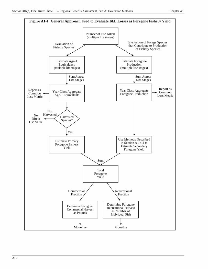
EPA acknowledges that in some cases the importance of I&E as a source of mortality in a fishery might be large enough that it would be unlikely that natural and fishing mortality would remain constant, but such cases are not expected to be the norm. As indicated in Figure A1-1, EPA partitioned its estimates of total foregone yield for each species into two classes, foregone recreational yield and foregone commercial yield, based on the relative proportions of recreational and commercial state-wide aggregate catch rates of that species in that region. Pounds of foregone yield to the recreational fishery were re-expressed as numbers of individual fish based on the expected weight of an individual harvestable fish. Chapter A3 describes the methods used to derive dollar values for foregone commercial and recreational yields for the Regional Benefits Assessment.
Section 316(b) Final Rule: Phase III – Regional Benefits Assessment, Part A: Evaluation Methods Chapter A1
A1-8
Figure A1-1: General Approach Used to Evaluate I&E Losses as Foregone Fishery Yield
TotalForegone
Yield
NotHarvestedNo
DirectUse Value
Sum AcrossLife Stages
Yes
Sum AcrossLife Stages
CommercialFraction
RecreationalFraction
Monetize Monetize
Report asCommon
Loss Metric
Sum
Report asCommon
Loss Metric
Estimate ForegoneProduction
(multiple life stages)
Year Class AggregateForegone Production
Estimate Age-1Equivalency
(multiple life stages)
Year Class AggregateAge-1 Equivalents
HarvestedSpecies?
Number of Fish Killed(multiple life stages)
Determine ForegoneRecreational Harvest
as Number ofIndividual Fish
Determine ForegoneCommercial Harvest
as Pounds
Estimate PrimaryForegone Fishery
Yield
Use Methods Describedin Section A1-4.4 toEstimate Secondary
Foregone Yield
Evaluation ofFishery Species
Evaluation of Forage Speciesthat Contribute to Production
of Fishery Species
Section 316(b) Final Rule: Phase III – Regional Benefits Assessment, Part A: Evaluation Methods Chapter A1
A1-9
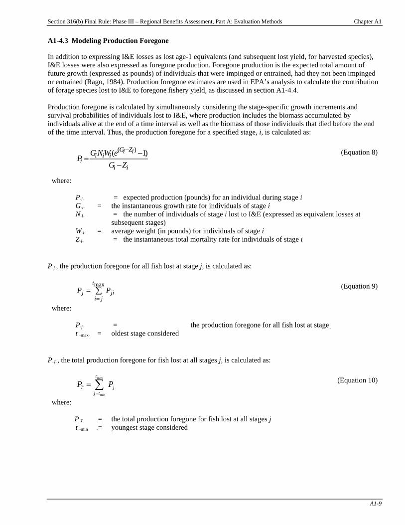
A1-4.3 Modeling Production Foregone In addition to expressing I&E losses as lost age-1 equivalents (and subsequent lost yield, for harvested species), I&E losses were also expressed as foregone production. Foregone production is the expected total amount of future growth (expressed as pounds) of individuals that were impinged or entrained, had they not been impinged or entrained (Rago, 1984). Production foregone estimates are used in EPA’s analysis to calculate the contribution of forage species lost to I&E to foregone fishery yield, as discussed in section A1-4.4. Production foregone is calculated by simultaneously considering the stage-specific growth increments and survival probabilities of individuals lost to I&E, where production includes the biomass accumulated by individuals alive at the end of a time interval as well as the biomass of those individuals that died before the end of the time interval. Thus, the production foregone for a specified stage, i, is calculated as:
ii
iZiGiii
i ZGeWNG
P−
−=
− )1( )(
(Equation 8)
where: PBBBiBBB = expected production (pounds) for an individual during stage i GBBBiBBB = the instantaneous growth rate for individuals of stage i NBBBiBBB = the number of individuals of stage i lost to I&E (expressed as equivalent losses at
subsequent stages) WBBBiBBB = average weight (in pounds) for individuals of stage i ZBBBiBBB = the instantaneous total mortality rate for individuals of stage i
PBBBjBBB, the production foregone for all fish lost at stage j, is calculated as:
jit
jij PP ∑
==
max
where: PBBBjBBB = the production foregone for all fish lost at stage j t BBBmaxBBB = oldest stage considered
(Equation 9)
PBBBTBBB, the total production foregone for fish lost at all stages j, is calculated as:
j
t
tjT PP ∑
=
=max
min where: PBBBT BBB= the total production foregone for fish lost at all stages j t BBBmin BBB= youngest stage considered
(Equation 10)
Section 316(b) Final Rule: Phase III – Regional Benefits Assessment, Part A: Evaluation Methods Chapter A1
A1-10
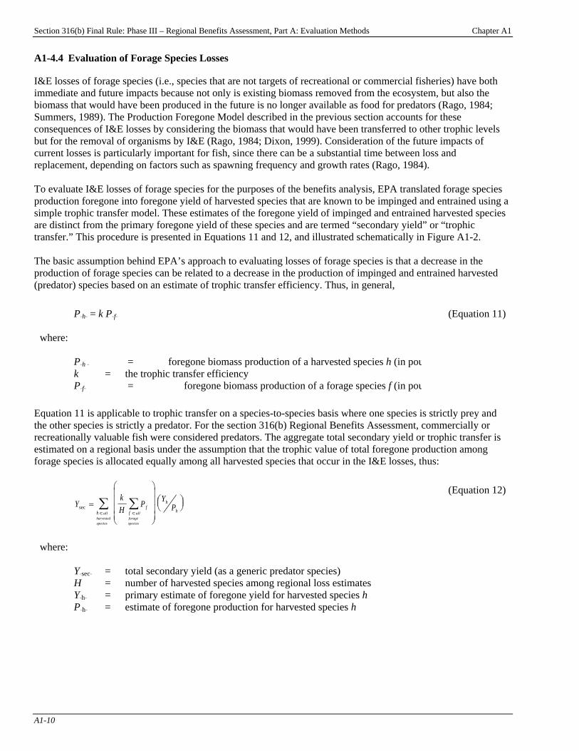
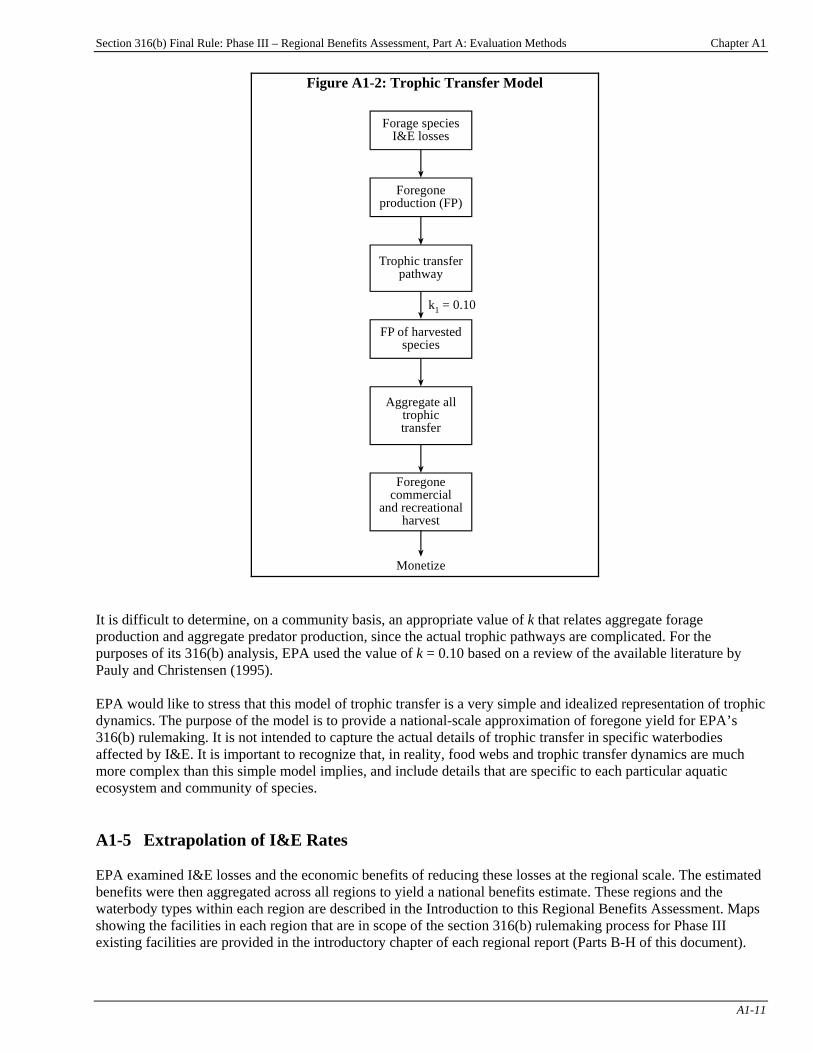
A1-4.4 Evaluation of Forage Species Losses I&E losses of forage species (i.e., species that are not targets of recreational or commercial fisheries) have both immediate and future impacts because not only is existing biomass removed from the ecosystem, but also the biomass that would have been produced in the future is no longer available as food for predators (Rago, 1984; Summers, 1989). The Production Foregone Model described in the previous section accounts for these consequences of I&E losses by considering the biomass that would have been transferred to other trophic levels but for the removal of organisms by I&E (Rago, 1984; Dixon, 1999). Consideration of the future impacts of current losses is particularly important for fish, since there can be a substantial time between loss and replacement, depending on factors such as spawning frequency and growth rates (Rago, 1984). To evaluate I&E losses of forage species for the purposes of the benefits analysis, EPA translated forage species production foregone into foregone yield of harvested species that are known to be impinged and entrained using a simple trophic transfer model. These estimates of the foregone yield of impinged and entrained harvested species are distinct from the primary foregone yield of these species and are termed “secondary yield” or “trophic transfer.” This procedure is presented in Equations 11 and 12, and illustrated schematically in Figure A1-2. The basic assumption behind EPA’s approach to evaluating losses of forage species is that a decrease in the production of forage species can be related to a decrease in the production of impinged and entrained harvested (predator) species based on an estimate of trophic transfer efficiency. Thus, in general,
PBBBhBBB = k PBBBfBBB
where: PBBBh BBB = foregone biomass production of a harvested species h (in pou k = the trophic transfer efficiency PBBBfBBB = foregone biomass production of a forage species f (in pou
(Equation 11)
Equation 11 is applicable to trophic transfer on a species-to-species basis where one species is strictly prey and the other species is strictly a predator. For the section 316(b) Regional Benefits Assessment, commercially or recreationally valuable fish were considered predators. The aggregate total secondary yield or trophic transfer is estimated on a regional basis under the assumption that the trophic value of total foregone production among forage species is allocated equally among all harvested species that occur in the I&E losses, thus:
YkH
P YP
hf
f
h
hallharvestedspecies
allforagespecies
sec =
⎛
⎝
⎜⎜⎜⎜
⎞
⎠
⎟⎟⎟⎟
⎛⎝⎜
⎞⎠⎟
∈ ∈∑ ∑
where: YBBBsecBBB = total secondary yield (as a generic predator species) H = number of harvested species among regional loss estimates YBBBhBBB = primary estimate of foregone yield for harvested species h PBBBhBBB = estimate of foregone production for harvested species h
(Equation 12)
Section 316(b) Final Rule: Phase III – Regional Benefits Assessment, Part A: Evaluation Methods Chapter A1
A1-11
Figure A1-2: Trophic Transfer Model
Monetize
FP of harvestedspecies
Foregonecommercial
and recreationalharvest
Forage speciesI&E losses
Foregoneproduction (FP)
k1 = 0.10
Trophic transferpathway
Aggregate alltrophictransfer
It is difficult to determine, on a community basis, an appropriate value of k that relates aggregate forage production and aggregate predator production, since the actual trophic pathways are complicated. For the purposes of its 316(b) analysis, EPA used the value of k = 0.10 based on a review of the available literature by Pauly and Christensen (1995). EPA would like to stress that this model of trophic transfer is a very simple and idealized representation of trophic dynamics. The purpose of the model is to provide a national-scale approximation of foregone yield for EPA’s 316(b) rulemaking. It is not intended to capture the actual details of trophic transfer in specific waterbodies affected by I&E. It is important to recognize that, in reality, food webs and trophic transfer dynamics are much more complex than this simple model implies, and include details that are specific to each particular aquatic ecosystem and community of species. A1-5 Extrapolation of I&E Rates EPA examined I&E losses and the economic benefits of reducing these losses at the regional scale. The estimated benefits were then aggregated across all regions to yield a national benefits estimate. These regions and the waterbody types within each region are described in the Introduction to this Regional Benefits Assessment. Maps showing the facilities in each region that are in scope of the section 316(b) rulemaking process for Phase III existing facilities are provided in the introductory chapter of each regional report (Parts B-H of this document).

Section 316(b) Final Rule: Phase III – Regional Benefits Assessment, Part A: Evaluation Methods Chapter A1
A1-12
To obtain regional I&E estimates, EPA extrapolated losses observed at the facilities evaluated (facilities with suitable records of I&E rates) to other in-scope facilities within the same region. Extrapolation of I&E rates from these “model” facilities was necessary because not all in scope facilities within a given region have conducted I&E studies. Model facilities included both Phase II and Phase III facilities, based on the assumption that I&E rates at Phase II and Phase III facilities are similar after normalization by intake flow. Phase II facilities were included to make use of the largest possible data set and to accommodate the lack of Phase III facility I&E studies in some regions (see Table A1-1).
Table A1-1: Number of Model Facilities, by Region and Phase of Rulemaking
Phase Region II III
California 18 0 North Atlantic 4 2 Mid-Atlantic 10 2 Gulf of Mexico 4 0 Great Lakes 8 3 Inland 30 13 South Atlantic 2 0
I&E data were extrapolated on the basis of operational flow, in millions of gallons per day (MGD), where MGD is the average operational flow over the period 1996-1998 as reported by facilities in response to EPA’s Section 316(b) Detailed Questionnaire and Short Technical Questionnaire. Operational flow at each facility was rescaled using factors reflecting the relative effectiveness of currently in-place technologies for reducing I&E. Thus, to reflect entrainment technology in place at a facility:
FBBBf,eBBB = GBBBfBBB (1-TBBBf,eBBB ) where: FBBBf,eBBB = effective relative flow rate for entrainment at facility f GBBBfBBB = mean operational flow at facility f (10PPP
6PPP gallons/day)
TBBBf,eBBB = fractional effectiveness of entrainment-reducing technology at facility f (0<TBBBf,eBBB<1)
(Equation 13)
To reflect impingement technology in place at a facility:
FBBBf,iBBB = GBBBfBBB (1-TBBBf,iBBB ) where: FBBBf,iBBB = effective relative flow rate for impingement at facility f GBBBfBBB = mean operational flow at facility f (10PPP
6PPP gallons/day)
TBBBf,iBBB = fractional effectiveness of impingement-reducing technology at facility f (0<TBBBf,iBBB<1)
(Equation 14)

Section 316(b) Final Rule: Phase III – Regional Benefits Assessment, Part A: Evaluation Methods Chapter A1
A1-13
Next, regional estimates were developed as outlined in Equations 15-18. Statistical weighting factors (from EPA’s survey of the industry) were multiplied by flow rates at each facility prior to estimating the total regional flow rate. To scale estimates for entrainment losses:
S J FAll facilitiesin region r
All model facilitiesin region r
r e f f e
f
f e
f
, ,=
∈ ∈
∑ ∑ F ,
where: SBBBr,eBBB = scaling factor to relate total entrainment losses among model
facilities to regional total entrainment losses JBBBfBBB = statistical weighting factor for facility f FBBBf,eBBB = effective relative flow rate for entrainment at facility f
(Equation 15)
To scale estimates for impingement losses:
S J FAll facilities
in region rAll model facilities
in region r
r i f f i
f
f i
f
, ,=
∈ ∈
∑ ∑ F ,
i
where: SBBBr,iBBB = scaling factor to relate total impingement losses among model facilities to regional total impingement losses JBBBfBBB = statistical weighting factor for facility f FBBBf,iBBB = effective relative flow rate for impingement at facility f
(Equation 16)
To estimate total entrainment losses for a region:
L S LAll model facilities
in region r
r e r e f ef
, , ,=∈∑
where: LBBBr,eBBB = estimated annual total entrainment losses at region r SBBBr,eBBB = scaling factor to relate total entrainment losses among model
facilities to regional total entrainment losses LBBBf,eBBB = estimated annual total entrainment losses at facility f
(Equation 17)
To estimate total impingement losses for a region:
L S Lf All model facilities in region r
r r i f, , ,i =∈
∑
where: LBBBr,i BBB= estimated annual total impingement losses at region r SBBBr,iBBB = scaling factor to relate total impingement losses among model
facilities to regional total impingement losses LBBBf,iBBB = estimated annual total impingement losses at facility f
(Equation 18)

Section 316(b) Final Rule: Phase III – Regional Benefits Assessment, Part A: Evaluation Methods Chapter A1
A1-14
EPA recognizes that there may be substantial among-facility variation in the actual I&E losses per MGD resulting from a variety of facility-specific features, such as location and type of intake structure, as well as from ecological features that affect the abundance or species composition of fish in the vicinity of each facility. The accuracy of EPA’s extrapolation procedure relies heavily on the assumption that I&E rates recorded at model facilities are representative of I&E rates at other facilities in the region. Although this assumption may not be met in some cases, limiting the extrapolation procedure to particular regions reduces the likelihood that the model facilities are unrepresentative. EPA believes that this method of extrapolation makes best use of a limited amount of empirical data, and is the only currently feasible approach for developing an estimate of national I&E and the benefits of reducing I&E. While acknowledging that an extrapolation necessarily introduces additional uncertainty into I&E estimates, EPA has not identified information that suggests that application of the procedure causes a systematic bias in the regional loss estimates. The assumption that I&E is proportional to flow is consistent with other predictive I&E studies. For example, a key assumption of the Spawning and Nursery Area of Consequence (SNAC) model (Polgar et al., 1979) is that entrainment is proportional to cooling water withdrawal rates. The SNAC model has been used as a screening tool for assessing potential I&E impacts at Chesapeake Bay plants. As a first approximation, percent entrainment has been predicted on the basis of the ratio of cooling water flow to source water flow (e.g., Goodyear, 1978). A study of power plants on the Great Lakes (Kelso and Milburn, 1979) demonstrated an increasing relationship (on a log-log scale) between plant “size” (electric production in MWe) and I&E. There is scatter in these relationships, not just because there is variation in the cooling water intake for different plants having similar electric production, but also because of the imprecision (sampling variability) inherent in the usual methods of estimating I&E. These relationships are nonetheless strong.
Section 316(b) Final Rule: Phase III – Regional Benefits Assessment, Part A: Evaluation Methods Chapter A2
A2-1
Chapter A2: Uncertainty Introduction
Chapter Contents A2-1 Types of Uncertainty.....................................A2-1 A2-1.1 Structural Uncertainty .....................A2-1 A2-1.2 Parameter Uncertainty.....................A2-2 A2-1.3 Uncertainties Related to Engineering .....................................A2-4 A2-2 Monte Carlo Analysis as a Tool for Quantifying Uncertainty ...............................A2-4 A2-3 EPA’s Uncertainty Analysis of Yield Estimates.......................................................A2-4 A2-3.1 Overview of Analysis......................A2-4 A2-3.2 Results .............................................A2-5 A2-4 Conclusions...................................................A2-6
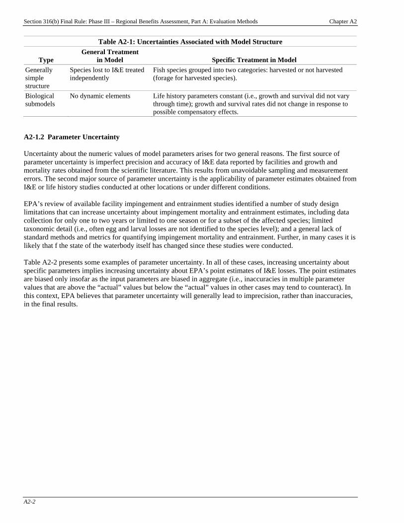
This chapter discusses sources of uncertainty in EPA’s impingement and entrainment (I&E) analyses, and presents the results of an uncertainty analysis of the yield model used by EPA to estimate the benefits of reducing I&E of commercial and recreational fishery species. Section A2-1 discusses major uncertainties in EPA’s I&E assessments, section A2-2 briefly describes Monte Carlo analysis as a tool for quantifying uncertainty, section A2-3 provides preliminary results of an uncertainty analysis by EPA of winter flounder yield estimates, and section A2-4 discusses results of the uncertainty analysis. A2-1 Types of Uncertainty Despite following sound scientific practice throughout, it was impossible to avoid several sources of uncertainty that may cause EPA’s I&E estimates in the regional analysis to be imprecise or to carry potential statistical bias. Uncertainty of this nature is not unique to EPA’s I&E analysis. Uncertainty may be classified into two general types (Finkel, 1990). One type, referred to as structural uncertainty, reflects the limits of the conceptual formulation of a model and relationships among model parameters. The other general type is parameter uncertainty, which flows from uncertainty about any of the specific numeric values of model parameters. The following discussion considers these two types of uncertainty in relation to EPA’s I&E analysis. A2-1.1 Structural Uncertainty The models used by EPA to evaluate I&E simplify a very complex process. The degree of simplification is substantial but necessary because of the limited availability of empirical data. Table A2-1 provides examples of some considerations that are not captured by the models used.
Section 316(b) Final Rule: Phase III – Regional Benefits Assessment, Part A: Evaluation Methods Chapter A2
A2-2
Table A2-1: Uncertainties Associated with Model Structure
Type General Treatment
in Model Specific Treatment in Model Generally simple structure
Species lost to I&E treated independently
Fish species grouped into two categories: harvested or not harvested (forage for harvested species).
Biological submodels
No dynamic elements Life history parameters constant (i.e., growth and survival did not vary through time); growth and survival rates did not change in response to possible compensatory effects.
A2-1.2 Parameter Uncertainty Uncertainty about the numeric values of model parameters arises for two general reasons. The first source of parameter uncertainty is imperfect precision and accuracy of I&E data reported by facilities and growth and mortality rates obtained from the scientific literature. This results from unavoidable sampling and measurement errors. The second major source of parameter uncertainty is the applicability of parameter estimates obtained from I&E or life history studies conducted at other locations or under different conditions. EPA’s review of available facility impingement and entrainment studies identified a number of study design limitations that can increase uncertainty about impingement mortality and entrainment estimates, including data collection for only one to two years or limited to one season or for a subset of the affected species; limited taxonomic detail (i.e., often egg and larval losses are not identified to the species level); and a general lack of standard methods and metrics for quantifying impingement mortality and entrainment. Further, in many cases it is likely that f the state of the waterbody itself has changed since these studies were conducted. Table A2-2 presents some examples of parameter uncertainty. In all of these cases, increasing uncertainty about specific parameters implies increasing uncertainty about EPA’s point estimates of I&E losses. The point estimates are biased only insofar as the input parameters are biased in aggregate (i.e., inaccuracies in multiple parameter values that are above the “actual” values but below the “actual” values in other cases may tend to counteract). In this context, EPA believes that parameter uncertainty will generally lead to imprecision, rather than inaccuracies, in the final results.
Section 316(b) Final Rule: Phase III – Regional Benefits Assessment, Part A: Evaluation Methods Chapter A2
A2-3
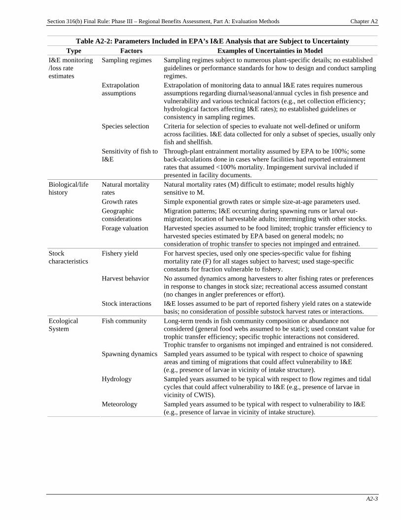
Table A2-2: Parameters Included in EPA’s I&E Analysis that are Subject to Uncertainty Type Factors Examples of Uncertainties in Model
Sampling regimes Sampling regimes subject to numerous plant-specific details; no established guidelines or performance standards for how to design and conduct sampling regimes.
Extrapolation assumptions
Extrapolation of monitoring data to annual I&E rates requires numerous assumptions regarding diurnal/seasonal/annual cycles in fish presence and vulnerability and various technical factors (e.g., net collection efficiency; hydrological factors affecting I&E rates); no established guidelines or consistency in sampling regimes.
Species selection Criteria for selection of species to evaluate not well-defined or uniform across facilities. I&E data collected for only a subset of species, usually only fish and shellfish.
I&E monitoring /loss rate estimates
Sensitivity of fish to I&E
Through-plant entrainment mortality assumed by EPA to be 100%; some back-calculations done in cases where facilities had reported entrainment rates that assumed <100% mortality. Impingement survival included if presented in facility documents.
Natural mortality rates
Natural mortality rates (M) difficult to estimate; model results highly sensitive to M.
Growth rates Simple exponential growth rates or simple size-at-age parameters used. Geographic considerations
Migration patterns; I&E occurring during spawning runs or larval out-migration; location of harvestable adults; intermingling with other stocks.
Biological/life history
Forage valuation Harvested species assumed to be food limited; trophic transfer efficiency to harvested species estimated by EPA based on general models; no consideration of trophic transfer to species not impinged and entrained.
Fishery yield For harvest species, used only one species-specific value for fishing mortality rate (F) for all stages subject to harvest; used stage-specific constants for fraction vulnerable to fishery.
Harvest behavior No assumed dynamics among harvesters to alter fishing rates or preferences in response to changes in stock size; recreational access assumed constant (no changes in angler preferences or effort).
Stock characteristics
Stock interactions I&E losses assumed to be part of reported fishery yield rates on a statewide basis; no consideration of possible substock harvest rates or interactions.
Fish community Long-term trends in fish community composition or abundance not considered (general food webs assumed to be static); used constant value for trophic transfer efficiency; specific trophic interactions not considered. Trophic transfer to organisms not impinged and entrained is not considered.
Spawning dynamics Sampled years assumed to be typical with respect to choice of spawning areas and timing of migrations that could affect vulnerability to I&E (e.g., presence of larvae in vicinity of intake structure).
Hydrology Sampled years assumed to be typical with respect to flow regimes and tidal cycles that could affect vulnerability to I&E (e.g., presence of larvae in vicinity of CWIS).
Ecological System
Meteorology Sampled years assumed to be typical with respect to vulnerability to I&E (e.g., presence of larvae in vicinity of intake structure).
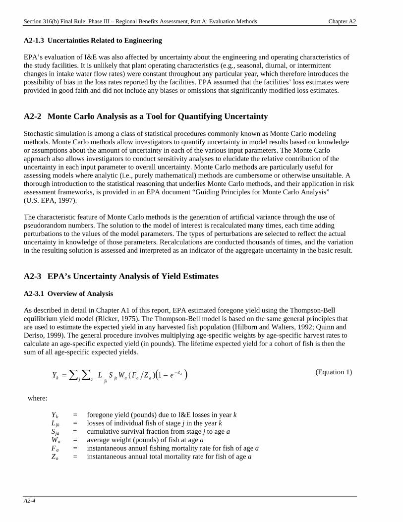
Section 316(b) Final Rule: Phase III – Regional Benefits Assessment, Part A: Evaluation Methods Chapter A2
A2-4
A2-1.3 Uncertainties Related to Engineering EPA’s evaluation of I&E was also affected by uncertainty about the engineering and operating characteristics of the study facilities. It is unlikely that plant operating characteristics (e.g., seasonal, diurnal, or intermittent changes in intake water flow rates) were constant throughout any particular year, which therefore introduces the possibility of bias in the loss rates reported by the facilities. EPA assumed that the facilities’ loss estimates were provided in good faith and did not include any biases or omissions that significantly modified loss estimates. A2-2 Monte Carlo Analysis as a Tool for Quantifying Uncertainty Stochastic simulation is among a class of statistical procedures commonly known as Monte Carlo modeling methods. Monte Carlo methods allow investigators to quantify uncertainty in model results based on knowledge or assumptions about the amount of uncertainty in each of the various input parameters. The Monte Carlo approach also allows investigators to conduct sensitivity analyses to elucidate the relative contribution of the uncertainty in each input parameter to overall uncertainty. Monte Carlo methods are particularly useful for assessing models where analytic (i.e., purely mathematical) methods are cumbersome or otherwise unsuitable. A thorough introduction to the statistical reasoning that underlies Monte Carlo methods, and their application in risk assessment frameworks, is provided in an EPA document “Guiding Principles for Monte Carlo Analysis” (U.S. EPA, 1997). The characteristic feature of Monte Carlo methods is the generation of artificial variance through the use of pseudorandom numbers. The solution to the model of interest is recalculated many times, each time adding perturbations to the values of the model parameters. The types of perturbations are selected to reflect the actual uncertainty in knowledge of those parameters. Recalculations are conducted thousands of times, and the variation in the resulting solution is assessed and interpreted as an indicator of the aggregate uncertainty in the basic result. A2-3 EPA’s Uncertainty Analysis of Yield Estimates A2-3.1 Overview of Analysis As described in detail in Chapter A1 of this report, EPA estimated foregone yield using the Thompson-Bell equilibrium yield model (Ricker, 1975). The Thompson-Bell model is based on the same general principles that are used to estimate the expected yield in any harvested fish population (Hilborn and Walters, 1992; Quinn and Deriso, 1999). The general procedure involves multiplying age-specific weights by age-specific harvest rates to calculate an age-specific expected yield (in pounds). The lifetime expected yield for a cohort of fish is then the sum of all age-specific expected yields.
( )Y L S W F Zk aj jk ja a a aZ a= −∑∑ −( ) 1 e
where: YBkB = foregone yield (pounds) due to I&E losses in year k LBjkB = losses of individual fish of stage j in the year k SBja B= cumulative survival fraction from stage j to age a WBaB = average weight (pounds) of fish at age a FBaB = instantaneous annual fishing mortality rate for fish of age a ZBaB = instantaneous annual total mortality rate for fish of age a
(Equation 1)

Section 316(b) Final Rule: Phase III – Regional Benefits Assessment, Part A: Evaluation Methods Chapter A2
A2-5
Quantifying the variance in yield estimates resulting from uncertainty in the numeric values of L, S, W, F, and Z assists in the interpretation of results, gives a sense of the precision in yield estimates, provides insight into the sensitivity of predictions to particular parameter values, and indicates the contribution of particular parameters to overall uncertainty. EPA evaluated uncertainty in yield estimates for winter flounder using I&E data for a facility located on a North Atlantic estuary. The I&E loss records and winter flounder life history parameters that were used are provided in the Phase II docket as DCN #4-2037. EPA developed a custom program written in the S language to conduct the Monte Carlo analysis. Wherever possible, the simulation tool re-used the same code that was used to calculate yield for the original assessment. Graphical displays were used to confirm the behavior of random number generation and to examine results. Selection of input distributions for parameters of interest are a key element of any Monte Carlo analysis. In the winter flounder test case, the parameter values were drawn from uniform distributions with a range defined as the initial, best estimate of the parameter +/- 15%. EPA investigated sensitivity of the model to variations in parameters by grouping the parameters into five classes:
< natural mortality (M) at all life stages; < fishing mortality (F) at all life stages; < fraction vulnerable to fishing (V) at all life stages (i.e., age of recruitment to the fishery); < weight at age (W); and < the reported I&E loss rates (L).
The analysis consisted of repeating runs (n = 10,000 in each run) of the model wherein each of the groups of parameters was either held constant at their best estimates or were varied stochastically according to the defined input distributions. The relative importance of these groups of parameters was assessed by comparing the relative amount of variation between each set of runs. Model sensitivity to individual parameters has not been examined. A2-3.2 Results For entrainment losses for this species, the analysis indicated that the yield model is most sensitive to uncertainty in natural mortality rates, followed by uncertainty in the I&E loss rates themselves (Figure A2-1). Age-specific weights were the third most important group, followed by fishing mortality and age at recruitment, which were relatively insignificant sources of uncertainty.
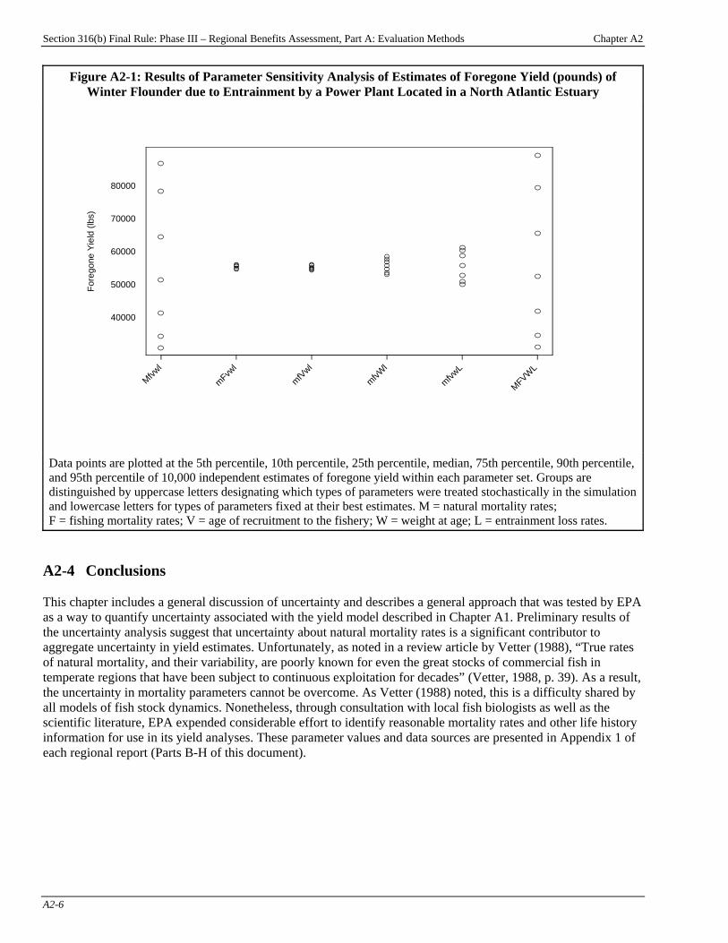
Section 316(b) Final Rule: Phase III – Regional Benefits Assessment, Part A: Evaluation Methods Chapter A2
A2-6
Figure A2-1: Results of Parameter Sensitivity Analysis of Estimates of Foregone Yield (pounds) of Winter Flounder due to Entrainment by a Power Plant Located in a North Atlantic Estuary
Mfvwl
mFvwl
mfVwl
mfvWl
mfvwL
MFVWL
40000
50000
60000
70000
80000
Fore
gone
Yie
ld (l
bs)
Data points are plotted at the 5th percentile, 10th percentile, 25th percentile, median, 75th percentile, 90th percentile, and 95th percentile of 10,000 independent estimates of foregone yield within each parameter set. Groups are distinguished by uppercase letters designating which types of parameters were treated stochastically in the simulation and lowercase letters for types of parameters fixed at their best estimates. M = natural mortality rates; F = fishing mortality rates; V = age of recruitment to the fishery; W = weight at age; L = entrainment loss rates.
A2-4 Conclusions This chapter includes a general discussion of uncertainty and describes a general approach that was tested by EPA as a way to quantify uncertainty associated with the yield model described in Chapter A1. Preliminary results of the uncertainty analysis suggest that uncertainty about natural mortality rates is a significant contributor to aggregate uncertainty in yield estimates. Unfortunately, as noted in a review article by Vetter (1988), “True rates of natural mortality, and their variability, are poorly known for even the great stocks of commercial fish in temperate regions that have been subject to continuous exploitation for decades” (Vetter, 1988, p. 39). As a result, the uncertainty in mortality parameters cannot be overcome. As Vetter (1988) noted, this is a difficulty shared by all models of fish stock dynamics. Nonetheless, through consultation with local fish biologists as well as the scientific literature, EPA expended considerable effort to identify reasonable mortality rates and other life history information for use in its yield analyses. These parameter values and data sources are presented in Appendix 1 of each regional report (Parts B-H of this document).
Section 316(b) Final Rule: Phase III – Regional Benefits Assessment, Part A: Evaluation Methods Chapter A3
A3-1
Chapter A3: Economic Benefit Categories and Valuation
Introduction Changes in cooling water intake structure (CWIS) design or operations resulting from the regulatory analysis options for the final section 316(b) rule for Phase III facilities were expected to reduce impingement and entrainment (I&E) losses of fish, shellfish, and other aquatic organisms. As a result, the regulatory analysis options were expected to increase the numbers of individuals present and increase local and regional fishery populations. The aquatic resources affected by cooling water intake structures provide a wide range of ecosystem services. Ecosystem services are the physical, chemical, and biological functions performed by natural resources and the human benefits derived from those functions, including both ecological and human use services (Daily, 1997; Daily et al., 1997). Scientific and public interest in protecting ecosystem services is increasing with the recognition that these services are vulnerable to a wide range of human activities and are difficult, if not impossible, to replace with human technologies (Meffe, 1992).
Chapter Contents A3-1 Economic Benefit Categories Applicable
to the Regulatory Analysis Options for Phase III Facilities ....................................A3-2
A3-2 Direct Use Benefits...................................A3-5 A3-3 Indirect Use Benefits ................................A3-7 A3-4 Non-Use Benefits .....................................A3-7 A3-4.1 Role of Non-Use Benefits in
the Benefits Analysis for the Regulatory Analysis Options for Phase III Facilities ......................A3-8
A3-5 Summary of Benefit Categories ...............A3-9 A3-6 Causality: Linking the Regulatory
Analysis Options for Phase III Existing Facilities to Beneficial Outcomes...........A3-11
A3-7 Conclusions ............................................A3-12
In addition to their importance in providing food and other goods of direct use to humans, the organisms lost to I&E are critical to the continued functioning of the ecosystems of which they are a part. Fish are essential for energy transfer in aquatic food webs, regulation of food web structure, nutrient cycling, maintenance of sediment processes, redistribution of bottom substrates, the regulation of carbon fluxes from water to the atmosphere, and the maintenance of aquatic biodiversity (Peterson and Lubchenco, 1997; Postel and Carpenter, 1997; Holmlund and Hammer, 1999; Wilson and Carpenter, 1999). Examples of the impact of I&E on ecological and public services include:
< decreased numbers of ecological keystone, rare, or sensitive species; < decreased numbers of popular species that are not fished, perhaps because the fishery is closed; < decreased numbers of special status (e.g., threatened or endangered) species; < increased numbers of exotic or disruptive species that compete well in the absence of species lost to I&E; < disruption of ecological niches and ecological strategies used by aquatic species; < disruption of organic carbon and nutrient transfer through the food web; < disruption of energy transfer through the food web; < decreased local biodiversity; < disruption of predator-prey relationships; < disruption of age class structures of species; < disruption of natural succession processes; < disruption of public uses other than fishing, such as diving, boating, and nature viewing; and < disruption of public satisfaction with a healthy ecosystem.

Section 316(b) Final Rule: Phase III – Regional Benefits Assessment, Part A: Evaluation Methods Chapter A3
A3-2
Many of these services can only be maintained by the continued presence of all life stages of fish and other aquatic species in their natural habitats. The traditional approach of EPA and other natural resource agencies to quantifying the environmental benefits of regulations has focused on active use values, particularly direct use values such as recreational or commercial fishing. Nonconsumptive uses (such as the importance of fish for aquatic food webs), and passive use or non-use values (including the value of protecting a resource for its own sake), are seldom separately quantified because they are difficult to monetize with available economic methods. However, even though economists debate methods for indirect and non-use valuation, there is general agreement that these values exist and can be important (Freeman, 2003). When valuations that include both use and non-use components, such as Carson and Mitchell (1993), and Mitchell and Carson (1981, 1986, and 1989) are used, non-use values are incorporated into the analysis, although they cannot be separated from use values. This chapter first identifies the types of economic benefits that are likely to be generated by improved ecosystem functioning resulting from the regulatory analysis options for Phase III facilities. Then, the chapter presents the basic economic concepts regarding economic benefits, including benefit categories and benefit taxonomies associated with market and nonmarket goods and services that are likely to flow from reduced I&E. Other chapters in this section of the report detail the methods used to estimate values for reductions in I&E. These methods are in turn applied in the regional studies described in Parts B through H of this document. A3-1 Economic Benefit Categories Applicable to the Regulatory Analysis Options for
Phase III Facilities The term “economic benefits” for our purposes refers to the dollar value associated with all of the expected positive impacts of the regulatory analysis options for Phase III facilities. The basic approach for estimating the benefits of a policy event is to evaluate changes in social welfare realized by consumers and producers. Such measures are based on standardized and widely accepted concepts within applied welfare economics. They reflect the degree of well-being derived by economic agents (e.g., people and/or firms) given different levels of goods and services, including those associated with environmental quality. For market goods, analysts typically use money-denominated measures of consumer and producer surplus, which provide an approximation of exact welfare effects (Freeman, 2003).PF
1FP For nonmarket goods, such as aquatic habitat, values must be assessed using
nonmarket valuation methods. In such cases, valuation estimates are typically restricted to effects on individual households (or consumers), and either represent consumer surplus or analogous exact Hicksian welfare measures (e.g., compensating surplus). The choice of welfare (i.e., value) measures is often determined by the valuation context. Estimating economic benefits of reducing I&E at existing CWIS can be challenging. Many steps are needed to analyze the link between reductions in I&E and improvements in human welfare. The changes produced by the new regulations on fisheries and other aspects of relevant aquatic ecosystems must be determined, and then linked in a meaningful way to the associated environmental goods and services that ultimately produce increased benefits. Key challenges in environmental benefits assessment include uncertainties, data availability, and the fact that many of the goods and services beneficially affected by CWIS are not traded in the marketplace (i.e., monetary values can not be established based on observed market transactions for some of the important beneficial outcomes). In this case, several types of benefits need to be estimated using nonmarket valuation techniques. Where this cannot be done in a reliable manner, the benefits must be described and considered qualitatively.
P
1P Technically, consumer surplus reflects the difference between the “value” an individual places on a good or
service (as reflected by the individual’s “willingness-to-pay” (WTP) for that unit of the good or service) and the “cost” incurred by that individual to acquire it (as reflected by the “price” of a commodity or service, if it is provided in the marketplace). See Chapter A4 for a more detailed discussion of consumer and producer surplus.
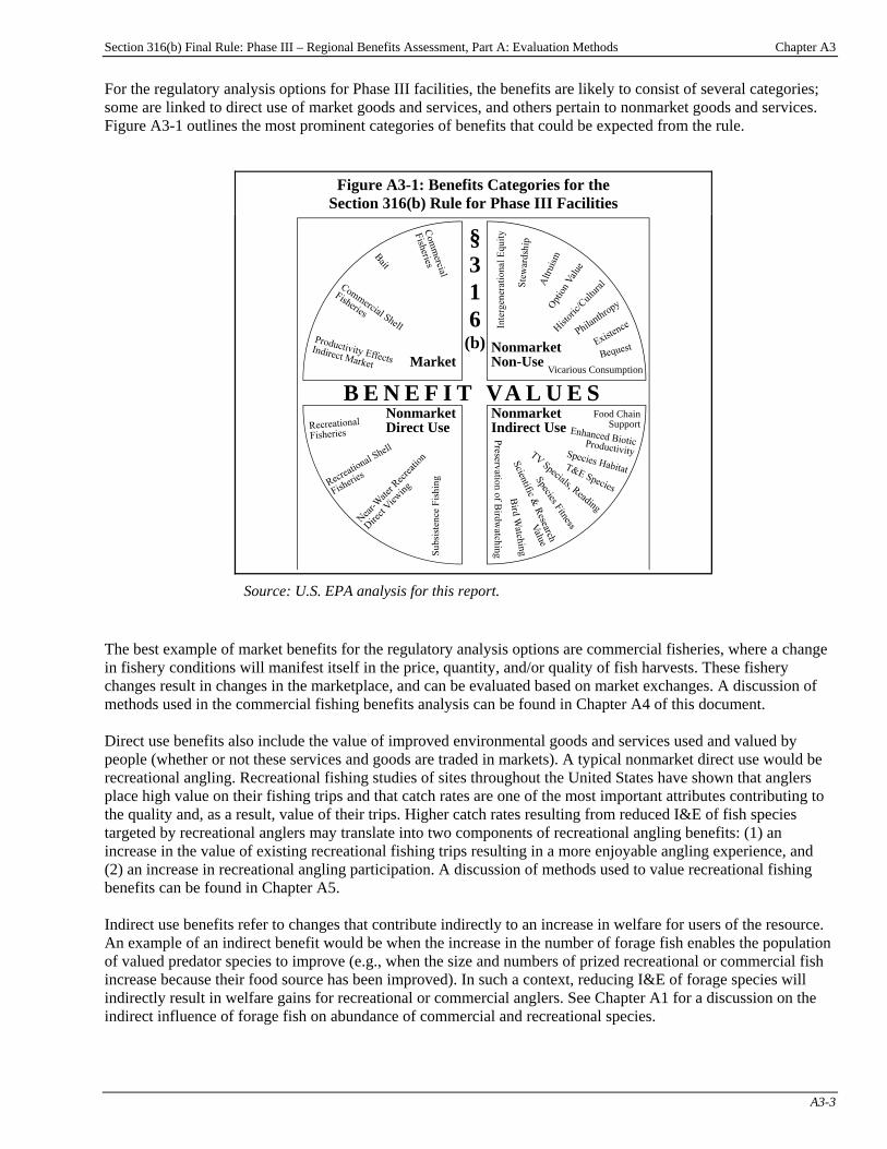
Section 316(b) Final Rule: Phase III – Regional Benefits Assessment, Part A: Evaluation Methods Chapter A3
A3-3
For the regulatory analysis options for Phase III facilities, the benefits are likely to consist of several categories; some are linked to direct use of market goods and services, and others pertain to nonmarket goods and services. Figure A3-1 outlines the most prominent categories of benefits that could be expected from the rule.
Figure A3-1: Benefits Categories for the Section 316(b) Rule for Phase III Facilities
B E N E F I T VA L U E S
§316
(b)Market
NonmarketDirect Use
NonmarketIndirect Use
NonmarketNon-Use
Vicarious Consumption
Food ChainSupport
Source: U.S. EPA analysis for this report.
The best example of market benefits for the regulatory analysis options are commercial fisheries, where a change in fishery conditions will manifest itself in the price, quantity, and/or quality of fish harvests. These fishery changes result in changes in the marketplace, and can be evaluated based on market exchanges. A discussion of methods used in the commercial fishing benefits analysis can be found in Chapter A4 of this document. Direct use benefits also include the value of improved environmental goods and services used and valued by people (whether or not these services and goods are traded in markets). A typical nonmarket direct use would be recreational angling. Recreational fishing studies of sites throughout the United States have shown that anglers place high value on their fishing trips and that catch rates are one of the most important attributes contributing to the quality and, as a result, value of their trips. Higher catch rates resulting from reduced I&E of fish species targeted by recreational anglers may translate into two components of recreational angling benefits: (1) an increase in the value of existing recreational fishing trips resulting in a more enjoyable angling experience, and (2) an increase in recreational angling participation. A discussion of methods used to value recreational fishing benefits can be found in Chapter A5. Indirect use benefits refer to changes that contribute indirectly to an increase in welfare for users of the resource. An example of an indirect benefit would be when the increase in the number of forage fish enables the population of valued predator species to improve (e.g., when the size and numbers of prized recreational or commercial fish increase because their food source has been improved). In such a context, reducing I&E of forage species will indirectly result in welfare gains for recreational or commercial anglers. See Chapter A1 for a discussion on the indirect influence of forage fish on abundance of commercial and recreational species.
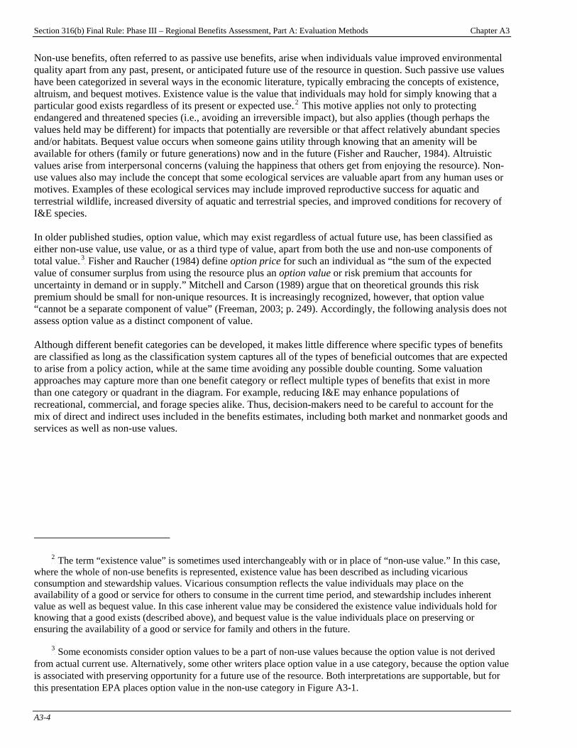
Section 316(b) Final Rule: Phase III – Regional Benefits Assessment, Part A: Evaluation Methods Chapter A3
A3-4
Non-use benefits, often referred to as passive use benefits, arise when individuals value improved environmental quality apart from any past, present, or anticipated future use of the resource in question. Such passive use values have been categorized in several ways in the economic literature, typically embracing the concepts of existence, altruism, and bequest motives. Existence value is the value that individuals may hold for simply knowing that a particular good exists regardless of its present or expected use.PF
2FP This motive applies not only to protecting
endangered and threatened species (i.e., avoiding an irreversible impact), but also applies (though perhaps the values held may be different) for impacts that potentially are reversible or that affect relatively abundant species and/or habitats. Bequest value occurs when someone gains utility through knowing that an amenity will be available for others (family or future generations) now and in the future (Fisher and Raucher, 1984). Altruistic values arise from interpersonal concerns (valuing the happiness that others get from enjoying the resource). Non-use values also may include the concept that some ecological services are valuable apart from any human uses or motives. Examples of these ecological services may include improved reproductive success for aquatic and terrestrial wildlife, increased diversity of aquatic and terrestrial species, and improved conditions for recovery of I&E species. In older published studies, option value, which may exist regardless of actual future use, has been classified as either non-use value, use value, or as a third type of value, apart from both the use and non-use components of total value.PF
3FP Fisher and Raucher (1984) define option price for such an individual as “the sum of the expected
value of consumer surplus from using the resource plus an option value or risk premium that accounts for uncertainty in demand or in supply.” Mitchell and Carson (1989) argue that on theoretical grounds this risk premium should be small for non-unique resources. It is increasingly recognized, however, that option value “cannot be a separate component of value” (Freeman, 2003; p. 249). Accordingly, the following analysis does not assess option value as a distinct component of value. Although different benefit categories can be developed, it makes little difference where specific types of benefits are classified as long as the classification system captures all of the types of beneficial outcomes that are expected to arise from a policy action, while at the same time avoiding any possible double counting. Some valuation approaches may capture more than one benefit category or reflect multiple types of benefits that exist in more than one category or quadrant in the diagram. For example, reducing I&E may enhance populations of recreational, commercial, and forage species alike. Thus, decision-makers need to be careful to account for the mix of direct and indirect uses included in the benefits estimates, including both market and nonmarket goods and services as well as non-use values.
P
2P The term “existence value” is sometimes used interchangeably with or in place of “non-use value.” In this case,
where the whole of non-use benefits is represented, existence value has been described as including vicarious consumption and stewardship values. Vicarious consumption reflects the value individuals may place on the availability of a good or service for others to consume in the current time period, and stewardship includes inherent value as well as bequest value. In this case inherent value may be considered the existence value individuals hold for knowing that a good exists (described above), and bequest value is the value individuals place on preserving or ensuring the availability of a good or service for family and others in the future.
P
3P Some economists consider option values to be a part of non-use values because the option value is not derived
from actual current use. Alternatively, some other writers place option value in a use category, because the option value is associated with preserving opportunity for a future use of the resource. Both interpretations are supportable, but for this presentation EPA places option value in the non-use category in Figure A3-1.
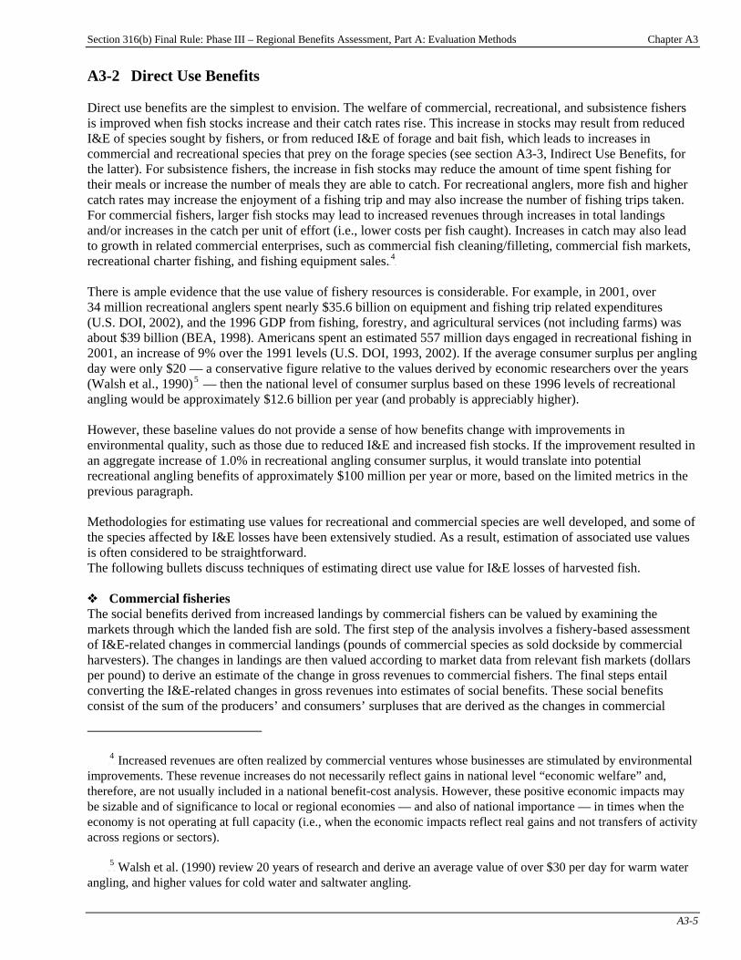
Section 316(b) Final Rule: Phase III – Regional Benefits Assessment, Part A: Evaluation Methods Chapter A3
A3-5
A3-2 Direct Use Benefits Direct use benefits are the simplest to envision. The welfare of commercial, recreational, and subsistence fishers is improved when fish stocks increase and their catch rates rise. This increase in stocks may result from reduced I&E of species sought by fishers, or from reduced I&E of forage and bait fish, which leads to increases in commercial and recreational species that prey on the forage species (see section A3-3, Indirect Use Benefits, for the latter). For subsistence fishers, the increase in fish stocks may reduce the amount of time spent fishing for their meals or increase the number of meals they are able to catch. For recreational anglers, more fish and higher catch rates may increase the enjoyment of a fishing trip and may also increase the number of fishing trips taken. For commercial fishers, larger fish stocks may lead to increased revenues through increases in total landings and/or increases in the catch per unit of effort (i.e., lower costs per fish caught). Increases in catch may also lead to growth in related commercial enterprises, such as commercial fish cleaning/filleting, commercial fish markets, recreational charter fishing, and fishing equipment sales.PF
4FP
There is ample evidence that the use value of fishery resources is considerable. For example, in 2001, over 34 million recreational anglers spent nearly $35.6 billion on equipment and fishing trip related expenditures (U.S. DOI, 2002), and the 1996 GDP from fishing, forestry, and agricultural services (not including farms) was about $39 billion (BEA, 1998). Americans spent an estimated 557 million days engaged in recreational fishing in 2001, an increase of 9% over the 1991 levels (U.S. DOI, 1993, 2002). If the average consumer surplus per angling day were only $20 — a conservative figure relative to the values derived by economic researchers over the years (Walsh et al., 1990)PF
5FP — then the national level of consumer surplus based on these 1996 levels of recreational
angling would be approximately $12.6 billion per year (and probably is appreciably higher). However, these baseline values do not provide a sense of how benefits change with improvements in environmental quality, such as those due to reduced I&E and increased fish stocks. If the improvement resulted in an aggregate increase of 1.0% in recreational angling consumer surplus, it would translate into potential recreational angling benefits of approximately $100 million per year or more, based on the limited metrics in the previous paragraph. Methodologies for estimating use values for recreational and commercial species are well developed, and some of the species affected by I&E losses have been extensively studied. As a result, estimation of associated use values is often considered to be straightforward. The following bullets discuss techniques of estimating direct use value for I&E losses of harvested fish. ˜ Commercial fisheries The social benefits derived from increased landings by commercial fishers can be valued by examining the markets through which the landed fish are sold. The first step of the analysis involves a fishery-based assessment of I&E-related changes in commercial landings (pounds of commercial species as sold dockside by commercial harvesters). The changes in landings are then valued according to market data from relevant fish markets (dollars per pound) to derive an estimate of the change in gross revenues to commercial fishers. The final steps entail converting the I&E-related changes in gross revenues into estimates of social benefits. These social benefits consist of the sum of the producers’ and consumers’ surpluses that are derived as the changes in commercial
P
4P Increased revenues are often realized by commercial ventures whose businesses are stimulated by environmental
improvements. These revenue increases do not necessarily reflect gains in national level “economic welfare” and, therefore, are not usually included in a national benefit-cost analysis. However, these positive economic impacts may be sizable and of significance to local or regional economies — and also of national importance — in times when the economy is not operating at full capacity (i.e., when the economic impacts reflect real gains and not transfers of activity across regions or sectors).
P
5P Walsh et al. (1990) review 20 years of research and derive an average value of over $30 per day for warm water
angling, and higher values for cold water and saltwater angling.
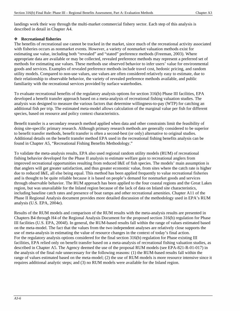
Section 316(b) Final Rule: Phase III – Regional Benefits Assessment, Part A: Evaluation Methods Chapter A3
A3-6
landings work their way through the multi-market commercial fishery sector. Each step of this analysis is described in detail in Chapter A4. ˜ Recreational fisheries The benefits of recreational use cannot be tracked in the market, since much of the recreational activity associated with fisheries occurs as nonmarket events. However, a variety of nonmarket valuation methods exist for estimating use value, including both “revealed” and “stated” preference methods (Freeman, 2003). Where appropriate data are available or may be collected, revealed preference methods may represent a preferred set of methods for estimating use values. These methods use observed behavior to infer users’ value for environmental goods and services. Examples of revealed preference methods include travel cost, hedonic pricing, and random utility models. Compared to non-use values, use values are often considered relatively easy to estimate, due to their relationship to observable behavior, the variety of revealed preference methods available, and public familiarity with the recreational services provided by surface waterbodies. To evaluate recreational benefits of the regulatory analysis options for section 316(b) Phase III facilities, EPA developed a benefit transfer approach based on a meta-analysis of recreational fishing valuation studies. The analysis was designed to measure the various factors that determine willingness-to-pay (WTP) for catching an additional fish per trip. The estimated meta-model allows calculation of the marginal value per fish for different species, based on resource and policy context characteristics. Benefit transfer is a secondary research method applied when data and other constraints limit the feasibility of doing site-specific primary research. Although primary research methods are generally considered to be superior to benefit transfer methods, benefit transfer is often a second-best (or only) alternative to original studies. Additional details on the benefit transfer method EPA used in the recreational fishing benefits analysis can be found in Chapter A5, “Recreational Fishing Benefits Methodology.” To validate the meta-analysis results, EPA also used regional random utility models (RUM) of recreational fishing behavior developed for the Phase II analysis to estimate welfare gain to recreational anglers from improved recreational opportunities resulting from reduced I&E of fish species. The models’ main assumption is that anglers will get greater satisfaction, and thus greater economic value, from sites where the catch rate is higher due to reduced I&E, all else being equal. This method has been applied frequently to value recreational fisheries and is thought to be quite reliable because it is based on people’s demand for nonmarket goods and services through observable behavior. The RUM approach has been applied to the four coastal regions and the Great Lakes region, but was unavailable for the Inland region because of the lack of data on Inland site characteristics, including baseline catch rates and presence of boat ramps and other recreational amenities. Chapter A11 of the Phase II Regional Analysis document provides more detailed discussion of the methodology used in EPA’s RUM analysis (U.S. EPA, 2004e). Results of the RUM models and comparison of the RUM results with the meta-analysis results are presented in Chapters B4 through H4 of the Regional Analysis Document for the proposed section 316(b) regulation for Phase III facilities (U.S. EPA, 2004f). In general, the RUM-based results fall within the range of values estimated based on the meta-model. The fact that the values from the two independent analyses are relatively close supports the use of meta-analysis in estimating the value of resource changes in the context of today’s final action. For the regulatory analysis options considered for the final section 316(b) regulation for Phase existing III facilities, EPA relied only on benefit transfer based on a meta-analysis of recreational fishing valuation studies, as described in Chapter A5. The Agency deemed the use of the proposal RUM models (see EPA-821-R-01-017) in the analysis of the final rule unnecessary for the following reasons: (1) the RUM-based results fall within the range of values estimated based on the meta-model; (2) the use of RUM models is more resource intensive since it requires additional analytic steps; and (3) no RUM models were available for the Inland region.

Section 316(b) Final Rule: Phase III – Regional Benefits Assessment, Part A: Evaluation Methods Chapter A3
A3-7
˜ Avoiding double-counting of direct use benefits Many of the fish species affected by I&E at CWIS sites are harvested both recreationally and commercially. To avoid double-counting the economic impacts of I&E of these species, the Agency determined the proportions of total species landings attributable to recreational and commercial fishing, and applied these proportions to the total number of affected fish. ˜ Subsistence anglers Subsistence use of fishery resources can be an important issue in areas where socioeconomic conditions (e.g., the number of low income households) or the mix of ethnic backgrounds make such angling economically or culturally important to a component of the community. In cases of Native American use of affected fisheries, the value of an improvement can sometimes be inferred from settlements in legal cases (e.g., compensation agreements between affected Tribes and various government or other institutions in cases of resource acquisitions or resource use restrictions). For more general populations, the value of improved subsistence fisheries may be estimated from the costs saved in acquiring alternative food sources (assuming the meals are replaced rather than foregone). This method may underestimate the value of a subsistence-fishery meal to the extent that the store-bought foods may be less preferred by some individuals than consuming a fresh-caught fish. Subsistence fishery benefits are not included in EPA’s regional analyses. Impacts on subsistence anglers may constitute an important environmental justice consideration, leading to underestimation of the total benefits of the regulatory analysis options. A3-3 Indirect Use Benefits Indirect use benefits refer to welfare improvements that arise for those individuals whose activities are enhanced as an indirect consequence of fishery or habitat improvements generated by the regulatory analysis options for Phase III existing facilities. For example, the options’ positive impacts on local fisheries may generate an improvement in the population levels and/or diversity of fish-eating bird species. In turn, avid bird watchers might obtain greater enjoyment from their outings, as they are more likely to see a wider mix or greater numbers of birds. The increased welfare of the bird watchers is thus an indirect consequence of the regulatory analysis options’ initial impact on fish. Another example of potential indirect benefits concerns forage species. An improvement in the population of a forage fish species may not be of any direct consequence to recreational or commercial anglers. However, the increased presence of forage fish will have an indirect affect on commercial and recreational fishing values if it increases food supplies for commercial and recreational predatory species. Thus, direct improvements in forage species populations can result in a greater number (and/or greater individual size) of those fish that are targeted by recreational or commercial anglers. In such an instance, the incremental increase in recreational and commercial fishery benefits would be an indirect consequence of the regulatory analysis options’ effect on forage fish populations. A3-4 Non-Use Benefits In contrast to direct use values, non-use values are often considered more difficult to estimate. Stated preference methods, or benefit transfer based on stated preference studies, are the generally accepted techniques for estimating these values (U.S. EPA, 2000a; U.S. OMB, 2003). Stated preference methods rely on carefully designed surveys, which either (1) ask people about their WTP for particular ecological improvements, such as increased protection of aquatic species or habitats with particular attributes, or (2) ask people to choose between competing hypothetical “packages” of ecological improvements and household cost. In either case, values are estimated by statistical analysis of survey responses.

Section 316(b) Final Rule: Phase III – Regional Benefits Assessment, Part A: Evaluation Methods Chapter A3
A3-8
Non-use values may be more difficult to assess than use values for several reasons. First, non-use values are not associated with easily observable behavior. Second, non-use values may be held by both users and non-users of a resource. Because non-users may be less familiar with particular services provided by a resource, their values may be different from the non-use values for users of the same resource. Third, the development of a defensible stated preference survey is often a time and resource intensive process. Fourth, even carefully designed surveys may be subject to certain biases associated with the hypothetical nature of survey responses (Mitchell and Carson, 1989). Finally, efforts to disaggregate total WTP into its use and non-use components have proved troublesome (Carson et al., 1999). EPA routinely estimates changes in use values of affected resources as part of regulatory development. However, given EPA’s regulatory schedule, developing and implementing stated preference surveys to elicit total value (i.e., non-use and use) of environmental quality changes resulting from environmental regulations is often not feasible. An extensive body of environmental economics literature demonstrates the importance of valuing all service losses, rather than just readily measured direct use losses. These studies typically reveal that the public holds significant value for service flows from natural resources well beyond those associated with direct uses (Fisher and Raucher, 1984; Brown, 1993; Boyd et al., 2001; Fischman, 2001; Heal et al., 2001; Herman et al., 2001; Ruhl and Gregg, 2001; Salzman et al., 2001; Wainger et al., 2001). Studies have documented public values for the non-use services provided by a variety of natural resources potentially affected by environmental impacts, including fish and wildlife (Stevens et al., 1991; Loomis et al., 2000); wetlands (Woodward and Wui, 2001); wilderness (Walsh et al., 1984); critical habitat for threatened and endangered (T&E) species (Whitehead and Blomquist, 1991; Hagen et al., 1992; Loomis and Ekstrand, 1997); overuse of groundwater (Feinerman and Knapp, 1983); hurricane impacts on wetlands (Farber, 1987); global climate change on forests (Layton and Brown, 1998); bacterial impacts on coastal ponds (Kaoru, 1993); oil impacts on surface water (Cohen, 1986); toxic substance impacts on wetlands (Hanemann et al., 1991); shoreline quality (Grigalunas et al., 1988); and beaches, shorebirds, and marine mammals (Rowe et al., 1992). Reducing I&E losses of fish and shellfish may result in both use and non-use benefits. Of the organisms that are anticipated to be protected by the regulatory analysis options for the section 316(b) regulation for Phase III facilities, approximately 2.6% will eventually be harvested by commercial and recreational fishers and therefore can be valued with direct use valuation techniques. Unharvested fish, which have no direct use value, represent 97.4% of the total loss. These unlanded fish include forage fish and the unlanded portion of the stock of harvested species. Because unlanded fish contribute to the yield of harvested fish, they have an indirect use value that is captured by the direct use value of the fish that are caught. However, this indirect use value represents only a portion of the total value of unlanded fish. Society may value both landed and unlanded fish for reasons unrelated to their use value. Such non-use values include the value that people may hold simply for knowing these fish exist. EPA believes it is important to consider non-use values. See memorandum entitled “Development of Willingness to Pay Survey Instrument for Section 316(b) Phase III Cooling Water Intake Structures” (Abt Associates, 2006) for more information on efforts to quantify non-use values. To assess public policy significance or importance of the ecological gains from the regulatory analysis options for Phase III facilities, EPA considered non-use benefits of the options qualitatively. Chapter A6 provides a qualitative assessment of non-use benefits stemming from the regulatory analysis options. Approaches to valuing I&E impacts on special status species are examined in Chapter A9. A3-4.1 Role of Non-Use Benefits in the Benefits Analysis for the Regulatory Analysis Options for Phase III
Facilities Accounting for non-use values in the Phase III benefits analysis is important because the portion of I&E losses consisting of organisms that may be valued through measuring direct human use value () represent only portion of the organisms impinged and entrained by CWIS. Unlanded fish include forage fish and the unlanded portion of the stock of harvested species. The value to the public of unlanded fish has two sources: (1) their indirect use as both food and breeding population for fish that are harvested; and (2) their non-use value, the value that people may hold simply for knowing these fish exist, stemming from a sense of altruism, stewardship, bequest, or
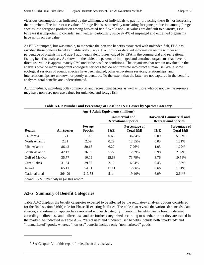
Section 316(b) Final Rule: Phase III – Regional Benefits Assessment, Part A: Evaluation Methods Chapter A3
A3-9
vicarious consumption, as indicated by the willingness of individuals to pay for protecting these fish or increasing their numbers. The indirect use value of forage fish is estimated by translating foregone production among forage species into foregone production among harvested fish.PF
6FP While non-use values are difficult to quantify, EPA
believes it is important to consider such values, particularly since 97.4% of impinged and entrained organisms have no direct use value. As EPA attempted, but was unable, to monetize the non-use benefits associated with unlanded fish, EPA has ascribed these non-use benefits qualitatively. Table A3-1 provides detailed information on the number and percentage of organisms and age-1 adult equivalent losses valued by EPA in the commercial and recreational fishing benefits analyses. As shown in the table, the percent of impinged and entrained organisms that have no direct use value is approximately 97% under the baseline conditions. The organisms that remain unvalued in the analysis provide many important ecological services that do not translate into direct human use. While some ecological services of aquatic species have been studied, other ecosystems services, relationships, and interrelationships are unknown or poorly understood. To the extent that the latter are not captured in the benefits analyses, total benefits are underestimated. All individuals, including both commercial and recreational fishers as well as those who do not use the resource, may have non-zero non-use values for unlanded and forage fish.
Table A3-1: Number and Percentage of Baseline I&E Losses by Species Category Age-1 Adult Equivalents (millions)
Commercial and Recreational Species
Harvested Commercial and Recreational Species
Region All Species
Forage Species I&E
Percentage of Total I&E I&E
Percentage of Total I&E
California 1.71 1.08 0.63 36.84% 0.09 5.38% North Atlantic 2.31 2.02 0.29 12.55% 0.03 1.21% Mid-Atlantic 86.42 80.15 6.27 7.26% 1.05 1.22% South Atlantic 42.12 36.89 5.22 12.39% 0.98 2.32% Gulf of Mexico 35.77 10.09 25.68 71.79% 3.76 10.51% Great Lakes 31.54 29.35 2.19 6.94% 0.43 1.35% Inland 65.11 54.01 11.11 17.06% 0.66 1.01% National total 264.99 213.58 51.4 19.40% 6.99 2.64% Source: U.S. EPA analysis for this report. A3-5 Summary of Benefit Categories Table A3-2 displays the benefit categories expected to be affected by the regulatory analysis options considered for the final section 316(b) rule for Phase III existing facilities. The table also reveals the various data needs, data sources, and estimation approaches associated with each category. Economic benefits can be broadly defined according to direct use and indirect use, and are further categorized according to whether or not they are traded in the market. As indicated in Table A3-2, “direct use” and “indirect use” benefits include both “marketed” and “nonmarketed” goods, whereas “non-use” benefits include only “nonmarketed” goods.
P
6P See Chapter A1 of this report for details on this analysis.
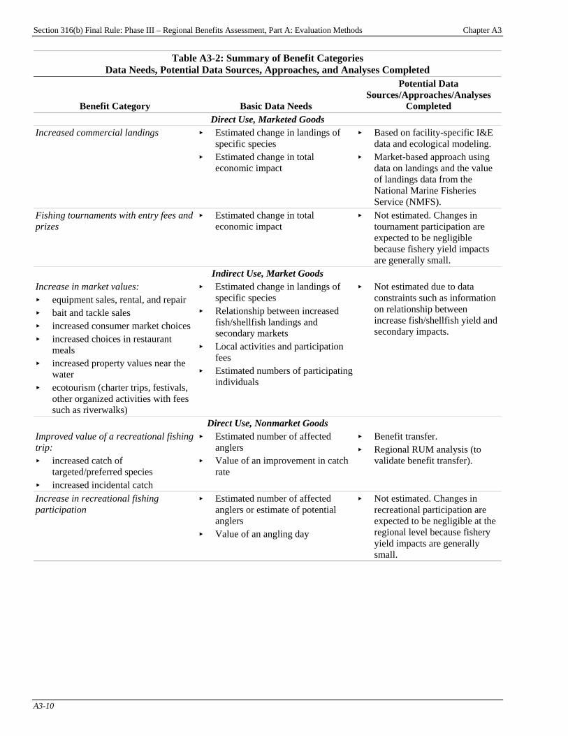
Section 316(b) Final Rule: Phase III – Regional Benefits Assessment, Part A: Evaluation Methods Chapter A3
A3-10
Table A3-2: Summary of Benefit Categories Data Needs, Potential Data Sources, Approaches, and Analyses Completed
Benefit Category Basic Data Needs
Potential Data Sources/Approaches/Analyses
Completed Direct Use, Marketed Goods
Increased commercial landings
< Estimated change in landings of specific species
< Estimated change in total economic impact
< Based on facility-specific I&E data and ecological modeling.
< Market-based approach using data on landings and the value of landings data from the National Marine Fisheries Service (NMFS).
Fishing tournaments with entry fees and prizes
< Estimated change in total economic impact
< Not estimated. Changes in tournament participation are expected to be negligible because fishery yield impacts are generally small.
Indirect Use, Market Goods Increase in market values: < equipment sales, rental, and repair < bait and tackle sales < increased consumer market choices < increased choices in restaurant
meals < increased property values near the
water < ecotourism (charter trips, festivals,
other organized activities with fees such as riverwalks)
< Estimated change in landings of specific species
< Relationship between increased fish/shellfish landings and secondary markets
< Local activities and participation fees
< Estimated numbers of participating individuals
< Not estimated due to data constraints such as information on relationship between increase fish/shellfish yield and secondary impacts.
Direct Use, Nonmarket Goods Improved value of a recreational fishing trip: < increased catch of
targeted/preferred species < increased incidental catch
< Estimated number of affected anglers
< Value of an improvement in catch rate
< Benefit transfer. < Regional RUM analysis (to
validate benefit transfer).
Increase in recreational fishing participation
< Estimated number of affected anglers or estimate of potential anglers
< Value of an angling day
< Not estimated. Changes in recreational participation are expected to be negligible at the regional level because fishery yield impacts are generally small.
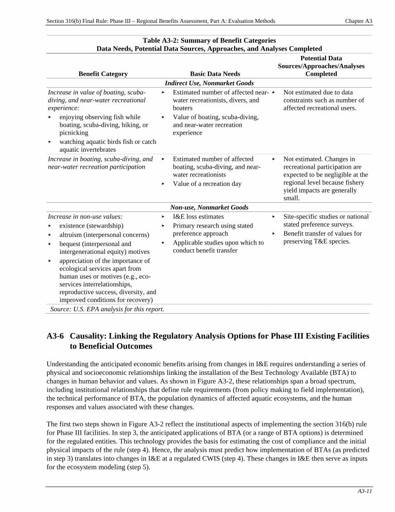
Section 316(b) Final Rule: Phase III – Regional Benefits Assessment, Part A: Evaluation Methods Chapter A3
A3-11
Table A3-2: Summary of Benefit Categories Data Needs, Potential Data Sources, Approaches, and Analyses Completed
Benefit Category Basic Data Needs
Potential Data Sources/Approaches/Analyses
Completed Indirect Use, Nonmarket Goods
Increase in value of boating, scuba-diving, and near-water recreational experience: < enjoying observing fish while
boating, scuba-diving, hiking, or picnicking
< watching aquatic birds fish or catch aquatic invertebrates
< Estimated number of affected near-water recreationists, divers, and boaters
< Value of boating, scuba-diving, and near-water recreation experience
< Not estimated due to data constraints such as number of affected recreational users.
Increase in boating, scuba-diving, and near-water recreation participation
< Estimated number of affected boating, scuba-diving, and near-water recreationists
< Value of a recreation day
< Not estimated. Changes in recreational participation are expected to be negligible at the regional level because fishery yield impacts are generally small.
Non-use, Nonmarket Goods Increase in non-use values: < existence (stewardship) < altruism (interpersonal concerns) < bequest (interpersonal and
intergenerational equity) motives < appreciation of the importance of
ecological services apart from human uses or motives (e.g., eco-services interrelationships, reproductive success, diversity, and improved conditions for recovery)
< I&E loss estimates < Primary research using stated
preference approach < Applicable studies upon which to
conduct benefit transfer
< Site-specific studies or national stated preference surveys.
< Benefit transfer of values for preserving T&E species.
Source: U.S. EPA analysis for this report. A3-6 Causality: Linking the Regulatory Analysis Options for Phase III Existing Facilities
to Beneficial Outcomes Understanding the anticipated economic benefits arising from changes in I&E requires understanding a series of physical and socioeconomic relationships linking the installation of the Best Technology Available (BTA) to changes in human behavior and values. As shown in Figure A3-2, these relationships span a broad spectrum, including institutional relationships that define rule requirements (from policy making to field implementation), the technical performance of BTA, the population dynamics of affected aquatic ecosystems, and the human responses and values associated with these changes. The first two steps shown in Figure A3-2 reflect the institutional aspects of implementing the section 316(b) rule for Phase III facilities. In step 3, the anticipated applications of BTA (or a range of BTA options) is determined for the regulated entities. This technology provides the basis for estimating the cost of compliance and the initial physical impacts of the rule (step 4). Hence, the analysis must predict how implementation of BTAs (as predicted in step 3) translates into changes in I&E at a regulated CWIS (step 4). These changes in I&E then serve as inputs for the ecosystem modeling (step 5).
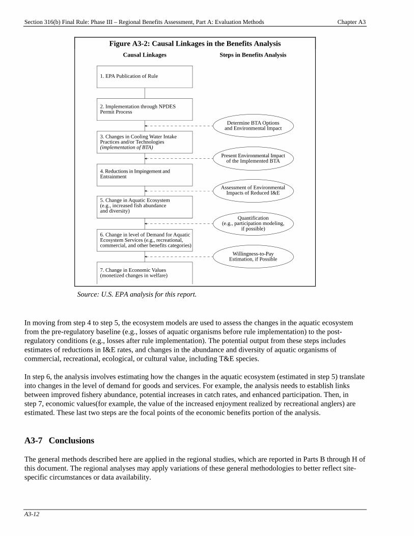
Section 316(b) Final Rule: Phase III – Regional Benefits Assessment, Part A: Evaluation Methods Chapter A3
A3-12
Figure A3-2: Causal Linkages in the Benefits Analysis Steps in Benefits Analysis
1. EPA Publication of Rule
7. Change in Economic Values(monetized changes in welfare)
2. Implementation through NPDESPermit Process
Assessment of EnvironmentalImpacts of Reduced I&E
Present Environmental Impactof the Implemented BTA
Determine BTA Optionsand Environmental Impact
6. Change in level of Demand for AquaticEcosystem Services (e.g., recreational,commercial, and other benefits categories)
5. Change in Aquatic Ecosystem(e.g., increased fish abundanceand diversity)
4. Reductions in Impingement andEntrainment
3. Changes in Cooling Water IntakePractices and/or Technologies(implementation of BTA)
Willingness-to-PayEstimation, if Possible
Quantification(e.g., participation modeling,
if possible)
Causal Linkages
Source: U.S. EPA analysis for this report. In moving from step 4 to step 5, the ecosystem models are used to assess the changes in the aquatic ecosystem from the pre-regulatory baseline (e.g., losses of aquatic organisms before rule implementation) to the post-regulatory conditions (e.g., losses after rule implementation). The potential output from these steps includes estimates of reductions in I&E rates, and changes in the abundance and diversity of aquatic organisms of commercial, recreational, ecological, or cultural value, including T&E species. In step 6, the analysis involves estimating how the changes in the aquatic ecosystem (estimated in step 5) translate into changes in the level of demand for goods and services. For example, the analysis needs to establish links between improved fishery abundance, potential increases in catch rates, and enhanced participation. Then, in step 7, economic values(for example, the value of the increased enjoyment realized by recreational anglers) are estimated. These last two steps are the focal points of the economic benefits portion of the analysis. A3-7 Conclusions The general methods described here are applied in the regional studies, which are reported in Parts B through H of this document. The regional analyses may apply variations of these general methodologies to better reflect site-specific circumstances or data availability.
Section 316(b) Final Rule: Phase III – Regional Benefits Assessment, Part A: Evaluation Methods Chapter A4
A4-1
Chapter A4: Methods for Estimating Commercial Fishing Benefits
Introduction
Chapter Contents A4-1 Overview of the Commercial Fisheries Sector.... A4-1 A4-1.1 Commercial Fishers ............................... A4-2 A4-1.2 Processors, Wholesalers, and Other
Middlemen............................................. A4-2 A4-1.3 Final Consumers .................................... A4-2 A4-2 The Role of Fishing Regulations and Regulatory
Participants .......................................................... A4-2 A4-3 Overview of U.S. Commercial Fisheries............. A4-4 A4-4 Prices, Quantities, Gross Revenue, and
Economic Surplus ............................................... A4-5 A4-4.1 Accuracy of Price and Quantity Data .... A4-5 A4-4.2 The Impact of Potential Price Effects .... A4-6 A4-4.3 Key Concepts Applicable to the Analysis of Revenues and Surplus......... A4-7 A4-4.4 Estimating Changes in Price
(as applicable)........................................ A4-9 A4-5 Economic Surplus ............................................. A4-10 A4-5.1 Consumer Surplus................................ A4-10 A4-5.2 Producer Surplus.................................. A4-11 A4-6 Surplus Estimation When There is No
Anticipated Change in Price.............................. A4-12 A4-6.1 Producer Surplus as a Percentage of
Gross Revenues: Assuming No Change in Prices ............................................... A4-13
A4-6.2 Unregulated Fisheries .......................... A4-13 A4-6.3 Regulated Fisheries.............................. A4-13 A4-6.4 Conclusions on Surplus When No
Change in Price is Anticipated............. A4-14 A4-7 Surplus Estimation Under Scenarios in
Which Price May Change.................................. A4-14 A4-7.1 Neoclassical Economic Perspective on
the Market and Economic Welfare ...... A4-15 A4-7.2 Issues in Estimating Changes
in Welfare ............................................ A4-15 A4-8 Estimating Post-Harvest Economic
Surplus in Tiered Markets ................................. A4-17 A4-9 Nonmonetary Benefits of Commercial Fishing. A4-18 A4-10 Estimating Producer Surplus ............................. A4-19 A4-10.1 Introduction ......................................... A4-19 A4-10.2 Methodology........................................ A4-19 A4-10.3 Region-Specific Estimates of Net
Benefits Ratios..................................... A4-21 A4-11 Methods Used to Estimate Commercial Fishery
Benefits from Reduced I&E; Summary ............ A4-27 A4-12 Limitations and Uncertainties ........................... A4-28
Commercial fisheries can be adversely impacted by impingement and entrainment (I&E) and many other stressors. Because commercially landed fish are exchanged in markets with observable prices and quantities, estimating the economic value of losses due to I&E (or the economic value of the benefits of reducing I&E) may appear relatively straightforward. However, many complicating conceptual and empirical issues pose significant challenges to estimating the change in economic surplus from changes in the number of commercially targeted fish. This chapter provides an overview of these issues, and indicates how EPA estimated the change in commercial fisheries-related economic surplus associated with the regulatory analysis options for the section 316(b) regulation. The chapter includes a review of the concept of economic surplus, and describes economic theory and empirical evidence regarding the relationship between readily observable dockside prices and quantities and the economic welfare measures of producer and consumer surplus that are suitable for a benefit-cost assessment. This chapter also provides an overview of the commercial fishery sector, including an assessment of several relevant fishery stocks and their management, trends and patterns in the commercial fishing industry, and issues of commercial fisheries management and how they affect the analysis of economic welfare measures. A4-1 Overview of the Commercial
Fisheries Sector Decreased I&E is expected to increase the number of fish available for harvest. The market and welfare impacts of a change in commercial fishery harvests can be traced through a series of economic agents — individuals and businesses — linked through a series of “tiered markets.”
Section 316(b) Final Rule: Phase III – Regional Benefits Assessment, Part A: Evaluation Methods Chapter A4
A4-2
Commercial fishers, the individuals engaged in harvesting fish, typically haul their catch to established dockside wholesale markets, where they sell their catch to processors or wholesalers. Processors package or can the fish, then sell them as food products for people, as pet and animal feed, or as oils and meals for various other uses. Wholesalers often resell fish to retailers (e.g., grocery stores), restaurants, or final consumers (households). Through these economic relationships between various levels of buyers and sellers, the final value of the fish or fish product creates economic signals (e.g., prices) that return through the various intermediate parties to the fishers. Additionally, beneficial changes in the commercial fishery may encourage fishers to purchase more variable inputs such as fishing gear, fuel, and vessel repairs as well as fixed inputs such as fishing boats. Additional expenditures would benefit the suppliers of these goods and services. However, such purchases from input suppliers would not typically be estimated as part of benefits, because they are transfers and transfers are excluded because they have zero net effect to society as a whole. A4-1.1 Commercial Fishers Commercial fishers include the individuals supplying the labor and/or capital (e.g., fishing vessels) to harvesting fish. These fishers typically haul their catch to established dockside wholesale markets, where they sell their catch to processors or wholesalers. The transactions between the fishers and these intermediate buyers provide observable market quantities and prices of dockside landings, and it is these data that serve as a starting point for estimating changes in economic surplus. Commercial fishing is often a demanding and risky occupation. However, commercial anglers often find great satisfaction in their jobs and lifestyles. Additional details on the economic and non-economic aspects of commercial fishing are provided in several of the sections that follow, including a discussion of the non-monetary benefits of commercial fishing. A4-1.2 Processors, Wholesalers, and Other Middlemen Dockside transactions typically involve buyers for whom the fish are an input to their production or economic activity. For example, processors convert raw fish into various types of final or intermediate products, which they then sell to other entities (e.g., retailers of canned or frozen fish products, or commercial or industrial entities that rely on fish oil as a production input). Wholesalers may serve as middlemen between the fishers and retail vendors (e.g., supermarkets) or those who use fish as production inputs. Depending on the market and the type of fish, there may be numerous intermediaries between the commercial fishers and the final consumers who eat or otherwise use the fish or fish products. A4-1.3 Final Consumers After passing through perhaps several intermediate buyers and sellers, the fish (or fish products) ultimately end up with a final consumer (typically a household). This final consumption may take the form of a fish dinner prepared at home or purchased in a restaurant. Final consumption may also be in the form of food products served to household pets, or as part of a nonfood product that relies on fish parts or oils as an input to production. A4-2 The Role of Fishing Regulations and Regulatory Participants Transactions in the fishery sector are often affected by various levels of fishery management regulations. Nearshore fishing (ocean and estuary fishing less than 3 miles from shore) and Great Lakes fishing are primarily regulated by State, Interstate, and Tribal entities. The content and relative stringency of State laws affecting ocean fishing vary from state to state. The regulated nature of many fisheries affects the manner in which the impacts and economic benefits of the regulatory analysis options for the section 316(b) regulation should be evaluated. For example, if the affected

Section 316(b) Final Rule: Phase III – Regional Benefits Assessment, Part A: Evaluation Methods Chapter A4
A4-3
fisheries were perfectly competitive with open access (i.e., no property rights or fishery regulations), then all economic rents, surplus, and profits associated with the resource would be driven to zero at the margin. However, where fisheries are regulated or in other ways depart from the neoclassical assumptions of perfectly competitive markets, there are rents and surplus that will be affected by changes in I&E. These economic considerations are addressed later in this chapter. The primary Federal laws affecting commercial fishing in U.S. ocean territory are the Magnuson Fishery Conservation and Management Act of 1976 and the Sustainable Fisheries Act (SFA) of 1996 (the SFA amended the 1976 act and renamed it the Magnuson-Stevens Fishery Conservation and Management Act). The purpose of the 1976 act was to establish a U.S. exclusive economic zone that ranges from 3 to 200 miles offshore, and to create eight regional fishery councils to manage the living marine resources within that area. These councils comprise “commercial and recreational fishers, marine scientists and State and Federal fisheries managers, who combine their knowledge to prepare Fishery Management Plans (FMPs) for stocks of finfish, shellfish and crustaceans. In developing these FMPs the Councils use the most recent scientific assessments of the ecosystems involved with special consideration of the requirements of marine mammals, sea turtles and other protected resources” (NMFS, 2002c). The SFA amended the law to include numerous provisions requiring science, management, and conservation actions by the National Marine Fisheries Service (NMFS) (NMFS, 2002e). The eight fishery management councils created by the 1976 act have regulatory authority within the eight regions. They receive technical and scientific support from the National Oceanic and Atmospheric Administration (NOAA), NMFS Fisheries Science Centers, which are organized into the following regions: Alaska, Northeast, Northwest, Southeast, and Southwest. Table A4-1 presents how the regions used for this analysis fit into the fishery management council regions and other fishery regions defined by NMFS.
Table A4-1: Regional Designation of Fisheries EPA
316(b) Analysis Region States
NMFS Science
NMFS Marine
Recreation Region
NMFS Commercial
Region
Fishery Management
Council (FMC)
Large Regions Reported in Our
Living Oceans (NMFS, 1999a)
North Atlantic
TMaine, New Hampshire, Massachusetts, Connecticut, Rhode IslandT
Northeast TNorth AtlanticT
New England New England Northeast
Mid-Atlantic
TNew York, New Jersey, Delaware, Maryland, District of Columbia, VirginiaT
Northeast Mid-Atlantic Chesapeake Mid-Atlantic
Mid-Atlantic Northeast
South Atlantic
TNorth Carolina, South Carolina, Georgia, Florida (Atlantic Coast)T
Southeast South Atlantic
South Atlantic South Atlantic
Southeast
Gulf of Mexico
TFlorida (Gulf Coast), Alabama, Mississippi, Louisiana, TexasT
Southeast Gulf of Mexico
Gulf Gulf of Mexico
Southeast
Northern California
TCalifornia, north of San Luis Obispo/Santa Barbara county borderT
Southwest Northern California
Pacific Coast Pacific Coast Pacific Coast
Southern California
TCalifornia, south of San Luis Obispo/Santa Barbara county borderT
Southwest Southern California
California Pacific Coast Pacific Coast
Great Lakes
TMinnesota, Wisconsin, Illinois, Indiana, Michigan, Ohio, Pennsylvania, New YorkT
Northeast NA Great Lakes NA NA
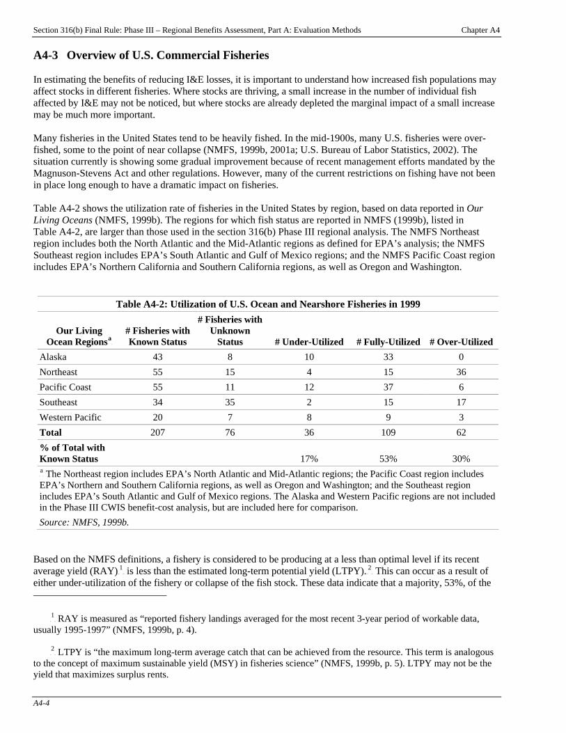
Section 316(b) Final Rule: Phase III – Regional Benefits Assessment, Part A: Evaluation Methods Chapter A4
A4-4
A4-3 Overview of U.S. Commercial Fisheries In estimating the benefits of reducing I&E losses, it is important to understand how increased fish populations may affect stocks in different fisheries. Where stocks are thriving, a small increase in the number of individual fish affected by I&E may not be noticed, but where stocks are already depleted the marginal impact of a small increase may be much more important. Many fisheries in the United States tend to be heavily fished. In the mid-1900s, many U.S. fisheries were over-fished, some to the point of near collapse (NMFS, 1999b, 2001a; U.S. Bureau of Labor Statistics, 2002). The situation currently is showing some gradual improvement because of recent management efforts mandated by the Magnuson-Stevens Act and other regulations. However, many of the current restrictions on fishing have not been in place long enough to have a dramatic impact on fisheries. Table A4-2 shows the utilization rate of fisheries in the United States by region, based on data reported in Our Living Oceans (NMFS, 1999b). The regions for which fish status are reported in NMFS (1999b), listed in Table A4-2, are larger than those used in the section 316(b) Phase III regional analysis. The NMFS Northeast region includes both the North Atlantic and the Mid-Atlantic regions as defined for EPA’s analysis; the NMFS Southeast region includes EPA’s South Atlantic and Gulf of Mexico regions; and the NMFS Pacific Coast region includes EPA’s Northern California and Southern California regions, as well as Oregon and Washington.
Table A4-2: Utilization of U.S. Ocean and Nearshore Fisheries in 1999
Our Living Ocean RegionsP
aP
# Fisheries with Known Status
# Fisheries with Unknown
Status # Under-Utilized # Fully-Utilized # Over-Utilized Alaska 43 8 10 33 0 Northeast 55 15 4 15 36 Pacific Coast 55 11 12 37 6 Southeast 34 35 2 15 17 Western Pacific 20 7 8 9 3 Total 207 76 36 109 62 % of Total with Known Status
17% 53% 30%
P
aP The Northeast region includes EPA’s North Atlantic and Mid-Atlantic regions; the Pacific Coast region includes
EPA’s Northern and Southern California regions, as well as Oregon and Washington; and the Southeast region includes EPA’s South Atlantic and Gulf of Mexico regions. The Alaska and Western Pacific regions are not included in the Phase III CWIS benefit-cost analysis, but are included here for comparison. Source: NMFS, 1999b.
Based on the NMFS definitions, a fishery is considered to be producing at a less than optimal level if its recent average yield (RAY)TPF
1FPT is less than the estimated long-term potential yield (LTPY).TPF
2FPT This can occur as a result of
either under-utilization of the fishery or collapse of the fish stock. These data indicate that a majority, 53%, of the
TP
1PT RAY is measured as “reported fishery landings averaged for the most recent 3-year period of workable data,
usually 1995-1997” (NMFS, 1999b, p. 4).
TP
2PT LTPY is “the maximum long-term average catch that can be achieved from the resource. This term is analogous
to the concept of maximum sustainable yield (MSY) in fisheries science” (NMFS, 1999b, p. 5). LTPY may not be the yield that maximizes surplus rents.
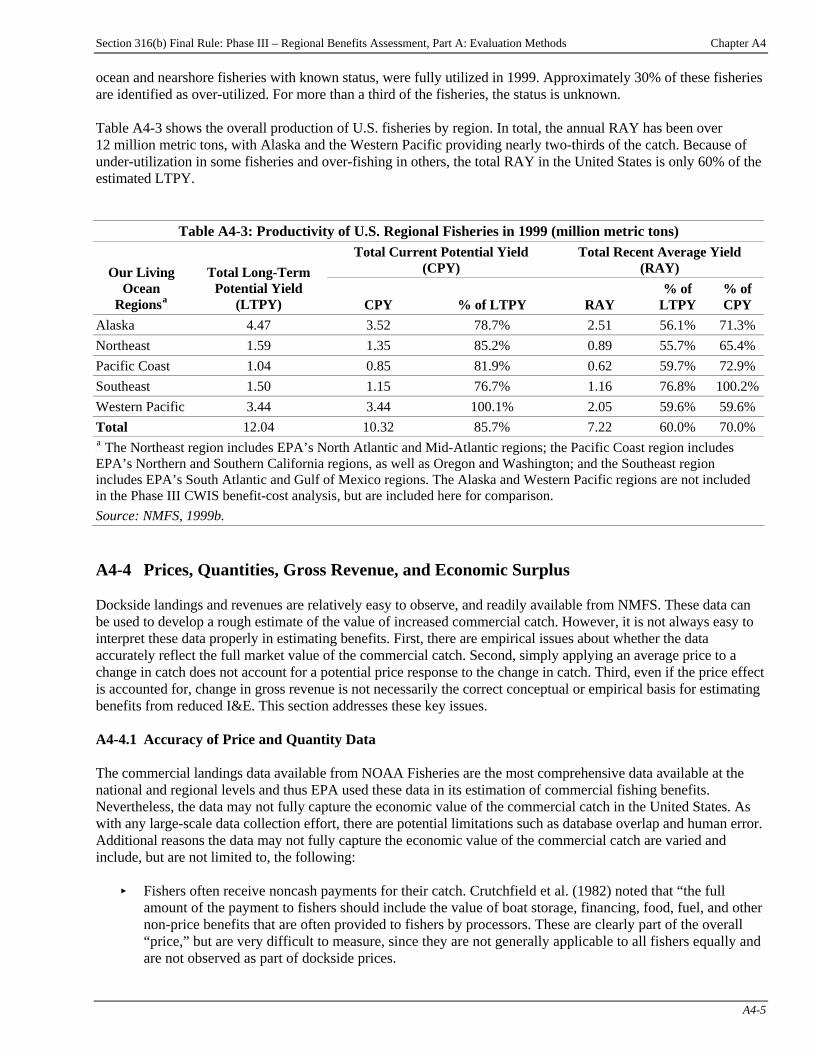
Section 316(b) Final Rule: Phase III – Regional Benefits Assessment, Part A: Evaluation Methods Chapter A4
A4-5
ocean and nearshore fisheries with known status, were fully utilized in 1999. Approximately 30% of these fisheries are identified as over-utilized. For more than a third of the fisheries, the status is unknown. Table A4-3 shows the overall production of U.S. fisheries by region. In total, the annual RAY has been over 12 million metric tons, with Alaska and the Western Pacific providing nearly two-thirds of the catch. Because of under-utilization in some fisheries and over-fishing in others, the total RAY in the United States is only 60% of the estimated LTPY.
Table A4-3: Productivity of U.S. Regional Fisheries in 1999 (million metric tons) Total Current Potential Yield
(CPY) Total Recent Average Yield
(RAY) Our Living Ocean
RegionsP
aP
Total Long-Term Potential Yield
(LTPY) CPY % of LTPY RAY % of
LTPY % of CPY
Alaska 4.47 3.52 78.7% 2.51 56.1% 71.3% Northeast 1.59 1.35 85.2% 0.89 55.7% 65.4% Pacific Coast 1.04 0.85 81.9% 0.62 59.7% 72.9% Southeast 1.50 1.15 76.7% 1.16 76.8% 100.2%Western Pacific 3.44 3.44 100.1% 2.05 59.6% 59.6% Total 12.04 10.32 85.7% 7.22 60.0% 70.0% P
aP The Northeast region includes EPA’s North Atlantic and Mid-Atlantic regions; the Pacific Coast region includes
EPA’s Northern and Southern California regions, as well as Oregon and Washington; and the Southeast region includes EPA’s South Atlantic and Gulf of Mexico regions. The Alaska and Western Pacific regions are not included in the Phase III CWIS benefit-cost analysis, but are included here for comparison. Source: NMFS, 1999b. A4-4 Prices, Quantities, Gross Revenue, and Economic Surplus Dockside landings and revenues are relatively easy to observe, and readily available from NMFS. These data can be used to develop a rough estimate of the value of increased commercial catch. However, it is not always easy to interpret these data properly in estimating benefits. First, there are empirical issues about whether the data accurately reflect the full market value of the commercial catch. Second, simply applying an average price to a change in catch does not account for a potential price response to the change in catch. Third, even if the price effect is accounted for, change in gross revenue is not necessarily the correct conceptual or empirical basis for estimating benefits from reduced I&E. This section addresses these key issues. A4-4.1 Accuracy of Price and Quantity Data The commercial landings data available from NOAA Fisheries are the most comprehensive data available at the national and regional levels and thus EPA used these data in its estimation of commercial fishing benefits. Nevertheless, the data may not fully capture the economic value of the commercial catch in the United States. As with any large-scale data collection effort, there are potential limitations such as database overlap and human error. Additional reasons the data may not fully capture the economic value of the commercial catch are varied and include, but are not limited to, the following:
< Fishers often receive noncash payments for their catch. Crutchfield et al. (1982) noted that “the full amount of the payment to fishers should include the value of boat storage, financing, food, fuel, and other non-price benefits that are often provided to fishers by processors. These are clearly part of the overall “price,” but are very difficult to measure, since they are not generally applicable to all fishers equally and are not observed as part of dockside prices.
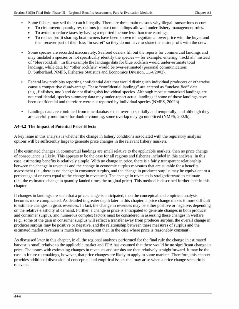
Section 316(b) Final Rule: Phase III – Regional Benefits Assessment, Part A: Evaluation Methods Chapter A4
A4-6
< Some fishers may sell their catch illegally. There are three main reasons why illegal transactions occur: • To circumvent quantity restrictions (quotas) on landings allowed under fishery management rules. • To avoid or reduce taxes by having a reported income less than true earnings. • To reduce profit sharing, boat owners have been known to negotiate a lower price with the buyer and
then recover part of their loss “in secret” so they do not have to share the entire profit with the crew.
< Some species are recorded inaccurately. Seafood dealers fill out the reports for commercial landings and may mislabel a species or not specifically identify the species — for example, entering “rockfish” instead of “blue rockfish.” In this example the landings data for blue rockfish would under-estimate total landings, while data for “other rockfish” would be over-estimated (personal communication; D. Sutherland, NMFS, Fisheries Statistics and Economics Division, 11/4/2002).
< Federal law prohibits reporting confidential data that would distinguish individual producers or otherwise
cause a competitive disadvantage. These “confidential landings” are entered as “unclassified” data (e.g., finfishes, unc.) and do not distinguish individual species. Although most summarized landings are not confidential, species summary data may under-report actual landings if some of those landings have been confidential and therefore were not reported by individual species (NMFS, 2002b).
< Landings data are combined from nine databases that overlap spatially and temporally, and although they
are carefully monitored for double-counting, some overlap may go unnoticed (NMFS, 2002b).
A4-4.2 The Impact of Potential Price Effects A key issue in this analysis is whether the change in fishery conditions associated with the regulatory analysis options will be sufficiently large to generate price changes in the relevant fishery markets. If the estimated changes in commercial landings are small relative to the applicable markets, then no price change of consequence is likely. This appears to be the case for all regions and fisheries included in this analysis. In this case, estimating benefits is relatively simple. With no change in price, there is a fairly transparent relationship between the change in revenues and the change in economic surplus measures that are suitable for a benefits assessment (i.e., there is no change in consumer surplus, and the change in producer surplus may be equivalent to a percentage of or even equal to the change in revenues). The change in revenues is straightforward to estimate (i.e., the estimated change in quantity landed times the original price). This method is described further later in this chapter. If changes in landings are such that a price change is anticipated, then the conceptual and empirical analysis becomes more complicated. As detailed in greater depth later in this chapter, a price change makes it more difficult to estimate changes in gross revenues. In fact, the change in revenues may be either positive or negative, depending on the relative elasticity of demand. Further, a change in price is anticipated to generate changes in both producer and consumer surplus, and numerous complex factors must be considered in assessing these changes in welfare (e.g., some of the gain in consumer surplus will reflect a transfer away from producer surplus, the overall change in producer surplus may be positive or negative, and the relationship between these measures of surplus and the estimated market revenues is much less transparent than in the case where price is reasonably constant). As discussed later in this chapter, in all the regional analyses performed for the final rule the change in estimated harvest is small relative to the applicable market and EPA has assumed that there would be no significant change in price. The issues with estimating changes in revenues and surplus are then relatively straightforward. It may be the case in future rulemakings, however, that price changes are likely to apply in some markets. Therefore, this chapter provides additional discussion of conceptual and empirical issues that may arise when a price change scenario is relevant.
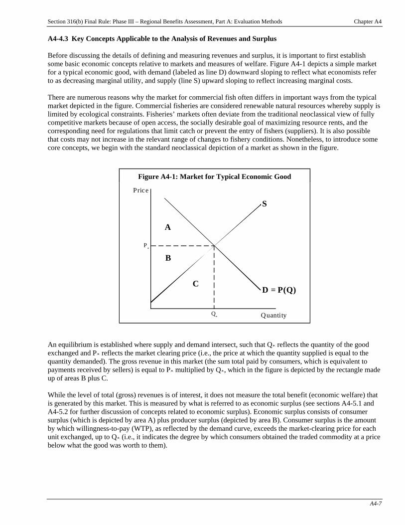
Section 316(b) Final Rule: Phase III – Regional Benefits Assessment, Part A: Evaluation Methods Chapter A4
A4-7
A4-4.3 Key Concepts Applicable to the Analysis of Revenues and Surplus Before discussing the details of defining and measuring revenues and surplus, it is important to first establish some basic economic concepts relative to markets and measures of welfare. Figure A4-1 depicts a simple market for a typical economic good, with demand (labeled as line D) downward sloping to reflect what economists refer to as decreasing marginal utility, and supply (line S) upward sloping to reflect increasing marginal costs. There are numerous reasons why the market for commercial fish often differs in important ways from the typical market depicted in the figure. Commercial fisheries are considered renewable natural resources whereby supply is limited by ecological constraints. Fisheries’ markets often deviate from the traditional neoclassical view of fully competitive markets because of open access, the socially desirable goal of maximizing resource rents, and the corresponding need for regulations that limit catch or prevent the entry of fishers (suppliers). It is also possible that costs may not increase in the relevant range of changes to fishery conditions. Nonetheless, to introduce some core concepts, we begin with the standard neoclassical depiction of a market as shown in the figure.
Figure A4-1: Market for Typical Economic Good
Price
Quantity
S
D = P(Q)
Q*
P*
C
B
A
An equilibrium is established where supply and demand intersect, such that QB*B reflects the quantity of the good exchanged and PB*B reflects the market clearing price (i.e., the price at which the quantity supplied is equal to the quantity demanded). The gross revenue in this market (the sum total paid by consumers, which is equivalent to payments received by sellers) is equal to PB*B multiplied by QB*B, which in the figure is depicted by the rectangle made up of areas B plus C. While the level of total (gross) revenues is of interest, it does not measure the total benefit (economic welfare) that is generated by this market. This is measured by what is referred to as economic surplus (see sections A4-5.1 and A4-5.2 for further discussion of concepts related to economic surplus). Economic surplus consists of consumer surplus (which is depicted by area A) plus producer surplus (depicted by area B). Consumer surplus is the amount by which willingness-to-pay (WTP), as reflected by the demand curve, exceeds the market-clearing price for each unit exchanged, up to QB*B (i.e., it indicates the degree by which consumers obtained the traded commodity at a price below what the good was worth to them).

Section 316(b) Final Rule: Phase III – Regional Benefits Assessment, Part A: Evaluation Methods Chapter A4
A4-8
Likewise, producer surplus reflects the extent to which suppliers realized revenues above and beyond the marginal cost of producing some of the units (up to QB*B). Beyond QB*B, there is neither additional consumer nor producer surplus to be gained — at the margin, all the surplus has been extracted and no additional surplus will be gained by adding more output to the market. Now, suppose there is a change that increases the amount of a key input to production, such that the more bountiful input is now available at a lower cost to suppliers than before. For example, an increase in the number of locally harvestable fish makes it easier, and thus less costly, to catch a given number of fish. This could result in an outward shift in supply (a decrease in the marginal cost of producing any given quantity of the good). This is depicted in Figure A4-2, where supply shifts from SB0B to SB1B. With the increased supply, a new market clearing price emerges at PB1B (which is lower than the original PB*B), and the quantity exchanged increases from QB*B to QB1B.
Figure A4-2: Increased Supply in Typical Economic Market
Price
Quantity
S0
S1
D
G
Q1
Q*
Z
Y
D
F
P*
P1
E
B
A
X
C
These changes in the quantity exchanged and the market-clearing price make it somewhat complex to envision how (and by how much) gross revenues and economic surplus measures may change as a consequence of the shift in supply. Using Figure A4-2 as a guide:
< Under the original supply conditions (SB0B) consumer surplus had been area A, but it has now increased to A + B + C + D. Therefore, consumer surplus has increased by an amount depicted by areas B + C + D.
< Producer surplus had been area B + E before the supply shift, but becomes E + F + G after the shift in
supply. Hence the change in producer surplus is depicted as areas F + G - B. • Note that area B is subtracted from producer surplus but added to consumer surplus — i.e., it
represents a transfer of surplus from producers to consumers when supply shifts outward and prices decline.
• Also note that consumer surplus has increased by more than the transfer of area B from producers; the additional consumer surplus (above and beyond the transfer) is depicted by the amount C + D.
• Finally, note that the change in producer surplus might be positive or negative, depending on whether the addition of F + G outweighs the loss of B (assuming the supply curves are parallel).
< The total change in economic surplus (consumer plus producer surplus) therefore equals C + D + F + G.
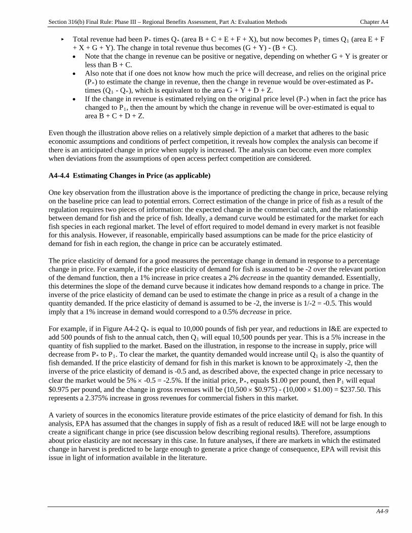
Section 316(b) Final Rule: Phase III – Regional Benefits Assessment, Part A: Evaluation Methods Chapter A4
A4-9
< Total revenue had been PB*B times QB*B (area B + C + E + F + X), but now becomes PB1B times QB1B (area E + F + X + G + Y). The change in total revenue thus becomes (G + Y) - (B + C). • Note that the change in revenue can be positive or negative, depending on whether G + Y is greater or
less than B + C. • Also note that if one does not know how much the price will decrease, and relies on the original price
(PB*B) to estimate the change in revenue, then the change in revenue would be over-estimated as PB*B times (QB1B - QB*B), which is equivalent to the area G + Y + D + Z.
• If the change in revenue is estimated relying on the original price level (PB*B) when in fact the price has changed to PB1B, then the amount by which the change in revenue will be over-estimated is equal to area B + C + D + Z.
Even though the illustration above relies on a relatively simple depiction of a market that adheres to the basic economic assumptions and conditions of perfect competition, it reveals how complex the analysis can become if there is an anticipated change in price when supply is increased. The analysis can become even more complex when deviations from the assumptions of open access perfect competition are considered. A4-4.4 Estimating Changes in Price (as applicable) One key observation from the illustration above is the importance of predicting the change in price, because relying on the baseline price can lead to potential errors. Correct estimation of the change in price of fish as a result of the regulation requires two pieces of information: the expected change in the commercial catch, and the relationship between demand for fish and the price of fish. Ideally, a demand curve would be estimated for the market for each fish species in each regional market. The level of effort required to model demand in every market is not feasible for this analysis. However, if reasonable, empirically based assumptions can be made for the price elasticity of demand for fish in each region, the change in price can be accurately estimated. The price elasticity of demand for a good measures the percentage change in demand in response to a percentage change in price. For example, if the price elasticity of demand for fish is assumed to be -2 over the relevant portion of the demand function, then a 1% increase in price creates a 2% decrease in the quantity demanded. Essentially, this determines the slope of the demand curve because it indicates how demand responds to a change in price. The inverse of the price elasticity of demand can be used to estimate the change in price as a result of a change in the quantity demanded. If the price elasticity of demand is assumed to be -2, the inverse is 1/-2 = -0.5. This would imply that a 1% increase in demand would correspond to a 0.5% decrease in price. For example, if in Figure A4-2 QB*B is equal to 10,000 pounds of fish per year, and reductions in I&E are expected to add 500 pounds of fish to the annual catch, then QB1B will equal 10,500 pounds per year. This is a 5% increase in the quantity of fish supplied to the market. Based on the illustration, in response to the increase in supply, price will decrease from PB*B to PB1B. To clear the market, the quantity demanded would increase until QB1B is also the quantity of fish demanded. If the price elasticity of demand for fish in this market is known to be approximately -2, then the inverse of the price elasticity of demand is -0.5 and, as described above, the expected change in price necessary to clear the market would be 5% × -0.5 = -2.5%. If the initial price, PB*B, equals $1.00 per pound, then PB1B will equal $0.975 per pound, and the change in gross revenues will be (10,500 × $0.975) - (10,000 × $1.00) = $237.50. This represents a 2.375% increase in gross revenues for commercial fishers in this market. A variety of sources in the economics literature provide estimates of the price elasticity of demand for fish. In this analysis, EPA has assumed that the changes in supply of fish as a result of reduced I&E will not be large enough to create a significant change in price (see discussion below describing regional results). Therefore, assumptions about price elasticity are not necessary in this case. In future analyses, if there are markets in which the estimated change in harvest is predicted to be large enough to generate a price change of consequence, EPA will revisit this issue in light of information available in the literature.
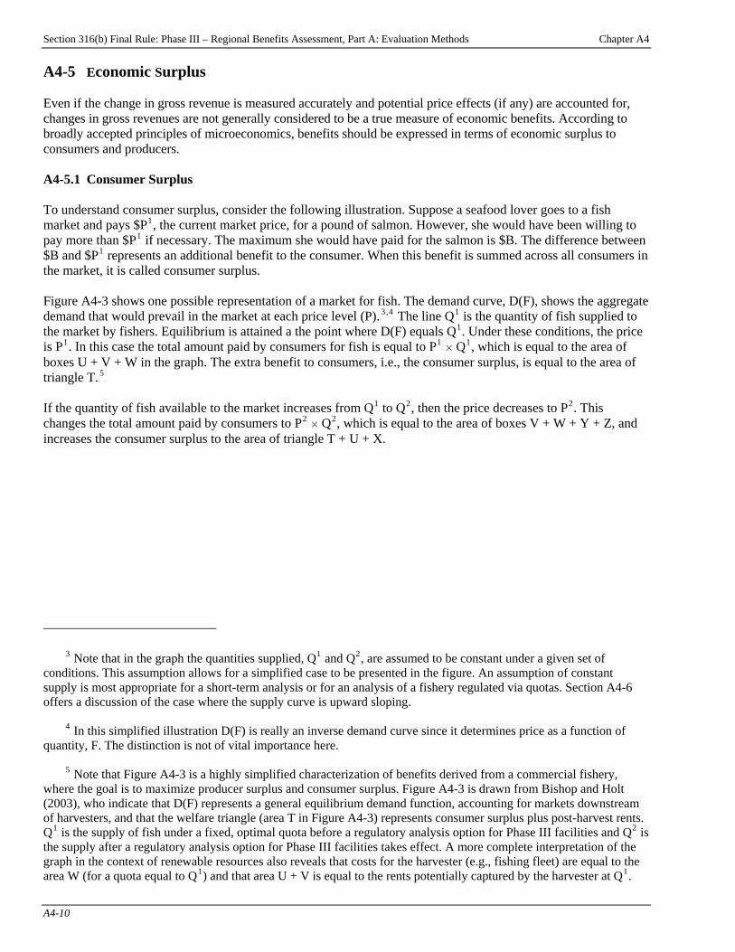
Section 316(b) Final Rule: Phase III – Regional Benefits Assessment, Part A: Evaluation Methods Chapter A4
A4-10
A4-5 Economic Surplus Even if the change in gross revenue is measured accurately and potential price effects (if any) are accounted for, changes in gross revenues are not generally considered to be a true measure of economic benefits. According to broadly accepted principles of microeconomics, benefits should be expressed in terms of economic surplus to consumers and producers. A4-5.1 Consumer Surplus To understand consumer surplus, consider the following illustration. Suppose a seafood lover goes to a fish market and pays $PP
1P, the current market price, for a pound of salmon. However, she would have been willing to
pay more than $PP
1P if necessary. The maximum she would have paid for the salmon is $B. The difference between
$B and $PP
1P represents an additional benefit to the consumer. When this benefit is summed across all consumers in
the market, it is called consumer surplus. Figure A4-3 shows one possible representation of a market for fish. The demand curve, D(F), shows the aggregate demand that would prevail in the market at each price level (P).PF
3F
,F
4FP The line QP
1P is the quantity of fish supplied to
the market by fishers. Equilibrium is attained a the point where D(F) equals QP
1P. Under these conditions, the price
is PP
1P. In this case the total amount paid by consumers for fish is equal to PP
1P H QP
1P, which is equal to the area of
boxes U + V + W in the graph. The extra benefit to consumers, i.e., the consumer surplus, is equal to the area of triangle T.PF
5FP
If the quantity of fish available to the market increases from QP
1P to QP
2P, then the price decreases to PP
2P. This
changes the total amount paid by consumers to PP
2P H QP
2P, which is equal to the area of boxes V + W + Y + Z, and
increases the consumer surplus to the area of triangle T + U + X.
P
3P Note that in the graph the quantities supplied, QP
1P and QP
2P, are assumed to be constant under a given set of
conditions. This assumption allows for a simplified case to be presented in the figure. An assumption of constant supply is most appropriate for a short-term analysis or for an analysis of a fishery regulated via quotas. Section A4-6 offers a discussion of the case where the supply curve is upward sloping.
P
4P In this simplified illustration D(F) is really an inverse demand curve since it determines price as a function of
quantity, F. The distinction is not of vital importance here.
P
5P Note that Figure A4-3 is a highly simplified characterization of benefits derived from a commercial fishery,
where the goal is to maximize producer surplus and consumer surplus. Figure A4-3 is drawn from Bishop and Holt (2003), who indicate that D(F) represents a general equilibrium demand function, accounting for markets downstream of harvesters, and that the welfare triangle (area T in Figure A4-3) represents consumer surplus plus post-harvest rents. QP
1P is the supply of fish under a fixed, optimal quota before a regulatory analysis option for Phase III facilities and QP
2P is
the supply after a regulatory analysis option for Phase III facilities takes effect. A more complete interpretation of the graph in the context of renewable resources also reveals that costs for the harvester (e.g., fishing fleet) are equal to the area W (for a quota equal to QP
1P) and that area U + V is equal to the rents potentially captured by the harvester at QP
1P.
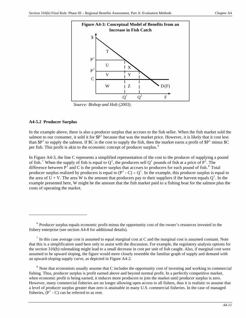
Section 316(b) Final Rule: Phase III – Regional Benefits Assessment, Part A: Evaluation Methods Chapter A4
A4-11
Figure A4-3: Conceptual Model of Benefits from an Increase in Fish Catch
$
P1
C
T
U
V
W
XY
Z D
F
P2
Q1 Q2
(F)
Source: Bishop and Holt (2003).
A4-5.2 Producer Surplus In the example above, there is also a producer surplus that accrues to the fish seller. When the fish market sold the salmon to our consumer, it sold it for $PP
1P because that was the market price. However, it is likely that it cost less
than $PP
1P to supply the salmon. If $C is the cost to supply the fish, then the market earns a profit of $PP
1P minus $C
per fish. This profit is akin to the economic concept of producer surplus.PF
6FP
In Figure A4-3, the line C represents a simplified representation of the cost to the producer of supplying a pound of fish.PF
7FP When the supply of fish is equal to QP
1P, the producers sell QP
1P pounds of fish at a price of PP
1P. The
difference between PP
1P and C is the producer surplus that accrues to producers for each pound of fish.PF
8FP Total
producer surplus realized by producers is equal to (PP
1P - C) H QP
1P. In the example, this producer surplus is equal to
the area of U + V. The area W is the amount that producers pay to their suppliers if the harvest equals QP
1P. In the
example presented here, W might be the amount that the fish market paid to a fishing boat for the salmon plus the costs of operating the market.
P
6P Producer surplus equals economic profit minus the opportunity cost of the owner’s resources invested in the
fishery enterprise (see section A4-8 for additional details).
P
7P In this case average cost is assumed to equal marginal cost at C and the marginal cost is assumed constant. Note
that this is a simplification used here only to assist with the discussion. For example, the regulatory analysis options for the section 316(b) rulemaking might lead to a small decrease in cost per unit of fish caught. Also, if marginal cost were assumed to be upward sloping, the figure would more closely resemble the familiar graph of supply and demand with an upward-sloping supply curve, as depicted in Figure A4-2.
P
8P Note that economists usually assume that C includes the opportunity cost of investing and working in commercial
fishing. Thus, producer surplus is profit earned above and beyond normal profit. In a perfectly competitive market, when economic profit is being earned, it induces more producers to join the market until producer surplus is zero. However, many commercial fisheries are no longer allowing open access to all fishers, thus it is realistic to assume that a level of producer surplus greater than zero is attainable in many U.S. commercial fisheries. In the case of managed fisheries, (PP
1P - C) can be referred to as rent.
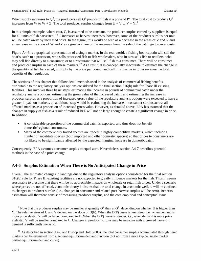
Section 316(b) Final Rule: Phase III – Regional Benefits Assessment, Part A: Evaluation Methods Chapter A4
A4-12
When supply increases to QP
2P, the producers sell QP
2P pounds of fish at a price of PP
2P. The total cost to produce QP
2P
increases from W to W + Z. The total producer surplus changes from U + V to V + Y.PF
9FP
In this simple example, where cost, C, is assumed to be constant, the producer surplus earned by suppliers is equal for all units of fish harvested. If C increases as harvest increases, however, some of the producer surplus per unit will be eaten away by increased costs. In the figure, this would be seen as a decrease in the areas of V and Y and an increase in the areas of W and Z as a greater share of the revenues from the sale of the catch go to cover costs. Figure A4-3 is a graphical representation of a single market. In the real world, a fishing boat captain will sell the boat’s catch to a processor, who sells processed fish to fish wholesalers, who in turn sells fish to retailers, who may sell fish directly to a consumer, or to a restaurant that will sell fish to a consumer. There will be consumer and producer surplus in each of these markets.PF
10FP As a result, it is conceptually inaccurate to estimate the change in
the quantity of fish harvested, multiply by the price per pound, and call this change in gross revenue the total benefits of the regulation. The sections of this chapter that follow detail methods used in the analysis of commercial fishing benefits attributable to the regulatory analysis options considered for the final section 316(b) rule for Phase III existing facilities. This involves three basic steps: estimating the increase in pounds of commercial catch under the regulatory analysis options, estimating the gross value of the increased catch, and estimating the increase in producer surplus as a proportion of increased gross value. If the regulatory analysis options were expected to have a greater impact on markets, an additional step would be estimating the increase in consumer surplus across all affected markets as a proportion of increased gross value. However, as detailed above, EPA has assumed that the changes in supply of fish as a result of reduced I&E will not be large enough to create a significant change in price. In addition:
< A considerable proportion of the commercial catch is exported, and thus does not benefit domestic/regional consumers.
< Many of the commercially traded species are traded in highly competitive markets, which include a number of substitute species (both imported and other domestic species) so that prices to consumers are not likely to be significantly affected by the expected marginal increase in domestic catch.
Consequently, EPA assumes consumer surplus to equal zero. Nevertheless, section A4-7 describes potential methods in the case of a price change. A4-6 Surplus Estimation When There is No Anticipated Change in Price Overall, the estimated changes in landings due to the regulatory analysis options considered for the final section 316(b) rule for Phase III existing facilities are not expected to greatly influence markets for the fish. Thus, it seems reasonable to presume that there will be no appreciable impacts on wholesale or retail fish prices. Under a scenario where prices are not affected, economic theory indicates that the total change in economic welfare will be confined to changes in producer surplus (i.e., changes in consumer and related post-harvest surplus will be zero). Benefits estimation will therefore consist of measuring producer surplus, and the core empirical and conceptual issue
P
9P Note that the producer surplus may be smaller at quantity QP
2P than at QP
1P, depending on whether U is bigger than
Y. The relative sizes of U and Y depend on the slope of D(F). When the D(F) curve is less steep, i.e., when demand is more price elastic, Y will be larger compared to U. When the D(F) curve is steeper, i.e., when demand is more price inelastic, Y will be smaller compared to U. Changes in producer surplus may be negative with increased harvest if demand is sufficiently inelastic.
P
10P As described in section A4-8 and Bishop and Holt (2003), the total consumer surplus accumulated through tiered
markets can be estimated from a general equilibrium demand function (but not from a more typical single market partial equilibrium demand curve).

Section 316(b) Final Rule: Phase III – Regional Benefits Assessment, Part A: Evaluation Methods Chapter A4
A4-13
becomes determining the relationship between increases in gross revenues and changes in producer surplus, when prices remain constant. A4-6.1 Producer Surplus as a Percentage of Gross Revenues: Assuming No Change in Prices Given the potential for increases in producer surplus for the harvest sector (including rents to harvesters) under conditions where fish prices do not change, EPA has estimated producer surplus as a constant fraction of the change in gross revenue. There are at least two relevant cases to consider: the case of unregulated fisheries, and the case of fisheries that are regulated with quotas or restrictive permits. A4-6.2 Unregulated Fisheries In an unregulated fishery, a reduction in I&E that leads to an increase in the stock of fish will decrease the marginal cost of catching more fish. This makes it possible for fishers to earn economic rents, and for producer surplus to increase. According to basic microeconomic principles, in a competitive market economic rents will attract additional fishing effort in one of two ways: either existing fishers will exert greater effort or new fishers will enter the market (or both). In either case, fishing effort theoretically will increase until a new equilibrium is reached where economic rents are equal to zero. In this case, there may be economic benefits to commercial fishers in the short term, but in the long run producer surplus will be zero. Thus, in an unregulated fishery economic theory suggests that the long-run change in producer surplus will be 0% of the change in gross revenues. A4-6.3 Regulated Fisheries Fishery regulations seek to create sustainable harvests that maximize resource rents. In a regulated fishery, reduced I&E that increases the number of fish available to harvest, may lead to increases in harvest, if regulations are relaxed to allow for greater harvest. In this case, unlike the open access case, there will be lasting benefits to commercial fishers. As an example, assume that quotas are the regulatory instrument, that quotas increase (from QB0B to QB1B) in response to reduced I&E, and that the supply curve (as represented by a marginal cost curve) shifts as a result of increased stock (from SB0B to SB1B). Then, we can relate the change in producer surplus to the change in gross revenue, as illustrated in Figure A4-4. Before the increase in stock and change in quota, producer surplus is equal to area A. After the increase in stock and change in quota, producer surplus is equal to area (A + B + D + E). The change in producer surplus resulting from the increased quota is therefore equal to area (B + D + E).
Figure A4-4: Surplus in a Regulated Fishery Where Price is Constant
Price
Quantity
A
B
CF
E
DP
S0
S1
D
Q1
Q0
MC0
MC1
Section 316(b) Final Rule: Phase III – Regional Benefits Assessment, Part A: Evaluation Methods Chapter A4
A4-14
Before the increase in stock and change in quota, total revenue is equal to area (A + B + C). After the increase in stock and change in quota, total revenue is equal to area (A + B + C + D + E + F). The change in total revenue resulting from the increased quota is therefore equal to area (D + E + F). Therefore, the relationship between the change in producer surplus and the change in total revenue depends on the relative magnitudes of areas B and F. Three scenarios illustrate how the change in total revenue may over- or under-estimate the change in producer surplus:
1. If B < F, then the change in revenue over-estimates the change in producer surplus. 2. If B = F, then the change in revenue approximates the change in producer surplus. 3. If B > F, then the change in revenue underestimates the change in producer surplus.
Note that if the first scenario prevails, then some fraction of gross revenue may be more suitable as a reliable proxy for change in producer surplus when price is assumed constant. If the marginal cost of supplying the extra fish at the higher quota, QB1B, is minimal or close to zero, then the second or third scenarios are likely, and 100% or more of the change in revenue may serve as a reliable proxy for the change in producer surplus. A4-6.4 Conclusions on Surplus When No Change in Price is Anticipated Various scenarios may arise when fishery conditions improve such that supply increases without generating a price change of consequence. When prices do not change, there is no anticipated change in post-harvest surplus to consumers or other post harvest entities, because a reduction in price is required to generate such changes. Hence, under these conditions, the change in economic welfare is limited to changes in producer surplus. As shown in the previous section, estimates of changes in dockside revenues become, under some scenarios, equivalent to the change in producer surplus. Hence, the change in gross revenues can be used as a proxy to estimate the change in producer surplus for the regional analyses.TPF
11FPT EPA also recognizes that under some of the
possible scenarios that may arise when there is a quota-governed market, the full change in revenues (as estimated through a projected change in landings but no price change) might overstate the change in producer surplus. However, if dockside prices and/or dockside landings (quantities) are understated — as may often be the case — then the change in surplus will be understated in most scenarios when approximated by the estimated change in gross revenues. EPA’s analysis of commercial fishery benefits relies on the premise that the change in producer surplus is a fraction of the projected change in revenues. EPA estimated a species- and region-specific fraction, providing a range of 0% to 84%. The lower estimate of 0% represents the case of an unregulated fishery, as well as is the lower bound identified in the literature. This is described in greater detail in section A4-10. A4-7 Surplus Estimation Under Scenarios in Which Price May Change In the preceding section, the discussion was limited to cases in which no notable change in price was anticipated. These scenarios appear reasonable for very small improvements in fishery conditions, which is relevant for the regional analyses. If the estimated impacts were larger, as may be the case in other analyses, it may be inappropriate to assume that there will be no price effects in any commercial fishery markets. This section discusses the conceptual and empirical basis for estimating economic surplus (i.e., benefits) in instances where price changes are more likely to arise.
TP
11PT This is consistent with EPA’s guidelines (U.S. EPA, 2000a). The guidelines describe options for estimating
ecological benefits for fisheries, and note that “if changes in service flows are small, current market prices can be used as a proxy for expected benefit . . . a change in the commercial fish catch might be valued using the market price for the affected species” (p. 98).
Section 316(b) Final Rule: Phase III – Regional Benefits Assessment, Part A: Evaluation Methods Chapter A4
A4-15
A4-7.1 Neoclassical Economic Perspective on the Market and Economic Welfare Figure A4-2 and section A4-4.3 described the standard, neoclassical economic depiction of a market, with demand downward sloping and supply upward sloping to reflect increasing marginal costs. There are several reasons why this neoclassical depiction may not be directly applicable to the commercial fisheries market, as discussed later in this chapter. But for the moment, Figure A4-2 and the related discussion provide a useful starting point for considering how the measures of economic benefit — the sum of producer and consumer surplus — might change due to a policy that shifts the supply curve outward from SB0B to SB1B. As noted previously, a portion of the gain in consumer surplus (represented by area B in Figure A4-2) is, in effect, a transfer from producer surplus. Any empirical effort to estimate changes in surplus needs to ensure that if change in total surplus is included in the estimate of post-harvest surplus, then the producer surplus estimate should be made net of this quantity to ensure no double counting.TPF
12FPT
Other noteworthy observations, as discussed in section 4-4.3, are that, under some circumstances, the change in revenues may be zero or even negative and the change in producer surplus can be positive or negative. Even with the transfer of area B from producer to consumer surplus, there are still positive net gains in producer surplus if F + G > B. A4-7.2 Issues in Estimating Changes in Welfare The discussion above regarding welfare measures — and how they change with shifts in supply within the neoclassical framework — is fairly complex, even in its simplest form. To estimate such changes in welfare as may arise from the regulatory analysis options for the section 316(b) regulation, the problem becomes even more complicated. Some of the empirical and conceptual complications are discussed below. In an expedited regulatory analysis that must cover a broad range of fish species across locations and fishery markets that span the nation, EPA must rely on readily applicable generalized approaches (rather than more detailed, market-specific assessments) to estimate changes in welfare. Hence, as noted earlier in this chapter, EPA must rely on readily estimated changes in gross revenues and from there infer potential changes in post-harvest (consumer) and producer surplus. Also, there are several issues associated with how to implement an expedited approach. First, there is the issue of how to estimate the change in gross revenues. These changes in revenues are the product of the projected changes in fish harvests times observed baseline market prices. Thus, EPA can readily obtain an estimate comparable to the area Y + Z + A + B in Figure A4-5. This is the approach contemplated by the Agency for this rulemaking to handle the case in which prices change. To more suitably capture the impact of a price change, in future analyses EPA may attempt to apply an applicable estimate of price elasticity to obtain an estimate that better reflects the true measure of the change in gross revenues (i.e., areas Y + Z - U - V in Figure A4-5). Second, there is the issue of how to infer changes in post-harvest (consumer) surplus based on changes in revenues. The approach described by Bishop and Holt (2003), described in greater detail in section A4-8, is specifically designed to examine this issue. Their empirical research — limited to date to some regions and fisheries (e.g., the Great Lakes) — suggests that the changes in post-harvest surplus may be approximated by the estimated change in
TP
12PT Later in this chapter an approach developed by Bishop and Holt (2003) to estimating post-harvest surplus as
depicted by areas B + C + D is described. Also, note that if the fishery in question is being conducted under open access, this means that rents to the resource are zero or very close it. Suppose furthermore that in this particular case other rents (e.g., rents to scarce fishing skills and knowledge) are also zero. Now suppose that section 316(b) regulatory analysis options are imposed on Phase III facilities, causing an increase in the harvest of fish. The catch increases, but any effects on rents to the resource are dissipated by entry. The effect of the regulatory analysis options is to increase consumer surplus by an amount comparable to areas U + V + B in Figure A4-5, but there is no offsetting decline in producer surplus because there was no producer surplus in the first place.

Section 316(b) Final Rule: Phase III – Regional Benefits Assessment, Part A: Evaluation Methods Chapter A4
A4-16
gross revenues (where the latter is based on holding price constant at baseline levels). This method may also be revisited by EPA in future analyses. Third, there are a series of issues associated with how to estimate the change in producer surplus. Estimating the change in producer surplus under a scenario in which market forces produce a price change is a challenging exercise for a number of reasons, including:
< Many commercial fishery markets do not adhere to the usual assumptions of the neoclassical model because of regulations that establish harvest quotas and/or restrict entry through a permit system. These regulations typically are instituted to protect stocks that have been or are at risk of being over-fished. There also may be nonregulatory barriers to entry that affect this market, such as the high fixed costs and specialized knowledge and skills required to effectively compete in some fisheries.
< Barriers to entry, regardless of the source, can have a profound impact on the economic welfare analysis.
For example, the neoclassical model of open access would have rents driven to zero, but it is more likely in regulated markets (or a nonregulated market with economic barriers to entry) that there are positive rents accruing from the fishery resource (not to mention rents that accrue as well to specialized fishing skills and knowledge).TPF
13FPT
< Empirical evidence regarding the absolute magnitude of producer surplus is limited (especially for
inferring a relationship with gross revenues). However the approach described earlier succeeded in assessing a region and species-specific proxy for a relationship between producer surplus and gross revenue. The proxy is based on a ratio between normal profits and gross revenue and is called the net benefits ratio (NBRatio). However, interpreting the assessed ratio properly is challenging, for a number of reasons: • Available empirical data pertain to average producer surplus, and EPA’s regulatory analysis must
instead address changes in producer surplus at the margin. • The portion of producer surplus that is transferred to consumers when there is a price reduction
(represented by area U in Figure A4-5) should not be double-counted if it is captured in the estimate of post-harvest surplus and also in the estimated change in producer surplus. Since area U is included in the Bishop-Holt analysis of changes in post-harvest surplus, one needs to ensure that area U is not included in (e.g., has been netted out of) the applicable estimate of the change in producer surplus.
• The estimated empirical relationship between normal profits and gross revenue needs to be adjusted downwards to depict accurately the relationship between producer surplus and gross revenue. Limited empirical evidence is available for such an adjustment, but seems to point to a range between 0.4 and 2.6% (U.S. EPA, 2004e).
It is important to address these issues here because of the manner in which the departure from the neoclassical model affects the interpretation of estimates of average producer surplus relative to changes expected at the margin. For example, marginal costs (MC) for commercial fishers may be minimal for a small increase in landings arising from a small increase in harvestable fish — for small increases in numbers of fish suitable for harvest in an area, small increases in harvest are likely to be realized with minimal added operating expense (i.e., MC at or near zero). This might arise where the fishers fill their quotas more easily, or exert essentially the same level of effort but come back with a few more fish. Where fishing effort and hence fishing costs would not change much, benefits (producer surplus) would equal the change in total revenue or be very close to it. For larger changes, marginal and average costs could shift down.
TP
13PT Given the highly regulated nature of many fisheries today, a wide range of producer effects is conceivable. Even
where revenues decline with a reduction in price, producer surplus could increase despite the loss in revenues. This could occur if the effect on price is relatively small and the effect on costs and revenues is relatively large. The only way to know for sure is to examine producer effects in specific cases or do a benefit transfer exercise using experience in real world fisheries as a guide. Simple approaches (e.g., assuming that there is no consumer surplus because of offsetting producer effects) are not satisfactory if there are changes in prices.

Section 316(b) Final Rule: Phase III – Regional Benefits Assessment, Part A: Evaluation Methods Chapter A4
A4-17
This has implications for interpreting the estimated NBRatios. The standard neoclassical model assumes increasing MC in the relevant range, so that producer surplus approaches zero with additional increments in landings. But for the type of situation that applies to section 316(b) — i.e., with a small change in the harvestable number of fish — and given the nature of the commercial fishery (e.g., high barriers to entry due to quotas or high fixed costs), the context is likely to reflect a situation in which costs decrease (e.g., a shift downward in MC, and perhaps MC that are at or near zero). If so, then the argument that the average estimate for producer surplus overstates the marginal value does not hold (in fact, the opposite may be true — average surplus could be less than producer surplus at the margin). A4-8 Estimating Post-Harvest Economic Surplus in Tiered Markets Producer surplus provides an estimate of the benefits to commercial fishers, but significant benefits can also be expected to accrue to final consumers of fish and to commercial consumers (including processors, wholesalers, retailers, and middlemen) if the projected increase in catches is accompanied by a reduction in price. These benefits can be expected to flow through the tiered commercial fishery market (as described in section A4-1 and in Bishop and Holt, 2003). Bishop and Holt (2003) develop an inverse demand model of six Great Lakes fisheries that they use to estimate changes in welfare as a result of changes in the level of commercial harvest. This flexible model can be used to estimate welfare changes under a variety of conditions in the fishery. It takes as an input the expected change in harvest and baseline gross revenues, and provides as outputs the expected change in gross revenues and change in total compensating variation (CV). CV is the change in income that would be necessary to make consumers’ total utility the same as it was before the reduction in I&E losses resulting from the regulatory analysis options for the final section 316(b) rule for Phase III existing facilities. This is analogous to a measure of willingness to accept compensation in order to forgo the improvement. Conceptually, CV is a measure of welfare similar to consumer surplus. The key difference is that consumer surplus is calculated using the familiar demand function (or curve), which defines the quantity demanded as a function of price and income (in the simple example, Figures A4-1 and A4-2, income is assumed to be constant). CV, on the other hand, is calculated using a compensated demand function, which defines the quantity demanded as a function of price and utility. While consumer surplus and CV are generally very similar welfare measures, CV is considered to be the true measure of benefits (i.e., a more consistent indicator of utility), and consumer surplus is an approximation. The distinction between the two is a subtle point in welfare economics; the exact details are not crucial to the analysis.TPF
14FPT
The key point to note is that estimates of CV from the Holt-Bishop model capture the benefits to final consumers and commercial consumers throughout the various markets in which fish are bought and resold for a given level of harvest. The model output provides a convenient way to estimate the benefits of an increase in harvest as a percentage of gross revenues, and thus a tractable way to estimate the benefits of increased catch that do not accrue to the primary producers.TPF
15FPT See Holt and Bishop (2002) for further detail on the model.
Based on comments received on the commercial benefits analysis for the final Phase II rule, EPA worked with Dr. Bishop to re-assess the suitability of using the results from Holt and Bishop (2002) in a benefit transfer. EPA determined that the magnitude of the changes in commercial catch modeled in the Holt and Bishop paper is, in most cases, larger than the magnitude of the expected changes as a result of the Phase II and Phase III regulations,
TP
14PT For a more detailed discussion of the difference in consumer surplus and CV, the reader is referred to in Varian
(1992, Chapters 7 and 9) or any graduate-level microeconomics text.
TP
15PT Bishop and Holt do not estimate changes in producer surplus, and indicate such changes need to be estimated
separately and then combined with post-harvest consumer surplus results.
Section 316(b) Final Rule: Phase III – Regional Benefits Assessment, Part A: Evaluation Methods Chapter A4
A4-18
and thus the benefits may be quite different. To address this issue, Bishop and Holt (2003) explore the impacts on surplus measures for more moderate changes in fishery conditions, by reestimating their Great Lakes model, relating economic surplus to levels of gross revenues. In this more recent work, Bishop and Holt (2003) observe that, as a general rule of thumb, based on their analysis of the Great Lakes fisheries, the change in CV as a percentage of the change in gross revenues is more or less linearly related to the change in catch. In other words, 10% increase in catch as a result of the regulatory analysis options for Phase III facilities would be expected to produce an increase in CV equal to approximately 10% of the change in gross revenues. As an example, if the regulatory analysis option for Phase III facilities increases the catch of a species by 10% and the gross value of the additional catch is $100,000, then the increase in CV would be $10,000. Since the increase in commercial fishing yield is small and no significant price changes are expected, no significant change in CV is expected. In estimating benefits, EPA has assumed the change will be $0. A4-9 Nonmonetary Benefits of Commercial Fishing As with many activities, commercial fishing provides benefits that are not measured in the value of the catch. Fishing is difficult and dangerous work. It involves strenuous outdoor work, long hours, and lengthy trips to sea, often in hazardous weather conditions. “Fishing has consistently ranked as the most deadly occupation since 1992,” when the Bureau of Labor Statistics (BLS) started publishing fatality rates by occupation (Drudi, 1998, p. 1). In addition, the BLS Occupational Handbook: Fishers and Fishing Vessel Operators (U.S. Bureau of Labor Statistics, 2002) predicts that “employment of fishers and fishing vessel operators is expected to decline through the year 2010. These occupations depend on the natural ability of fish stocks to replenish themselves through growth and reproduction, as well as on governmental regulation of fisheries. Many operations are currently at or beyond maximum sustainable yield, partially because of habitat destruction, and the number of workers who can earn an adequate income from fishing is expected to decline.” In spite of this, individuals still express a desire to fish, perhaps even because of the hardships and challenges of the job. Studies on why fishers choose to fish have determined that income is, not surprisingly, the primary reason for participating in commercial fishing. Fishers fish to support themselves and their families, and generally earn more in fishing than they would in other occupations. There are other important factors, though, including the importance of fishing to the way of life in small, coastal towns (not unlike the importance of farming to many rural towns throughout the United States); the belief that fishing helps the U.S. economy; and identity, i.e., people opt to work in commercial fishing because it provides enjoyment and because it is an integral part of how they identify themselves psychologically and socially (Smith, 1981; Townsend, 1985; Berman et al., 1997). Research in the economic literature indicates that some fishers opt to remain in the fishing industry despite the ability to make higher incomes in other industries. Some economists have suggested that there exists a worker satisfaction bonus that can, at least in theory, be measured and should be included in cost-benefit analyses when making policy decisions (Anderson, 1980). One study identified in a cursory literature review of this topic also found evidence in the Alaskan fisheries that as many as 29.5% of all vessels across 14 fisheries from 1975 to 1980 earned net incomes that were lower than the income they could receive from selling their fishing permit. The author concluded that “this pattern of apparent losses seems to confirm much of the casual observation that is the source of speculation that non-pecuniary returns are a significant factor in commercial fishing. It is thought that these financial losses are accepted only because they are offset by non-money gains” (Karpoff, 1985). Because the Alaskan fisheries exist under much different conditions than those in the rest of the United States, it would be a mistake to assume that nearly 30% of U.S. fishing vessels earn incomes less than the value of their fishing permits. However, based on EPA’s review of the commercial fishing literature, there is evidence that commercial fishers gain nonmonetary benefits from their work. Despite the existence of these nonmonetary benefits in the commercial fishing sector, there is little research that has provided defensible methods for estimating
Section 316(b) Final Rule: Phase III – Regional Benefits Assessment, Part A: Evaluation Methods Chapter A4
A4-19
the additional nonmonetary benefits that may accrue to commercial fishers as a result of the regulatory analysis options for the final section 316(b) rule for Phase III facilities. Thus, the omission of these nonmonetary benefits is noted here, but no estimates will be included in the benefits analyses. A4-10 Estimating Producer Surplus A4-10.1 Introduction In theory, producer surplus is equal to normal profits (total revenue minus fixed and variable costs), minus opportunity cost of capital. However, reduced I&E-related fish deaths do not in the short run affect the level of fixed inputs because fixed costs and inputs are incurred independent of the expected marginal increase in the level of I&E-induced landings (personal communication; E. Tsongburg and E. Squires, 2/18/2005; D. Haksever, 7/26/2005). Variable costs such as ice and other supplies, however, directly vary with the level of landings. Furthermore, since opportunity cost of capital is estimated only to be about 0.4 to 2.6% of producer surplus, normal profits are assumed a sufficient proxy for producer surplus (U.S. EPA, 2004e). As a result, assessment of producer surplus, or net benefits, of I&E-induced reductions in fish deaths and its corollary increase in landings is reduced to a relatively straightforward calculation in which the change in producer surplus is calculated as a species- and region-specific fraction of the change in gross revenue due to increased landings. Thus EPA assumed that fixed inputs, such as the number of vessels, are not affected by increased landings. A4-10.2 Methodology ˜ If cost data are available When comprehensive data on variable costs in a fishery were readily available, EPA derived species- and region-specific net benefits directly from the product of species-specific NBRatios (see below) and species-specific gross revenue resulting from the regulation-induced increase in landings. Gross revenue is a function of total landings and ex-vessel price per unit of landed fish. The methodology is based on the following assumptions:
1. Fishing mortality is constant and fishers increase their fishing activity in response to increased availability of fish, with a consequent increase in fish landings.
2. The increase in landings is a linear function of reduced I&E. Reduced I&E mortality thus directly results in increased landings.
3. Current dockside prices per ton of catch remain constant and are not affected by increased catch. 4. The relationship between variable cost (VC) or alternatively, producer surplus, and gross revenue remains
constant (see e.g., NEFMC, 2003). 5. Fixed costs (FC) remain constant, and will not change as a result of the regulation. 6. Assuming constant dockside prices, there is no regulation-induced change in consumer surplus. 7. The derived relationship between gross revenue and producer surplus, assuming no regulation-induced
change in fixed costs, is assumed to be constant. Following the conventional method used by NMFS fishery economists (personal communication; E. Tsongburg and E. Squires, 2/18/2005; D. Haksever, 7/26/2005), EPA estimated net benefits, or the increase in producer surplus, from reduced I&E-induced fish deaths using the ratio between gross revenue and normal profits as a proxy for the initial producer surplus (equal to gross revenue minus VC), multiplied by the regulation-induced increase in gross revenue.
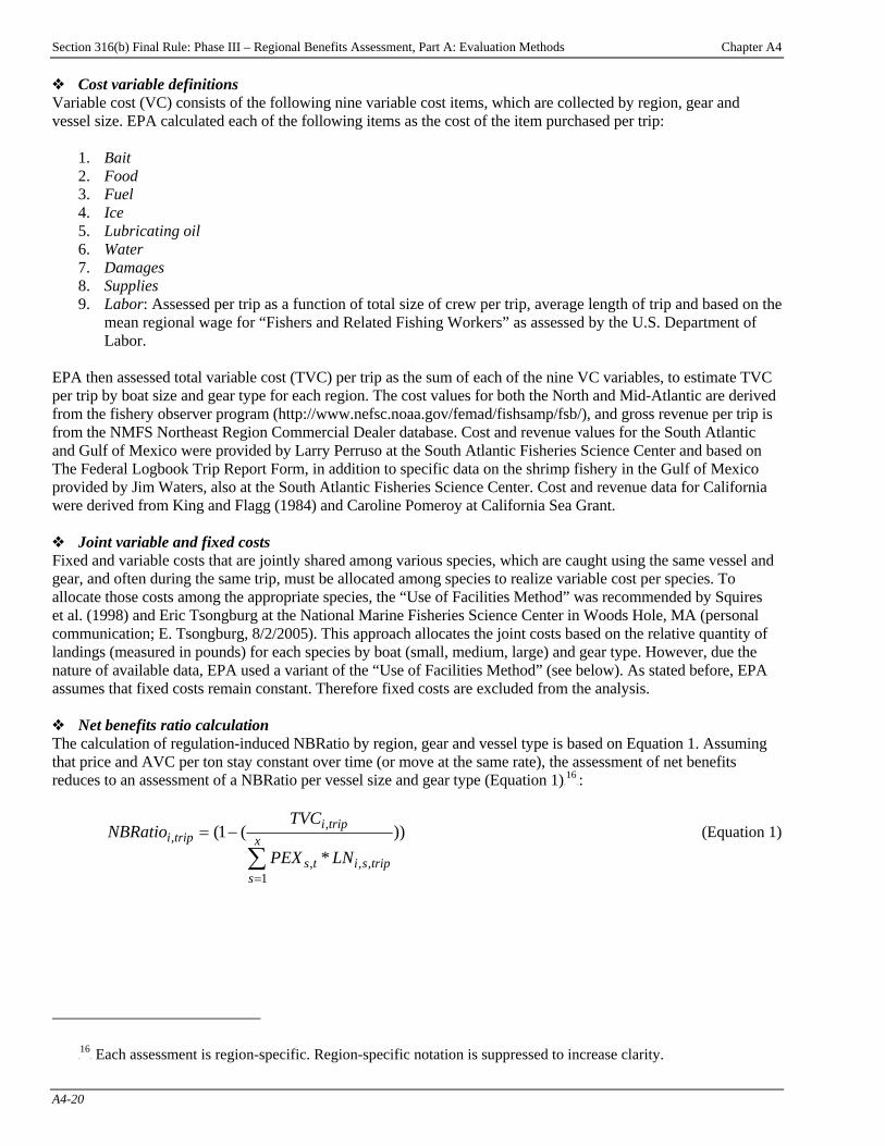
Section 316(b) Final Rule: Phase III – Regional Benefits Assessment, Part A: Evaluation Methods Chapter A4
A4-20
˜ Cost variable definitions Variable cost (VC) consists of the following nine variable cost items, which are collected by region, gear and vessel size. EPA calculated each of the following items as the cost of the item purchased per trip:
1. Bait 2. Food 3. Fuel 4. Ice 5. Lubricating oil 6. Water 7. Damages 8. Supplies 9. Labor: Assessed per trip as a function of total size of crew per trip, average length of trip and based on the
mean regional wage for “Fishers and Related Fishing Workers” as assessed by the U.S. Department of Labor.
EPA then assessed total variable cost (TVC) per trip as the sum of each of the nine VC variables, to estimate TVC per trip by boat size and gear type for each region. The cost values for both the North and Mid-Atlantic are derived from the fishery observer program (http://www.nefsc.noaa.gov/femad/fishsamp/fsb/), and gross revenue per trip is from the NMFS Northeast Region Commercial Dealer database. Cost and revenue values for the South Atlantic and Gulf of Mexico were provided by Larry Perruso at the South Atlantic Fisheries Science Center and based on The Federal Logbook Trip Report Form, in addition to specific data on the shrimp fishery in the Gulf of Mexico provided by Jim Waters, also at the South Atlantic Fisheries Science Center. Cost and revenue data for California were derived from King and Flagg (1984) and Caroline Pomeroy at California Sea Grant. ˜ Joint variable and fixed costs Fixed and variable costs that are jointly shared among various species, which are caught using the same vessel and gear, and often during the same trip, must be allocated among species to realize variable cost per species. To allocate those costs among the appropriate species, the “Use of Facilities Method” was recommended by Squires et al. (1998) and Eric Tsongburg at the National Marine Fisheries Science Center in Woods Hole, MA (personal communication; E. Tsongburg, 8/2/2005). This approach allocates the joint costs based on the relative quantity of landings (measured in pounds) for each species by boat (small, medium, large) and gear type. However, due the nature of available data, EPA used a variant of the “Use of Facilities Method” (see below). As stated before, EPA assumes that fixed costs remain constant. Therefore fixed costs are excluded from the analysis. ˜ Net benefits ratio calculation The calculation of regulation-induced NBRatio by region, gear and vessel type is based on Equation 1. Assuming that price and AVC per ton stay constant over time (or move at the same rate), the assessment of net benefits reduces to an assessment of a NBRatio per vessel size and gear type (Equation 1)TPF
16FPT:
))*
(1(
1,,,
,,
∑=
−= x
stripsits
tripitripi
LNPEX
TVCNBRatio (Equation 1)
TP
16PT Each assessment is region-specific. Region-specific notation is suppressed to increase clarity.
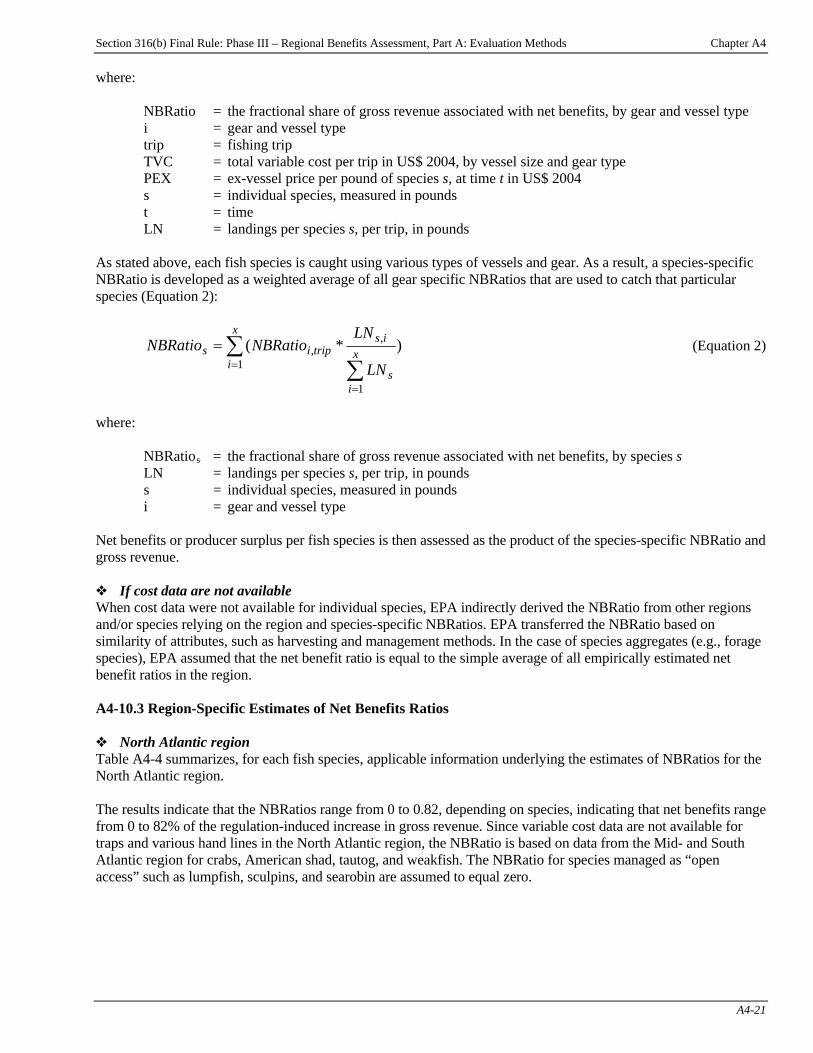
Section 316(b) Final Rule: Phase III – Regional Benefits Assessment, Part A: Evaluation Methods Chapter A4
A4-21
where:
NBRatio = the fractional share of gross revenue associated with net benefits, by gear and vessel type i = gear and vessel type trip = fishing trip TVC = total variable cost per trip in US$ 2004, by vessel size and gear type PEX = ex-vessel price per pound of species s, at time t in US$ 2004 s = individual species, measured in pounds t = time LN = landings per species s, per trip, in pounds
As stated above, each fish species is caught using various types of vessels and gear. As a result, a species-specific NBRatio is developed as a weighted average of all gear specific NBRatios that are used to catch that particular species (Equation 2):
)*(1
1
,,∑
∑=
=
=x
ix
is
istripis
LN
LNNBRatioNBRatio (Equation 2)
where:
NBRatioBsB = the fractional share of gross revenue associated with net benefits, by species s LN = landings per species s, per trip, in pounds s = individual species, measured in pounds i = gear and vessel type
Net benefits or producer surplus per fish species is then assessed as the product of the species-specific NBRatio and gross revenue. ˜ If cost data are not available When cost data were not available for individual species, EPA indirectly derived the NBRatio from other regions and/or species relying on the region and species-specific NBRatios. EPA transferred the NBRatio based on similarity of attributes, such as harvesting and management methods. In the case of species aggregates (e.g., forage species), EPA assumed that the net benefit ratio is equal to the simple average of all empirically estimated net benefit ratios in the region. A4-10.3 Region-Specific Estimates of Net Benefits Ratios ˜ North Atlantic region Table A4-4 summarizes, for each fish species, applicable information underlying the estimates of NBRatios for the North Atlantic region. The results indicate that the NBRatios range from 0 to 0.82, depending on species, indicating that net benefits range from 0 to 82% of the regulation-induced increase in gross revenue. Since variable cost data are not available for traps and various hand lines in the North Atlantic region, the NBRatio is based on data from the Mid- and South Atlantic region for crabs, American shad, tautog, and weakfish. The NBRatio for species managed as “open access” such as lumpfish, sculpins, and searobin are assumed to equal zero.
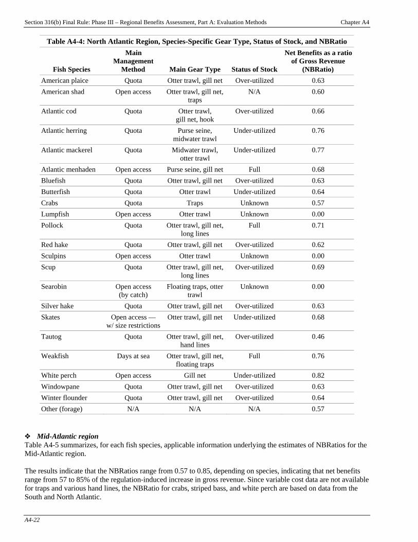
Section 316(b) Final Rule: Phase III – Regional Benefits Assessment, Part A: Evaluation Methods Chapter A4
A4-22
Table A4-4: North Atlantic Region, Species-Specific Gear Type, Status of Stock, and NBRatio
TFish SpeciesT
TMain Management
MethodT TMain Gear TypeT TStatus of StockT
TNet Benefits as a ratio of Gross Revenue
(NBRatio)T
American plaice Quota Otter trawl, gill net Over-utilized 0.63 American shad Open access Otter trawl, gill net,
traps N/A 0.60
Atlantic cod Quota Otter trawl, gill net, hook
Over-utilized 0.66
Atlantic herring Quota Purse seine, midwater trawl
Under-utilized 0.76
Atlantic mackerel Quota Midwater trawl, otter trawl
Under-utilized 0.77
Atlantic menhaden Open access Purse seine, gill net Full 0.68 Bluefish Quota Otter trawl, gill net Over-utilized 0.63 Butterfish Quota Otter trawl Under-utilized 0.64 Crabs Quota Traps Unknown 0.57 Lumpfish Open access Otter trawl Unknown 0.00 Pollock Quota Otter trawl, gill net,
long lines Full 0.71
Red hake Quota Otter trawl, gill net Over-utilized 0.62 Sculpins Open access Otter trawl Unknown 0.00 Scup Quota Otter trawl, gill net,
long lines Over-utilized 0.69
Searobin Open access (by catch)
Floating traps, otter trawl
Unknown 0.00
Silver hake Quota Otter trawl, gill net Over-utilized 0.63 Skates Open access —
w/ size restrictions Otter trawl, gill net Under-utilized 0.68
Tautog Quota Otter trawl, gill net, hand lines
Over-utilized 0.46
Weakfish Days at sea Otter trawl, gill net, floating traps
Full 0.76
White perch Open access Gill net Under-utilized 0.82 Windowpane Quota Otter trawl, gill net Over-utilized 0.63 Winter flounder Quota Otter trawl, gill net Over-utilized 0.64 Other (forage) N/A N/A N/A 0.57
˜ Mid-Atlantic region Table A4-5 summarizes, for each fish species, applicable information underlying the estimates of NBRatios for the Mid-Atlantic region. The results indicate that the NBRatios range from 0.57 to 0.85, depending on species, indicating that net benefits range from 57 to 85% of the regulation-induced increase in gross revenue. Since variable cost data are not available for traps and various hand lines, the NBRatio for crabs, striped bass, and white perch are based on data from the South and North Atlantic.

Section 316(b) Final Rule: Phase III – Regional Benefits Assessment, Part A: Evaluation Methods Chapter A4
A4-23
In the Mid-Atlantic region, none of the affected species is considered to be managed as purely “open access” since all have a defined management body and, as a result, could be converted to a different management regime.
Table A4-5: Mid-Atlantic Region, Species-Specific Gear Type, Status of Stock, and NBRatio
TFish SpeciesT
TMain Management
MethodT TMain Gear TypeT
TStatus of StockT
TNet Benefits as a % of Gross Revenue
(NBRatio)T
Alewife Open access (by catch)
Gill net Over-utilized 0.85
American shad Open access Gill net Over-utilized 0.84 Atlantic croaker Open access
(by catch) Otter trawl,
gill net Over-utilized 0.74
Atlantic menhaden Open access Purse seine, otter trawl, gill net
N/A 0.67
Blue crab Size Traps Unknown 0.57 Other (commercial) N/A N/A N/A 0.73 Other (commercial and recreation)
N/A N/A N/A 0.73
Spot Open access (by catch)
Gill net Unknown 0.84
Striped bass Quota Gill net, otter trawl, hand lines
Full 0.67
Summer flounder Quota Otter trawl, long lines, gill net
Over-utilized 0.65
Weakfish Per trip quota Otter trawl, long lines, gill net
Full 0.76
White perch Open access Otter trawl, long lines, gill net, purse seines
Under-utilized 0.82
Windowpane Quota Otter trawl, gill net Over-utilized 0.70 Winter flounder Quota Otter trawl, gill net Over-utilized 0.70 Other (forage) N/A N/A N/A 0.73
˜ South Atlantic region Table A4-6 summarizes, for each fish species, applicable information underlying the estimates of NBRatios for the South Atlantic region. The results indicate that the NBRatios range from 0.39 to 0.76, depending on species, indicating that net benefits range from 39 to 76% of the regulation-induced increase in gross revenue. In the South Atlantic region, none of the affected species is considered to be managed as purely “open access” since all have a defined management body and, as a result, could be converted to a different management regime.
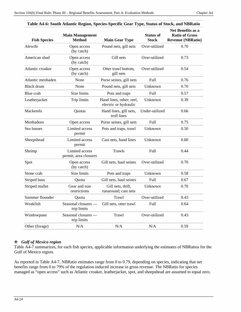
Section 316(b) Final Rule: Phase III – Regional Benefits Assessment, Part A: Evaluation Methods Chapter A4
A4-24
Table A4-6: South Atlantic Region, Species-Specific Gear Type, Status of Stock, and NBRatio
TFish SpeciesT
TMain Management MethodT TMain Gear TypeT
TStatus of StockT
TNet Benefits as a Ratio of Gross
Revenue (NBRatio)T
Alewife Open access (by catch)
Pound nets, gill nets Over-utilized 0.70
American shad Open access (by catch)
Gill nets Over-utilized 0.73
Atlantic croaker Open access (by catch)
Otter trawl bottom, gill nets
Over-utilized 0.54
Atlantic menhaden None Purse seines, gill nets Full 0.76 Black drum None Pound nets, gill nets Unknown 0.70
Blue crab Size limits Pots and traps Full 0.57 Leatherjacket Trip limits Hand lines, other; reel,
electric or hydraulic Unknown 0.39
Mackerels Quotas Hand lines, gill nets, troll lines
Under-utilized 0.66
Menhadens Open access Purse seines, gill nets Full 0.75 Sea basses Limited access
permit Pots and traps, trawl Unknown 0.50
Sheepshead Limited access permit
Cast nets, hand lines Unknown 0.60
Shrimp Limited access permit, area closures
Trawls Full 0.44
Spot Open access (by catch)
Gill nets, haul seines Over-utilized 0.70
Stone crab Size limits Pots and traps Unknown 0.58 Striped bass Quota Gill nets, haul seines Full 0.67 Striped mullet Gear and size
restrictions Gill nets, drift,
runaround; cast nets Unknown 0.70
Summer flounder Quota Trawl Over-utilized 0.43 Weakfish Seasonal closures —
trip limits Gill nets, otter trawl Full 0.64
Windowpane Seasonal closures — trip limits
Trawl Over-utilized 0.43
Other (forage) N/A N/A N/A 0.59 ˜ Gulf of Mexico region Table A4-7 summarizes, for each fish species, applicable information underlying the estimates of NBRatios for the Gulf of Mexico region. As reported in Table A4-7, NBRatio estimates range from 0 to 0.79, depending on species, indicating that net benefits range from 0 to 79% of the regulation-induced increase in gross revenue. The NBRatio for species managed as “open access” such as Atlantic croaker, leatherjacket, spot, and sheepshead are assumed to equal zero.
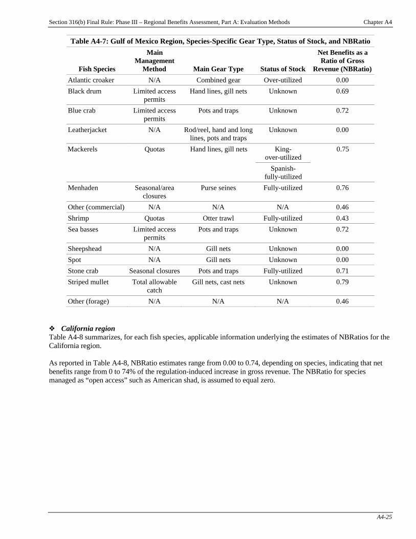
Section 316(b) Final Rule: Phase III – Regional Benefits Assessment, Part A: Evaluation Methods Chapter A4
A4-25
Table A4-7: Gulf of Mexico Region, Species-Specific Gear Type, Status of Stock, and NBRatio
TFish SpeciesT
TMain Management
MethodT TMain Gear TypeT TStatus of StockT
TNet Benefits as a Ratio of Gross
Revenue (NBRatio)T
Atlantic croaker N/A Combined gear Over-utilized 0.00 Black drum Limited access
permits Hand lines, gill nets Unknown 0.69
Blue crab Limited access permits
Pots and traps Unknown 0.72
Leatherjacket N/A Rod/reel, hand and long lines, pots and traps
Unknown 0.00
Mackerels King- over-utilized
Quotas Hand lines, gill nets
Spanish- fully-utilized
0.75
Menhaden Seasonal/area closures
Purse seines Fully-utilized 0.76
Other (commercial) N/A N/A N/A 0.46 Shrimp Quotas Otter trawl Fully-utilized 0.43 Sea basses Limited access
permits Pots and traps Unknown 0.72
Sheepshead N/A Gill nets Unknown 0.00 Spot N/A Gill nets Unknown 0.00 Stone crab Seasonal closures Pots and traps Fully-utilized 0.71 Striped mullet Total allowable
catch Gill nets, cast nets Unknown 0.79
Other (forage) N/A N/A N/A 0.46 ˜ California region Table A4-8 summarizes, for each fish species, applicable information underlying the estimates of NBRatios for the California region. As reported in Table A4-8, NBRatio estimates range from 0.00 to 0.74, depending on species, indicating that net benefits range from 0 to 74% of the regulation-induced increase in gross revenue. The NBRatio for species managed as “open access” such as American shad, is assumed to equal zero.
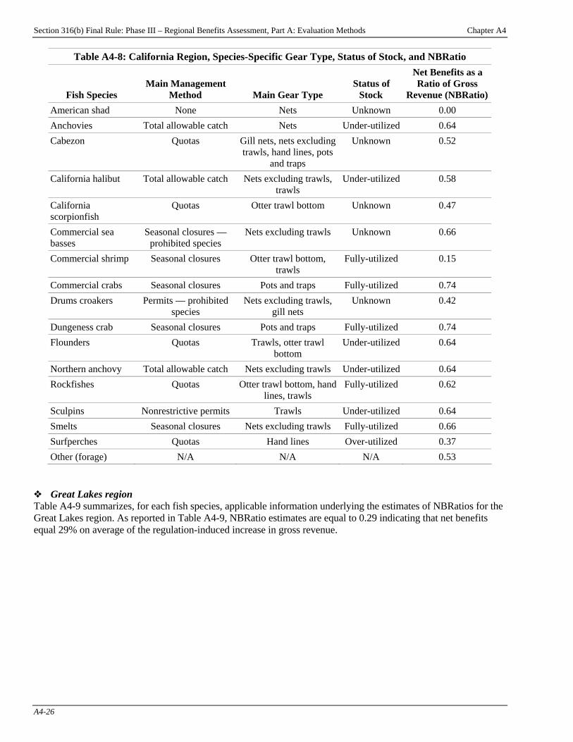
Section 316(b) Final Rule: Phase III – Regional Benefits Assessment, Part A: Evaluation Methods Chapter A4
A4-26
Table A4-8: California Region, Species-Specific Gear Type, Status of Stock, and NBRatio
TFish SpeciesT
TMain Management MethodT TMain Gear TypeT
TStatus of StockT
TNet Benefits as a Ratio of Gross
Revenue (NBRatio)T
American shad None Nets Unknown 0.00 Anchovies Total allowable catch Nets Under-utilized 0.64 Cabezon Quotas Gill nets, nets excluding
trawls, hand lines, pots and traps
Unknown 0.52
California halibut Total allowable catch Nets excluding trawls, trawls
Under-utilized 0.58
California scorpionfish
Quotas Otter trawl bottom Unknown 0.47
Commercial sea basses
Seasonal closures — prohibited species
Nets excluding trawls Unknown 0.66
Commercial shrimp Seasonal closures Otter trawl bottom, trawls
Fully-utilized 0.15
Commercial crabs Seasonal closures Pots and traps Fully-utilized 0.74 Drums croakers Permits — prohibited
species Nets excluding trawls,
gill nets Unknown 0.42
Dungeness crab Seasonal closures Pots and traps Fully-utilized 0.74 Flounders Quotas Trawls, otter trawl
bottom Under-utilized 0.64
Northern anchovy Total allowable catch Nets excluding trawls Under-utilized 0.64 Rockfishes Quotas Otter trawl bottom, hand
lines, trawls Fully-utilized 0.62
Sculpins Nonrestrictive permits Trawls Under-utilized 0.64 Smelts Seasonal closures Nets excluding trawls Fully-utilized 0.66 Surfperches Quotas Hand lines Over-utilized 0.37 Other (forage) N/A N/A N/A 0.53
˜ Great Lakes region Table A4-9 summarizes, for each fish species, applicable information underlying the estimates of NBRatios for the Great Lakes region. As reported in Table A4-9, NBRatio estimates are equal to 0.29 indicating that net benefits equal 29% on average of the regulation-induced increase in gross revenue.
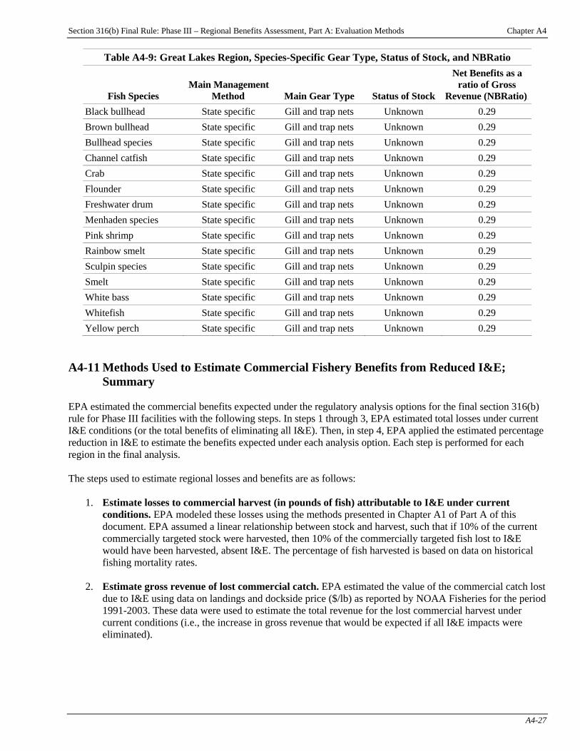
Section 316(b) Final Rule: Phase III – Regional Benefits Assessment, Part A: Evaluation Methods Chapter A4
A4-27
Table A4-9: Great Lakes Region, Species-Specific Gear Type, Status of Stock, and NBRatio
TFish SpeciesT
TMain Management MethodT TMain Gear TypeT TStatus of StockT
TNet Benefits as a ratio of Gross
Revenue (NBRatio)TTT
Black bullhead State specific Gill and trap nets Unknown 0.29 Brown bullhead State specific Gill and trap nets Unknown 0.29 Bullhead species State specific Gill and trap nets Unknown 0.29 Channel catfish State specific Gill and trap nets Unknown 0.29 Crab State specific Gill and trap nets Unknown 0.29 Flounder State specific Gill and trap nets Unknown 0.29 Freshwater drum State specific Gill and trap nets Unknown 0.29 Menhaden species State specific Gill and trap nets Unknown 0.29 Pink shrimp State specific Gill and trap nets Unknown 0.29 Rainbow smelt State specific Gill and trap nets Unknown 0.29 Sculpin species State specific Gill and trap nets Unknown 0.29 Smelt State specific Gill and trap nets Unknown 0.29 White bass State specific Gill and trap nets Unknown 0.29 Whitefish State specific Gill and trap nets Unknown 0.29 Yellow perch State specific Gill and trap nets Unknown 0.29
A4-11 Methods Used to Estimate Commercial Fishery Benefits from Reduced I&E;
Summary EPA estimated the commercial benefits expected under the regulatory analysis options for the final section 316(b) rule for Phase III facilities with the following steps. In steps 1 through 3, EPA estimated total losses under current I&E conditions (or the total benefits of eliminating all I&E). Then, in step 4, EPA applied the estimated percentage reduction in I&E to estimate the benefits expected under each analysis option. Each step is performed for each region in the final analysis. The steps used to estimate regional losses and benefits are as follows:
1. Estimate losses to commercial harvest (in pounds of fish) attributable to I&E under current conditions. EPA modeled these losses using the methods presented in Chapter A1 of Part A of this document. EPA assumed a linear relationship between stock and harvest, such that if 10% of the current commercially targeted stock were harvested, then 10% of the commercially targeted fish lost to I&E would have been harvested, absent I&E. The percentage of fish harvested is based on data on historical fishing mortality rates.
2. Estimate gross revenue of lost commercial catch. EPA estimated the value of the commercial catch lost
due to I&E using data on landings and dockside price ($/lb) as reported by NOAA Fisheries for the period 1991-2003. These data were used to estimate the total revenue for the lost commercial harvest under current conditions (i.e., the increase in gross revenue that would be expected if all I&E impacts were eliminated).

Section 316(b) Final Rule: Phase III – Regional Benefits Assessment, Part A: Evaluation Methods Chapter A4
A4-28
3. Estimate lost economic surplus. The conceptually appropriate measure of benefits is the sum of any changes in producer and consumer surplus. The methods used for estimating the change in surplus depend on whether the physical impact on the commercial fishery market appears sufficiently small such that it is reasonable to assume there will be no appreciable price changes in the markets for the impacted fisheries.
a. For the regions included in this analysis, it is reasonable to assume no change in price, which implies that the welfare change is limited to changes in producer surplus. This change in producer surplus, captured by “normal profits,” is assumed to be equivalent to a fixed proportion of the change in gross revenues, as developed under step 2. EPA estimated species- and region-specific ratios (NBRatios) between producer surplus and gross revenue, as presented in section A4-10. EPA then applied the NBRatio to the estimated lost revenue to estimate total lost economic surplus. This ratio ranges from 0 to 84%.
b. EPA believes this is an appropriate approach to estimating producer surplus when there are no anticipated price changes. EPA’s Guidelines for Preparing Economic Analyses (U.S. EPA, 2000a; EPA 240-R-00-003) describes options for estimating ecological benefits for fisheries, and note that “if changes in service flows are small, current market prices can be used as a proxy for expected benefit . . . a change in the commercial fish catch might be valued using the market price for the affected species.” This statement indicates that 100% of the gross revenue change, based on current prices, may be a suitable measure of value and this analysis takes a similar approach.
4. Estimate increase in surplus attributable to the regulatory analysis options. Once the commercial
surplus losses associated with I&E under baseline conditions were estimated according to the approaches outlined in steps 2 and 3, EPA estimated the percentage reduction in I&E at each facility under each regulatory analysis option. This analysis was conducted for each region. EPA computed the increase in gross revenue using the method described in step 2, and then estimated the producer surplus using the fractional approach described in step 3.
A4-12 Limitations and Uncertainties Table A4-10 summarizes the caveats, omissions, biases and uncertainties known to affect the estimates that were developed for the benefits analysis.

Section 316(b) Final Rule: Phase III – Regional Benefits Assessment, Part A: Evaluation Methods Chapter A4
A4-29
Table A4-10: Caveats, Omissions, Biases, and Uncertainties in the Commercial Benefits Estimates Issue Impact on Benefits Estimate Comments
Change in commercial landings due to I&E is uncertain
Uncertain Projected changes in harvest may be under-estimated because neither cumulative impacts of I&E over time nor interactions with other stressors are considered.
Some estimates of commercial harvest losses due to I&E under current conditions are not region/species-specific
Uncertain EPA estimated the impact of I&E in the case study analyses based on data provided by the facilities. The most current data available were used. However, in some cases these data are 20 years old or older. Thus, they may not reflect current conditions.
TEffect of change in stocks on landings is not consideredT
Uncertain EPA assumed a linear stock to harvest relationship, so that a 10% change in stock would have a 10% change in landings; this may be low or high, depending on the condition of the stocks. Region-specific fisheries regulations also will affect the validity of the linear assumption.
TEffect of uncertainty in estimates of commercial landings and prices is unknownT
Uncertain EPA assumes that NOAA landings data are accurate and complete. In some cases prices and/or quantities may be reported incorrectly.
Section 316(b) Final Rule: Phase III – Regional Benefits Assessment, Part A: Evaluation Methods Chapter A5
A5-1
Chapter A5: Recreational Fishing Benefits Methodology
Introduction EPA used a benefit transfer approach to estimate the welfare gain to recreational anglers from improved recreational fishing opportunities due to reductions in impingement and entrainment (I&E) under the regulatory analysis options considered for the final section 316(b) rule for Phase III existing facilities. Benefit transfer involves adapting research conducted for another purpose to address the policy questions at hand (Bergstrom and De Civita, 1999). Although primary research methods are generally preferred to benefit transfer methods, benefit transfer is often the second (or only) alternative to original studies due to resource or data constraints. EPA notes that Smith et al. (2002, p. 134) state that “. . . nearly all benefit cost analyses rely on benefit transfers . . ..” For the Phase III analysis, EPA used a benefit transfer approach based on a meta-analysis to evaluate recreational fishing benefits of the regulatory analysis options for all study regions. To validate the meta-analysis results, EPA also used regional random utility models (RUM) of recreational fishing behavior developed for the Phase II analysis to estimate welfare gain to recreational anglers from improved recreational opportunities resulting from reduced I&E of fish species at Phase III facilities. EPA used the RUM approach to validate results for the four coastal regions and the Great Lakes region, but was unavailable for the Inland region because of a lack of data on Inland site characteristics, including baseline catch rates and presence of boat ramps and other recreational amenities. Chapter A11 of the Phase II Regional Analysis document provides a more detailed discussion of the methodology used in EPA’s RUM analysis (U.S. EPA, 2004a).
Chapter Contents A5-1 Literature Review Procedure and Organization................................................. A5-2 A5-2 Description of Studies .................................. A5-3 A5-3 Meta-Analysis of Recreational Fishing Studies: Regression Model......................... A5-10 A5-3.1 Meta-Data ..................................... A5-10 A5-3.2 Model and Results ........................ A5-17 A5-3.3 Interpretation of Regression Analysis Results ........................... A5-20 A5-4 Application of the Meta-Analysis Results
to the Analysis of Recreational Benefits of the Section 316(b) Regulatory Analysis Options for Phase III Facilities................... A5-23
A5-4.1 Estimating Marginal Value per Fish ............................................... A5-23 A5-4.2 Calculating Recreational Benefits......................................... A5-26 A5-5 Limitations and Uncertainties .................... A5-26 A5-5.1 Sensitivity Analysis Based on Krinsky and Robb (1986) Approach ...................................... A5-27 A5-5.2 Variable Assignments for Independent Regressors ................ A5-28 A5-5.3 Other Limitations and
Uncertainties................................. A5-28
Benefit transfer methods fall within three fundamental classes: (1) transfer of an unadjusted fixed value estimate generated from a single study site, (2) the use of expert judgment to aggregate or otherwise alter benefits to be transferred from a site or set of sites, and (3) estimation of a value estimator model derived from study site data, often from multiple sites (Bergstrom and De Civita, 1999). Recent studies have shown little support for the accuracy or validity of the first method, leading to increased attention to, and use of, adjusted values estimated by one of the remaining two approaches (Bergstrom and De Civita, 1999).
Section 316(b) Final Rule: Phase III – Regional Benefits Assessment, Part A: Evaluation Methods Chapter A5
A5-2
The third class of benefit transfer approaches includes meta-analysis techniques, which have been increasingly explored by economists as a potential basis of policy analysis conducted by various government agencies charged with the stewardship of natural resources.TPF
1FPT Although there are few generally accepted guidelines for meta-
analyses applied to environmental policy, EPA believes that this is a promising methodology for policy evaluation. This chapter describes how EPA applied meta-analysis, which is often cited as a more appropriate means of benefit transfer, to estimate the welfare gain associated with improved recreational catch. The first step in implementing an “adjusted value” benefit transfer approach is a systematic analysis of the available economic studies that estimate the welfare gain associated with improved recreational catch. The Agency identified 48 valuation studies that use stated preference or revealed preference techniques to elicit benefit values for changes in recreational catch. All of these studies provide estimates of the marginal value to fishers of catching an additional fish, or provide sufficient information for EPA to calculate such a value. These studies vary in several respects, including valuation methodology, survey administration method, species targeted by anglers, baseline catch rate, location, and economic and demographic characteristics of the sample. To examine the relative influence of study, economic, and resource characteristics on willingness-to-pay (WTP) for catching an additional fish, the Agency conducted a regression-based meta-analyses of 391 estimates of WTP (or marginal value) per fish, provided by the 48 original studies. The estimated econometric model can be used to calculate per fish values for species that are potentially affected by I&E. The following discussion summarizes the results of EPA’s analysis of recreational fishing studies and outlines the methodology for applying meta-regression results to the estimation of benefits from reduced I&E attributable to the regulatory analysis options. A5-1 Literature Review Procedure and Organization EPA performed an in-depth search of the economic literature to identify valuation studies that estimate — or provide sufficient information to calculate — the value that anglers place on catching an additional fish. EPA used a variety of sources and search methods to identify relevant studies:
< review of EPA’s research and bibliographies dealing with the recreational benefits of fishing; < systematic review of recent issues of resource economics journals (e.g., Land Economics, Journal of
Agricultural and Resource Economics, Journal of Environmental Economics and Management, Water Resources Research);
< searches of online reference and abstract databases [e.g., Environmental Valuation Resource Inventory (EVRI), the Fish and Wildlife Service’s Database of Sportfishing Values];
< queries to academic search engines (e.g., EconLit, ISI Web of Science, Index of Digital Dissertations); < visits to homepages of authors known to have published valuation studies of recreational fishing; < searches of web sites of agricultural and resource economics departments at several colleges and
universities; and < searches of web sites of organizations and agencies known to publish environmental and resource
economics valuation research [e.g., Resources for the Future (RFF), National Center for Environmental Economics (NCEE), National Oceanic and Atmospheric Administration (NOAA), Library of Congress’ Congressional Research Service].
TP
1PT Meta-analysis is “the statistical analysis of a large collection of results for individual studies for the purposes of
integrating the findings” (Glass, 1976).
Section 316(b) Final Rule: Phase III – Regional Benefits Assessment, Part A: Evaluation Methods Chapter A5
A5-3
From this review, EPA identified approximately 450 journal articles, academic working papers, reports, books, and dissertations that were potentially relevant for this analysis. Forty-eight of these studies were included in the data set for the recreational meta-analysis because they met the criteria listed below:
< Specific amenity valued: Selected studies were limited to those that estimated WTP that recreational anglers place on catching an additional fish or provided sufficient information for EPA to calculate such a value;
< Location: Selected studies were limited to those that surveyed U.S. or Canadian populations; and < Research methods: Selected studies were limited to those that applied primary research methods
supported by journal literature.
The Agency utilized information from each of the studies to compile an extensive data set for use in the meta-analysis. The complete data set is provided in the public record for the proposed rule (see DCN 7-4923 and DCN 7-4924), and includes the following information:
< full study citation; < study methodology (e.g., research method, survey administration method, question format); < sample characteristics (e.g., sample size, response rate, income, age, gender); < study location (e.g., waterbody name, waterbody type, geographic location); < description of fishing quality (e.g., target species, fishing mode, baseline catch rate, post-change catch
rate); < marginal value per fish, updated to 2004 dollars; and < methods for obtaining marginal values per fish (i.e., whether marginal value per fish was directly
available from the study, marginal value calculation method). A5-2 Description of Studies As noted above, EPA selected 48 recreational angling valuation studies that allow estimation of the value of catching an additional fish. These studies were published between 1982 and 2004, and are based on data from surveys conducted between 1977 and 2001. The studies all apply standard, generally accepted valuation methods, such as contingent valuation, travel cost models, and random utility models, to assess marginal value per fish. Studies were excluded if they did not conform to general concepts of economic theory, or if they applied methods not generally accepted in the economic literature. All selected studies focus on changes in recreational catch rates in the U.S. or Canada. Beyond this general similarity, the studies vary in several respects. Differences include the species targeted by anglers, the magnitude of the change in catch rates, the location of the study, the survey administration method, demographics of the survey sample, and statistical methods employed. The 48 studies include 24 journal articles, 15 reports, five Ph.D. dissertations, three academic or staff papers, and one book. Twenty studies share a primary author with at least one other study. These 20 studies have a combined total of eight individuals as primary authors. Because multiple estimates of the marginal per-fish value are available from most of the studies, the 48 studies selected for the meta-analysis provide 391 observations for the final data set. Some of the characteristics that allow multiple observations to be derived from a single study include variations in the baseline catch rate, the species being valued, the locations where fish were caught, the fishing method (i.e., boat or shore), and the valuation methodology.

Section 316(b) Final Rule: Phase III – Regional Benefits Assessment, Part A: Evaluation Methods Chapter A5
A5-4
Survey response rates from the studies range from 38% to 99%, and study sample sizes range from 72 to 36,802 responses. Two hundred and ten estimates from 21 studies are based on random utility models, 59 estimates from 11 studies are based on travel cost models, and 122 estimates from 20 studies are based on stated preference methods.TPF
2FPT EPA calculated the marginal value per fish based on information provided in the study for 93 estimates
from 15 studies, and for the remaining estimates the marginal values were provided by the authors. Table A5-1 lists key study and resource characteristics and indicates the number of observations derived from each study. From these 48 studies, the Agency compiled a data set for the meta-analysis of marginal values per fish. The following section describes the estimation of this model and its application to the regulatory analysis options for Phase III facilities.
TP
2PT The number of studies employing each valuation methodology does not sum to the total number of studies
because some studies used different valuation methods, from which multiple observations were derived.
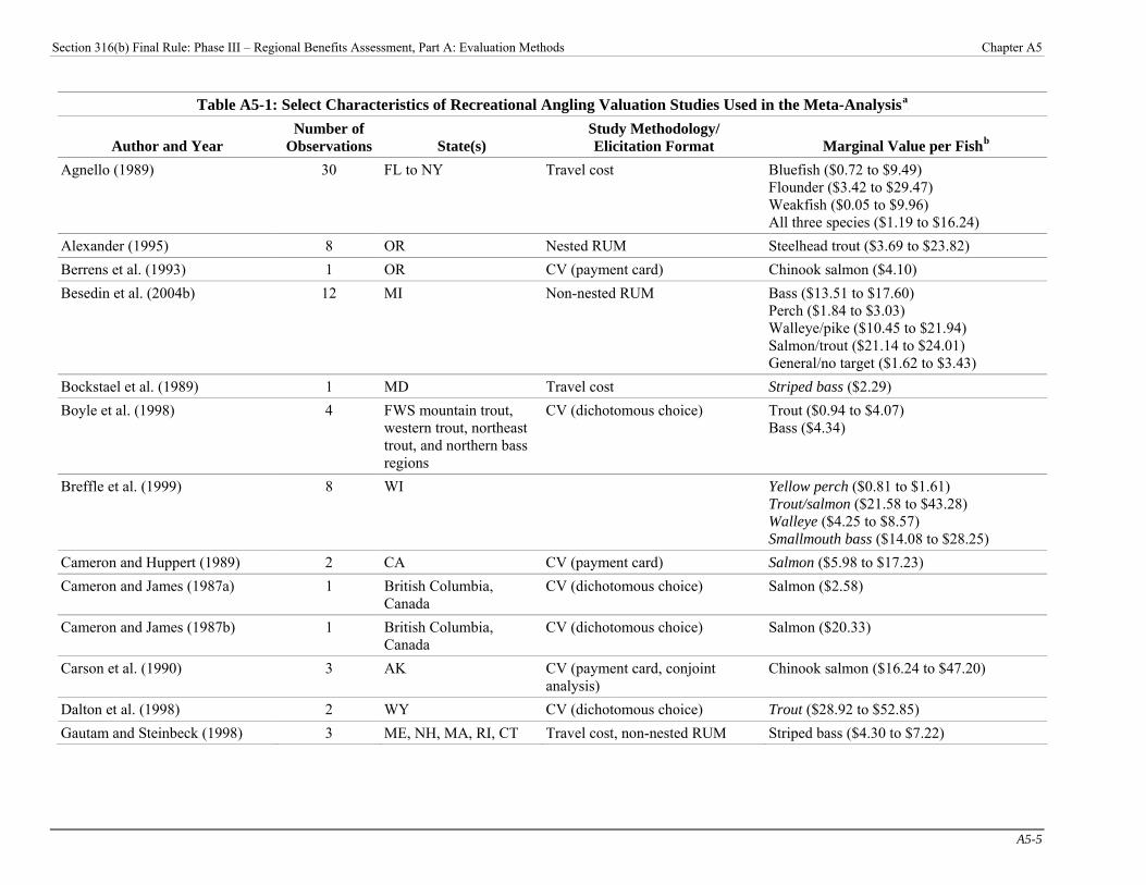
Section 316(b) Final Rule: Phase III – Regional Benefits Assessment, Part A: Evaluation Methods Chapter A5
A5-5
Table A5-1: Select Characteristics of Recreational Angling Valuation Studies Used in the Meta-AnalysisP
aP
Author and Year Number of
Observations State(s) Study Methodology/ Elicitation Format Marginal Value per FishP
bP
Agnello (1989) 30 FL to NY Travel cost Bluefish ($0.72 to $9.49) Flounder ($3.42 to $29.47) Weakfish ($0.05 to $9.96) All three species ($1.19 to $16.24)
Alexander (1995) 8 OR Nested RUM Steelhead trout ($3.69 to $23.82) Berrens et al. (1993) 1 OR CV (payment card) Chinook salmon ($4.10) Besedin et al. (2004b) 12 MI Non-nested RUM Bass ($13.51 to $17.60)
Perch ($1.84 to $3.03) Walleye/pike ($10.45 to $21.94) Salmon/trout ($21.14 to $24.01) General/no target ($1.62 to $3.43)
Bockstael et al. (1989) 1 MD Travel cost Striped bass ($2.29) Boyle et al. (1998) 4 FWS mountain trout,
western trout, northeast trout, and northern bass regions
CV (dichotomous choice) Trout ($0.94 to $4.07) Bass ($4.34)
Breffle et al. (1999) 8 WI Yellow perch ($0.81 to $1.61) Trout/salmon ($21.58 to $43.28) Walleye ($4.25 to $8.57) Smallmouth bass ($14.08 to $28.25)
Cameron and Huppert (1989) 2 CA CV (payment card) Salmon ($5.98 to $17.23) Cameron and James (1987a) 1 British Columbia,
Canada CV (dichotomous choice) Salmon ($2.58)
Cameron and James (1987b) 1 British Columbia, Canada
CV (dichotomous choice) Salmon ($20.33)
Carson et al. (1990) 3 AK CV (payment card, conjoint analysis)
Chinook salmon ($16.24 to $47.20)
Dalton et al. (1998) 2 WY CV (dichotomous choice) Trout ($28.92 to $52.85) Gautam and Steinbeck (1998) 3 ME, NH, MA, RI, CT Travel cost, non-nested RUM Striped bass ($4.30 to $7.22)

Section 316(b) Final Rule: Phase III – Regional Benefits Assessment, Part A: Evaluation Methods Chapter A5
A5-6
Table A5-1: Select Characteristics of Recreational Angling Valuation Studies Used in the Meta-AnalysisP
aP
Author and Year Number of
Observations State(s) Study Methodology/ Elicitation Format Marginal Value per FishP
bP
Hicks et al. (1999) 44 ME, NH, MA, RI, CT, NY, NJ, DE, MD, VA
Nested RUM Big game ($5.83 to $8.42) Bottomfish ($2.08 to $3.34) Small game ($3.09 to $4.77) Flatfish ($3.95 to $7.33)
Hicks (2002) 3 NH to VA CV (conjoint analysis), non-nested RUM
Summer flounder ($2.66 to $4.78)
Huppert (1989) 3 CA CV (payment card), travel cost Chinook salmon and striped bass ($7.96 to $60.08)
Hushak et al. (1988) 3 OH Travel cost Walleye ($2.41 to $3.22) Johnson et al. (1995) 19 CO CV (iterative bidding,
dichotomous choice) Trout ($0.56 to $3.02)
Johnson (1989) 5 CO CV (iterative bidding) Brown and rainbow trout ($0.89 to $1.66) Rainbow trout ($2.65)
Johnson and Adams (1989) 1 OR CV (multiple methods) Steelhead trout ($11.46) Jones and Stokes Associates (1987)
4 AK Non-nested RUM Halibut ($158.22) Chinook salmon ($336.45) Coho salmon ($183.65) Dolly varden ($23.90)
Kirkley et al. (1999) 10 VA CV (open-ended) Bottomfish and croaker ($3.14 to $13.24) Summer flounder ($4.82 to $20.47) Gamefish ($16.86 to $67.43) No target ($1.98 to $8.43)
Lee (1996) 5 WA CV (conjoint analysis) Trout ($1.16 to $3.94) Loomis (1988) 13 OR, WA Travel cost Steelhead trout ($42.11 to $187.33)
Salmon ($13.60 to $117.41) Lupi and Hoehn (1998) 3 MI Nested RUM Lake trout ($10.40 to $14.29)
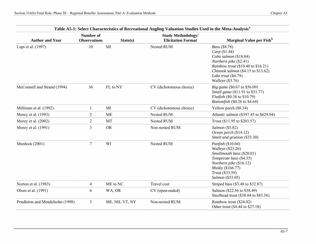
Section 316(b) Final Rule: Phase III – Regional Benefits Assessment, Part A: Evaluation Methods Chapter A5
A5-7
Table A5-1: Select Characteristics of Recreational Angling Valuation Studies Used in the Meta-AnalysisP
aP
Author and Year Number of
Observations State(s) Study Methodology/ Elicitation Format Marginal Value per FishP
bP
Lupi et al. (1997) 10 MI Nested RUM Bass ($8.78) Carp ($1.44) Coho salmon ($18.84) Northern pike ($2.41) Rainbow trout ($10.40 to $16.21) Chinook salmon ($4.15 to $13.62) Lake trout ($6.79) Walleye ($3.76)
McConnell and Strand (1994) 36 FL to NY CV (dichotomous choice) Big game ($0.67 to $56.09) Small game ($11.91 to $31.77) Flatfish ($0.38 to $10.79) Bottomfish ($0.26 to $4.64)
Milliman et al. (1992) 1 MI CV (dichotomous choice) Yellow perch ($0.34) Morey et al. (1993) 2 ME Nested RUM Atlantic salmon ($397.45 to $629.94) Morey et al. (2002) 2 MT Nested RUM Trout ($11.95 to $203.57) Morey et al. (1991) 3 OR Non-nested RUM Salmon ($5.82)
Ocean perch ($14.12) Smelt and grunion ($33.30)
Murdock (2001) 7 WI Nested RUM Panfish ($10.04) Walleye ($23.26) Smallmouth bass ($20.01) Temperate bass ($4.35) Northern pike ($16.12) Musky ($166.77) Trout ($33.59) Salmon ($53.05)
Norton et al. (1983) 4 ME to NC Travel cost Striped bass ($3.48 to $32.87) Olsen et al. (1991) 6 WA, OR CV (open-ended) Salmon ($22.56 to $38.49)
Steelhead trout ($38.04 to $83.56) Pendleton and Mendelsohn (1998) 3 ME, NH, VT, NY Non-nested RUM Rainbow trout ($24.02)
Other trout ($4.44 to $27.18)
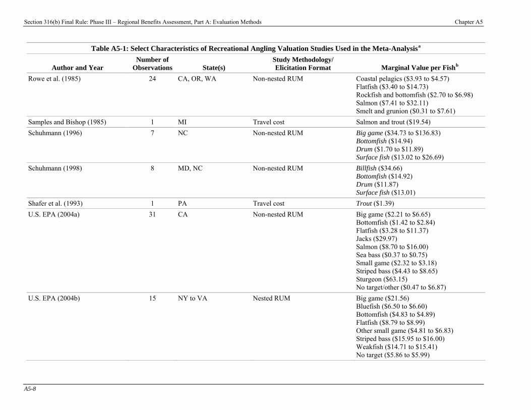
Section 316(b) Final Rule: Phase III – Regional Benefits Assessment, Part A: Evaluation Methods Chapter A5
A5-8
Table A5-1: Select Characteristics of Recreational Angling Valuation Studies Used in the Meta-AnalysisP
aP
Author and Year Number of
Observations State(s) Study Methodology/ Elicitation Format Marginal Value per FishP
bP
Rowe et al. (1985) 24 CA, OR, WA Non-nested RUM Coastal pelagics ($3.93 to $4.57) Flatfish ($3.40 to $14.73) Rockfish and bottomfish ($2.70 to $6.98) Salmon ($7.41 to $32.11) Smelt and grunion ($0.31 to $7.61)
Samples and Bishop (1985) 1 MI Travel cost Salmon and trout ($19.54) Schuhmann (1996) 7 NC Non-nested RUM Big game ($34.73 to $136.83)
Bottomfish ($14.94) Drum ($1.70 to $11.89) Surface fish ($13.02 to $26.69)
Schuhmann (1998) 8 MD, NC Non-nested RUM Billfish ($34.66) Bottomfish ($14.92) Drum ($11.87) Surface fish ($13.01)
Shafer et al. (1993) 1 PA Travel cost Trout ($1.39) U.S. EPA (2004a) 31 CA Non-nested RUM Big game ($2.21 to $6.65)
Bottomfish ($1.42 to $2.84) Flatfish ($3.28 to $11.37) Jacks ($29.97) Salmon ($8.70 to $16.00) Sea bass ($0.37 to $0.75) Small game ($2.32 to $3.18) Striped bass ($4.43 to $8.65) Sturgeon ($63.15) No target/other ($0.47 to $6.87)
U.S. EPA (2004b) 15 NY to VA Nested RUM Big game ($21.56) Bluefish ($6.50 to $6.60) Bottomfish ($4.83 to $4.89) Flatfish ($8.79 to $8.99) Other small game ($4.81 to $6.83) Striped bass ($15.95 to $16.00) Weakfish ($14.71 to $15.41) No target ($5.86 to $5.99)
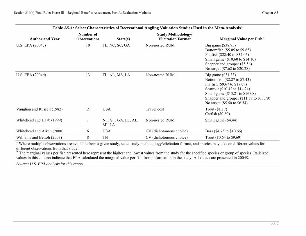
316(b) Final Rule: Phase III – Regional Benefits Assessment, Part A: Evaluation Methods Chapter A5
A5-9
U.S. EPA (2004c) 10 FL, NC, SC, GA Non-nested RUM Big game ($38.95) Bottomfish ($5.05 to $9.65) Flatfish ($28.40 to $32.05) Small game ($10.60 to $14.10) Snapper and grouper ($5.56) No target ($7.62 to $20.28)
U.S. EPA (2004d) 13 FL, AL, MS, LA Non-nested RUM Big game ($31.33) Bottomfish ($2.27 to $7.43) Flatfish ($9.67 to $17.09) Seatrout ($10.42 to $14.24) Small game ($13.21 to $16.08) Snapper and grouper ($11.59 to $11.79) No target ($5.50 to $6.54)
Vaughan and Russell (1982) 2 USA Travel cost Trout ($1.17) Catfish ($0.80)
Whitehead and Haab (1999) 1 NC, SC, GA, FL, AL, MI, LA
Non-nested RUM Small game ($4.44)
Whitehead and Aiken (2000) 6 USA CV (dichotomous choice) Bass ($4.73 to $10.66) Williams and Bettoli (2003) 8 TN CV (dichotomous choice) Trout ($0.64 to $9.69) P
aP Where multiple observations are available from a given study, state, study methodology/elicitation format, and species may take on different values for
different observations from that study. P
bP The marginal values per fish presented here represent the highest and lowest values from the study for the specified species or group of species. Italicized
values in this column indicate that EPA calculated the marginal value per fish from information in the study. All values are presented in 2004$. Source: U.S. EPA analysis for this report.
Table A5-1: Select Characteristics of Recreational Angling Valuation Studies Used in the Meta-AnalysisP
aP
Author and Year Number of
Observations State(s) Study Methodology/ Elicitation Format Marginal Value per FishP
bP
Section

Section 316(b) Final Rule: Phase III – Regional Benefits Assessment, Part A: Evaluation Methods Chapter A5
A5-10
A5-3 Meta-Analysis of Recreational Fishing Studies: Regression Model EPA estimated a meta-analysis model based on 391 estimates of the value anglers place on catching an additional fish, derived from 48 original studies. The meta-data, model specification, model results, and interpretation of those results are discussed in sections A5-3.1 through A5-3.3. In a frequently cited work, Glass (1976) characterizes meta-analysis as “the statistical analysis of a large collection of results for individual studies for the purposes of integrating the findings. It provides a rigorous alternative to the casual, narrative discussion of research studies which is commonly used to make some sense of the rapidly expanding research literature” [p. 3; cited in Poe et al. (2001), p. 138]. Meta-analysis is being increasingly explored as a potential means to estimate resource values in cases where original targeted research is impractical, or as a means to reveal systematic components of WTP (Smith and Osborne, 1996; Santos, 1998; Rosenberger and Loomis, 2000a; Poe et al., 2001; Woodward and Wui, 2001; Bateman and Jones, 2003; Johnston et al., 2003). While the literature urges caution in the use and interpretation of benefit transfers for direct policy application (e.g., Desvousges et al., 1998; Poe et al., 2001), such methods are “widely used in the United States by government agencies to facilitate benefit-cost analysis of public policies and projects affecting natural resources” (Bergstrom and De Civita, 1999). Transfers based on meta-analysis are common in both the United States and Canada (Bergstrom and De Civita, 1999). Depending on the suitability of available data, meta-analysis can provide a superior alternative to the calculation and use of a simple arithmetic mean WTP over the available observations, as it allows estimation of the systematic influence of study methodology, sample characteristics, and natural resource attributes on WTP (Johnston et al., 2003). The primary advantage of a regression-based (statistical) approach is that it accounts for differences among study characteristics that may contribute to changes in WTP, to the extent permitted by available data. An additional advantage is that meta-analysis can reveal systematic factors influencing WTP, allowing assessments of whether, for example, WTP estimates are (on average) sensitive to the baseline resource conditions (Smith and Osborne, 1996). A5-3.1 Meta-Data Meta-analysis is largely an empirical, data-driven process, but one in which variable and model selection is guided by theory. Given a reliance on information available from the underlying studies that comprise the meta-data, meta-analysis models most often represent a middle ground between model specifications that would be most theoretically appropriate and those specifications that are possible given available data. Smith and Osborne (1996), Rosenberger and Loomis (2000a), Poe et al. (2001), Bateman and Jones (2003), Dalhuisen et al. (2003), and others provide insight into the mechanics of specifying and estimating meta-equations in resource economics applications. To guide development of variable specifications, EPA relied upon a set of general principles. These principles are designed to prevent excessive data manipulations and other factors that may lead to misleading model results. The general principles include, all else being equal:
< models should attempt to capture elements of scale of resource changes; < models should focus on distinguishing marginal values associated with different types of species in
different regions, particularly where relevant to the policy question at hand; < in the absence of overriding theoretical considerations, continuous variables are generally preferred to
discrete variables derived from underlying continuous distributions; and < where possible, exogenous constraints should be avoided in favor of “letting the data speak for
themselves.” Based on these criteria, EPA selected a set of variables believed to have a potential influence on the estimated WTP per additional fish caught. Variable selection was guided primarily by prior findings in the literature, and constrained by information available from the original studies that comprise the meta-data. The dependent

Section 316(b) Final Rule: Phase III – Regional Benefits Assessment, Part A: Evaluation Methods Chapter A5
A5-11
variable chosen for the meta-analysis is the natural logarithm of WTP per fish, as reported in each original study or as calculated by EPA from information provided by the studies. EPA chose to use the natural log of the dependent variable instead of the linear form, based on (1) data fit, (2) the intuitive nature of results, and (3) the common use of this functional form in the meta-analysis literature (e.g., Smith and Osborne, 1996; Santos, 1998). Section A5-3.2 discusses this decision in greater detail. Per fish values were adjusted to 2004$ based on the relative change in the consumer price index (CPI) from the study year to 2004. The real value per fish over the sample ranged from 4.9 cents to $629.94, with a mean value of $17.29 and a median value of $5.99. The independent variables included in the meta-analysis characterize the species being valued, study location, baseline catch rate, elicitation and survey methods, demographics of survey respondents, and other specifics of each study. All independent variables are linear. For ease of exposition, these variables are categorized into those characterizing (1) study methodology, (2) sample characteristics, (3) species targeted, and (4) angling quality. Variables included in each category are summarized below. Study methodology variables characterize such features as:
< the valuation method (e.g., stated preference, travel cost, or random utility model); < the year in which a study was conducted; < the survey administration method; and < reported survey response rates.
Sample characteristics variables characterize such features as:
< the average income of respondents; < the demographic composition of respondents; and < the number of fishing trips taken each year by respondents.
Species targeted variables characterize such features as:
< the species targeted by anglers; and < the geographic region in which the species was targeted.
Angling quality variables characterize such features as:
< the baseline catch rate; and < the fishing mode (e.g., shore or boat).
Although the interpretation and calculation of most variables is relatively straightforward, a few variables require additional explanation. In particular, the calculation of the dependent variable requires more explanation.PF
3FP The
majority of studies provide estimates of WTP per fish, but some studies do not provide estimates of marginal value. In these cases, EPA calculated WTP per fish in one of two ways. The Agency’s preferred approach was to use the regression coefficients from the equation presented in the study to calculate the marginal value per fish. For example, a simple linear travel cost model might express the number of trips (Trips) taken by a respondent as a function of travel cost (TC), the catch rate (CR), and whether or not the respondent owns a boat (B):
Trips TC CR B= + + +α β χ δ (Equation 1)
P
3P All calculations used by EPA to estimate marginal values are documented in DCN 7-4922.
Section 316(b) Final Rule: Phase III – Regional Benefits Assessment, Part A: Evaluation Methods Chapter A5
A5-12
The marginal value per fish is then calculated as follows:
βχ
=∂∂CRTC (Equation 2)
In the case of RUM studies, the deterministic part of the utility function (V) is in general expressed as a function of travel cost (TC), historic catch rates for various fish species (CR), and a vector of other site attributes (X):
V j f TC CR Xj j s j( ) ( , , ),= (Equation 3) where:
V (j) = the expected utility of fishing at site j TCBjB = travel cost to site j CR (j,s) = historic catch rate for species s at site j XBjB = attributes of site j
Angler willingness-to-pay for catching an additional fish can be calculated as a ratio of the first derivative of the utility function with respect to the travel cost and catch rate variables. This is interpreted as the change in travel cost (TCBjB) that is just sufficient to return a representative angler to a baseline level of utility, subsequent to a one-fish increase in catch rate that results in an increase in utility above the baseline. Formally, marginal WTP per fish may be expressed as:
WTPV
CRV
TCfish = −
⋅
⋅
∂∂
∂∂
( )
( ) (Equation 4)
where the numerator and denominator of (4) are directly revealed by statistical model coefficients. Equation 4 expresses the rate at which anglers are willing to exchange a unit increase in catch rates for a unit increase in the costs of travel. In cases where EPA was not able to calculate marginal willingness-to-pay per fish from the regression coefficients due to insufficient information, the Agency used linear extrapolation to approximate marginal values. In most cases, this involved calculating average WTP per fish for some specified increase in catch rates. For example, if a study reports that the average respondent is willing to pay ten dollars per trip to catch an additional two fish per trip, then EPA calculated average marginal WTP per fish to be ten dollars divided by two fish, or five dollars per fish. Another set of variables that requires explanation is the variables that characterize the fish species targeted by anglers. The original studies value a large variety of species. To reduce the number of species variables to a manageable number, and to reduce the number of times in which a species-specific dummy variable distinguishes only a single study, EPA assigned each species to an aggregate species group. These assignments were based on the angling, biological, and regional characteristics of each species. The groups include four saltwater species groups (big game, small game, flatfish, and other saltwater fish), two anadromous species groups (salmon and steelhead trout), and five freshwater species groups (panfish, bass, musky, walleye/pike, and trout).PF
4FP The “other
saltwater” group includes bottomfish species, species caught by anglers not targeting any particular species, and species that did not clearly fit in one of the other groups. The panfish group includes freshwater species such as
P
4P The small game group includes some anadromous species, such as striped bass, that spawn in tidal rivers.

Section 316(b) Final Rule: Phase III – Regional Benefits Assessment, Part A: Evaluation Methods Chapter A5
A5-13
yellow perch, catfish, sunfish, and other warmwater species. Some species groups were further subdivided on the basis of regional differences. Table A5-2 shows the species assigned to each aggregate species group.
Table A5-2: Aggregate Species Groups Aggregate
Group Number of
Observations Species IncludedP
aP
Big game 30 Billfish family, dogfish, rays, sharks, skates, sturgeon, swordfish, tarpon family, tuna, other big game
Small game 74 Barracuda, bluefish, bonito, cobia, dolly varden, dolphinfish, jacks, mackerel, red drum, seatrout, striped bass, weakfish, other small game
Flatfish 46 Halibut, sanddab, summer flounder, winter flounder, other flatfish Other saltwater 89 Banded drum, black drum, chubby, cod family, cow cod, croaker, grouper,
grunion, grunt, high-hat, kingfish, lingcod, other drum, perch, porgy, rockfish, sablefish, sand drum, sculpin, sea bass, smelt, snapper, spot, spotted drum, star drum, white sea bass, wreckfish, other bottom species, other coastal pelagics, “no target” saltwater species
Salmon 44 Atlantic salmon, chinook salmon, coho salmon, other salmon Steelhead 16 Steelhead trout, rainbow trout (in Great Lakes only)P
bP
Muskellunge 1 Muskellunge Walleye/pike 12 Northern pike, walleye Bass 14 Largemouth bass, smallmouth bass Panfish 11 Catfish, carp, yellow perch, other panfish, “general” and “no target”
freshwater species Trout 54 Brown trout, lake trout, rainbow trout, other trout P
aP Some studies evaluated WTP for groups of species that did not fit cleanly into one of the aggregate species groups
established by EPA. In those cases, the groups of species from the study were assigned to the aggregate species group with which they shared the most species. P
bP Rainbow trout in the Great Lakes were classified as steelhead trout because they share similar physical
characteristics and life cycles with true anadromous steelhead. Although they have different common names, rainbow trout and steelhead both belong to the species Oncorhynchus mykiss. Source: U.S. EPA analysis for this report.
The final set of variables that require additional explanation are the catch rate variables. In general, studies express catch rates in fish per hour, fish per day, fish per trip, or fish per year. Rather than include four separate catch rate variables, EPA combined per hour, per day, and per trip catch rates in a normalized variable called cr_nonyear. This variable expresses catch rates in per day units. Because most of the studies focused on single-day trips, EPA included per trip catch rates in this variable without normalization.PF
5FP Per hour catch rates were
converted to per day catch rates by multiplying by the number of hours fished per day, as provided in the study. In cases where the study does not provide information on fishing day length, EPA assumed that the average fishing day lasts four hours, which is consistent with the literature where hours are reported. EPA included per year catch rates in a separate variable, cr_year.
P
5P Although some studies included both multiple and single day trips the average angling trip length was often not
provided. However, the majority of recreational angling trips are single-day trips. According to the 2001 National Survey of Hunting, Fishing, and Wildlife-Associated Recreation (U.S. DOI and U.S. DOC, 2002), the average angling trip length was 1.27 days.
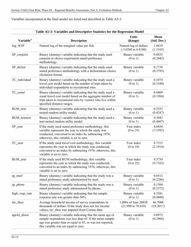
Section 316(b) Final Rule: Phase III – Regional Benefits Assessment, Part A: Evaluation Methods Chapter A5
A5-14
Variables incorporated in the final model are listed and described in Table A5-3.
Table A5-3: Variables and Descriptive Statistics for the Regression Model
VariableP
aP Description
Units (Range)
Mean (Std. Dev.)
log_WTP Natural log of the marginal value per fish. Natural log of dollars (-3.0260 to 6.4180)
1.8419 (1.3165)
SP_conjoint Binary (dummy) variable indicating that the study used conjoint or choice-experiment stated preference methodology.
Binary variable (0 to 1)
0.0435 (0.2042)
SP_dichot Binary (dummy) variable indicating that the study used stated preference methodology with a dichotomous choice elicitation format.
Binary variable (0 to 1)
0.1739 (0.3795)
TC_individual Binary (dummy) variable indicating that the study used a travel cost model based on the number of trips taken by individual respondents to recreational sites.
Binary variable (0 to 1)
0.1074 (0.3100)
TC_zonal Binary (dummy) variable indicating that the study used a zonal travel cost model based on the aggregate number of trips taken to recreational sites by visitors who live within specified distance ranges.
Binary variable (0 to 1)
0.0409 (0.1984)
RUM_nest Binary (dummy) variable indicating that the study used a nested random utility model.
Binary variable (0 to 1)
0.2353 (0.4247)
RUM_nonnest Binary (dummy) variable indicating that the study used a non-nested random utility model.
Binary variable (0 to 1)
0.3043 (0.4607)
SP_year If the study used stated preference methodology, this variable represents the year in which the study was conducted, converted to an index by subtracting 1976; otherwise, this variable is set to zero.
Year index (0 to 25)
4.6036 (7.3592)
TC_year If the study used travel cost methodology, this variable represents the year in which the study was conducted, converted to an index by subtracting 1976; otherwise, this variable is set to zero.
Year index (0 to 18)
0.7315 (2.1914)
RUM_year If the study used RUM methodology, this variable represents the year in which the study was conducted, converted to an index by subtracting 1976; otherwise, this variable is set to zero.
Year index (0 to 25)
9.3734 (9.7162)
sp_mail Binary (dummy) variable indicating that the study was a stated preference study administered by mail.
Binary variable (0 to 1)
0.0512 (0.2206)
sp_phone Binary (dummy) variable indicating that the study was a stated preference study administered by phone.
Binary variable (0 to 1)
0.1304 (0.3372)
high_resp_rate Binary (dummy) variable indicating that the sample response rate was greater than 50%.
Binary variable (0 to 1)
0.3581 (0.4800)
inc_thou Average household income of survey respondents in thousands of dollars. If the study does not list income values, inc_thou was imputed from Census data.
1,000s of June 2003$ (21.990 to 70.610)
46.7008 (10.2017)
age42_down Binary (dummy) variable indicating that the mean age of sample respondents was less than 43. If the mean sample age was greater than or equal to 43, or was not reported, this variable was set equal to zero.
Binary variable (0 to 1)
0.0972 (0.2966)
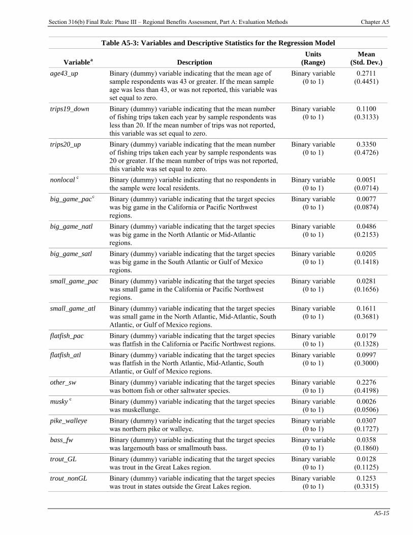
Section 316(b) Final Rule: Phase III – Regional Benefits Assessment, Part A: Evaluation Methods Chapter A5
A5-15
Table A5-3: Variables and Descriptive Statistics for the Regression Model
VariableP
aP Description
Units (Range)
Mean (Std. Dev.)
age43_up Binary (dummy) variable indicating that the mean age of sample respondents was 43 or greater. If the mean sample age was less than 43, or was not reported, this variable was set equal to zero.
Binary variable (0 to 1)
0.2711 (0.4451)
trips19_down Binary (dummy) variable indicating that the mean number of fishing trips taken each year by sample respondents was less than 20. If the mean number of trips was not reported, this variable was set equal to zero.
Binary variable (0 to 1)
0.1100 (0.3133)
trips20_up Binary (dummy) variable indicating that the mean number of fishing trips taken each year by sample respondents was 20 or greater. If the mean number of trips was not reported, this variable was set equal to zero.
Binary variable (0 to 1)
0.3350 (0.4726)
nonlocalP
cP Binary (dummy) variable indicating that no respondents in
the sample were local residents. Binary variable
(0 to 1) 0.0051
(0.0714) big_game_pacP
cP Binary (dummy) variable indicating that the target species
was big game in the California or Pacific Northwest regions.
Binary variable (0 to 1)
0.0077 (0.0874)
big_game_natl Binary (dummy) variable indicating that the target species was big game in the North Atlantic or Mid-Atlantic regions.
Binary variable (0 to 1)
0.0486 (0.2153)
big_game_satl Binary (dummy) variable indicating that the target species was big game in the South Atlantic or Gulf of Mexico regions.
Binary variable (0 to 1)
0.0205 (0.1418)
small_game_pac Binary (dummy) variable indicating that the target species was small game in the California or Pacific Northwest regions.
Binary variable (0 to 1)
0.0281 (0.1656)
small_game_atl Binary (dummy) variable indicating that the target species was small game in the North Atlantic, Mid-Atlantic, South Atlantic, or Gulf of Mexico regions.
Binary variable (0 to 1)
0.1611 (0.3681)
flatfish_pac Binary (dummy) variable indicating that the target species was flatfish in the California or Pacific Northwest regions.
Binary variable (0 to 1)
0.0179 (0.1328)
flatfish_atl Binary (dummy) variable indicating that the target species was flatfish in the North Atlantic, Mid-Atlantic, South Atlantic, or Gulf of Mexico regions.
Binary variable (0 to 1)
0.0997 (0.3000)
other_sw Binary (dummy) variable indicating that the target species was bottom fish or other saltwater species.
Binary variable (0 to 1)
0.2276 (0.4198)
muskyP
cP Binary (dummy) variable indicating that the target species
was muskellunge. Binary variable
(0 to 1) 0.0026
(0.0506) pike_walleye Binary (dummy) variable indicating that the target species
was northern pike or walleye. Binary variable
(0 to 1) 0.0307
(0.1727) bass_fw Binary (dummy) variable indicating that the target species
was largemouth bass or smallmouth bass. Binary variable
(0 to 1) 0.0358
(0.1860) trout_GL Binary (dummy) variable indicating that the target species
was trout in the Great Lakes region. Binary variable
(0 to 1) 0.0128
(0.1125) trout_nonGL Binary (dummy) variable indicating that the target species
was trout in states outside the Great Lakes region. Binary variable
(0 to 1) 0.1253
(0.3315)
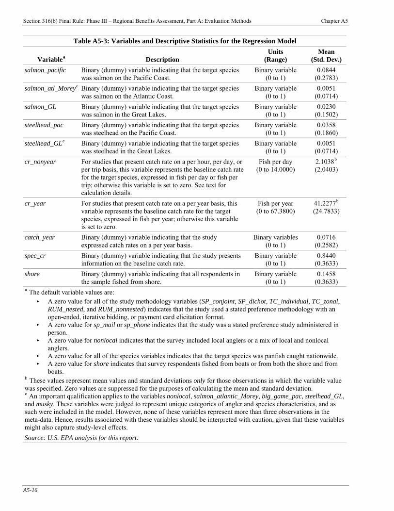
Section 316(b) Final Rule: Phase III – Regional Benefits Assessment, Part A: Evaluation Methods Chapter A5
A5-16
Table A5-3: Variables and Descriptive Statistics for the Regression Model
VariableP
aP Description
Units (Range)
Mean (Std. Dev.)
salmon_pacific Binary (dummy) variable indicating that the target species was salmon on the Pacific Coast.
Binary variable (0 to 1)
0.0844 (0.2783)
salmon_atl_MoreyP
cP Binary (dummy) variable indicating that the target species was salmon on the Atlantic Coast.
Binary variable (0 to 1)
0.0051 (0.0714)
salmon_GL Binary (dummy) variable indicating that the target species was salmon in the Great Lakes.
Binary variable (0 to 1)
0.0230 (0.1502)
steelhead_pac Binary (dummy) variable indicating that the target species was steelhead on the Pacific Coast.
Binary variable (0 to 1)
0.0358 (0.1860)
steelhead_GLP
cP Binary (dummy) variable indicating that the target species
was steelhead in the Great Lakes. Binary variable
(0 to 1) 0.0051
(0.0714) cr_nonyear For studies that present catch rate on a per hour, per day, or
per trip basis, this variable represents the baseline catch rate for the target species, expressed in fish per day or fish per trip; otherwise this variable is set to zero. See text for calculation details.
Fish per day (0 to 14.0000)
2.1038P
bP
(2.0403)
cr_year For studies that present catch rate on a per year basis, this variable represents the baseline catch rate for the target species, expressed in fish per year; otherwise this variable is set to zero.
Fish per year (0 to 67.3800)
41.2277P
bP
(24.7833)
catch_year Binary (dummy) variable indicating that the study expressed catch rates on a per year basis.
Binary variables (0 to 1)
0.0716 (0.2582)
spec_cr Binary (dummy) variable indicating that the study presents information on the baseline catch rate.
Binary variable (0 to 1)
0.8440 (0.3633)
shore Binary (dummy) variable indicating that all respondents in the sample fished from shore.
Binary variable (0 to 1)
0.1458 (0.3633)
P
aP The default variable values are:
< A zero value for all of the study methodology variables (SP_conjoint, SP_dichot, TC_individual, TC_zonal, RUM_nested, and RUM_nonnested) indicates that the study used a stated preference methodology with an open-ended, iterative bidding, or payment card elicitation format.
< A zero value for sp_mail or sp_phone indicates that the study was a stated preference study administered in person.
< A zero value for nonlocal indicates that the survey included local anglers or a mix of local and nonlocal anglers.
< A zero value for all of the species variables indicates that the target species was panfish caught nationwide. < A zero value for shore indicates that survey respondents fished from boats or from both the shore and from
boats. P
bP These values represent mean values and standard deviations only for those observations in which the variable value
was specified. Zero values are suppressed for the purposes of calculating the mean and standard deviation. P
cP An important qualification applies to the variables nonlocal, salmon_atlantic_Morey, big_game_pac, steelhead_GL,
and musky. These variables were judged to represent unique categories of angler and species characteristics, and as such were included in the model. However, none of these variables represent more than three observations in the meta-data. Hence, results associated with these variables should be interpreted with caution, given that these variables might also capture study-level effects. Source: U.S. EPA analysis for this report.
Section 316(b) Final Rule: Phase III – Regional Benefits Assessment, Part A: Evaluation Methods Chapter A5
A5-17
A5-3.2 Model and Results a. Model Past meta-analyses have incorporated a range of different statistical methods, with none universally accepted as superior (e.g., Santos, 1998; Poole and Greenland, 1999; Poe et al., 2001; Bateman and Jones, 2003). Nonetheless, there is general consensus that certain statistical issues should be addressed during model development. For example, many researchers agree that models must somehow address potential correlation among observations provided by like authors or studies and the related potential for heteroskedasticity (Rosenberger and Loomis, 2000b; Bateman and Jones, 2003; Johnston et al., 2003). This meta-analysis model is estimated following standard methods illustrated in the most recent literature, recognizing that there are some areas in which the literature provides mixed guidance (e.g., the use of weighting). EPA followed recent work by Bateman and Jones (2003) in applying a multilevel model specification to the meta-data to address potential correlation among observations gathered from single studies. Multilevel (or hierarchical) models may be estimated as either random-effects or random-coefficients models, and are described in detail elsewhere (Goldstein, 1995; Singer, 1998). The fundamental distinction between these models and classical linear models is the two-part modeling of the equation error to account for hierarchical data. Here, the meta-data are comprised of multiple observations per valuation survey (i.e., all observations from studies that were based on a common survey), and there is a corresponding possibility of correlated errors among observations that share a common survey.PF
6FP
The common approach to modeling such potential correlation is to divide the residual variance of estimates into two parts: a random error that is independently and identically distributed (iid) across all observations, and a random effect that represents systematic variation related to each survey. The model is estimated as a two-level hierarchy, with level one corresponding to marginal value per fish estimates (individual observations), and level two corresponding to individual surveys. The random effect may be interpreted as a deviation from the mean equation intercept associated with individual surveys (Bateman and Jones, 2003). The model is estimated using a maximum likelihood estimator (MLE), based on the assumption that random effects are distributed multivariate normal. Following the arguments of Bateman and Jones (2003), observations are unweighted. Also following prior work (e.g., Smith and Osborne, 1996; Poe et al., 2001), covariances are obtained using the Huber-White covariance estimator. As described by Smith and Osborne (1996, p. 293), “this approach treats each study as the equivalent of a sample cluster with the potential for heteroskedasticity . . . across clusters” (Smith and Osborne, 1996). Random effects models such as the multilevel model applied here are increasingly becoming standard in resource economics applications, and are estimable using a variety of readily available software packages. For comparison, models were also estimated using both ordinary least squares (OLS) and weighted least squares (WLS) with robust variance estimation and multilevel models with standard (non-robust) variance estimation. Although the OLS RP
2P value was somewhat better than the illustrated model, the significance of the individual variable
coefficients was highest in the illustrated model. As noted in section A5-3.1, the dependent variable in the regression is the log of WTP per fish, and the independent variables are all linear, resulting in a semi-log functional form. This functional form has advantages because of: (1) its fit to the data, (2) the intuitive results provided by the functional form, and (3) the common use of this functional form in the meta-analysis literature (e.g., Smith and Osborne, 1996; Santos, 1998). While linear forms are also common in the literature (Rosenberger and Loomis, 2000a,b; Poe et al., 2001; Bateman and Jones, 2003), specifications requiring more intensive data transformations (e.g., Box-Cox, log-log) are less common. Given questions about a priori restrictions on the functional form, final decisions regarding functional forms were made based on a combination of general principles and empirical performance. The semi-log model was chosen
P
6P EPA chose to group observations by valuation survey rather than by study or author because in a number of
cases, studies based on the same survey produce similar results, even if written by different authors.
Section 316(b) Final Rule: Phase III – Regional Benefits Assessment, Part A: Evaluation Methods Chapter A5
A5-18
over the linear model based on the ability of the semi-log form to capture curvature in the valuation function and its improved fit to the data. It also allows independent variables to influence WTP (after transformation from its natural log) in a multiplicative rather than additive manner. ˜ A note on model specification Following standard econometric practice, the final model is specified based on guidance from theory and prior literature. For example, Arrow et al. (1993) make a fundamental distinction between discrete choice and open-ended payment mechanisms (where open-ended include iterative bidding, payment cards, etc.). Hence, this is the distinction made in the final model (i.e., including the variables SP_conjoint and SP_dichot). Similarly, other methodology variables in the model were chosen based on theoretical considerations and prior findings in the literature (e.g., nested RUM vs. non-nested RUM; mail surveys vs. phone vs. in-person surveys). As is common in meta-analysis, some variables were excluded from the model because sufficient data were incomplete or missing from most studies in the meta-data. For example, a variable characterizing the average number of years respondents had been fishing was excluded because too few observations were available. Some other variables were also excluded because of a clear lack of statistical significance in all estimated models. For example, if there was no overriding theoretical or other rationale for retaining the variable in the model, and the variable was clearly insignificant, EPA excluded the variable from the model. For example, variables representing gender, survey size, and estimate size were dropped because they added no significant explanatory power to the model. However, certain variables were retained in the model for theoretical reasons, even if significance levels were low. Such specification of meta-analysis models using a combination of theoretical guidance and empirical considerations is standard in modeling efforts. b. Results Table A5-4 presents the results of the model.
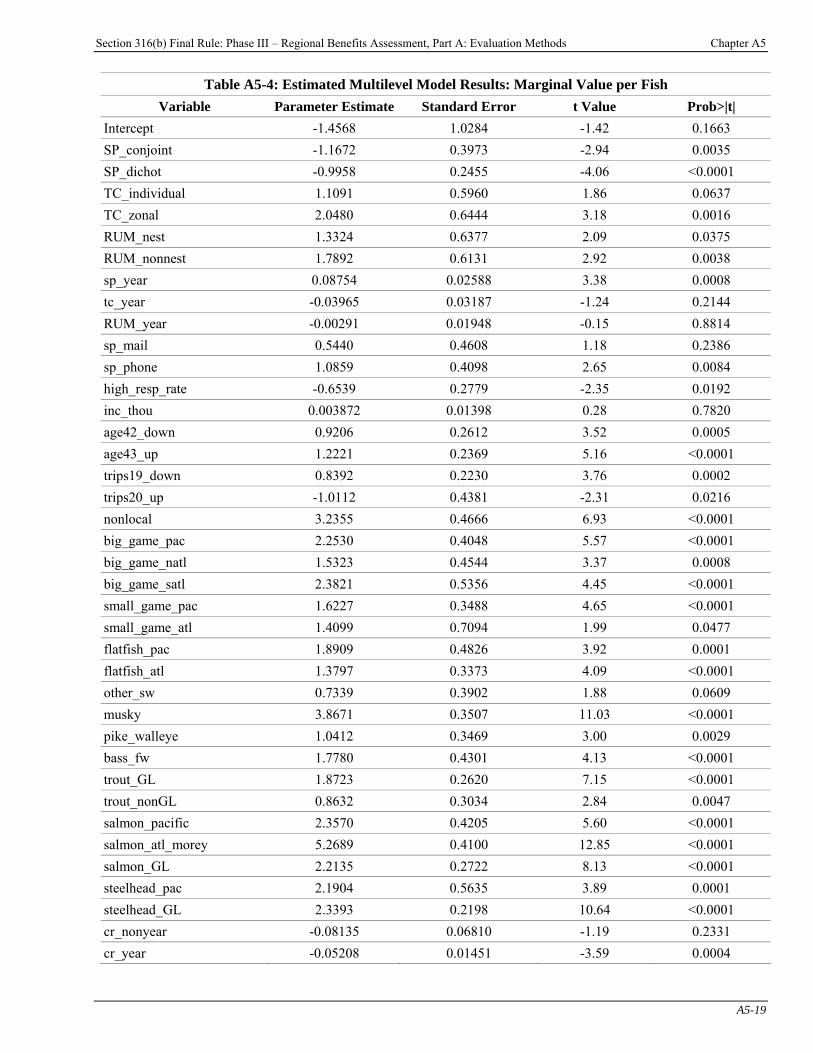
Section 316(b) Final Rule: Phase III – Regional Benefits Assessment, Part A: Evaluation Methods Chapter A5
A5-19
Table A5-4: Estimated Multilevel Model Results: Marginal Value per Fish Variable Parameter Estimate Standard Error t Value Prob>|t|
Intercept -1.4568 1.0284 -1.42 0.1663 SP_conjoint -1.1672 0.3973 -2.94 0.0035 SP_dichot -0.9958 0.2455 -4.06 <0.0001 TC_individual 1.1091 0.5960 1.86 0.0637 TC_zonal 2.0480 0.6444 3.18 0.0016 RUM_nest 1.3324 0.6377 2.09 0.0375 RUM_nonnest 1.7892 0.6131 2.92 0.0038 sp_year 0.08754 0.02588 3.38 0.0008 tc_year -0.03965 0.03187 -1.24 0.2144 RUM_year -0.00291 0.01948 -0.15 0.8814 sp_mail 0.5440 0.4608 1.18 0.2386 sp_phone 1.0859 0.4098 2.65 0.0084 high_resp_rate -0.6539 0.2779 -2.35 0.0192 inc_thou 0.003872 0.01398 0.28 0.7820 age42_down 0.9206 0.2612 3.52 0.0005 age43_up 1.2221 0.2369 5.16 <0.0001 trips19_down 0.8392 0.2230 3.76 0.0002 trips20_up -1.0112 0.4381 -2.31 0.0216 nonlocal 3.2355 0.4666 6.93 <0.0001 big_game_pac 2.2530 0.4048 5.57 <0.0001 big_game_natl 1.5323 0.4544 3.37 0.0008 big_game_satl 2.3821 0.5356 4.45 <0.0001 small_game_pac 1.6227 0.3488 4.65 <0.0001 small_game_atl 1.4099 0.7094 1.99 0.0477 flatfish_pac 1.8909 0.4826 3.92 0.0001 flatfish_atl 1.3797 0.3373 4.09 <0.0001 other_sw 0.7339 0.3902 1.88 0.0609 musky 3.8671 0.3507 11.03 <0.0001 pike_walleye 1.0412 0.3469 3.00 0.0029 bass_fw 1.7780 0.4301 4.13 <0.0001 trout_GL 1.8723 0.2620 7.15 <0.0001 trout_nonGL 0.8632 0.3034 2.84 0.0047 salmon_pacific 2.3570 0.4205 5.60 <0.0001 salmon_atl_morey 5.2689 0.4100 12.85 <0.0001 salmon_GL 2.2135 0.2722 8.13 <0.0001 steelhead_pac 2.1904 0.5635 3.89 0.0001 steelhead_GL 2.3393 0.2198 10.64 <0.0001 cr_nonyear -0.08135 0.06810 -1.19 0.2331 cr_year -0.05208 0.01451 -3.59 0.0004
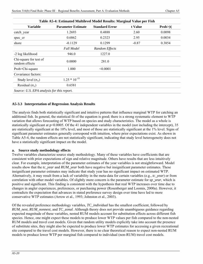
Section 316(b) Final Rule: Phase III – Regional Benefits Assessment, Part A: Evaluation Methods Chapter A5
A5-20
Table A5-4: Estimated Multilevel Model Results: Marginal Value per Fish Variable Parameter Estimate Standard Error t Value Prob>|t|
catch_year 1.2693 0.4888 2.60 0.0098 spec_cr 0.6862 0.2323 2.95 0.0034 shore -0.1129 0.1299 -0.87 0.3854 Full Model Random Effects -2 log likelihood 946.0 1227.0 Chi-square for test of random effects 0.0000 281.0
Prob>Chi-square 1.000 <0.0001 Covariance factors:
Study level (σBuB) 1.25 * 10P
-19P
Residual (σBeB) 0.6581 Source: U.S. EPA analysis for this report.
A5-3.3 Interpretation of Regression Analysis Results The analysis finds both statistically significant and intuitive patterns that influence marginal WTP for catching an additional fish. In general, the statistical fit of the equation is good; there is a strong systematic element to WTP variation that allows forecasting of WTP based on species and study characteristics. The model as a whole is statistically significant at p<0.0005. Of the 41 independent variables in the model (not including the intercept), 35 are statistically significant at the 10% level, and most of those are statistically significant at the 1% level. Signs of significant parameter estimates generally correspond with intuition, where prior expectations exist. As shown in Table A5-4, the random effects are not statistically significant, indicating that study level heterogeneity does not have a statistically significant impact on the model. a. Source study methodology effects Twelve variables characterize source study methodology. Many of these variables have coefficients that are consistent with prior expectations of sign and relative magnitude. Others have results that are less intuitively clear. For example, interpretation of the parameter estimates of the year variables is not straightforward. Model results show that the tc_year and RUM_year both have negative but insignificant parameter estimates. These insignificant parameter estimates may indicate that study year has no significant impact on estimated WTP. Alternatively, it may result from a lack of variability in the meta-data for certain variables (e.g., tc_year) or from correlation with other model variables. Of slightly more concern is the parameter estimate for sp_year, which is positive and significant. This finding is consistent with the hypothesis that real WTP increases over time due to changes in angler experiences, preferences, or purchasing power (Rosenberger and Loomis, 2000a). However, it contradicts the expectation that advances in stated preference survey design over time have led to more conservative WTP estimates (Arrow et al., 1993; Johnston et al., 2003). Of the revealed preference methodology variables, TC_individual has the smallest coefficient, followed by RUM_nest, RUM_nonnest, and TC_zonal. Although theory does not provide unambiguous guidance regarding expected magnitude of these variables, nested RUM models account for substitution effects across different fish species. Hence, one might expect these models to produce lower WTP values per fish compared to the non-nested RUM models and travel cost models. Given that random utility models explicitly take into account the presence of substitute sites, they might also be expected to produce lower WTP estimates for accessing a given recreational site compared to the travel cost models. However, there is no clear theoretical reason to expect non-nested RUM models to produce lower WTP per marginal fish compared to individual (non-RUM) travel cost models.
Section 316(b) Final Rule: Phase III – Regional Benefits Assessment, Part A: Evaluation Methods Chapter A5
A5-21
The stated preference dummy variables (SP_conjoint, SP_dichot, and the default value, SP_other) have much lower coefficients than the travel cost and random utility model variables. This finding is consistent with past research by Cameron (1992) and others, who demonstrate that stated preference methods can produce lower estimates of direct use values for the same quality change than revealed preference methods. However, interpretation of the methodology variables associated with the stated preference approaches is confounded by the large positive coefficient on sp_year, which indicates that among more recent studies, revealed preference methods may produce higher estimates of WTP per additional fish. Of the remaining three methodology variables, two are significant. The variable sp_phone has a significantly positive coefficient, indicating that phone interview methods tend to yield higher WTP values than in-person interview methods. The variable sp_mail was retained in the meta-analysis for theoretical reasons, despite its lack of statistical significance. The parameter estimate of the binary variable high_response_rate is negative and significant (p<0.05), a finding consistent with prior expectations. b. Sample characteristics effects Six variables characterize demographic and economic attributes. Five of the associated parameter estimates are statistically significant at p<0.05, and most have expected signs. Model results show that respondents with higher incomes (inc_thou) are willing to pay more to catch an additional fish per trip — an expected result. The parameter estimate on age42_down is less than the parameter estimate on age43_up, suggesting that older anglers may be willing to pay more to catch an additional fish. Insofar as age is correlated with income, the difference between these variables may be capturing the effects of increased angler income. However, this result is not entirely intuitive, since older anglers may have more experience and are therefore likely to have better success rates. Thus, they might not be willing to pay as much to catch additional fish, due to diminishing marginal WTP per fish caught. The parameter estimate for trips19_down is much larger than the parameter estimate for trips20_up, indicating that anglers who take more fishing trips per year (and who presumably catch more fish during the fishing season) have lower marginal values per fish than anglers who take fewer trips per year. This is not surprising, since catching an additional fish during a single trip increases total seasonal catch for avid anglers by a smaller percentage than for anglers who fish less often. Moreover, those taking a greater number of trips, and presumably catching more fish, might be expected to have a somewhat diminished WTP for an additional fish, again based on the concept of diminishing marginal utility. The parameter estimate for the nonlocal variable is positive and significant (p<0.0001) indicating that anglers who travel out of state to fish are willing to pay much more to catch additional fish than local residents. However, this effect should be interpreted in the context of the underlying data. This variable is based on only two observations and reflects values of anglers who travel long distances (e.g., visit Alaska) to their fishing destinations.PF
7FP Hence, EPA suggests that results for this variable may not be readily generalizable.
c. Species targeted effects The model includes 18 binary variables that characterize the target species and region in which the species was targeted. All but one of these variables have coefficients that are significant at p<0.05. The variables can be divided into three general groups: marine species, freshwater species, and salmonoids. In general, the sign and magnitude of the coefficients of most of the variables are consistent with prior expectations regarding both the relative worth of different species and the relative worth of individual species in different geographic regions. However, unlike other variables, these expectations are based on existing literature, prior empirical results, and anecdotal evidence, rather than economic theory.
P
7P In alternative model specifications, EPA was not able to find a statistically significant difference between the
variables local (representing survey samples that included only local residents) and local_nonlocal (representing survey samples that included a mix of local and nonlocal residents).
Section 316(b) Final Rule: Phase III – Regional Benefits Assessment, Part A: Evaluation Methods Chapter A5
A5-22
Of the marine species variables, big_game_pac and big_game_satl have the largest magnitude. Big_game_natl has a somewhat lower coefficient, which is likely due to a somewhat different species composition in the big game category in the North Atlantic and Mid-Atlantic regions. Small_game_atl has a slightly smaller coefficient than small_game_pac, and flatfish_atl has a lower coefficient than flatfish_pac, but these differences are not statistically significant. As expected, the other_sw variable, which includes bottomfish, smelt, grunion, and other miscellaneous saltwater species, has a relatively small coefficient compared to the other marine species. Results for the freshwater variables also meet prior expectations. Among warmwater species, musky has the highest coefficient, followed by trout_GL and bass_fw. These results are expected, given that muskellunge are relatively rare and generally grow much larger than other fish in the pike family (pike_walleye), and trout caught in the Great Lakes are often much larger than trout caught in smaller rivers and lakes (trout_nonGL). The default value for the regression is panfish, which includes species such as catfish, and perch. Regression results indicate that the value of catching an additional fish of these species is significantly lower than the other species. The coefficients of the salmon and steelhead variables are fairly large. These findings are consistent with the popularity of salmonoids as game fish. Salmon_atlantic_Morey has a very large coefficient, but this variable is based on observations from only one study — hence results for this variable should be interpreted accordingly.PF
8FP
Salmon_GL has a lower coefficient than salmon_pacific, which is consistent with the larger size of Pacific salmon. Steelhead_GL has a slightly higher coefficient than either steelhead_pac or salmon_GL. d. Angling characteristics The angling characteristics variables include two catch rate variables (cr_nonyear and cr_year), two dummy variable indicating whether catch rates were specified (spec_cr) and what units were used (catch_year), and a fishing mode variable (shore). The negative parameter estimates on both cr_nonyear and cr_year indicate that anglers’ WTP for catching an additional fish per trip decreases as the number of fish already caught increases.PF
9FP
This result is consistent with both economic theory and prior expectations. The parameter estimate on the shore variable is negative but insignificant. e. Model limitations Although the meta-analysis results presented in the previous section indicate that the model’s statistical fit is quite good, EPA notes that there are a number of limitations and uncertainties involved in the estimation and results of the model. These limitations stem largely from the quality and quantity of information available from the original studies, and from the statistical methods used to estimate the model. First of all, regardless of the explanatory power of the meta-analysis regression equation, the model is only as good as the data upon which it is based. EPA believes that WTP per fish estimates from the 24 peer-reviewed journal articles are based on careful, high quality research. The data set also includes estimates from 24 reports, dissertations, academic working papers, and books, which may or may not be subject to the same academic scrutiny and quality standards. Nonetheless, based on EPA’s review of these documents, the Agency believes that all of the estimates included in the data set are of reasonable academic quality. Another limitation of the data is that some demographic and other variables are present for only a subset of the meta-observations. For example, the variables age and trips have a large number of missing observations, indicating that the original studies do not always provide detailed demographic data. By specifying variables to indicate missing observations (missing observations are indicated by zero values for both age42_down and age43_up, and for both trips19_down and trips20_up), EPA was able to control for the missing data. This
P
8P The study was based on Atlantic salmon fishing in Maine in 1988. Angling for Atlantic salmon is currently
illegal in Maine (MaineToday.com, 2003).
P
9P Although cr_nonyear lacks significance (p<0.32), this variable is consistently negative across a variety of model
specifications.
Section 316(b) Final Rule: Phase III – Regional Benefits Assessment, Part A: Evaluation Methods Chapter A5
A5-23
specification presumes that a fixed shift in intercept (i.e., using a dummy variable) is sufficient to control for systematic differences associated with the lack of data for specific variables — an unverifiable assumption. Moreover, the significance of these variables would be clearer if more observations were available. A third limitation of the data, related to variable specification, is the imperfect match between the aggregate species variables specified in the model and the species evaluated in each individual study. Although in most cases the match was good, some studies provided WTP per fish estimates for very broad categories of species, such as “bottomfish (flounder family, cod family, snapper, grouper, jack, grunt, sea bass, porgy, wreckfish)” (Schuhmann, 1998). EPA assigned these estimates to the aggregate species group variable that most closely matched the largest number of species from the list provided in the study, but the Agency acknowledges that this process introduces uncertainty into the analysis. Another source of uncertainty related to the species groupings is that creating variables for aggregate species groups reduces the precision of the resulting benefit estimates. By aggregating species into categories, EPA was able to improve the fit of the meta-analysis model, but this aggregation also results in a lower level of detail in the values that can be predicted. In particular, the panfish, other saltwater, and big game categories include relatively diverse species. Model results are also subject to choices regarding functional form and statistical approach, although many of the primary model effects are robust to reasonable changes in functional form and/or statistical methods. The rationale for the specific functional form and model structure chosen is detailed above in section A5-3.2a. In general, meta-analysis may provide a superior alternative to the calculation and use of a simple arithmetic mean, as it allows WTP to be adjusted to account for the characteristics of the transfer site. The model’s ability to adjust WTP appropriately is suggested by the many systematic (statistically significant) patterns revealed by the meta-analysis regression. Nonetheless, the use and interpretation of meta-analysis models for benefit transfer, and the use of benefit transfer in general, are subject to the constraints and concerns expressed elsewhere in the literature (e.g., Desvousges et al., 1998; Poe et al., 2001; Vandenberg et al., 2001). A5-4 Application of the Meta-Analysis Results to the Analysis of Recreational Benefits of
the Section 316(b) Regulatory Analysis Options for Phase III Facilities The results of the meta-analysis in conjunction with information specific to the resource users and populations of species that will benefit from reduced I&E can be used to estimate the recreational welfare gain associated with the section 316(b) regulatory analysis options for Phase III facilities. This analysis involves the following steps:
< estimating the marginal recreational value per fish for each species affected by each respective analysis option in each region;
< calculating the recreational fishing benefits from eliminating baseline I&E losses, by multiplying the marginal value per fish by the number of recreational fish currently lost to I&E that would otherwise be caught by recreational anglers; and
< calculating the recreational fishing benefits from the regulatory analysis options for Phase III facilities, by multiplying the marginal value per fish by the number of additional fish that would be caught by recreational anglers because of reduced I&E losses of recreational fish.
A5-4.1 Estimating Marginal Value per Fish EPA used the estimated meta-regression to estimate marginal values per fish for the species affected by I&E at Phase III facilities. To calculate the marginal value per fish for the affected species, EPA chose input values for the independent variables based on the affected species characteristics, study regions, and demographic characteristics of the affected angling populations. The study design variables were selected based on current economic literature. Table A5-5 summarizes the input values for each of the variables in the model.
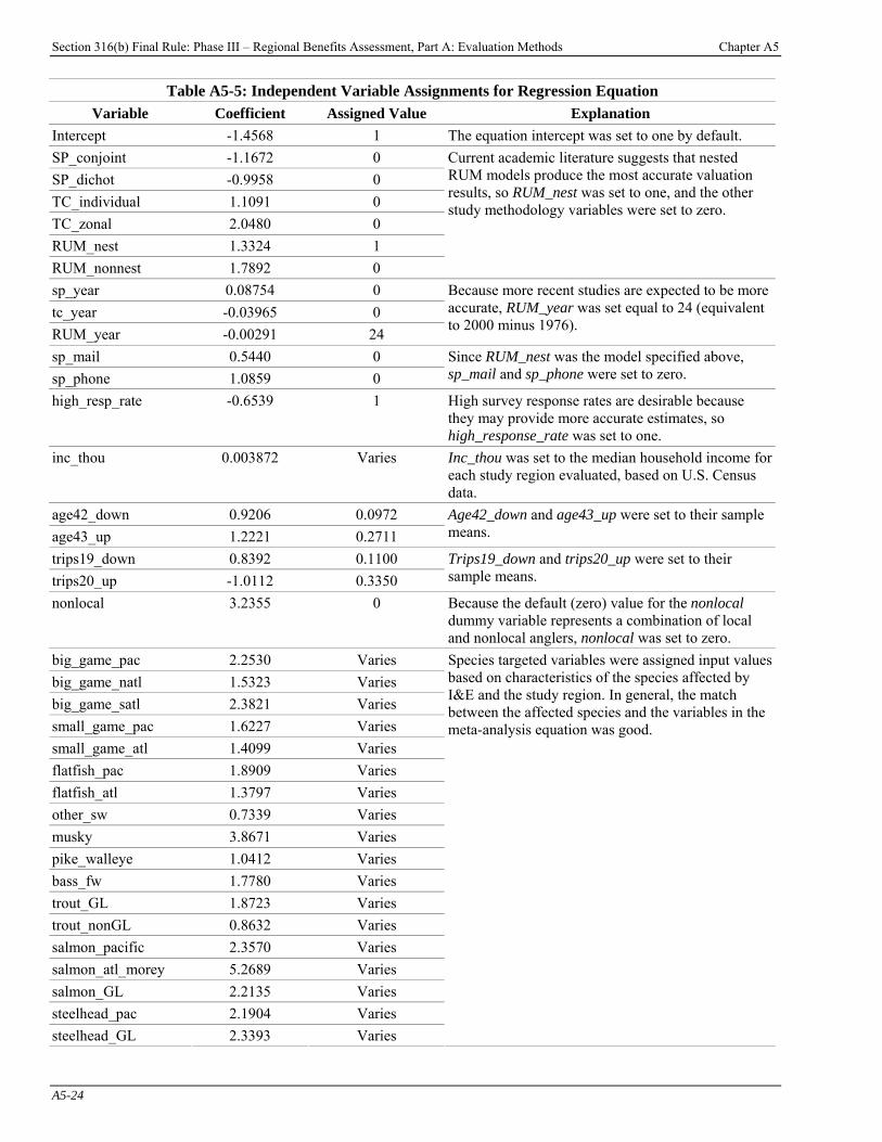
Section 316(b) Final Rule: Phase III – Regional Benefits Assessment, Part A: Evaluation Methods Chapter A5
A5-24
Table A5-5: Independent Variable Assignments for Regression Equation Variable Coefficient Assigned Value Explanation
Intercept -1.4568 1 The equation intercept was set to one by default. SP_conjoint -1.1672 0 SP_dichot -0.9958 0 TC_individual 1.1091 0 TC_zonal 2.0480 0 RUM_nest 1.3324 1 RUM_nonnest 1.7892 0
Current academic literature suggests that nested RUM models produce the most accurate valuation results, so RUM_nest was set to one, and the other study methodology variables were set to zero.
sp_year 0.08754 0 tc_year -0.03965 0 RUM_year -0.00291 24
Because more recent studies are expected to be more accurate, RUM_year was set equal to 24 (equivalent to 2000 minus 1976).
sp_mail 0.5440 0 sp_phone 1.0859 0
Since RUM_nest was the model specified above, sp_mail and sp_phone were set to zero.
high_resp_rate -0.6539 1 High survey response rates are desirable because they may provide more accurate estimates, so high_response_rate was set to one.
inc_thou 0.003872 Varies Inc_thou was set to the median household income for each study region evaluated, based on U.S. Census data.
age42_down 0.9206 0.0972 age43_up 1.2221 0.2711
Age42_down and age43_up were set to their sample means.
trips19_down 0.8392 0.1100 trips20_up -1.0112 0.3350
Trips19_down and trips20_up were set to their sample means.
nonlocal 3.2355 0 Because the default (zero) value for the nonlocal dummy variable represents a combination of local and nonlocal anglers, nonlocal was set to zero.
big_game_pac 2.2530 Varies big_game_natl 1.5323 Varies big_game_satl 2.3821 Varies small_game_pac 1.6227 Varies small_game_atl 1.4099 Varies flatfish_pac 1.8909 Varies flatfish_atl 1.3797 Varies other_sw 0.7339 Varies musky 3.8671 Varies pike_walleye 1.0412 Varies bass_fw 1.7780 Varies trout_GL 1.8723 Varies trout_nonGL 0.8632 Varies salmon_pacific 2.3570 Varies salmon_atl_morey 5.2689 Varies salmon_GL 2.2135 Varies steelhead_pac 2.1904 Varies steelhead_GL 2.3393 Varies
Species targeted variables were assigned input values based on characteristics of the species affected by I&E and the study region. In general, the match between the affected species and the variables in the meta-analysis equation was good.
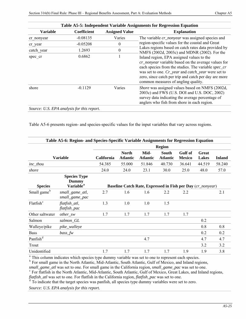
Section 316(b) Final Rule: Phase III – Regional Benefits Assessment, Part A: Evaluation Methods Chapter A5
A5-25
Table A5-5: Independent Variable Assignments for Regression Equation Variable Coefficient Assigned Value Explanation
cr_nonyear -0.08135 Varies cr_year -0.05208 0 catch_year 1.2693 0 spec_cr 0.6862 1
The variable cr_nonyear was assigned species and region-specific values for the coastal and Great Lakes regions based on catch rates data provided by NMFS (2002d, 2003c) and MDNR (2002). For the Inland region, EPA assigned values to the cr_nonyear variable based on the average values for each species from the studies. The variable spec_cr was set to one. Cr_year and catch_year were set to zero, since catch per trip and catch per day are more common measures of angling quality.
shore -0.1129 Varies Shore was assigned values based on NMFS (2002d, 2003c) and FWS (U.S. DOI and U.S. DOC, 2002) survey data indicating the average percentage of anglers who fish from shore in each region.
Source: U.S. EPA analysis for this report. Table A5-6 presents region- and species-specific values for the input variables that vary across regions.
Table A5-6: Region- and Species-Specific Variable Assignments for Regression Equation Region
Variable California North
Atlantic Mid-
Atlantic South
Atlantic Gulf of Mexico
Great Lakes Inland
inc_thou 54.385 55.000 51.846 40.730 36.641 44.519 58.240 shore 24.0 24.0 23.1 30.0 25.0 48.0 57.0
Species
Species Type Dummy
VariableP
aP Baseline Catch Rate, Expressed in Fish per Day (cr_nonyear)
Small gameP
bP small_game_atl,
small_game_pac 2.7 1.6 1.6 2.2 2.2 2.1
FlatfishP
cP flatfish_atl,
flatfish_pac 1.3 1.0 1.0 1.5
Other saltwater other_sw 1.7 1.7 1.7 1.7 1.7 Salmon salmon_GL 0.2 Walleye/pike pike_walleye 0.8 0.8 Bass bass_fw 0.2 0.2 PanfishP
dP 4.7 4.7 4.7
Trout 3.2 3.2 Unidentified 1.7 1.7 1.7 1.7 1.9 1.9 3.8 P
aP This column indicates which species type dummy variable was set to one to represent each species.
P
bP For small game in the North Atlantic, Mid-Atlantic, South Atlantic, Gulf of Mexico, and Inland regions,
small_game_atl was set to one. For small game in the California region, small_game_pac was set to one. P
cP For flatfish in the North Atlantic, Mid-Atlantic, South Atlantic, Gulf of Mexico, Great Lakes, and Inland regions,
flatfish_atl was set to one. For flatfish in the California region, flatfish_pac was set to one. P
dP To indicate that the target species was panfish, all species type dummy variables were set to zero.
Source: U.S. EPA analysis for this report.

Section 316(b) Final Rule: Phase III – Regional Benefits Assessment, Part A: Evaluation Methods Chapter A5
A5-26
EPA decided not to include the error term when using the regression equation to predict marginal values per fish. Bockstael and Strand (1987) argue that if the source of econometric error in an equation is primarily due to omitted variables, the error term should be included, but if the error is primarily due to random preferences, it should be excluded. Because the error term is positive, the empirical effect of including this term is to increase the predicted marginal values. Therefore, EPA’s approach results in more conservative estimates. The Agency also notes that when the error term is excluded, the values predicted by the regression equation are more consistent with those from the underlying studies. Table A5-7 presents the estimated marginal value per fish for all species that were affected by I&E in each region.
Table A5-7: Marginal Recreational Value per Fish, by Region and SpeciesP
aP
Species California North
Atlantic Mid-AtlanticSouth
Atlantic Gulf of Mexico
Great Lakes Inland
Small game $6.11 $5.00 $4.97 $4.82 $4.74 $4.51 Flatfish $8.22 $5.02 $4.73 $4.73 Other saltwater $2.49 $2.51 $2.46 $2.40 $2.34 Salmon $11.17 Walleye/pike $3.46 $3.45 Bass $7.21 $7.59 Panfish $0.89 $1.12 $0.89 Trout $7.94 $2.38 Unidentified $2.61 $2.53 $2.73 $2.41 $3.08 $5.24 $1.88 P
aP All values are in 2004$.
Source: U.S. EPA analysis for this report. A5-4.2 Calculating Recreational Benefits EPA estimated the recreational welfare gain from eliminating current I&E losses and the recreational welfare gain from the regulatory analysis options by combining estimates of the marginal value per fish with estimates of the baseline level of I&E and the reduction in recreational fishing losses from I&E attributable to each analysis option. To calculate the recreational welfare gain from eliminating current I&E losses, EPA multiplied the marginal value per fish by the number of fish that are currently lost due to I&E that would otherwise be caught by recreational anglers. To calculate the recreational welfare gain from each analysis option, EPA multiplied the marginal value per fish by the additional number of fish caught by recreational anglers that would have been impinged or entrained in the absence of the regulation. In these calculations, recreational fish losses are expressed as the number of mature, catchable adults, not as age-1 equivalents so as to not overstate the increase in catch. The results of these calculations are presented in detail in Chapters B4 through H4 of this report. A5-5 Limitations and Uncertainties A number of issues are common to all benefit transfers. Benefit transfer involves adapting research conducted for another purpose to address the policy questions at hand. Because benefits analysis of environmental regulations rarely affords sufficient time to develop original stated preference surveys that are specific to the policy effects, benefit transfer is often the only option to inform a policy decision. Specific issues associated with the estimated regression model and the underlying studies are discussed in section A5-3.3. Additional limitations and uncertainties associated with implementation of the meta-analysis approach are addressed below.
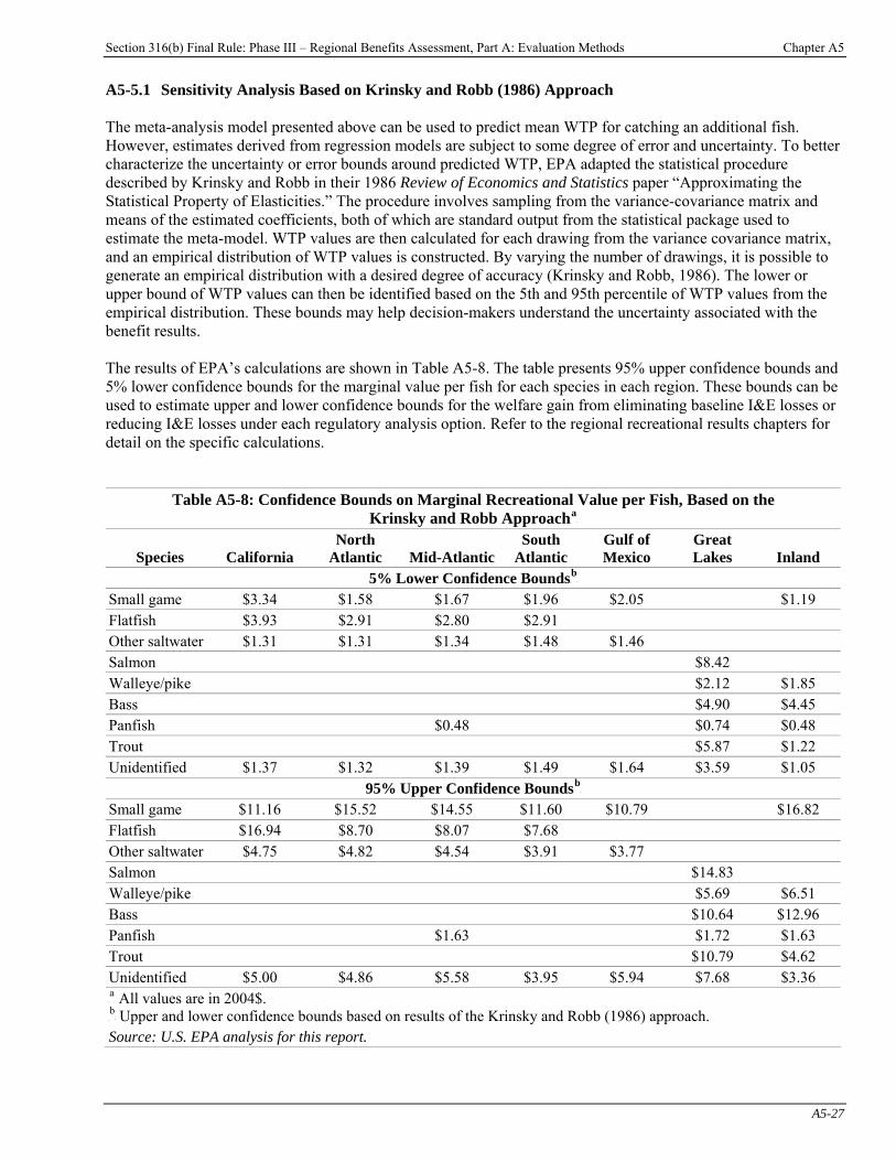
Section 316(b) Final Rule: Phase III – Regional Benefits Assessment, Part A: Evaluation Methods Chapter A5
A5-27
A5-5.1 Sensitivity Analysis Based on Krinsky and Robb (1986) Approach The meta-analysis model presented above can be used to predict mean WTP for catching an additional fish. However, estimates derived from regression models are subject to some degree of error and uncertainty. To better characterize the uncertainty or error bounds around predicted WTP, EPA adapted the statistical procedure described by Krinsky and Robb in their 1986 Review of Economics and Statistics paper “Approximating the Statistical Property of Elasticities.” The procedure involves sampling from the variance-covariance matrix and means of the estimated coefficients, both of which are standard output from the statistical package used to estimate the meta-model. WTP values are then calculated for each drawing from the variance covariance matrix, and an empirical distribution of WTP values is constructed. By varying the number of drawings, it is possible to generate an empirical distribution with a desired degree of accuracy (Krinsky and Robb, 1986). The lower or upper bound of WTP values can then be identified based on the 5th and 95th percentile of WTP values from the empirical distribution. These bounds may help decision-makers understand the uncertainty associated with the benefit results. The results of EPA’s calculations are shown in Table A5-8. The table presents 95% upper confidence bounds and 5% lower confidence bounds for the marginal value per fish for each species in each region. These bounds can be used to estimate upper and lower confidence bounds for the welfare gain from eliminating baseline I&E losses or reducing I&E losses under each regulatory analysis option. Refer to the regional recreational results chapters for detail on the specific calculations.
Table A5-8: Confidence Bounds on Marginal Recreational Value per Fish, Based on the Krinsky and Robb ApproachP
aP
Species California North
Atlantic Mid-AtlanticSouth
Atlantic Gulf of Mexico
Great Lakes Inland
5% Lower Confidence BoundsP
bP
Small game $3.34 $1.58 $1.67 $1.96 $2.05 $1.19 Flatfish $3.93 $2.91 $2.80 $2.91 Other saltwater $1.31 $1.31 $1.34 $1.48 $1.46 Salmon $8.42 Walleye/pike $2.12 $1.85 Bass $4.90 $4.45 Panfish $0.48 $0.74 $0.48 Trout $5.87 $1.22 Unidentified $1.37 $1.32 $1.39 $1.49 $1.64 $3.59 $1.05
95% Upper Confidence BoundsP
bP
Small game $11.16 $15.52 $14.55 $11.60 $10.79 $16.82 Flatfish $16.94 $8.70 $8.07 $7.68 Other saltwater $4.75 $4.82 $4.54 $3.91 $3.77 Salmon $14.83 Walleye/pike $5.69 $6.51 Bass $10.64 $12.96 Panfish $1.63 $1.72 $1.63 Trout $10.79 $4.62 Unidentified $5.00 $4.86 $5.58 $3.95 $5.94 $7.68 $3.36 P
aP All values are in 2004$.
P
bP Upper and lower confidence bounds based on results of the Krinsky and Robb (1986) approach.
Source: U.S. EPA analysis for this report.
Section 316(b) Final Rule: Phase III – Regional Benefits Assessment, Part A: Evaluation Methods Chapter A5
A5-28
A5-5.2 Variable Assignments for Independent Regressors The per fish values estimated from the model depend on the values of the input variables in the meta-analysis. EPA assigned values to the input variables based on established economic theory and characteristics of the affected species and regions. However, because the input values for some variables are uncertain, the resulting per fish values and benefits estimates also include some degree of uncertainty. A5-5.3 Other Limitations and Uncertainties In addition to the limitations and uncertainties involved with the study data and model estimation, which are discussed in section A5-3.3e, there are limitations and uncertainties involved with the calculation of per fish values from the model, and with the use of those values to estimate the welfare gain resulting from the regulatory analysis options considered for the 316(b) regulation. The validity and reliability of benefit transfer — including that based on meta-analysis — depends on a variety of factors. While benefit transfer can provide valid measures of use benefits, tests of its performance have provided mixed results (e.g., Desvousges et al., 1998; Vandenberg et al., 2001; Smith et al., 2002). Nonetheless, benefit transfers are increasingly applied as a core component of benefit cost analyses conducted by EPA and other government agencies (Bergstrom and De Civita, 1999; Griffiths, Undated). Smith et al. (2002, p. 134) state that “nearly all benefit cost analyses rely on benefit transfers, whether they acknowledge it or not.” Given the increasing [or as Smith et al. (2002) might argue, universal] use of benefit transfers, an increasing focus is on the empirical properties of applied transfer methods and models. An important factor in any benefit transfer is the ability of the study site or estimated valuation equation to approximate the resource and context under which benefit estimates are desired. As is common, the meta-analysis model presented here provides a close but not perfect match to the context in which values are desired. For example, although most of the Inland studies take place in the Great Lakes region, the “50 MGD All Waterbodies” option affects sites all across the Inland region. However, EPA believes that regional differences in per fish values for specific Inland species are relatively small. The final area of uncertainty related to the use of the regression results to calculate regulatory benefits is uncertainty in the estimates of I&E. There are a number of reasons why recreational losses due to I&E may be higher or lower than expected. Projected changes in recreational catch may be underestimated because cumulative impacts of I&E over time are not considered. In particular, I&E estimates include only individuals directly lost to I&E, not their progeny. Additionally, the interaction of I&E with other stressors may have either a positive or negative effect on recreational catch. Finally, in estimating recreational fishery losses, EPA used I&E data provided by facilities, which in some case are more than 20 years old. While EPA used the most current data available, they may not reflect current conditions.
Section 316(b) Final Rule: Phase III – Regional Benefits Assessment, Part A: Evaluation Methods Chapter A6
A6-1
Chapter A6: Qualitative Assessment of Non-Use Benefits
Introduction Comprehensive estimates of total resource value include both use and non-use values, such that the resulting total value estimates may be compared to total social cost. “Non-use values, like use values, have their basis in the theory of individual preferences and the measurement of welfare changes. According to theory, use values and non-use values are additive” (Freeman, 1993).PF
1FP Therefore, use
values alone may understate total social values. Recent economic literature provides substantial support for the hypothesis that non-use values are greater than zero. Moreover, when small per capita non-use values are held by a substantial fraction of the population, they can be very large in the aggregate. While the general proposition is true, in this specific context we have not been able to determine the magnitude of non-use values. Both EPA’s own Guidelines to for Preparing Economic Analysis and OMB’s Circular A-4, governing Regulatory Analysis, support the need to assessing non-use values (U.S. EPA, 2000a; U.S. OMB, 2003).
Chapter Contents A6-1 Public Policy Significance of Ecological Improvements from the Regulatory Analysis Options for Phase III Facilities ......A6-2 A6-1.1 Effects on Depleted Fish Populations......................................A6-2 A6-1.2 Ecosystem Effects ...........................A6-5
Given that aquatic species without any direct uses account for a large portion of cooling water intake structure losses, a comprehensive estimate of the welfare gain from reduced impingement and entrainment (I&E) losses should include an estimate of non-use benefits.PF
2FP Stated preference methods, or benefit transfers based on stated
preference studies, are the generally accepted techniques for estimating non-use values. Stated preference methods rely on surveys that assess individuals’ stated willingness-to-pay (WTP) for specific ecological improvements, such as increased protection of fishery resources. EPA attempted to measure non-use benefits in monetary terms, as suggested by EPA’s own guidance and OMB’s Circular A-4 (U.S. EPA, 2000a; U.S. OMB, 2003). Using the benefit transfer technique requires adequate empirical valuation studies. No empirical studies were found that estimated non-use values for impacts on fish alone. Thus, EPA needed to pursue developing a stated preference survey. EPA began designing a stated preference survey to separately estimate total value (including non-use value) of fish impacts when work on this rule began. EPA received OMB approval in August 2005, of an Information Collection Request to conduct focus groups for survey design (see docket EPA-HQ-OW-2004-0020). EPA designed a survey, and conducted an external peer review of the survey instrument and analysis plan, completed in February 2006 (Versar, 2006). Peer reviewers provided suggestions to improve the reliability of the results. To make those recommended changes, receive OMB approval for the changes, then conduct the revised survey, and analyze the results would likely have take several months. Owing to the June 1, 2006 Consent Decree deadline, these suggestions could not be incorporated in time for today’s action. For more details on development of the survey, see memorandum entitled “Development of Willingness to Pay Survey Instrument for Section 316(b) Phase III Cooling Water Intake Structures” (Abt Associates, 2006; DCN 9-4826).
P
1P According to Freeman (1993), this additive property holds under traditional conditions related to resource levels
and prices for substitute goods in the household production model.
P
2P For detail on the number and percentage of fish directly valued, see section A3-4.1 of this report.

Section 316(b) Final Rule: Phase III – Regional Benefits Assessment, Part A: Evaluation Methods Chapter A6
A6-2
To assess the public policy significance or importance of the ecological gains from the regulatory analysis options considered for the final regulation for Phase III facilities, EPA collected and developed relevant information to enable the Agency to consider non-use benefits qualitatively. This assessment is discussed below. A6-1 Public Policy Significance of Ecological Improvements from the Regulatory
Analysis Options for Phase III Facilities Changes in cooling water intake system (CWIS) design or operations resulting from the section 316(b) regulations for Phase III facilities would be expected to reduce I&E losses of fish, shellfish, and other aquatic organisms and, as a result, would increase the numbers of individuals present and benefit local and regional fishery populations. Depending on the nature of the reduced losses and on the conditions at the site, this may ultimately contribute to the enhanced environmental functioning of affected waterbodies and associated ecosystems. Specific ecological benefits that may occur due to enhanced environmental functioning of affected waterbodies resulting from the regulatory analysis options considered for Phase III facilities are described in sections A6-1.1 and A6-1.2. A6-1.1 Effects on Depleted Fish Populations EPA believes that reducing fish mortality from I&E would contribute to the health and sustainability of the affected fish populations by lowering the overall level of mortality for these populations. Fish populations suffer from numerous sources of mortality; some are natural and others are anthropogenic. Natural sources include weather, predation by other fish, and the availability of food. Human impacts that affect fish populations include fishing, pollution, habitat changes, and I&E losses at CWIS. Fish populations decline when they are unable to sufficiently compensate for their overall level of mortality. Lowering the overall mortality level increases the probability that a population will be able to compensate for mortality at a level sufficient to maintain the long-term health of the population. In some cases, I&E losses may be a significant source of anthropogenic mortality to depleted fish stocks. For example, damaged saltwater fish stocks affected by I&E include winter flounder, red drum, and rockfishes (NMFS, 2003b). I&E also affects species native to the Great Lakes such as lake whitefish and yellow perch whose populations have dramatically declined in recent years (Wisconsin DNR, 2003; U.S. DOI, 2004). See Table A6-1, below, for more information regarding the status of depleted marine, nonsalmonid, stocks. The public importance of restoring healthy fisheries and of achieving recovery of depleted fish stocks is reflected in actions taken by the Federal and State Agencies to reduce fishing pressure on these fish stocks. Actions taken by the Federal and regional government agencies include buying fishing licenses and fishing vessels at substantial public expense and imposing restrictions on commercial and recreational catch. Fishing restrictions impose limitations on those who make a living from fishing or participate in recreational fishing. Another example of the public value of fishery resources is a large-scale ecosystem restoration program that includes the native species recovery in the Great Lakes Basin (U.S. DOI, 2004).PF
3FP
The Agency believes that reducing fish mortality from I&E along with other measures would contribute to recovery of damaged fish populations.
P
3P Habitat restoration activities can be targeted to achieve ecological benefits at either the community or individual
species level and are critical for preserving aquatic biodiversity throughout the Great Lakes.
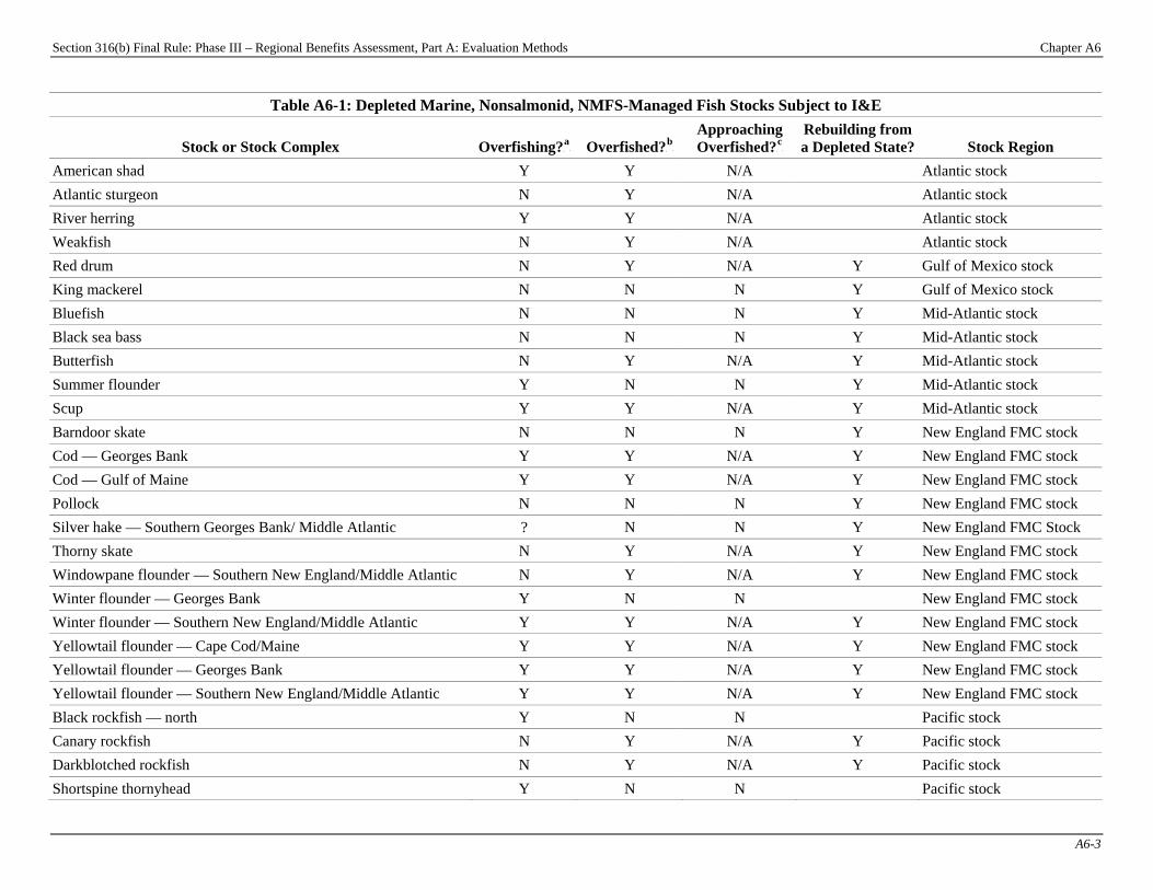
Section 316(b) Final Rule: Phase III – Regional Benefits Assessment, Part A: Evaluation Methods Chapter A6
A6-3
Table A6-1: Depleted Marine, Nonsalmonid, NMFS-Managed Fish Stocks Subject to I&E
Stock or Stock Complex Overfishing?P
aP Overfished?P
bP
Approaching Overfished?P
cP
Rebuilding from a Depleted State? Stock Region
American shad Y Y N/A Atlantic stock Atlantic sturgeon N Y N/A Atlantic stock River herring Y Y N/A Atlantic stock Weakfish N Y N/A Atlantic stock Red drum N Y N/A Y Gulf of Mexico stock King mackerel N N N Y Gulf of Mexico stock Bluefish N N N Y Mid-Atlantic stock Black sea bass N N N Y Mid-Atlantic stock Butterfish N Y N/A Y Mid-Atlantic stock Summer flounder Y N N Y Mid-Atlantic stock Scup Y Y N/A Y Mid-Atlantic stock Barndoor skate N N N Y New England FMC stock Cod — Georges Bank Y Y N/A Y New England FMC stock Cod — Gulf of Maine Y Y N/A Y New England FMC stock Pollock N N N Y New England FMC stock Silver hake — Southern Georges Bank/ Middle Atlantic ? N N Y New England FMC Stock Thorny skate N Y N/A Y New England FMC stock Windowpane flounder — Southern New England/Middle Atlantic N Y N/A Y New England FMC stock Winter flounder — Georges Bank Y N N New England FMC stock Winter flounder — Southern New England/Middle Atlantic Y Y N/A Y New England FMC stock Yellowtail flounder — Cape Cod/Maine Y Y N/A Y New England FMC stock Yellowtail flounder — Georges Bank Y Y N/A Y New England FMC stock Yellowtail flounder — Southern New England/Middle Atlantic Y Y N/A Y New England FMC stock Black rockfish — north Y N N Pacific stock Canary rockfish N Y N/A Y Pacific stock Darkblotched rockfish N Y N/A Y Pacific stock Shortspine thornyhead Y N N Pacific stock
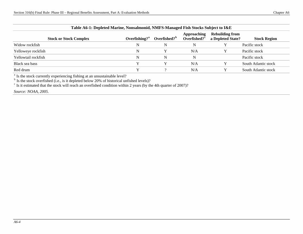
316(b) Final Rule: Phase III – Regional Benefits Assessment, Part A: Evaluation Methods Chapter A6
A6-4
Table A6-1: Depleted Marine, Nonsalmonid, NMFS-Managed Fish Stocks Subject to I&E
Stock or Stock Complex Overfishing?P
aP Overfished?P
bP
Approaching Overfished?P
cP
Rebuilding from a Depleted State? Stock Region
Widow rockfish N N N Y Pacific stock Yelloweye rockfish N Y N/A Y Pacific stock Yellowtail rockfish N N N Pacific stock Black sea bass Y Y N/A Y South Atlantic stock Red drum Y ? N/A Y South Atlantic stock P
aP Is the stock currently experiencing fishing at an unsustainable level?
P
bP Is the stock overfished (i.e., is it depleted below 20% of historical unfished levels)?
P
cP Is it estimated that the stock will reach an overfished condition within 2 years (by the 4th quarter of 2007)?
Source: NOAA, 2005.
Section
Section 316(b) Final Rule: Phase III – Regional Benefits Assessment, Part A: Evaluation Methods Chapter A6
A6-5
A6-1.2 Ecosystem Effects The aquatic resources affected by cooling water intake structures provide a wide range of services. Ecosystem services are the physical, chemical, and biological functions performed by natural resources and the human benefits derived from those functions, including both ecological and human use services (Daily, 1997; Daily et al., 1997). Scientific and public interest in protecting ecosystem services is increasing with the recognition that these services are vulnerable to a wide range of human activities and are difficult, if not impossible, to replace with human technologies (Meffe, 1992). In addition to their importance in providing food and other goods of direct use to humans, the organisms lost to I&E may be critical to the continued functioning of the ecosystems of which they are a part. Fish are essential for energy transfer in aquatic food webs (Summers, 1989), regulation of food web structure, nutrient cycling, maintenance of sediment processes, redistribution of bottom substrates, regulation of carbon fluxes from water to the atmosphere, and maintenance of aquatic biodiversity (Peterson and Lubchenco, 1997; Postel and Carpenter, 1997; Holmlund and Hammer, 1999; Wilson and Carpenter, 1999). Examples of ecological services that may be disrupted by I&E include:
< decreased numbers of ecological keystone, rare, sensitive, or threatened and endangered species; < decreased numbers of popular commercial and recreational fish species that are not fished, perhaps
because the fishery is closed; < increased numbers of exotic or disruptive species that compete well in the absence of species lost to I&E
(I&E may also help remove some exotic or disruptive organisms); < disruption of ecological niches and ecological strategies used by aquatic species; < disruption of energy transfer through the food web; < decreased local biodiversity; < disruption of predator-prey relationships; < disruption of age class structures of species; and < disruption of natural succession processes.
Many of these services can only be maintained by the continued presence of all life stages of fish and other aquatic species in their natural habitats. Reducing I&E losses could contribute to restoring (or preserving) the biological integrity of the ecosystems of substantial national importance. a. Effects on saltwater ecosystems In the 1987 amendments to the CWA, Congress established the National Estuary Program because the “Nation’s estuaries are of great importance to fish and wildlife resources and recreation and economic opportunity. [, and to] maintain the health and ecological integrity of these estuaries is in the national interest” (Water Quality Act, 1987). So far, there are 28 estuaries designated under the National Estuary Program (NEP). In addition, the largest estuary in the United States, Chesapeake Bay, is protected under its own federally mandated program, separate but related to NEP. Table A6-2 shows estuaries from which the sample Phase III facilities draw water. Of the 17 estuaries affected by the surveyed Phase III facilities, 12 are nationally significant estuaries designated under NEP or the Chesapeake Bay Program. Nine, five, and seven of the 17 estuaries affected by the surveyed Phase III facilities have facilities that would also be subject to technology requirements under the “50 MGD for All Waterbodies” option, the “200 MGD for All Waterbodies” option, and the “100 MGD for Certain Waterbodies” option, respectively. Substantial federal and state resources have been directed to NEP to enhance conservation of and knowledge about the estuaries designated under this program. Since 1998, more than $95 million has been devoted to NEP to benefit the health of the nationally significant estuaries (NEP, 2004; U.S. EPA, 2004c). These expenditures reflect high public values for restoring (or protecting) the biological integrity of the ecosystems of substantial national importance.

Section 316(b) Final Rule: Phase III – Regional Benefits Assessment, Part A: Evaluation Methods Chapter A6
A6-6
Table A6-2: Estuaries Affected by Phase III Facilities
Region Estuaries Affected by Potentially
Regulated Phase III FacilitiesP
aP
Designated Under NEP or
the Chesapeake Bay ProgramP
bP
50 MGD All
200 MGD All
100 MGD CWB
Honker Bay (San Francisco Bay) California Kaulakahi Channel San Pablo Bay (San Francisco Bay)
Boston Bay (Massachusetts Bays) Fishers Island Sound (Long Island Sound)
North Atlantic
Penobscot Bay Chesapeake Bay (Chesapeake Bay Program)
Delaware Bay (Delaware Estuary) Fishing Bay (Chesapeake Bay Program) Long Island Sound (Long Island Sound) Newark Bay (New York/New Jersey Harbor)
Mid-Atlantic
Upper Bay (New York/New Jersey Harbor) South Atlantic Savannah River Estuary
Gulf of Mexico Christmas Bay (Galveston Bay)
Galveston Bay (Galveston Bay)
Lavaca Bay Vermilion Bay
P
aP This estimate is based on a total of 314 sample facilities, which represent 629 potentially regulated sample-weighted
facilities. The locations of non-sampled facilities are unknown and could not be included in this analysis. Facilities subject to BPJ requirements are located on these estuaries. P
bP Based on estuaries included in EPA’s National Estuary Program and the Chesapeake Bay Program.
Source: U.S. EPA, 2006b. b. Effects on freshwater ecosystems Reducing I&E at Phase III facilities may also benefit freshwater ecosystems of national significance, including the Great Lakes Basin and Mississippi River. These waterbodies are subject to large-scale ecosystem restoration efforts that are good indicators of great public importance of restoring the ecological health of these ecosystems (Northeast Midwest Institute, 2004; The Upper Mississippi River Basin Association, 2004; U.S. DOI, 2004; USFWS, 2004). The ecosystem restoration efforts focus on many issues, including coastal habitat restoration, protection of fish species, conservation of migratory birds and endangered species. For example, between 1992 and 2001, more than $17 million was devoted to projects to restore and conserve the Great Lakes ecosystem; $102 million was spent on improving the Mississippi River ecosystem (Brescia, 2002; U.S. EPA, 2004b). Reducing I&E of aquatic organisms may improve the quality of aquatic habitat and contribute to improvement of the biological integrity and health of these ecosystems. Finally, reducing I&E in waterbodies that do not have a national significance may contribute to restoration or protection of ecosystems of regional or local importance.
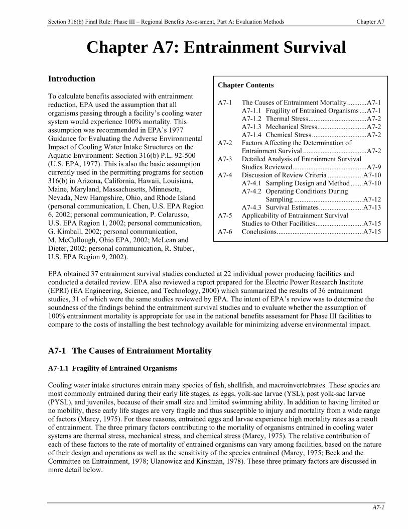
Section 316(b) Final Rule: Phase III – Regional Benefits Assessment, Part A: Evaluation Methods Chapter A7
A7-1
Chapter A7: Entrainment Survival Introduction
Chapter Contents A7-1 The Causes of Entrainment Mortality...........A7-1 A7-1.1 Fragility of Entrained Organisms ....A7-1 A7-1.2 Thermal Stress.................................A7-2 A7-1.3 Mechanical Stress............................A7-2 A7-1.4 Chemical Stress ...............................A7-2 A7-2 Factors Affecting the Determination of Entrainment Survival ....................................A7-2 A7-3 Detailed Analysis of Entrainment Survival Studies Reviewed..........................................A7-9 A7-4 Discussion of Review Criteria ....................A7-10 A7-4.1 Sampling Design and Method .......A7-10 A7-4.2 Operating Conditions During Sampling .......................................A7-12 A7-4.3 Survival Estimates.........................A7-13 A7-5 Applicability of Entrainment Survival Studies to Other Facilities...........................A7-15 A7-6 Conclusions.................................................A7-15
To calculate benefits associated with entrainment reduction, EPA used the assumption that all organisms passing through a facility’s cooling water system would experience 100% mortality. This assumption was recommended in EPA’s 1977 Guidance for Evaluating the Adverse Environmental Impact of Cooling Water Intake Structures on the Aquatic Environment: Section 316(b) P.L. 92-500 (U.S. EPA, 1977). This is also the basic assumption currently used in the permitting programs for section 316(b) in Arizona, California, Hawaii, Louisiana, Maine, Maryland, Massachusetts, Minnesota, Nevada, New Hampshire, Ohio, and Rhode Island (personal communication, I. Chen, U.S. EPA Region 6, 2002; personal communication, P. Colarusso, U.S. EPA Region 1, 2002; personal communication, G. Kimball, 2002; personal communication, M. McCullough, Ohio EPA, 2002; McLean and Dieter, 2002; personal communication, R. Stuber, U.S. EPA Region 9, 2002). EPA obtained 37 entrainment survival studies conducted at 22 individual power producing facilities and conducted a detailed review. EPA also reviewed a report prepared for the Electric Power Research Institute (EPRI) (EA Engineering, Science, and Technology, 2000) which summarized the results of 36 entrainment studies, 31 of which were the same studies reviewed by EPA. The intent of EPA’s review was to determine the soundness of the findings behind the entrainment survival studies and to evaluate whether the assumption of 100% entrainment mortality is appropriate for use in the national benefits assessment for Phase III facilities to compare to the costs of installing the best technology available for minimizing adverse environmental impact. A7-1 The Causes of Entrainment Mortality A7-1.1 Fragility of Entrained Organisms Cooling water intake structures entrain many species of fish, shellfish, and macroinvertebrates. These species are most commonly entrained during their early life stages, as eggs, yolk-sac larvae (YSL), post yolk-sac larvae (PYSL), and juveniles, because of their small size and limited swimming ability. In addition to having limited or no mobility, these early life stages are very fragile and thus susceptible to injury and mortality from a wide range of factors (Marcy, 1975). For these reasons, entrained eggs and larvae experience high mortality rates as a result of entrainment. The three primary factors contributing to the mortality of organisms entrained in cooling water systems are thermal stress, mechanical stress, and chemical stress (Marcy, 1975). The relative contribution of each of these factors to the rate of mortality of entrained organisms can vary among facilities, based on the nature of their design and operations as well as the sensitivity of the species entrained (Marcy, 1975; Beck and the Committee on Entrainment, 1978; Ulanowicz and Kinsman, 1978). These three primary factors are discussed in more detail below.
Section 316(b) Final Rule: Phase III – Regional Benefits Assessment, Part A: Evaluation Methods Chapter A7
A7-2
A7-1.2 Thermal Stress Facilities use cooling water as a means of disposing of waste heat from facility operations. Thus, organisms present in the cooling water are exposed to rapid increases in temperatures above ambient conditions when passing through the cooling water system. This thermal shock causes mortality or sublethal effects that affect further growth and development of entrained eggs and larvae (Schubel et al., 1978; Stauffer, 1980). The magnitude of thermal stress experienced by organisms passing through a facility’s cooling system depends on facility-specific parameters such as intake temperature, maximum temperature, discharge temperature, duration of exposure to elevated temperatures through the facility and in the mixing zone of the discharge canal, the critical thermal maxima of the species, and delta T ()T, i.e., the difference between ambient water temperature and maximum water temperature within the cooling system) (Marcy, 1975; Schubel et al., 1978). The extent of the effect of thermal stress can also vary among the species and life stages of entrained organisms (Schubel et al., 1978; Stauffer, 1980). A7-1.3 Mechanical Stress Entrained organisms are also exposed to significant mechanical stress during passage through a cooling system, which also causes mortality. Types of mechanical stress include effects from turbulence, buffeting, velocity changes, pressure changes, and abrasion from contact with the interior surfaces of the cooling water intake structure (Marcy, 1973; Marcy et al., 1978). The extent of the effect of mechanical stress depends on the design of the facility’s cooling water intake structure and the capacity utilization of operation. Some studies have suggested that mechanical stress may be the dominant cause of entrainment mortality at many facilities (Marcy, 1973; Marcy et al., 1978). For this reason, it has been suggested that the only effective method of minimizing adverse effects to entrained organisms is to reduce the intake of water (Marcy, 1975). A7-1.4 Chemical Stress Chemical biocides are occasionally used within cooling water intake structures to remove biofouling organisms. Chlorine is the active component of the most commonly used biocides (Morgan and Carpenter, 1978; Morgan, 1980). These biocides are used in concentrations sufficient to kill organisms fouling the cooling system structures, and thus cause mortality to the organisms entrained during biocide application. The extent of the effect of chemical stress depends on the concentration of biocide and the timing of its application. Eggs may be less susceptible to biocides than larvae (Lauer et al., 1974; Morgan and Carpenter, 1978). Tolerance to biocides may also vary according to species. However, most species have been shown to be affected at low concentrations, <0.5 ppm, of residual chlorine (Morgan and Carpenter, 1978). A7-2 Factors Affecting the Determination of Entrainment Survival There are many challenges that must be overcome in the design of a sampling program intended to accurately establish the magnitude of entrainment survival (Lauer et al., 1974; Marcy, 1975; Coutant and Bevelhimer, 2001). Samples are almost certain not to be fully representative of the community of organisms experiencing entrainment. Some species are extremely fragile and disintegrate during collection or when preserved, and are thus not documented when samples are processed (Boreman and Goodyear, 1981). This is particularly true for the most fragile life stages, such as eggs and yolk-sac larvae of many species. All sampling devices are selective for a certain size range of organisms, so a number of sampling methods would have to be employed to accurately sample the broad size range of organisms subject to entrainment. The relative ability of different organisms to avoid sampling devices also determines abundance and species composition estimated from samples (Boreman and Goodyear, 1981). This avoidance ability varies with the size, motility, and condition of the organisms. If dead or dying organisms tend to settle out, then sampling will be selective for the live, healthy specimens (Marcy, 1975). If, on the other hand, the healthy, more motile specimens are able to avoid sampling gear, the sampling will tend to be selective for dead or stunned specimens. The patchy distribution of many species (Day et al., 1989; Valiela, 1995) creates difficulties in developing precise estimates of organism densities (Boreman and Goodyear,

Section 316(b) Final Rule: Phase III – Regional Benefits Assessment, Part A: Evaluation Methods Chapter A7
A7-3
1981). The patchier the distribution, the greater the number of samples required to reduce the uncertainty associated with the density estimates to an acceptable level. The factors just discussed affect the ability to accurately establish the type and abundance of organisms present at the intake and discharge of a cooling water system. A second suite of factors, superimposed on the first, affects the ability to estimate the percentages of those organisms that are alive and dead at those two locations. The greatest challenge to be overcome is posed by the fragility of the organisms being studied. The early life stages of most species are so fragile that they may experience substantial mortality simply due to being sampled, both from contact with the sampling gear and in being handled for subsequent evaluation. For example, Marcy (1973) reported on the effects of current velocity on percent mortality of ichthyoplankton taken in plankton nets, and found sampling mortality of 18% at velocities of 0.3 to 0.6 m/sec. The loss or damage of organisms beyond identification during plant passage causes overestimations of the true fraction of live organisms in the discharge samples, because the disintegrated organisms are extruded from the sampling device (Boreman and Goodyear, 1981). The entrainment survival studies addressed in this review quantified survival by estimating the percentage of organisms categorized as alive, stunned, or dead present in samples collected at the intake and discharge locations of a facility. In the studies reviewed, a variety of methods were used to determine the physiological state of sampled organisms, ranging from placing the sampled organisms in various types of holding containers for observation to the use of devices specifically designed for assessment of larval survival, such as a larval table. A variety of criteria was also used in these studies to categorize the physiological status of the organisms, such as opacity as an indicator of a dead egg, and movement of a larva in response to being touched as an indicator of being alive or stunned. The lack of standardized procedures applied for assessing physiological condition in all of the studies reviewed made comparisons of the study findings difficult. When quantifying entrainment survival, these studies used the estimates of the percentage dead from samples collected at the intake as controls to correct the samples at the discharge for mortality associated with natural causes and with sampling and handling stress. The use of intake samples as controls requires the assumption that sampling- and handling-induced mortality rates be the same at the intake and discharge, which, in turn, requires that sampling methods and conditions be nearly identical in both locations (Marcy, 1973). This requirement is difficult to meet at most facilities because of the differences in the physical structures and hydrodynamic conditions at intakes and discharges (e.g., frequently high velocity, turbulent flow at discharges versus lower velocity, laminar flows at intakes). In many cases, the location and design of the cooling water intake and discharge structures may preclude use of the same type of sampling gear in both locations. Another assumption implicit in this approach is that mortality due to entrainment is entirely independent of mortality due to sampling and handling and that there is no interaction between these stresses, an assumption that is acknowledged but never proven in the studies reviewed. The percent alive in the intake control is frequently well below 100% because these fragile organisms experience substantial mortality from stresses caused by being collected. An additional factor contributing to the less than 100% alive in intake samples is that some dead organisms may be present in the water column being sampled because of natural mortality or recirculation of water discharged from the cooling system. In many studies, the survival in the intake sample is extremely low; for example, the intake survival for bay anchovy was 0% in studies conducted at Bowline (Ecological Analysts, 1978a), Brayton Point (Lawler, Matusky & Skelly Engineers, 1999), and Indian Point (Ecological Analysts, 1978c; EA Engineering, Science, and Technology, 1989). The studies reviewed corrected their discharge survival estimates to account for the control sample mortality by using the percent alive in the intake control samples in the following manner. First, the proportion initially alive at the intake (PBIB) and discharge (PBDB) samples was determined, for each species in most cases, using the following equation:
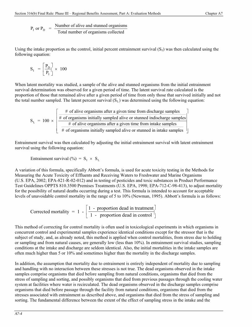
Section 316(b) Final Rule: Phase III – Regional Benefits Assessment, Part A: Evaluation Methods Chapter A7
A7-4
P or P = Number of alive and stunned organismsTotal number of organisms collected
I D
Using the intake proportion as the control, initial percent entrainment survival (SBIB) was then calculated using the following equation:
S = PP
100 ID
I
⎡
⎣⎢
⎤
⎦⎥ ×
When latent mortality was studied, a sample of the alive and stunned organisms from the initial entrainment survival determination was observed for a given period of time. The latent survival rate calculated is the proportion of those that remained alive after a given period of time from only those that survived initially and not the total number sampled. The latent percent survival (SBLB) was determined using the following equation:
S = 100
# of alive organisms after a given time from discharge samples# of organisms initially sampled alive or stunned indischarge samples
# of alive organisms after a given time from intake samples# of organisms initially sampled alive or stunned in intake samples
L ×
⎡
⎣
⎢⎢⎢⎢
⎤
⎦
⎥⎥⎥⎥
Entrainment survival was then calculated by adjusting the initial entrainment survival with latent entrainment survival using the following equation:
Entrainment survival (%) = S SI L× A variation of this formula, specifically Abbott’s formula, is used for acute toxicity testing in the Methods for Measuring the Acute Toxicity of Effluents and Receiving Waters to Freshwater and Marine Organisms (U.S. EPA, 2002; EPA-821-R-02-012) and in testing of pesticides and toxic substances in Product Performance Test Guidelines OPPTS 810.3500 Premises Treatments (U.S. EPA, 1998; EPA-712-C-98-413), to adjust mortality for the possibility of natural deaths occurring during a test. This formula is intended to account for acceptable levels of unavoidable control mortality in the range of 5 to 10% (Newman, 1995). Abbott’s formula is as follows:
Corrected mortality = 1 - 1 - proportion dead in treatment1 - proportion dead in control
⎡
⎣⎢
⎤
⎦⎥
This method of correcting for control mortality is often used in toxicological experiments in which organisms in concurrent control and experimental samples experience identical conditions except for the stressor that is the subject of study, and, as already noted, this method is applied when control mortalities, from stress due to holding or sampling and from natural causes, are generally low (less than 10%). In entrainment survival studies, sampling conditions at the intake and discharge are seldom identical. Also, the initial mortalities in the intake samples are often much higher than 5 or 10% and sometimes higher than the mortality in the discharge samples. In addition, the assumption that mortality due to entrainment is entirely independent of mortality due to sampling and handling with no interaction between these stresses is not true. The dead organisms observed in the intake samples comprise organisms that died before sampling from natural conditions, organisms that died from the stress of sampling and sorting, and possibly organisms that died from previous passages through the cooling water system at facilities where water is recirculated. The dead organisms observed in the discharge samples comprise organisms that died before passage through the facility from natural conditions, organisms that died from the stresses associated with entrainment as described above, and organisms that died from the stress of sampling and sorting. The fundamental difference between the extent of the effect of sampling stress in the intake and the
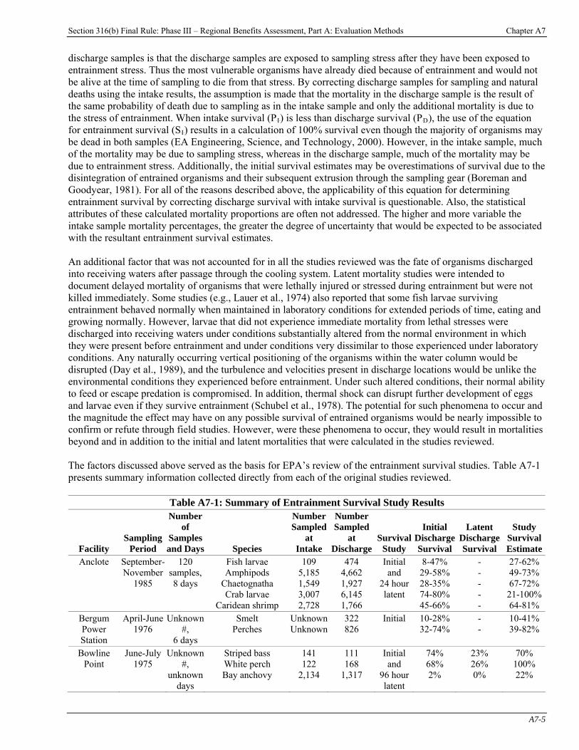
Section 316(b) Final Rule: Phase III – Regional Benefits Assessment, Part A: Evaluation Methods Chapter A7
A7-5
discharge samples is that the discharge samples are exposed to sampling stress after they have been exposed to entrainment stress. Thus the most vulnerable organisms have already died because of entrainment and would not be alive at the time of sampling to die from that stress. By correcting discharge samples for sampling and natural deaths using the intake results, the assumption is made that the mortality in the discharge sample is the result of the same probability of death due to sampling as in the intake sample and only the additional mortality is due to the stress of entrainment. When intake survival (PBIB) is less than discharge survival (PBDB), the use of the equation for entrainment survival (SBIB) results in a calculation of 100% survival even though the majority of organisms may be dead in both samples (EA Engineering, Science, and Technology, 2000). However, in the intake sample, much of the mortality may be due to sampling stress, whereas in the discharge sample, much of the mortality may be due to entrainment stress. Additionally, the initial survival estimates may be overestimations of survival due to the disintegration of entrained organisms and their subsequent extrusion through the sampling gear (Boreman and Goodyear, 1981). For all of the reasons described above, the applicability of this equation for determining entrainment survival by correcting discharge survival with intake survival is questionable. Also, the statistical attributes of these calculated mortality proportions are often not addressed. The higher and more variable the intake sample mortality percentages, the greater the degree of uncertainty that would be expected to be associated with the resultant entrainment survival estimates. An additional factor that was not accounted for in all the studies reviewed was the fate of organisms discharged into receiving waters after passage through the cooling system. Latent mortality studies were intended to document delayed mortality of organisms that were lethally injured or stressed during entrainment but were not killed immediately. Some studies (e.g., Lauer et al., 1974) also reported that some fish larvae surviving entrainment behaved normally when maintained in laboratory conditions for extended periods of time, eating and growing normally. However, larvae that did not experience immediate mortality from lethal stresses were discharged into receiving waters under conditions substantially altered from the normal environment in which they were present before entrainment and under conditions very dissimilar to those experienced under laboratory conditions. Any naturally occurring vertical positioning of the organisms within the water column would be disrupted (Day et al., 1989), and the turbulence and velocities present in discharge locations would be unlike the environmental conditions they experienced before entrainment. Under such altered conditions, their normal ability to feed or escape predation is compromised. In addition, thermal shock can disrupt further development of eggs and larvae even if they survive entrainment (Schubel et al., 1978). The potential for such phenomena to occur and the magnitude the effect may have on any possible survival of entrained organisms would be nearly impossible to confirm or refute through field studies. However, were these phenomena to occur, they would result in mortalities beyond and in addition to the initial and latent mortalities that were calculated in the studies reviewed. The factors discussed above served as the basis for EPA’s review of the entrainment survival studies. Table A7-1 presents summary information collected directly from each of the original studies reviewed.
Table A7-1: Summary of Entrainment Survival Study Results
Facility Sampling
Period
Number of
Samples and Days Species
Number Sampled
at Intake
Number Sampled
at Discharge
Survival Study
Initial Discharge Survival
Latent DischargeSurvival
Study Survival Estimate
Anclote September-November
1985
120 samples, 8 days
Fish larvae Amphipods
Chaetognatha Crab larvae
Caridean shrimp
109 5,185 1,549 3,007 2,728
474 4,662 1,927 6,145 1,766
Initial and
24 hour latent
8-47% 29-58% 28-35% 74-80% 45-66%
- - - - -
27-62%49-73%67-72%21-100%64-81%
Bergum Power Station
April-June 1976
Unknown #,
6 days
Smelt Perches
UnknownUnknown
322 826
Initial 10-28% 32-74%
- -
10-41%39-82%
Bowline Point
June-July 1975
Unknown #,
unknown days
Striped bass White perch Bay anchovy
141 122
2,134
111 168
1,317
Initial and
96 hour latent
74% 68% 2%
23% 26% 0%
70% 100% 22%
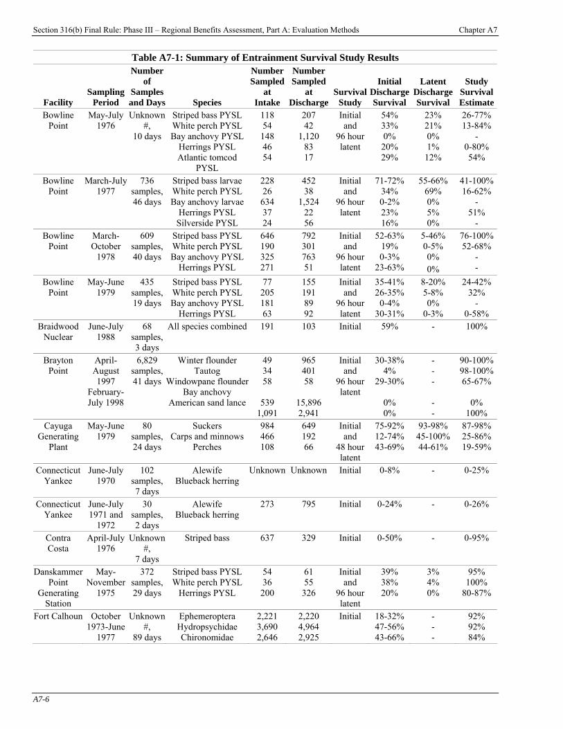
Section 316(b) Final Rule: Phase III – Regional Benefits Assessment, Part A: Evaluation Methods Chapter A7
A7-6
Table A7-1: Summary of Entrainment Survival Study Results
Facility Sampling
Period
Number of
Samples and Days Species
Number Sampled
at Intake
Number Sampled
at Discharge
Survival Study
Initial Discharge Survival
Latent DischargeSurvival
Study Survival Estimate
Bowline Point
May-July 1976
Unknown #,
10 days
Striped bass PYSLWhite perch PYSLBay anchovy PYSL
Herrings PYSL Atlantic tomcod
PYSL
118 54 148 46 54
207 42
1,120 83 17
Initial and
96 hour latent
54% 33% 0% 20% 29%
23% 21% 0% 1%
12%
26-77%13-84%
- 0-80% 54%
Bowline Point
March-July 1977
736 samples, 46 days
Striped bass larvaeWhite perch PYSLBay anchovy larvae
Herrings PYSL Silverside PYSL
228 26 634 37 24
452 38
1,524 22 56
Initial and
96 hour latent
71-72% 34% 0-2% 23% 16%
55-66% 69% 0% 5% 0%
41-100%16-62%
- 51%
- Bowline
Point March-October
1978
609 samples, 40 days
Striped bass PYSLWhite perch PYSLBay anchovy PYSL
Herrings PYSL
646 190 325 271
792 301 763 51
Initial and
96 hour latent
52-63% 19% 0-3%
23-63%
5-46% 0-5% 0% 0%
76-100%52-68%
- -
Bowline Point
May-June 1979
435 samples, 19 days
Striped bass PYSLWhite perch PYSLBay anchovy PYSL
Herrings PYSL
77 205 181 63
155 191 89 92
Initial and
96 hour latent
35-41% 26-35%
0-4% 30-31%
8-20% 5-8% 0%
0-3%
24-42%32%
- 0-58%
Braidwood Nuclear
June-July 1988
68 samples, 3 days
All species combined 191 103 Initial 59% - 100%
Brayton Point
April-August 1997
February-July 1998
6,829 samples, 41 days
Winter flounder Tautog
Windowpane flounder Bay anchovy
American sand lance
49 34 58
539
1,091
965 401 58
15,896 2,941
Initial and
96 hour latent
30-38% 4%
29-30%
0% 0%
- - - - -
90-100%98-100%65-67%
0%
100% Cayuga
Generating Plant
May-June 1979
80 samples, 24 days
Suckers Carps and minnows
Perches
984 466 108
649 192 66
Initial and
48 hour latent
75-92% 12-74% 43-69%
93-98% 45-100% 44-61%
87-98%25-86%19-59%
Connecticut Yankee
June-July 1970
102 samples, 7 days
Alewife Blueback herring
Unknown Unknown Initial 0-8% - 0-25%
Connecticut Yankee
June-July 1971 and
1972
30 samples, 2 days
Alewife Blueback herring
273 795 Initial 0-24% - 0-26%
Contra Costa
April-July 1976
Unknown #,
7 days
Striped bass 637 329 Initial 0-50% - 0-95%
Danskammer Point
Generating Station
May-November
1975
372 samples, 29 days
Striped bass PYSLWhite perch PYSL
Herrings PYSL
54 36 200
61 55 326
Initial and
96 hour latent
39% 38% 20%
3% 4% 0%
95% 100%
80-87%
Fort Calhoun October 1973-June
1977
Unknown #,
89 days
Ephemeroptera Hydropsychidae Chironomidae
2,221 3,690 2,646
2,220 4,964 2,925
Initial 18-32% 47-56% 43-66%
- - -
92% 92% 84%
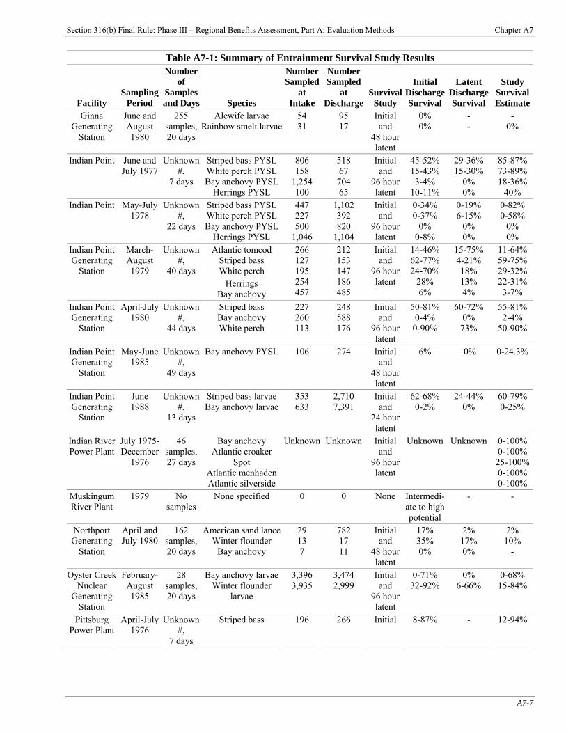
Section 316(b) Final Rule: Phase III – Regional Benefits Assessment, Part A: Evaluation Methods Chapter A7
A7-7
Table A7-1: Summary of Entrainment Survival Study Results
Facility Sampling
Period
Number of
Samples and Days Species
Number Sampled
at Intake
Number Sampled
at Discharge
Survival Study
Initial Discharge Survival
Latent DischargeSurvival
Study Survival Estimate
Ginna Generating
Station
June and August 1980
255 samples, 20 days
Alewife larvae Rainbow smelt larvae
54 31
95 17
Initial and
48 hour latent
0% 0%
- -
- 0%
Indian Point June and July 1977
Unknown #,
7 days
Striped bass PYSLWhite perch PYSLBay anchovy PYSL
Herrings PYSL
806 158
1,254 100
518 67 704 65
Initial and
96 hour latent
45-52% 15-43%
3-4% 10-11%
29-36%15-30%
0% 0%
85-87%73-89%18-36%
40% Indian Point May-July
1978 Unknown
#, 22 days
Striped bass PYSLWhite perch PYSLBay anchovy PYSL
Herrings PYSL
447 227 500
1,046
1,102 392 820
1,104
Initial and
96 hour latent
0-34% 0-37%
0% 0-8%
0-19% 6-15%
0% 0%
0-82% 0-58%
0% 0%
Indian Point Generating
Station
March-August 1979
Unknown #,
40 days
Atlantic tomcod Striped bass White perch
Herrings Bay anchovy
266 127 195 254 457
212 153 147 186 485
Initial and
96 hour latent
14-46% 62-77% 24-70%
28% 6%
15-75%4-21% 18% 13% 4%
11-64%59-75%29-32%22-31%
3-7% Indian Point Generating
Station
April-July 1980
Unknown #,
44 days
Striped bass Bay anchovy White perch
227 260 113
248 588 176
Initial and
96 hour latent
50-81% 0-4%
0-90%
60-72%0%
73%
55-81%2-4%
50-90%
Indian Point Generating
Station
May-June 1985
Unknown #,
49 days
Bay anchovy PYSL 106 274 Initial and
48 hour latent
6% 0% 0-24.3%
Indian Point Generating
Station
June 1988
Unknown #,
13 days
Striped bass larvaeBay anchovy larvae
353 633
2,710 7,391
Initial and
24 hour latent
62-68% 0-2%
24-44%0%
60-79%0-25%
Indian River Power Plant
July 1975-December
1976
46 samples, 27 days
Bay anchovy Atlantic croaker
Spot Atlantic menhadenAtlantic silverside
Unknown Unknown Initial and
96 hour latent
Unknown Unknown 0-100%0-100%25-100%0-100%0-100%
Muskingum River Plant
1979 No samples
None specified 0 0 None Intermedi-ate to high potential
- -
Northport Generating
Station
April and July 1980
162 samples, 20 days
American sand lanceWinter flounder
Bay anchovy
29 13 7
782 17 11
Initial and
48 hour latent
17% 35% 0%
2% 17% 0%
2% 10%
-
Oyster Creek Nuclear
Generating Station
February-August 1985
28 samples, 20 days
Bay anchovy larvaeWinter flounder
larvae
3,396 3,935
3,474 2,999
Initial and
96 hour latent
0-71% 32-92%
0% 6-66%
0-68% 15-84%
Pittsburg Power Plant
April-July 1976
Unknown #,
7 days
Striped bass 196 266 Initial 8-87% - 12-94%

Section 316(b) Final Rule: Phase III – Regional Benefits Assessment, Part A: Evaluation Methods Chapter A7
A7-8
Table A7-1: Summary of Entrainment Survival Study Results
Facility Sampling
Period
Number of
Samples and Days Species
Number Sampled
at Intake
Number Sampled
at Discharge
Survival Study
Initial Discharge Survival
Latent DischargeSurvival
Study Survival Estimate
Port Jefferson
April 1978
94 samples, 5 days
Winter flounder Sand lance
Fourbeard rocklingAmerican eel
Sculpin
36 249 216 107 22
26 191 144 96 17
Initial and
96 hour latent
0-23% 12-40% 19-21% 94-96%
88%
50% 0-10%
- 71-96%
-
65% 25-86%73-100%
100% 75%
PG&E Potrero
January 1979
25 samples
Pacific herring 546 716 Initial and
96 hour latent
16% - 70%
Quad Cities Nuclear Station
June 1978
Unknown #,
5 days
Freshwater drum Minnows
378 278
916 307
Initial and
24 hour latent
0-71% 2-75%
- -
2-62% 7-63%
Quad Cities Nuclear Station
April-June 1984
Unknown #,
8 days
Freshwater drum Carp
Buffalo
UnknownUnknownUnknown
UnknownUnknownUnknown
Initial and
24 hour latent
Unknown Unknown Unknown
- - -
63% 92-97%
94%
Roseton Generating
Station
May-November
1975
672 samples, 41 days
Striped bass PYSLWhite perch PYSL
Herrings PYSL
100 77 471
172 97 833
Initial and
96 hour latent
62% 29% 26%
6% 1% 0%
38% - -
Roseton Generating
Station
June-July 1976
Unknown #,
27 days
Striped bass PYSLWhite perch PYSL
Herring PYSL
93 401
1,054
80 349 645
Initial and
96 hour latent
14-43% 6-42% 5-29%
- -
0%
19-58%11-79%10-59%
Roseton Generating
Station
March May-July
1977
Unknown #,
unknown days
Striped bass PYSLWhite perch PYSL
Herring PYSL Atlantic tomcod YSL
427 251 880
1,178
765 266
1,344 1,345
Initial and
96 hour latent
3-29% 0-17% 0-5% 16%
18% 27% 0%
40%
6-58% 0-52% 0-19% 41%
Roseton Generating
Station
March July-July
1978
256 samples, 30 days
Striped bass PYSLWhite perch PYSL
Herring PYSL Atlantic tomcod
PYSL
123 395
1,274 83
211 459
1,089 153
Initial and
96 hour latent
27-50% 0-35% 0-10%
33-45%
18% 10% 0%
36%
46% 56-96%
0% 39%
Roseton Generating
Station
May-July 1980
1,431 samples, 42 days
Striped bass PYSLWhite perch PYSL
Herring PYSL
245 194 812
425 366
1,252
Initial and
48 hour latent
46-61% 30-59% 7-31%
48-56% 27-62% 1-3%
88% 67% 23%
Salem Generating
Station
1977-1982 640 samples, 38 days
Spot Herrings
Atlantic croaker Striped bass White perch Bay anchovy
Weakfish
66 8 - - - - -
130 14 - - - - -
Onsite and
simulated studies
74.1% 7.1%
- - - - -
- 0% - - - - -
0-76% 2-74% 0-60%
32-46%30-70%
2-3% 14-56%

Section 316(b) Final Rule: Phase III – Regional Benefits Assessment, Part A: Evaluation Methods Chapter A7
A7-9
A review of the data in Table A7-1 shows that the majority of the studies were conducted at facilities located in a limited geographical region of the country: 24 of the studies were conducted in the northeastern region of the United States. This may explain why these studies provide entrainment survival estimates for relatively few, only 24, species or families of fish. The majority of survival estimates in these studies were for striped bass, white perch, bay anchovy, and herrings. Also, the majority of these studies are over 20 years old, with 25 of the studies conducted in the 1970s. Thus, the results on species composition and abundance are not necessarily indicative of current conditions, with improved water quality due to the enactment of the Clean Water Act in 1972. Entrainment survival in these studies was also estimated with relatively short sampling periods, with the 15 studies using sampling periods of approximately two months long. Also, the sampling periods did not always correspond to peak egg and larval abundance in the waterbody. Twelve of these studies determined that sample sizes of fewer than 100 individuals for a particular species at the discharge station were sufficient to give an accurate estimation of entrainment survival. These small sample sizes are not be sufficient to provide accurate estimates of entrainment survival given that these facilities entrain organisms on the order of millions to billions per year. Also, small sample sizes in conjunction with the high variability of entrainment survival increase the uncertainty associated with these estimations. The small sample sizes allowed for limited study of latent survival, and no facility attempted to study latent physiological effects of entrainment on a species, such as the possible effects on growth rates, maturation, fertility, and vulnerability to natural mortality. The nature of the equation for entrainment survival results in estimates substantially higher than the proportion of survival in the discharge samples because of its use of a correction for mortality in the intake samples, which is often quite high. The fact that the existing studies are characterized by high uncertainty, high variability, and the potential for high bias (Boreman and Goodyear, 1981) complicates efforts to synthesize the various results in a manner that would provide useful generalizations of the results or application to other particular facilities. For these reasons, EPA believes that the reported results do not provide a clear indication as to the extent of entrainment survival significantly above 0% to be used as a defensible assumption to calculate benefits for the section 316(b) rulemaking. A7-3 Detailed Analysis of Entrainment Survival Studies Reviewed The summary tables at the end of this chapter provide detailed summary descriptions of each of the 37 studies reviewed. EPA reviewed these studies to determine if they were conducted in a manner that provides adequate representation of the current probability of entrainment survival at the facility. The criteria EPA used to evaluate the studies focused on three main themes: the sampling effort of the study, the operating conditions of the facility during the study, and the survival estimates determined as the result of the study. Specifically, EPA asked the following questions: Sampling:
< When were samples collected? < With what frequency were samples collected? < Were samples collected when organisms were spawning, or at peak abundance? < What time of day were samples collected? < What was the number of replicates per sampling date? < Were the intake and discharge samples collected at the same time so the results can be compared? < How long was each sample collected? < What method was used to collect samples? < At what depth were samples collected? < What was the location of the samples collected at the intake and discharge? < Which water quality parameters were measured? < Were dissolved organic carbon (DOC) and particulate organic carbon (POC) measured? < What was the velocity at the intake and at the discharge?
Section 316(b) Final Rule: Phase III – Regional Benefits Assessment, Part A: Evaluation Methods Chapter A7
A7-10
Operating conditions during sampling:
< How many generating units at the facility were in operation? < How many pumps at the facility were in operation? < What was the intake temperature range, the discharge temperature range, and the )T range to which
organisms were exposed? < Were biocides in use?
Survival estimation:
< How many sampling events occurred? < What was the total number of samples collected? < What was the total number of organisms collected? < How many organisms are entrained each year at this facility? < Did the study take into account fragmented organisms? < Were the number of organisms collected at the intake and at the discharge comparable? < What were the most abundant species collected? < Were stunned larvae included with live larvae in survival estimates? < Did the facility omit dead and opaque organisms from the count of dead organisms? < How was latent survival studied? < Were data sampled from all times and operating conditions combined to determine entrainment survival? < What were the controls for the study? < What was the range of intake survival determined by the study? < What was the range of discharge survival determined by the study? < How was entrainment survival calculated? < Were confidence intervals or standard errors calculated? < Were significant differences tested between intake and discharge survival? < Was entrainment survival calculated for species with low sample sizes, such as fewer than 100
organisms? < Was egg survival studied? < Was there any trend evident in larval survival? < Were the raw data provided to verify results? < What was the trend of survival with regard to temperature? < What was the extent of mechanical mortality? < What quality control procedures were used? < Was the study peer reviewed?
A7-4 Discussion of Review Criteria In this section, the criteria EPA used to review the entrainment survival studies are discussed in depth to give a better indication of the soundness of the science behind a facility’s estimate of potential survival. A7-4.1 Sampling Design and Method These aspects of the sampling effort are relevant to whether the samples collected are representative of all organisms experiencing entrainment with regard to taxa and size classes, whether the estimates of densities and numbers are accurate and precise, and whether the survival estimates for the intake and discharge can be validly compared (Marcy, 1975; Boreman and Goodyear, 1981). Sampling should be carefully planned to minimize any potential bias (Marcy, 1975; Boreman and Goodyear, 1981). Studies should be conducted throughout the parts of the year when substantial numbers of organisms are entrained. Any possible survival may vary with factors that change seasonally, such as organism size and life stage and ambient water temperature. Most studies attempted to collect samples during times of peak abundance, although the sampling frequency may not have been sufficient to
Section 316(b) Final Rule: Phase III – Regional Benefits Assessment, Part A: Evaluation Methods Chapter A7
A7-11
fully capture peak densities. Of those reviewed by EPA, six studies did not correspond with the timing of peak densities at that location. Even if a study is limited to the early life stages of particular fish or shellfish, survival differences among sizes and life stages and seasonal or temperature-related changes in entrainment survival must be quantified. The timing of the sample collection for an entrainment survival study can influence results in a number of ways, such that results from studies collected during one period may not be representative of potential effects during other periods. For instance, samples collected when the intake temperatures are low or late in a spawning season when larvae are larger can produce estimates of entrainment survival that may be higher than at other times. Thus, studies need to be conducted throughout the entire spawning season to accurately characterize overall entrainment mortality if entrainment survival is found to vary with life stage or size of each species entrained. For the same reason, it may not be appropriate to develop average survival estimates from samples collected under different environmental conditions (in particular under different temperature regimes) and from only parts of a spawning period for a particular species. This was done in almost all the studies reviewed by EPA, which causes their results to be of questionable value. This also makes it difficult for EPA to synthesize the results of these studies into a meaningful average value of entrainment survival to be used in a national benefits assessment. Many studies collected samples at night to ensure high numbers of organisms in their samples because larvae rise to the surface at night to feed and avoid predation (Marcy, 1975; Day et al., 1989). This practice will bias results because the samples will contain a disproportionate number of live organisms than that which is actually present in the water column. There is evidence that dead organisms will sink to the bottom of the water column after entrainment (Marcy, 1975). Twenty-four studies indicated that most sampling took place at night. For many studies, the depth of sampling is not noted and thus it is unclear whether the samples were collected near the surface, at mid-depth, or near the bottom of the water column. Any potential for bias due to a higher percentage of alive organisms present near the surface could not be assessed. The method of sampling should be selected to cause the least amount of mortality possible and the mesh size should be fine enough to capture disintegrated or fragmented organisms. Many studies sampled organisms using sampling instruments with mesh size greater than or equal to 500 :m. This may not be fine enough to capture disintegrated or fragmented organisms in the discharge. Attention should be given to the mesh size of sampling instruments to be sure that the targeted sample is not extruded through the mesh. Intake and discharge sampling should be paired to be sure that the same population of organisms is sampled and subsequently compared. In 12 studies examined, it is unknown if the samples at the intake and discharge were paired. In some studies, samples were not collected at all locations during all sampling events. In other studies, twice as many samples were collected at the discharge than at the intake. Also, in many instances, the intake samples were collected at different generating units of the facility than the discharge samples. Average elapsed times for sample collection were given, and it is unclear if the same elapsed time was used at both locations to give an accurate depiction of organismal densities. The time elapsed during sample collection or the volume of water sampled should be identical in the paired intake and discharge samples to ensure valid comparisons of samples. It was not indicated in any of the studies reviewed whether the same volume of water was sampled in all the intake and discharge samples. If intake samples are to be compared to discharge samples, consistent sampling methods must be used at the two locations so that the samples contain the same density of organisms. The location of the intake sampling is important because it may contain organisms that already died because of the changes in velocity near the intake. Two studies reviewed collected intake samples after the water had entered the cooling system. The location of the discharge sampling is also important. Samples collected from the end of the discharge canal may not contain organisms that died from passage through the facility because of the tendency of dead organisms to settle out of the water column in the discharge canal. Samples collected from the discharge pipe may not contain organisms that died from thermal effects of entrainment because the samples are collected before the full effects of thermal exposure were experienced. Fourteen studies reviewed collected discharge samples from the discharge pipe. It is also unknown if the samples collected in the discharge canal or from the receiving water contained organisms in the dilution water that bypassed the cooling water system. Five studies
Section 316(b) Final Rule: Phase III – Regional Benefits Assessment, Part A: Evaluation Methods Chapter A7
A7-12
reviewed collected discharge samples in the receiving water downstream from the discharge canal, which can result in samples containing organisms that never passed through the cooling water system. The velocity at the intake and discharge should also be recorded to determine the potential to cause mortality. Fourteen of the studies noted the velocity at the intake, at the discharge, or both. For the ones that did not give both intake and discharge velocities, it is unknown whether the velocities at the two sampling sites were comparable, and thus whether the mortalities due to velocity-related sampling stress were comparable at the two locations. Water chemistry conditions also need to be recorded to be sure conditions are similar at all sampling locations. Water quality parameters include measurements of dissolved oxygen, pH, and conductivity in the through-plant water, at the discharge point, and in the containers or impoundments in which the entrained organism are kept when determining latent mortality. Eighteen studies reviewed gave some indication that water quality parameters were measured. However, it is unclear whether measurements were collected at both the intake and the discharge, and only one study reviewed indicated that water quality parameters were measured in latent mortality studies (EA Engineering, Science, and Technology, 1986). A7-4.2 Operating Conditions During Sampling Mortality due to entrainment stress is affected by the operating characteristics of the power facility. The conditions under which the samples are collected are extremely important and, therefore, the results can be assumed to represent possible survival only when the facility is operating under those same conditions and at that time of year, and may not represent any potential for survival at all times. For example, results of studies conducted when the plant was not generating power (and thus not transferring heat to the cooling water) would not be applicable to impacts when it was in full operation. The magnitude of mechanical stress is dependent on the design of the facility’s cooling water intake structure. The physical and operating conditions of the facility must be recorded to determine the effect on entrainment survival. The percentage of the maximum load at which the facility is operating must be recorded at the time of sampling to indicate the extent to which organisms are exposed to stress. The number of generating units was highly variable or unknown in many of the studies reviewed. Only one study indicated that the facility operated at peak load to maximize temperature stress during the time of sampling. Eight studies indicated that power was generated during only a portion of time in the sampling period. To fully account for the effects of mechanical stressors on entrainment survival, the study must reflect the speed and pressure changes within the condenser, the number of pumps in operation, the occurrence of abrasive surfaces, and the turbulence within the condenser. In addition, it is important to note the number and arrangement of generating units, parallel or in sequence, which may expose organisms to entrainment in multiple structures. Survival should be studied under the range of facility conditions that may influence survival, for example, intake flow or capacity utilization and ambient (intake) water temperature and )T. The effect of temperature can be species-specific since different fishes have different critical thermal maxima. The maximum temperature to which organisms may be exposed while passing through the facility may cause instant death in some species but not others. To assess the effect of thermal stressors on entrainment survival, the study must determine the temperature regime of the facility. Specifically, the study must record the temperature at both the intake and the discharge point for each component of the facilities system: temperature changes within the system, including the inflow temperature; maximum temperature; )T; rate of temperature change; and the temperature of the water to which the organisms are discharged. It is also important to measure the duration of time an organism is entrained and thus exposed to the thermal conditions within the condenser and in the mixing zone of the discharge canal. This information was not provided in the studies reviewed by EPA. Also, in those studies that attempted to relate survival to temperature stress, too few samples were collected at different temperature ranges to give an adequate representation of survival in that range. The EPRI report sorted larval entrainment survival data by discharge temperature and concluded that survivability decreased as the discharge temperature increased (EA Engineering, Science, and Technology, 2000). The lowest probability of larval survival occurred at temperatures greater than 33 °C. In the studies reviewed by EPA, a noticeable decline in survival estimates occurred at discharge temperatures above 30 °C. The amount of time that a facility discharges water in different temperature ranges and survival estimates at that temperature range should be weighted when
Section 316(b) Final Rule: Phase III – Regional Benefits Assessment, Part A: Evaluation Methods Chapter A7
A7-13
attempting to determine the survival estimate throughout the year, rather than using an average survival during the sampling period, which may not adequately reflect operating conditions throughout the year. To properly account for chemical stressors, the timing, frequency, methods, concentrations, and duration of biocide use for the control of biofouling must be determined. The extent to which biocides are routinely used is unknown. The studies reviewed by EPA were all conducted at times when biocides were not in use because the biocide use would be expected to kill all organisms. Thus, the results of these studies do not account for biocide impacts and only reflect other times when biocides are not in use at the particular facility. A reduced survival estimate for the proportion of time when biocides were in use would have to be incorporated into any estimation of annual mean entrainment mortality value for a facility for that estimate to be valid. A7-4.3 Survival Estimates Many of the entrainment survival studies reviewed did not account for the extent to which the fragile life stages are fragmented and disintegrated by both sampling and entrainment. Only six of the studies acknowledged that the entrainment survival estimates were indicative only of alive and stunned identifiable organisms out of all those sampled and enumerated that were at least 50% intact. In such circumstances, an important proportion of entrained dead (fragmented) organisms is omitted from the calculated estimate of survival. Entrainment survival studies should not limit their estimates of survival to include only those organisms that are either whole or 50% whole in the sample. For those studies that did not discuss the issue of fragmented organisms, it is unclear how the issue was treated. Several studies indicated that the majority of the sample was mangled or unidentifiable. There is potential for an extremely large number of dead organisms to be excluded from entrainment survival estimates because they are fragmented to the point of being unidentifiable. Studies should account for this fragmentation of organisms by measuring unidentifiable biomass in the samples from the intake and discharge stations. Without taking these organisms into account, entrainment survival estimates will be biased and the results will be higher than that which actually occurs. There are indications that the number of fragmented organisms, which are generally not included in survival estimates, may be high which results in an overestimation of entrainment survival if these fragmented organisms are more prevalent in the discharge. In the proceedings of a conference held in Providence, RI, on January 6, 1972, entitled Pollution of the Interstate Waters of Mount Hope Bay and its Tributaries in the States of Massachusetts and Rhode Island, the following regarding fragmentation was quoted “. . . in 1970 when we observed many small transparent larval menhaden in the intake. They were most readily noted by their black eyes. But in the effluent, all we found were eyes. They were torn to pieces“ (U.S. EPA, 1972). Foam observed in the discharge (Thomas, 2002) may indicate that fragmentation is substantial. The data summary in Jinks et al. (1981) suggests that a substantial number of fish larvae may be fragmented by mechanical forces and become unrecognizable, contributing to a bias in estimates of survival. Ten of the studies reviewed by EPA reported finding fragmented organisms; others did not quantify evidence of disintegrated organisms. High rates of physical damage and abundant larval fish fragments were reported by Stevens and Finlayson (1978) at the Pittsburg and Contra Costa power plant discharges. Such losses can contribute to a bias (overestimation) of entrainment survival because the number of dead organisms are not properly enumerated. In addition, the low numbers of organisms sampled in the studies in relation to the high annual entrainment numbers give further indication that the sampling effort may not result in an adequate representation of the organisms entrained and therefore the survival estimates may not be representative of what occurs. Including stunned larvae in the initial survival estimates also results in overestimations of survival, since the majority of these organisms died in the laboratory latent survival studies and even more will die in the natural conditions of the discharge canal because of predation or disrupted growth and development. Twenty-nine studies reviewed included stunned larvae in their initial survival estimates, and only a few of these indicated that this method will overestimate initial survival. The remainder of the studies reviewed did not discuss the treatment of stunned larvae. Many studies reviewed reported only initial acute mortality. Both initial mortality and extended or latent (96 hour) mortality should be studied and reported. Dead and opaque organisms that may have died before entrainment should not be excluded from the enumeration of dead organisms. Several studies reviewed by EPA noted that dead organisms can turn opaque within an hour.

Section 316(b) Final Rule: Phase III – Regional Benefits Assessment, Part A: Evaluation Methods Chapter A7
A7-14
This is the same amount of time that can elapse during sampling collection and sorting. Also, zero dead and opaque organisms were collected in the samples of one study when the facility was not generating power. Three studies omitted dead and opaque organisms from the dead classification used to estimate survival. This resulted in an elimination of up to 99% of the organisms in the samples of one study. Alternatively, one study counted only those organisms that were opaque as dead. The study design should support unbiased estimation of survival, taking into account pertinent factors and the changing relative abundances of species and life stages. Because entrainment mortality changes with ambient and operating conditions, and because the numbers of various species and life stages entrained also change diurnally and seasonally, use of an average value for entrainment survival could be misleading. Organisms should be counted and sorted by species, life stage, and size. Entrainment survival should then be calculated separately for each life stage of each species. Entrainment survival estimates appears to vary markedly with fish larval size (EA Engineering, Science, and Technology, 1989); estimates of mortality are often higher for smaller larvae and lower for larger ones. Thus, survival measured for a heterogeneous mixture of sizes will apply only to that mixture under the same conditions, and cannot be used to accurately estimate survival for the species over the course of even part of a season. The approach of modeling survival in relation to size may be more promising (EA Engineering, Science, and Technology, 1989). The implication is that accurate assessment of entrainment survival requires frequent samples throughout a season, to reflect the changing size and species composition of the ichthyoplankton. In most of the studies all data from all samples collected under varied times and conditions were combined to give an average entrainment survival. However, bias could be introduced when a disproportionate number of samples are taken under a specific set of conditions that may not accurately reflect conditions throughout the year. Only 16 of the 37 studies reviewed estimated entrainment survival by sampling reported standard deviations or confidence intervals for the survival estimates. The apparent precision of estimates based on hundreds of organisms, and the estimates themselves, are deceptive. Such estimates are based on aggregated numbers that vary in size; however, larval fish survival is dependent on size (EA Engineering, Science, and Technology, 1989). The volume of water sampled should always be reported with the number of organisms counted in the sampled volume. This allows estimates of the densities of organisms in the intake and the discharge water. Density estimates provide an important check on assumptions. When organism densities cannot be measured accurately, a useful check on disintegration of organisms that are never counted cannot be performed. Another check on loss of organisms by disintegration is a count of body parts, which was done in only one of the studies reviewed, but this will not account for organisms rendered unidentifiable or disintegrated. In some studies, the numbers of organisms in discharge samples were many times greater than the numbers of organisms in intake samples using the same sampling methods. In other studies, there were many times more organisms collected in the intake samples than in the discharge samples. Such large differences raise concerns about sampling methods and possible sources of bias that would need to be investigated. Control samples taken to test the mortality associated with sampling gear should be taken as far away from the intake as possible. This will ensure that the rates of mortality determined will be solely from natural causes or sampling damage and not from potential damage due to increased velocity and turbulence near the intake. Sampling mortality should be reduced to the maximum extent possible, using modern sampling techniques (EA Engineering, Science, and Technology, 2000). When control survival is less than discharge survival, no attempts should be made to calculate entrainment survival; this would give an erroneous survival result of greater than 100%. That some studies reported entrainment survival estimates greater than 100% indicates that these studies’ methods of calculating entrainment survival were flawed by methodological biases. Calculating survival from the ratio of the fraction alive in discharge samples to the fraction alive in intake samples requires assumptions not supported by the same studies. These assumptions are that (1) no organisms are lost to counting by destruction in the cooling water system, in other words, the same density of organisms (dead or alive) is observed in the discharge as in the intake; and that (2) the sampling method causes the same rate of mortality in the discharge sample as in the intake sample. The first assumption is without doubt violated for many species and life stages. The second assumption is also questionable, because any organisms alive in the discharge have
Section 316(b) Final Rule: Phase III – Regional Benefits Assessment, Part A: Evaluation Methods Chapter A7
A7-15
survived entrainment and may be more resistant to sampling-related mortality. Because the loss of organisms by disintegration is not measured, if a substantial number of organisms are destroyed and thus are not counted in the discharge, it is more likely that entrainment survival will be overestimated. The second assumption can be minimized if methods of sampling are used that reduce sampling mortality to a minimum (EA Engineering, Science, and Technology, 2000); such methods (e.g., rear-draw pumping methods, pumpless flume) were used in only 5 of the 37 studies reviewed. The formula commonly used (EA Engineering, Science, and Technology, 2000) to estimate entrainment survival, SBIB = PBD /B PBIB, is appropriate in experimental situations in which the number of organisms at risk is verified to equal the number counted (alive and dead) at the end of the study. It can be applied in observational studies when it is known that the number at risk is conserved (i.e., no organisms are lost in sampling or destroyed so they cannot be counted). The biases that result from loss via sampling or destruction, and other causes, were illustrated by Boreman and Goodyear (1981). If Abbott’ s correction for control mortality is applied, it requires the assumption that sampling mortality rate is the same for the intake and discharge samples. This source of bias was also considered by Boreman and Goodyear (1981). Abbott’s correction may contribute to overestimation of entrainment survival because it attributes to entrainment only that mortality in excess of the mortality attributed to sampling. This may overestimate entrainment survival for two reasons: it is likely that sampling mortality and entrainment mortality are not entirely additive, and, as noted above, it is quite possible that the sampling mortality rate is less in the discharge sample than in the intake sample used as the control. A7-5 Applicability of Entrainment Survival Studies to Other Facilities Because of many factors, any potential for entrainment survival is most likely facility-specific. Therefore, EPA does not suggest that entrainment survival estimates be applied to other facilities, as was done in the Muskingum River Plant study (Ecological Analysts, 1979a). To correctly transfer the results, the physical attributes of facilities would need to be identical. Specifically, the facilities would need to have similar numbers of cooling water flow routes; similar lengths of flow routes in terms of time and linear distance; similar mechanical features in terms of abrasive surfaces, pressure changes, and turbulence; and similar number and types of pumps used. In addition, there would need to be similarity and constancy of the flow rates, transit times, thermal regimes, and biocide regimes. The ecological characteristics of the environment around the facility would also need to be similar in terms of ambient water temperature, dissolved oxygen level, and the species and life stage of organisms present. Similarities or differences in these aspects may profoundly affect the applicability of the study across facilities. The studies reviewed by EPA were unsuitable for developing unbiased estimates of entrainment survival over the pertinent courses of time (diel and seasonal) and the typical environmental and operating conditions at the facilities conducting the studies, and thus cannot be used to estimate entrainment survival at section 316(b) facilities nationwide. A7-6 Conclusions EPA’s review of the 37 entrainment survival studies revealed a number of limitations that challenge their use in assessing the benefits of section 316(b) regulation of Phase III facilities. The primary issue with regard to these studies is whether their results can support a defensible estimate of survival substantially different from the value of 0% survival assumed by EPA in assessing benefits for the section 316(b) rulemaking. Given that live organisms can be found in the discharge canals of many cooling water intake systems, it may be true that not all organisms are necessarily killed as they pass through the cooling systems of all facilities under all operating conditions. However, the results of the 37 studies, summarized in Table A7-1, suggest that the proportion alive in the samples is highly variable and unpredictable among species and among facilities. The studies document that some species (e.g., herrings, bay anchovy) are very sensitive to entrainment and experience 0% survival with calculated mortality rates of 100% at most facilities. Other species (e.g., striped bass) may be more resistant to entrainment effects. However, even for these apparently hardy species, some studies yielded ranges of entrainment survival estimates that included zero and latent survival values very close to zero. Multiple studies at the same facility (e.g., Bowline Point, Indian Point) yielded survival values for some species (e.g., striped bass) that varied substantially among years, most likely due to a combination of changes in environmental conditions,
Section 316(b) Final Rule: Phase III – Regional Benefits Assessment, Part A: Evaluation Methods Chapter A7
A7-16
changes in plant operations, and changes in sampling and testing procedures. The studies indicate that any survival is dependent on temperature, but the effect may vary greatly depending on intake water temperature, plant design, fish species, and life stages. Few of the studies could conclusively document and quantify the specific stressors causing the observed mortalities, and no rigorous, validated method or model was put forward that would allow survival rates to be accurately predicted. Another major constraint on the use of these findings in this rulemaking process is that they cover very few species, and primarily in a single geographical region of the country, thus providing no basis for prediction or projection of effects to other species in other parts of the country. These studies as well as other literature also show that findings from one facility cannot be considered to be valid for another facility, since many site-specific and facility-specific factors may affect the magnitude of mortality that occurs. The current state of knowledge would not support predictions of entrainment survival for the range of species, life stages, regions, and facilities involved in EPA’s benefits estimates. The potential usefulness of the findings of the studies reviewed is further compromised by the numerous factors that can influence the representativeness, accuracy, and precision of the survival estimates presented, and that are often not rigorously accounted for in the studies reviewed. These factors are described in section A7-2, and some of the deficiencies of the studies with regard to these factors are elaborated in section A7-3. The most frequent and serious deficiencies noted (e.g., high control mortalities, omission of fragmented or unidentifiable organisms, and uncertainty regarding post-discharge survival) compromise the accuracy and precision of the survival estimates. In many of the studies reviewed, the precision of the survival estimates was not rigorously assessed, and thus the uncertainty associated with the estimates is not known. If the factors addressed in this review were taken into account in an entrainment survival study, EPA believes that the estimates of survival that would result would not be substantially different from zero. EPA acknowledges that some of the studies performed at some facilities were designed in a more rigorous manner than others in order to minimize the influence of factors that could compromise findings (e.g., the use of a larval table for assessing physiological condition) and included comprehensive sampling in an attempt to enhance the accuracy and precision of the survival estimates. However, while such studies may have provided estimates for the facility studied under the environmental and operational conditions that occurred at the time the study was performed, these studies do not provide a basis for generalizing specific survival rates for all or even the same species at other facilities or at the same facility in other years. In addition, there exists the possibility of additional post-discharge (latent) mortality when entrained organisms are returned to the receiving waterbody. Overall, the unreliability, variability, and unpredictability of entrainment survival estimates evident from EPA’s review of the entrainment survival studies support the use of the assumption of 0% survival in the benefits assessment because there is no clear indication of any defensible estimate of survival substantially different from 0% to use to calculate benefits for section 316(b) regulatory development.

Section 316(b) Final Rule: Phase III – Regional Benefits Assessment, Part A: Evaluation Methods Chapter A7
A7-17
Summary Tables of Entrainment Survival Studies
Section 316(b) Final Rule: Phase III – Regional Benefits Assessment, Part A: Evaluation Methods Chapter A7
A7-18
Anclote Power Plant Anclote River, FL 1985 Study CCI Environmental Services, 1996
Sampling: Dates: Sept. 25-29, October 9-11, and November 1-2 Samples collection frequency: a few days per month Times of peak abundance: autumn months when densities maybe not the highest Time: mostly at night, some late afternoon to evening Number of replicates: varied between 5-25 per month Intake and discharge sampling: paired number, timing unknown Elapsed collection time: 20-30 minutes Method: 400 :m mesh net with 1 m diameter and 5 gallon plastic bucket with 500 :m mesh side
panels Depth: mid-depth and surface Intake location: unknown Discharge location: condenser discharge and point of discharge in canal Water quality parameters measured: pH, DO, salinity DOC and POC measured: no Intake and discharge velocity: unknown
Operating Conditions During Sampling: Number of units in operation: operated at peak load to maximize T, 1-2 Units Number of pumps in operation: varied due to sampling location, 0-4 pumps Temperature: Discharge temperature: 28.8-38.3 °C
)T average: 5.4-7.3 °C Biocide use was not noted
Survival Estimation:
Number of sampling events: 8 Total number of samples collected: 120 Total number of organisms collected: 41,196 Number of organisms entrained per year: unknown Fragmented organisms: not discussed Equal number of organisms collected at intake and discharge: approx. equal Most abundant species: not classified to species level Stunned larvae: included in initial survival proportion Dead and opaque organisms: not discussed Latent survival: observed in aerated glass jars for 24 hours
In several replicates, more organisms were counted after 24 hours in jar Data: was summarized and averaged over the entire sampling period Controls: survival in the intake samples was considered to be the control Initial intake survival range: 64% for fish larvae; 73% for Amphipoda
44% for Chaetognatha; 72% for crab larvae 72% for Caridean shrimp
Initial discharge survival range: 8-47% for fish larvae; 29-58% for Amphipoda 28-35% for Chaetognatha; 74-80% for crab larvae 45-66% for Caridean shrimp
Calculation of Entrainment Survival: Discharge survival / Intake survival Mean survival for each replicate was reported as survival estimate per species Confidence intervals (95%) and standard deviations were calculated Significant differences were tested between the intake and discharge survival Survival calculated for species with fewer than 100 organisms collected: yes Egg survival: none collected Larval survival: decreased markedly within hours of collection Raw data: were provided to verify results Temperature effects: unknown Mechanical effects: unknown Quality control: QA/QC officer oversaw sorting and sample handling Peer review: not mentioned, study was conducted for the facility

Section 316(b) Final Rule: Phase III – Regional Benefits Assessment, Part A: Evaluation Methods Chapter A7
A7-19
Bergum Power Station Bergumermeer, Netherlands 1976 Study Hadderingh, 1978
Sampling: Dates: April 27-June 1 Samples collection frequency: approximately once per week Times of peak abundance: coincided with abundance of larvae and juveniles Time: unknown Number of replicates: unknown Intake and discharge sampling: unclear if paired sampling Elapsed collection time: 3 minutes Method: conical net with 0.5 mm mesh and 0.5 m diameter Depth: unknown Intake location: unknown Discharge location: in outlet before weir Water quality parameters measured: none DOC and POC measured: no Intake and discharge velocity: 40 cm/sec
Operating Conditions During Sampling:
Number of units in operation: unknown Number of pumps in operation: unknown Temperature: Intake temperature: 10.8-21.6
Discharge temperature: 16.7-24.6 EC )T ranged from 2.4-8.0 EC
Biocide use was not noted Survival Estimation:
Number of sampling events: 6 Total number of samples collected: unknown Total number of organisms collected: unknown at intake, 1,148 at discharge Number of organisms entrained per year: unknown
approximately 10 million organisms entrained per day in May Fragmented organisms: not discussed Equal number of organisms collected at intake and discharge: unknown Most abundant species: smelt, perches Stunned larvae: unknown if included in survival proportion Dead and opaque organisms: not discussed Latent survival: observed in floating buckets in the outlet canal for 24 hours
5-50% appeared to be dead in buckets floating in outlet canal However, latent survival was not explicitly studied
Data: survival by sampling date and then averaged Controls: survival in the intake samples was considered to be the control Initial intake survival range: 54-100% for smelt
81-96% for perches Initial discharge survival range: 10-28% for smelt
32-74% for perches Calculation of Entrainment Survival: Discharge survival / Intake survival Confidence intervals and standard deviations were not presented. Significant differences were not tested between the intake and discharge survival Survival calculated for species with fewer than 100 organisms collected: yes Egg survival: no eggs collected Larval survival: increased in samples later in year, may be due to larger sized Raw data: were not provided to verify results Temperature effects: not discussed Mechanical effects: not discussed Quality control: not discussed Peer review: work done for facility, published in Applied Limnology
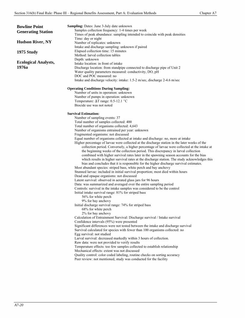
Section 316(b) Final Rule: Phase III – Regional Benefits Assessment, Part A: Evaluation Methods Chapter A7
A7-20
Bowline Point Generating Station Hudson River, NY 1975 Study Ecological Analysts, 1976a
Sampling: Dates: June 3-July date unknown Samples collection frequency: 1-4 times per week Times of peak abundance: sampling intended to coincide with peak densities Time: day or night Number of replicates: unknown Intake and discharge sampling: unknown if paired Elapsed collection time: 15 minutes Method: larval collection tables Depth: unknown Intake location: in front of intake Discharge location: from standpipe connected to discharge pipe of Unit 2 Water quality parameters measured: conductivity, DO, pH DOC and POC measured: no Intake and discharge velocity: intake: 1.5-2 m/sec, discharge 2-4.6 m/sec
Operating Conditions During Sampling: Number of units in operation: unknown Number of pumps in operation: unknown Temperature: )T range: 0.5-12.1 EC Biocide use was not noted
Survival Estimation: Number of sampling events: 37 Total number of samples collected: 400 Total number of organisms collected: 4,643 Number of organisms entrained per year: unknown Fragmented organisms: not discussed Equal number of organisms collected at intake and discharge: no, more at intake Higher percentage of larvae were collected at the discharge station in the later weeks of the
collection period. Conversely, a higher percentage of larvae were collected at the intake at the beginning weeks of the collection period. This discrepancy in larval collection combined with higher survival rates later in the spawning season accounts for the bias which results in higher survival rates at the discharge station. The study acknowledges this bias and concludes that it is responsible for the higher discharge survival estimates.
Most abundant species: striped bass, white perch and bay anchovy Stunned larvae: included in initial survival proportion; most died within hours Dead and opaque organisms: not discussed Latent survival: observed in aerated glass jars for 96 hours Data: was summarized and averaged over the entire sampling period Controls: survival in the intake samples was considered to be the control Initial intake survival range: 81% for striped bass
56% for white perch 9% for bay anchovy
Initial discharge survival range: 74% for striped bass 68% for white perch 2% for bay anchovy
Calculation of Entrainment Survival: Discharge survival / Intake survival Confidence intervals (95%) were presented Significant differences were not tested between the intake and discharge survival Survival calculated for species with fewer than 100 organisms collected: no Egg survival: not studied Larval survival: decreased markedly within 3 hours of collection. Raw data: were not provided to verify results Temperature effects: too few samples collected to establish relationship Mechanical effects: extent was not discussed Quality control: color coded labeling, routine checks on sorting accuracy Peer review: not mentioned, study was conducted for the facility
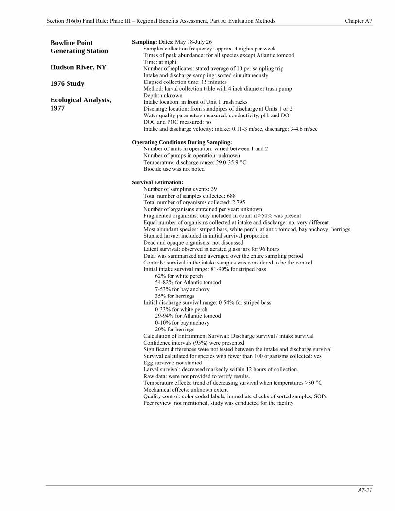
Section 316(b) Final Rule: Phase III – Regional Benefits Assessment, Part A: Evaluation Methods Chapter A7
A7-21
Bowline Point Generating Station Hudson River, NY 1976 Study Ecological Analysts, 1977
Sampling: Dates: May 18-July 26 Samples collection frequency: approx. 4 nights per week Times of peak abundance: for all species except Atlantic tomcod Time: at night Number of replicates: stated average of 10 per sampling trip Intake and discharge sampling: sorted simultaneously Elapsed collection time: 15 minutes Method: larval collection table with 4 inch diameter trash pump Depth: unknown Intake location: in front of Unit 1 trash racks Discharge location: from standpipes of discharge at Units 1 or 2 Water quality parameters measured: conductivity, pH, and DO DOC and POC measured: no Intake and discharge velocity: intake: 0.11-3 m/sec, discharge: 3-4.6 m/sec
Operating Conditions During Sampling: Number of units in operation: varied between 1 and 2 Number of pumps in operation: unknown Temperature: discharge range: 29.0-35.9 EC Biocide use was not noted
Survival Estimation: Number of sampling events: 39 Total number of samples collected: 688 Total number of organisms collected: 2,795 Number of organisms entrained per year: unknown Fragmented organisms: only included in count if >50% was present Equal number of organisms collected at intake and discharge: no, very different Most abundant species: striped bass, white perch, atlantic tomcod, bay anchovy, herrings Stunned larvae: included in initial survival proportion Dead and opaque organisms: not discussed Latent survival: observed in aerated glass jars for 96 hours Data: was summarized and averaged over the entire sampling period Controls: survival in the intake samples was considered to be the control Initial intake survival range: 81-90% for striped bass
62% for white perch 54-82% for Atlantic tomcod 7-53% for bay anchovy 35% for herrings
Initial discharge survival range: 0-54% for striped bass 0-33% for white perch 29-94% for Atlantic tomcod 0-10% for bay anchovy 20% for herrings
Calculation of Entrainment Survival: Discharge survival / intake survival Confidence intervals (95%) were presented Significant differences were not tested between the intake and discharge survival Survival calculated for species with fewer than 100 organisms collected: yes Egg survival: not studied Larval survival: decreased markedly within 12 hours of collection. Raw data: were not provided to verify results. Temperature effects: trend of decreasing survival when temperatures >30 EC Mechanical effects: unknown extent Quality control: color coded labels, immediate checks of sorted samples, SOPs Peer review: not mentioned, study was conducted for the facility
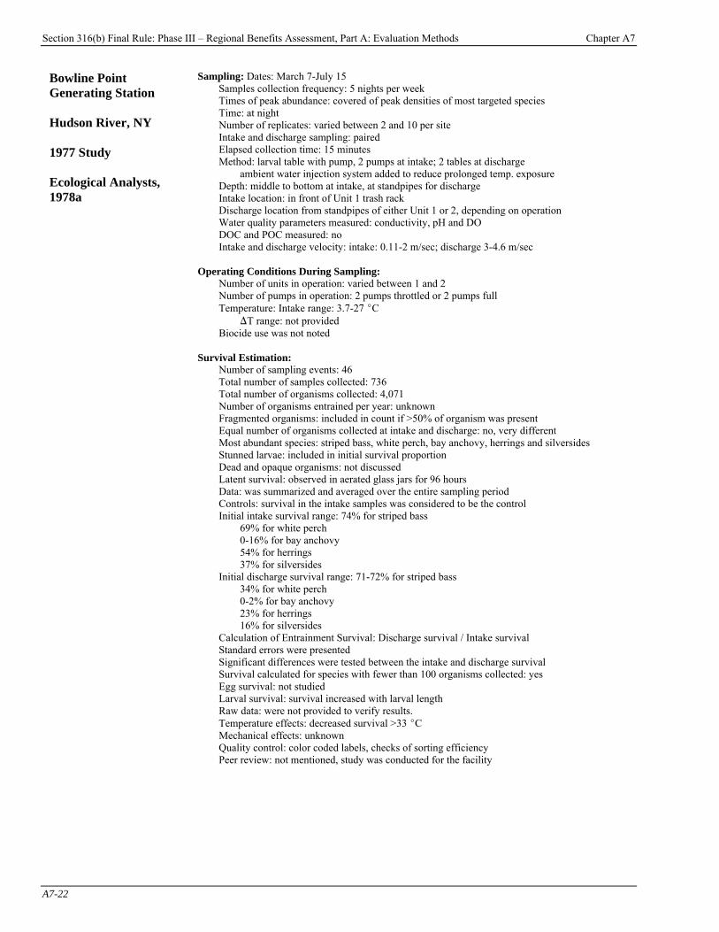
Section 316(b) Final Rule: Phase III – Regional Benefits Assessment, Part A: Evaluation Methods Chapter A7
A7-22
Bowline Point Generating Station Hudson River, NY 1977 Study Ecological Analysts, 1978a
Sampling: Dates: March 7-July 15 Samples collection frequency: 5 nights per week Times of peak abundance: covered of peak densities of most targeted species Time: at night Number of replicates: varied between 2 and 10 per site Intake and discharge sampling: paired Elapsed collection time: 15 minutes Method: larval table with pump, 2 pumps at intake; 2 tables at discharge
ambient water injection system added to reduce prolonged temp. exposure Depth: middle to bottom at intake, at standpipes for discharge Intake location: in front of Unit 1 trash rack Discharge location from standpipes of either Unit 1 or 2, depending on operation Water quality parameters measured: conductivity, pH and DO DOC and POC measured: no Intake and discharge velocity: intake: 0.11-2 m/sec; discharge 3-4.6 m/sec
Operating Conditions During Sampling: Number of units in operation: varied between 1 and 2 Number of pumps in operation: 2 pumps throttled or 2 pumps full Temperature: Intake range: 3.7-27 EC
)T range: not provided Biocide use was not noted
Survival Estimation: Number of sampling events: 46 Total number of samples collected: 736 Total number of organisms collected: 4,071 Number of organisms entrained per year: unknown Fragmented organisms: included in count if >50% of organism was present Equal number of organisms collected at intake and discharge: no, very different Most abundant species: striped bass, white perch, bay anchovy, herrings and silversides Stunned larvae: included in initial survival proportion Dead and opaque organisms: not discussed Latent survival: observed in aerated glass jars for 96 hours Data: was summarized and averaged over the entire sampling period Controls: survival in the intake samples was considered to be the control Initial intake survival range: 74% for striped bass
69% for white perch 0-16% for bay anchovy 54% for herrings 37% for silversides
Initial discharge survival range: 71-72% for striped bass 34% for white perch 0-2% for bay anchovy 23% for herrings 16% for silversides
Calculation of Entrainment Survival: Discharge survival / Intake survival Standard errors were presented Significant differences were tested between the intake and discharge survival Survival calculated for species with fewer than 100 organisms collected: yes Egg survival: not studied Larval survival: survival increased with larval length Raw data: were not provided to verify results. Temperature effects: decreased survival >33 EC Mechanical effects: unknown Quality control: color coded labels, checks of sorting efficiency Peer review: not mentioned, study was conducted for the facility
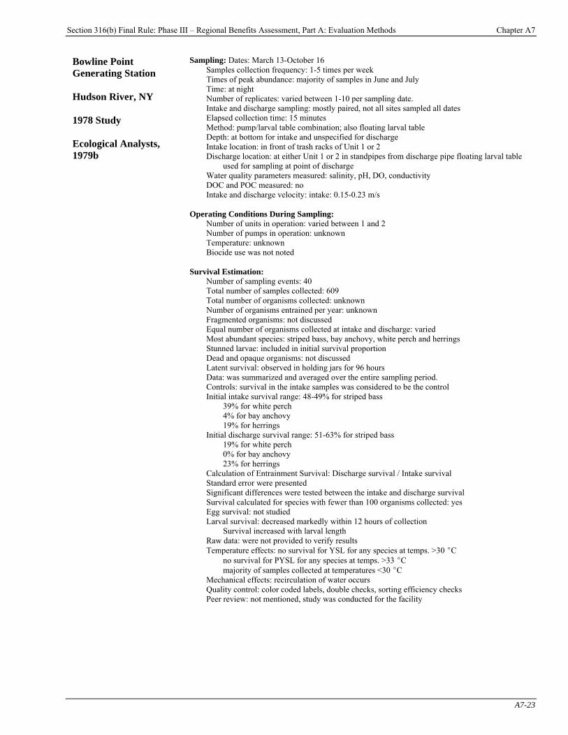
Section 316(b) Final Rule: Phase III – Regional Benefits Assessment, Part A: Evaluation Methods Chapter A7
A7-23
Bowline Point Generating Station Hudson River, NY 1978 Study Ecological Analysts, 1979b
Sampling: Dates: March 13-October 16 Samples collection frequency: 1-5 times per week Times of peak abundance: majority of samples in June and July Time: at night Number of replicates: varied between 1-10 per sampling date. Intake and discharge sampling: mostly paired, not all sites sampled all dates Elapsed collection time: 15 minutes Method: pump/larval table combination; also floating larval table Depth: at bottom for intake and unspecified for discharge Intake location: in front of trash racks of Unit 1 or 2 Discharge location: at either Unit 1 or 2 in standpipes from discharge pipe floating larval table
used for sampling at point of discharge Water quality parameters measured: salinity, pH, DO, conductivity DOC and POC measured: no Intake and discharge velocity: intake: 0.15-0.23 m/s
Operating Conditions During Sampling:
Number of units in operation: varied between 1 and 2 Number of pumps in operation: unknown Temperature: unknown Biocide use was not noted
Survival Estimation: Number of sampling events: 40 Total number of samples collected: 609 Total number of organisms collected: unknown Number of organisms entrained per year: unknown Fragmented organisms: not discussed Equal number of organisms collected at intake and discharge: varied Most abundant species: striped bass, bay anchovy, white perch and herrings Stunned larvae: included in initial survival proportion Dead and opaque organisms: not discussed Latent survival: observed in holding jars for 96 hours Data: was summarized and averaged over the entire sampling period. Controls: survival in the intake samples was considered to be the control Initial intake survival range: 48-49% for striped bass
39% for white perch 4% for bay anchovy 19% for herrings
Initial discharge survival range: 51-63% for striped bass 19% for white perch 0% for bay anchovy 23% for herrings
Calculation of Entrainment Survival: Discharge survival / Intake survival Standard error were presented Significant differences were tested between the intake and discharge survival Survival calculated for species with fewer than 100 organisms collected: yes Egg survival: not studied Larval survival: decreased markedly within 12 hours of collection
Survival increased with larval length Raw data: were not provided to verify results Temperature effects: no survival for YSL for any species at temps. >30 EC
no survival for PYSL for any species at temps. >33 EC majority of samples collected at temperatures <30 EC
Mechanical effects: recirculation of water occurs Quality control: color coded labels, double checks, sorting efficiency checks Peer review: not mentioned, study was conducted for the facility
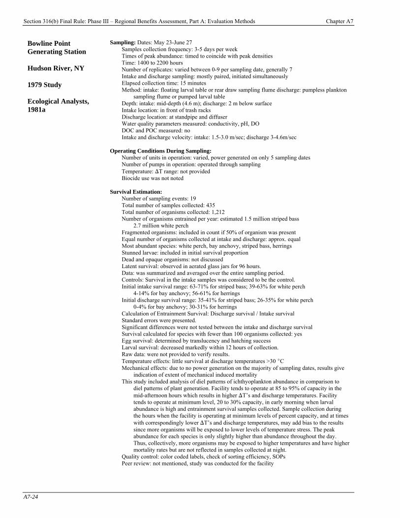
Section 316(b) Final Rule: Phase III – Regional Benefits Assessment, Part A: Evaluation Methods Chapter A7
A7-24
Bowline Point Generating Station Hudson River, NY 1979 Study Ecological Analysts, 1981a
Sampling: Dates: May 23-June 27 Samples collection frequency: 3-5 days per week Times of peak abundance: timed to coincide with peak densities Time: 1400 to 2200 hours Number of replicates: varied between 0-9 per sampling date, generally 7 Intake and discharge sampling: mostly paired, initiated simultaneously Elapsed collection time: 15 minutes Method: intake: floating larval table or rear draw sampling flume discharge: pumpless plankton
sampling flume or pumped larval table Depth: intake: mid-depth (4.6 m); discharge: 2 m below surface Intake location: in front of trash racks Discharge location: at standpipe and diffuser Water quality parameters measured: conductivity, pH, DO DOC and POC measured: no Intake and discharge velocity: intake: 1.5-3.0 m/sec; discharge 3-4.6m/sec
Operating Conditions During Sampling: Number of units in operation: varied, power generated on only 5 sampling dates Number of pumps in operation: operated through sampling Temperature: )T range: not provided Biocide use was not noted
Survival Estimation: Number of sampling events: 19 Total number of samples collected: 435 Total number of organisms collected: 1,212 Number of organisms entrained per year: estimated 1.5 million striped bass
2.7 million white perch Fragmented organisms: included in count if 50% of organism was present Equal number of organisms collected at intake and discharge: approx. equal Most abundant species: white perch, bay anchovy, striped bass, herrings Stunned larvae: included in initial survival proportion Dead and opaque organisms: not discussed Latent survival: observed in aerated glass jars for 96 hours. Data: was summarized and averaged over the entire sampling period. Controls: Survival in the intake samples was considered to be the control. Initial intake survival range: 63-71% for striped bass; 39-63% for white perch
4-14% for bay anchovy; 56-61% for herrings Initial discharge survival range: 35-41% for striped bass; 26-35% for white perch
0-4% for bay anchovy; 30-31% for herrings Calculation of Entrainment Survival: Discharge survival / Intake survival Standard errors were presented. Significant differences were not tested between the intake and discharge survival Survival calculated for species with fewer than 100 organisms collected: yes Egg survival: determined by translucency and hatching success Larval survival: decreased markedly within 12 hours of collection. Raw data: were not provided to verify results. Temperature effects: little survival at discharge temperatures >30 EC Mechanical effects: due to no power generation on the majority of sampling dates, results give
indication of extent of mechanical induced mortality This study included analysis of diel patterns of ichthyoplankton abundance in comparison to
diel patterns of plant generation. Facility tends to operate at 85 to 95% of capacity in the mid-afternoon hours which results in higher )T’s and discharge temperatures. Facility tends to operate at minimum level, 20 to 30% capacity, in early morning when larval abundance is high and entrainment survival samples collected. Sample collection during the hours when the facility is operating at minimum levels of percent capacity, and at times with correspondingly lower )T’s and discharge temperatures, may add bias to the results since more organisms will be exposed to lower levels of temperature stress. The peak abundance for each species is only slightly higher than abundance throughout the day. Thus, collectively, more organisms may be exposed to higher temperatures and have higher mortality rates but are not reflected in samples collected at night.
Quality control: color coded labels, check of sorting efficiency, SOPs Peer review: not mentioned, study was conducted for the facility
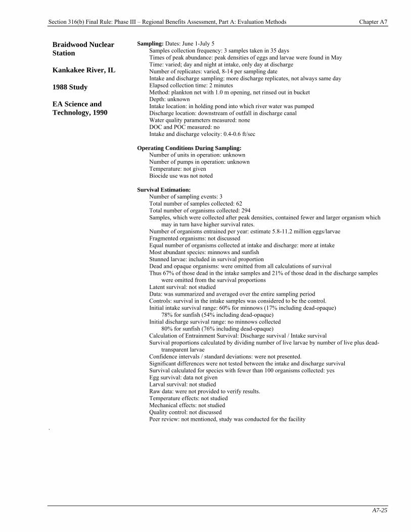
Section 316(b) Final Rule: Phase III – Regional Benefits Assessment, Part A: Evaluation Methods Chapter A7
A7-25
Braidwood Nuclear Station Kankakee River, IL 1988 Study EA Science and Technology, 1990
Sampling: Dates: June 1-July 5 Samples collection frequency: 3 samples taken in 35 days Times of peak abundance: peak densities of eggs and larvae were found in May Time: varied; day and night at intake, only day at discharge Number of replicates: varied, 8-14 per sampling date Intake and discharge sampling: more discharge replicates, not always same day Elapsed collection time: 2 minutes Method: plankton net with 1.0 m opening, net rinsed out in bucket Depth: unknown Intake location: in holding pond into which river water was pumped Discharge location: downstream of outfall in discharge canal Water quality parameters measured: none DOC and POC measured: no Intake and discharge velocity: 0.4-0.6 ft/sec
Operating Conditions During Sampling: Number of units in operation: unknown Number of pumps in operation: unknown Temperature: not given Biocide use was not noted
Survival Estimation: Number of sampling events: 3 Total number of samples collected: 62 Total number of organisms collected: 294 Samples, which were collected after peak densities, contained fewer and larger organism which
may in turn have higher survival rates. Number of organisms entrained per year: estimate 5.8-11.2 million eggs/larvae Fragmented organisms: not discussed Equal number of organisms collected at intake and discharge: more at intake Most abundant species: minnows and sunfish Stunned larvae: included in survival proportion Dead and opaque organisms: were omitted from all calculations of survival Thus 67% of those dead in the intake samples and 21% of those dead in the discharge samples
were omitted from the survival proportions Latent survival: not studied Data: was summarized and averaged over the entire sampling period Controls: survival in the intake samples was considered to be the control. Initial intake survival range: 60% for minnows (17% including dead-opaque)
78% for sunfish (54% including dead-opaque) Initial discharge survival range: no minnows collected
80% for sunfish (76% including dead-opaque) Calculation of Entrainment Survival: Discharge survival / Intake survival Survival proportions calculated by dividing number of live larvae by number of live plus dead-
transparent larvae Confidence intervals / standard deviations: were not presented. Significant differences were not tested between the intake and discharge survival Survival calculated for species with fewer than 100 organisms collected: yes Egg survival: data not given Larval survival: not studied Raw data: were not provided to verify results. Temperature effects: not studied Mechanical effects: not studied Quality control: not discussed Peer review: not mentioned, study was conducted for the facility
.
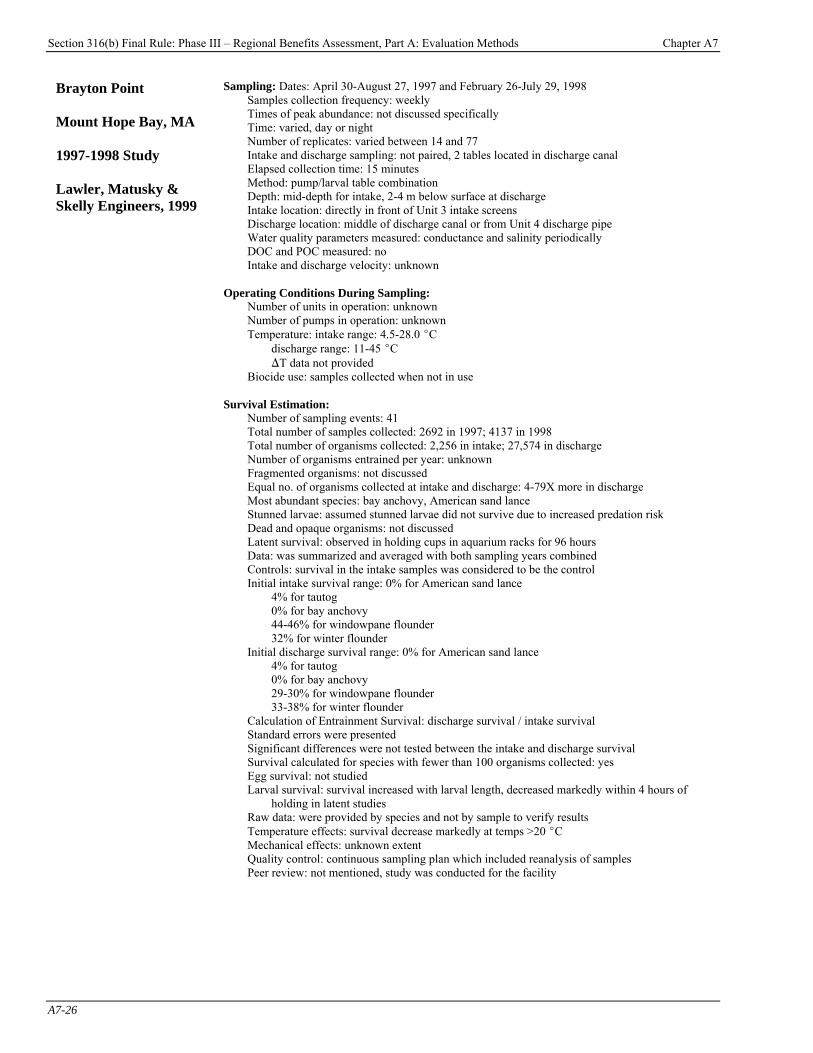
Section 316(b) Final Rule: Phase III – Regional Benefits Assessment, Part A: Evaluation Methods Chapter A7
A7-26
Brayton Point Mount Hope Bay, MA 1997-1998 Study Lawler, Matusky & Skelly Engineers, 1999
Sampling: Dates: April 30-August 27, 1997 and February 26-July 29, 1998 Samples collection frequency: weekly Times of peak abundance: not discussed specifically Time: varied, day or night Number of replicates: varied between 14 and 77 Intake and discharge sampling: not paired, 2 tables located in discharge canal Elapsed collection time: 15 minutes Method: pump/larval table combination Depth: mid-depth for intake, 2-4 m below surface at discharge Intake location: directly in front of Unit 3 intake screens Discharge location: middle of discharge canal or from Unit 4 discharge pipe Water quality parameters measured: conductance and salinity periodically DOC and POC measured: no Intake and discharge velocity: unknown
Operating Conditions During Sampling: Number of units in operation: unknown Number of pumps in operation: unknown Temperature: intake range: 4.5-28.0 EC
discharge range: 11-45 EC )T data not provided
Biocide use: samples collected when not in use
Survival Estimation: Number of sampling events: 41 Total number of samples collected: 2692 in 1997; 4137 in 1998 Total number of organisms collected: 2,256 in intake; 27,574 in discharge Number of organisms entrained per year: unknown Fragmented organisms: not discussed Equal no. of organisms collected at intake and discharge: 4-79X more in discharge Most abundant species: bay anchovy, American sand lance Stunned larvae: assumed stunned larvae did not survive due to increased predation risk Dead and opaque organisms: not discussed Latent survival: observed in holding cups in aquarium racks for 96 hours Data: was summarized and averaged with both sampling years combined Controls: survival in the intake samples was considered to be the control Initial intake survival range: 0% for American sand lance
4% for tautog 0% for bay anchovy 44-46% for windowpane flounder 32% for winter flounder
Initial discharge survival range: 0% for American sand lance 4% for tautog 0% for bay anchovy 29-30% for windowpane flounder 33-38% for winter flounder
Calculation of Entrainment Survival: discharge survival / intake survival Standard errors were presented Significant differences were not tested between the intake and discharge survival Survival calculated for species with fewer than 100 organisms collected: yes Egg survival: not studied Larval survival: survival increased with larval length, decreased markedly within 4 hours of
holding in latent studies Raw data: were provided by species and not by sample to verify results Temperature effects: survival decrease markedly at temps >20 EC Mechanical effects: unknown extent Quality control: continuous sampling plan which included reanalysis of samples Peer review: not mentioned, study was conducted for the facility

Section 316(b) Final Rule: Phase III – Regional Benefits Assessment, Part A: Evaluation Methods Chapter A7
A7-27
Cayuga Generating Plant Wabash River, IN 1979 Study Ecological Analysts, 1980a
Sampling: Dates: May 17-31 and June 8-22 Samples collection frequency: daily Times of peak abundance: highest average densities sampled were June 8-10 Time: 1900 to 0300 hours Number of replicates: varied between 0-6 per sampling date. Intake and discharge sampling: simultaneous sampling, transit time = 36 mins Elapsed collection time: 15 minutes Method: pump / larval table collection system Depth: intake: 2 and 5 m below surface, discharge: 3-4 m below surface Intake location: in front of intake structure Discharge location: where discharge of Units 1 and 2 enter canal
also cooling tower discharge in discharge canal Water quality parameters measured: DO DOC and POC measured: no Intake and discharge velocity: unknown
Operating Conditions During Sampling: Number of units in operation: unknown Number of pumps in operation: varied, 2-4 Temperature: intake range: 17.6-24.3 EC
discharge range: 29.4-33.3 EC )T ranged from 8.4-11.8 EC
Biocide use: occurs daily, but ceased at least 2 hours before sampling
Survival Estimation: Number of sampling events: 24 Total number of samples collected: 80 Total number of organisms collected: 2,556 Number of organisms entrained per year: unknown Fragmented organisms: 13-14.6% were damaged Equal number of organisms collected at intake and discharge: more at intake Most abundant species: suckers, perches, carps, temperate basses Stunned larvae: included in initial survival proportion Dead and opaque organisms: not discussed Latent survival: 48 hour observation in aerated glass jars of filtered river water Data: was summarized and averaged over the entire sampling period Controls: survival in the intake samples was considered to be the control Initial intake survival range: 86-98% for suckers
28-92% for carps and minnows 50-86% for perches
Initial discharge survival range: 75-92% for suckers 12-74% for carps and minnows 43-69% for perches
Calculation of Entrainment Survival: Discharge survival/ Intake survival Confidence intervals: were not presented; standard errors were calculated standard error
sometime as high as survival Significant differences were tested between the intake and discharge survival Survival calculated for species with fewer than 100 organisms collected: yes Egg survival: not studied Larval survival: latent effects were not seen until 48 hours after collection Raw data: were provided to verify results Temperature effects: lower survival for all species at temperatures above 30 °C Mechanical effects: survival decreased when number of pumps increased Quality control: sorting efficiency checks and color coded labels Peer review: not mentioned, study was conducted for the facility
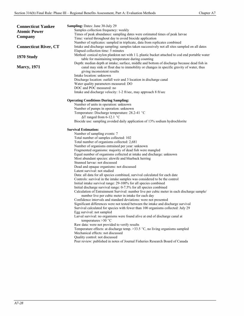
Section 316(b) Final Rule: Phase III – Regional Benefits Assessment, Part A: Evaluation Methods Chapter A7
A7-28
Connecticut Yankee Atomic Power Company Connecticut River, CT 1970 Study Marcy, 1971
Sampling: Dates: June 30-July 29 Samples collection frequency: weekly Times of peak abundance: sampling dates were estimated times of peak larvae Time: varied throughout day to avoid biocide application Number of replicates: sampled in triplicate, data from replicates combined Intake and discharge sampling: samples taken successively not all sites sampled on all dates Elapsed collection time: 5 minutes Method: conical nylon plankton net with 1 L plastic bucket attached to cod end portable water
table for maintaining temperature during counting Depth: median depth at intake; surface, middle and bottom of discharge because dead fish in
canal may sink or float due to immobility or changes in specific gravity of water, thus giving inconsistent results
Intake location: unknown Discharge location: outfall weir and 3 location in discharge canal Water quality parameters measured: DO DOC and POC measured: no Intake and discharge velocity: 1-2 ft/sec, may approach 8 ft/sec
Operating Conditions During Sampling: Number of units in operation: unknown Number of pumps in operation: unknown Temperature: Discharge temperature: 28.2-41 EC
)T ranged from 6-12.1 EC Biocide use: sampling avoided daily application of 13% sodium hydrochlorite
Survival Estimation: Number of sampling events: 7 Total number of samples collected: 102 Total number of organisms collected: 2,681 Number of organisms entrained per year: unknown Fragmented organisms: majority of dead fish were mangled Equal number of organisms collected at intake and discharge: unknown Most abundant species: alewife and blueback herring Stunned larvae: not discussed Dead and opaque organisms: not discussed Latent survival: not studied Data: all data for all species combined, survival calculated for each date Controls: survival in the intake samples was considered to be the control Initial intake survival range: 29-100% for all species combined Initial discharge survival range: 0-7.5% for all species combined Calculation of Entrainment Survival: number live per cubic meter in each discharge sample/
number live per cubic meter in intake for each day Confidence intervals and standard deviations: were not presented Significant differences were not tested between the intake and discharge survival Survival calculated for species with fewer than 100 organisms collected: July 29 Egg survival: not sampled Larval survival: no organisms were found alive at end of discharge canal at
temperatures >30 EC Raw data: were not provided to verify results Temperature effects: at discharge temp. >33.5 EC, no living organisms sampled Mechanical effects: not discussed Quality control: not discussed Peer review: published in notes of Journal Fisheries Research Board of Canada
Section 316(b) Final Rule: Phase III – Regional Benefits Assessment, Part A: Evaluation Methods Chapter A7
A7-29
Connecticut Yankee Atomic Power Company Connecticut River, CT 1971-1972 Study Marcy, 1973
Sampling: Dates: June 2-24, 1971 and June 27-July 13, 1972 (mechanical only) Samples collection frequency: approximately once per week Times of peak abundance: unknown Time: afternoons and evenings Number of replicates: three at each station although at three different depths data were
combined for each station Intake and discharge sampling: collected successively at the 5 sites Elapsed collection time: 5 minutes Method: conical nylon plankton net with 0.39 mm mesh and 1L plastic bucket Depth: surface, middle, and bottom Intake location: unknown Discharge location: below weir and 3 points along discharge canal Water quality parameters measured: none DOC and POC measured: no Intake and discharge velocity: 0.3-0.6 m/sec, may approach 2.4 m/sec
Operating Conditions During Sampling: Number of units in operation: unknown in 1971, no power generation in 1972 Number of pumps in operation: unknown Temperature: Intake temperature: 16-26 EC (1971); 19.9-28 EC (1972)
Discharge temperature: 29-35 EC (1971 only) )T ranged from 9-13 EC (1971 only)
Biocide use: 1972 study, chemical mortality indistinguishable from mechanical
Survival Estimation: Number of sampling events: 2 (1971) and 7 (1972) Total number of samples collected: 30 (1971) and 246 (1972) often 2-3 times as many samples
collected at discharge Total number of organisms collected: 1,068 (1971) and 10,271 (1972) Number of organisms entrained per year: unknown, estimated entrainment is 1.7-5.8% of
nonscreenable fish which pass facility Fragmented organisms: not discussed Equal no. of organisms collected at intake and discharge: 4X more in discharge lower numbers
collected at end of canal may be due to dead fish settling out of water column Most abundant species: alewife and blueback herring Stunned larvae: were included as live unless they had begun to turn opaque Dead and opaque organisms: only opaque organisms were counted as dead Latent survival: not studied Data: replicate data combined; survival calculated per sampling day Controls: survival in the intake samples was considered to be the control Initial intake survival range: 64-100% for all species sampled (1971) Initial discharge survival range: 0% for all species sampled (1971) Calculation of Entrainment Survival: number live per cubic meter in each discharge sample/
number live per cubic meter in intake for each day Confidence intervals and standard deviations were not presented. Significant differences were not tested between the intake and discharge survival Survival calculated for species with fewer than 100 organisms collected: yes Egg survival: none sampled Larval survival: no survival anywhere in discharge at temperatures >29 EC Raw data: were not provided to verify results Temperature effects: organisms exposed to elevated temp. for 50-100 min estimated as causing
20% of mortality most fish are dead at the end of the 1.14 mile canal Mechanical effects: 1972 study indicated that 72-87% is mechanical mortality Quality control: not discussed Peer review: published in Journal Fisheries Research Board of Canada
Section 316(b) Final Rule: Phase III – Regional Benefits Assessment, Part A: Evaluation Methods Chapter A7
A7-30
Contra Costa Power Plant San Joaquin River, CA 1976 Study Stevens and Finlayson, 1978
Sampling: Dates: April 28-July 10 Samples collection frequency: once per week Times of peak abundance: unknown Time: varied, about 25% of all samples collected at night Number of replicates: typically 3 Intake and discharge sampling: paired at closest time and temperature Elapsed collection time: 1-2 minutes Method: 505 micron mech conical nylon plankton net with 0.58 m plastic collecting tubes on
cod end; towed net on boat at 0.6 ft/sec Depth: mid-depth Intake location: at intake for units 6 and 7 Discharge location: at discharge for units 1-5 and units 6-7 Water quality parameters measured: none DOC and POC measured: no Intake and discharge velocity: unknown
Operating Conditions During Sampling: Number of units in operation: unknown Number of pumps in operation: unknown Temperature: Intake temperature: 19-30 EC Discharge temperature 19-38 EC Biocide use was not noted
Survival Estimation: Number of sampling events: 6 Total number of samples collected: unknown Total number of organisms collected: 966 (1,606 at north shore control) Number of organisms entrained per year: unknown Fragmented organisms: enumerated in one replicate tow higher proportion of unidentifiable
fragments in discharge Equal number of organisms collected at intake and discharge: more at intake Most abundant species: striped bass Stunned larvae: included in initial survival proportion Dead and opaque organisms: not discussed Latent survival: not studied Data: was summarized by mean larval length Controls: survival in the intake samples was considered to be the control additional control on
north shore to determine background mortality control site at north shore away from intake had lower mortality rates
Initial intake survival range: 33-90% for striped bass recirculated water may be cause of some intake mortality Initial discharge survival range: 0-50% for striped bass Calculation of Entrainment Survival: paired discharge survival divided by paired intake survival Confidence intervals and standard deviations were not presented. Significant differences were not tested between the intake and discharge survival Survival calculated for species with fewer than 100 organisms collected: yes Egg survival: not studied Larval survival: increased survival with greater larval length Raw data: were not provided to verify results Temperature effects: mortality increased with increase in discharge temperature higher
mortality with discharge temp. >31 and )T >7 EC linear regression showed that half died at temps >33.3 EC
0% survival at temperatures of 38 EC Mechanical effects: stated not as much of an effects as temperature Quality control: not discussed Peer review: study conducted by California Fish and Game with funds provided by facility
Section 316(b) Final Rule: Phase III – Regional Benefits Assessment, Part A: Evaluation Methods Chapter A7
A7-31
Danskammer Point Generating Station Hudson River, NY 1975 Study Ecological Analysts, 1976b
Sampling: Dates: May 29-November 18 Samples collection frequency: varied from once every 2 weeks to 4 times per week Times of peak abundance: increased frequency during spawning Time: varied, generally overnight Number of replicates: varied, ranged from 1 to 12 Intake and discharge sampling: usually paired Elapsed collection time: unknown Method: pump/larval table Depth: mid-depth for intake, unspecified for discharge Intake location: in canal in front of traveling screens Discharge location: outlet of Unit 3 to Hudson River Water quality parameters measured: none DOC and POC measured: no Intake and discharge velocity: unknown
Operating Conditions During Sampling: Number of units in operation: unknown Number of pumps in operation: varied between 1 and 2 Temperature: Intake temperature range: 21-26 EC
Discharge temperature range: not provided )T ranged from 0-10 EC
Biocide use not used during sampling; noted that chlorination will reduce survival
Survival Estimation: Number of sampling events: 29 Total number of samples collected: 372 Total number of organisms collected: 1,655 Number of organisms entrained per year: unknown Fragmented organisms: not discussed Equal no. of organisms collected at intake / discharge: up to 2X more in discharge Most abundant species: herrings, striped bass and white perch Stunned larvae: included in initial survival proportion Dead and opaque organisms: not discussed Latent survival: observed in aerated glass jars for 96 hours Data: was summarized and averaged over the entire sampling period Controls: survival in the intake samples was considered to be the control Initial intake survival range: 0-50% for striped bass
33-100% for white perch 63-100% for herrings
Initial discharge survival range: 0-39% for striped bass 38-80% for white perch 20-22% for herrings
Calculation of Entrainment Survival: Discharge survival / Intake survival Confidence intervals and standard deviations: were not presented. Significant differences were tested between the intake and discharge survival Significantly lower survival in discharge: herring PYSL Survival calculated for species with fewer than 100 organisms collected: yes Egg survival: none collected Larval survival: decreased markedly within 3 hours of collection. Raw data: were not provided to verify results Temperature effects: significantly lower survival when )T >10 EC and discharge
temperature >30 EC Mechanical effects: not discussed Quality control: samples double checked and data entry monitored Peer review: not mentioned, study was conducted for the facility
Section 316(b) Final Rule: Phase III – Regional Benefits Assessment, Part A: Evaluation Methods Chapter A7
A7-32
Fort Calhoun Nuclear Station Missouri River, NE 1973-1977 study Carter, 1978
Sampling: Dates: October 1973-June 1977 Samples collection frequency: 5-24 times per year Times of peak abundance: same frequency all year round Time: unknown Number of replicates: unknown Intake and discharge sampling: unknown if timing was paired Elapsed collection time: unknown Method: plankton net with 571 :m mesh and 0.75 m diameter Depth: unknown Intake location: in river near intake Discharge location: near discharge in river immediately downstream of intake Water quality parameters measured: none DOC and POC measured: no Intake and discharge velocity: unknown
Operating Conditions During Sampling: Number of units in operation: varied, 25-97% of full power or shut down Number of pumps in operation: unknown Temperature: Discharge temperature: 27.0-36.9 EC during summer samples
)T ranged from 0.6-13.5 EC Biocide use: unspecified number of samples collected during chlorination
Survival Estimation: Number of sampling events: 89 (16 when facility was shut down) Total number of samples collected: unknown Total number of organisms collected: 24,535 macroinvertebrates Number of organisms entrained per year: unknown Fragmented organisms: not discussed Equal number of organisms collected at intake and discharge: no, varied Most abundant species: Ephemeroptera, Hydropsychidae, Chironomidae Stunned larvae: macroinvertebrates studied Dead and opaque organisms: not discussed Latent survival: not studied Data: was summarized and averaged over entire sampling period Controls: Survival in the intake samples was considered to be the control Initial intake survival range: 12-26% for Ephemeroptera
42-51% for Hydropsychidae 35-60% for Chironomidae
Initial discharge survival range: 18-32% for Ephemeroptera 47-56% for Hydropsychidae 43-66% for Chironomidae
Calculation of Entrainment Survival: Average differential mortality Confidence intervals / standard deviations: were calculated but not presented Significant differences were not tested between the intake and discharge survival Survival calculated for species with fewer than 100 organisms collected: yes Egg survival: not collected Larval survival: macroinvertebrates only were studied Raw data: were not provided to verify results Temperature effects: discussed but data not presented Mechanical effects: studied during 16 dates when facility was shut down Quality control: unknown Peer review: not mentioned, study was conducted for the facility
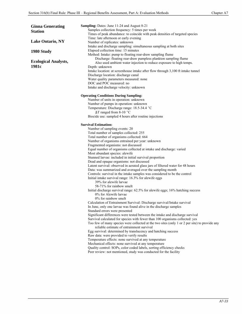
Section 316(b) Final Rule: Phase III – Regional Benefits Assessment, Part A: Evaluation Methods Chapter A7
A7-33
Ginna Generating Station Lake Ontario, NY 1980 Study Ecological Analysts, 1981c
Sampling: Dates: June 11-24 and August 8-21 Samples collection frequency: 5 times per week Times of peak abundance: to coincide with peak densities of targeted species Time: late afternoon or early evening Number of replicates: unknown Intake and discharge sampling: simultaneous sampling at both sites Elapsed collection time: 15 minutes Method: Intake: pump to floating rear-draw sampling flume
Discharge: floating rear-draw pumpless plankton sampling flume Also used ambient water injection to reduce exposure to high temps.
Depth: unknown Intake location: at screenhouse intake after flow through 3,100 ft intake tunnel Discharge location: discharge canal Water quality parameters measured: none DOC and POC measured: no Intake and discharge velocity: unknown
Operating Conditions During Sampling: Number of units in operation: unknown Number of pumps in operation: unknown Temperature: Discharge range: 18.5-34.4 EC
)T ranged from 8-10 EC Biocide use: sampled 4 hours after routine injections
Survival Estimation: Number of sampling events: 20 Total number of samples collected: 255 Total number of organisms collected: 664 Number of organisms entrained per year: unknown Fragmented organisms: not discussed Equal number of organisms collected at intake and discharge: varied Most abundant species: alewife Stunned larvae: included in initial survival proportion Dead and opaque organisms: not discussed Latent survival: observed in aerated glass jars of filtered water for 48 hours Data: was summarized and averaged over the sampling month Controls: survival in the intake samples was considered to be the control Initial intake survival range: 16.3% for alewife eggs
39% for alewife larvae 58-71% for rainbow smelt
Initial discharge survival range: 62.5% for alewife eggs; 16% hatching success 0% for Alewife larvae 0% for rainbow smelt
Calculation of Entrainment Survival: Discharge survival/Intake survival In June, only one larvae was found alive in the discharge samples Standard errors were presented Significant differences were tested between the intake and discharge survival Survival calculated for species with fewer than 100 organisms collected: yes Too few of many species were collected at the two sites (only 1 or 2 per site) to provide any
reliable estimate of entrainment survival Egg survival: determined by translucency and hatching success Raw data: were provided to verify results Temperature effects: none survived at any temperature Mechanical effects: none survived at any temperature Quality control: SOPs, color coded labels, sorting efficiency checks Peer review: not mentioned, study was conducted for the facility
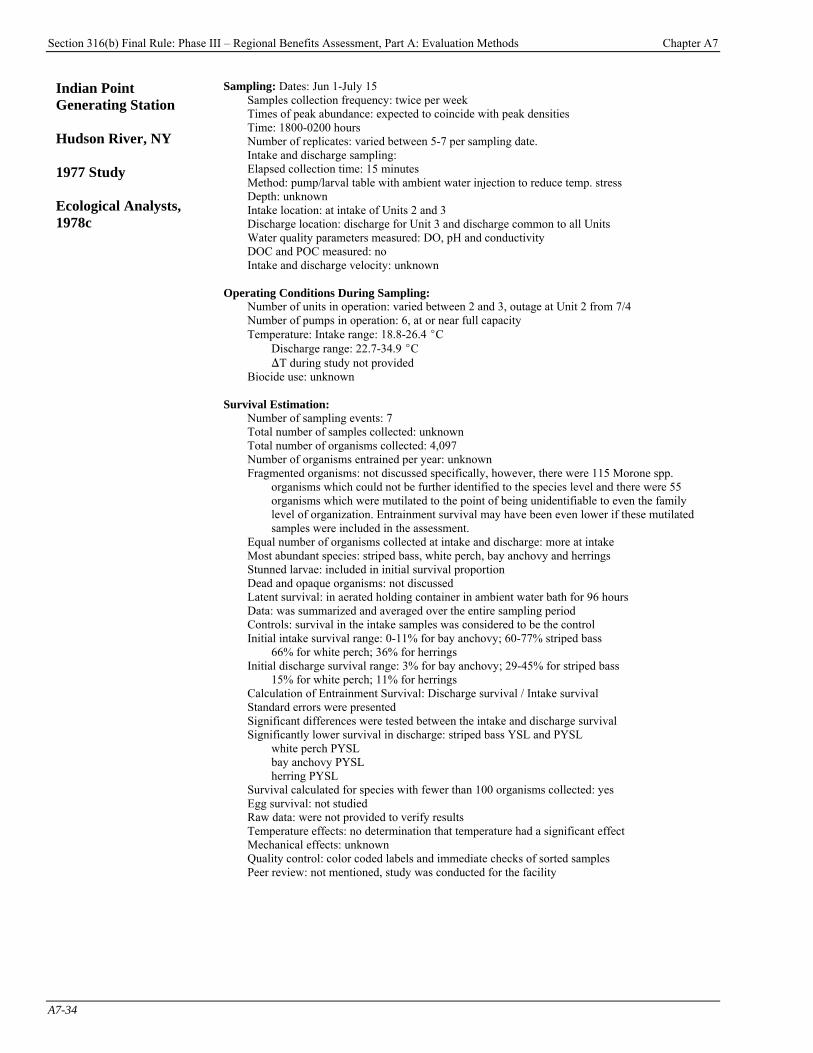
Section 316(b) Final Rule: Phase III – Regional Benefits Assessment, Part A: Evaluation Methods Chapter A7
A7-34
Indian Point Generating Station Hudson River, NY 1977 Study Ecological Analysts, 1978c
Sampling: Dates: Jun 1-July 15 Samples collection frequency: twice per week Times of peak abundance: expected to coincide with peak densities Time: 1800-0200 hours Number of replicates: varied between 5-7 per sampling date. Intake and discharge sampling: Elapsed collection time: 15 minutes Method: pump/larval table with ambient water injection to reduce temp. stress Depth: unknown Intake location: at intake of Units 2 and 3 Discharge location: discharge for Unit 3 and discharge common to all Units Water quality parameters measured: DO, pH and conductivity DOC and POC measured: no Intake and discharge velocity: unknown
Operating Conditions During Sampling: Number of units in operation: varied between 2 and 3, outage at Unit 2 from 7/4 Number of pumps in operation: 6, at or near full capacity Temperature: Intake range: 18.8-26.4 EC
Discharge range: 22.7-34.9 EC )T during study not provided
Biocide use: unknown
Survival Estimation: Number of sampling events: 7 Total number of samples collected: unknown Total number of organisms collected: 4,097 Number of organisms entrained per year: unknown Fragmented organisms: not discussed specifically, however, there were 115 Morone spp.
organisms which could not be further identified to the species level and there were 55 organisms which were mutilated to the point of being unidentifiable to even the family level of organization. Entrainment survival may have been even lower if these mutilated samples were included in the assessment.
Equal number of organisms collected at intake and discharge: more at intake Most abundant species: striped bass, white perch, bay anchovy and herrings Stunned larvae: included in initial survival proportion Dead and opaque organisms: not discussed Latent survival: in aerated holding container in ambient water bath for 96 hours Data: was summarized and averaged over the entire sampling period Controls: survival in the intake samples was considered to be the control Initial intake survival range: 0-11% for bay anchovy; 60-77% striped bass
66% for white perch; 36% for herrings Initial discharge survival range: 3% for bay anchovy; 29-45% for striped bass
15% for white perch; 11% for herrings Calculation of Entrainment Survival: Discharge survival / Intake survival Standard errors were presented Significant differences were tested between the intake and discharge survival Significantly lower survival in discharge: striped bass YSL and PYSL
white perch PYSL bay anchovy PYSL herring PYSL
Survival calculated for species with fewer than 100 organisms collected: yes Egg survival: not studied Raw data: were not provided to verify results Temperature effects: no determination that temperature had a significant effect Mechanical effects: unknown Quality control: color coded labels and immediate checks of sorted samples Peer review: not mentioned, study was conducted for the facility

Section 316(b) Final Rule: Phase III – Regional Benefits Assessment, Part A: Evaluation Methods Chapter A7
A7-35
Indian Point Generating Station Hudson River, NY 1978 Study Ecological Analysts, 1979c
Sampling: Dates: May 1-July 12 Samples collection frequency: 2 consecutive days per week Times of peak abundance: coincided with spawning of targeted species Time: 1800-0200 hours Number of replicates: approximately 6 per date Intake and discharge sampling: simultaneous Elapsed collection time: 15 minutes Method: pump/ larval table with ambient water injection Depth: 1-3 m below surface, approximately mid-depth Intake location: Unit 2 and 3 intake Discharge location: Unit 2 and 3 discharge, discharge point common to all units Water quality parameters measured: conductivity, pH and DO DOC and POC measured: no Intake and discharge velocity: unknown
Operating Conditions During Sampling: Number of units in operation: varied between 1 and 2 Number of pumps in operation: varied between 5-11, near full capacity Temperature: Intake range: 11.2-24.3 EC
Discharge range: 19-36 EC )T ranged from 9-12 EC
Biocide use was not noted
Survival Estimation: Number of sampling events: 22 Total number of samples collected: unknown Total number of organisms collected: 4,496 Number of organisms entrained per year: unknown Fragmented organisms: not discussed Equal number of organisms collected at intake and discharge: more at discharge Most abundant species: striped bass, white perch, bay anchovy and herrings Stunned larvae: included in initial survival proportion Dead and opaque organisms: not discussed Latent survival: observed in aerated glass jars for 96 hours Data: was summarized and averaged over the entire sampling period Controls: survival in the intake samples was considered to be the control Initial intake survival range: 26-48% for striped bass; 15-48% for white perch
18% for herring; 2% for bay anchovy Initial discharge survival range: 0-34% for striped bass; 0-37% for white perch
0-8% for herring; 0% for bay anchovy Calculation of Entrainment Survival: Discharge survival/ Intake survival Standard errors were presented Significant differences were tested between the intake and discharge survival Significantly lower survival at discharge: striped bass YSL, PYSL and juveniles
white perch PYSL herring PYSL
Survival calculated for species with fewer than 100 organisms collected: yes Egg survival: none were alive in either the intake or discharge samples Larval survival: decreased markedly within 24 hours of collection. Raw data: were not provided to verify results Temperature effects: at temps. >30 EC, no striped bass or white perch survived also 0%
survived when both Unit 2 and 3 were running Mechanical effects: not discussed Quality control: sorting efficiency checks, color coded labeling, SOPs Peer review: not mentioned, study was conducted for the facility
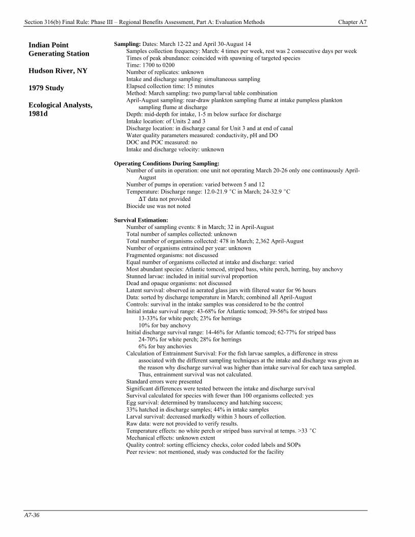
Section 316(b) Final Rule: Phase III – Regional Benefits Assessment, Part A: Evaluation Methods Chapter A7
A7-36
Indian Point Generating Station Hudson River, NY 1979 Study Ecological Analysts, 1981d
Sampling: Dates: March 12-22 and April 30-August 14 Samples collection frequency: March: 4 times per week, rest was 2 consecutive days per week Times of peak abundance: coincided with spawning of targeted species Time: 1700 to 0200 Number of replicates: unknown Intake and discharge sampling: simultaneous sampling Elapsed collection time: 15 minutes Method: March sampling: two pump/larval table combination April-August sampling: rear-draw plankton sampling flume at intake pumpless plankton
sampling flume at discharge Depth: mid-depth for intake, 1-5 m below surface for discharge Intake location: of Units 2 and 3 Discharge location: in discharge canal for Unit 3 and at end of canal Water quality parameters measured: conductivity, pH and DO DOC and POC measured: no Intake and discharge velocity: unknown
Operating Conditions During Sampling: Number of units in operation: one unit not operating March 20-26 only one continuously April-
August Number of pumps in operation: varied between 5 and 12 Temperature: Discharge range: 12.0-21.9 EC in March; 24-32.9 EC
)T data not provided Biocide use was not noted
Survival Estimation: Number of sampling events: 8 in March; 32 in April-August Total number of samples collected: unknown Total number of organisms collected: 478 in March; 2,362 April-August Number of organisms entrained per year: unknown Fragmented organisms: not discussed Equal number of organisms collected at intake and discharge: varied Most abundant species: Atlantic tomcod, striped bass, white perch, herring, bay anchovy Stunned larvae: included in initial survival proportion Dead and opaque organisms: not discussed Latent survival: observed in aerated glass jars with filtered water for 96 hours Data: sorted by discharge temperature in March; combined all April-August Controls: survival in the intake samples was considered to be the control Initial intake survival range: 43-68% for Atlantic tomcod; 39-56% for striped bass
13-33% for white perch; 23% for herrings 10% for bay anchovy
Initial discharge survival range: 14-46% for Atlantic tomcod; 62-77% for striped bass 24-70% for white perch; 28% for herrings 6% for bay anchovies
Calculation of Entrainment Survival: For the fish larvae samples, a difference in stress associated with the different sampling techniques at the intake and discharge was given as the reason why discharge survival was higher than intake survival for each taxa sampled. Thus, entrainment survival was not calculated.
Standard errors were presented Significant differences were tested between the intake and discharge survival Survival calculated for species with fewer than 100 organisms collected: yes Egg survival: determined by translucency and hatching success; 33% hatched in discharge samples; 44% in intake samples Larval survival: decreased markedly within 3 hours of collection. Raw data: were not provided to verify results. Temperature effects: no white perch or striped bass survival at temps. >33 EC Mechanical effects: unknown extent Quality control: sorting efficiency checks, color coded labels and SOPs Peer review: not mentioned, study was conducted for the facility
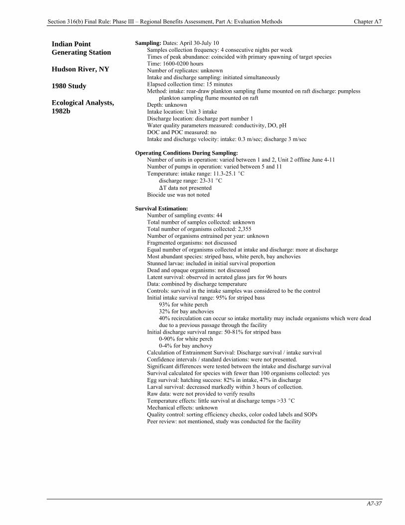
Section 316(b) Final Rule: Phase III – Regional Benefits Assessment, Part A: Evaluation Methods Chapter A7
A7-37
Indian Point Generating Station Hudson River, NY 1980 Study Ecological Analysts, 1982b
Sampling: Dates: April 30-July 10 Samples collection frequency: 4 consecutive nights per week Times of peak abundance: coincided with primary spawning of target species Time: 1600-0200 hours Number of replicates: unknown Intake and discharge sampling: initiated simultaneously Elapsed collection time: 15 minutes Method: intake: rear-draw plankton sampling flume mounted on raft discharge: pumpless
plankton sampling flume mounted on raft Depth: unknown Intake location: Unit 3 intake Discharge location: discharge port number 1 Water quality parameters measured: conductivity, DO, pH DOC and POC measured: no Intake and discharge velocity: intake: 0.3 m/sec; discharge 3 m/sec
Operating Conditions During Sampling: Number of units in operation: varied between 1 and 2, Unit 2 offline June 4-11 Number of pumps in operation: varied between 5 and 11 Temperature: intake range: 11.3-25.1 EC
discharge range: 23-31 EC )T data not presented
Biocide use was not noted
Survival Estimation: Number of sampling events: 44 Total number of samples collected: unknown Total number of organisms collected: 2,355 Number of organisms entrained per year: unknown Fragmented organisms: not discussed Equal number of organisms collected at intake and discharge: more at discharge Most abundant species: striped bass, white perch, bay anchovies Stunned larvae: included in initial survival proportion Dead and opaque organisms: not discussed Latent survival: observed in aerated glass jars for 96 hours Data: combined by discharge temperature Controls: survival in the intake samples was considered to be the control Initial intake survival range: 95% for striped bass
93% for white perch 32% for bay anchovies 40% recirculation can occur so intake mortality may include organisms which were dead due to a previous passage through the facility
Initial discharge survival range: 50-81% for striped bass 0-90% for white perch 0-4% for bay anchovy
Calculation of Entrainment Survival: Discharge survival / intake survival Confidence intervals / standard deviations: were not presented. Significant differences were tested between the intake and discharge survival Survival calculated for species with fewer than 100 organisms collected: yes Egg survival: hatching success: 82% in intake, 47% in discharge Larval survival: decreased markedly within 3 hours of collection. Raw data: were not provided to verify results Temperature effects: little survival at discharge temps >33 EC Mechanical effects: unknown Quality control: sorting efficiency checks, color coded labels and SOPs Peer review: not mentioned, study was conducted for the facility
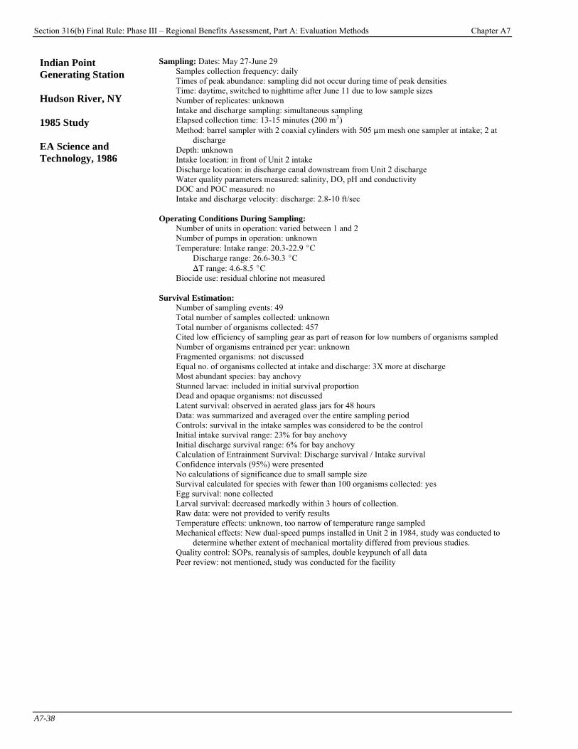
Section 316(b) Final Rule: Phase III – Regional Benefits Assessment, Part A: Evaluation Methods Chapter A7
A7-38
Indian Point Generating Station Hudson River, NY 1985 Study EA Science and Technology, 1986
Sampling: Dates: May 27-June 29 Samples collection frequency: daily Times of peak abundance: sampling did not occur during time of peak densities Time: daytime, switched to nighttime after June 11 due to low sample sizes Number of replicates: unknown Intake and discharge sampling: simultaneous sampling Elapsed collection time: 13-15 minutes (200 mP
3P)
Method: barrel sampler with 2 coaxial cylinders with 505 :m mesh one sampler at intake; 2 at discharge
Depth: unknown Intake location: in front of Unit 2 intake Discharge location: in discharge canal downstream from Unit 2 discharge Water quality parameters measured: salinity, DO, pH and conductivity DOC and POC measured: no Intake and discharge velocity: discharge: 2.8-10 ft/sec
Operating Conditions During Sampling: Number of units in operation: varied between 1 and 2 Number of pumps in operation: unknown Temperature: Intake range: 20.3-22.9 EC
Discharge range: 26.6-30.3 EC )T range: 4.6-8.5 EC
Biocide use: residual chlorine not measured
Survival Estimation: Number of sampling events: 49 Total number of samples collected: unknown Total number of organisms collected: 457 Cited low efficiency of sampling gear as part of reason for low numbers of organisms sampled Number of organisms entrained per year: unknown Fragmented organisms: not discussed Equal no. of organisms collected at intake and discharge: 3X more at discharge Most abundant species: bay anchovy Stunned larvae: included in initial survival proportion Dead and opaque organisms: not discussed Latent survival: observed in aerated glass jars for 48 hours Data: was summarized and averaged over the entire sampling period Controls: survival in the intake samples was considered to be the control Initial intake survival range: 23% for bay anchovy Initial discharge survival range: 6% for bay anchovy Calculation of Entrainment Survival: Discharge survival / Intake survival Confidence intervals (95%) were presented No calculations of significance due to small sample size Survival calculated for species with fewer than 100 organisms collected: yes Egg survival: none collected Larval survival: decreased markedly within 3 hours of collection. Raw data: were not provided to verify results Temperature effects: unknown, too narrow of temperature range sampled Mechanical effects: New dual-speed pumps installed in Unit 2 in 1984, study was conducted to
determine whether extent of mechanical mortality differed from previous studies. Quality control: SOPs, reanalysis of samples, double keypunch of all data Peer review: not mentioned, study was conducted for the facility

Section 316(b) Final Rule: Phase III – Regional Benefits Assessment, Part A: Evaluation Methods Chapter A7
A7-39
Indian Point Generating Station Hudson River, NY 1988 Study EA Engineering, Science, and Technology, 1989
Sampling: Dates: June 8-June 30 Samples collection frequency: unclear Times of peak abundance: sampling not at peak densities for targeted species Time: afternoon and evening hours Number of replicates: varied, unknown number per day Intake and discharge sampling: simultaneous with twice as many at discharge Elapsed collection time: 15 minutes Method: rear-draw sampling flumes, 1 at intake and 2 at discharge Depth: unknown at intake, surface at bottom at discharge Intake location: on raft in front of Intake 35 Discharge location: downstream from flow of Units 2 and 3 Water quality parameters measured: salinity, DO, pH DOC and POC measured: no Intake and discharge velocity: discharge 2.2-10.0 ft/sec
Operating Conditions During Sampling: Number of units in operation: unknown Number of pumps in operation: unknown Temperature: Intake range: 20.3-23.8 EC
)T range: not provided Biocide use: residual chlorine not monitored
Survival Estimation: Number of sampling events: 13 Total number of samples collected: unknown Total number of organisms collected: 12,333 Number of organisms entrained per year: unknown Fragmented organisms: not discussed Equal number of organisms collected at intake and discharge: 10X more in discharge Most abundant species: bay anchovy, striped bass, white perch Stunned larvae: included in initial survival proportion Dead and opaque organisms: not discussed Latent survival: observed in aerated glass jars for 24 hours Data: was summarized and averaged over the entire sampling period; discharge survival
estimates include data from direct release studies and combined surface and bottom samples
Controls: survival in the intake samples was considered to be the control Initial intake survival range: 0-8% for bay anchovy; 86-90% for striped bass Initial discharge survival range: 0-2% for bay anchovy; 62-68% for striped bass Calculation of Entrainment Survival: discharge survival / intake survival Standard errors were presented Significant differences were not tested between the intake and discharge survival Survival calculated for species with fewer than 100 organisms collected: yes Egg survival: none survived in intake and discharge samples Larval survival: decreased markedly within hours of collection Raw data: were not provided to verify results Temperature effects: undetermined effect; too narrow range tested Mechanical effects: study was conducted to determine the effect of the installation of dual speed
circulating water pumps in Unit 2 in 1984 and variable speed pumps in Unit 3 in 1985; mechanical effects were determined to be main cause of mortality when discharge temperatures are <32 EC
Quality control: SOPs, sampling stress evaluation, reanalysis of samples, double keypunch data Peer review: not mentioned, study was conducted for the facility

Section 316(b) Final Rule: Phase III – Regional Benefits Assessment, Part A: Evaluation Methods Chapter A7
A7-40
Indian River Power Plant Indian River Estuary 1975-1976 Study Ecological Analysts, 1978b
Sampling: Dates: July 2, 1975-December 13, 1976 Samples collection frequency: once or twice monthly Times of peak abundance: samples not taken frequently enough to detect Time: mostly at night Number of replicates: varied Intake and discharge sampling: not paired discharge samples not always collected Elapsed collection time: approximately 5 minutes or until sufficient # collected Method: 0.5 m diameter plankton sled with 505 :m net rinsed in 10L of water of unspecified
origin Depth: unknown Intake location: from foot bridge over intake canal Discharge location: in discharge canal under roadway bridge Water quality parameters measured: unknown DOC and POC measured: no Intake and discharge velocity: unknown
Operating Conditions During Sampling: Number of units in operation: unknown Number of pumps in operation: unknown Temperature: Intake range: -0.2-29.2
Discharge range: 5.4-39 EC )T ranged from 5.2-9.0 EC
Biocide use was not noted Survival Estimation:
Number of sampling events: 27 Total number of samples collected: 25 intake and 21 discharge Total number of organisms collected: unknown Number of organisms entrained per year: unknown Fragmented organisms: not discussed Equal number of organisms collected at intake and discharge: unknown Most abundant species: bay anchovy, Atlantic croaker, spot, weakfish, Atlantic menhaden and Atlantic silversides Stunned larvae: not discussed Dead and opaque organisms: not discussed Latent survival: in holding containers in ambient water baths for 96 hours Data: sorted based on discharge temperature Controls: survival in the intake samples was considered to be the control. Initial intake survival range: not provided Initial discharge survival range: not provided Calculation of Entrainment Survival: not all were counted for most abundant species, a random
sample was used instead Confidence intervals / standard deviations: were not presented. Significant differences were not tested between the intake and discharge survival Survival calculated for species with fewer than 100 organisms: unknown Egg survival: were alive in either the intake or discharge samples. Larval survival: unclear trend Raw data: in Appendix B not available to EPA Temperature effects: all species had lower survival at discharge temps >20 °C. Only Spot
survived above 35 EC though linear regression Mechanical effects: unknown, however dye studies performed at this facility and recirculation
of discharge water has been shown to occur. The extent to which organisms are entrained repeatedly and the effect this has on the number of organisms that were shown to have died through natural causes or from sampling is not known. Thus some intake mortality may be due to the organism’s previous passage through the facility.
Quality control: unknown Peer review: not mentioned, study was conducted for the facility

Section 316(b) Final Rule: Phase III – Regional Benefits Assessment, Part A: Evaluation Methods Chapter A7
A7-41
Muskingum River Plant Muskingum River, OH Literature Review Ecological Analysts, 1979a
Sampling: No on site sampling conducted
Operating Conditions During Sampling: No sampling conducted
Survival Estimation:
Analyzed pressure regimes in circulating water system Measured discharge temperature and )T at the facility Determined that pressure regimes were similar to facilities with entrainment survival studies Determined that low survival occurs at )T >7.8 EC which occurs for a small portion of
entrainment season Reviewed documentation of survival at other steam electric stations Concluded that potential of survival at this facility was intermediate to high Peer review: literature review prepared for facility

Section 316(b) Final Rule: Phase III – Regional Benefits Assessment, Part A: Evaluation Methods Chapter A7
A7-42
Northport Generating Station Long Island Sound, NY 1980 Study Ecological Analysts, 1981c
Sampling: Dates: April 10-22 and July 10-23 Samples collection frequency: 5 nights per week Times of peak abundance: attempted to coincide with peak abundance Time: 1700-0100 hours Number of replicates: unknown Intake and discharge sampling: simultaneous Elapsed collection time: 15 minutes Method: floating rear-draw sampling flume with 505 :m mesh screens with ambient water
injection system Depth: intake: 2-8 m below surface; discharge: 1.5 m Intake location: immediately in front of Unit 2 or 3 trash racks Discharge location: immediately in front of Unit 2 or 3 seal well Water quality parameters measured: DO, pH, conductivity DOC and POC measured: no Intake and discharge velocity: unknown
Operating Conditions During Sampling: Number of units in operation: unknown Number of pumps in operation: unknown Temperature: Discharge range: 15.9-35 EC, average 19.9 in April and 33.6 in July
)T ranged from 8.6-15.0 EC Biocide use was not noted
Survival Estimation:
Number of sampling events: 20 Total number of samples collected: 162 Total number of organisms collected: 884 in April and 76 in July Number of organisms entrained per year: unknown Fragmented organisms: not discussed Equal number of organisms collected at intake and discharge: more at discharge Most abundant species: American sand lance, winter flounder, northern pipefish Stunned larvae: included in initial survival proportion Dead and opaque organisms: not discussed Latent survival: observed in aerated jars of filtered ambient water for 48 hours Data: was summarized and averaged over the entire sampling period Controls: survival in the intake samples was considered to be the control Initial intake survival range: 66% for American sand lance; 85% for winter flounder
28% for bay anchovy Initial discharge survival range: 17% for American sand lance; 35% for winter flounder
0% for bay anchovy Calculation of Entrainment Survival: discharge survival / intake survival Stated that survival estimate based on 4 assumptions: that the survival at the discharge is the
product of the probabilities of surviving entrainment and sampling, that the survival at the intake is the probability of surviving sampling, that at the discharge there is no interaction between the two stresses, and each life stage consists of a homogenous population in which all individuals have the same probability of surviving to the next life stage
Standard errors were presented Significant differences were not tested between the intake and discharge survival Survival calculated for species with fewer than 100 organisms collected: yes Egg survival: none collected Larval survival: decreased markedly within 6 hours of collection.
American sand lance significantly larger in intake sample Raw data: were provided to verify results Temperature effects: not studied Mechanical effects: not studied Quality control: SOPs, color coded labels, sorting efficiency checks Peer review: not mentioned, study was conducted for the facility
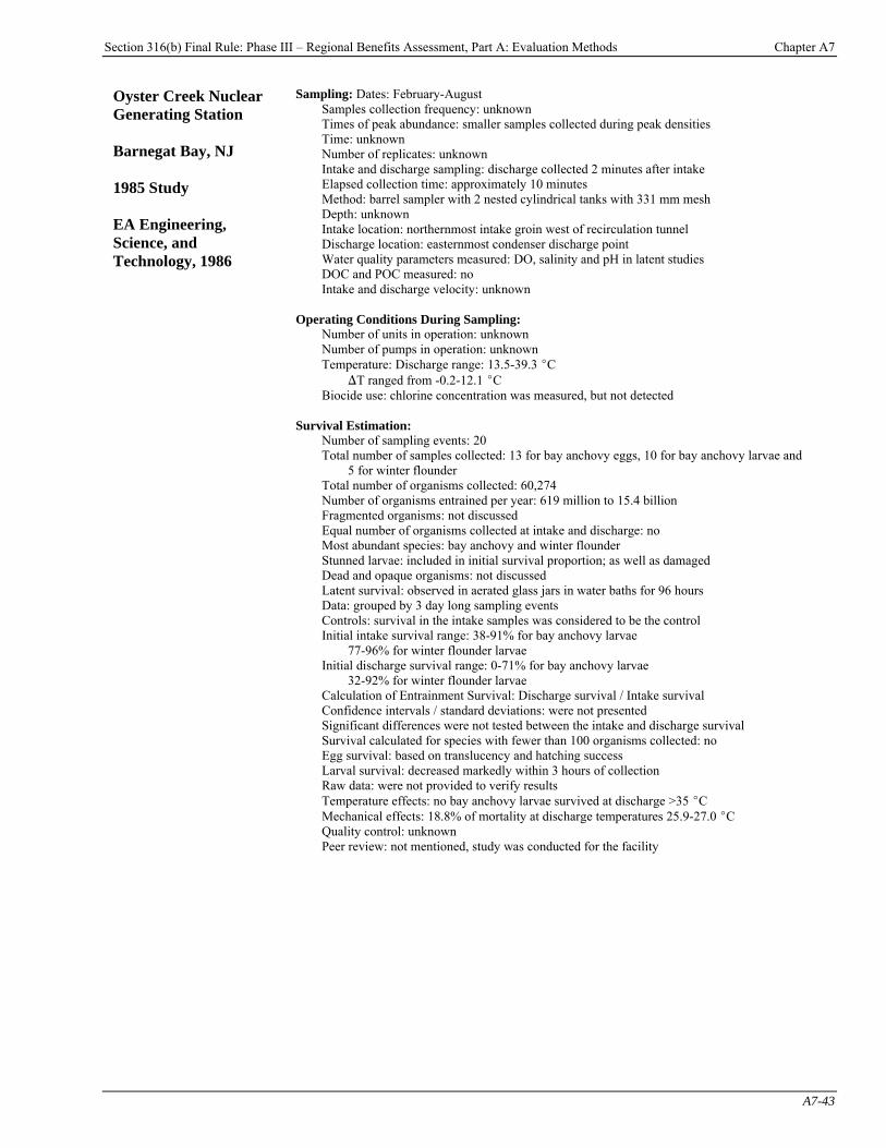
Section 316(b) Final Rule: Phase III – Regional Benefits Assessment, Part A: Evaluation Methods Chapter A7
A7-43
Oyster Creek Nuclear Generating Station Barnegat Bay, NJ 1985 Study EA Engineering, Science, and Technology, 1986
Sampling: Dates: February-August Samples collection frequency: unknown Times of peak abundance: smaller samples collected during peak densities Time: unknown Number of replicates: unknown Intake and discharge sampling: discharge collected 2 minutes after intake Elapsed collection time: approximately 10 minutes Method: barrel sampler with 2 nested cylindrical tanks with 331 mm mesh Depth: unknown Intake location: northernmost intake groin west of recirculation tunnel Discharge location: easternmost condenser discharge point Water quality parameters measured: DO, salinity and pH in latent studies DOC and POC measured: no Intake and discharge velocity: unknown
Operating Conditions During Sampling: Number of units in operation: unknown Number of pumps in operation: unknown Temperature: Discharge range: 13.5-39.3 EC
)T ranged from -0.2-12.1 EC Biocide use: chlorine concentration was measured, but not detected
Survival Estimation: Number of sampling events: 20 Total number of samples collected: 13 for bay anchovy eggs, 10 for bay anchovy larvae and
5 for winter flounder Total number of organisms collected: 60,274 Number of organisms entrained per year: 619 million to 15.4 billion Fragmented organisms: not discussed Equal number of organisms collected at intake and discharge: no Most abundant species: bay anchovy and winter flounder Stunned larvae: included in initial survival proportion; as well as damaged Dead and opaque organisms: not discussed Latent survival: observed in aerated glass jars in water baths for 96 hours Data: grouped by 3 day long sampling events Controls: survival in the intake samples was considered to be the control Initial intake survival range: 38-91% for bay anchovy larvae
77-96% for winter flounder larvae Initial discharge survival range: 0-71% for bay anchovy larvae
32-92% for winter flounder larvae Calculation of Entrainment Survival: Discharge survival / Intake survival Confidence intervals / standard deviations: were not presented Significant differences were not tested between the intake and discharge survival Survival calculated for species with fewer than 100 organisms collected: no Egg survival: based on translucency and hatching success Larval survival: decreased markedly within 3 hours of collection Raw data: were not provided to verify results Temperature effects: no bay anchovy larvae survived at discharge >35 EC Mechanical effects: 18.8% of mortality at discharge temperatures 25.9-27.0 EC Quality control: unknown Peer review: not mentioned, study was conducted for the facility

Section 316(b) Final Rule: Phase III – Regional Benefits Assessment, Part A: Evaluation Methods Chapter A7
A7-44
Pittsburg Power Plant Suisun Bay, CA 1976 Study Stevens and Finlayson, 1978
Sampling: Dates: April 28-July 10 Samples collection frequency: once per week Times of peak abundance: unknown Time: varied, about 25% of all samples collected at night Number of replicates: typically 3 Intake and discharge sampling: paired at closest time and temperature Elapsed collection time: 1-2 minutes Method: 505 micron mech conical nylon plankton net with 0.58 m plastic collecting tubes on
cod end; towed net on boat at 0.6 ft/sec Depth: mid-depth Intake location: in river near intake Discharge location: in river near discharge Water quality parameters measured: none DOC and POC measured: no Intake and discharge velocity: unknown
Operating Conditions During Sampling: Number of units in operation: unknown Number of pumps in operation: unknown Temperature: Intake temperature: 18-30 EC
Discharge temperature 27-37 EC Biocide use was not noted
Survival Estimation: Number of sampling events: 7 Total number of samples collected: unknown Total number of organisms collected: 462 (585 at north shore control) Number of organisms entrained per year: unknown Fragmented organisms: enumerated in one replicate tow higher proportion of unidentifiable
fragments in intake 43% in intake; 19% in discharge
Equal number of organisms collected at intake and discharge: more at intake Most abundant species: striped bass Stunned larvae: included in initial survival proportion Dead and opaque organisms: not discussed Latent survival: not studied Data: was summarized by mean larval length Controls: survival in the intake samples was considered to be the control additional controls in
center of river and north shore control site at north shore away from intake had lower mortality rates
Initial intake survival range: 49-93% for striped bass Initial discharge survival range: 8-87% for striped bass Calculation of Entrainment Survival: paired discharge survival divided by paired intake survival Confidence intervals / standard deviations: were not presented Significant differences were not tested between the intake and discharge survival Survival calculated for species with fewer than 100 organisms collected: yes Egg survival: not studied Larval survival: increased survival with greater larval length Raw data: were not provided to verify results Temperature effects: mortality increased with increase in discharge temperature higher mortality
with discharge temp. >31 and )T >7 EC linear regression showed that half died at temps >33.3 EC 0% survival at temperatures of 38 EC
Mechanical effects: stated not as much of an effects as temperature; recirculated water may be cause of some intake mortality
Quality control: not discussed Peer review: study conducted by California Fish and Game with funds provided by facility
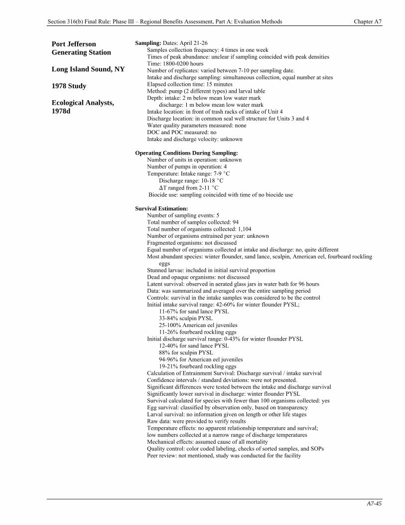
Section 316(b) Final Rule: Phase III – Regional Benefits Assessment, Part A: Evaluation Methods Chapter A7
A7-45
Port Jefferson Generating Station Long Island Sound, NY 1978 Study Ecological Analysts, 1978d
Sampling: Dates: April 21-26 Samples collection frequency: 4 times in one week Times of peak abundance: unclear if sampling coincided with peak densities Time: 1800-0200 hours Number of replicates: varied between 7-10 per sampling date. Intake and discharge sampling: simultaneous collection, equal number at sites Elapsed collection time: 15 minutes Method: pump (2 different types) and larval table Depth: intake: 2 m below mean low water mark
discharge: 1 m below mean low water mark Intake location: in front of trash racks of intake of Unit 4 Discharge location: in common seal well structure for Units 3 and 4 Water quality parameters measured: none DOC and POC measured: no Intake and discharge velocity: unknown
Operating Conditions During Sampling: Number of units in operation: unknown Number of pumps in operation: 4 Temperature: Intake range: 7-9 EC
Discharge range: 10-18 EC )T ranged from 2-11 EC
Biocide use: sampling coincided with time of no biocide use
Survival Estimation: Number of sampling events: 5 Total number of samples collected: 94 Total number of organisms collected: 1,104 Number of organisms entrained per year: unknown Fragmented organisms: not discussed Equal number of organisms collected at intake and discharge: no, quite different Most abundant species: winter flounder, sand lance, sculpin, American eel, fourbeard rockling
eggs Stunned larvae: included in initial survival proportion Dead and opaque organisms: not discussed Latent survival: observed in aerated glass jars in water bath for 96 hours Data: was summarized and averaged over the entire sampling period Controls: survival in the intake samples was considered to be the control Initial intake survival range: 42-60% for winter flounder PYSL;
11-67% for sand lance PYSL 33-84% sculpin PYSL 25-100% American eel juveniles 11-26% fourbeard rockling eggs
Initial discharge survival range: 0-43% for winter flounder PYSL 12-40% for sand lance PYSL 88% for sculpin PYSL 94-96% for American eel juveniles 19-21% fourbeard rockling eggs
Calculation of Entrainment Survival: Discharge survival / intake survival Confidence intervals / standard deviations: were not presented. Significant differences were tested between the intake and discharge survival Significantly lower survival in discharge: winter flounder PYSL Survival calculated for species with fewer than 100 organisms collected: yes Egg survival: classified by observation only, based on transparency Larval survival: no information given on length or other life stages Raw data: were provided to verify results Temperature effects: no apparent relationship temperature and survival; low numbers collected at a narrow range of discharge temperatures Mechanical effects: assumed cause of all mortality Quality control: color coded labeling, checks of sorted samples, and SOPs Peer review: not mentioned, study was conducted for the facility

Section 316(b) Final Rule: Phase III – Regional Benefits Assessment, Part A: Evaluation Methods Chapter A7
A7-46
PG&E Potrero Power Plant San Francisco Bay, CA 1979 Study Ecological Analysts, 1980b
Sampling: Dates: January Samples collection frequency: unknown Times of peak abundance: unclear if sampling corresponded with peak densities Time: unknown Number of replicates: unknown Intake and discharge sampling: equal number but timing unknown Elapsed collection time: 15 minutes Method: 2 pumps and larval table with filtered ambient temperature water flow Depth: mid-depth Intake location: directly in front of intake skimmer wall Discharge location: at point where discharge enters San Francisco Bay Water quality parameters measured: none DOC and POC measured: no Intake and discharge velocity: unknown
Operating Conditions During Sampling: Number of units in operation: unknown Number of pumps in operation: unknown Temperature: Discharge range: 18-19.5 EC
)T range not presented Biocide use: not used during sampling events
Survival Estimation: Number of sampling events: 11 Total number of samples collected: 25 Total number of organisms collected: 1,262 Number of organisms entrained per year: estimated for Units 1-3: 3 billion Fragmented organisms: not discussed Equal number of organisms collected at intake and discharge: approx. same Most abundant species: Pacific herring Stunned larvae: issue of stunned larvae not discussed in study Dead and opaque organisms: not discussed Latent survival: observed in aerated glass jars in water baths for 96 hours Data: was summarized and averaged over the entire sampling period Controls: survival in the intake samples was considered to be the control Initial intake survival range: 22% for Pacific herring Initial discharge survival range: 16% for Pacific herring Calculation of Entrainment Survival: Discharge survival/ Intake survival Confidence intervals / standard deviations: were not presented. Significant differences were not tested between the intake and discharge survival Survival calculated for species with fewer than 100 organisms collected: no Egg survival: not studied Larval survival: Based on results of this study, an estimate of 75% entrainment survival was
used for all species and life stages entrained at this facility under all conditions Raw data: were not provided to verify results Temperature effects: discharge temps <30 EC over 99.5% of time Mechanical effects: most likely cause of mortality due to low temperatures Quality control: unknown Peer review: not mentioned, study was conducted for the facility
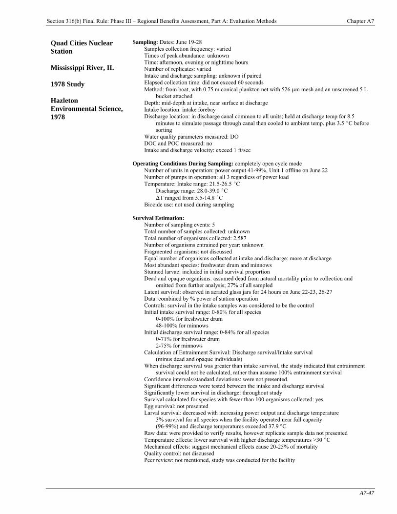
Section 316(b) Final Rule: Phase III – Regional Benefits Assessment, Part A: Evaluation Methods Chapter A7
A7-47
Quad Cities Nuclear Station Mississippi River, IL 1978 Study Hazleton Environmental Science, 1978
Sampling: Dates: June 19-28 Samples collection frequency: varied Times of peak abundance: unknown Time: afternoon, evening or nighttime hours Number of replicates: varied Intake and discharge sampling: unknown if paired Elapsed collection time: did not exceed 60 seconds Method: from boat, with 0.75 m conical plankton net with 526 :m mesh and an unscreened 5 L
bucket attached Depth: mid-depth at intake, near surface at discharge Intake location: intake forebay Discharge location: in discharge canal common to all units; held at discharge temp for 8.5
minutes to simulate passage through canal then cooled to ambient temp. plus 3.5 EC before sorting
Water quality parameters measured: DO DOC and POC measured: no Intake and discharge velocity: exceed 1 ft/sec
Operating Conditions During Sampling: completely open cycle mode Number of units in operation: power output 41-99%, Unit 1 offline on June 22 Number of pumps in operation: all 3 regardless of power load Temperature: Intake range: 21.5-26.5 EC
Discharge range: 28.0-39.0 EC )T ranged from 5.5-14.8 EC
Biocide use: not used during sampling
Survival Estimation: Number of sampling events: 5 Total number of samples collected: unknown Total number of organisms collected: 2,587 Number of organisms entrained per year: unknown Fragmented organisms: not discussed Equal number of organisms collected at intake and discharge: more at discharge Most abundant species: freshwater drum and minnows Stunned larvae: included in initial survival proportion Dead and opaque organisms: assumed dead from natural mortality prior to collection and
omitted from further analysis; 27% of all sampled Latent survival: observed in aerated glass jars for 24 hours on June 22-23, 26-27 Data: combined by % power of station operation Controls: survival in the intake samples was considered to be the control Initial intake survival range: 0-80% for all species
0-100% for freshwater drum 48-100% for minnows
Initial discharge survival range: 0-84% for all species 0-71% for freshwater drum 2-75% for minnows
Calculation of Entrainment Survival: Discharge survival/Intake survival (minus dead and opaque individuals)
When discharge survival was greater than intake survival, the study indicated that entrainment survival could not be calculated, rather than assume 100% entrainment survival
Confidence intervals/standard deviations: were not presented. Significant differences were tested between the intake and discharge survival Significantly lower survival in discharge: throughout study Survival calculated for species with fewer than 100 organisms collected: yes Egg survival: not presented Larval survival: decreased with increasing power output and discharge temperature
3% survival for all species when the facility operated near full capacity (96-99%) and discharge temperatures exceeded 37.9 °C
Raw data: were provided to verify results, however replicate sample data not presented Temperature effects: lower survival with higher discharge temperatures >30 EC Mechanical effects: suggest mechanical effects cause 20-25% of mortality Quality control: not discussed Peer review: not mentioned, study was conducted for the facility
Section 316(b) Final Rule: Phase III – Regional Benefits Assessment, Part A: Evaluation Methods Chapter A7
A7-48
Quad Cities Nuclear Station Mississippi River, IL 1984 Study Lawler, Matusky & Skelly Engineers, 1985
Sampling: Dates: April 25-June 27 July sampling canceled as 100% mortality was suspected Samples collection frequency: weekly Times of peak abundance: unknown Time: unknown Number of replicates: unknown Intake and discharge sampling: unknown if paired Elapsed collection time: unknown Method: from boat, with 0.75 m conical plankton net with 526 :m mesh and an unscreened 5 L
bucket attached Depth: 1.5 m for intake, surface for discharge Intake location: intake forebay Discharge location: in discharge canal; held at collection temperature for 8.5 min. then cooled to
3.5 EC above ambient temperature with an ice bath, in all held for over 20 minutes before sorting
Water quality parameters measured: none DOC and POC measured: no Intake and discharge velocity: samples collected at <0.8 ft/sec
Operating Conditions During Sampling: operating at 40.2 to 50.7% capacity Number of units in operation: Unit 1 offline for refueling;
both units offline on May 9 Number of pumps in operation: all 3 on all dates except on May 9 Temperature: Intake range: 11-24.4 EC
Discharge range: 12-37 EC )T ranged from 9.5 to 14.5 EC; 1 EC on May 9 when offline
Biocide use: not used during sampling
Survival Estimation: Number of sampling events: 8 Total number of samples collected: unknown Total number of organisms collected: 3,967 Number of organisms entrained per year: unknown Fragmented organisms: not discussed Equal number of organisms collected at intake and discharge: approx. same total Most abundant species: freshwater drum, carp and buffalo Stunned larvae: not discussed Dead and opaque organisms: omitted from analysis; assumed dead before collection, 2,979
opaque individuals were collected (75% of total, 87% of all discharge sample. range: 0 to 99% in samples) None were found to be dead and opaque in discharge on May 9 when offline and )T was 1° C.
Latent survival: not discussed Data: combined by species and sampling date Controls: survival in the intake samples was considered to be the control Initial intake survival range: results not presented, only number alive
10-81% were dead and opaque Initial discharge survival range: results not presented, only number alive
24-99% were dead and opaque Calculation of Entrainment Survival: Discharge survival / Intake survival Confidence intervals / standard deviations: were not presented. Significant differences were not tested due to low numbers collected Survival calculated for species with fewer than 100 organisms collected: yes Egg survival: not studied Larval survival: too little information to make any assumption of survival Raw data: were not provided to verify results; totals collected per species not presented; actual
numbers of dead and opaque not provided Temperature effects: no sampling in July when discharge temps >37 EC Mechanical effects: not discussed Quality control: 100% reanalysis quality control Peer review: not mentioned, study was conducted for the facility

Section 316(b) Final Rule: Phase III – Regional Benefits Assessment, Part A: Evaluation Methods Chapter A7
A7-49
Roseton Generating Station Hudson River, NY 1975 Study Ecological Analysts, 1976c
Sampling: Dates: May 29P
thP-November 18P
thP
Collection frequency: varied from 4 times per week to once every 2 weeks. Times of peak abundance: greater frequency of collection Time: varied but generally occurred between dusk and dawn Number of replicates: varied between 3 and 14 for each date Intake and discharge sampling: paired but timing not standardized Elapsed collection time: not noted Method: pump/larval table Depth: mid-depth at both the intake and discharge Intake location: in front of the trash rack Discharge location: from the seal well before the end of the discharge pipe Water quality parameters measured: none mentioned DOC and POC measured: no Intake and discharge velocity: not given
Operating Conditions During Sampling: Number of units in operation: varied between 1 and 2 Number of pumps in operation: varied between 2 and 3 Temperature: )T ranged from 3 to 13 EC, intake and discharge T not given Biocide use: not noted
Survival Estimation: Number of sampling events: 41 Number of samples: 672 Number of organisms collected: 3,667 Number of organisms entrained per year: not discussed Fragmented organisms collected: not discussed Equal number collected from intake and discharge: differed by as much as 3.2X Most abundant species: striped bass, white perch, alewife and blueback herring Stunned larvae: included in initial survival proportion Dead and opaque organisms: not mentioned Latent survival: observed in aerated glass jars for 96 hours. Data: summarized and averaged over the entire sampling period Controls: survival in intake sample; no other control Initial intake survival range: 57 to 80% for striped bass
0 to 71% for white perch 58 to 65% for herrings
Initial discharge survival range: 62% for striped bass 29% for white perch 26% for herrings
Calculation of entrainment survival: Discharge Survival/Intake Survival Study noted that survival cannot be calculated with insufficient data or when intake survival is
very low Confidence intervals/ standard deviations: not presented Significant differences: tested between the intake and discharge survival Significantly lower survival in discharge: striped bass YSL and PYSL
white perch PYSL herring PYSL and juveniles
Survival calculated for species with fewer than 100 organisms collected: yes Egg survival: none alive in either the intake or discharge samples Larval survival: decreased markedly within 3 hours of collection Size effects: survival by larval length was not studied Raw data: were not provided to verify results Temperature effects: not provided Mechanical effects: not provided Quality control: double check after initial sorting; monitoring of data entry Peer review: not mentioned; study was conducted for the facility
Section 316(b) Final Rule: Phase III – Regional Benefits Assessment, Part A: Evaluation Methods Chapter A7
A7-50
Roseton Generating Station Hudson River, NY 1976 Study Ecological Analysts, 1978e
Sampling: Dates: June 14th-July 30th Samples collection frequency: 4 nights per week Times of peak abundance: coincided with Morone spp. spawning season Time: 1700 to 0300 EST Number of replicates: actual numbers not give, an average of 12 per night stated Intake and discharge sampling: pairing unknown Elapsed collection time: 15 minutes Method: pump/ larval table combination Depth: mid-depth for both intake and discharge Intake location: 1 m in front of trash rack Discharge location: in seal well near end of discharge pipe Water quality parameters measured: no DOC and POC measured: no Intake and discharge velocity: unknown
Operating Conditions During Sampling: Number of units in operation: varied between 0 and 2 Number of pumps in operation: not given Temperature: Intake temperature range: 18.7-27.5 EC
Discharge temperature ranged 24-37 EC )T ranged from 1-10 EC
Biocide use: not noted
Survival Estimation: Number of sampling events: 27 Total number of samples collected: unknown Total number of organisms collected: 3,491 Number of organisms entrained per year: not given Fragmented organisms: not discussed Equal number of organisms collected at intake / discharge: no, up to 5.7X more Most abundant species: herrings, white perch and striped bass Stunned larvae: were included in initial survival proportion Dead and opaque organisms: not mentioned Latent survival: observed in aerated glass jars for 96 hours Data: combined by discharge temperature range: 34-30.5 and 30.6 to 37 EC Controls: Survival in the intake samples; no other control. Initial intake survival range: 74-100% for striped bass
53-94% for white perch 49-68% for herrings
Initial discharge survival range: 14-80% for striped bass 6-56% for white perch 5-29% for herrings
Calculation of Entrainment Survival: Discharge Survival/ Intake Survival Data for many taxa or life stages collected were insufficient for analysis Confidence intervals / standard deviations: were not presented Significant differences were tested between the intake and discharge survival Significantly lower survival in discharge: striped bass PYSL
white perch PYSL and juveniles herring PYSL and juveniles
Survival calculated for species with fewer than 100 organisms collected: yes Egg survival: data not presented Larval survival: decreased markedly within 3 hours of collection. Size effects: survival by larval length was not studied Raw data: were not provided to verify results Temperature effects: significant decrease in survival at discharge temp >30 EC Mechanical effects: unknown Quality control: double check after initial sorting; monitoring of data entry Peer review: not mentioned, study was conducted for the facility
Section 316(b) Final Rule: Phase III – Regional Benefits Assessment, Part A: Evaluation Methods Chapter A7
A7-51
Roseton Generating Station Hudson River, NY 1977 Study Ecological Analysts, 1978f
Sampling: Dates: March 3-17 and May 31P
stP-July 15P
thP
Samples collection frequency: unknown; usually 4 nights per week was stated Times of peak abundance: coincided with spawning of targeted species Time: 1700 to 0300 hours EST Number of replicates: unknown; an average of 8 to 10 per night was stated Intake and discharge sampling: unknown if samples were collected in pairs Elapsed collection time: 15 minutes Method: pump/larval table combination
ambient water flow in table to reduce thermal exposure during sorting Depth: mid-depth Intake location: in front of trash racks Discharge location: from seal well 244 m from end of discharge pipe Water quality parameters measured: no DOC and POC measured: no Intake and discharge velocity: unknown
Operating Conditions During Sampling: Number of units in operation: unknown Number of pumps in operation: varied between 2 and 4 Temperature: Intake temperature: 0.5-5.5 EC (March); 11-27 EC (June/July)
Discharge temperature: 7-17 EC (March); 24-36 EC (June/July) )T range: unknown
Biocide use was not noted
Survival Estimation: Number of sampling events: unknown Total number of samples collected: unknown Total number of organisms collected: 6,973 Number of organisms entrained per year: unknown Fragmented organisms: if >50% present, organism was counted Equal number collected at intake and discharge: up to 2.3X more in discharge Most abundant species: atlantic tomcod, herrings, striped bass, white perch Stunned larvae: included in initial survival proportion Dead and opaque organisms: not mentioned Latent survival: observed in aerated glass jars for 96 hours Data: combined by discharge temperature range, <29.9, 30.0-32.9, >33 EC Controls: Survival in the intake samples was considered to be the control Initial intake survival range: 39% for Atlantic tomcod
0 to 50% for striped bass 0 to 33% for white perch 0 to 59% for herrings
Initial discharge survival range: 16% for Atlantic tomcod 0 to 83% for striped bass 0 to 50% for white perch 0 to 14% for herrings
Calculation of Entrainment Survival: Discharge Survival / Intake Survival Confidence intervals / standard deviations: were not presented. Significant differences were tested between the intake and discharge survival Significantly lower survival in discharge: Atlantic tomcod YSL
striped bass PYSL white perch PYSL herring PYSL and juveniles
Survival calculated for species with fewer than 100 organisms collected: yes number of some taxa and life stage were too low to estimate survival reliably
Egg survival: data not presented Larval survival: decreased markedly within 3 hours of collection.
increased with larval length Raw data: were not provided to verify results Temperature effects: survival decreased at temperatures above 30 EC
very low survival at temperatures >33 EC (0 to 3%) Mechanical effects: survival may increase with number of pumps operating Quality control: color coded labels, immediate checks of sorted sample, SOP’s Peer review: not mentioned, study was conducted for the facility
Section 316(b) Final Rule: Phase III – Regional Benefits Assessment, Part A: Evaluation Methods Chapter A7
A7-52
Roseton Generating Station Hudson River, NY 1978 Study Ecological Analysts, 1980c
Sampling: Dates: March 13-23 and June 6-July 13 Samples collection frequency: 3-4 nights per week Times of peak abundance: coincided with spawning of targeted species Time: 1700 to 0300 EDT Number of replicates: 4 to 10 per night Intake and discharge sampling: unknown if paired samples Elapsed collection time: 15 minutes Method: pump/ larval table combination with fine mesh
ambient water flow to table to minimize thermal exposure when sorting Depth: mid-depth Intake location: in front of trash rack Discharge location: in seal well 244 m from end of discharge pipe Water quality parameters measured: none DOC and POC measured: no Intake and discharge velocity: unknown
Operating Conditions During Sampling: Number of units in operation: varied between 1 and 2 Number of pumps in operation: varied between 2 and 3 Temperature: Intake temperature: 0.2-5.5 EC (March), 19.8-24.0 EC (June/July)
Discharge temperature: 10-19 EC (March), 24-37 EC (June/July) )T range was not given
Biocide use was not noted
Survival Estimation: Number of sampling events: 30 Total number of samples collected: 256 Total number of organisms collected: 5,308 Number of organisms entrained per year: unknown Fragmented organisms: counted if >50% of organism was present
22% of Atlantic tomcod could not be identified to life stage due to damage Equal number of organisms collected at intake and discharge: varied Most abundant species: herrings, white perch, striped bass, Atlantic tomcod Stunned larvae: included in initial survival proportion Dead and opaque organisms: not mentioned Latent survival: observed in aerated glass jars for 96 hours Data: combined by discharge temperature range <29.9, 30.0-32.9, >33 EC
also combined by larval length Controls: Survival in the intake samples was considered to be the control Initial intake survival range: 75-84% for Atlantic tomcod
8-100% for striped bass 0-93% for white perch 0-67% for herrings
Initial discharge survival range: 23-33% for Atlantic tomcod 0-50% for striped bass 0-100% for white perch 0-18% for herrings
Calculation of Entrainment Survival: Discharge survival/ Intake survival Confidence intervals/standard deviations: were not presented Significant differences were tested between the intake and discharge survival Significantly lower survival in discharge: Atlantic tomcod YSL and PYSL
striped bass PYSL white perch PYSL herring PYSL
Survival calculated for species with fewer than 100 organisms collected: yes samples sizes of some taxa and life stages were too small to analyze survival
Egg survival: data not presented Larval survival: decreased markedly within 3-6 hours of collection
increased with larval length Raw data: consolidated data by temp. and length was provided; not by sample Temperature effects: significant decrease in survival at temperatures >24 EC
very little survival at temperatures >30 EC Mechanical effects: lower tomcod survival in discharge w/o thermal effects Quality control: color coded labels, checks of sorted samples, SOP’s Peer review: not mentioned, study was conducted for the facility
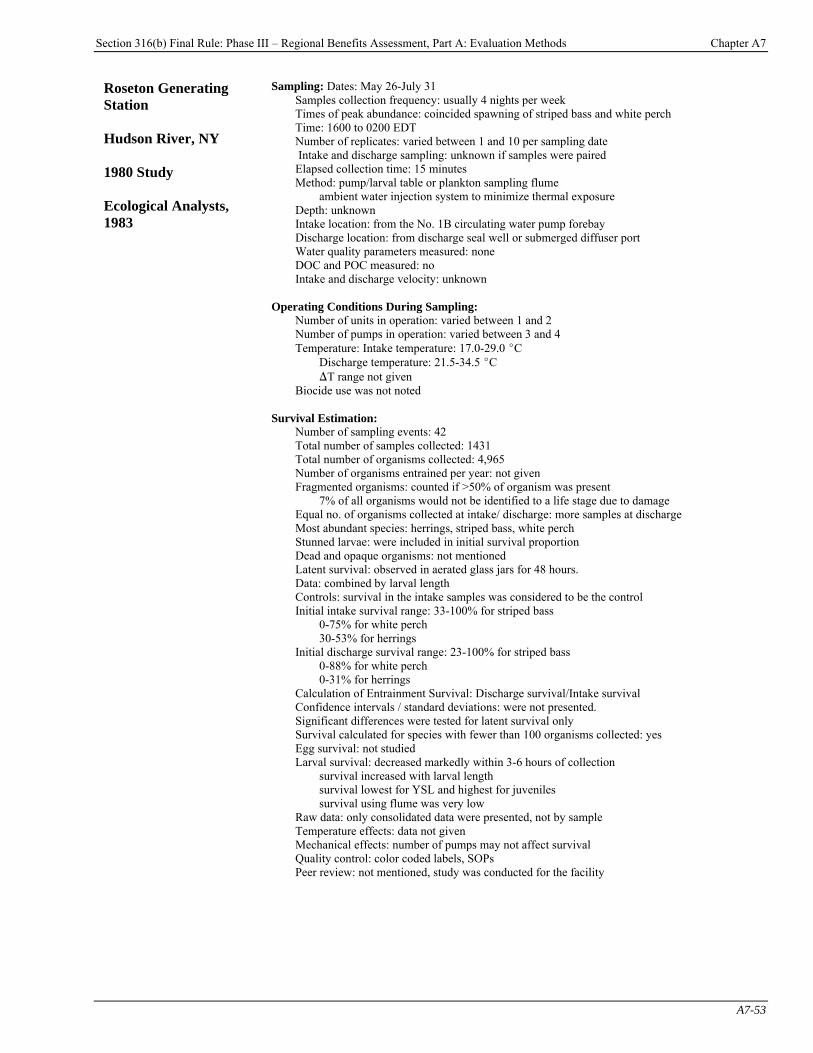
Section 316(b) Final Rule: Phase III – Regional Benefits Assessment, Part A: Evaluation Methods Chapter A7
A7-53
Roseton Generating Station Hudson River, NY 1980 Study Ecological Analysts, 1983
Sampling: Dates: May 26-July 31 Samples collection frequency: usually 4 nights per week Times of peak abundance: coincided spawning of striped bass and white perch Time: 1600 to 0200 EDT Number of replicates: varied between 1 and 10 per sampling date Intake and discharge sampling: unknown if samples were paired Elapsed collection time: 15 minutes Method: pump/larval table or plankton sampling flume
ambient water injection system to minimize thermal exposure Depth: unknown Intake location: from the No. 1B circulating water pump forebay Discharge location: from discharge seal well or submerged diffuser port Water quality parameters measured: none DOC and POC measured: no Intake and discharge velocity: unknown
Operating Conditions During Sampling: Number of units in operation: varied between 1 and 2 Number of pumps in operation: varied between 3 and 4 Temperature: Intake temperature: 17.0-29.0 EC
Discharge temperature: 21.5-34.5 EC )T range not given
Biocide use was not noted Survival Estimation:
Number of sampling events: 42 Total number of samples collected: 1431 Total number of organisms collected: 4,965 Number of organisms entrained per year: not given Fragmented organisms: counted if >50% of organism was present
7% of all organisms would not be identified to a life stage due to damage Equal no. of organisms collected at intake/ discharge: more samples at discharge Most abundant species: herrings, striped bass, white perch Stunned larvae: were included in initial survival proportion Dead and opaque organisms: not mentioned Latent survival: observed in aerated glass jars for 48 hours. Data: combined by larval length Controls: survival in the intake samples was considered to be the control Initial intake survival range: 33-100% for striped bass
0-75% for white perch 30-53% for herrings
Initial discharge survival range: 23-100% for striped bass 0-88% for white perch 0-31% for herrings
Calculation of Entrainment Survival: Discharge survival/Intake survival Confidence intervals / standard deviations: were not presented. Significant differences were tested for latent survival only Survival calculated for species with fewer than 100 organisms collected: yes Egg survival: not studied Larval survival: decreased markedly within 3-6 hours of collection
survival increased with larval length survival lowest for YSL and highest for juveniles survival using flume was very low
Raw data: only consolidated data were presented, not by sample Temperature effects: data not given Mechanical effects: number of pumps may not affect survival Quality control: color coded labels, SOPs Peer review: not mentioned, study was conducted for the facility
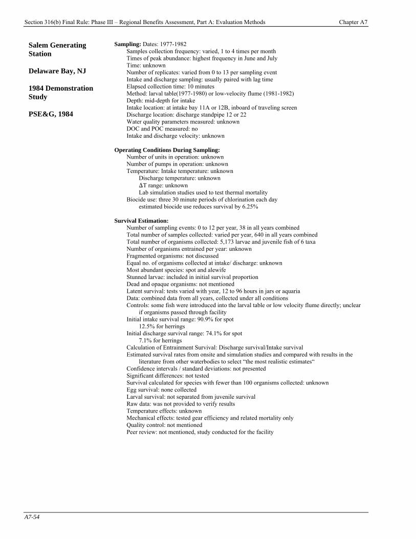
Section 316(b) Final Rule: Phase III – Regional Benefits Assessment, Part A: Evaluation Methods Chapter A7
A7-54
Salem Generating Station Delaware Bay, NJ 1984 Demonstration Study PSE&G, 1984
Sampling: Dates: 1977-1982 Samples collection frequency: varied, 1 to 4 times per month Times of peak abundance: highest frequency in June and July Time: unknown Number of replicates: varied from 0 to 13 per sampling event Intake and discharge sampling: usually paired with lag time Elapsed collection time: 10 minutes Method: larval table(1977-1980) or low-velocity flume (1981-1982) Depth: mid-depth for intake Intake location: at intake bay 11A or 12B, inboard of traveling screen Discharge location: discharge standpipe 12 or 22 Water quality parameters measured: unknown DOC and POC measured: no Intake and discharge velocity: unknown
Operating Conditions During Sampling: Number of units in operation: unknown Number of pumps in operation: unknown Temperature: Intake temperature: unknown
Discharge temperature: unknown )T range: unknown Lab simulation studies used to test thermal mortality
Biocide use: three 30 minute periods of chlorination each day estimated biocide use reduces survival by 6.25%
Survival Estimation:
Number of sampling events: 0 to 12 per year, 38 in all years combined Total number of samples collected: varied per year, 640 in all years combined Total number of organisms collected: 5,173 larvae and juvenile fish of 6 taxa Number of organisms entrained per year: unknown Fragmented organisms: not discussed Equal no. of organisms collected at intake/ discharge: unknown Most abundant species: spot and alewife Stunned larvae: included in initial survival proportion Dead and opaque organisms: not mentioned Latent survival: tests varied with year, 12 to 96 hours in jars or aquaria Data: combined data from all years, collected under all conditions Controls: some fish were introduced into the larval table or low velocity flume directly; unclear
if organisms passed through facility Initial intake survival range: 90.9% for spot
12.5% for herrings Initial discharge survival range: 74.1% for spot
7.1% for herrings Calculation of Entrainment Survival: Discharge survival/Intake survival Estimated survival rates from onsite and simulation studies and compared with results in the
literature from other waterbodies to select “the most realistic estimates“ Confidence intervals / standard deviations: not presented Significant differences: not tested Survival calculated for species with fewer than 100 organisms collected: unknown Egg survival: none collected Larval survival: not separated from juvenile survival Raw data: was not provided to verify results Temperature effects: unknown Mechanical effects: tested gear efficiency and related mortality only Quality control: not mentioned Peer review: not mentioned, study conducted for the facility

Section 316(b) Final Rule: Phase III – Regional Benefits Assessment, Part A: Evaluation Methods Chapter A8
A8-1
Chapter A8: Discounting Benefits Introduction Discounting refers to the economic conversion of future benefits and costs to their present values, accounting for the fact that individuals tend to value future outcomes less than comparable near-term outcomes. Annualization refers to the conversion of a series of annual costs or benefits of differing amounts to an equivalent annual series of constant costs or benefits. Discounting and annualization are important because these techniques allow the comparison of benefits and costs that occur in different time periods.
Chapter Contents A8-1 Timing of Benefits ..................................... A8-1 A8-2 Discounting and Annualization.................. A8-2
For the benefits analysis of the regulatory analysis options for the final section 316(b) regulation for Phase III facilities, EPA’s discounting and annualization methodology included three steps. First, EPA developed a time profile of benefits to show when benefits occur. Second, the Agency calculated the total discounted value of the benefits as of the year 2007. Finally, EPA annualized the benefits of the regulatory analysis options over a thirty-year time span. The following sections explain these steps in detail. A8-1 Timing of Benefits In order to calculate the annualized value of the welfare gain from the regulatory analysis options considered for the final section 316(b) regulation for Phase III facilities, EPA developed a time profile of total benefits from all Phase III facilities that reflects when benefits from each facility will be realized. EPA first calculated the undiscounted commercial and recreational welfare gain from the expected annual regional reductions in impingement and entrainment (I&E) under each analysis option, based on the assumptions that all facilities in each region have achieved compliance with each respective option and that benefits are realized immediately following compliance. Then, since there are regulatory and biological time lags between the potential promulgation of each respective analysis option and the realization of benefits, EPA created a time profile of benefits that takes into account the fact that benefits do not begin immediately. Since this time profile requires information about facility-specific differences in magnitude and timing of benefits, but benefits were estimated only on a regional basis, EPA approximated benefits from each facility by multiplying total undiscounted regional benefits by the percentage of total regional flow that is attributable to each facility. Regulatory-related time lags occur because, although the regulatory analysis options take effect at the beginning of 2007, facilities would not need to come into compliance with each respective option until their current NPDES permits expire.PF
1FP EPA used facility-specific permitting information to estimate the lag between the potential
promulgation of the regulatory analysis options and the compliance year for each sample facility. The terms of each facility’s permit differ, but permits for all Phase III facilities are expected to expire between 2010 and 2014. Thus, EPA estimates that it would take from three to seven years after promulgation of each respective analysis option for Phase III facilities to install technologies to reduce I&E. The biological time lags that affect the timing of benefits occur because most fish that would be spared from I&E would be in larval or juvenile stages. Since these fish may require several years to grow and mature before commercial and recreational anglers can harvest them, there would be a lag between installation of technologies
P
1P The final regulation for Phase III facilities is scheduled to be promulgated in June of 2006. However, to simplify
the discounting and annualization calculations for the benefit cost analysis of the regulatory analysis options, EPA assumed that the regulation will take effect on January 1, 2007.
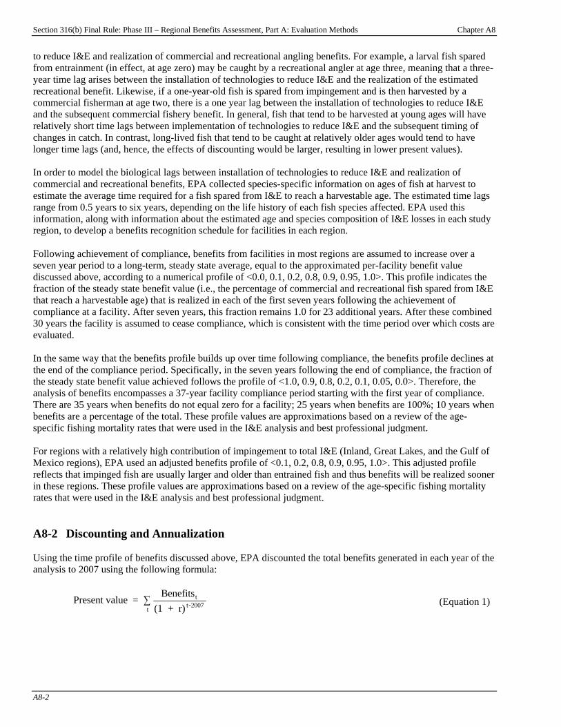
Section 316(b) Final Rule: Phase III – Regional Benefits Assessment, Part A: Evaluation Methods Chapter A8
A8-2
to reduce I&E and realization of commercial and recreational angling benefits. For example, a larval fish spared from entrainment (in effect, at age zero) may be caught by a recreational angler at age three, meaning that a three-year time lag arises between the installation of technologies to reduce I&E and the realization of the estimated recreational benefit. Likewise, if a one-year-old fish is spared from impingement and is then harvested by a commercial fisherman at age two, there is a one year lag between the installation of technologies to reduce I&E and the subsequent commercial fishery benefit. In general, fish that tend to be harvested at young ages will have relatively short time lags between implementation of technologies to reduce I&E and the subsequent timing of changes in catch. In contrast, long-lived fish that tend to be caught at relatively older ages would tend to have longer time lags (and, hence, the effects of discounting would be larger, resulting in lower present values). In order to model the biological lags between installation of technologies to reduce I&E and realization of commercial and recreational benefits, EPA collected species-specific information on ages of fish at harvest to estimate the average time required for a fish spared from I&E to reach a harvestable age. The estimated time lags range from 0.5 years to six years, depending on the life history of each fish species affected. EPA used this information, along with information about the estimated age and species composition of I&E losses in each study region, to develop a benefits recognition schedule for facilities in each region. Following achievement of compliance, benefits from facilities in most regions are assumed to increase over a seven year period to a long-term, steady state average, equal to the approximated per-facility benefit value discussed above, according to a numerical profile of <0.0, 0.1, 0.2, 0.8, 0.9, 0.95, 1.0>. This profile indicates the fraction of the steady state benefit value (i.e., the percentage of commercial and recreational fish spared from I&E that reach a harvestable age) that is realized in each of the first seven years following the achievement of compliance at a facility. After seven years, this fraction remains 1.0 for 23 additional years. After these combined 30 years the facility is assumed to cease compliance, which is consistent with the time period over which costs are evaluated. In the same way that the benefits profile builds up over time following compliance, the benefits profile declines at the end of the compliance period. Specifically, in the seven years following the end of compliance, the fraction of the steady state benefit value achieved follows the profile of <1.0, 0.9, 0.8, 0.2, 0.1, 0.05, 0.0>. Therefore, the analysis of benefits encompasses a 37-year facility compliance period starting with the first year of compliance. There are 35 years when benefits do not equal zero for a facility; 25 years when benefits are 100%; 10 years when benefits are a percentage of the total. These profile values are approximations based on a review of the age-specific fishing mortality rates that were used in the I&E analysis and best professional judgment. For regions with a relatively high contribution of impingement to total I&E (Inland, Great Lakes, and the Gulf of Mexico regions), EPA used an adjusted benefits profile of <0.1, 0.2, 0.8, 0.9, 0.95, 1.0>. This adjusted profile reflects that impinged fish are usually larger and older than entrained fish and thus benefits will be realized sooner in these regions. These profile values are approximations based on a review of the age-specific fishing mortality rates that were used in the I&E analysis and best professional judgment. A8-2 Discounting and Annualization Using the time profile of benefits discussed above, EPA discounted the total benefits generated in each year of the analysis to 2007 using the following formula:
Present value = Benefits(1 + r)
tt-2007
t∑ (Equation 1)

Section 316(b) Final Rule: Phase III – Regional Benefits Assessment, Part A: Evaluation Methods Chapter A8
A8-3
where:
BenefitsBtB = benefits in year t r = discount rate (3% and 7%) t = year in which benefits are incurred (2007 to 2043)
After calculating the present value (PV) of these benefits streams, EPA calculated their constant annual equivalent value (annualized value) using the annualization formula presented below, again using two discount rates, 3% and 7%.TPF
2FPT Although the analysis period extends from 2007 through 2048, a compliance period of 42 years for all
facilities, EPA annualized benefits over 30 years, since 30 years is the assumed period of compliance. This same annualization concept and period of annualization were also followed in the analysis of costs, although for costs the time horizon of analysis for calculating the present value is shorter than for benefits. Using a 30-year annualization period for both benefits and social costs allows comparison of constant annual equivalent values of benefits and costs that have been calculated on a mathematically consistent basis. The annualization formula is as follows:
Annualized Benefit = PV of Benefit * r * (1 + r)(1 + r) - 1
(n-1)
n
⎛
⎝⎜
⎞
⎠⎟ (Equation 2)
where:
r = discount rate (3% and 7%) n = annualization period, 30 years for the benefits analysis
Table A8-1 presents an illustrative summary of the time profile of undiscounted benefits for one of the regulatory analysis options, for each region and for the entire U.S. The table also presents the total discounted value and annualized value that are equivalent to this stream of undiscounted benefits.
Table A8-1: Time Profile of Mean Total Use Benefits for the “50 MGD for All Waterbodies” Option (thousands 2004$)P
a,bP
Year California North
Atlantic Mid-
Atlantic Gulf of Mexico Great Lakes Inland
National Total
2007 $0 $0 $0 $0 $0 $0 $0 2008 $0 $0 $0 $0 $0 $0 $0 2009 $0 $0 $0 $0 $0 $0 $0 2010 $0 $0 $0 $0 $3 $6 $9 2011 $3 $0 $2 $0 $30 $29 $64 2012 $7 $1 $3 $165 $75 $84 $335 2013 $27 $3 $22 $330 $249 $195 $825 2014 $30 $11 $36 $1,320 $315 $235 $1,946 2015 $32 $13 $96 $1,484 $460 $291 $2,377 2016 $33 $19 $125 $1,567 $495 $313 $2,552
TP
2PT The 3% rate represents a reasonable estimate of the social rate of time preference. The 7% rate represents an
alternative discount rate, recommended by the Office of Management and Budget (OMB), that reflects the estimated opportunity cost of capital.
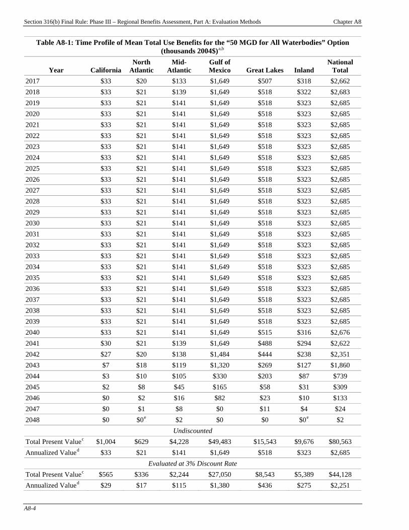
Section 316(b) Final Rule: Phase III – Regional Benefits Assessment, Part A: Evaluation Methods Chapter A8
A8-4
Table A8-1: Time Profile of Mean Total Use Benefits for the “50 MGD for All Waterbodies” Option (thousands 2004$)P
a,bP
Year California North
Atlantic Mid-
Atlantic Gulf of Mexico Great Lakes Inland
National Total
2017 $33 $20 $133 $1,649 $507 $318 $2,662 2018 $33 $21 $139 $1,649 $518 $322 $2,683 2019 $33 $21 $141 $1,649 $518 $323 $2,685 2020 $33 $21 $141 $1,649 $518 $323 $2,685 2021 $33 $21 $141 $1,649 $518 $323 $2,685 2022 $33 $21 $141 $1,649 $518 $323 $2,685 2023 $33 $21 $141 $1,649 $518 $323 $2,685 2024 $33 $21 $141 $1,649 $518 $323 $2,685 2025 $33 $21 $141 $1,649 $518 $323 $2,685 2026 $33 $21 $141 $1,649 $518 $323 $2,685 2027 $33 $21 $141 $1,649 $518 $323 $2,685 2028 $33 $21 $141 $1,649 $518 $323 $2,685 2029 $33 $21 $141 $1,649 $518 $323 $2,685 2030 $33 $21 $141 $1,649 $518 $323 $2,685 2031 $33 $21 $141 $1,649 $518 $323 $2,685 2032 $33 $21 $141 $1,649 $518 $323 $2,685 2033 $33 $21 $141 $1,649 $518 $323 $2,685 2034 $33 $21 $141 $1,649 $518 $323 $2,685 2035 $33 $21 $141 $1,649 $518 $323 $2,685 2036 $33 $21 $141 $1,649 $518 $323 $2,685 2037 $33 $21 $141 $1,649 $518 $323 $2,685 2038 $33 $21 $141 $1,649 $518 $323 $2,685 2039 $33 $21 $141 $1,649 $518 $323 $2,685 2040 $33 $21 $141 $1,649 $515 $316 $2,676 2041 $30 $21 $139 $1,649 $488 $294 $2,622 2042 $27 $20 $138 $1,484 $444 $238 $2,351 2043 $7 $18 $119 $1,320 $269 $127 $1,860 2044 $3 $10 $105 $330 $203 $87 $739 2045 $2 $8 $45 $165 $58 $31 $309 2046 $0 $2 $16 $82 $23 $10 $133 2047 $0 $1 $8 $0 $11 $4 $24 2048 $0 $0P
eP $2 $0 $0 $0P
eP $2
Undiscounted Total Present ValueP
cP $1,004 $629 $4,228 $49,483 $15,543 $9,676 $80,563
Annualized ValueP
dP $33 $21 $141 $1,649 $518 $323 $2,685
Evaluated at 3% Discount Rate Total Present ValueP
cP $565 $336 $2,244 $27,050 $8,543 $5,389 $44,128
Annualized ValueP
dP $29 $17 $115 $1,380 $436 $275 $2,251

Section 316(b) Final Rule: Phase III – Regional Benefits Assessment, Part A: Evaluation Methods Chapter A8
A8-5
Table A8-1: Time Profile of Mean Total Use Benefits for the “50 MGD for All Waterbodies” Option (thousands 2004$)P
a,bP
Year California North
Atlantic Mid-
Atlantic Gulf of Mexico Great Lakes Inland
National Total
Evaluated at 7% Discount Rate Total Present ValueP
cP $296 $165 $1,090 $13,631 $4,341 $2,786 $22,308
Annualized ValueP
dP $24 $13 $88 $1,098 $350 $224 $1,798
P
aP The estimate of the total use value of I&E reductions includes recreational and commercial fishing benefits. EPA
estimated non-use benefits qualitatively. P
bP Note that all monetary values in this table are expressed in thousands 2004$, since EPA did not adjust the values for
inflation. P
cP The total present value is equal to the sum of the values of the benefits realized in all years of the analysis,
discounted to 2007. P
dP The annualized value represents the total present value of the benefits of the regulation, distributed over a thirty year
period. P
eP Positive non-zero value less than $500.
Source: U.S. EPA analysis for this report.
Section 316(b) Final Rule: Phase III – Regional Benefits Assessment, Part A: Evaluation Methods Chapter A9
A9-1
Chapter A9: Threatened & Endangered Species Analysis Methods
Introduction Chapter Contents
A9-1 Listed Species Background .......................... A9-1 A9-1.1 Federally Listed Species
Definitions ...................................... A9-2 A9-1.2 Main Factors in Listing of Aquatic Species............................... A9-2 A9-1.3 “Incidental Take” Permits .............. A9-3 A9-2 Benefit Categories Applicable for Impacts on T&E Species...................................... .….A9-4 A9-3 Methods Available for Estimating the Economic Value Associated with I&E of T&E Species................................................. A9-5 A9-3.1 Estimating I&E Impacts on T&E Species ............................................ A9-5 A9-3.2 Economic Valuation Methods......... A9-5 A9-4 Issues in Estimating and Valuing Environmental Impacts from I&E on T&E Species............................................... A9-12 A9-4.1 Issues in Estimating the Size of the Population of Special Status Species .......................................... A9-12 A9-4.2 Issues Associated with Estimating I&E Contribution to the Cumulative Impact from All Stressors.................................. A9-12 A9-4.3 Issues Associated with Implementing an Economic Valuation Approach ...................... A9-12
Threatened and endangered (T&E) and other special status speciesPF
1FP can be adversely affected in several
ways by cooling water intake structures (CWIS). T&E species can suffer direct harm from impingement and entrainment (I&E), they can suffer indirect impacts if I&E at CWIS adversely affects another species upon which the T&E species relies (e.g., as a food source), or they can suffer impacts if the CWIS disrupts their critical habitat. The loss of individuals of listed species from CWIS is particularly important because, by definition, these species are already rare and at risk of irreversible decline because of other stressors. This chapter provides information relevant to an analysis of listed species in the context of the section 316(b) regulation; defines species considered as threatened, endangered, or of special concern; gives a brief overview of the potential for I&E-related adverse impacts on T&E species; and describes methods available for considering the economic value of such impacts. EPA was unable to evaluate the presence of T&E species near potentially regulated Phase III facilities because it was able to obtain only 20 Phase III studies. The lack of information on T&E species at Phase III facilities may be a function of this limited number of impingement and entrainment studies. However, a number of Phase II facilities have documented impingement and entrainment of T&E species. Chapters B-H provide information on the federally listed T&E species present in each region of EPA’s Phase III analysis. A9-1 Listed Species Background The federal government and individual states develop and maintain lists of species that are considered endangered, threatened, or of special concern. The federal and state lists are not identical: a state does not list a
P
1P To simplify the discussion, in this chapter EPA uses the terms “T&E species” and “special status species”
interchangeably to mean all species that are specifically listed as threatened or endangered, plus any other species that has been given a special status designation at the state or federal level.
Section 316(b) Final Rule: Phase III – Regional Benefits Assessment, Part A: Evaluation Methods Chapter A9
A9-2
species that is on the federal list if it is extirpated in the state. States may also list a species that is not on the federal list if the species is considered threatened or endangered at the state, but not federal, level. The federal trustees for T&E species are the Department of the Interior’s U.S. Fish and Wildlife Service (U.S. FWS) and National Oceanic and Atmospheric Administration (NOAA) Fisheries. Both departments are also referred to herein as the Services. The U.S. FWS is responsible for migratory birds and terrestrial and freshwater species (including plants), whereas NOAA Fisheries deals with marine species and anadromous fish (USFWS, 1996b). At the state level, the departments, agencies, or commissions with jurisdiction over T&E species include Fish and Game; Natural Resources; Fish and Wildlife Conservation; Fish, Wildlife and Parks; Game and Parks; Environmental Conservation; Conservation and Natural Resources; Parks and Wildlife; the states’ Natural Heritage Programs, and several others. In the remainder of this chapter, and in the regional sections of this document, EPA focuses on federally listed T&E species based on information in the U.S. FWS’ Threatened and Endangered Species System (TESS) database (USFWS, 2006a), available at HTUhttp://www.fws.gov/endangered/wildlife.htmlUTH. Information on both federal and state listed species is available online in the NatureServe database (NatureServe, 2006) at HTUhttp://www.natureserve.org/explorer/UTH. For additional information on state listed species, it is best to contact the T&E coordinator in the particular state of interest. A9-1.1 Federally Listed Species Definitions a. Threatened and endangered species A species is federally listed as “endangered” when it is likely to become extinct within the foreseeable future throughout all or part of its range if no immediate action is taken to protect it. A species is listed as “threatened” if it is likely to become endangered within the foreseeable future throughout all or most of its range if no action is taken to protect it. Species are selected for listing based on petitions, surveys by the Services or other agencies, and other substantiated reports or field studies. The 1973 Endangered Species Act (ESA) outlines detailed procedures used by the Services to list a species, including listing criteria, public comment periods, hearings, notifications, time limits for final action, and other related issues (USFWS, 1996b). A species is considered to be federally threatened or endangered if one or more of the following listing criteria apply (USFWS, 1996b):
< the species’ habitat or range is currently undergoing or is jeopardized by destruction, modification, or curtailment;
< the species is overused for commercial, recreational, scientific, or educational purposes; < the species’ existence is vulnerable because of predation or disease; < current regulatory mechanisms do not provide adequate protection; or < the continued existence of a species is affected by other natural or man-made factors.
b. Species of concern States and the federal government have also included species of “special concern” on their lists. These species have been selected because they are (1) rare or endemic, (2) in the process of being listed, (3) considered for listing in the future, (4) found in isolated and fragmented habitats, or (5) considered a unique or irreplaceable state resource. A9-1.2 Main Factors in Listing of Aquatic Species Numerous physical and biological stressors have resulted in the listing of aquatic species. The major factors include habitat destruction or modification, displacement of populations by exotic species, dam building and impoundments, increased siltation and turbidity in the water column, sedimentation, various point and non-point sources of pollution, poaching, and accidental catching. Some stresses, such as increased contaminant loads or
Section 316(b) Final Rule: Phase III – Regional Benefits Assessment, Part A: Evaluation Methods Chapter A9
A9-3
turbidity, can be alleviated by water quality programs such as the National Pollutant Discharge Elimination System (NPDES) or the current EPA efforts to develop Total Maximum Daily Loads (TMDLs). Other factors, such as dam building or habitat modifications for flood control purposes, are relatively permanent and therefore more difficult to mitigate. In addition to these major factors, negative effects of CWIS on some listed species have been documented. A9-1.3 “Incidental Take” Permits Congress amended the ESA in 1982 and established a legal mechanism authorizing the Services to issue permits to non-federal entities — including individuals, private businesses, corporations, local governments, state governments, and Tribal governments — who engage in the “incidental take” of federally-protected wildlife species (plants are not explicitly covered by this program). Incidental take is defined as take that is “incidental to, and not the purpose of, the carrying out of an otherwise lawful activity under local, State or Federal law.” Examples of lawful activities that may result in the incidental take of T&E species include developing private or state-owned land containing habitats used by federally-protected species, or the withdrawal of cooling water that may impinge or entrain federally-protected aquatic species present in surface waters. An integral part of the incidental take permit process is development of a Habitat Conservation Plan (HCP). An HCP provides a counterbalance to an incidental take by proposing measures to minimize or mitigate the impact and ensuring the long-term commitment of the non-federal entity to species conservation. HCPs often include conservation measures that benefit not only the target T&E species, but also proposed and candidate species, and other rare and sensitive species that are present within the plan area (USFWS and NMFS, 2000). The ESA stipulates the major points that must be addressed in an HCP, including the following (USFWS and NMFS, 2000):
< defining the potential impacts associated with the proposed taking of a federally-listed species; < describing the measures that the applicant will take to monitor, minimize, and mitigate these impacts,
including funding sourcesPF
2FP;
< analyzing alternative actions that could be taken by the applicant and reasons why those actions cannot be adopted; and
< describing additional measures that the Services may require as necessary or appropriate. HCP permits can be issued by the Services’ regional directors if:
< the taking will be incidental to an otherwise lawful activity; < any impacts will be minimized or fully mitigated; < the permittee provides adequate funding to fully implement the permit; < the incidental taking will not reduce the chances of survival or recovery of the T&E species; and < any other required measures are met.
The Services have published a detailed description of the incidental take permit process and the habitat conservation planning process (USFWS and NMFS, 2000). The federal incidental take permit program has only limited application within the context of the section 316(b) regulation because many T&E species (fish in particular) are listed mainly by states, not by the Services, and hence fall outside of the jurisdiction of this program.
P
2P Mitigation can include preserving critical habitats, restoring degraded former habitat, creating new habitats,
modifying land use practices to protect habitats, and establishing buffer areas around existing habitats.

Section 316(b) Final Rule: Phase III – Regional Benefits Assessment, Part A: Evaluation Methods Chapter A9
A9-4
A9-2 Benefit Categories Applicable for Impacts on T&E Species Estimating the economic benefits of helping to preserve T&E and other special status species, such as by reducing I&E impacts, is difficult due to a lack of knowledge of the ecological role of different T&E species and a relative paucity of economic studies focusing on the benefits of T&E preservation. Most of the wildlife economic literature focuses on recreational use benefits that may be irrelevant for valuation of T&E species because T&E species (e.g., the delta smelt in California) are not often targeted by recreational or commercial fishers. The numbers of special status species that are recreationally or commercially fished (e.g., shortnose sturgeon in the Delaware Estuary) have been so depleted that any use estimates associated with angling participation or landings data for recent years (or decades) would not be indicative of the species’ potential value for direct use if and when the population recovers. Nevertheless, there are some T&E species for which consumptive use-related benefits could be significant once the numbers of individuals are restored to levels that enable resumption of relevant uses. Based on their potential uses, T&E species can be divided into three broad categories:
< T&E species with high potential for consumptive uses. The components of total value of such species are likely to include consumptive, non-consumptive, and indirect use values, as well as existence and option values. Pacific salmon, a highly prized game species, is a good example of such species. In addition to having a high consumptive use value, this species is likely to have a high non-consumptive use value as well, because people who never go fishing may still watch salmon runs. The use value may actually dominate the total economic value of enhancing a T&E fish population for species like salmon. For example, Olsen et al. (1991) found that users contribute 65% to the total regional willingness-to-pay (WTP) value ($171 million in 1989$) for doubling the Columbia River salmon and steelhead runs. Non-users with zero probability of participation in the sport fishery contributed 25%. Non-users with some probability of future participation contributed the remaining 10%.
< T&E species that do not have consumptive uses, but are likely to have relatively large non-consumptive
and indirect use values. The total value of such species would include non-consumptive use and indirect values and existence values. Loggerhead sea turtles can represent such species. The non-consumptive use of loggerhead sea turtles may include photography or observation of nesting or swimming reptiles. For example, a study by Whitehead and Bloomquist (1992) reports that the average subjective probability that North Carolina residents will visit the North Carolina coast for non-consumptive use recreation is 0.498. Policies that protect loggerhead sea turtles may therefore enhance individual welfare for a large group of participants in turtle viewing and photography.
< T&E species whose total value is a pure non-use value. Some prominent T&E species with minimal or no
use values may have high non-use values. The bald eagle and the gray whale are examples of such species. Conversely, many T&E species with little or no use value are not well known or of significant public interest and therefore their non-use values may be challenging for individuals to report. Most obscure T&E species, which may have ecological, biological diversity, and other non-use values, are likely to fall into this category.
Non-use motives are often the principal source of benefits estimates for T&E species because many T&E species fall into the “obscure species” group. As described in greater detail in Chapter A3, motives often associated with non-use values held for T&E species include bequest (i.e., intergenerational equity) and existence (i.e., preservation and stewardship) values. These non-use values are not necessarily limited to T&E species, but I&E-related adverse impacts to these unique species would be locally or globally irreversible, leading to extinction being a relevant concern. Irreversible adverse impacts on unique resources are not a necessary condition for the presence of significant non-use values, but these attributes (e.g., uniqueness; irreversibility; and regional, national, or international significance) would generally be expected to generate relatively high non-use values (Harpman et al., 1993; Carson et al., 1999).
Section 316(b) Final Rule: Phase III – Regional Benefits Assessment, Part A: Evaluation Methods Chapter A9
A9-5
A9-3 Methods Available for Estimating the Economic Value Associated with I&E of T&E Species
Estimating the value of increased protection of T&E species from reducing I&E impacts requires the following steps:
< estimating I&E impacts on T&E species; and < attaching an economic value to changes in T&E status from reducing I&E impacts on species of concern
(e.g., increasing species population, preventing species extinction). A9-3.1 Estimating I&E Impacts on T&E Species Several cases of I&E of federally-protected species by CWIS are documented, including the delta smelt in the Sacramento-San Joaquin River Delta, sea turtles in the Delaware Estuary and elsewhere (NMFS, 2001b), shortnose sturgeon eggs and larvae in the Hudson River (NYSDEC, 2003), and pallid sturgeon eggs and larvae in the Great Rivers Basin (Dames & Moore, 1977). Mortality rates vary by species and life stage: it is estimated to range from 2 to 7% for impinged sea turtles (NMFS, 2001b), but mortality can be expected to be much higher for entrained eggs and larvae of the shortnose sturgeon and other special status fish species. The estimated yearly take of delta smelt by CWIS in the Sacramento-San Joaquin River Delta led to the development of a Habitat Conservation Plan as part of an incidental take permit application (Southern Energy Delta LLC, 2000). A9-3.2 Economic Valuation Methods Valuing impacts on special status species requires using nonmarket valuation methods to assign likely values to losses of these individuals. The fact that many of these species typically are not commercially or recreationally harvested (once they are listed) means no market value can be placed on their consumption. Benefits estimates are therefore often confined to non-use values for special status species. The total economic value of preserving species with potentially high use values (i.e., T&E salmon runs) should include both use and non-use values. Economic tools allowing estimates of both use and non-use values (e.g., stated preference methods) may be suitable for calculating the benefits of preserving T&E species. The relevant methods are briefly summarized below. It is necessary to note that the benefits of preserving T&E species estimated to date reflect a human-centered view; benefit cost analysis may need to be supplemented with other analyses when T&E species are involved because extinction is irreversible. a. Stated preference methods As described in Chapter A3, the only available way to directly estimate non-use values for special status species is through applying stated preference methods, such as the contingent valuation method (CVM). This method relies on statements of intended or hypothetical behavior elicited though surveys to value species. CVM has sometimes been criticized, especially in applications dating back a decade or more, because the analyst cannot verify whether the stated values are realistic and absent of various potential biases. CVM and other stated preference techniques (including conjoint analysis) have evolved and improved in recent years, however, and empirical evidence shows that the method can yield reliable (and perhaps even conservative) results where stated preference results are compared to those from revealed preference estimates (e.g., angling participation as observable behavior) (Carson et al., 1996). b. Benefit transfer approach Using a benefit transfer approach may be a viable option in some cases. By definition, benefit transfer involves extrapolating the benefits findings estimated from one analytic situation to another situation(s). The initial analytic situation is defined in terms of an environmental resource (e.g., T&E species), the policy variable(s) (e.g., changes in species status or population), and the benefiting populations being investigated. Only in ideal circumstances do the environmental resource and policy variables of the original study very closely match those
Section 316(b) Final Rule: Phase III – Regional Benefits Assessment, Part A: Evaluation Methods Chapter A9
A9-6
of the analytic situation to which a policy or regulatory analyst may wish to extrapolate study results. Despite discrepancies, this approach may provide useful insights into benefits to society from reducing stress on T&E species. The current approach to benefit transfers most often focuses on the meta-analysis of point estimates of the Hicksian or Marshalian surplus reported from original studies. If, for example, the number of candidate studies is small and the variation of characteristics among the studies is substantial, then meta-analysis is not feasible. This is likely to be the case when T&E species are involved, requiring a more careful consideration of analytic situations in the original and policy studies. If only one or a few studies are available, an analyst evaluates their transferability based on technical criteria developed by Desvousges et al. (1992). EPA illustrated the economic value to society of protecting T&E species by conducting a review of the contingent valuation (CV) literature that estimates WTP to protect those species. This review focused on those studies valuing those aquatic species that may be at risk of I&E by CWIS. EPA also identified studies that provide WTP estimates for fish-eating species, i.e., the bald eagle, peregrine falcon, and the whooping crane. These species may also be at risk because they rely to some degree on aquatic organisms as a food source. EPA used select studies identified in a meta-analysis that Loomis and White (1996) conducted as a literature base. Loomis and White included all rare or endangered species in their analysis, but EPA limited its own literature review to those studies that valued threatened or endangered aquatic species, or birds that consume aquatic species. Table A9-1 lists the 14 relevant CV studies that EPA identified and provides corresponding WTP estimates and selected study characteristics. WTP estimates represent either one-time payments, annual payments, or an annual payment in a 5-year program. The table indicates which of these payment types each WTP estimate represents, along with the corresponding value, inflated to 2004$. EPA also converted lump-sum payments and 5-year program annual payments into annualized values in order to aid in the comparison of values from all studies.TPF
3FPT
The identified valuation studies vary in terms of the species valued and the specific environmental change valued. Thirteen of these studies represent a total of 16 different species. In addition, one study (Walsh et al., 1985) estimates WTP for a group of 26 species. Most of these studies value prominent species well known by the public, such as salmon. The studies valued one of the following general types of environmental changes:
< avoidance of species loss/extinction; < species recovery/gain; < acceleration of the recovery process; < improvement of an area of a species’ habitat; and < increases in species population.
In order to compare consistent measures of WTP, EPA chose to use values that represent either annual or annualized WTP, which represent conservative estimates of consumer surplus. These measures are conservative because the value of preserving or improving populations of T&E species reported in T&E valuation studies has a wide range. Mean annual (or annualized) household WTP estimates of obscure aquatic species range from $7.89 (2004$) for the striped shiner (Boyle and Bishop, 1987) to $8.73 for the silvery minnow (Berrens et al., 1996). It is not likely that use values associated with these species are significant.
P
3P For each study that presents annual payments in a 5-year program, EPA calculated the present value of those
payments using a 3% discount rate, and annualized present day value over 25 years using the same discount factor. EPA considered lump-sum payments to represent present value, and thus merely annualized these payments using the same assumptions.
Section 316(b) Final Rule: Phase III – Regional Benefits Assessment, Part A: Evaluation Methods Chapter A9
A9-7
WTP for prominent fish species range from the relatively low estimate of $2.40 (2004$; Stevens et al., 1991), to $9.16 (Stevens et al., 1991); both values are mean non-user WTP for Atlantic salmon, and are annualized. Total user values are much higher for Atlantic salmon, as this species is commonly targeted by recreational anglers.TPF
4FPT
WTP estimates for fish-eating species (i.e., whooping crane, bald eagle, and peregrine falcon), which all have high non-use values (i.e., existence value), range from $4.60 (Carson et al., 1994) to $65.15 (Bowker and Stoll, 1988). It is important to note that the above WTP ranges are derived from studies that used various valuation scenarios and valued different types of environmental changes, and therefore should be viewed as approximate values as opposed to finite ranges. It may be possible to develop individual WTP ranges for a given species or species group based on the estimated changes in T&E status (e.g., species gain or recovery) from reducing I&E impacts and the applicable WTP values from existing studies. Once individual WTP for protecting T&E species or increasing their population is developed, the next step is to estimate total benefits from reducing I&E of the special status species. The analyst should apply the estimated WTP value to the relevant population groups to estimate the total value of improving protection of T&E species. The affected population may include both potential users and non-users, depending on species type. The relevant population may also include area residents, regional population, or, in exceptional cases (e.g., bald eagle), the U.S. population. The total value of improved protection of T&E species (e.g., preventing extinction or doubling the population size) should be then adjusted to reflect the percentage of cumulative environmental stress attributable to I&E. c. Cost of T&E species restoration Under specific circumstances it is possible to infer how much value society places on a program or activity by observing how much society is willing to forego (in out-of-pocket expenses and opportunity costs) to implement the program. For example, the costs borne by society to implement programs that preserve and restore special status species can, under select conditions, be interpreted as a measure of how much society values the outcomes it anticipates receiving. This approach is analogous to the broadly accepted revealed preference method of inferring values for private goods and services based on observed individual behavior. In the case of observed individual behavior, when a person willingly bears a cost (pays a price) to receive a good or service, then it is deduced that the person’s value for that acquired good or service must be at least as great as the price paid. That is, based on the presumption that individual behavior reflects the economic rationality of seeking to maximize utility (well-being), the person’s observed WTP must exceed the price paid, otherwise they would not have purchased that unit of the commodity. The approach described in this section uses the same premise, but applies it to societal choices rather than to a single individual’s choices. A critical issue with the approach is determining when it is likely that a specific public sector activity (or other form of collective action) does indeed reflect a “societal choice.” Not every policy enacted by a public sector entity can be interpreted as an indication of social choice. Hence, the costs imposed in such instances may not in any way reveal social values. For example, some regulatory actions may have monetized social costs that outweigh the monetized social benefits, but an action may be tougher because of legal requirements or other considerations. In such a case, asserting that the costs imposed reflect a lower bound estimate of the “value” of the action would not be accurate (the values may be less than the imposed costs). Alternatively, there are some regulatory programs for which the benefits greatly exceed costs, and in such instances using costs as a reflection of value would greatly understate social benefits.
TP
4PT See Chapter A5 of this report for details on recreational fishing values for Atlantic salmon.
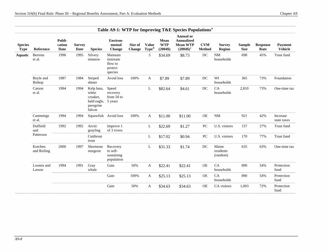
Section 316(b) Final Rule: Phase III – Regional Benefits Assessment, Part A: Evaluation Methods Chapter A9
A9-8
Table A9-1: WTP for Improving T&E Species PopulationsP
aP
Species Type Reference
Publi-cation Date
Survey Date Species
Environ-mental Change
Size of Change
Value TypeP
bP
Mean WTP
(2004$)
Annual or Annualized Mean WTP
(2004$)P
cP
CVM Method
Survey Region
Sample Size
Response Rate
Payment Vehicle
Berrens et al.
1996 1995 Silvery minnow
Maintain instream flow to protect species
5 $34.69 $8.73 DC NM households
698 45% Trust fund
Boyle and Bishop
1987 1984 Striped shiner
Avoid loss 100% A $7.89 $7.89 DC WI households
365 73% Foundation
Carson et al.
1994 1994 Kelp bass, white croaker, bald eagle, peregrine falcon
Speed recovery from 50 to 5 years
L $82.64 $4.61 DC CA households
2,810 73% One-time tax
Cummings et al.
1994 1994 Squawfish Avoid loss 100% A $11.00 $11.00 OE NM 921 42% Increase state taxes
1992 1992 Arctic grayling
Improve 1 of 3 rivers
L $22.69 $1.27 PC U.S. visitors 157 27% Trust fund Duffield and Patterson Cutthroat
trout L $17.02 $0.94 PC U.S. visitors 170 77% Trust fund
Kotchen and Reiling
2000 1997 Shortnose sturgeon
Recovery to self-sustaining population
L $31.33 $1.74 DC Maine residents (random)
635 63% One-time tax
1994 1991 Gray whale
Gain 50% A $22.41 $22.41 OE CA households
890 54% Protection fund
Gain 100% A $25.13 $25.13 OE CA households
890 54% Protection fund
Aquatic
Loomis and Larson
Gain 50% A $34.63 $34.63 OE CA visitors 1,003 72% Protection fund
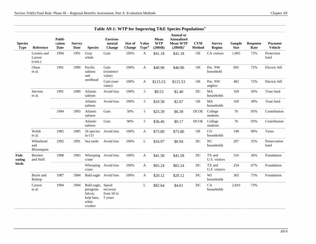
Section 316(b) Final Rule: Phase III – Regional Benefits Assessment, Part A: Evaluation Methods Chapter A9
A9-9
Table A9-1: WTP for Improving T&E Species PopulationsP
aP
Species Type Reference
Publi-cation Date
Survey Date Species
Environ-mental Change
Size of Change
Value TypeP
bP
Mean WTP
(2004$)
Annual or Annualized Mean WTP
(2004$)P
cP
CVM Method
Survey Region
Sample Size
Response Rate
Payment Vehicle
Loomis and Larson (cont.)
1994 1991 Gray whale
Gain 100% A $41.18 $41.18 OE CA visitors 1,003 72% Protection fund
Gain (existence value)
100% A $40.90 $40.90 OE Pac. NW household
695 72% Electric bill Olsen et al.
1991 1989 Pacific salmon and steelhead Gain (user
value) 100% A $115.53 $115.53 OE Pac. NW
anglers 482 72% Electric bill
1991 1989 Atlantic salmon
Avoid loss 100% 5 $9.53 $2.40 DC MA households
169 30% Trust fund
Atlantic salmon
Avoid loss 100% 5 $10.58 $2.67 OE MA households
169 30% Trust fund
1994 1993 Atlantic salmon
Gain 50% 5 $25.39 $6.39 DCOE College students
76 93% Contribution
Stevens et al.
Atlantic salmon
Gain 90% 5 $36.46 $9.17 DCOE College students
76 93% Contribution
Walsh et al.
1985 1985 26 species in CO
Avoid loss 100% A $75.80 $75.80 OE CO households
198 99% Taxes
Whitehead and Bloomquist
1992 1991 Sea turtle Avoid loss 100% L $16.97 $0.94 DC NC households
207 35% Preservation fund
1988 1983 Whooping crane
Avoid loss 100% A $41.58 $41.58 DC TX and U.S. visitors
316 36% Foundation Bowker and Stoll
Whooping crane
Avoid loss 100% A $65.24 $65.24 DC TX and U.S. visitors
254 67% Foundation
Boyle and Bishop
1987 1984 Bald eagle Avoid loss 100% A $20.12 $20.12 DC WI households
365 73% Foundation
Fish-eating birds
Carson et al.
1994 1994 Bald eagle, peregrine falcon, kelp bass, white croaker
Speed recovery from 50 to 5 years
L $82.64 $4.61 DC CA households
2,810 73%
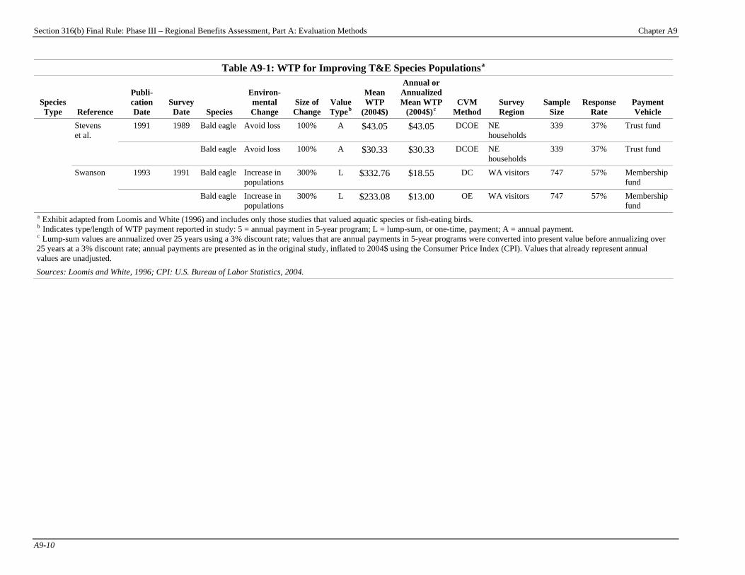
316(b) Final Rule: Phase III – Regional Benefits Assessment, Part A: Evaluation Methods Chapter A9
A9-10
1991 1989 Bald eagle Avoid loss 100% A $43.05 $43.05 DCOE NE households
339 37% Trust fund
Stevens et al.
Bald eagle Avoid loss 100% A $30.33 $30.33 DCOE NE households
339 37% Trust fund
1993 1991 Bald eagle Increase in populations
300% L $332.76 $18.55 DC WA visitors 747 57% Membership fund
Swanson
Bald eagle Increase in populations
300% L $233.08 $13.00 OE WA visitors 747 57% Membership fund
P
aP Exhibit adapted from Loomis and White (1996) and includes only those studies that valued aquatic species or fish-eating birds.
P
bP Indicates type/length of WTP payment reported in study: 5 = annual payment in 5-year program; L = lump-sum, or one-time, payment; A = annual payment.
P
cP Lump-sum values are annualized over 25 years using a 3% discount rate; values that are annual payments in 5-year programs were converted into present value before annualizing over
25 years at a 3% discount rate; annual payments are presented as in the original study, inflated to 2004$ using the Consumer Price Index (CPI). Values that already represent annual values are unadjusted. Sources: Loomis and White, 1996; CPI: U.S. Bureau of Labor Statistics, 2004.
Table A9-1: WTP for Improving T&E Species PopulationsP
aP
Species Type Reference
Publi-cation Date
Survey Date Species
Environ-mental Change
Size of Change
Value TypeP
bP
Mean WTP
(2004$)
Annual or Annualized Mean WTP
(2004$)P
cP
CVM Method
Survey Region
Sample Size
Response Rate
Payment Vehicle
Section
Section 316(b) Final Rule: Phase III – Regional Benefits Assessment, Part A: Evaluation Methods Chapter A9
A9-11
There are some public policy actions that can be suitably interpreted as expressions of societal preferences and values. In these instances, the incurred costs may be viewed as an indication of social values. The criteria to help identify when such situations arise include whether the actions taken are voluntary, or whether the actions reflect an open and broadly inclusive policy-making process that enables and encourages active participation by a broad spectrum of stakeholders. This is especially relevant where (1) plans and actions are developed in an inclusive, consensus-building manner; (2) implementation steps are pursued in an adaptive management framework that enables continuous feedback and refinement; or (3) the actions are ultimately supported by some positive indication of broad community support, such as voter approval of a referendum. In such instances, the policy choices made are the product of a broad-based, collective decision-making process, and such programs can be viewed as an expression of societal preferences. When programs or activities stem from such open collective processes, the actions (and costs incurred) may reflect the revealed preference of society. EPA’s method of valuing T&E species results in a three-step process. First, using the criteria above, EPA determines which action can be viewed as reflecting societal preferences. Next, estimates of costs incurred and anticipated from voluntary or other suitable collective actions taken to maintain and or increase the populations of T&E species (e.g., restoration of critical spawning or nursery habitat) are combined with estimates of the value of any foregone opportunities (i.e., opportunity costs, where direct costs are not involved) from additional actions required to achieve the T&E population objectives (e.g., maintaining instream flows for a species instead of providing water for agricultural diversions). This resulting total social cost provides a cumulative estimate of society’s valuation of the preservation and enhancement of the T&E species affected by the actions. Categories of actions that would be addressed in this step could include private and public expenditures on habitat restoration/population enhancement programs, funds that have been allocated for such actions through legislative appropriations or public referenda (even if not yet expended), or resources allocated through a formal project evaluation and selection process designed to allocate limited resources such as those used by numerous state and federal resource management agencies. Third, the numbers of the T&E organisms that are expected to benefit from the identified actions, as measured by the increased production or avoided losses of individuals, are estimated to place the valuation estimates in context. If dollar per organism results are required for a valuation analysis, as is the case in this analysis, the estimates from the second step can be divided by the increased production (avoided loss) estimate from the third step to provide such results. The economic foundations for using this approach to value T&E species are established through the widespread recognition and acceptance of revealed preference data as a source of nonmarket information that is acceptable for the valuation of resources. As discussed above, in EPA’s approach, valuation estimates rely on the costs of actions or the value of foregone opportunities that are voluntarily undertaken or that have been approved through extensive public input and review (and developed in a consensus-oriented approach). With these sources of data, the method avoids the well-established problems associated with using “costs” as a measure of “value” — a problem that can arise when the cost is realized involuntarily (e.g., avoided cost-based measures of value). Specifically, because of the available evidence of the public’s acceptance and willingness to incur the opportunity costs associated with the actions that are selected for evaluation, the fundamental criteria for defining the value of any resource are satisfied. One issue that arises with the use of the method is that it is not clear that the resulting values can be distinctly categorized as direct use or non-use values because the underlying actions benefiting the T&E species could reflect an expressed mix of non-use values (e.g., preservation and existence) and discounted future use values (i.e., the actions are seen as an “investment” that could return the species to levels at which direct use would be permitted). It is believed that results could provide an approximation of the total use value for the T&E species in question.
Section 316(b) Final Rule: Phase III – Regional Benefits Assessment, Part A: Evaluation Methods Chapter A9
A9-12
A9-4 Issues in Estimating and Valuing Environmental Impacts from I&E on T&E Species
Several technical and conceptual issues are associated with valuing I&E impacts on T&E species:
< issues associated with estimating the size of a species’ population; < issues associated with estimating the contribution of I&E to the cumulative impacts of all stressors; and < issues associated with implementing an economic valuation approach.
A9-4.1 Issues in Estimating the Size of the Population of Special Status Species Difficulties in estimating the number of individuals or size of the population of special status fish present in a given location are often very difficult for numerous reasons, including the following:
< the act of monitoring a T&E species is problematic in and of itself because, by definition, the species is rare, and monitoring can result in some harm to the species. Researchers and federal agencies can therefore be reluctant to undertake such monitoring;
< monitoring programs typically focus only on harvested species and so do not provide any information with regard to non-harvested T&E species that are subject to I&E; and
< the number of individuals of a T&E species may be so low that they rarely or never show up in monitoring programs.
Deriving population estimates from existing monitoring programs often means extrapolating monitoring sample catches to the population as a whole. The variance in estimates is likely to be very high because of several assumptions that must be met when extrapolating monitoring sample catches to population estimates in order to create an accurate estimate:
< species are completely recruited and vulnerable to the gear (i.e., are large enough to be retained by the mesh and do not preferentially occupy habitats not sampled) or selectivity of the gear by size is known;
< sampling fixed locations for species approximates random sampling; < species are uniformly distributed through the water column; < volume filtered by sampling trawls can be accurately estimated; and < volumes of water can be estimated for each embayment in the habitat range for the species.
A9-4.2 Issues Associated with Estimating I&E Contribution to the Cumulative Impact from All Stressors There are also issues associated with estimating the relative contribution of I&E to the total impact of all stressors on T&E species:
< Because, as outlined above, the size of populations of T&E species is hard to measure even if I&E data are available from facilities with cooling water intake structures, it may be difficult to determine how much of an impact I&E has on population levels. For very rare species, even relatively low levels of I&E may be important.
< There are often a number of stressors that harm or limit populations of special status fish. Even if significant numbers of fish are lost to I&E, other factors may still have a greater role in determining populations levels. For example, if lack of spawning areas is limiting population growth of a species, then reducing I&E of that species may not increase the population.
A9-4.3 Issues Associated with Implementing an Economic Valuation Approach a. Issues associated with benefit transfer approach The following issues may arise when using a benefit transfer approach:

Section 316(b) Final Rule: Phase III – Regional Benefits Assessment, Part A: Evaluation Methods Chapter A9
A9-13
< Some studies estimated WTP for multiple species. Values established by Walsh et al. (1985), Olsen et al. (1991), and Carson et al. (1994) are for groups of T&E species, and therefore transferring values from these studies to particular species may not be feasible.
< The type of environmental change valued in the study may not match the environmental changes resulting
from reducing I&E impacts. As noted above, previous T&E valuation studies addressed one of the following qualitative changes in T&E status: • avoidance of species loss/extinction; • species recovery/gain; • acceleration of the recovery process; • improvement of an area of a species’ habitat; and • increases in species population.
< The size of the environmental change that the hypothetical scenario defines is also vital for developing WTP estimates. Several studies describe programs that avoid the loss of a species. This outcome may be considered a 100% improvement with respect to the alternative, extinction, but the restoration of a species or the increase in population may be specified at any level (e.g., 50%, 300%). Swanson (1993) estimated a 300% increase in bald eagle populations and Boyle and Bishop (1987) estimated WTP to avoid the possibility of bald eagle extinction in Wisconsin (cited in Loomis and White, 1996). Although avoiding extinction may be considered a 100% improvement, this environmental change is not comparable to the 300% increase in existing populations. Preventing regional extinction is quite different than realizing a nominal increase in species population (in which the alternative is not necessarily species loss). Since different studies measure different types of improvements, creating a common metric with which to transfer values can be difficult.
< Although a considerable amount of CV literature has valued T&E species, such research is largely limited
to species with high consumptive use or non-use values. They either have high recreational or commercial value, or are popularly valued as significant species for various reasons (e.g., national symbol, aesthetics). Transferring these values to other species may not be appropriate. Many T&E species that are likely to be affected by I&E (either federal or state-listed) are obscure, and WTP for their preservation has not been estimated.
b. Issues associated with cost of restoration approach The following issues may arise when using a cost of restoration approach:
< “Restoration” programs need not be relied on exclusively to infer societal WTP to preserve special status species. In many instances, other programs or restrictions are used in lieu of (or in conjunction with) restoration programs. In these cases, the costs associated with the restoration components also reveal a WTP. Collecting all of these components may be challenging.
< Costs directed at a special status species must be isolated from program elements intended to address
other species or problems. In a multifaceted restoration or use restriction program, the percentage of costs used mainly to target restoration of special status species as opposed to other ecosystem benefits needs to be estimated. Separating these components out for an accurate valuation can be challenging.
< Estimates of the change in species abundance associated with the program must be developed, since the
size of the change in species abundance is necessary to determine societal WTP per individual. Often targets are set to abundance levels that existed before a significant decline in populations. However, a habitat restoration program may target restoration of special status species, but might not target a specific population size making calculation of societal WTP per individual difficult.

Section 316(b) Final Rule: Phase III – Regional Benefits Assessment
Part B: California
Section 316(b) Final Rule: Phase III – Regional Benefits Assessment, Part B: California Chapter B1
B1-1
Chapter B1: Background Introduction This chapter presents an overview of the potential Phase III existing facilities in the California study region and summarizes their key cooling water and compliance characteristics. For further discussion of the technical and compliance characteristics of potential Phase III existing facilities, refer to the Economic Analysis for the Final Section 316(b) Rule for Phase III Facilities and the Technical Development Document for the Final Section 316(b) Rule for Phase III Facilities (U.S. EPA, 2006a,c).
Chapter Contents B1-1 Facility Characteristics..................................B1-1
B1-1 Facility Characteristics The California Regional Study includes four sample facilities that are potentially subject to the national standards for Phase III existing facilities. Figure B1-1 presents a map of these facilities. All four facilities are manufacturing facilities. Industry-wide, these four sample facilities represent nine manufacturing facilities.PF
1FP
P
1P EPA applied sample weights to the survey respondents to account for non-sampled facilities and facilities that did
not respond to the survey. For more information on EPA’s 2000 Section 316(b) Industry Survey, please refer to the Information Collection Request (U.S. EPA, 2000b).
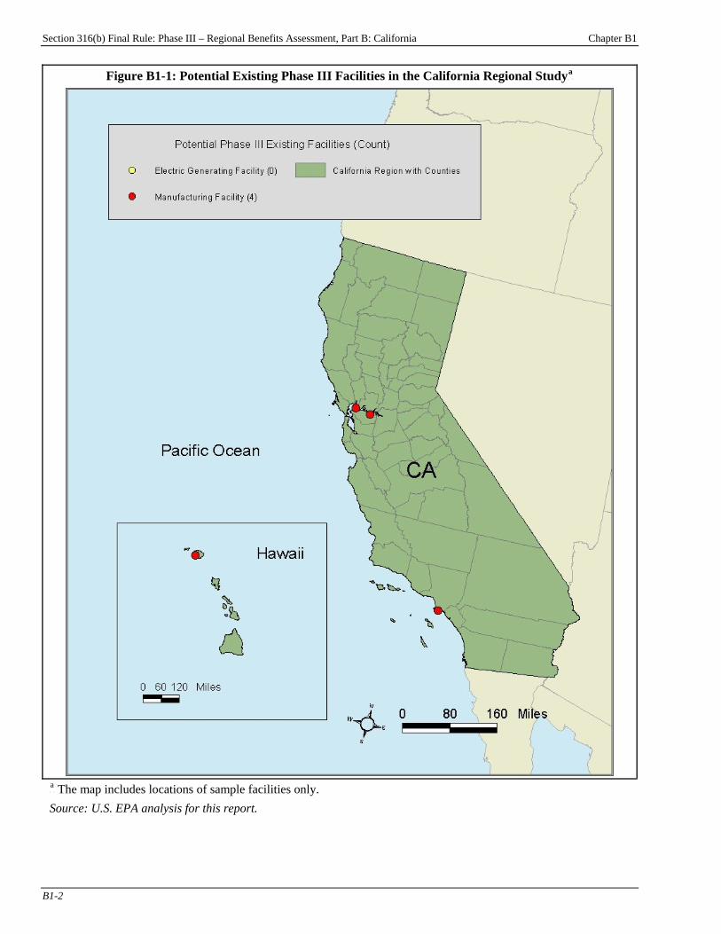
Section 316(b) Final Rule: Phase III – Regional Benefits Assessment, Part B: California Chapter B1
B1-2
Figure B1-1: Potential Existing Phase III Facilities in the California Regional StudyP
aP
P
aP The map includes locations of sample facilities only.
Source: U.S. EPA analysis for this report.

Section 316(b) Final Rule: Phase III – Regional Benefits Assessment, Part B: California Chapter B1
B1-3
Table B1-1 summarizes key technical and compliance characteristics for all potentially regulated Phase III existing facilities in the California study region for the regulatory analysis options considered by EPA for this rule (the “50 MGD for All Waterbodies” option, the “200 MGD for All Waterbodies” option, and the “100 MGD for Certain Waterbodies” option). Facilities with a design intake flow below the three applicability thresholds would be subject to permitting based on best professional judgment and are excluded from EPA’s analyses.PF
2FP Therefore,
a different number of facilities is affected under each option. Table B1-1 shows that nine Phase III existing facilities in the California study region would potentially be subject to the national requirements. Under the “50 MGD for All Waterbodies” option, the most inclusive of the regulatory analysis options, only one facility would be subject to the national requirements for Phase III existing facilities. Under the less inclusive “200 MGD for All Waterbodies” option and the “100 MGD for Certain Waterbodies” option (which includes all facilities in the California study region), no facilities would be subject to the national requirements. One facility in the California study region has a recirculating system in the baseline. Data on design intake flow for the California study facilities have been withheld due to data confidentiality reasons.
Table B1-1: Technical and Compliance Characteristics of Phase III Existing Facilities (sample-weighted) Regulatory Analysis Options All Potentially
Regulated Facilities
50 MGD All
200 MGD All
100 MGD CWB
Total Number of Facilities (sample-weighted) 9 1 - - Number of Facilities with Recirculating System in Baseline 1 - - - Design Intake Flow (MGD) wP
aP wP
aP - -
Number of Facilities by Compliance Response New larger intake structure with fine mesh and fish H&R 1 1 - - Passive fine mesh screens - - - - None 8 - - -
Compliance Cost, Discounted at 3%P
bP
$1.79 $0.40 $0.00 $0.00
Compliance Cost, Discounted at 7%P
bP
$1.69 $0.42 $0.00 $0.00 P
aP Data withheld because of confidentiality reasons.
P
bP Annualized pre-tax compliance cost (2004$, millions).
Sources: U.S. EPA, 2000b; U.S. EPA analysis for this report.
P
2P Also excluded are facilities that are estimated to be baseline closures. For additional information on EPA’s
baseline closure analyses, please refer to the Economic Analysis for the Final Section 316(b) Rule for Phase III Facilities (U.S. EPA, 2006a).
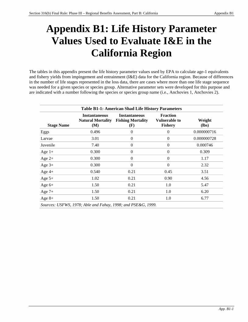
Section 316(b) Final Rule: Phase III – Regional Benefits Assessment, Part B: California Appendix B1
App. B1-1
Appendix B1: Life History Parameter Values Used to Evaluate I&E in the
California Region The tables in this appendix present the life history parameter values used by EPA to calculate age-1 equivalents and fishery yields from impingement and entrainment (I&E) data for the California region. Because of differences in the number of life stages represented in the loss data, there are cases where more than one life stage sequence was needed for a given species or species group. Alternative parameter sets were developed for this purpose and are indicated with a number following the species or species group name (i.e., Anchovies 1, Anchovies 2).
Table B1-1: American Shad Life History Parameters
Stage Name
Instantaneous Natural Mortality
(M)
Instantaneous Fishing Mortality
(F)
Fraction Vulnerable to
Fishery Weight
(lbs) Eggs 0.496 0 0 0.000000716 Larvae 3.01 0 0 0.000000728 Juvenile 7.40 0 0 0.000746 Age 1+ 0.300 0 0 0.309 Age 2+ 0.300 0 0 1.17 Age 3+ 0.300 0 0 2.32 Age 4+ 0.540 0.21 0.45 3.51 Age 5+ 1.02 0.21 0.90 4.56 Age 6+ 1.50 0.21 1.0 5.47 Age 7+ 1.50 0.21 1.0 6.20 Age 8+ 1.50 0.21 1.0 6.77 Sources: USFWS, 1978; Able and Fahay, 1998; and PSE&G, 1999.
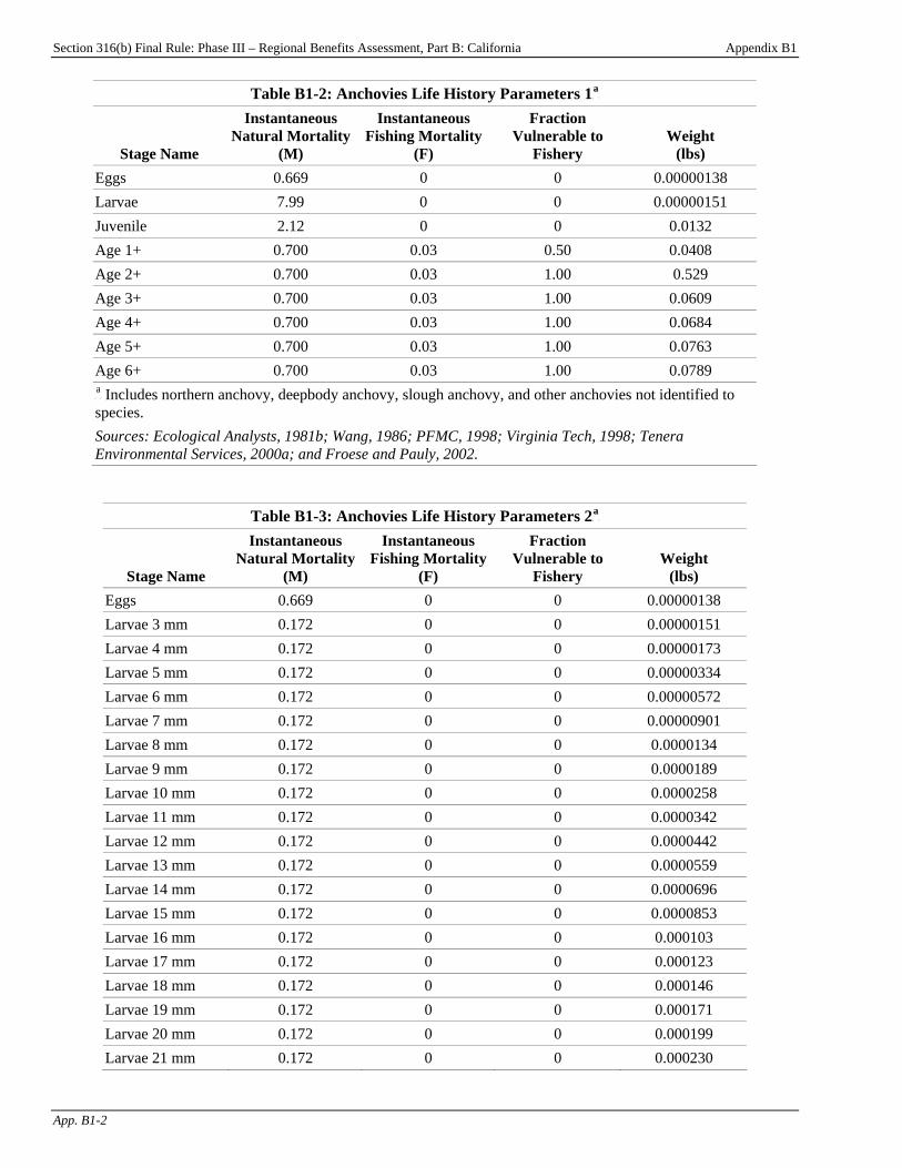
Section 316(b) Final Rule: Phase III – Regional Benefits Assessment, Part B: California Appendix B1
App. B1-2
Table B1-2: Anchovies Life History Parameters 1P
aP
Stage Name
Instantaneous Natural Mortality
(M)
Instantaneous Fishing Mortality
(F)
Fraction Vulnerable to
Fishery Weight
(lbs) Eggs 0.669 0 0 0.00000138 Larvae 7.99 0 0 0.00000151 Juvenile 2.12 0 0 0.0132 Age 1+ 0.700 0.03 0.50 0.0408 Age 2+ 0.700 0.03 1.00 0.529 Age 3+ 0.700 0.03 1.00 0.0609 Age 4+ 0.700 0.03 1.00 0.0684 Age 5+ 0.700 0.03 1.00 0.0763 Age 6+ 0.700 0.03 1.00 0.0789 P
aP Includes northern anchovy, deepbody anchovy, slough anchovy, and other anchovies not identified to
species. Sources: Ecological Analysts, 1981b; Wang, 1986; PFMC, 1998; Virginia Tech, 1998; Tenera Environmental Services, 2000a; and Froese and Pauly, 2002.
Table B1-3: Anchovies Life History Parameters 2P
aP
Stage Name
Instantaneous Natural Mortality
(M)
Instantaneous Fishing Mortality
(F)
Fraction Vulnerable to
Fishery Weight
(lbs) Eggs 0.669 0 0 0.00000138 Larvae 3 mm 0.172 0 0 0.00000151 Larvae 4 mm 0.172 0 0 0.00000173 Larvae 5 mm 0.172 0 0 0.00000334 Larvae 6 mm 0.172 0 0 0.00000572 Larvae 7 mm 0.172 0 0 0.00000901 Larvae 8 mm 0.172 0 0 0.0000134 Larvae 9 mm 0.172 0 0 0.0000189 Larvae 10 mm 0.172 0 0 0.0000258 Larvae 11 mm 0.172 0 0 0.0000342 Larvae 12 mm 0.172 0 0 0.0000442 Larvae 13 mm 0.172 0 0 0.0000559 Larvae 14 mm 0.172 0 0 0.0000696 Larvae 15 mm 0.172 0 0 0.0000853 Larvae 16 mm 0.172 0 0 0.000103 Larvae 17 mm 0.172 0 0 0.000123 Larvae 18 mm 0.172 0 0 0.000146 Larvae 19 mm 0.172 0 0 0.000171 Larvae 20 mm 0.172 0 0 0.000199 Larvae 21 mm 0.172 0 0 0.000230

Section 316(b) Final Rule: Phase III – Regional Benefits Assessment, Part B: California Appendix B1
App. B1-3
Table B1-3: Anchovies Life History Parameters 2P
aP
Stage Name
Instantaneous Natural Mortality
(M)
Instantaneous Fishing Mortality
(F)
Fraction Vulnerable to
Fishery Weight
(lbs) Larvae 22 mm 0.172 0 0 0.000264 Larvae 23 mm 0.172 0 0 0.000301 Larvae 24 mm 0.172 0 0 0.000341 Larvae 25 mm 0.172 0 0 0.000385 Larvae 26 mm 0.172 0 0 0.000432 Larvae 27 mm 0.172 0 0 0.000483 Larvae 28 mm 0.172 0 0 0.000538 Larvae 29 mm 0.172 0 0 0.000597 Larvae 30 mm 0.172 0 0 0.000659 Larvae 31 mm 0.172 0 0 0.000726 Larvae 32 mm 0.172 0 0 0.000798 Larvae 33 mm 0.172 0 0 0.000873 Larvae 34 mm 0.172 0 0 0.000954 Larvae 35 mm 0.172 0 0 0.00104 Larvae 36 mm 0.172 0 0 0.00113 Larvae 37 mm 0.172 0 0 0.00122 Larvae 38 mm 0.172 0 0 0.00132 Larvae 39 mm 0.172 0 0 0.00143 Larvae 40 mm 0.172 0 0 0.00154 Larvae 41 mm 1.249 0 0 0.00166 Larvae 59 mm 0.208 0 0 0.00485 Juvenile 2.12 0 0 0.0132 Age 1+ 0.700 0.03 0.50 0.0408 Age 2+ 0.700 0.03 1.0 0.0529 Age 3+ 0.700 0.03 1.0 0.0609 Age 4+ 0.700 0.03 1.0 0.0684 Age 5+ 0.700 0.03 1.0 0.0763 Age 6+ 0.700 0.03 1.0 0.0789 P
aP Includes northern anchovy.
Sources: Ecological Analysts, 1980b, 1981b; Wang, 1986; PFMC, 1998; Tenera Environmental Services, 2000a; and Froese and Pauly, 2002.
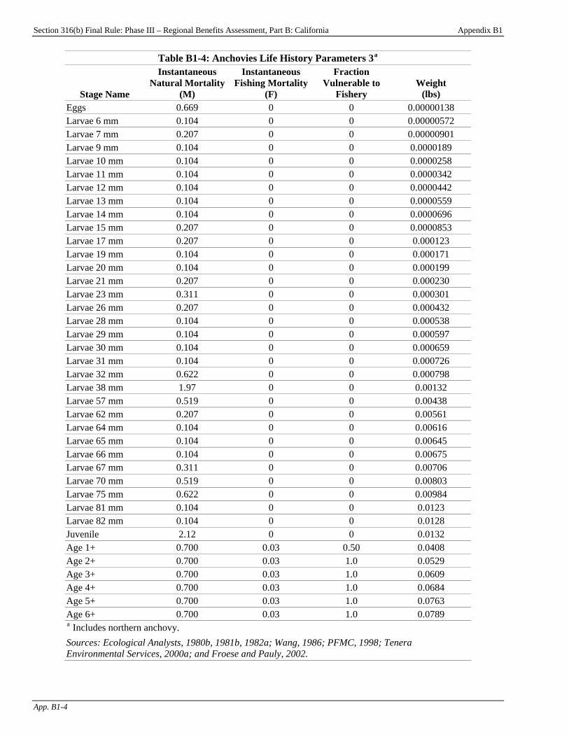
Section 316(b) Final Rule: Phase III – Regional Benefits Assessment, Part B: California Appendix B1
App. B1-4
Table B1-4: Anchovies Life History Parameters 3P
aP
Stage Name
Instantaneous Natural Mortality
(M)
Instantaneous Fishing Mortality
(F)
Fraction Vulnerable to
Fishery Weight
(lbs) Eggs 0.669 0 0 0.00000138 Larvae 6 mm 0.104 0 0 0.00000572 Larvae 7 mm 0.207 0 0 0.00000901 Larvae 9 mm 0.104 0 0 0.0000189 Larvae 10 mm 0.104 0 0 0.0000258 Larvae 11 mm 0.104 0 0 0.0000342 Larvae 12 mm 0.104 0 0 0.0000442 Larvae 13 mm 0.104 0 0 0.0000559 Larvae 14 mm 0.104 0 0 0.0000696 Larvae 15 mm 0.207 0 0 0.0000853 Larvae 17 mm 0.207 0 0 0.000123 Larvae 19 mm 0.104 0 0 0.000171 Larvae 20 mm 0.104 0 0 0.000199 Larvae 21 mm 0.207 0 0 0.000230 Larvae 23 mm 0.311 0 0 0.000301 Larvae 26 mm 0.207 0 0 0.000432 Larvae 28 mm 0.104 0 0 0.000538 Larvae 29 mm 0.104 0 0 0.000597 Larvae 30 mm 0.104 0 0 0.000659 Larvae 31 mm 0.104 0 0 0.000726 Larvae 32 mm 0.622 0 0 0.000798 Larvae 38 mm 1.97 0 0 0.00132 Larvae 57 mm 0.519 0 0 0.00438 Larvae 62 mm 0.207 0 0 0.00561 Larvae 64 mm 0.104 0 0 0.00616 Larvae 65 mm 0.104 0 0 0.00645 Larvae 66 mm 0.104 0 0 0.00675 Larvae 67 mm 0.311 0 0 0.00706 Larvae 70 mm 0.519 0 0 0.00803 Larvae 75 mm 0.622 0 0 0.00984 Larvae 81 mm 0.104 0 0 0.0123 Larvae 82 mm 0.104 0 0 0.0128 Juvenile 2.12 0 0 0.0132 Age 1+ 0.700 0.03 0.50 0.0408 Age 2+ 0.700 0.03 1.0 0.0529 Age 3+ 0.700 0.03 1.0 0.0609 Age 4+ 0.700 0.03 1.0 0.0684 Age 5+ 0.700 0.03 1.0 0.0763 Age 6+ 0.700 0.03 1.0 0.0789 P
aP Includes northern anchovy.
Sources: Ecological Analysts, 1980b, 1981b, 1982a; Wang, 1986; PFMC, 1998; Tenera Environmental Services, 2000a; and Froese and Pauly, 2002.
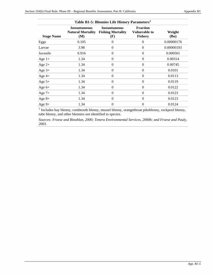
Section 316(b) Final Rule: Phase III – Regional Benefits Assessment, Part B: California Appendix B1
App. B1-5
Table B1-5: Blennies Life History ParametersP
aP
Stage Name
Instantaneous Natural Mortality
(M)
Instantaneous Fishing Mortality
(F)
Fraction Vulnerable to
Fishery Weight
(lbs) Eggs 0.105 0 0 0.00000176 Larvae 3.98 0 0 0.00000193 Juvenile 0.916 0 0 0.000501 Age 1+ 1.34 0 0 0.00314 Age 2+ 1.34 0 0 0.00745 Age 3+ 1.34 0 0 0.0101 Age 4+ 1.34 0 0 0.0113 Age 5+ 1.34 0 0 0.0119 Age 6+ 1.34 0 0 0.0122 Age 7+ 1.34 0 0 0.0123 Age 8+ 1.34 0 0 0.0123 Age 9+ 1.34 0 0 0.0124 P
aP Includes bay blenny, combtooth blenny, mussel blenny, orangethroat pikeblenny, rockpool blenny,
tube blenny, and other blennies not identified to species. Sources: Froese and Binohlan, 2000; Tenera Environmental Services, 2000b; and Froese and Pauly, 2003.
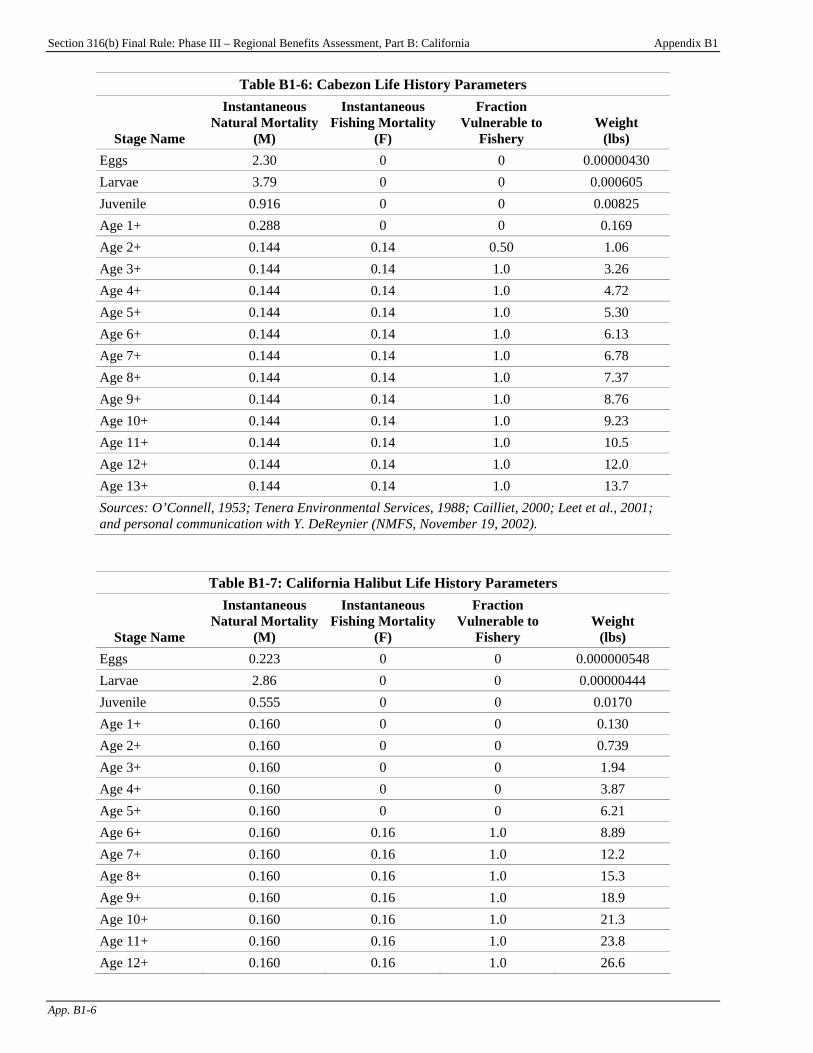
Section 316(b) Final Rule: Phase III – Regional Benefits Assessment, Part B: California Appendix B1
App. B1-6
Table B1-6: Cabezon Life History Parameters
Stage Name
Instantaneous Natural Mortality
(M)
Instantaneous Fishing Mortality
(F)
Fraction Vulnerable to
Fishery Weight
(lbs) Eggs 2.30 0 0 0.00000430 Larvae 3.79 0 0 0.000605 Juvenile 0.916 0 0 0.00825 Age 1+ 0.288 0 0 0.169 Age 2+ 0.144 0.14 0.50 1.06 Age 3+ 0.144 0.14 1.0 3.26 Age 4+ 0.144 0.14 1.0 4.72 Age 5+ 0.144 0.14 1.0 5.30 Age 6+ 0.144 0.14 1.0 6.13 Age 7+ 0.144 0.14 1.0 6.78 Age 8+ 0.144 0.14 1.0 7.37 Age 9+ 0.144 0.14 1.0 8.76 Age 10+ 0.144 0.14 1.0 9.23 Age 11+ 0.144 0.14 1.0 10.5 Age 12+ 0.144 0.14 1.0 12.0 Age 13+ 0.144 0.14 1.0 13.7 Sources: O’Connell, 1953; Tenera Environmental Services, 1988; Cailliet, 2000; Leet et al., 2001; and personal communication with Y. DeReynier (NMFS, November 19, 2002).
Table B1-7: California Halibut Life History Parameters
Stage Name
Instantaneous Natural Mortality
(M)
Instantaneous Fishing Mortality
(F)
Fraction Vulnerable to
Fishery Weight
(lbs) Eggs 0.223 0 0 0.000000548 Larvae 2.86 0 0 0.00000444 Juvenile 0.555 0 0 0.0170 Age 1+ 0.160 0 0 0.130 Age 2+ 0.160 0 0 0.739 Age 3+ 0.160 0 0 1.94 Age 4+ 0.160 0 0 3.87 Age 5+ 0.160 0 0 6.21 Age 6+ 0.160 0.16 1.0 8.89 Age 7+ 0.160 0.16 1.0 12.2 Age 8+ 0.160 0.16 1.0 15.3 Age 9+ 0.160 0.16 1.0 18.9 Age 10+ 0.160 0.16 1.0 21.3 Age 11+ 0.160 0.16 1.0 23.8 Age 12+ 0.160 0.16 1.0 26.6
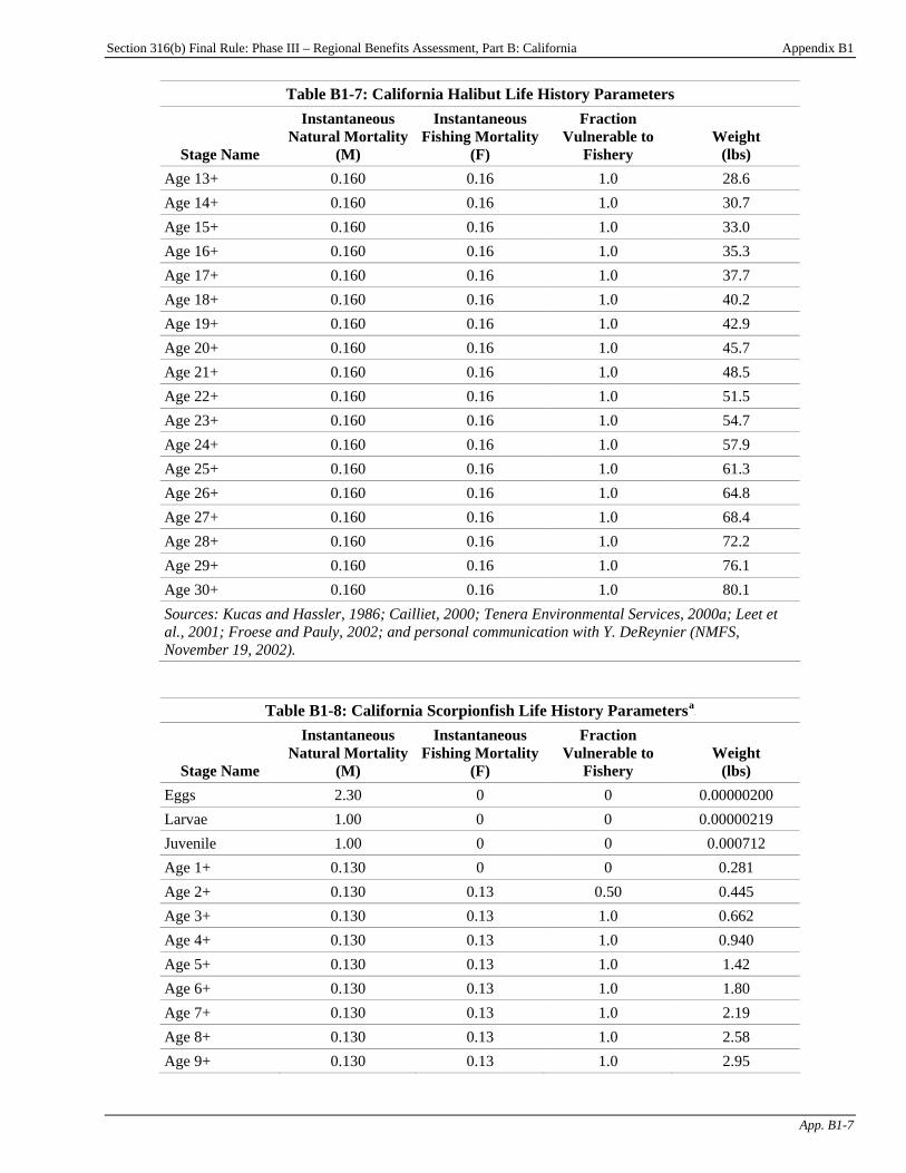
Section 316(b) Final Rule: Phase III – Regional Benefits Assessment, Part B: California Appendix B1
App. B1-7
Table B1-7: California Halibut Life History Parameters
Stage Name
Instantaneous Natural Mortality
(M)
Instantaneous Fishing Mortality
(F)
Fraction Vulnerable to
Fishery Weight
(lbs) Age 13+ 0.160 0.16 1.0 28.6 Age 14+ 0.160 0.16 1.0 30.7 Age 15+ 0.160 0.16 1.0 33.0 Age 16+ 0.160 0.16 1.0 35.3 Age 17+ 0.160 0.16 1.0 37.7 Age 18+ 0.160 0.16 1.0 40.2 Age 19+ 0.160 0.16 1.0 42.9 Age 20+ 0.160 0.16 1.0 45.7 Age 21+ 0.160 0.16 1.0 48.5 Age 22+ 0.160 0.16 1.0 51.5 Age 23+ 0.160 0.16 1.0 54.7 Age 24+ 0.160 0.16 1.0 57.9 Age 25+ 0.160 0.16 1.0 61.3 Age 26+ 0.160 0.16 1.0 64.8 Age 27+ 0.160 0.16 1.0 68.4 Age 28+ 0.160 0.16 1.0 72.2 Age 29+ 0.160 0.16 1.0 76.1 Age 30+ 0.160 0.16 1.0 80.1 Sources: Kucas and Hassler, 1986; Cailliet, 2000; Tenera Environmental Services, 2000a; Leet et al., 2001; Froese and Pauly, 2002; and personal communication with Y. DeReynier (NMFS, November 19, 2002).
Table B1-8: California Scorpionfish Life History ParametersP
aP
Stage Name
Instantaneous Natural Mortality
(M)
Instantaneous Fishing Mortality
(F)
Fraction Vulnerable to
Fishery Weight
(lbs) Eggs 2.30 0 0 0.00000200 Larvae 1.00 0 0 0.00000219 Juvenile 1.00 0 0 0.000712 Age 1+ 0.130 0 0 0.281 Age 2+ 0.130 0.13 0.50 0.445 Age 3+ 0.130 0.13 1.0 0.662 Age 4+ 0.130 0.13 1.0 0.940 Age 5+ 0.130 0.13 1.0 1.42 Age 6+ 0.130 0.13 1.0 1.80 Age 7+ 0.130 0.13 1.0 2.19 Age 8+ 0.130 0.13 1.0 2.58 Age 9+ 0.130 0.13 1.0 2.95
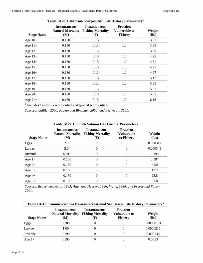
Section 316(b) Final Rule: Phase III – Regional Benefits Assessment, Part B: California Appendix B1
App. B1-8
Table B1-8: California Scorpionfish Life History ParametersP
aP
Stage Name
Instantaneous Natural Mortality
(M)
Instantaneous Fishing Mortality
(F)
Fraction Vulnerable to
Fishery Weight
(lbs) Age 10+ 0.130 0.13 1.0 3.31 Age 11+ 0.130 0.13 1.0 3.65 Age 12+ 0.130 0.13 1.0 3.96 Age 13+ 0.130 0.13 1.0 4.25 Age 14+ 0.130 0.13 1.0 4.51 Age 15+ 0.130 0.13 1.0 4.75 Age 16+ 0.130 0.13 1.0 4.97 Age 17+ 0.130 0.13 1.0 5.17 Age 18+ 0.130 0.13 1.0 5.35 Age 19+ 0.130 0.13 1.0 5.51 Age 20+ 0.130 0.13 1.0 5.65 Age 21+ 0.130 0.13 1.0 6.18 P
aP Includes California scorpionfish and spotted scorpionfish.
Sources: Cailliet, 2000; Froese and Binohlan, 2000; and Leet et al., 2001.
Table B1-9: Chinook Salmon Life History Parameters
Stage Name
Instantaneous Natural Mortality
(M)
Instantaneous Fishing Mortality
(F)
Fraction Vulnerable to Fishery
Weight (lbs)
Eggs 2.30 0 0 0.000317 Larvae 5.04 0 0 0.000349 Juvenile 0.916 0 0 0.199 Age 1+ 0.160 0 0 0.397 Age 2+ 0.160 0 0 4.50 Age 3+ 0.160 0 0 12.2 Age 4+ 0.160 0 0 23.8 Age 5+ 0.160 0 0 33.8 Sources: Beauchamp et al., 1983; Allen and Hassler, 1986; Wang, 1986; and Froese and Pauly, 2001.
Table B1-10: Commercial Sea Basses/Recreational Sea Basses Life History ParametersP
aP
Stage Name
Instantaneous Natural Mortality
(M)
Instantaneous Fishing Mortality
(F)
Fraction Vulnerable to
Fishery Weight
(lbs) Eggs 0.288 0 0 0.00000101 Larvae 1.00 0 0 0.0000216 Juvenile 0.190 0 0 0.000138 Age 1+ 0.190 0 0 0.0313
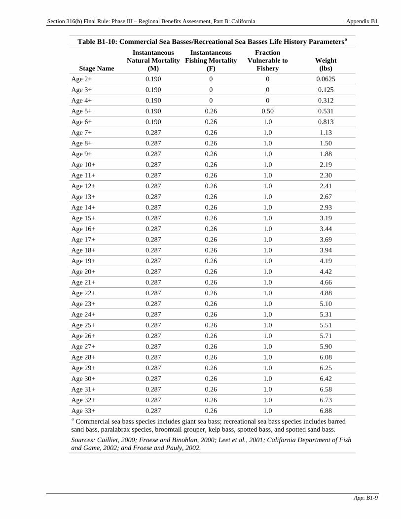
Section 316(b) Final Rule: Phase III – Regional Benefits Assessment, Part B: California Appendix B1
App. B1-9
Table B1-10: Commercial Sea Basses/Recreational Sea Basses Life History ParametersP
aP
Stage Name
Instantaneous Natural Mortality
(M)
Instantaneous Fishing Mortality
(F)
Fraction Vulnerable to
Fishery Weight
(lbs) Age 2+ 0.190 0 0 0.0625 Age 3+ 0.190 0 0 0.125 Age 4+ 0.190 0 0 0.312 Age 5+ 0.190 0.26 0.50 0.531 Age 6+ 0.190 0.26 1.0 0.813 Age 7+ 0.287 0.26 1.0 1.13 Age 8+ 0.287 0.26 1.0 1.50 Age 9+ 0.287 0.26 1.0 1.88 Age 10+ 0.287 0.26 1.0 2.19 Age 11+ 0.287 0.26 1.0 2.30 Age 12+ 0.287 0.26 1.0 2.41 Age 13+ 0.287 0.26 1.0 2.67 Age 14+ 0.287 0.26 1.0 2.93 Age 15+ 0.287 0.26 1.0 3.19 Age 16+ 0.287 0.26 1.0 3.44 Age 17+ 0.287 0.26 1.0 3.69 Age 18+ 0.287 0.26 1.0 3.94 Age 19+ 0.287 0.26 1.0 4.19 Age 20+ 0.287 0.26 1.0 4.42 Age 21+ 0.287 0.26 1.0 4.66 Age 22+ 0.287 0.26 1.0 4.88 Age 23+ 0.287 0.26 1.0 5.10 Age 24+ 0.287 0.26 1.0 5.31 Age 25+ 0.287 0.26 1.0 5.51 Age 26+ 0.287 0.26 1.0 5.71 Age 27+ 0.287 0.26 1.0 5.90 Age 28+ 0.287 0.26 1.0 6.08 Age 29+ 0.287 0.26 1.0 6.25 Age 30+ 0.287 0.26 1.0 6.42 Age 31+ 0.287 0.26 1.0 6.58 Age 32+ 0.287 0.26 1.0 6.73 Age 33+ 0.287 0.26 1.0 6.88 P
aP Commercial sea bass species includes giant sea bass; recreational sea bass species includes barred
sand bass, paralabrax species, broomtail grouper, kelp bass, spotted bass, and spotted sand bass. Sources: Cailliet, 2000; Froese and Binohlan, 2000; Leet et al., 2001; California Department of Fish and Game, 2002; and Froese and Pauly, 2002.
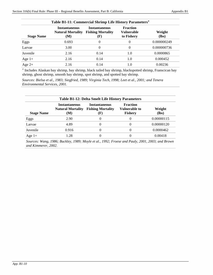
Section 316(b) Final Rule: Phase III – Regional Benefits Assessment, Part B: California Appendix B1
App. B1-10
Table B1-11: Commercial Shrimp Life History ParametersP
aP
Stage Name
Instantaneous Natural Mortality
(M)
Instantaneous Fishing Mortality
(F)
Fraction Vulnerable to Fishery
Weight (lbs)
Eggs 0.693 0 0 0.000000249 Larvae 3.00 0 0 0.000000736 Juvenile 2.16 0.14 1.0 0.0000865 Age 1+ 2.16 0.14 1.0 0.000452 Age 2+ 2.16 0.14 1.0 0.00236 P
aP Includes Alaskan bay shrimp, bay shrimp, black tailed bay shrimp, blackspotted shrimp, Franscican bay
shrimp, ghost shrimp, smooth bay shrimp, spot shrimp, and spotted bay shrimp. Sources: Bielsa et al., 1983; Siegfried, 1989; Virginia Tech, 1998; Leet et al., 2001; and Tenera Environmental Services, 2001.
Table B1-12: Delta Smelt Life History Parameters
Stage Name
Instantaneous Natural Mortality
(M)
Instantaneous Fishing Mortality
(F)
Fraction Vulnerable to
Fishery Weight
(lbs) Eggs 2.90 0 0 0.00000115 Larvae 4.89 0 0 0.00000120 Juvenile 0.916 0 0 0.0000462 Age 1+ 1.28 0 0 0.00418 Sources: Wang, 1986; Buckley, 1989; Moyle et al., 1992; Froese and Pauly, 2001, 2003; and Brown and Kimmerer, 2002.

Section 316(b) Final Rule: Phase III – Regional Benefits Assessment, Part B: California Appendix B1
App. B1-11
Table B1-13: Drums/Croakers Life History ParametersP
aP
Stage Name
Instantaneous Natural Mortality
(M)
Instantaneous Fishing Mortality
(F)
Fraction Vulnerable to Fishery
Weight (lbs)
Eggs 0.500 0 0 0.000000722 Larvae 4.61 0 0 0.00000464 Juvenile 3.38 0 0 0.000212 Age 1+ 0.420 0 0 0.120 Age 2+ 0.420 0 0 0.156 Age 3+ 0.210 0.21 0.50 0.195 Age 4+ 0.210 0.21 1.0 0.239 Age 5+ 0.210 0.21 1.0 0.287 Age 6+ 0.210 0.21 1.0 0.340 Age 7+ 0.210 0.21 1.0 0.398 Age 8+ 0.10 0.21 1.0 0.458 Age 9+ 0.210 0.21 1.0 0.519 Age 10+ 0.210 0.21 1.0 0.584 Age 11+ 0.210 0.21 1.0 0.648 Age 12+ 0.210 0.21 1.0 0.723 P
aP Includes black croaker, California corbina, queenfish, spotfin croaker, white croaker, white
seabass, yellowfin croaker, and other drums or croakers not identified to species. Sources: TIsaacson, 1964; Tenera Environmental Services, 1988, 2000b, 2001; and Cailliet, 2000T.
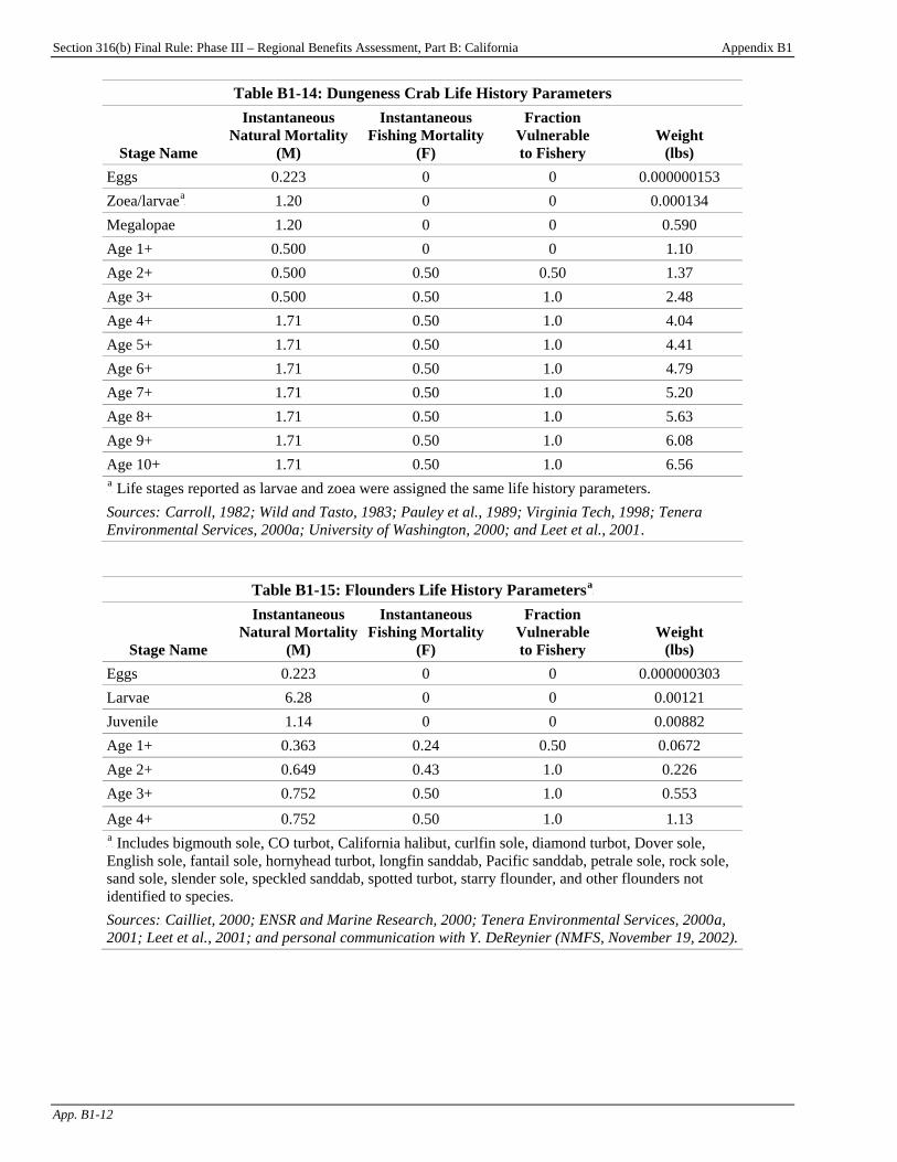
Section 316(b) Final Rule: Phase III – Regional Benefits Assessment, Part B: California Appendix B1
App. B1-12
Table B1-14: Dungeness Crab Life History Parameters
Stage Name
Instantaneous Natural Mortality
(M)
Instantaneous Fishing Mortality
(F)
Fraction Vulnerable to Fishery
Weight (lbs)
Eggs 0.223 0 0 0.000000153 Zoea/larvaeP
aP 1.20 0 0 0.000134
Megalopae 1.20 0 0 0.590 Age 1+ 0.500 0 0 1.10 Age 2+ 0.500 0.50 0.50 1.37 Age 3+ 0.500 0.50 1.0 2.48 Age 4+ 1.71 0.50 1.0 4.04 Age 5+ 1.71 0.50 1.0 4.41 Age 6+ 1.71 0.50 1.0 4.79 Age 7+ 1.71 0.50 1.0 5.20 Age 8+ 1.71 0.50 1.0 5.63 Age 9+ 1.71 0.50 1.0 6.08 Age 10+ 1.71 0.50 1.0 6.56 P
aP Life stages reported as larvae and zoea were assigned the same life history parameters.
Sources: TCarroll, 1982; Wild and Tasto, 1983; Pauley et al., 1989; Virginia Tech, 1998; Tenera Environmental Services, 2000a; University of Washington, 2000; and Leet et al., 2001T.
Table B1-15: Flounders Life History ParametersP
aP
Stage Name
Instantaneous Natural Mortality
(M)
Instantaneous Fishing Mortality
(F)
Fraction Vulnerable to Fishery
Weight (lbs)
Eggs 0.223 0 0 0.000000303 Larvae 6.28 0 0 0.00121 Juvenile 1.14 0 0 0.00882 Age 1+ 0.363 0.24 0.50 0.0672 Age 2+ 0.649 0.43 1.0 0.226 Age 3+ 0.752 0.50 1.0 0.553
Age 4+ 0.752 0.50 1.0 1.13 P
aP Includes bigmouth sole, CO turbot, California halibut, curlfin sole, diamond turbot, Dover sole,
English sole, fantail sole, hornyhead turbot, longfin sanddab, Pacific sanddab, petrale sole, rock sole, sand sole, slender sole, speckled sanddab, spotted turbot, starry flounder, and other flounders not identified to species. Sources:T Cailliet, 2000; ENSR and Marine Research, 2000; Tenera Environmental Services, 2000Ta, 2001; Leet et al., 2001; and personal communication with Y. DeReynier (NMFS, November 19, 2002).

Section 316(b) Final Rule: Phase III – Regional Benefits Assessment, Part B: California Appendix B1
App. B1-13
Table B1-16: Forage Shrimp Life History ParametersP
aP
Stage Name
Instantaneous Natural Mortality
(M)
Instantaneous Fishing Mortality
(F)
Fraction Vulnerable to Fishery
Weight (lbs)
Eggs 0.693 0 0 0.000000249 Larvae 3.00 0 0 0.000000736 Juvenile 2.30 0 0 0.0000865 Age 1+ 2.30 0 0 0.000131 Age 2+ 2.30 0 0 0.00236 P
aP Includes anemone shrimp, blue mud shrimp, broken back shrimp, brown shrimp, California green
shrimp, dock shrimp, mysids, opossum shrimp, oriental shrimp, pistol shrimp, sidestriped shrimp, skeleton shrimp, stout bodied shrimp, striped shrimp, tidepool shrimp, twistclaw pistol shrimp, and other shrimp not identified to species. Sources: Siegfried, 1989; Virginia Tech, 1998; and Tenera Environmental Services, 2001.
Table B1-17: Gobies Life History ParametersP
aP
Stage Name
Instantaneous Natural Mortality
(M)
Instantaneous Fishing Mortality
(F)
Fraction Vulnerable to Fishery
Weight (lbs)
Eggs 0 0 0 0.0000115 Larvae 5.77 0 0 0.0000190 Juvenile 0.871 0 0 0.000169 Age 1+ 1.10 0 0 0.00194 Age 2+ 1.10 0 0 0.00414 Age 3+ 1.10 0 0 0.00763 Age 4+ 1.10 0 0 0.0310 Age 5+ 1.10 0 0 0.0810 P
aP Includes arrow goby, bay goby, blackeye goby, blind goby, chameleon goby, cheekspot goby,
longjaw mudsucker shadow goby, yellowfin goby, and other gobies not identified to species. Sources: Wang, 1986; Froese and Pauly, 2000, 2002; Tenera Environmental Services, 2000a; and NMFS, 2003a.
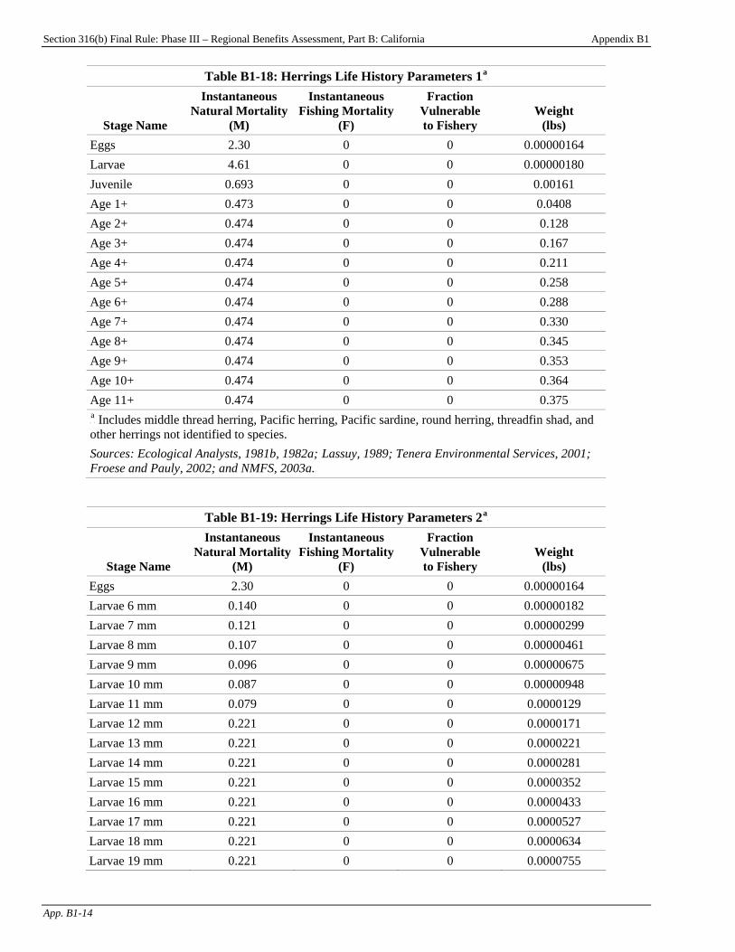
Section 316(b) Final Rule: Phase III – Regional Benefits Assessment, Part B: California Appendix B1
App. B1-14
Table B1-18: Herrings Life History Parameters 1P
aP
Stage Name
Instantaneous Natural Mortality
(M)
Instantaneous Fishing Mortality
(F)
Fraction Vulnerable to Fishery
Weight (lbs)
Eggs 2.30 0 0 0.00000164 Larvae 4.61 0 0 0.00000180 Juvenile 0.693 0 0 0.00161 Age 1+ 0.473 0 0 0.0408 Age 2+ 0.474 0 0 0.128 Age 3+ 0.474 0 0 0.167 Age 4+ 0.474 0 0 0.211 Age 5+ 0.474 0 0 0.258 Age 6+ 0.474 0 0 0.288 Age 7+ 0.474 0 0 0.330 Age 8+ 0.474 0 0 0.345 Age 9+ 0.474 0 0 0.353 Age 10+ 0.474 0 0 0.364 Age 11+ 0.474 0 0 0.375 P
aP Includes middle thread herring, Pacific herring, Pacific sardine, round herring, threadfin shad, and
other herrings not identified to species. Sources: Ecological Analysts, 1981b, 1982a; TLassuy, 1989; Tenera Environmental Services, 2001; Froese and Pauly, 2002; and NMFS, 2003a.T
Table B1-19: Herrings Life History Parameters 2P
aP
Stage Name
Instantaneous Natural Mortality
(M)
Instantaneous Fishing Mortality
(F)
Fraction Vulnerable to Fishery
Weight (lbs)
Eggs 2.30 0 0 0.00000164 Larvae 6 mm 0.140 0 0 0.00000182 Larvae 7 mm 0.121 0 0 0.00000299 Larvae 8 mm 0.107 0 0 0.00000461 Larvae 9 mm 0.096 0 0 0.00000675 Larvae 10 mm 0.087 0 0 0.00000948 Larvae 11 mm 0.079 0 0 0.0000129 Larvae 12 mm 0.221 0 0 0.0000171 Larvae 13 mm 0.221 0 0 0.0000221 Larvae 14 mm 0.221 0 0 0.0000281 Larvae 15 mm 0.221 0 0 0.0000352 Larvae 16 mm 0.221 0 0 0.0000433 Larvae 17 mm 0.221 0 0 0.0000527 Larvae 18 mm 0.221 0 0 0.0000634 Larvae 19 mm 0.221 0 0 0.0000755
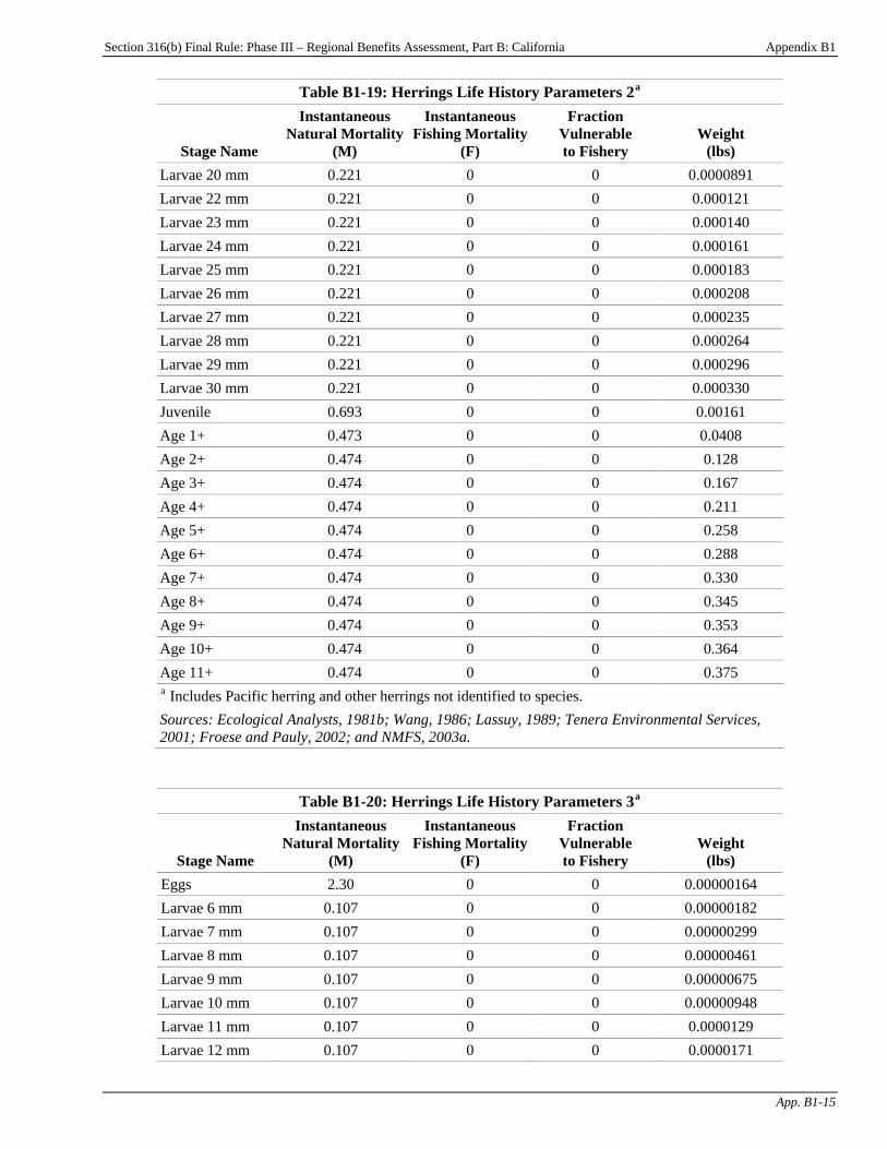
Section 316(b) Final Rule: Phase III – Regional Benefits Assessment, Part B: California Appendix B1
App. B1-15
Table B1-19: Herrings Life History Parameters 2P
aP
Stage Name
Instantaneous Natural Mortality
(M)
Instantaneous Fishing Mortality
(F)
Fraction Vulnerable to Fishery
Weight (lbs)
Larvae 20 mm 0.221 0 0 0.0000891 Larvae 22 mm 0.221 0 0 0.000121 Larvae 23 mm 0.221 0 0 0.000140 Larvae 24 mm 0.221 0 0 0.000161 Larvae 25 mm 0.221 0 0 0.000183 Larvae 26 mm 0.221 0 0 0.000208 Larvae 27 mm 0.221 0 0 0.000235 Larvae 28 mm 0.221 0 0 0.000264 Larvae 29 mm 0.221 0 0 0.000296 Larvae 30 mm 0.221 0 0 0.000330 Juvenile 0.693 0 0 0.00161 Age 1+ 0.473 0 0 0.0408 Age 2+ 0.474 0 0 0.128 Age 3+ 0.474 0 0 0.167 Age 4+ 0.474 0 0 0.211 Age 5+ 0.474 0 0 0.258 Age 6+ 0.474 0 0 0.288 Age 7+ 0.474 0 0 0.330 Age 8+ 0.474 0 0 0.345 Age 9+ 0.474 0 0 0.353 Age 10+ 0.474 0 0 0.364 Age 11+ 0.474 0 0 0.375 P
aP Includes Pacific herring and other herrings not identified to species.
Sources: Ecological Analysts, 1981b; Wang, 1986; Lassuy, 1989; Tenera Environmental Services, 2001; Froese and Pauly, 2002; and NMFS, 2003a.
Table B1-20: Herrings Life History Parameters 3P
aP
Stage Name
Instantaneous Natural Mortality
(M)
Instantaneous Fishing Mortality
(F)
Fraction Vulnerable to Fishery
Weight (lbs)
Eggs 2.30 0 0 0.00000164 Larvae 6 mm 0.107 0 0 0.00000182 Larvae 7 mm 0.107 0 0 0.00000299 Larvae 8 mm 0.107 0 0 0.00000461 Larvae 9 mm 0.107 0 0 0.00000675 Larvae 10 mm 0.107 0 0 0.00000948 Larvae 11 mm 0.107 0 0 0.0000129 Larvae 12 mm 0.107 0 0 0.0000171
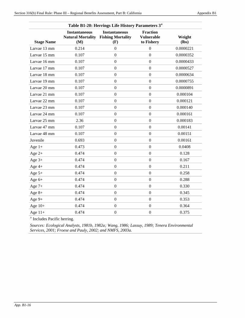
Section 316(b) Final Rule: Phase III – Regional Benefits Assessment, Part B: California Appendix B1
App. B1-16
Table B1-20: Herrings Life History Parameters 3P
aP
Stage Name
Instantaneous Natural Mortality
(M)
Instantaneous Fishing Mortality
(F)
Fraction Vulnerable to Fishery
Weight (lbs)
Larvae 13 mm 0.214 0 0 0.0000221 Larvae 15 mm 0.107 0 0 0.0000352 Larvae 16 mm 0.107 0 0 0.0000433 Larvae 17 mm 0.107 0 0 0.0000527 Larvae 18 mm 0.107 0 0 0.0000634 Larvae 19 mm 0.107 0 0 0.0000755 Larvae 20 mm 0.107 0 0 0.0000891 Larvae 21 mm 0.107 0 0 0.000104 Larvae 22 mm 0.107 0 0 0.000121 Larvae 23 mm 0.107 0 0 0.000140 Larvae 24 mm 0.107 0 0 0.000161 Larvae 25 mm 2.36 0 0 0.000183 Larvae 47 mm 0.107 0 0 0.00141 Larvae 48 mm 0.107 0 0 0.00151 Juvenile 0.693 0 0 0.00161 Age 1+ 0.473 0 0 0.0408 Age 2+ 0.474 0 0 0.128 Age 3+ 0.474 0 0 0.167 Age 4+ 0.474 0 0 0.211 Age 5+ 0.474 0 0 0.258 Age 6+ 0.474 0 0 0.288 Age 7+ 0.474 0 0 0.330 Age 8+ 0.474 0 0 0.345 Age 9+ 0.474 0 0 0.353 Age 10+ 0.474 0 0 0.364 Age 11+ 0.474 0 0 0.375 P
aP Includes Pacific herring.
Sources: TEcological Analysts, 1981b, 1982aT; Wang, 1986; Lassuy, 1989; Tenera Environmental Services, 2001; Froese and Pauly, 2002; and NMFS, 2003a.
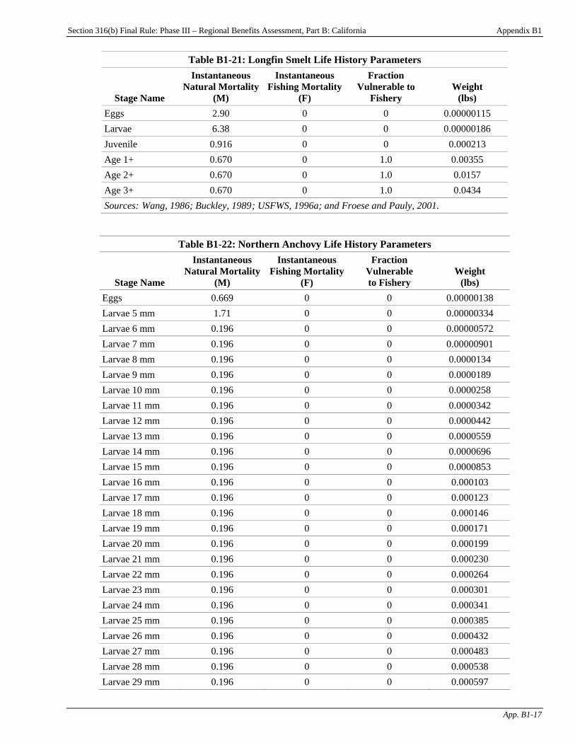
Section 316(b) Final Rule: Phase III – Regional Benefits Assessment, Part B: California Appendix B1
App. B1-17
Table B1-21: Longfin Smelt Life History Parameters
Stage Name
Instantaneous Natural Mortality
(M)
Instantaneous Fishing Mortality
(F)
Fraction Vulnerable to
Fishery Weight
(lbs) Eggs 2.90 0 0 0.00000115 Larvae 6.38 0 0 0.00000186 Juvenile 0.916 0 0 0.000213 Age 1+ 0.670 0 1.0 0.00355 Age 2+ 0.670 0 1.0 0.0157 Age 3+ 0.670 0 1.0 0.0434 Sources:T Wang, 1986; Buckley, 1989T; USFWS, 1996a; and Froese and Pauly, 2001.
Table B1-22: Northern Anchovy Life History Parameters
Stage Name
Instantaneous Natural Mortality
(M)
Instantaneous Fishing Mortality
(F)
Fraction Vulnerable to Fishery
Weight (lbs)
Eggs 0.669 0 0 0.00000138 Larvae 5 mm 1.71 0 0 0.00000334 Larvae 6 mm 0.196 0 0 0.00000572 Larvae 7 mm 0.196 0 0 0.00000901 Larvae 8 mm 0.196 0 0 0.0000134 Larvae 9 mm 0.196 0 0 0.0000189 Larvae 10 mm 0.196 0 0 0.0000258 Larvae 11 mm 0.196 0 0 0.0000342 Larvae 12 mm 0.196 0 0 0.0000442 Larvae 13 mm 0.196 0 0 0.0000559 Larvae 14 mm 0.196 0 0 0.0000696 Larvae 15 mm 0.196 0 0 0.0000853 Larvae 16 mm 0.196 0 0 0.000103 Larvae 17 mm 0.196 0 0 0.000123 Larvae 18 mm 0.196 0 0 0.000146 Larvae 19 mm 0.196 0 0 0.000171 Larvae 20 mm 0.196 0 0 0.000199 Larvae 21 mm 0.196 0 0 0.000230 Larvae 22 mm 0.196 0 0 0.000264 Larvae 23 mm 0.196 0 0 0.000301 Larvae 24 mm 0.196 0 0 0.000341 Larvae 25 mm 0.196 0 0 0.000385 Larvae 26 mm 0.196 0 0 0.000432 Larvae 27 mm 0.196 0 0 0.000483 Larvae 28 mm 0.196 0 0 0.000538 Larvae 29 mm 0.196 0 0 0.000597
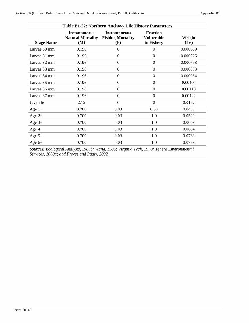
Section 316(b) Final Rule: Phase III – Regional Benefits Assessment, Part B: California Appendix B1
App. B1-18
Table B1-22: Northern Anchovy Life History Parameters
Stage Name
Instantaneous Natural Mortality
(M)
Instantaneous Fishing Mortality
(F)
Fraction Vulnerable to Fishery
Weight (lbs)
Larvae 30 mm 0.196 0 0 0.000659 Larvae 31 mm 0.196 0 0 0.000726 Larvae 32 mm 0.196 0 0 0.000798 Larvae 33 mm 0.196 0 0 0.000873 Larvae 34 mm 0.196 0 0 0.000954 Larvae 35 mm 0.196 0 0 0.00104 Larvae 36 mm 0.196 0 0 0.00113 Larvae 37 mm 0.196 0 0 0.00122 Juvenile 2.12 0 0 0.0132 Age 1+ 0.700 0.03 0.50 0.0408 Age 2+ 0.700 0.03 1.0 0.0529 Age 3+ 0.700 0.03 1.0 0.0609 Age 4+ 0.700 0.03 1.0 0.0684 Age 5+ 0.700 0.03 1.0 0.0763 Age 6+ 0.700 0.03 1.0 0.0789 Sources: Ecological Analysts, 1980b; Wang, 1986; Virginia Tech, 1998; Tenera Environmental Services, 2000a; and Froese and Pauly, 2002.
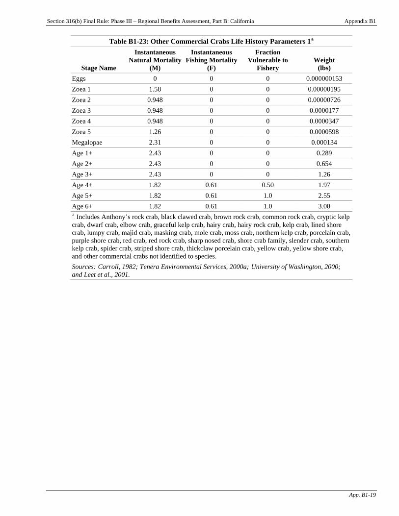
Section 316(b) Final Rule: Phase III – Regional Benefits Assessment, Part B: California Appendix B1
App. B1-19
Table B1-23: Other Commercial Crabs Life History Parameters 1P
aP
Stage Name
Instantaneous Natural Mortality
(M)
Instantaneous Fishing Mortality
(F)
Fraction Vulnerable to
Fishery Weight
(lbs) Eggs 0 0 0 0.000000153 Zoea 1 1.58 0 0 0.00000195 Zoea 2 0.948 0 0 0.00000726 Zoea 3 0.948 0 0 0.0000177 Zoea 4 0.948 0 0 0.0000347 Zoea 5 1.26 0 0 0.0000598 Megalopae 2.31 0 0 0.000134 Age 1+ 2.43 0 0 0.289 Age 2+ 2.43 0 0 0.654 Age 3+ 2.43 0 0 1.26 Age 4+ 1.82 0.61 0.50 1.97 Age 5+ 1.82 0.61 1.0 2.55 Age 6+ 1.82 0.61 1.0 3.00 P
aP Includes Anthony’s rock crab, black clawed crab, brown rock crab, common rock crab, cryptic kelp
crab, dwarf crab, elbow crab, graceful kelp crab, hairy crab, hairy rock crab, kelp crab, lined shore crab, lumpy crab, majid crab, masking crab, mole crab, moss crab, northern kelp crab, porcelain crab, purple shore crab, red crab, red rock crab, sharp nosed crab, shore crab family, slender crab, southern kelp crab, spider crab, striped shore crab, thickclaw porcelain crab, yellow crab, yellow shore crab, and other commercial crabs not identified to species. Sources: TCarroll, 1982; Tenera Environmental Services, 2000a; TUniversity of Washington, 2000; and Leet et al., 2001.
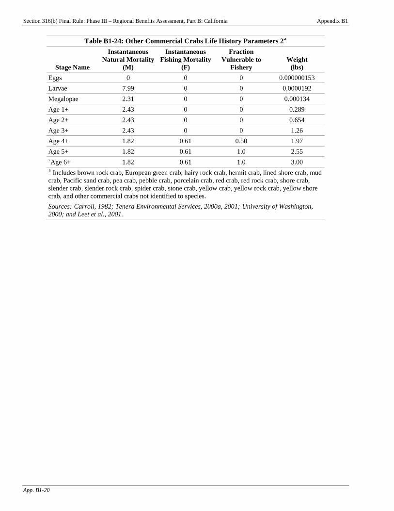
Section 316(b) Final Rule: Phase III – Regional Benefits Assessment, Part B: California Appendix B1
App. B1-20
Table B1-24: Other Commercial Crabs Life History Parameters 2P
aP
Stage Name
Instantaneous Natural Mortality
(M)
Instantaneous Fishing Mortality
(F)
Fraction Vulnerable to
Fishery Weight
(lbs) Eggs 0 0 0 0.000000153 Larvae 7.99 0 0 0.0000192 Megalopae 2.31 0 0 0.000134 Age 1+ 2.43 0 0 0.289 Age 2+ 2.43 0 0 0.654 Age 3+ 2.43 0 0 1.26 Age 4+ 1.82 0.61 0.50 1.97 Age 5+ 1.82 0.61 1.0 2.55 `Age 6+ 1.82 0.61 1.0 3.00 P
aP Includes brown rock crab, European green crab, hairy rock crab, hermit crab, lined shore crab, mud
crab, Pacific sand crab, pea crab, pebble crab, porcelain crab, red crab, red rock crab, shore crab, slender crab, slender rock crab, spider crab, stone crab, yellow crab, yellow rock crab, yellow shore crab, and other commercial crabs not identified to species. Sources: TCarroll, 1982; Tenera Environmental Services, 2000a, 2001; TUniversity of Washington, 2000; and Leet et al., 2001.
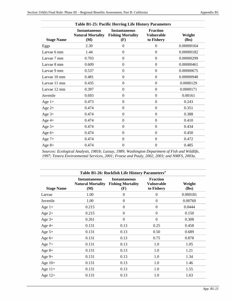
Section 316(b) Final Rule: Phase III – Regional Benefits Assessment, Part B: California Appendix B1
App. B1-21
Table B1-25: Pacific Herring Life History Parameters
Stage Name
Instantaneous Natural Mortality
(M)
Instantaneous Fishing Mortality
(F)
Fraction Vulnerable to Fishery
Weight (lbs)
Eggs 2.30 0 0 0.00000164 Larvae 6 mm 1.44 0 0 0.00000182 Larvae 7 mm 0.703 0 0 0.00000299 Larvae 8 mm 0.609 0 0 0.00000461 Larvae 9 mm 0.537 0 0 0.00000675 Larvae 10 mm 0.481 0 0 0.00000948 Larvae 11 mm 0.435 0 0 0.0000129 Larvae 12 mm 0.397 0 0 0.0000171 Juvenile 0.693 0 0 0.00161 Age 1+ 0.473 0 0 0.243 Age 2+ 0.474 0 0 0.351 Age 3+ 0.474 0 0 0.388 Age 4+ 0.474 0 0 0.410 Age 5+ 0.474 0 0 0.434 Age 6+ 0.474 0 0 0.450 Age 7+ 0.474 0 0 0.472 Age 8+ 0.474 0 0 0.485 Sources: Ecological Analysts, 1981b; Lassuy, 1989; Washington Department of Fish and Wildlife, 1997; Tenera Environmental Services, 2001; Froese and Pauly, 2002, 2003; and NMFS, 2003a.
Table B1-26: Rockfish Life History ParametersP
aP
Stage Name
Instantaneous Natural Mortality
(M)
Instantaneous Fishing Mortality
(F)
Fraction Vulnerable to Fishery
Weight (lbs)
Larvae 1.00 0 0 0.000181 Juvenile 1.00 0 0 0.00760 Age 1+ 0.215 0 0 0.0444 Age 2+ 0.215 0 0 0.150 Age 3+ 0.261 0 0 0.308 Age 4+ 0.131 0.13 0.25 0.458 Age 5+ 0.131 0.13 0.50 0.689 Age 6+ 0.131 0.13 0.75 0.878 Age 7+ 0.131 0.13 1.0 1.05 Age 8+ 0.131 0.13 1.0 1.21 Age 9+ 0.131 0.13 1.0 1.34 Age 10+ 0.131 0.13 1.0 1.46 Age 11+ 0.131 0.13 1.0 1.55 Age 12+ 0.131 0.13 1.0 1.63
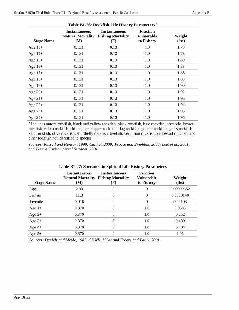
Section 316(b) Final Rule: Phase III – Regional Benefits Assessment, Part B: California Appendix B1
App. B1-22
Table B1-26: Rockfish Life History ParametersP
aP
Stage Name
Instantaneous Natural Mortality
(M)
Instantaneous Fishing Mortality
(F)
Fraction Vulnerable to Fishery
Weight (lbs)
Age 13+ 0.131 0.13 1.0 1.70 Age 14+ 0.131 0.13 1.0 1.75 Age 15+ 0.131 0.13 1.0 1.80 Age 16+ 0.131 0.13 1.0 1.83 Age 17+ 0.131 0.13 1.0 1.86 Age 18+ 0.131 0.13 1.0 1.88 Age 19+ 0.131 0.13 1.0 1.90 Age 20+ 0.131 0.13 1.0 1.92 Age 21+ 0.131 0.13 1.0 1.93 Age 22+ 0.131 0.13 1.0 1.94 Age 23+ 0.131 0.13 1.0 1.95 Age 24+ 0.131 0.13 1.0 1.95 P
aP Includes aurora rockfish, black and yellow rockfish, black rockfish, blue rockfish, bocaccio, brown
rockfish, calico rockfish, chilipepper, copper rockfish, flag rockfish, gopher rockfish, grass rockfish, kelp rockfish, olive rockfish, shortbelly rockfish, treefish, vermilion rockfish, yellowtail rockfish, and other rockfish not identified to species. Sources: Russell and Hanson, 1990; Cailliet, 2000; TFroese and Binohlan, 2000; Leet et al., 2001; and Tenera Environmental Services, 2001T.
Table B1-27: Sacramento Splittail Life History Parameters
Stage Name
Instantaneous Natural Mortality
(M)
Instantaneous Fishing Mortality
(F)
Fraction Vulnerable to Fishery
Weight (lbs)
Eggs 2.30 0 0 0.00000352 Larvae 11.3 0 0 0.0000140 Juvenile 0.916 0 0 0.00103 Age 1+ 0.370 0 1.0 0.0683 Age 2+ 0.370 0 1.0 0.252 Age 3+ 0.370 0 1.0 0.480 Age 4+ 0.370 0 1.0 0.704 Age 5+ 0.370 0 1.0 1.05 Sources: Daniels and Moyle, 1983; CDWR, 1994; and Froese and Pauly, 2001.
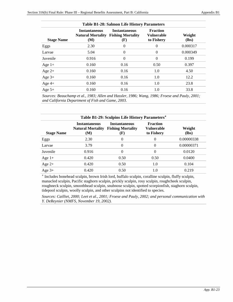
Section 316(b) Final Rule: Phase III – Regional Benefits Assessment, Part B: California Appendix B1
App. B1-23
Table B1-28: Salmon Life History Parameters
Stage Name
Instantaneous Natural Mortality
(M)
Instantaneous Fishing Mortality
(F)
Fraction Vulnerable to Fishery
Weight (lbs)
Eggs 2.30 0 0 0.000317 Larvae 5.04 0 0 0.000349 Juvenile 0.916 0 0 0.199 Age 1+ 0.160 0.16 0.50 0.397 Age 2+ 0.160 0.16 1.0 4.50 Age 3+ 0.160 0.16 1.0 12.2 Age 4+ 0.160 0.16 1.0 23.8 Age 5+ 0.160 0.16 1.0 33.8 Sources: Beauchamp et al., 1983; Allen and Hassler, 1986; Wang, 1986; Froese and Pauly, 2001; and California Department of Fish and Game, 2003.
Table B1-29: Sculpins Life History ParametersP
aP
Stage Name
Instantaneous Natural Mortality
(M)
Instantaneous Fishing Mortality
(F)
Fraction Vulnerable to Fishery
Weight (lbs)
Eggs 2.30 0 0 0.00000338 Larvae 3.79 0 0 0.00000371 Juvenile 0.916 0 0 0.0120 Age 1+ 0.420 0.50 0.50 0.0400 Age 2+ 0.420 0.50 1.0 0.104 Age 3+ 0.420 0.50 1.0 0.219 P
aP Includes bonehead sculpin, brown Irish lord, buffalo sculpin, coralline sculpin, fluffy sculpin,
manacled sculpin, Pacific staghorn sculpin, prickly sculpin, rosy sculpin, roughcheek sculpin, roughneck sculpin, smoothhead sculpin, snubnose sculpin, spotted scorpionfish, staghorn sculpin, tidepool sculpin, woolly sculpin, and other sculpins not identified to species. Sources: Cailliet, 2000; Leet et al., 2001; Froese and Pauly, 2002; and personal communication with Y. DeReynier (NMFS, November 19, 2002).
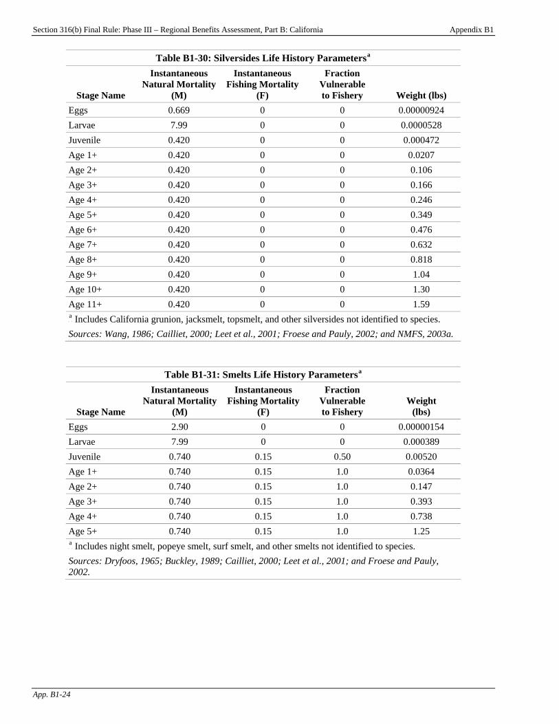
Section 316(b) Final Rule: Phase III – Regional Benefits Assessment, Part B: California Appendix B1
App. B1-24
Table B1-30: Silversides Life History ParametersP
aP
Stage Name
Instantaneous Natural Mortality
(M)
Instantaneous Fishing Mortality
(F)
Fraction Vulnerable to Fishery Weight (lbs)
Eggs 0.669 0 0 0.00000924 Larvae 7.99 0 0 0.0000528 Juvenile 0.420 0 0 0.000472 Age 1+ 0.420 0 0 0.0207 Age 2+ 0.420 0 0 0.106 Age 3+ 0.420 0 0 0.166 Age 4+ 0.420 0 0 0.246 Age 5+ 0.420 0 0 0.349 Age 6+ 0.420 0 0 0.476 Age 7+ 0.420 0 0 0.632 Age 8+ 0.420 0 0 0.818 Age 9+ 0.420 0 0 1.04 Age 10+ 0.420 0 0 1.30 Age 11+ 0.420 0 0 1.59 P
aP Includes California grunion, jacksmelt, topsmelt, and other silversides not identified to species.
Sources: Wang, 1986; Cailliet, 2000; Leet et al., 2001; Froese and Pauly, 2002; and NMFS, 2003a.
Table B1-31: Smelts Life History ParametersP
aP
Stage Name
Instantaneous Natural Mortality
(M)
Instantaneous Fishing Mortality
(F)
Fraction Vulnerable to Fishery
Weight (lbs)
Eggs 2.90 0 0 0.00000154 Larvae 7.99 0 0 0.000389 Juvenile 0.740 0.15 0.50 0.00520 Age 1+ 0.740 0.15 1.0 0.0364 Age 2+ 0.740 0.15 1.0 0.147 Age 3+ 0.740 0.15 1.0 0.393 Age 4+ 0.740 0.15 1.0 0.738 Age 5+ 0.740 0.15 1.0 1.25 P
aP Includes night smelt, popeye smelt, surf smelt, and other smelts not identified to species.
Sources: Dryfoos, 1965; Buckley, 1989; Cailliet, 2000; Leet et al., 2001; and Froese and Pauly, 2002.
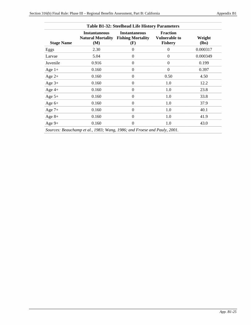
Section 316(b) Final Rule: Phase III – Regional Benefits Assessment, Part B: California Appendix B1
App. B1-25
Table B1-32: Steelhead Life History Parameters
Stage Name
Instantaneous Natural Mortality
(M)
Instantaneous Fishing Mortality
(F)
Fraction Vulnerable to
Fishery Weight
(lbs) Eggs 2.30 0 0 0.000317 Larvae 5.04 0 0 0.000349 Juvenile 0.916 0 0 0.199 Age 1+ 0.160 0 0 0.397 Age 2+ 0.160 0 0.50 4.50 Age 3+ 0.160 0 1.0 12.2 Age 4+ 0.160 0 1.0 23.8 Age 5+ 0.160 0 1.0 33.8 Age 6+ 0.160 0 1.0 37.9 Age 7+ 0.160 0 1.0 40.1 Age 8+ 0.160 0 1.0 41.9 Age 9+ 0.160 0 1.0 43.0 Sources: Beauchamp et al., 1983; Wang, 1986; and Froese and Pauly, 2001.
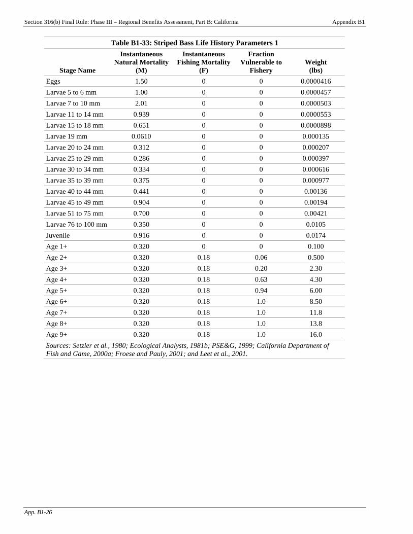
Section 316(b) Final Rule: Phase III – Regional Benefits Assessment, Part B: California Appendix B1
App. B1-26
Table B1-33: Striped Bass Life History Parameters 1
Stage Name
Instantaneous Natural Mortality
(M)
Instantaneous Fishing Mortality
(F)
Fraction Vulnerable to
Fishery Weight
(lbs) Eggs 1.50 0 0 0.0000416 Larvae 5 to 6 mm 1.00 0 0 0.0000457 Larvae 7 to 10 mm 2.01 0 0 0.0000503 Larvae 11 to 14 mm 0.939 0 0 0.0000553 Larvae 15 to 18 mm 0.651 0 0 0.0000898 Larvae 19 mm 0.0610 0 0 0.000135 Larvae 20 to 24 mm 0.312 0 0 0.000207 Larvae 25 to 29 mm 0.286 0 0 0.000397 Larvae 30 to 34 mm 0.334 0 0 0.000616 Larvae 35 to 39 mm 0.375 0 0 0.000977 Larvae 40 to 44 mm 0.441 0 0 0.00136 Larvae 45 to 49 mm 0.904 0 0 0.00194 Larvae 51 to 75 mm 0.700 0 0 0.00421 Larvae 76 to 100 mm 0.350 0 0 0.0105 Juvenile 0.916 0 0 0.0174 Age 1+ 0.320 0 0 0.100 Age 2+ 0.320 0.18 0.06 0.500 Age 3+ 0.320 0.18 0.20 2.30 Age 4+ 0.320 0.18 0.63 4.30 Age 5+ 0.320 0.18 0.94 6.00 Age 6+ 0.320 0.18 1.0 8.50 Age 7+ 0.320 0.18 1.0 11.8 Age 8+ 0.320 0.18 1.0 13.8 Age 9+ 0.320 0.18 1.0 16.0 Sources: Setzler et al., 1980; Ecological Analysts, 1981b; PSE&G, 1999; California Department of Fish and Game, 2000a; Froese and Pauly, 2001; and Leet et al., 2001.

Section 316(b) Final Rule: Phase III – Regional Benefits Assessment, Part B: California Appendix B1
App. B1-27
Table B1-34: Striped Bass Life History Parameters 2
Stage Name
Instantaneous Natural Mortality
(M)
Instantaneous Fishing Mortality
(F)
Fraction Vulnerable to
Fishery Weight
(lbs) Eggs 1.50 0 0 0.0000416 Larvae 7.44 0 0 0.0000457 Juvenile 0.916 0 0 0.0174 Age 1+ 0.320 0 0 0.100 Age 2+ 0.320 0.18 0.06 0.500 Age 3+ 0.320 0.18 0.20 2.30 Age 4+ 0.320 0.18 0.63 4.30 Age 5+ 0.320 0.18 0.94 6.00 Age 6+ 0.320 0.18 1.0 8.50 Age 7+ 0.320 0.18 1.0 11.8 Age 8+ 0.320 0.18 1.0 13.8 Age 9+ 0.320 0.18 1.0 16.0 Sources: Setzler et al., 1980; Ecological Analysts, 1981b; PSE&G, 1999; California Department of Fish and Game, 2000a; Froese and Pauly, 2001; and Leet et al., 2001.
Table B1-35: Surfperches Life History ParametersP
aP
Stage Name
Instantaneous Natural Mortality
(M)
Instantaneous Fishing Mortality
(F)
Fraction Vulnerable to Fishery
Weight (lbs)
Juvenile 0.560 0 0 0.00443 Age 1+ 0.280 0 0 0.0429 Age 2+ 0.280 0.28 0.50 0.125 Age 3+ 0.280 0.28 1.0 0.203 Age 4+ 0.280 0.28 1.0 0.261 Age 5+ 0.280 0.28 1.0 0.300 Age 6+ 0.280 0.28 1.0 0.324 P
aP Includes barred surfperch, black surfperch, calico surfperch, dwarf surfperch, island surfperch, kelp
surfperch, pile surfperch, pink seaperch, rainbow surfperch, rubberlip surfperch, shiner surfperch, silver surfperch, spotfin surfperch, striped surfperch, walleye surfperch, white seaperch, and other surfperches not identified to species. Sources: Cailliet, 2000; Froese and Binohlan, 2000; Leet et al., 2001; and Froese and Pauly, 2002.
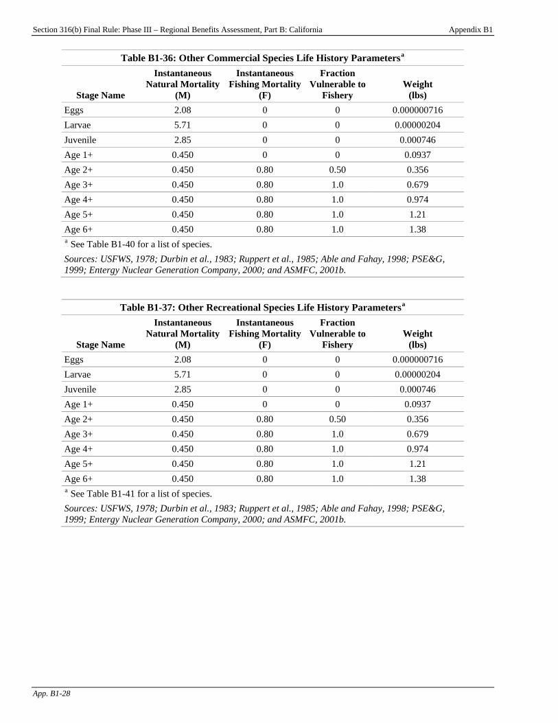
Section 316(b) Final Rule: Phase III – Regional Benefits Assessment, Part B: California Appendix B1
App. B1-28
Table B1-36: Other Commercial Species Life History ParametersP
aP
Stage Name
Instantaneous Natural Mortality
(M)
Instantaneous Fishing Mortality
(F)
Fraction Vulnerable to
Fishery Weight
(lbs) Eggs 2.08 0 0 0.000000716 Larvae 5.71 0 0 0.00000204 Juvenile 2.85 0 0 0.000746 Age 1+ 0.450 0 0 0.0937 Age 2+ 0.450 0.80 0.50 0.356 Age 3+ 0.450 0.80 1.0 0.679 Age 4+ 0.450 0.80 1.0 0.974 Age 5+ 0.450 0.80 1.0 1.21 Age 6+ 0.450 0.80 1.0 1.38 P
aP See Table B1-40 for a list of species.
Sources: USFWS, 1978; Durbin et al., 1983; Ruppert et al., 1985; Able and Fahay, 1998; PSE&G, 1999; Entergy Nuclear Generation Company, 2000; and ASMFC, 2001b.
Table B1-37: Other Recreational Species Life History ParametersP
aP
Stage Name
Instantaneous Natural Mortality
(M)
Instantaneous Fishing Mortality
(F)
Fraction Vulnerable to
Fishery Weight
(lbs) Eggs 2.08 0 0 0.000000716 Larvae 5.71 0 0 0.00000204 Juvenile 2.85 0 0 0.000746 Age 1+ 0.450 0 0 0.0937 Age 2+ 0.450 0.80 0.50 0.356 Age 3+ 0.450 0.80 1.0 0.679 Age 4+ 0.450 0.80 1.0 0.974 Age 5+ 0.450 0.80 1.0 1.21 Age 6+ 0.450 0.80 1.0 1.38 P
aP See Table B1-41 for a list of species.
Sources: USFWS, 1978; Durbin et al., 1983; Ruppert et al., 1985; Able and Fahay, 1998; PSE&G, 1999; Entergy Nuclear Generation Company, 2000; and ASMFC, 2001b.
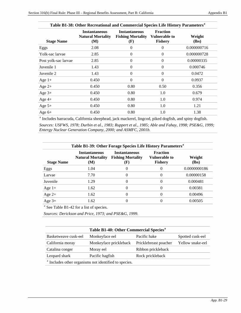
Section 316(b) Final Rule: Phase III – Regional Benefits Assessment, Part B: California Appendix B1
App. B1-29
Table B1-38: Other Recreational and Commercial Species Life History ParametersP
aP
Stage Name
Instantaneous Natural Mortality
(M)
Instantaneous Fishing Mortality
(F)
Fraction Vulnerable to
Fishery Weight
(lbs) Eggs 2.08 0 0 0.000000716 Yolk-sac larvae 2.85 0 0 0.000000728 Post yolk-sac larvae 2.85 0 0 0.00000335 Juvenile 1 1.43 0 0 0.000746 Juvenile 2 1.43 0 0 0.0472 Age 1+ 0.450 0 0 0.0937 Age 2+ 0.450 0.80 0.50 0.356 Age 3+ 0.450 0.80 1.0 0.679 Age 4+ 0.450 0.80 1.0 0.974 Age 5+ 0.450 0.80 1.0 1.21 Age 6+ 0.450 0.80 1.0 1.38 P
aP Includes barracuda, California sheephead, jack mackerel, lingcod, piked dogfish, and spiny dogfish.
Sources: USFWS, 1978; Durbin et al., 1983; Ruppert et al., 1985; Able and Fahay, 1998; PSE&G, 1999; Entergy Nuclear Generation Company, 2000; and ASMFC, 2001b.
Table B1-39: Other Forage Species Life History ParametersP
aP
Stage Name
Instantaneous Natural Mortality
(M)
Instantaneous Fishing Mortality
(F)
Fraction Vulnerable to
Fishery Weight
(lbs) Eggs 1.04 0 0 0.0000000186 Larvae 7.70 0 0 0.00000158 Juvenile 1.29 0 0 0.000481 Age 1+ 1.62 0 0 0.00381 Age 2+ 1.62 0 0 0.00496 Age 3+ 1.62 0 0 0.00505 P
aP See Table B1-42 for a list of species.
Sources: Derickson and Price, 1973; and PSE&G, 1999.
Table B1-40: Other Commercial SpeciesP
aP
Basketweave cusk-eel Monkeyface eel Pacific hake Spotted cusk-eel California moray Monkeyface prickleback Pricklebreast poacher Yellow snake-eel Catalina conger Moray eel Ribbon prickleback Leopard shark Pacific hagfish Rock prickleback P
aP Includes other organisms not identified to species.
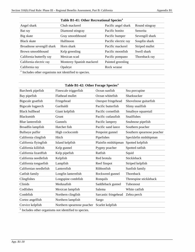
Section 316(b) Final Rule: Phase III – Regional Benefits Assessment, Part B: California Appendix B1
App. B1-30
Table B1-41: Other Recreational SpeciesP
aP
Angel shark Chub mackerel Pacific angel shark Round stingray Bat ray Diamond stingray Pacific bonito Senorita Big skate Gray smoothhound Pacific bumper Sevengill shark Black skate Halfmoon Pacific electric ray Soupfin shark Broadnose sevengill shark Horn shark Pacific mackerel Striped mullet Brown smoothhound Kelp greenling Pacific moonfish Swell shark California butterfly ray Mexican scad Pacific pompano Thornback ray California electric ray Monterey Spanish mackerel Painted greenling California ray Opaleye Rock wrasse P
aP Includes other organisms not identified to species.
Table B1-42: Other Forage SpeciesP
aP
Barcheek pipefish Finescale triggerfish Ocean sunfish Sea porcupine Bay pipefish Flathead mullet Ocean whitefish Sharksucker Bigscale goatfish Fringehead Onespot fringehead Shovelnose guitarfish Bigscale logperch Garibaldi Pacific butterfish Slimy snailfish Black bullhead Giant kelpfish Pacific cornetfish Smalleye squaretail Blacksmith Grunt Pacific cutlassfish Snailfishes Blue lanternfish Gunnels Pacific lamprey Snubnose pipefish Broadfin lampfish Hatchet fish Pacific sand lance Southern poacher Bullseye puffer High cockscomb Penpoint gunnel Southern spearnose poacher California clingfish Hitch Pipefishes Specklefin midshipman California flyingfish Island kelpfish Plainfin midshipman Spotted kelpfish California killifish Kelp gunnel Pygmy poacher Spotted ratfish California lizardfish Kelp pipefish Ratfish Squid California needlefish Kelpfish Red brotula Stickleback California tonguefish Lampfish Reef finspot Striped kelpfish Californian needlefish Lanternfish Ribbonfish Sunfish family Catfish family Longfin lanternfish Rockweed gunnel Thornback Clingfishes Longspine combfish Ronquils Threespine stickleback Clinids Medusafish Saddleback gunnel Tubesnout Codfishes Mexican lampfish Salema White catfish Combfish Northern clingfish Sarcastic fringehead Zebra perch Cortez angelfish Northern lampfish Sargo Crevice kelpfish Northern spearnose poacher Scarlet kelpfish P
aP Includes other organisms not identified to species.
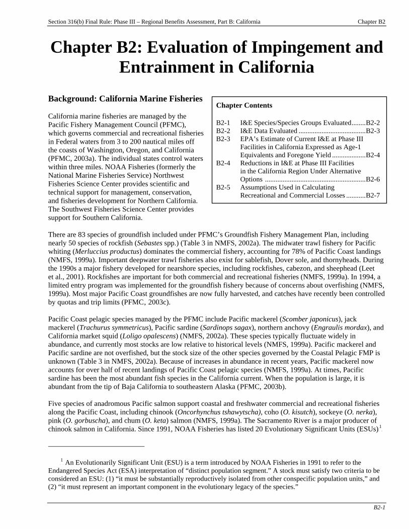
Section 316(b) Final Rule: Phase III – Regional Benefits Assessment, Part B: California Chapter B2
B2-1
Chapter B2: Evaluation of Impingement and Entrainment in California
Background: California Marine Fisheries
Chapter Contents B2-1 I&E Species/Species Groups Evaluated........B2-2 B2-2 I&E Data Evaluated ......................................B2-3 B2-3 EPA’s Estimate of Current I&E at Phase III Facilities in California Expressed as Age-1 Equivalents and Foregone Yield ...................B2-4 B2-4 Reductions in I&E at Phase III Facilities in the California Region Under Alternative Options .........................................................B2-6 B2-5 Assumptions Used in Calculating
Recreational and Commercial Losses ...........B2-7
California marine fisheries are managed by the Pacific Fishery Management Council (PFMC), which governs commercial and recreational fisheries in Federal waters from 3 to 200 nautical miles off the coasts of Washington, Oregon, and California (PFMC, 2003a). The individual states control waters within three miles. NOAA Fisheries (formerly the National Marine Fisheries Service) Northwest Fisheries Science Center provides scientific and technical support for management, conservation, and fisheries development for Northern California. The Southwest Fisheries Science Center provides support for Southern California. There are 83 species of groundfish included under PFMC’s Groundfish Fishery Management Plan, including nearly 50 species of rockfish (Sebastes spp.) (Table 3 in NMFS, 2002a). The midwater trawl fishery for Pacific whiting (Merluccius productus) dominates the commercial fishery, accounting for 78% of Pacific Coast landings (NMFS, 1999a). Important deepwater trawl fisheries also exist for sablefish, Dover sole, and thornyheads. During the 1990s a major fishery developed for nearshore species, including rockfishes, cabezon, and sheephead (Leet et al., 2001). Rockfishes are important for both commercial and recreational fisheries (NMFS, 1999a). In 1994, a limited entry program was implemented for the groundfish fishery because of concerns about overfishing (NMFS, 1999a). Most major Pacific Coast groundfishes are now fully harvested, and catches have recently been controlled by quotas and trip limits (PFMCH, H2003c). Pacific Coast pelagic species managed by the PFMC include Pacific mackerel (Scomber japonicus), jack mackerel (Trachurus symmetricus), Pacific sardine (Sardinops sagax), northern anchovy (Engraulis mordax), and California market squid (Loligo opalescens) (NMFS, 2002a). These species typically fluctuate widely in abundance, and currently most stocks are low relative to historical levels (NMFS, 1999a). Pacific mackerel and Pacific sardine are not overfished, but the stock size of the other species governed by the Coastal Pelagic FMP is unknown (Table 3 in NMFS, 2002a). Because of increases in abundance in recent years, Pacific mackerel now accounts for over half of recent landings of Pacific Coast pelagic species (NMFS, 1999a). At times, Pacific sardine has been the most abundant fish species in the California current. When the population is large, it is abundant from the tip of Baja California to southeastern Alaska (HPFMC, H2003b). Five species of anadromous Pacific salmon support coastal and freshwater commercial and recreational fisheries along the Pacific Coast, including chinook (Oncorhynchus tshawytscha), coho (O. kisutch), sockeye (O. nerka), pink (O. gorbuscha), and chum (O. keta) salmon (NMFS, 1999a). The Sacramento River is a major producer of chinook salmon in California. Since 1991, NOAA Fisheries has listed 20 Evolutionary Significant Units (ESUs)PF
1FP
P
1P An Evolutionarily Significant Unit (ESU) is a term introduced by NOAA Fisheries in 1991 to refer to the
Endangered Species Act (ESA) interpretation of “distinct population segment.” A stock must satisfy two criteria to be considered an ESU: (1) “it must be substantially reproductively isolated from other conspecific population units,” and (2) “it must represent an important component in the evolutionary legacy of the species.”

Section 316(b) Final Rule: Phase III – Regional Benefits Assessment, Part B: California Chapter B2
B2-2
of Pacific Coast salmon and steelhead trout (O. mykiss) under the Federal Endangered Species Act (ESA) (NMFS, 1999b). In NOAA Fisheries Northern California region, listed species include steelhead, coho salmon, and chinook salmon of the central California Coast, and steelhead and chinook salmon of California’s Central Valley. Ocean fisheries for chinook and coho salmon are managed by the PFMC under the Pacific Coast Salmon FMP. In Puget Sound and the Columbia River, chinook and coho fisheries are managed by the States and Tribal fishery agencies. Declines in chinook and coho salmon along the coast have led to reductions and closures of ocean fisheries in recent years (NMFS, 1999a). The Pacific Salmon FMP contains no fishery management objectives for sockeye, chum, even-year pink, and steelhead stocks because fishery impacts are considered inconsequential (Table 3 in NMFS, 2002a). Pink, chum, and sockeye salmon are managed jointly by the Pacific Salmon Commission, Washington State, and Tribal agencies (NMFS, 1999a). Pacific Coast shellfish resources are important both commercially and recreationally (NMFS, 1999a). Shrimps, crabs, abalones, and clams command high prices and contribute substantially to the value of Pacific Coast fisheries, even though landings are small. B2-1 I&E Species/Species Groups Evaluated Table B2-1 provides a list of species/species groups in California that are impinged and entrained at cooling water intake structures. The life history data used in EPA’s analysis and associated data sources are provided in Appendix B1. Copies of the facility studies used in EPA’s analysis are provided in the 316(b) docket.
Table B2-1: Species/Species Groups Evaluated by EPA that are Subject to I&E in California Species/Species Group Recreational Commercial Forage Special StatusP
aP
American shad X Anchovies X Blennies X Cabezon X X California halibut X X California scorpionfish X X Chinook salmon X X (FT, ST, FE, SE, FCT) Commercial crabs X Commercial sea basses X Commercial shrimp X Commercial shrimp X Delta smelt X X (FT, ST) Drums and croakers X X Dungeness X Flounders X X Forage shrimp X Gobies X Herrings X Longfin smelt X X (SOC)
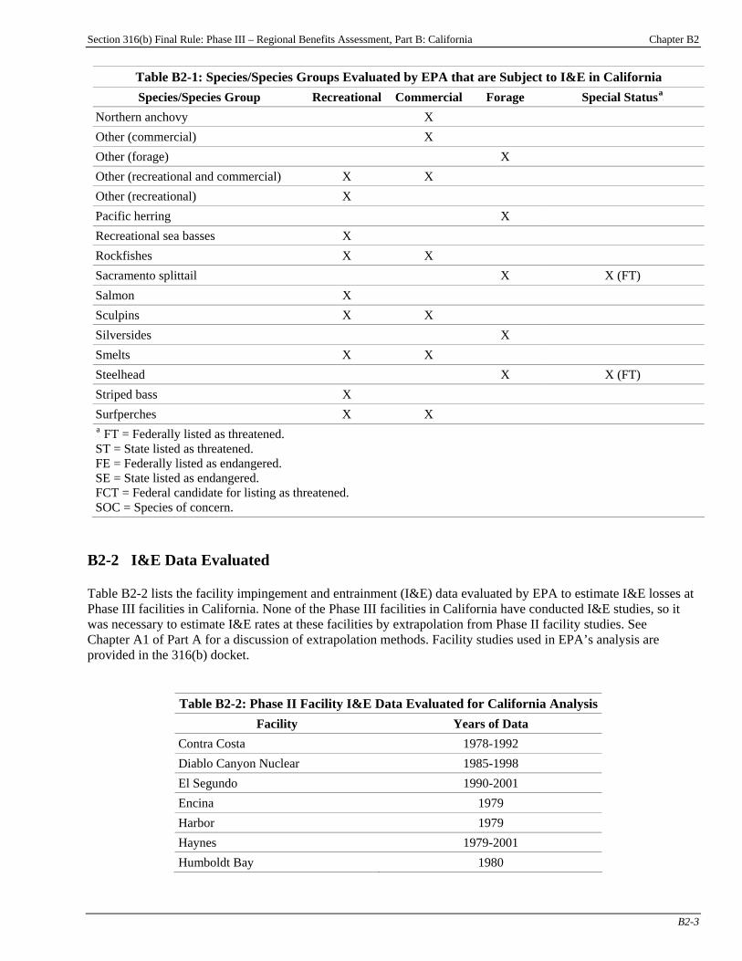
Section 316(b) Final Rule: Phase III – Regional Benefits Assessment, Part B: California Chapter B2
B2-3
Table B2-1: Species/Species Groups Evaluated by EPA that are Subject to I&E in California Species/Species Group Recreational Commercial Forage Special StatusP
aP
Northern anchovy X Other (commercial) X Other (forage) X Other (recreational and commercial) X X Other (recreational) X Pacific herring X Recreational sea basses X Rockfishes X X Sacramento splittail X X (FT) Salmon X Sculpins X X Silversides X Smelts X X Steelhead X X (FT) Striped bass X Surfperches X X P
aP FT = Federally listed as threatened.
ST = State listed as threatened. FE = Federally listed as endangered. SE = State listed as endangered. FCT = Federal candidate for listing as threatened. SOC = Species of concern.
B2-2 I&E Data Evaluated Table B2-2 lists the facility impingement and entrainment (I&E) data evaluated by EPA to estimate I&E losses at Phase III facilities in California. None of the Phase III facilities in California have conducted I&E studies, so it was necessary to estimate I&E rates at these facilities by extrapolation from Phase II facility studies. See Chapter A1 of Part A for a discussion of extrapolation methods. Facility studies used in EPA’s analysis are provided in the 316(b) docket.
Table B2-2: Phase II Facility I&E Data Evaluated for California AnalysisFacility Years of Data
Contra Costa 1978-1992 Diablo Canyon Nuclear 1985-1998 El Segundo 1990-2001 Encina 1979 Harbor 1979 Haynes 1979-2001 Humboldt Bay 1980
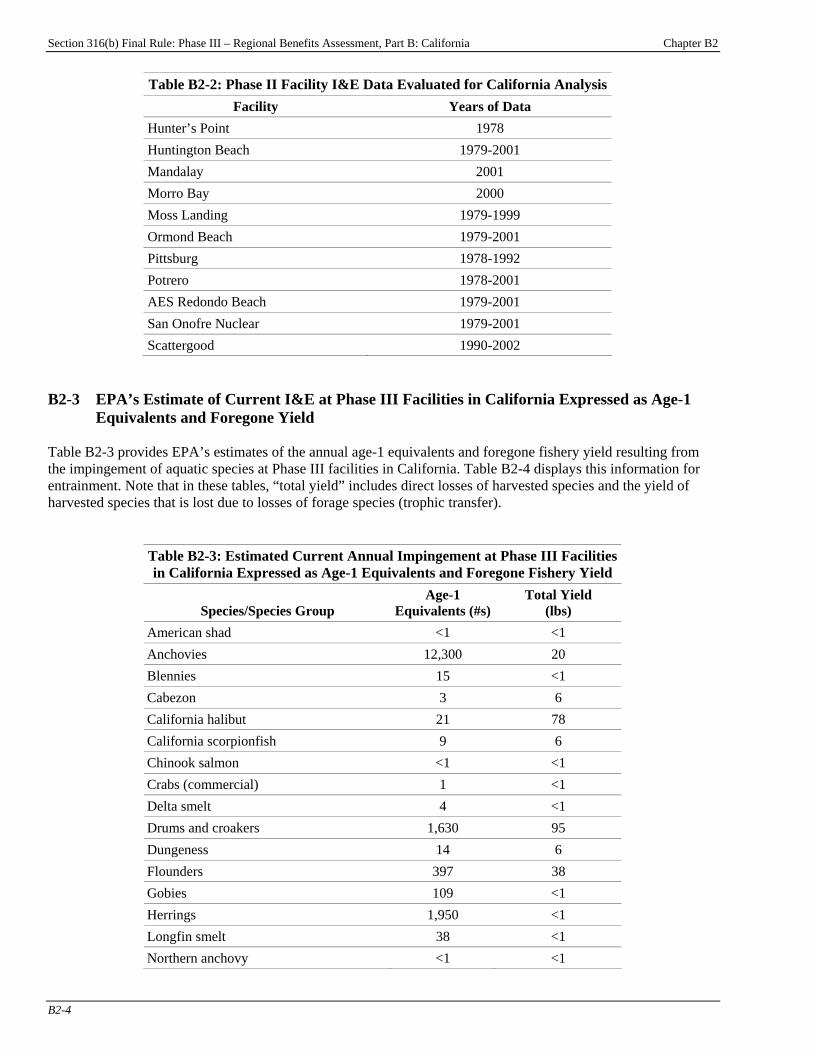
Section 316(b) Final Rule: Phase III – Regional Benefits Assessment, Part B: California Chapter B2
B2-4
Table B2-2: Phase II Facility I&E Data Evaluated for California Analysis Facility Years of Data
Hunter’s Point 1978 Huntington Beach 1979-2001 Mandalay 2001 Morro Bay 2000 Moss Landing 1979-1999 Ormond Beach 1979-2001 Pittsburg 1978-1992 Potrero 1978-2001 AES Redondo Beach 1979-2001 San Onofre Nuclear 1979-2001 Scattergood 1990-2002
B2-3 EPA’s Estimate of Current I&E at Phase III Facilities in California Expressed as Age-1
Equivalents and Foregone Yield Table B2-3 provides EPA’s estimates of the annual age-1 equivalents and foregone fishery yield resulting from the impingement of aquatic species at Phase III facilities in California. Table B2-4 displays this information for entrainment. Note that in these tables, “total yield” includes direct losses of harvested species and the yield of harvested species that is lost due to losses of forage species (trophic transfer).
Table B2-3: Estimated Current Annual Impingement at Phase III Facilities in California Expressed as Age-1 Equivalents and Foregone Fishery Yield
Species/Species Group Age-1
Equivalents (#s)Total Yield
(lbs) American shad <1 <1 Anchovies 12,300 20 Blennies 15 <1 Cabezon 3 6 California halibut 21 78 California scorpionfish 9 6 Chinook salmon <1 <1 Crabs (commercial) 1 <1 Delta smelt 4 <1 Drums and croakers 1,630 95 Dungeness 14 6 Flounders 397 38 Gobies 109 <1 Herrings 1,950 <1 Longfin smelt 38 <1 Northern anchovy <1 <1

Section 316(b) Final Rule: Phase III – Regional Benefits Assessment, Part B: California Chapter B2
B2-5
Table B2-3: Estimated Current Annual Impingement at Phase III Facilities in California Expressed as Age-1 Equivalents and Foregone Fishery Yield
Species/Species Group Age-1
Equivalents (#s)Total Yield
(lbs) Other (commercial) 4 1 Other (forage) 1,740 <1 Other (recreational and commercial) 34 7 Other (recreational) 75 15 Pacific herring <1 <1 Rockfishes 576 139 Sacramento splittail 5 <1 Salmon <1 <1 Sculpins 527 21 Sea basses (commercial) <1 <1 Sea basses (recreational) 37 9 Shrimp (commercial) 278 <1 Shrimp (forage) 10 <1 Silversides 3,290 <1 Smelts 212 5 Steelhead <1 <1 Striped bass 247 215 Surfperches 4,100 267 Trophic transferP
aP <1 32
P
aP Contribution of forage fish to yield based on trophic transfer (see Chapter A1).
Table B2-4: Estimated Current Annual Entrainment at Phase III Facilities in California Expressed as Age-1 Equivalents and Foregone Fishery Yield
Species/Species Group
Age-1 Equivalents
(#s) Total Yield
(lbs) American shad <1 <1 Anchovies 1,480 2 Blennies 467,000 <1 Cabezon 3,470 5,890 California halibut 4,040 15,200 California scorpionfish <1 <1 Chinook salmon <1 <1 Crabs (commercial) 127,000 26 Delta smelt 1 <1 Drums and croakers 18,600 1,090 Dungeness 446 206 Flounders 864 83

Section 316(b) Final Rule: Phase III – Regional Benefits Assessment, Part B: California Chapter B2
B2-6
Table B2-4: Estimated Current Annual Entrainment at Phase III Facilities in California Expressed as Age-1 Equivalents and Foregone Fishery Yield
Species/Species Group
Age-1 Equivalents
(#s) Total Yield
(lbs) Gobies 97,900 <1 Herrings 16,400 <1 Longfin smelt <1 <1 Northern anchovy <1 <1 Other (commercial) 306 60 Other (forage) 369,000 <1 Other (recreational and commercial) <1 <1 Other (recreational) 42 8 Pacific herring 200 <1 Rockfishes 372,000 89,700 Sacramento splittail <1 <1 Salmon <1 <1 Sculpins 25,300 1,000 Sea basses (commercial) <1 <1 Sea basses (recreational) 26,400 6,500 Shrimp (commercial) 36,800 1 Shrimp (forage) 116,000 <1 Silversides 108 <1 Smelts 12 <1 Steelhead <1 <1 Striped bass 62 54 Surfperches <1 <1 Trophic transferP
aP <1 244
P
aP Contribution of forage fish to yield based on trophic transfer (see Chapter A1).
B2-4 Reductions in I&E at Phase III Facilities in the California Region Under
Alternative Options Table B2-5 presents estimated reductions in I&E under the “50 MGD for All Waterbodies” option, the “200 MGD for All Waterbodies” option, and the “100 MGD for Certain Waterbodies” option. Reductions under all other options are presented in Appendix B2.
Table B2-5: Estimated Reductions in I&E Under Three Alternative Options
Option Age-One Equivalents
(#s) Foregone Fishery Yield
(lbs) 50 MGD All Option 474,000 33,400 200 MGD All Option 0 0 100 MGD Option 0 0
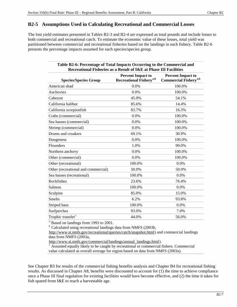
Section 316(b) Final Rule: Phase III – Regional Benefits Assessment, Part B: California Chapter B2
B2-7
B2-5 Assumptions Used in Calculating Recreational and Commercial Losses The lost yield estimates presented in Tables B2-3 and B2-4 are expressed as total pounds and include losses to both commercial and recreational catch. To estimate the economic value of these losses, total yield was partitioned between commercial and recreational fisheries based on the landings in each fishery. Table B2-6 presents the percentage impacts assumed for each species/species group.
Table B2-6: Percentage of Total Impacts Occurring to the Commercial and Recreational Fisheries as a Result of I&E at Phase III Facilities
Species/Species Group Percent Impact to
Recreational FisheryP
a,bP
Percent Impact to Commercial FisheryP
a,bP
American shad 0.0% 100.0% Anchovies 0.0% 100.0% Cabezon 45.9% 54.1% California halibut 85.6% 14.4% California scorpionfish 83.7% 16.3% Crabs (commercial) 0.0% 100.0% Sea basses (commercial) 0.0% 100.0% Shrimp (commercial) 0.0% 100.0% Drums and croakers 69.1% 30.9% Dungeness 0.0% 100.0% Flounders 1.0% 99.0% Northern anchovy 0.0% 100.0% Other (commercial) 0.0% 100.0% Other (recreational) 100.0% 0.0% Other (recreational and commercial) 50.0% 50.0% Sea basses (recreational) 100.0% 0.0% Rockfishes 23.6% 76.4% Salmon 100.0% 0.0% Sculpins 85.0% 15.0% Smelts 6.2% 93.8% Striped bass 100.0% 0.0% Surfperches 93.0% 7.0% Trophic transferP
cP 44.0% 56.0%
P
aP Based on landings from 1993 to 2001.
P
bP Calculated using recreational landings data from NMFS (2003b,
Uhttp://www.st.nmfs.gov/recreational/queries/catch/snapshot.htmlU) and commercial landings data from NMFS (2003a, Uhttp://www.st.nmfs.gov/commercial/landings/annual_landings.htmlU). P
cP Assumed equally likely to be caught by recreational or commercial fishers. Commercial
value calculated as overall average for region based on data from NMFS (2003a). See Chapter B3 for results of the commercial fishing benefits analysis and Chapter B4 for recreational fishing results. As discussed in Chapter A8, benefits were discounted to account for (1) the time to achieve compliance once a Phase III final regulation for existing facilities would have become effective, and (2) the time it takes for fish spared from I&E to reach a harvestable age.
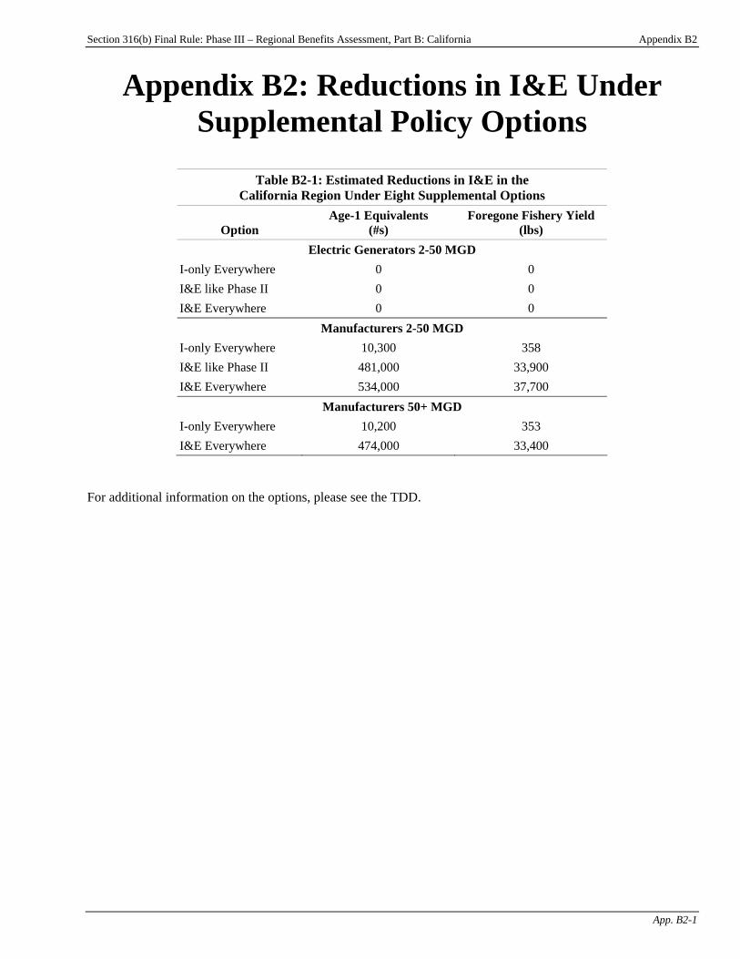
Section 316(b) Final Rule: Phase III – Regional Benefits Assessment, Part B: California Appendix B2
App. B2-1
Appendix B2: Reductions in I&E Under Supplemental Policy Options
Table B2-1: Estimated Reductions in I&E in the California Region Under Eight Supplemental Options
Option Age-1 Equivalents
(#s) Foregone Fishery Yield
(lbs) Electric Generators 2-50 MGD
I-only Everywhere 0 0 I&E like Phase II 0 0 I&E Everywhere 0 0
Manufacturers 2-50 MGD I-only Everywhere 10,300 358 I&E like Phase II 481,000 33,900 I&E Everywhere 534,000 37,700
Manufacturers 50+ MGD I-only Everywhere 10,200 353 I&E Everywhere 474,000 33,400
For additional information on the options, please see the TDD.
Section 316(b) Final Rule: Phase III – Regional Benefits Assessment, Part B: California Chapter B3
B3-1
Chapter B3: Commercial Fishing Benefits Introduction
Chapter Contents B3-1 Baseline Commercial Losses........................ B3-1 B3-2 Expected Benefits Under Regulatory
Analysis Options .......................................... B3-3 B3-2.1 Commercial Fishing Benefits of the “50 MGD for All Waterbodies”
Option ............................................. B3-3 B3-2.2 Commercial Fishing Benefits of the “200 MGD for All Waterbodies”
Option ............................................. B3-4 B3-2.3 Commercial Fishing Benefits of the “100 MGD for Certain Waterbodies” Option ...................... B3-4
This chapter presents the results of the commercial fishing benefits analysis for the California region. The chapter presents EPA’s estimates of baseline (i.e., current) annual commercial fishery losses from impingement and entrainment (I&E) at potentially regulated facilities in the California region and annual reductions in these losses under the regulatory analysis options for Phase III existing facilitiesPF
1FP:
< the “50 MGD for All Waterbodies” option, < the “200 MGD for All Waterbodies” option,
and < the “100 MGD for Certain Waterbodies”
option. The chapter then presents the estimated benefits to commercial fisheries from eliminating baseline losses from I&E, and the expected benefits under the regulatory analysis options. Results for the California region include commercial benefits from both Northern and Southern California. Chapter A4, “Methods for Estimating Commercial Fishing Benefits,” details the methods used by EPA to estimate the commercial fishing benefits of reducing and eliminating I&E losses. EPA considered a wide range of policy options in developing this regulation. In addition to the regulatory analysis options, EPA evaluated 8 supplemental options. Appendix B3 presents results of the commercial fishing benefits analysis for the supplemental options. B3-1 Baseline Commercial Losses Table B3-1 provides EPA’s estimate of the value of gross revenues lost in commercial fisheries resulting from the impingement of aquatic species at facilities in the California region. Table B3-2 displays this information for entrainment. Total annualized revenue losses are approximately $57,679 (undiscounted).
P
1P See the Introduction to this report for a description of the regulatory analysis options.
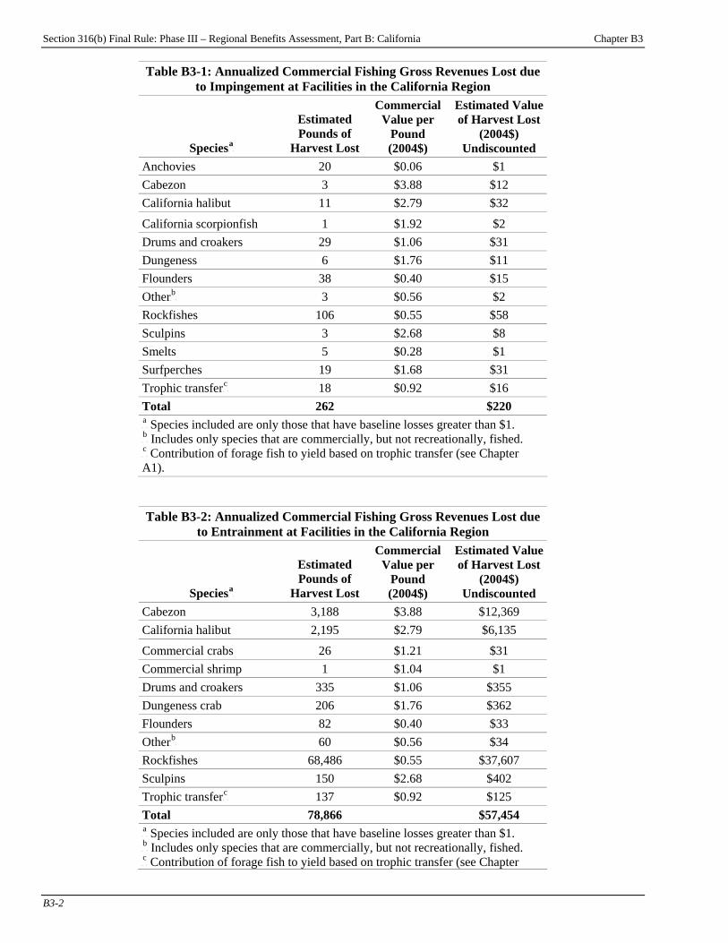
Section 316(b) Final Rule: Phase III – Regional Benefits Assessment, Part B: California Chapter B3
B3-2
Table B3-1: Annualized Commercial Fishing Gross Revenues Lost due to Impingement at Facilities in the California Region
SpeciesP
aP
Estimated Pounds of
Harvest Lost
Commercial Value per
Pound (2004$)
Estimated Value of Harvest Lost
(2004$) Undiscounted
Anchovies 20 $0.06 $1 Cabezon 3 $3.88 $12 California halibut 11 $2.79 $32
California scorpionfish 1 $1.92 $2 Drums and croakers 29 $1.06 $31 Dungeness 6 $1.76 $11 Flounders 38 $0.40 $15 OtherP
bP 3 $0.56 $2
Rockfishes 106 $0.55 $58 Sculpins 3 $2.68 $8 Smelts 5 $0.28 $1 Surfperches 19 $1.68 $31 Trophic transferP
cP 18 $0.92 $16
Total 262 $220 P
aP Species included are only those that have baseline losses greater than $1.
P
bP Includes only species that are commercially, but not recreationally, fished.
P
cP Contribution of forage fish to yield based on trophic transfer (see Chapter
A1).
Table B3-2: Annualized Commercial Fishing Gross Revenues Lost due to Entrainment at Facilities in the California Region
SpeciesP
aP
Estimated Pounds of
Harvest Lost
Commercial Value per
Pound (2004$)
Estimated Value of Harvest Lost
(2004$) Undiscounted
Cabezon 3,188 $3.88 $12,369 California halibut 2,195 $2.79 $6,135
Commercial crabs 26 $1.21 $31 Commercial shrimp 1 $1.04 $1 Drums and croakers 335 $1.06 $355 Dungeness crab 206 $1.76 $362 Flounders 82 $0.40 $33 OtherP
bP 60 $0.56 $34
Rockfishes 68,486 $0.55 $37,607 Sculpins 150 $2.68 $402 Trophic transferP
cP 137 $0.92 $125
Total 78,866 $57,454 P
aP Species included are only those that have baseline losses greater than $1.
P
bP Includes only species that are commercially, but not recreationally, fished.
P
cP Contribution of forage fish to yield based on trophic transfer (see Chapter
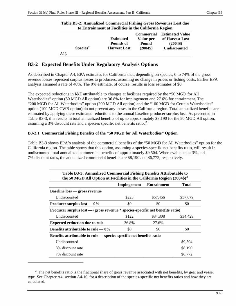
Section 316(b) Final Rule: Phase III – Regional Benefits Assessment, Part B: California Chapter B3
B3-3
Table B3-2: Annualized Commercial Fishing Gross Revenues Lost due to Entrainment at Facilities in the California Region
SpeciesP
aP
Estimated Pounds of
Harvest Lost
Commercial Value per
Pound (2004$)
Estimated Value of Harvest Lost
(2004$) Undiscounted
A1). B3-2 Expected Benefits Under Regulatory Analysis Options As described in Chapter A4, EPA estimates for California that, depending on species, 0 to 74% of the gross revenue losses represent surplus losses to producers, assuming no change in prices or fishing costs. Earlier EPA analysis assumed a rate of 40%. The 0% estimate, of course, results in loss estimates of $0. The expected reductions in I&E attributable to changes at facilities required by the “50 MGD for All Waterbodies” option (50 MGD All option) are 36.8% for impingement and 27.6% for entrainment. The “200 MGD for All Waterbodies” option (200 MGD All option) and the “100 MGD for Certain Waterbodies” option (100 MGD CWB option) do not prevent any losses in the California region. Total annualized benefits are estimated by applying these estimated reductions to the annual baseline producer surplus loss. As presented in Table B3-3, this results in total annualized benefits of up to approximately $8,190 for the 50 MGD All option, assuming a 3% discount rate and a species specific net benefits ratio.TPF
2FPT
B3-2.1 Commercial Fishing Benefits of the “50 MGD for All Waterbodies” Option Table B3-3 shows EPA’s analysis of the commercial benefits of the “50 MGD for All Waterbodies” option for the California region. The table shows that this option, assuming a species-specific net benefits ratio, will result in undiscounted total annualized commercial benefits of approximately $9,504. When evaluated at 3% and 7% discount rates, the annualized commercial benefits are $8,190 and $6,772, respectively.
Table B3-3: Annualized Commercial Fishing Benefits Attributable to the 50 MGD All Option at Facilities in the California Region (2004$)P
aP
Impingement Entrainment Total Baseline loss — gross revenue
Undiscounted $223 $57,456 $57,679 Producer surplus lost — 0% $0 $0 $0 Producer surplus lost — (gross revenue * species-specific net benefits ratio)
Undiscounted $122 $34,308 $34,429 Expected reduction due to rule 36.8% 27.6% Benefits attributable to rule — 0% $0 $0 $0 Benefits attributable to rule — species-specific net benefits ratio
Undiscounted $9,504 3% discount rate $8,190 7% discount rate $6,772
TP
2PT The net benefits ratio is the fractional share of gross revenue associated with net benefits, by gear and vessel
type. See Chapter A4, section A4-10, for a description of the species-specific net benefits ratios and how they are calculated.
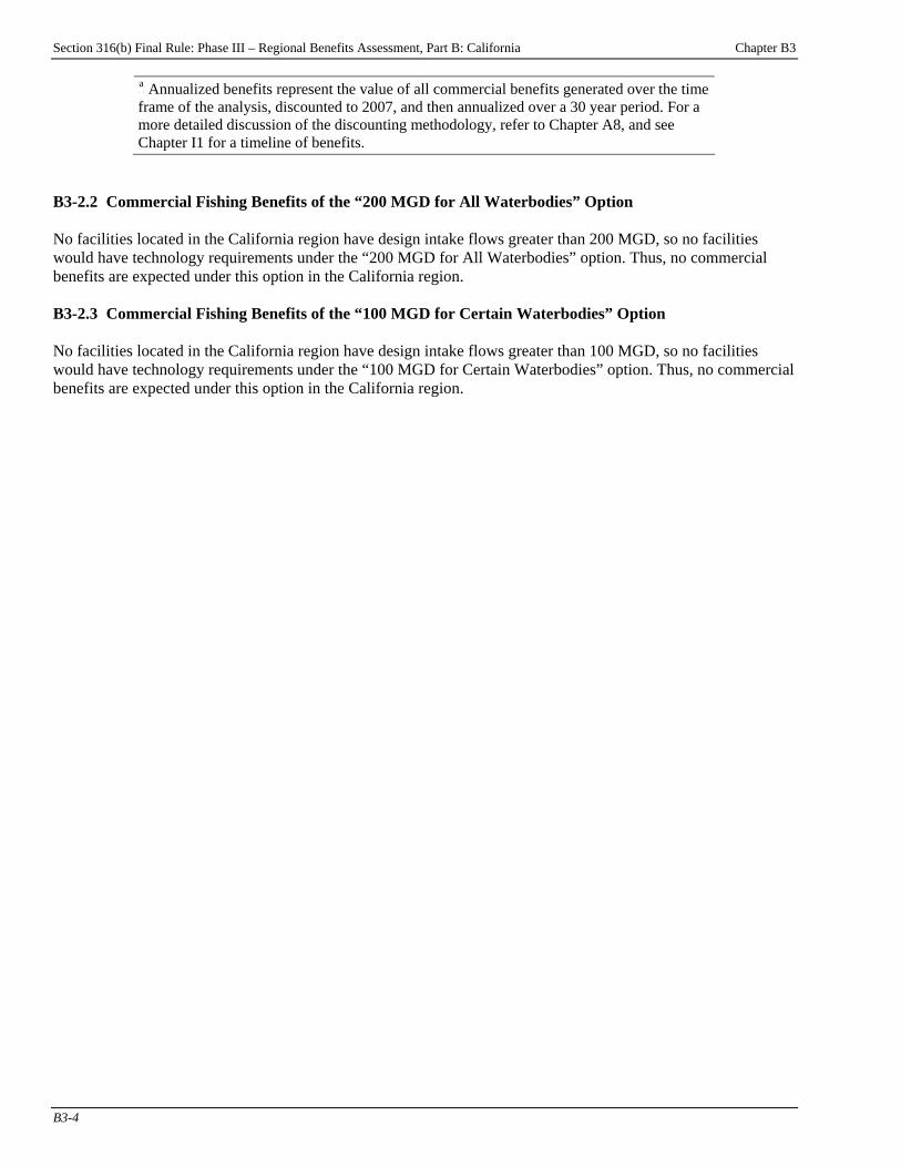
Section 316(b) Final Rule: Phase III – Regional Benefits Assessment, Part B: California Chapter B3
B3-4
P
aP Annualized benefits represent the value of all commercial benefits generated over the time
frame of the analysis, discounted to 2007, and then annualized over a 30 year period. For a more detailed discussion of the discounting methodology, refer to Chapter A8, and see Chapter I1 for a timeline of benefits.
B3-2.2 Commercial Fishing Benefits of the “200 MGD for All Waterbodies” Option No facilities located in the California region have design intake flows greater than 200 MGD, so no facilities would have technology requirements under the “200 MGD for All Waterbodies” option. Thus, no commercial benefits are expected under this option in the California region. B3-2.3 Commercial Fishing Benefits of the “100 MGD for Certain Waterbodies” Option No facilities located in the California region have design intake flows greater than 100 MGD, so no facilities would have technology requirements under the “100 MGD for Certain Waterbodies” option. Thus, no commercial benefits are expected under this option in the California region.
Section 316(b) Final Rule: Phase III – Regional Benefits Assessment, Part B: California Appendix B3
App. B3-1
Appendix B3: Commercial Fishing Benefits Under Supplemental Policy Options
Introduction Chapter B3 presents EPA’s estimates of the commercial benefits of the regulatory options for the section 316(b) rule for Phase III facilities in the California region. To facilitate comparisons among the options, this appendix presents estimates of the commercial fishing benefits of several supplemental options that EPA evaluated in preparation for this rule:
Appendix Contents B3-1 Commercial Fishing Benefits of the Supplemental Options ................................ B3-1
< “Electric Generators 2-50 MGD I-only Everywhere” option; < “Electric Generators 2-50 MGD I&E like Phase II” option; < “Electric Generators 2-50 MGD I&E Everywhere” option; < “Manufacturers 2-50 MGD I-only Everywhere” option; < “Manufacturers 2-50 MGD I&E like Phase II” option; < “Manufacturers 2-50 MGD I&E Everywhere” option; < “Manufacturers 50+ MGD I-only Everywhere” option; and < “Manufacturers 50+ MGD I&E Everywhere” option.
Commercial fishing benefits presented in this chapter were estimated using the benefit transfer approach discussed in Chapter B3 and in Chapter A4, “Methods for Estimating Commercial Fishing Benefits.” B3-1 Commercial Fishing Benefits of the Supplemental Options No facilities located in the California region are electric generators with design intake flows greater than 2 MGD and less than 50 MGD, so no facilities would have technology requirements under the “Electric Generators 2-50 MGD I-only Everywhere” option, the “Electric Generators 2-50 MGD I&E like Phase II” option, or the “Electric Generators 2-50 MGD I&E Everywhere” option. Thus no commercial benefits are expected under these options in the California region. For additional information on the options, please see the TDD. Tables B3-1 through B3-5 present EPA’s estimates of the annualized commercial benefits of the remaining supplemental options in the California region.

Section 316(b) Final Rule: Phase III – Regional Benefits Assessment, Part B: California Appendix B3
App. B3-2
Table B3-1: Annualized Commercial Fishing Benefits Attributable to the “Manufacturers 2-50 MGD I-only Everywhere” Option at Facilities in the
California Region (2004$)P
aP
Impingement Entrainment Total Baseline loss — gross revenue
Undiscounted $223 $57,456 $57,679 Producer surplus lost — 0% $0 $0 $0 Producer surplus lost — (gross revenue * species-specific net benefits ratio)
Undiscounted $122 $34,308 $34,429 Expected reduction due to rule 37% 0% Benefits attributable to rule — 0% $0 $0 $0 Benefits attributable to rule — species-specific net benefits ratio
Undiscounted $45 3% discount rate $36 7% discount rate $26
P
aP Annualized benefits represent the value of all commercial benefits generated over the time
frame of the analysis, discounted to 2007, and then annualized over a thirty year period. For a more detailed discussion of the discounting methodology, refer to Chapter A8, and see Chapter I1 for a timeline of benefits.
Table B3-2: Annualized Commercial Fishing Benefits Attributable to the “Manufacturers 2-50 MGD I&E like Phase II” Option at Facilities in the
California Region (2004$)P
aP
Impingement Entrainment Total Baseline loss — gross revenue
Undiscounted $223 $57,456 $57,679 Producer surplus lost — 0% $0 $0 $0 Producer surplus lost — (gross revenue * species-specific net benefits ratio)
Undiscounted $122 $34,308 $34,429 Expected reduction due to rule 37% 28% Benefits attributable to rule — 0% $0 $0 $0 Benefits attributable to rule — species-specific net benefits ratio
Undiscounted $9,638 3% discount rate $7,602 7% discount rate $5,606
P
aP Annualized benefits represent the value of all commercial benefits generated over the time
frame of the analysis, discounted to 2007, and then annualized over a thirty year period. For a more detailed discussion of the discounting methodology, refer to Chapter A8, and see Chapter I1 for a timeline of benefits.
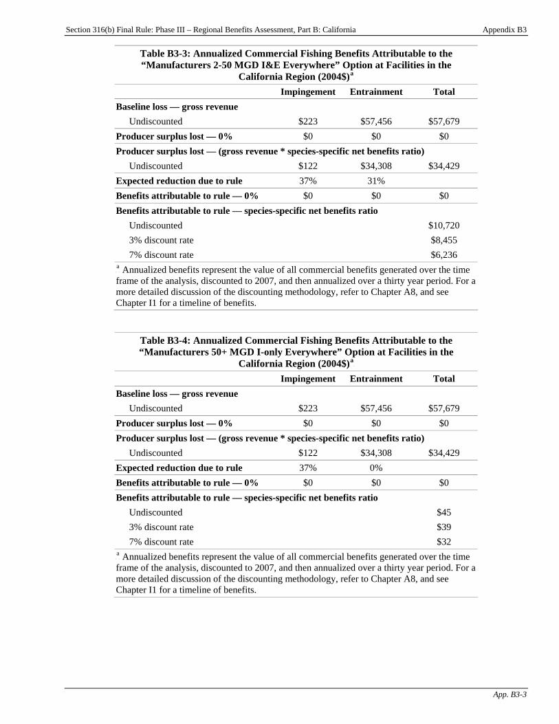
Section 316(b) Final Rule: Phase III – Regional Benefits Assessment, Part B: California Appendix B3
App. B3-3
Table B3-3: Annualized Commercial Fishing Benefits Attributable to the “Manufacturers 2-50 MGD I&E Everywhere” Option at Facilities in the
California Region (2004$)P
aP
Impingement Entrainment Total Baseline loss — gross revenue
Undiscounted $223 $57,456 $57,679 Producer surplus lost — 0% $0 $0 $0 Producer surplus lost — (gross revenue * species-specific net benefits ratio)
Undiscounted $122 $34,308 $34,429 Expected reduction due to rule 37% 31% Benefits attributable to rule — 0% $0 $0 $0 Benefits attributable to rule — species-specific net benefits ratio
Undiscounted $10,720 3% discount rate $8,455 7% discount rate $6,236
P
aP Annualized benefits represent the value of all commercial benefits generated over the time
frame of the analysis, discounted to 2007, and then annualized over a thirty year period. For a more detailed discussion of the discounting methodology, refer to Chapter A8, and see Chapter I1 for a timeline of benefits.
Table B3-4: Annualized Commercial Fishing Benefits Attributable to the “Manufacturers 50+ MGD I-only Everywhere” Option at Facilities in the
California Region (2004$)P
aP
Impingement Entrainment Total Baseline loss — gross revenue
Undiscounted $223 $57,456 $57,679 Producer surplus lost — 0% $0 $0 $0 Producer surplus lost — (gross revenue * species-specific net benefits ratio)
Undiscounted $122 $34,308 $34,429 Expected reduction due to rule 37% 0% Benefits attributable to rule — 0% $0 $0 $0 Benefits attributable to rule — species-specific net benefits ratio
Undiscounted $45 3% discount rate $39 7% discount rate $32
P
aP Annualized benefits represent the value of all commercial benefits generated over the time
frame of the analysis, discounted to 2007, and then annualized over a thirty year period. For a more detailed discussion of the discounting methodology, refer to Chapter A8, and see Chapter I1 for a timeline of benefits.
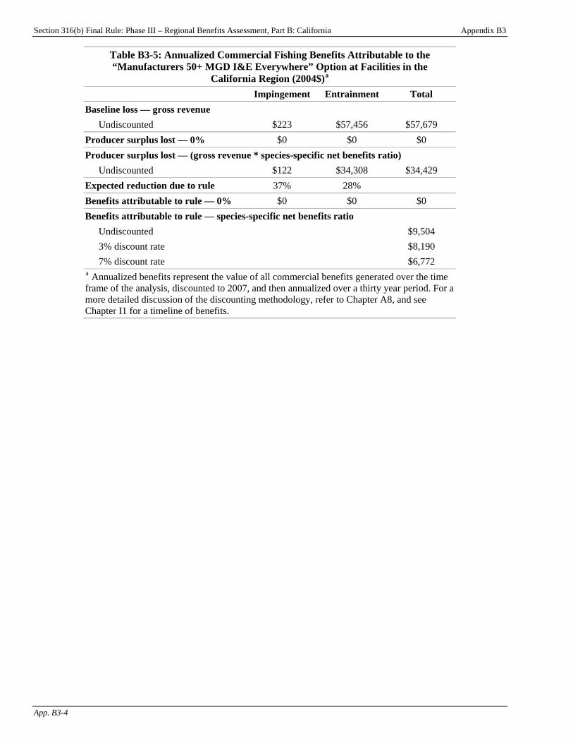
Section 316(b) Final Rule: Phase III – Regional Benefits Assessment, Part B: California Appendix B3
App. B3-4
Table B3-5: Annualized Commercial Fishing Benefits Attributable to the “Manufacturers 50+ MGD I&E Everywhere” Option at Facilities in the
California Region (2004$)P
aP
Impingement Entrainment Total Baseline loss — gross revenue
Undiscounted $223 $57,456 $57,679 Producer surplus lost — 0% $0 $0 $0 Producer surplus lost — (gross revenue * species-specific net benefits ratio)
Undiscounted $122 $34,308 $34,429 Expected reduction due to rule 37% 28% Benefits attributable to rule — 0% $0 $0 $0 Benefits attributable to rule — species-specific net benefits ratio
Undiscounted $9,504 3% discount rate $8,190 7% discount rate $6,772
P
aP Annualized benefits represent the value of all commercial benefits generated over the time
frame of the analysis, discounted to 2007, and then annualized over a thirty year period. For a more detailed discussion of the discounting methodology, refer to Chapter A8, and see Chapter I1 for a timeline of benefits.
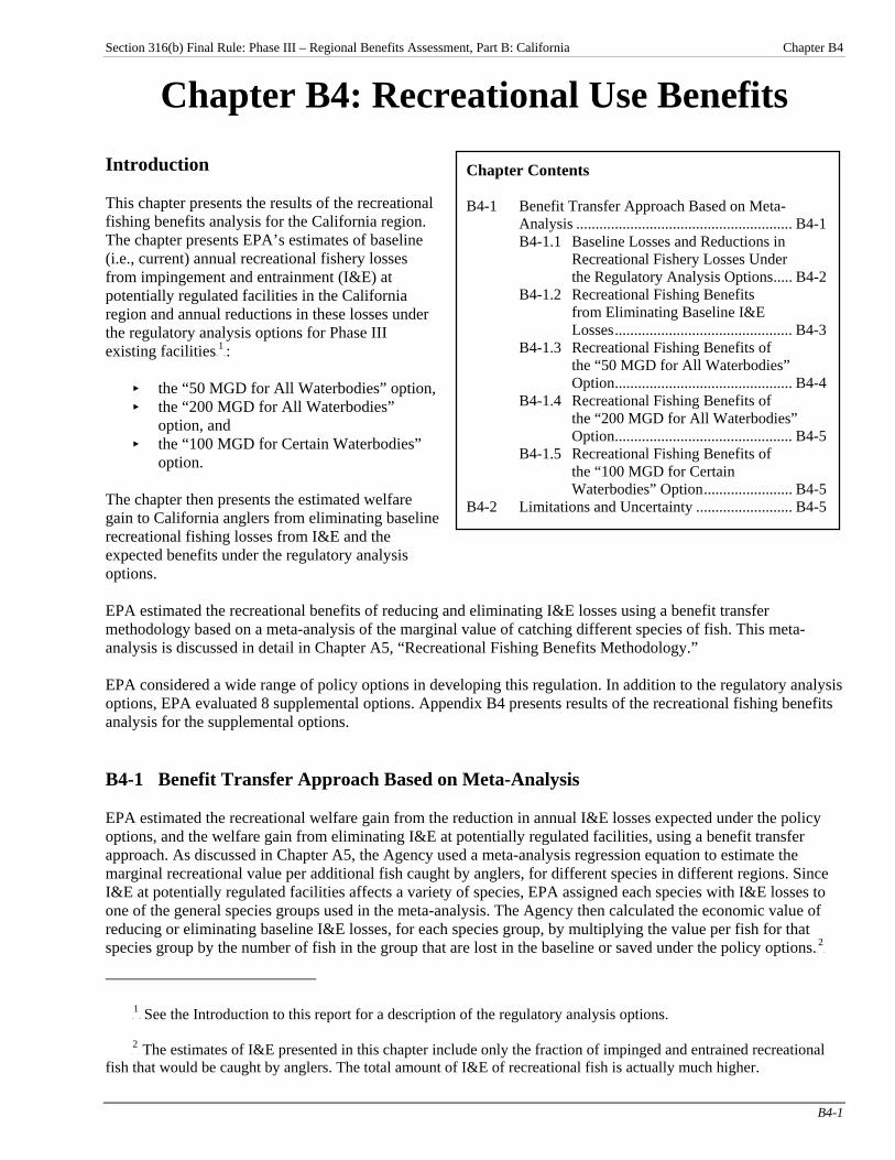
Section 316(b) Final Rule: Phase III – Regional Benefits Assessment, Part B: California Chapter B4
B4-1
Chapter B4: Recreational Use Benefits
Chapter Contents B4-1 Benefit Transfer Approach Based on Meta- Analysis ........................................................ B4-1 B4-1.1 Baseline Losses and Reductions in Recreational Fishery Losses Under the Regulatory Analysis Options..... B4-2 B4-1.2 Recreational Fishing Benefits from Eliminating Baseline I&E Losses.............................................. B4-3 B4-1.3 Recreational Fishing Benefits of the “50 MGD for All Waterbodies” Option.............................................. B4-4 B4-1.4 Recreational Fishing Benefits of the “200 MGD for All Waterbodies” Option.............................................. B4-5 B4-1.5 Recreational Fishing Benefits of the “100 MGD for Certain Waterbodies” Option....................... B4-5 B4-2 Limitations and Uncertainty ......................... B4-5
Introduction This chapter presents the results of the recreational fishing benefits analysis for the California region. The chapter presents EPA’s estimates of baseline (i.e., current) annual recreational fishery losses from impingement and entrainment (I&E) at potentially regulated facilities in the California region and annual reductions in these losses under the regulatory analysis options for Phase III existing facilitiesTPF
1FPT:
< the “50 MGD for All Waterbodies” option, < the “200 MGD for All Waterbodies”
option, and < the “100 MGD for Certain Waterbodies”
option. The chapter then presents the estimated welfare gain to California anglers from eliminating baseline recreational fishing losses from I&E and the expected benefits under the regulatory analysis options. EPA estimated the recreational benefits of reducing and eliminating I&E losses using a benefit transfer methodology based on a meta-analysis of the marginal value of catching different species of fish. This meta-analysis is discussed in detail in Chapter A5, “Recreational Fishing Benefits Methodology.” EPA considered a wide range of policy options in developing this regulation. In addition to the regulatory analysis options, EPA evaluated 8 supplemental options. Appendix B4 presents results of the recreational fishing benefits analysis for the supplemental options. B4-1 Benefit Transfer Approach Based on Meta-Analysis EPA estimated the recreational welfare gain from the reduction in annual I&E losses expected under the policy options, and the welfare gain from eliminating I&E at potentially regulated facilities, using a benefit transfer approach. As discussed in Chapter A5, the Agency used a meta-analysis regression equation to estimate the marginal recreational value per additional fish caught by anglers, for different species in different regions. Since I&E at potentially regulated facilities affects a variety of species, EPA assigned each species with I&E losses to one of the general species groups used in the meta-analysis. The Agency then calculated the economic value of reducing or eliminating baseline I&E losses, for each species group, by multiplying the value per fish for that species group by the number of fish in the group that are lost in the baseline or saved under the policy options.PF
2FP
TP
1PT See the Introduction to this report for a description of the regulatory analysis options.
P
2P The estimates of I&E presented in this chapter include only the fraction of impinged and entrained recreational
fish that would be caught by anglers. The total amount of I&E of recreational fish is actually much higher.

Section 316(b) Final Rule: Phase III – Regional Benefits Assessment, Part B: California Chapter B4
B4-2
In general, the fit between the species with I&E losses and the species groups in the meta-analysis was good. However, EPA’s estimates of baseline I&E losses and reductions in I&E under the policy options included losses of “unidentified” species. The “unidentified” group includes fish lost indirectly through trophic transfer, as well as species for which no species information was available.PF
3FP Rather than using the meta-analysis regression to try to
predict the value per fish for an “unidentified” species, EPA assumed that per-fish values for these species can be approximated by the weighted average value per fish for all species affected by I&E in the California region.PF
4FP
B4-1.1 Baseline Losses and Reductions in Recreational Fishery Losses Under the Regulatory Analysis
Options Table B4-1 presents EPA’s estimates of baseline (i.e., current) annual recreational I&E losses at potentially regulated facilities, and annual reductions in these losses under each of the regulatory analysis options, in the California region. The table shows that total baseline losses to recreational fisheries are 32.8 thousand fish per year. In comparison, the “50 MGD for All Waterbodies” option prevents losses of 9.2 thousand fish per year. The “200 MGD for All Waterbodies” option and the “100 MGD for Certain Waterbodies” option do not prevent any losses in the California region. Of all the affected species, rockfish and sculpin have the highest losses in the baseline and the highest prevented losses under the “50 MGD for All Waterbodies” option.
P
3P In addition to recreational fish that are lost because they are impinged or entrained, some recreational fish are lost
because the forage fish that they feed on are impinged or entrained, and thus removed from the food chain. These trophic transfer losses of recreational species are included in EPA’s estimates of total I&E losses. Since it is difficult to predict which recreational species would be affected by losses of forage fish, these losses are classified as “unidentified” recreational species. Also included in the “unidentified” group are losses of fish that were reported by facilities without information about their exact species.
P
4P EPA used the estimated level of baseline recreational losses for each species group as a weighting factor.
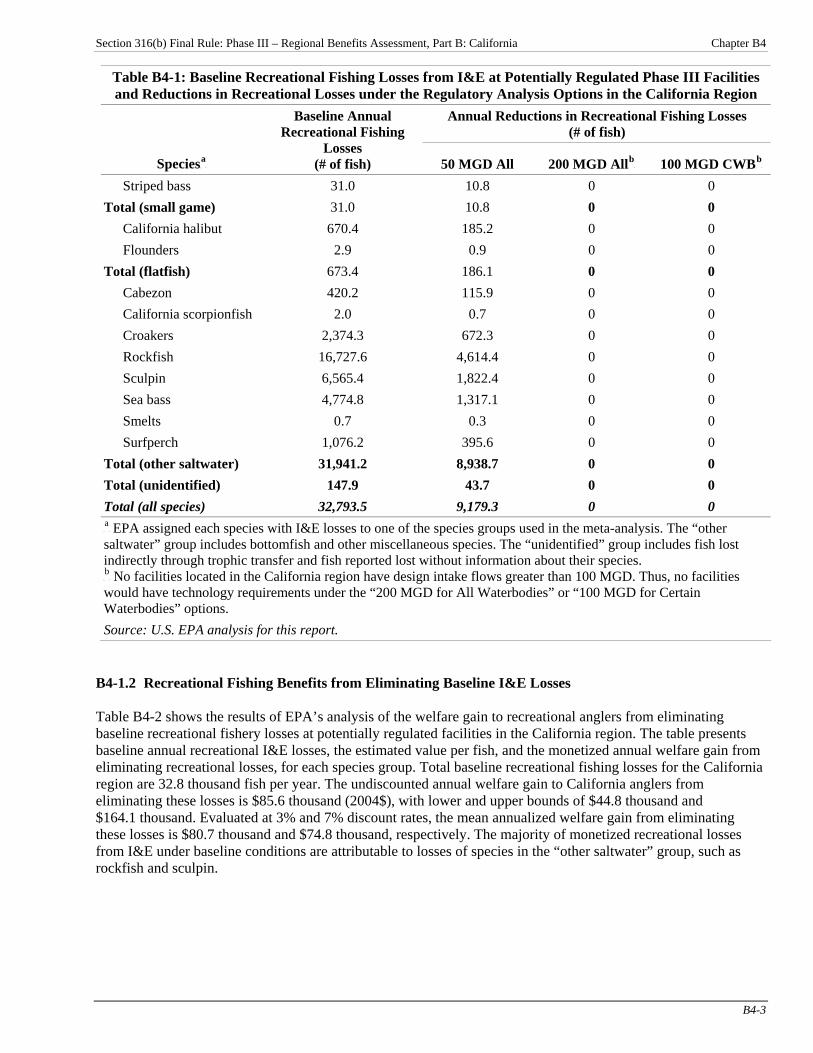
Section 316(b) Final Rule: Phase III – Regional Benefits Assessment, Part B: California Chapter B4
B4-3
Table B4-1: Baseline Recreational Fishing Losses from I&E at Potentially Regulated Phase III Facilities and Reductions in Recreational Losses under the Regulatory Analysis Options in the California Region
Annual Reductions in Recreational Fishing Losses (# of fish)
SpeciesP
aP
Baseline Annual Recreational Fishing
Losses (# of fish) 50 MGD All 200 MGD AllP
bP 100 MGD CWBP
bP
Striped bass 31.0 10.8 0 0 Total (small game) 31.0 10.8 0 0
California halibut 670.4 185.2 0 0 Flounders 2.9 0.9 0 0
Total (flatfish) 673.4 186.1 0 0 Cabezon 420.2 115.9 0 0 California scorpionfish 2.0 0.7 0 0 Croakers 2,374.3 672.3 0 0 Rockfish 16,727.6 4,614.4 0 0 Sculpin 6,565.4 1,822.4 0 0 Sea bass 4,774.8 1,317.1 0 0 Smelts 0.7 0.3 0 0 Surfperch 1,076.2 395.6 0 0
Total (other saltwater) 31,941.2 8,938.7 0 0 Total (unidentified) 147.9 43.7 0 0 Total (all species) 32,793.5 9,179.3 0 0 P
aP EPA assigned each species with I&E losses to one of the species groups used in the meta-analysis. The “other
saltwater” group includes bottomfish and other miscellaneous species. The “unidentified” group includes fish lost indirectly through trophic transfer and fish reported lost without information about their species. P
bP No facilities located in the California region have design intake flows greater than 100 MGD. Thus, no facilities
would have technology requirements under the “200 MGD for All Waterbodies” or “100 MGD for Certain Waterbodies” options. Source: U.S. EPA analysis for this report.
B4-1.2 Recreational Fishing Benefits from Eliminating Baseline I&E Losses Table B4-2 shows the results of EPA’s analysis of the welfare gain to recreational anglers from eliminating baseline recreational fishery losses at potentially regulated facilities in the California region. The table presents baseline annual recreational I&E losses, the estimated value per fish, and the monetized annual welfare gain from eliminating recreational losses, for each species group. Total baseline recreational fishing losses for the California region are 32.8 thousand fish per year. The undiscounted annual welfare gain to California anglers from eliminating these losses is $85.6 thousand (2004$), with lower and upper bounds of $44.8 thousand and $164.1 thousand. Evaluated at 3% and 7% discount rates, the mean annualized welfare gain from eliminating these losses is $80.7 thousand and $74.8 thousand, respectively. The majority of monetized recreational losses from I&E under baseline conditions are attributable to losses of species in the “other saltwater” group, such as rockfish and sculpin.
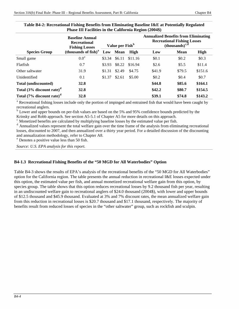
Section 316(b) Final Rule: Phase III – Regional Benefits Assessment, Part B: California Chapter B4
B4-4
Table B4-2: Recreational Fishing Benefits from Eliminating Baseline I&E at Potentially Regulated Phase III Facilities in the California Region (2004$)
Value per FishP
bP
Annualized Benefits from Eliminating Recreational Fishing Losses
(thousands)P
c,dP
Species Group
Baseline Annual Recreational
Fishing Losses (thousands of fish)P
aP Low Mean High Low Mean High
Small game 0.0P
eP $3.34 $6.11 $11.16 $0.1 $0.2 $0.3
Flatfish 0.7 $3.93 $8.22 $16.94 $2.6 $5.5 $11.4 Other saltwater 31.9 $1.31 $2.49 $4.75 $41.9 $79.5 $151.6 Unidentified 0.1 $1.37 $2.61 $5.00 $0.2 $0.4 $0.7 Total (undiscounted) 32.8 $44.8 $85.6 $164.1 Total (3% discount rate)P
dP 32.8 $42.2 $80.7 $154.5
Total (7% discount rate)P
dP 32.8 $39.1 $74.8 $143.2
P
aP Recreational fishing losses include only the portion of impinged and entrained fish that would have been caught by
recreational anglers. P
bP Lower and upper bounds on per-fish values are based on the 5% and 95% confidence bounds predicted by the
Krinsky and Robb approach. See section A5-5.1 of Chapter A5 for more details on this approach. P
cP Monetized benefits are calculated by multiplying baseline losses by the estimated value per fish.
P
dP Annualized values represent the total welfare gain over the time frame of the analysis from eliminating recreational
losses, discounted to 2007, and then annualized over a thirty year period. For a detailed discussion of the discounting and annualization methodology, refer to Chapter A8. P
eP Denotes a positive value less than 50 fish.
Source: U.S. EPA analysis for this report. B4-1.3 Recreational Fishing Benefits of the “50 MGD for All Waterbodies” Option Table B4-3 shows the results of EPA’s analysis of the recreational benefits of the “50 MGD for All Waterbodies” option for the California region. The table presents the annual reduction in recreational I&E losses expected under this option, the estimated value per fish, and annual monetized recreational welfare gain from this option, by species group. The table shows that this option reduces recreational losses by 9.2 thousand fish per year, resulting in an undiscounted welfare gain to recreational anglers of $24.0 thousand (2004$), with lower and upper bounds of $12.5 thousand and $45.9 thousand. Evaluated at 3% and 7% discount rates, the mean annualized welfare gain from this reduction in recreational losses is $20.7 thousand and $17.1 thousand, respectively. The majority of benefits result from reduced losses of species in the “other saltwater” group, such as rockfish and sculpin.
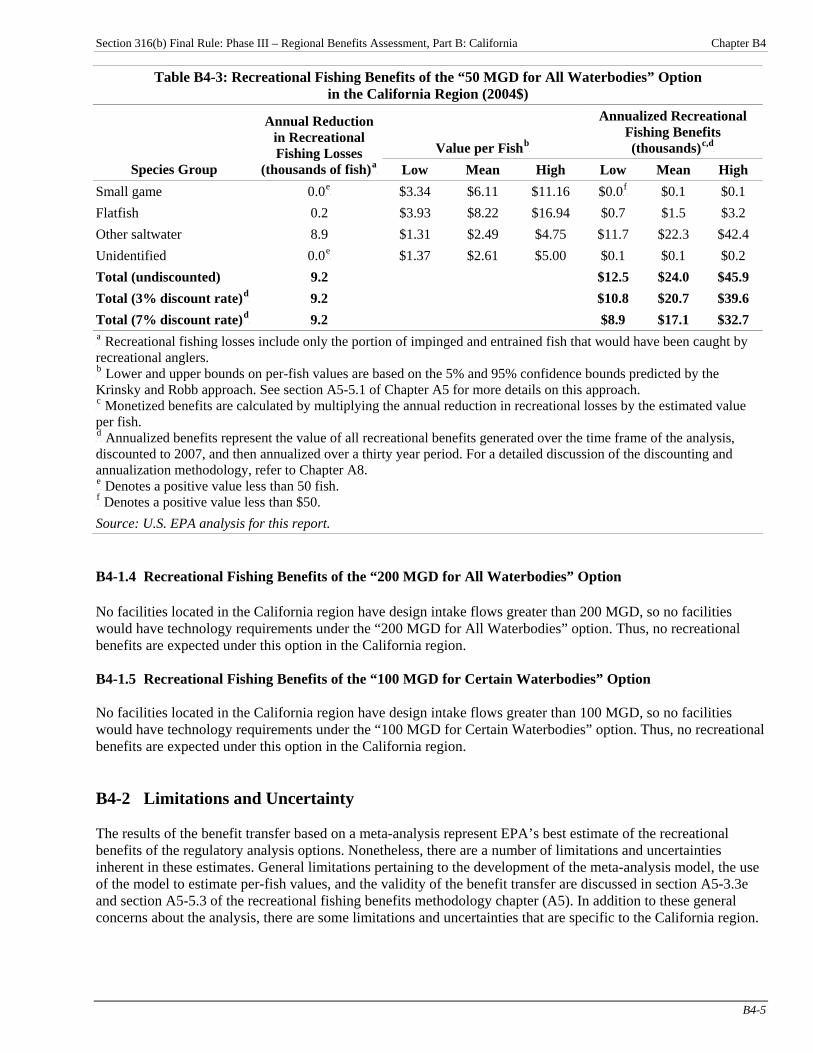
Section 316(b) Final Rule: Phase III – Regional Benefits Assessment, Part B: California Chapter B4
B4-5
Table B4-3: Recreational Fishing Benefits of the “50 MGD for All Waterbodies” Option in the California Region (2004$)
Value per FishP
bP
Annualized Recreational Fishing Benefits (thousands)P
c,dP
Species Group
Annual Reduction in Recreational Fishing Losses
(thousands of fish)P
aP Low Mean High Low Mean High
Small game 0.0P
eP $3.34 $6.11 $11.16 $0.0P
fP $0.1 $0.1
Flatfish 0.2 $3.93 $8.22 $16.94 $0.7 $1.5 $3.2 Other saltwater 8.9 $1.31 $2.49 $4.75 $11.7 $22.3 $42.4 Unidentified 0.0P
eP $1.37 $2.61 $5.00 $0.1 $0.1 $0.2
Total (undiscounted) 9.2 $12.5 $24.0 $45.9 Total (3% discount rate)P
dP 9.2 $10.8 $20.7 $39.6
Total (7% discount rate)P
dP 9.2 $8.9 $17.1 $32.7
P
aP Recreational fishing losses include only the portion of impinged and entrained fish that would have been caught by
recreational anglers. P
bP Lower and upper bounds on per-fish values are based on the 5% and 95% confidence bounds predicted by the
Krinsky and Robb approach. See section A5-5.1 of Chapter A5 for more details on this approach. P
cP Monetized benefits are calculated by multiplying the annual reduction in recreational losses by the estimated value
per fish. P
dP Annualized benefits represent the value of all recreational benefits generated over the time frame of the analysis,
discounted to 2007, and then annualized over a thirty year period. For a detailed discussion of the discounting and annualization methodology, refer to Chapter A8. P
eP Denotes a positive value less than 50 fish.
P
fP Denotes a positive value less than $50.
Source: U.S. EPA analysis for this report. B4-1.4 Recreational Fishing Benefits of the “200 MGD for All Waterbodies” Option No facilities located in the California region have design intake flows greater than 200 MGD, so no facilities would have technology requirements under the “200 MGD for All Waterbodies” option. Thus, no recreational benefits are expected under this option in the California region. B4-1.5 Recreational Fishing Benefits of the “100 MGD for Certain Waterbodies” Option No facilities located in the California region have design intake flows greater than 100 MGD, so no facilities would have technology requirements under the “100 MGD for Certain Waterbodies” option. Thus, no recreational benefits are expected under this option in the California region. B4-2 Limitations and Uncertainty The results of the benefit transfer based on a meta-analysis represent EPA’s best estimate of the recreational benefits of the regulatory analysis options. Nonetheless, there are a number of limitations and uncertainties inherent in these estimates. General limitations pertaining to the development of the meta-analysis model, the use of the model to estimate per-fish values, and the validity of the benefit transfer are discussed in section A5-3.3e and section A5-5.3 of the recreational fishing benefits methodology chapter (A5). In addition to these general concerns about the analysis, there are some limitations and uncertainties that are specific to the California region.

Section 316(b) Final Rule: Phase III – Regional Benefits Assessment, Part B: California Chapter B4
B4-6
The main limitation of applying the meta-analysis to the California region is that California is a large state with varied recreational fishing resources. The species that are targeted in the northern and southern parts of the state are somewhat different, and assigning a single value to each species based on an average for California may introduce some error into the resulting benefit estimates.
Section 316(b) Final Rule: Phase III – Regional Benefits Assessment, Part B: California Appendix B4
App. B4-1
Appendix B4: Recreational Use Benefits Under Supplemental Policy Options
Introduction
Appendix Contents B4-1 Recreational Fishing Benefits of the Supplemental Options ................................ B4-1 B4-1.1 Estimated Reductions in Recreational Fishing Losses Under the Supplemental Options ............ B4-1 B4-1.2 Recreational Fishing Benefits of the Supplemental Options ............ B4-3 B4-2 Comparison of Recreational Fishing Benefits by Option ..................................... B4-6
Chapter B4 presents EPA’s estimates of the recreational benefits of the regulatory options for the section 316(b) rule for Phase III facilities in the California region. To facilitate comparisons among the options, this appendix presents estimates of the recreational fishing benefits of supplemental options that EPA evaluated in preparation for this rule:
< “Electric Generators 2-50 MGD I-only Everywhere” option;
< “Electric Generators 2-50 MGD I&E like Phase II” option;
< “Electric Generators 2-50 MGD I&E Everywhere” option; < “Manufacturers 2-50 MGD I-only Everywhere” option; < “Manufacturers 2-50 MGD I&E like Phase II” option; < “Manufacturers 2-50 MGD I&E Everywhere” option; < “Manufacturers 50+ MGD I-only Everywhere” option; and < “Manufacturers 50+ MGD I&E Everywhere” option.
Recreational fishing benefits presented in this chapter were estimated using the benefit transfer approach discussed in Chapter B4 and in Chapter A5, “Recreational Fishing Benefits Methodology.” B4-1 Recreational Fishing Benefits of the Supplemental Options B4-1.1 Estimated Reductions in Recreational Fishing Losses Under the Supplemental Options Table B4-1 presents EPA’s estimates of the annual reduction in baseline (i.e., current) recreational fishing losses from impingement and entrainment (I&E) in the California region under the supplemental options. For additional information on the options, please see the TDD.

Section 316(b) Final Rule: Phase III – Regional Benefits Assessment, Part B: California Appendix B4
App. B4-2
Table B4-1: Reductions in Recreational Fishing Losses from I&E Under the Supplemental Options in the California Region Annual Reduction in Recreational Losses
(# of fish) Electric Generators 2-50 MGDP
bP Manufacturers 2-50 MGD Manufacturers 50+ MGD
SpeciesP
aP
I-only Everywhere
I&E like Phase II
I&E Everywhere
I-only Everywhere
I&E like Phase II
I&E Everywhere
I-only Everywhere
I&E Everywhere
Striped bass 0 0 0 9.2 11.0 11.2 9.1 10.8 Total (small game) 0 0 0 9.2 11.0 11.2 9.1 10.8
California halibut 0 0 0 1.3 187.8 208.8 1.3 185.2 Flounders 0 0 0 0.3 0.9 1.0 0.3 0.9
Total (flatfish) 0 0 0 1.6 188.7 209.8 1.6 186.1 Cabezon 0 0 0 0.2 117.5 130.8 0.2 115.9 California scorpionfish 0 0 0 0.7 0.7 0.7 0.7 0.7 Croakers 0 0 0 71.6 681.8 750.6 70.6 672.3 Rockfish 0 0 0 9.6 4,679.7 5,206.3 9.5 4,614.4 Sculpin 0 0 0 49.9 1,848.3 2,051.0 49.2 1,822.4 Sea bass 0 0 0 2.5 1,335.7 1,486.1 2.5 1,317.1 Smelts 0 0 0 0.3 0.3 0.3 0.3 0.3 Surfperch 0 0 0 401.3 401.3 401.3 395.6 395.6
Total (other saltwater) 0 0 0 536.0 9,065.3 10,027.0 528.5 8,938.7 Total (generic saltwater) 0 0 0 12.0 44.4 48.0 11.8 43.7 Total (all species) 0 0 0 558.8 9,309.3 10,296.0 551.0 9,179.3 P
aP EPA assigned each species with I&E losses to one of the species groups used in the meta-analysis. The “other saltwater” group includes bottomfish and other
miscellaneous species. The “unidentified” group includes fish lost indirectly through trophic transfer and fish reported lost without information about their species.P
bP No facilities located in the California region are electric generators with design intake flows greater than 2 MGD and less than 50 MGD. Thus no facilities would
have technology requirements under the “Electric Generators 2-50 MGD I-only Everywhere” option, the “Electric Generators 2-50 MGD I&E like Phase II” option, or the “Electric Generators 2-50 MGD I&E Everywhere” option. Source: U.S. EPA analysis for this report.
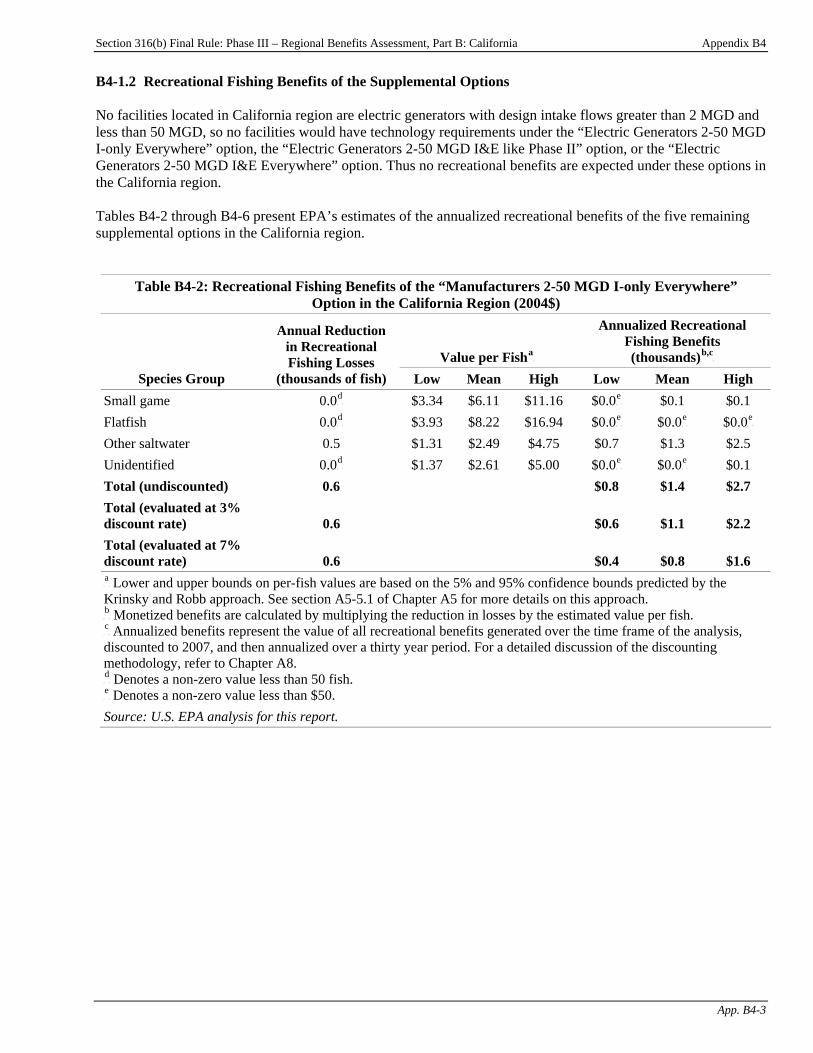
Section 316(b) Final Rule: Phase III – Regional Benefits Assessment, Part B: California Appendix B4
App. B4-3
B4-1.2 Recreational Fishing Benefits of the Supplemental Options No facilities located in California region are electric generators with design intake flows greater than 2 MGD and less than 50 MGD, so no facilities would have technology requirements under the “Electric Generators 2-50 MGD I-only Everywhere” option, the “Electric Generators 2-50 MGD I&E like Phase II” option, or the “Electric Generators 2-50 MGD I&E Everywhere” option. Thus no recreational benefits are expected under these options in the California region. Tables B4-2 through B4-6 present EPA’s estimates of the annualized recreational benefits of the five remaining supplemental options in the California region.
Table B4-2: Recreational Fishing Benefits of the “Manufacturers 2-50 MGD I-only Everywhere” Option in the California Region (2004$)
Value per FishP
aP
Annualized Recreational Fishing Benefits (thousands)P
b,cP
Species Group
Annual Reduction in Recreational Fishing Losses
(thousands of fish) Low Mean High Low Mean High Small game 0.0P
dP $3.34 $6.11 $11.16 $0.0P
eP $0.1 $0.1
Flatfish 0.0P
dP $3.93 $8.22 $16.94 $0.0P
eP $0.0P
eP $0.0P
eP
Other saltwater 0.5 $1.31 $2.49 $4.75 $0.7 $1.3 $2.5 Unidentified 0.0P
dP $1.37 $2.61 $5.00 $0.0P
eP $0.0P
eP $0.1
Total (undiscounted) 0.6 $0.8 $1.4 $2.7 Total (evaluated at 3% discount rate) 0.6 $0.6 $1.1 $2.2 Total (evaluated at 7% discount rate) 0.6 $0.4 $0.8 $1.6 P
aP Lower and upper bounds on per-fish values are based on the 5% and 95% confidence bounds predicted by the
Krinsky and Robb approach. See section A5-5.1 of Chapter A5 for more details on this approach. P
bP Monetized benefits are calculated by multiplying the reduction in losses by the estimated value per fish.
P
cP Annualized benefits represent the value of all recreational benefits generated over the time frame of the analysis,
discounted to 2007, and then annualized over a thirty year period. For a detailed discussion of the discounting methodology, refer to Chapter A8. P
dP Denotes a non-zero value less than 50 fish.
P
eP Denotes a non-zero value less than $50.
Source: U.S. EPA analysis for this report.

Section 316(b) Final Rule: Phase III – Regional Benefits Assessment, Part B: California Appendix B4
App. B4-4
Table B4-3: Recreational Fishing Benefits of the “Manufacturers 2-50 MGD I&E like Phase II” Option in the California Region (2004$)
Value per FishP
aP
Annualized Recreational Fishing Benefits (thousands)P
b,cP
Species Group
Annual Reduction in Recreational Fishing Losses
(thousands of fish) Low Mean High Low Mean High Small game 0.0P
dP $3.34 $6.11 $11.16 $0.0P
eP $0.1 $0.1
Flatfish 0.2 $3.93 $8.22 $16.94 $0.7 $1.6 $3.2 Other saltwater 9.1 $1.31 $2.49 $4.75 $11.9 $22.6 $43.0 Unidentified 0.0P
dP $1.37 $2.61 $5.00 $0.1 $0.1 $0.2
Total (undiscounted) 9.3 $12.7 $24.3 $46.6 Total (evaluated at 3% discount rate)P
cP 9.3 $10.0 $19.2 $36.7
Total (evaluated at 7% discount rate)P
cP 9.3 $7.4 $14.1 $27.1
P
aP Lower and upper bounds on per-fish values are based on the 5% and 95% confidence bounds predicted by the
Krinsky and Robb approach. See section A5-5.1 of Chapter A5 for more details on this approach. P
bP Monetized benefits are calculated by multiplying the reduction in losses by the estimated value per fish.
P
cP Annualized benefits represent the value of all recreational benefits generated over the time frame of the analysis,
discounted to 2007, and then annualized over a thirty year period. For a detailed discussion of the discounting methodology, refer to Chapter A8. P
dP Denotes a non-zero value less than 50 fish.
P
eP Denotes a non-zero value less than $50.
Source: U.S. EPA analysis for this report.
Table B4-4: Recreational Fishing Benefits of the “Manufacturers 2-50 MGD I&E Everywhere” Option in the California Region (2004$)
Value per FishP
aP
Annualized Recreational Fishing Benefits (thousands)P
b,cP
Species Group
Annual Reduction in Recreational Fishing Losses
(thousands of fish) Low Mean High Low Mean High Small game 0.0P
dP $3.34 $6.11 $11.16 $0.0P
eP $0.1 $0.1
Flatfish 0.2 $3.93 $8.22 $16.94 $0.8 $1.7 $3.6 Other saltwater 10.0 $1.31 $2.49 $4.75 $13.1 $25.0 $47.6 Unidentified 0.0P
dP $1.37 $2.61 $5.00 $0.1 $0.1 $0.2
Total (undiscounted) 10.3 $14.1 $26.9 $51.5 Total (evaluated at 3% discount rate)P
cP 10.3 $11.1 $21.2 $40.6
Total (evaluated at 7% discount rate)P
cP 10.3 $8.2 $15.6 $30.0
P
aP Lower and upper bounds on per-fish values are based on the 5% and 95% confidence bounds predicted by the
Krinsky and Robb approach. See section A5-5.1 of Chapter A5 for more details on this approach. P
bP Monetized benefits are calculated by multiplying the reduction in losses by the estimated value per fish.
P
cP Annualized benefits represent the value of all recreational benefits generated over the time frame of the analysis,
discounted to 2007, and then annualized over a thirty year period. For a detailed discussion of the discounting methodology, refer to Chapter A8. P
dP Denotes a non-zero value less than 50 fish.
P
eP Denotes a non-zero value less than $50.
Source: U.S. EPA analysis for this report.

Section 316(b) Final Rule: Phase III – Regional Benefits Assessment, Part B: California Appendix B4
App. B4-5
Table B4-5: Recreational Fishing Benefits of the “Manufacturers 50+ MGD I-only Everywhere” Option in the California Region (2004$)
Value per FishP
aP
Annualized Recreational Fishing Benefits (thousands)P
b,cP
Species Group
Annual Reduction in Recreational Fishing Losses
(thousands of fish) Low Mean High Low Mean High Small game 0.0P
dP $3.34 $6.11 $11.16 $0.0P
eP $0.1 $0.1
Flatfish 0.0P
dP $3.93 $8.22 $16.94 $0.0P
eP $0.0P
eP $0.0P
eP
Other saltwater 0.5 $1.31 $2.49 $4.75 $0.7 $1.3 $2.5 Unidentified 0.0P
dP $1.37 $2.61 $5.00 $0.0P
eP $0.0P
eP $0.1
Total (undiscounted) 0.6 $0.7 $1.4 $2.7 Total (evaluated at 3% discount rate)P
cP 0.6 $0.6 $1.2 $2.3
Total (evaluated at 7% discount rate)P
cP 0.6 $0.5 $1.0 $1.9
P
aP Lower and upper bounds on per-fish values are based on the 5% and 95% confidence bounds predicted by the
Krinsky and Robb approach. See section A5-5.1 of Chapter A5 for more details on this approach. P
bP Monetized benefits are calculated by multiplying the reduction in losses by the estimated value per fish.
P
cP Annualized benefits represent the value of all recreational benefits generated over the time frame of the analysis,
discounted to 2007, and then annualized over a thirty year period. For a detailed discussion of the discounting methodology, refer to Chapter A8. P
dP Denotes a non-zero value less than 50 fish.
P
eP Denotes a non-zero value less than $50.
Source: U.S. EPA analysis for this report.
Table B4-6: Recreational Fishing Benefits of the “Manufacturers 50+ MGD I&E Everywhere” Option in the California Region (2004$)
Value per FishP
aP
Annualized Recreational Fishing Benefits (thousands)P
b,cP
Species Group
Annual Reduction in Recreational Fishing Losses
(thousands of fish) Low Mean High Low Mean High Small game 0.0P
dP $3.34 $6.11 $11.16 $0.0P
eP $0.1 $0.1
Flatfish 0.2 $3.93 $8.22 $16.94 $0.7 $1.5 $3.2 Other saltwater 8.9 $1.31 $2.49 $4.75 $11.7 $22.3 $42.4 Unidentified 0.0P
dP $1.37 $2.61 $5.00 $0.1 $0.1 $0.2
Total (undiscounted) 9.2 $12.5 $24.0 $45.9 Total (evaluated at 3% discount rate) 9.2 $10.8 $20.7 $39.6 Total (evaluated at 7% discount rate) 9.2 $8.9 $17.1 $32.7 P
aP Lower and upper bounds on per-fish values are based on the 5% and 95% confidence bounds predicted by the
Krinsky and Robb approach. See section A5-5.1 of Chapter A5 for more details on this approach. P
bP Monetized benefits are calculated by multiplying the reduction in losses by the estimated value per fish.
P
cP Annualized benefits represent the value of all recreational benefits generated over the time frame of the analysis,
discounted to 2007, and then annualized over a thirty year period. For a detailed discussion of the discounting methodology, refer to Chapter A8. P
dP Denotes a non-zero value less than 50 fish.
P
eP Denotes a non-zero value less than $50.
Source: U.S. EPA analysis for this report.
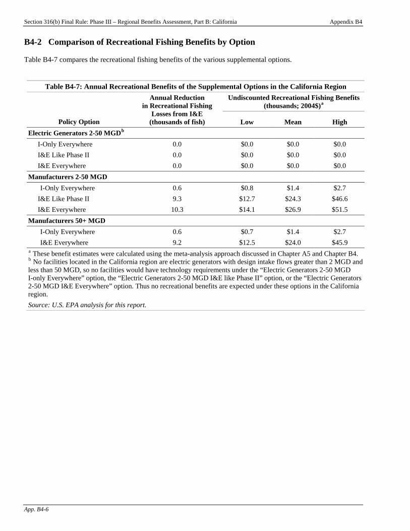
Section 316(b) Final Rule: Phase III – Regional Benefits Assessment, Part B: California Appendix B4
App. B4-6
B4-2 Comparison of Recreational Fishing Benefits by Option Table B4-7 compares the recreational fishing benefits of the various supplemental options.
Table B4-7: Annual Recreational Benefits of the Supplemental Options in the California Region Undiscounted Recreational Fishing Benefits
(thousands; 2004$)P
aP
Policy Option
Annual Reduction in Recreational Fishing
Losses from I&E (thousands of fish) Low Mean High
Electric Generators 2-50 MGDP
bP
I-Only Everywhere 0.0 $0.0 $0.0 $0.0 I&E Like Phase II 0.0 $0.0 $0.0 $0.0 I&E Everywhere 0.0 $0.0 $0.0 $0.0
Manufacturers 2-50 MGD I-Only Everywhere 0.6 $0.8 $1.4 $2.7
I&E Like Phase II 9.3 $12.7 $24.3 $46.6 I&E Everywhere 10.3 $14.1 $26.9 $51.5
Manufacturers 50+ MGD I-Only Everywhere 0.6 $0.7 $1.4 $2.7 I&E Everywhere 9.2 $12.5 $24.0 $45.9
P
aP These benefit estimates were calculated using the meta-analysis approach discussed in Chapter A5 and Chapter B4.
P
bP No facilities located in the California region are electric generators with design intake flows greater than 2 MGD and
less than 50 MGD, so no facilities would have technology requirements under the “Electric Generators 2-50 MGD I-only Everywhere” option, the “Electric Generators 2-50 MGD I&E like Phase II” option, or the “Electric Generators 2-50 MGD I&E Everywhere” option. Thus no recreational benefits are expected under these options in the California region. Source: U.S. EPA analysis for this report.
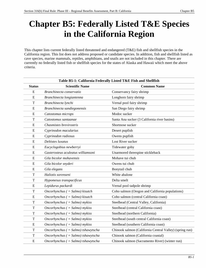
Section 316(b) Final Rule: Phase III – Regional Benefits Assessment, Part B: California Chapter B5
B5-1
Chapter B5: Federally Listed T&E Species in the California Region
This chapter lists current federally listed threatened and endangered (T&E) fish and shellfish species in the California region. This list does not address proposed or candidate species. In addition, fish and shellfish listed as cave species, marine mammals, reptiles, amphibians, and snails are not included in this chapter. There are currently no federally listed fish or shellfish species for the states of Alaska and Hawaii which meet the above criteria.
Table B5-1: California Federally Listed T&E Fish and Shellfish Status Scientific Name Common Name
E Branchinecta conservatio Conservancy fairy shrimp E Branchinecta longiantenna Longhorn fairy shrimp T Branchinecta lynchi Vernal pool fairy shrimp E Branchinecta sandiegonensis San Diego fairy shrimp E Catostomus microps Modoc sucker T Catostomus santaanae Santa Ana sucker (3 California river basins) E Chasmistes brevirostris Shortnose sucker E Cyprinodon macularius Desert pupfish E Cyprinodon radiosus Owens pupfish E Deltistes luxatus Lost River sucker E Eucyclogobius newberryi Tidewater goby E Gasterosteus aculeatus williamsoni Unarmored threespine stickleback E Gila bicolor mohavensis Mohave tui chub E Gila bicolor snyderi Owens tui chub E Gila elegans Bonytail chub T Haliotis sorenseni White abalone T Hypomesus transpacificus Delta smelt E Lepidurus packardi Vernal pool tadpole shrimp T Oncorhynchus ( = Salmo) kisutch Coho salmon (Oregon and California populations) E Oncorhynchus ( = Salmo) kisutch Coho salmon (central California coast) T Oncorhynchus ( = Salmo) mykiss Steelhead (Central Valley, California) T Oncorhynchus ( = Salmo) mykiss Steelhead (central California coast) T Oncorhynchus ( = Salmo) mykiss Steelhead (northern California) T Oncorhynchus ( = Salmo) mykiss Steelhead (south central California coast) E Oncorhynchus ( = Salmo) mykiss Steelhead (southern California coast) T Oncorhynchus ( = Salmo) tshawytscha Chinook salmon (California Central Valley) (spring run) T Oncorhynchus ( = Salmo) tshawytscha Chinook salmon (California coastal) E Oncorhynchus ( = Salmo) tshawytscha Chinook salmon (Sacramento River) (winter run)
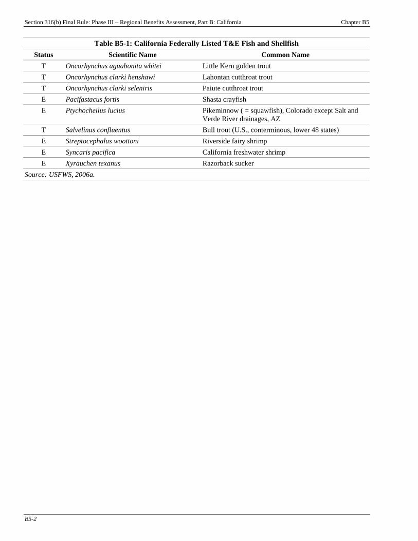
Section 316(b) Final Rule: Phase III – Regional Benefits Assessment, Part B: California Chapter B5
B5-2
Table B5-1: California Federally Listed T&E Fish and Shellfish Status Scientific Name Common Name
T Oncorhynchus aguabonita whitei Little Kern golden trout T Oncorhynchus clarki henshawi Lahontan cutthroat trout T Oncorhynchus clarki seleniris Paiute cutthroat trout E Pacifastacus fortis Shasta crayfish E Ptychocheilus lucius Pikeminnow ( = squawfish), Colorado except Salt and
Verde River drainages, AZ T Salvelinus confluentus Bull trout (U.S., conterminous, lower 48 states) E Streptocephalus woottoni Riverside fairy shrimp E Syncaris pacifica California freshwater shrimp E Xyrauchen texanus Razorback sucker
Source: USFWS, 2006a.

Section 316(b) Final Rule: Phase III – Regional Benefits Assessment
Part C: North Atlantic
Section 316(b) Final Rule: Phase III – Regional Benefits Assessment, Part C: North Atlantic Chapter C1
C1-1
Chapter C1: Background Introduction This chapter presents an overview of the potential Phase III existing facilities in the North Atlantic study region and summarizes their key cooling water and compliance characteristics. For further discussion of the technical and compliance characteristics of potential Phase III existing facilities, refer to the Economic Analysis for the Final Section 316(b) Rule for Phase III Facilities and the Technical Development Document for the Final Section 316(b) Rule for Phase III Facilities (U.S. EPA, 2006a,c).
Chapter Contents C1-1 Facility Characteristics..................................C1-1
C1-1 Facility Characteristics The North Atlantic Regional Study includes four sample facilities that are potentially subject to the national standards for Phase III existing facilities. Figure C1-1 presents a map of these facilities. All four facilities are manufacturing facilities. Industry-wide, these four sample facilities represent five manufacturing facilities.PF
1FP
P
1P EPA applied sample weights to the survey respondents to account for non-sampled facilities and facilities that did
not respond to the survey. For more information on EPA’s 2000 Section 316(b) Industry Survey, please refer to the Information Collection Request (U.S. EPA, 2000b).
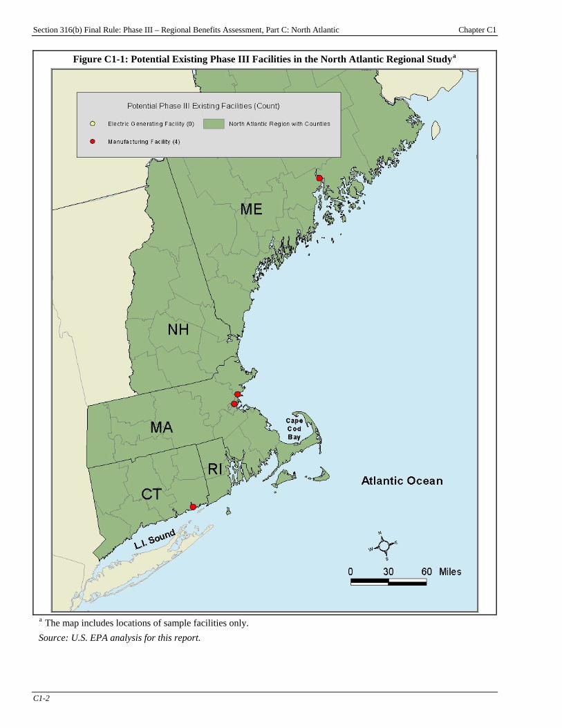
Section 316(b) Final Rule: Phase III – Regional Benefits Assessment, Part C: North Atlantic Chapter C1
C1-2
Figure C1-1: Potential Existing Phase III Facilities in the North Atlantic Regional StudyP
aP
P
aP The map includes locations of sample facilities only.
Source: U.S. EPA analysis for this report.
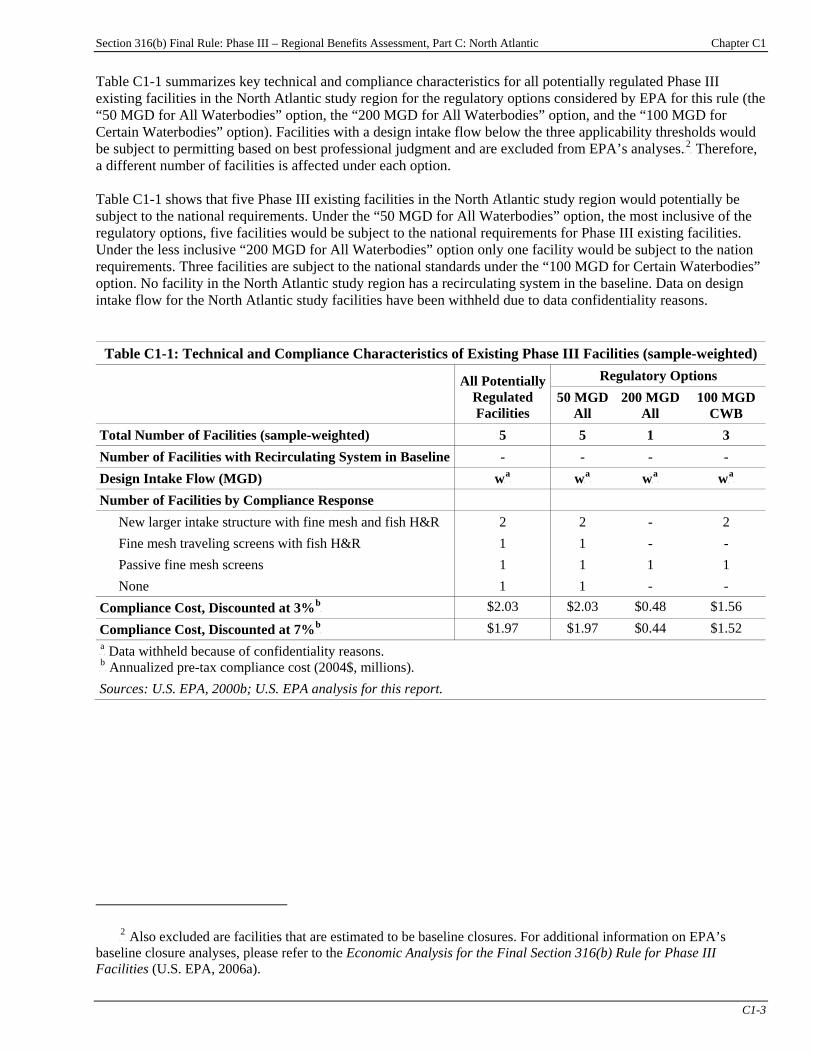
Section 316(b) Final Rule: Phase III – Regional Benefits Assessment, Part C: North Atlantic Chapter C1
C1-3
Table C1-1 summarizes key technical and compliance characteristics for all potentially regulated Phase III existing facilities in the North Atlantic study region for the regulatory options considered by EPA for this rule (the “50 MGD for All Waterbodies” option, the “200 MGD for All Waterbodies” option, and the “100 MGD for Certain Waterbodies” option). Facilities with a design intake flow below the three applicability thresholds would be subject to permitting based on best professional judgment and are excluded from EPA’s analyses.PF
2FP Therefore,
a different number of facilities is affected under each option. Table C1-1 shows that five Phase III existing facilities in the North Atlantic study region would potentially be subject to the national requirements. Under the “50 MGD for All Waterbodies” option, the most inclusive of the regulatory options, five facilities would be subject to the national requirements for Phase III existing facilities. Under the less inclusive “200 MGD for All Waterbodies” option only one facility would be subject to the nation requirements. Three facilities are subject to the national standards under the “100 MGD for Certain Waterbodies” option. No facility in the North Atlantic study region has a recirculating system in the baseline. Data on design intake flow for the North Atlantic study facilities have been withheld due to data confidentiality reasons.
Table C1-1: Technical and Compliance Characteristics of Existing Phase III Facilities (sample-weighted) Regulatory Options All Potentially
Regulated Facilities
50 MGD All
200 MGD All
100 MGD CWB
Total Number of Facilities (sample-weighted) 5 5 1 3 Number of Facilities with Recirculating System in Baseline - - - - Design Intake Flow (MGD) wP
aP wP
aP wP
aP wP
aP
Number of Facilities by Compliance Response New larger intake structure with fine mesh and fish H&R 2 2 - 2 Fine mesh traveling screens with fish H&R 1 1 - - Passive fine mesh screens 1 1 1 1 None 1 1 - -
Compliance Cost, Discounted at 3%P
bP
$2.03 $2.03 $0.48 $1.56
Compliance Cost, Discounted at 7%P
bP
$1.97 $1.97 $0.44 $1.52 P
aP Data withheld because of confidentiality reasons.
P
bP Annualized pre-tax compliance cost (2004$, millions).
Sources: U.S. EPA, 2000b; U.S. EPA analysis for this report.
P
2P Also excluded are facilities that are estimated to be baseline closures. For additional information on EPA’s
baseline closure analyses, please refer to the Economic Analysis for the Final Section 316(b) Rule for Phase III Facilities (U.S. EPA, 2006a).
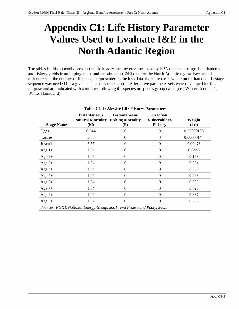
Section 316(b) Final Rule: Phase III – Regional Benefits Assessment, Part C: North Atlantic Appendix C1
App. C1-1
Appendix C1: Life History Parameter Values Used to Evaluate I&E in the
North Atlantic Region The tables in this appendix present the life history parameter values used by EPA to calculate age-1 equivalents and fishery yields from impingement and entrainment (I&E) data for the North Atlantic region. Because of differences in the number of life stages represented in the loss data, there are cases where more than one life stage sequence was needed for a given species or species group. Alternative parameter sets were developed for this purpose and are indicated with a number following the species or species group name (i.e., Winter flounder 1, Winter flounder 2).
Table C1-1: Alewife Life History Parameters
Stage Name
Instantaneous Natural Mortality
(M)
Instantaneous Fishing Mortality
(F)
Fraction Vulnerable to
Fishery Weight
(lbs) Eggs 0.544 0 0 0.00000128 Larvae 5.50 0 0 0.00000141 Juvenile 2.57 0 0 0.00478 Age 1+ 1.04 0 0 0.0443 Age 2+ 1.04 0 0 0.139 Age 3+ 1.04 0 0 0.264 Age 4+ 1.04 0 0 0.386 Age 5+ 1.04 0 0 0.489 Age 6+ 1.04 0 0 0.568 Age 7+ 1.04 0 0 0.626 Age 8+ 1.04 0 0 0.667 Age 9+ 1.04 0 0 0.696 Sources: PG&E National Energy Group, 2001; and Froese and Pauly, 2003.
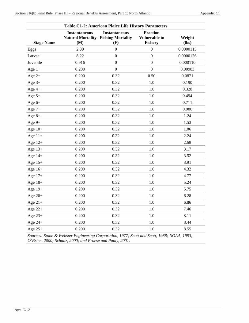
Section 316(b) Final Rule: Phase III – Regional Benefits Assessment, Part C: North Atlantic Appendix C1
App. C1-2
Table C1-2: American Plaice Life History Parameters
Stage Name
Instantaneous Natural Mortality
(M)
Instantaneous Fishing Mortality
(F)
Fraction Vulnerable to
Fishery Weight
(lbs) Eggs 2.30 0 0 0.0000115 Larvae 8.22 0 0 0.0000126 Juvenile 0.916 0 0 0.000110 Age 1+ 0.200 0 0 0.00903 Age 2+ 0.200 0.32 0.50 0.0871 Age 3+ 0.200 0.32 1.0 0.190 Age 4+ 0.200 0.32 1.0 0.328 Age 5+ 0.200 0.32 1.0 0.494 Age 6+ 0.200 0.32 1.0 0.711 Age 7+ 0.200 0.32 1.0 0.986 Age 8+ 0.200 0.32 1.0 1.24 Age 9+ 0.200 0.32 1.0 1.53 Age 10+ 0.200 0.32 1.0 1.86 Age 11+ 0.200 0.32 1.0 2.24 Age 12+ 0.200 0.32 1.0 2.68 Age 13+ 0.200 0.32 1.0 3.17 Age 14+ 0.200 0.32 1.0 3.52 Age 15+ 0.200 0.32 1.0 3.91 Age 16+ 0.200 0.32 1.0 4.32 Age 17+ 0.200 0.32 1.0 4.77 Age 18+ 0.200 0.32 1.0 5.24 Age 19+ 0.200 0.32 1.0 5.75 Age 20+ 0.200 0.32 1.0 6.28 Age 21+ 0.200 0.32 1.0 6.86 Age 22+ 0.200 0.32 1.0 7.46 Age 23+ 0.200 0.32 1.0 8.11 Age 24+ 0.200 0.32 1.0 8.44 Age 25+ 0.200 0.32 1.0 8.55 Sources: Stone & Webster Engineering Corporation, 1977; Scott and Scott, 1988; NOAA, 1993; O’Brien, 2000; Schultz, 2000; and Froese and Pauly, 2001.
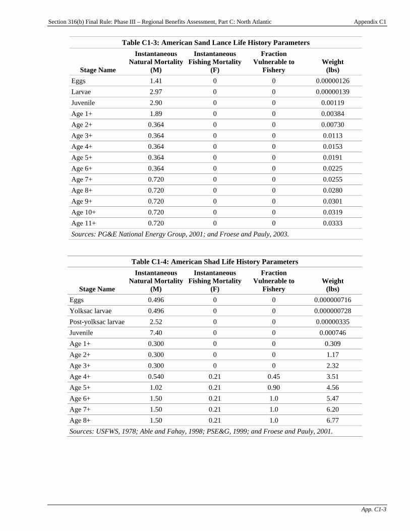
Section 316(b) Final Rule: Phase III – Regional Benefits Assessment, Part C: North Atlantic Appendix C1
App. C1-3
Table C1-3: American Sand Lance Life History Parameters
Stage Name
Instantaneous Natural Mortality
(M)
Instantaneous Fishing Mortality
(F)
Fraction Vulnerable to
Fishery Weight
(lbs) Eggs 1.41 0 0 0.00000126 Larvae 2.97 0 0 0.00000139 Juvenile 2.90 0 0 0.00119 Age 1+ 1.89 0 0 0.00384 Age 2+ 0.364 0 0 0.00730 Age 3+ 0.364 0 0 0.0113 Age 4+ 0.364 0 0 0.0153 Age 5+ 0.364 0 0 0.0191 Age 6+ 0.364 0 0 0.0225 Age 7+ 0.720 0 0 0.0255 Age 8+ 0.720 0 0 0.0280 Age 9+ 0.720 0 0 0.0301 Age 10+ 0.720 0 0 0.0319 Age 11+ 0.720 0 0 0.0333 Sources: PG&E National Energy Group, 2001; and Froese and Pauly, 2003.
Table C1-4: American Shad Life History Parameters
Stage Name
Instantaneous Natural Mortality
(M)
Instantaneous Fishing Mortality
(F)
Fraction Vulnerable to
Fishery Weight
(lbs) Eggs 0.496 0 0 0.000000716 Yolksac larvae 0.496 0 0 0.000000728 Post-yolksac larvae 2.52 0 0 0.00000335 Juvenile 7.40 0 0 0.000746 Age 1+ 0.300 0 0 0.309 Age 2+ 0.300 0 0 1.17 Age 3+ 0.300 0 0 2.32 Age 4+ 0.540 0.21 0.45 3.51 Age 5+ 1.02 0.21 0.90 4.56 Age 6+ 1.50 0.21 1.0 5.47 Age 7+ 1.50 0.21 1.0 6.20 Age 8+ 1.50 0.21 1.0 6.77 Sources: USFWS, 1978; Able and Fahay, 1998; PSE&G, 1999; and Froese and Pauly, 2001.
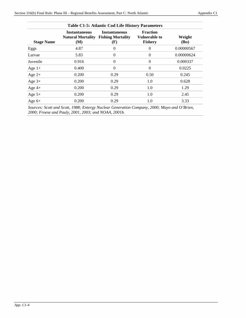
Section 316(b) Final Rule: Phase III – Regional Benefits Assessment, Part C: North Atlantic Appendix C1
App. C1-4
Table C1-5: Atlantic Cod Life History Parameters
Stage Name
Instantaneous Natural Mortality
(M)
Instantaneous Fishing Mortality
(F)
Fraction Vulnerable to
Fishery Weight
(lbs) Eggs 4.87 0 0 0.00000567 Larvae 5.83 0 0 0.00000624 Juvenile 0.916 0 0 0.000337 Age 1+ 0.400 0 0 0.0225 Age 2+ 0.200 0.29 0.50 0.245 Age 3+ 0.200 0.29 1.0 0.628 Age 4+ 0.200 0.29 1.0 1.29 Age 5+ 0.200 0.29 1.0 2.45 Age 6+ 0.200 0.29 1.0 3.33 Sources: Scott and Scott, 1988; Entergy Nuclear Generation Company, 2000; Mayo and O’Brien, 2000; Froese and Pauly, 2001, 2003; and NOAA, 2001b.
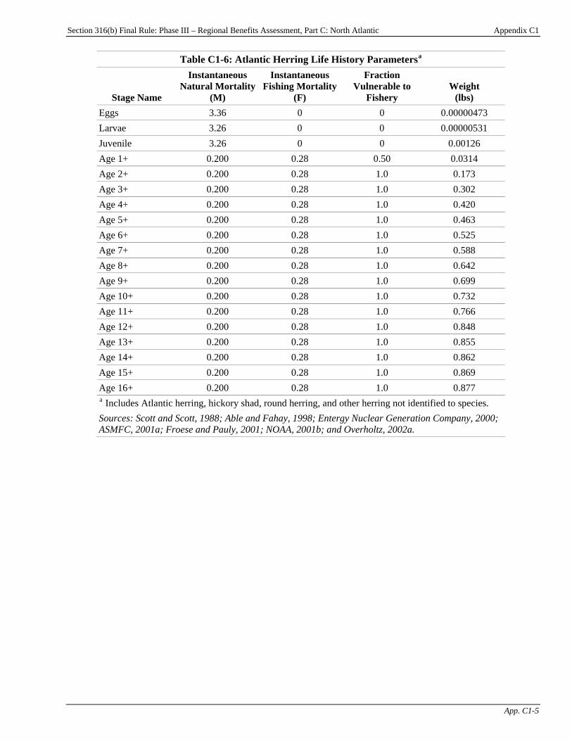
Section 316(b) Final Rule: Phase III – Regional Benefits Assessment, Part C: North Atlantic Appendix C1
App. C1-5
Table C1-6: Atlantic Herring Life History ParametersP
aP
Stage Name
Instantaneous Natural Mortality
(M)
Instantaneous Fishing Mortality
(F)
Fraction Vulnerable to
Fishery Weight
(lbs) Eggs 3.36 0 0 0.00000473 Larvae 3.26 0 0 0.00000531 Juvenile 3.26 0 0 0.00126 Age 1+ 0.200 0.28 0.50 0.0314 Age 2+ 0.200 0.28 1.0 0.173 Age 3+ 0.200 0.28 1.0 0.302 Age 4+ 0.200 0.28 1.0 0.420 Age 5+ 0.200 0.28 1.0 0.463 Age 6+ 0.200 0.28 1.0 0.525 Age 7+ 0.200 0.28 1.0 0.588 Age 8+ 0.200 0.28 1.0 0.642 Age 9+ 0.200 0.28 1.0 0.699 Age 10+ 0.200 0.28 1.0 0.732 Age 11+ 0.200 0.28 1.0 0.766 Age 12+ 0.200 0.28 1.0 0.848 Age 13+ 0.200 0.28 1.0 0.855 Age 14+ 0.200 0.28 1.0 0.862 Age 15+ 0.200 0.28 1.0 0.869 Age 16+ 0.200 0.28 1.0 0.877 P
aP Includes Atlantic herring, hickory shad, round herring, and other herring not identified to species.
Sources: Scott and Scott, 1988; Able and Fahay, 1998; Entergy Nuclear Generation Company, 2000; ASMFC, 2001a; Froese and Pauly, 2001; NOAA, 2001b; and Overholtz, 2002a.
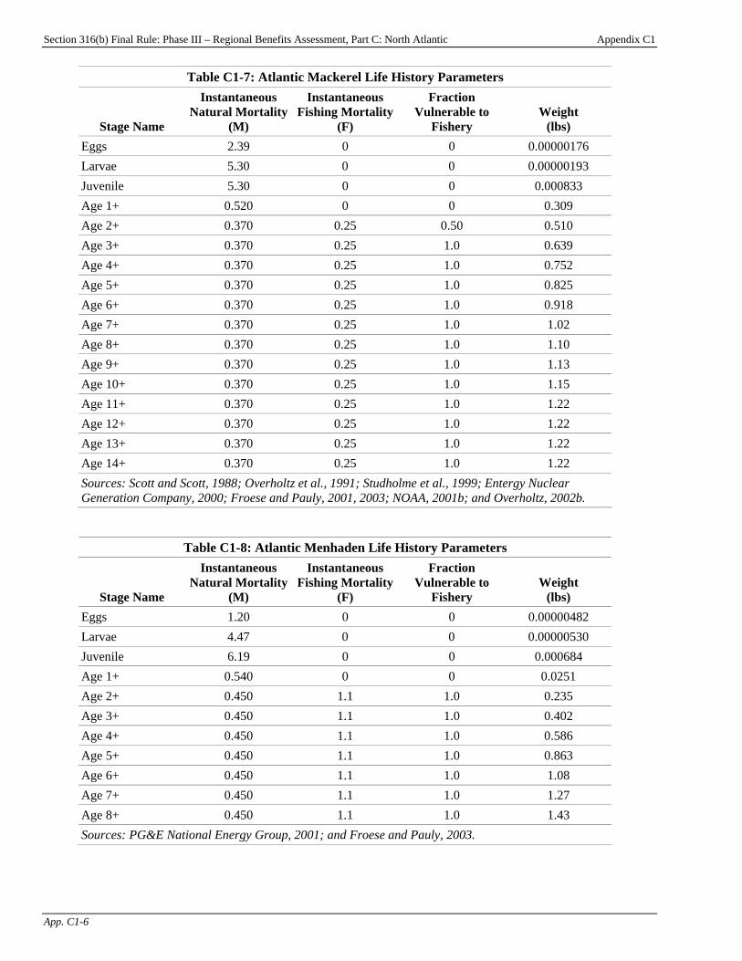
Section 316(b) Final Rule: Phase III – Regional Benefits Assessment, Part C: North Atlantic Appendix C1
App. C1-6
Table C1-7: Atlantic Mackerel Life History Parameters
Stage Name
Instantaneous Natural Mortality
(M)
Instantaneous Fishing Mortality
(F)
Fraction Vulnerable to
Fishery Weight
(lbs) Eggs 2.39 0 0 0.00000176 Larvae 5.30 0 0 0.00000193 Juvenile 5.30 0 0 0.000833 Age 1+ 0.520 0 0 0.309 Age 2+ 0.370 0.25 0.50 0.510 Age 3+ 0.370 0.25 1.0 0.639 Age 4+ 0.370 0.25 1.0 0.752 Age 5+ 0.370 0.25 1.0 0.825 Age 6+ 0.370 0.25 1.0 0.918 Age 7+ 0.370 0.25 1.0 1.02 Age 8+ 0.370 0.25 1.0 1.10 Age 9+ 0.370 0.25 1.0 1.13 Age 10+ 0.370 0.25 1.0 1.15 Age 11+ 0.370 0.25 1.0 1.22 Age 12+ 0.370 0.25 1.0 1.22 Age 13+ 0.370 0.25 1.0 1.22 Age 14+ 0.370 0.25 1.0 1.22 Sources: Scott and Scott, 1988; Overholtz et al., 1991; Studholme et al., 1999; Entergy Nuclear Generation Company, 2000; Froese and Pauly, 2001, 2003; NOAA, 2001b; and Overholtz, 2002b.
Table C1-8: Atlantic Menhaden Life History Parameters
Stage Name
Instantaneous Natural Mortality
(M)
Instantaneous Fishing Mortality
(F)
Fraction Vulnerable to
Fishery Weight
(lbs) Eggs 1.20 0 0 0.00000482 Larvae 4.47 0 0 0.00000530 Juvenile 6.19 0 0 0.000684 Age 1+ 0.540 0 0 0.0251 Age 2+ 0.450 1.1 1.0 0.235 Age 3+ 0.450 1.1 1.0 0.402 Age 4+ 0.450 1.1 1.0 0.586 Age 5+ 0.450 1.1 1.0 0.863 Age 6+ 0.450 1.1 1.0 1.08 Age 7+ 0.450 1.1 1.0 1.27 Age 8+ 0.450 1.1 1.0 1.43 Sources: PG&E National Energy Group, 2001; and Froese and Pauly, 2003.
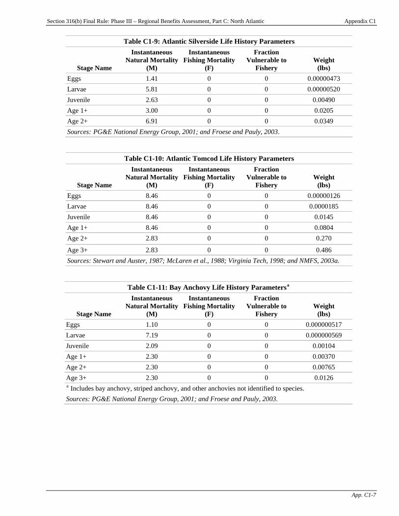
Section 316(b) Final Rule: Phase III – Regional Benefits Assessment, Part C: North Atlantic Appendix C1
App. C1-7
Table C1-9: Atlantic Silverside Life History Parameters
Stage Name
Instantaneous Natural Mortality
(M)
Instantaneous Fishing Mortality
(F)
Fraction Vulnerable to
Fishery Weight
(lbs) Eggs 1.41 0 0 0.00000473 Larvae 5.81 0 0 0.00000520 Juvenile 2.63 0 0 0.00490 Age 1+ 3.00 0 0 0.0205 Age 2+ 6.91 0 0 0.0349 Sources: TPG&E National Energy Group, 2001; and Froese and Pauly, 2003T.
Table C1-10: Atlantic Tomcod Life History Parameters
Stage Name
Instantaneous Natural Mortality
(M)
Instantaneous Fishing Mortality
(F)
Fraction Vulnerable to
Fishery Weight
(lbs) Eggs 8.46 0 0 0.00000126 Larvae 8.46 0 0 0.0000185 Juvenile 8.46 0 0 0.0145 Age 1+ 8.46 0 0 0.0804 Age 2+ 2.83 0 0 0.270
Age 3+ 2.83 0 0 0.486 Sources: Stewart and Auster, 1987; McLaren et al., 1988; Virginia Tech, 1998; and NMFS, 2003a.
Table C1-11: Bay Anchovy Life History ParametersP
aP
Stage Name
Instantaneous Natural Mortality
(M)
Instantaneous Fishing Mortality
(F)
Fraction Vulnerable to
Fishery Weight
(lbs) Eggs 1.10 0 0 0.000000517 Larvae 7.19 0 0 0.000000569 Juvenile 2.09 0 0 0.00104 Age 1+ 2.30 0 0 0.00370 Age 2+ 2.30 0 0 0.00765 Age 3+ 2.30 0 0 0.0126 P
aP Includes bay anchovy, striped anchovy, and other anchovies not identified to species.
Sources: PG&E National Energy Group, 2001; and Froese and Pauly, 2003.
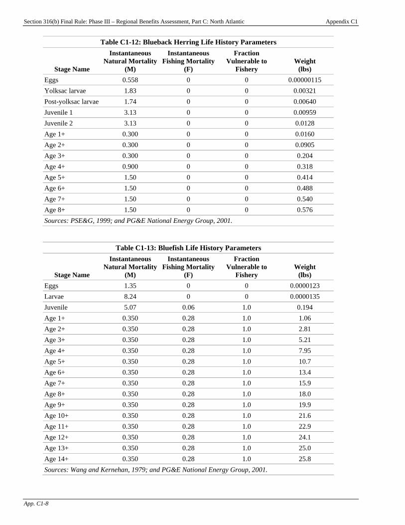
Section 316(b) Final Rule: Phase III – Regional Benefits Assessment, Part C: North Atlantic Appendix C1
App. C1-8
Table C1-12: Blueback Herring Life History Parameters
Stage Name
Instantaneous Natural Mortality
(M)
Instantaneous Fishing Mortality
(F)
Fraction Vulnerable to
Fishery Weight
(lbs) Eggs 0.558 0 0 0.00000115 Yolksac larvae 1.83 0 0 0.00321 Post-yolksac larvae 1.74 0 0 0.00640 Juvenile 1 3.13 0 0 0.00959 Juvenile 2 3.13 0 0 0.0128 Age 1+ 0.300 0 0 0.0160 Age 2+ 0.300 0 0 0.0905 Age 3+ 0.300 0 0 0.204 Age 4+ 0.900 0 0 0.318 Age 5+ 1.50 0 0 0.414 Age 6+ 1.50 0 0 0.488 Age 7+ 1.50 0 0 0.540 Age 8+ 1.50 0 0 0.576 Sources: PSE&G, 1999; and PG&E National Energy Group, 2001.
Table C1-13: Bluefish Life History Parameters
Stage Name
Instantaneous Natural Mortality
(M)
Instantaneous Fishing Mortality
(F)
Fraction Vulnerable to
Fishery Weight
(lbs) Eggs 1.35 0 0 0.0000123 Larvae 8.24 0 0 0.0000135 Juvenile 5.07 0.06 1.0 0.194 Age 1+ 0.350 0.28 1.0 1.06 Age 2+ 0.350 0.28 1.0 2.81 Age 3+ 0.350 0.28 1.0 5.21 Age 4+ 0.350 0.28 1.0 7.95 Age 5+ 0.350 0.28 1.0 10.7 Age 6+ 0.350 0.28 1.0 13.4 Age 7+ 0.350 0.28 1.0 15.9 Age 8+ 0.350 0.28 1.0 18.0 Age 9+ 0.350 0.28 1.0 19.9 Age 10+ 0.350 0.28 1.0 21.6 Age 11+ 0.350 0.28 1.0 22.9 Age 12+ 0.350 0.28 1.0 24.1 Age 13+ 0.350 0.28 1.0 25.0 Age 14+ 0.350 0.28 1.0 25.8 Sources: Wang and Kernehan, 1979; and PG&E National Energy Group, 2001.
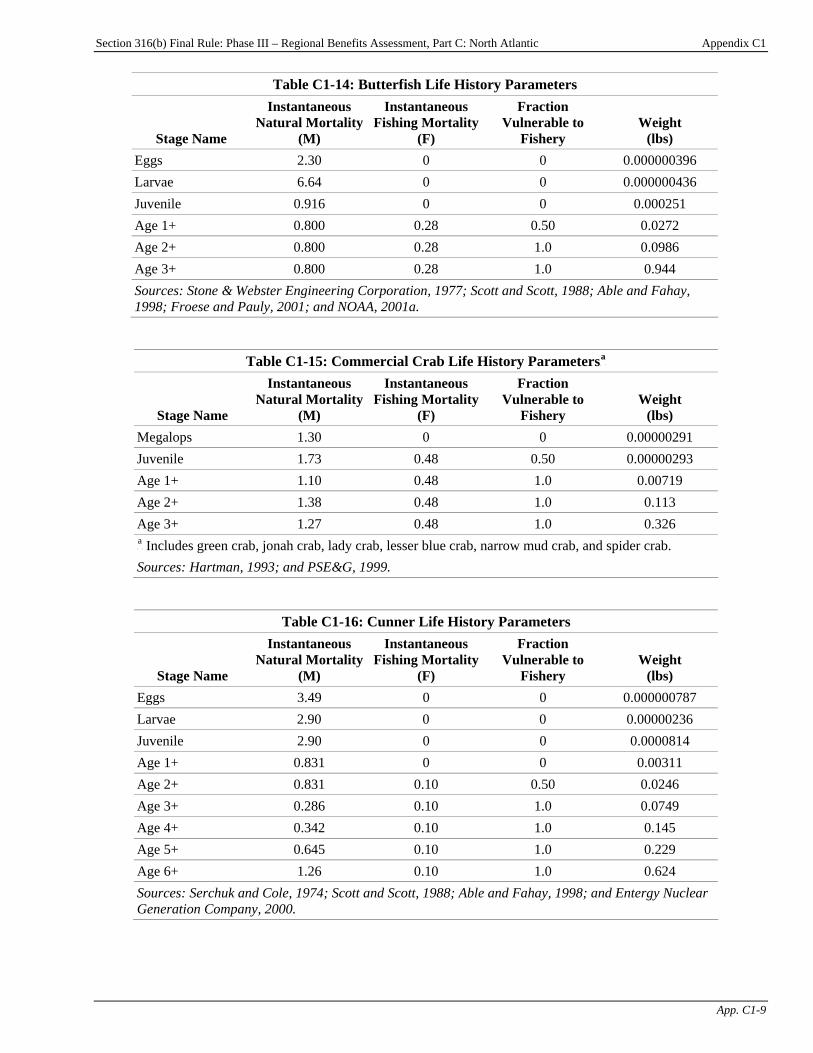
Section 316(b) Final Rule: Phase III – Regional Benefits Assessment, Part C: North Atlantic Appendix C1
App. C1-9
Table C1-14: Butterfish Life History Parameters
Stage Name
Instantaneous Natural Mortality
(M)
Instantaneous Fishing Mortality
(F)
Fraction Vulnerable to
Fishery Weight
(lbs) Eggs 2.30 0 0 0.000000396 Larvae 6.64 0 0 0.000000436 Juvenile 0.916 0 0 0.000251 Age 1+ 0.800 0.28 0.50 0.0272 Age 2+ 0.800 0.28 1.0 0.0986 Age 3+ 0.800 0.28 1.0 0.944 Sources: Stone & Webster Engineering Corporation, 1977; Scott and Scott, 1988; Able and Fahay, 1998; Froese and Pauly, 2001; and NOAA, 2001a.
Table C1-15: Commercial Crab Life History ParametersP
aP
Stage Name
Instantaneous Natural Mortality
(M)
Instantaneous Fishing Mortality
(F)
Fraction Vulnerable to
Fishery Weight
(lbs) Megalops 1.30 0 0 0.00000291 Juvenile 1.73 0.48 0.50 0.00000293 Age 1+ 1.10 0.48 1.0 0.00719 Age 2+ 1.38 0.48 1.0 0.113 Age 3+ 1.27 0.48 1.0 0.326 P
aP Includes green crab, jonah crab, lady crab, lesser blue crab, narrow mud crab, and spider crab.
Sources: Hartman, 1993; and PSE&G, 1999.
Table C1-16: Cunner Life History Parameters
Stage Name
Instantaneous Natural Mortality
(M)
Instantaneous Fishing Mortality
(F)
Fraction Vulnerable to
Fishery Weight
(lbs) Eggs 3.49 0 0 0.000000787 Larvae 2.90 0 0 0.00000236 Juvenile 2.90 0 0 0.0000814 Age 1+ 0.831 0 0 0.00311 Age 2+ 0.831 0.10 0.50 0.0246 Age 3+ 0.286 0.10 1.0 0.0749 Age 4+ 0.342 0.10 1.0 0.145 Age 5+ 0.645 0.10 1.0 0.229 Age 6+ 1.26 0.10 1.0 0.624 Sources: Serchuk and Cole, 1974; Scott and Scott, 1988; Able and Fahay, 1998; and Entergy Nuclear Generation Company, 2000.
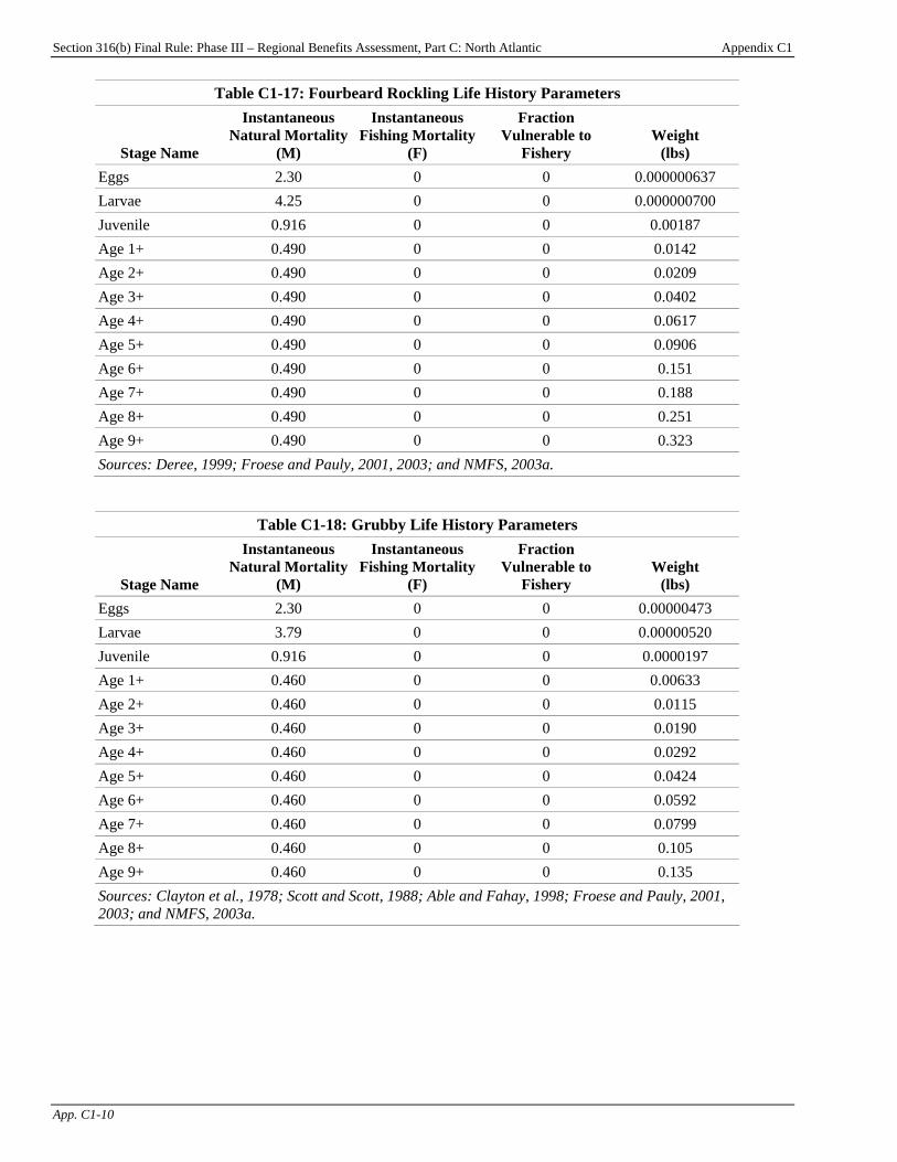
Section 316(b) Final Rule: Phase III – Regional Benefits Assessment, Part C: North Atlantic Appendix C1
App. C1-10
Table C1-17: Fourbeard Rockling Life History Parameters
Stage Name
Instantaneous Natural Mortality
(M)
Instantaneous Fishing Mortality
(F)
Fraction Vulnerable to
Fishery Weight
(lbs) Eggs 2.30 0 0 0.000000637 Larvae 4.25 0 0 0.000000700 Juvenile 0.916 0 0 0.00187 Age 1+ 0.490 0 0 0.0142 Age 2+ 0.490 0 0 0.0209 Age 3+ 0.490 0 0 0.0402 Age 4+ 0.490 0 0 0.0617 Age 5+ 0.490 0 0 0.0906 Age 6+ 0.490 0 0 0.151 Age 7+ 0.490 0 0 0.188 Age 8+ 0.490 0 0 0.251 Age 9+ 0.490 0 0 0.323 Sources: Deree, 1999; Froese and Pauly, 2001, 2003; and NMFS, 2003a.
Table C1-18: Grubby Life History Parameters
Stage Name
Instantaneous Natural Mortality
(M)
Instantaneous Fishing Mortality
(F)
Fraction Vulnerable to
Fishery Weight
(lbs) Eggs 2.30 0 0 0.00000473 Larvae 3.79 0 0 0.00000520 Juvenile 0.916 0 0 0.0000197 Age 1+ 0.460 0 0 0.00633 Age 2+ 0.460 0 0 0.0115 Age 3+ 0.460 0 0 0.0190 Age 4+ 0.460 0 0 0.0292 Age 5+ 0.460 0 0 0.0424 Age 6+ 0.460 0 0 0.0592 Age 7+ 0.460 0 0 0.0799 Age 8+ 0.460 0 0 0.105 Age 9+ 0.460 0 0 0.135 Sources: Clayton et al., 1978; Scott and Scott, 1988; Able and Fahay, 1998; Froese and Pauly, 2001, 2003; and NMFS, 2003a.
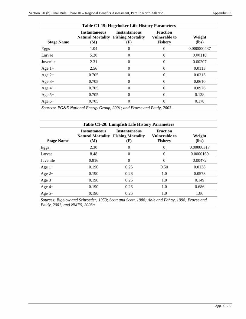
Section 316(b) Final Rule: Phase III – Regional Benefits Assessment, Part C: North Atlantic Appendix C1
App. C1-11
Table C1-19: Hogchoker Life History Parameters
Stage Name
Instantaneous Natural Mortality
(M)
Instantaneous Fishing Mortality
(F)
Fraction Vulnerable to
Fishery Weight
(lbs) Eggs 1.04 0 0 0.000000487 Larvae 5.20 0 0 0.00110 Juvenile 2.31 0 0 0.00207 Age 1+ 2.56 0 0 0.0113 Age 2+ 0.705 0 0 0.0313 Age 3+ 0.705 0 0 0.0610 Age 4+ 0.705 0 0 0.0976 Age 5+ 0.705 0 0 0.138 Age 6+ 0.705 0 0 0.178 Sources: TPG&E National Energy Group, 2001; and Froese and Pauly, 2003T.
Table C1-20: Lumpfish Life History Parameters
Stage Name
Instantaneous Natural Mortality
(M)
Instantaneous Fishing Mortality
(F)
Fraction Vulnerable to
Fishery Weight
(lbs) Eggs 2.30 0 0 0.00000317 Larvae 8.48 0 0 0.0000169 Juvenile 0.916 0 0 0.00472 Age 1+ 0.190 0.26 0.50 0.0138 Age 2+ 0.190 0.26 1.0 0.0573 Age 3+ 0.190 0.26 1.0 0.149 Age 4+ 0.190 0.26 1.0 0.686 Age 5+ 0.190 0.26 1.0 1.86 Sources: Bigelow and Schroeder, 1953; Scott and Scott, 1988; Able and Fahay, 1998; Froese and Pauly, 2001; and NMFS, 2003a.
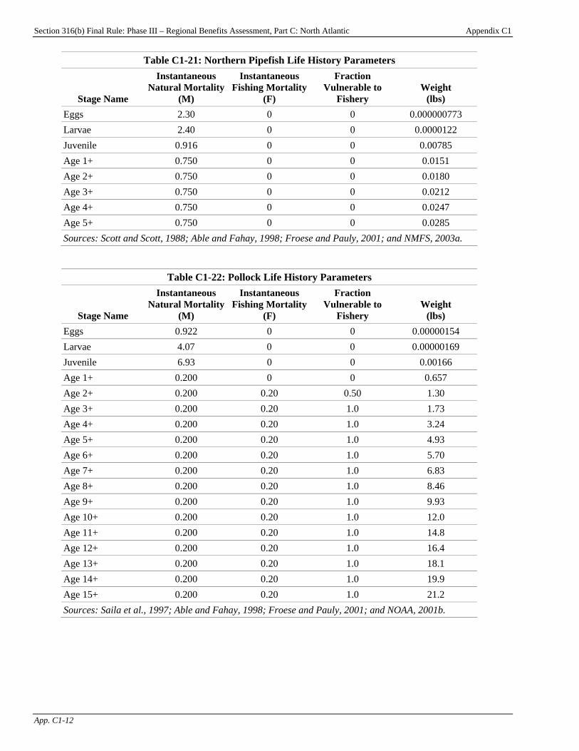
Section 316(b) Final Rule: Phase III – Regional Benefits Assessment, Part C: North Atlantic Appendix C1
App. C1-12
Table C1-21: Northern Pipefish Life History Parameters
Stage Name
Instantaneous Natural Mortality
(M)
Instantaneous Fishing Mortality
(F)
Fraction Vulnerable to
Fishery Weight
(lbs) Eggs 2.30 0 0 0.000000773 Larvae 2.40 0 0 0.0000122 Juvenile 0.916 0 0 0.00785 Age 1+ 0.750 0 0 0.0151 Age 2+ 0.750 0 0 0.0180 Age 3+ 0.750 0 0 0.0212 Age 4+ 0.750 0 0 0.0247 Age 5+ 0.750 0 0 0.0285 Sources: Scott and Scott, 1988; Able and Fahay, 1998; Froese and Pauly, 2001; and NMFS, 2003a.
Table C1-22: Pollock Life History Parameters
Stage Name
Instantaneous Natural Mortality
(M)
Instantaneous Fishing Mortality
(F)
Fraction Vulnerable to
Fishery Weight
(lbs) Eggs 0.922 0 0 0.00000154 Larvae 4.07 0 0 0.00000169 Juvenile 6.93 0 0 0.00166 Age 1+ 0.200 0 0 0.657 Age 2+ 0.200 0.20 0.50 1.30 Age 3+ 0.200 0.20 1.0 1.73 Age 4+ 0.200 0.20 1.0 3.24 Age 5+ 0.200 0.20 1.0 4.93 Age 6+ 0.200 0.20 1.0 5.70 Age 7+ 0.200 0.20 1.0 6.83 Age 8+ 0.200 0.20 1.0 8.46 Age 9+ 0.200 0.20 1.0 9.93 Age 10+ 0.200 0.20 1.0 12.0 Age 11+ 0.200 0.20 1.0 14.8 Age 12+ 0.200 0.20 1.0 16.4 Age 13+ 0.200 0.20 1.0 18.1 Age 14+ 0.200 0.20 1.0 19.9 Age 15+ 0.200 0.20 1.0 21.2 Sources: Saila et al., 1997; Able and Fahay, 1998; Froese and Pauly, 2001; and NOAA, 2001b.
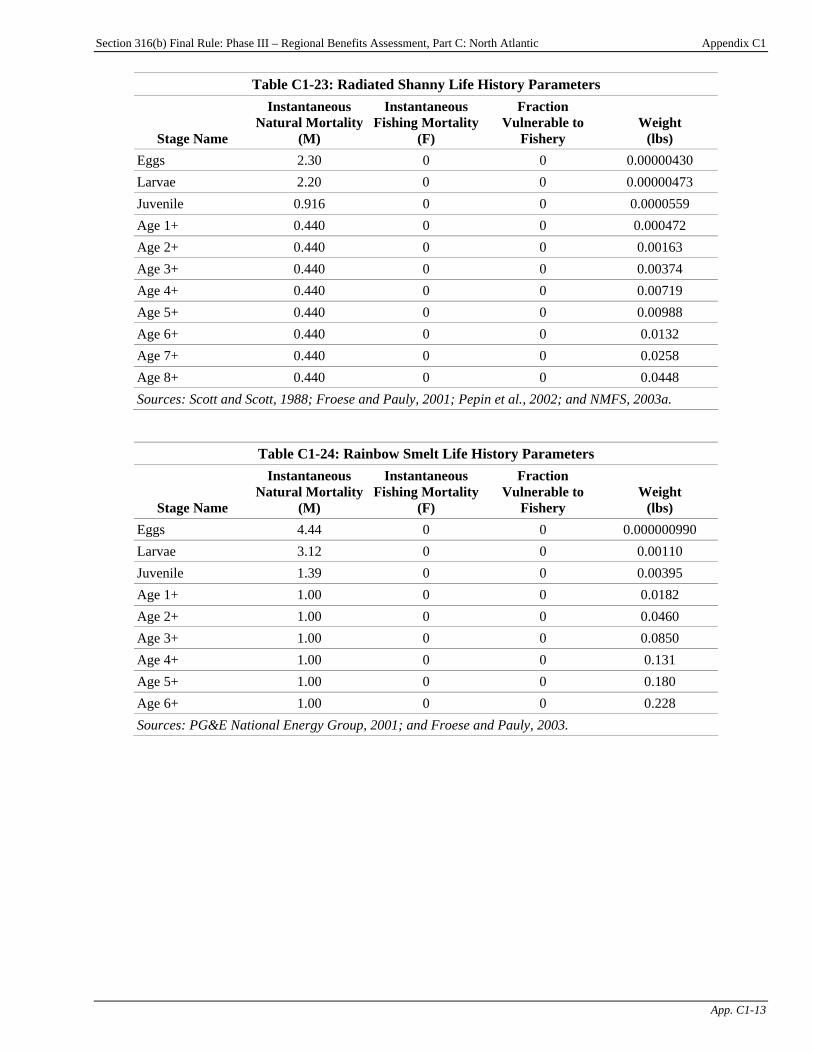
Section 316(b) Final Rule: Phase III – Regional Benefits Assessment, Part C: North Atlantic Appendix C1
App. C1-13
Table C1-23: Radiated Shanny Life History Parameters
Stage Name
Instantaneous Natural Mortality
(M)
Instantaneous Fishing Mortality
(F)
Fraction Vulnerable to
Fishery Weight
(lbs) Eggs 2.30 0 0 0.00000430 Larvae 2.20 0 0 0.00000473 Juvenile 0.916 0 0 0.0000559 Age 1+ 0.440 0 0 0.000472 Age 2+ 0.440 0 0 0.00163 Age 3+ 0.440 0 0 0.00374 Age 4+ 0.440 0 0 0.00719 Age 5+ 0.440 0 0 0.00988 Age 6+ 0.440 0 0 0.0132 Age 7+ 0.440 0 0 0.0258 Age 8+ 0.440 0 0 0.0448 Sources: Scott and Scott, 1988; Froese and Pauly, 2001; Pepin et al., 2002; and NMFS, 2003a.
Table C1-24: Rainbow Smelt Life History Parameters
Stage Name
Instantaneous Natural Mortality
(M)
Instantaneous Fishing Mortality
(F)
Fraction Vulnerable to
Fishery Weight
(lbs) Eggs 4.44 0 0 0.000000990 Larvae 3.12 0 0 0.00110 Juvenile 1.39 0 0 0.00395 Age 1+ 1.00 0 0 0.0182 Age 2+ 1.00 0 0 0.0460 Age 3+ 1.00 0 0 0.0850 Age 4+ 1.00 0 0 0.131 Age 5+ 1.00 0 0 0.180 Age 6+ 1.00 0 0 0.228 Sources: PG&E National Energy Group, 2001; and Froese and Pauly, 2003.
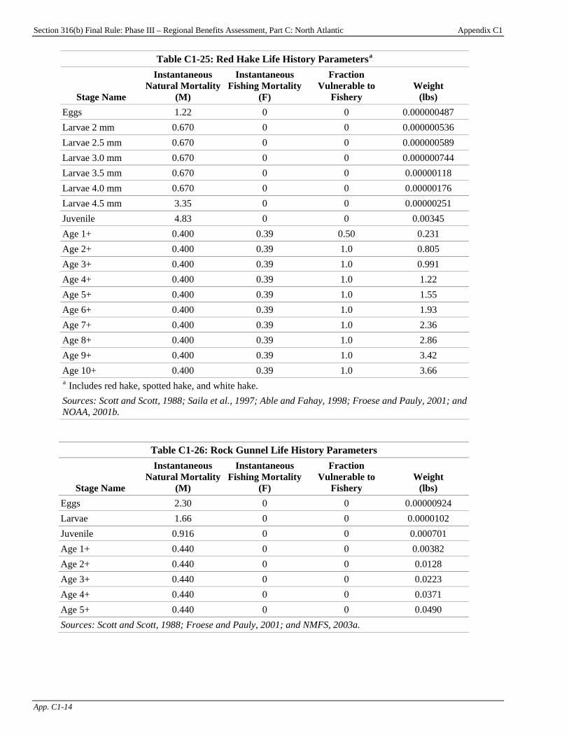
Section 316(b) Final Rule: Phase III – Regional Benefits Assessment, Part C: North Atlantic Appendix C1
App. C1-14
Table C1-25: Red Hake Life History ParametersP
aP
Stage Name
Instantaneous Natural Mortality
(M)
Instantaneous Fishing Mortality
(F)
Fraction Vulnerable to
Fishery Weight
(lbs) Eggs 1.22 0 0 0.000000487 Larvae 2 mm 0.670 0 0 0.000000536 Larvae 2.5 mm 0.670 0 0 0.000000589 Larvae 3.0 mm 0.670 0 0 0.000000744 Larvae 3.5 mm 0.670 0 0 0.00000118 Larvae 4.0 mm 0.670 0 0 0.00000176 Larvae 4.5 mm 3.35 0 0 0.00000251 Juvenile 4.83 0 0 0.00345 Age 1+ 0.400 0.39 0.50 0.231 Age 2+ 0.400 0.39 1.0 0.805 Age 3+ 0.400 0.39 1.0 0.991 Age 4+ 0.400 0.39 1.0 1.22 Age 5+ 0.400 0.39 1.0 1.55 Age 6+ 0.400 0.39 1.0 1.93 Age 7+ 0.400 0.39 1.0 2.36 Age 8+ 0.400 0.39 1.0 2.86 Age 9+ 0.400 0.39 1.0 3.42 Age 10+ 0.400 0.39 1.0 3.66 P
aP Includes red hake, spotted hake, and white hake.
Sources: Scott and Scott, 1988; Saila et al., 1997; Able and Fahay, 1998; Froese and Pauly, 2001; and NOAA, 2001b.
Table C1-26: Rock Gunnel Life History Parameters
Stage Name
Instantaneous Natural Mortality
(M)
Instantaneous Fishing Mortality
(F)
Fraction Vulnerable to
Fishery Weight
(lbs) Eggs 2.30 0 0 0.00000924 Larvae 1.66 0 0 0.0000102 Juvenile 0.916 0 0 0.000701 Age 1+ 0.440 0 0 0.00382 Age 2+ 0.440 0 0 0.0128 Age 3+ 0.440 0 0 0.0223 Age 4+ 0.440 0 0 0.0371 Age 5+ 0.440 0 0 0.0490 Sources: Scott and Scott, 1988; Froese and Pauly, 2001; and NMFS, 2003a.

Section 316(b) Final Rule: Phase III – Regional Benefits Assessment, Part C: North Atlantic Appendix C1
App. C1-15
Table C1-27: Sculpin Life History ParametersP
aP
Stage Name
Instantaneous Natural Mortality
(M)
Instantaneous Fishing Mortality
(F)
Fraction Vulnerable to
Fishery Weight
(lbs) Eggs 2.30 0 0 0.0000107 Larvae 3.79 0 0 0.0000118 Juvenile 0.916 0 0 0.000754 Age 1+ 0.460 0.50 0.50 0.00404 Age 2+ 0.460 0.50 1.0 0.139 Age 3+ 0.460 0.50 1.0 0.332 Age 4+ 0.460 0.50 1.0 0.420 Age 5+ 0.460 0.50 1.0 0.475 Age 6+ 0.460 0.50 1.0 0.541 Age 7+ 0.460 0.50 1.0 0.576 Age 8+ 0.460 0.50 1.0 0.612 Age 9+ 0.460 0.50 1.0 0.637 P
aP Includes longhorn sculpin, moustache sculpin, shorthorn sculpin, and other sculpin not identified to
species. Sources: Clayton et al., 1978; Scott and Scott, 1988; Froese and Pauly, 2001; and personal communication with Y. DeReynier (NMFS, November 19, 2002).
Table C1-28: Scup Life History Parameters
Stage Name
Instantaneous Natural Mortality
(M)
Instantaneous Fishing Mortality
(F)
Fraction Vulnerable to
Fishery Weight
(lbs) Eggs 1.43 0 0 0.000000773 Larvae 4.55 0 0 0.00110 Juvenile 3.36 0 0 0.0280 Age 1+ 0.383 0 0 0.132 Age 2+ 0.383 0 0 0.322 Age 3+ 0.383 0.26 1.0 0.572 Age 4+ 0.383 0.26 1.0 0.845 Age 5+ 0.383 0.26 1.0 1.12 Age 6+ 0.383 0.26 1.0 1.37 Age 7+ 0.383 0.26 1.0 1.59 Age 8+ 0.383 0.26 1.0 1.78 Age 9+ 0.383 0.26 1.0 1.94 Age 10+ 0.383 0.26 1.0 2.07 Age 11+ 0.383 0.26 1.0 2.23 Sources: TPG&E National Energy Group, 2001; and Froese and Pauly, 2003T.
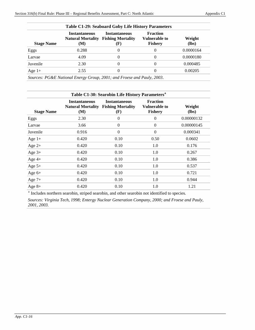
Section 316(b) Final Rule: Phase III – Regional Benefits Assessment, Part C: North Atlantic Appendix C1
App. C1-16
Table C1-29: Seaboard Goby Life History Parameters
Stage Name
Instantaneous Natural Mortality
(M)
Instantaneous Fishing Mortality
(F)
Fraction Vulnerable to
Fishery Weight
(lbs) Eggs 0.288 0 0 0.0000164 Larvae 4.09 0 0 0.0000180 Juvenile 2.30 0 0 0.000485 Age 1+ 2.55 0 0 0.00205 Sources: TPG&E National Energy Group, 2001; and Froese and Pauly, 2003T.
Table C1-30: Searobin Life History ParametersP
aP
Stage Name
Instantaneous Natural Mortality
(M)
Instantaneous Fishing Mortality
(F)
Fraction Vulnerable to
Fishery Weight
(lbs) Eggs 2.30 0 0 0.00000132 Larvae 3.66 0 0 0.00000145 Juvenile 0.916 0 0 0.000341 Age 1+ 0.420 0.10 0.50 0.0602 Age 2+ 0.420 0.10 1.0 0.176 Age 3+ 0.420 0.10 1.0 0.267 Age 4+ 0.420 0.10 1.0 0.386 Age 5+ 0.420 0.10 1.0 0.537 Age 6+ 0.420 0.10 1.0 0.721 Age 7+ 0.420 0.10 1.0 0.944 Age 8+ 0.420 0.10 1.0 1.21 P
aP Includes northern searobin, striped searobin, and other searobin not identified to species.
Sources: Virginia Tech, 1998; Entergy Nuclear Generation Company, 2000; and Froese and Pauly, 2001, 2003.

Section 316(b) Final Rule: Phase III – Regional Benefits Assessment, Part C: North Atlantic Appendix C1
App. C1-17
Table C1-31: Silver Hake Life History Parameters
Stage Name
Instantaneous Natural Mortality
(M)
Instantaneous Fishing Mortality
(F)
Fraction Vulnerable to
Fishery Weight
(lbs) Eggs 1.43 0 0 0.0000203 Larvae 6.62 0 0 0.0000223 Juvenile 4.58 0 0 0.00516 Age 1+ 0.400 0 0 0.0729 Age 2+ 0.400 0 0 0.242 Age 3+ 0.400 0.40 1.0 0.456 Age 4+ 0.400 0.40 1.0 0.646 Age 5+ 0.400 0.40 1.0 0.788 Age 6+ 0.400 0.40 1.0 0.889 Age 7+ 0.400 0.40 1.0 0.958 Age 8+ 0.400 0.40 1.0 1.00 Age 9+ 0.400 0.40 1.0 1.03 Age 10+ 0.400 0.40 1.0 1.05 Age 11+ 0.400 0.40 1.0 1.06 Age 12+ 0.400 0.40 1.0 1.06 Source: PG&E National Energy Group, 2001.
Table C1-32: Skate Species Life History ParametersP
aP
Stage Name
Instantaneous Natural Mortality
(M)
Instantaneous Fishing Mortality
(F)
Fraction Vulnerable to
Fishery Weight
(lbs) Eggs 3.00 0 0 0.0125 Larvae 2.30 0 0 0.0138 Juvenile 0.916 0 0 0.0593 Age 1+ 0.400 0.40 0.50 0.157 Age 2+ 0.400 0.40 1.0 0.394 Age 3+ 0.400 0.40 1.0 0.750 Age 4+ 0.400 0.40 1.0 1.15 Age 5+ 0.400 0.40 1.0 1.51 Age 6+ 0.400 0.40 1.0 1.62 Age 7+ 0.400 0.40 1.0 1.65 Age 8+ 0.400 0.40 1.0 1.72 P
aP Includes clearnose skate, little skate, and other skates not identified to species.
Sources: Scott and Scott, 1988; NOAA, 1993, 2001b; and Froese and Pauly, 2000.

Section 316(b) Final Rule: Phase III – Regional Benefits Assessment, Part C: North Atlantic Appendix C1
App. C1-18
Table C1-33: Striped Bass Life History Parameters
Stage Name
Instantaneous Natural Mortality
(M)
Instantaneous Fishing Mortality
(F)
Fraction Vulnerable to
Fishery Weight
(lbs) Eggs 2.28 0 0 0.0000282 Larvae 6.28 0 0 0.0000310 Juvenile 5.63 0 0 0.0405 Age 1+ 1.11 0 0 0.386 Age 2+ 0.150 0.02 1.0 1.37 Age 3+ 0.150 0.06 1.0 3.06 Age 4+ 0.150 0.20 1.0 5.35 Age 5+ 0.150 0.29 1.0 8.07 Age 6+ 0.150 0.31 1.0 11.0 Age 7+ 0.150 0.31 1.0 14.1 Age 8+ 0.150 0.31 1.0 17.1 Age 9+ 0.150 0.31 1.0 20.0 Age 10+ 0.150 0.31 1.0 22.8 Age 11+ 0.150 0.31 1.0 25.3 Age 12+ 0.150 0.31 1.0 27.6 Age 13+ 0.150 0.31 1.0 29.7 Age 14+ 0.150 0.31 1.0 31.6 Age 15+ 0.150 0.31 1.0 33.3 Age 16+ 0.150 0.31 1.0 34.7 Age 17+ 0.150 0.31 1.0 36.0 Age 18+ 0.150 0.31 1.0 37.2 Age 19+ 0.150 0.31 1.0 38.2 Age 20+ 0.150 0.31 1.0 39.0 Age 21+ 0.150 0.31 1.0 39.8 Age 22+ 0.150 0.31 1.0 40.4 Age 23+ 0.150 0.31 1.0 41.0 Age 24+ 0.150 0.31 1.0 41.5 Source: PG&E National Energy Group, 2001.
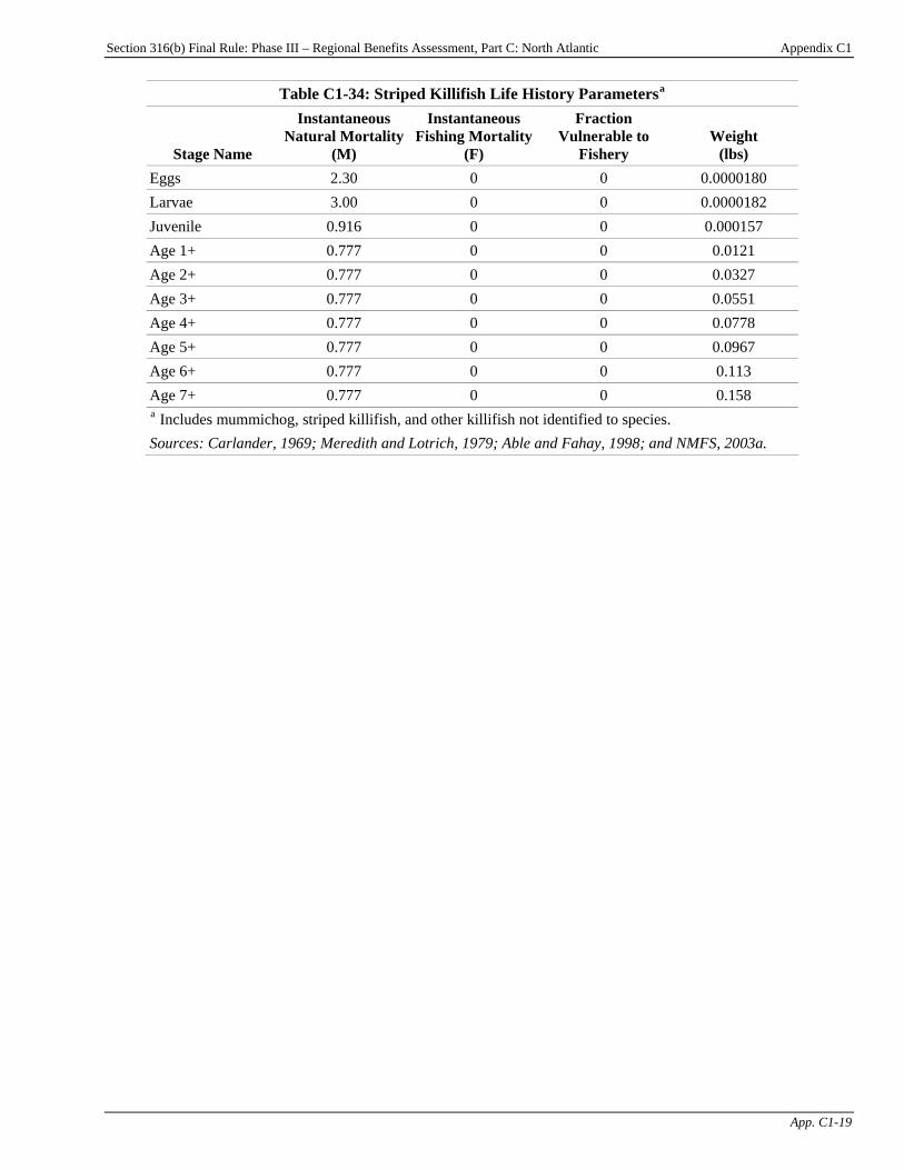
Section 316(b) Final Rule: Phase III – Regional Benefits Assessment, Part C: North Atlantic Appendix C1
App. C1-19
Table C1-34: Striped Killifish Life History ParametersP
aP
Stage Name
Instantaneous Natural Mortality
(M)
Instantaneous Fishing Mortality
(F)
Fraction Vulnerable to
Fishery Weight
(lbs) Eggs 2.30 0 0 0.0000180 Larvae 3.00 0 0 0.0000182 Juvenile 0.916 0 0 0.000157 Age 1+ 0.777 0 0 0.0121 Age 2+ 0.777 0 0 0.0327 Age 3+ 0.777 0 0 0.0551 Age 4+ 0.777 0 0 0.0778 Age 5+ 0.777 0 0 0.0967 Age 6+ 0.777 0 0 0.113 Age 7+ 0.777 0 0 0.158 P
aP Includes mummichog, striped killifish, and other killifish not identified to species.
Sources: Carlander, 1969; Meredith and Lotrich, 1979; Able and Fahay, 1998; and NMFS, 2003a.
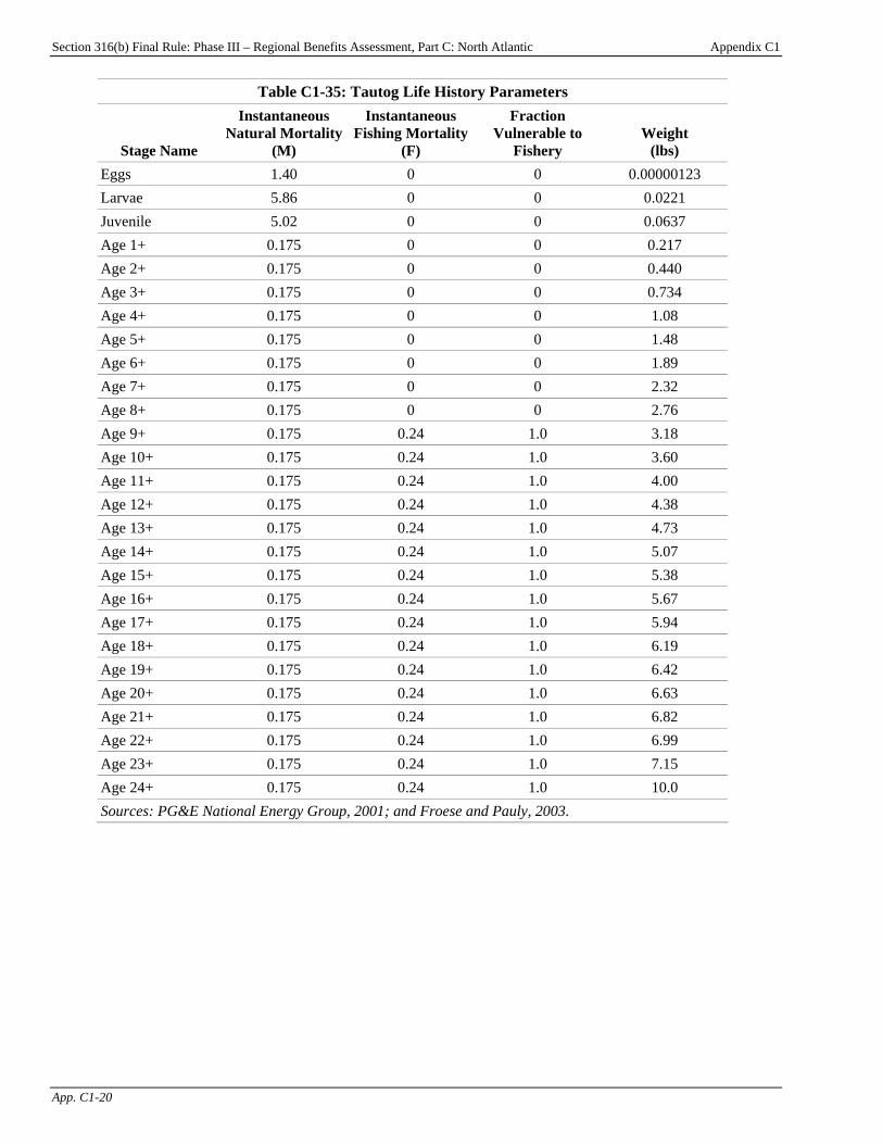
Section 316(b) Final Rule: Phase III – Regional Benefits Assessment, Part C: North Atlantic Appendix C1
App. C1-20
Table C1-35: Tautog Life History Parameters
Stage Name
Instantaneous Natural Mortality
(M)
Instantaneous Fishing Mortality
(F)
Fraction Vulnerable to
Fishery Weight
(lbs) Eggs 1.40 0 0 0.00000123 Larvae 5.86 0 0 0.0221 Juvenile 5.02 0 0 0.0637 Age 1+ 0.175 0 0 0.217 Age 2+ 0.175 0 0 0.440 Age 3+ 0.175 0 0 0.734 Age 4+ 0.175 0 0 1.08 Age 5+ 0.175 0 0 1.48 Age 6+ 0.175 0 0 1.89 Age 7+ 0.175 0 0 2.32 Age 8+ 0.175 0 0 2.76 Age 9+ 0.175 0.24 1.0 3.18 Age 10+ 0.175 0.24 1.0 3.60 Age 11+ 0.175 0.24 1.0 4.00 Age 12+ 0.175 0.24 1.0 4.38 Age 13+ 0.175 0.24 1.0 4.73 Age 14+ 0.175 0.24 1.0 5.07 Age 15+ 0.175 0.24 1.0 5.38 Age 16+ 0.175 0.24 1.0 5.67 Age 17+ 0.175 0.24 1.0 5.94 Age 18+ 0.175 0.24 1.0 6.19 Age 19+ 0.175 0.24 1.0 6.42 Age 20+ 0.175 0.24 1.0 6.63 Age 21+ 0.175 0.24 1.0 6.82 Age 22+ 0.175 0.24 1.0 6.99 Age 23+ 0.175 0.24 1.0 7.15 Age 24+ 0.175 0.24 1.0 10.0 Sources: PG&E National Energy Group, 2001; and Froese and Pauly, 2003.
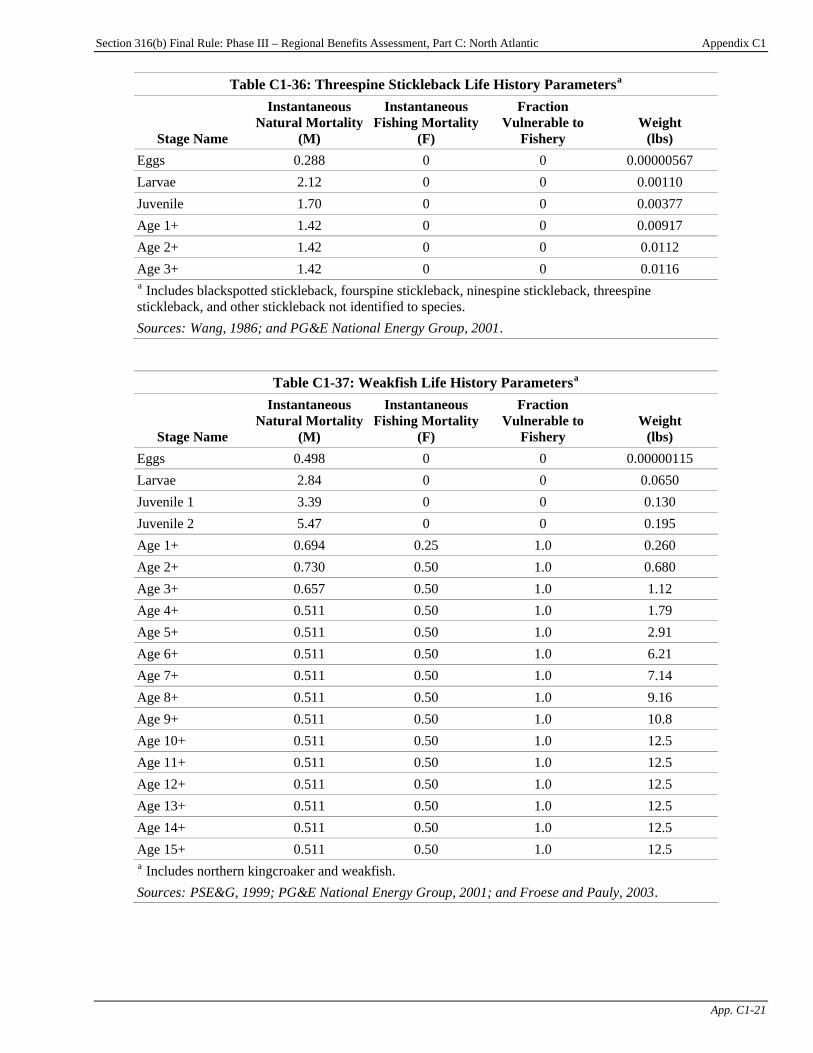
Section 316(b) Final Rule: Phase III – Regional Benefits Assessment, Part C: North Atlantic Appendix C1
App. C1-21
Table C1-36: Threespine Stickleback Life History ParametersP
aP
Stage Name
Instantaneous Natural Mortality
(M)
Instantaneous Fishing Mortality
(F)
Fraction Vulnerable to
Fishery Weight
(lbs) Eggs 0.288 0 0 0.00000567 Larvae 2.12 0 0 0.00110 Juvenile 1.70 0 0 0.00377 Age 1+ 1.42 0 0 0.00917 Age 2+ 1.42 0 0 0.0112 Age 3+ 1.42 0 0 0.0116 P
aP Includes blackspotted stickleback, fourspine stickleback, ninespine stickleback, threespine
stickleback, and other stickleback not identified to species. Sources:T Wang, 1986; and PG&E National Energy Group, 2001T.
Table C1-37: Weakfish Life History ParametersP
aP
Stage Name
Instantaneous Natural Mortality
(M)
Instantaneous Fishing Mortality
(F)
Fraction Vulnerable to
Fishery Weight
(lbs) Eggs 0.498 0 0 0.00000115 Larvae 2.84 0 0 0.0650 Juvenile 1 3.39 0 0 0.130 Juvenile 2 5.47 0 0 0.195 Age 1+ 0.694 0.25 1.0 0.260 Age 2+ 0.730 0.50 1.0 0.680 Age 3+ 0.657 0.50 1.0 1.12 Age 4+ 0.511 0.50 1.0 1.79 Age 5+ 0.511 0.50 1.0 2.91 Age 6+ 0.511 0.50 1.0 6.21 Age 7+ 0.511 0.50 1.0 7.14 Age 8+ 0.511 0.50 1.0 9.16 Age 9+ 0.511 0.50 1.0 10.8 Age 10+ 0.511 0.50 1.0 12.5 Age 11+ 0.511 0.50 1.0 12.5 Age 12+ 0.511 0.50 1.0 12.5 Age 13+ 0.511 0.50 1.0 12.5 Age 14+ 0.511 0.50 1.0 12.5 Age 15+ 0.511 0.50 1.0 12.5 P
aP Includes northern kingcroaker and weakfish.
Sources:T PSE&G, 1999; PG&E National Energy Group, 2001; and Froese and Pauly, 2003T.
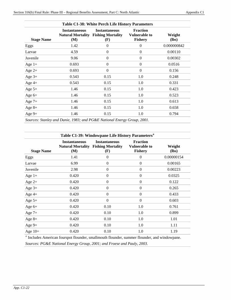
Section 316(b) Final Rule: Phase III – Regional Benefits Assessment, Part C: North Atlantic Appendix C1
App. C1-22
Table C1-38: White Perch Life History Parameters
Stage Name
Instantaneous Natural Mortality
(M)
Instantaneous Fishing Mortality
(F)
Fraction Vulnerable to
Fishery Weight
(lbs) Eggs 1.42 0 0 0.000000842 Larvae 4.59 0 0 0.00110 Juvenile 9.06 0 0 0.00302 Age 1+ 0.693 0 0 0.0516 Age 2+ 0.693 0 0 0.156 Age 3+ 0.543 0.15 1.0 0.248 Age 4+ 0.543 0.15 1.0 0.331 Age 5+ 1.46 0.15 1.0 0.423 Age 6+ 1.46 0.15 1.0 0.523 Age 7+ 1.46 0.15 1.0 0.613 Age 8+ 1.46 0.15 1.0 0.658 Age 9+ 1.46 0.15 1.0 0.794 Sources: Stanley and Danie, 1983; and PG&E National Energy Group, 2001.
Table C1-39: Windowpane Life History ParametersP
aP
Stage Name
Instantaneous Natural Mortality
(M)
Instantaneous Fishing Mortality
(F)
Fraction Vulnerable to
Fishery Weight
(lbs) Eggs 1.41 0 0 0.00000154 Larvae 6.99 0 0 0.00165 Juvenile 2.98 0 0 0.00223 Age 1+ 0.420 0 0 0.0325 Age 2+ 0.420 0 0 0.122 Age 3+ 0.420 0 0 0.265 Age 4+ 0.420 0 0 0.433 Age 5+ 0.420 0 0 0.603 Age 6+ 0.420 0.10 1.0 0.761 Age 7+ 0.420 0.10 1.0 0.899 Age 8+ 0.420 0.10 1.0 1.01 Age 9+ 0.420 0.10 1.0 1.11 Age 10+ 0.420 0.10 1.0 1.19 P
aP Includes American fourspot flounder, smallmouth flounder, summer flounder, and windowpane.
Sources: PG&E National Energy Group, 2001; and Froese and Pauly, 2003.
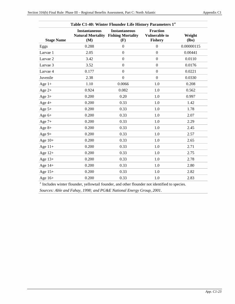
Section 316(b) Final Rule: Phase III – Regional Benefits Assessment, Part C: North Atlantic Appendix C1
App. C1-23
Table C1-40: Winter Flounder Life History Parameters 1P
aP
Stage Name
Instantaneous Natural Mortality
(M)
Instantaneous Fishing Mortality
(F)
Fraction Vulnerable to
Fishery Weight
(lbs) Eggs 0.288 0 0 0.00000115 Larvae 1 2.05 0 0 0.00441 Larvae 2 3.42 0 0 0.0110 Larvae 3 3.52 0 0 0.0176 Larvae 4 0.177 0 0 0.0221 Juvenile 2.38 0 0 0.0330 Age 1+ 1.10 0.0066 1.0 0.208 Age 2+ 0.924 0.082 1.0 0.562 Age 3+ 0.200 0.20 1.0 0.997 Age 4+ 0.200 0.33 1.0 1.42 Age 5+ 0.200 0.33 1.0 1.78 Age 6+ 0.200 0.33 1.0 2.07 Age 7+ 0.200 0.33 1.0 2.29 Age 8+ 0.200 0.33 1.0 2.45 Age 9+ 0.200 0.33 1.0 2.57 Age 10+ 0.200 0.33 1.0 2.65 Age 11+ 0.200 0.33 1.0 2.71 Age 12+ 0.200 0.33 1.0 2.75 Age 13+ 0.200 0.33 1.0 2.78 Age 14+ 0.200 0.33 1.0 2.80 Age 15+ 0.200 0.33 1.0 2.82 Age 16+ 0.200 0.33 1.0 2.83 P
aP Includes winter flounder, yellowtail founder, and other flounder not identified to species.
Sources: Able and Fahay, 1998; Tand PG&E National Energy Group, 2001T.
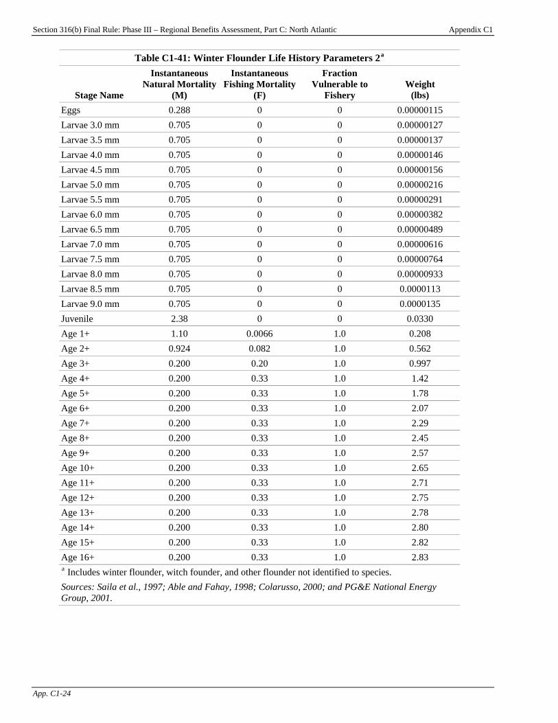
Section 316(b) Final Rule: Phase III – Regional Benefits Assessment, Part C: North Atlantic Appendix C1
App. C1-24
Table C1-41: Winter Flounder Life History Parameters 2P
aP
Stage Name
Instantaneous Natural Mortality
(M)
Instantaneous Fishing Mortality
(F)
Fraction Vulnerable to
Fishery Weight
(lbs) Eggs 0.288 0 0 0.00000115 Larvae 3.0 mm 0.705 0 0 0.00000127 Larvae 3.5 mm 0.705 0 0 0.00000137 Larvae 4.0 mm 0.705 0 0 0.00000146 Larvae 4.5 mm 0.705 0 0 0.00000156 Larvae 5.0 mm 0.705 0 0 0.00000216 Larvae 5.5 mm 0.705 0 0 0.00000291 Larvae 6.0 mm 0.705 0 0 0.00000382 Larvae 6.5 mm 0.705 0 0 0.00000489 Larvae 7.0 mm 0.705 0 0 0.00000616 Larvae 7.5 mm 0.705 0 0 0.00000764 Larvae 8.0 mm 0.705 0 0 0.00000933 Larvae 8.5 mm 0.705 0 0 0.0000113 Larvae 9.0 mm 0.705 0 0 0.0000135 Juvenile 2.38 0 0 0.0330 Age 1+ 1.10 0.0066 1.0 0.208 Age 2+ 0.924 0.082 1.0 0.562 Age 3+ 0.200 0.20 1.0 0.997 Age 4+ 0.200 0.33 1.0 1.42 Age 5+ 0.200 0.33 1.0 1.78 Age 6+ 0.200 0.33 1.0 2.07 Age 7+ 0.200 0.33 1.0 2.29 Age 8+ 0.200 0.33 1.0 2.45 Age 9+ 0.200 0.33 1.0 2.57 Age 10+ 0.200 0.33 1.0 2.65 Age 11+ 0.200 0.33 1.0 2.71 Age 12+ 0.200 0.33 1.0 2.75 Age 13+ 0.200 0.33 1.0 2.78 Age 14+ 0.200 0.33 1.0 2.80 Age 15+ 0.200 0.33 1.0 2.82 Age 16+ 0.200 0.33 1.0 2.83 P
aP Includes winter flounder, witch founder, and other flounder not identified to species.
Sources: Saila et al., 1997; Able and Fahay, 1998; Colarusso, 2000; and PG&E National Energy Group, 2001.
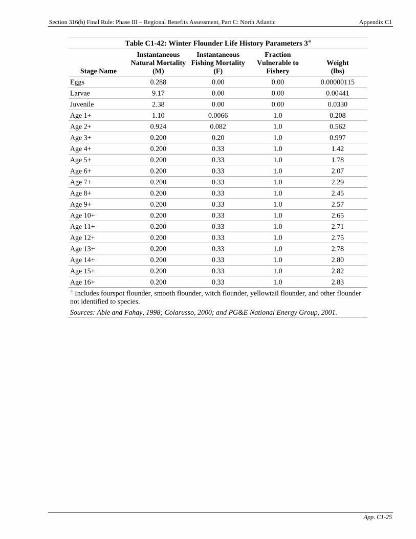
Section 316(b) Final Rule: Phase III – Regional Benefits Assessment, Part C: North Atlantic Appendix C1
App. C1-25
Table C1-42: Winter Flounder Life History Parameters 3P
aP
Stage Name
Instantaneous Natural Mortality
(M)
Instantaneous Fishing Mortality
(F)
Fraction Vulnerable to
Fishery Weight
(lbs) Eggs 0.288 0.00 0.00 0.00000115 Larvae 9.17 0.00 0.00 0.00441 Juvenile 2.38 0.00 0.00 0.0330 Age 1+ 1.10 0.0066 1.0 0.208 Age 2+ 0.924 0.082 1.0 0.562 Age 3+ 0.200 0.20 1.0 0.997 Age 4+ 0.200 0.33 1.0 1.42 Age 5+ 0.200 0.33 1.0 1.78 Age 6+ 0.200 0.33 1.0 2.07 Age 7+ 0.200 0.33 1.0 2.29 Age 8+ 0.200 0.33 1.0 2.45 Age 9+ 0.200 0.33 1.0 2.57 Age 10+ 0.200 0.33 1.0 2.65 Age 11+ 0.200 0.33 1.0 2.71 Age 12+ 0.200 0.33 1.0 2.75 Age 13+ 0.200 0.33 1.0 2.78 Age 14+ 0.200 0.33 1.0 2.80 Age 15+ 0.200 0.33 1.0 2.82 Age 16+ 0.200 0.33 1.0 2.83 P
aP Includes fourspot flounder, smooth flounder, witch flounder, yellowtail flounder, and other flounder
not identified to species.
Sources: Able and Fahay, 1998; Colarusso, 2000; and PG&E National Energy Group, 2001.
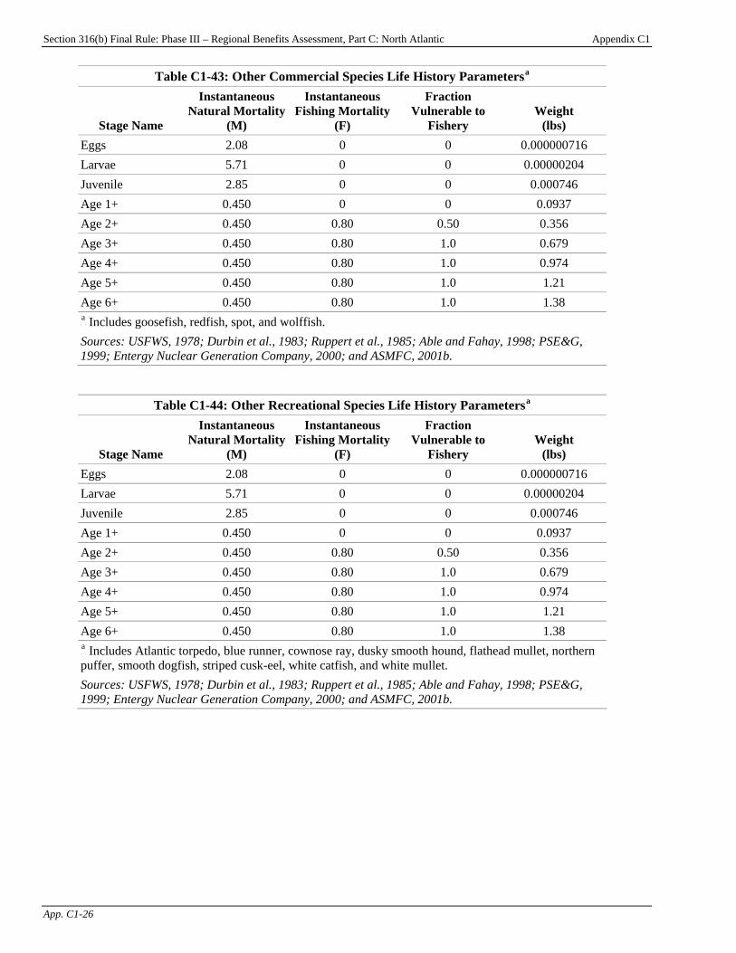
Section 316(b) Final Rule: Phase III – Regional Benefits Assessment, Part C: North Atlantic Appendix C1
App. C1-26
Table C1-43: Other Commercial Species Life History ParametersP
aP
Stage Name
Instantaneous Natural Mortality
(M)
Instantaneous Fishing Mortality
(F)
Fraction Vulnerable to
Fishery Weight
(lbs) Eggs 2.08 0 0 0.000000716 Larvae 5.71 0 0 0.00000204 Juvenile 2.85 0 0 0.000746 Age 1+ 0.450 0 0 0.0937 Age 2+ 0.450 0.80 0.50 0.356 Age 3+ 0.450 0.80 1.0 0.679 Age 4+ 0.450 0.80 1.0 0.974 Age 5+ 0.450 0.80 1.0 1.21 Age 6+ 0.450 0.80 1.0 1.38 P
aP Includes goosefish, redfish, spot, and wolffish.
Sources: USFWS, 1978; Durbin et al., 1983; Ruppert et al., 1985; Able and Fahay, 1998; PSE&G, 1999; Entergy Nuclear Generation Company, 2000; and ASMFC, 2001b.
Table C1-44: Other Recreational Species Life History ParametersP
aP
Stage Name
Instantaneous Natural Mortality
(M)
Instantaneous Fishing Mortality
(F)
Fraction Vulnerable to
Fishery Weight
(lbs) Eggs 2.08 0 0 0.000000716 Larvae 5.71 0 0 0.00000204 Juvenile 2.85 0 0 0.000746 Age 1+ 0.450 0 0 0.0937 Age 2+ 0.450 0.80 0.50 0.356 Age 3+ 0.450 0.80 1.0 0.679 Age 4+ 0.450 0.80 1.0 0.974 Age 5+ 0.450 0.80 1.0 1.21 Age 6+ 0.450 0.80 1.0 1.38 P
aP Includes Atlantic torpedo, blue runner, cownose ray, dusky smooth hound, flathead mullet, northern
puffer, smooth dogfish, striped cusk-eel, white catfish, and white mullet. Sources: USFWS, 1978; Durbin et al., 1983; Ruppert et al., 1985; Able and Fahay, 1998; PSE&G, 1999; Entergy Nuclear Generation Company, 2000; and ASMFC, 2001b.

Section 316(b) Final Rule: Phase III – Regional Benefits Assessment, Part C: North Atlantic Appendix C1
App. C1-27
Table C1-45: Other Recreational and Commercial Species Life History ParametersP
aP
Stage Name
Instantaneous Natural Mortality
(M)
Instantaneous Fishing Mortality
(F)
Fraction Vulnerable to
Fishery Weight
(lbs) Eggs 2.08 0 0 0.000000716 Larvae 5.71 0 0 0.00000204 Juvenile 1 1.43 0 0 0.000746 Juvenile 2 1.43 0 0 0.0472 Age 1+ 0.450 0 0 0.0937 Age 2+ 0.450 0.80 0.50 0.356 Age 3+ 0.450 0.80 1.0 0.679 Age 4+ 0.450 0.80 1.0 0.974 Age 5+ 0.450 0.80 1.0 1.21 Age 6+ 0.450 0.80 1.0 1.38 P
aP Includes American eel, black sea bass, conger eel, and piked dogfish.
Sources: USFWS, 1978; Durbin et al., 1983; Ruppert et al., 1985; Able and Fahay, 1998; PSE&G, 1999; Entergy Nuclear Generation Company, 2000; and ASMFC, 2001b.
Table C1-46: Other Forage Species Life History ParametersP
aP
Stage Name
Instantaneous Natural Mortality
(M)
Instantaneous Fishing Mortality
(F)
Fraction Vulnerable to
Fishery Weight
(lbs) Eggs 1.04 0 0 0.0000000186 Larvae 7.70 0 0 0.00000158 Juvenile 1.29 0 0 0.000480 Age 1+ 1.62 0 0 0.00381 Age 2+ 1.62 0 0 0.00496 Age 3+ 1.62 0 0 0.00505 P
aP See Table C1-47 for a list of species.
Sources: Derickson and Price, 1973; and PSE&G, 1999.
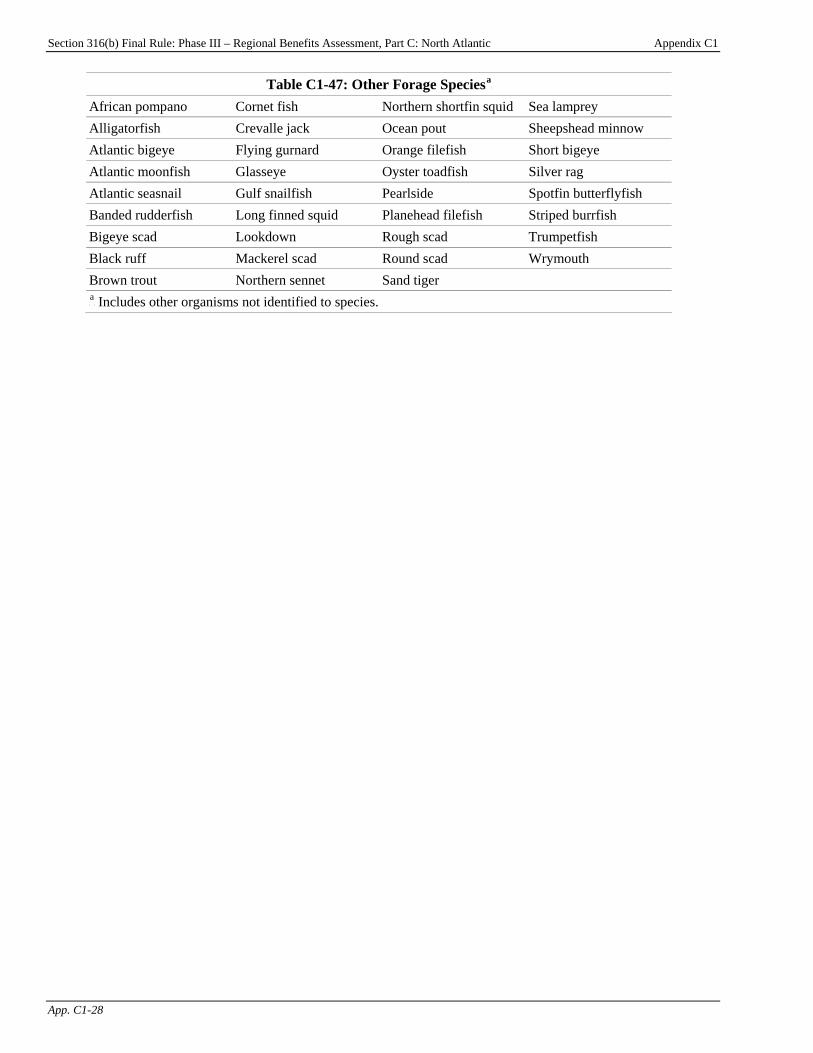
Section 316(b) Final Rule: Phase III – Regional Benefits Assessment, Part C: North Atlantic Appendix C1
App. C1-28
Table C1-47: Other Forage SpeciesP
aP
African pompano Cornet fish Northern shortfin squid Sea lamprey Alligatorfish Crevalle jack Ocean pout Sheepshead minnow Atlantic bigeye Flying gurnard Orange filefish Short bigeye Atlantic moonfish Glasseye Oyster toadfish Silver rag Atlantic seasnail Gulf snailfish Pearlside Spotfin butterflyfish Banded rudderfish Long finned squid Planehead filefish Striped burrfish Bigeye scad Lookdown Rough scad Trumpetfish Black ruff Mackerel scad Round scad Wrymouth Brown trout Northern sennet Sand tiger P
aP Includes other organisms not identified to species.
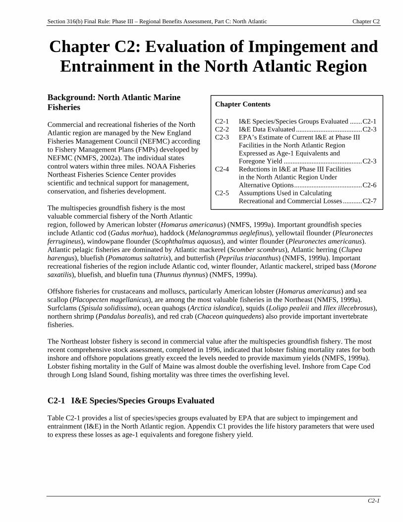
Section 316(b) Final Rule: Phase III – Regional Benefits Assessment, Part C: North Atlantic Chapter C2
C2-1
Chapter C2: Evaluation of Impingement and Entrainment in the North Atlantic Region
Background: North Atlantic Marine Fisheries Commercial and recreational fisheries of the North Atlantic region are managed by the New England Fisheries Management Council (NEFMC) according to Fishery Management Plans (FMPs) developed by NEFMC (NMFS, 2002a). The individual states control waters within three miles. NOAA Fisheries Northeast Fisheries Science Center provides scientific and technical support for management, conservation, and fisheries development. The multispecies groundfish fishery is the most valuable commercial fishery of the North Atlantic region, followed by American lobster (Homarus americanus) (NMFS, 1999a). Important groundfish species include Atlantic cod (Gadus morhua), haddock (Melanogrammus aeglefinus), yellowtail flounder (Pleuronectes ferrugineus), windowpane flounder (Scophthalmus aquosus), and winter flounder (Pleuronectes americanus). Atlantic pelagic fisheries are dominated by Atlantic mackerel (Scomber scombrus), Atlantic herring (Clupea harengus), bluefish (Pomatomus saltatrix), and butterfish (Peprilus triacanthus) (NMFS, 1999a). Important recreational fisheries of the region include Atlantic cod, winter flounder, Atlantic mackerel, striped bass (Morone saxatilis), bluefish, and bluefin tuna (Thunnus thynnus) (NMFS, 1999a).
Chapter Contents C2-1 I&E Species/Species Groups Evaluated .......C2-1 C2-2 I&E Data Evaluated ......................................C2-3 C2-3 EPA’s Estimate of Current I&E at Phase III Facilities in the North Atlantic Region Expressed as Age-1 Equivalents and Foregone Yield .............................................C2-3 C2-4 Reductions in I&E at Phase III Facilities in the North Atlantic Region Under Alternative Options.......................................C2-6 C2-5 Assumptions Used in Calculating Recreational and Commercial Losses ...........C2-7
Offshore fisheries for crustaceans and molluscs, particularly American lobster (Homarus americanus) and sea scallop (Placopecten magellanicus), are among the most valuable fisheries in the Northeast (NMFS, 1999a). Surfclams (Spisula solidissima), ocean quahogs (Arctica islandica), squids (Loligo pealeii and Illex illecebrosus), northern shrimp (Pandalus borealis), and red crab (Chaceon quinquedens) also provide important invertebrate fisheries. The Northeast lobster fishery is second in commercial value after the multispecies groundfish fishery. The most recent comprehensive stock assessment, completed in 1996, indicated that lobster fishing mortality rates for both inshore and offshore populations greatly exceed the levels needed to provide maximum yields (NMFS, 1999a). Lobster fishing mortality in the Gulf of Maine was almost double the overfishing level. Inshore from Cape Cod through Long Island Sound, fishing mortality was three times the overfishing level. C2-1 I&E Species/Species Groups Evaluated Table C2-1 provides a list of species/species groups evaluated by EPA that are subject to impingement and entrainment (I&E) in the North Atlantic region. Appendix C1 provides the life history parameters that were used to express these losses as age-1 equivalents and foregone fishery yield.
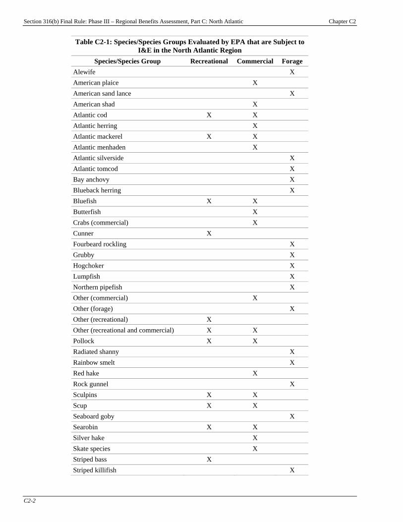
Section 316(b) Final Rule: Phase III – Regional Benefits Assessment, Part C: North Atlantic Chapter C2
C2-2
Table C2-1: Species/Species Groups Evaluated by EPA that are Subject to I&E in the North Atlantic Region
Species/Species Group Recreational Commercial Forage Alewife X American plaice X American sand lance X American shad X Atlantic cod X X Atlantic herring X Atlantic mackerel X X Atlantic menhaden X Atlantic silverside X Atlantic tomcod X Bay anchovy X Blueback herring X Bluefish X X Butterfish X Crabs (commercial) X Cunner X Fourbeard rockling X Grubby X Hogchoker X Lumpfish X Northern pipefish X Other (commercial) X Other (forage) X Other (recreational) X Other (recreational and commercial) X X Pollock X X Radiated shanny X Rainbow smelt X Red hake X Rock gunnel X Sculpins X X Scup X X Seaboard goby X Searobin X X Silver hake X Skate species X Striped bass X Striped killifish X
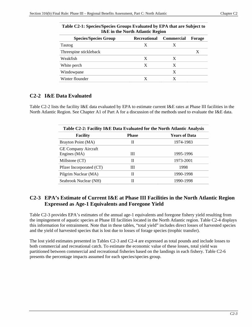
Section 316(b) Final Rule: Phase III – Regional Benefits Assessment, Part C: North Atlantic Chapter C2
C2-3
Table C2-1: Species/Species Groups Evaluated by EPA that are Subject to I&E in the North Atlantic Region
Species/Species Group Recreational Commercial Forage Tautog X X Threespine stickleback X Weakfish X X White perch X X Windowpane X Winter flounder X X
C2-2 I&E Data Evaluated Table C2-2 lists the facility I&E data evaluated by EPA to estimate current I&E rates at Phase III facilities in the North Atlantic Region. See Chapter A1 of Part A for a discussion of the methods used to evaluate the I&E data.
Table C2-2: Facility I&E Data Evaluated for the North Atlantic Analysis Facility Phase Years of Data
Brayton Point (MA) II 1974-1983 GE Company Aircraft Engines (MA) III 1995-1996 Millstone (CT) II 1973-2001 Pfizer Incorporated (CT) III 1998 Pilgrim Nuclear (MA) II 1990-1998 Seabrook Nuclear (NH) II 1990-1998
C2-3 EPA’s Estimate of Current I&E at Phase III Facilities in the North Atlantic Region
Expressed as Age-1 Equivalents and Foregone Yield Table C2-3 provides EPA’s estimates of the annual age-1 equivalents and foregone fishery yield resulting from the impingement of aquatic species at Phase III facilities located in the North Atlantic region. Table C2-4 displays this information for entrainment. Note that in these tables, “total yield” includes direct losses of harvested species and the yield of harvested species that is lost due to losses of forage species (trophic transfer). The lost yield estimates presented in Tables C2-3 and C2-4 are expressed as total pounds and include losses to both commercial and recreational catch. To estimate the economic value of these losses, total yield was partitioned between commercial and recreational fisheries based on the landings in each fishery. Table C2-6 presents the percentage impacts assumed for each species/species group.
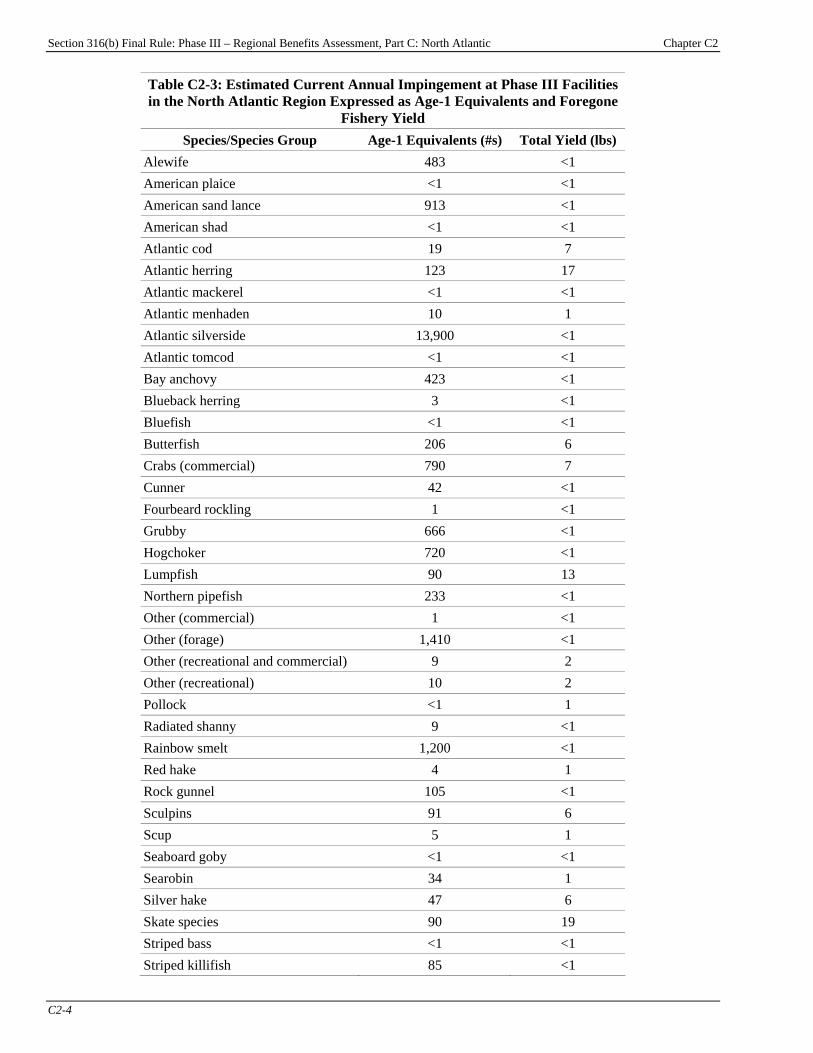
Section 316(b) Final Rule: Phase III – Regional Benefits Assessment, Part C: North Atlantic Chapter C2
C2-4
Table C2-3: Estimated Current Annual Impingement at Phase III Facilities in the North Atlantic Region Expressed as Age-1 Equivalents and Foregone
Fishery Yield Species/Species Group Age-1 Equivalents (#s) Total Yield (lbs)
Alewife 483 <1 American plaice <1 <1 American sand lance 913 <1 American shad <1 <1 Atlantic cod 19 7 Atlantic herring 123 17 Atlantic mackerel <1 <1 Atlantic menhaden 10 1 Atlantic silverside 13,900 <1 Atlantic tomcod <1 <1 Bay anchovy 423 <1 Blueback herring 3 <1 Bluefish <1 <1 Butterfish 206 6 Crabs (commercial) 790 7 Cunner 42 <1 Fourbeard rockling 1 <1 Grubby 666 <1 Hogchoker 720 <1 Lumpfish 90 13 Northern pipefish 233 <1 Other (commercial) 1 <1 Other (forage) 1,410 <1 Other (recreational and commercial) 9 2 Other (recreational) 10 2 Pollock <1 1 Radiated shanny 9 <1 Rainbow smelt 1,200 <1 Red hake 4 1 Rock gunnel 105 <1 Sculpins 91 6 Scup 5 1 Seaboard goby <1 <1 Searobin 34 1 Silver hake 47 6 Skate species 90 19 Striped bass <1 <1 Striped killifish 85 <1
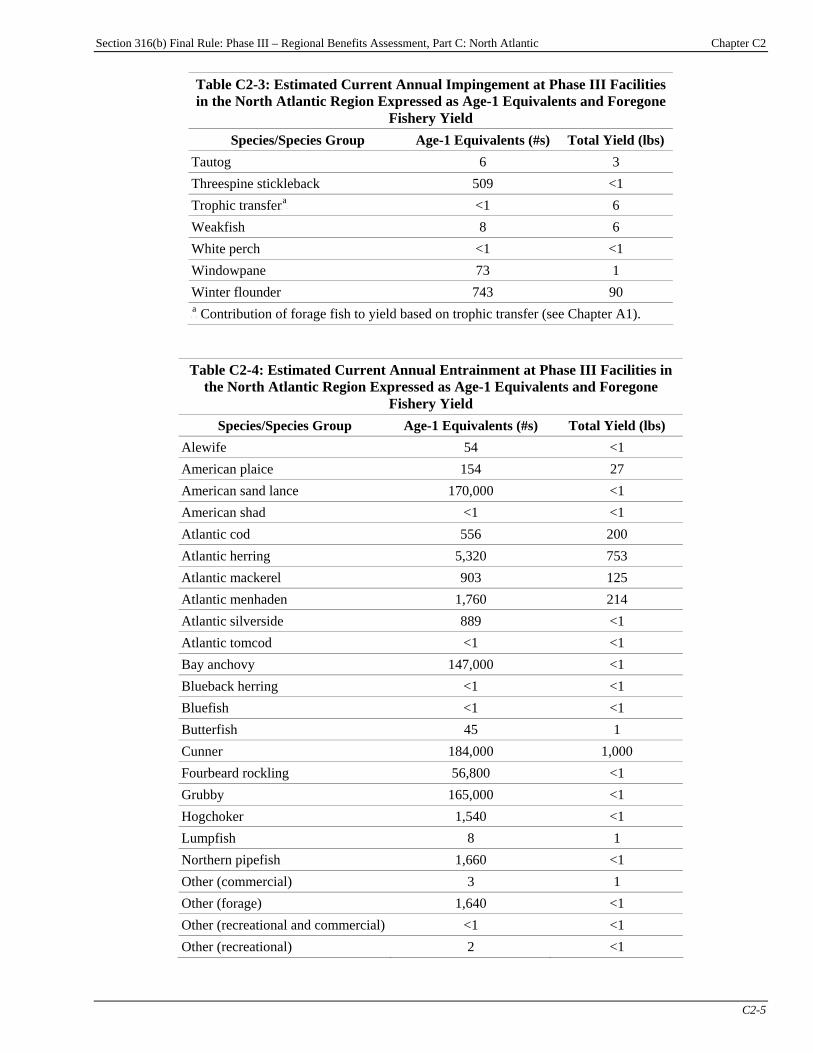
Section 316(b) Final Rule: Phase III – Regional Benefits Assessment, Part C: North Atlantic Chapter C2
C2-5
Table C2-3: Estimated Current Annual Impingement at Phase III Facilities in the North Atlantic Region Expressed as Age-1 Equivalents and Foregone
Fishery Yield Species/Species Group Age-1 Equivalents (#s) Total Yield (lbs)
Tautog 6 3 Threespine stickleback 509 <1 Trophic transferP
aP <1 6
Weakfish 8 6 White perch <1 <1 Windowpane 73 1 Winter flounder 743 90 P
aP Contribution of forage fish to yield based on trophic transfer (see Chapter A1).
Table C2-4: Estimated Current Annual Entrainment at Phase III Facilities in the North Atlantic Region Expressed as Age-1 Equivalents and Foregone
Fishery Yield Species/Species Group Age-1 Equivalents (#s) Total Yield (lbs)
Alewife 54 <1 American plaice 154 27 American sand lance 170,000 <1 American shad <1 <1 Atlantic cod 556 200 Atlantic herring 5,320 753 Atlantic mackerel 903 125 Atlantic menhaden 1,760 214 Atlantic silverside 889 <1 Atlantic tomcod <1 <1 Bay anchovy 147,000 <1 Blueback herring <1 <1 Bluefish <1 <1 Butterfish 45 1 Cunner 184,000 1,000 Fourbeard rockling 56,800 <1 Grubby 165,000 <1 Hogchoker 1,540 <1 Lumpfish 8 1 Northern pipefish 1,660 <1 Other (commercial) 3 1 Other (forage) 1,640 <1 Other (recreational and commercial) <1 <1 Other (recreational) 2 <1

Section 316(b) Final Rule: Phase III – Regional Benefits Assessment, Part C: North Atlantic Chapter C2
C2-6
Table C2-4: Estimated Current Annual Entrainment at Phase III Facilities in the North Atlantic Region Expressed as Age-1 Equivalents and Foregone
Fishery Yield Species/Species Group Age-1 Equivalents (#s) Total Yield (lbs)
Pollock 1 1 Radiated shanny 191,000 <1 Rainbow smelt 5,680 <1 Red hake <1 <1 Rock gunnel 1,090,000 <1 Sculpins 83,800 5,630 Scup 63 10 Seaboard goby 168,000 <1 Searobin 488 19 Silver hake 180 24 Skate species <1 <1 Striped bass <1 <1 Striped killifish 51 <1 Tautog 4,810 2,690 Threespine stickleback 73 <1 Trophic transferP
aP <1 9
Weakfish 53 42 White perch <1 <1 Windowpane 901 17 Winter flounder 2,060 249 P
aP Contribution of forage fish to yield based on trophic transfer (see Chapter A1).
C2-4 Reductions in I&E at Phase III Facilities in the North Atlantic Region Under
Alternative Options Table C2-5 presents estimated reductions in I&E under the “50 MGD for All Waterbodies” option, the “200 MGD for All Waterbodies” option, and the “100 MGD for Certain Waterbodies” option. Reductions under all other options are presented in Appendix C2.
Table C2-5: Estimated Reductions in I&E Under Alternative Options
Option Age-1 Equivalents
(#s) Foregone Fishery Yield
(lbs) 50 MGD All Option 908,000 4,380 200 MGD All Option 193,000 930 100 MGD Option 734,000 3,540
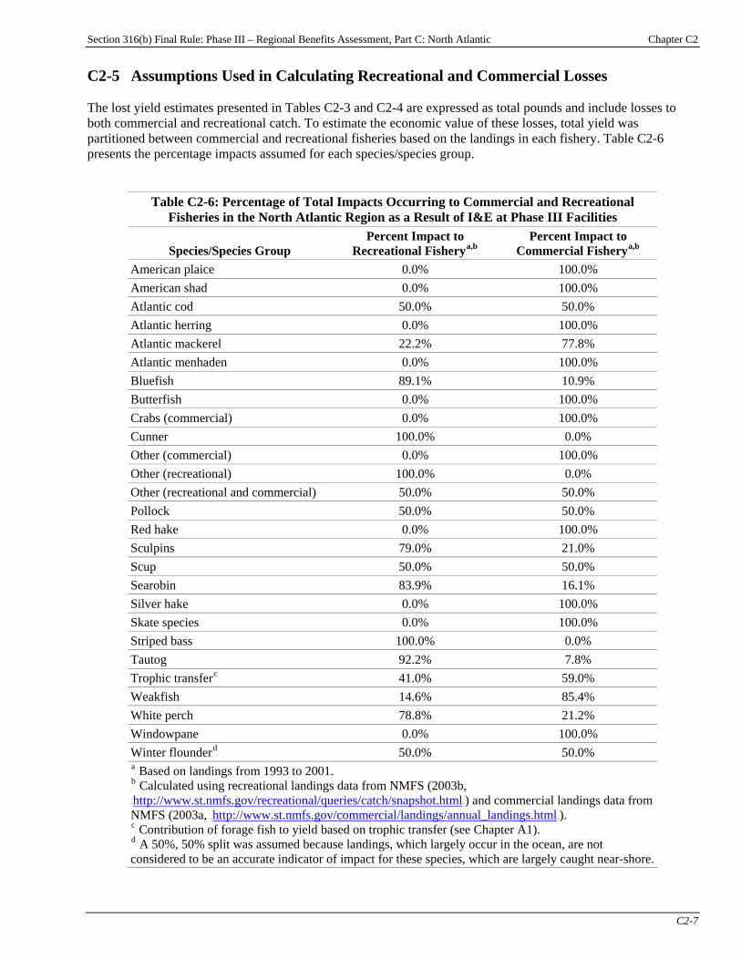
Section 316(b) Final Rule: Phase III – Regional Benefits Assessment, Part C: North Atlantic Chapter C2
C2-7
C2-5 Assumptions Used in Calculating Recreational and Commercial Losses The lost yield estimates presented in Tables C2-3 and C2-4 are expressed as total pounds and include losses to both commercial and recreational catch. To estimate the economic value of these losses, total yield was partitioned between commercial and recreational fisheries based on the landings in each fishery. Table C2-6 presents the percentage impacts assumed for each species/species group.
Table C2-6: Percentage of Total Impacts Occurring to Commercial and Recreational Fisheries in the North Atlantic Region as a Result of I&E at Phase III Facilities
Species/Species Group Percent Impact to
Recreational FisheryP
a,bP
Percent Impact to Commercial FisheryP
a,bP
American plaice 0.0% 100.0% American shad 0.0% 100.0% Atlantic cod 50.0% 50.0% Atlantic herring 0.0% 100.0% Atlantic mackerel 22.2% 77.8% Atlantic menhaden 0.0% 100.0% Bluefish 89.1% 10.9% Butterfish 0.0% 100.0% Crabs (commercial) 0.0% 100.0% Cunner 100.0% 0.0% Other (commercial) 0.0% 100.0% Other (recreational) 100.0% 0.0% Other (recreational and commercial) 50.0% 50.0% Pollock 50.0% 50.0% Red hake 0.0% 100.0% Sculpins 79.0% 21.0% Scup 50.0% 50.0% Searobin 83.9% 16.1% Silver hake 0.0% 100.0% Skate species 0.0% 100.0% Striped bass 100.0% 0.0% Tautog 92.2% 7.8% Trophic transferP
cP 41.0% 59.0%
Weakfish 14.6% 85.4% White perch 78.8% 21.2% Windowpane 0.0% 100.0% Winter flounderP
dP 50.0% 50.0%
P
aP Based on landings from 1993 to 2001.
P
bP Calculated using recreational landings data from NMFS (2003b,
HTUhttp://www.st.nmfs.gov/recreational/queries/catch/snapshot.htmlUTH) and commercial landings data from NMFS (2003a, HTUhttp://www.st.nmfs.gov/commercial/landings/annual_landings.htmlUTH). P
cP Contribution of forage fish to yield based on trophic transfer (see Chapter A1).
P
dP A 50%, 50% split was assumed because landings, which largely occur in the ocean, are not
considered to be an accurate indicator of impact for these species, which are largely caught near-shore.

Section 316(b) Final Rule: Phase III – Regional Benefits Assessment, Part C: North Atlantic Chapter C2
C2-8
See Chapter C3 for results of the commercial fishing benefits analysis and Chapter C4 for recreational fishing results. As discussed in Chapter A8, benefits were discounted to account for (1) the time to achieve compliance once a Phase III final regulation for existing facilities would have become effective, and (2) the time it takes for fish spared from I&E to reach a harvestable age. For the North Atlantic region, EPA assumes the average compliance year will be 2010 for all options.
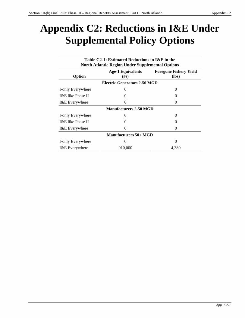
Section 316(b) Final Rule: Phase III – Regional Benefits Assessment, Part C: North Atlantic Appendix C2
App. C2-1
Appendix C2: Reductions in I&E Under Supplemental Policy Options
Table C2-1: Estimated Reductions in I&E in the North Atlantic Region Under Supplemental Options
Option Age-1 Equivalents
(#s) Foregone Fishery Yield
(lbs) Electric Generators 2-50 MGD
I-only Everywhere 0 0 I&E like Phase II 0 0 I&E Everywhere 0 0
Manufacturers 2-50 MGD I-only Everywhere 0 0 I&E like Phase II 0 0 I&E Everywhere 0 0
Manufacturers 50+ MGD I-only Everywhere 0 0 I&E Everywhere 910,000 4,380
Section 316(b) Final Rule: Phase III – Regional Benefits Assessment, Part C: North Atlantic Chapter C3
C3-1
Chapter C3: Commercial Fishing Benefits Introduction
Chapter Contents C3-1 Baseline Commercial Losses........................ C3-1 C3-2 Expected Benefits Under Regulatory Analysis Options .......................................... C3-3
C3-2.1 Commercial Fishing Benefits of the “50 MGD for All Waterbodies” Option ............................................. C3-3 C3-2.2 Commercial Fishing Benefits of the “200 MGD for All Waterbodies” Option ............................................. C3-4
C3-2.3 Commercial Fishing Benefits of the “100 MGD for Certain Waterbodies” Option ...................... C3-4
This chapter presents the results of the commercial fishing benefits analysis for the North Atlantic region. The chapter presents EPA’s estimates of baseline (i.e., current) annual commercial fishery losses from impingement and entrainment (I&E) at potentially regulated facilities in the North Atlantic region and annual reductions in these losses under the regulatory options for Phase III existing facilitiesPF
1FP:
< the “50 MGD for All Waterbodies” option, < the “200 MGD for All Waterbodies”
option, and < the “100 MGD for Certain Waterbodies”
option. The chapter then presents the estimated benefits to commercial fisheries from eliminating baseline losses from I&E, and the expected benefits under the regulatory options. Chapter A4, “Methods for Estimating Commercial Fishing Benefits,” details the methods used by EPA to estimate the commercial fishing benefits of reducing and eliminating I&E losses. EPA considered a wide range of policy options in developing this regulation. In addition to the regulatory options, EPA evaluated several supplemental options. Appendix C3 presents results of the commercial fishing benefits analysis for the supplemental options. For additional information on the options, please see the TDD. C3-1 Baseline Commercial Losses Table C3-1 provides EPA’s estimate of the value of gross revenues lost in commercial fisheries resulting from the impingement of aquatic species at facilities in the North Atlantic region. Table C3-2 displays this information for entrainment. Total annualized revenue losses are approximately $1,536 (undiscounted)
P
1P See the Introduction to this report for a description of the regulatory options.
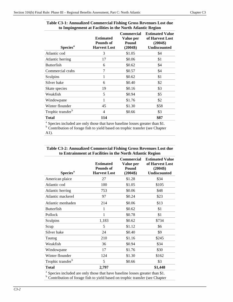
Section 316(b) Final Rule: Phase III – Regional Benefits Assessment, Part C: North Atlantic Chapter C3
C3-2
Table C3-1: Annualized Commercial Fishing Gross Revenues Lost due to Impingement at Facilities in the North Atlantic Region
SpeciesP
aP
Estimated Pounds of
Harvest Lost
Commercial Value per
Pound (2004$)
Estimated Value of Harvest Lost
(2004$) Undiscounted
Atlantic cod 3 $1.05 $4 Atlantic herring 17 $0.06 $1 Butterfish 6 $0.62 $4 Commercial crabs 7 $0.57 $4 Sculpins 1 $0.62 $1 Silver hake 6 $0.40 $2 Skate species 19 $0.16 $3 Weakfish 5 $0.94 $5 Windowpane 1 $1.76 $2 Winter flounder 45 $1.30 $58 Trophic transferP
bP 4 $0.66 $3
Total 114 $87 P
aP Species included are only those that have baseline losses greater than $1.
P
bP Contribution of forage fish to yield based on trophic transfer (see Chapter
A1).
Table C3-2: Annualized Commercial Fishing Gross Revenues Lost due to Entrainment at Facilities in the North Atlantic Region
SpeciesP
aP
Estimated Pounds of
Harvest Lost
Commercial Value per
Pound (2004$)
Estimated Value of Harvest Lost
(2004$) Undiscounted
American plaice 27 $1.28 $34 Atlantic cod 100 $1.05 $105 Atlantic herring 753 $0.06 $48 Atlantic mackerel 97 $0.24 $23
Atlantic menhaden 214 $0.06 $13 Butterfish 1 $0.62 $1 Pollock 1 $0.78 $1 Sculpins 1,183 $0.62 $734 Scup 5 $1.12 $6 Silver hake 24 $0.40 $9 Tautog 210 $1.16 $245 Weakfish 36 $0.94 $34 Windowpane 17 $1.76 $30 Winter flounder 124 $1.30 $162 Trophic transferP
bP 5 $0.66 $3
Total 2,797 $1,448 P
aP Species included are only those that have baseline losses greater than $1.
P
bP Contribution of forage fish to yield based on trophic transfer (see Chapter

Section 316(b) Final Rule: Phase III – Regional Benefits Assessment, Part C: North Atlantic Chapter C3
C3-3
Table C3-2: Annualized Commercial Fishing Gross Revenues Lost due to Entrainment at Facilities in the North Atlantic Region
SpeciesP
aP
Estimated Pounds of
Harvest Lost
Commercial Value per
Pound (2004$)
Estimated Value of Harvest Lost
(2004$) Undiscounted
A1). C3-2 Expected Benefits Under Regulatory Analysis Options As described in Chapter A4, EPA estimates for North Atlantic that, depending on species, 0 to 82% of the gross revenue losses represent surplus losses to producers, assuming no change in prices or fishing costs. Earlier EPA analysis assumed a rate of 40%. The 0% estimate, of course, results in loss estimates of $0. The expected reductions in I&E attributable to changes at facilities required by the “50 MGD for All Waterbodies” option (50 MGD All option) are 0% for impingement and 39.7% for entrainment; the expected reductions for the “200 MGD for All Waterbodies” option (200 MGD All option) are 0% for impingement and 8.4% for entrainment; and the expected reductions for the “100 MGD for Certain Waterbodies” option (100 MGD CWB option) are 0% for impingement and 32.1% for entrainment. Total annualized benefits are estimated by applying these estimated reductions to the annual baseline producer surplus loss. As presented in Tables C3-3, C3-4, and C3-5, this results in total annualized benefits of up to approximately $138 for the 50 MGD All option, $28 for the 200 MGD All option, and $113 for the 100 MGD CWB option, assuming a 3% discount rate and a species specific net benefits ratio.TPF
2FPT
C3-2.1 Commercial Fishing Benefits of the “50 MGD for All Waterbodies” Option Table C3-3 shows EPA’s analysis of the commercial benefits of the “50 MGD for All Waterbodies” option for the North Atlantic region. The table shows that this option, assuming a species-specific net benefits ratio, will result in undiscounted total annualized commercial benefits of approximately $169. When evaluated at 3% and 7% discount rates, the annualized commercial benefits are $138 and $107, respectively.
Table C3-3: Annualized Commercial Fishing Benefits Attributable to the 50 MGD All Option at Facilities in the North Atlantic Region (2004$)P
aP
Impingement Entrainment Total Baseline loss — gross revenue
Undiscounted $89 $1,447 $1,536 Producer surplus lost — 0% $0 $0 $0 Producer surplus lost — (gross revenue * species-specific net benefits ratio)
Undiscounted $57 $425 $482 Expected reduction due to rule 0% 39.7% Benefits attributable to rule — 0% $0 $0 $0 Benefits attributable to rule — species-specific net benefits ratio
Undiscounted $169 3% discount rate $138
TP
2PT The net benefits ratio is the fractional share of gross revenue associated with net benefits, by gear and vessel
type. See Chapter A4, section A4-10, for a description of the species-specific net benefits ratios and how they are calculated.

Section 316(b) Final Rule: Phase III – Regional Benefits Assessment, Part C: North Atlantic Chapter C3
C3-4
7% discount rate $107 P
aP Annualized benefits represent the value of all commercial benefits generated over the time
frame of the analysis, discounted to 2007, and then annualized over a 30 year period. For a more detailed discussion of the discounting methodology, refer to Chapter A8, and see Chapter I1 for a timeline of benefits.
C3-2.2 Commercial Fishing Benefits of the “200 MGD for All Waterbodies” Option Table C3-4 shows EPA’s analysis of the commercial benefits of the “200 MGD for All Waterbodies” option for the North Atlantic region. The table shows that this option, assuming a species-specific net benefits ratio, will result in undiscounted total annualized commercial benefits of approximately $36. When evaluated at 3% and 7% discount rates, the annualized commercial benefits are $28 and $21, respectively.
Table C3-4: Annualized Commercial Fishing Benefits Attributable to the 200 MGD All Option at Facilities in the North Atlantic Region (2004$)P
aP
Impingement Entrainment Total Baseline loss — gross revenue
Undiscounted $89 $1,447 $1,536 Producer surplus lost — 0% $0 $0 $0 Producer surplus lost — (gross revenue * species-specific net benefits ratio)
Undiscounted $57 $425 $482 Expected reduction due to rule 0 8.4% Benefits attributable to rule — 0% $0 $0 $0 Benefits attributable to rule — species-specific net benefits ratio
Undiscounted $36 3% discount rate $28 7% discount rate $21
P
aP Annualized benefits represent the value of all commercial benefits generated over the time
frame of the analysis, discounted to 2007, and then annualized over a 30 year period. For a more detailed discussion of the discounting methodology, refer to Chapter A8, and see Chapter I1 for a timeline of benefits.
C3-2.3 Commercial Fishing Benefits of the “100 MGD for Certain Waterbodies” Option Table C3-5 shows EPA’s analysis of the commercial benefits of the “100 MGD for Certain Waterbodies” option for the North Atlantic region. The table shows that this option, assuming a species-specific net benefits ratio, will result in undiscounted total annualized commercial benefits of approximately $137. When evaluated at 3% and 7% discount rates, the annualized commercial benefits are $113 and $88, respectively.

Section 316(b) Final Rule: Phase III – Regional Benefits Assessment, Part C: North Atlantic Chapter C3
C3-5
Table C3-5: Annualized Commercial Fishing Benefits Attributable to the 100 MGD CWB Option at Facilities in the North Atlantic Region (2004$)P
aP
Impingement Entrainment Total Baseline loss — gross revenue
Undiscounted $89 $1,447 $1,536 Producer surplus lost — 0% $0 $0 $0 Producer surplus lost — (gross revenue * species-specific net benefits ratio)
Undiscounted $57 $425 $482 Expected reduction due to rule 0% 32.1% Benefits attributable to rule — 0% $0 $0 $0 Benefits attributable to rule — species-specific net benefits ratio
Undiscounted $137 3% discount rate $113 7% discount rate $88
P
aP Annualized benefits represent the value of all commercial benefits generated over the time
frame of the analysis, discounted to 2007, and then annualized over a 30 year period. For a more detailed discussion of the discounting methodology, refer to Chapter A8, and see Chapter I1 for a timeline of benefits.

Section 316(b) Final Rule: Phase III – Regional Benefits Assessment, Part C: North Atlantic Appendix C3
App. C3-1
Appendix C3: Commercial Fishing Benefits Under Supplemental Policy Options
Introduction Chapter C3 presents EPA’s estimates of the commercial benefits of the regulatory options for the section 316(b) rule for Phase III facilities in the North Atlantic region. To facilitate comparisons among the options, this appendix presents estimates of the commercial fishing benefits of several supplemental options that EPA evaluated in preparation for this rule:
Appendix Contents C3-1 Commercial Fishing Benefits of the Supplemental Options ................................ C3-2
< “Electric Generators 2-50 MGD I-only Everywhere” option; < “Electric Generators 2-50 MGD I&E like Phase II” option; < “Electric Generators 2-50 MGD I&E Everywhere” option; < “Manufacturers 2-50 MGD I-only Everywhere” option; < “Manufacturers 2-50 MGD I&E like Phase II” option; < “Manufacturers 2-50 MGD I&E Everywhere” option; < “Manufacturers 50+ MGD I-only Everywhere” option; and < “Manufacturers 50+ MGD I&E Everywhere” option.
Commercial fishing benefits presented in this chapter were estimated using the benefit transfer approach discussed in Chapter C3 and in Chapter A4, “Methods for Estimating Commercial Fishing Benefits.”
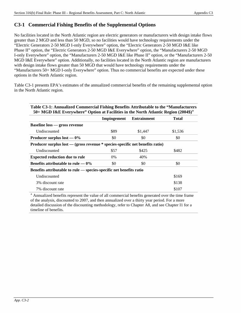
Section 316(b) Final Rule: Phase III – Regional Benefits Assessment, Part C: North Atlantic Appendix C3
App. C3-2
C3-1 Commercial Fishing Benefits of the Supplemental Options No facilities located in the North Atlantic region are electric generators or manufacturers with design intake flows greater than 2 MGD and less than 50 MGD, so no facilities would have technology requirements under the “Electric Generators 2-50 MGD I-only Everywhere” option, the “Electric Generators 2-50 MGD I&E like Phase II” option, the “Electric Generators 2-50 MGD I&E Everywhere” option, the “Manufacturers 2-50 MGD I-only Everywhere” option, the “Manufacturers 2-50 MGD I&E like Phase II” option, or the “Manufacturers 2-50 MGD I&E Everywhere” option. Additionally, no facilities located in the North Atlantic region are manufacturers with design intake flows greater than 50 MGD that would have technology requirements under the “Manufacturers 50+ MGD I-only Everywhere” option. Thus no commercial benefits are expected under these options in the North Atlantic region. Table C3-1 presents EPA’s estimates of the annualized commercial benefits of the remaining supplemental option in the North Atlantic region.
Table C3-1: Annualized Commercial Fishing Benefits Attributable to the “Manufacturers 50+ MGD I&E Everywhere” Option at Facilities in the North Atlantic Region (2004$)P
aP
Impingement Entrainment Total Baseline loss — gross revenue
Undiscounted $89 $1,447 $1,536 Producer surplus lost — 0% $0 $0 $0 Producer surplus lost — (gross revenue * species-specific net benefits ratio)
Undiscounted $57 $425 $482 Expected reduction due to rule 0% 40% Benefits attributable to rule — 0% $0 $0 $0 Benefits attributable to rule — species-specific net benefits ratio
Undiscounted $169 3% discount rate $138 7% discount rate $107
P
aP Annualized benefits represent the value of all commercial benefits generated over the time frame
of the analysis, discounted to 2007, and then annualized over a thirty year period. For a more detailed discussion of the discounting methodology, refer to Chapter A8, and see Chapter I1 for a timeline of benefits.

Section 316(b) Final Rule: Phase III – Regional Benefits Assessment, Part C: North Atlantic Chapter C4
C4-1
Chapter C4: Recreational Use Benefits
Chapter Contents C4-1 Benefit Transfer Approach Based on Meta-Analysis............................................... C4-1 C4-1.1 Baseline Losses and Reductions in Recreational Fishery Losses Under the Regulatory Options .................. C4-2 C4-1.2 Recreational Fishing Benefits from Eliminating Baseline I&E Losses.............................................. C4-3 C4-1.3 Recreational Fishing Benefits of the “50 MGD for All Waterbodies” Option.............................................. C4-4 C4-1.4 Recreational Fishing Benefits of the “200 MGD for All Waterbodies” Option.............................................. C4-5 C4-1.5 Recreational Fishing Benefits of the “100 MGD for Certain Waterbodies” Option.............................................. C4-6 C4-2 Limitations and Uncertainty ......................... C4-7
Introduction This chapter presents the results of the recreational fishing benefits analysis for the North Atlantic region. The chapter presents EPA’s estimates of baseline (i.e., current) annual recreational fishery losses from impingement and entrainment (I&E) at potentially regulated facilities in the North Atlantic region and annual reductions in these losses under the regulatory options for Phase III existing facilitiesPF
1FP:
< the “50 MGD for All Waterbodies” option, < the “200 MGD for All Waterbodies”
option, and < the “100 MGD for Certain Waterbodies”
option. The chapter then presents the estimated welfare gain to North Atlantic anglers from eliminating baseline recreational fishing losses from I&E and the expected benefits under the regulatory options. EPA estimated the recreational benefits of reducing and eliminating I&E losses using a benefit transfer methodology based on a meta-analysis of the marginal value of catching different species of fish. This meta-analysis is discussed in detail in Chapter A5, “Recreational Fishing Benefits Methodology.” EPA considered a wide range of policy options in developing this regulation. In addition to the regulatory options, EPA evaluated several supplemental options. Appendix C4 presents results of the recreational fishing benefits analysis for the supplemental options. For more information on the options, please see the TDD. C4-1 Benefit Transfer Approach Based on Meta-Analysis EPA estimated the recreational welfare gain from the reduction in annual I&E losses expected under the policy options, and the welfare gain from eliminating I&E at potentially regulated facilities, using a benefit transfer approach. As discussed in Chapter A5, the Agency used a meta-analysis regression equation to estimate the marginal recreational value per additional fish caught by anglers, for different species in different regions. Since I&E at potentially regulated facilities affects a variety of species, EPA assigned each species with I&E losses to one of the general species groups used in the meta-analysis. The Agency then calculated the economic value of reducing or eliminating baseline I&E losses, for each species group, by multiplying the value per fish for that species group by the number of fish in the group that are lost in the baseline or saved under the policy options.PF
2FP
P
1P See the Introduction to this report for a description of the primary analysis options.
P
2P The estimates of I&E presented in this chapter include only the fraction of impinged and entrained recreational
fish that would be caught by anglers. The total amount of I&E of recreational species is actually much higher.

Section 316(b) Final Rule: Phase III – Regional Benefits Assessment, Part C: North Atlantic Chapter C4
C4-2
In general, the fit between the species with I&E losses and the species groups in the meta-analysis was good. However, EPA’s estimates of baseline I&E losses and reductions in I&E under the policy options included losses of “unidentified” species. The “unidentified” group includes fish lost indirectly through trophic transfer, as well as species for which no species information was available.PF
3FP Rather than using the meta-analysis regression to try to
predict the value per fish for an “unidentified” species, EPA assumed that per-fish values for these species can be approximated by the weighted average value per fish for all species affected by I&E in the North Atlantic region.PF
4FP
C4-1.1 Baseline Losses and Reductions in Recreational Fishery Losses Under the Regulatory Options Table C4-1 presents EPA’s estimates of baseline (i.e., current) annual recreational I&E losses at potentially regulated facilities, and annual reductions in these losses under each of the regulatory options, in the North Atlantic region. The table shows that total baseline losses to recreational fisheries are 20.8 thousand fish per year. In comparison, the “50 MGD for All Waterbodies” option prevents losses of 8.2 thousand fish per year, the “200 MGD for All Waterbodies” option prevents losses of 1.7 thousand fish per year, and the “100 MGD for Certain Waterbodies” option prevents losses of 6.7 thousand fish per year. Of all the affected species, sculpin and cunner have the highest losses in the baseline and the highest prevented losses under the regulatory options.
P
3P In addition to recreational fish that are lost because they are impinged or entrained, some recreational fish are lost
because the forage fish that they feed on are impinged or entrained, and thus removed from the food chain. These trophic transfer losses of recreational species are included in EPA’s estimates of total I&E losses. Since it is difficult to predict which recreational species would be affected by losses of forage fish, these losses are classified as “unidentified” recreational species. Also included in the “unidentified” group are losses of fish that were reported by facilities without information about their exact species.
P
4P EPA used the estimated level of baseline recreational losses for each species group as a weighting factor.
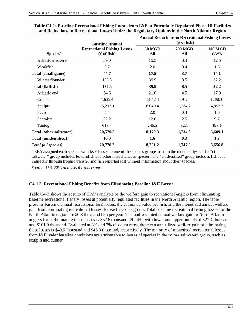
Section 316(b) Final Rule: Phase III – Regional Benefits Assessment, Part C: North Atlantic Chapter C4
C4-3
Table C4-1: Baseline Recreational Fishing Losses from I&E at Potentially Regulated Phase III Facilities and Reductions in Recreational Losses Under the Regulatory Options in the North Atlantic Region
Annual Reductions in Recreational Fishing Losses (# of fish)
SpeciesP
aP
Baseline Annual Recreational Fishing Losses
(# of fish) 50 MGD
All 200 MGD
All 100 MGD
CWB Atlantic mackerel 39.0 15.5 3.3 12.5 Weakfish 5.7 2.0 0.4 1.6
Total (small game) 44.7 17.5 3.7 14.1 Winter flounder 136.5 39.9 8.5 32.2
Total (flatfish) 136.5 39.9 8.5 32.2 Atlantic cod 54.6 21.0 4.5 17.0 Cunner 4,635.4 1,842.4 391.1 1,490.0 Sculpin 15,233.1 6,049.4 1,284.2 4,892.3 Scup 5.4 2.0 0.4 1.6 Searobin 32.2 12.0 2.5 9.7 Tautog 618.4 245.5 52.1 198.6
Total (other saltwater) 20,579.2 8,172.3 1,734.8 6,609.1 Total (unidentified) 10.0 1.6 0.3 1.3 Total (all species) 20,770.3 8,231.2 1,747.3 6,656.8 P
aP EPA assigned each species with I&E losses to one of the species groups used in the meta-analysis. The “other
saltwater” group includes bottomfish and other miscellaneous species. The “unidentified” group includes fish lost indirectly through trophic transfer and fish reported lost without information about their species. Source: U.S. EPA analysis for this report.
C4-1.2 Recreational Fishing Benefits from Eliminating Baseline I&E Losses Table C4-2 shows the results of EPA’s analysis of the welfare gain to recreational anglers from eliminating baseline recreational fishery losses at potentially regulated facilities in the North Atlantic region. The table presents baseline annual recreational I&E losses, the estimated value per fish, and the monetized annual welfare gain from eliminating recreational losses, for each species group. Total baseline recreational fishing losses for the North Atlantic region are 20.8 thousand fish per year. The undiscounted annual welfare gain to North Atlantic anglers from eliminating these losses is $52.6 thousand (2004$), with lower and upper bounds of $27.4 thousand and $101.0 thousand. Evaluated at 3% and 7% discount rates, the mean annualized welfare gain of eliminating these losses is $49.5 thousand and $45.9 thousand, respectively. The majority of monetized recreational losses from I&E under baseline conditions are attributable to losses of species in the “other saltwater” group, such as sculpin and cunner.
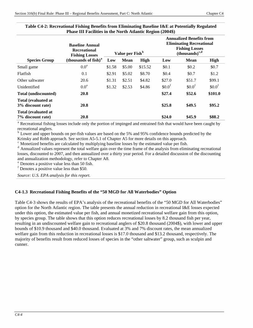
Section 316(b) Final Rule: Phase III – Regional Benefits Assessment, Part C: North Atlantic Chapter C4
C4-4
Table C4-2: Recreational Fishing Benefits from Eliminating Baseline I&E at Potentially Regulated Phase III Facilities in the North Atlantic Region (2004$)
Value per FishP
bP
Annualized Benefits from Eliminating Recreational
Fishing Losses (thousands)P
c,dP
Species Group
Baseline Annual Recreational
Fishing Losses (thousands of fish)P
aP Low Mean High Low Mean High
Small game 0.0P
eP $1.58 $5.00 $15.52 $0.1 $0.2 $0.7
Flatfish 0.1 $2.91 $5.02 $8.70 $0.4 $0.7 $1.2 Other saltwater 20.6 $1.31 $2.51 $4.82 $27.0 $51.7 $99.1 Unidentified 0.0P
eP $1.32 $2.53 $4.86 $0.0P
fP $0.0P
fP $0.0P
fP
Total (undiscounted) 20.8 $27.4 $52.6 $101.0 Total (evaluated at 3% discount rate) 20.8 $25.8 $49.5 $95.2 Total (evaluated at 7% discount rate) 20.8 $24.0 $45.9 $88.2 P
aP Recreational fishing losses include only the portion of impinged and entrained fish that would have been caught by
recreational anglers. P
bP Lower and upper bounds on per-fish values are based on the 5% and 95% confidence bounds predicted by the
Krinsky and Robb approach. See section A5-5.1 of Chapter A5 for more details on this approach. P
cP Monetized benefits are calculated by multiplying baseline losses by the estimated value per fish.
P
dP Annualized values represent the total welfare gain over the time frame of the analysis from eliminating recreational
losses, discounted to 2007, and then annualized over a thirty year period. For a detailed discussion of the discounting and annualization methodology, refer to Chapter A8. P
eP Denotes a positive value less than 50 fish.
P
fP Denotes a positive value less than $50.
Source: U.S. EPA analysis for this report. C4-1.3 Recreational Fishing Benefits of the “50 MGD for All Waterbodies” Option Table C4-3 shows the results of EPA’s analysis of the recreational benefits of the “50 MGD for All Waterbodies” option for the North Atlantic region. The table presents the annual reduction in recreational I&E losses expected under this option, the estimated value per fish, and annual monetized recreational welfare gain from this option, by species group. The table shows that this option reduces recreational losses by 8.2 thousand fish per year, resulting in an undiscounted welfare gain to recreational anglers of $20.8 thousand (2004$), with lower and upper bounds of $10.9 thousand and $40.0 thousand. Evaluated at 3% and 7% discount rates, the mean annualized welfare gain from this reduction in recreational losses is $17.0 thousand and $13.2 thousand, respectively. The majority of benefits result from reduced losses of species in the “other saltwater” group, such as sculpin and cunner.

Section 316(b) Final Rule: Phase III – Regional Benefits Assessment, Part C: North Atlantic Chapter C4
C4-5
Table C4-3: Recreational Fishing Benefits of the “50 MGD for All Waterbodies” Option in the North Atlantic Region (2004$)
Value per FishP
bP
Annualized Recreational Fishing Benefits (thousands)P
c,dP
Species Group
Annual Reduction in Recreational Fishing Losses
(thousands of fish)P
aP Low Mean High Low Mean High
Small game 0.0P
eP $1.58 $5.00 $15.52 $0.0P
fP $0.1 $0.3
Flatfish 0.0P
eP $2.91 $5.02 $8.70 $0.1 $0.2 $0.3
Other saltwater 8.2 $1.31 $2.51 $4.82 $10.7 $20.5 $39.4 Unidentified 0.0P
eP $1.32 $2.53 $4.86 $0.0P
fP $0.0P
fP $0.0P
fP
Total (undiscounted) 8.2 $10.9 $20.8 $40.0 Total (evaluated at 3% discount rate) 8.2 $8.9 $17.0 $32.7 Total (evaluated at 7% discount rate) 8.2 $6.9 $13.2 $25.3 P
aP Recreational fishing losses include only the portion of impinged and entrained fish that would have been caught by
recreational anglers. P
bP Lower and upper bounds on per-fish values are based on the 5% and 95% confidence bounds predicted by the
Krinsky and Robb approach. See section A5-5.1 of Chapter A5 for more details on this approach. P
cP Monetized benefits are calculated by multiplying the annual reduction in recreational losses by the estimated value
per fish. P
dP Annualized benefits represent the value of all recreational benefits generated over the time frame of the analysis,
discounted to 2007, and then annualized over a thirty year period. For a detailed discussion of the discounting and annualization methodology, refer to Chapter A8. P
eP Denotes a positive value less than 50 fish.
P
fP Denotes a positive value less than $50.
Source: U.S. EPA analysis for this report. C4-1.4 Recreational Fishing Benefits of the “200 MGD for All Waterbodies” Option Table C4-4 shows the results of EPA’s analysis of the recreational benefits of the “200 MGD for All Waterbodies” option for the North Atlantic region. The table presents the annual reduction in recreational I&E losses expected under this option, the estimated value per fish, and annual monetized recreational welfare gain from this option, by species group. The table shows that this option reduces recreational losses by 1.7 thousand fish per year, resulting in an undiscounted welfare gain to recreational anglers of $4.4 thousand (2004$), with lower and upper bounds of $2.3 thousand and $8.5 thousand. Evaluated at 3% and 7% discount rates, the mean annualized welfare gain from this reduction in recreational losses is $3.5 thousand and $2.6 thousand, respectively. The majority of benefits result from reduced losses of species in the “other saltwater” group, such as sculpin and cunner.

Section 316(b) Final Rule: Phase III – Regional Benefits Assessment, Part C: North Atlantic Chapter C4
C4-6
Table C4-4: Recreational Fishing Benefits of the “200 MGD for All Waterbodies” Option in the North Atlantic Region (2004$)
Value per FishP
bP
Annualized Recreational Fishing Benefits (thousands)P
c,dP
Species Group
Annual Reduction in Recreational Fishing Losses
(thousands of fish)P
aP Low Mean High Low Mean High
Small game 0.0P
eP $1.58 $5.00 $15.52 $0.0P
fP $0.0P
fP $0.1
Flatfish 0.0P
eP $2.91 $5.02 $8.70 $0.0P
fP $0.0P
fP $0.1
Other saltwater 1.7 $1.31 $2.51 $4.82 $2.3 $4.4 $8.4 Unidentified 0.0P
eP $1.32 $2.53 $4.86 $0.0P
fP $0.0P
fP $0.0P
fP
Total (undiscounted) 1.7 $2.3 $4.4 $8.5 Total (evaluated at 3% discount rate) 1.7 $1.8 $3.5 $6.7 Total (evaluated at 7% discount rate) 1.7 $1.3 $2.6 $4.9 P
aP Recreational fishing losses include only the portion of impinged and entrained fish that would have been caught by
recreational anglers. P
bP Lower and upper bounds on per-fish values are based on the 5% and 95% confidence bounds predicted by the
Krinsky and Robb approach. See section A5-5.1 of Chapter A5 for more details on this approach. P
cP Monetized benefits are calculated by multiplying the annual reduction in recreational losses by the estimated value
per fish. P
dP Annualized benefits represent the value of all recreational benefits generated over the time frame of the analysis,
discounted to 2007, and then annualized over a thirty year period. For a detailed discussion of the discounting and annualization methodology, refer to Chapter A8. P
eP Denotes a positive value less than 50 fish.
P
fP Denotes a positive value less than $50.
Source: U.S. EPA analysis for this report. C4-1.5 Recreational Fishing Benefits of the “100 MGD for Certain Waterbodies” Option Table C4-5 shows the results of EPA’s analysis of the recreational benefits of the “100 MGD for Certain Waterbodies” option for the North Atlantic region. The table presents the annual reduction in recreational I&E losses expected under this option, the estimated value per fish, and annual monetized recreational welfare gain from this option, by species group. The table shows that this option reduces recreational losses by 6.7 thousand fish per year, resulting in an undiscounted welfare gain to recreational anglers of $16.8 thousand (2004$), with lower and upper bounds of $8.8 thousand and $32.3 thousand. Evaluated at 3% and 7% discount rates, the mean annualized welfare gain from this reduction in recreational losses is $13.9 thousand and $10.8 thousand, respectively. The majority of benefits result from reduced losses of species in the “other saltwater” group, such as sculpin and cunner.

Section 316(b) Final Rule: Phase III – Regional Benefits Assessment, Part C: North Atlantic Chapter C4
C4-7
Table C4-5: Recreational Fishing Benefits of the “100 MGD for Certain Waterbodies” Option in the North Atlantic Region (2004$)
Value per FishP
bP
Annualized Recreational Fishing Benefits (thousands)P
c,dP
Species Group
Annual Reduction in Recreational Fishing Losses
(thousands of fish)P
aP Low Mean High Low Mean High
Small game 0.0P
eP $1.58 $5.00 $15.52 $0.0P
fP $0.1 $0.2
Flatfish 0.0P
eP $2.91 $5.02 $8.70 $0.1 $0.2 $0.3
Other saltwater 6.6 $1.31 $2.51 $4.82 $8.7 $16.6 $31.8 Unidentified 0.0P
eP $1.32 $2.53 $4.86 $0.0P
fP $0.0P
fP $0.0P
fP
Total (undiscounted) 6.7 $8.8 $16.8 $32.3 Total (evaluated at 3% discount rate) 6.7 $7.2 $13.9 $26.6 Total (evaluated at 7% discount rate) 6.7 $5.7 $10.8 $20.8 P
aP Recreational fishing losses include only the portion of impinged and entrained fish that would have been caught by
recreational anglers. P
bP Lower and upper bounds on per-fish values are based on the 5% and 95% confidence bounds predicted by the
Krinsky and Robb approach. See section A5-5.1 of Chapter A5 for more details on this approach. P
cP Monetized benefits are calculated by multiplying the annual reduction in recreational losses by the estimated value
per fish. P
dP Annualized benefits represent the value of all recreational benefits generated over the time frame of the analysis,
discounted to 2007, and then annualized over a thirty year period. For a detailed discussion of the discounting and annualization methodology, refer to Chapter A8. P
eP Denotes a positive value less than 50 fish.
P
fP Denotes a positive value less than $50.
Source: U.S. EPA analysis for this report. C4-2 Limitations and Uncertainty The results of the benefit transfer based on a meta-analysis represent EPA’s best estimate of the recreational benefits of the regulatory options. Nonetheless, there are a number of limitations and uncertainties inherent in these estimates. General limitations pertaining to the development of the meta-analysis model, the use of the model to estimate per-fish values, and the validity of the benefit transfer are discussed in section A5-3.3e and section A5-5.3 of Chapter A5.
Section 316(b) Final Rule: Phase III – Regional Benefits Assessment, Part C: North Atlantic Appendix C4
App. C4-1
Appendix C4: Recreational Use Benefits Under Supplemental Policy Options
Introduction
Appendix Contents C4-1 Recreational Fishing Benefits of the Supplemental Options .................................C4-1 C4-1.1 Estimated Reductions in Recreational Fishing Losses
Under the Supplemental Options...C4-1 C4-1.2 Recreational Fishing Benefits of the Supplemental Options .............C4-3 C4-2 Comparison of Recreational Fishing Benefits by Option ......................................C4-4
Chapter C4 presents EPA’s estimates of the recreational benefits of the regulatory options for the section 316(b) rule for Phase III facilities in the North Atlantic region. To facilitate comparisons among the options, this appendix presents estimates of the recreational fishing benefits of several supplemental options that EPA evaluated in preparation for this rule:
< “Electric Generators 2-50 MGD I-only Everywhere” option;
< “Electric Generators 2-50 MGD I&E like Phase II” option;
< “Electric Generators 2-50 MGD I&E Everywhere” option; < “Manufacturers 2-50 MGD I-only Everywhere” option; < “Manufacturers 2-50 MGD I&E like Phase II” option; < “Manufacturers 2-50 MGD I&E Everywhere” option; < “Manufacturers 50+ MGD I-only Everywhere” option; and < “Manufacturers 50+ MGD I&E Everywhere” option.
Recreational fishing benefits presented in this chapter were estimated using the benefit transfer approach discussed in Chapter C4 and in Chapter A5, “Recreational Fishing Benefits Methodology.” C4-1 Recreational Fishing Benefits of the Supplemental Options C4-1.1 Estimated Reductions in Recreational Fishing Losses Under the Supplemental Options Table C4-1 presents EPA’s estimates of the annual reduction in baseline (i.e., current) recreational fishing losses from impingement and entrainment (I&E) in the North Atlantic region under the supplemental options. For more information on the options, please see the TDD.
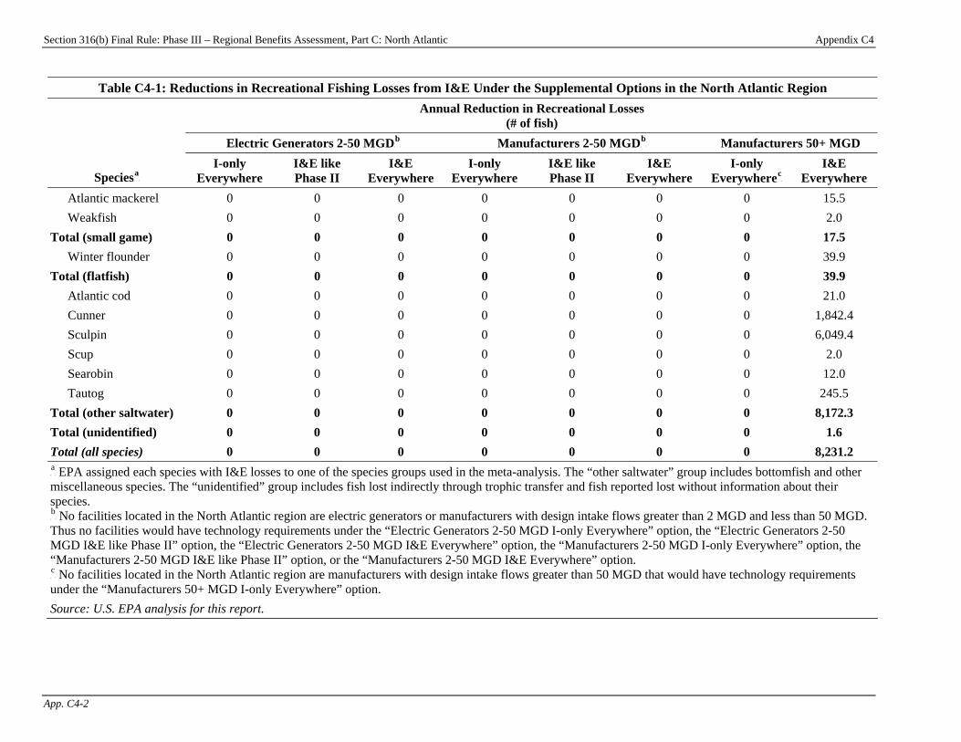
Section 316(b) Final Rule: Phase III – Regional Benefits Assessment, Part C: North Atlantic Appendix C4
App. C4-2
Table C4-1: Reductions in Recreational Fishing Losses from I&E Under the Supplemental Options in the North Atlantic Region Annual Reduction in Recreational Losses
(# of fish) Electric Generators 2-50 MGDP
bP Manufacturers 2-50 MGDP
bP Manufacturers 50+ MGD
SpeciesP
aP
I-only Everywhere
I&E like Phase II
I&E Everywhere
I-only Everywhere
I&E like Phase II
I&E Everywhere
I-only EverywhereP
cP
I&E Everywhere
Atlantic mackerel 0 0 0 0 0 0 0 15.5 Weakfish 0 0 0 0 0 0 0 2.0
Total (small game) 0 0 0 0 0 0 0 17.5 Winter flounder 0 0 0 0 0 0 0 39.9
Total (flatfish) 0 0 0 0 0 0 0 39.9 Atlantic cod 0 0 0 0 0 0 0 21.0 Cunner 0 0 0 0 0 0 0 1,842.4 Sculpin 0 0 0 0 0 0 0 6,049.4 Scup 0 0 0 0 0 0 0 2.0 Searobin 0 0 0 0 0 0 0 12.0 Tautog 0 0 0 0 0 0 0 245.5
Total (other saltwater) 0 0 0 0 0 0 0 8,172.3 Total (unidentified) 0 0 0 0 0 0 0 1.6 Total (all species) 0 0 0 0 0 0 0 8,231.2 P
aP EPA assigned each species with I&E losses to one of the species groups used in the meta-analysis. The “other saltwater” group includes bottomfish and other
miscellaneous species. The “unidentified” group includes fish lost indirectly through trophic transfer and fish reported lost without information about their species. P
bP No facilities located in the North Atlantic region are electric generators or manufacturers with design intake flows greater than 2 MGD and less than 50 MGD.
Thus no facilities would have technology requirements under the “Electric Generators 2-50 MGD I-only Everywhere” option, the “Electric Generators 2-50 MGD I&E like Phase II” option, the “Electric Generators 2-50 MGD I&E Everywhere” option, the “Manufacturers 2-50 MGD I-only Everywhere” option, the “Manufacturers 2-50 MGD I&E like Phase II” option, or the “Manufacturers 2-50 MGD I&E Everywhere” option. P
cP No facilities located in the North Atlantic region are manufacturers with design intake flows greater than 50 MGD that would have technology requirements
under the “Manufacturers 50+ MGD I-only Everywhere” option. Source: U.S. EPA analysis for this report.
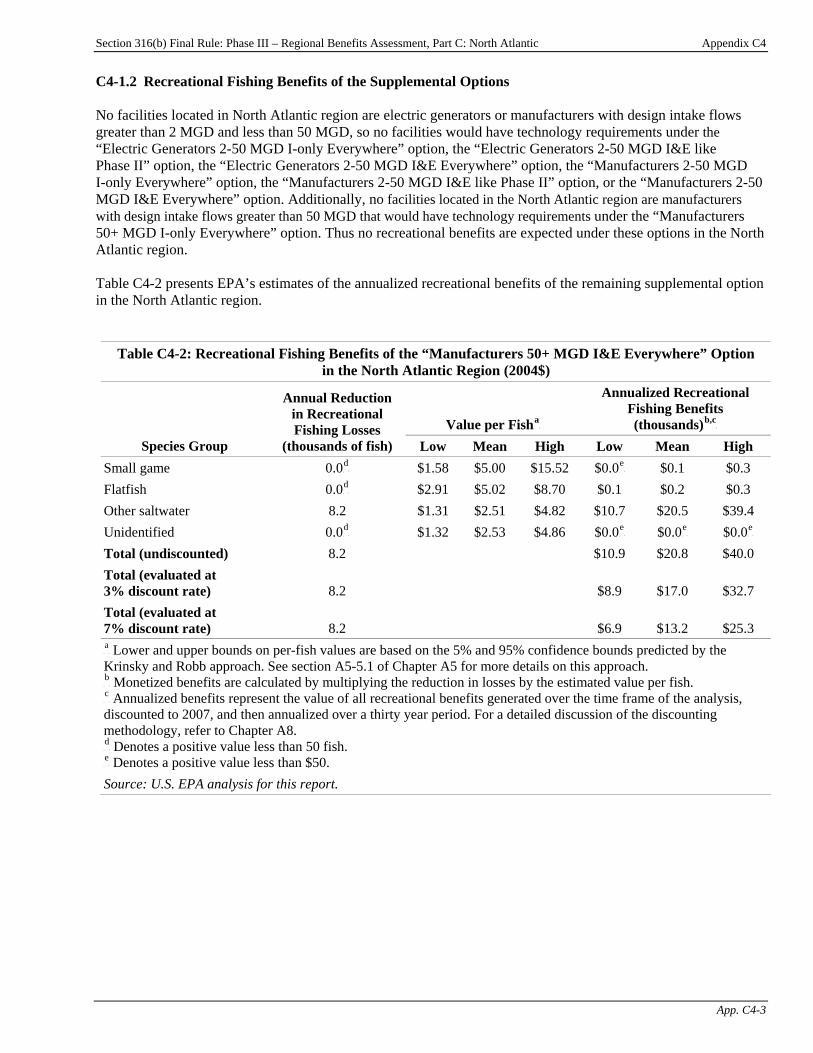
Section 316(b) Final Rule: Phase III – Regional Benefits Assessment, Part C: North Atlantic Appendix C4
App. C4-3
C4-1.2 Recreational Fishing Benefits of the Supplemental Options No facilities located in North Atlantic region are electric generators or manufacturers with design intake flows greater than 2 MGD and less than 50 MGD, so no facilities would have technology requirements under the “Electric Generators 2-50 MGD I-only Everywhere” option, the “Electric Generators 2-50 MGD I&E like Phase II” option, the “Electric Generators 2-50 MGD I&E Everywhere” option, the “Manufacturers 2-50 MGD I-only Everywhere” option, the “Manufacturers 2-50 MGD I&E like Phase II” option, or the “Manufacturers 2-50 MGD I&E Everywhere” option. Additionally, no facilities located in the North Atlantic region are manufacturers with design intake flows greater than 50 MGD that would have technology requirements under the “Manufacturers 50+ MGD I-only Everywhere” option. Thus no recreational benefits are expected under these options in the North Atlantic region. Table C4-2 presents EPA’s estimates of the annualized recreational benefits of the remaining supplemental option in the North Atlantic region.
Table C4-2: Recreational Fishing Benefits of the “Manufacturers 50+ MGD I&E Everywhere” Option in the North Atlantic Region (2004$)
Value per FishP
aP
Annualized Recreational Fishing Benefits (thousands)P
b,cP
Species Group
Annual Reduction in Recreational Fishing Losses
(thousands of fish) Low Mean High Low Mean High Small game 0.0P
dP $1.58 $5.00 $15.52 $0.0P
eP $0.1 $0.3
Flatfish 0.0P
dP $2.91 $5.02 $8.70 $0.1 $0.2 $0.3
Other saltwater 8.2 $1.31 $2.51 $4.82 $10.7 $20.5 $39.4 Unidentified 0.0P
dP $1.32 $2.53 $4.86 $0.0P
eP $0.0P
eP $0.0P
eP
Total (undiscounted) 8.2 $10.9 $20.8 $40.0 Total (evaluated at 3% discount rate) 8.2 $8.9 $17.0 $32.7 Total (evaluated at 7% discount rate) 8.2 $6.9 $13.2 $25.3 P
aP Lower and upper bounds on per-fish values are based on the 5% and 95% confidence bounds predicted by the
Krinsky and Robb approach. See section A5-5.1 of Chapter A5 for more details on this approach. P
bP Monetized benefits are calculated by multiplying the reduction in losses by the estimated value per fish.
P
cP Annualized benefits represent the value of all recreational benefits generated over the time frame of the analysis,
discounted to 2007, and then annualized over a thirty year period. For a detailed discussion of the discounting methodology, refer to Chapter A8. P
dP Denotes a positive value less than 50 fish.
P
eP Denotes a positive value less than $50.
Source: U.S. EPA analysis for this report.
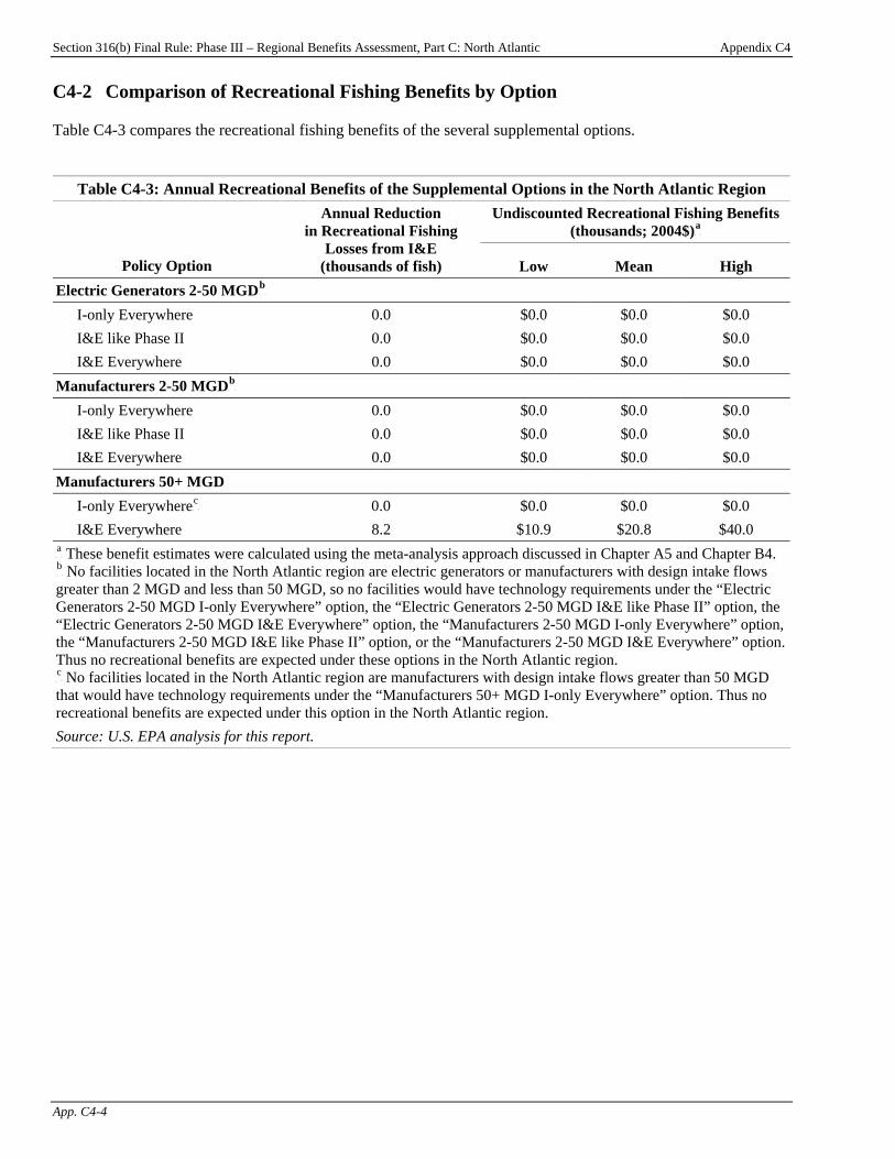
Section 316(b) Final Rule: Phase III – Regional Benefits Assessment, Part C: North Atlantic Appendix C4
App. C4-4
C4-2 Comparison of Recreational Fishing Benefits by Option Table C4-3 compares the recreational fishing benefits of the several supplemental options.
Table C4-3: Annual Recreational Benefits of the Supplemental Options in the North Atlantic Region Undiscounted Recreational Fishing Benefits
(thousands; 2004$)P
aP
Policy Option
Annual Reduction in Recreational Fishing
Losses from I&E (thousands of fish) Low Mean High
Electric Generators 2-50 MGDP
bP
I-only Everywhere 0.0 $0.0 $0.0 $0.0 I&E like Phase II 0.0 $0.0 $0.0 $0.0 I&E Everywhere 0.0 $0.0 $0.0 $0.0
Manufacturers 2-50 MGDP
bP
I-only Everywhere 0.0 $0.0 $0.0 $0.0 I&E like Phase II 0.0 $0.0 $0.0 $0.0 I&E Everywhere 0.0 $0.0 $0.0 $0.0
Manufacturers 50+ MGD I-only EverywhereP
cP 0.0 $0.0 $0.0 $0.0
I&E Everywhere 8.2 $10.9 $20.8 $40.0 P
aP These benefit estimates were calculated using the meta-analysis approach discussed in Chapter A5 and Chapter B4.
P
bP No facilities located in the North Atlantic region are electric generators or manufacturers with design intake flows
greater than 2 MGD and less than 50 MGD, so no facilities would have technology requirements under the “Electric Generators 2-50 MGD I-only Everywhere” option, the “Electric Generators 2-50 MGD I&E like Phase II” option, the “Electric Generators 2-50 MGD I&E Everywhere” option, the “Manufacturers 2-50 MGD I-only Everywhere” option, the “Manufacturers 2-50 MGD I&E like Phase II” option, or the “Manufacturers 2-50 MGD I&E Everywhere” option. Thus no recreational benefits are expected under these options in the North Atlantic region. P
cP No facilities located in the North Atlantic region are manufacturers with design intake flows greater than 50 MGD
that would have technology requirements under the “Manufacturers 50+ MGD I-only Everywhere” option. Thus no recreational benefits are expected under this option in the North Atlantic region. Source: U.S. EPA analysis for this report.
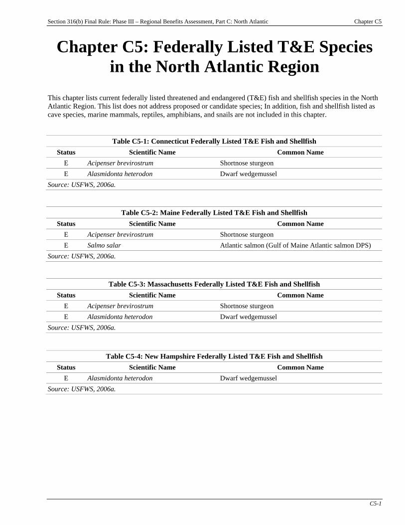
Section 316(b) Final Rule: Phase III – Regional Benefits Assessment, Part C: North Atlantic Chapter C5
C5-1
Chapter C5: Federally Listed T&E Species in the North Atlantic Region
This chapter lists current federally listed threatened and endangered (T&E) fish and shellfish species in the North Atlantic Region. This list does not address proposed or candidate species; In addition, fish and shellfish listed as cave species, marine mammals, reptiles, amphibians, and snails are not included in this chapter.
Table C5-1: Connecticut Federally Listed T&E Fish and Shellfish Status Scientific Name Common Name
E Acipenser brevirostrum Shortnose sturgeon E Alasmidonta heterodon Dwarf wedgemussel
Source: USFWS, 2006a.
Table C5-2: Maine Federally Listed T&E Fish and Shellfish Status Scientific Name Common Name
E Acipenser brevirostrum Shortnose sturgeon E Salmo salar Atlantic salmon (Gulf of Maine Atlantic salmon DPS)
Source: USFWS, 2006a.
Table C5-3: Massachusetts Federally Listed T&E Fish and Shellfish Status Scientific Name Common Name
E Acipenser brevirostrum Shortnose sturgeon E Alasmidonta heterodon Dwarf wedgemussel
Source: USFWS, 2006a.
Table C5-4: New Hampshire Federally Listed T&E Fish and Shellfish Status Scientific Name Common Name
E Alasmidonta heterodon Dwarf wedgemussel Source: USFWS, 2006a.

Section 316(b) Final Rule: Phase III – Regional Benefits Assessment
Part D: Mid-Atlantic Region

Section 316(b) Final Rule: Phase III – Regional Benefits Assessment, Part D: Mid-Atlantic Chapter D1
D1-1
Chapter D1: Background Introduction This chapter presents an overview of the potential Phase III existing facilities in the Mid-Atlantic study region and summarizes their key cooling water and compliance characteristics. For further discussion of the technical and compliance characteristics of potential Phase III existing facilities, refer to the Economic Analysis for the Final Section 316(b) Rule for Phase III Facilities and the Technical Development Document for the Final Section 316(b) Rule for Phase III Facilities (U.S. EPA, 2006a,c).
Chapter Contents D1-1 Facility Characteristics................................. D1-1
D1-1 Facility Characteristics The Mid-Atlantic Regional Study includes nine sample facilities that are potentially subject to the national standards for Phase III existing facilities. Figure D1-1 presents a map of these facilities. Five of them are manufacturing facilities and four are electric generators. Industry-wide, these nine sample facilities represent 15 facilities.PF
1FP
P
1P EPA applied sample weights to the survey respondents to account for non-sampled facilities and facilities that did
not respond to the survey. For more information on EPA’s 2000 Section 316(b) Industry Survey, please refer to the Information Collection Request (U.S. EPA, 2000b).
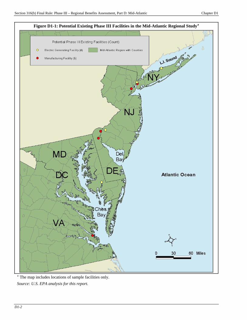
Section 316(b) Final Rule: Phase III – Regional Benefits Assessment, Part D: Mid-Atlantic Chapter D1
D1-2
Figure D1-1: Potential Existing Phase III Facilities in the Mid-Atlantic Regional StudyP
aP
P
aP The map includes locations of sample facilities only.
Source: U.S. EPA analysis for this report.
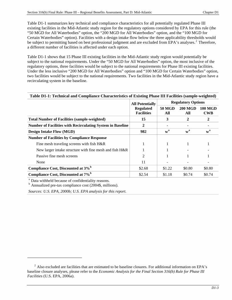
Section 316(b) Final Rule: Phase III – Regional Benefits Assessment, Part D: Mid-Atlantic Chapter D1
D1-3
Table D1-1 summarizes key technical and compliance characteristics for all potentially regulated Phase III existing facilities in the Mid-Atlantic study region for the regulatory options considered by EPA for this rule (the “50 MGD for All Waterbodies” option, the “200 MGD for All Waterbodies” option, and the “100 MGD for Certain Waterbodies” option). Facilities with a design intake flow below the three applicability thresholds would be subject to permitting based on best professional judgment and are excluded from EPA’s analyses.PF
2FP Therefore,
a different number of facilities is affected under each option. Table D1-1 shows that 15 Phase III existing facilities in the Mid-Atlantic study region would potentially be subject to the national requirements. Under the “50 MGD for All Waterbodies” option, the most inclusive of the regulatory options, three facilities would be subject to the national requirements for Phase III existing facilities. Under the less inclusive “200 MGD for All Waterbodies” option and “100 MGD for Certain Waterbodies” option, two facilities would be subject to the national requirements. Two facilities in the Mid-Atlantic study region have a recirculating system in the baseline.
Table D1-1: Technical and Compliance Characteristics of Existing Phase III Facilities (sample-weighted) Regulatory Options All Potentially
Regulated Facilities
50 MGD All
200 MGD All
100 MGD CWB
Total Number of Facilities (sample-weighted) 15 3 2 2 Number of Facilities with Recirculating System in Baseline 2 - - - Design Intake Flow (MGD) 982 wP
aP wP
aP wP
aP
Number of Facilities by Compliance Response Fine mesh traveling screens with fish H&R 1 1 1 1 New larger intake structure with fine mesh and fish H&R 1 1 - - Passive fine mesh screens 2 1 1 1 None 11 - - -
Compliance Cost, Discounted at 3%P
bP $2.68 $1.22 $0.80 $0.80
Compliance Cost, Discounted at 7%P
bP $2.54 $1.18 $0.74 $0.74
P
aP Data withheld because of confidentiality reasons.
P
bP Annualized pre-tax compliance cost (2004$, millions).
Sources: U.S. EPA, 2000b; U.S. EPA analysis for this report.
P
2P Also excluded are facilities that are estimated to be baseline closures. For additional information on EPA’s
baseline closure analyses, please refer to the Economic Analysis for the Final Section 316(b) Rule for Phase III Facilities (U.S. EPA, 2006a).
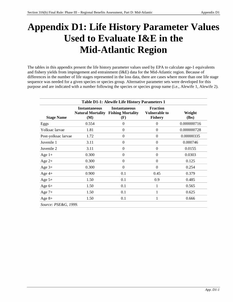
Section 316(b) Final Rule: Phase III – Regional Benefits Assessment, Part D: Mid-Atlantic Appendix D1
App. D1-1
Appendix D1: Life History Parameter Values Used to Evaluate I&E in the
Mid-Atlantic Region The tables in this appendix present the life history parameter values used by EPA to calculate age-1 equivalents and fishery yields from impingement and entrainment (I&E) data for the Mid-Atlantic region. Because of differences in the number of life stages represented in the loss data, there are cases where more than one life stage sequence was needed for a given species or species group. Alternative parameter sets were developed for this purpose and are indicated with a number following the species or species group name (i.e., Alewife 1, Alewife 2).
Table D1-1: Alewife Life History Parameters 1
Stage Name
Instantaneous Natural Mortality
(M)
Instantaneous Fishing Mortality
(F)
Fraction Vulnerable to
Fishery Weight
(lbs) Eggs 0.554 0 0 0.000000716 Yolksac larvae 1.81 0 0 0.000000728 Post-yolksac larvae 1.72 0 0 0.00000335 Juvenile 1 3.11 0 0 0.000746 Juvenile 2 3.11 0 0 0.0155 Age 1+ 0.300 0 0 0.0303 Age 2+ 0.300 0 0 0.125 Age 3+ 0.300 0 0 0.254 Age 4+ 0.900 0.1 0.45 0.379 Age 5+ 1.50 0.1 0.9 0.485 Age 6+ 1.50 0.1 1 0.565 Age 7+ 1.50 0.1 1 0.625 Age 8+ 1.50 0.1 1 0.666 Source: PSE&G, 1999.

Section 316(b) Final Rule: Phase III – Regional Benefits Assessment, Part D: Mid-Atlantic Appendix D1
App. D1-2
Table D1-2: Alewife Life History Parameters 2
Stage Name
Instantaneous Natural Mortality
(M)
Instantaneous Fishing Mortality
(F)
Fraction Vulnerable to
Fishery Weight
(lbs) Eggs 0.554 0 0 0.000000716 Larvae 3.53 0 0 0.00000204 Juvenile 6.21 0 0 0.000746 Age 1+ 0.300 0 0 0.0303 Age 2+ 0.300 0 0 0.125 Age 3+ 0.300 0 0 0.254 Age 4+ 0.900 0.1 0.45 0.379 Age 5+ 1.50 0.1 0.9 0.485 Age 6+ 1.50 0.1 1.0 0.565 Age 7+ 1.50 0.1 1.0 0.625 Age 8+ 1.50 0.1 1.0 0.666 Source: PSE&G, 1999.
Table D1-3: American Shad Life History Parameters
Stage Name
Instantaneous Natural Mortality
(M)
Instantaneous Fishing Mortality
(F)
Fraction Vulnerable to
Fishery Weight
(lbs) Eggs 0.496 0 0 0.000000716 Yolksac larvae 0.496 0 0 0.000000728 Post-yolksac larvae 2.52 0 0 0.00000335 Juvenile 7.4 0 0 0.000746 Age 1+ 0.3 0 0 0.309 Age 2+ 0.3 0 0 1.17 Age 3+ 0.3 0 0 2.32 Age 4+ 0.54 0.21 0.45 3.51 Age 5+ 1.02 0.21 0.90 4.56 Age 6+ 1.5 0.21 1.0 5.47 Age 7+ 1.5 0.21 1.0 6.20 Age 8+ 1.5 0.21 1.0 6.77 Sources: USFWS, 1978; Able and Fahay, 1998; PSE&G, 1999; and Froese and Pauly, 2001.
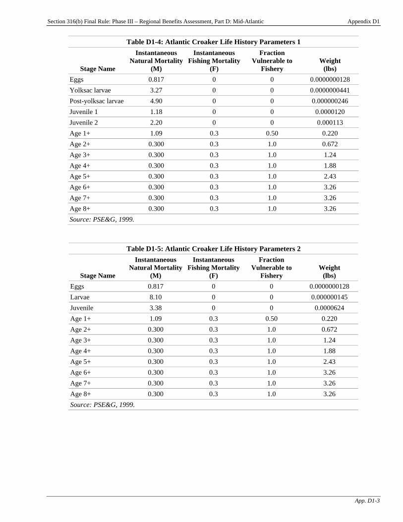
Section 316(b) Final Rule: Phase III – Regional Benefits Assessment, Part D: Mid-Atlantic Appendix D1
App. D1-3
Table D1-4: Atlantic Croaker Life History Parameters 1
Stage Name
Instantaneous Natural Mortality
(M)
Instantaneous Fishing Mortality
(F)
Fraction Vulnerable to
Fishery Weight
(lbs) Eggs 0.817 0 0 0.0000000128 Yolksac larvae 3.27 0 0 0.0000000441 Post-yolksac larvae 4.90 0 0 0.000000246 Juvenile 1 1.18 0 0 0.0000120 Juvenile 2 2.20 0 0 0.000113 Age 1+ 1.09 0.3 0.50 0.220 Age 2+ 0.300 0.3 1.0 0.672 Age 3+ 0.300 0.3 1.0 1.24 Age 4+ 0.300 0.3 1.0 1.88 Age 5+ 0.300 0.3 1.0 2.43 Age 6+ 0.300 0.3 1.0 3.26 Age 7+ 0.300 0.3 1.0 3.26 Age 8+ 0.300 0.3 1.0 3.26 Source: PSE&G, 1999.
Table D1-5: Atlantic Croaker Life History Parameters 2
Stage Name
Instantaneous Natural Mortality
(M)
Instantaneous Fishing Mortality
(F)
Fraction Vulnerable to
Fishery Weight
(lbs) Eggs 0.817 0 0 0.0000000128 Larvae 8.10 0 0 0.000000145 Juvenile 3.38 0 0 0.0000624 Age 1+ 1.09 0.3 0.50 0.220 Age 2+ 0.300 0.3 1.0 0.672 Age 3+ 0.300 0.3 1.0 1.24 Age 4+ 0.300 0.3 1.0 1.88 Age 5+ 0.300 0.3 1.0 2.43 Age 6+ 0.300 0.3 1.0 3.26 Age 7+ 0.300 0.3 1.0 3.26 Age 8+ 0.300 0.3 1.0 3.26 Source: PSE&G, 1999.
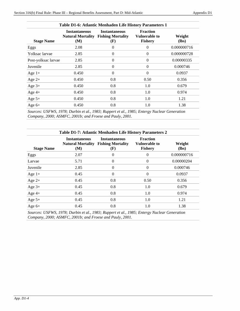
Section 316(b) Final Rule: Phase III – Regional Benefits Assessment, Part D: Mid-Atlantic Appendix D1
App. D1-4
Table D1-6: Atlantic Menhaden Life History Parameters 1
Stage Name
Instantaneous Natural Mortality
(M)
Instantaneous Fishing Mortality
(F)
Fraction Vulnerable to
Fishery Weight
(lbs) Eggs 2.08 0 0 0.000000716 Yolksac larvae 2.85 0 0 0.000000728 Post-yolksac larvae 2.85 0 0 0.00000335 Juvenile 2.85 0 0 0.000746 Age 1+ 0.450 0 0 0.0937 Age 2+ 0.450 0.8 0.50 0.356 Age 3+ 0.450 0.8 1.0 0.679 Age 4+ 0.450 0.8 1.0 0.974 Age 5+ 0.450 0.8 1.0 1.21 Age 6+ 0.450 0.8 1.0 1.38 Sources: USFWS, 1978; Durbin et al., 1983; Ruppert et al., 1985; Entergy Nuclear Generation Company, 2000; ASMFC, 2001b; and Froese and Pauly, 2001.
Table D1-7: Atlantic Menhaden Life History Parameters 2
Stage Name
Instantaneous Natural Mortality
(M)
Instantaneous Fishing Mortality
(F)
Fraction Vulnerable to
Fishery Weight
(lbs) Eggs 2.07 0 0 0.000000716 Larvae 5.71 0 0 0.00000204 Juvenile 2.85 0 0 0.000746 Age 1+ 0.45 0 0 0.0937 Age 2+ 0.45 0.8 0.50 0.356 Age 3+ 0.45 0.8 1.0 0.679 Age 4+ 0.45 0.8 1.0 0.974 Age 5+ 0.45 0.8 1.0 1.21 Age 6+ 0.45 0.8 1.0 1.38 Sources: USFWS, 1978; Durbin et al., 1983; Ruppert et al., 1985; Entergy Nuclear Generation Company, 2000; ASMFC, 2001b; and Froese and Pauly, 2001.
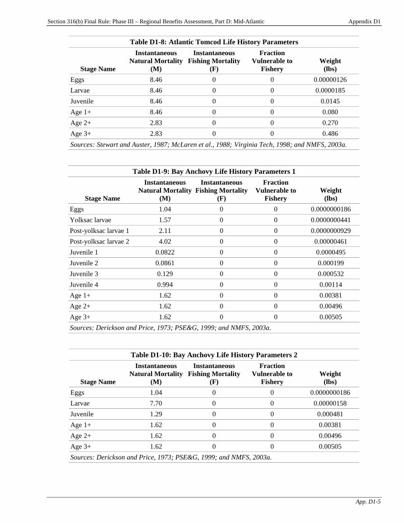
Section 316(b) Final Rule: Phase III – Regional Benefits Assessment, Part D: Mid-Atlantic Appendix D1
App. D1-5
Table D1-8: Atlantic Tomcod Life History Parameters
Stage Name
Instantaneous Natural Mortality
(M)
Instantaneous Fishing Mortality
(F)
Fraction Vulnerable to
Fishery Weight
(lbs) Eggs 8.46 0 0 0.00000126 Larvae 8.46 0 0 0.0000185 Juvenile 8.46 0 0 0.0145 Age 1+ 8.46 0 0 0.080 Age 2+ 2.83 0 0 0.270 Age 3+ 2.83 0 0 0.486 Sources: TStewart and Auster, 1987; McLaren et al., 1988;T Virginia Tech, 1998; and NMFS, 2003a.
Table D1-9: Bay Anchovy Life History Parameters 1
Stage Name
Instantaneous Natural Mortality
(M)
Instantaneous Fishing Mortality
(F)
Fraction Vulnerable to
Fishery Weight
(lbs) Eggs 1.04 0 0 0.0000000186 Yolksac larvae 1.57 0 0 0.0000000441 Post-yolksac larvae 1 2.11 0 0 0.0000000929 Post-yolksac larvae 2 4.02 0 0 0.00000461 Juvenile 1 0.0822 0 0 0.0000495 Juvenile 2 0.0861 0 0 0.000199 Juvenile 3 0.129 0 0 0.000532 Juvenile 4 0.994 0 0 0.00114 Age 1+ 1.62 0 0 0.00381 Age 2+ 1.62 0 0 0.00496 Age 3+ 1.62 0 0 0.00505 Sources: Derickson and Price, 1973; PSE&G, 1999; and NMFS, 2003a.
Table D1-10: Bay Anchovy Life History Parameters 2
Stage Name
Instantaneous Natural Mortality
(M)
Instantaneous Fishing Mortality
(F)
Fraction Vulnerable to
Fishery Weight
(lbs) Eggs 1.04 0 0 0.0000000186 Larvae 7.70 0 0 0.00000158 Juvenile 1.29 0 0 0.000481 Age 1+ 1.62 0 0 0.00381 Age 2+ 1.62 0 0 0.00496 Age 3+ 1.62 0 0 0.00505 Sources: Derickson and Price, 1973; PSE&G, 1999; and NMFS, 2003a.
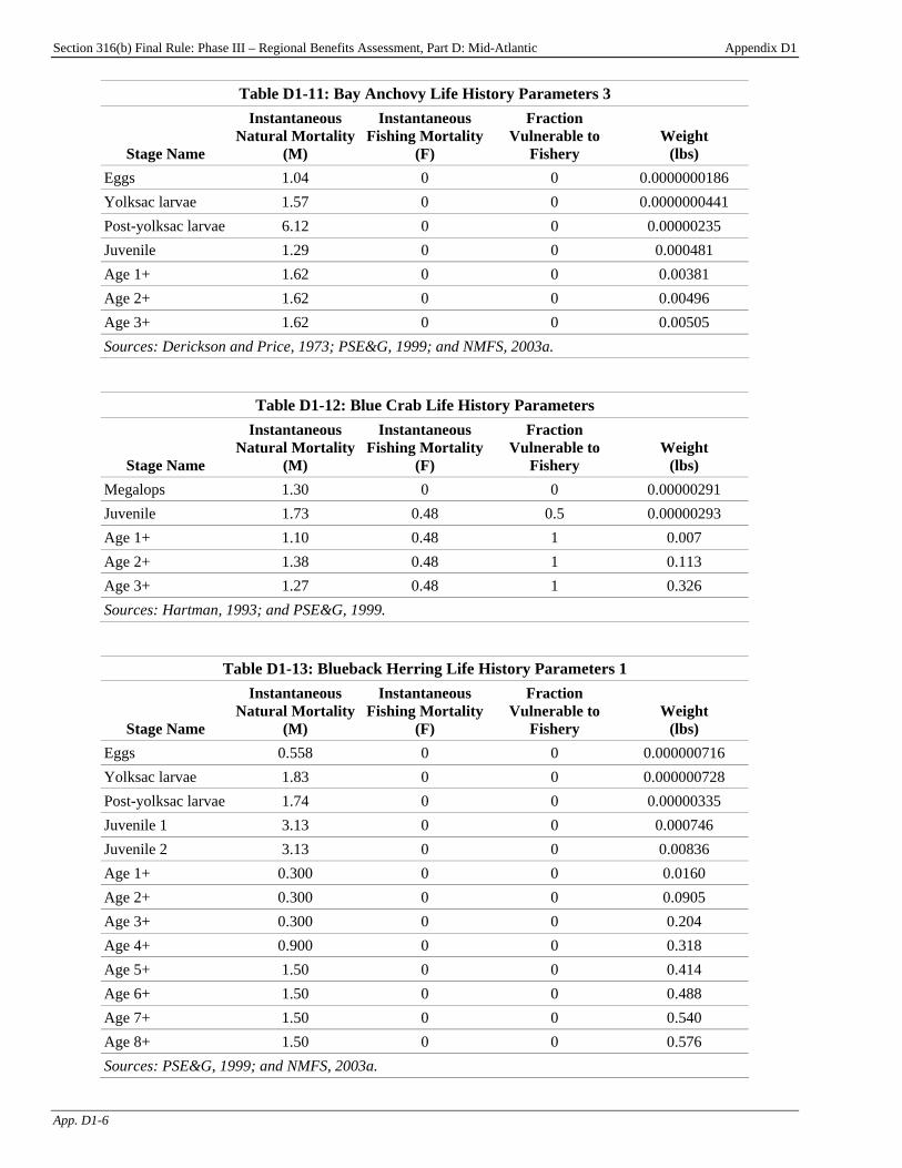
Section 316(b) Final Rule: Phase III – Regional Benefits Assessment, Part D: Mid-Atlantic Appendix D1
App. D1-6
Table D1-11: Bay Anchovy Life History Parameters 3
Stage Name
Instantaneous Natural Mortality
(M)
Instantaneous Fishing Mortality
(F)
Fraction Vulnerable to
Fishery Weight
(lbs) Eggs 1.04 0 0 0.0000000186 Yolksac larvae 1.57 0 0 0.0000000441 Post-yolksac larvae 6.12 0 0 0.00000235 Juvenile 1.29 0 0 0.000481 Age 1+ 1.62 0 0 0.00381 Age 2+ 1.62 0 0 0.00496 Age 3+ 1.62 0 0 0.00505 Sources: Derickson and Price, 1973; PSE&G, 1999; and NMFS, 2003a.
Table D1-12: Blue Crab Life History Parameters
Stage Name
Instantaneous Natural Mortality
(M)
Instantaneous Fishing Mortality
(F)
Fraction Vulnerable to
Fishery Weight
(lbs) Megalops 1.30 0 0 0.00000291 Juvenile 1.73 0.48 0.5 0.00000293 Age 1+ 1.10 0.48 1 0.007 Age 2+ 1.38 0.48 1 0.113 Age 3+ 1.27 0.48 1 0.326 Sources: Hartman, 1993; and PSE&G, 1999.
Table D1-13: Blueback Herring Life History Parameters 1
Stage Name
Instantaneous Natural Mortality
(M)
Instantaneous Fishing Mortality
(F)
Fraction Vulnerable to
Fishery Weight
(lbs) Eggs 0.558 0 0 0.000000716 Yolksac larvae 1.83 0 0 0.000000728 Post-yolksac larvae 1.74 0 0 0.00000335 Juvenile 1 3.13 0 0 0.000746 Juvenile 2 3.13 0 0 0.00836 Age 1+ 0.300 0 0 0.0160 Age 2+ 0.300 0 0 0.0905 Age 3+ 0.300 0 0 0.204 Age 4+ 0.900 0 0 0.318 Age 5+ 1.50 0 0 0.414 Age 6+ 1.50 0 0 0.488 Age 7+ 1.50 0 0 0.540 Age 8+ 1.50 0 0 0.576 Sources: PSE&G, 1999; and NMFS, 2003a.
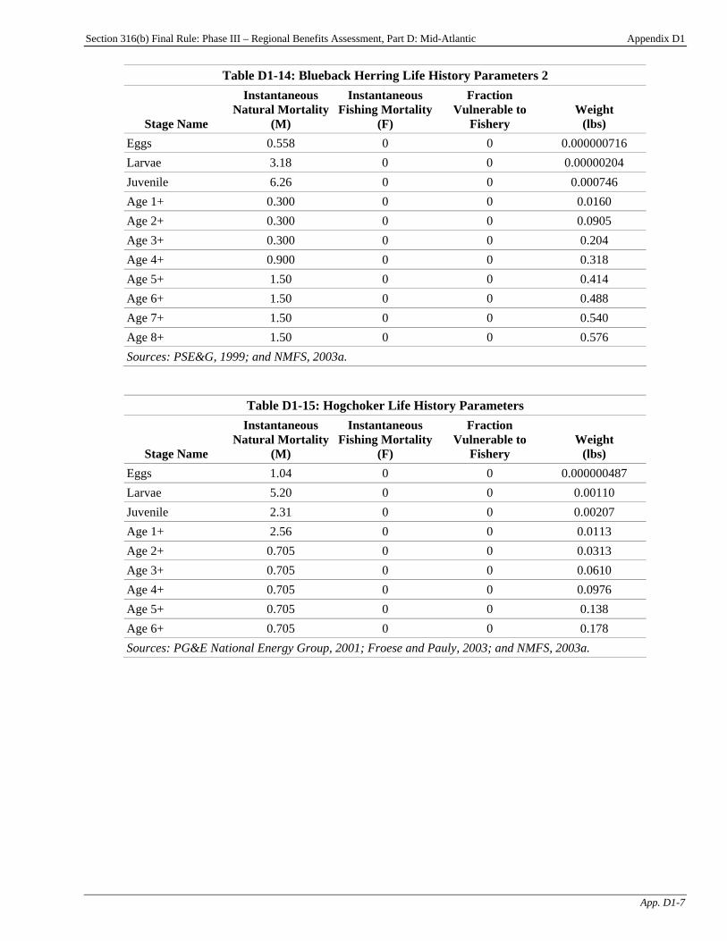
Section 316(b) Final Rule: Phase III – Regional Benefits Assessment, Part D: Mid-Atlantic Appendix D1
App. D1-7
Table D1-14: Blueback Herring Life History Parameters 2
Stage Name
Instantaneous Natural Mortality
(M)
Instantaneous Fishing Mortality
(F)
Fraction Vulnerable to
Fishery Weight
(lbs) Eggs 0.558 0 0 0.000000716 Larvae 3.18 0 0 0.00000204 Juvenile 6.26 0 0 0.000746 Age 1+ 0.300 0 0 0.0160 Age 2+ 0.300 0 0 0.0905 Age 3+ 0.300 0 0 0.204 Age 4+ 0.900 0 0 0.318 Age 5+ 1.50 0 0 0.414 Age 6+ 1.50 0 0 0.488 Age 7+ 1.50 0 0 0.540 Age 8+ 1.50 0 0 0.576 Sources: PSE&G, 1999; and NMFS, 2003a.
Table D1-15: Hogchoker Life History Parameters
Stage Name
Instantaneous Natural Mortality
(M)
Instantaneous Fishing Mortality
(F)
Fraction Vulnerable to
Fishery Weight
(lbs) Eggs 1.04 0 0 0.000000487 Larvae 5.20 0 0 0.00110 Juvenile 2.31 0 0 0.00207 Age 1+ 2.56 0 0 0.0113 Age 2+ 0.705 0 0 0.0313 Age 3+ 0.705 0 0 0.0610 Age 4+ 0.705 0 0 0.0976 Age 5+ 0.705 0 0 0.138 Age 6+ 0.705 0 0 0.178 Sources: PG&E National Energy Group, 2001; Froese and Pauly, 2003; and NMFS, 2003a.
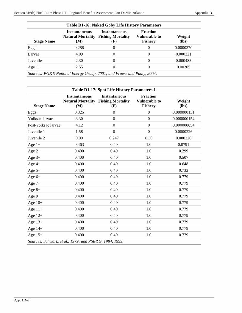
Section 316(b) Final Rule: Phase III – Regional Benefits Assessment, Part D: Mid-Atlantic Appendix D1
App. D1-8
Table D1-16: Naked Goby Life History Parameters
Stage Name
Instantaneous Natural Mortality
(M)
Instantaneous Fishing Mortality
(F)
Fraction Vulnerable to
Fishery Weight
(lbs) Eggs 0.288 0 0 0.0000370 Larvae 4.09 0 0 0.000221 Juvenile 2.30 0 0 0.000485 Age 1+ 2.55 0 0 0.00205 Sources: TPG&E National Energy Group, 2001; and Froese and Pauly, 2003T.
Table D1-17: Spot Life History Parameters 1
Stage Name
Instantaneous Natural Mortality
(M)
Instantaneous Fishing Mortality
(F)
Fraction Vulnerable to
Fishery Weight
(lbs) Eggs 0.825 0 0 0.000000131 Yolksac larvae 3.30 0 0 0.000000154 Post-yolksac larvae 4.12 0 0 0.000000854 Juvenile 1 1.58 0 0 0.0000226 Juvenile 2 0.99 0.247 0.30 0.000220 Age 1+ 0.463 0.40 1.0 0.0791 Age 2+ 0.400 0.40 1.0 0.299 Age 3+ 0.400 0.40 1.0 0.507 Age 4+ 0.400 0.40 1.0 0.648 Age 5+ 0.400 0.40 1.0 0.732 Age 6+ 0.400 0.40 1.0 0.779 Age 7+ 0.400 0.40 1.0 0.779 Age 8+ 0.400 0.40 1.0 0.779 Age 9+ 0.400 0.40 1.0 0.779 Age 10+ 0.400 0.40 1.0 0.779 Age 11+ 0.400 0.40 1.0 0.779 Age 12+ 0.400 0.40 1.0 0.779 Age 13+ 0.400 0.40 1.0 0.779 Age 14+ 0.400 0.40 1.0 0.779 Age 15+ 0.400 0.40 1.0 0.779 Sources: Schwartz et al., 1979; and PSE&G, 1984, 1999.

Section 316(b) Final Rule: Phase III – Regional Benefits Assessment, Part D: Mid-Atlantic Appendix D1
App. D1-9
Table D1-18: Spot Life History Parameters 2
Stage Name
Instantaneous Natural Mortality
(M)
Instantaneous Fishing Mortality
(F)
Fraction Vulnerable to
Fishery Weight
(lbs) Eggs 0.825 0 0 0.000000131 Larvae 7.40 0 0 0.000000504 Juvenile 2.57 0 0 0.000121 Age 1+ 0.463 0.40 1.0 0.0791 Age 2+ 0.400 0.40 1.0 0.299 Age 3+ 0.400 0.40 1.0 0.507 Age 4+ 0.400 0.40 1.0 0.648 Age 5+ 0.400 0.40 1.0 0.732 Age 6+ 0.400 0.40 1.0 0.779 Age 7+ 0.400 0.40 1.0 0.779 Age 8+ 0.400 0.40 1.0 0.779 Age 9+ 0.400 0.40 1.0 0.779 Age 10+ 0.400 0.40 1.0 0.779 Age 11+ 0.400 0.40 1.0 0.779 Age 12+ 0.400 0.40 1.0 0.779 Age 13+ 0.400 0.40 1.0 0.779 Age 14+ 0.400 0.40 1.0 0.779 Age 15+ 0.400 0.40 1.0 0.779 Sources: Schwartz et al., 1979; and PSE&G, 1984, 1999.

Section 316(b) Final Rule: Phase III – Regional Benefits Assessment, Part D: Mid-Atlantic Appendix D1
App. D1-10
Table D1-19: Striped Bass Life History Parameters 1
Stage Name
Instantaneous Natural Mortality
(M)
Instantaneous Fishing Mortality
(F)
Fraction Vulnerable to
Fishery Weight
(lbs) Eggs 1.39 0 0 0.000000224 Yolksac larvae 2.22 0 0 0.000000243 Post-yolksac larvae 5.11 0 0 0.0000119 Juvenile 1 2.28 0 0 0.000154 Juvenile 2 1.00 0 0 0.0216 Age 1+ 1.10 0 0 0.485 Age 2+ 0.150 0.31 0.06 2.06 Age 3+ 0.150 0.31 0.20 3.31 Age 4+ 0.150 0.31 0.63 4.93 Age 5+ 0.150 0.31 0.94 6.50 Age 6+ 0.150 0.31 1.0 8.58 Age 7+ 0.150 0.31 0.90 12.3 Age 8+ 0.150 0.31 0.90 14.3 Age 9+ 0.150 0.31 0.90 16.1 Age 10+ 0.150 0.31 0.90 18.8 Age 11+ 0.150 0.31 0.90 19.6 Age 12+ 0.150 0.31 0.90 22.4 Age 13+ 0.150 0.31 0.90 27.0 Age 14+ 0.150 0.31 0.90 34.6 Age 15+ 0.150 0.31 0.90 41.5 Sources: Bason, 1971; and PSE&G, 1999.
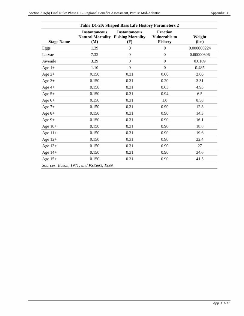
Section 316(b) Final Rule: Phase III – Regional Benefits Assessment, Part D: Mid-Atlantic Appendix D1
App. D1-11
Table D1-20: Striped Bass Life History Parameters 2
Stage Name
Instantaneous Natural Mortality
(M)
Instantaneous Fishing Mortality
(F)
Fraction Vulnerable to
Fishery Weight
(lbs) Eggs 1.39 0 0 0.000000224 Larvae 7.32 0 0 0.00000606 Juvenile 3.29 0 0 0.0109 Age 1+ 1.10 0 0 0.485 Age 2+ 0.150 0.31 0.06 2.06 Age 3+ 0.150 0.31 0.20 3.31 Age 4+ 0.150 0.31 0.63 4.93 Age 5+ 0.150 0.31 0.94 6.5 Age 6+ 0.150 0.31 1.0 8.58 Age 7+ 0.150 0.31 0.90 12.3 Age 8+ 0.150 0.31 0.90 14.3 Age 9+ 0.150 0.31 0.90 16.1 Age 10+ 0.150 0.31 0.90 18.8 Age 11+ 0.150 0.31 0.90 19.6 Age 12+ 0.150 0.31 0.90 22.4 Age 13+ 0.150 0.31 0.90 27 Age 14+ 0.150 0.31 0.90 34.6 Age 15+ 0.150 0.31 0.90 41.5 Sources: Bason, 1971; and PSE&G, 1999.
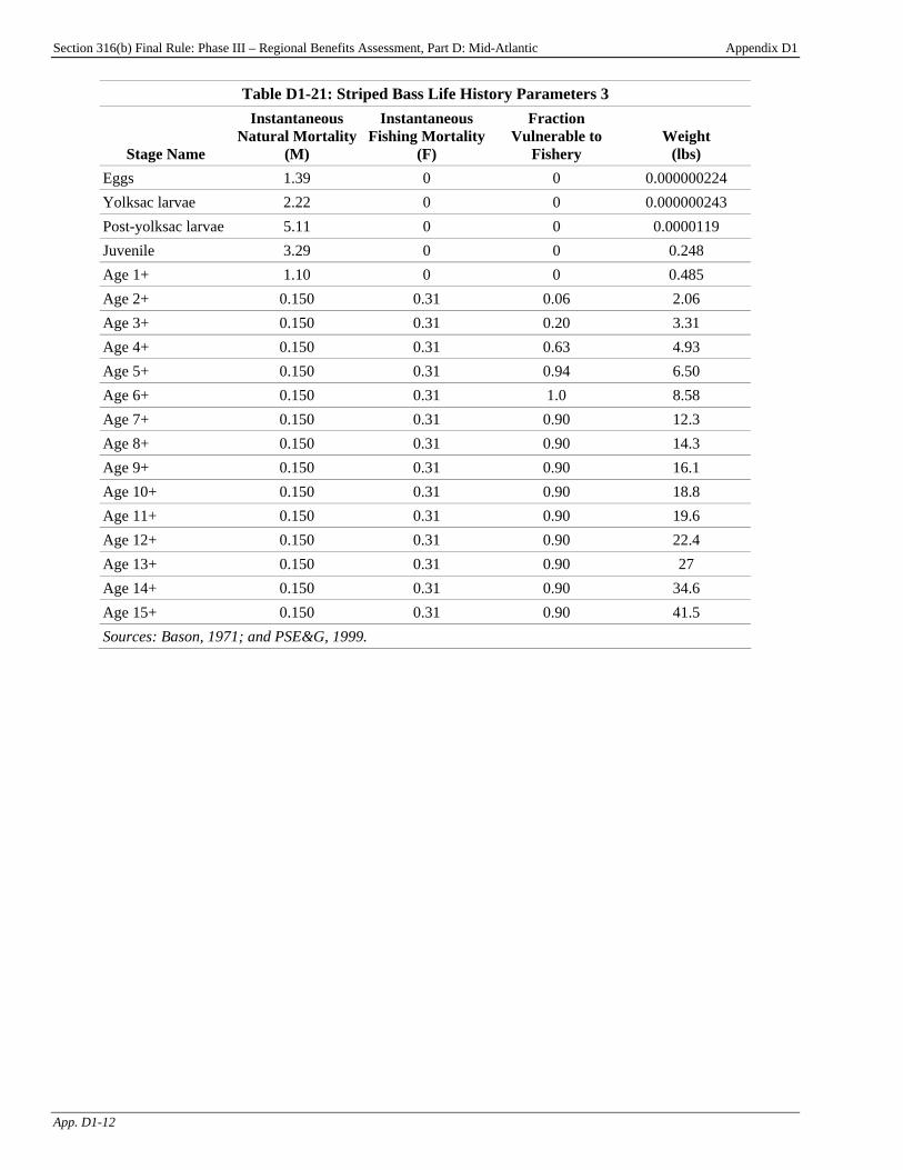
Section 316(b) Final Rule: Phase III – Regional Benefits Assessment, Part D: Mid-Atlantic Appendix D1
App. D1-12
Table D1-21: Striped Bass Life History Parameters 3
Stage Name
Instantaneous Natural Mortality
(M)
Instantaneous Fishing Mortality
(F)
Fraction Vulnerable to
Fishery Weight
(lbs) Eggs 1.39 0 0 0.000000224 Yolksac larvae 2.22 0 0 0.000000243 Post-yolksac larvae 5.11 0 0 0.0000119 Juvenile 3.29 0 0 0.248 Age 1+ 1.10 0 0 0.485 Age 2+ 0.150 0.31 0.06 2.06 Age 3+ 0.150 0.31 0.20 3.31 Age 4+ 0.150 0.31 0.63 4.93 Age 5+ 0.150 0.31 0.94 6.50 Age 6+ 0.150 0.31 1.0 8.58 Age 7+ 0.150 0.31 0.90 12.3 Age 8+ 0.150 0.31 0.90 14.3 Age 9+ 0.150 0.31 0.90 16.1 Age 10+ 0.150 0.31 0.90 18.8 Age 11+ 0.150 0.31 0.90 19.6 Age 12+ 0.150 0.31 0.90 22.4 Age 13+ 0.150 0.31 0.90 27 Age 14+ 0.150 0.31 0.90 34.6 Age 15+ 0.150 0.31 0.90 41.5 Sources: Bason, 1971; and PSE&G, 1999.
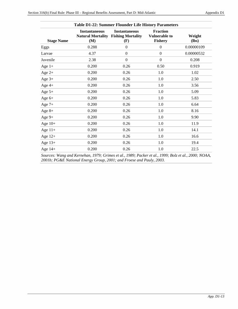
Section 316(b) Final Rule: Phase III – Regional Benefits Assessment, Part D: Mid-Atlantic Appendix D1
App. D1-13
Table D1-22: Summer Flounder Life History Parameters
Stage Name
Instantaneous Natural Mortality
(M)
Instantaneous Fishing Mortality
(F)
Fraction Vulnerable to
Fishery Weight
(lbs) Eggs 0.288 0 0 0.00000109 Larvae 4.37 0 0 0.00000532 Juvenile 2.38 0 0 0.208 Age 1+ 0.200 0.26 0.50 0.919 Age 2+ 0.200 0.26 1.0 1.02 Age 3+ 0.200 0.26 1.0 2.50 Age 4+ 0.200 0.26 1.0 3.56 Age 5+ 0.200 0.26 1.0 5.09 Age 6+ 0.200 0.26 1.0 5.83 Age 7+ 0.200 0.26 1.0 6.64 Age 8+ 0.200 0.26 1.0 8.16 Age 9+ 0.200 0.26 1.0 9.90 Age 10+ 0.200 0.26 1.0 11.9 Age 11+ 0.200 0.26 1.0 14.1 Age 12+ 0.200 0.26 1.0 16.6 Age 13+ 0.200 0.26 1.0 19.4 Age 14+ 0.200 0.26 1.0 22.5 Sources: Wang and Kernehan, 1979; Grimes et al., 1989; Packer et al., 1999; Bolz et al., 2000; NOAA, 2001b; PG&E National Energy Group, 2001; and Froese and Pauly, 2003.
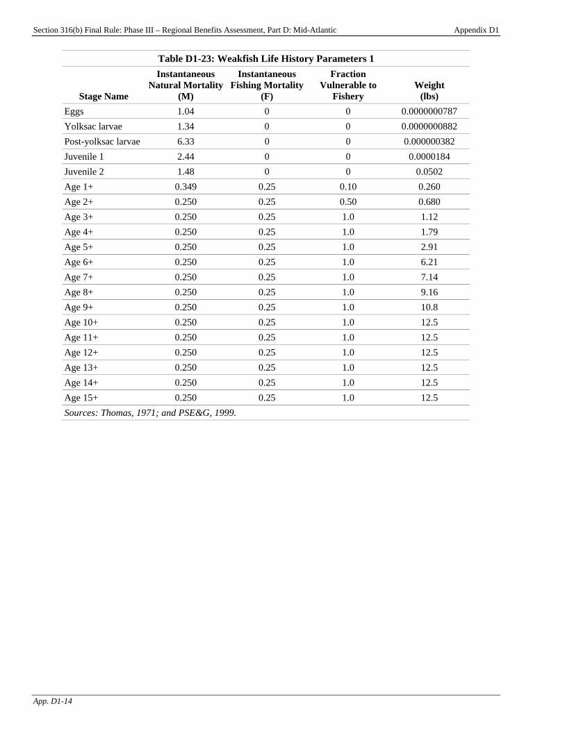
Section 316(b) Final Rule: Phase III – Regional Benefits Assessment, Part D: Mid-Atlantic Appendix D1
App. D1-14
Table D1-23: Weakfish Life History Parameters 1
Stage Name
Instantaneous Natural Mortality
(M)
Instantaneous Fishing Mortality
(F)
Fraction Vulnerable to
Fishery Weight
(lbs) Eggs 1.04 0 0 0.0000000787 Yolksac larvae 1.34 0 0 0.0000000882 Post-yolksac larvae 6.33 0 0 0.000000382 Juvenile 1 2.44 0 0 0.0000184 Juvenile 2 1.48 0 0 0.0502 Age 1+ 0.349 0.25 0.10 0.260 Age 2+ 0.250 0.25 0.50 0.680 Age 3+ 0.250 0.25 1.0 1.12 Age 4+ 0.250 0.25 1.0 1.79 Age 5+ 0.250 0.25 1.0 2.91 Age 6+ 0.250 0.25 1.0 6.21 Age 7+ 0.250 0.25 1.0 7.14 Age 8+ 0.250 0.25 1.0 9.16 Age 9+ 0.250 0.25 1.0 10.8 Age 10+ 0.250 0.25 1.0 12.5 Age 11+ 0.250 0.25 1.0 12.5 Age 12+ 0.250 0.25 1.0 12.5 Age 13+ 0.250 0.25 1.0 12.5 Age 14+ 0.250 0.25 1.0 12.5 Age 15+ 0.250 0.25 1.0 12.5 Sources: Thomas, 1971; and PSE&G, 1999.
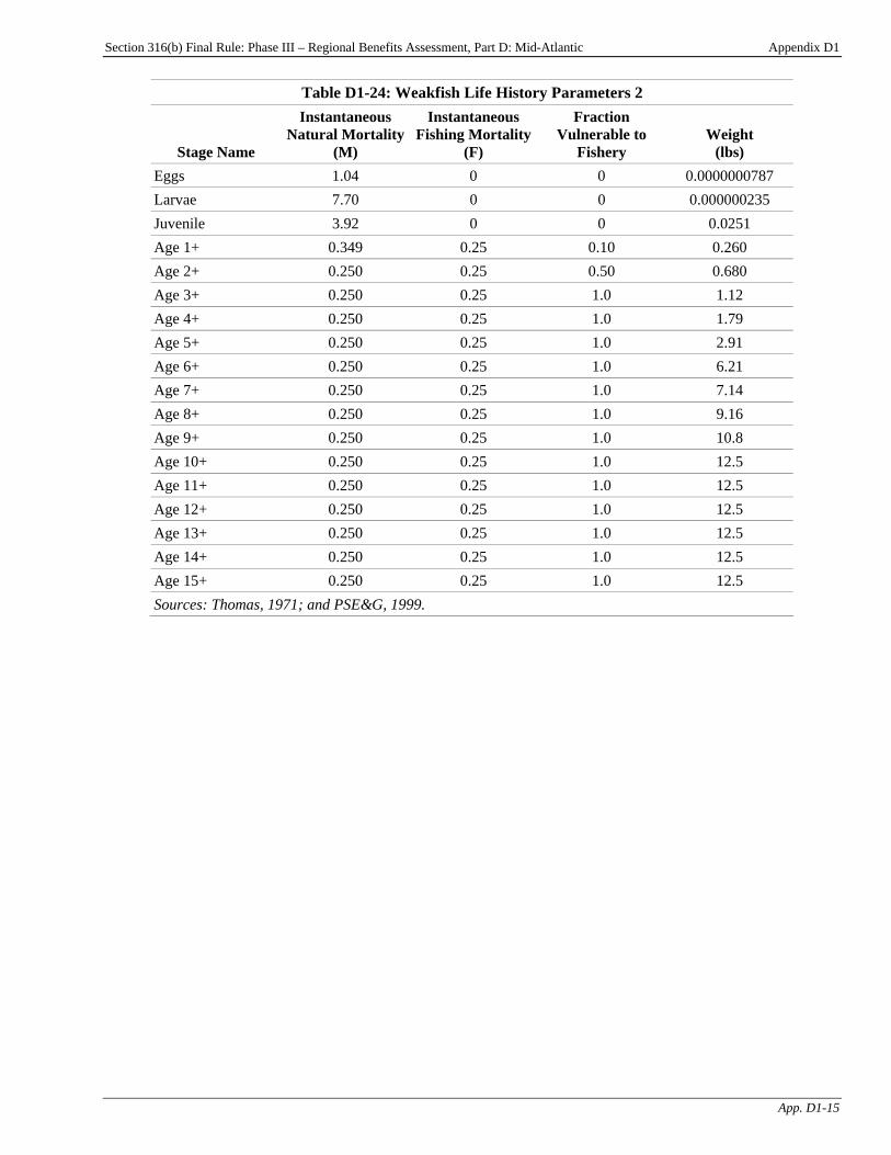
Section 316(b) Final Rule: Phase III – Regional Benefits Assessment, Part D: Mid-Atlantic Appendix D1
App. D1-15
Table D1-24: Weakfish Life History Parameters 2
Stage Name
Instantaneous Natural Mortality
(M)
Instantaneous Fishing Mortality
(F)
Fraction Vulnerable to
Fishery Weight
(lbs) Eggs 1.04 0 0 0.0000000787 Larvae 7.70 0 0 0.000000235 Juvenile 3.92 0 0 0.0251 Age 1+ 0.349 0.25 0.10 0.260 Age 2+ 0.250 0.25 0.50 0.680 Age 3+ 0.250 0.25 1.0 1.12 Age 4+ 0.250 0.25 1.0 1.79 Age 5+ 0.250 0.25 1.0 2.91 Age 6+ 0.250 0.25 1.0 6.21 Age 7+ 0.250 0.25 1.0 7.14 Age 8+ 0.250 0.25 1.0 9.16 Age 9+ 0.250 0.25 1.0 10.8 Age 10+ 0.250 0.25 1.0 12.5 Age 11+ 0.250 0.25 1.0 12.5 Age 12+ 0.250 0.25 1.0 12.5 Age 13+ 0.250 0.25 1.0 12.5 Age 14+ 0.250 0.25 1.0 12.5 Age 15+ 0.250 0.25 1.0 12.5 Sources: Thomas, 1971; and PSE&G, 1999.
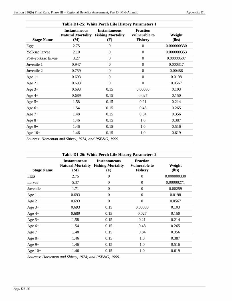
Section 316(b) Final Rule: Phase III – Regional Benefits Assessment, Part D: Mid-Atlantic Appendix D1
App. D1-16
Table D1-25: White Perch Life History Parameters 1
Stage Name
Instantaneous Natural Mortality
(M)
Instantaneous Fishing Mortality
(F)
Fraction Vulnerable to
Fishery Weight
(lbs) Eggs 2.75 0 0 0.000000330 Yolksac larvae 2.10 0 0 0.000000353 Post-yolksac larvae 3.27 0 0 0.00000507 Juvenile 1 0.947 0 0 0.000317 Juvenile 2 0.759 0 0 0.00486 Age 1+ 0.693 0 0 0.0198 Age 2+ 0.693 0 0 0.0567 Age 3+ 0.693 0.15 0.00080 0.103 Age 4+ 0.689 0.15 0.027 0.150 Age 5+ 1.58 0.15 0.21 0.214 Age 6+ 1.54 0.15 0.48 0.265 Age 7+ 1.48 0.15 0.84 0.356 Age 8+ 1.46 0.15 1.0 0.387 Age 9+ 1.46 0.15 1.0 0.516 Age 10+ 1.46 0.15 1.0 0.619 Sources: Horseman and Shirey, 1974; and PSE&G, 1999.
Table D1-26: White Perch Life History Parameters 2
Stage Name
Instantaneous Natural Mortality
(M)
Instantaneous Fishing Mortality
(F)
Fraction Vulnerable to
Fishery Weight
(lbs) Eggs 2.75 0 0 0.000000330 Larvae 5.37 0 0 0.00000271 Juvenile 1.71 0 0 0.00259 Age 1+ 0.693 0 0 0.0198 Age 2+ 0.693 0 0 0.0567 Age 3+ 0.693 0.15 0.00080 0.103 Age 4+ 0.689 0.15 0.027 0.150 Age 5+ 1.58 0.15 0.21 0.214 Age 6+ 1.54 0.15 0.48 0.265 Age 7+ 1.48 0.15 0.84 0.356 Age 8+ 1.46 0.15 1.0 0.387 Age 9+ 1.46 0.15 1.0 0.516 Age 10+ 1.46 0.15 1.0 0.619 Sources: Horseman and Shirey, 1974; and PSE&G, 1999.

Section 316(b) Final Rule: Phase III – Regional Benefits Assessment, Part D: Mid-Atlantic Appendix D1
App. D1-17
Table D1-27: White Perch Life History Parameters 3
Stage Name
Instantaneous Natural Mortality
(M)
Instantaneous Fishing Mortality
(F)
Fraction Vulnerable to
Fishery Weight
(lbs) Eggs 2.75 0 0 0.000000330 Yolksac larvae 2.10 0 0 0.000000353 Post-yolksac larvae 3.27 0 0 0.00000507 Juvenile 1.71 0 0 0.00259 Age 1+ 0.693 0 0 0.0198 Age 2+ 0.693 0 0 0.0567 Age 3+ 0.693 0.15 0.00080 0.103 Age 4+ 0.689 0.15 0.027 0.150 Age 5+ 1.58 0.15 0.21 0.214 Age 6+ 1.54 0.15 0.48 0.265 Age 7+ 1.48 0.15 0.84 0.356 Age 8+ 1.46 0.15 1.0 0.387 Age 9+ 1.46 0.15 1.0 0.516 Age 10+ 1.46 0.15 1.0 0.619 Sources: Horseman and Shirey, 1974; and PSE&G, 1999.
Table D1-28: Windowpane Life History Parameters
Stage Name
Instantaneous Natural Mortality
(M)
Instantaneous Fishing Mortality
(F)
Fraction Vulnerable to
Fishery Weight
(lbs) Eggs 1.41 0 0 0.00000154 Larvae 6.99 0 0 0.00165 Juvenile 2.98 0 0 0.00223 Age 1+ 0.420 0 0 0.0325 Age 2+ 0.420 1.6 0.25 0.122 Age 3+ 0.420 1.6 0.61 0.265 Age 4+ 0.420 1.6 1.0 0.433 Age 5+ 0.420 1.6 1.0 0.603 Age 6+ 0.420 1.6 1.0 0.761 Age 7+ 0.420 1.6 1.0 0.899 Age 8+ 0.420 1.6 1.0 1.02 Age 9+ 0.420 1.6 1.0 1.11 Age 10+ 0.420 1.6 1.0 1.19 Sources: Hendrickson, 2000; PG&E National Energy Group, 2001; USGen New England, 2001; and Froese and Pauly, 2003.

Section 316(b) Final Rule: Phase III – Regional Benefits Assessment, Part D: Mid-Atlantic Appendix D1
App. D1-18
Table D1-29: Winter Flounder Life History Parameters
Stage Name
Instantaneous Natural Mortality
(M)
Instantaneous Fishing Mortality
(F)
Fraction Vulnerable to
Fishery Weight
(lbs) Eggs 0.288 0 0 0.00000115 Larvae 4.37 0 0 0.0138 Juvenile 2.38 0 0 0.0330 Age 1+ 1.10 0.24 0.01 0.208 Age 2+ 0.924 0.24 0.29 0.562 Age 3+ 0.200 0.24 0.80 0.997 Age 4+ 0.200 0.24 0.92 1.42 Age 5+ 0.200 0.24 0.83 1.78 Age 6+ 0.200 0.24 0.89 2.07 Age 7+ 0.200 0.24 0.89 2.29 Age 8+ 0.200 0.24 0.89 2.45 Age 9+ 0.200 0.24 0.89 2.57 Age 10+ 0.200 0.24 0.89 2.65 Age 11+ 0.200 0.24 0.89 2.71 Age 12+ 0.200 0.24 0.89 2.75 Age 13+ 0.200 0.24 0.89 2.78 Age 14+ 0.200 0.24 0.89 2.80 Age 15+ 0.200 0.24 0.89 2.82 Age 16+ 0.200 0.24 0.89 2.83 Sources: Able and Fahay, 1998; Colarusso, 2000; Nitschke et al., 2000; and PG&E National Energy Group, 2001.
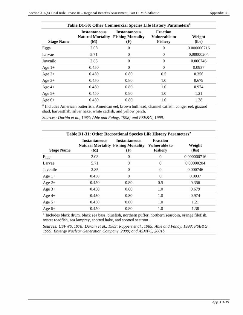
Section 316(b) Final Rule: Phase III – Regional Benefits Assessment, Part D: Mid-Atlantic Appendix D1
App. D1-19
Table D1-30: Other Commercial Species Life History ParametersP
aP
Stage Name
Instantaneous Natural Mortality
(M)
Instantaneous Fishing Mortality
(F)
Fraction Vulnerable to
Fishery Weight
(lbs) Eggs 2.08 0 0 0.000000716 Larvae 5.71 0 0 0.00000204 Juvenile 2.85 0 0 0.000746 Age 1+ 0.450 0 0 0.0937 Age 2+ 0.450 0.80 0.5 0.356 Age 3+ 0.450 0.80 1.0 0.679 Age 4+ 0.450 0.80 1.0 0.974 Age 5+ 0.450 0.80 1.0 1.21 Age 6+ 0.450 0.80 1.0 1.38 P
aP Includes American butterfish, American eel, brown bullhead, channel catfish, conger eel, gizzard
shad, harvestfish, silver hake, white catfish, and yellow perch. Sources: Durbin et al., 1983; Able and Fahay, 1998; and PSE&G, 1999.
Table D1-31: Other Recreational Species Life History ParametersP
aP
Stage Name
Instantaneous Natural Mortality
(M)
Instantaneous Fishing Mortality
(F)
Fraction Vulnerable to
Fishery Weight
(lbs) Eggs 2.08 0 0 0.000000716 Larvae 5.71 0 0 0.00000204 Juvenile 2.85 0 0 0.000746 Age 1+ 0.450 0 0 0.0937 Age 2+ 0.450 0.80 0.5 0.356 Age 3+ 0.450 0.80 1.0 0.679 Age 4+ 0.450 0.80 1.0 0.974 Age 5+ 0.450 0.80 1.0 1.21 Age 6+ 0.450 0.80 1.0 1.38 P
aP Includes black drum, black sea bass, bluefish, northern puffer, northern searobin, orange filefish,
oyster toadfish, sea lamprey, spotted hake, and spotted seatrout. Sources: USFWS, 1978; Durbin et al., 1983; Ruppert et al., 1985; Able and Fahay, 1998; PSE&G, 1999; Entergy Nuclear Generation Company, 2000; and ASMFC, 2001b.
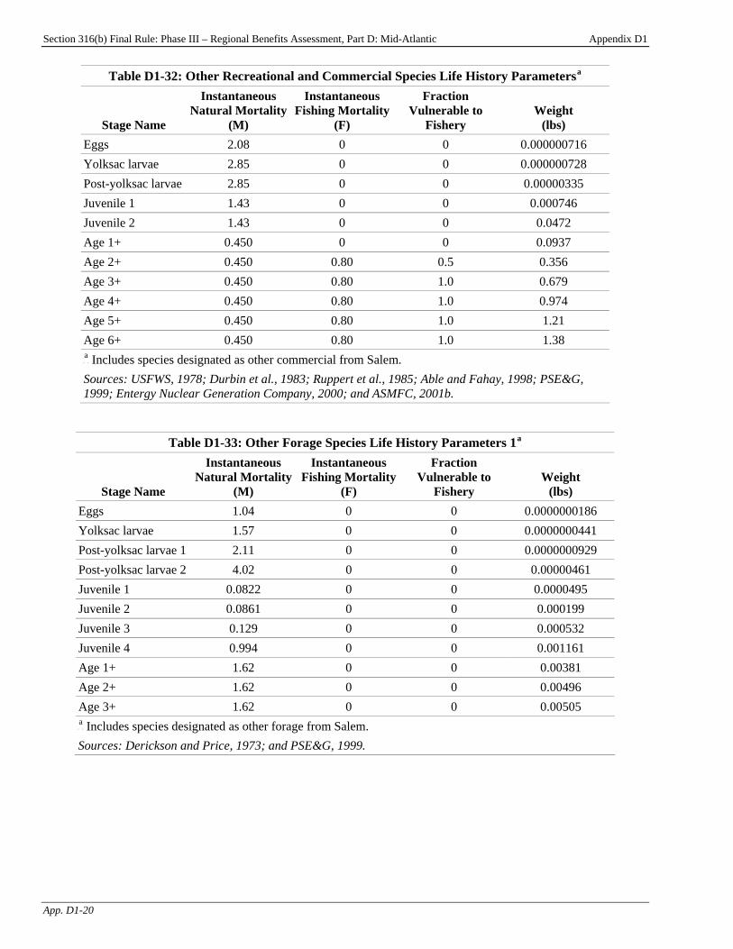
Section 316(b) Final Rule: Phase III – Regional Benefits Assessment, Part D: Mid-Atlantic Appendix D1
App. D1-20
Table D1-32: Other Recreational and Commercial Species Life History ParametersP
aP
Stage Name
Instantaneous Natural Mortality
(M)
Instantaneous Fishing Mortality
(F)
Fraction Vulnerable to
Fishery Weight
(lbs) Eggs 2.08 0 0 0.000000716 Yolksac larvae 2.85 0 0 0.000000728 Post-yolksac larvae 2.85 0 0 0.00000335 Juvenile 1 1.43 0 0 0.000746 Juvenile 2 1.43 0 0 0.0472 Age 1+ 0.450 0 0 0.0937 Age 2+ 0.450 0.80 0.5 0.356 Age 3+ 0.450 0.80 1.0 0.679 Age 4+ 0.450 0.80 1.0 0.974 Age 5+ 0.450 0.80 1.0 1.21 Age 6+ 0.450 0.80 1.0 1.38 P
aP Includes species designated as other commercial from Salem.
Sources: USFWS, 1978; Durbin et al., 1983; Ruppert et al., 1985; Able and Fahay, 1998; PSE&G, 1999; Entergy Nuclear Generation Company, 2000; and ASMFC, 2001b.
Table D1-33: Other Forage Species Life History Parameters 1P
aP
Stage Name
Instantaneous Natural Mortality
(M)
Instantaneous Fishing Mortality
(F)
Fraction Vulnerable to
Fishery Weight
(lbs) Eggs 1.04 0 0 0.0000000186 Yolksac larvae 1.57 0 0 0.0000000441 Post-yolksac larvae 1 2.11 0 0 0.0000000929 Post-yolksac larvae 2 4.02 0 0 0.00000461 Juvenile 1 0.0822 0 0 0.0000495 Juvenile 2 0.0861 0 0 0.000199 Juvenile 3 0.129 0 0 0.000532 Juvenile 4 0.994 0 0 0.001161 Age 1+ 1.62 0 0 0.00381 Age 2+ 1.62 0 0 0.00496 Age 3+ 1.62 0 0 0.00505 P
aP Includes species designated as other forage from Salem.
Sources: Derickson and Price, 1973; and PSE&G, 1999.
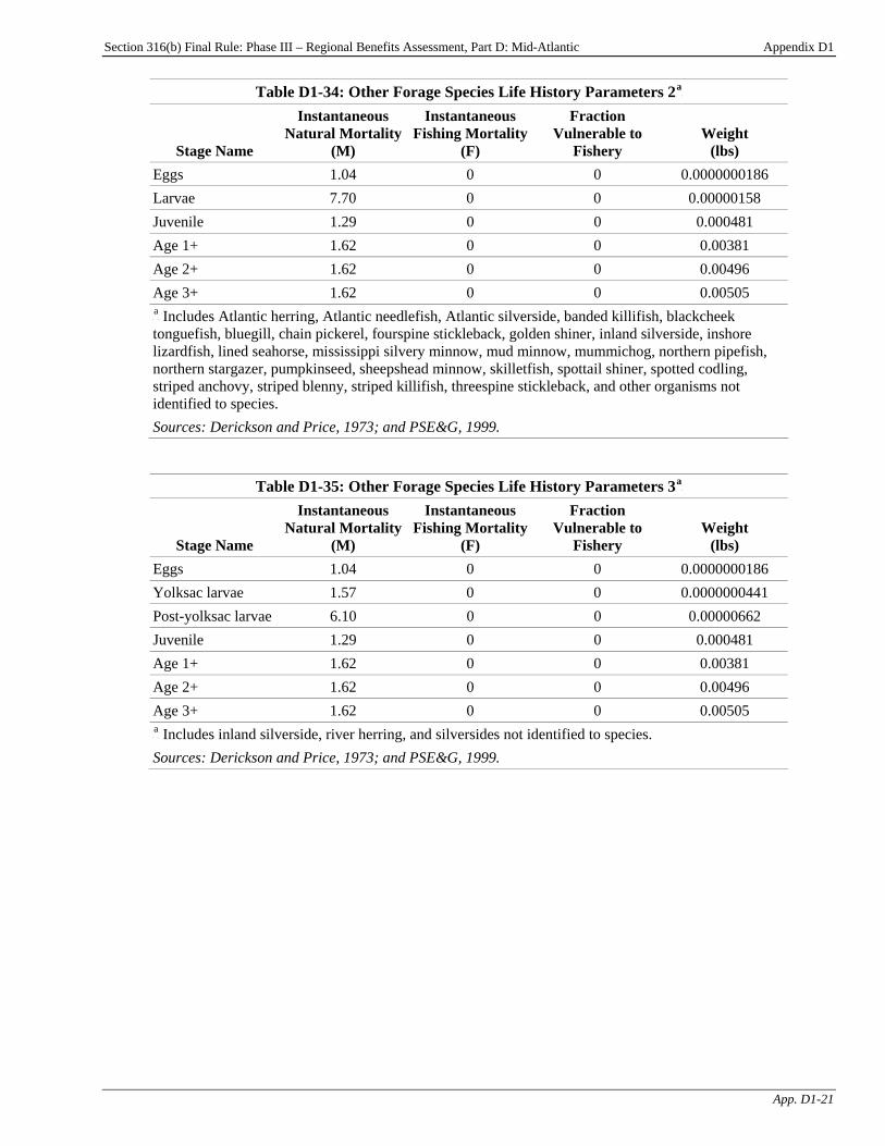
Section 316(b) Final Rule: Phase III – Regional Benefits Assessment, Part D: Mid-Atlantic Appendix D1
App. D1-21
Table D1-34: Other Forage Species Life History Parameters 2P
aP
Stage Name
Instantaneous Natural Mortality
(M)
Instantaneous Fishing Mortality
(F)
Fraction Vulnerable to
Fishery Weight
(lbs) Eggs 1.04 0 0 0.0000000186 Larvae 7.70 0 0 0.00000158 Juvenile 1.29 0 0 0.000481 Age 1+ 1.62 0 0 0.00381 Age 2+ 1.62 0 0 0.00496 Age 3+ 1.62 0 0 0.00505 P
aP Includes Atlantic herring, Atlantic needlefish, Atlantic silverside, banded killifish, blackcheek
tonguefish, bluegill, chain pickerel, fourspine stickleback, golden shiner, inland silverside, inshore lizardfish, lined seahorse, mississippi silvery minnow, mud minnow, mummichog, northern pipefish, northern stargazer, pumpkinseed, sheepshead minnow, skilletfish, spottail shiner, spotted codling, striped anchovy, striped blenny, striped killifish, threespine stickleback, and other organisms not identified to species. Sources: Derickson and Price, 1973; and PSE&G, 1999.
Table D1-35: Other Forage Species Life History Parameters 3P
aP
Stage Name
Instantaneous Natural Mortality
(M)
Instantaneous Fishing Mortality
(F)
Fraction Vulnerable to
Fishery Weight
(lbs) Eggs 1.04 0 0 0.0000000186 Yolksac larvae 1.57 0 0 0.0000000441 Post-yolksac larvae 6.10 0 0 0.00000662 Juvenile 1.29 0 0 0.000481 Age 1+ 1.62 0 0 0.00381 Age 2+ 1.62 0 0 0.00496 Age 3+ 1.62 0 0 0.00505 P
aP Includes inland silverside, river herring, and silversides not identified to species.
Sources: Derickson and Price, 1973; and PSE&G, 1999.
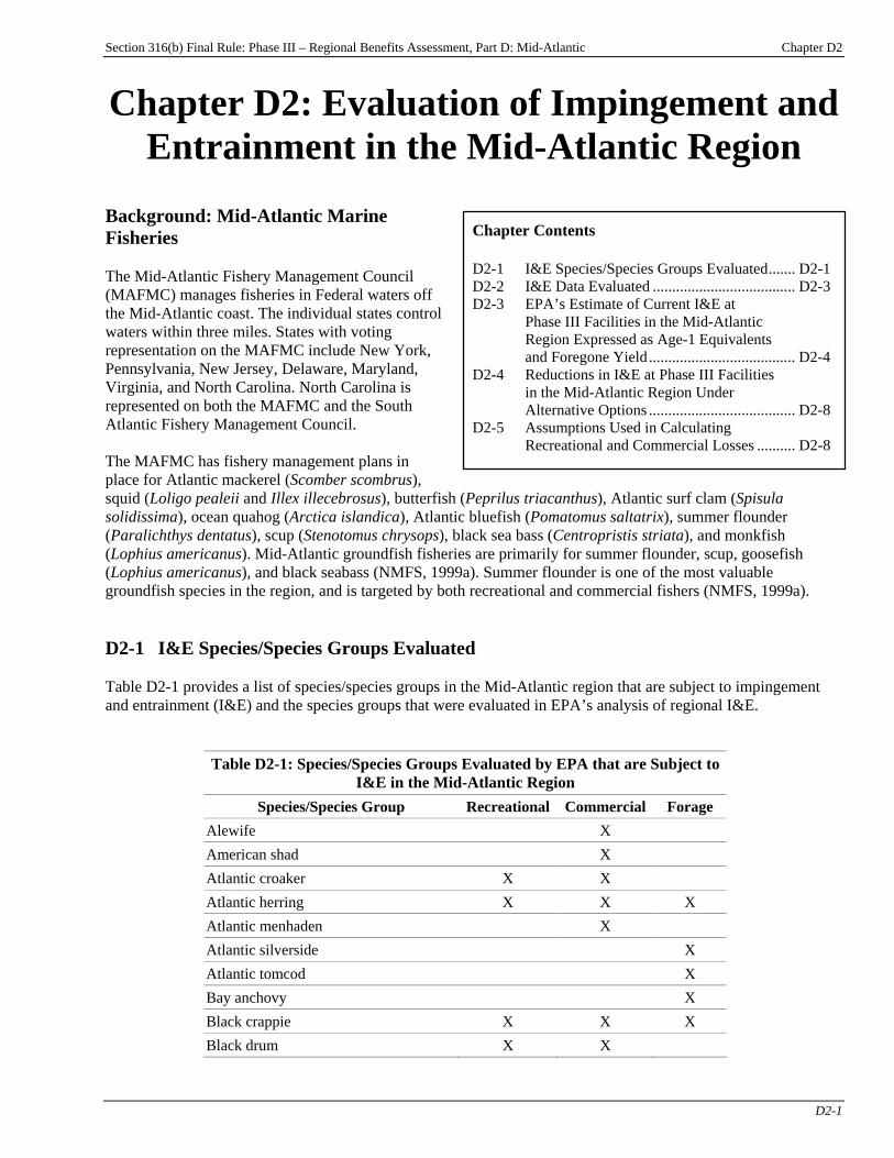
Section 316(b) Final Rule: Phase III – Regional Benefits Assessment, Part D: Mid-Atlantic Chapter D2
D2-1
Chapter D2: Evaluation of Impingement and Entrainment in the Mid-Atlantic Region
Background: Mid-Atlantic Marine Fisheries The Mid-Atlantic Fishery Management Council (MAFMC) manages fisheries in Federal waters off the Mid-Atlantic coast. The individual states control waters within three miles. States with voting representation on the MAFMC include New York, Pennsylvania, New Jersey, Delaware, Maryland, Virginia, and North Carolina. North Carolina is represented on both the MAFMC and the South Atlantic Fishery Management Council. The MAFMC has fishery management plans in place for Atlantic mackerel (Scomber scombrus), squid (Loligo pealeii and Illex illecebrosus), butterfish (Peprilus triacanthus), Atlantic surf clam (Spisula solidissima), ocean quahog (Arctica islandica), Atlantic bluefish (Pomatomus saltatrix), summer flounder (Paralichthys dentatus), scup (Stenotomus chrysops), black sea bass (Centropristis striata), and monkfish (Lophius americanus). Mid-Atlantic groundfish fisheries are primarily for summer flounder, scup, goosefish (Lophius americanus), and black seabass (NMFS, 1999a). Summer flounder is one of the most valuable groundfish species in the region, and is targeted by both recreational and commercial fishers (NMFS, 1999a). D2-1 I&E Species/Species Groups Evaluated Table D2-1 provides a list of species/species groups in the Mid-Atlantic region that are subject to impingement and entrainment (I&E) and the species groups that were evaluated in EPA’s analysis of regional I&E.
Table D2-1: Species/Species Groups Evaluated by EPA that are Subject to I&E in the Mid-Atlantic Region
Species/Species Group Recreational Commercial Forage Alewife X American shad X Atlantic croaker X X Atlantic herring X X X Atlantic menhaden X Atlantic silverside X Atlantic tomcod X Bay anchovy X Black crappie X X X Black drum X X
Chapter Contents D2-1 I&E Species/Species Groups Evaluated....... D2-1 D2-2 I&E Data Evaluated ..................................... D2-3 D2-3 EPA’s Estimate of Current I&E at Phase III Facilities in the Mid-Atlantic Region Expressed as Age-1 Equivalents and Foregone Yield...................................... D2-4 D2-4 Reductions in I&E at Phase III Facilities in the Mid-Atlantic Region Under Alternative Options ...................................... D2-8 D2-5 Assumptions Used in Calculating Recreational and Commercial Losses .......... D2-8
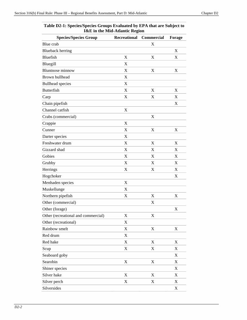
Section 316(b) Final Rule: Phase III – Regional Benefits Assessment, Part D: Mid-Atlantic Chapter D2
D2-2
Table D2-1: Species/Species Groups Evaluated by EPA that are Subject to I&E in the Mid-Atlantic Region
Species/Species Group Recreational Commercial Forage Blue crab X Blueback herring X Bluefish X X X Bluegill X Bluntnose minnow X X X Brown bullhead X Bullhead species X Butterfish X X X Carp X X X Chain pipefish X Channel catfish X Crabs (commercial) X Crappie X Cunner X X X Darter species X Freshwater drum X X X Gizzard shad X X X Gobies X X X Grubby X X X Herrings X X X Hogchoker X Menhaden species X Muskellunge X Northern pipefish X X X Other (commercial) X Other (forage) X Other (recreational and commercial) X X Other (recreational) X Rainbow smelt X X X Red drum X Red hake X X X Scup X X X Seaboard goby X Searobin X X X Shiner species X Silver hake X X X Silver perch X X X Silversides X
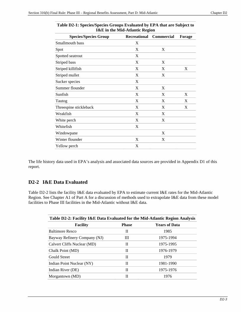
Section 316(b) Final Rule: Phase III – Regional Benefits Assessment, Part D: Mid-Atlantic Chapter D2
D2-3
Table D2-1: Species/Species Groups Evaluated by EPA that are Subject to I&E in the Mid-Atlantic Region
Species/Species Group Recreational Commercial Forage Smallmouth bass X Spot X X Spotted seatrout X Striped bass X X Striped killifish X X X Striped mullet X X Sucker species X Summer flounder X X Sunfish X X X Tautog X X X Threespine stickleback X X X Weakfish X X White perch X X Whitefish X Windowpane X Winter flounder X X Yellow perch X
The life history data used in EPA’s analysis and associated data sources are provided in Appendix D1 of this report. D2-2 I&E Data Evaluated Table D2-2 lists the facility I&E data evaluated by EPA to estimate current I&E rates for the Mid-Atlantic Region. See Chapter A1 of Part A for a discussion of methods used to extrapolate I&E data from these model facilities to Phase III facilities in the Mid-Atlantic without I&E data.
Table D2-2: Facility I&E Data Evaluated for the Mid-Atlantic Region AnalysisFacility Phase Years of Data
Baltimore Resco II 1985 Bayway Refinery Company (NJ) III 1975-1994 Calvert Cliffs Nuclear (MD) II 1975-1995 Chalk Point (MD) II 1976-1979 Gould Street II 1979 Indian Point Nuclear (NY) II 1981-1990 Indian River (DE) II 1975-1976 Morgantown (MD) II 1976
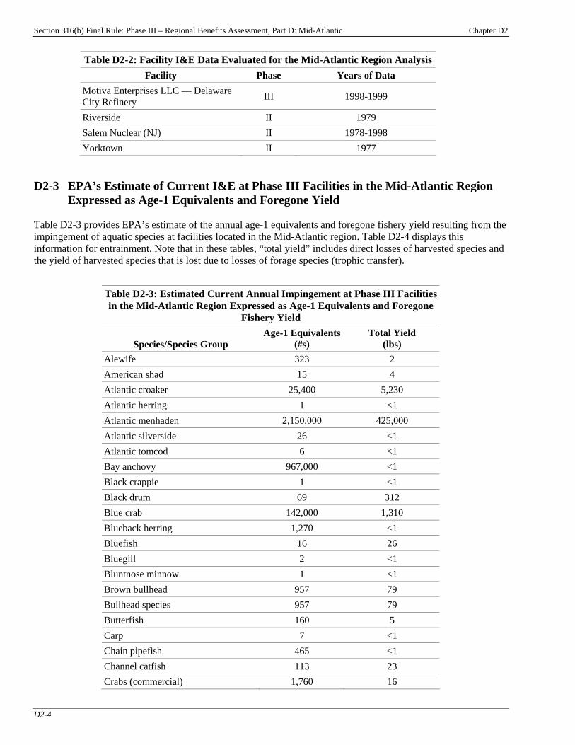
Section 316(b) Final Rule: Phase III – Regional Benefits Assessment, Part D: Mid-Atlantic Chapter D2
D2-4
Table D2-2: Facility I&E Data Evaluated for the Mid-Atlantic Region Analysis Facility Phase Years of Data
Motiva Enterprises LLC — Delaware City Refinery III 1998-1999
Riverside II 1979 Salem Nuclear (NJ) II 1978-1998 Yorktown II 1977
D2-3 EPA’s Estimate of Current I&E at Phase III Facilities in the Mid-Atlantic Region
Expressed as Age-1 Equivalents and Foregone Yield Table D2-3 provides EPA’s estimate of the annual age-1 equivalents and foregone fishery yield resulting from the impingement of aquatic species at facilities located in the Mid-Atlantic region. Table D2-4 displays this information for entrainment. Note that in these tables, “total yield” includes direct losses of harvested species and the yield of harvested species that is lost due to losses of forage species (trophic transfer).
Table D2-3: Estimated Current Annual Impingement at Phase III Facilities in the Mid-Atlantic Region Expressed as Age-1 Equivalents and Foregone
Fishery Yield
Species/Species Group Age-1 Equivalents
(#s) Total Yield
(lbs) Alewife 323 2 American shad 15 4 Atlantic croaker 25,400 5,230 Atlantic herring 1 <1 Atlantic menhaden 2,150,000 425,000 Atlantic silverside 26 <1 Atlantic tomcod 6 <1 Bay anchovy 967,000 <1 Black crappie 1 <1 Black drum 69 312 Blue crab 142,000 1,310 Blueback herring 1,270 <1 Bluefish 16 26 Bluegill 2 <1 Bluntnose minnow 1 <1 Brown bullhead 957 79 Bullhead species 957 79 Butterfish 160 5 Carp 7 <1 Chain pipefish 465 <1 Channel catfish 113 23 Crabs (commercial) 1,760 16
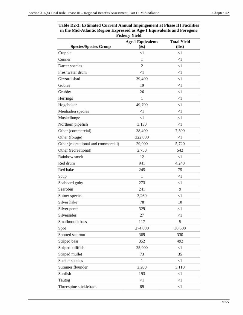
Section 316(b) Final Rule: Phase III – Regional Benefits Assessment, Part D: Mid-Atlantic Chapter D2
D2-5
Table D2-3: Estimated Current Annual Impingement at Phase III Facilities in the Mid-Atlantic Region Expressed as Age-1 Equivalents and Foregone
Fishery Yield
Species/Species Group Age-1 Equivalents
(#s) Total Yield
(lbs) Crappie <1 <1 Cunner 1 <1 Darter species 2 <1 Freshwater drum <1 <1 Gizzard shad 39,400 <1 Gobies 19 <1 Grubby 26 <1 Herrings 1 <1 Hogchoker 49,700 <1 Menhaden species <1 <1 Muskellunge <1 <1 Northern pipefish 3,130 <1 Other (commercial) 38,400 7,590 Other (forage) 322,000 <1 Other (recreational and commercial) 29,000 5,720 Other (recreational) 2,750 542 Rainbow smelt 12 <1 Red drum 941 4,240 Red hake 245 75 Scup 1 <1 Seaboard goby 273 <1 Searobin 241 9 Shiner species 3,260 <1 Silver hake 78 10 Silver perch 329 <1 Silversides 27 <1 Smallmouth bass 117 5 Spot 274,000 30,600 Spotted seatrout 369 330 Striped bass 352 492 Striped killifish 25,900 <1 Striped mullet 73 35 Sucker species 1 <1 Summer flounder 2,200 3,110 Sunfish 193 <1 Tautog <1 <1 Threespine stickleback 89 <1
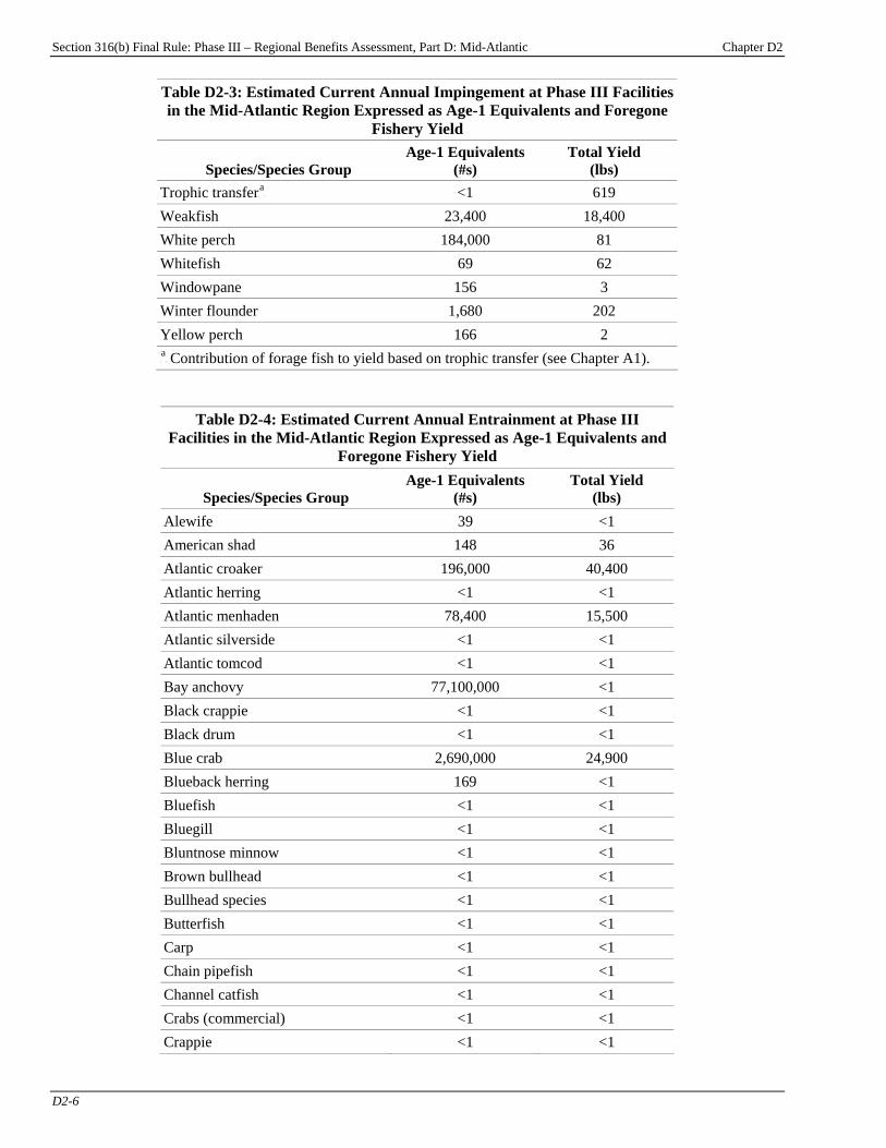
Section 316(b) Final Rule: Phase III – Regional Benefits Assessment, Part D: Mid-Atlantic Chapter D2
D2-6
Table D2-3: Estimated Current Annual Impingement at Phase III Facilities in the Mid-Atlantic Region Expressed as Age-1 Equivalents and Foregone
Fishery Yield
Species/Species Group Age-1 Equivalents
(#s) Total Yield
(lbs) Trophic transferP
aP <1 619
Weakfish 23,400 18,400 White perch 184,000 81 Whitefish 69 62 Windowpane 156 3 Winter flounder 1,680 202 Yellow perch 166 2 P
aP Contribution of forage fish to yield based on trophic transfer (see Chapter A1).
Table D2-4: Estimated Current Annual Entrainment at Phase III Facilities in the Mid-Atlantic Region Expressed as Age-1 Equivalents and
Foregone Fishery Yield
Species/Species Group Age-1 Equivalents
(#s) Total Yield
(lbs) Alewife 39 <1 American shad 148 36 Atlantic croaker 196,000 40,400 Atlantic herring <1 <1 Atlantic menhaden 78,400 15,500 Atlantic silverside <1 <1 Atlantic tomcod <1 <1 Bay anchovy 77,100,000 <1 Black crappie <1 <1 Black drum <1 <1 Blue crab 2,690,000 24,900 Blueback herring 169 <1 Bluefish <1 <1 Bluegill <1 <1 Bluntnose minnow <1 <1 Brown bullhead <1 <1 Bullhead species <1 <1 Butterfish <1 <1 Carp <1 <1 Chain pipefish <1 <1 Channel catfish <1 <1 Crabs (commercial) <1 <1 Crappie <1 <1
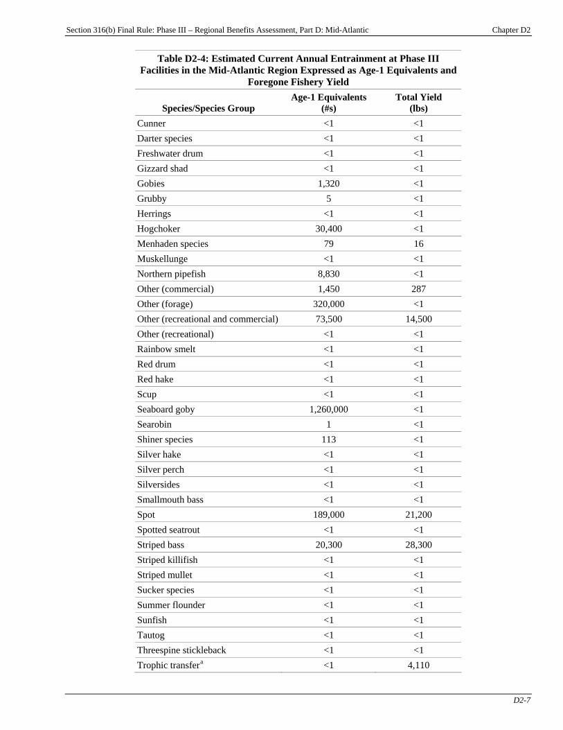
Section 316(b) Final Rule: Phase III – Regional Benefits Assessment, Part D: Mid-Atlantic Chapter D2
D2-7
Table D2-4: Estimated Current Annual Entrainment at Phase III Facilities in the Mid-Atlantic Region Expressed as Age-1 Equivalents and
Foregone Fishery Yield
Species/Species Group Age-1 Equivalents
(#s) Total Yield
(lbs) Cunner <1 <1 Darter species <1 <1 Freshwater drum <1 <1 Gizzard shad <1 <1 Gobies 1,320 <1 Grubby 5 <1 Herrings <1 <1 Hogchoker 30,400 <1 Menhaden species 79 16 Muskellunge <1 <1 Northern pipefish 8,830 <1 Other (commercial) 1,450 287 Other (forage) 320,000 <1 Other (recreational and commercial) 73,500 14,500 Other (recreational) <1 <1 Rainbow smelt <1 <1 Red drum <1 <1 Red hake <1 <1 Scup <1 <1 Seaboard goby 1,260,000 <1 Searobin 1 <1 Shiner species 113 <1 Silver hake <1 <1 Silver perch <1 <1 Silversides <1 <1 Smallmouth bass <1 <1 Spot 189,000 21,200 Spotted seatrout <1 <1 Striped bass 20,300 28,300 Striped killifish <1 <1 Striped mullet <1 <1 Sucker species <1 <1 Summer flounder <1 <1 Sunfish <1 <1 Tautog <1 <1 Threespine stickleback <1 <1 Trophic transferP
aP <1 4,110
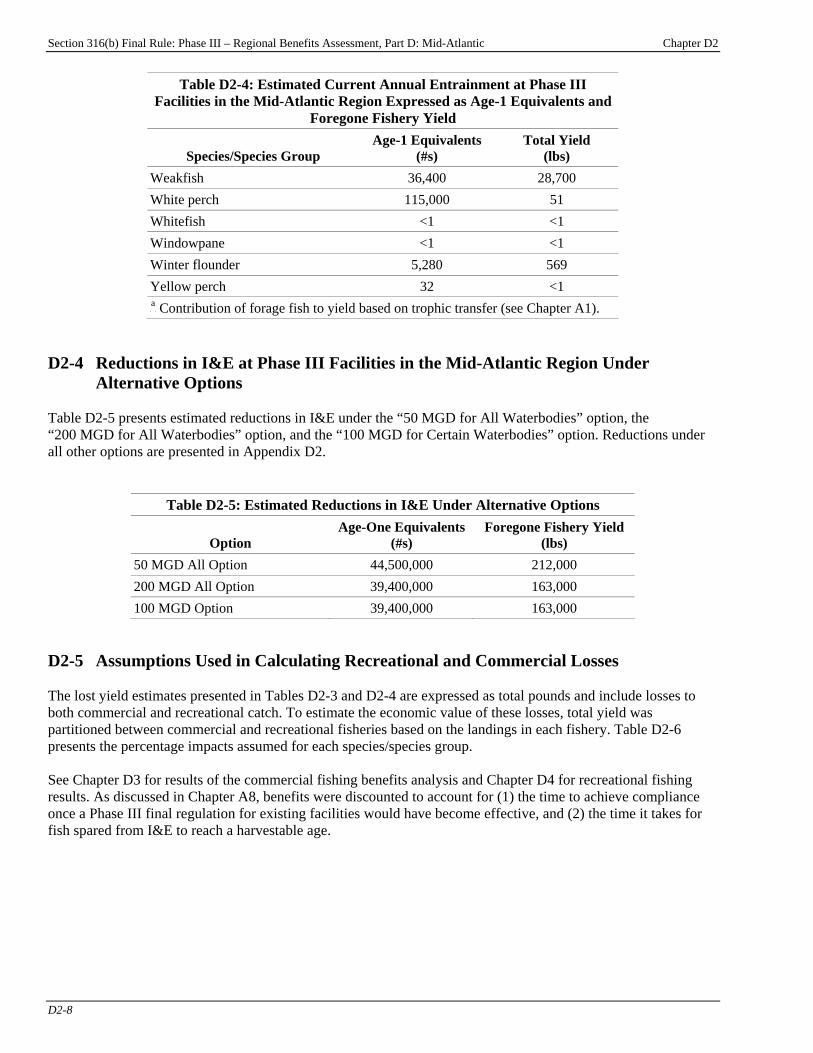
Section 316(b) Final Rule: Phase III – Regional Benefits Assessment, Part D: Mid-Atlantic Chapter D2
D2-8
Table D2-4: Estimated Current Annual Entrainment at Phase III Facilities in the Mid-Atlantic Region Expressed as Age-1 Equivalents and
Foregone Fishery Yield
Species/Species Group Age-1 Equivalents
(#s) Total Yield
(lbs) Weakfish 36,400 28,700 White perch 115,000 51 Whitefish <1 <1 Windowpane <1 <1 Winter flounder 5,280 569 Yellow perch 32 <1 P
aP Contribution of forage fish to yield based on trophic transfer (see Chapter A1).
D2-4 Reductions in I&E at Phase III Facilities in the Mid-Atlantic Region Under
Alternative Options Table D2-5 presents estimated reductions in I&E under the “50 MGD for All Waterbodies” option, the “200 MGD for All Waterbodies” option, and the “100 MGD for Certain Waterbodies” option. Reductions under all other options are presented in Appendix D2.
Table D2-5: Estimated Reductions in I&E Under Alternative Options
Option Age-One Equivalents
(#s) Foregone Fishery Yield
(lbs) 50 MGD All Option 44,500,000 212,000 200 MGD All Option 39,400,000 163,000 100 MGD Option 39,400,000 163,000
D2-5 Assumptions Used in Calculating Recreational and Commercial Losses The lost yield estimates presented in Tables D2-3 and D2-4 are expressed as total pounds and include losses to both commercial and recreational catch. To estimate the economic value of these losses, total yield was partitioned between commercial and recreational fisheries based on the landings in each fishery. Table D2-6 presents the percentage impacts assumed for each species/species group. See Chapter D3 for results of the commercial fishing benefits analysis and Chapter D4 for recreational fishing results. As discussed in Chapter A8, benefits were discounted to account for (1) the time to achieve compliance once a Phase III final regulation for existing facilities would have become effective, and (2) the time it takes for fish spared from I&E to reach a harvestable age.

Section 316(b) Final Rule: Phase III – Regional Benefits Assessment, Part D: Mid-Atlantic Chapter D2
D2-9
Table D2-6: Percentage of Total Impacts Occurring to the Commercial and Recreational Fisheries and Commercial Value per Pound for Species Impinged and Entrained at
Mid-Atlantic Facilities
Species/Species Group Percent Impact to
Recreational FisheryP
a,bP
Percent Impact to Commercial FisheryP
a,bP
Alewife 0.0% 100.0% American plaice 0.0% 100.0% American shad 0.0% 100.0% Atlantic cod 50.0% 50.0% Atlantic croaker 66.4% 33.6% Atlantic herring 19.0% 81.0% Atlantic mackerel 22.2% 77.8% Atlantic menhaden 0.0% 100.0% Bigmouth buffalo 100.0% 0.0% Black bullhead 100.0% 0.0% Black crappie 100.0% 0.0% Black drum 93.0% 7.0% Blue crab 0.0% 100.0% Bluefish 89.1% 10.9% Bluegill 100.0% 0.0% Brown bullhead 100.0% 0.0% Bullhead species 100.0% 0.0% Butterfish 0.0% 100.0% Channel catfish 100.0% 0.0% Crabs (commercial) 0.0% 100.0% Crappie 100.0% 0.0% Cunner 100.0% 0.0% Darter species 100.0% 0.0% Drums and croakers 69.1% 30.9% Flounders 100.0% 0.0% Freshwater drum 100.0% 0.0% Golden redhorse 100.0% 0.0% Leatherjacket 0.0% 100.0% Logperch 100.0% 0.0% Mackerels 73.5% 26.5% Menhaden species 100.0% 0.0% Muskellunge 100.0% 0.0% Other (commercial) 0.0% 100.0% Other (recreational and commercial)P
cP 50.0% 50.0%
Other (recreational) 100.0% 0.0% Paddlefish 100.0% 0.0% Pinfish 100.0% 0.0% Pink shrimp 100.0% 0.0% Pollock 50.0% 50.0%
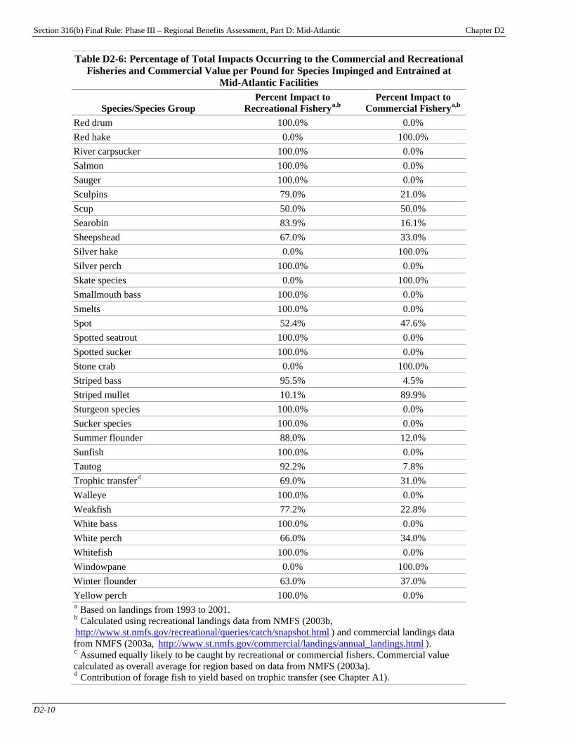
Section 316(b) Final Rule: Phase III – Regional Benefits Assessment, Part D: Mid-Atlantic Chapter D2
D2-10
Table D2-6: Percentage of Total Impacts Occurring to the Commercial and Recreational Fisheries and Commercial Value per Pound for Species Impinged and Entrained at
Mid-Atlantic Facilities
Species/Species Group Percent Impact to
Recreational FisheryP
a,bP
Percent Impact to Commercial FisheryP
a,bP
Red drum 100.0% 0.0% Red hake 0.0% 100.0% River carpsucker 100.0% 0.0% Salmon 100.0% 0.0% Sauger 100.0% 0.0% Sculpins 79.0% 21.0% Scup 50.0% 50.0% Searobin 83.9% 16.1% Sheepshead 67.0% 33.0% Silver hake 0.0% 100.0% Silver perch 100.0% 0.0% Skate species 0.0% 100.0% Smallmouth bass 100.0% 0.0% Smelts 100.0% 0.0% Spot 52.4% 47.6% Spotted seatrout 100.0% 0.0% Spotted sucker 100.0% 0.0% Stone crab 0.0% 100.0% Striped bass 95.5% 4.5% Striped mullet 10.1% 89.9% Sturgeon species 100.0% 0.0% Sucker species 100.0% 0.0% Summer flounder 88.0% 12.0% Sunfish 100.0% 0.0% Tautog 92.2% 7.8% Trophic transferP
dP 69.0% 31.0%
Walleye 100.0% 0.0% Weakfish 77.2% 22.8% White bass 100.0% 0.0% White perch 66.0% 34.0% Whitefish 100.0% 0.0% Windowpane 0.0% 100.0% Winter flounder 63.0% 37.0% Yellow perch 100.0% 0.0% P
aP Based on landings from 1993 to 2001.
P
bP Calculated using recreational landings data from NMFS (2003b,
HTUhttp://www.st.nmfs.gov/recreational/queries/catch/snapshot.htmlUTH) and commercial landings data from NMFS (2003a, HTUhttp://www.st.nmfs.gov/commercial/landings/annual_landings.htmlUTH). P
cP Assumed equally likely to be caught by recreational or commercial fishers. Commercial value
calculated as overall average for region based on data from NMFS (2003a). P
dP Contribution of forage fish to yield based on trophic transfer (see Chapter A1).
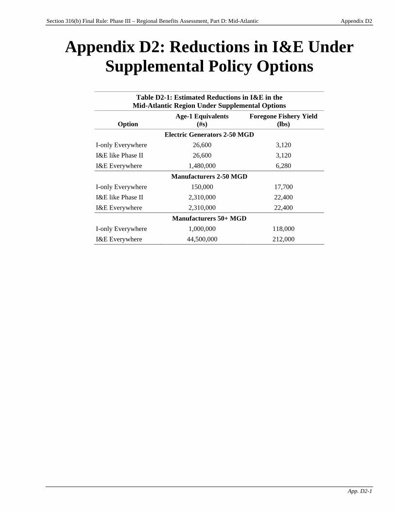
Section 316(b) Final Rule: Phase III – Regional Benefits Assessment, Part D: Mid-Atlantic Appendix D2
App. D2-1
Appendix D2: Reductions in I&E Under Supplemental Policy Options
Table D2-1: Estimated Reductions in I&E in the Mid-Atlantic Region Under Supplemental Options
Option Age-1 Equivalents
(#s) Foregone Fishery Yield
(lbs) Electric Generators 2-50 MGD
I-only Everywhere 26,600 3,120 I&E like Phase II 26,600 3,120 I&E Everywhere 1,480,000 6,280
Manufacturers 2-50 MGD I-only Everywhere 150,000 17,700 I&E like Phase II 2,310,000 22,400 I&E Everywhere 2,310,000 22,400
Manufacturers 50+ MGD I-only Everywhere 1,000,000 118,000 I&E Everywhere 44,500,000 212,000
Section 316(b) Final Rule: Phase III – Regional Benefits Assessment, Part D: Mid-Atlantic Chapter D3
D3-1
Chapter D3: Commercial Fishing Benefits Introduction
Chapter Contents D3-1 Baseline Commercial Losses ....................... D3-1 D3-2 Expected Benefits Under Regulatory Analysis Options .......................................... D3-3
D3-2.1 Commercial Fishing Benefits of the “50 MGD for All Waterbodies” Option............................................. D3-4 D3-2.2 Commercial Fishing Benefits of the “200 MGD for All Waterbodies” Option............................................. D3-4
D3-2.3 Commercial Fishing Benefits of the “100 MGD for Certain Waterbodies” Option ...................... D3-5
This chapter presents the results of the commercial fishing benefits analysis for the Mid-Atlantic region. The chapter presents EPA’s estimates of baseline (i.e., current) annual commercial fishery losses from impingement and entrainment (I&E) at potentially regulated facilities in the Mid-Atlantic region and annual reductions in these losses under the regulatory options for Phase III existing facilitiesPF
1FP:
< the “50 MGD for All Waterbodies” option, < the “200 MGD for All Waterbodies” option,
and < the “100 MGD for Certain Waterbodies”
option. The chapter then presents the estimated benefits to commercial fisheries from eliminating baseline losses from I&E, and the expected benefits under the regulatory options. Chapter A4, “Methods for Estimating Commercial Fishing Benefits,” details the methods used by EPA to estimate the commercial fishing benefits of reducing and eliminating I&E losses. EPA considered a wide range of policy options in developing this regulation. In addition to the regulatory options, EPA evaluated several supplemental options. Appendix D3 presents results of the commercial fishing benefits analysis for the supplemental options. For more information on the options, please see the TDD. D3-1 Baseline Commercial Losses Table D3-1 provides EPA’s estimate of the value of gross revenues lost in commercial fisheries resulting from the impingement of aquatic species at facilities in the Mid-Atlantic region. Table D3-2 displays this information for entrainment. Total annualized revenue losses are approximately $89,236 (undiscounted).
P
1P See the Introduction to this report for a description of the primary analysis options.
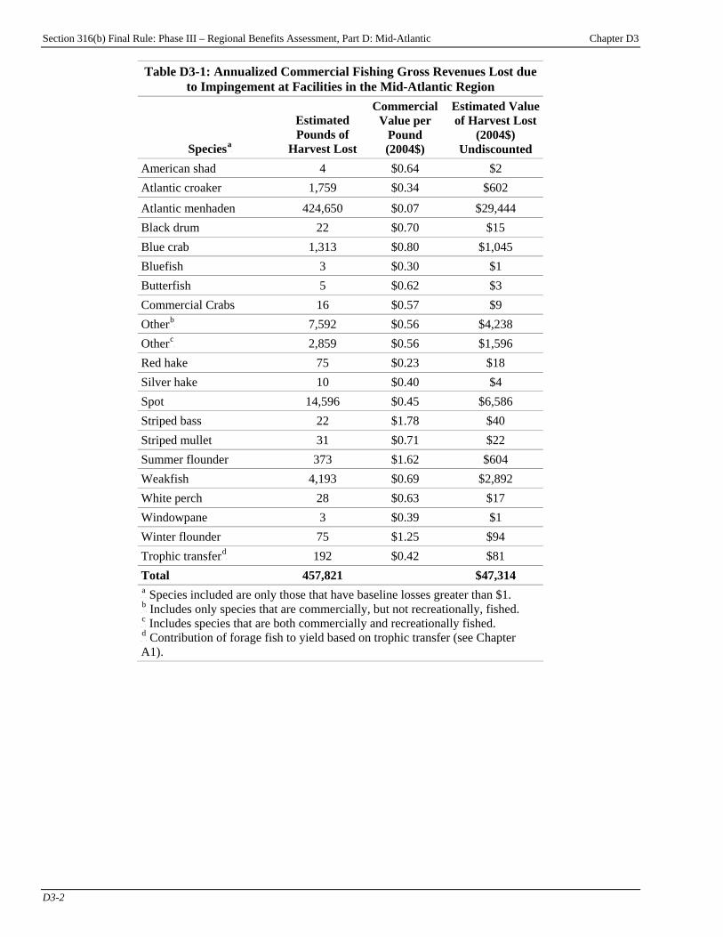
Section 316(b) Final Rule: Phase III – Regional Benefits Assessment, Part D: Mid-Atlantic Chapter D3
D3-2
Table D3-1: Annualized Commercial Fishing Gross Revenues Lost due to Impingement at Facilities in the Mid-Atlantic Region
SpeciesP
aP
Estimated Pounds of
Harvest Lost
Commercial Value per
Pound (2004$)
Estimated Value of Harvest Lost
(2004$) Undiscounted
American shad 4 $0.64 $2 Atlantic croaker 1,759 $0.34 $602
Atlantic menhaden 424,650 $0.07 $29,444 Black drum 22 $0.70 $15 Blue crab 1,313 $0.80 $1,045 Bluefish 3 $0.30 $1 Butterfish 5 $0.62 $3 Commercial Crabs 16 $0.57 $9 OtherP
bP 7,592 $0.56 $4,238
OtherP
cP 2,859 $0.56 $1,596
Red hake 75 $0.23 $18 Silver hake 10 $0.40 $4 Spot 14,596 $0.45 $6,586 Striped bass 22 $1.78 $40 Striped mullet 31 $0.71 $22 Summer flounder 373 $1.62 $604 Weakfish 4,193 $0.69 $2,892 White perch 28 $0.63 $17 Windowpane 3 $0.39 $1 Winter flounder 75 $1.25 $94 Trophic transferP
dP 192 $0.42 $81
Total 457,821 $47,314 P
aP Species included are only those that have baseline losses greater than $1.
P
bP Includes only species that are commercially, but not recreationally, fished.
P
cP Includes species that are both commercially and recreationally fished.
P
dP Contribution of forage fish to yield based on trophic transfer (see Chapter
A1).

Section 316(b) Final Rule: Phase III – Regional Benefits Assessment, Part D: Mid-Atlantic Chapter D3
D3-3
Table D3-2: Annualized Commercial Fishing Gross Revenues Lost due to Entrainment at Facilities in the Mid-Atlantic Region
SpeciesP
aP
Estimated Pounds of
Harvest Lost
Commercial Value per
Pound (2004$)
Estimated Value of Harvest Lost
(2004$) Undiscounted
American shad 36 $0.64 $23 Atlantic croaker 13,599 $0.34 $4,655
Atlantic menhaden 15,491 $0.07 $1,074 Blue crab 24,865 $0.80 $19,796 OtherP
bP 287 $0.56 $160
OtherP
cP 7,262 $0.56 $4,054
Spot 10,108 $0.45 $4,561 Striped bass 1,283 $1.78 $2,281 Weakfish 6,523 $0.69 $4,499 White perch 17 $0.63 $11 Winter flounder 211 $1.25 $264 Trophic transferP
dP 1,274 $0.42 $539
Total 80,956 $41,917 P
aP Species included are only those that have baseline losses greater than $1.
P
bP Includes only species that are commercially, but not recreationally, fished.
P
cP Include species that are both commercially and recreationally fished.
P
dP Contribution of forage fish to yield based on trophic transfer (see Chapter
A1). D3-2 Expected Benefits Under Regulatory Analysis Options As described in Chapter A4, EPA estimates for Mid-Atlantic that, depending on species, 0 to 84% of the gross revenue losses represent surplus losses to producers, assuming no change in prices or fishing costs. Earlier EPA analysis assumed a rate of 40%. The 0% estimate, of course, results in loss estimates of $0. The expected reductions in I&E attributable to changes at facilities required by the “50 MGD for All Waterbodies” option (50 MGD All option) are 23.4% for impingement and 52.9% for entrainment; the expected reductions for the “200 MGD for All Waterbodies” option (200 MGD All option) are 15.6% for impingement and 47.1% for entrainment; and the expected reductions for the “100 MGD for Certain Waterbodies” option (100 MGD CWB option) are 15.6% for impingement 47.1% for entrainment. Total annualized benefits are estimated by applying these estimated reductions to the annual baseline producer surplus loss. As presented in Tables D3-3, D3-4, and D3-5, this results in total annualized benefits of up to approximately $18,387 for the 50 MGD All option, $14,848 for the 200 MGD All option, and $14,848 for the 100 MGD CWB option, assuming a 3% discount rate and a species-specific net benefits ratio.TPF
2FPT
TP
2PT The net benefits ratio is the fractional share of gross revenue associated with net benefits, by gear and vessel type.
See Chapter A4, section A4-10, for a description of the species-specific net benefits ratios and how they are calculated.
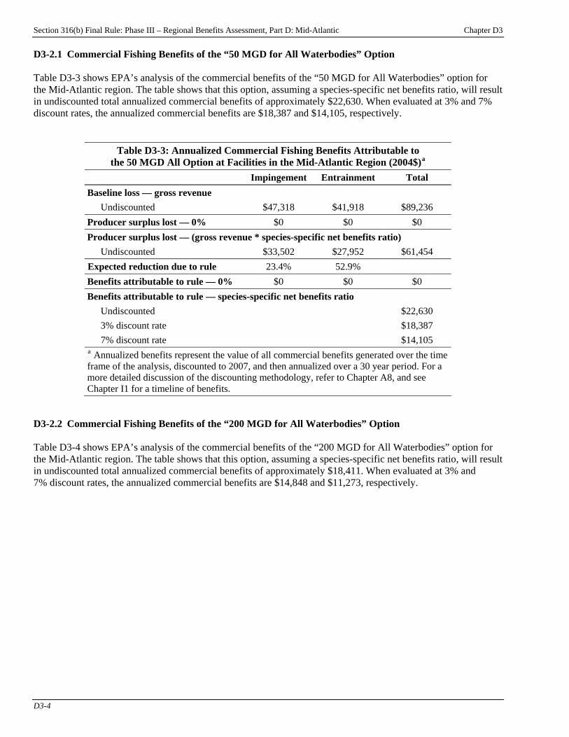
Section 316(b) Final Rule: Phase III – Regional Benefits Assessment, Part D: Mid-Atlantic Chapter D3
D3-4
D3-2.1 Commercial Fishing Benefits of the “50 MGD for All Waterbodies” Option Table D3-3 shows EPA’s analysis of the commercial benefits of the “50 MGD for All Waterbodies” option for the Mid-Atlantic region. The table shows that this option, assuming a species-specific net benefits ratio, will result in undiscounted total annualized commercial benefits of approximately $22,630. When evaluated at 3% and 7% discount rates, the annualized commercial benefits are $18,387 and $14,105, respectively.
Table D3-3: Annualized Commercial Fishing Benefits Attributable to the 50 MGD All Option at Facilities in the Mid-Atlantic Region (2004$)P
aP
Impingement Entrainment Total Baseline loss — gross revenue
Undiscounted $47,318 $41,918 $89,236 Producer surplus lost — 0% $0 $0 $0 Producer surplus lost — (gross revenue * species-specific net benefits ratio)
Undiscounted $33,502 $27,952 $61,454 Expected reduction due to rule 23.4% 52.9% Benefits attributable to rule — 0% $0 $0 $0 Benefits attributable to rule — species-specific net benefits ratio
Undiscounted $22,630 3% discount rate $18,387 7% discount rate $14,105
P
aP Annualized benefits represent the value of all commercial benefits generated over the time
frame of the analysis, discounted to 2007, and then annualized over a 30 year period. For a more detailed discussion of the discounting methodology, refer to Chapter A8, and see Chapter I1 for a timeline of benefits.
D3-2.2 Commercial Fishing Benefits of the “200 MGD for All Waterbodies” Option Table D3-4 shows EPA’s analysis of the commercial benefits of the “200 MGD for All Waterbodies” option for the Mid-Atlantic region. The table shows that this option, assuming a species-specific net benefits ratio, will result in undiscounted total annualized commercial benefits of approximately $18,411. When evaluated at 3% and 7% discount rates, the annualized commercial benefits are $14,848 and $11,273, respectively.

Section 316(b) Final Rule: Phase III – Regional Benefits Assessment, Part D: Mid-Atlantic Chapter D3
D3-5
Table D3-4: Annualized Commercial Fishing Benefits Attributable to the 200 MGD All Option at Facilities in the Mid-Atlantic Region (2004$)P
aP
Impingement Entrainment Total Baseline loss — gross revenue
Undiscounted $47,318 $41,918 $89,236 Producer surplus lost — 0% $0 $0 $0 Producer surplus lost — (gross revenue * species-specific net benefits ratio)
Undiscounted $33,502 $27,952 $61,454 Expected reduction due to rule 15.6% 47.1% Benefits attributable to rule — 0% $0 $0 $0 Benefits attributable to rule — species-specific net benefits ratio
Undiscounted $18,411 3% discount rate $14,848 7% discount rate $11,273
P
aP Annualized benefits represent the value of all commercial benefits generated over the time
frame of the analysis, discounted to 2007, and then annualized over a 30 year period. For a more detailed discussion of the discounting methodology, refer to Chapter A8, and see Chapter I1 for a timeline of benefits.
D3-2.3 Commercial Fishing Benefits of the “100 MGD for Certain Waterbodies” Option Table D3-5 shows EPA’s analysis of the commercial benefits of the “100 MGD for Certain Waterbodies” option for the Mid-Atlantic region. The table shows that this option, assuming a species-specific net benefits ratio, will result in undiscounted total annualized commercial benefits of approximately $18,411. When evaluated at 3% and 7% discount rates, the annualized commercial benefits are $14,848 and $11,273, respectively.
Table D3-5: Annualized Commercial Fishing Benefits Attributable to the 100 MGD CWB Option at Facilities in the Mid-Atlantic Region (2004$)P
aP
Impingement Entrainment Total Baseline loss — gross revenue
Undiscounted $47,318 $41,918 $89,236 Producer surplus lost — 0% $0 $0 $0 Producer surplus lost — (gross revenue * species-specific net benefits ratio)
Undiscounted $33,502 $27,952 $61,454 Expected reduction due to rule 15.6% 47.1% Benefits attributable to rule — 0% $0 $0 $0 Benefits attributable to rule — species-specific net benefits ratio
Undiscounted $18,411 3% discount rate $14,848 7% discount rate $11,273
P
aP Annualized benefits represent the value of all commercial benefits generated over the time
frame of the analysis, discounted to 2007, and then annualized over a 30 year period. For a more detailed discussion of the discounting methodology, refer to Chapter A8, and see Chapter I1 for a timeline of benefits.

Section 316(b) Final Rule: Phase III – Regional Benefits Assessment, Part D: Mid-Atlantic Appendix D3
App. D3-1
Appendix D3: Commercial Fishing Benefits Under Supplemental Policy Options
Introduction Chapter D3 presents EPA’s estimates of the commercial benefits of the regulatory options for the section 316(b) rule for Phase III facilities in the Mid-Atlantic region. To facilitate comparisons among the options, this appendix presents estimates of the commercial fishing benefits of several supplemental options that EPA evaluated in preparation for this rule:
Appendix Contents D3-1 Commercial Fishing Benefits of the Supplemental Options ................................ D3-2
< “Electric Generators 2-50 MGD I-only Everywhere” option; < “Electric Generators 2-50 MGD I&E like Phase II” option; < “Electric Generators 2-50 MGD I&E Everywhere” option; < “Manufacturers 2-50 MGD I-only Everywhere” option; < “Manufacturers 2-50 MGD I&E like Phase II” option; < “Manufacturers 2-50 MGD I&E Everywhere” option; < “Manufacturers 50+ MGD I-only Everywhere” option; and < “Manufacturers 50+ MGD I&E Everywhere” option.
Commercial fishing benefits presented in this chapter were estimated using the benefit transfer approach discussed in Chapter D3 and in Chapter A4, “Methods for Estimating Commercial Fishing Benefits.”

Section 316(b) Final Rule: Phase III – Regional Benefits Assessment, Part D: Mid-Atlantic Appendix D3
App. D3-2
D3-1 Commercial Fishing Benefits of the Supplemental Options Tables D3-1 through D3-8 present EPA’s estimates of the annualized commercial benefits of the supplemental options in the Mid-Atlantic region. For more information on the options, please see the TDD.
Table D3-1: Annualized Commercial Fishing Benefits Attributable to the “Electric Generators 2-50 MGD I-only Everywhere” Option at Facilities in the
Mid-Atlantic Region (2004$)P
aP
Impingement Entrainment Total Baseline loss — gross revenue
Undiscounted $47,318 $41,918 $89,236 Producer surplus lost — 0% $0 $0 $0 Producer surplus lost — (gross revenue * species-specific net benefits ratio)
Undiscounted $33,502 $27,952 $61,454 Expected reduction due to rule 1% 0% Benefits attributable to rule — 0% $0 $0 $0 Benefits attributable to rule — species-specific net benefits ratio
Undiscounted $207 3% discount rate $159 7% discount rate $113
P
aP Annualized benefits represent the value of all commercial benefits generated over the time
frame of the analysis, discounted to 2007, and then annualized over a thirty year period. For a more detailed discussion of the discounting methodology, refer to Chapter A8, and see Chapter I1 for a timeline of benefits.
Table D3-2: Annualized Commercial Fishing Benefits Attributable to the “Electric Generators 2-50 MGD I&E like Phase II” Option at Facilities in the
Mid-Atlantic Region (2004$)P
aP
Impingement Entrainment Total Baseline loss — gross revenue
Undiscounted $47,318 $41,918 $89,236 Producer surplus lost — 0% $0 $0 $0 Producer surplus lost — (gross revenue * species-specific net benefits ratio)
Undiscounted $33,502 $27,952 $61,454 Expected reduction due to rule 1% 0% Benefits attributable to rule — 0% $0 $0 $0 Benefits attributable to rule — species-specific net benefits ratio
Undiscounted $207 3% discount rate $159 7% discount rate $113
P
aP Annualized benefits represent the value of all commercial benefits generated over the time
frame of the analysis, discounted to 2007, and then annualized over a thirty year period. For a more detailed discussion of the discounting methodology, refer to Chapter A8, and see Chapter I1 for a timeline of benefits.

Section 316(b) Final Rule: Phase III – Regional Benefits Assessment, Part D: Mid-Atlantic Appendix D3
App. D3-3
Table D3-3: Annualized Commercial Fishing Benefits Attributable to the “Electric Generators 2-50 MGD I&E Everywhere” Option at Facilities in the
Mid-Atlantic Region (2004$)P
aP
Impingement Entrainment Total Baseline loss — gross revenue
Undiscounted $47,318 $41,918 $89,236 Producer surplus lost — 0% $0 $0 $0 Producer surplus lost — (gross revenue * species-specific net benefits ratio)
Undiscounted $33,502 $27,952 $61,454 Expected reduction due to rule 1% 2% Benefits attributable to rule — 0% $0 $0 $0 Benefits attributable to rule — species-specific net benefits ratio
Undiscounted $701 3% discount rate $566 7% discount rate $432
P
aP Annualized benefits represent the value of all commercial benefits generated over the time
frame of the analysis, discounted to 2007, and then annualized over a thirty year period. For a more detailed discussion of the discounting methodology, refer to Chapter A8, and see Chapter I1 for a timeline of benefits.
Table D3-4: Annualized Commercial Fishing Benefits Attributable to the “Manufacturers 2-50 MGD I-only Everywhere” Option at Facilities in the
Mid-Atlantic Region (2004$)P
aP
Impingement Entrainment Total Baseline loss — gross revenue
Undiscounted $47,318 $41,918 $89,236 Producer surplus lost — 0% $0 $0 $0 Producer surplus lost — (gross revenue * species-specific net benefits ratio)
Undiscounted $33,502 $27,952 $61,454 Expected reduction due to rule 4% 0% Benefits attributable to rule — 0% $0 $0 $0 Benefits attributable to rule — species-specific net benefits ratio
Undiscounted $1,174 3% discount rate $982 7% discount rate $782
P
aP Annualized benefits represent the value of all commercial benefits generated over the time
frame of the analysis, discounted to 2007, and then annualized over a thirty year period. For a more detailed discussion of the discounting methodology, refer to Chapter A8, and see Chapter I1 for a timeline of benefits.
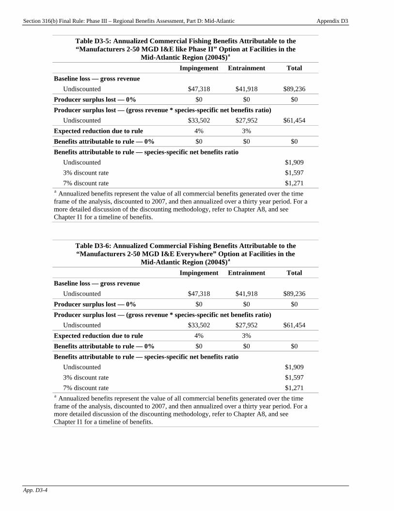
Section 316(b) Final Rule: Phase III – Regional Benefits Assessment, Part D: Mid-Atlantic Appendix D3
App. D3-4
Table D3-5: Annualized Commercial Fishing Benefits Attributable to the “Manufacturers 2-50 MGD I&E like Phase II” Option at Facilities in the
Mid-Atlantic Region (2004$)P
aP
Impingement Entrainment Total Baseline loss — gross revenue
Undiscounted $47,318 $41,918 $89,236 Producer surplus lost — 0% $0 $0 $0 Producer surplus lost — (gross revenue * species-specific net benefits ratio)
Undiscounted $33,502 $27,952 $61,454 Expected reduction due to rule 4% 3% Benefits attributable to rule — 0% $0 $0 $0 Benefits attributable to rule — species-specific net benefits ratio
Undiscounted $1,909 3% discount rate $1,597 7% discount rate $1,271
P
aP Annualized benefits represent the value of all commercial benefits generated over the time
frame of the analysis, discounted to 2007, and then annualized over a thirty year period. For a more detailed discussion of the discounting methodology, refer to Chapter A8, and see Chapter I1 for a timeline of benefits.
Table D3-6: Annualized Commercial Fishing Benefits Attributable to the “Manufacturers 2-50 MGD I&E Everywhere” Option at Facilities in the
Mid-Atlantic Region (2004$)P
aP
Impingement Entrainment Total Baseline loss — gross revenue
Undiscounted $47,318 $41,918 $89,236 Producer surplus lost — 0% $0 $0 $0 Producer surplus lost — (gross revenue * species-specific net benefits ratio)
Undiscounted $33,502 $27,952 $61,454 Expected reduction due to rule 4% 3% Benefits attributable to rule — 0% $0 $0 $0 Benefits attributable to rule — species-specific net benefits ratio
Undiscounted $1,909 3% discount rate $1,597 7% discount rate $1,271
P
aP Annualized benefits represent the value of all commercial benefits generated over the time
frame of the analysis, discounted to 2007, and then annualized over a thirty year period. For a more detailed discussion of the discounting methodology, refer to Chapter A8, and see Chapter I1 for a timeline of benefits.
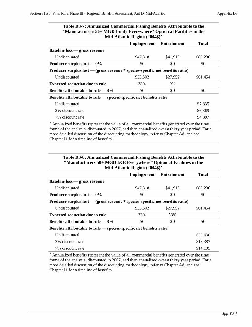
Section 316(b) Final Rule: Phase III – Regional Benefits Assessment, Part D: Mid-Atlantic Appendix D3
App. D3-5
Table D3-7: Annualized Commercial Fishing Benefits Attributable to the “Manufacturers 50+ MGD I-only Everywhere” Option at Facilities in the
Mid-Atlantic Region (2004$)P
aP
Impingement Entrainment Total Baseline loss — gross revenue
Undiscounted $47,318 $41,918 $89,236 Producer surplus lost — 0% $0 $0 $0 Producer surplus lost — (gross revenue * species-specific net benefits ratio)
Undiscounted $33,502 $27,952 $61,454 Expected reduction due to rule 23% 0% Benefits attributable to rule — 0% $0 $0 $0 Benefits attributable to rule — species-specific net benefits ratio
Undiscounted $7,835 3% discount rate $6,369 7% discount rate $4,897
P
aP Annualized benefits represent the value of all commercial benefits generated over the time
frame of the analysis, discounted to 2007, and then annualized over a thirty year period. For a more detailed discussion of the discounting methodology, refer to Chapter A8, and see Chapter I1 for a timeline of benefits.
Table D3-8: Annualized Commercial Fishing Benefits Attributable to the “Manufacturers 50+ MGD I&E Everywhere” Option at Facilities in the
Mid-Atlantic Region (2004$)P
aP
Impingement Entrainment Total Baseline loss — gross revenue
Undiscounted $47,318 $41,918 $89,236 Producer surplus lost — 0% $0 $0 $0 Producer surplus lost — (gross revenue * species-specific net benefits ratio)
Undiscounted $33,502 $27,952 $61,454 Expected reduction due to rule 23% 53% Benefits attributable to rule — 0% $0 $0 $0 Benefits attributable to rule — species-specific net benefits ratio
Undiscounted $22,630 3% discount rate $18,387 7% discount rate $14,105
P
aP Annualized benefits represent the value of all commercial benefits generated over the time
frame of the analysis, discounted to 2007, and then annualized over a thirty year period. For a more detailed discussion of the discounting methodology, refer to Chapter A8, and see Chapter I1 for a timeline of benefits.
Section 316(b) Final Rule: Phase III – Regional Benefits Assessment, Part D: Mid-Atlantic Chapter D4
D4-1
Chapter D4: Recreational Use Benefits Introduction
Chapter Contents D4-1 Benefit Transfer Approach Based on Meta-Analysis............................................... D4-1 D4-1.1 Baseline Losses and Reductions in Recreational Fishery Losses Under the Regulatory Options ................... D4-2 D4-1.2 Recreational Fishing Benefits from Eliminating Baseline I&E Losses.............................................. D4-4 D4-1.3 Recreational Fishing Benefits of the “50 MGD for All Waterbodies” Option ............................................. D4-4 D4-1.4 Recreational Fishing Benefits of the “200 MGD for All Waterbodies” Option ............................................. D4-5 D4-1.5 Recreational Fishing Benefits of the “100 MGD for Certain Waterbodies” Option ...................... D4-6 D4-2 Limitations and Uncertainty ......................... D4-6
This chapter presents the results of the recreational fishing benefits analysis for the Mid-Atlantic region. The chapter presents EPA’s estimates of baseline (i.e., current) annual recreational fishery losses from impingement and entrainment (I&E) at potentially regulated facilities in the Mid-Atlantic region and annual reductions in these losses under the regulatory options for Phase III existing facilitiesPF
1FP:
< the “50 MGD for All Waterbodies” option, < the “200 MGD for All Waterbodies” option,
and < the “100 MGD for Certain Waterbodies”
option. The chapter then presents the estimated welfare gain to Mid-Atlantic anglers from eliminating baseline recreational fishing losses from I&E and the expected benefits under the regulatory options. EPA estimated the recreational benefits of reducing and eliminating I&E losses using a benefit transfer methodology based on a meta-analysis of the marginal value of catching different species of fish. This meta-analysis is discussed in detail in Chapter A5, “Recreational Fishing Benefits Methodology.” EPA considered a wide range of policy options in developing this regulation. In addition to the regulatory options, EPA evaluated several supplemental options. Appendix D4 presents results of the recreational fishing benefits analysis for the supplemental options. For additional information on the options, please see the TDD. D4-1 Benefit Transfer Approach Based on Meta-Analysis EPA estimated the recreational welfare gain from the reduction in annual I&E losses expected under the policy options, and the welfare gain from eliminating I&E at potentially regulated facilities, using a benefit transfer approach. As discussed in Chapter A5, the Agency used a meta-analysis regression equation to estimate the marginal recreational value per additional fish caught by anglers, for different species in different regions. Since I&E at potentially regulated facilities affects a variety of species, EPA assigned each species with I&E losses to one of the general species groups used in the meta-analysis. The Agency then calculated the economic value of reducing or eliminating baseline I&E losses, for each species group, by multiplying the value per fish for that species group by the number of fish in the group that are lost in the baseline or saved under the policy options.PF
2FP
P
1P See the Introduction to this report for a description of the regulatory options.
P
2P The estimates of I&E presented in this chapter include only the fraction of impinged and entrained recreational
fish that would be caught by anglers. The total amount of I&E of recreational species is actually much higher.

Section 316(b) Final Rule: Phase III – Regional Benefits Assessment, Part D: Mid-Atlantic Chapter D4
D4-2
In general, the fit between the species with I&E losses and the species groups in the meta-analysis was good. However, EPA’s estimates of baseline I&E losses and reductions in I&E under the policy options included losses of “unidentified” species. The “unidentified” group includes fish lost indirectly through trophic transfer, as well as species for which no species information was available.PF
3FP Rather than using the meta-analysis regression to try to
predict the value per fish for an “unidentified” species, EPA assumed that per-fish values for these species can be approximated by the weighted average value per fish for all species affected by I&E in the Mid-Atlantic region.PF
4FP
D4-1.1 Baseline Losses and Reductions in Recreational Fishery Losses Under the Regulatory Options Table D4-1 presents EPA’s estimates of baseline (i.e., current) annual recreational I&E losses at potentially regulated facilities, and annual reductions in these losses under each of the regulatory options, in the Mid-Atlantic region. The table shows that total baseline losses to recreational fisheries are 108.7 thousand fish per year. In comparison, the “50 MGD for All Waterbodies” option prevents losses of 43.0 thousand fish per year, and the “200 MGD for All Waterbodies” option and the “100 MGD for Certain Waterbodies” option both prevent losses of 35.8 thousand fish per year. Of all the affected species, spot and Atlantic croaker have the highest losses in the baseline and the highest prevented losses under the regulatory options.
P
3P In addition to recreational fish that are lost because they are impinged or entrained, some recreational fish are lost
because the forage fish that they feed on are impinged or entrained, and thus removed from the food chain. These trophic transfer losses of recreational species are included in EPA’s estimates of total I&E losses. Since it is difficult to predict which recreational species would be affected by losses of forage fish, these losses are classified as “unidentified” recreational species. Also included in the “unidentified” group are losses of fish that were reported by facilities without information about their exact species.
P
4P EPA used the estimated level of baseline recreational losses for each species group as a weighting factor.

Section 316(b) Final Rule: Phase III – Regional Benefits Assessment, Part D: Mid-Atlantic Chapter D4
D4-3
Table D4-1: Baseline Recreational Fishing Losses from I&E at Potentially Regulated Phase III Facilities and Reductions in Recreational Losses Under the Regulatory Options in the
Mid-Atlantic Region Annual Reductions in Recreational Fishing Losses
(# of fish)
SpeciesP
aP
Annual Baseline Recreational Fishing
Losses (# of fish) 50 MGD All 200 MGD AllP
bP 100 MGD CWBP
bP
Bluefish 3.1 0.7 0.5 0.5 Red drum 262.8 61.5 41.1 41.1 Spotted seatrout 134.3 31.4 21.0 21.0 Striped bass 2,460.5 1,289.9 1,146.2 1,146.2 Weakfish 6,639.0 2,746.6 2,310.6 2,310.6
Total (small game) 9,499.8 4,130.1 3,519.4 3,519.4 Summer flounder 525.8 123.0 82.2 82.2 Winter flounder 288.3 130.1 111.9 111.9
Total (flatfish) 814.1 253.1 194.1 194.1 Atlantic croaker 18,023.4 8,930.1 7,843.1 7,843.1 Black drum 18.0 4.2 2.8 2.8 Searobin 14.9 3.5 2.3 2.3 Smallmouth bassP
cP 5.7 1.3 0.9 0.9
Spot 65,471.5 23,225.6 18,673.1 18,673.1 Striped mullet 1.2 0.3 0.2 0.2 White perch 374.1 129.9 103.7 103.7 WhitefishP
cP 41.9 9.8 6.6 6.6
Total (other saltwater) 83,951.0 32,304.8 26,632.9 26,632.9 Brown bullhead 203.4 47.6 31.8 31.8 Bullhead 165.6 38.7 25.9 25.9 Channel catfish 19.0 4.4 3.0 3.0 Menhaden 24.0 12.7 11.3 11.3 Sunfish 2.2 0.5 0.4 0.4 Yellow perch 21.8 6.1 4.5 4.5
Total (panfish) 436.7 110.2 77.0 77.0 Total (unidentified) 13,952.6 6,250.7 5,365.8 5,365.8 Total (all species) 108,654.2 43,049.0 35,789.2 35,789.2 P
aP EPA assigned each species with I&E losses to one of the species groups used in the meta-analysis. The “other
saltwater” group includes bottomfish and other miscellaneous species. The “unidentified” group includes fish lost indirectly through trophic transfer and fish reported lost without information about their species. P
bP Annual reductions in recreational I&E losses are the same in the Mid-Atlantic region for the “200 MGD for All
Waterbodies” and “100 MGD for Certain Waterbodies” options. P
cP The “other saltwater” species group includes two freshwater species, smallmouth bass and whitefish, which can be
found in estuarine environments. Source: U.S. EPA analysis for this report.
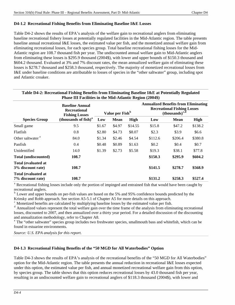
Section 316(b) Final Rule: Phase III – Regional Benefits Assessment, Part D: Mid-Atlantic Chapter D4
D4-4
D4-1.2 Recreational Fishing Benefits from Eliminating Baseline I&E Losses Table D4-2 shows the results of EPA’s analysis of the welfare gain to recreational anglers from eliminating baseline recreational fishery losses at potentially regulated facilities in the Mid-Atlantic region. The table presents baseline annual recreational I&E losses, the estimated value per fish, and the monetized annual welfare gain from eliminating recreational losses, for each species group. Total baseline recreational fishing losses for the Mid-Atlantic region are 108.7 thousand fish per year. The undiscounted annual welfare gain to Mid-Atlantic anglers from eliminating these losses is $295.9 thousand (2004$), with lower and upper bounds of $150.3 thousand and $604.2 thousand. Evaluated at 3% and 7% discount rates, the mean annualized welfare gain of eliminating these losses is $278.7 thousand and $258.3 thousand, respectively. The majority of monetized recreational losses from I&E under baseline conditions are attributable to losses of species in the “other saltwater” group, including spot and Atlantic croaker.
Table D4-2: Recreational Fishing Benefits from Eliminating Baseline I&E at Potentially Regulated Phase III Facilities in the Mid-Atlantic Region (2004$)
Value per FishP
bP
Annualized Benefits from Eliminating Recreational Fishing Losses
(thousands)P
c,dP
Species Group
Baseline Annual Recreational
Fishing Losses (thousands of fish)P
aP Low Mean High Low Mean High
Small game 9.5 $1.67 $4.97 $14.55 $15.8 $47.2 $138.2 Flatfish 0.8 $2.80 $4.73 $8.07 $2.3 $3.9 $6.6 Other saltwaterP
eP 84.0 $1.34 $2.46 $4.54 $112.6 $206.4 $380.8
Panfish 0.4 $0.48 $0.89 $1.63 $0.2 $0.4 $0.7 Unidentified 14.0 $1.39 $2.73 $5.58 $19.3 $38.1 $77.8 Total (undiscounted) 108.7 $150.3 $295.9 $604.2 Total (evaluated at 3% discount rate) 108.7 $141.5 $278.7 $568.9 Total (evaluated at 7% discount rate) 108.7 $131.2 $258.3 $527.4 P
aP Recreational fishing losses include only the portion of impinged and entrained fish that would have been caught by
recreational anglers. P
bP Lower and upper bounds on per-fish values are based on the 5% and 95% confidence bounds predicted by the
Krinsky and Robb approach. See section A5-5.1 of Chapter A5 for more details on this approach. P
cP Monetized benefits are calculated by multiplying baseline losses by the estimated value per fish.
P
dP Annualized values represent the total welfare gain over the time frame of the analysis from eliminating recreational
losses, discounted to 2007, and then annualized over a thirty year period. For a detailed discussion of the discounting and annualization methodology, refer to Chapter A8. P
eP The “other saltwater” species group includes two freshwater species, smallmouth bass and whitefish, which can be
found in estuarine environments. Source: U.S. EPA analysis for this report. D4-1.3 Recreational Fishing Benefits of the “50 MGD for All Waterbodies” Option Table D4-3 shows the results of EPA’s analysis of the recreational benefits of the “50 MGD for All Waterbodies” option for the Mid-Atlantic region. The table presents the annual reduction in recreational I&E losses expected under this option, the estimated value per fish, and annual monetized recreational welfare gain from this option, by species group. The table shows that this option reduces recreational losses by 43.0 thousand fish per year, resulting in an undiscounted welfare gain to recreational anglers of $118.3 thousand (2004$), with lower and

Section 316(b) Final Rule: Phase III – Regional Benefits Assessment, Part D: Mid-Atlantic Chapter D4
D4-5
upper bounds of $59.6 thousand and $243.7 thousand. Evaluated at 3% and 7% discount rates, the mean annualized welfare gain from this reduction in recreational losses is $96.1 thousand and $73.7 thousand, respectively. The majority of benefits result from reduced losses of species in the “other saltwater” group, including spot and Atlantic croaker.
Table D4-3: Recreational Fishing Benefits of the “50 MGD for All Waterbodies” Option in the Mid-Atlantic Region (2004$)
Value per FishP
bP
Annualized Recreational Fishing Benefits (thousands)P
c,dP
Species Group
Annual Reduction in Recreational Fishing Losses
(thousands of fish)P
aP Low Mean High Low Mean High
Small game 4.1 $1.67 $4.97 $14.55 $6.9 $20.5 $60.1 Flatfish 0.3 $2.80 $4.73 $8.07 $0.7 $1.2 $2.0 Other saltwaterP
eP 32.3 $1.34 $2.46 $4.54 $43.3 $79.4 $146.5
Panfish 0.1 $0.48 $0.89 $1.63 $0.1 $0.1 $0.2 Unidentified 6.3 $1.39 $2.73 $5.58 $8.7 $17.1 $34.9 Total (undiscounted) 43.0 $59.6 $118.3 $243.7 Total (evaluated at 3% discount rate) 43.0 $48.5 $96.1 $198.0 Total (evaluated at 7% discount rate) 43.0 $37.2 $73.7 $151.9 P
aP Recreational fishing losses include only the portion of impinged and entrained fish that would have been caught by
recreational anglers. P
bP Lower and upper bounds on per-fish values are based on the 5% and 95% confidence bounds predicted by the
Krinsky and Robb approach. See section A5-5.1 of Chapter A5 for more details on this approach. P
cP Monetized benefits are calculated by multiplying the annual reduction in recreational losses by the estimated value
per fish. P
dP Annualized benefits represent the value of all recreational benefits generated over the time frame of the analysis,
discounted to 2007, and then annualized over a thirty year period. For a detailed discussion of the discounting and annualization methodology, refer to Chapter A8. P
eP The “other saltwater” species group includes two freshwater species, smallmouth bass and whitefish, which can be
found in estuarine environments. Source: U.S. EPA analysis for this report.
D4-1.4 Recreational Fishing Benefits of the “200 MGD for All Waterbodies” Option Table D4-4 shows the results of EPA’s analysis of the recreational benefits of the “200 MGD for All Waterbodies” option for the Mid-Atlantic region. The table presents the annual reduction in recreational I&E losses expected under this option, the estimated value per fish, and annual monetized recreational welfare gain from this option, by species group. The table shows that this option reduces recreational losses by 35.8 thousand fish per year, resulting in an undiscounted welfare gain to recreational anglers of $98.6 thousand (2004$), with lower and upper bounds of $49.6 thousand and $203.6 thousand. Evaluated at 3% and 7% discount rates, the mean annualized welfare gain from this reduction in recreational losses is $79.5 thousand and $60.4 thousand, respectively. The majority of benefits result from reduced losses of species in the “other saltwater” group, including spot and Atlantic croaker.
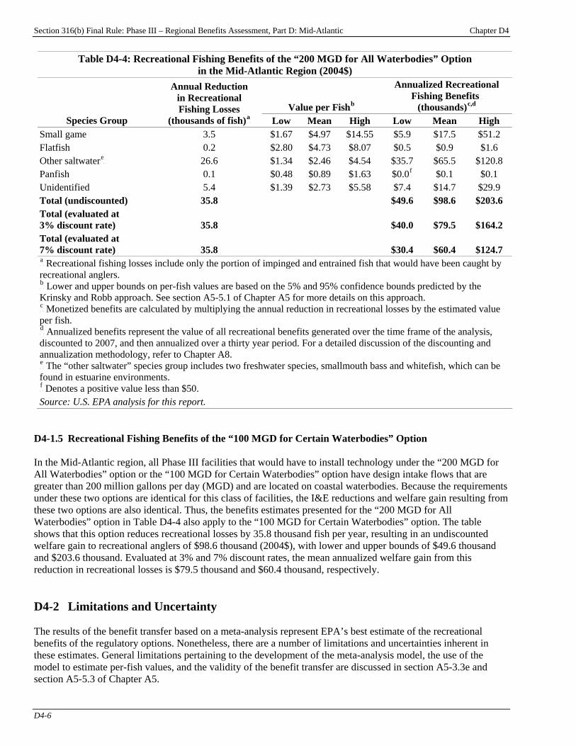
Section 316(b) Final Rule: Phase III – Regional Benefits Assessment, Part D: Mid-Atlantic Chapter D4
D4-6
Table D4-4: Recreational Fishing Benefits of the “200 MGD for All Waterbodies” Option in the Mid-Atlantic Region (2004$)
Value per FishP
bP
Annualized Recreational Fishing Benefits P
P(thousands)P
c,dP
Species Group
Annual Reduction in Recreational Fishing Losses
(thousands of fish)P
aP Low Mean High Low Mean High
Small game 3.5 $1.67 $4.97 $14.55 $5.9 $17.5 $51.2 Flatfish 0.2 $2.80 $4.73 $8.07 $0.5 $0.9 $1.6 Other saltwaterP
eP 26.6 $1.34 $2.46 $4.54 $35.7 $65.5 $120.8
Panfish 0.1 $0.48 $0.89 $1.63 $0.0P
fP $0.1 $0.1
Unidentified 5.4 $1.39 $2.73 $5.58 $7.4 $14.7 $29.9 Total (undiscounted) 35.8 $49.6 $98.6 $203.6 Total (evaluated at 3% discount rate) 35.8 $40.0 $79.5 $164.2 Total (evaluated at 7% discount rate) 35.8 $30.4 $60.4 $124.7 P
aP Recreational fishing losses include only the portion of impinged and entrained fish that would have been caught by
recreational anglers. P
bP Lower and upper bounds on per-fish values are based on the 5% and 95% confidence bounds predicted by the
Krinsky and Robb approach. See section A5-5.1 of Chapter A5 for more details on this approach. P
cP Monetized benefits are calculated by multiplying the annual reduction in recreational losses by the estimated value
per fish. P
dP Annualized benefits represent the value of all recreational benefits generated over the time frame of the analysis,
discounted to 2007, and then annualized over a thirty year period. For a detailed discussion of the discounting and annualization methodology, refer to Chapter A8. P
eP The “other saltwater” species group includes two freshwater species, smallmouth bass and whitefish, which can be
found in estuarine environments. P
fP Denotes a positive value less than $50.
Source: U.S. EPA analysis for this report. D4-1.5 Recreational Fishing Benefits of the “100 MGD for Certain Waterbodies” Option In the Mid-Atlantic region, all Phase III facilities that would have to install technology under the “200 MGD for All Waterbodies” option or the “100 MGD for Certain Waterbodies” option have design intake flows that are greater than 200 million gallons per day (MGD) and are located on coastal waterbodies. Because the requirements under these two options are identical for this class of facilities, the I&E reductions and welfare gain resulting from these two options are also identical. Thus, the benefits estimates presented for the “200 MGD for All Waterbodies” option in Table D4-4 also apply to the “100 MGD for Certain Waterbodies” option. The table shows that this option reduces recreational losses by 35.8 thousand fish per year, resulting in an undiscounted welfare gain to recreational anglers of $98.6 thousand (2004$), with lower and upper bounds of $49.6 thousand and $203.6 thousand. Evaluated at 3% and 7% discount rates, the mean annualized welfare gain from this reduction in recreational losses is $79.5 thousand and $60.4 thousand, respectively. D4-2 Limitations and Uncertainty The results of the benefit transfer based on a meta-analysis represent EPA’s best estimate of the recreational benefits of the regulatory options. Nonetheless, there are a number of limitations and uncertainties inherent in these estimates. General limitations pertaining to the development of the meta-analysis model, the use of the model to estimate per-fish values, and the validity of the benefit transfer are discussed in section A5-3.3e and section A5-5.3 of Chapter A5.
Section 316(b) Final Rule: Phase III – Regional Benefits Assessment, Part D: Mid-Atlantic Appendix D4
App. D4-1
Appendix D4: Recreational Use Benefits Under Supplemental Policy Options
Introduction
Appendix Contents D4-1 Recreational Fishing Benefits of the Supplemental Options ...................................D4-1 D4-1.1 Estimated Reductions in Recreational Fishing Losses Under the Supplemental Options.....D4-1 D4-1.2 Recreational Fishing Benefits of the Supplemental Options ...............D4-4 D4-2 Comparison of Recreational Fishing Benefits by Option ......................................D4-10
Chapter D4 presents EPA’s estimates of the recreational benefits of the regulatory options for the section 316(b) rule for Phase III facilities in the Mid-Atlantic region. To facilitate comparisons among the options, this appendix presents estimates of the recreational fishing benefits of several supplemental options that EPA evaluated in preparation for this rule:
< “Electric Generators 2-50 MGD I-only Everywhere” option;
< “Electric Generators 2-50 MGD I&E like Phase II” option; < “Electric Generators 2-50 MGD I&E Everywhere” option; < “Manufacturers 2-50 MGD I-only Everywhere” option; < “Manufacturers 2-50 MGD I&E like Phase II” option; < “Manufacturers 2-50 MGD I&E Everywhere” option; < “Manufacturers 50+ MGD I-only Everywhere” option; and < “Manufacturers 50+ MGD I&E Everywhere” option.
Recreational fishing benefits presented in this chapter were estimated using the benefit transfer approach discussed in Chapter D4 and in Chapter A5, “Recreational Fishing Benefits Methodology.” D4-1 Recreational Fishing Benefits of the Supplemental Options D4-1.1 Estimated Reductions in Recreational Fishing Losses Under the Supplemental Options Table D4-1 presents EPA’s estimates of the annual reduction in baseline (i.e., current) recreational fishing losses from impingement and entrainment (I&E) in the Mid-Atlantic region under the supplemental options. For additional information on the options, please see the TDD.
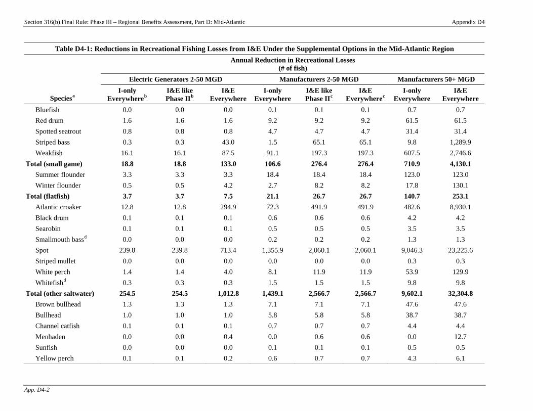
Section 316(b) Final Rule: Phase III – Regional Benefits Assessment, Part D: Mid-Atlantic Appendix D4
App. D4-2
Table D4-1: Reductions in Recreational Fishing Losses from I&E Under the Supplemental Options in the Mid-Atlantic Region Annual Reduction in Recreational Losses
(# of fish) Electric Generators 2-50 MGD Manufacturers 2-50 MGD Manufacturers 50+ MGD
SpeciesP
aP
I-only EverywhereP
bP
I&E like Phase IIP
bP
I&E Everywhere
I-only Everywhere
I&E like Phase IIP
cP
I&E EverywhereP
cP
I-only Everywhere
I&E Everywhere
Bluefish 0.0 0.0 0.0 0.1 0.1 0.1 0.7 0.7 Red drum 1.6 1.6 1.6 9.2 9.2 9.2 61.5 61.5 Spotted seatrout 0.8 0.8 0.8 4.7 4.7 4.7 31.4 31.4 Striped bass 0.3 0.3 43.0 1.5 65.1 65.1 9.8 1,289.9 Weakfish 16.1 16.1 87.5 91.1 197.3 197.3 607.5 2,746.6
Total (small game) 18.8 18.8 133.0 106.6 276.4 276.4 710.9 4,130.1 Summer flounder 3.3 3.3 3.3 18.4 18.4 18.4 123.0 123.0 Winter flounder 0.5 0.5 4.2 2.7 8.2 8.2 17.8 130.1
Total (flatfish) 3.7 3.7 7.5 21.1 26.7 26.7 140.7 253.1 Atlantic croaker 12.8 12.8 294.9 72.3 491.9 491.9 482.6 8,930.1 Black drum 0.1 0.1 0.1 0.6 0.6 0.6 4.2 4.2 Searobin 0.1 0.1 0.1 0.5 0.5 0.5 3.5 3.5 Smallmouth bassP
dP 0.0 0.0 0.0 0.2 0.2 0.2 1.3 1.3
Spot 239.8 239.8 713.4 1,355.9 2,060.1 2,060.1 9,046.3 23,225.6 Striped mullet 0.0 0.0 0.0 0.0 0.0 0.0 0.3 0.3 White perch 1.4 1.4 4.0 8.1 11.9 11.9 53.9 129.9 WhitefishP
dP 0.3 0.3 0.3 1.5 1.5 1.5 9.8 9.8
Total (other saltwater) 254.5 254.5 1,012.8 1,439.1 2,566.7 2,566.7 9,602.1 32,304.8 Brown bullhead 1.3 1.3 1.3 7.1 7.1 7.1 47.6 47.6 Bullhead 1.0 1.0 1.0 5.8 5.8 5.8 38.7 38.7 Channel catfish 0.1 0.1 0.1 0.7 0.7 0.7 4.4 4.4 Menhaden 0.0 0.0 0.4 0.0 0.6 0.6 0.0 12.7 Sunfish 0.0 0.0 0.0 0.1 0.1 0.1 0.5 0.5 Yellow perch 0.1 0.1 0.2 0.6 0.7 0.7 4.3 6.1

316(b) Final Rule: Phase III – Regional Benefits Assessment, Part D: Mid-Atlantic Appendix D4
App. D4-3
2.5 2.5 3.0 14.3 15.1 15.1 95.7 110.2 23.8 23.8 202.6 134.6 400.4 400.4 898.0 6,250.7
303.5 303.5 1,358.9 1,715.7 3,285.2 3,285.2 11,447.4 43,049.0
Table D4-1: Reductions in Recreational Fishing Losses from I&E Under the Supplemental Options in the Mid-Atlantic Region Annual Reduction in Recreational Losses
(# of fish) Electric Generators 2-50 MGD Manufacturers 2-50 MGD Manufacturers 50+ MGD
SpeciesP
aP
I-only EverywhereP
bP
I&E like Phase IIP
bP
I&E Everywhere
I-only Everywhere
I&E like Phase IIP
cP
I&E EverywhereP
cP
I-only Everywhere
I&E Everywhere
Total (panfish)
P
aP EPA assigned each species with I&E losses to one of the species groups used in the meta-analysis. The “other saltwater” group includes bottomfish and other
miscellaneous species. The “unidentified” group includes fish lost indirectly through trophic transfer and fish reported lost without information about their species. P
bP Annual reductions in recreational I&E losses are the same in the Mid-Atlantic region for the “Electric Generators 2-50 MGD I-only Everywhere” and “Electric
Generators 2-50 MGD I&E like Phase II” options. P
cP Annual reductions in recreational I&E losses are the same in the Mid-Atlantic region for the “Manufacturers 2-50 MGD I&E like Phase II” and “Manufacturers
2-50 MGD I&E Everywhere” options. P
dP The “other saltwater” species group includes two freshwater species, smallmouth bass and whitefish, which can be found in estuarine environments.
Source: U.S. EPA analysis for this report.
Total (unidentified) Total (all species)
Section
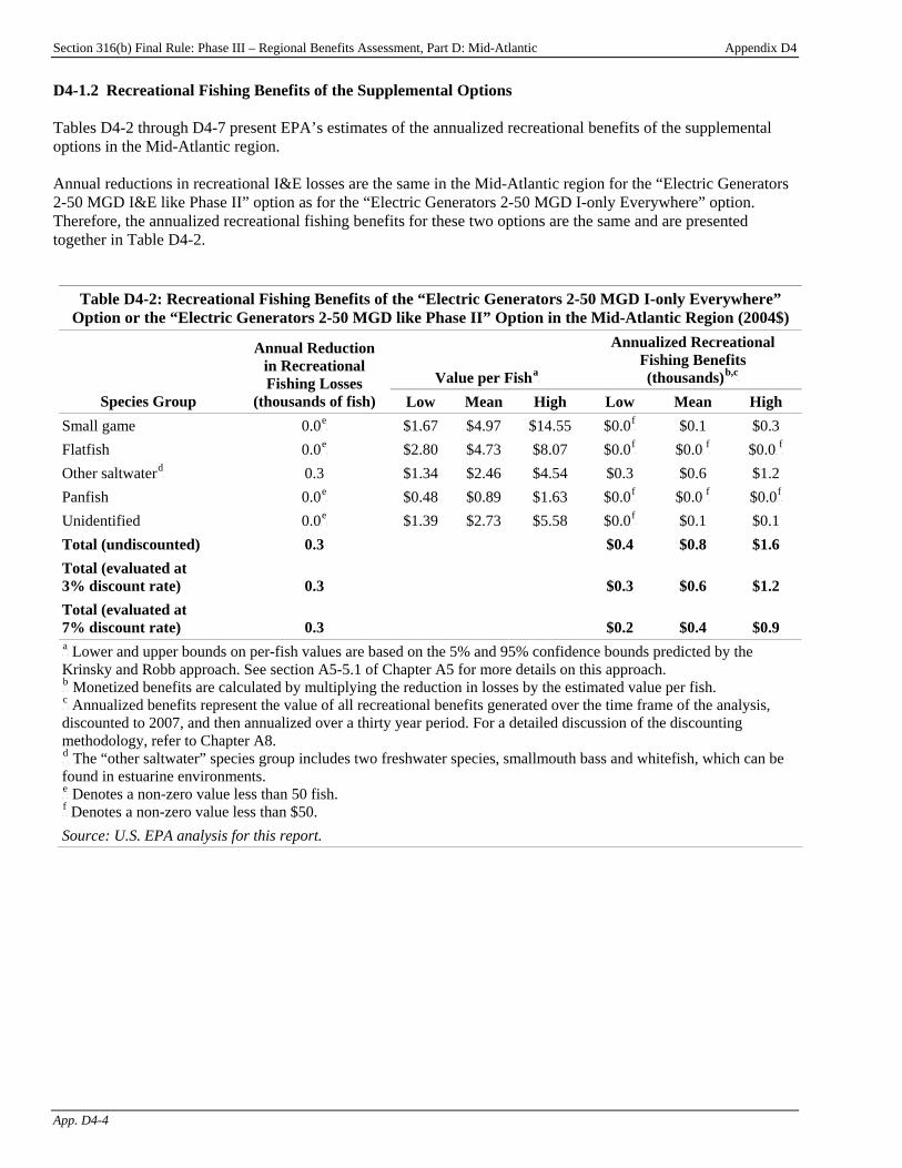
Section 316(b) Final Rule: Phase III – Regional Benefits Assessment, Part D: Mid-Atlantic Appendix D4
App. D4-4
D4-1.2 Recreational Fishing Benefits of the Supplemental Options Tables D4-2 through D4-7 present EPA’s estimates of the annualized recreational benefits of the supplemental options in the Mid-Atlantic region. Annual reductions in recreational I&E losses are the same in the Mid-Atlantic region for the “Electric Generators 2-50 MGD I&E like Phase II” option as for the “Electric Generators 2-50 MGD I-only Everywhere” option. Therefore, the annualized recreational fishing benefits for these two options are the same and are presented together in Table D4-2.
Table D4-2: Recreational Fishing Benefits of the “Electric Generators 2-50 MGD I-only Everywhere” Option or the “Electric Generators 2-50 MGD like Phase II” Option in the Mid-Atlantic Region (2004$)
Value per FishP
aP
Annualized Recreational Fishing Benefits (thousands)P
b,cP
Species Group
Annual Reduction in Recreational Fishing Losses
(thousands of fish) Low Mean High Low Mean High Small game 0.0P
eP $1.67 $4.97 $14.55 $0.0P
fP $0.1 $0.3
Flatfish 0.0P
eP $2.80 $4.73 $8.07 $0.0P
fP $0.0P
fP $0.0P
fP
Other saltwaterP
dP 0.3 $1.34 $2.46 $4.54 $0.3 $0.6 $1.2
Panfish 0.0P
eP $0.48 $0.89 $1.63 $0.0P
fP $0.0P
fP $0.0P
fP
Unidentified 0.0P
eP $1.39 $2.73 $5.58 $0.0P
fP $0.1 $0.1
Total (undiscounted) 0.3 $0.4 $0.8 $1.6 Total (evaluated at 3% discount rate) 0.3 $0.3 $0.6 $1.2 Total (evaluated at 7% discount rate) 0.3 $0.2 $0.4 $0.9 P
aP Lower and upper bounds on per-fish values are based on the 5% and 95% confidence bounds predicted by the
Krinsky and Robb approach. See section A5-5.1 of Chapter A5 for more details on this approach. P
bP Monetized benefits are calculated by multiplying the reduction in losses by the estimated value per fish.
P
cP Annualized benefits represent the value of all recreational benefits generated over the time frame of the analysis,
discounted to 2007, and then annualized over a thirty year period. For a detailed discussion of the discounting methodology, refer to Chapter A8. P
dP The “other saltwater” species group includes two freshwater species, smallmouth bass and whitefish, which can be
found in estuarine environments. P
eP Denotes a non-zero value less than 50 fish.
P
fP Denotes a non-zero value less than $50.
Source: U.S. EPA analysis for this report.
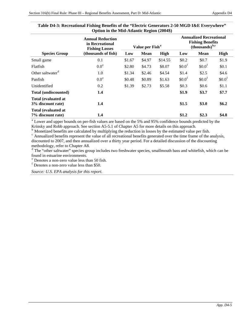
Section 316(b) Final Rule: Phase III – Regional Benefits Assessment, Part D: Mid-Atlantic Appendix D4
App. D4-5
Table D4-3: Recreational Fishing Benefits of the “Electric Generators 2-50 MGD I&E Everywhere” Option in the Mid-Atlantic Region (2004$)
Value per FishP
aP
Annualized Recreational Fishing Benefits (thousands)P
b,cP
Species Group
Annual Reduction in Recreational Fishing Losses
(thousands of fish) Low Mean High Low Mean High Small game 0.1 $1.67 $4.97 $14.55 $0.2 $0.7 $1.9 Flatfish 0.0P
eP $2.80 $4.73 $8.07 $0.0P
fP $0.0P
fP $0.1
Other saltwaterP
dP 1.0 $1.34 $2.46 $4.54 $1.4 $2.5 $4.6
Panfish 0.0P
eP $0.48 $0.89 $1.63 $0.0P
fP $0.0P
fP $0.0P
fP
Unidentified 0.2 $1.39 $2.73 $5.58 $0.3 $0.6 $1.1 Total (undiscounted) 1.4 $1.9 $3.7 $7.7 Total (evaluated at 3% discount rate) 1.4 $1.5 $3.0 $6.2 Total (evaluated at 7% discount rate) 1.4 $1.2 $2.3 $4.8 P
aP Lower and upper bounds on per-fish values are based on the 5% and 95% confidence bounds predicted by the
Krinsky and Robb approach. See section A5-5.1 of Chapter A5 for more details on this approach. P
bP Monetized benefits are calculated by multiplying the reduction in losses by the estimated value per fish.
P
cP Annualized benefits represent the value of all recreational benefits generated over the time frame of the analysis,
discounted to 2007, and then annualized over a thirty year period. For a detailed discussion of the discounting methodology, refer to Chapter A8. P
dP The “other saltwater” species group includes two freshwater species, smallmouth bass and whitefish, which can be
found in estuarine environments. P
eP Denotes a non-zero value less than 50 fish.
P
fP Denotes a non-zero value less than $50.
Source: U.S. EPA analysis for this report.
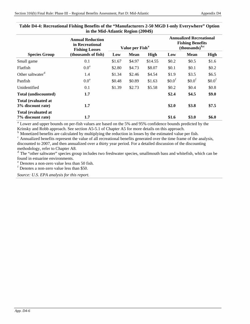
Section 316(b) Final Rule: Phase III – Regional Benefits Assessment, Part D: Mid-Atlantic Appendix D4
App. D4-6
Table D4-4: Recreational Fishing Benefits of the “Manufacturers 2-50 MGD I-only Everywhere” Option in the Mid-Atlantic Region (2004$)
Value per FishP
aP
Annualized Recreational Fishing Benefits (thousands)P
b,cP
Species Group
Annual Reduction in Recreational Fishing Losses
(thousands of fish) Low Mean High Low Mean High Small game 0.1 $1.67 $4.97 $14.55 $0.2 $0.5 $1.6 Flatfish 0.0P
eP $2.80 $4.73 $8.07 $0.1 $0.1 $0.2
Other saltwaterP
dP 1.4 $1.34 $2.46 $4.54 $1.9 $3.5 $6.5
Panfish 0.0P
eP $0.48 $0.89 $1.63 $0.0P
fP $0.0P
fP $0.0P
fP
Unidentified 0.1 $1.39 $2.73 $5.58 $0.2 $0.4 $0.8 Total (undiscounted) 1.7 $2.4 $4.5 $9.0 Total (evaluated at 3% discount rate) 1.7 $2.0 $3.8 $7.5 Total (evaluated at 7% discount rate) 1.7 $1.6 $3.0 $6.0 P
aP Lower and upper bounds on per-fish values are based on the 5% and 95% confidence bounds predicted by the
Krinsky and Robb approach. See section A5-5.1 of Chapter A5 for more details on this approach. P
bP Monetized benefits are calculated by multiplying the reduction in losses by the estimated value per fish.
P
cP Annualized benefits represent the value of all recreational benefits generated over the time frame of the analysis,
discounted to 2007, and then annualized over a thirty year period. For a detailed discussion of the discounting methodology, refer to Chapter A8. P
dP The “other saltwater” species group includes two freshwater species, smallmouth bass and whitefish, which can be
found in estuarine environments. P
eP Denotes a non-zero value less than 50 fish.
P
fP Denotes a non-zero value less than $50.
Source: U.S. EPA analysis for this report.

Section 316(b) Final Rule: Phase III – Regional Benefits Assessment, Part D: Mid-Atlantic Appendix D4
App. D4-7
Annual reductions in recreational I&E losses are the same in the Mid-Atlantic region for the “Manufacturers 2-50 MGD I&E Everywhere” option as for the “Manufacturers 2-50 MGD I&E like Phase II” option. Therefore, the annualized recreational fishing benefits for these two options are the same, and are presented together in Table D4-5.
Table D4-5: Recreational Fishing Benefits of the “Manufacturers 2-50 MGD I&E like Phase II” Option and the “Manufacturers 2-50 MGD I&E Everywhere” Option in the Mid-Atlantic Region (2004$)
Value per FishP
aP
Annualized Recreational Fishing Benefits (thousands)P
b,cP
Species Group
Annual Reduction in Recreational Fishing Losses
(thousands of fish) Low Mean High Low Mean High Small game 0.3 $1.67 $4.97 $14.55 $0.5 $1.4 $4.0 Flatfish 0.0P
eP $2.80 $4.73 $8.07 $0.1 $0.1 $0.2
Other saltwaterP
dP 2.6 $1.34 $2.46 $4.54 $3.4 $6.3 $11.6
Panfish 0.0P
eP $0.48 $0.89 $1.63 $0.0P
fP $0.0P
fP $0.0P
fP
Unidentified 0.4 $1.39 $2.73 $5.58 $0.6 $1.1 $2.2 Total (undiscounted) 3.3 $4.5 $8.9 $18.1 Total (evaluated at 3% discount rate) 3.3 $3.8 $7.5 $15.2 Total (evaluated at 7% discount rate) 3.3 $3.0 $5.9 $12.1 P
aP Lower and upper bounds on per-fish values are based on the 5% and 95% confidence bounds predicted by the
Krinsky and Robb approach. See section A5-5.1 of Chapter A5 for more details on this approach. P
bP Monetized benefits are calculated by multiplying the reduction in losses by the estimated value per fish.
P
cP Annualized benefits represent the value of all recreational benefits generated over the time frame of the analysis,
discounted to 2007, and then annualized over a thirty year period. For a detailed discussion of the discounting methodology, refer to Chapter A8. P
dP The “other saltwater” species group includes two freshwater species, smallmouth bass and whitefish, which can be
found in estuarine environments. P
eP Denotes a non-zero value less than 50 fish.
P
fP Denotes a non-zero value less than $50.
Source: U.S. EPA analysis for this report.

Section 316(b) Final Rule: Phase III – Regional Benefits Assessment, Part D: Mid-Atlantic Appendix D4
App. D4-8
Table D4-6: Recreational Fishing Benefits of the “Manufacturers 50+ MGD I-only Everywhere” Option in the Mid-Atlantic Region (2004$)
Value per FishP
aP
Annualized Recreational Fishing Benefits (thousands)P
b,cP
Species Group
Annual Reduction in Recreational Fishing Losses
(thousands of fish) Low Mean High Low Mean High Small game 0.7 $1.67 $4.97 $14.55 $1.2 $3.5 $10.3 Flatfish 0.1 $2.80 $4.73 $8.07 $0.4 $0.7 $1.1 Other saltwaterP
dP 9.6 $1.34 $2.46 $4.54 $12.9 $23.6 $43.6
Panfish 0.1 $0.48 $0.89 $1.63 $0.0P
eP $0.1 $0.2
Unidentified 0.9 $1.39 $2.73 $5.58 $1.2 $2.5 $5.0 Total (undiscounted) 11.4 $15.7 $30.3 $60.2 Total (evaluated at 3% discount rate) 11.4 $12.8 $24.7 $48.9 Total (evaluated at 7% discount rate) 11.4 $9.8 $19.0 $37.6 P
aP Lower and upper bounds on per-fish values are based on the 5% and 95% confidence bounds predicted by the
Krinsky and Robb approach. See section A5-5.1 of Chapter A5 for more details on this approach. P
bP Monetized benefits are calculated by multiplying the reduction in losses by the estimated value per fish.
P
cP Annualized benefits represent the value of all recreational benefits generated over the time frame of the analysis,
discounted to 2007, and then annualized over a thirty year period. For a detailed discussion of the discounting methodology, refer to Chapter A8. P
dP The “other saltwater” species group includes two freshwater species, smallmouth bass and whitefish, which can be
found in estuarine environments. P
eP Denotes a non-zero value less than $50.
Source: U.S. EPA analysis for this report.
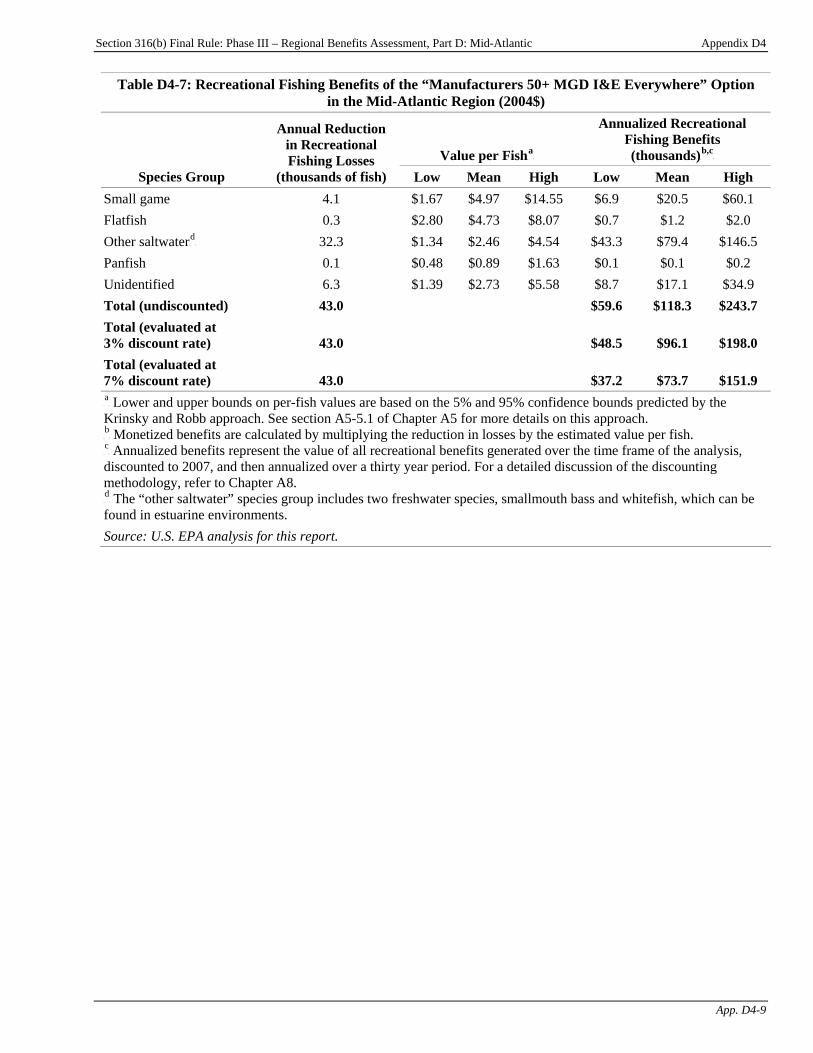
Section 316(b) Final Rule: Phase III – Regional Benefits Assessment, Part D: Mid-Atlantic Appendix D4
App. D4-9
Table D4-7: Recreational Fishing Benefits of the “Manufacturers 50+ MGD I&E Everywhere” Option in the Mid-Atlantic Region (2004$)
Value per FishP
aP
Annualized Recreational Fishing Benefits (thousands)P
b,cP
Species Group
Annual Reduction in Recreational Fishing Losses
(thousands of fish) Low Mean High Low Mean High Small game 4.1 $1.67 $4.97 $14.55 $6.9 $20.5 $60.1 Flatfish 0.3 $2.80 $4.73 $8.07 $0.7 $1.2 $2.0 Other saltwaterP
dP 32.3 $1.34 $2.46 $4.54 $43.3 $79.4 $146.5
Panfish 0.1 $0.48 $0.89 $1.63 $0.1 $0.1 $0.2 Unidentified 6.3 $1.39 $2.73 $5.58 $8.7 $17.1 $34.9 Total (undiscounted) 43.0 $59.6 $118.3 $243.7 Total (evaluated at 3% discount rate) 43.0 $48.5 $96.1 $198.0 Total (evaluated at 7% discount rate) 43.0 $37.2 $73.7 $151.9 P
aP Lower and upper bounds on per-fish values are based on the 5% and 95% confidence bounds predicted by the
Krinsky and Robb approach. See section A5-5.1 of Chapter A5 for more details on this approach. P
bP Monetized benefits are calculated by multiplying the reduction in losses by the estimated value per fish.
P
cP Annualized benefits represent the value of all recreational benefits generated over the time frame of the analysis,
discounted to 2007, and then annualized over a thirty year period. For a detailed discussion of the discounting methodology, refer to Chapter A8. P
dP The “other saltwater” species group includes two freshwater species, smallmouth bass and whitefish, which can be
found in estuarine environments. Source: U.S. EPA analysis for this report.
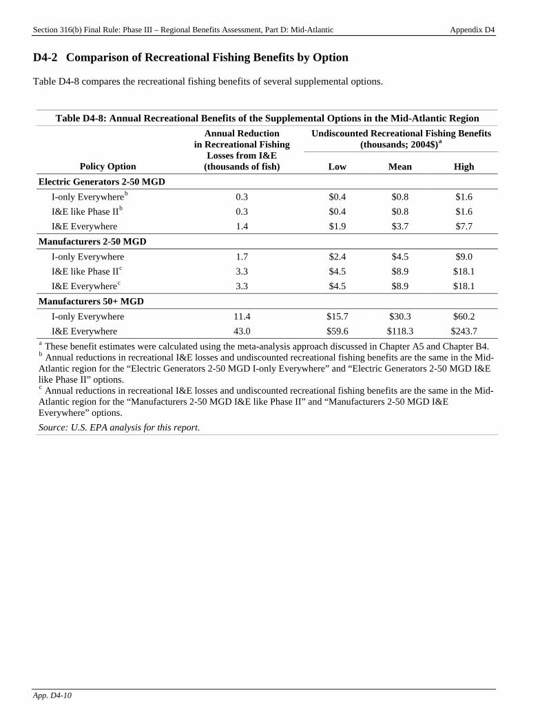
Section 316(b) Final Rule: Phase III – Regional Benefits Assessment, Part D: Mid-Atlantic Appendix D4
App. D4-10
D4-2 Comparison of Recreational Fishing Benefits by Option Table D4-8 compares the recreational fishing benefits of several supplemental options.
Table D4-8: Annual Recreational Benefits of the Supplemental Options in the Mid-Atlantic Region Undiscounted Recreational Fishing Benefits
(thousands; 2004$)P
aP
Policy Option
Annual Reduction in Recreational Fishing
Losses from I&E (thousands of fish) Low Mean High
Electric Generators 2-50 MGD I-only EverywhereP
bP 0.3 $0.4 $0.8 $1.6
I&E like Phase IIP
bP 0.3 $0.4 $0.8 $1.6
I&E Everywhere 1.4 $1.9 $3.7 $7.7 Manufacturers 2-50 MGD
I-only Everywhere 1.7 $2.4 $4.5 $9.0 I&E like Phase IIP
cP 3.3 $4.5 $8.9 $18.1
I&E EverywhereP
cP 3.3 $4.5 $8.9 $18.1
Manufacturers 50+ MGD I-only Everywhere 11.4 $15.7 $30.3 $60.2 I&E Everywhere 43.0 $59.6 $118.3 $243.7
P
aP These benefit estimates were calculated using the meta-analysis approach discussed in Chapter A5 and Chapter B4.
P
bP Annual reductions in recreational I&E losses and undiscounted recreational fishing benefits are the same in the Mid-
Atlantic region for the “Electric Generators 2-50 MGD I-only Everywhere” and “Electric Generators 2-50 MGD I&E like Phase II” options. P
cP Annual reductions in recreational I&E losses and undiscounted recreational fishing benefits are the same in the Mid-
Atlantic region for the “Manufacturers 2-50 MGD I&E like Phase II” and “Manufacturers 2-50 MGD I&E Everywhere” options. Source: U.S. EPA analysis for this report.
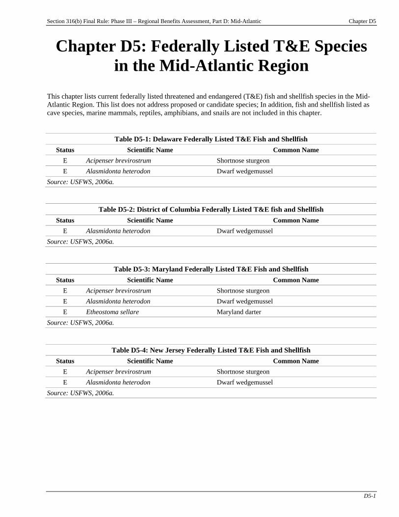
Section 316(b) Final Rule: Phase III – Regional Benefits Assessment, Part D: Mid-Atlantic Chapter D5
D5-1
Chapter D5: Federally Listed T&E Species in the Mid-Atlantic Region
This chapter lists current federally listed threatened and endangered (T&E) fish and shellfish species in the Mid-Atlantic Region. This list does not address proposed or candidate species; In addition, fish and shellfish listed as cave species, marine mammals, reptiles, amphibians, and snails are not included in this chapter.
Table D5-1: Delaware Federally Listed T&E Fish and Shellfish Status Scientific Name Common Name
E Acipenser brevirostrum Shortnose sturgeon E Alasmidonta heterodon Dwarf wedgemussel
Source: USFWS, 2006a.
Table D5-2: District of Columbia Federally Listed T&E fish and Shellfish Status Scientific Name Common Name
E Alasmidonta heterodon Dwarf wedgemussel Source: USFWS, 2006a.
Table D5-3: Maryland Federally Listed T&E Fish and Shellfish Status Scientific Name Common Name
E Acipenser brevirostrum Shortnose sturgeon E Alasmidonta heterodon Dwarf wedgemussel E Etheostoma sellare Maryland darter
Source: USFWS, 2006a.
Table D5-4: New Jersey Federally Listed T&E Fish and Shellfish Status Scientific Name Common Name
E Acipenser brevirostrum Shortnose sturgeon E Alasmidonta heterodon Dwarf wedgemussel
Source: USFWS, 2006a.
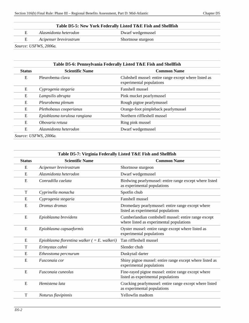
Section 316(b) Final Rule: Phase III – Regional Benefits Assessment, Part D: Mid-Atlantic Chapter D5
D5-2
Table D5-5: New York Federally Listed T&E Fish and Shellfish E Alasmidonta heterodon Dwarf wedgemussel E Acipenser brevirostrum Shortnose sturgeon
Source: USFWS, 2006a.
Table D5-6: Pennsylvania Federally Listed T&E Fish and Shellfish Status Scientific Name Common Name
E Pleurobema clava Clubshell mussel: entire range except where listed as experimental populations
E Cyprogenia stegaria Fanshell mussel E Lampsilis abrupta Pink mucket pearlymussel E Pleurobema plenum Rough pigtoe pearlymussel E Plethobasus cooperianus Orange-foot pimpleback pearlymussel E Epioblasma torulosa rangiana Northern riffleshell mussel E Obovaria retusa Ring pink mussel E Alasmidonta heterodon Dwarf wedgemussel
Source: USFWS, 2006a.
Table D5-7: Virginia Federally Listed T&E Fish and Shellfish Status Scientific Name Common Name
E Acipenser brevirostrum Shortnose sturgeon E Alasmidonta heterodon Dwarf wedgemussel E Conradilla caelata Birdwing pearlymussel: entire range except where listed
as experimental populations T Cyprinella monacha Spotfin chub E Cyprogenia stegaria Fanshell mussel E Dromus dromas Dromedary pearlymussel: entire range except where
listed as experimental populations E Epioblasma brevidens Cumberlandian combshell mussel: entire range except
where listed as experimental populations E Epioblasma capsaeformis Oyster mussel: entire range except where listed as
experimental populations E Epioblasma florentina walker ( = E. walkeri) Tan riffleshell mussel T Erimystax cahni Slender chub E Etheostoma percnurum Duskytail darter E Fusconaia cor Shiny pigtoe mussel: entire range except where listed as
experimental populations E Fusconaia cuneolus Fine-rayed pigtoe mussel: entire range except where
listed as experimental populations E Hemistena lata Cracking pearlymussel: entire range except where listed
as experimental populations T Noturus flavipinnis Yellowfin madtom
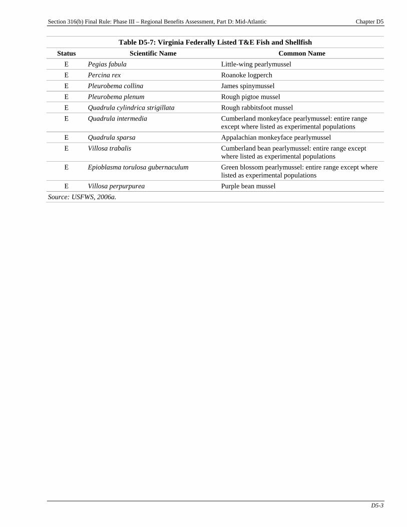
Section 316(b) Final Rule: Phase III – Regional Benefits Assessment, Part D: Mid-Atlantic Chapter D5
D5-3
Table D5-7: Virginia Federally Listed T&E Fish and Shellfish Status Scientific Name Common Name
E Pegias fabula Little-wing pearlymussel E Percina rex Roanoke logperch E Pleurobema collina James spinymussel E Pleurobema plenum Rough pigtoe mussel E Quadrula cylindrica strigillata Rough rabbitsfoot mussel E Quadrula intermedia Cumberland monkeyface pearlymussel: entire range
except where listed as experimental populations E Quadrula sparsa Appalachian monkeyface pearlymussel E Villosa trabalis Cumberland bean pearlymussel: entire range except
where listed as experimental populations E Epioblasma torulosa gubernaculum Green blossom pearlymussel: entire range except where
listed as experimental populations E Villosa perpurpurea Purple bean mussel
Source: USFWS, 2006a.

Section 316(b) Final Rule: Phase III – Regional Benefits Assessment
Part E: Gulf of Mexico

Section 316(b) Final Rule: Phase III – Regional Benefits Assessment, Part E: Gulf of Mexico Chapter E1
E1-1
Chapter E1: Background Introduction This chapter presents an overview of the potential Phase III existing facilities in the Gulf of Mexico study region and summarizes their key cooling water and compliance characteristics. For further discussion of the technical and compliance characteristics of potential Phase III existing facilities, refer to the Economic Analysis for the Final Section 316(b) Rule for Phase III Facilities and the Technical Development Document for the Final Section 316(b) Rule for Phase III Facilities (U.S. EPA, 2006a,c).
Chapter Contents E1-1 Facility Characteristics.................................. E1-1
E1-1 Facility Characteristics The Gulf of Mexico Regional Study includes five sample facilities that are potentially subject to the national standards for Phase III existing facilities. Figure E1-1 presents a map of these facilities. All five facilities are manufacturing facilities. Industry-wide, these five sample facilities represent 12 manufacturing facilities.PF
1FP
P
1P EPA applied sample weights to the survey respondents to account for non-sampled facilities and facilities that did
not respond to the survey. For more information on EPA’s 2000 Section 316(b) Industry Survey, please refer to the Information Collection Request (U.S. EPA, 2000b).
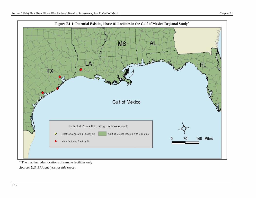
Section 316(b) Final Rule: Phase III – Regional Benefits Assessment, Part E: Gulf of Mexico Chapter E1
E1-2
Figure E1-1: Potential Existing Phase III Facilities in the Gulf of Mexico Regional StudyP
aP
P
aP The map includes locations of sample facilities only.
Source: U.S. EPA analysis for this report.
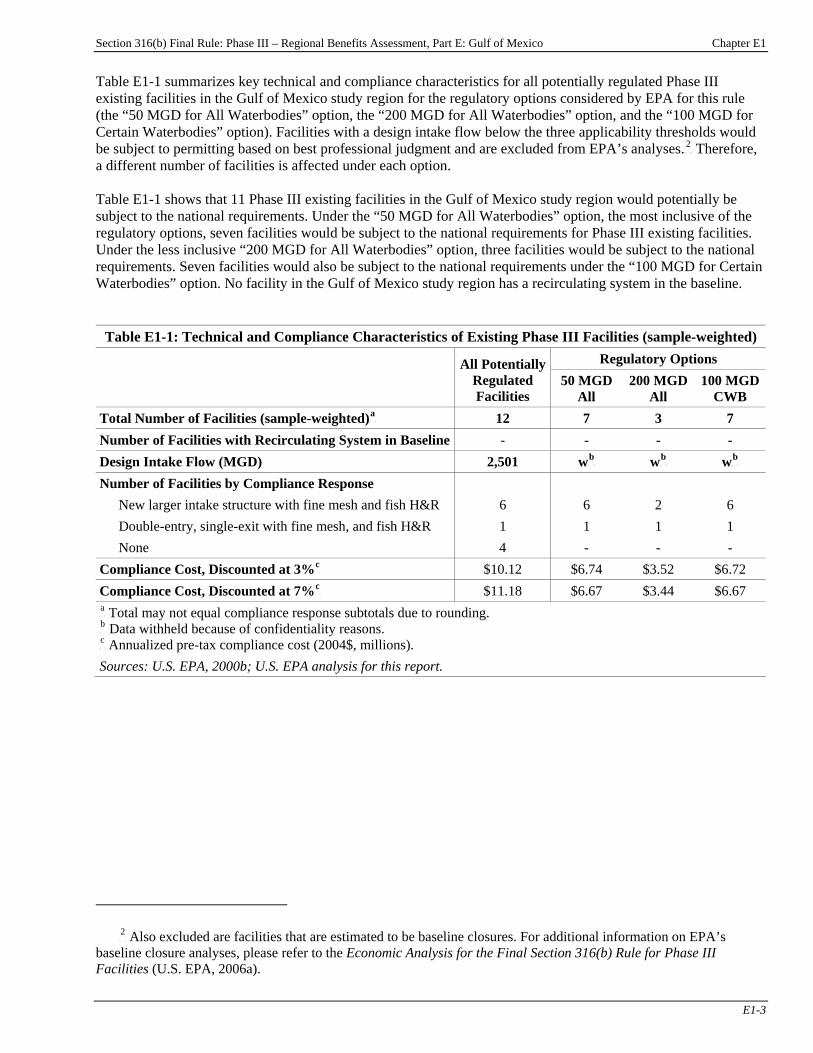
Section 316(b) Final Rule: Phase III – Regional Benefits Assessment, Part E: Gulf of Mexico Chapter E1
E1-3
Table E1-1 summarizes key technical and compliance characteristics for all potentially regulated Phase III existing facilities in the Gulf of Mexico study region for the regulatory options considered by EPA for this rule (the “50 MGD for All Waterbodies” option, the “200 MGD for All Waterbodies” option, and the “100 MGD for Certain Waterbodies” option). Facilities with a design intake flow below the three applicability thresholds would be subject to permitting based on best professional judgment and are excluded from EPA’s analyses.PF
2FP Therefore,
a different number of facilities is affected under each option. Table E1-1 shows that 11 Phase III existing facilities in the Gulf of Mexico study region would potentially be subject to the national requirements. Under the “50 MGD for All Waterbodies” option, the most inclusive of the regulatory options, seven facilities would be subject to the national requirements for Phase III existing facilities. Under the less inclusive “200 MGD for All Waterbodies” option, three facilities would be subject to the national requirements. Seven facilities would also be subject to the national requirements under the “100 MGD for Certain Waterbodies” option. No facility in the Gulf of Mexico study region has a recirculating system in the baseline.
Table E1-1: Technical and Compliance Characteristics of Existing Phase III Facilities (sample-weighted) Regulatory Options All Potentially
Regulated Facilities
50 MGD All
200 MGD All
100 MGD CWB
Total Number of Facilities (sample-weighted)P
aP 12 7 3 7
Number of Facilities with Recirculating System in Baseline - - - - Design Intake Flow (MGD) 2,501 wP
bP wP
bP wP
bP
Number of Facilities by Compliance Response New larger intake structure with fine mesh and fish H&R 6 6 2 6 Double-entry, single-exit with fine mesh, and fish H&R 1 1 1 1 None 4 - - -
Compliance Cost, Discounted at 3%P
cP $10.12 $6.74 $3.52 $6.72
Compliance Cost, Discounted at 7%P
cP $11.18 $6.67 $3.44 $6.67
P
aP Total may not equal compliance response subtotals due to rounding.
P
bP Data withheld because of confidentiality reasons.
P
cP Annualized pre-tax compliance cost (2004$, millions).
Sources: U.S. EPA, 2000b; U.S. EPA analysis for this report.
P
2P Also excluded are facilities that are estimated to be baseline closures. For additional information on EPA’s
baseline closure analyses, please refer to the Economic Analysis for the Final Section 316(b) Rule for Phase III Facilities (U.S. EPA, 2006a).
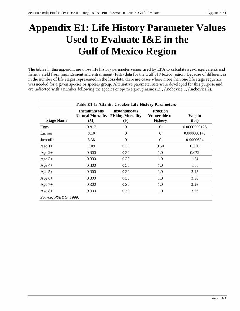
Section 316(b) Final Rule: Phase III – Regional Benefits Assessment, Part E: Gulf of Mexico Appendix E1
App. E1-1
Appendix E1: Life History Parameter Values Used to Evaluate I&E in the
Gulf of Mexico Region The tables in this appendix are those life history parameter values used by EPA to calculate age-1 equivalents and fishery yield from impingement and entrainment (I&E) data for the Gulf of Mexico region. Because of differences in the number of life stages represented in the loss data, there are cases where more than one life stage sequence was needed for a given species or species group. Alternative parameter sets were developed for this purpose and are indicated with a number following the species or species group name (i.e., Anchovies 1, Anchovies 2).
Table E1-1: Atlantic Croaker Life History Parameters
Stage Name
Instantaneous Natural Mortality
(M)
Instantaneous Fishing Mortality
(F)
Fraction Vulnerable to
Fishery Weight
(lbs) Eggs 0.817 0 0 0.0000000128 Larvae 8.10 0 0 0.000000145 Juvenile 3.38 0 0 0.0000624 Age 1+ 1.09 0.30 0.50 0.220 Age 2+ 0.300 0.30 1.0 0.672 Age 3+ 0.300 0.30 1.0 1.24 Age 4+ 0.300 0.30 1.0 1.88 Age 5+ 0.300 0.30 1.0 2.43 Age 6+ 0.300 0.30 1.0 3.26 Age 7+ 0.300 0.30 1.0 3.26 Age 8+ 0.300 0.30 1.0 3.26 Source: PSE&G, 1999.
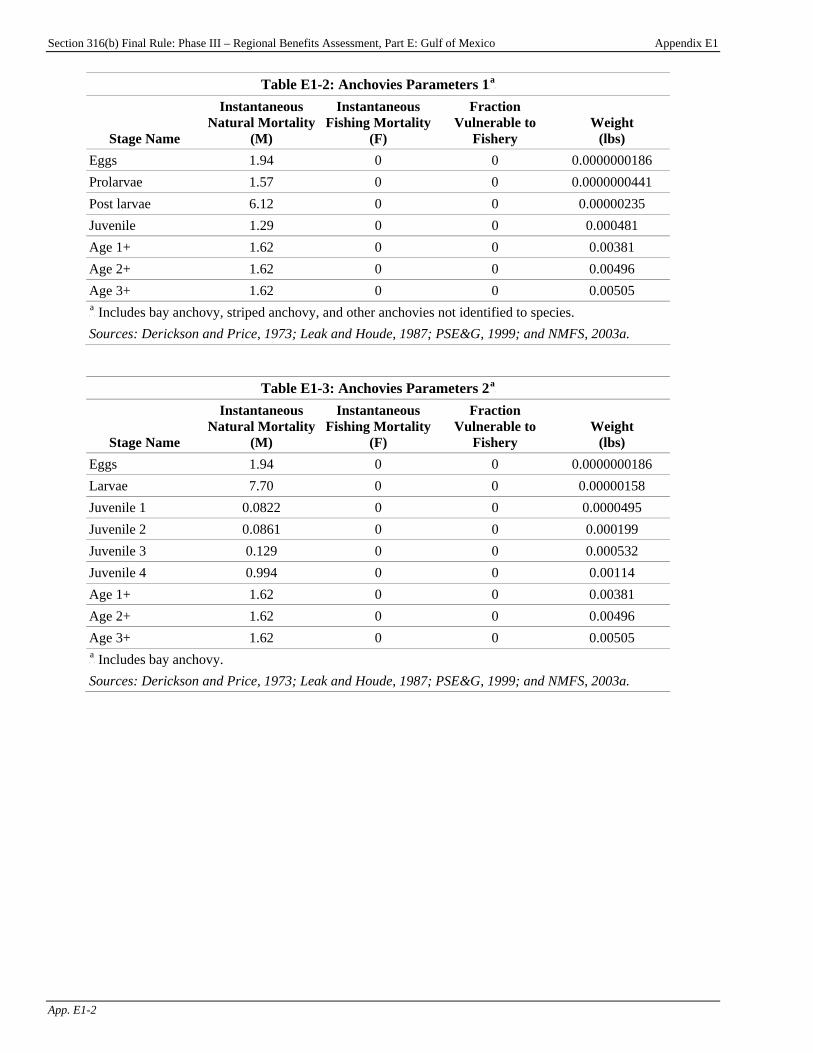
Section 316(b) Final Rule: Phase III – Regional Benefits Assessment, Part E: Gulf of Mexico Appendix E1
App. E1-2
Table E1-2: Anchovies Parameters 1P
aP
Stage Name
Instantaneous Natural Mortality
(M)
Instantaneous Fishing Mortality
(F)
Fraction Vulnerable to
Fishery Weight
(lbs) Eggs 1.94 0 0 0.0000000186 Prolarvae 1.57 0 0 0.0000000441 Post larvae 6.12 0 0 0.00000235 Juvenile 1.29 0 0 0.000481 Age 1+ 1.62 0 0 0.00381 Age 2+ 1.62 0 0 0.00496 Age 3+ 1.62 0 0 0.00505 P
aP Includes bay anchovy, striped anchovy, and other anchovies not identified to species.
Sources: Derickson and Price, 1973; Leak and Houde, 1987; PSE&G, 1999; and NMFS, 2003a.
Table E1-3: Anchovies Parameters 2P
aP
Stage Name
Instantaneous Natural Mortality
(M)
Instantaneous Fishing Mortality
(F)
Fraction Vulnerable to
Fishery Weight
(lbs) Eggs 1.94 0 0 0.0000000186 Larvae 7.70 0 0 0.00000158 Juvenile 1 0.0822 0 0 0.0000495 Juvenile 2 0.0861 0 0 0.000199 Juvenile 3 0.129 0 0 0.000532 Juvenile 4 0.994 0 0 0.00114 Age 1+ 1.62 0 0 0.00381 Age 2+ 1.62 0 0 0.00496 Age 3+ 1.62 0 0 0.00505 P
aP Includes bay anchovy.
Sources: Derickson and Price, 1973; Leak and Houde, 1987; PSE&G, 1999; and NMFS, 2003a.
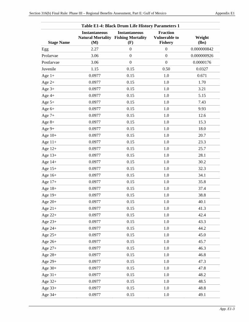
Section 316(b) Final Rule: Phase III – Regional Benefits Assessment, Part E: Gulf of Mexico Appendix E1
App. E1-3
Table E1-4: Black Drum Life History Parameters 1
Stage Name
Instantaneous Natural Mortality
(M)
Instantaneous Fishing Mortality
(F)
Fraction Vulnerable to
Fishery Weight
(lbs) Egg 2.27 0 0 0.000000842 Prolarvae 3.06 0 0 0.000000926 Postlarvae 3.06 0 0 0.0000176 Juvenile 1.15 0.15 0.50 0.0327 Age 1+ 0.0977 0.15 1.0 0.671 Age 2+ 0.0977 0.15 1.0 1.70 Age 3+ 0.0977 0.15 1.0 3.21 Age 4+ 0.0977 0.15 1.0 5.15 Age 5+ 0.0977 0.15 1.0 7.43 Age 6+ 0.0977 0.15 1.0 9.93 Age 7+ 0.0977 0.15 1.0 12.6 Age 8+ 0.0977 0.15 1.0 15.3 Age 9+ 0.0977 0.15 1.0 18.0 Age 10+ 0.0977 0.15 1.0 20.7 Age 11+ 0.0977 0.15 1.0 23.3 Age 12+ 0.0977 0.15 1.0 25.7 Age 13+ 0.0977 0.15 1.0 28.1 Age 14+ 0.0977 0.15 1.0 30.2 Age 15+ 0.0977 0.15 1.0 32.3 Age 16+ 0.0977 0.15 1.0 34.1 Age 17+ 0.0977 0.15 1.0 35.8 Age 18+ 0.0977 0.15 1.0 37.4 Age 19+ 0.0977 0.15 1.0 38.8 Age 20+ 0.0977 0.15 1.0 40.1 Age 21+ 0.0977 0.15 1.0 41.3 Age 22+ 0.0977 0.15 1.0 42.4 Age 23+ 0.0977 0.15 1.0 43.3 Age 24+ 0.0977 0.15 1.0 44.2 Age 25+ 0.0977 0.15 1.0 45.0 Age 26+ 0.0977 0.15 1.0 45.7 Age 27+ 0.0977 0.15 1.0 46.3 Age 28+ 0.0977 0.15 1.0 46.8 Age 29+ 0.0977 0.15 1.0 47.3 Age 30+ 0.0977 0.15 1.0 47.8 Age 31+ 0.0977 0.15 1.0 48.2 Age 32+ 0.0977 0.15 1.0 48.5 Age 33+ 0.0977 0.15 1.0 48.8 Age 34+ 0.0977 0.15 1.0 49.1

Section 316(b) Final Rule: Phase III – Regional Benefits Assessment, Part E: Gulf of Mexico Appendix E1
App. E1-4
Table E1-4: Black Drum Life History Parameters 1
Stage Name
Instantaneous Natural Mortality
(M)
Instantaneous Fishing Mortality
(F)
Fraction Vulnerable to
Fishery Weight
(lbs) Age 35+ 0.0977 0.15 1.0 49.4 Age 36+ 0.0977 0.15 1.0 49.6 Age 37+ 0.0977 0.15 1.0 49.8 Age 38+ 0.0977 0.15 1.0 50.0 Age 39+ 0.0977 0.15 1.0 50.1 Age 40+ 0.0977 0.15 1.0 50.3 Sources: Sutter et al., 1986; Scott and Scott, 1988; Murphy and Taylor, 1989; Leard et al., 1993; Bartell and Campbell, 2000; Froese and Pauly, 2001; and personal communication with Michael D. Murphy, Florida Fish and Wildlife Conservation Commission, Florida Marine Research Institute, January 23, 2002.
Table E1-5: Black Drum Life History Parameters 2
Stage Name
Instantaneous Natural Mortality
(M)
Instantaneous Fishing Mortality
(F)
Fraction Vulnerable to
Fishery Weight
(lbs) Egg 2.27 0 0 0.000000842 Larvae 6.13 0 0 0.00000453 Juvenile 1.15 0.15 0.50 0.0327 Age 1+ 0.0977 0.15 1.0 0.671 Age 2+ 0.0977 0.15 1.0 1.70 Age 3+ 0.0977 0.15 1.0 3.21 Age 4+ 0.0977 0.15 1.0 5.15 Age 5+ 0.0977 0.15 1.0 7.43 Age 6+ 0.0977 0.15 1.0 9.93 Age 7+ 0.0977 0.15 1.0 12.6 Age 8+ 0.0977 0.15 1.0 15.3 Age 9+ 0.0977 0.15 1.0 18.0 Age 10+ 0.0977 0.15 1.0 20.7 Age 11+ 0.0977 0.15 1.0 23.3 Age 12+ 0.0977 0.15 1.0 25.7 Age 13+ 0.0977 0.15 1.0 28.1 Age 14+ 0.0977 0.15 1.0 30.2 Age 15+ 0.0977 0.15 1.0 32.3 Age 16+ 0.0977 0.15 1.0 34.1 Age 17+ 0.0977 0.15 1.0 35.8 Age 18+ 0.0977 0.15 1.0 37.4 Age 19+ 0.0977 0.15 1.0 38.8 Age 20+ 0.0977 0.15 1.0 40.1

Section 316(b) Final Rule: Phase III – Regional Benefits Assessment, Part E: Gulf of Mexico Appendix E1
App. E1-5
Table E1-5: Black Drum Life History Parameters 2
Stage Name
Instantaneous Natural Mortality
(M)
Instantaneous Fishing Mortality
(F)
Fraction Vulnerable to
Fishery Weight
(lbs) Age 21+ 0.0977 0.15 1.0 41.3 Age 22+ 0.0977 0.15 1.0 42.4 Age 23+ 0.0977 0.15 1.0 43.3 Age 24+ 0.0977 0.15 1.0 44.2 Age 25+ 0.0977 0.15 1.0 45.0 Age 26+ 0.0977 0.15 1.0 45.7 Age 27+ 0.0977 0.15 1.0 46.3 Age 28+ 0.0977 0.15 1.0 46.8 Age 29+ 0.0977 0.15 1.0 47.3 Age 30+ 0.0977 0.15 1.0 47.8 Age 31+ 0.0977 0.15 1.0 48.2 Age 32+ 0.0977 0.15 1.0 48.5 Age 33+ 0.0977 0.15 1.0 48.8 Age 34+ 0.0977 0.15 1.0 49.1 Age 35+ 0.0977 0.15 1.0 49.4 Age 36+ 0.0977 0.15 1.0 49.6 Age 37+ 0.0977 0.15 1.0 49.8 Age 38+ 0.0977 0.15 1.0 50.0 Age 39+ 0.0977 0.15 1.0 50.1 Age 40+ 0.0977 0.15 1.0 50.3 Sources: Sutter et al., 1986; Scott and Scott, 1988; Murphy and Taylor, 1989; Leard et al., 1993; Able and Fahay, 1998; Bartell and Campbell, 2000; Froese and Pauly, 2001; and personal communication with Michael D. Murphy, Florida Fish and Wildlife Conservation Commission, Florida Marine Research Institute, January 23, 2002.
Table E1-6: Blue Crab Life History Parameters
Stage Name
Instantaneous Natural Mortality
(M)
Instantaneous Fishing Mortality
(F)
Fraction Vulnerable to
Fishery Weight
(lbs) Zoeae 13.8 0 0 0.000000211 Megalops 1.30 0 0 0.00000291 Juvenile 1.73 0.48 0.50 0.00000293 Age 1+ 1.00 1.0 1.0 0.00719 Age 2+ 1.00 1.0 1.0 0.113 Age 3+ 1.00 1.0 1.0 0.326 TSources: Hartman, 1993; PSE&G, 1999; and Murphy et al., 2000T.
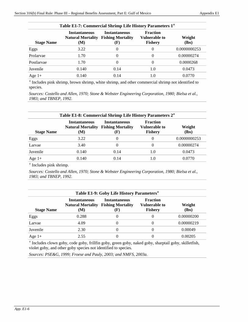
Section 316(b) Final Rule: Phase III – Regional Benefits Assessment, Part E: Gulf of Mexico Appendix E1
App. E1-6
Table E1-7: Commercial Shrimp Life History Parameters 1P
aP
Stage Name
Instantaneous Natural Mortality
(M)
Instantaneous Fishing Mortality
(F)
Fraction Vulnerable to
Fishery Weight
(lbs) Eggs 3.22 0 0 0.0000000253 Prolarvae 1.70 0 0 0.00000274 Postlarvae 1.70 0 0 0.0000268 Juvenile 0.140 0.14 1.0 0.0473 Age 1+ 0.140 0.14 1.0 0.0770 P
aP Includes pink shrimp, brown shrimp, white shrimp, and other commercial shrimp not identified to
species. Sources: Costello and Allen, 1970; Stone & Webster Engineering Corporation, 1980; Bielsa et al., 1983; and TBNEP, 1992.
Table E1-8: Commercial Shrimp Life History Parameters 2P
aP
Stage Name
Instantaneous Natural Mortality
(M)
Instantaneous Fishing Mortality
(F)
Fraction Vulnerable to
Fishery Weight
(lbs) Eggs 3.22 0 0 0.0000000253 Larvae 3.40 0 0 0.00000274 Juvenile 0.140 0.14 1.0 0.0473 Age 1+ 0.140 0.14 1.0 0.0770 P
aP Includes pink shrimp.
Sources: Costello and Allen, 1970; Stone & Webster Engineering Corporation, 1980; Bielsa et al., 1983; and TBNEP, 1992.
Table E1-9: Goby Life History ParametersP
aP
Stage Name
Instantaneous Natural Mortality
(M)
Instantaneous Fishing Mortality
(F)
Fraction Vulnerable to
Fishery Weight
(lbs) Eggs 0.288 0 0 0.00000200 Larvae 4.09 0 0 0.00000219 Juvenile 2.30 0 0 0.00049 Age 1+ 2.55 0 0 0.00205 P
aP Includes clown goby, code goby, frillfin goby, green goby, naked goby, sharptail goby, skilletfish,
violet goby, and other goby species not identified to species. Sources: PSE&G, 1999; Froese and Pauly, 2003; and NMFS, 2003a.
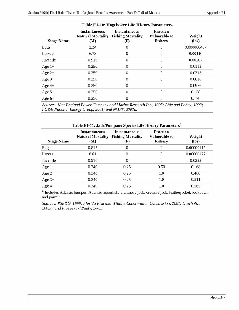
Section 316(b) Final Rule: Phase III – Regional Benefits Assessment, Part E: Gulf of Mexico Appendix E1
App. E1-7
Table E1-10: Hogchoker Life History Parameters
Stage Name
Instantaneous Natural Mortality
(M)
Instantaneous Fishing Mortality
(F)
Fraction Vulnerable to
Fishery Weight
(lbs) Eggs 2.24 0 0 0.000000487 Larvae 6.73 0 0 0.00110 Juvenile 0.916 0 0 0.00207 Age 1+ 0.250 0 0 0.0113 Age 2+ 0.250 0 0 0.0313 Age 3+ 0.250 0 0 0.0610 Age 4+ 0.250 0 0 0.0976 Age 5+ 0.250 0 0 0.138 Age 6+ 0.250 0 0 0.178 TSources: New England Power Company and Marine Research Inc., 1995;T Able and Fahay, 1998; PG&E National Energy Group, 2001; and NMFS, 2003a.
Table E1-11: Jack/Pompano Species Life History ParametersP
aP
Stage Name
Instantaneous Natural Mortality
(M)
Instantaneous Fishing Mortality
(F)
Fraction Vulnerable to
Fishery Weight
(lbs) Eggs 0.817 0 0 0.00000115 Larvae 8.61 0 0 0.00000127 Juvenile 0.916 0 0 0.0222 Age 1+ 0.340 0.25 0.50 0.168 Age 2+ 0.340 0.25 1.0 0.460 Age 3+ 0.340 0.25 1.0 0.511 Age 4+ 0.340 0.25 1.0 0.565 P
aP Includes Atlantic bumper, Atlantic moonfish, bluntnose jack, crevalle jack, leatherjacket, lookdown,
and permit. Sources: PSE&G, 1999; Florida Fish and Wildlife Conservation Commission, 2001; Overholtz, 2002b; and Froese and Pauly, 2003.
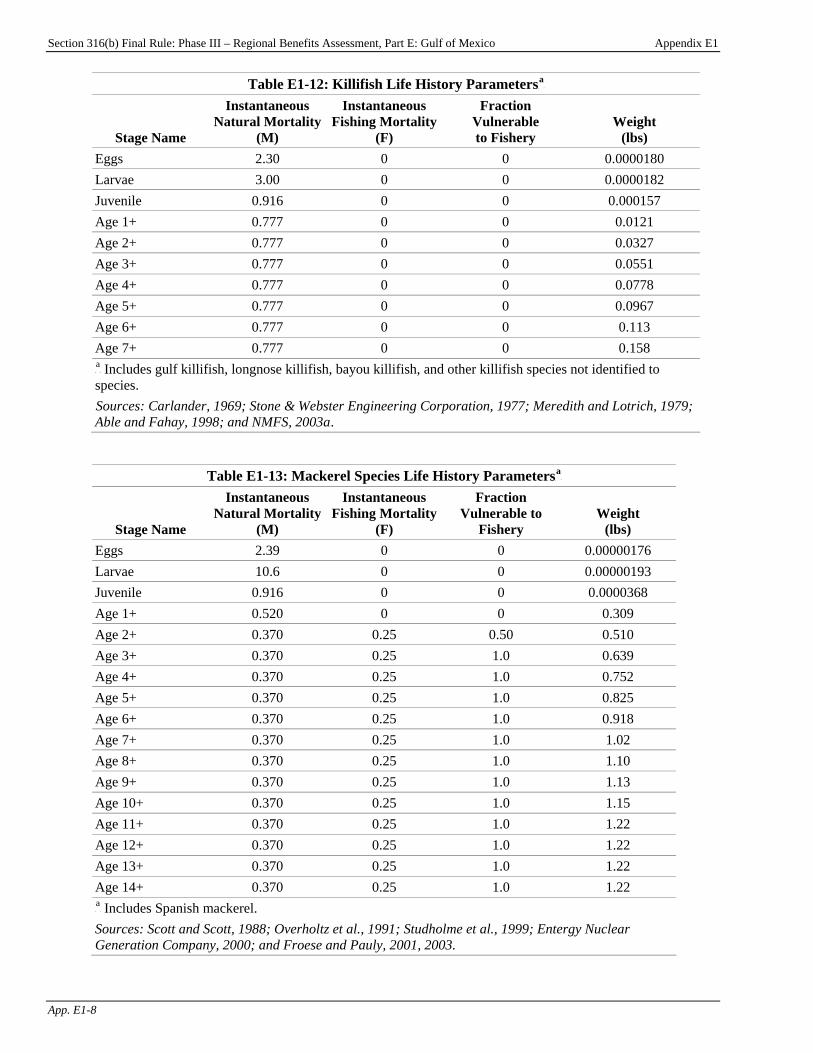
Section 316(b) Final Rule: Phase III – Regional Benefits Assessment, Part E: Gulf of Mexico Appendix E1
App. E1-8
Table E1-12: Killifish Life History ParametersP
aP
Stage Name
Instantaneous Natural Mortality
(M)
Instantaneous Fishing Mortality
(F)
Fraction Vulnerable to Fishery
Weight (lbs)
Eggs 2.30 0 0 0.0000180 Larvae 3.00 0 0 0.0000182 Juvenile 0.916 0 0 0.000157 Age 1+ 0.777 0 0 0.0121 Age 2+ 0.777 0 0 0.0327 Age 3+ 0.777 0 0 0.0551 Age 4+ 0.777 0 0 0.0778 Age 5+ 0.777 0 0 0.0967 Age 6+ 0.777 0 0 0.113 Age 7+ 0.777 0 0 0.158 P
aP Includes gulf killifish, longnose killifish, bayou killifish, and other killifish species not identified to
species. TSources: Carlander, 1969; Stone & Webster Engineering Corporation, 1977; Meredith and Lotrich, 1979; Able and Fahay, 1998; and NMFS, 2003aT.
Table E1-13: Mackerel Species Life History ParametersP
aP
Stage Name
Instantaneous Natural Mortality
(M)
Instantaneous Fishing Mortality
(F)
Fraction Vulnerable to
Fishery Weight
(lbs) Eggs 2.39 0 0 0.00000176 Larvae 10.6 0 0 0.00000193 Juvenile 0.916 0 0 0.0000368 Age 1+ 0.520 0 0 0.309 Age 2+ 0.370 0.25 0.50 0.510 Age 3+ 0.370 0.25 1.0 0.639 Age 4+ 0.370 0.25 1.0 0.752 Age 5+ 0.370 0.25 1.0 0.825 Age 6+ 0.370 0.25 1.0 0.918 Age 7+ 0.370 0.25 1.0 1.02 Age 8+ 0.370 0.25 1.0 1.10 Age 9+ 0.370 0.25 1.0 1.13 Age 10+ 0.370 0.25 1.0 1.15 Age 11+ 0.370 0.25 1.0 1.22 Age 12+ 0.370 0.25 1.0 1.22 Age 13+ 0.370 0.25 1.0 1.22 Age 14+ 0.370 0.25 1.0 1.22 P
aP Includes Spanish mackerel.
Sources: Scott and Scott, 1988; Overholtz et al., 1991; Studholme et al., 1999; Entergy Nuclear Generation Company, 2000; and Froese and Pauly, 2001, 2003.
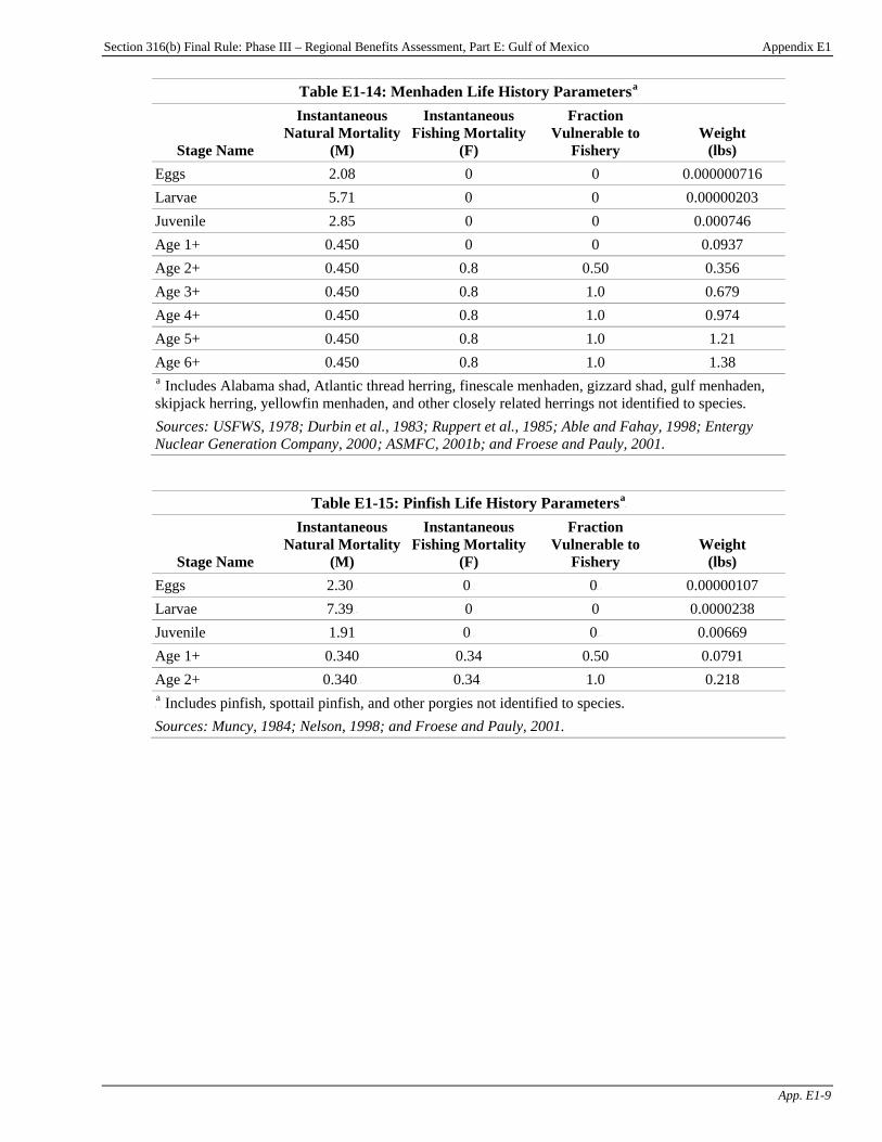
Section 316(b) Final Rule: Phase III – Regional Benefits Assessment, Part E: Gulf of Mexico Appendix E1
App. E1-9
Table E1-14: Menhaden Life History ParametersP
aP
Stage Name
Instantaneous Natural Mortality
(M)
Instantaneous Fishing Mortality
(F)
Fraction Vulnerable to
Fishery Weight
(lbs) Eggs 2.08 0 0 0.000000716 Larvae 5.71 0 0 0.00000203 Juvenile 2.85 0 0 0.000746 Age 1+ 0.450 0 0 0.0937 Age 2+ 0.450 0.8 0.50 0.356 Age 3+ 0.450 0.8 1.0 0.679 Age 4+ 0.450 0.8 1.0 0.974 Age 5+ 0.450 0.8 1.0 1.21 Age 6+ 0.450 0.8 1.0 1.38 P
aP Includes Alabama shad, Atlantic thread herring, finescale menhaden, gizzard shad, gulf menhaden,
skipjack herring, yellowfin menhaden, and other closely related herrings not identified to species. TSources: USFWS, 1978; Durbin et al., 1983; Ruppert et al., 1985; Able and Fahay, 1998; Entergy Nuclear Generation Company, 2000T; ASMFC, 2001b; and Froese and Pauly, 2001.
Table E1-15: Pinfish Life History ParametersP
aP
Stage Name
Instantaneous Natural Mortality
(M)
Instantaneous Fishing Mortality
(F)
Fraction Vulnerable to
Fishery Weight
(lbs) Eggs 2.30P
P 0P
P 0P
P 0.00000107
Larvae 7.39P
P 0 0 0.0000238
Juvenile 1.91 0P
P 0P
P 0.00669
Age 1+ 0.340 0.34 0.50 0.0791 Age 2+ 0.340P
P 0.34P
P 1.0 0.218
P
aP Includes pinfish, spottail pinfish, and other porgies not identified to species.
Sources: Muncy, 1984; Nelson, 1998; and Froese and Pauly, 2001.
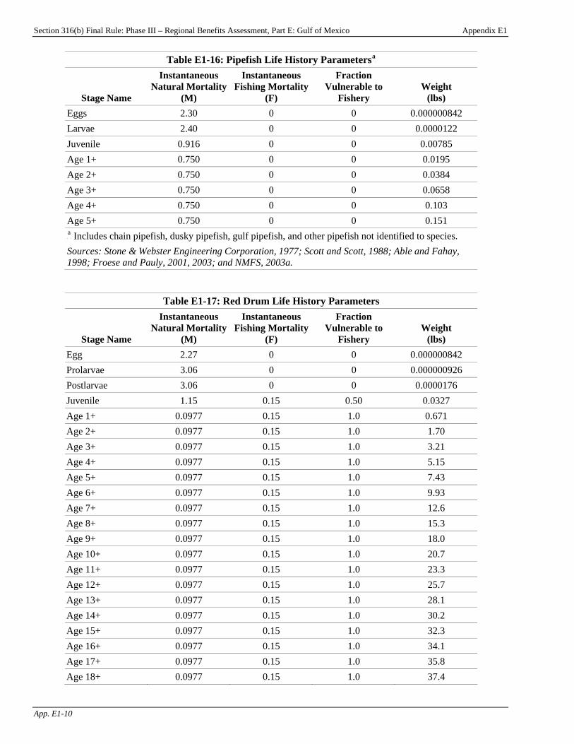
Section 316(b) Final Rule: Phase III – Regional Benefits Assessment, Part E: Gulf of Mexico Appendix E1
App. E1-10
Table E1-16: Pipefish Life History ParametersP
aP
Stage Name
Instantaneous Natural Mortality
(M)
Instantaneous Fishing Mortality
(F)
Fraction Vulnerable to
Fishery Weight
(lbs) Eggs 2.30 0 0 0.000000842 Larvae 2.40 0 0 0.0000122 Juvenile 0.916 0 0 0.00785 Age 1+ 0.750 0 0 0.0195 Age 2+ 0.750 0 0 0.0384 Age 3+ 0.750 0 0 0.0658 Age 4+ 0.750 0 0 0.103 Age 5+ 0.750 0 0 0.151 P
aP Includes chain pipefish, dusky pipefish, gulf pipefish, and other pipefish not identified to species.
Sources: Stone & Webster Engineering Corporation, 1977; Scott and Scott, 1988; Able and Fahay, 1998; Froese and Pauly, 2001, 2003; and NMFS, 2003a.
Table E1-17: Red Drum Life History Parameters
Stage Name
Instantaneous Natural Mortality
(M)
Instantaneous Fishing Mortality
(F)
Fraction Vulnerable to
Fishery Weight
(lbs) Egg 2.27 0 0 0.000000842 Prolarvae 3.06 0 0 0.000000926 Postlarvae 3.06 0 0 0.0000176 Juvenile 1.15 0.15 0.50 0.0327 Age 1+ 0.0977 0.15 1.0 0.671 Age 2+ 0.0977 0.15 1.0 1.70 Age 3+ 0.0977 0.15 1.0 3.21 Age 4+ 0.0977 0.15 1.0 5.15 Age 5+ 0.0977 0.15 1.0 7.43 Age 6+ 0.0977 0.15 1.0 9.93 Age 7+ 0.0977 0.15 1.0 12.6 Age 8+ 0.0977 0.15 1.0 15.3 Age 9+ 0.0977 0.15 1.0 18.0 Age 10+ 0.0977 0.15 1.0 20.7 Age 11+ 0.0977 0.15 1.0 23.3 Age 12+ 0.0977 0.15 1.0 25.7 Age 13+ 0.0977 0.15 1.0 28.1 Age 14+ 0.0977 0.15 1.0 30.2 Age 15+ 0.0977 0.15 1.0 32.3 Age 16+ 0.0977 0.15 1.0 34.1 Age 17+ 0.0977 0.15 1.0 35.8 Age 18+ 0.0977 0.15 1.0 37.4

Section 316(b) Final Rule: Phase III – Regional Benefits Assessment, Part E: Gulf of Mexico Appendix E1
App. E1-11
Table E1-17: Red Drum Life History Parameters
Stage Name
Instantaneous Natural Mortality
(M)
Instantaneous Fishing Mortality
(F)
Fraction Vulnerable to
Fishery Weight
(lbs) Age 19+ 0.0977 0.15 1.0 38.8 Age 20+ 0.0977 0.15 1.0 40.1 Age 21+ 0.0977 0.15 1.0 41.3 Age 22+ 0.0977 0.15 1.0 42.4 Age 23+ 0.0977 0.15 1.0 43.3 Age 24+ 0.0977 0.15 1.0 44.2 Age 25+ 0.0977 0.15 1.0 45.0 Age 26+ 0.0977 0.15 1.0 45.7 Age 27+ 0.0977 0.15 1.0 46.3 Age 28+ 0.0977 0.15 1.0 46.8 Age 29+ 0.0977 0.15 1.0 47.3 Age 30+ 0.0977 0.15 1.0 47.8 Age 31+ 0.0977 0.15 1.0 48.2 Age 32+ 0.0977 0.15 1.0 48.5 Age 33+ 0.0977 0.15 1.0 48.8 Age 34+ 0.0977 0.15 1.0 49.1 Age 35+ 0.0977 0.15 1.0 49.4 Age 36+ 0.0977 0.15 1.0 49.6 Age 37+ 0.0977 0.15 1.0 49.8 Age 38+ 0.0977 0.15 1.0 50.0 Age 39+ 0.0977 0.15 1.0 50.1 Age 40+ 0.0977 0.15 1.0 50.3 Sources: Sutter et al., 1986; Scott and Scott, 1988; Murphy and Taylor, 1989; Leard et al., 1993; Bartell and Campbell, 2000; Froese and Pauly, 2001; and personal communication with Michael D. Murphy, Florida Fish and Wildlife Conservation Commission, Florida Marine Research Institute, January 23, 2002.
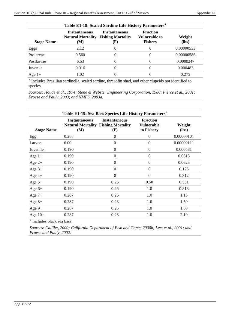
Section 316(b) Final Rule: Phase III – Regional Benefits Assessment, Part E: Gulf of Mexico Appendix E1
App. E1-12
Table E1-18: Scaled Sardine Life History ParametersP
aP
Stage Name
Instantaneous Natural Mortality
(M)
Instantaneous Fishing Mortality
(F)
Fraction Vulnerable to
Fishery Weight
(lbs) Eggs 2.12 0 0 0.00000533 Prolarvae 0.560 0 0 0.00000586 Postlarvae 6.53 0 0 0.0000247 Juvenile 0.916 0 0 0.000483 Age 1+ 1.02 0 0 0.275 P
aP Includes Brazilian sardinella, scaled sardine, threadfin shad, and other clupeids not identified to
species. Sources: Houde et al., 1974; Stone & Webster Engineering Corporation, 1980; Pierce et al., 2001; Froese and Pauly, 2003; and NMFS, 2003a.
Table E1-19: Sea Bass Species Life History ParametersP
aP
Stage Name
Instantaneous Natural Mortality
(M)
Instantaneous Fishing Mortality
(F)
Fraction Vulnerable to Fishery
Weight (lbs)
Egg 0.288 0 0 0.00000101 Larvae 6.00 0 0 0.00000111 Juvenile 0.190 0 0 0.000581 Age 1+ 0.190 0 0 0.0313 Age 2+ 0.190 0 0 0.0625 Age 3+ 0.190 0 0 0.125 Age 4+ 0.190 0 0 0.312 Age 5+ 0.190 0.26 0.50 0.531 Age 6+ 0.190 0.26 1.0 0.813 Age 7+ 0.287 0.26 1.0 1.13 Age 8+ 0.287 0.26 1.0 1.50 Age 9+ 0.287 0.26 1.0 1.88 Age 10+ 0.287 0.26 1.0 2.19 P
aP Includes black sea bass.
Sources: Cailliet, 2000; California Department of Fish and Game, 2000b; Leet et al., 2001; and Froese and Pauly, 2002.
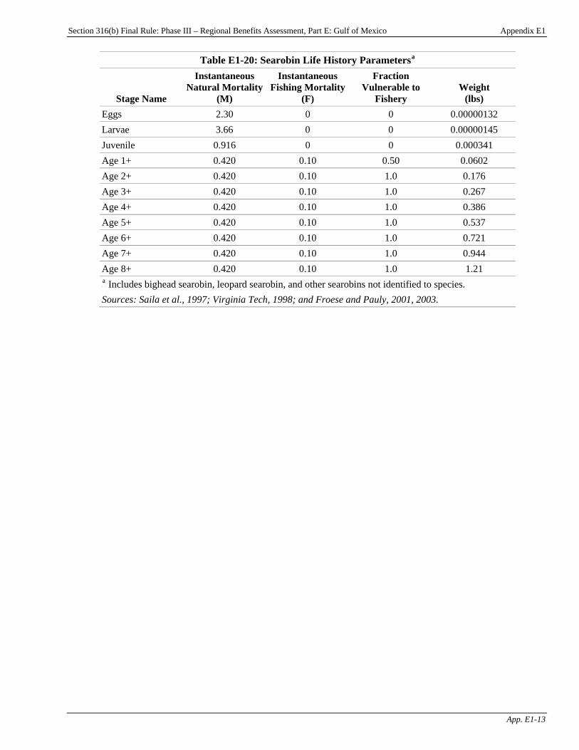
Section 316(b) Final Rule: Phase III – Regional Benefits Assessment, Part E: Gulf of Mexico Appendix E1
App. E1-13
Table E1-20: Searobin Life History ParametersP
aP
Stage Name
Instantaneous Natural Mortality
(M)
Instantaneous Fishing Mortality
(F)
Fraction Vulnerable to
Fishery Weight
(lbs) Eggs 2.30 0 0 0.00000132 Larvae 3.66 0 0 0.00000145 Juvenile 0.916 0 0 0.000341 Age 1+ 0.420 0.10 0.50 0.0602 Age 2+ 0.420 0.10 1.0 0.176 Age 3+ 0.420 0.10 1.0 0.267 Age 4+ 0.420 0.10 1.0 0.386 Age 5+ 0.420 0.10 1.0 0.537 Age 6+ 0.420 0.10 1.0 0.721 Age 7+ 0.420 0.10 1.0 0.944 Age 8+ 0.420 0.10 1.0 1.21 P
aP Includes bighead searobin, leopard searobin, and other searobins not identified to species.
Sources: Saila et al., 1997; Virginia Tech, 1998; and Froese and Pauly, 2001, 2003.
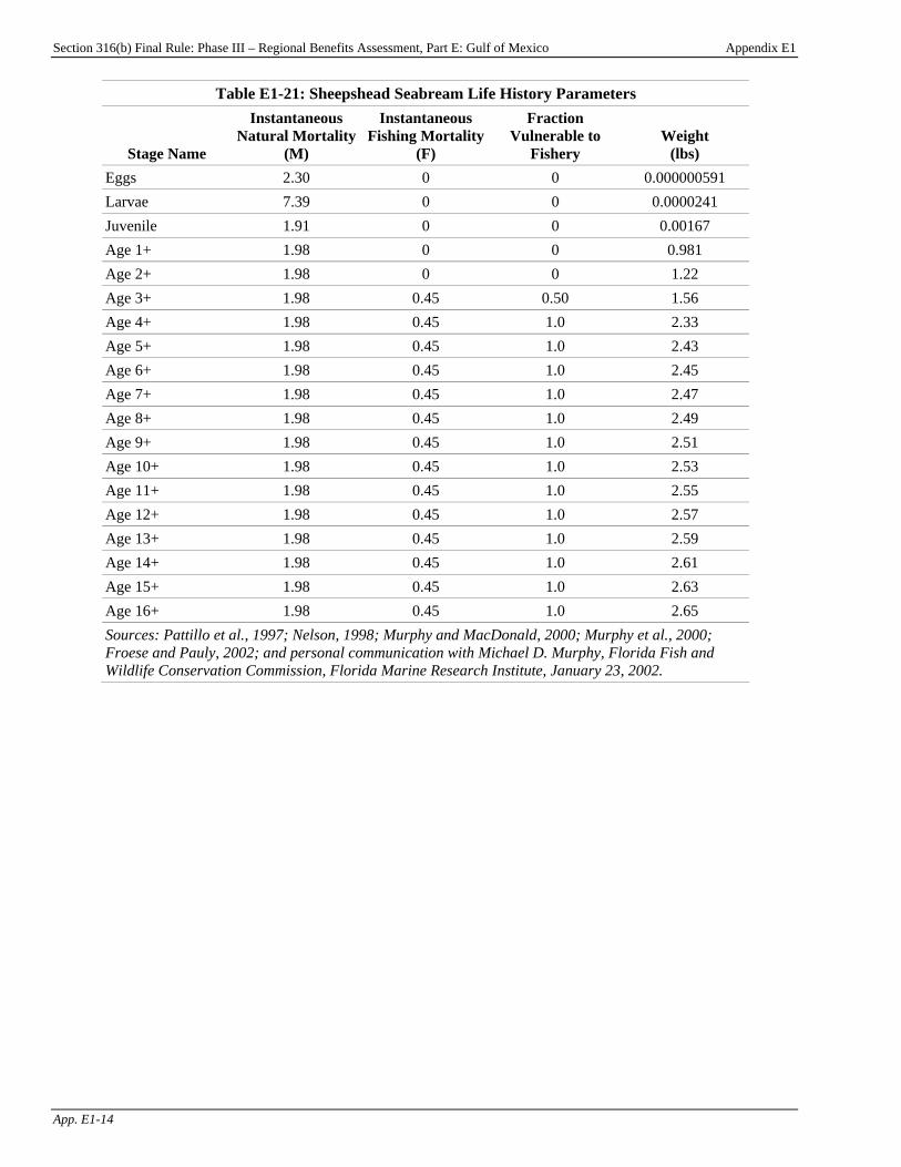
Section 316(b) Final Rule: Phase III – Regional Benefits Assessment, Part E: Gulf of Mexico Appendix E1
App. E1-14
Table E1-21: Sheepshead Seabream Life History Parameters
Stage Name
Instantaneous Natural Mortality
(M)
Instantaneous Fishing Mortality
(F)
Fraction Vulnerable to
Fishery Weight
(lbs) Eggs 2.30 0 0 0.000000591 Larvae 7.39 0 0 0.0000241 Juvenile 1.91 0 0 0.00167 Age 1+ 1.98 0 0 0.981 Age 2+ 1.98 0 0 1.22 Age 3+ 1.98 0.45 0.50 1.56 Age 4+ 1.98 0.45 1.0 2.33 Age 5+ 1.98 0.45 1.0 2.43 Age 6+ 1.98 0.45 1.0 2.45 Age 7+ 1.98 0.45 1.0 2.47 Age 8+ 1.98 0.45 1.0 2.49 Age 9+ 1.98 0.45 1.0 2.51 Age 10+ 1.98 0.45 1.0 2.53 Age 11+ 1.98 0.45 1.0 2.55 Age 12+ 1.98 0.45 1.0 2.57 Age 13+ 1.98 0.45 1.0 2.59 Age 14+ 1.98 0.45 1.0 2.61 Age 15+ 1.98 0.45 1.0 2.63 Age 16+ 1.98 0.45 1.0 2.65 Sources: Pattillo et al., 1997; Nelson, 1998; Murphy and MacDonald, 2000; Murphy et al., 2000; Froese and Pauly, 2002; and personal communication with Michael D. Murphy, Florida Fish and Wildlife Conservation Commission, Florida Marine Research Institute, January 23, 2002.

Section 316(b) Final Rule: Phase III – Regional Benefits Assessment, Part E: Gulf of Mexico Appendix E1
App. E1-15
Table E1-22: Silver Perch Life History Parameters 1P
aP
Stage Name
Instantaneous Natural Mortality
(M)
Instantaneous Fishing Mortality
(F)
Fraction Vulnerable to
Fishery Weight
(lbs) Eggs 2.75 0 0 0.000000527 Prolarvae 2.10 0 0 0.000000580 Postlarvae 3.27 0 0 0.0000379 Juvenile 1.71 0 0 0.0445 Age 1+ 3.84 0 0 0.273 Age 2+ 3.84 0.10 0.50 4.15 Age 3+ 3.84 0.10 1.0 0.607 P
aP Includes banded drum, silver perch, silver seatrout, southern kingfish, and star drum.
Sources: Able and Fahay, 1998; PSE&G, 1999; Florida Fish and Wildlife Conservation Commission, 2001; Froese and Pauly, 2001, 2003; and personal communication with Michael D. Murphy, Florida Fish and Wildlife Conservation Commission, Florida Marine Research Institute, January 23, 2002.
Table E1-23: Silver Perch Life History Parameters 2P
aP
Stage Name
Instantaneous Natural Mortality
(M)
Instantaneous Fishing Mortality
(F)
Fraction Vulnerable to
Fishery Weight
(lbs) Eggs 2.75 0 0 0.000000527 Larvae 5.37 0 0 0.00000771 Juvenile 1.71 0 0 0.0445 Age 1+ 3.84 0 0 0.273 Age 2+ 3.84 0.10 0.50 0.415 Age 3+ 3.84 0.10 1.0 0.607 P
aP Includes silver perch, northern kingfish, and southern kingfish.
Sources: Able and Fahay, 1998; PSE&G, 1999; Florida Fish and Wildlife Conservation Commission, 2001; Froese and Pauly, 2001, 2003; and personal communication with Michael D. Murphy, Florida Fish and Wildlife Conservation Commission, Florida Marine Research Institute, January 23, 2002.
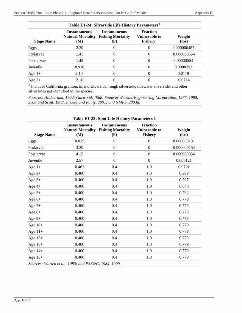
Section 316(b) Final Rule: Phase III – Regional Benefits Assessment, Part E: Gulf of Mexico Appendix E1
App. E1-16
Table E1-24: Silverside Life History ParametersP
aP
Stage Name
Instantaneous Natural Mortality
(M)
Instantaneous Fishing Mortality
(F)
Fraction Vulnerable to
FisheryP
P
Weight (lbs)
Eggs 2.30 0 0 0.000000487P
P
Prolarvae 1.45 0 0 0.000000554 Postlarvae 1.45 0 0 0.00000554P
P
Juvenile 0.916 0 0 0.0000292P
P
Age 1+ 2.10P
P 0 0 0.0119P
P
Age 2+ 2.10 0 0 0.0224 P
aP Includes California grunion, inland silverside, rough silverside, tidewater silverside, and other
silversides not identified to the species. TSources: Hildebrand, 1922; Garwood, 1968; Stone & Webster Engineering Corporation, 1977, 1980; Scott and Scott, 1988; Froese and Pauly, 2001; and NMFS, 2003aT.
Table E1-25: Spot Life History Parameters 1
Stage Name
Instantaneous Natural Mortality
(M)
Instantaneous Fishing Mortality
(F)
Fraction Vulnerable to
Fishery Weight
(lbs) Eggs 0.825 0 0 0.000000131 Prolarvae 3.30 0 0 0.000000154 Postlarvae 4.12 0 0 0.000000854 Juvenile 2.57 0 0 0.000121 Age 1+ 0.463 0.4 1.0 0.0791 Age 2+ 0.400 0.4 1.0 0.299 Age 3+ 0.400 0.4 1.0 0.507 Age 4+ 0.400 0.4 1.0 0.648 Age 5+ 0.400 0.4 1.0 0.732 Age 6+ 0.400 0.4 1.0 0.779 Age 7+ 0.400 0.4 1.0 0.779 Age 8+ 0.400 0.4 1.0 0.779 Age 9+ 0.400 0.4 1.0 0.779 Age 10+ 0.400 0.4 1.0 0.779 Age 11+ 0.400 0.4 1.0 0.779 Age 12+ 0.400 0.4 1.0 0.779 Age 13+ 0.400 0.4 1.0 0.779 Age 14+ 0.400 0.4 1.0 0.779 Age 15+ 0.400 0.4 1.0 0.779 Sources: Warlen et al., 1980; and PSE&G, 1984, 1999.

Section 316(b) Final Rule: Phase III – Regional Benefits Assessment, Part E: Gulf of Mexico Appendix E1
App. E1-17
Table E1-26: Spot Life History Parameters 2
Stage Name
Instantaneous Natural Mortality
(M)
Instantaneous Fishing Mortality
(F)
Fraction Vulnerable to
Fishery Weight
(lbs) Eggs 0.825P
P 0 0 0.000000131P
P
Larvae 7.42P
P 0 0 0.000000504
Juvenile 2.57 0 0 0.000121P
P
Age 1+ 0.463 0.4 1.0 0.0791P
P
Age 2+ 0.400P
P 0.4 1.0 0.299P
P
Age 3+ 0.400 0.4 1.0 0.507 Age 4+ 0.400P
P 0.4 1.0 0.648P
P
Age 5+ 0.400 0.4 1.0 0.732 Age 6+ 0.400P
P 0.4 1.0 0.779P
P
Age 7+ 0.400 0.4 1.0 0.779P
P
Age 8+ 0.400P
P 0.4 1.0 0.779
Age 9+ 0.400 0.4 1.0 0.779P
P
Age 10+ 0.400P
P 0.4 1.0 0.779
Age 11+ 0.400 0.4 1.0 0.779P
P
Age 12+ 0.400P
P 0.4 1.0 0.779
Age 13+ 0.400 0.4 1.0 0.779P
P
Age 14+ 0.400 0.4 1.0 0.779 Age 15+ 0.400P
P 0.4 1.0 0.779P
P
Sources: Warlen et al., 1980; and PSE&G, 1984, 1999.
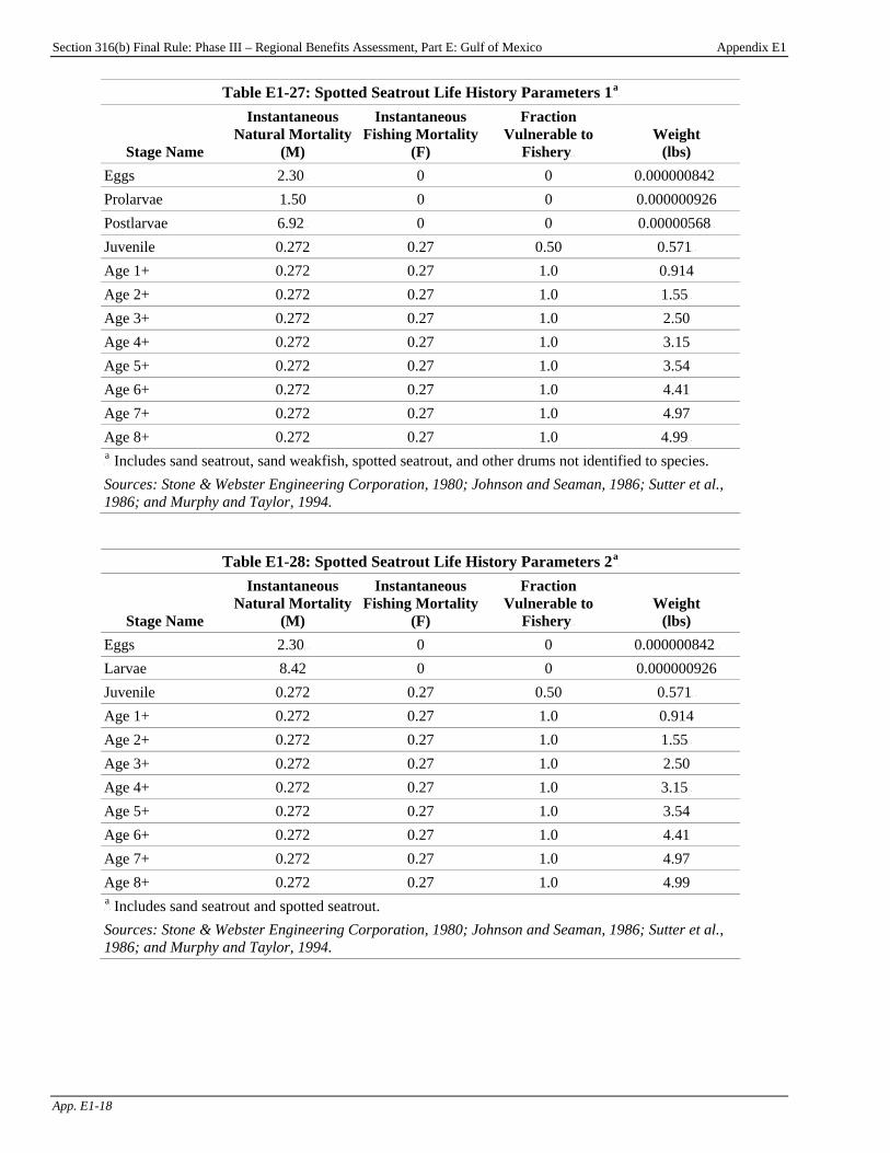
Section 316(b) Final Rule: Phase III – Regional Benefits Assessment, Part E: Gulf of Mexico Appendix E1
App. E1-18
Table E1-27: Spotted Seatrout Life History Parameters 1P
aP
Stage Name
Instantaneous Natural Mortality
(M)
Instantaneous Fishing Mortality
(F)
Fraction Vulnerable to
FisheryP
P
Weight (lbs)
Eggs 2.30P
P 0 0 0.000000842P
P
Prolarvae 1.50 0 0 0.000000926 Postlarvae 6.92P
P 0 0 0.00000568P
P
Juvenile 0.272 0.27 0.50 0.571P
P
Age 1+ 0.272 0.27 1.0 0.914 Age 2+ 0.272 0.27 1.0 1.55P
P
Age 3+ 0.272 0.27 1.0 2.50 Age 4+ 0.272 0.27 1.0 3.15 Age 5+ 0.272 0.27 1.0 3.54 Age 6+ 0.272 0.27 1.0 4.41 Age 7+ 0.272 0.27 1.0 4.97 Age 8+ 0.272 0.27 1.0 4.99P
P
P
aP Includes sand seatrout, sand weakfish, spotted seatrout, and other drums not identified to species.
Sources: Stone & Webster Engineering Corporation, 1980; Johnson and Seaman, 1986; Sutter et al., 1986; and Murphy and Taylor, 1994.
Table E1-28: Spotted Seatrout Life History Parameters 2P
aP
Stage Name
Instantaneous Natural Mortality
(M)
Instantaneous Fishing Mortality
(F)
Fraction Vulnerable to
FisheryP
P
Weight (lbs)
Eggs 2.30P
P 0 0 0.000000842P
P
Larvae 8.42 0 0 0.000000926 Juvenile 0.272 0.27 0.50 0.571P
P
Age 1+ 0.272 0.27 1.0 0.914 Age 2+ 0.272 0.27 1.0 1.55P
P
Age 3+ 0.272 0.27 1.0 2.50 Age 4+ 0.272 0.27 1.0 3.15P
P
Age 5+ 0.272 0.27 1.0 3.54 Age 6+ 0.272 0.27 1.0 4.41 Age 7+ 0.272 0.27 1.0 4.97 Age 8+ 0.272 0.27 1.0 4.99 P
aP Includes sand seatrout and spotted seatrout.
Sources: Stone & Webster Engineering Corporation, 1980; Johnson and Seaman, 1986; Sutter et al., 1986; and Murphy and Taylor, 1994.
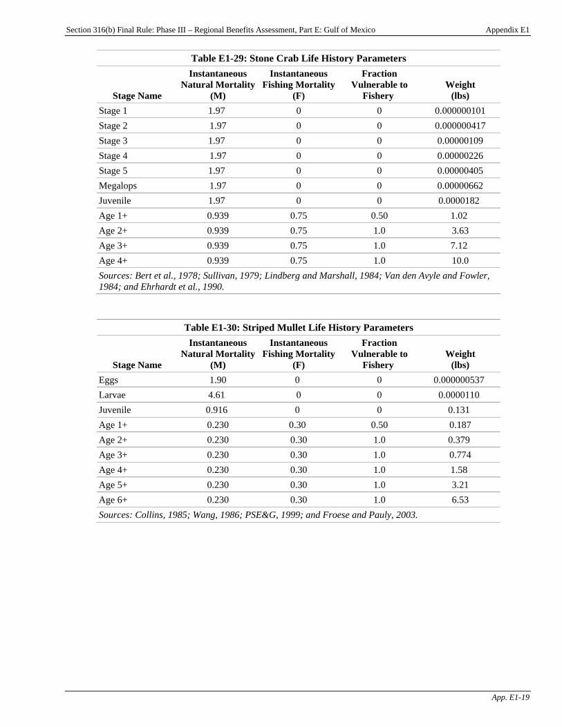
Section 316(b) Final Rule: Phase III – Regional Benefits Assessment, Part E: Gulf of Mexico Appendix E1
App. E1-19
Table E1-29: Stone Crab Life History Parameters
Stage Name
Instantaneous Natural Mortality
(M)
Instantaneous Fishing Mortality
(F)
Fraction Vulnerable to
FisheryP
P
Weight (lbs)
Stage 1 1.97P
P 0 0 0.000000101
Stage 2 1.97 0 0 0.000000417 Stage 3 1.97P
P 0 0 0.00000109
Stage 4 1.97 0 0 0.00000226 Stage 5 1.97P
P 0 0 0.00000405
Megalops 1.97 0 0 0.00000662 Juvenile 1.97P
P 0 0 0.0000182P
P
Age 1+ 0.939 0.75 0.50 1.02P
P
Age 2+ 0.939 0.75 1.0 3.63 Age 3+ 0.939 0.75 1.0 7.12P
P
Age 4+ 0.939 0.75 1.0 10.0 Sources: Bert et al., 1978; Sullivan, 1979; Lindberg and Marshall, 1984; Van den Avyle and Fowler, 1984; and Ehrhardt et al., 1990.
Table E1-30: Striped Mullet Life History Parameters
Stage Name
Instantaneous Natural Mortality
(M)
Instantaneous Fishing Mortality
(F)
Fraction Vulnerable to
FisheryP
P
Weight (lbs)
Eggs 1.90 0P
P 0 0.000000537P
P
Larvae 4.61P
P 0 0 0.0000110P
P
Juvenile 0.916P
P 0P
P 0 0.131P
P
Age 1+ 0.230 0.30P
P 0.50 0.187
Age 2+ 0.230 0.30 1.0 0.379P
P
Age 3+ 0.230 0.30 1.0 0.774 Age 4+ 0.230 0.30 1.0 1.58P
P
Age 5+ 0.230 0.30 1.0 3.21 Age 6+ 0.230 0.30 1.0 6.53 Sources: Collins, 1985; Wang, 1986; PSE&G, 1999; and Froese and Pauly, 2003.

Section 316(b) Final Rule: Phase III – Regional Benefits Assessment, Part E: Gulf of Mexico Appendix E1
App. E1-20
Table E1-31: Other Commercial Species Life History ParametersP
aP
Stage Name
Instantaneous Natural Mortality
(M)
Instantaneous Fishing Mortality
(F)
Fraction Vulnerable to
Fishery Weight
(lbs) Eggs 2.08 0 0 0.000000716 Larvae 5.71 0 0 0.00000204 Juvenile 2.85 0 0 0.000746 Age 1+ 0.450 0 0 0.0937 Age 2+ 0.450 0.80 0.50 0.356 Age 3+ 0.450 0.80 1.0 0.679 Age 4+ 0.450 0.80 1.0 0.974 Age 5+ 0.450 0.80 1.0 1.21 Age 6+ 0.450 0.80 1.0 1.38 P
aP Includes Atlantic cutlassfish, black bullhead, cobia, grey snapper, gulf butterfish, ladyfish, largehead
hairtail, mojarra spp., silver jenny, spotfin mojarra, tripletail, and yellow bullhead. Sources: USFWS, 1978; Durbin et al., 1983; Ruppert et al., 1985; Able and Fahay, 1998; PSE&G, 1999; Entergy Nuclear Generation Company, 2000; and ASMFC, 2001b.
Table E1-32: Other Recreational Species Life History ParametersP
aP
Stage Name
Instantaneous Natural Mortality
(M)
Instantaneous Fishing Mortality
(F)
Fraction Vulnerable to
Fishery Weight
(lbs) Eggs 2.08 0 0 0.000000716 Larvae 5.71 0 0 0.00000204 Juvenile 2.85 0 0 0.000746 Age 1+ 0.450 0 0 0.0937 Age 2+ 0.450 0.80 0.50 0.356 Age 3+ 0.450 0.80 1.0 0.679 Age 4+ 0.450 0.80 1.0 0.974 Age 5+ 0.450 0.80 1.0 1.21 Age 6+ 0.450 0.80 1.0 1.38 P
aP See Table E1-34 for a list of species.
Sources: USFWS, 1978; Durbin et al., 1983; Ruppert et al., 1985; Able and Fahay, 1998; PSE&G, 1999; Entergy Nuclear Generation Company, 2000; and ASMFC, 2001b.

Section 316(b) Final Rule: Phase III – Regional Benefits Assessment, Part E: Gulf of Mexico Appendix E1
App. E1-21
Table E1-33: Other Forage Species Life History ParametersP
aP
Stage Name
Instantaneous Natural Mortality
(M)
Instantaneous Fishing Mortality
(F)
Fraction Vulnerable to
FisheryP
P
Weight (lbs)
Eggs 1.04 0 0 0.0000000186 Larvae 7.70 0 0 0.00000158 Juvenile 1.29 0 0 0.000481 Age 1+ 1.62 0 0 0.00381 Age 2+ 1.62 0 0 0.00496P
P
Age 3+ 1.62 0 0 0.00505 P
aP See Table E1-35 for a list of species.
Sources: Derickson and Price, 1973; and PSE&G, 1999.
Table E1-34: Other Recreational SpeciesP
aP
Atlantic sharpnose shark Bonnethead Hardhead sea catfish Smooth butterfly ray Atlantic stingray Channel catfish Least puffer Smooth puffer Bandtail puffer Dwarf sandperch Pigfish Southern flounder Belted sandfish Gafftopsail catfish Rock sea bass Southern puffer Blackear bass Gag grouper Sand perch Tomtate Bluefish Gulf toadfish Sea catfish P
aP Includes other organisms not identified to species.
Table E1-35: Other Forage SpeciesP
aP
Atlantic midshipman Dwarf seahorse Jawfish Seahorse Atlantic needlefish Fat sleeper Lined seahorse Sheepshead minnow Atlantic spadefish Feather blenny Live sharksucker Snakefish Atlantic threadfin Florida blenny Longear sunfish Southern codling Barbfish Freckled blenny Mottled jawfish Southern hake Bay whiff Fringed filefish Needlefish Southern stargazer Blackcheek tonguefish Fringed flounder Orange filefish Spotted whiff Blackwing flyingfish Golden shiner Planehead filefish Striped blenny Bluegill Green sunfish Polka dot batfish Striped burrfish Bridle cardinalfish Gulf of Mexico ocellated flounder Redfin needlefish Warmouth Carp Halfbeak Roughback batfish Yellowhead jawfish Common halfbeak Harvestfish Sailfin molly Diamond lizardfish Inshore lizardfish Scrawled cowfish
P
aP Includes other organisms not identified to species.
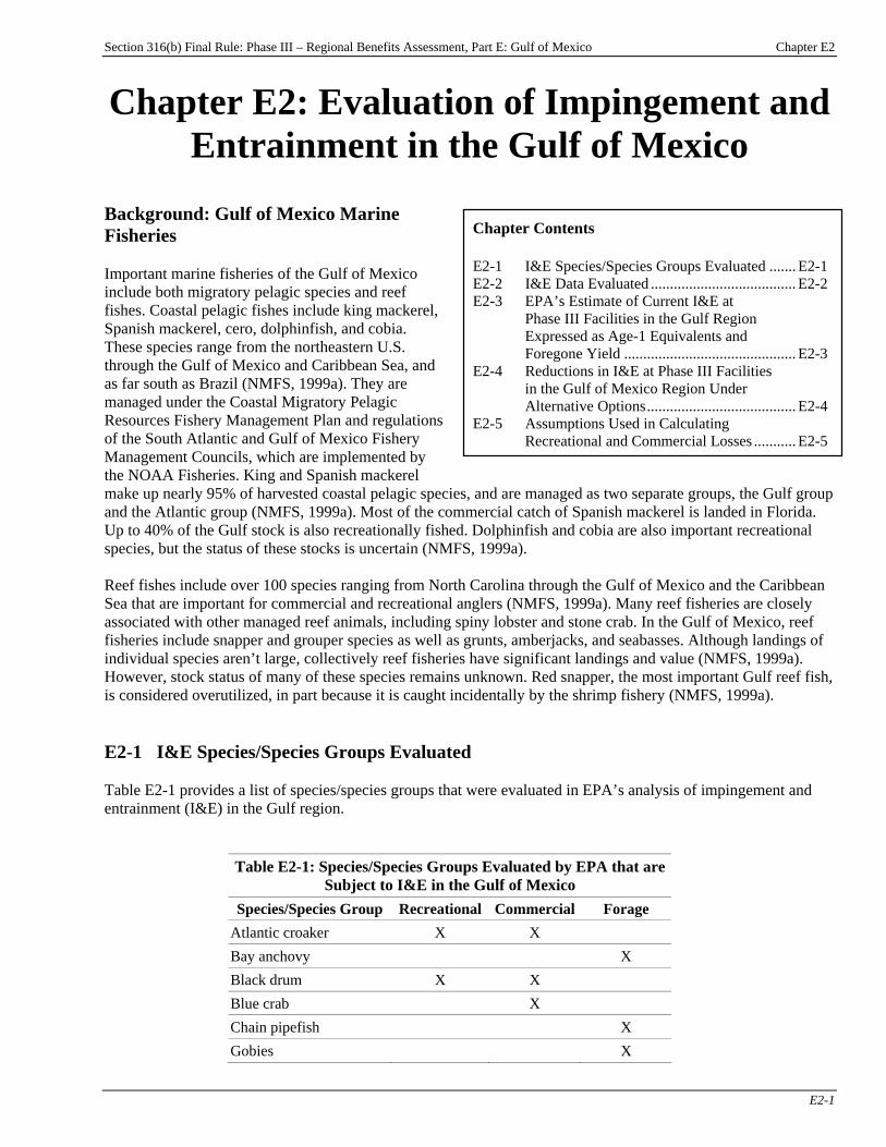
Section 316(b) Final Rule: Phase III – Regional Benefits Assessment, Part E: Gulf of Mexico Chapter E2
E2-1
Chapter E2: Evaluation of Impingement and Entrainment in the Gulf of Mexico
Background: Gulf of Mexico Marine Fisheries Important marine fisheries of the Gulf of Mexico include both migratory pelagic species and reef fishes. Coastal pelagic fishes include king mackerel, Spanish mackerel, cero, dolphinfish, and cobia. These species range from the northeastern U.S. through the Gulf of Mexico and Caribbean Sea, and as far south as Brazil (NMFS, 1999a). They are managed under the Coastal Migratory Pelagic Resources Fishery Management Plan and regulations of the South Atlantic and Gulf of Mexico Fishery Management Councils, which are implemented by the NOAA Fisheries. King and Spanish mackerel make up nearly 95% of harvested coastal pelagic species, and are managed as two separate groups, the Gulf group and the Atlantic group (NMFS, 1999a). Most of the commercial catch of Spanish mackerel is landed in Florida. Up to 40% of the Gulf stock is also recreationally fished. Dolphinfish and cobia are also important recreational species, but the status of these stocks is uncertain (NMFS, 1999a). Reef fishes include over 100 species ranging from North Carolina through the Gulf of Mexico and the Caribbean Sea that are important for commercial and recreational anglers (NMFS, 1999a). Many reef fisheries are closely associated with other managed reef animals, including spiny lobster and stone crab. In the Gulf of Mexico, reef fisheries include snapper and grouper species as well as grunts, amberjacks, and seabasses. Although landings of individual species aren’t large, collectively reef fisheries have significant landings and value (NMFS, 1999a). However, stock status of many of these species remains unknown. Red snapper, the most important Gulf reef fish, is considered overutilized, in part because it is caught incidentally by the shrimp fishery (NMFS, 1999a). E2-1 I&E Species/Species Groups Evaluated Table E2-1 provides a list of species/species groups that were evaluated in EPA’s analysis of impingement and entrainment (I&E) in the Gulf region.
Table E2-1: Species/Species Groups Evaluated by EPA that are Subject to I&E in the Gulf of Mexico
Species/Species Group Recreational Commercial Forage Atlantic croaker X X Bay anchovy X Black drum X X Blue crab X Chain pipefish X Gobies X
Chapter Contents E2-1 I&E Species/Species Groups Evaluated ....... E2-1 E2-2 I&E Data Evaluated ...................................... E2-2 E2-3 EPA’s Estimate of Current I&E at Phase III Facilities in the Gulf Region Expressed as Age-1 Equivalents and Foregone Yield ............................................. E2-3 E2-4 Reductions in I&E at Phase III Facilities in the Gulf of Mexico Region Under Alternative Options....................................... E2-4 E2-5 Assumptions Used in Calculating
Recreational and Commercial Losses ........... E2-5
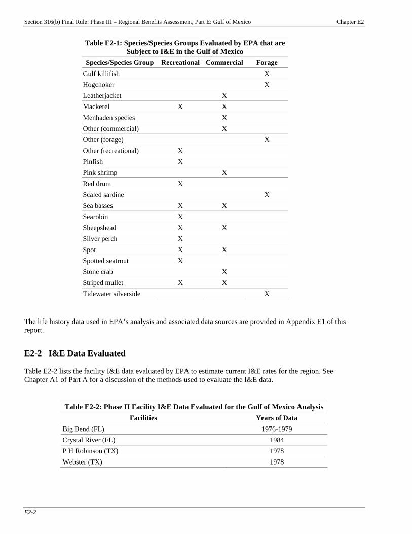
Section 316(b) Final Rule: Phase III – Regional Benefits Assessment, Part E: Gulf of Mexico Chapter E2
E2-2
Table E2-1: Species/Species Groups Evaluated by EPA that are Subject to I&E in the Gulf of Mexico
Species/Species Group Recreational Commercial Forage Gulf killifish X Hogchoker X Leatherjacket X Mackerel X X Menhaden species X Other (commercial) X Other (forage) X Other (recreational) X Pinfish X Pink shrimp X Red drum X Scaled sardine X Sea basses X X Searobin X Sheepshead X X Silver perch X Spot X X Spotted seatrout X Stone crab X Striped mullet X X Tidewater silverside X
The life history data used in EPA’s analysis and associated data sources are provided in Appendix E1 of this report. E2-2 I&E Data Evaluated Table E2-2 lists the facility I&E data evaluated by EPA to estimate current I&E rates for the region. See Chapter A1 of Part A for a discussion of the methods used to evaluate the I&E data.
Table E2-2: Phase II Facility I&E Data Evaluated for the Gulf of Mexico Analysis Facilities Years of Data
Big Bend (FL) 1976-1979 Crystal River (FL) 1984 P H Robinson (TX) 1978 Webster (TX) 1978
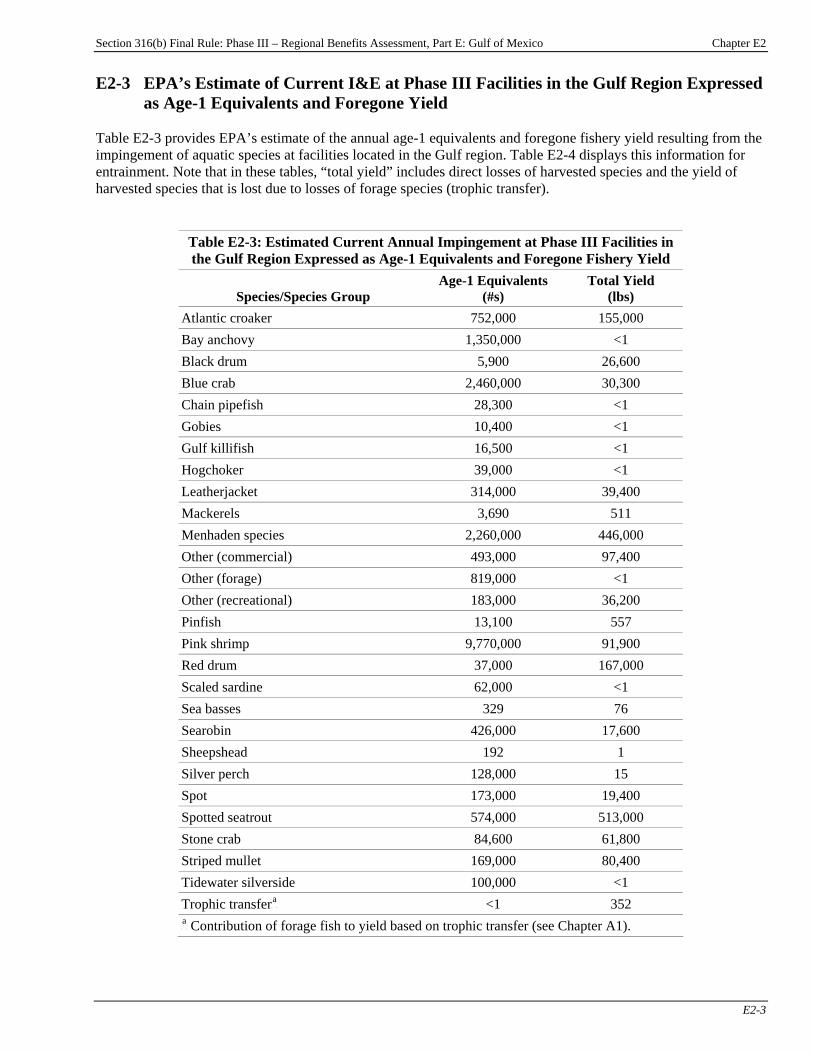
Section 316(b) Final Rule: Phase III – Regional Benefits Assessment, Part E: Gulf of Mexico Chapter E2
E2-3
E2-3 EPA’s Estimate of Current I&E at Phase III Facilities in the Gulf Region Expressed as Age-1 Equivalents and Foregone Yield
Table E2-3 provides EPA’s estimate of the annual age-1 equivalents and foregone fishery yield resulting from the impingement of aquatic species at facilities located in the Gulf region. Table E2-4 displays this information for entrainment. Note that in these tables, “total yield” includes direct losses of harvested species and the yield of harvested species that is lost due to losses of forage species (trophic transfer).
Table E2-3: Estimated Current Annual Impingement at Phase III Facilities in the Gulf Region Expressed as Age-1 Equivalents and Foregone Fishery Yield
Species/Species Group Age-1 Equivalents
(#s) Total Yield
(lbs) Atlantic croaker 752,000 155,000 Bay anchovy 1,350,000 <1 Black drum 5,900 26,600 Blue crab 2,460,000 30,300 Chain pipefish 28,300 <1 Gobies 10,400 <1 Gulf killifish 16,500 <1 Hogchoker 39,000 <1 Leatherjacket 314,000 39,400 Mackerels 3,690 511 Menhaden species 2,260,000 446,000 Other (commercial) 493,000 97,400 Other (forage) 819,000 <1 Other (recreational) 183,000 36,200 Pinfish 13,100 557 Pink shrimp 9,770,000 91,900 Red drum 37,000 167,000 Scaled sardine 62,000 <1 Sea basses 329 76 Searobin 426,000 17,600 Sheepshead 192 1 Silver perch 128,000 15 Spot 173,000 19,400 Spotted seatrout 574,000 513,000 Stone crab 84,600 61,800 Striped mullet 169,000 80,400 Tidewater silverside 100,000 <1 Trophic transferP
aP <1 352
P
aP Contribution of forage fish to yield based on trophic transfer (see Chapter A1).
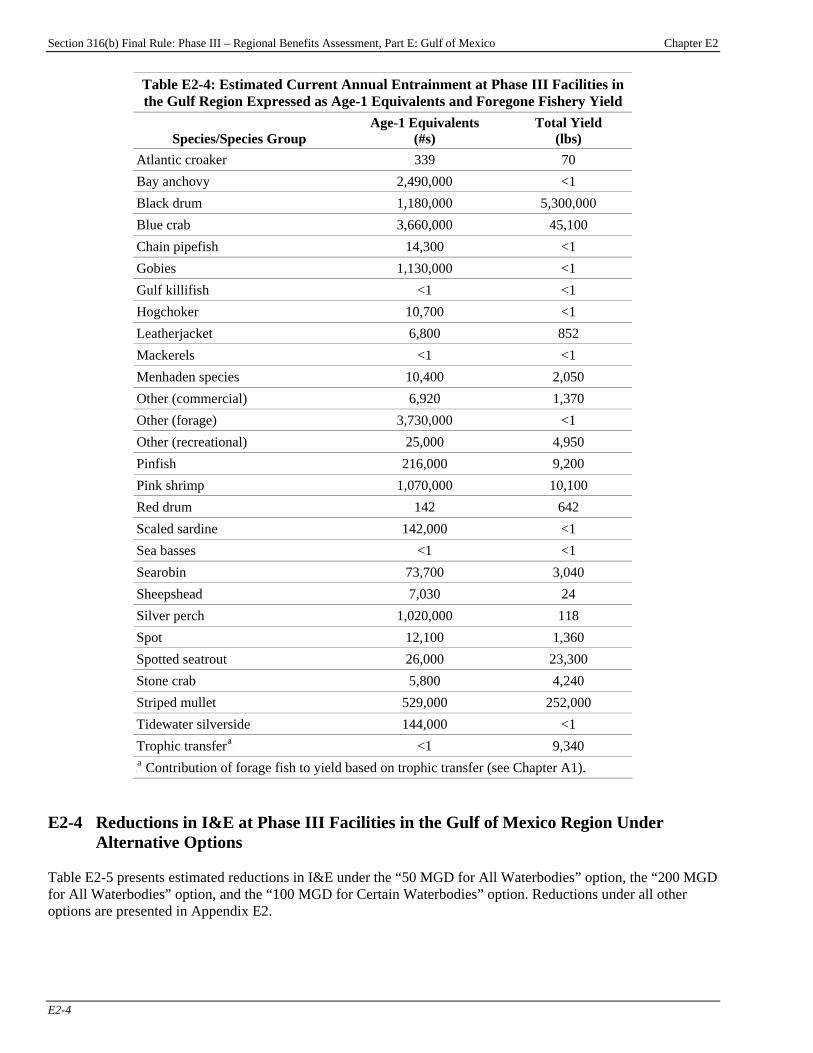
Section 316(b) Final Rule: Phase III – Regional Benefits Assessment, Part E: Gulf of Mexico Chapter E2
E2-4
Table E2-4: Estimated Current Annual Entrainment at Phase III Facilities in the Gulf Region Expressed as Age-1 Equivalents and Foregone Fishery Yield
Species/Species Group Age-1 Equivalents
(#s) Total Yield
(lbs) Atlantic croaker 339 70 Bay anchovy 2,490,000 <1 Black drum 1,180,000 5,300,000 Blue crab 3,660,000 45,100 Chain pipefish 14,300 <1 Gobies 1,130,000 <1 Gulf killifish <1 <1 Hogchoker 10,700 <1 Leatherjacket 6,800 852 Mackerels <1 <1 Menhaden species 10,400 2,050 Other (commercial) 6,920 1,370 Other (forage) 3,730,000 <1 Other (recreational) 25,000 4,950 Pinfish 216,000 9,200 Pink shrimp 1,070,000 10,100 Red drum 142 642 Scaled sardine 142,000 <1 Sea basses <1 <1 Searobin 73,700 3,040 Sheepshead 7,030 24 Silver perch 1,020,000 118 Spot 12,100 1,360 Spotted seatrout 26,000 23,300 Stone crab 5,800 4,240 Striped mullet 529,000 252,000 Tidewater silverside 144,000 <1 Trophic transferP
aP <1 9,340
P
aP Contribution of forage fish to yield based on trophic transfer (see Chapter A1).
E2-4 Reductions in I&E at Phase III Facilities in the Gulf of Mexico Region Under
Alternative Options Table E2-5 presents estimated reductions in I&E under the “50 MGD for All Waterbodies” option, the “200 MGD for All Waterbodies” option, and the “100 MGD for Certain Waterbodies” option. Reductions under all other options are presented in Appendix E2.
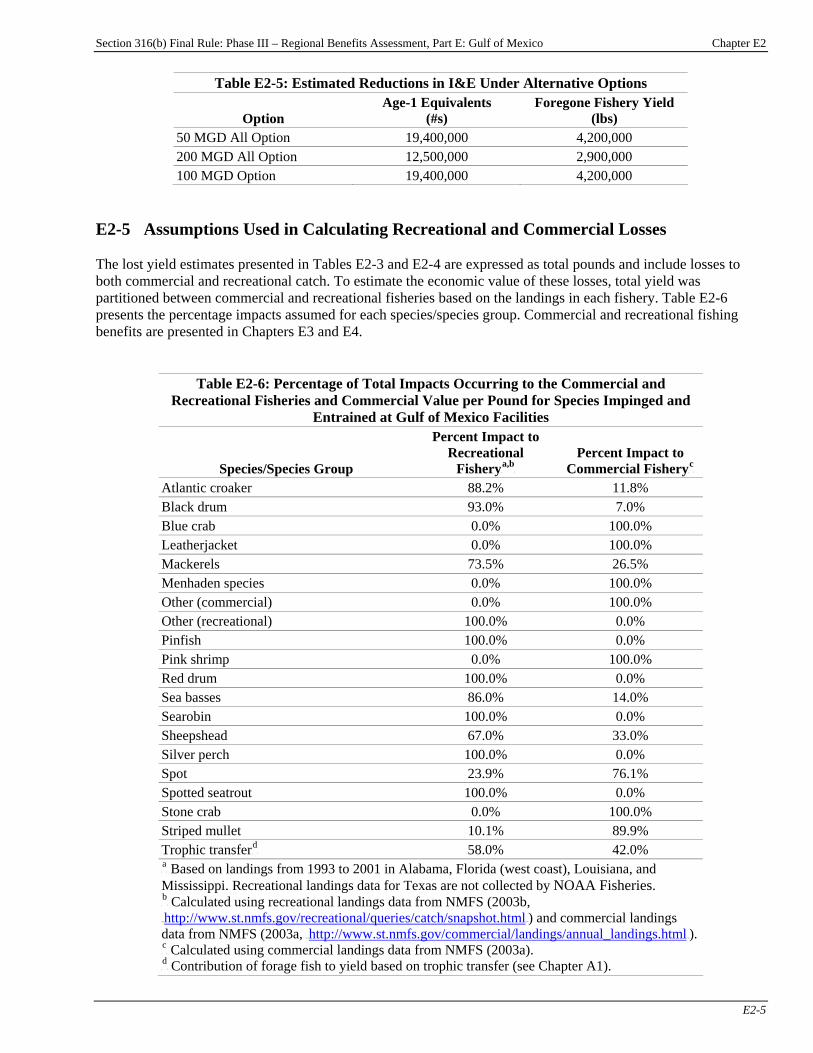
Section 316(b) Final Rule: Phase III – Regional Benefits Assessment, Part E: Gulf of Mexico Chapter E2
E2-5
Table E2-5: Estimated Reductions in I&E Under Alternative Options
Option Age-1 Equivalents
(#s) Foregone Fishery Yield
(lbs) 50 MGD All Option 19,400,000 4,200,000 200 MGD All Option 12,500,000 2,900,000 100 MGD Option 19,400,000 4,200,000
E2-5 Assumptions Used in Calculating Recreational and Commercial Losses The lost yield estimates presented in Tables E2-3 and E2-4 are expressed as total pounds and include losses to both commercial and recreational catch. To estimate the economic value of these losses, total yield was partitioned between commercial and recreational fisheries based on the landings in each fishery. Table E2-6 presents the percentage impacts assumed for each species/species group. Commercial and recreational fishing benefits are presented in Chapters E3 and E4.
Table E2-6: Percentage of Total Impacts Occurring to the Commercial and Recreational Fisheries and Commercial Value per Pound for Species Impinged and
Entrained at Gulf of Mexico Facilities
Species/Species Group
Percent Impact to Recreational
FisheryP
a,bP
Percent Impact to Commercial FisheryP
cP
Atlantic croaker 88.2% 11.8% Black drum 93.0% 7.0% Blue crab 0.0% 100.0% Leatherjacket 0.0% 100.0% Mackerels 73.5% 26.5% Menhaden species 0.0% 100.0% Other (commercial) 0.0% 100.0% Other (recreational) 100.0% 0.0% Pinfish 100.0% 0.0% Pink shrimp 0.0% 100.0% Red drum 100.0% 0.0% Sea basses 86.0% 14.0% Searobin 100.0% 0.0% Sheepshead 67.0% 33.0% Silver perch 100.0% 0.0% Spot 23.9% 76.1% Spotted seatrout 100.0% 0.0% Stone crab 0.0% 100.0% Striped mullet 10.1% 89.9% Trophic transferP
dP 58.0% 42.0%
P
aP Based on landings from 1993 to 2001 in Alabama, Florida (west coast), Louisiana, and
Mississippi. Recreational landings data for Texas are not collected by NOAA Fisheries. P
bP Calculated using recreational landings data from NMFS (2003b,
HTUhttp://www.st.nmfs.gov/recreational/queries/catch/snapshot.htmlUTH) and commercial landings data from NMFS (2003a, HTUhttp://www.st.nmfs.gov/commercial/landings/annual_landings.htmlUTH).P
cP Calculated using commercial landings data from NMFS (2003a).
P
dP Contribution of forage fish to yield based on trophic transfer (see Chapter A1).

Section 316(b) Final Rule: Phase III – Regional Benefits Assessment, Part E: Gulf of Mexico Chapter E2
E2-6
See Chapter E3 for results of the commercial fishing benefits analysis and Chapter E4 for recreational fishing results. As discussed in Chapter A8, benefits were discounted to account for (1) the time to achieve compliance once a Phase III final regulation for existing facilities would have become effective, and (2) the time it takes for fish spared from I&E to reach a harvestable age.

Section 316(b) Final Rule: Phase III – Regional Benefits Assessment, Part E: Gulf of Mexico Appendix E2
App. E2-1
Appendix E2: Reductions in I&E Under Supplemental Policy Options
Table E2-1: Estimated Reductions in I&E in the Gulf of Mexico Region Under Eight Supplemental Options
Option Age-1 Equivalents
(#s) Foregone Fishery Yield
(lbs) Electric Generators 2-50 MGD
I-only Everywhere 0 0 I&E like Phase II 0 0 I&E Everywhere 0 0
Manufacturers 2-50 MGD I-only Everywhere 543,000 47,800 I&E like Phase II 855,000 162,000 I&E Everywhere 855,000 162,000
Manufacturers 50+ MGD I-only Everywhere 10,400,000 917,000 I&E Everywhere 19,400,000 4,200,000
Section 316(b) Final Rule: Phase III – Regional Benefits Assessment, Part E: Gulf of Mexico Chapter E3
E3-1
Chapter E3: Commercial Fishing Benefits Introduction
Chapter Contents E3-1 Baseline Commercial Losses ........................ E3-1 E3-2 Expected Benefits Under Regulatory Analysis Options........................................... E3-3
E3-2.1 Commercial Fishing Benefits of the “50 MGD for All Waterbodies” Option.............................................. E3-3 E3-2.2 Commercial Fishing Benefits of the “200 MGD for All Waterbodies” Option.............................................. E3-4
E3-2.3 Commercial Fishing Benefits of the “100 MGD for Certain Waterbodies” Option....................... E3-4
This chapter presents the results of the commercial fishing benefits analysis for the Gulf of Mexico region. The chapter presents EPA’s estimates of baseline (i.e., current) annual commercial fishery losses from impingement and entrainment (I&E) at potentially regulated facilities in the Gulf of Mexico region and annual reductions in these losses under the regulatory options for Phase III existing facilitiesPF
1FP:
< the “50 MGD for All Waterbodies” option, < the “200 MGD for All Waterbodies” option,
and < the “100 MGD for Certain Waterbodies”
option. The chapter then presents the estimated benefits to commercial fisheries from eliminating baseline losses from I&E, and the expected benefits under the regulatory options. Chapter A4, “Methods for Estimating Commercial Fishing Benefits,” details the methods used by EPA to estimate the commercial fishing benefits of reducing and eliminating I&E losses. EPA considered a wide range of policy options in developing this regulation. In addition to the regulatory options, EPA evaluated several supplemental options. Appendix E3 presents results of the commercial fishing benefits analysis for the supplemental options. For additional information on the options, please see the TDD. E3-1 Baseline Commercial Losses Table E3-1 provides EPA’s estimate of the value of gross revenues lost in commercial fisheries resulting from the impingement of aquatic species at facilities in the Gulf of Mexico region. Table E3-2 displays this information for entrainment. Total annualized revenue losses are approximately $1,020,218 (undiscounted).
P
1P See the Introduction to this report for a description of the primary analysis options.
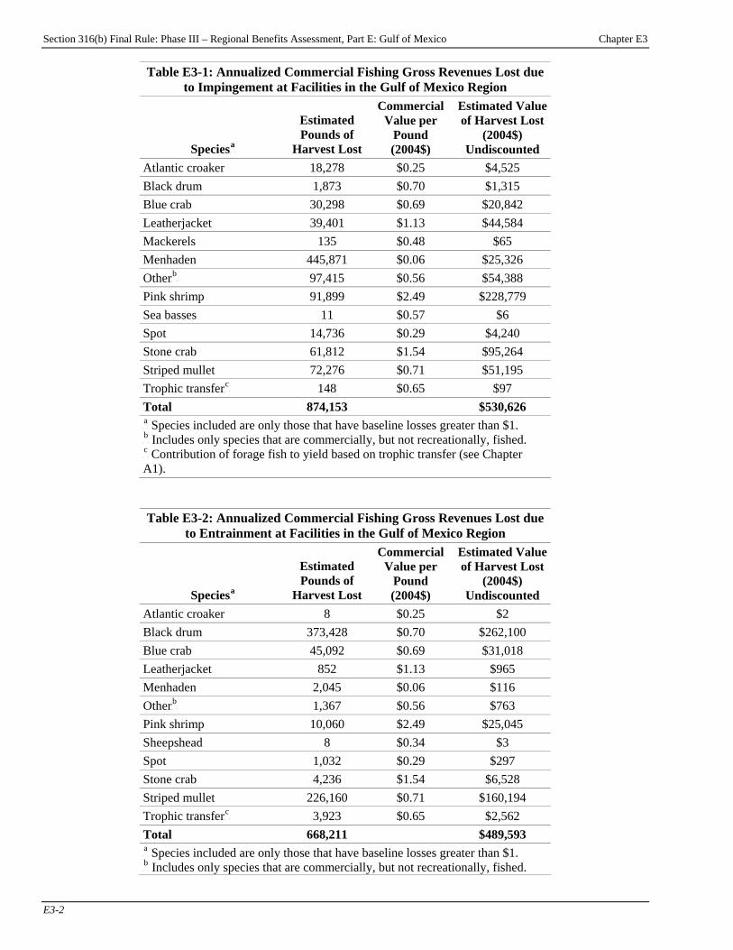
Section 316(b) Final Rule: Phase III – Regional Benefits Assessment, Part E: Gulf of Mexico Chapter E3
E3-2
Table E3-1: Annualized Commercial Fishing Gross Revenues Lost due to Impingement at Facilities in the Gulf of Mexico Region
SpeciesP
aP
Estimated Pounds of
Harvest Lost
Commercial Value per
Pound (2004$)
Estimated Value of Harvest Lost
(2004$) Undiscounted
Atlantic croaker 18,278 $0.25 $4,525 Black drum 1,873 $0.70 $1,315 Blue crab 30,298 $0.69 $20,842 Leatherjacket 39,401 $1.13 $44,584 Mackerels 135 $0.48 $65 Menhaden 445,871 $0.06 $25,326 OtherP
bP 97,415 $0.56 $54,388
Pink shrimp 91,899 $2.49 $228,779 Sea basses 11 $0.57 $6 Spot 14,736 $0.29 $4,240 Stone crab 61,812 $1.54 $95,264 Striped mullet 72,276 $0.71 $51,195 Trophic transferP
cP 148 $0.65 $97
Total 874,153 $530,626 P
aP Species included are only those that have baseline losses greater than $1.
P
bP Includes only species that are commercially, but not recreationally, fished.
P
cP Contribution of forage fish to yield based on trophic transfer (see Chapter
A1).
Table E3-2: Annualized Commercial Fishing Gross Revenues Lost due to Entrainment at Facilities in the Gulf of Mexico Region
SpeciesP
aP
Estimated Pounds of
Harvest Lost
Commercial Value per
Pound (2004$)
Estimated Value of Harvest Lost
(2004$) Undiscounted
Atlantic croaker 8 $0.25 $2 Black drum 373,428 $0.70 $262,100 Blue crab 45,092 $0.69 $31,018 Leatherjacket 852 $1.13 $965 Menhaden 2,045 $0.06 $116 OtherP
bP 1,367 $0.56 $763
Pink shrimp 10,060 $2.49 $25,045 Sheepshead 8 $0.34 $3 Spot 1,032 $0.29 $297 Stone crab 4,236 $1.54 $6,528 Striped mullet 226,160 $0.71 $160,194 Trophic transferP
cP 3,923 $0.65 $2,562
Total 668,211 $489,593 P
aP Species included are only those that have baseline losses greater than $1.
P
bP Includes only species that are commercially, but not recreationally, fished.

Section 316(b) Final Rule: Phase III – Regional Benefits Assessment, Part E: Gulf of Mexico Chapter E3
E3-3
Table E3-2: Annualized Commercial Fishing Gross Revenues Lost due to Entrainment at Facilities in the Gulf of Mexico Region
SpeciesP
aP
Estimated Pounds of
Harvest Lost
Commercial Value per
Pound (2004$)
Estimated Value of Harvest Lost
(2004$) Undiscounted
P
cP Contribution of forage fish to yield based on trophic transfer (see Chapter
A1). E3-2 Expected Benefits Under Regulatory Analysis Options As described in Chapter A4, EPA estimates for Gulf of Mexico that, depending on species, 0 to 79% of the gross revenue losses represent surplus losses to producers, assuming no change in prices or fishing costs. Earlier EPA analysis assumed a rate of 40%. The 0% estimate, of course, results in loss estimates of $0. The expected reductions in I&E attributable to changes at facilities required by the “50 MGD for All Waterbodies” option (50 MGD All option) are 51.4% for impingement and 57.9% for entrainment; the expected reductions for the “200 MGD for All Waterbodies” option (200 MGD All option) are 29.9% for impingement and 41.8% for entrainment; and the expected reductions for the “100 MGD for Certain Waterbodies” option (100 MGD CWB option) are 51.4% for impingement and 57.9% for entrainment. Total annualized benefits are estimated by applying these estimated reductions to the annual baseline producer surplus loss. As presented in Tables E3-3, E3-4, and E3-5, this results in total annualized benefits of up to approximately $283,218 for the 50 MGD All option, $188,205 for the 200 MGD All option, and $283,218 for the 100 MGD CWB option, assuming a 3% discount rate and a species-specific net benefits ratio.TPF
2FPT
E3-2.1 Commercial Fishing Benefits of the “50 MGD for All Waterbodies” Option Table E3-3 shows EPA’s analysis of the commercial benefits of the “50 MGD for All Waterbodies” option for the Gulf of Mexico region. The table shows that this option, assuming a species-specific net benefits ratio, will result in undiscounted total annualized commercial benefits of approximately $338,493. When evaluated at 3% and 7% discount rates, the annualized commercial benefits are $283,218 and $225,425, respectively.
Table E3-3: Annualized Commercial Fishing Benefits Attributable to the 50 MGD All Option at Facilities in the Gulf of Mexico Region (2004$)P
aP
Impingement Entrainment Total Baseline loss — gross revenue
Undiscounted $530,625 $489,593 $1,020,218 Producer surplus lost — 0% $0 $0 $0 Producer surplus lost — (gross revenue * species-specific net benefits ratio)
Undiscounted $267,680 $346,483 $614,163 Expected reduction due to rule 51.4% 57.9% Benefits attributable to rule — 0% $0 $0 $0 Benefits attributable to rule — species-specific net benefits ratio
Undiscounted $338,493 3% discount rate $283,218
TP
2PT The net benefits ratio is the fractional share of gross revenue associated with net benefits, by gear and vessel type.
See Chapter A4, section A4-10, for a description of the species-specific net benefits ratios and how they are calculated.

Section 316(b) Final Rule: Phase III – Regional Benefits Assessment, Part E: Gulf of Mexico Chapter E3
E3-4
7% discount rate $225,425 P
aP Annualized benefits represent the value of all commercial benefits generated over the time
frame of the analysis, discounted to 2007, and then annualized over a 30 year period. For a more detailed discussion of the discounting methodology, refer to Chapter A8, and see Chapter I1 for a timeline of benefits.
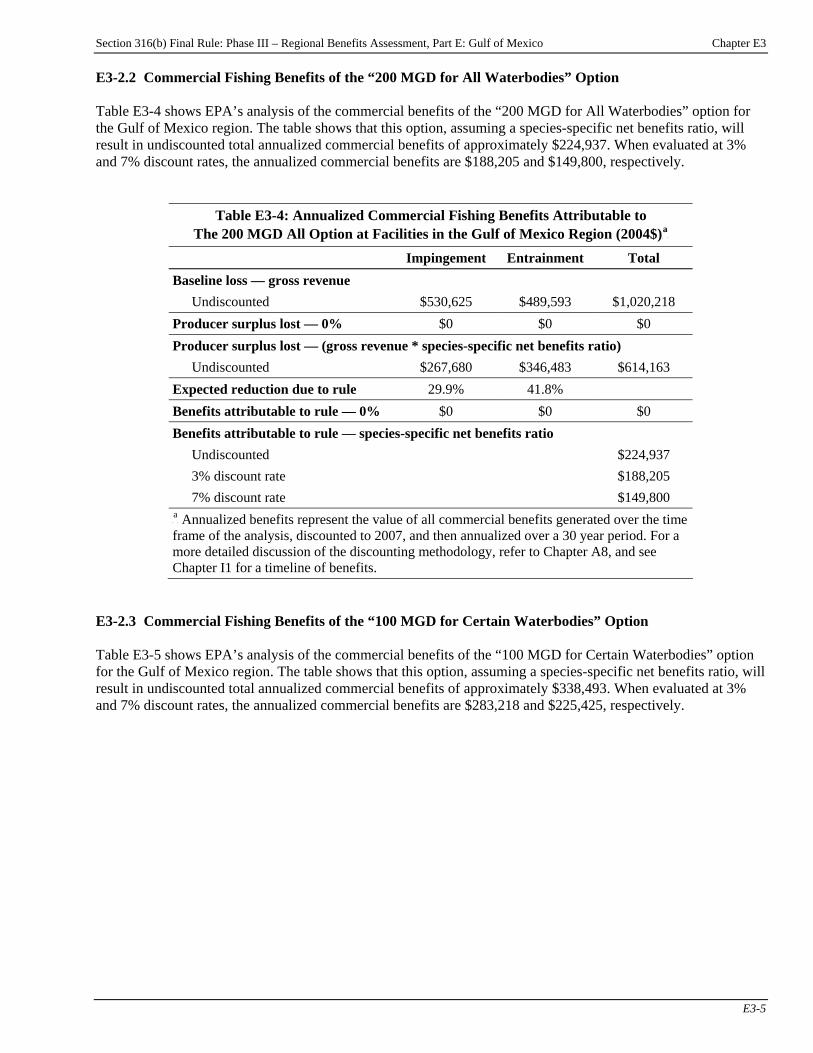
Section 316(b) Final Rule: Phase III – Regional Benefits Assessment, Part E: Gulf of Mexico Chapter E3
E3-5
E3-2.2 Commercial Fishing Benefits of the “200 MGD for All Waterbodies” Option Table E3-4 shows EPA’s analysis of the commercial benefits of the “200 MGD for All Waterbodies” option for the Gulf of Mexico region. The table shows that this option, assuming a species-specific net benefits ratio, will result in undiscounted total annualized commercial benefits of approximately $224,937. When evaluated at 3% and 7% discount rates, the annualized commercial benefits are $188,205 and $149,800, respectively.
Table E3-4: Annualized Commercial Fishing Benefits Attributable to The 200 MGD All Option at Facilities in the Gulf of Mexico Region (2004$)P
aP
Impingement Entrainment Total Baseline loss — gross revenue
Undiscounted $530,625 $489,593 $1,020,218 Producer surplus lost — 0% $0 $0 $0 Producer surplus lost — (gross revenue * species-specific net benefits ratio)
Undiscounted $267,680 $346,483 $614,163 Expected reduction due to rule 29.9% 41.8% Benefits attributable to rule — 0% $0 $0 $0 Benefits attributable to rule — species-specific net benefits ratio
Undiscounted $224,937 3% discount rate $188,205 7% discount rate $149,800
P
aP Annualized benefits represent the value of all commercial benefits generated over the time
frame of the analysis, discounted to 2007, and then annualized over a 30 year period. For a more detailed discussion of the discounting methodology, refer to Chapter A8, and see Chapter I1 for a timeline of benefits.
E3-2.3 Commercial Fishing Benefits of the “100 MGD for Certain Waterbodies” Option Table E3-5 shows EPA’s analysis of the commercial benefits of the “100 MGD for Certain Waterbodies” option for the Gulf of Mexico region. The table shows that this option, assuming a species-specific net benefits ratio, will result in undiscounted total annualized commercial benefits of approximately $338,493. When evaluated at 3% and 7% discount rates, the annualized commercial benefits are $283,218 and $225,425, respectively.
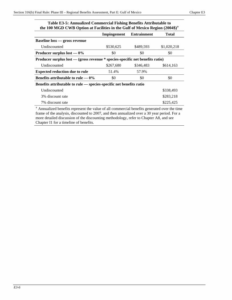
Section 316(b) Final Rule: Phase III – Regional Benefits Assessment, Part E: Gulf of Mexico Chapter E3
E3-6
Table E3-5: Annualized Commercial Fishing Benefits Attributable to the 100 MGD CWB Option at Facilities in the Gulf of Mexico Region (2004$)P
aP
Impingement Entrainment Total Baseline loss — gross revenue
Undiscounted $530,625 $489,593 $1,020,218 Producer surplus lost — 0% $0 $0 $0 Producer surplus lost — (gross revenue * species-specific net benefits ratio)
Undiscounted $267,680 $346,483 $614,163 Expected reduction due to rule 51.4% 57.9% Benefits attributable to rule — 0% $0 $0 $0 Benefits attributable to rule — species-specific net benefits ratio
Undiscounted $338,493 3% discount rate $283,218 7% discount rate $225,425
P
aP Annualized benefits represent the value of all commercial benefits generated over the time
frame of the analysis, discounted to 2007, and then annualized over a 30 year period. For a more detailed discussion of the discounting methodology, refer to Chapter A8, and see Chapter I1 for a timeline of benefits.
Section 316(b) Final Rule: Phase III – Regional Benefits Assessment, Part E: Gulf of Mexico Appendix E3
App. E3-1
Appendix E3: Commercial Fishing Benefits Under Supplemental Policy Options
Introduction Chapter E3 presents EPA’s estimates of the commercial benefits of the regulatory options for the section 316(b) rule for Phase III facilities in the Gulf of Mexico region. To facilitate comparisons among the options, this appendix presents estimates of the commercial fishing benefits of several supplemental options that EPA evaluated in preparation for this rule:
Appendix Contents E3-1 Commercial Fishing Benefits of the Supplemental Options .................................E3-2
< “Electric Generators 2-50 MGD I-only Everywhere” option; < “Electric Generators 2-50 MGD I&E like Phase II” option; < “Electric Generators 2-50 MGD I&E Everywhere” option; < “Manufacturers 2-50 MGD I-only Everywhere” option; < “Manufacturers 2-50 MGD I&E like Phase II” option; < “Manufacturers 2-50 MGD I&E Everywhere” option; < “Manufacturers 50+ MGD I-only Everywhere” option; and < “Manufacturers 50+ MGD I&E Everywhere” option.
Commercial fishing benefits presented in this chapter were estimated using the benefit transfer approach discussed in Chapter E3 and in Chapter A4, “Methods for Estimating Commercial Fishing Benefits.” For additional information on the options, please see the TDD.
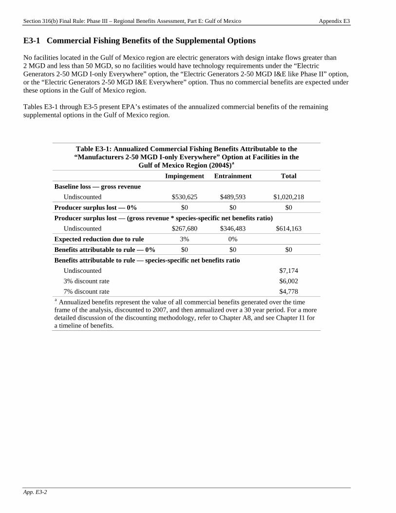
Section 316(b) Final Rule: Phase III – Regional Benefits Assessment, Part E: Gulf of Mexico Appendix E3
App. E3-2
E3-1 Commercial Fishing Benefits of the Supplemental Options No facilities located in the Gulf of Mexico region are electric generators with design intake flows greater than 2 MGD and less than 50 MGD, so no facilities would have technology requirements under the “Electric Generators 2-50 MGD I-only Everywhere” option, the “Electric Generators 2-50 MGD I&E like Phase II” option, or the “Electric Generators 2-50 MGD I&E Everywhere” option. Thus no commercial benefits are expected under these options in the Gulf of Mexico region. Tables E3-1 through E3-5 present EPA’s estimates of the annualized commercial benefits of the remaining supplemental options in the Gulf of Mexico region.
Table E3-1: Annualized Commercial Fishing Benefits Attributable to the “Manufacturers 2-50 MGD I-only Everywhere” Option at Facilities in the
Gulf of Mexico Region (2004$)P
aP
Impingement Entrainment Total Baseline loss — gross revenue
Undiscounted $530,625 $489,593 $1,020,218 Producer surplus lost — 0% $0 $0 $0 Producer surplus lost — (gross revenue * species-specific net benefits ratio)
Undiscounted $267,680 $346,483 $614,163 Expected reduction due to rule 3% 0% Benefits attributable to rule — 0% $0 $0 $0 Benefits attributable to rule — species-specific net benefits ratio
Undiscounted $7,174 3% discount rate $6,002 7% discount rate $4,778
P
aP Annualized benefits represent the value of all commercial benefits generated over the time
frame of the analysis, discounted to 2007, and then annualized over a 30 year period. For a more detailed discussion of the discounting methodology, refer to Chapter A8, and see Chapter I1 for a timeline of benefits.
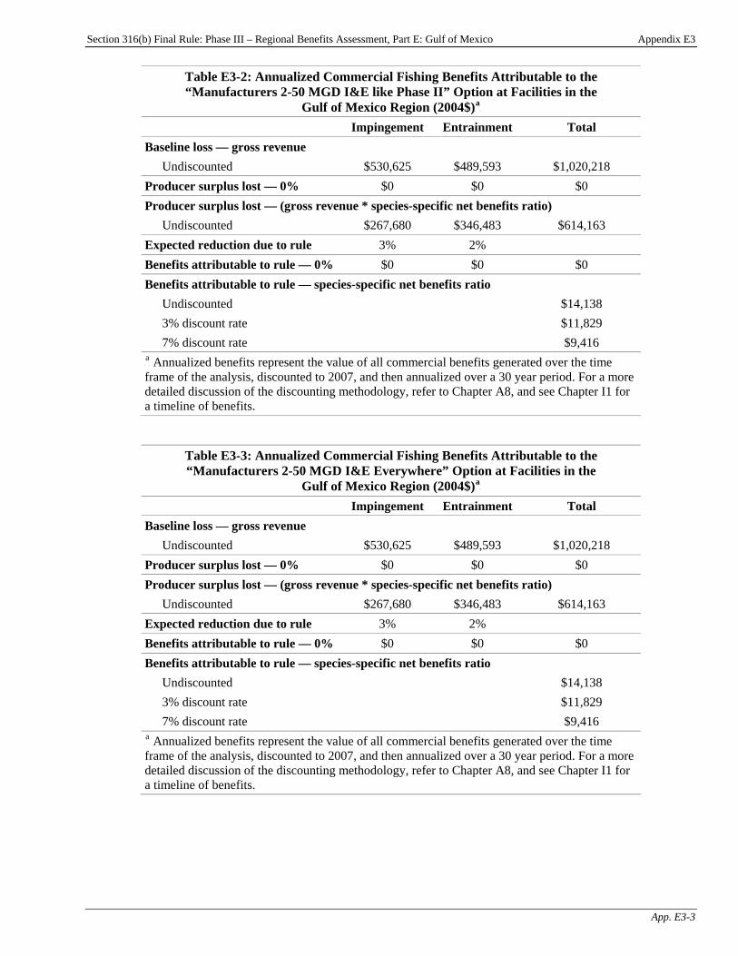
Section 316(b) Final Rule: Phase III – Regional Benefits Assessment, Part E: Gulf of Mexico Appendix E3
App. E3-3
Table E3-2: Annualized Commercial Fishing Benefits Attributable to the “Manufacturers 2-50 MGD I&E like Phase II” Option at Facilities in the
Gulf of Mexico Region (2004$)P
aP
Impingement Entrainment Total Baseline loss — gross revenue
Undiscounted $530,625 $489,593 $1,020,218 Producer surplus lost — 0% $0 $0 $0 Producer surplus lost — (gross revenue * species-specific net benefits ratio)
Undiscounted $267,680 $346,483 $614,163 Expected reduction due to rule 3% 2% Benefits attributable to rule — 0% $0 $0 $0 Benefits attributable to rule — species-specific net benefits ratio
Undiscounted $14,138 3% discount rate $11,829 7% discount rate $9,416
P
aP Annualized benefits represent the value of all commercial benefits generated over the time
frame of the analysis, discounted to 2007, and then annualized over a 30 year period. For a more detailed discussion of the discounting methodology, refer to Chapter A8, and see Chapter I1 for a timeline of benefits.
Table E3-3: Annualized Commercial Fishing Benefits Attributable to the “Manufacturers 2-50 MGD I&E Everywhere” Option at Facilities in the
Gulf of Mexico Region (2004$)P
aP
Impingement Entrainment Total Baseline loss — gross revenue
Undiscounted $530,625 $489,593 $1,020,218 Producer surplus lost — 0% $0 $0 $0 Producer surplus lost — (gross revenue * species-specific net benefits ratio)
Undiscounted $267,680 $346,483 $614,163 Expected reduction due to rule 3% 2% Benefits attributable to rule — 0% $0 $0 $0 Benefits attributable to rule — species-specific net benefits ratio
Undiscounted $14,138 3% discount rate $11,829 7% discount rate $9,416
P
aP Annualized benefits represent the value of all commercial benefits generated over the time
frame of the analysis, discounted to 2007, and then annualized over a 30 year period. For a more detailed discussion of the discounting methodology, refer to Chapter A8, and see Chapter I1 for a timeline of benefits.
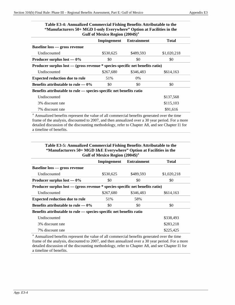
Section 316(b) Final Rule: Phase III – Regional Benefits Assessment, Part E: Gulf of Mexico Appendix E3
App. E3-4
Table E3-4: Annualized Commercial Fishing Benefits Attributable to the “Manufacturers 50+ MGD I-only Everywhere” Option at Facilities in the
Gulf of Mexico Region (2004$)P
aP
Impingement Entrainment Total Baseline loss — gross revenue
Undiscounted $530,625 $489,593 $1,020,218 Producer surplus lost — 0% $0 $0 $0 Producer surplus lost — (gross revenue * species-specific net benefits ratio)
Undiscounted $267,680 $346,483 $614,163 Expected reduction due to rule 51% 0% Benefits attributable to rule — 0% $0 $0 $0 Benefits attributable to rule — species-specific net benefits ratio
Undiscounted $137,568 3% discount rate $115,103 7% discount rate $91,616
P
aP Annualized benefits represent the value of all commercial benefits generated over the time
frame of the analysis, discounted to 2007, and then annualized over a 30 year period. For a more detailed discussion of the discounting methodology, refer to Chapter A8, and see Chapter I1 for a timeline of benefits.
Table E3-5: Annualized Commercial Fishing Benefits Attributable to the “Manufacturers 50+ MGD I&E Everywhere” Option at Facilities in the
Gulf of Mexico Region (2004$)P
aP
Impingement Entrainment Total Baseline loss — gross revenue
Undiscounted $530,625 $489,593 $1,020,218 Producer surplus lost — 0% $0 $0 $0 Producer surplus lost — (gross revenue * species-specific net benefits ratio)
Undiscounted $267,680 $346,483 $614,163 Expected reduction due to rule 51% 58% Benefits attributable to rule — 0% $0 $0 $0 Benefits attributable to rule — species-specific net benefits ratio
Undiscounted $338,493 3% discount rate $283,218 7% discount rate $225,425
P
aP Annualized benefits represent the value of all commercial benefits generated over the time
frame of the analysis, discounted to 2007, and then annualized over a 30 year period. For a more detailed discussion of the discounting methodology, refer to Chapter A8, and see Chapter I1 for a timeline of benefits.
Section 316(b) Final Rule: Phase III – Regional Benefits Assessment, Part E: Gulf of Mexico Chapter E4
E4-1
Chapter E4: Recreational Use Benefits Introduction
Chapter Contents E4-1 Benefit Transfer Approach Based on Meta- Analysis ........................................................ E4-1 E4-1.1 Baseline Losses and Reductions in Recreational Fishery Losses Under the Regulatory Options.................. E4-2 E4-1.2 Recreational Fishing Benefits from Eliminating Baseline I&E Losses ............................................. E4-3 E4-1.3 Recreational Fishing Benefits of the “50 MGD for All Waterbodies” Option ............................................. E4-4 E4-1.4 Recreational Fishing Benefits of the “200 MGD for All Waterbodies” Option ............................................. E4-5 E4-1.5 Recreational Fishing Benefits of the “100 MGD for Certain Waterbodies” Option ............................................. E4-6 E4-2 Limitations and Uncertainty ......................... E4-6
This chapter presents the results of the recreational fishing benefits analysis for the Gulf of Mexico region. The chapter presents EPA’s estimates of baseline (i.e., current) annual recreational fishery losses from impingement and entrainment (I&E) at potentially regulated facilities in the Gulf of Mexico region and annual reductions in these losses under the regulatory options for Phase III existing facilitiesPF
1FP:
< the “50 MGD for All Waterbodies” option, < the “200 MGD for All Waterbodies” option,
and < the “100 MGD for Certain Waterbodies”
option. The chapter then presents the estimated welfare gain to Gulf of Mexico anglers from eliminating baseline recreational fishing losses from I&E and the expected benefits under the regulatory options. EPA estimated the recreational benefits of reducing and eliminating I&E losses using a benefit transfer methodology based on a meta-analysis of the marginal value of catching different species of fish. This meta-analysis is discussed in detail in Chapter A5, “Recreational Fishing Benefits Methodology.” EPA considered a wide range of policy options in developing this regulation. In addition to the regulatory options, EPA evaluated several supplemental options. Appendix E4 presents results of the recreational fishing benefits analysis for the supplemental options. For additional information on the options, please see the TDD. E4-1 Benefit Transfer Approach Based on Meta-Analysis EPA estimated the recreational welfare gain from the reduction in annual I&E losses expected under the policy options, and the welfare gain from eliminating I&E at potentially regulated facilities, using a benefit transfer approach. As discussed in Chapter A5, the Agency used a meta-analysis regression equation to estimate the marginal recreational value per additional fish caught by anglers, for different species in different regions. Since I&E at potentially regulated facilities affects a variety of species, EPA assigned each species with I&E losses to one of the general species groups used in the meta-analysis. The Agency then calculated the economic value of reducing or eliminating baseline I&E losses, for each species group, by multiplying the value per fish for that species group by the number of fish in the group that are lost in the baseline or saved under the policy options.PF
2FP
P
1P See the Introduction to this report for a description of the regulatory options.
P
2P The estimates of I&E presented in this chapter include only the fraction of impinged and entrained recreational
fish that would be caught by anglers. The total amount of I&E of recreational species is actually much higher.
Section 316(b) Final Rule: Phase III – Regional Benefits Assessment, Part E: Gulf of Mexico Chapter E4
E4-2
In general, the fit between the species with I&E losses and the species groups in the meta-analysis was good. However, EPA’s estimates of baseline I&E losses and reductions in I&E under the policy options included losses of “unidentified” species. The “unidentified” group includes fish lost indirectly through trophic transfer, as well as species for which no species information was available.PF
3FP Rather than using the meta-analysis regression to try to
predict the value per fish for an “unidentified” species, EPA assumed that per-fish values for these species can be approximated by the weighted average value per fish for all species affected by I&E in the Gulf of Mexico region.PF
4FP
E4-1.1 Baseline Losses and Reductions in Recreational Fishery Losses Under the Regulatory Options Table E4-1 presents EPA’s estimates of baseline (i.e., current) annual recreational I&E losses at potentially regulated facilities, and annual reductions in these losses under each of the regulatory options, in the Gulf of Mexico region. The table shows that total baseline losses to recreational fisheries are 788.0 thousand fish per year. In comparison, the “50 MGD for All Waterbodies” and “100 MGD for Certain Waterbodies” options prevent losses of 430.9 thousand fish per year, and the “200 MGD for All Waterbodies” option prevents losses of 282.4 thousand fish per year. Of all the affected species, black drum and spotted seatrout have the highest losses in the baseline and the highest prevented losses under the regulatory options.
P
3P In addition to recreational fish that are lost because they are impinged or entrained, some recreational fish are lost
because the forage fish that they feed on are impinged or entrained, and thus removed from the food chain. These trophic transfer losses of recreational species are included in EPA’s estimates of total I&E losses. Since it is difficult to predict which recreational species would be affected by losses of forage fish, these losses are classified as “unidentified” recreational species. Also included in the “unidentified” group are losses of fish that were reported by facilities without information about their exact species.
P
4P EPA used the estimated level of baseline recreational losses for each species group as a weighting factor.
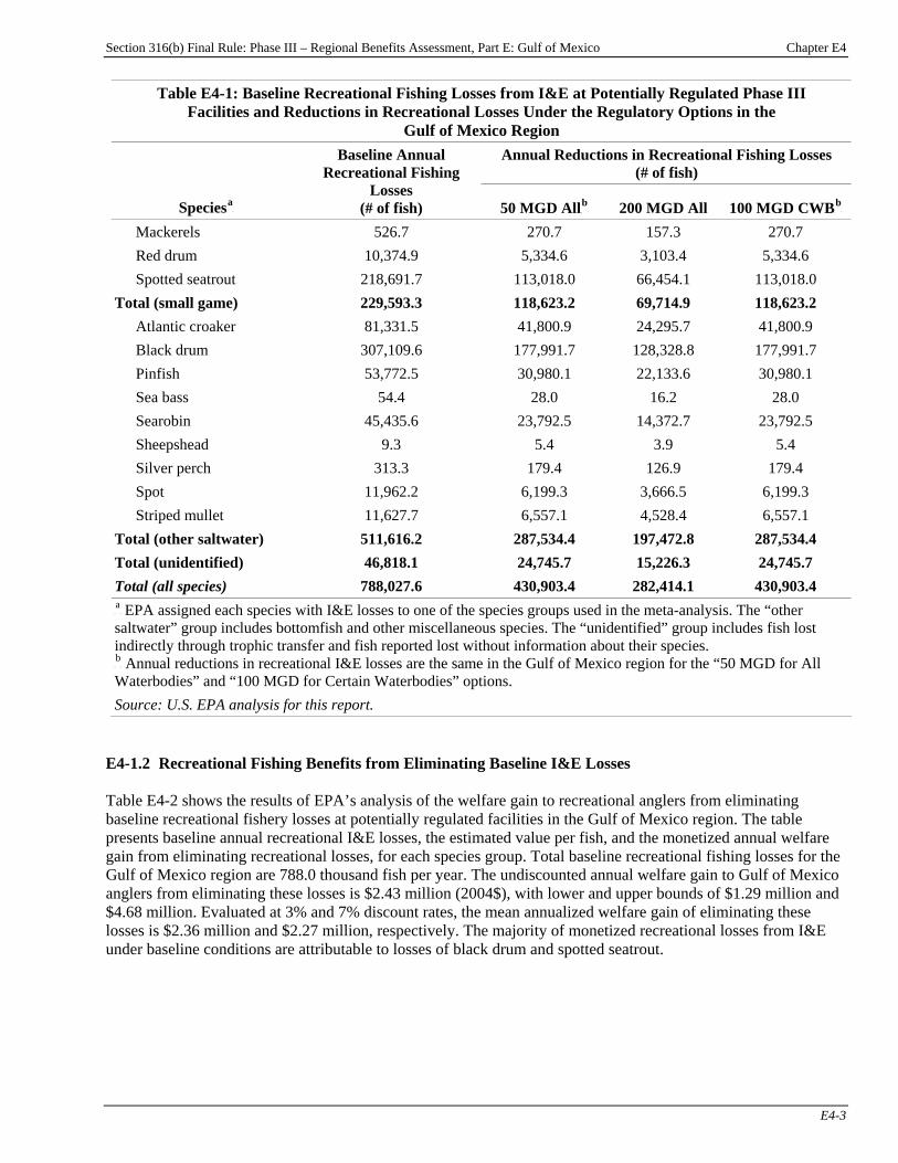
Section 316(b) Final Rule: Phase III – Regional Benefits Assessment, Part E: Gulf of Mexico Chapter E4
E4-3
Table E4-1: Baseline Recreational Fishing Losses from I&E at Potentially Regulated Phase III Facilities and Reductions in Recreational Losses Under the Regulatory Options in the
Gulf of Mexico Region Annual Reductions in Recreational Fishing Losses
(# of fish)
SpeciesP
aP
Baseline Annual Recreational Fishing
Losses (# of fish) 50 MGD AllP
bP 200 MGD All 100 MGD CWBP
bP
Mackerels 526.7 270.7 157.3 270.7 Red drum 10,374.9 5,334.6 3,103.4 5,334.6 Spotted seatrout 218,691.7 113,018.0 66,454.1 113,018.0
Total (small game) 229,593.3 118,623.2 69,714.9 118,623.2 Atlantic croaker 81,331.5 41,800.9 24,295.7 41,800.9 Black drum 307,109.6 177,991.7 128,328.8 177,991.7 Pinfish 53,772.5 30,980.1 22,133.6 30,980.1 Sea bass 54.4 28.0 16.2 28.0 Searobin 45,435.6 23,792.5 14,372.7 23,792.5 Sheepshead 9.3 5.4 3.9 5.4 Silver perch 313.3 179.4 126.9 179.4 Spot 11,962.2 6,199.3 3,666.5 6,199.3 Striped mullet 11,627.7 6,557.1 4,528.4 6,557.1
Total (other saltwater) 511,616.2 287,534.4 197,472.8 287,534.4 Total (unidentified) 46,818.1 24,745.7 15,226.3 24,745.7 Total (all species) 788,027.6 430,903.4 282,414.1 430,903.4 P
aP EPA assigned each species with I&E losses to one of the species groups used in the meta-analysis. The “other
saltwater” group includes bottomfish and other miscellaneous species. The “unidentified” group includes fish lost indirectly through trophic transfer and fish reported lost without information about their species. P
bP Annual reductions in recreational I&E losses are the same in the Gulf of Mexico region for the “50 MGD for All
Waterbodies” and “100 MGD for Certain Waterbodies” options. Source: U.S. EPA analysis for this report.
E4-1.2 Recreational Fishing Benefits from Eliminating Baseline I&E Losses Table E4-2 shows the results of EPA’s analysis of the welfare gain to recreational anglers from eliminating baseline recreational fishery losses at potentially regulated facilities in the Gulf of Mexico region. The table presents baseline annual recreational I&E losses, the estimated value per fish, and the monetized annual welfare gain from eliminating recreational losses, for each species group. Total baseline recreational fishing losses for the Gulf of Mexico region are 788.0 thousand fish per year. The undiscounted annual welfare gain to Gulf of Mexico anglers from eliminating these losses is $2.43 million (2004$), with lower and upper bounds of $1.29 million and $4.68 million. Evaluated at 3% and 7% discount rates, the mean annualized welfare gain of eliminating these losses is $2.36 million and $2.27 million, respectively. The majority of monetized recreational losses from I&E under baseline conditions are attributable to losses of black drum and spotted seatrout.
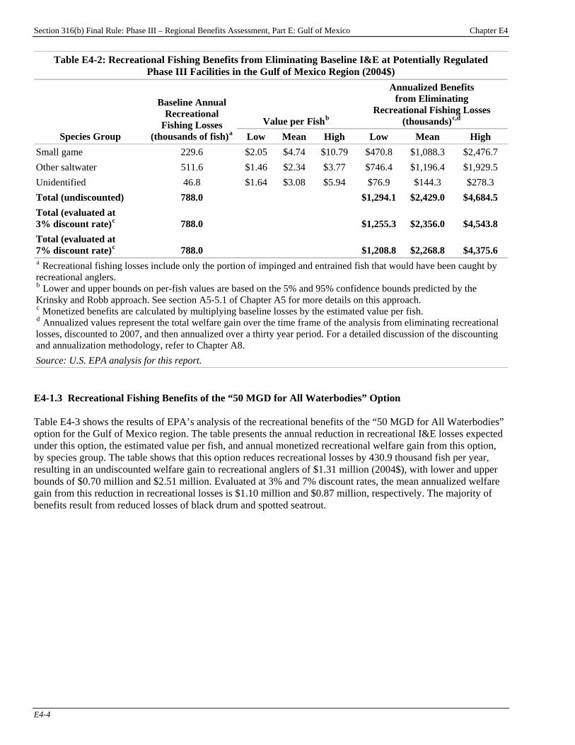
Section 316(b) Final Rule: Phase III – Regional Benefits Assessment, Part E: Gulf of Mexico Chapter E4
E4-4
Table E4-2: Recreational Fishing Benefits from Eliminating Baseline I&E at Potentially Regulated Phase III Facilities in the Gulf of Mexico Region (2004$)
Value per FishP
bP
Annualized Benefits from Eliminating
Recreational Fishing Losses (thousands)P
c,dP
Species Group
Baseline Annual Recreational
Fishing Losses (thousands of fish)P
aP Low Mean High Low Mean High
Small game 229.6 $2.05 $4.74 $10.79 $470.8 $1,088.3 $2,476.7 Other saltwater 511.6 $1.46 $2.34 $3.77 $746.4 $1,196.4 $1,929.5 Unidentified 46.8 $1.64 $3.08 $5.94 $76.9 $144.3 $278.3 Total (undiscounted) 788.0 $1,294.1 $2,429.0 $4,684.5 Total (evaluated at 3% discount rate)P
cP 788.0 $1,255.3 $2,356.0 $4,543.8
Total (evaluated at 7% discount rate)P
cP 788.0 $1,208.8 $2,268.8 $4,375.6
P
aP Recreational fishing losses include only the portion of impinged and entrained fish that would have been caught by
recreational anglers. P
bP Lower and upper bounds on per-fish values are based on the 5% and 95% confidence bounds predicted by the
Krinsky and Robb approach. See section A5-5.1 of Chapter A5 for more details on this approach. P
cP Monetized benefits are calculated by multiplying baseline losses by the estimated value per fish.
P
dP Annualized values represent the total welfare gain over the time frame of the analysis from eliminating recreational
losses, discounted to 2007, and then annualized over a thirty year period. For a detailed discussion of the discounting and annualization methodology, refer to Chapter A8. Source: U.S. EPA analysis for this report. E4-1.3 Recreational Fishing Benefits of the “50 MGD for All Waterbodies” Option Table E4-3 shows the results of EPA’s analysis of the recreational benefits of the “50 MGD for All Waterbodies” option for the Gulf of Mexico region. The table presents the annual reduction in recreational I&E losses expected under this option, the estimated value per fish, and annual monetized recreational welfare gain from this option, by species group. The table shows that this option reduces recreational losses by 430.9 thousand fish per year, resulting in an undiscounted welfare gain to recreational anglers of $1.31 million (2004$), with lower and upper bounds of $0.70 million and $2.51 million. Evaluated at 3% and 7% discount rates, the mean annualized welfare gain from this reduction in recreational losses is $1.10 million and $0.87 million, respectively. The majority of benefits result from reduced losses of black drum and spotted seatrout.
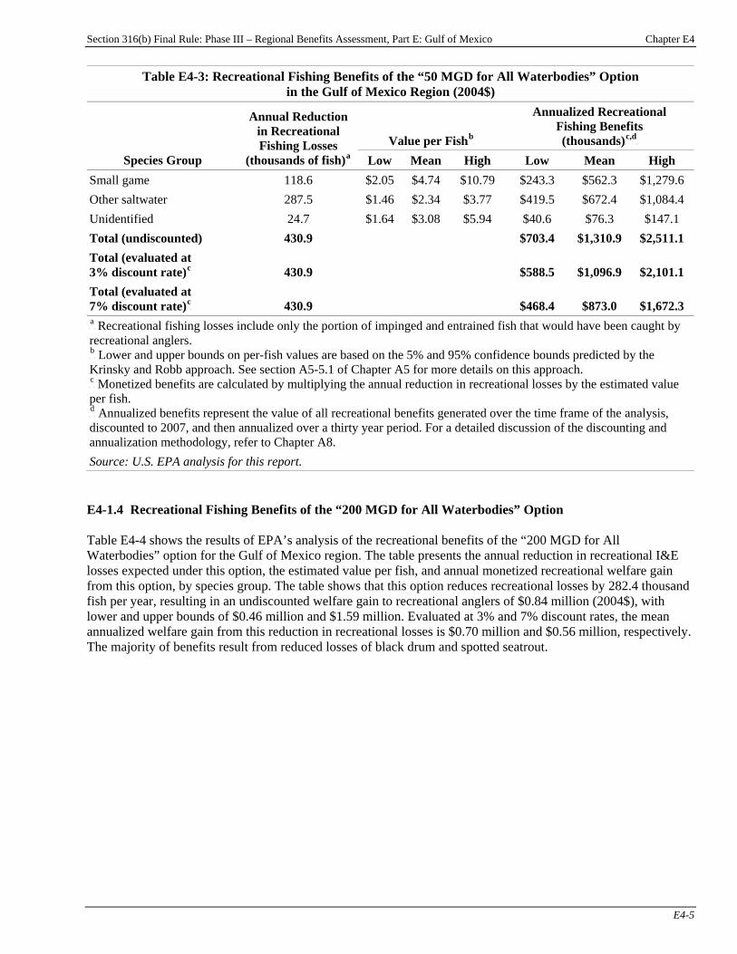
Section 316(b) Final Rule: Phase III – Regional Benefits Assessment, Part E: Gulf of Mexico Chapter E4
E4-5
Table E4-3: Recreational Fishing Benefits of the “50 MGD for All Waterbodies” Option in the Gulf of Mexico Region (2004$)
Value per FishP
bP
Annualized Recreational Fishing Benefits (thousands)P
c,dP
Species Group
Annual Reduction in Recreational Fishing Losses
(thousands of fish)P
aP Low Mean High Low Mean High
Small game 118.6 $2.05 $4.74 $10.79 $243.3 $562.3 $1,279.6 Other saltwater 287.5 $1.46 $2.34 $3.77 $419.5 $672.4 $1,084.4 Unidentified 24.7 $1.64 $3.08 $5.94 $40.6 $76.3 $147.1 Total (undiscounted) 430.9 $703.4 $1,310.9 $2,511.1 Total (evaluated at 3% discount rate)P
cP 430.9 $588.5 $1,096.9 $2,101.1
Total (evaluated at 7% discount rate)P
cP 430.9 $468.4 $873.0 $1,672.3
P
aP Recreational fishing losses include only the portion of impinged and entrained fish that would have been caught by
recreational anglers. P
bP Lower and upper bounds on per-fish values are based on the 5% and 95% confidence bounds predicted by the
Krinsky and Robb approach. See section A5-5.1 of Chapter A5 for more details on this approach. P
cP Monetized benefits are calculated by multiplying the annual reduction in recreational losses by the estimated value
per fish. P
dP Annualized benefits represent the value of all recreational benefits generated over the time frame of the analysis,
discounted to 2007, and then annualized over a thirty year period. For a detailed discussion of the discounting and annualization methodology, refer to Chapter A8. Source: U.S. EPA analysis for this report. E4-1.4 Recreational Fishing Benefits of the “200 MGD for All Waterbodies” Option Table E4-4 shows the results of EPA’s analysis of the recreational benefits of the “200 MGD for All Waterbodies” option for the Gulf of Mexico region. The table presents the annual reduction in recreational I&E losses expected under this option, the estimated value per fish, and annual monetized recreational welfare gain from this option, by species group. The table shows that this option reduces recreational losses by 282.4 thousand fish per year, resulting in an undiscounted welfare gain to recreational anglers of $0.84 million (2004$), with lower and upper bounds of $0.46 million and $1.59 million. Evaluated at 3% and 7% discount rates, the mean annualized welfare gain from this reduction in recreational losses is $0.70 million and $0.56 million, respectively. The majority of benefits result from reduced losses of black drum and spotted seatrout.
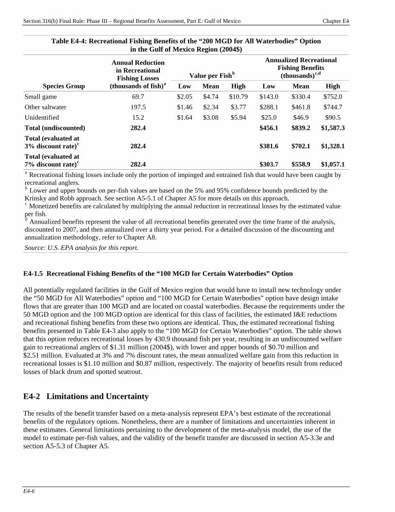
Section 316(b) Final Rule: Phase III – Regional Benefits Assessment, Part E: Gulf of Mexico Chapter E4
E4-6
Table E4-4: Recreational Fishing Benefits of the “200 MGD for All Waterbodies” Option in the Gulf of Mexico Region (2004$)
Value per FishP
bP
Annualized Recreational Fishing Benefits (thousands)P
c,dP
Species Group
Annual Reduction in Recreational Fishing Losses
(thousands of fish)P
aP Low Mean High Low Mean High
Small game 69.7 $2.05 $4.74 $10.79 $143.0 $330.4 $752.0 Other saltwater 197.5 $1.46 $2.34 $3.77 $288.1 $461.8 $744.7 Unidentified 15.2 $1.64 $3.08 $5.94 $25.0 $46.9 $90.5 Total (undiscounted) 282.4 $456.1 $839.2 $1,587.3 Total (evaluated at 3% discount rate)P
cP 282.4 $381.6 $702.1 $1,328.1
Total (evaluated at 7% discount rate)P
cP 282.4 $303.7 $558.9 $1,057.1
P
aP Recreational fishing losses include only the portion of impinged and entrained fish that would have been caught by
recreational anglers. P
bP Lower and upper bounds on per-fish values are based on the 5% and 95% confidence bounds predicted by the
Krinsky and Robb approach. See section A5-5.1 of Chapter A5 for more details on this approach. P
cP Monetized benefits are calculated by multiplying the annual reduction in recreational losses by the estimated value
per fish. P
dP Annualized benefits represent the value of all recreational benefits generated over the time frame of the analysis,
discounted to 2007, and then annualized over a thirty year period. For a detailed discussion of the discounting and annualization methodology, refer to Chapter A8. Source: U.S. EPA analysis for this report. E4-1.5 Recreational Fishing Benefits of the “100 MGD for Certain Waterbodies” Option All potentially regulated facilities in the Gulf of Mexico region that would have to install new technology under the “50 MGD for All Waterbodies” option and “100 MGD for Certain Waterbodies” option have design intake flows that are greater than 100 MGD and are located on coastal waterbodies. Because the requirements under the 50 MGD option and the 100 MGD option are identical for this class of facilities, the estimated I&E reductions and recreational fishing benefits from these two options are identical. Thus, the estimated recreational fishing benefits presented in Table E4-3 also apply to the “100 MGD for Certain Waterbodies” option. The table shows that this option reduces recreational losses by 430.9 thousand fish per year, resulting in an undiscounted welfare gain to recreational anglers of $1.31 million (2004$), with lower and upper bounds of $0.70 million and $2.51 million. Evaluated at 3% and 7% discount rates, the mean annualized welfare gain from this reduction in recreational losses is $1.10 million and $0.87 million, respectively. The majority of benefits result from reduced losses of black drum and spotted seatrout. E4-2 Limitations and Uncertainty The results of the benefit transfer based on a meta-analysis represent EPA’s best estimate of the recreational benefits of the regulatory options. Nonetheless, there are a number of limitations and uncertainties inherent in these estimates. General limitations pertaining to the development of the meta-analysis model, the use of the model to estimate per-fish values, and the validity of the benefit transfer are discussed in section A5-3.3e and section A5-5.3 of Chapter A5.
Section 316(b) Final Rule: Phase III – Regional Benefits Assessment, Part E: Gulf of Mexico Appendix E4
App. E4-1
Appendix E4: Recreational Use Benefits Under Supplemental Policy Options
Introduction
Appendix Contents E4-1 Recreational Fishing Benefits of the Supplemental Options ..................................E4-1 E4-1.1 Estimated Reductions in Recreational Fishing Losses Under the Supplemental Options....E4-1 E4-1.2 Recreational Fishing Benefits of the Supplemental Options ..............E4-3 E4-2 Comparison of Recreational Fishing
Benefits by Option .......................................E4-6
Chapter E4 presents EPA’s estimates of the recreational benefits of the regulatory options for the section 316(b) rule for Phase III facilities in the Gulf of Mexico region. To facilitate comparisons among the options, this appendix presents estimates of the recreational fishing benefits of several supplemental options that EPA evaluated in preparation for this rule:
< “Electric Generators 2-50 MGD I-only Everywhere” option,
< “Electric Generators 2-50 MGD I&E like Phase II” option; < “Electric Generators 2-50 MGD I&E Everywhere” option; < “Manufacturers 2-50 MGD I-only Everywhere” option; < “Manufacturers 2-50 MGD I&E like Phase II” option; < “Manufacturers 2-50 MGD I&E Everywhere” option; < “Manufacturers 50+ MGD I-only Everywhere” option; and < “Manufacturers 50+ MGD I&E Everywhere” option.
Recreational fishing benefits presented in this chapter were estimated using the benefit transfer approach discussed in Chapter E4 and in Chapter A5, “Recreational Fishing Benefits Methodology.” E4-1 Recreational Fishing Benefits of the Supplemental Options E4-1.1 Estimated Reductions in Recreational Fishing Losses Under the Supplemental Options Table E4-1 presents EPA’s estimates of the annual reduction in baseline (i.e., current) recreational fishing losses from impingement and entrainment (I&E) in the Gulf of Mexico region under the supplemental options. For more information on the options, please see the TDD.

Section 316(b) Final Rule: Phase III – Regional Benefits Assessment, Part E: Gulf of Mexico Appendix E4
App. E4-2
Table E4-1: Reductions in Recreational Fishing Losses from I&E Under the Supplemental Options in the Gulf of Mexico Region Annual Reduction in Recreational Losses
(# of fish) Electric Generators 2-50 MGDP
bP Manufacturers 2-50 MGD Manufacturers 50+ MGD
SpeciesP
aP
I-only Everywhere
I&E like Phase II
I&E Everywhere
I-only Everywhere
I&E like Phase IIP
cP
I&E EverywhereP
cP
I-only Everywhere
I&E Everywhere
Mackerels 0 0 0 14.1 14.1 14.1 270.7 270.7 Red drum 0 0 0 277.0 277.8 277.8 5,311.5 5,334.6 Spotted seatrout 0 0 0 5,606.5 5,797.3 5,797.3 107,512.2 113,018.0
Total (small game) 0 0 0 5,897.6 6,089.2 6,089.2 113,094.4 118,623.2 Atlantic croaker 0 0 0 2,178.7 2,179.4 2,179.4 41,779.6 41,800.9 Black drum 0 0 0 41.1 6,183.2 6,183.2 787.7 177,991.7 Pinfish 0 0 0 82.3 1,101.4 1,101.4 1,578.4 30,980.1 Sea bass 0 0 0 1.5 1.5 1.5 28.0 28.0 Searobin 0 0 0 1,038.2 1,172.8 1,172.8 19,907.9 23,792.5 Sheepshead 0 0 0 0.0 0.2 0.2 0.1 5.4 Silver perch 0 0 0 0.9 6.5 6.5 18.0 179.4 Spot 0 0 0 299.6 315.3 315.3 5,745.3 6,199.3 Striped mullet 0 0 0 75.5 252.6 252.6 1,447.2 6,557.1
Total (other saltwater) 0 0 0 3,717.7 11,212.9 11,212.9 71,292.2 287,534.4 Total (unidentified) 0 0 0 976.6 1,185.2 1,185.2 18,727.7 24,745.7 Total (all species) 0 0 0 10,591.9 18,487.4 18,487.4 203,114.3 430,903.4 P
aP EPA assigned each species with I&E losses to one of the species groups used in the meta-analysis. The “other saltwater” group includes bottomfish and other
miscellaneous species. The “unidentified” group includes fish lost indirectly through trophic transfer and fish reported lost without information about their species.P
bP No facilities located in the Gulf of Mexico region are electric generators with design intake flows greater than 2 MGD and less than 50 MGD. Thus no facilities
would have technology requirements under the “Electric Generators 2-50 MGD I-only Everywhere” option, the “Electric Generators 2-50 MGD I&E like Phase II” option, or the “Electric Generators 2-50 MGD I&E Everywhere” option. P
cP Annual reductions in recreational I&E losses are the same in the Gulf of Mexico region for the “Manufacturers 2-50 MGD I&E like Phase II” and
“Manufacturers 2-50 MGD I&E Everywhere” options. Source: U.S. EPA analysis for this report.
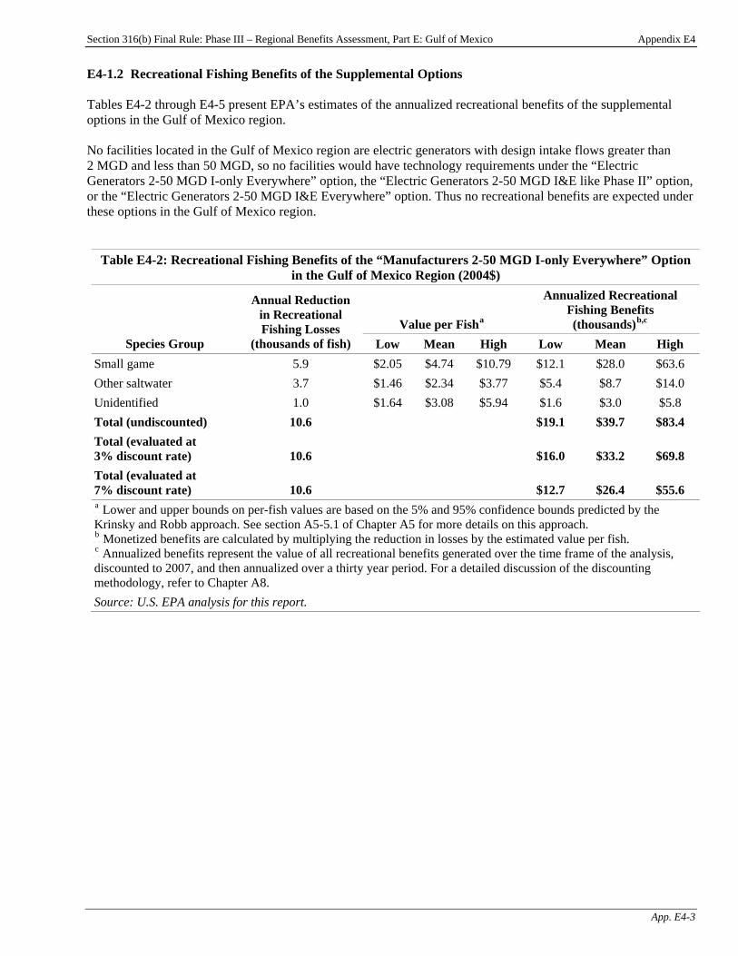
Section 316(b) Final Rule: Phase III – Regional Benefits Assessment, Part E: Gulf of Mexico Appendix E4
App. E4-3
E4-1.2 Recreational Fishing Benefits of the Supplemental Options Tables E4-2 through E4-5 present EPA’s estimates of the annualized recreational benefits of the supplemental options in the Gulf of Mexico region. No facilities located in the Gulf of Mexico region are electric generators with design intake flows greater than 2 MGD and less than 50 MGD, so no facilities would have technology requirements under the “Electric Generators 2-50 MGD I-only Everywhere” option, the “Electric Generators 2-50 MGD I&E like Phase II” option, or the “Electric Generators 2-50 MGD I&E Everywhere” option. Thus no recreational benefits are expected under these options in the Gulf of Mexico region.
Table E4-2: Recreational Fishing Benefits of the “Manufacturers 2-50 MGD I-only Everywhere” Option in the Gulf of Mexico Region (2004$)
Value per FishP
aP
Annualized Recreational Fishing Benefits (thousands)P
b,cP
Species Group
Annual Reduction in Recreational Fishing Losses
(thousands of fish) Low Mean High Low Mean High Small game 5.9 $2.05 $4.74 $10.79 $12.1 $28.0 $63.6 Other saltwater 3.7 $1.46 $2.34 $3.77 $5.4 $8.7 $14.0 Unidentified 1.0 $1.64 $3.08 $5.94 $1.6 $3.0 $5.8 Total (undiscounted) 10.6 $19.1 $39.7 $83.4 Total (evaluated at 3% discount rate) 10.6 $16.0 $33.2 $69.8 Total (evaluated at 7% discount rate) 10.6 $12.7 $26.4 $55.6 P
aP Lower and upper bounds on per-fish values are based on the 5% and 95% confidence bounds predicted by the
Krinsky and Robb approach. See section A5-5.1 of Chapter A5 for more details on this approach. P
bP Monetized benefits are calculated by multiplying the reduction in losses by the estimated value per fish.
P
cP Annualized benefits represent the value of all recreational benefits generated over the time frame of the analysis,
discounted to 2007, and then annualized over a thirty year period. For a detailed discussion of the discounting methodology, refer to Chapter A8. Source: U.S. EPA analysis for this report.
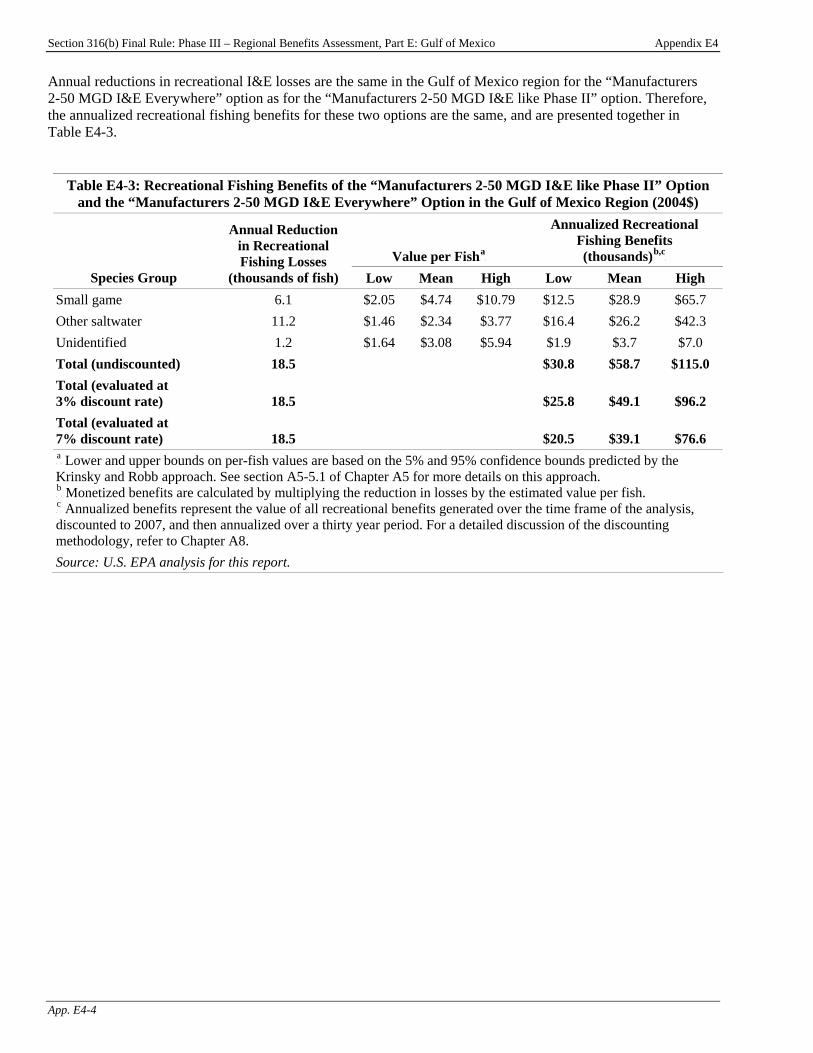
Section 316(b) Final Rule: Phase III – Regional Benefits Assessment, Part E: Gulf of Mexico Appendix E4
App. E4-4
Annual reductions in recreational I&E losses are the same in the Gulf of Mexico region for the “Manufacturers 2-50 MGD I&E Everywhere” option as for the “Manufacturers 2-50 MGD I&E like Phase II” option. Therefore, the annualized recreational fishing benefits for these two options are the same, and are presented together in Table E4-3.
Table E4-3: Recreational Fishing Benefits of the “Manufacturers 2-50 MGD I&E like Phase II” Option and the “Manufacturers 2-50 MGD I&E Everywhere” Option in the Gulf of Mexico Region (2004$)
Value per FishP
aP
Annualized Recreational Fishing Benefits (thousands)P
b,cP
Species Group
Annual Reduction in Recreational Fishing Losses
(thousands of fish) Low Mean High Low Mean High Small game 6.1 $2.05 $4.74 $10.79 $12.5 $28.9 $65.7 Other saltwater 11.2 $1.46 $2.34 $3.77 $16.4 $26.2 $42.3 Unidentified 1.2 $1.64 $3.08 $5.94 $1.9 $3.7 $7.0 Total (undiscounted) 18.5 $30.8 $58.7 $115.0 Total (evaluated at 3% discount rate) 18.5 $25.8 $49.1 $96.2 Total (evaluated at 7% discount rate) 18.5 $20.5 $39.1 $76.6 P
aP Lower and upper bounds on per-fish values are based on the 5% and 95% confidence bounds predicted by the
Krinsky and Robb approach. See section A5-5.1 of Chapter A5 for more details on this approach. P
bP Monetized benefits are calculated by multiplying the reduction in losses by the estimated value per fish.
P
cP Annualized benefits represent the value of all recreational benefits generated over the time frame of the analysis,
discounted to 2007, and then annualized over a thirty year period. For a detailed discussion of the discounting methodology, refer to Chapter A8. Source: U.S. EPA analysis for this report.
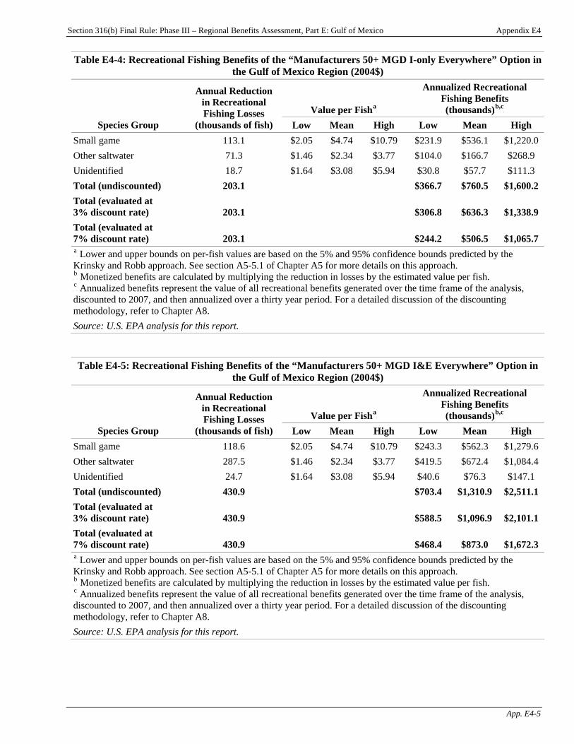
Section 316(b) Final Rule: Phase III – Regional Benefits Assessment, Part E: Gulf of Mexico Appendix E4
App. E4-5
Table E4-4: Recreational Fishing Benefits of the “Manufacturers 50+ MGD I-only Everywhere” Option in the Gulf of Mexico Region (2004$)
Value per FishP
aP
Annualized Recreational Fishing Benefits (thousands)P
b,cP
Species Group
Annual Reduction in Recreational Fishing Losses
(thousands of fish) Low Mean High Low Mean High Small game 113.1 $2.05 $4.74 $10.79 $231.9 $536.1 $1,220.0 Other saltwater 71.3 $1.46 $2.34 $3.77 $104.0 $166.7 $268.9 Unidentified 18.7 $1.64 $3.08 $5.94 $30.8 $57.7 $111.3 Total (undiscounted) 203.1 $366.7 $760.5 $1,600.2 Total (evaluated at 3% discount rate) 203.1 $306.8 $636.3 $1,338.9 Total (evaluated at 7% discount rate) 203.1 $244.2 $506.5 $1,065.7 P
aP Lower and upper bounds on per-fish values are based on the 5% and 95% confidence bounds predicted by the
Krinsky and Robb approach. See section A5-5.1 of Chapter A5 for more details on this approach. P
bP Monetized benefits are calculated by multiplying the reduction in losses by the estimated value per fish.
P
cP Annualized benefits represent the value of all recreational benefits generated over the time frame of the analysis,
discounted to 2007, and then annualized over a thirty year period. For a detailed discussion of the discounting methodology, refer to Chapter A8. Source: U.S. EPA analysis for this report.
Table E4-5: Recreational Fishing Benefits of the “Manufacturers 50+ MGD I&E Everywhere” Option in the Gulf of Mexico Region (2004$)
Value per FishP
aP
Annualized Recreational Fishing Benefits (thousands)P
b,cP
Species Group
Annual Reduction in Recreational Fishing Losses
(thousands of fish) Low Mean High Low Mean High Small game 118.6 $2.05 $4.74 $10.79 $243.3 $562.3 $1,279.6 Other saltwater 287.5 $1.46 $2.34 $3.77 $419.5 $672.4 $1,084.4 Unidentified 24.7 $1.64 $3.08 $5.94 $40.6 $76.3 $147.1 Total (undiscounted) 430.9 $703.4 $1,310.9 $2,511.1 Total (evaluated at 3% discount rate) 430.9 $588.5 $1,096.9 $2,101.1 Total (evaluated at 7% discount rate) 430.9 $468.4 $873.0 $1,672.3 P
aP Lower and upper bounds on per-fish values are based on the 5% and 95% confidence bounds predicted by the
Krinsky and Robb approach. See section A5-5.1 of Chapter A5 for more details on this approach. P
bP Monetized benefits are calculated by multiplying the reduction in losses by the estimated value per fish.
P
cP Annualized benefits represent the value of all recreational benefits generated over the time frame of the analysis,
discounted to 2007, and then annualized over a thirty year period. For a detailed discussion of the discounting methodology, refer to Chapter A8. Source: U.S. EPA analysis for this report.
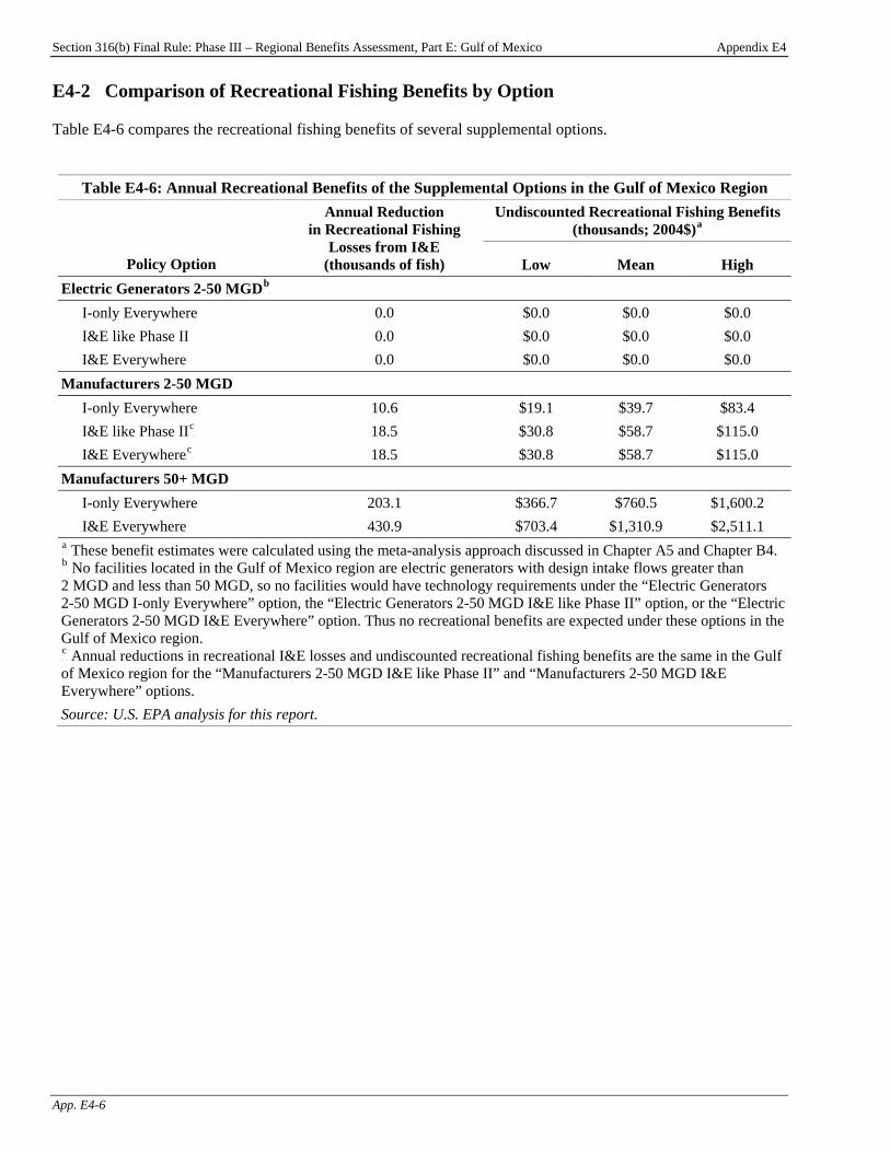
Section 316(b) Final Rule: Phase III – Regional Benefits Assessment, Part E: Gulf of Mexico Appendix E4
App. E4-6
E4-2 Comparison of Recreational Fishing Benefits by Option Table E4-6 compares the recreational fishing benefits of several supplemental options.
Table E4-6: Annual Recreational Benefits of the Supplemental Options in the Gulf of Mexico Region Undiscounted Recreational Fishing Benefits
(thousands; 2004$)P
aP
Policy Option
Annual Reduction in Recreational Fishing
Losses from I&E (thousands of fish) Low Mean High
Electric Generators 2-50 MGDP
bP
I-only Everywhere 0.0 $0.0 $0.0 $0.0 I&E like Phase II 0.0 $0.0 $0.0 $0.0 I&E Everywhere 0.0 $0.0 $0.0 $0.0
Manufacturers 2-50 MGD I-only Everywhere 10.6 $19.1 $39.7 $83.4 I&E like Phase IIP
cP 18.5 $30.8 $58.7 $115.0
I&E EverywhereP
cP 18.5 $30.8 $58.7 $115.0
Manufacturers 50+ MGD I-only Everywhere 203.1 $366.7 $760.5 $1,600.2 I&E Everywhere 430.9 $703.4 $1,310.9 $2,511.1
P
aP These benefit estimates were calculated using the meta-analysis approach discussed in Chapter A5 and Chapter B4.
P
bP No facilities located in the Gulf of Mexico region are electric generators with design intake flows greater than
2 MGD and less than 50 MGD, so no facilities would have technology requirements under the “Electric Generators 2-50 MGD I-only Everywhere” option, the “Electric Generators 2-50 MGD I&E like Phase II” option, or the “Electric Generators 2-50 MGD I&E Everywhere” option. Thus no recreational benefits are expected under these options in the Gulf of Mexico region. P
cP Annual reductions in recreational I&E losses and undiscounted recreational fishing benefits are the same in the Gulf
of Mexico region for the “Manufacturers 2-50 MGD I&E like Phase II” and “Manufacturers 2-50 MGD I&E Everywhere” options. Source: U.S. EPA analysis for this report.

Section 316(b) Final Rule: Phase III – Regional Benefits Assessment, Part E: Gulf of Mexico Chapter E5
E5-1
Chapter E5: Federally Listed T&E Species in the Gulf of Mexico Region
This chapter lists current federally listed threatened and endangered (T&E) fish and shellfish species in the Gulf of Mexico Region. This list does not address proposed or candidate species; In addition, fish and shellfish listed as cave species, marine mammals, reptiles, amphibians, and snails are not included in this chapter.
Table E5-1: Alabama Federally Listed T&E Fish and Shellfish Status Scientific Name Common Name
T Acipenser oxyrinchus desotoi Gulf sturgeon E Dromus dromas Dromedary pearlymussel: entire range except where
listed as experimental populations T Elliptoideus sloatianus Purple bankclimber mussel E Epioblasma florentina walkeri ( = E. walkeri) Tan riffleshell mussel E Epioblasma othcaloogensis Southern acornshell mussel E Epioblasma torulosa torulosa Tubercled blossom pearlymussel: entire range except
where listed as experimental populations E Leptodea leptodon Scaleshell mussel E Medionidus parvulus Moccasinshell mussel E Medionidus penicillatus Gulf moccasinshell mussel E Pegias fabula Littlewing pearlymussel E Percina antesella Amber darter E Pleurobema clava Clubshell mussel: entire range except where listed as
experimental populations E Pleurobema curtum Black clubshell mussel E Pleurobema pyriforme Oval pigtoe mussel E Pristis pectinata Smalltooth sawfish E Quadrula fragosa Winged mapleleaf mussel: entire range except where
listed as experimental populations E Villosa trabalis Cumberland bean pearlymussel: entire range except
where listed as experimental populations Source: USFWS, 2006a.
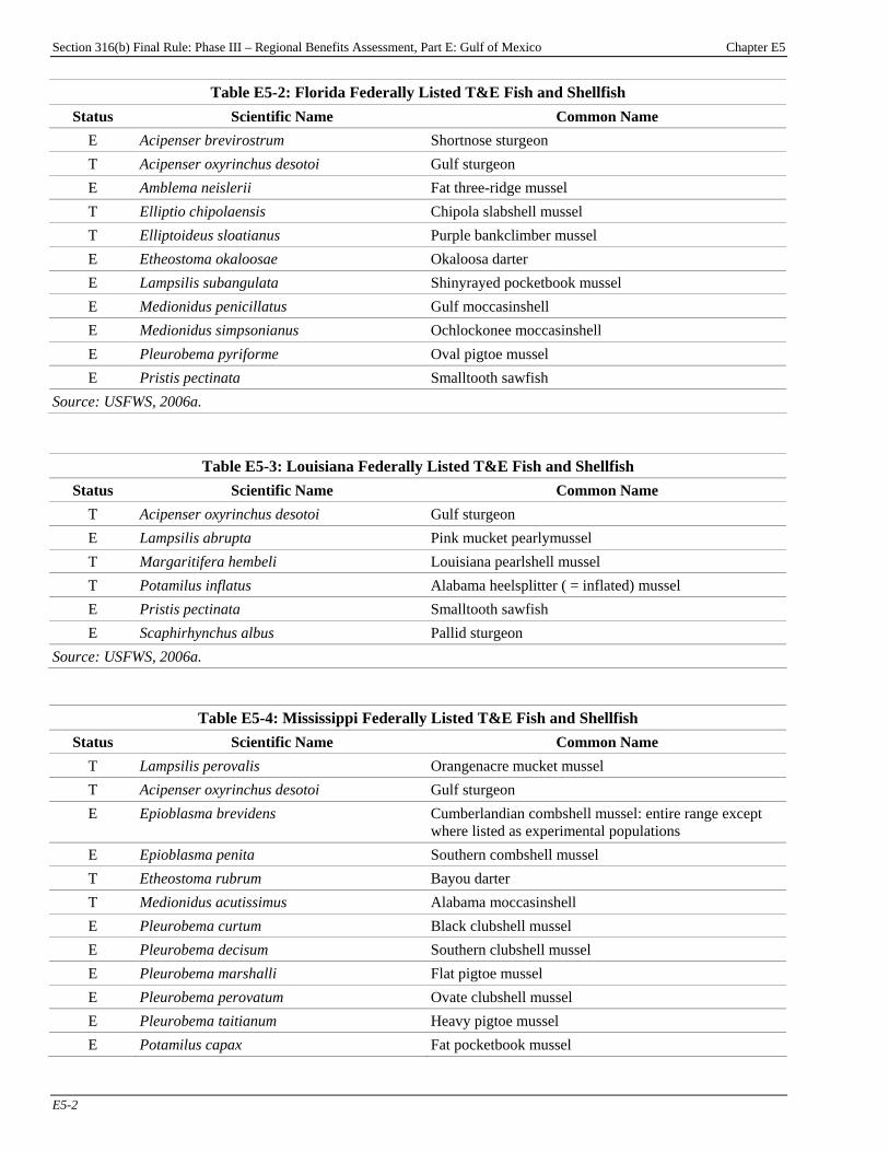
Section 316(b) Final Rule: Phase III – Regional Benefits Assessment, Part E: Gulf of Mexico Chapter E5
E5-2
Table E5-2: Florida Federally Listed T&E Fish and Shellfish Status Scientific Name Common Name
E Acipenser brevirostrum Shortnose sturgeon T Acipenser oxyrinchus desotoi Gulf sturgeon E Amblema neislerii Fat three-ridge mussel T Elliptio chipolaensis Chipola slabshell mussel T Elliptoideus sloatianus Purple bankclimber mussel E Etheostoma okaloosae Okaloosa darter E Lampsilis subangulata Shinyrayed pocketbook mussel E Medionidus penicillatus Gulf moccasinshell E Medionidus simpsonianus Ochlockonee moccasinshell E Pleurobema pyriforme Oval pigtoe mussel E Pristis pectinata Smalltooth sawfish
Source: USFWS, 2006a.
Table E5-3: Louisiana Federally Listed T&E Fish and Shellfish Status Scientific Name Common Name
T Acipenser oxyrinchus desotoi Gulf sturgeon E Lampsilis abrupta Pink mucket pearlymussel T Margaritifera hembeli Louisiana pearlshell mussel T Potamilus inflatus Alabama heelsplitter ( = inflated) mussel E Pristis pectinata Smalltooth sawfish E Scaphirhynchus albus Pallid sturgeon
Source: USFWS, 2006a.
Table E5-4: Mississippi Federally Listed T&E Fish and Shellfish Status Scientific Name Common Name
T Lampsilis perovalis Orangenacre mucket mussel T Acipenser oxyrinchus desotoi Gulf sturgeon E Epioblasma brevidens Cumberlandian combshell mussel: entire range except
where listed as experimental populations E Epioblasma penita Southern combshell mussel T Etheostoma rubrum Bayou darter T Medionidus acutissimus Alabama moccasinshell E Pleurobema curtum Black clubshell mussel E Pleurobema decisum Southern clubshell mussel E Pleurobema marshalli Flat pigtoe mussel E Pleurobema perovatum Ovate clubshell mussel E Pleurobema taitianum Heavy pigtoe mussel E Potamilus capax Fat pocketbook mussel

Section 316(b) Final Rule: Phase III – Regional Benefits Assessment, Part E: Gulf of Mexico Chapter E5
E5-3
Table E5-4: Mississippi Federally Listed T&E Fish and Shellfish Status Scientific Name Common Name
T Potamilus inflatus Alabama heelsplitter ( = inflated) mussel E Pristis pectinata Smalltooth sawfish E Quadrula stapes Stirrupshell mussel E Scaphirhynchus albus Pallid sturgeon E Scaphirhynchus suttkusi Alabama sturgeon
Source: USFWS, 2006a.
Table E5-5: Texas Federally Listed T&E Fish and Shellfish Status Scientific Name Common Name
E Cyprinodon bovinus Leon Springs pupfish E Cyprinodon elegans Comanche Springs pupfish T Dionda diaboli Devils River minnow E Etheostoma fonticola Fountain darter E Gambusia gaigei Big Bend gambusia E Gambusia georgei San Marcos gambusia E Gambusia heterochir Clear Creek gambusia E Gambusia nobilis Pecos gambusia E Hybognathus amarus Rio Grande silvery minnow T Notropis girardi Arkansas River shiner (Arkansas River basin) E Pristis pectinata Smalltooth sawfish
Source: USFWS, 2006a.

Section 316(b) Final Rule: Phase III – Regional Benefits Assessment
Part F: The Great Lakes
Section 316(b) Final Rule: Phase III – Regional Benefits Assessment, Part F: The Great Lakes Chapter F1
F1-1
Chapter F1: Background Introduction This chapter presents an overview of the potential Phase III existing facilities in the Great Lakes study region and summarizes their key cooling water and compliance characteristics. For further discussion of the technical and compliance characteristics of potential Phase III existing facilities, refer to the Economic Analysis for the Final Section 316(b) Rule for Phase III Facilities and the Technical Development Document for the Final Section 316(b) Rule for Phase III Facilities (U.S. EPA, 2006a,c).
Chapter Contents F1-1 Facility Characteristics.................................. F1-1
F1-1 Facility Characteristics The Great Lakes Regional Study includes 17 sample facilities that are potentially subject to the national standards for Phase III existing facilities. Figure F1-1 presents a map of these facilities. Thirteen of them are manufacturing facilities and four are electric generators. Industry-wide, these 17 sample facilities represent 43 facilities.PF
1FP
P
1P EPA applied sample weights to the survey respondents to account for non-sampled facilities and facilities that did
not respond to the survey. For more information on EPA’s 2000 Section 316(b) Industry Survey, please refer to the Information Collection Request (U.S. EPA, 2000b).

Section 316(b) Final Rule: Phase III – Regional Benefits Assessment, Part F: The Great Lakes Chapter F1
F1-2
Figure F1-1: Potential Existing Phase III Facilities in the Great Lakes Regional StudyP
aP
P
aP The map includes locations of sample facilities only.
Source: U.S. EPA analysis for this report.
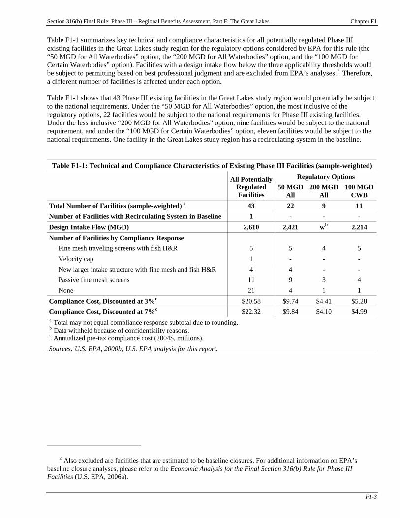
Section 316(b) Final Rule: Phase III – Regional Benefits Assessment, Part F: The Great Lakes Chapter F1
F1-3
Table F1-1 summarizes key technical and compliance characteristics for all potentially regulated Phase III existing facilities in the Great Lakes study region for the regulatory options considered by EPA for this rule (the “50 MGD for All Waterbodies” option, the “200 MGD for All Waterbodies” option, and the “100 MGD for Certain Waterbodies” option). Facilities with a design intake flow below the three applicability thresholds would be subject to permitting based on best professional judgment and are excluded from EPA’s analyses.PF
2FP Therefore,
a different number of facilities is affected under each option. Table F1-1 shows that 43 Phase III existing facilities in the Great Lakes study region would potentially be subject to the national requirements. Under the “50 MGD for All Waterbodies” option, the most inclusive of the regulatory options, 22 facilities would be subject to the national requirements for Phase III existing facilities. Under the less inclusive “200 MGD for All Waterbodies” option, nine facilities would be subject to the national requirement, and under the “100 MGD for Certain Waterbodies” option, eleven facilities would be subject to the national requirements. One facility in the Great Lakes study region has a recirculating system in the baseline.
Table F1-1: Technical and Compliance Characteristics of Existing Phase III Facilities (sample-weighted) Regulatory Options
All Potentially
Regulated Facilities
50 MGD All
200 MGD All
100 MGD CWB
Total Number of Facilities (sample-weighted)P
aP 43 22 9 11
Number of Facilities with Recirculating System in Baseline 1 - - - Design Intake Flow (MGD) 2,610 2,421 wP
bP 2,214
Number of Facilities by Compliance Response Fine mesh traveling screens with fish H&R 5 5 4 5 Velocity cap 1 - - - New larger intake structure with fine mesh and fish H&R 4 4 - - Passive fine mesh screens 11 9 3 4 None 21 4 1 1
Compliance Cost, Discounted at 3%P
cP $20.58 $9.74 $4.41 $5.28
Compliance Cost, Discounted at 7%P
cP $22.32 $9.84 $4.10 $4.99
P
aP Total may not equal compliance response subtotal due to rounding.
P
bP Data withheld because of confidentiality reasons.
P
cP Annualized pre-tax compliance cost (2004$, millions).
Sources: U.S. EPA, 2000b; U.S. EPA analysis for this report.
P
2P Also excluded are facilities that are estimated to be baseline closures. For additional information on EPA’s
baseline closure analyses, please refer to the Economic Analysis for the Final Section 316(b) Rule for Phase III Facilities (U.S. EPA, 2006a).
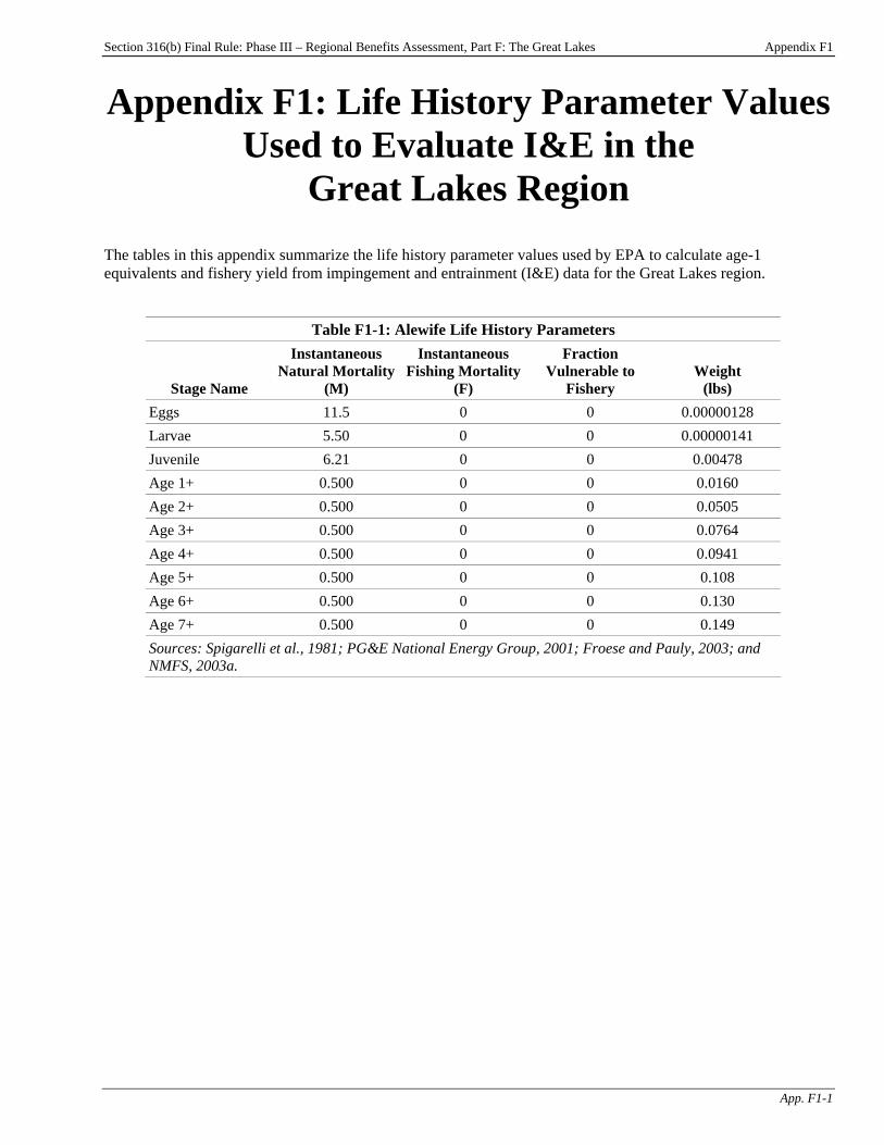
Section 316(b) Final Rule: Phase III – Regional Benefits Assessment, Part F: The Great Lakes Appendix F1
App. F1-1
Appendix F1: Life History Parameter Values Used to Evaluate I&E in the
Great Lakes Region The tables in this appendix summarize the life history parameter values used by EPA to calculate age-1 equivalents and fishery yield from impingement and entrainment (I&E) data for the Great Lakes region.
Table F1-1: Alewife Life History Parameters
Stage Name
Instantaneous Natural Mortality
(M)
Instantaneous Fishing Mortality
(F)
Fraction Vulnerable to
Fishery Weight
(lbs) Eggs 11.5 0 0 0.00000128 Larvae 5.50 0 0 0.00000141 Juvenile 6.21 0 0 0.00478 Age 1+ 0.500 0 0 0.0160 Age 2+ 0.500 0 0 0.0505 Age 3+ 0.500 0 0 0.0764 Age 4+ 0.500 0 0 0.0941 Age 5+ 0.500 0 0 0.108 Age 6+ 0.500 0 0 0.130 Age 7+ 0.500 0 0 0.149 Sources: Spigarelli et al., 1981; PG&E National Energy Group, 2001; Froese and Pauly, 2003; and NMFS, 2003a.
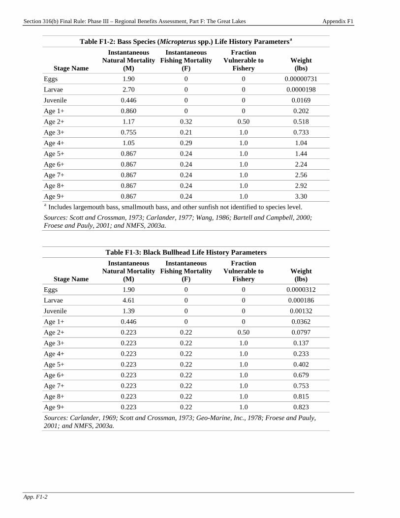
Section 316(b) Final Rule: Phase III – Regional Benefits Assessment, Part F: The Great Lakes Appendix F1
App. F1-2
Table F1-2: Bass Species (Micropterus spp.) Life History ParametersP
aP
Stage Name
Instantaneous Natural Mortality
(M)
Instantaneous Fishing Mortality
(F)
Fraction Vulnerable to
Fishery Weight
(lbs) Eggs 1.90 0 0 0.00000731 Larvae 2.70 0 0 0.0000198 Juvenile 0.446 0 0 0.0169 Age 1+ 0.860 0 0 0.202 Age 2+ 1.17 0.32 0.50 0.518 Age 3+ 0.755 0.21 1.0 0.733 Age 4+ 1.05 0.29 1.0 1.04 Age 5+ 0.867 0.24 1.0 1.44 Age 6+ 0.867 0.24 1.0 2.24 Age 7+ 0.867 0.24 1.0 2.56 Age 8+ 0.867 0.24 1.0 2.92 Age 9+ 0.867 0.24 1.0 3.30 P
aP Includes largemouth bass, smallmouth bass, and other sunfish not identified to species level.
Sources: Scott and Crossman, 1973; Carlander, 1977; Wang, 1986; Bartell and Campbell, 2000; Froese and Pauly, 2001; and NMFS, 2003a.
Table F1-3: Black Bullhead Life History Parameters
Stage Name
Instantaneous Natural Mortality
(M)
Instantaneous Fishing Mortality
(F)
Fraction Vulnerable to
Fishery Weight
(lbs) Eggs 1.90 0 0 0.0000312 Larvae 4.61 0 0 0.000186 Juvenile 1.39 0 0 0.00132 Age 1+ 0.446 0 0 0.0362 Age 2+ 0.223 0.22 0.50 0.0797 Age 3+ 0.223 0.22 1.0 0.137 Age 4+ 0.223 0.22 1.0 0.233 Age 5+ 0.223 0.22 1.0 0.402 Age 6+ 0.223 0.22 1.0 0.679 Age 7+ 0.223 0.22 1.0 0.753 Age 8+ 0.223 0.22 1.0 0.815 Age 9+ 0.223 0.22 1.0 0.823 TSources: Carlander, 1969; Scott and Crossman, 1973; Geo-Marine, Inc., 1978; Froese and Pauly, 2001;T and NMFS, 2003a.
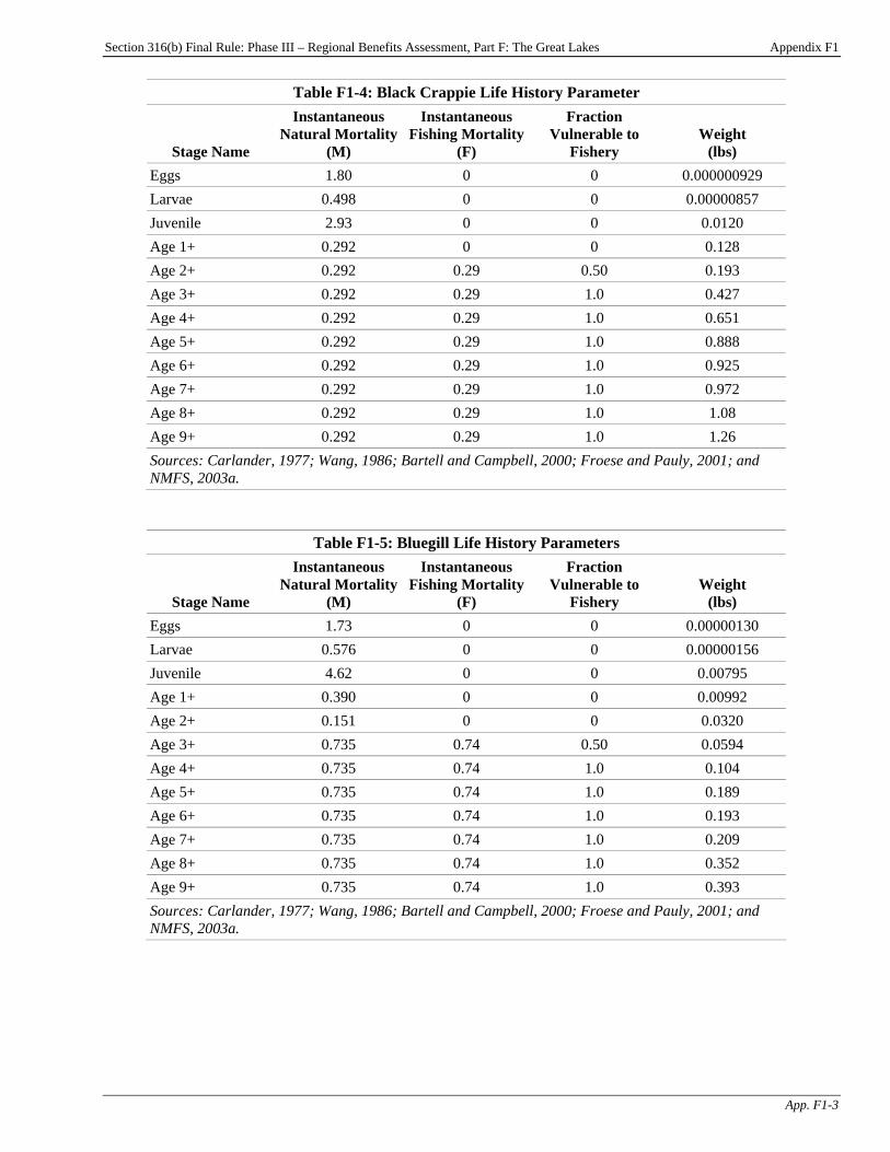
Section 316(b) Final Rule: Phase III – Regional Benefits Assessment, Part F: The Great Lakes Appendix F1
App. F1-3
Table F1-4: Black Crappie Life History Parameter
Stage Name
Instantaneous Natural Mortality
(M)
Instantaneous Fishing Mortality
(F)
Fraction Vulnerable to
Fishery Weight
(lbs) Eggs 1.80 0 0 0.000000929 Larvae 0.498 0 0 0.00000857 Juvenile 2.93 0 0 0.0120 Age 1+ 0.292 0 0 0.128 Age 2+ 0.292 0.29 0.50 0.193 Age 3+ 0.292 0.29 1.0 0.427 Age 4+ 0.292 0.29 1.0 0.651 Age 5+ 0.292 0.29 1.0 0.888 Age 6+ 0.292 0.29 1.0 0.925 Age 7+ 0.292 0.29 1.0 0.972 Age 8+ 0.292 0.29 1.0 1.08 Age 9+ 0.292 0.29 1.0 1.26 Sources: Carlander, 1977; Wang, 1986; Bartell and Campbell, 2000; Froese and Pauly, 2001; and NMFS, 2003a.
Table F1-5: Bluegill Life History Parameters
Stage Name
Instantaneous Natural Mortality
(M)
Instantaneous Fishing Mortality
(F)
Fraction Vulnerable to
Fishery Weight
(lbs) Eggs 1.73 0 0 0.00000130 Larvae 0.576 0 0 0.00000156 Juvenile 4.62 0 0 0.00795 Age 1+ 0.390 0 0 0.00992 Age 2+ 0.151 0 0 0.0320 Age 3+ 0.735 0.74 0.50 0.0594 Age 4+ 0.735 0.74 1.0 0.104 Age 5+ 0.735 0.74 1.0 0.189 Age 6+ 0.735 0.74 1.0 0.193 Age 7+ 0.735 0.74 1.0 0.209 Age 8+ 0.735 0.74 1.0 0.352 Age 9+ 0.735 0.74 1.0 0.393 Sources: Carlander, 1977; Wang, 1986; Bartell and Campbell, 2000; Froese and Pauly, 2001; and NMFS, 2003a.
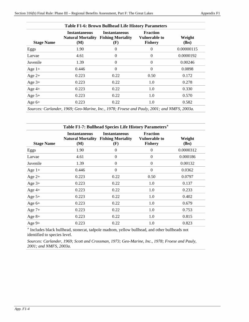
Section 316(b) Final Rule: Phase III – Regional Benefits Assessment, Part F: The Great Lakes Appendix F1
App. F1-4
Table F1-6: Brown Bullhead Life History Parameters
Stage Name
Instantaneous Natural Mortality
(M)
Instantaneous Fishing Mortality
(F)
Fraction Vulnerable to
Fishery Weight
(lbs) Eggs 1.90 0 0 0.00000115 Larvae 4.61 0 0 0.0000192 Juvenile 1.39 0 0 0.00246 Age 1+ 0.446 0 0 0.0898 Age 2+ 0.223 0.22 0.50 0.172 Age 3+ 0.223 0.22 1.0 0.278 Age 4+ 0.223 0.22 1.0 0.330 Age 5+ 0.223 0.22 1.0 0.570 Age 6+ 0.223 0.22 1.0 0.582 TSources: Carlander, 1969; Geo-Marine, Inc., 1978; Froese and Pauly, 2001; Tand NMFS, 2003a.
Table F1-7: Bullhead Species Life History ParametersP
aP
Stage Name
Instantaneous Natural Mortality
(M)
Instantaneous Fishing Mortality
(F)
Fraction Vulnerable to
Fishery Weight
(lbs) Eggs 1.90 0 0 0.0000312 Larvae 4.61 0 0 0.000186 Juvenile 1.39 0 0 0.00132 Age 1+ 0.446 0 0 0.0362 Age 2+ 0.223 0.22 0.50 0.0797 Age 3+ 0.223 0.22 1.0 0.137 Age 4+ 0.223 0.22 1.0 0.233 Age 5+ 0.223 0.22 1.0 0.402 Age 6+ 0.223 0.22 1.0 0.679 Age 7+ 0.223 0.22 1.0 0.753 Age 8+ 0.223 0.22 1.0 0.815 Age 9+ 0.223 0.22 1.0 0.823 P
aP Includes black bullhead, stonecat, tadpole madtom, yellow bullhead, and other bullheads not
identified to species level. Sources: Carlander, 1969; Scott and Crossman, 1973; Geo-Marine, Inc., 1978; Froese and Pauly, 2001; and NMFS, 2003a.
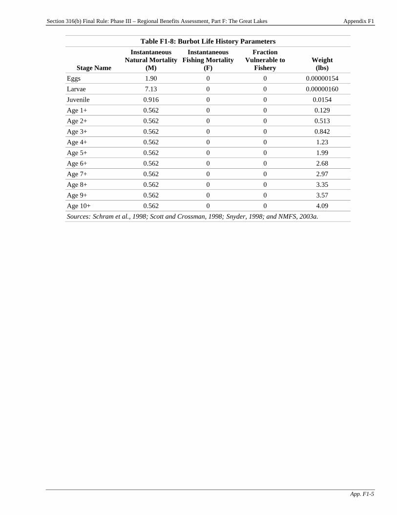
Section 316(b) Final Rule: Phase III – Regional Benefits Assessment, Part F: The Great Lakes Appendix F1
App. F1-5
Table F1-8: Burbot Life History Parameters
Stage Name
Instantaneous Natural Mortality
(M)
Instantaneous Fishing Mortality
(F)
Fraction Vulnerable to
Fishery Weight
(lbs) Eggs 1.90 0 0 0.00000154 Larvae 7.13 0 0 0.00000160 Juvenile 0.916 0 0 0.0154 Age 1+ 0.562 0 0 0.129 Age 2+ 0.562 0 0 0.513 Age 3+ 0.562 0 0 0.842 Age 4+ 0.562 0 0 1.23 Age 5+ 0.562 0 0 1.99 Age 6+ 0.562 0 0 2.68 Age 7+ 0.562 0 0 2.97 Age 8+ 0.562 0 0 3.35 Age 9+ 0.562 0 0 3.57 Age 10+ 0.562 0 0 4.09 Sources:T Schram et al., 1998; Scott and Crossman, 1998; TSnyder, 1998; and NMFS, 2003a.

Section 316(b) Final Rule: Phase III – Regional Benefits Assessment, Part F: The Great Lakes Appendix F1
App. F1-6
Table F1-9: Carp Life History ParametersP
aP
Stage Name
Instantaneous Natural Mortality
(M)
Instantaneous Fishing Mortality
(F)
Fraction Vulnerable to
Fishery Weight
(lbs) Eggs 1.90 0 0 0.00000673 Larvae 4.61 0 0 0.0000118 Juvenile 1.39 0 0 0.0225 Age 1+ 0.130 0 0 0.790 Age 2+ 0.130 0 0 1.21 Age 3+ 0.130 0 0 1.81 Age 4+ 0.130 0 0 5.13 Age 5+ 0.130 0 0 5.52 Age 6+ 0.130 0 0 5.82 Age 7+ 0.130 0 0 6.76 Age 8+ 0.130 0 0 8.17 Age 9+ 0.130 0 0 8.55 Age 10+ 0.130 0 0 8.94 Age 11+ 0.130 0 0 9.76 Age 12+ 0.130 0 0 10.2 Age 13+ 0.130 0 0 10.6 Age 14+ 0.130 0 0 11.1 Age 15+ 0.130 0 0 11.5 Age 16+ 0.130 0 0 12.0 Age 17+ 0.130 0 0 12.5 P
aP Includes bowfin, carp, goldfish, and other similar carps not identified to species level.
TSources: Carlander, 1969; Geo-Marine, Inc., 1978; Wang, 1986; Froese and Pauly, 2001; Tand NMFS, 2003a.
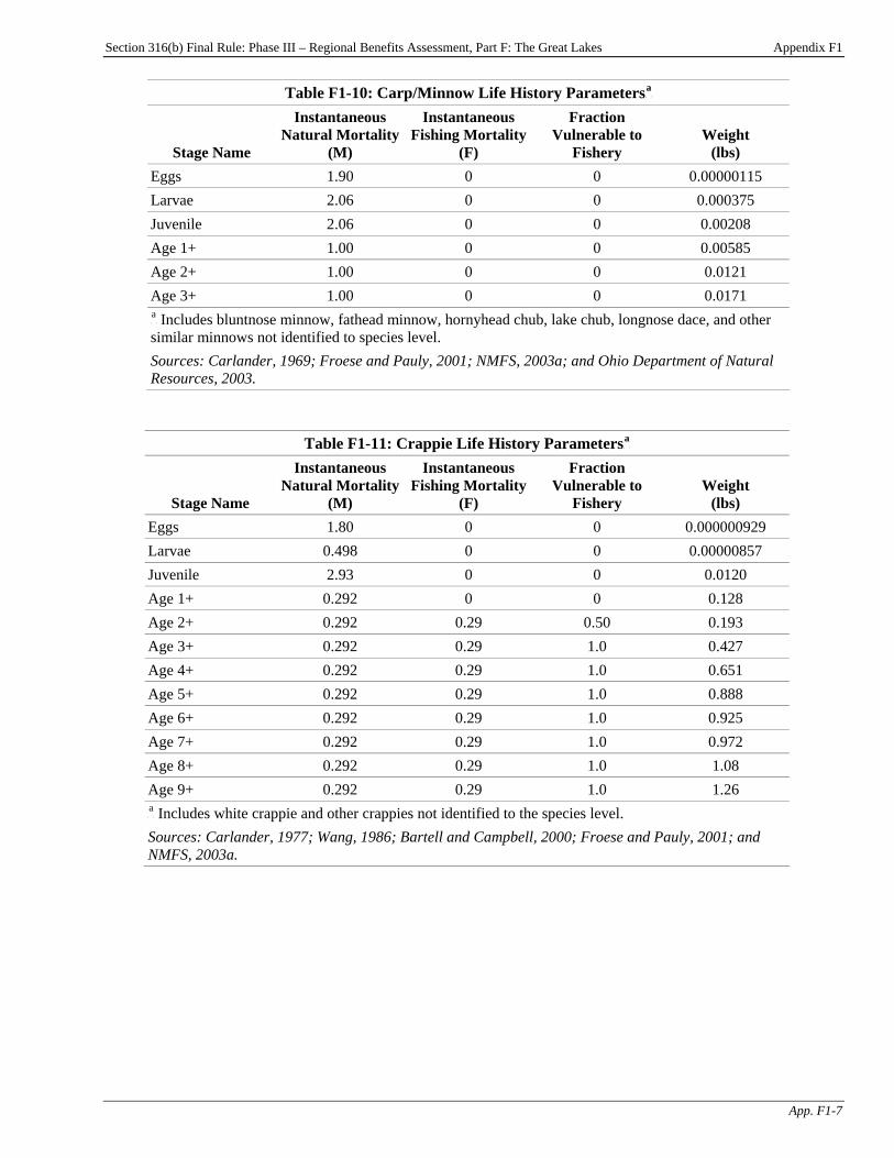
Section 316(b) Final Rule: Phase III – Regional Benefits Assessment, Part F: The Great Lakes Appendix F1
App. F1-7
Table F1-10: Carp/Minnow Life History ParametersP
aP
Stage Name
Instantaneous Natural Mortality
(M)
Instantaneous Fishing Mortality
(F)
Fraction Vulnerable to
Fishery Weight
(lbs) Eggs 1.90 0 0 0.00000115 Larvae 2.06 0 0 0.000375 Juvenile 2.06 0 0 0.00208 Age 1+ 1.00 0 0 0.00585 Age 2+ 1.00 0 0 0.0121 Age 3+ 1.00 0 0 0.0171 P
aP Includes bluntnose minnow, fathead minnow, hornyhead chub, lake chub, longnose dace, and other
similar minnows not identified to species level. Sources: Carlander, 1969; Froese and Pauly, 2001; NMFS, 2003a; and Ohio Department of Natural Resources, 2003.
Table F1-11: Crappie Life History ParametersP
aP
Stage Name
Instantaneous Natural Mortality
(M)
Instantaneous Fishing Mortality
(F)
Fraction Vulnerable to
Fishery Weight
(lbs) Eggs 1.80 0 0 0.000000929 Larvae 0.498 0 0 0.00000857 Juvenile 2.93 0 0 0.0120 Age 1+ 0.292 0 0 0.128 Age 2+ 0.292 0.29 0.50 0.193 Age 3+ 0.292 0.29 1.0 0.427 Age 4+ 0.292 0.29 1.0 0.651 Age 5+ 0.292 0.29 1.0 0.888 Age 6+ 0.292 0.29 1.0 0.925 Age 7+ 0.292 0.29 1.0 0.972 Age 8+ 0.292 0.29 1.0 1.08 Age 9+ 0.292 0.29 1.0 1.26 P
aP Includes white crappie and other crappies not identified to the species level.
Sources: Carlander, 1977; Wang, 1986; Bartell and Campbell, 2000; Froese and Pauly, 2001; and NMFS, 2003a.

Section 316(b) Final Rule: Phase III – Regional Benefits Assessment, Part F: The Great Lakes Appendix F1
App. F1-8
Table F1-12: Freshwater Catfish Life History ParametersP
aP
Stage Name
Instantaneous Natural Mortality
(M)
Instantaneous Fishing Mortality
(F)
Fraction Vulnerable to
Fishery Weight
(lbs) Eggs 1.90 0 0 0.0000539 Larvae 4.61 0 0 0.0000563 Juvenile 1.39 0 0 0.0204 Age 1+ 0.410 0.41 0.50 0.104 Age 2+ 0.410 0.41 1.0 0.330 Age 3+ 0.410 0.41 1.0 0.728 Age 4+ 0.410 0.41 1.0 1.15 Age 5+ 0.410 0.41 1.0 1.92 Age 6+ 0.410 0.41 1.0 2.41 Age 7+ 0.410 0.41 1.0 3.45 Age 8+ 0.410 0.41 1.0 4.01 Age 9+ 0.410 0.41 1.0 5.06 Age 10+ 0.410 0.41 1.0 8.08 Age 11+ 0.410 0.41 1.0 8.39 Age 12+ 0.410 0.41 1.0 8.53 P
aP Includes channel catfish and flathead catfish.
TSources: Miller, 1966; Carlander, 1969; Geo-Marine, Inc., 1978; Wang, 1986; Saila et al., 1997; Froese and Pauly, 2001; Tand NMFS, 2003a.
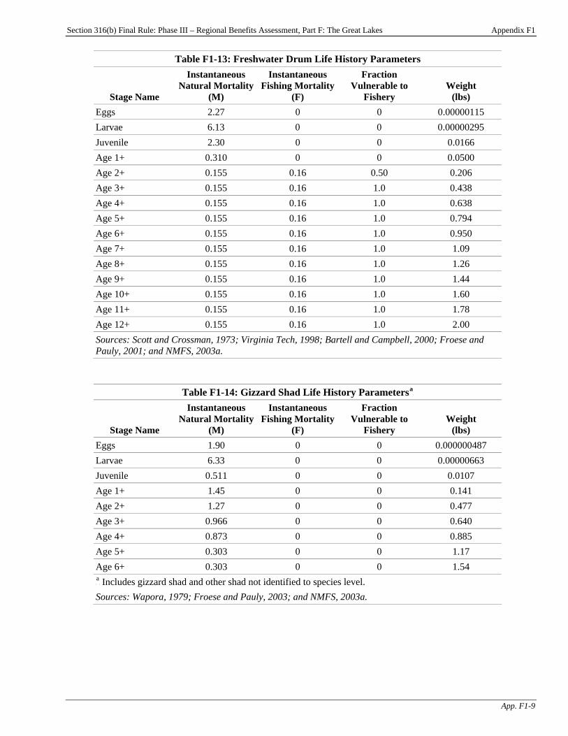
Section 316(b) Final Rule: Phase III – Regional Benefits Assessment, Part F: The Great Lakes Appendix F1
App. F1-9
Table F1-13: Freshwater Drum Life History Parameters
Stage Name
Instantaneous Natural Mortality
(M)
Instantaneous Fishing Mortality
(F)
Fraction Vulnerable to
Fishery Weight
(lbs) Eggs 2.27 0 0 0.00000115 Larvae 6.13 0 0 0.00000295 Juvenile 2.30 0 0 0.0166 Age 1+ 0.310 0 0 0.0500 Age 2+ 0.155 0.16 0.50 0.206 Age 3+ 0.155 0.16 1.0 0.438 Age 4+ 0.155 0.16 1.0 0.638 Age 5+ 0.155 0.16 1.0 0.794 Age 6+ 0.155 0.16 1.0 0.950 Age 7+ 0.155 0.16 1.0 1.09 Age 8+ 0.155 0.16 1.0 1.26 Age 9+ 0.155 0.16 1.0 1.44 Age 10+ 0.155 0.16 1.0 1.60 Age 11+ 0.155 0.16 1.0 1.78 Age 12+ 0.155 0.16 1.0 2.00 Sources: Scott and Crossman, 1973; Virginia Tech, 1998; Bartell and Campbell, 2000; Froese and Pauly, 2001; and NMFS, 2003a.
Table F1-14: Gizzard Shad Life History ParametersP
aP
Stage Name
Instantaneous Natural Mortality
(M)
Instantaneous Fishing Mortality
(F)
Fraction Vulnerable to
Fishery Weight
(lbs) Eggs 1.90 0 0 0.000000487 Larvae 6.33 0 0 0.00000663 Juvenile 0.511 0 0 0.0107 Age 1+ 1.45 0 0 0.141 Age 2+ 1.27 0 0 0.477 Age 3+ 0.966 0 0 0.640 Age 4+ 0.873 0 0 0.885 Age 5+ 0.303 0 0 1.17 Age 6+ 0.303 0 0 1.54 P
aP Includes gizzard shad and other shad not identified to species level.
Sources: Wapora, 1979; Froese and Pauly, 2003; and NMFS, 2003a.
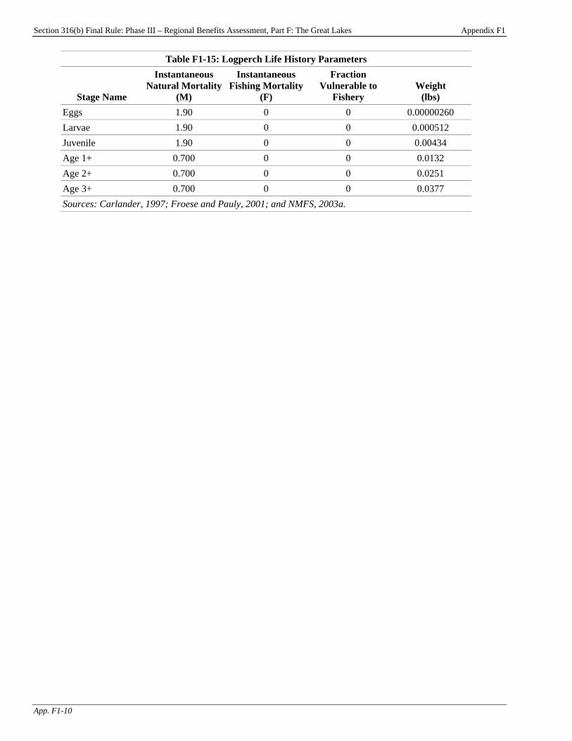
Section 316(b) Final Rule: Phase III – Regional Benefits Assessment, Part F: The Great Lakes Appendix F1
App. F1-10
Table F1-15: Logperch Life History Parameters
Stage Name
Instantaneous Natural Mortality
(M)
Instantaneous Fishing Mortality
(F)
Fraction Vulnerable to
Fishery Weight
(lbs) Eggs 1.90 0 0 0.00000260 Larvae 1.90 0 0 0.000512 Juvenile 1.90 0 0 0.00434 Age 1+ 0.700 0 0 0.0132 Age 2+ 0.700 0 0 0.0251 Age 3+ 0.700 0 0 0.0377 Sources: Carlander, 1997; Froese and Pauly, 2001; and NMFS, 2003a.
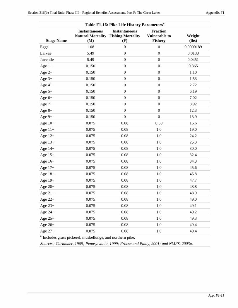
Section 316(b) Final Rule: Phase III – Regional Benefits Assessment, Part F: The Great Lakes Appendix F1
App. F1-11
Table F1-16: Pike Life History ParametersP
aP
Stage Name
Instantaneous Natural Mortality
(M)
Instantaneous Fishing Mortality
(F)
Fraction Vulnerable to
Fishery Weight
(lbs) Eggs 1.08 0 0 0.0000189 Larvae 5.49 0 0 0.0133 Juvenile 5.49 0 0 0.0451 Age 1+ 0.150 0 0 0.365 Age 2+ 0.150 0 0 1.10 Age 3+ 0.150 0 0 1.53 Age 4+ 0.150 0 0 2.72 Age 5+ 0.150 0 0 6.19 Age 6+ 0.150 0 0 7.02 Age 7+ 0.150 0 0 8.92 Age 8+ 0.150 0 0 12.3 Age 9+ 0.150 0 0 13.9 Age 10+ 0.075 0.08 0.50 16.6 Age 11+ 0.075 0.08 1.0 19.0 Age 12+ 0.075 0.08 1.0 24.2 Age 13+ 0.075 0.08 1.0 25.3 Age 14+ 0.075 0.08 1.0 30.0 Age 15+ 0.075 0.08 1.0 32.4 Age 16+ 0.075 0.08 1.0 34.3 Age 17+ 0.075 0.08 1.0 45.6 Age 18+ 0.075 0.08 1.0 45.8 Age 19+ 0.075 0.08 1.0 47.7 Age 20+ 0.075 0.08 1.0 48.8 Age 21+ 0.075 0.08 1.0 48.9 Age 22+ 0.075 0.08 1.0 49.0 Age 23+ 0.075 0.08 1.0 49.1 Age 24+ 0.075 0.08 1.0 49.2 Age 25+ 0.075 0.08 1.0 49.3 Age 26+ 0.075 0.08 1.0 49.4 Age 27+ 0.075 0.08 1.0 49.4 P
aP Includes grass pickerel, muskellunge, and northern pike.
TSources: Carlander, 1969T; Pennsylvania, 1999; Froese and Pauly, 2001; and NMFS, 2003a.

Section 316(b) Final Rule: Phase III – Regional Benefits Assessment, Part F: The Great Lakes Appendix F1
App. F1-12
Table F1-17: Rainbow Smelt Life History Parameters
Stage Name
Instantaneous Natural Mortality
(M)
Instantaneous Fishing Mortality
(F)
Fraction Vulnerable to
Fishery Weight
(lbs) Eggs 11.5 0 0 0.000000990 Larvae 5.50 0 0 0.00110 Juvenile 0.916 0 0 0.00395 Age 1+ 0.400 0 0 0.0182 Age 2+ 0.400 0.03 0.50 0.0460 Age 3+ 0.400 0.03 1.0 0.0850 Age 4+ 0.400 0.03 1.0 0.131 Age 5+ 0.400 0.03 1.0 0.180 Age 6+ 0.400 0.03 1.0 0.228 Sources: Spigarelli et al., 1981; PG&E National Energy Group, 2001; Froese and Pauly, 2003; and NMFS, 2003a.
Table F1-18: Redhorse Species Life History ParametersP
aP
Stage Name
Instantaneous Natural Mortality
(M)
Instantaneous Fishing Mortality
(F)
Fraction Vulnerable to
Fishery Weight
(lbs) Eggs 2.30 0 0 0.00000115 Larvae 2.30 0 0 0.00000370 Juvenile 2.99 0 0 0.0267 Age 1+ 0.548 0 0 0.0521 Age 2+ 0.548 0 0 0.180 Age 3+ 0.548 0 0 0.493 Age 4+ 0.548 0 0 0.653 Age 5+ 0.548 0 0 0.916 Age 6+ 0.548 0 0 2.78 Age 7+ 0.548 0 0 3.07 P
aP Includes golden redhorse, shorthead redhorse, and silver redhorse.
Sources: Carlander, 1969; Bartell and Campbell, 2000; Froese and Pauly, 2001, 2003; and NMFS, 2003a.

Section 316(b) Final Rule: Phase III – Regional Benefits Assessment, Part F: The Great Lakes Appendix F1
App. F1-13
Table F1-19: Salmonids Life History ParametersP
aP
Stage Name
Instantaneous Natural Mortality
(M)
Instantaneous Fishing Mortality
(F)
Fraction Vulnerable to Fishery
Weight (lbs)
Eggs 1.90 0 0 0.0000240 Larvae 8.20 0 0 0.000171 Juvenile 0.250 0 0 0.0117 Age 1+ 0.250 1.0 0.50 0.705 Age 2+ 0.250 1.0 1.0 1.27 Age 3+ 0.250 1.0 1.0 2.32 Age 4+ 0.250 1.0 1.0 2.85 Age 5+ 0.250 1.0 1.0 3.52 Age 6+ 0.250 1.0 1.0 4.09 Age 7+ 0.250 1.0 1.0 4.76 Age 8+ 0.250 1.0 1.0 5.70 Age 9+ 0.250 1.0 1.0 5.73 Age 10+ 0.250 1.0 1.0 5.85 Age 11+ 0.250 1.0 1.0 6.10 Age 12+ 0.250 1.0 1.0 6.83 Age 13+ 0.250 1.0 1.0 7.11 Age 14+ 0.250 1.0 1.0 7.29 Age 15+ 0.250 1.0 1.0 7.32 Age 16+ 0.250 1.0 1.0 8.66 P
aP IncludesP
Pbloater, brown trout, chinook salmon, coho salmon, lake herring, lake trout, lake whitefish,
rainbow trout, round whitefish, and other salmonids not identified to species level.
Sources: Fish, 1932; Schorfhaar and Schneeberger, 1997; Scott and Crossman, 1998; Froese and Pauly, 2001; and NMFS, 2003a.
Table F1-20: Shiner Species Life History ParametersP
aP
Stage Name
Instantaneous Natural Mortality
(M)
Instantaneous Fishing Mortality
(F)
Fraction Vulnerable to
Fishery Weight
(lbs) Eggs 1.90 0 0 0.00000473 Larvae 4.61 0 0 0.000285 Juvenile 0.777 0 0 0.00209 Age 1+ 0.371 0 0 0.00387 Age 2+ 4.61 0 0 0.00683 Age 3+ 4.61 0 0 0.0143 P
aP Includes common shiner, emerald shiner, golden shiner, spotfin shiner, spottail shiner, and other
shiners not identified to species level. TSources: Fuchs, 1967; Wapora, 1979; Trautman, 1981; Froese and Pauly, 2003; and NMFS, 2003a.T
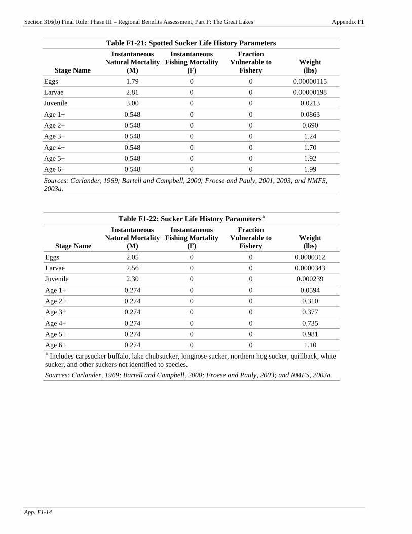
Section 316(b) Final Rule: Phase III – Regional Benefits Assessment, Part F: The Great Lakes Appendix F1
App. F1-14
Table F1-21: Spotted Sucker Life History Parameters
Stage Name
Instantaneous Natural Mortality
(M)
Instantaneous Fishing Mortality
(F)
Fraction Vulnerable to
Fishery Weight
(lbs) Eggs 1.79 0 0 0.00000115 Larvae 2.81 0 0 0.00000198 Juvenile 3.00 0 0 0.0213 Age 1+ 0.548 0 0 0.0863 Age 2+ 0.548 0 0 0.690 Age 3+ 0.548 0 0 1.24 Age 4+ 0.548 0 0 1.70 Age 5+ 0.548 0 0 1.92 Age 6+ 0.548 0 0 1.99 Sources: Carlander, 1969; Bartell and Campbell, 2000; Froese and Pauly, 2001, 2003; and NMFS, 2003a.
Table F1-22: Sucker Life History ParametersP
aP
Stage Name
Instantaneous Natural Mortality
(M)
Instantaneous Fishing Mortality
(F)
Fraction Vulnerable to
Fishery Weight
(lbs) Eggs 2.05 0 0 0.0000312 Larvae 2.56 0 0 0.0000343 Juvenile 2.30 0 0 0.000239 Age 1+ 0.274 0 0 0.0594 Age 2+ 0.274 0 0 0.310 Age 3+ 0.274 0 0 0.377 Age 4+ 0.274 0 0 0.735 Age 5+ 0.274 0 0 0.981 Age 6+ 0.274 0 0 1.10 P
aP Includes carpsucker buffalo, lake chubsucker, longnose sucker, northern hog sucker, quillback, white
sucker, and other suckers not identified to species. Sources: Carlander, 1969; Bartell and Campbell, 2000; Froese and Pauly, 2003; and NMFS, 2003a.
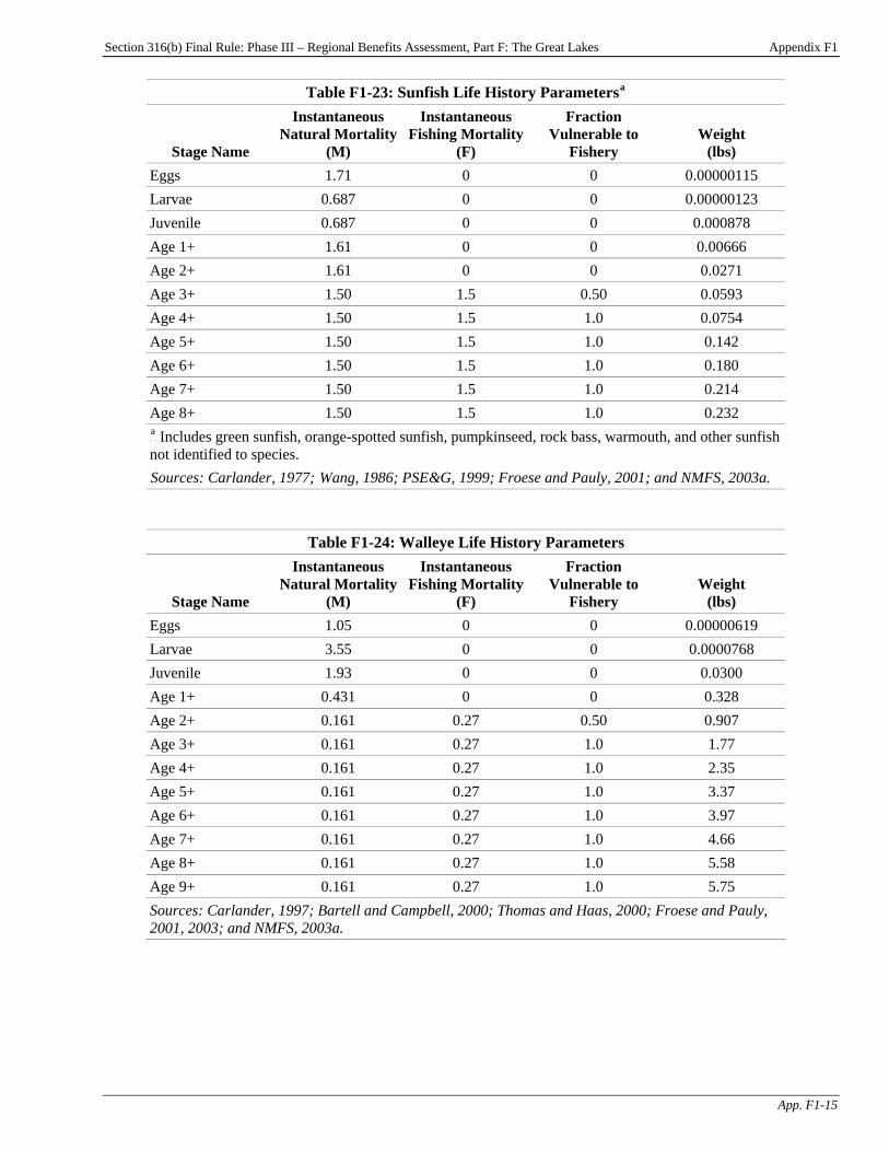
Section 316(b) Final Rule: Phase III – Regional Benefits Assessment, Part F: The Great Lakes Appendix F1
App. F1-15
Table F1-23: Sunfish Life History ParametersP
aP
Stage Name
Instantaneous Natural Mortality
(M)
Instantaneous Fishing Mortality
(F)
Fraction Vulnerable to
Fishery Weight
(lbs) Eggs 1.71 0 0 0.00000115 Larvae 0.687 0 0 0.00000123 Juvenile 0.687 0 0 0.000878 Age 1+ 1.61 0 0 0.00666 Age 2+ 1.61 0 0 0.0271 Age 3+ 1.50 1.5 0.50 0.0593 Age 4+ 1.50 1.5 1.0 0.0754 Age 5+ 1.50 1.5 1.0 0.142 Age 6+ 1.50 1.5 1.0 0.180 Age 7+ 1.50 1.5 1.0 0.214 Age 8+ 1.50 1.5 1.0 0.232 P
aP Includes green sunfish, orange-spotted sunfish, pumpkinseed, rock bass, warmouth, and other sunfish
not identified to species. TSources: Carlander, 1977; TWang, 1986; PSE&G, 1999; Froese and Pauly, 2001; and NMFS, 2003a.
Table F1-24: Walleye Life History Parameters
Stage Name
Instantaneous Natural Mortality
(M)
Instantaneous Fishing Mortality
(F)
Fraction Vulnerable to
Fishery Weight
(lbs) Eggs 1.05 0 0 0.00000619 Larvae 3.55 0 0 0.0000768 Juvenile 1.93 0 0 0.0300 Age 1+ 0.431 0 0 0.328 Age 2+ 0.161 0.27 0.50 0.907 Age 3+ 0.161 0.27 1.0 1.77 Age 4+ 0.161 0.27 1.0 2.35 Age 5+ 0.161 0.27 1.0 3.37 Age 6+ 0.161 0.27 1.0 3.97 Age 7+ 0.161 0.27 1.0 4.66 Age 8+ 0.161 0.27 1.0 5.58 Age 9+ 0.161 0.27 1.0 5.75 Sources: Carlander, 1997; Bartell and Campbell, 2000; Thomas and Haas, 2000; Froese and Pauly, 2001, 2003; and NMFS, 2003a.

Section 316(b) Final Rule: Phase III – Regional Benefits Assessment, Part F: The Great Lakes Appendix F1
App. F1-16
Table F1-25: White Bass Life History Parameters
Stage Name
Instantaneous Natural Mortality
(M)
Instantaneous Fishing Mortality
(F)
Fraction Vulnerable to
Fishery Weight
(lbs) Eggs 1.90 0 0 0.000000396 Larvae 4.61 0 0 0.00000174 Juvenile 1.39 0 0 0.174 Age 1+ 0.420 0 0 0.467 Age 2+ 0.420 0.70 0.50 0.644 Age 3+ 0.420 0.70 1.0 1.02 Age 4+ 0.420 0.70 1.0 1.16 Age 5+ 0.420 0.70 1.0 1.26 Age 6+ 0.420 0.70 1.0 1.66 Age 7+ 0.420 0.70 1.0 1.68 TSources: Van Oosten, 1942; Geo-Marine, Inc., 1978; Carlander, 1997; Virginia Tech, 1998; McDermot and Rose, 2000; Froese and Pauly, 2001; Tand NMFS, 2003a.
Table F1-26: White Perch Life History Parameters
Stage Name
Instantaneous Natural Mortality
(M)
Instantaneous Fishing Mortality
(F)
Fraction Vulnerable to
Fishery Weight
(lbs) Eggs 2.75 0 0 0.000000330 Larvae 5.37 0 0 0.00000271 Juvenile 1.71 0 0 0.00259 Age 1+ 0.693 0 0 0.0198 Age 2+ 0.693 0 0 0.0567 Age 3+ 0.693 0 0 0.103 Age 4+ 0.689 0 0 0.150 Age 5+ 1.58 0 0 0.214 Age 6+ 1.54 0 0 0.265 Age 7+ 1.48 0 0 0.356 Age 8+ 1.46 0 0 0.387 Age 9+ 1.46 0 0 0.516 Age 10+ 1.46 0 0 0.619 TSources: Horseman and Shirey, 1974; PSE&G, 1999; and NMFS, 2003a.T
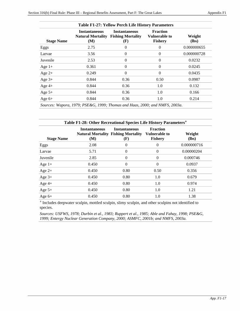
Section 316(b) Final Rule: Phase III – Regional Benefits Assessment, Part F: The Great Lakes Appendix F1
App. F1-17
Table F1-27: Yellow Perch Life History Parameters
Stage Name
Instantaneous Natural Mortality
(M)
Instantaneous Fishing Mortality
(F)
Fraction Vulnerable to
Fishery Weight
(lbs) Eggs 2.75 0 0 0.000000655 Larvae 3.56 0 0 0.000000728 Juvenile 2.53 0 0 0.0232 Age 1+ 0.361 0 0 0.0245 Age 2+ 0.249 0 0 0.0435 Age 3+ 0.844 0.36 0.50 0.0987 Age 4+ 0.844 0.36 1.0 0.132 Age 5+ 0.844 0.36 1.0 0.166 Age 6+ 0.844 0.36 1.0 0.214 Sources:T Wapora, 1979; PSE&G, 1999T; Thomas and Haas, 2000; and NMFS, 2003a.
Table F1-28: Other Recreational Species Life History ParametersP
aP
Stage Name
Instantaneous Natural Mortality
(M)
Instantaneous Fishing Mortality
(F)
Fraction Vulnerable to
Fishery Weight
(lbs) Eggs 2.08 0 0 0.000000716 Larvae 5.71 0 0 0.00000204 Juvenile 2.85 0 0 0.000746 Age 1+ 0.450 0 0 0.0937 Age 2+ 0.450 0.80 0.50 0.356 Age 3+ 0.450 0.80 1.0 0.679 Age 4+ 0.450 0.80 1.0 0.974 Age 5+ 0.450 0.80 1.0 1.21 Age 6+ 0.450 0.80 1.0 1.38 P
aP Includes deepwater sculpin, mottled sculpin, slimy sculpin, and other sculpins not identified to
species. Sources: USFWS, 1978; Durbin et al., 1983; Ruppert et al., 1985; Able and Fahay, 1998; PSE&G, 1999; Entergy Nuclear Generation Company, 2000; ASMFC, 2001b; and NMFS, 2003a.

Section 316(b) Final Rule: Phase III – Regional Benefits Assessment, Part F: The Great Lakes Appendix F1
App. F1-18
Table F1-29: Other Forage Species Life History ParametersP
aP
Stage Name
Instantaneous Natural Mortality
(M)
Instantaneous Fishing Mortality
(F)
Fraction Vulnerable to
Fishery Weight
(lbs) Eggs 1.04 0 0 0.0000000186 Larvae 7.70 0 0 0.00000158 Juvenile 1.29 0 0 0.000481 Age 1+ 1.62 0 0 0.00381 Age 2+ 1.62 0 0 0.00496 Age 3+ 1.62 0 0 0.00505 P
aP Includes central mudminnow, chestnut lamprey, johnny darter, lake sturgeon, longnose gar,
ninespine stickleback, pirate perch, sea lamprey, silver lamprey, and other forage fish not identified to species. Sources: Derickson and Price, 1973; and PSE&G, 1999.

Section 316(b) Final Rule: Phase III – Regional Benefits Assessment, Part F: The Great Lakes Chapter F2
F2-1
Chapter F2: Evaluation of Impingement and Entrainment in the Great Lakes Region
Background: The Great Lakes Fisheries Great Lakes fisheries are among the most important in the world, providing $4 billion in landings and recreation for some 5 million recreational anglers (Great Lakes Fishery Commission, 2003). Historically, the top predators in the Great Lakes included lake trout (Salvelinus namaycush), sturgeon (Acipenser fulvescens), lake whitefish (Coregonus clupeaformis), northern pike (Esox lucius), walleye (Sander vitreus), and muskellunge (Esox masquinongy). Today, as a result of numerous stressors such as habitat destruction, damming, and the introduction of sea lamprey and other exotic species, dominant species are primarily non-native salmon sustained by hatcheries. Not all introductions have been harmful, however. For example, alewife (Alosa pseudoharengus) was introduced to provide forage for sport fish (Jude et al., 1987). Losses of alewife, emerald shiner (Notropis atherinoides), and other forage species to impingement and entrainment (I&E) at Great Lakes facilities are sometimes substantial. Impinged and entrained species of commercial and/or recreational importance include yellow perch (Perca flavescens), white bass (Morone chrysops), gizzard shad (Dorosoma cepedianum), and walleye (Sander vitreus). F2-1 I&E Species/Species Groups Evaluated Table F2-1 provides a list of species/species groups that were evaluated in EPA’s analysis of I&E in the Great Lakes.
Table F2-1: Species/Species Group Evaluated by EPA that are Subject to I&E in the Great Lakes Region
Species/Species Group Recreational Commercial Forage Alewife X Black bullhead X Black crappie X Bluegill X Bluntnose minnow X Brown bullhead X Bullhead species X Burbot X Carp X Channel catfish X X
Chapter Contents F2-1 I&E Species/Species Groups Evaluated ....... F2-1 F2-2 I&E Data Evaluated ...................................... F2-3 F2-3 EPA’s Estimate of Current I&E at Phase III Facilities in the Great Lakes Region Expressed as Age-1 Equivalents and Foregone Yield ............................................. F2-3 F2-4 Reductions in I&E at Phase III Facilities in the Great Lakes Region Under Alternative Options....................................... F2-6 F2-5 Assumptions Used in Calculating Recreational and Commercial Losses ........... F2-6
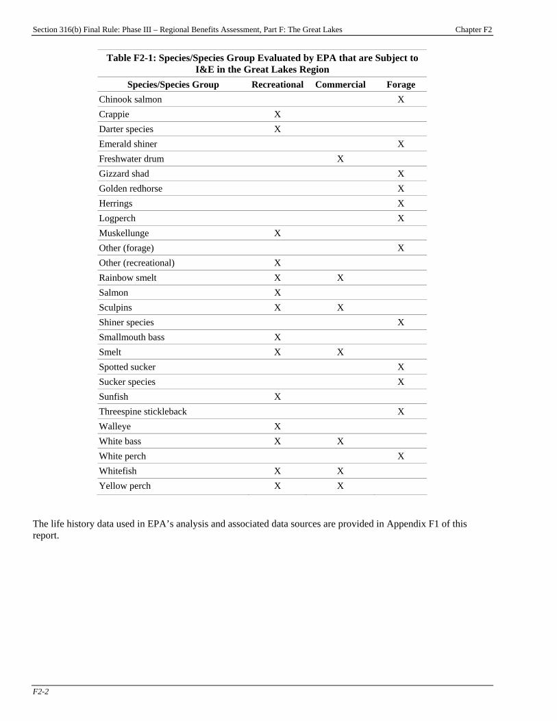
Section 316(b) Final Rule: Phase III – Regional Benefits Assessment, Part F: The Great Lakes Chapter F2
F2-2
Table F2-1: Species/Species Group Evaluated by EPA that are Subject to I&E in the Great Lakes Region
Species/Species Group Recreational Commercial Forage Chinook salmon X Crappie X Darter species X Emerald shiner X Freshwater drum X Gizzard shad X Golden redhorse X Herrings X Logperch X Muskellunge X Other (forage) X Other (recreational) X Rainbow smelt X X Salmon X Sculpins X X Shiner species X Smallmouth bass X Smelt X X Spotted sucker X Sucker species X Sunfish X Threespine stickleback X Walleye X White bass X X White perch X Whitefish X X Yellow perch X X
The life history data used in EPA’s analysis and associated data sources are provided in Appendix F1 of this report.

Section 316(b) Final Rule: Phase III – Regional Benefits Assessment, Part F: The Great Lakes Chapter F2
F2-3
F2-2 I&E Data Evaluated Table F2-2 lists the facility I&E data evaluated by EPA to estimate current I&E rates for the region. See Chapter A1 of Part A for a discussion of the methods used to evaluate the I&E data. The facility studies used in EPA’s analysis are provided in the 316(b) docket.
Table F2-2: Facility I&E Data Evaluated for the Great Lakes Region Facilities Phase Years of Data
Bailly Generating Station II 1975 D.H. Mitchell Station II 1975 DC Cook Nuclear Power Plant II 1975-1982 J.P. Pulliam Power Plant II 1975 J.R. Whiting Power Plant II 1978-1991 Monroe Power Plant II 1974-1985 Pleasant Prairie Power Plant III 1980 Port Washington Power Plant II 1975-1980 Silver Bay Power Plant III 1981 South Oak Creek II 1975 U.S. Steel Corporation Gary Works III 1977
F2-3 EPA’s Estimate of Current I&E at Phase III Facilities in the Great Lakes Region
Expressed as Age-1 Equivalents and Foregone Yield Table F2-3 provides EPA’s estimate of the annual age-1 equivalents and foregone fishery yield resulting from the impingement of aquatic species at facilities located in the Great Lakes region. Table F2-4 displays this information for entrainment. Note that in these tables, “total yield” includes direct losses of harvested species and the yield of harvested species that is lost due to losses of forage species (trophic transfer).
Table F2-3: Estimated Current Annual Impingement at Phase III Facilities in the Great Lakes Region Expressed as Age-1 Equivalents and
Foregone Fishery Yield
Species/Species Group Age-1 Equivalents
(#s) Total Yield
(lbs) Alewife 31,600 <1 Black bullhead 14,300 1,130 Black crappie 74 12 Bluegill 33 1 Bluntnose minnow 533 <1 Brown bullhead 344 28 Bullhead species 676 55 Burbot 612 <1 Carp 5,720 <1

Section 316(b) Final Rule: Phase III – Regional Benefits Assessment, Part F: The Great Lakes Chapter F2
F2-4
Table F2-3: Estimated Current Annual Impingement at Phase III Facilities in the Great Lakes Region Expressed as Age-1 Equivalents and
Foregone Fishery Yield
Species/Species Group Age-1 Equivalents
(#s) Total Yield
(lbs) Channel catfish 2,070 429 Chinook salmon 364 <1 Crappie 165 28 Darter species 463 <1 Emerald shiner 3,030,000 <1 Freshwater drum 43,500 10,500 Gizzard shad 16,300,000 <1 Golden redhorse 19 <1 Herrings <1 <1 Logperch 31,700 <1 Muskellunge 6 23 Other (forage) 10,400 <1 Other (recreational) 7,610 1,500 Rainbow smelt 59,400 221 Salmon 668 2,820 Sculpins 252 17 Shiner species 7,310,000 <1 Smallmouth bass 434 18 Smelts 577,000 14,300 Spotted sucker <1 <1 Sucker species 948 <1 Sunfish 14,700 11 Threespine stickleback 4,470 <1 Trophic transferP
aP <1 145,000
Walleye 4,550 4,060 White bass 167,000 51,200 White perch 156,000 <1 Whitefish 30,200 27,100 Yellow perch 182,000 2,530 P
aP Contribution of forage fish to yield based on trophic transfer (see Chapter A1).
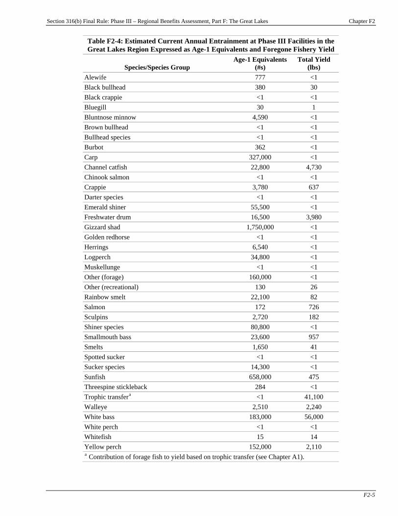
Section 316(b) Final Rule: Phase III – Regional Benefits Assessment, Part F: The Great Lakes Chapter F2
F2-5
Table F2-4: Estimated Current Annual Entrainment at Phase III Facilities in the Great Lakes Region Expressed as Age-1 Equivalents and Foregone Fishery Yield
Species/Species Group Age-1 Equivalents
(#s) Total Yield
(lbs) Alewife 777 <1 Black bullhead 380 30 Black crappie <1 <1 Bluegill 30 1 Bluntnose minnow 4,590 <1 Brown bullhead <1 <1 Bullhead species <1 <1 Burbot 362 <1 Carp 327,000 <1 Channel catfish 22,800 4,730 Chinook salmon <1 <1 Crappie 3,780 637 Darter species <1 <1 Emerald shiner 55,500 <1 Freshwater drum 16,500 3,980 Gizzard shad 1,750,000 <1 Golden redhorse <1 <1 Herrings 6,540 <1 Logperch 34,800 <1 Muskellunge <1 <1 Other (forage) 160,000 <1 Other (recreational) 130 26 Rainbow smelt 22,100 82 Salmon 172 726 Sculpins 2,720 182 Shiner species 80,800 <1 Smallmouth bass 23,600 957 Smelts 1,650 41 Spotted sucker <1 <1 Sucker species 14,300 <1 Sunfish 658,000 475 Threespine stickleback 284 <1 Trophic transferP
aP <1 41,100
Walleye 2,510 2,240 White bass 183,000 56,000 White perch <1 <1 Whitefish 15 14 Yellow perch 152,000 2,110 P
aP Contribution of forage fish to yield based on trophic transfer (see Chapter A1).
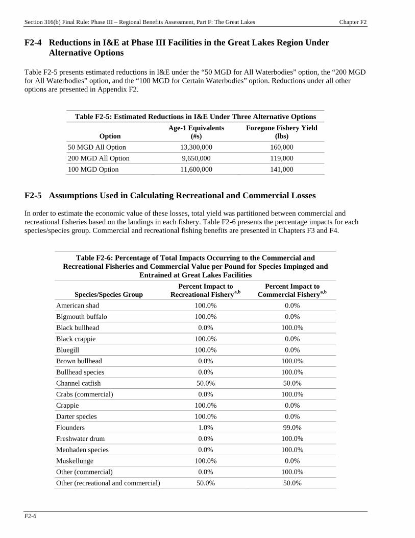
Section 316(b) Final Rule: Phase III – Regional Benefits Assessment, Part F: The Great Lakes Chapter F2
F2-6
F2-4 Reductions in I&E at Phase III Facilities in the Great Lakes Region Under Alternative Options
Table F2-5 presents estimated reductions in I&E under the “50 MGD for All Waterbodies” option, the “200 MGD for All Waterbodies” option, and the “100 MGD for Certain Waterbodies” option. Reductions under all other options are presented in Appendix F2.
Table F2-5: Estimated Reductions in I&E Under Three Alternative Options
Option Age-1 Equivalents
(#s) Foregone Fishery Yield
(lbs) 50 MGD All Option 13,300,000 160,000 200 MGD All Option 9,650,000 119,000 100 MGD Option 11,600,000 141,000
F2-5 Assumptions Used in Calculating Recreational and Commercial Losses In order to estimate the economic value of these losses, total yield was partitioned between commercial and recreational fisheries based on the landings in each fishery. Table F2-6 presents the percentage impacts for each species/species group. Commercial and recreational fishing benefits are presented in Chapters F3 and F4.
Table F2-6: Percentage of Total Impacts Occurring to the Commercial and Recreational Fisheries and Commercial Value per Pound for Species Impinged and
Entrained at Great Lakes Facilities
Species/Species Group Percent Impact to
Recreational FisheryP
a,bP
Percent Impact to Commercial FisheryP
a,bP
American shad 100.0% 0.0% Bigmouth buffalo 100.0% 0.0% Black bullhead 0.0% 100.0% Black crappie 100.0% 0.0% Bluegill 100.0% 0.0% Brown bullhead 0.0% 100.0% Bullhead species 0.0% 100.0% Channel catfish 50.0% 50.0% Crabs (commercial) 0.0% 100.0% Crappie 100.0% 0.0% Darter species 100.0% 0.0% Flounders 1.0% 99.0% Freshwater drum 0.0% 100.0% Menhaden species 0.0% 100.0% Muskellunge 100.0% 0.0% Other (commercial) 0.0% 100.0% Other (recreational and commercial) 50.0% 50.0%
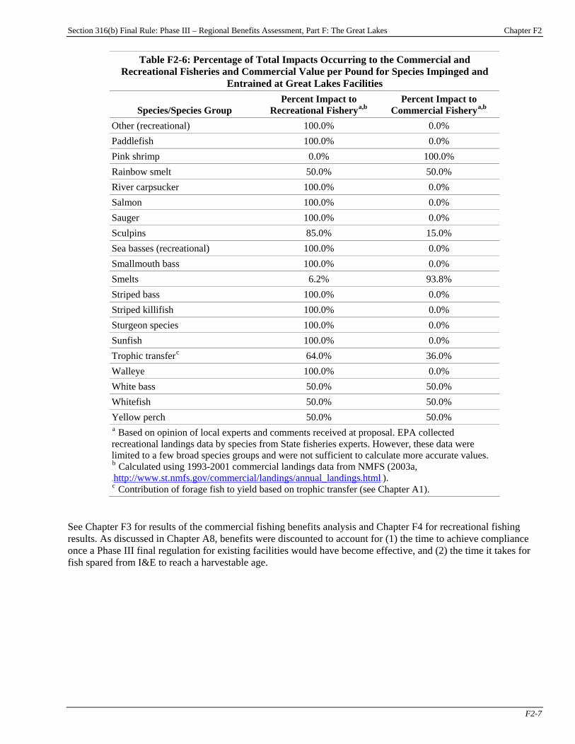
Section 316(b) Final Rule: Phase III – Regional Benefits Assessment, Part F: The Great Lakes Chapter F2
F2-7
Table F2-6: Percentage of Total Impacts Occurring to the Commercial and Recreational Fisheries and Commercial Value per Pound for Species Impinged and
Entrained at Great Lakes Facilities
Species/Species Group Percent Impact to
Recreational FisheryP
a,bP
Percent Impact to Commercial FisheryP
a,bP
Other (recreational) 100.0% 0.0% Paddlefish 100.0% 0.0% Pink shrimp 0.0% 100.0% Rainbow smelt 50.0% 50.0% River carpsucker 100.0% 0.0% Salmon 100.0% 0.0% Sauger 100.0% 0.0% Sculpins 85.0% 15.0% Sea basses (recreational) 100.0% 0.0% Smallmouth bass 100.0% 0.0% Smelts 6.2% 93.8% Striped bass 100.0% 0.0% Striped killifish 100.0% 0.0% Sturgeon species 100.0% 0.0% Sunfish 100.0% 0.0% Trophic transferP
cP 64.0% 36.0%
Walleye 100.0% 0.0% White bass 50.0% 50.0% Whitefish 50.0% 50.0% Yellow perch 50.0% 50.0% P
aP Based on opinion of local experts and comments received at proposal. EPA collected
recreational landings data by species from State fisheries experts. However, these data were limited to a few broad species groups and were not sufficient to calculate more accurate values. P
bP Calculated using 1993-2001 commercial landings data from NMFS (2003a,
HTUhttp://www.st.nmfs.gov/commercial/landings/annual_landings.htmlUTH). P
cP Contribution of forage fish to yield based on trophic transfer (see Chapter A1).
See Chapter F3 for results of the commercial fishing benefits analysis and Chapter F4 for recreational fishing results. As discussed in Chapter A8, benefits were discounted to account for (1) the time to achieve compliance once a Phase III final regulation for existing facilities would have become effective, and (2) the time it takes for fish spared from I&E to reach a harvestable age.

Section 316(b) Final Rule: Phase III – Regional Benefits Assessment, Part F: The Great Lakes Appendix F2
App. F2-1
Appendix F2: Reductions in I&E Under Supplemental Policy Options
Table F2-1: Estimated Reductions in I&E in the Great Lakes Region Under Eight Supplemental Options
Option Age-1 Equivalents
(#s) Foregone Fishery Yield
(lbs) Electric Generators 2-50 MGD
I-only Everywhere 303,000 2,820 I&E like Phase II 327,000 3,610 I&E Everywhere 331,000 3,740
Manufacturers 2-50 MGD I-only Everywhere 698,000 6,510 I&E like Phase II 732,000 7,580 I&E Everywhere 764,000 8,620
Manufacturers 50+ MGD I-only Everywhere 11,700,000 109,000 I&E Everywhere 13,400,000 161,000
Section 316(b) Final Rule: Phase III – Regional Benefits Assessment, Part F: The Great Lakes Chapter F3
F3-1
Chapter F3: Commercial Fishing Benefits Introduction
Chapter Contents F3-1 Baseline Commercial Losses.........................F3-1 F3-2 Expected Benefits Under Regulatory Analysis Options ...........................................F3-3
F3-2.1 Commercial Fishing Benefits of the “50 MGD for All Waterbodies” Option ..............................................F3-3 F3-2.2 Commercial Fishing Benefits of the “200 MGD for All Waterbodies” Option ..............................................F3-4
F3-2.3 Commercial Fishing Benefits of the “100 MGD for Certain Waterbodies” Option .......................F3-5
This chapter presents the results of the commercial fishing benefits analysis for the Great Lakes region. The chapter presents EPA’s estimates of baseline (i.e., current) annual commercial fishery losses from impingement and entrainment (I&E) at potentially regulated facilities in the Great Lakes region and annual reductions in these losses under the regulatory options for Phase III existing facilitiesPF
1FP:
< the “50 MGD for All Waterbodies” option, < the “200 MGD for All Waterbodies”
option, and < the “100 MGD for Certain Waterbodies”
option. The chapter then presents the estimated benefits to commercial fisheries from eliminating baseline losses from I&E, and the expected benefits under the regulatory options. Chapter A4, “Methods for Estimating Commercial Fishing Benefits,” details the methods used by EPA to estimate the commercial fishing benefits of reducing and eliminating I&E losses. EPA considered a wide range of policy options in developing this regulation. In addition to the regulatory options, EPA evaluated several supplemental options. Appendix F3 presents results of the commercial fishing benefits analysis for the supplemental options. For additional information on the options, please see the TDD. F3-1 Baseline Commercial Losses Table F3-1 provides EPA’s estimate of the value of gross revenues lost in commercial fisheries resulting from the impingement of aquatic species at facilities in the Great Lakes region. Table F3-2 displays this information for entrainment. Total annualized revenue losses are approximately $100,153 (undiscounted).
P
1P See the Introduction to this report for a description of the primary analysis options.

Section 316(b) Final Rule: Phase III – Regional Benefits Assessment, Part F: The Great Lakes Chapter F3
F3-2
Table F3-1: Annualized Commercial Fishing Gross Revenues Lost due to Impingement at Facilities in the Great Lakes Region
SpeciesP
aP
Estimated Pounds of
Harvest Lost
Commercial Value per
Pound (2004$)
Estimated Value of Harvest Lost
(2004$) Undiscounted
Black bullhead 1,132 $0.52 $591 Brown bullhead 28 $0.52 $15 Bullhead species 55 $0.52 $29 Channel catfish 215 $0.52 $112 Freshwater drum 10,475 $0.15 $1,557 Rainbow smelt 110 $0.64 $70 Sculpins 3 $2.68 $7 Smelts 13,425 $0.28 $3,783 White bass 25,603 $0.89 $22,879 Whitefish 13,554 $0.88 $11,928 Yellow perch 1,265 $2.23 $2,816 Trophic transferP
bP 52,256 $0.40 $21,084
Total 118,121 $64,871 P
aP Species included are only those that have baseline losses greater than $1.
P
bP Contribution of forage fish to yield based on trophic transfer (see Chapter
A1).
Table F3-2: Annualized Commercial Fishing Gross Revenues Lost due to Entrainment at Facilities in the Great Lakes Region
SpeciesP
aP
Estimated Pounds of
Harvest Lost
Commercial Value per
Pound (2004$)
Estimated Value of Harvest Lost
(2004$) Undiscounted
Black bullhead 30 $0.52 $16 Channel catfish 2,364 $0.52 $1,234 Freshwater drum 3,979 $0.15 $592 Rainbow smelt 41 $0.64 $26 Sculpins 27 $2.68 $73 Smelts 38 $0.28 $11 White bass 27,982 $0.89 $25,005 Whitefish 7 $0.88 $6 Yellow perch 1,053 $2.23 $2,345 Trophic transferP
bP 14,806 $0.40 $5,974
Total 50,327 $35,282 P
aP Species included are only those that have baseline losses greater than $1.
P
bP Contribution of forage fish to yield based on trophic transfer (see Chapter
A1).

Section 316(b) Final Rule: Phase III – Regional Benefits Assessment, Part F: The Great Lakes Chapter F3
F3-3
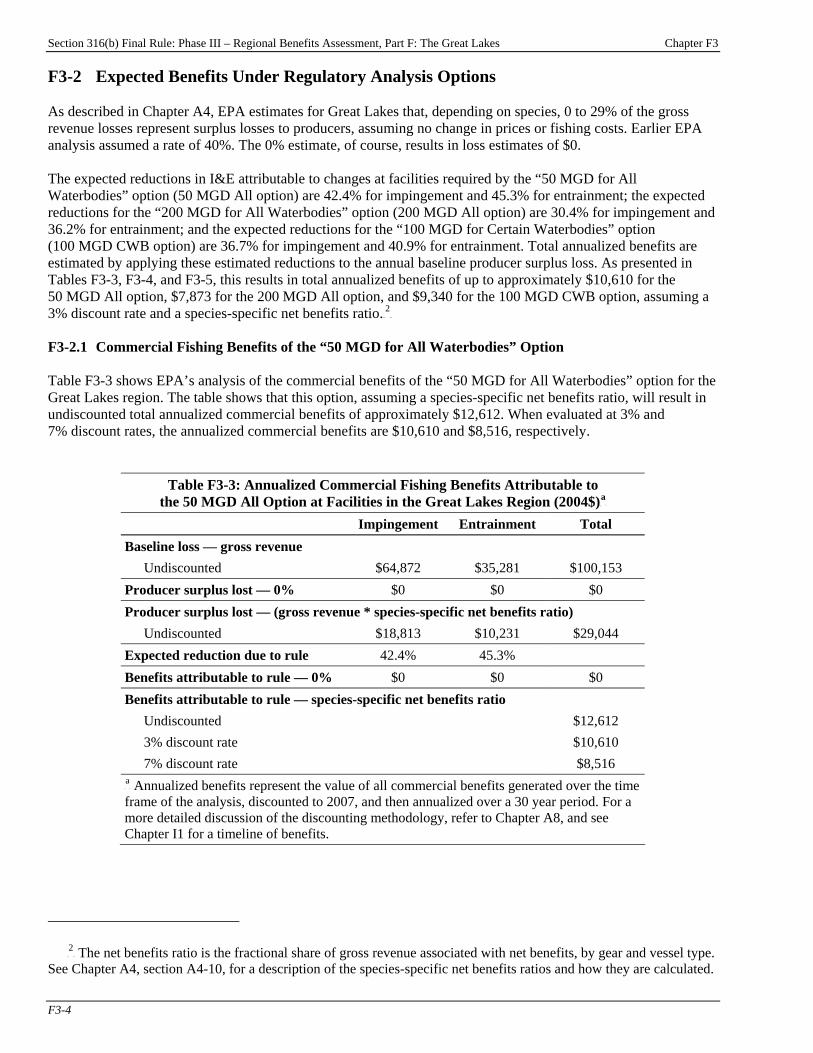
Section 316(b) Final Rule: Phase III – Regional Benefits Assessment, Part F: The Great Lakes Chapter F3
F3-4
F3-2 Expected Benefits Under Regulatory Analysis Options As described in Chapter A4, EPA estimates for Great Lakes that, depending on species, 0 to 29% of the gross revenue losses represent surplus losses to producers, assuming no change in prices or fishing costs. Earlier EPA analysis assumed a rate of 40%. The 0% estimate, of course, results in loss estimates of $0. The expected reductions in I&E attributable to changes at facilities required by the “50 MGD for All Waterbodies” option (50 MGD All option) are 42.4% for impingement and 45.3% for entrainment; the expected reductions for the “200 MGD for All Waterbodies” option (200 MGD All option) are 30.4% for impingement and 36.2% for entrainment; and the expected reductions for the “100 MGD for Certain Waterbodies” option (100 MGD CWB option) are 36.7% for impingement and 40.9% for entrainment. Total annualized benefits are estimated by applying these estimated reductions to the annual baseline producer surplus loss. As presented in Tables F3-3, F3-4, and F3-5, this results in total annualized benefits of up to approximately $10,610 for the 50 MGD All option, $7,873 for the 200 MGD All option, and $9,340 for the 100 MGD CWB option, assuming a 3% discount rate and a species-specific net benefits ratio.TPF
2FPT
F3-2.1 Commercial Fishing Benefits of the “50 MGD for All Waterbodies” Option Table F3-3 shows EPA’s analysis of the commercial benefits of the “50 MGD for All Waterbodies” option for the Great Lakes region. The table shows that this option, assuming a species-specific net benefits ratio, will result in undiscounted total annualized commercial benefits of approximately $12,612. When evaluated at 3% and 7% discount rates, the annualized commercial benefits are $10,610 and $8,516, respectively.
Table F3-3: Annualized Commercial Fishing Benefits Attributable to the 50 MGD All Option at Facilities in the Great Lakes Region (2004$)P
aP
Impingement Entrainment Total Baseline loss — gross revenue
Undiscounted $64,872 $35,281 $100,153 Producer surplus lost — 0% $0 $0 $0 Producer surplus lost — (gross revenue * species-specific net benefits ratio)
Undiscounted $18,813 $10,231 $29,044 Expected reduction due to rule 42.4% 45.3% Benefits attributable to rule — 0% $0 $0 $0 Benefits attributable to rule — species-specific net benefits ratio
Undiscounted $12,612 3% discount rate $10,610 7% discount rate $8,516
P
aP Annualized benefits represent the value of all commercial benefits generated over the time
frame of the analysis, discounted to 2007, and then annualized over a 30 year period. For a more detailed discussion of the discounting methodology, refer to Chapter A8, and see Chapter I1 for a timeline of benefits.
TP
2PT The net benefits ratio is the fractional share of gross revenue associated with net benefits, by gear and vessel type.
See Chapter A4, section A4-10, for a description of the species-specific net benefits ratios and how they are calculated.
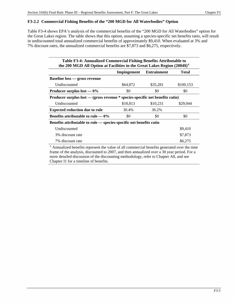
Section 316(b) Final Rule: Phase III – Regional Benefits Assessment, Part F: The Great Lakes Chapter F3
F3-5
F3-2.2 Commercial Fishing Benefits of the “200 MGD for All Waterbodies” Option Table F3-4 shows EPA’s analysis of the commercial benefits of the “200 MGD for All Waterbodies” option for the Great Lakes region. The table shows that this option, assuming a species-specific net benefits ratio, will result in undiscounted total annualized commercial benefits of approximately $9,410. When evaluated at 3% and 7% discount rates, the annualized commercial benefits are $7,873 and $6,275, respectively.
Table F3-4: Annualized Commercial Fishing Benefits Attributable to the 200 MGD All Option at Facilities in the Great Lakes Region (2004$)P
aP
Impingement Entrainment Total Baseline loss — gross revenue
Undiscounted $64,872 $35,281 $100,153 Producer surplus lost — 0% $0 $0 $0 Producer surplus lost — (gross revenue * species-specific net benefits ratio)
Undiscounted $18,813 $10,231 $29,044 Expected reduction due to rule 30.4% 36.2% Benefits attributable to rule — 0% $0 $0 $0 Benefits attributable to rule — species-specific net benefits ratio
Undiscounted $9,410 3% discount rate $7,873 7% discount rate $6,275
P
aP Annualized benefits represent the value of all commercial benefits generated over the time
frame of the analysis, discounted to 2007, and then annualized over a 30 year period. For a more detailed discussion of the discounting methodology, refer to Chapter A8, and see Chapter I1 for a timeline of benefits.
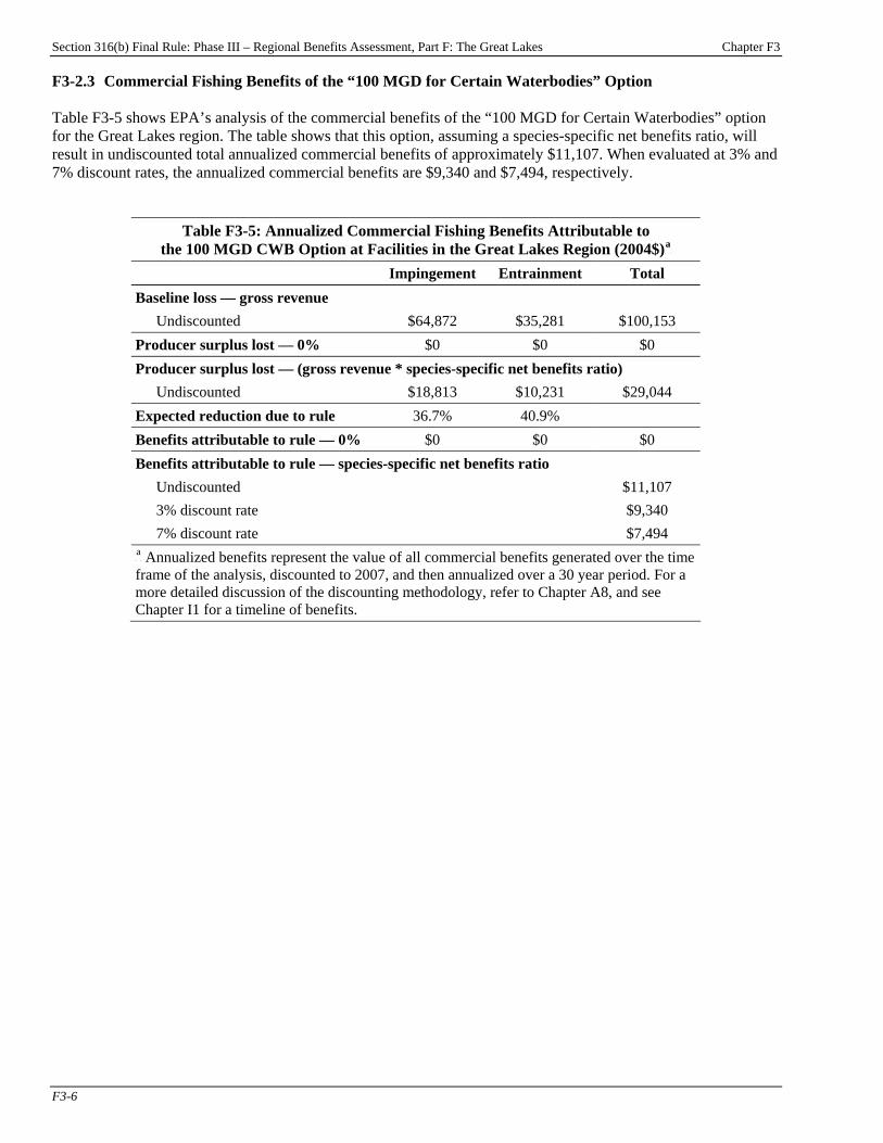
Section 316(b) Final Rule: Phase III – Regional Benefits Assessment, Part F: The Great Lakes Chapter F3
F3-6
F3-2.3 Commercial Fishing Benefits of the “100 MGD for Certain Waterbodies” Option Table F3-5 shows EPA’s analysis of the commercial benefits of the “100 MGD for Certain Waterbodies” option for the Great Lakes region. The table shows that this option, assuming a species-specific net benefits ratio, will result in undiscounted total annualized commercial benefits of approximately $11,107. When evaluated at 3% and 7% discount rates, the annualized commercial benefits are $9,340 and $7,494, respectively.
Table F3-5: Annualized Commercial Fishing Benefits Attributable to the 100 MGD CWB Option at Facilities in the Great Lakes Region (2004$)P
aP
Impingement Entrainment Total Baseline loss — gross revenue
Undiscounted $64,872 $35,281 $100,153 Producer surplus lost — 0% $0 $0 $0 Producer surplus lost — (gross revenue * species-specific net benefits ratio)
Undiscounted $18,813 $10,231 $29,044 Expected reduction due to rule 36.7% 40.9% Benefits attributable to rule — 0% $0 $0 $0 Benefits attributable to rule — species-specific net benefits ratio
Undiscounted $11,107 3% discount rate $9,340 7% discount rate $7,494
P
aP Annualized benefits represent the value of all commercial benefits generated over the time
frame of the analysis, discounted to 2007, and then annualized over a 30 year period. For a more detailed discussion of the discounting methodology, refer to Chapter A8, and see Chapter I1 for a timeline of benefits.

Section 316(b) Final Rule: Phase III – Regional Benefits Assessment, Part F: The Great Lakes Appendix F3
App. F3-1
Appendix F3: Commercial Fishing Benefits Under Supplemental Policy Options
Introduction Chapter F3 presents EPA’s estimates of the commercial benefits of the regulatory options for the section 316(b) rule for Phase III facilities in the Great Lakes region. To facilitate comparisons among the options, this appendix presents estimates of the commercial fishing benefits of several supplemental options that EPA evaluated in preparation for this rule:
Appendix Contents F3-1 Commercial Fishing Benefits of the Supplemental Options .................................F3-2
< “Electric Generators 2-50 MGD I-only Everywhere” option; < “Electric Generators 2-50 MGD I&E like Phase II” option; < “Electric Generators 2-50 MGD I&E Everywhere” option; < “Manufacturers 2-50 MGD I-only Everywhere” option; < “Manufacturers 2-50 MGD I&E like Phase II” option; < “Manufacturers 2-50 MGD I&E Everywhere” option; < “Manufacturers 50+ MGD I-only Everywhere” option; and < “Manufacturers 50+ MGD I&E Everywhere” option.
Commercial fishing benefits presented in this chapter were estimated using the benefit transfer approach discussed in Chapter F3 and in Chapter A4, “Methods for Estimating Commercial Fishing Benefits.” For more information on the options, please see the TDD.
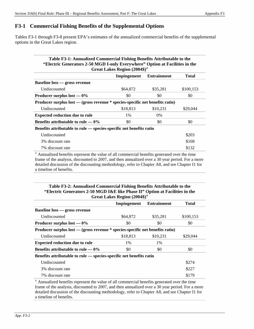
Section 316(b) Final Rule: Phase III – Regional Benefits Assessment, Part F: The Great Lakes Appendix F3
App. F3-2
F3-1 Commercial Fishing Benefits of the Supplemental Options Tables F3-1 through F3-8 present EPA’s estimates of the annualized commercial benefits of the supplemental options in the Great Lakes region.
Table F3-1: Annualized Commercial Fishing Benefits Attributable to the “Electric Generators 2-50 MGD I-only Everywhere” Option at Facilities in the
Great Lakes Region (2004$)P
aP
Impingement Entrainment Total Baseline loss — gross revenue
Undiscounted $64,872 $35,281 $100,153 Producer surplus lost — 0% $0 $0 $0 Producer surplus lost — (gross revenue * species-specific net benefits ratio)
Undiscounted $18,813 $10,231 $29,044 Expected reduction due to rule 1% 0% Benefits attributable to rule — 0% $0 $0 $0 Benefits attributable to rule — species-specific net benefits ratio
Undiscounted $203 3% discount rate $168 7% discount rate $132
P
aP Annualized benefits represent the value of all commercial benefits generated over the time
frame of the analysis, discounted to 2007, and then annualized over a 30 year period. For a more detailed discussion of the discounting methodology, refer to Chapter A8, and see Chapter I1 for a timeline of benefits.
Table F3-2: Annualized Commercial Fishing Benefits Attributable to the “Electric Generators 2-50 MGD I&E like Phase II” Option at Facilities in the
Great Lakes Region (2004$)P
aP
Impingement Entrainment Total Baseline loss — gross revenue
Undiscounted $64,872 $35,281 $100,153 Producer surplus lost — 0% $0 $0 $0 Producer surplus lost — (gross revenue * species-specific net benefits ratio)
Undiscounted $18,813 $10,231 $29,044 Expected reduction due to rule 1% 1% Benefits attributable to rule — 0% $0 $0 $0 Benefits attributable to rule — species-specific net benefits ratio
Undiscounted $274 3% discount rate $227 7% discount rate $179
P
aP Annualized benefits represent the value of all commercial benefits generated over the time
frame of the analysis, discounted to 2007, and then annualized over a 30 year period. For a more detailed discussion of the discounting methodology, refer to Chapter A8, and see Chapter I1 for a timeline of benefits.
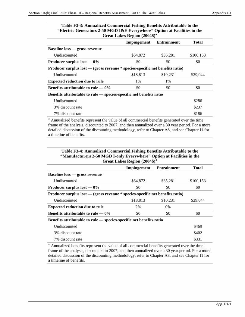
Section 316(b) Final Rule: Phase III – Regional Benefits Assessment, Part F: The Great Lakes Appendix F3
App. F3-3
Table F3-3: Annualized Commercial Fishing Benefits Attributable to the “Electric Generators 2-50 MGD I&E Everywhere” Option at Facilities in the
Great Lakes Region (2004$)P
aP
Impingement Entrainment Total Baseline loss — gross revenue
Undiscounted $64,872 $35,281 $100,153 Producer surplus lost — 0% $0 $0 $0 Producer surplus lost — (gross revenue * species-specific net benefits ratio)
Undiscounted $18,813 $10,231 $29,044 Expected reduction due to rule 1% 1% Benefits attributable to rule — 0% $0 $0 $0 Benefits attributable to rule — species-specific net benefits ratio
Undiscounted $286 3% discount rate $237 7% discount rate $186
P
aP Annualized benefits represent the value of all commercial benefits generated over the time
frame of the analysis, discounted to 2007, and then annualized over a 30 year period. For a more detailed discussion of the discounting methodology, refer to Chapter A8, and see Chapter I1 for a timeline of benefits.
Table F3-4: Annualized Commercial Fishing Benefits Attributable to the “Manufacturers 2-50 MGD I-only Everywhere” Option at Facilities in the
Great Lakes Region (2004$)P
aP
Impingement Entrainment Total Baseline loss — gross revenue
Undiscounted $64,872 $35,281 $100,153 Producer surplus lost — 0% $0 $0 $0 Producer surplus lost — (gross revenue * species-specific net benefits ratio)
Undiscounted $18,813 $10,231 $29,044 Expected reduction due to rule 2% 0% Benefits attributable to rule — 0% $0 $0 $0 Benefits attributable to rule — species-specific net benefits ratio
Undiscounted $469 3% discount rate $402 7% discount rate $331
P
aP Annualized benefits represent the value of all commercial benefits generated over the time
frame of the analysis, discounted to 2007, and then annualized over a 30 year period. For a more detailed discussion of the discounting methodology, refer to Chapter A8, and see Chapter I1 for a timeline of benefits.
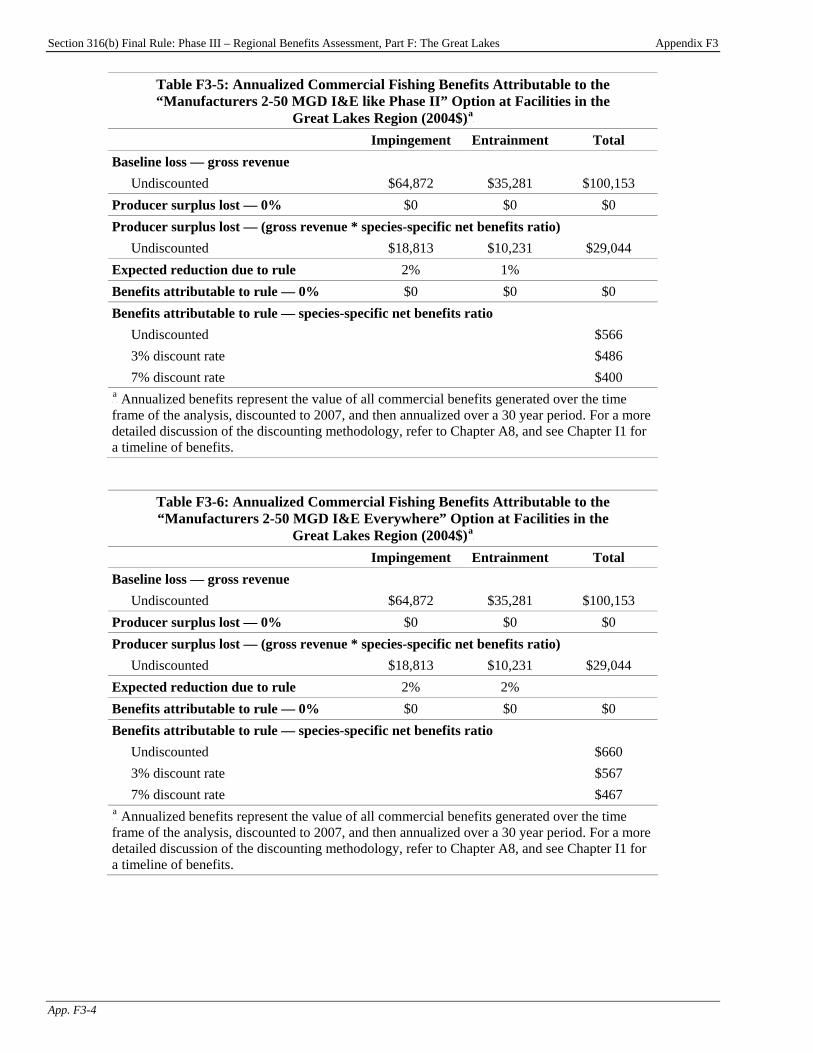
Section 316(b) Final Rule: Phase III – Regional Benefits Assessment, Part F: The Great Lakes Appendix F3
App. F3-4
Table F3-5: Annualized Commercial Fishing Benefits Attributable to the “Manufacturers 2-50 MGD I&E like Phase II” Option at Facilities in the
Great Lakes Region (2004$)P
aP
Impingement Entrainment Total Baseline loss — gross revenue
Undiscounted $64,872 $35,281 $100,153 Producer surplus lost — 0% $0 $0 $0 Producer surplus lost — (gross revenue * species-specific net benefits ratio)
Undiscounted $18,813 $10,231 $29,044 Expected reduction due to rule 2% 1% Benefits attributable to rule — 0% $0 $0 $0 Benefits attributable to rule — species-specific net benefits ratio
Undiscounted $566 3% discount rate $486 7% discount rate $400
P
aP Annualized benefits represent the value of all commercial benefits generated over the time
frame of the analysis, discounted to 2007, and then annualized over a 30 year period. For a more detailed discussion of the discounting methodology, refer to Chapter A8, and see Chapter I1 for a timeline of benefits.
Table F3-6: Annualized Commercial Fishing Benefits Attributable to the “Manufacturers 2-50 MGD I&E Everywhere” Option at Facilities in the
Great Lakes Region (2004$)P
aP
Impingement Entrainment Total Baseline loss — gross revenue
Undiscounted $64,872 $35,281 $100,153 Producer surplus lost — 0% $0 $0 $0 Producer surplus lost — (gross revenue * species-specific net benefits ratio)
Undiscounted $18,813 $10,231 $29,044 Expected reduction due to rule 2% 2% Benefits attributable to rule — 0% $0 $0 $0 Benefits attributable to rule — species-specific net benefits ratio
Undiscounted $660 3% discount rate $567 7% discount rate $467
P
aP Annualized benefits represent the value of all commercial benefits generated over the time
frame of the analysis, discounted to 2007, and then annualized over a 30 year period. For a more detailed discussion of the discounting methodology, refer to Chapter A8, and see Chapter I1 for a timeline of benefits.

Section 316(b) Final Rule: Phase III – Regional Benefits Assessment, Part F: The Great Lakes Appendix F3
App. F3-5
Table F3-7: Annualized Commercial Fishing Benefits Attributable to the “Manufacturers 50+ MGD I-only Everywhere” Option at Facilities in the
Great Lakes Region (2004$)P
aP
Impingement Entrainment Total Baseline loss — gross revenue
Undiscounted $64,872 $35,281 $100,153 Producer surplus lost — 0% $0 $0 $0 Producer surplus lost — (gross revenue * species-specific net benefits ratio)
Undiscounted $18,813 $10,231 $29,044 Expected reduction due to rule 42% 0% Benefits attributable to rule — 0% $0 $0 $0 Benefits attributable to rule — species-specific net benefits ratio
Undiscounted $7,882 3% discount rate $6,561 7% discount rate $5,196
P
aP Annualized benefits represent the value of all commercial benefits generated over the time
frame of the analysis, discounted to 2007, and then annualized over a 30 year period. For a more detailed discussion of the discounting methodology, refer to Chapter A8, and see Chapter I1 for a timeline of benefits.
Table F3-8: Annualized Commercial Fishing Benefits Attributable to the “Manufacturers 50+ MGD I&E Everywhere” Option at Facilities in the
Great Lakes Region (2004$)P
aP
Impingement Entrainment Total Baseline loss — gross revenue
Undiscounted $64,872 $35,281 $100,153 Producer surplus lost — 0% $0 $0 $0 Producer surplus lost — (gross revenue * species-specific net benefits ratio)
Undiscounted $18,813 $10,231 $29,044 Expected reduction due to rule 42% 46% Benefits attributable to rule — 0% $0 $0 $0 Benefits attributable to rule — species-specific net benefits ratio
Undiscounted $12,580 3% discount rate $10,583 7% discount rate $8,494
P
aP Annualized benefits represent the value of all commercial benefits generated over the time
frame of the analysis, discounted to 2007, and then annualized over a 30 year period. For a more detailed discussion of the discounting methodology, refer to Chapter A8, and see Chapter I1 for a timeline of benefits.
Section 316(b) Final Rule: Phase III – Regional Benefits Assessment, Part F: The Great Lakes Chapter F4
F4-1
Chapter F4: Recreational Use Benefits Introduction
Chapter Contents F4-1 Benefit Transfer Approach Based on Meta- Analysis ......................................................... F4-1 F4-1.1 Baseline Losses and Reductions in Recreational Fishery Losses Under the Regulatory Options................... F4-2 F4-1.2 Recreational Fishing Benefits from Eliminating Baseline I&E Losses............................................... F4-3 F4-1.3 Recreational Fishing Benefits of the “50 MGD for All Waterbodies” Option .............................................. F4-4 F4-1.4 Recreational Fishing Benefits of the “200 MGD for All Waterbodies” Option .............................................. F4-5 F4-1.5 Recreational Fishing Benefits of the “100 MGD for Certain Waterbodies” Option .............................................. F4-6 F4-2 Limitations and Uncertainty .......................... F4-7
This chapter presents the results of the recreational fishing benefits analysis for the Great Lakes region. The chapter presents EPA’s estimates of baseline (i.e., current) annual recreational fishery losses from impingement and entrainment (I&E) at potentially regulated facilities in the Great Lakes region and annual reductions in these losses under the regulatory options for Phase III existing facilitiesTPF
1FPT:
< the “50 MGD for All Waterbodies” option, < the “200 MGD for All Waterbodies” option,
and < the “100 MGD for Certain Waterbodies”
option. The chapter then presents the estimated welfare gain to Great Lakes anglers from eliminating baseline recreational fishing losses from I&E and the expected benefits under the regulatory options. EPA estimated the recreational benefits of reducing and eliminating I&E losses using a benefit transfer methodology based on a meta-analysis of the marginal value of catching different species of fish. This meta-analysis is discussed in detail in Chapter A5, “Recreational Fishing Benefits Methodology.” EPA considered a wide range of policy options in developing this regulation. In addition to the regulatory options, EPA evaluated several supplemental options. Appendix F4 presents results of the recreational fishing benefits analysis for the supplemental options. For additional information on the options, please see the TDD. F4-1 Benefit Transfer Approach Based on Meta-Analysis EPA estimated the recreational welfare gain from the reduction in annual I&E losses expected under the policy options, and the welfare gain from eliminating I&E at potentially regulated facilities, using a benefit transfer approach. As discussed in Chapter A5, the Agency used a meta-analysis regression equation to estimate the marginal recreational value per additional fish caught by anglers, for different species in different regions. Since I&E at potentially regulated facilities affects a variety of species, EPA assigned each species with I&E losses to one of the general species groups used in the meta-analysis. The Agency then calculated the economic value of reducing or eliminating baseline I&E losses, for each species group, by multiplying the value per fish for that species group by the number of fish in the group that are lost in the baseline or saved under the policy options.TPF
2FPT
P
1P See the Introduction to this report for a description of the primary analysis options.
TP
2PT The estimates of I&E presented in this chapter include only the fraction of impinged and entrained recreational
fish that would be caught by anglers. The total amount of I&E of recreational species is actually much higher.

Section 316(b) Final Rule: Phase III – Regional Benefits Assessment, Part F: The Great Lakes Chapter F4
F4-2
In general, the fit between the species with I&E losses and the species groups in the meta-analysis was good. However, EPA’s estimates of baseline I&E losses and reductions in I&E under the policy options included losses of “unidentified” species. The “unidentified” group includes fish lost indirectly through trophic transfer, as well as species for which no species information was available.TPF
3FPT Rather than using the meta-analysis regression to try to
predict the value per fish for an “unidentified” species, EPA assumed that per-fish values for these species can be approximated by the weighted average value per fish for all species affected by I&E in the Great Lakes region.TPF
4FPT
F4-1.1 Baseline Losses and Reductions in Recreational Fishery Losses Under the Regulatory Options Table F4-1 presents EPA’s estimates of baseline (i.e., current) annual recreational I&E losses at potentially regulated facilities and annual reductions in these losses under each of the regulatory options, in the Great Lakes region. The table shows that total baseline losses to recreational fisheries are 225.5 thousand fish per year. In comparison, the “50 MGD for All Waterbodies” option prevents losses of 96.7 thousand fish per year, the “200 MGD for All Waterbodies” option prevents losses of 72.1 thousand fish per year, and the “100 MGD for Certain Waterbodies” option prevents losses of 85.1 thousand fish per year. Of all the affected species, white bass and “unidentified” species have the highest losses in the baseline and the highest prevented losses under the regulatory options.
TP
3PT In addition to recreational fish that are lost because they are impinged or entrained, some recreational fish are lost
because the forage fish that they feed on are impinged or entrained, and thus removed from the food chain. These trophic transfer losses of recreational species are included in EPA’s estimates of total I&E losses. Since it is difficult to predict which recreational species would be affected by losses of forage fish, these losses are classified as “unidentified” recreational species. Also included in the “unidentified” group are losses of fish that were reported by facilities without information about their exact species.
TP
4PT EPA used the estimated level of baseline recreational losses for each species group as a weighting factor.
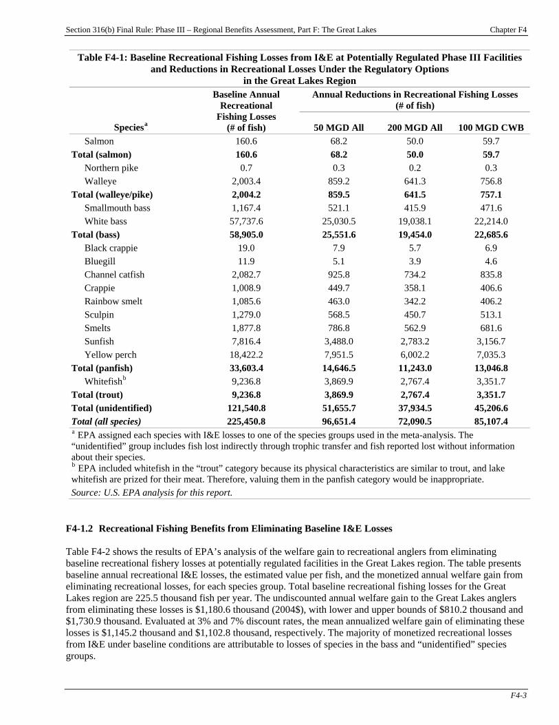
Section 316(b) Final Rule: Phase III – Regional Benefits Assessment, Part F: The Great Lakes Chapter F4
F4-3
Table F4-1: Baseline Recreational Fishing Losses from I&E at Potentially Regulated Phase III Facilities and Reductions in Recreational Losses Under the Regulatory Options
in the Great Lakes Region Annual Reductions in Recreational Fishing Losses
(# of fish)
SpeciesP
aP
Baseline Annual Recreational
Fishing Losses (# of fish) 50 MGD All 200 MGD All 100 MGD CWB
Salmon 160.6 68.2 50.0 59.7 Total (salmon) 160.6 68.2 50.0 59.7
Northern pike 0.7 0.3 0.2 0.3 Walleye 2,003.4 859.2 641.3 756.8
Total (walleye/pike) 2,004.2 859.5 641.5 757.1 Smallmouth bass 1,167.4 521.1 415.9 471.6 White bass 57,737.6 25,030.5 19,038.1 22,214.0
Total (bass) 58,905.0 25,551.6 19,454.0 22,685.6 Black crappie 19.0 7.9 5.7 6.9 Bluegill 11.9 5.1 3.9 4.6 Channel catfish 2,082.7 925.8 734.2 835.8 Crappie 1,008.9 449.7 358.1 406.6 Rainbow smelt 1,085.6 463.0 342.2 406.2 Sculpin 1,279.0 568.5 450.7 513.1 Smelts 1,877.8 786.8 562.9 681.6 Sunfish 7,816.4 3,488.0 2,783.2 3,156.7 Yellow perch 18,422.2 7,951.5 6,002.2 7,035.3
Total (panfish) 33,603.4 14,646.5 11,243.0 13,046.8 WhitefishP
bP 9,236.8 3,869.9 2,767.4 3,351.7
Total (trout) 9,236.8 3,869.9 2,767.4 3,351.7 Total (unidentified) 121,540.8 51,655.7 37,934.5 45,206.6 Total (all species) 225,450.8 96,651.4 72,090.5 85,107.4 P
aP EPA assigned each species with I&E losses to one of the species groups used in the meta-analysis. The
“unidentified” group includes fish lost indirectly through trophic transfer and fish reported lost without information about their species. P
bP EPA included whitefish in the “trout” category because its physical characteristics are similar to trout, and lake
whitefish are prized for their meat. Therefore, valuing them in the panfish category would be inappropriate. Source: U.S. EPA analysis for this report.
F4-1.2 Recreational Fishing Benefits from Eliminating Baseline I&E Losses Table F4-2 shows the results of EPA’s analysis of the welfare gain to recreational anglers from eliminating baseline recreational fishery losses at potentially regulated facilities in the Great Lakes region. The table presents baseline annual recreational I&E losses, the estimated value per fish, and the monetized annual welfare gain from eliminating recreational losses, for each species group. Total baseline recreational fishing losses for the Great Lakes region are 225.5 thousand fish per year. The undiscounted annual welfare gain to the Great Lakes anglers from eliminating these losses is $1,180.6 thousand (2004$), with lower and upper bounds of $810.2 thousand and $1,730.9 thousand. Evaluated at 3% and 7% discount rates, the mean annualized welfare gain of eliminating these losses is $1,145.2 thousand and $1,102.8 thousand, respectively. The majority of monetized recreational losses from I&E under baseline conditions are attributable to losses of species in the bass and “unidentified” species groups.

Section 316(b) Final Rule: Phase III – Regional Benefits Assessment, Part F: The Great Lakes Chapter F4
F4-4
Table F4-2: Recreational Fishing Benefits from Eliminating Baseline I&E at Potentially Regulated Phase III Facilities in the Great Lakes Region (2004$)
Value per FishP
bP
Annualized Benefits from Eliminating Recreational Fishing
Losses (thousands)P
c,dP
Species Group
Baseline Annual Recreational
Fishing Losses (thousands of fish)P
aP Low Mean High Low Mean High
Salmon 0.2 $8.42 $11.17 $14.83 $1.4 $1.8 $2.4 Trout 9.2 $5.87 $7.94 $10.79 $54.2 $73.4 $99.7 Walleye/pike 2.0 $2.12 $3.46 $5.69 $4.3 $6.9 $11.4 Bass 58.9 $4.90 $7.21 $10.64 $288.8 $424.5 $626.5 Panfish 33.6 $0.74 $1.12 $1.72 $24.8 $37.5 $57.8 Unidentified 121.5 $3.59 $5.24 $7.68 $436.8 $636.5 $933.1 Total (undiscounted) 225.5 $810.2 $1,180.6 $1,730.9 Total (evaluated at 3% discount rate) 225.5 $785.9 $1,145.2 $1,678.9 Total (evaluated at 7% discount rate) 225.5 $756.8 $1,102.8 $1,616.7 P
aP Recreational fishing losses include only the portion of impinged and entrained fish that would have been caught by
recreational anglers. P
bP Lower and upper bounds on per-fish values are based on the 5% and 95% confidence bounds predicted by the
Krinsky and Robb approach. See section A5-5.1 of Chapter A5 for more details on this approach. P
cP Monetized benefits are calculated by multiplying baseline losses by the estimated value per fish.
P
dP Annualized values represent the total welfare gain over the time frame of the analysis from eliminating recreational
losses, discounted to 2007, and then annualized over a thirty year period. For a detailed discussion of the discounting and annualization methodology, refer to Chapter A8. Source: U.S. EPA analysis for this report.
F4-1.3 Recreational Fishing Benefits of the “50 MGD for All Waterbodies” Option Table F4-3 shows the results of EPA’s analysis of the recreational benefits of the “50 MGD for All Waterbodies” option for the Great Lakes region. The table presents the annual reduction in recreational I&E losses expected under this option, the estimated value per fish, and annual monetized recreational welfare gain from this option, by species group. The table shows that this option reduces recreational losses by 96.7 thousand fish per year, resulting in an undiscounted welfare gain to recreational anglers of $505.5 thousand (2004$), with lower and upper bounds of $346.8 thousand and $741.2 thousand. Evaluated at 3% and 7% discount rates, the mean annualized welfare gain from this reduction in recreational losses is $425.3 thousand and $341.3 thousand, respectively. The majority of benefits result from reduced losses of species in the bass and “unidentified” species groups.
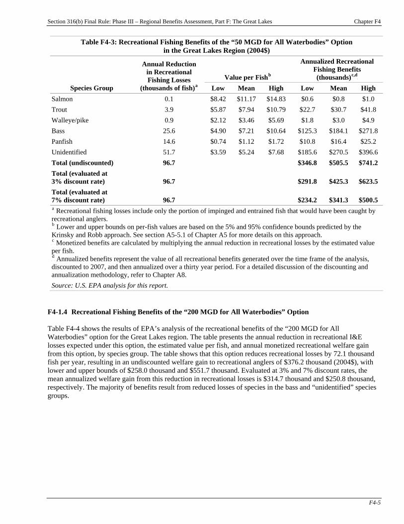
Section 316(b) Final Rule: Phase III – Regional Benefits Assessment, Part F: The Great Lakes Chapter F4
F4-5
Table F4-3: Recreational Fishing Benefits of the “50 MGD for All Waterbodies” Option in the Great Lakes Region (2004$)
Value per FishP
bP
Annualized Recreational Fishing Benefits (thousands)P
c,dP
Species Group
Annual Reduction in Recreational Fishing Losses
(thousands of fish)P
aP Low Mean High Low Mean High
Salmon 0.1 $8.42 $11.17 $14.83 $0.6 $0.8 $1.0 Trout 3.9 $5.87 $7.94 $10.79 $22.7 $30.7 $41.8 Walleye/pike 0.9 $2.12 $3.46 $5.69 $1.8 $3.0 $4.9 Bass 25.6 $4.90 $7.21 $10.64 $125.3 $184.1 $271.8 Panfish 14.6 $0.74 $1.12 $1.72 $10.8 $16.4 $25.2 Unidentified 51.7 $3.59 $5.24 $7.68 $185.6 $270.5 $396.6 Total (undiscounted) 96.7 $346.8 $505.5 $741.2 Total (evaluated at 3% discount rate) 96.7 $291.8 $425.3 $623.5 Total (evaluated at 7% discount rate) 96.7 $234.2 $341.3 $500.5 P
aP Recreational fishing losses include only the portion of impinged and entrained fish that would have been caught by
recreational anglers. P
bP Lower and upper bounds on per-fish values are based on the 5% and 95% confidence bounds predicted by the
Krinsky and Robb approach. See section A5-5.1 of Chapter A5 for more details on this approach. P
cP Monetized benefits are calculated by multiplying the annual reduction in recreational losses by the estimated value
per fish. P
dP Annualized benefits represent the value of all recreational benefits generated over the time frame of the analysis,
discounted to 2007, and then annualized over a thirty year period. For a detailed discussion of the discounting and annualization methodology, refer to Chapter A8. Source: U.S. EPA analysis for this report.
F4-1.4 Recreational Fishing Benefits of the “200 MGD for All Waterbodies” Option Table F4-4 shows the results of EPA’s analysis of the recreational benefits of the “200 MGD for All Waterbodies” option for the Great Lakes region. The table presents the annual reduction in recreational I&E losses expected under this option, the estimated value per fish, and annual monetized recreational welfare gain from this option, by species group. The table shows that this option reduces recreational losses by 72.1 thousand fish per year, resulting in an undiscounted welfare gain to recreational anglers of $376.2 thousand (2004$), with lower and upper bounds of $258.0 thousand and $551.7 thousand. Evaluated at 3% and 7% discount rates, the mean annualized welfare gain from this reduction in recreational losses is $314.7 thousand and $250.8 thousand, respectively. The majority of benefits result from reduced losses of species in the bass and “unidentified” species groups.
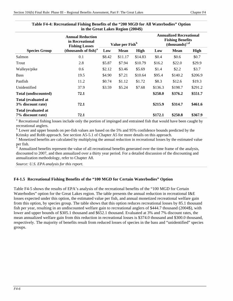
Section 316(b) Final Rule: Phase III – Regional Benefits Assessment, Part F: The Great Lakes Chapter F4
F4-6
Table F4-4: Recreational Fishing Benefits of the “200 MGD for All Waterbodies” Option in the Great Lakes Region (2004$)
Value per FishP
bP
Annualized Recreational Fishing Benefits (thousands)P
c,dP
Species Group
Annual Reduction in Recreational Fishing Losses
(thousands of fish)P
aP Low Mean High Low Mean High
Salmon 0.1 $8.42 $11.17 $14.83 $0.4 $0.6 $0.7 Trout 2.8 $5.87 $7.94 $10.79 $16.2 $22.0 $29.9 Walleye/pike 0.6 $2.12 $3.46 $5.69 $1.4 $2.2 $3.7 Bass 19.5 $4.90 $7.21 $10.64 $95.4 $140.2 $206.9 Panfish 11.2 $0.74 $1.12 $1.72 $8.3 $12.6 $19.3 Unidentified 37.9 $3.59 $5.24 $7.68 $136.3 $198.7 $291.2 Total (undiscounted) 72.1 $258.0 $376.2 $551.7 Total (evaluated at 3% discount rate) 72.1 $215.9 $314.7 $461.6 Total (evaluated at 7% discount rate) 72.1 $172.1 $250.8 $367.9 P
aP Recreational fishing losses include only the portion of impinged and entrained fish that would have been caught by
recreational anglers. P
bP Lower and upper bounds on per-fish values are based on the 5% and 95% confidence bounds predicted by the
Krinsky and Robb approach. See section A5-5.1 of Chapter A5 for more details on this approach. P
cP Monetized benefits are calculated by multiplying the annual reduction in recreational losses by the estimated value
per fish. P
dP Annualized benefits represent the value of all recreational benefits generated over the time frame of the analysis,
discounted to 2007, and then annualized over a thirty year period. For a detailed discussion of the discounting and annualization methodology, refer to Chapter A8. Source: U.S. EPA analysis for this report.
F4-1.5 Recreational Fishing Benefits of the “100 MGD for Certain Waterbodies” Option Table F4-5 shows the results of EPA’s analysis of the recreational benefits of the “100 MGD for Certain Waterbodies” option for the Great Lakes region. The table presents the annual reduction in recreational I&E losses expected under this option, the estimated value per fish, and annual monetized recreational welfare gain from this option, by species group. The table shows that this option reduces recreational losses by 85.1 thousand fish per year, resulting in an undiscounted welfare gain to recreational anglers of $444.7 thousand (2004$), with lower and upper bounds of $305.1 thousand and $652.1 thousand. Evaluated at 3% and 7% discount rates, the mean annualized welfare gain from this reduction in recreational losses is $374.0 thousand and $300.0 thousand, respectively. The majority of benefits result from reduced losses of species in the bass and “unidentified” species groups.
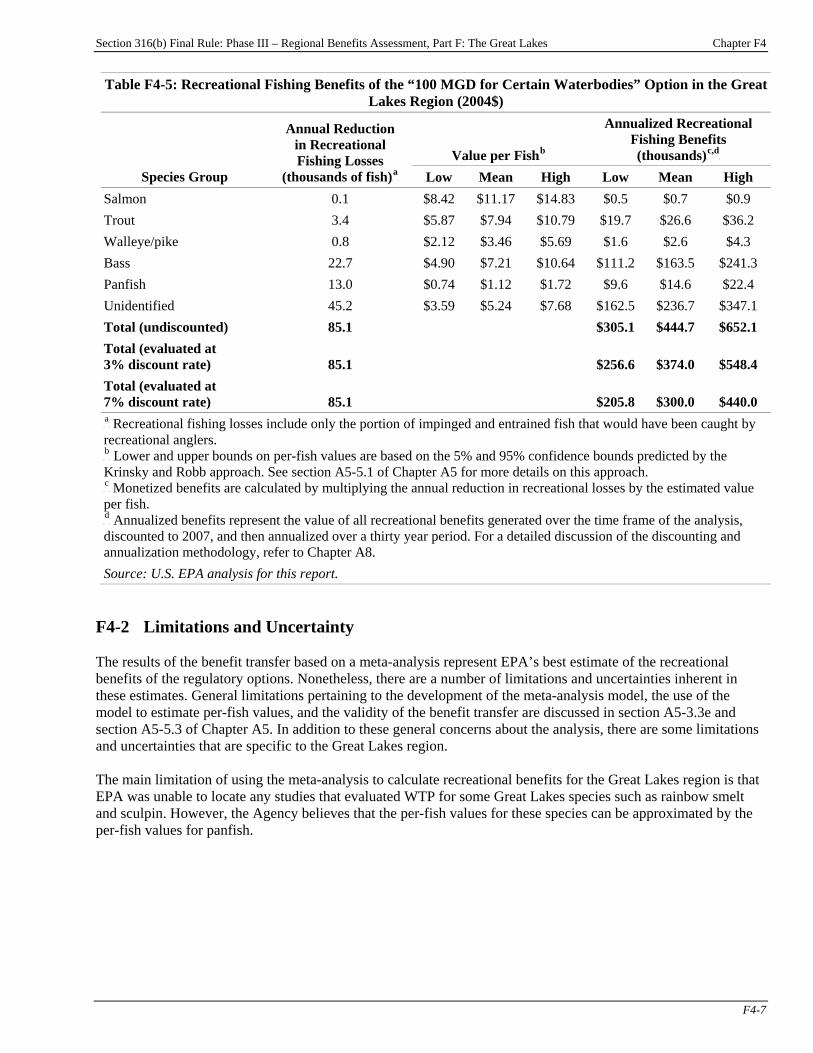
Section 316(b) Final Rule: Phase III – Regional Benefits Assessment, Part F: The Great Lakes Chapter F4
F4-7
Table F4-5: Recreational Fishing Benefits of the “100 MGD for Certain Waterbodies” Option in the Great Lakes Region (2004$)
Value per FishP
bP
Annualized Recreational Fishing Benefits (thousands)P
c,dP
Species Group
Annual Reduction in Recreational Fishing Losses
(thousands of fish)P
aP Low Mean High Low Mean High
Salmon 0.1 $8.42 $11.17 $14.83 $0.5 $0.7 $0.9 Trout 3.4 $5.87 $7.94 $10.79 $19.7 $26.6 $36.2 Walleye/pike 0.8 $2.12 $3.46 $5.69 $1.6 $2.6 $4.3 Bass 22.7 $4.90 $7.21 $10.64 $111.2 $163.5 $241.3 Panfish 13.0 $0.74 $1.12 $1.72 $9.6 $14.6 $22.4 Unidentified 45.2 $3.59 $5.24 $7.68 $162.5 $236.7 $347.1 Total (undiscounted) 85.1 $305.1 $444.7 $652.1 Total (evaluated at 3% discount rate) 85.1 $256.6 $374.0 $548.4 Total (evaluated at 7% discount rate) 85.1 $205.8 $300.0 $440.0 P
aP Recreational fishing losses include only the portion of impinged and entrained fish that would have been caught by
recreational anglers. P
bP Lower and upper bounds on per-fish values are based on the 5% and 95% confidence bounds predicted by the
Krinsky and Robb approach. See section A5-5.1 of Chapter A5 for more details on this approach. P
cP Monetized benefits are calculated by multiplying the annual reduction in recreational losses by the estimated value
per fish. P
dP Annualized benefits represent the value of all recreational benefits generated over the time frame of the analysis,
discounted to 2007, and then annualized over a thirty year period. For a detailed discussion of the discounting and annualization methodology, refer to Chapter A8. Source: U.S. EPA analysis for this report.
F4-2 Limitations and Uncertainty The results of the benefit transfer based on a meta-analysis represent EPA’s best estimate of the recreational benefits of the regulatory options. Nonetheless, there are a number of limitations and uncertainties inherent in these estimates. General limitations pertaining to the development of the meta-analysis model, the use of the model to estimate per-fish values, and the validity of the benefit transfer are discussed in section A5-3.3e and section A5-5.3 of Chapter A5. In addition to these general concerns about the analysis, there are some limitations and uncertainties that are specific to the Great Lakes region. The main limitation of using the meta-analysis to calculate recreational benefits for the Great Lakes region is that EPA was unable to locate any studies that evaluated WTP for some Great Lakes species such as rainbow smelt and sculpin. However, the Agency believes that the per-fish values for these species can be approximated by the per-fish values for panfish.

Section 316(b) Final Rule: Phase III – Regional Benefits Assessment, Part F: The Great Lakes Appendix F4
App. F4-1
Appendix F4: Recreational Use Benefits Under Supplemental Policy Options
Introduction
Appendix Contents F4-1 Recreational Fishing Benefits of the Supplemental Options ..................................F4-1 F4-1.1 Estimated Reductions in Recreational Fishing Losses Under the Supplemental Options....F4-1 F4-1.2 Recreational Fishing Benefits of the Supplemental Options ..............F4-3 F4-2 Comparison of Recreational Fishing Benefits by Option .....................................F4-11
Chapter F4 presents EPA’s estimates of the recreational benefits of the regulatory options for the section 316(b) rule for Phase III facilities in the Great Lakes region. To facilitate comparisons among the options, this appendix presents estimates of the recreational fishing benefits of several supplemental options that EPA evaluated in preparation for this rule:
< “Electric Generators 2-50 MGD I-only Everywhere” option;
< “Electric Generators 2-50 MGD I&E like Phase II” option; < “Electric Generators 2-50 MGD I&E Everywhere” option; < “Manufacturers 2-50 MGD I-only Everywhere” option; < “Manufacturers 2-50 MGD I&E like Phase II” option; < “Manufacturers 2-50 MGD I&E Everywhere” option; < “Manufacturers 50+ MGD I-only Everywhere” option; and < “Manufacturers 50+ MGD I&E Everywhere” option.
Recreational fishing benefits presented in this chapter were estimated using the benefit transfer approach discussed in Chapter F4 and in Chapter A5, “Recreational Fishing Benefits Methodology.” For additional information on the options, please see the TDD. F4-1 Recreational Fishing Benefits of the Supplemental Options F4-1.1 Estimated Reductions in Recreational Fishing Losses Under the Supplemental Options Table F4-1 presents EPA’s estimates of the annual reduction in baseline (i.e., current) recreational fishing losses from impingement and entrainment (I&E) in the Great Lakes region under the supplemental options.
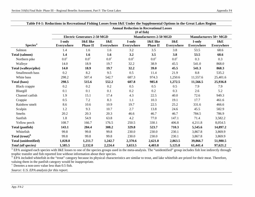
Section 316(b) Final Rule: Phase III – Regional Benefits Assessment, Part F: The Great Lakes Appendix F4
App. F4-2
Table F4-1: Reductions in Recreational Fishing Losses from I&E Under the Supplemental Options in the Great Lakes Region Annual Reduction in Recreational Losses
(# of fish) Electric Generators 2-50 MGD Manufacturers 2-50 MGD Manufacturers 50+ MGD
SpeciesP
aP
I-only Everywhere
I&E like Phase II
I&E Everywhere
I-only Everywhere
I&E like Phase II
I&E Everywhere
I-only Everywhere
I&E Everywhere
Salmon 1.4 1.6 1.6 3.2 3.5 3.8 53.5 68.6 Total (salmon) 1.4 1.6 1.6 3.2 3.5 3.8 53.5 68.6
Northern pike 0.0P
cP 0.0P
cP 0.0P
cP 0.0P
cP 0.0P
cP 0.0P
cP 0.3 0.3
Walleye 14.0 18.9 19.7 32.2 38.9 45.5 541.0 868.0 Total (walleye/pike) 14.0 18.9 19.7 32.2 39.0 45.5 541.3 868.3
Smallmouth bass 0.2 8.2 9.5 0.5 11.4 21.9 8.8 535.2 White bass 298.2 507.4 542.7 687.3 974.3 1,250.6 11,557.6 25,401.6
Total (bass) 298.5 515.6 552.2 687.8 985.8 1,272.5 11,566.5 25,936.8 Black crappie 0.2 0.2 0.2 0.5 0.5 0.5 7.9 7.9 Bluegill 0.1 0.1 0.1 0.2 0.2 0.3 2.6 5.2 Channel catfish 1.9 15.1 17.4 4.3 22.5 40.0 72.6 949.3 Crappie 0.5 7.2 8.3 1.1 10.3 19.1 17.7 461.6 Rainbow smelt 8.6 10.6 10.9 19.7 22.5 25.2 331.6 466.6 Sculpin 1.2 9.3 10.7 2.7 13.8 24.6 45.5 582.9 Smelts 20.2 20.3 20.3 46.6 46.7 46.7 784.5 786.9 Sunfish 1.8 54.9 63.8 4.2 77.0 147.1 71.4 3,582.2 Yellow perch 108.7 166.7 176.5 250.5 330.1 406.8 4,211.8 8,054.5
Total (panfish) 143.1 284.4 308.2 329.8 523.7 710.3 5,545.6 14,897.2 Whitefish 99.8 99.8 99.8 230.0 230.0 230.1 3,867.8 3,869.9
Total (trout)P
bP 99.8 99.8 99.8 230.0 230.0 230.1 3,867.8 3,869.9
Total (unidentified) 1,028.8 1,211.7 1,242.7 2,370.6 2,621.8 2,863.5 39,866.7 51,980.5 Total (all species) 1,585.5 2,132.0 2,224.4 3,653.5 4,403.8 5,125.8 61,441.4 97,621.2 P
aP EPA assigned each species with I&E losses to one of the species groups used in the meta-analysis. The “unidentified” group includes fish lost indirectly through
trophic transfer and fish reported lost without information about their species. P
bP EPA included whitefish in the “trout” category because its physical characteristics are similar to trout, and lake whitefish are prized for their meat. Therefore,
valuing them in the panfish category would be inappropriate. P
cP Denotes a non-zero value less than 0.5 fish.
Source: U.S. EPA analysis for this report.
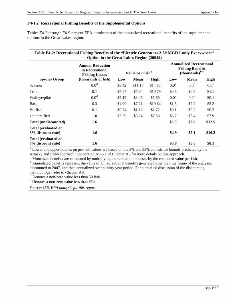
Section 316(b) Final Rule: Phase III – Regional Benefits Assessment, Part F: The Great Lakes Appendix F4
App. F4-3
F4-1.2 Recreational Fishing Benefits of the Supplemental Options Tables F4-2 through F4-9 present EPA’s estimates of the annualized recreational benefits of the supplemental options in the Great Lakes region.
Table F4-2: Recreational Fishing Benefits of the “Electric Generators 2-50 MGD I-only Everywhere” Option in the Great Lakes Region (2004$)
Value per FishP
aP
Annualized Recreational Fishing Benefits (thousands)P
b,cP
Species Group
Annual Reduction in Recreational Fishing Losses
(thousands of fish) Low Mean High Low Mean High Salmon 0.0P
dP $8.42 $11.17 $14.83 0.0P
eP 0.0P
eP 0.0P
eP
Trout 0.1 $5.87 $7.94 $10.79 $0.6 $0.8 $1.1 Walleye/pike 0.0P
dP $2.12 $3.46 $5.69 0.0P
eP 0.0P
eP $0.1
Bass 0.3 $4.90 $7.21 $10.64 $1.5 $2.2 $3.2 Panfish 0.1 $0.74 $1.12 $1.72 $0.1 $0.2 $0.2 Unidentified 1.0 $3.59 $5.24 $7.68 $3.7 $5.4 $7.9 Total (undiscounted) 1.6 $5.9 $8.6 $12.5 Total (evaluated at 3% discount rate) 1.6 $4.9 $7.1 $10.3 Total (evaluated at 7% discount rate) 1.6 $3.8 $5.6 $8.1 P
aP Lower and upper bounds on per-fish values are based on the 5% and 95% confidence bounds predicted by the
Krinsky and Robb approach. See section A5-5.1 of Chapter A5 for more details on this approach. P
bP Monetized benefits are calculated by multiplying the reduction in losses by the estimated value per fish.
P
cP Annualized benefits represent the value of all recreational benefits generated over the time frame of the analysis,
discounted to 2007, and then annualized over a thirty year period. For a detailed discussion of the discounting methodology, refer to Chapter A8. P
dP Denotes a non-zero value less than 50 fish.
P
eP Denotes a non-zero value less than $50.
Source: U.S. EPA analysis for this report.

Section 316(b) Final Rule: Phase III – Regional Benefits Assessment, Part F: The Great Lakes Appendix F4
App. F4-4
Table F4-3: Recreational Fishing Benefits of the “Electric Generators 2-50 MGD I&E like Phase II” Option in the Great Lakes Region (2004$)
Value per FishP
aP
Annualized Recreational Fishing Benefits (thousands)P
b,cP
Species Group
Annual Reduction in Recreational Fishing Losses
(thousands of fish) Low Mean High Low Mean High Salmon 0.0P
dP $8.42 $11.17 $14.83 0.0P
eP 0.0P
eP 0.0P
eP
Trout 0.1 $5.87 $7.94 $10.79 $0.6 $0.8 $1.1 Walleye/pike 0.0P
dP $2.12 $3.46 $5.69 0.0P
eP $0.1 $0.1
Bass 0.5 $4.90 $7.21 $10.64 $2.5 $3.7 $5.5 Panfish 0.3 $0.74 $1.12 $1.72 $0.2 $0.3 $0.5 Unidentified 1.2 $3.59 $5.24 $7.68 $4.4 $6.3 $9.3 Total (undiscounted) 2.1 $7.7 $11.3 $16.5 Total (evaluated at 3% discount rate) 2.1 $6.4 $9.3 $13.6 Total (evaluated at 7% discount rate) 2.1 $5.0 $7.3 $10.7 P
aP Lower and upper bounds on per-fish values are based on the 5% and 95% confidence bounds predicted by the
Krinsky and Robb approach. See section A5-5.1 of Chapter A5 for more details on this approach. P
bP Monetized benefits are calculated by multiplying the reduction in losses by the estimated value per fish.
P
cP Annualized benefits represent the value of all recreational benefits generated over the time frame of the analysis,
discounted to 2007, and then annualized over a thirty year period. For a detailed discussion of the discounting methodology, refer to Chapter A8. P
dP Denotes a non-zero value less than 50 fish.
P
eP Denotes a non-zero value less than $50.
Source: U.S. EPA analysis for this report.
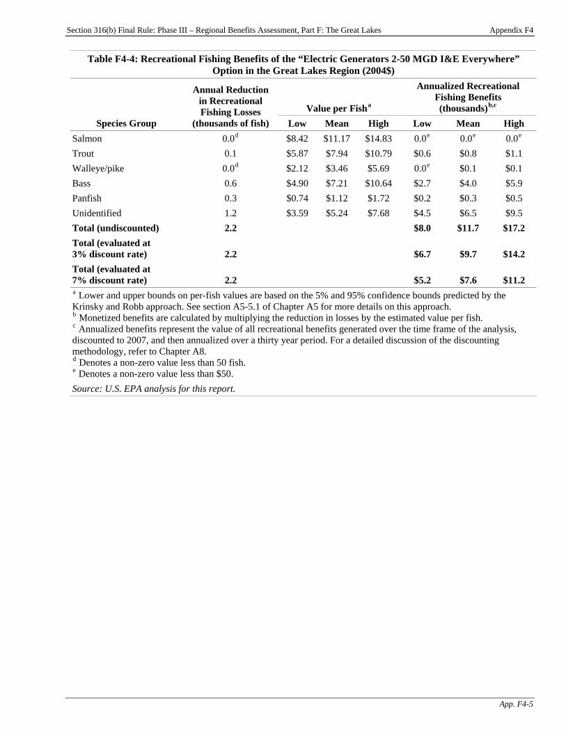
Section 316(b) Final Rule: Phase III – Regional Benefits Assessment, Part F: The Great Lakes Appendix F4
App. F4-5
Table F4-4: Recreational Fishing Benefits of the “Electric Generators 2-50 MGD I&E Everywhere” Option in the Great Lakes Region (2004$)
Value per FishP
aP
Annualized Recreational Fishing Benefits (thousands)P
b,cP
Species Group
Annual Reduction in Recreational Fishing Losses
(thousands of fish) Low Mean High Low Mean High Salmon 0.0P
dP $8.42 $11.17 $14.83 0.0P
eP 0.0P
eP 0.0P
eP
Trout 0.1 $5.87 $7.94 $10.79 $0.6 $0.8 $1.1 Walleye/pike 0.0P
dP $2.12 $3.46 $5.69 0.0P
eP $0.1 $0.1
Bass 0.6 $4.90 $7.21 $10.64 $2.7 $4.0 $5.9 Panfish 0.3 $0.74 $1.12 $1.72 $0.2 $0.3 $0.5 Unidentified 1.2 $3.59 $5.24 $7.68 $4.5 $6.5 $9.5 Total (undiscounted) 2.2 $8.0 $11.7 $17.2 Total (evaluated at 3% discount rate) 2.2 $6.7 $9.7 $14.2 Total (evaluated at 7% discount rate) 2.2 $5.2 $7.6 $11.2 P
aP Lower and upper bounds on per-fish values are based on the 5% and 95% confidence bounds predicted by the
Krinsky and Robb approach. See section A5-5.1 of Chapter A5 for more details on this approach. P
bP Monetized benefits are calculated by multiplying the reduction in losses by the estimated value per fish.
P
cP Annualized benefits represent the value of all recreational benefits generated over the time frame of the analysis,
discounted to 2007, and then annualized over a thirty year period. For a detailed discussion of the discounting methodology, refer to Chapter A8. P
dP Denotes a non-zero value less than 50 fish.
P
eP Denotes a non-zero value less than $50.
Source: U.S. EPA analysis for this report.
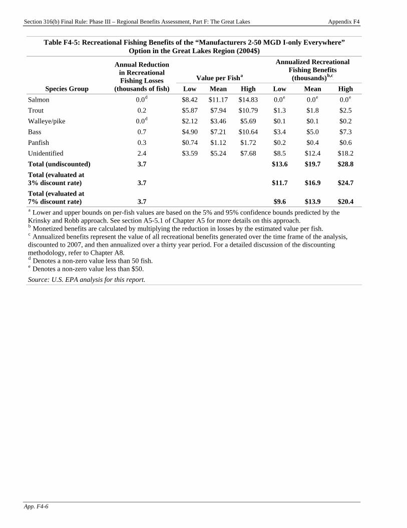
Section 316(b) Final Rule: Phase III – Regional Benefits Assessment, Part F: The Great Lakes Appendix F4
App. F4-6
Table F4-5: Recreational Fishing Benefits of the “Manufacturers 2-50 MGD I-only Everywhere” Option in the Great Lakes Region (2004$)
Value per FishP
aP
Annualized Recreational Fishing Benefits (thousands)P
b,cP
Species Group
Annual Reduction in Recreational Fishing Losses
(thousands of fish) Low Mean High Low Mean High Salmon 0.0P
dP $8.42 $11.17 $14.83 0.0P
eP 0.0P
eP 0.0P
eP
Trout 0.2 $5.87 $7.94 $10.79 $1.3 $1.8 $2.5 Walleye/pike 0.0P
dP $2.12 $3.46 $5.69 $0.1 $0.1 $0.2
Bass 0.7 $4.90 $7.21 $10.64 $3.4 $5.0 $7.3 Panfish 0.3 $0.74 $1.12 $1.72 $0.2 $0.4 $0.6 Unidentified 2.4 $3.59 $5.24 $7.68 $8.5 $12.4 $18.2 Total (undiscounted) 3.7 $13.6 $19.7 $28.8 Total (evaluated at 3% discount rate) 3.7 $11.7 $16.9 $24.7 Total (evaluated at 7% discount rate) 3.7 $9.6 $13.9 $20.4 P
aP Lower and upper bounds on per-fish values are based on the 5% and 95% confidence bounds predicted by the
Krinsky and Robb approach. See section A5-5.1 of Chapter A5 for more details on this approach. P
bP Monetized benefits are calculated by multiplying the reduction in losses by the estimated value per fish.
P
cP Annualized benefits represent the value of all recreational benefits generated over the time frame of the analysis,
discounted to 2007, and then annualized over a thirty year period. For a detailed discussion of the discounting methodology, refer to Chapter A8. P
dP Denotes a non-zero value less than 50 fish.
P
eP Denotes a non-zero value less than $50.
Source: U.S. EPA analysis for this report.
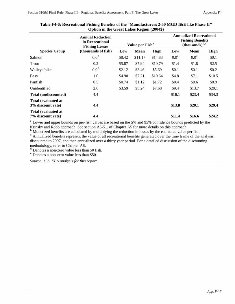
Section 316(b) Final Rule: Phase III – Regional Benefits Assessment, Part F: The Great Lakes Appendix F4
App. F4-7
Table F4-6: Recreational Fishing Benefits of the “Manufacturers 2-50 MGD I&E like Phase II” Option in the Great Lakes Region (2004$)
Value per FishP
aP
Annualized Recreational Fishing Benefits (thousands)P
b,cP
Species Group
Annual Reduction in Recreational Fishing Losses
(thousands of fish) Low Mean High Low Mean High Salmon 0.0P
dP $8.42 $11.17 $14.83 0.0P
eP 0.0P
eP $0.1
Trout 0.2 $5.87 $7.94 $10.79 $1.4 $1.8 $2.5 Walleye/pike 0.0P
dP $2.12 $3.46 $5.69 $0.1 $0.1 $0.2
Bass 1.0 $4.90 $7.21 $10.64 $4.8 $7.1 $10.5 Panfish 0.5 $0.74 $1.12 $1.72 $0.4 $0.6 $0.9 Unidentified 2.6 $3.59 $5.24 $7.68 $9.4 $13.7 $20.1 Total (undiscounted) 4.4 $16.1 $23.4 $34.3 Total (evaluated at 3% discount rate) 4.4 $13.8 $20.1 $29.4 Total (evaluated at 7% discount rate) 4.4 $11.4 $16.6 $24.2 P
aP Lower and upper bounds on per-fish values are based on the 5% and 95% confidence bounds predicted by the
Krinsky and Robb approach. See section A5-5.1 of Chapter A5 for more details on this approach. P
bP Monetized benefits are calculated by multiplying the reduction in losses by the estimated value per fish.
P
cP Annualized benefits represent the value of all recreational benefits generated over the time frame of the analysis,
discounted to 2007, and then annualized over a thirty year period. For a detailed discussion of the discounting methodology, refer to Chapter A8. P
dP Denotes a non-zero value less than 50 fish.
P
eP Denotes a non-zero value less than $50.
Source: U.S. EPA analysis for this report.

Section 316(b) Final Rule: Phase III – Regional Benefits Assessment, Part F: The Great Lakes Appendix F4
App. F4-8
Table F4-7: Recreational Fishing Benefits of the “Manufacturers 2-50 MGD I&E Everywhere” Option in the Great Lakes Region (2004$)
Value per FishP
aP
Annualized Recreational Fishing Benefits (thousands)P
b,cP
Species Group
Annual Reduction in Recreational Fishing Losses
(thousands of fish) Low Mean High Low Mean High Salmon 0.0P
dP $8.42 $11.17 $14.83 0.0P
eP 0.0P
eP $0.1
Trout 0.2 $5.87 $7.94 $10.79 $1.4 $1.8 $2.5 Walleye/pike 0.0P
dP $2.12 $3.46 $5.69 $0.1 $0.2 $0.3
Bass 1.3 $4.90 $7.21 $10.64 $6.2 $9.2 $13.5 Panfish 0.7 $0.74 $1.12 $1.72 $0.5 $0.8 $1.2 Unidentified 2.9 $3.59 $5.24 $7.68 $10.3 $15.0 $22.0 Total (undiscounted) 5.1 $18.5 $27.0 $39.5 Total (evaluated at 3% discount rate) 5.1 $15.9 $23.2 $33.9 Total (evaluated at 7% discount rate) 5.1 $13.1 $19.1 $28.0 P
aP Lower and upper bounds on per-fish values are based on the 5% and 95% confidence bounds predicted by the
Krinsky and Robb approach. See section A5-5.1 of Chapter A5 for more details on this approach. P
bP Monetized benefits are calculated by multiplying the reduction in losses by the estimated value per fish.
P
cP Annualized benefits represent the value of all recreational benefits generated over the time frame of the analysis,
discounted to 2007, and then annualized over a thirty year period. For a detailed discussion of the discounting methodology, refer to Chapter A8. P
dP Denotes a non-zero value less than 50 fish.
P
eP Denotes a non-zero value less than $50.
Source: U.S. EPA analysis for this report.
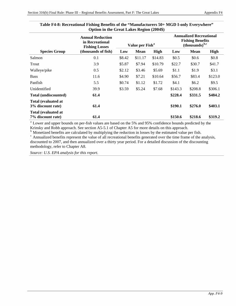
Section 316(b) Final Rule: Phase III – Regional Benefits Assessment, Part F: The Great Lakes Appendix F4
App. F4-9
Table F4-8: Recreational Fishing Benefits of the “Manufacturers 50+ MGD I-only Everywhere” Option in the Great Lakes Region (2004$)
Value per FishP
aP
Annualized Recreational Fishing Benefits (thousands)P
b,cP
Species Group
Annual Reduction in Recreational Fishing Losses
(thousands of fish) Low Mean High Low Mean High Salmon 0.1 $8.42 $11.17 $14.83 $0.5 $0.6 $0.8 Trout 3.9 $5.87 $7.94 $10.79 $22.7 $30.7 $41.7 Walleye/pike 0.5 $2.12 $3.46 $5.69 $1.1 $1.9 $3.1 Bass 11.6 $4.90 $7.21 $10.64 $56.7 $83.4 $123.0 Panfish 5.5 $0.74 $1.12 $1.72 $4.1 $6.2 $9.5 Unidentified 39.9 $3.59 $5.24 $7.68 $143.3 $208.8 $306.1 Total (undiscounted) 61.4 $228.4 $331.5 $484.2 Total (evaluated at 3% discount rate) 61.4 $190.1 $276.0 $403.1 Total (evaluated at 7% discount rate) 61.4 $150.6 $218.6 $319.2 P
aP Lower and upper bounds on per-fish values are based on the 5% and 95% confidence bounds predicted by the
Krinsky and Robb approach. See section A5-5.1 of Chapter A5 for more details on this approach. P
bP Monetized benefits are calculated by multiplying the reduction in losses by the estimated value per fish.
P
cP Annualized benefits represent the value of all recreational benefits generated over the time frame of the analysis,
discounted to 2007, and then annualized over a thirty year period. For a detailed discussion of the discounting methodology, refer to Chapter A8. Source: U.S. EPA analysis for this report.
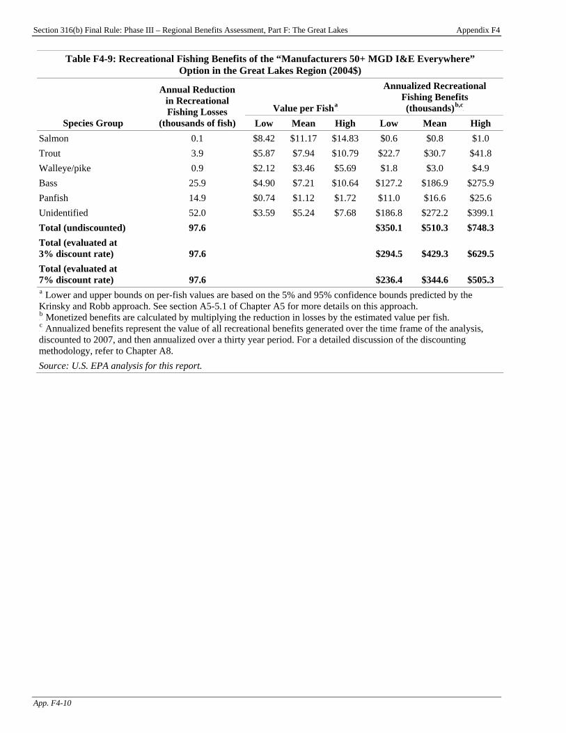
Section 316(b) Final Rule: Phase III – Regional Benefits Assessment, Part F: The Great Lakes Appendix F4
App. F4-10
Table F4-9: Recreational Fishing Benefits of the “Manufacturers 50+ MGD I&E Everywhere” Option in the Great Lakes Region (2004$)
Value per FishP
aP
Annualized Recreational Fishing Benefits (thousands)P
b,cP
Species Group
Annual Reduction in Recreational Fishing Losses
(thousands of fish) Low Mean High Low Mean High Salmon 0.1 $8.42 $11.17 $14.83 $0.6 $0.8 $1.0 Trout 3.9 $5.87 $7.94 $10.79 $22.7 $30.7 $41.8 Walleye/pike 0.9 $2.12 $3.46 $5.69 $1.8 $3.0 $4.9 Bass 25.9 $4.90 $7.21 $10.64 $127.2 $186.9 $275.9 Panfish 14.9 $0.74 $1.12 $1.72 $11.0 $16.6 $25.6 Unidentified 52.0 $3.59 $5.24 $7.68 $186.8 $272.2 $399.1 Total (undiscounted) 97.6 $350.1 $510.3 $748.3 Total (evaluated at 3% discount rate) 97.6 $294.5 $429.3 $629.5 Total (evaluated at 7% discount rate) 97.6 $236.4 $344.6 $505.3 P
aP Lower and upper bounds on per-fish values are based on the 5% and 95% confidence bounds predicted by the
Krinsky and Robb approach. See section A5-5.1 of Chapter A5 for more details on this approach. P
bP Monetized benefits are calculated by multiplying the reduction in losses by the estimated value per fish.
P
cP Annualized benefits represent the value of all recreational benefits generated over the time frame of the analysis,
discounted to 2007, and then annualized over a thirty year period. For a detailed discussion of the discounting methodology, refer to Chapter A8. Source: U.S. EPA analysis for this report.

Section 316(b) Final Rule: Phase III – Regional Benefits Assessment, Part F: The Great Lakes Appendix F4
App. F4-11
F4-2 Comparison of Recreational Fishing Benefits by Option Table F4-10 compares the recreational fishing benefits of the eight supplemental options.
Table F4-10: Annual Recreational Benefits of the Supplemental Options in the Great Lakes Region Undiscounted Recreational Fishing Benefits
(thousands; 2004$)P
aP
Policy Option
Annual Reduction in Recreational Fishing
Losses from I&E (thousands of fish) Low Mean High
Electric Generators 2-50 MGD I-only Everywhere 1.6 $5.9 $8.6 $12.5 I&E like Phase II 2.1 $7.7 $11.3 $16.5 I&E Everywhere 2.2 $8.0 $11.7 $17.2
Manufacturers 2-50 MGD I-only Everywhere 3.7 $13.6 $19.7 $28.8 I&E like Phase II 4.4 $16.1 $23.4 $34.3 I&E Everywhere 5.1 $18.5 $27.0 $39.5
Manufacturers 50+ MGD I-only Everywhere 61.4 $228.4 $331.5 $484.2 I&E Everywhere 97.6 $350.1 $510.3 $748.3
P
aP These benefit estimates were calculated using the meta-analysis approach discussed in Chapter A5 and Chapter B4.
Source: U.S. EPA analysis for this report.
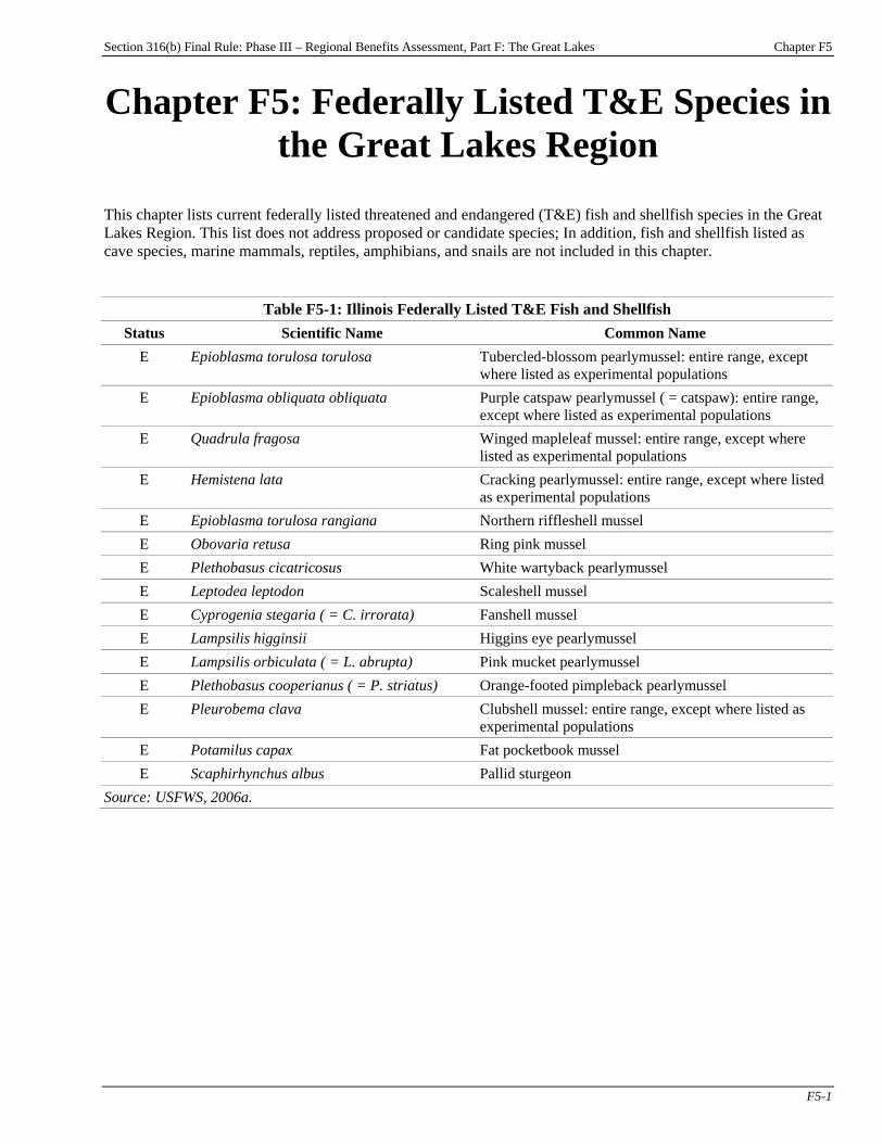
Section 316(b) Final Rule: Phase III – Regional Benefits Assessment, Part F: The Great Lakes Chapter F5
F5-1
Chapter F5: Federally Listed T&E Species in the Great Lakes Region
This chapter lists current federally listed threatened and endangered (T&E) fish and shellfish species in the Great Lakes Region. This list does not address proposed or candidate species; In addition, fish and shellfish listed as cave species, marine mammals, reptiles, amphibians, and snails are not included in this chapter.
Table F5-1: Illinois Federally Listed T&E Fish and Shellfish Status Scientific Name Common Name
E Epioblasma torulosa torulosa Tubercled-blossom pearlymussel: entire range, except where listed as experimental populations
E Epioblasma obliquata obliquata Purple catspaw pearlymussel ( = catspaw): entire range, except where listed as experimental populations
E Quadrula fragosa Winged mapleleaf mussel: entire range, except where listed as experimental populations
E Hemistena lata Cracking pearlymussel: entire range, except where listed as experimental populations
E Epioblasma torulosa rangiana Northern riffleshell mussel E Obovaria retusa Ring pink mussel E Plethobasus cicatricosus White wartyback pearlymussel E Leptodea leptodon Scaleshell mussel E Cyprogenia stegaria ( = C. irrorata) Fanshell mussel E Lampsilis higginsii Higgins eye pearlymussel E Lampsilis orbiculata ( = L. abrupta) Pink mucket pearlymussel E Plethobasus cooperianus ( = P. striatus) Orange-footed pimpleback pearlymussel E Pleurobema clava Clubshell mussel: entire range, except where listed as
experimental populations E Potamilus capax Fat pocketbook mussel E Scaphirhynchus albus Pallid sturgeon
Source: USFWS, 2006a.
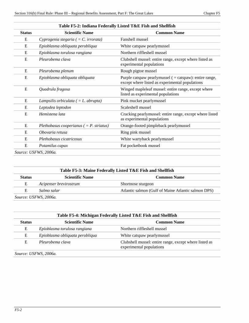
Section 316(b) Final Rule: Phase III – Regional Benefits Assessment, Part F: The Great Lakes Chapter F5
F5-2
Table F5-2: Indiana Federally Listed T&E Fish and Shellfish Status Scientific Name Common Name
E Cyprogenia stegaria ( = C. irrorata) Fanshell mussel E Epioblasma obliquata perobliqua White catspaw pearlymussel E Epioblasma torulosa rangiana Northern riffleshell mussel E Pleurobema clava Clubshell mussel: entire range, except where listed as
experimental populations E Pleurobema plenum Rough pigtoe mussel E Epioblasma obliquata obliquata Purple catspaw pearlymussel ( = catspaw): entire range,
except where listed as experimental populations E Quadrula fragosa Winged mapleleaf mussel: entire range, except where
listed as experimental populations E Lampsilis orbiculata ( = L. abrupta) Pink mucket pearlymussel E Leptodea leptodon Scaleshell mussel E Hemistena lata Cracking pearlymussel: entire range, except where listed
as experimental populations E Plethobasus cooperianus ( = P. striatus) Orange-footed pimpleback pearlymussel E Obovaria retusa Ring pink mussel E Plethobasus cicatricosus White wartyback pearlymussel E Potamilus capax Fat pocketbook mussel
Source: USFWS, 2006a.
Table F5-3: Maine Federally Listed T&E Fish and Shellfish Status Scientific Name Common Name
E Acipenser brevirostrum Shortnose sturgeon E Salmo salar Atlantic salmon (Gulf of Maine Atlantic salmon DPS)
Source: USFWS, 2006a.
Table F5-4: Michigan Federally Listed T&E Fish and Shellfish Status Scientific Name Common Name
E Epioblasma torulosa rangiana Northern riffleshell mussel E Epioblasma obliquata perobliqua White catspaw pearlymussel E Pleurobema clava Clubshell mussel: entire range, except where listed as
experimental populations Source: USFWS, 2006a.
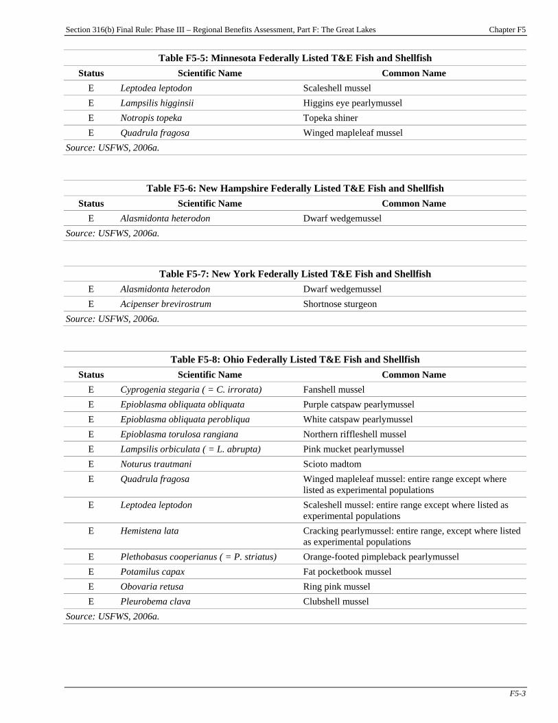
Section 316(b) Final Rule: Phase III – Regional Benefits Assessment, Part F: The Great Lakes Chapter F5
F5-3
Table F5-5: Minnesota Federally Listed T&E Fish and Shellfish Status Scientific Name Common Name
E Leptodea leptodon Scaleshell mussel E Lampsilis higginsii Higgins eye pearlymussel E Notropis topeka Topeka shiner E Quadrula fragosa Winged mapleleaf mussel
Source: USFWS, 2006a.
Table F5-6: New Hampshire Federally Listed T&E Fish and Shellfish Status Scientific Name Common Name
E Alasmidonta heterodon Dwarf wedgemussel Source: USFWS, 2006a.
Table F5-7: New York Federally Listed T&E Fish and Shellfish E Alasmidonta heterodon Dwarf wedgemussel E Acipenser brevirostrum Shortnose sturgeon
Source: USFWS, 2006a.
Table F5-8: Ohio Federally Listed T&E Fish and Shellfish Status Scientific Name Common Name
E Cyprogenia stegaria ( = C. irrorata) Fanshell mussel E Epioblasma obliquata obliquata Purple catspaw pearlymussel E Epioblasma obliquata perobliqua White catspaw pearlymussel E Epioblasma torulosa rangiana Northern riffleshell mussel E Lampsilis orbiculata ( = L. abrupta) Pink mucket pearlymussel E Noturus trautmani Scioto madtom E Quadrula fragosa Winged mapleleaf mussel: entire range except where
listed as experimental populations E Leptodea leptodon Scaleshell mussel: entire range except where listed as
experimental populations E Hemistena lata Cracking pearlymussel: entire range, except where listed
as experimental populations E Plethobasus cooperianus ( = P. striatus) Orange-footed pimpleback pearlymussel E Potamilus capax Fat pocketbook mussel E Obovaria retusa Ring pink mussel E Pleurobema clava Clubshell mussel
Source: USFWS, 2006a.
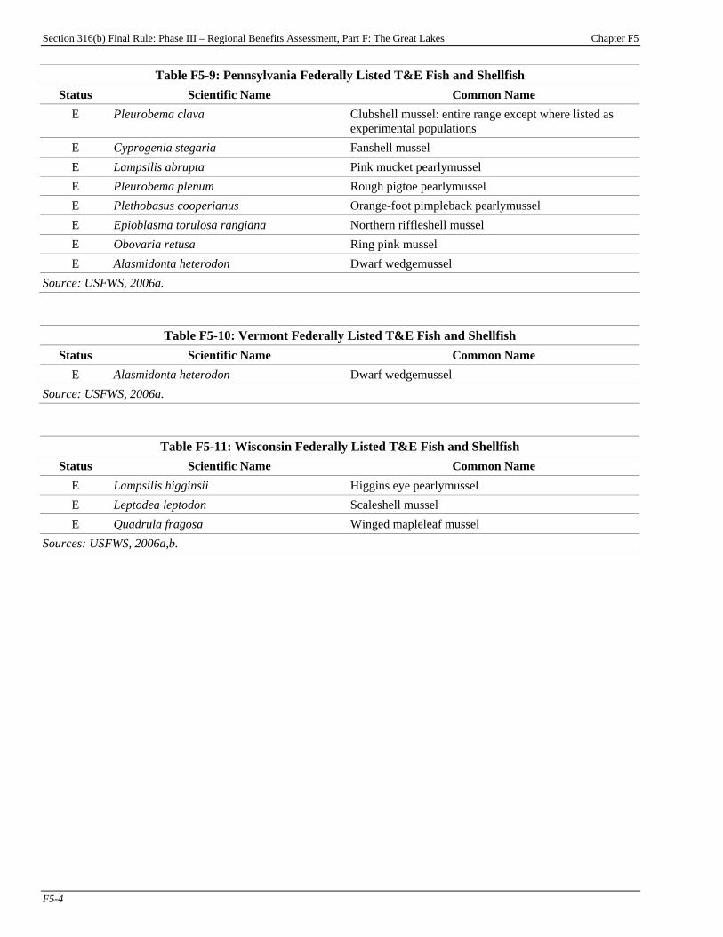
Section 316(b) Final Rule: Phase III – Regional Benefits Assessment, Part F: The Great Lakes Chapter F5
F5-4
Table F5-9: Pennsylvania Federally Listed T&E Fish and Shellfish Status Scientific Name Common Name
E Pleurobema clava Clubshell mussel: entire range except where listed as experimental populations
E Cyprogenia stegaria Fanshell mussel E Lampsilis abrupta Pink mucket pearlymussel E Pleurobema plenum Rough pigtoe pearlymussel E Plethobasus cooperianus Orange-foot pimpleback pearlymussel E Epioblasma torulosa rangiana Northern riffleshell mussel E Obovaria retusa Ring pink mussel E Alasmidonta heterodon Dwarf wedgemussel
Source: USFWS, 2006a.
Table F5-10: Vermont Federally Listed T&E Fish and Shellfish Status Scientific Name Common Name
E Alasmidonta heterodon Dwarf wedgemussel Source: USFWS, 2006a.
Table F5-11: Wisconsin Federally Listed T&E Fish and Shellfish Status Scientific Name Common Name
E Lampsilis higginsii Higgins eye pearlymussel E Leptodea leptodon Scaleshell mussel E Quadrula fragosa Winged mapleleaf mussel
Sources: USFWS, 2006a,b.

Section 316(b) Final Rule: Phase III – Regional Benefits Assessment
Part G: The Inland Region

Section 316(b) Final Rule: Phase III – Regional Benefits Assessment, Part G: The Inland Region Chapter G1
G1-1
Chapter G1: Background Introduction This chapter presents an overview of the potential Phase III existing facilities in the Inland study region and summarizes their key cooling water and compliance characteristics. For further discussion of the technical and compliance characteristics of potential Phase III existing facilities, refer to the Economic Analysis for the Final Section 316(b) Rule for Phase III Facilities and the Technical Development Document for the Final Section 316(b) Rule for Phase III Facilities (U.S. EPA, 2006a,c).
Chapter Contents G1-1 Facility Characteristics..................................G1-1
G1-1 Facility Characteristics The Inland Regional Study includes 274 sample facilities that are potentially subject to the national standards for Phase III existing facilities. Figure G1-1 presents a map of these facilities. One hundred and seventy-two facilities are manufacturing facilities and 102 are electric generators. Industry-wide, these 274 sample facilities represent 541 facilities.PF
1FP
P
1P EPA applied sample weights to the survey respondents to account for non-sampled facilities and facilities that did
not respond to the survey. For more information on EPA’s 2000 Section 316(b) Industry Survey, please refer to the Information Collection Request (U.S. EPA, 2000b).
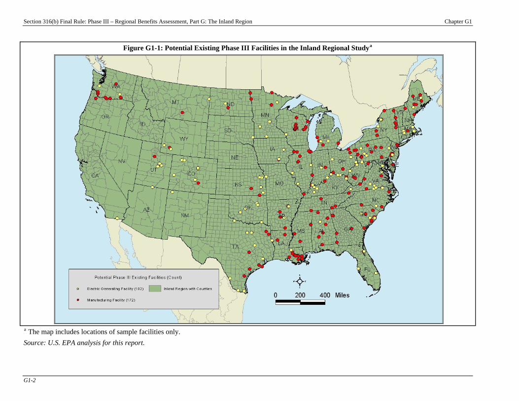
Section 316(b) Final Rule: Phase III – Regional Benefits Assessment, Part G: The Inland Region Chapter G1
G1-2
Figure G1-1: Potential Existing Phase III Facilities in the Inland Regional StudyP
aP
P
aP The map includes locations of sample facilities only.
Source: U.S. EPA analysis for this report.
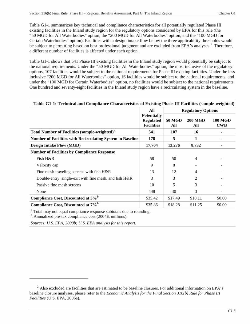
Section 316(b) Final Rule: Phase III – Regional Benefits Assessment, Part G: The Inland Region Chapter G1
G1-3
Table G1-1 summarizes key technical and compliance characteristics for all potentially regulated Phase III existing facilities in the Inland study region for the regulatory options considered by EPA for this rule (the “50 MGD for All Waterbodies” option, the “200 MGD for All Waterbodies” option, and the “100 MGD for Certain Waterbodies” option). Facilities with a design intake flow below the three applicability thresholds would be subject to permitting based on best professional judgment and are excluded from EPA’s analyses.PF
2FP Therefore,
a different number of facilities is affected under each option. Table G1-1 shows that 541 Phase III existing facilities in the Inland study region would potentially be subject to the national requirements. Under the “50 MGD for All Waterbodies” option, the most inclusive of the regulatory options, 107 facilities would be subject to the national requirements for Phase III existing facilities. Under the less inclusive “200 MGD for All Waterbodies” option, 16 facilities would be subject to the national requirements, and under the “100 MGD for Certain Waterbodies” option, no facilities would be subject to the national requirements. One hundred and seventy-eight facilities in the Inland study region have a recirculating system in the baseline.
Table G1-1: Technical and Compliance Characteristics of Existing Phase III Facilities (sample-weighted)Regulatory Options All
Potentially Regulated Facilities
50 MGD All
200 MGD All
100 MGD CWB
Total Number of Facilities (sample-weighted)P
aP 541 107 16 -
Number of Facilities with Recirculating System in Baseline 178 5 1 - Design Intake Flow (MGD) 17,704 13,276 8,732 - Number of Facilities by Compliance Response
Fish H&R 58 50 4 - Velocity cap 9 8 - - Fine mesh traveling screens with fish H&R 13 12 4 - Double-entry, single-exit with fine mesh, and fish H&R 3 3 2 - Passive fine mesh screens 10 5 3 - None 448 30 3 -
Compliance Cost, Discounted at 3%P
bP $35.42 $17.49 $10.11 $0.00
Compliance Cost, Discounted at 7%P
bP $35.86 $18.28 $11.25 $0.00
P
aP Total may not equal compliance response subtotals due to rounding.
P
bP Annualized pre-tax compliance cost (2004$, millions).
Sources: U.S. EPA, 2000b; U.S. EPA analysis for this report.
P
2P Also excluded are facilities that are estimated to be baseline closures. For additional information on EPA’s
baseline closure analyses, please refer to the Economic Analysis for the Final Section 316(b) Rule for Phase III Facilities (U.S. EPA, 2006a).
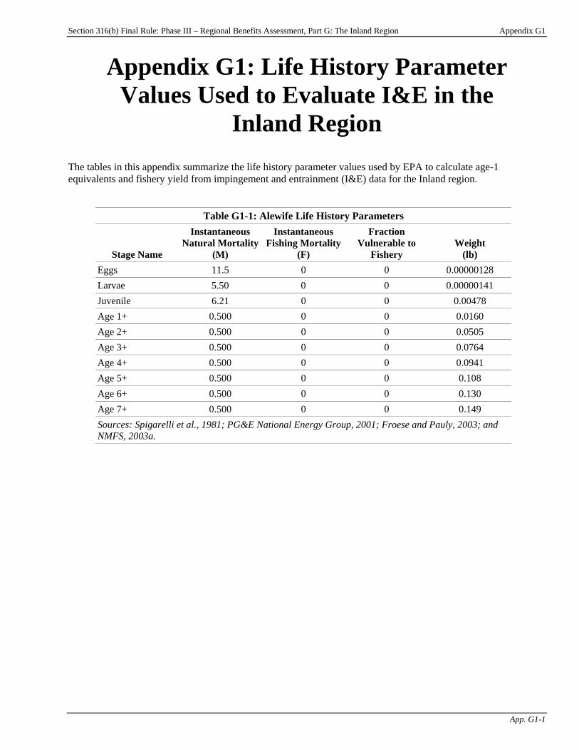
Section 316(b) Final Rule: Phase III – Regional Benefits Assessment, Part G: The Inland Region Appendix G1
App. G1-1
Appendix G1: Life History Parameter Values Used to Evaluate I&E in the
Inland Region The tables in this appendix summarize the life history parameter values used by EPA to calculate age-1 equivalents and fishery yield from impingement and entrainment (I&E) data for the Inland region.
Table G1-1: Alewife Life History Parameters
Stage Name
Instantaneous Natural Mortality
(M)
Instantaneous Fishing Mortality
(F)
Fraction Vulnerable to
Fishery Weight
(lb) Eggs 11.5 0 0 0.00000128 Larvae 5.50 0 0 0.00000141 Juvenile 6.21 0 0 0.00478 Age 1+ 0.500 0 0 0.0160 Age 2+ 0.500 0 0 0.0505 Age 3+ 0.500 0 0 0.0764 Age 4+ 0.500 0 0 0.0941 Age 5+ 0.500 0 0 0.108 Age 6+ 0.500 0 0 0.130 Age 7+ 0.500 0 0 0.149 Sources: Spigarelli et al., 1981; PG&E National Energy Group, 2001; Froese and Pauly, 2003; and NMFS, 2003a.
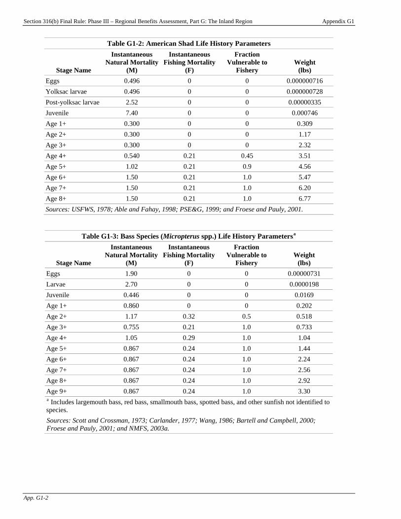
Section 316(b) Final Rule: Phase III – Regional Benefits Assessment, Part G: The Inland Region Appendix G1
App. G1-2
Table G1-2: American Shad Life History Parameters
Stage Name
Instantaneous Natural Mortality
(M)
Instantaneous Fishing Mortality
(F)
Fraction Vulnerable to
Fishery Weight
(lbs) Eggs 0.496 0 0 0.000000716 Yolksac larvae 0.496 0 0 0.000000728 Post-yolksac larvae 2.52 0 0 0.00000335 Juvenile 7.40 0 0 0.000746 Age 1+ 0.300 0 0 0.309 Age 2+ 0.300 0 0 1.17 Age 3+ 0.300 0 0 2.32 Age 4+ 0.540 0.21 0.45 3.51 Age 5+ 1.02 0.21 0.9 4.56 Age 6+ 1.50 0.21 1.0 5.47 Age 7+ 1.50 0.21 1.0 6.20 Age 8+ 1.50 0.21 1.0 6.77 Sources: USFWS, 1978; Able and Fahay, 1998; PSE&G, 1999; and Froese and Pauly, 2001.
Table G1-3: Bass Species (Micropterus spp.) Life History ParametersP
aP
Stage Name
Instantaneous Natural Mortality
(M)
Instantaneous Fishing Mortality
(F)
Fraction Vulnerable to
Fishery Weight
(lbs) Eggs 1.90 0 0 0.00000731 Larvae 2.70 0 0 0.0000198 Juvenile 0.446 0 0 0.0169 Age 1+ 0.860 0 0 0.202 Age 2+ 1.17 0.32 0.5 0.518 Age 3+ 0.755 0.21 1.0 0.733 Age 4+ 1.05 0.29 1.0 1.04 Age 5+ 0.867 0.24 1.0 1.44 Age 6+ 0.867 0.24 1.0 2.24 Age 7+ 0.867 0.24 1.0 2.56 Age 8+ 0.867 0.24 1.0 2.92 Age 9+ 0.867 0.24 1.0 3.30 P
aP Includes largemouth bass, red bass, smallmouth bass, spotted bass, and other sunfish not identified to
species. TSources: Scott and Crossman, 1973; Carlander, 1977; Wang, 1986; Bartell and Campbell, 2000; TFroese and Pauly, 2001; and NMFS, 2003a.
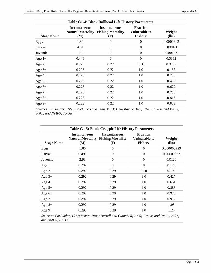
Section 316(b) Final Rule: Phase III – Regional Benefits Assessment, Part G: The Inland Region Appendix G1
App. G1-3
Table G1-4: Black Bullhead Life History Parameters
Stage Name
Instantaneous Natural Mortality
(M)
Instantaneous Fishing Mortality
(F)
Fraction Vulnerable to
Fishery Weight
(lbs) Eggs 1.90 0 0 0.0000312 Larvae 4.61 0 0 0.000186 Juvenile+ 1.39 0 0 0.00132 Age 1+ 0.446 0 0 0.0362 Age 2+ 0.223 0.22 0.50 0.0797 Age 3+ 0.223 0.22 1.0 0.137 Age 4+ 0.223 0.22 1.0 0.233 Age 5+ 0.223 0.22 1.0 0.402 Age 6+ 0.223 0.22 1.0 0.679 Age 7+ 0.223 0.22 1.0 0.753 Age 8+ 0.223 0.22 1.0 0.815 Age 9+ 0.223 0.22 1.0 0.823 TSources: Carlander, 1969; Scott and Crossman, 1973; Geo-Marine, Inc., 1978; Froese and Pauly, 2001; Tand NMFS, 2003a.
Table G1-5: Black Crappie Life History Parameters
Stage Name
Instantaneous Natural Mortality
(M)
Instantaneous Fishing Mortality
(F)
Fraction Vulnerable to
Fishery Weight
(lbs) Eggs 1.80 0 0 0.000000929 Larvae 0.498 0 0 0.00000857 Juvenile 2.93 0 0 0.0120 Age 1+ 0.292 0 0 0.128 Age 2+ 0.292 0.29 0.50 0.193 Age 3+ 0.292 0.29 1.0 0.427 Age 4+ 0.292 0.29 1.0 0.651 Age 5+ 0.292 0.29 1.0 0.888 Age 6+ 0.292 0.29 1.0 0.925 Age 7+ 0.292 0.29 1.0 0.972 Age 8+ 0.292 0.29 1.0 1.08 Age 9+ 0.292 0.29 1.0 1.26 Sources: Carlander, 1977; Wang, 1986; Bartell and Campbell, 2000; Froese and Pauly, 2001; and NMFS, 2003a.
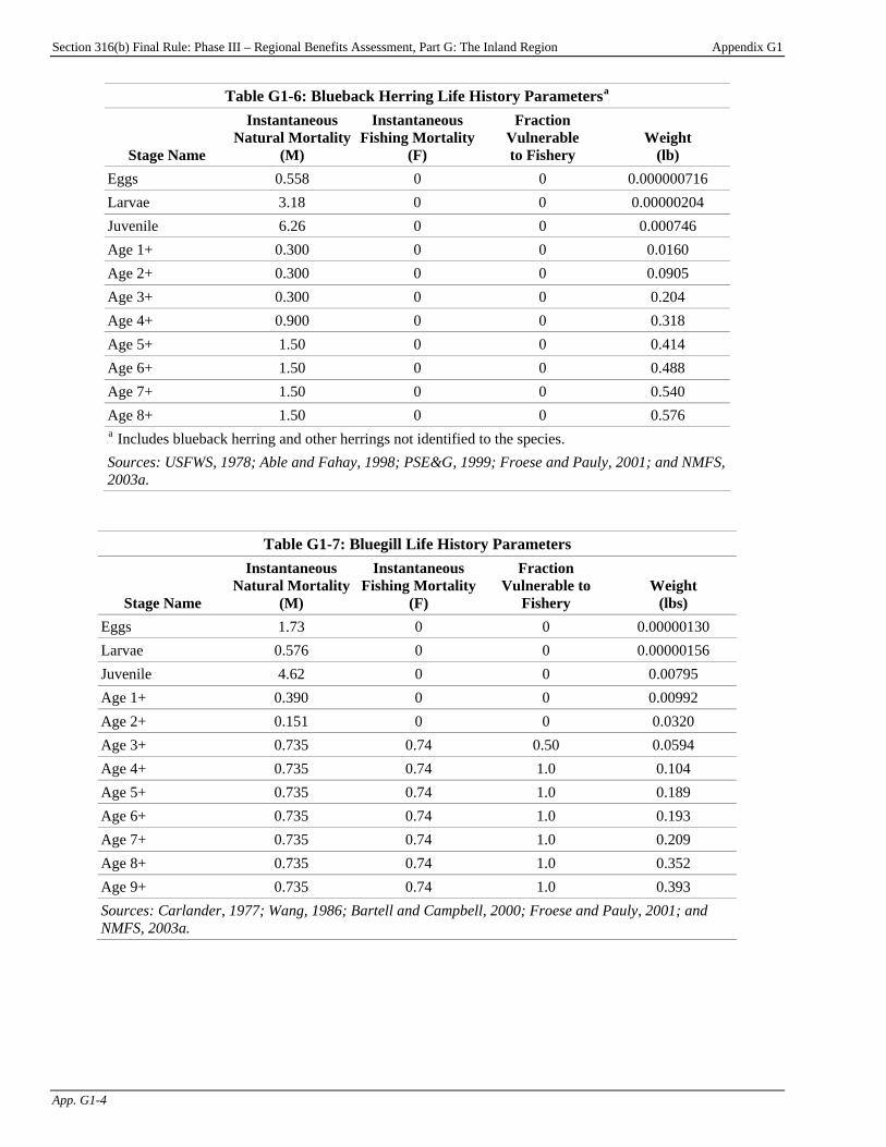
Section 316(b) Final Rule: Phase III – Regional Benefits Assessment, Part G: The Inland Region Appendix G1
App. G1-4
Table G1-6: Blueback Herring Life History ParametersP
aP
Stage Name
Instantaneous Natural Mortality
(M)
Instantaneous Fishing Mortality
(F)
Fraction Vulnerable to Fishery
Weight (lb)
Eggs 0.558 0 0 0.000000716 Larvae 3.18 0 0 0.00000204 Juvenile 6.26 0 0 0.000746 Age 1+ 0.300 0 0 0.0160 Age 2+ 0.300 0 0 0.0905 Age 3+ 0.300 0 0 0.204 Age 4+ 0.900 0 0 0.318 Age 5+ 1.50 0 0 0.414 Age 6+ 1.50 0 0 0.488 Age 7+ 1.50 0 0 0.540 Age 8+ 1.50 0 0 0.576 P
aP Includes blueback herring and other herrings not identified to the species.
Sources: USFWS, 1978; Able and Fahay, 1998; PSE&G, 1999; Froese and Pauly, 2001; and NMFS, 2003a.
Table G1-7: Bluegill Life History Parameters
Stage Name
Instantaneous Natural Mortality
(M)
Instantaneous Fishing Mortality
(F)
Fraction Vulnerable to
Fishery Weight
(lbs) Eggs 1.73 0 0 0.00000130 Larvae 0.576 0 0 0.00000156 Juvenile 4.62 0 0 0.00795 Age 1+ 0.390 0 0 0.00992 Age 2+ 0.151 0 0 0.0320 Age 3+ 0.735 0.74 0.50 0.0594 Age 4+ 0.735 0.74 1.0 0.104 Age 5+ 0.735 0.74 1.0 0.189 Age 6+ 0.735 0.74 1.0 0.193 Age 7+ 0.735 0.74 1.0 0.209 Age 8+ 0.735 0.74 1.0 0.352 Age 9+ 0.735 0.74 1.0 0.393 Sources: Carlander, 1977; Wang, 1986; Bartell and Campbell, 2000; Froese and Pauly, 2001; and NMFS, 2003a.
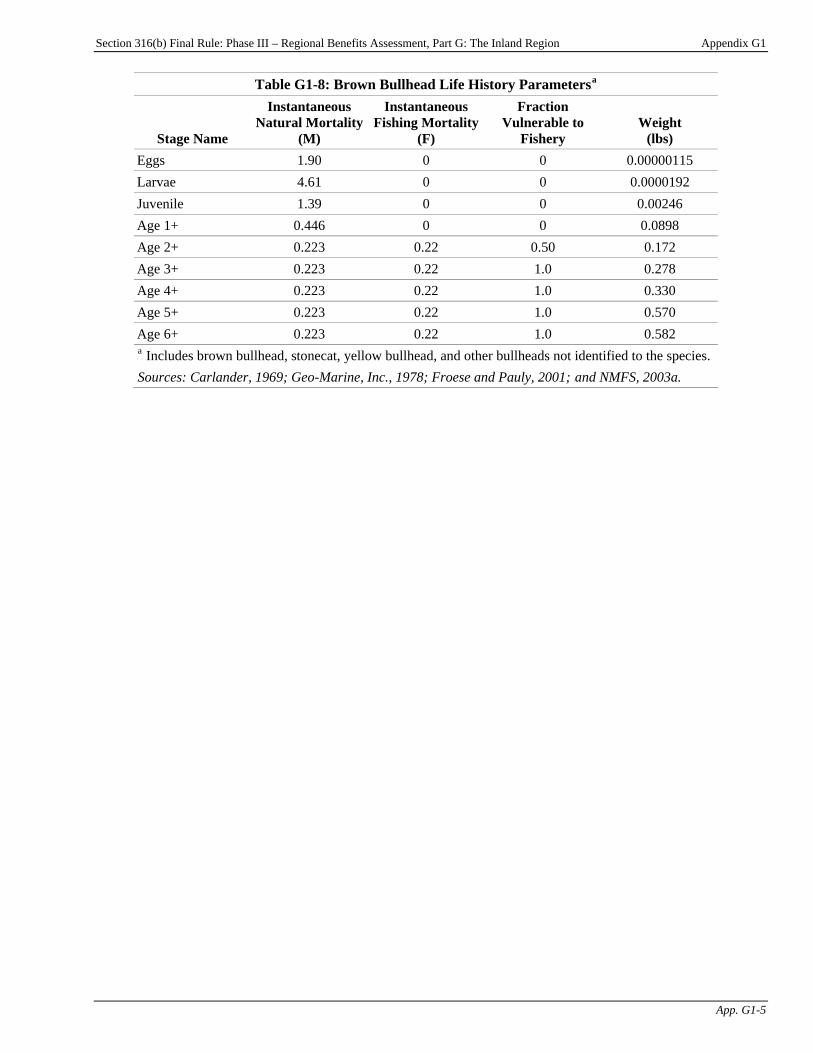
Section 316(b) Final Rule: Phase III – Regional Benefits Assessment, Part G: The Inland Region Appendix G1
App. G1-5
Table G1-8: Brown Bullhead Life History ParametersP
aP
Stage Name
Instantaneous Natural Mortality
(M)
Instantaneous Fishing Mortality
(F)
Fraction Vulnerable to
Fishery Weight
(lbs) Eggs 1.90 0 0 0.00000115 Larvae 4.61 0 0 0.0000192 Juvenile 1.39 0 0 0.00246 Age 1+ 0.446 0 0 0.0898 Age 2+ 0.223 0.22 0.50 0.172 Age 3+ 0.223 0.22 1.0 0.278 Age 4+ 0.223 0.22 1.0 0.330 Age 5+ 0.223 0.22 1.0 0.570 Age 6+ 0.223 0.22 1.0 0.582 P
aP Includes brown bullhead, stonecat, yellow bullhead, and other bullheads not identified to the species.
TSources: Carlander, 1969; Geo-Marine, Inc., 1978; Froese and Pauly, 2001; Tand NMFS, 2003a.
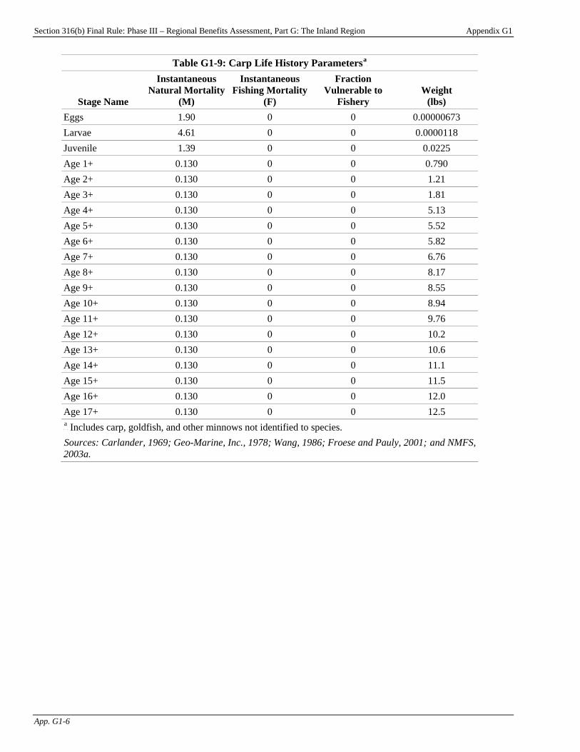
Section 316(b) Final Rule: Phase III – Regional Benefits Assessment, Part G: The Inland Region Appendix G1
App. G1-6
Table G1-9: Carp Life History ParametersP
aP
Stage Name
Instantaneous Natural Mortality
(M)
Instantaneous Fishing Mortality
(F)
Fraction Vulnerable to
Fishery Weight
(lbs) Eggs 1.90 0 0 0.00000673 Larvae 4.61 0 0 0.0000118 Juvenile 1.39 0 0 0.0225 Age 1+ 0.130 0 0 0.790 Age 2+ 0.130 0 0 1.21 Age 3+ 0.130 0 0 1.81 Age 4+ 0.130 0 0 5.13 Age 5+ 0.130 0 0 5.52 Age 6+ 0.130 0 0 5.82 Age 7+ 0.130 0 0 6.76 Age 8+ 0.130 0 0 8.17 Age 9+ 0.130 0 0 8.55 Age 10+ 0.130 0 0 8.94 Age 11+ 0.130 0 0 9.76 Age 12+ 0.130 0 0 10.2 Age 13+ 0.130 0 0 10.6 Age 14+ 0.130 0 0 11.1 Age 15+ 0.130 0 0 11.5 Age 16+ 0.130 0 0 12.0 Age 17+ 0.130 0 0 12.5 P
aP Includes carp, goldfish, and other minnows not identified to species.
TSources: Carlander, 1969; Geo-Marine, Inc., 1978; Wang, 1986; Froese and Pauly, 2001; Tand NMFS, 2003a.
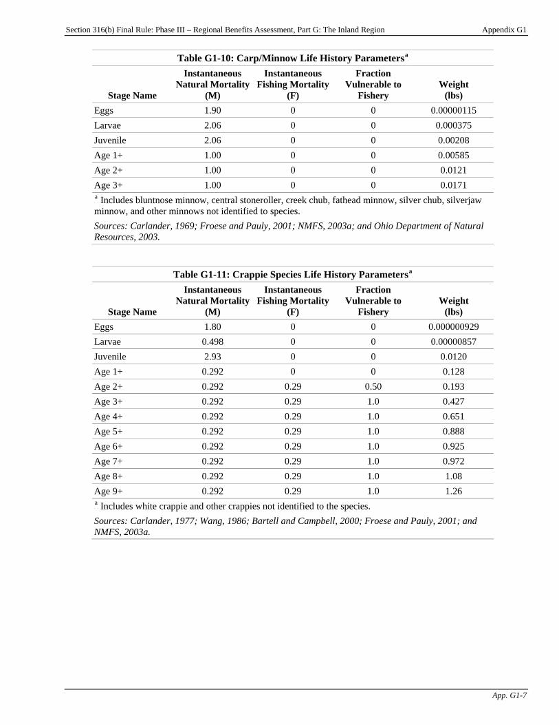
Section 316(b) Final Rule: Phase III – Regional Benefits Assessment, Part G: The Inland Region Appendix G1
App. G1-7
Table G1-10: Carp/Minnow Life History ParametersP
aP
Stage Name
Instantaneous Natural Mortality
(M)
Instantaneous Fishing Mortality
(F)
Fraction Vulnerable to
Fishery Weight
(lbs) Eggs 1.90 0 0 0.00000115 Larvae 2.06 0 0 0.000375 Juvenile 2.06 0 0 0.00208 Age 1+ 1.00 0 0 0.00585 Age 2+ 1.00 0 0 0.0121 Age 3+ 1.00 0 0 0.0171 P
aP Includes bluntnose minnow, central stoneroller, creek chub, fathead minnow, silver chub, silverjaw
minnow, and other minnows not identified to species.
Sources: Carlander, 1969; Froese and Pauly, 2001; NMFS, 2003a; and Ohio Department of Natural Resources, 2003.
Table G1-11: Crappie Species Life History ParametersP
aP
Stage Name
Instantaneous Natural Mortality
(M)
Instantaneous Fishing Mortality
(F)
Fraction Vulnerable to
Fishery Weight
(lbs) Eggs 1.80 0 0 0.000000929 Larvae 0.498 0 0 0.00000857 Juvenile 2.93 0 0 0.0120 Age 1+ 0.292 0 0 0.128 Age 2+ 0.292 0.29 0.50 0.193 Age 3+ 0.292 0.29 1.0 0.427 Age 4+ 0.292 0.29 1.0 0.651 Age 5+ 0.292 0.29 1.0 0.888 Age 6+ 0.292 0.29 1.0 0.925 Age 7+ 0.292 0.29 1.0 0.972 Age 8+ 0.292 0.29 1.0 1.08 Age 9+ 0.292 0.29 1.0 1.26 P
aP Includes white crappie and other crappies not identified to the species.
Sources: Carlander, 1977; Wang, 1986; Bartell and Campbell, 2000; Froese and Pauly, 2001; and NMFS, 2003a.
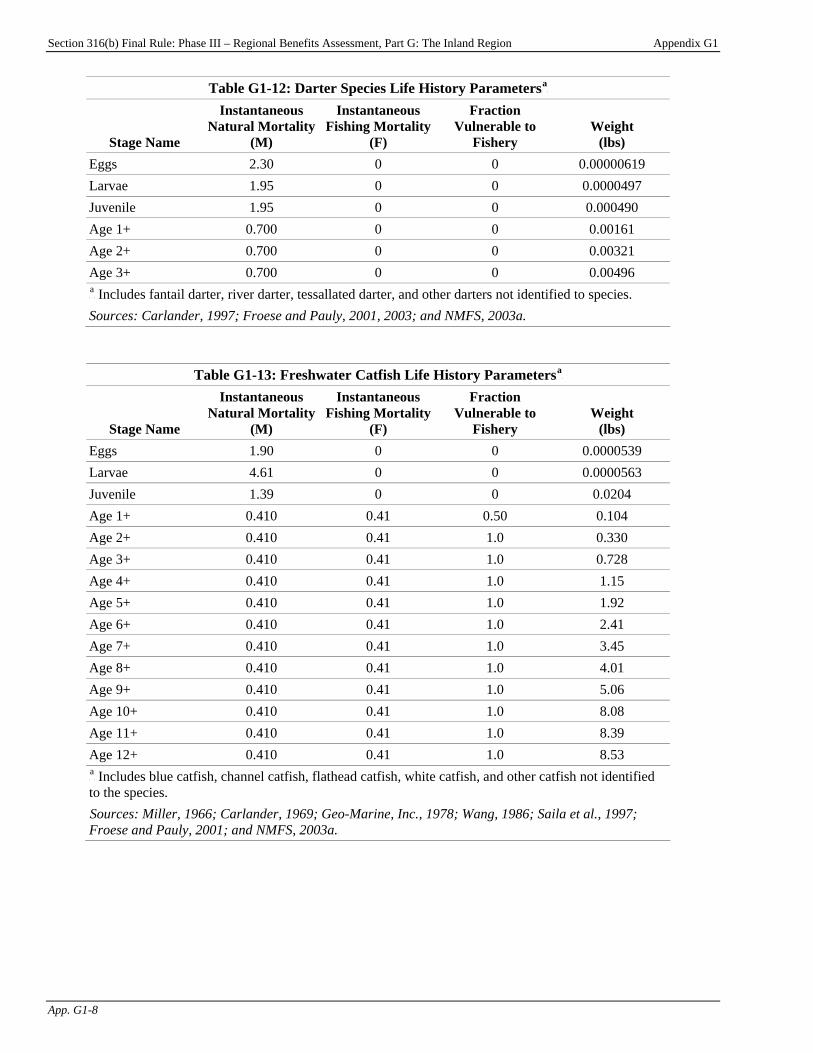
Section 316(b) Final Rule: Phase III – Regional Benefits Assessment, Part G: The Inland Region Appendix G1
App. G1-8
Table G1-12: Darter Species Life History ParametersP
aP
Stage Name
Instantaneous Natural Mortality
(M)
Instantaneous Fishing Mortality
(F)
Fraction Vulnerable to
Fishery Weight
(lbs) Eggs 2.30 0 0 0.00000619 Larvae 1.95 0 0 0.0000497 Juvenile 1.95 0 0 0.000490 Age 1+ 0.700 0 0 0.00161 Age 2+ 0.700 0 0 0.00321 Age 3+ 0.700 0 0 0.00496 P
aP Includes fantail darter, river darter, tessallated darter, and other darters not identified to species.
Sources: Carlander, 1997; Froese and Pauly, 2001, 2003; and NMFS, 2003a.
Table G1-13: Freshwater Catfish Life History ParametersP
aP
Stage Name
Instantaneous Natural Mortality
(M)
Instantaneous Fishing Mortality
(F)
Fraction Vulnerable to
Fishery Weight
(lbs) Eggs 1.90 0 0 0.0000539 Larvae 4.61 0 0 0.0000563 Juvenile 1.39 0 0 0.0204 Age 1+ 0.410 0.41 0.50 0.104 Age 2+ 0.410 0.41 1.0 0.330 Age 3+ 0.410 0.41 1.0 0.728 Age 4+ 0.410 0.41 1.0 1.15 Age 5+ 0.410 0.41 1.0 1.92 Age 6+ 0.410 0.41 1.0 2.41 Age 7+ 0.410 0.41 1.0 3.45 Age 8+ 0.410 0.41 1.0 4.01 Age 9+ 0.410 0.41 1.0 5.06 Age 10+ 0.410 0.41 1.0 8.08 Age 11+ 0.410 0.41 1.0 8.39 Age 12+ 0.410 0.41 1.0 8.53 P
aP Includes blue catfish, channel catfish, flathead catfish, white catfish, and other catfish not identified
to the species. TSources: Miller, 1966; Carlander, 1969; Geo-Marine, Inc., 1978; Wang, 1986; Saila et al., 1997; Froese and Pauly, 2001; and NMFS, 2003a.T
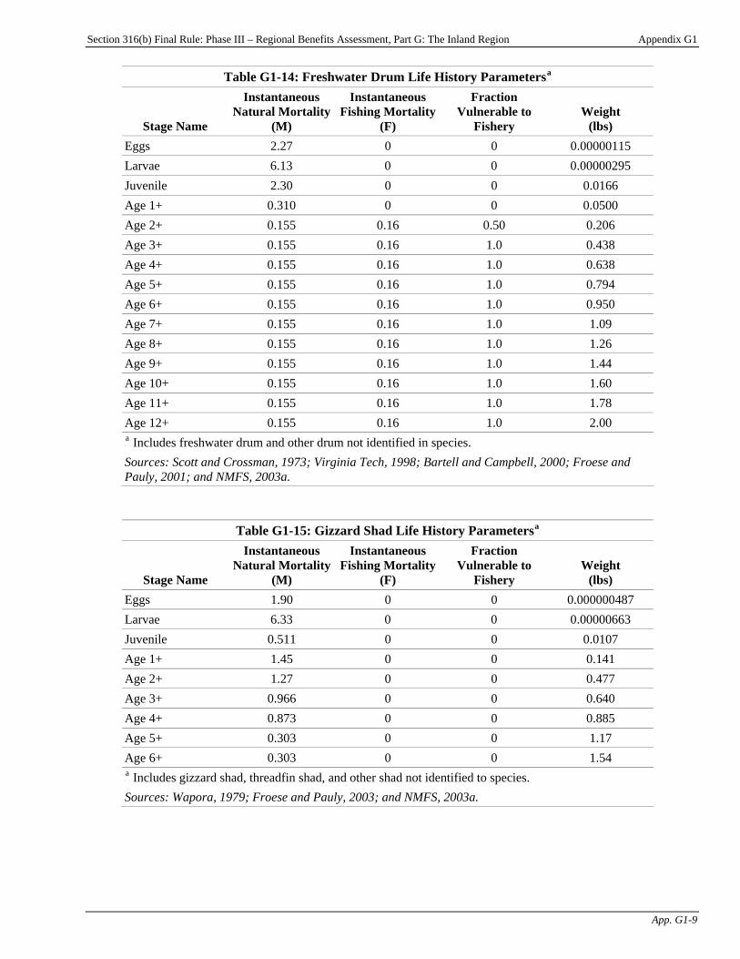
Section 316(b) Final Rule: Phase III – Regional Benefits Assessment, Part G: The Inland Region Appendix G1
App. G1-9
Table G1-14: Freshwater Drum Life History ParametersP
aP
Stage Name
Instantaneous Natural Mortality
(M)
Instantaneous Fishing Mortality
(F)
Fraction Vulnerable to
Fishery Weight
(lbs) Eggs 2.27 0 0 0.00000115 Larvae 6.13 0 0 0.00000295 Juvenile 2.30 0 0 0.0166 Age 1+ 0.310 0 0 0.0500 Age 2+ 0.155 0.16 0.50 0.206 Age 3+ 0.155 0.16 1.0 0.438 Age 4+ 0.155 0.16 1.0 0.638 Age 5+ 0.155 0.16 1.0 0.794 Age 6+ 0.155 0.16 1.0 0.950 Age 7+ 0.155 0.16 1.0 1.09 Age 8+ 0.155 0.16 1.0 1.26 Age 9+ 0.155 0.16 1.0 1.44 Age 10+ 0.155 0.16 1.0 1.60 Age 11+ 0.155 0.16 1.0 1.78 Age 12+ 0.155 0.16 1.0 2.00 P
aP Includes freshwater drum and other drum not identified in species.
Sources: Scott and Crossman, 1973; Virginia Tech, 1998; Bartell and Campbell, 2000; Froese and Pauly, 2001; and NMFS, 2003a.
Table G1-15: Gizzard Shad Life History ParametersP
aP
Stage Name
Instantaneous Natural Mortality
(M)
Instantaneous Fishing Mortality
(F)
Fraction Vulnerable to
Fishery Weight
(lbs) Eggs 1.90 0 0 0.000000487 Larvae 6.33 0 0 0.00000663 Juvenile 0.511 0 0 0.0107 Age 1+ 1.45 0 0 0.141 Age 2+ 1.27 0 0 0.477 Age 3+ 0.966 0 0 0.640 Age 4+ 0.873 0 0 0.885 Age 5+ 0.303 0 0 1.17 Age 6+ 0.303 0 0 1.54 P
aP Includes gizzard shad, threadfin shad, and other shad not identified to species.
Sources: Wapora, 1979; Froese and Pauly, 2003; and NMFS, 2003a.
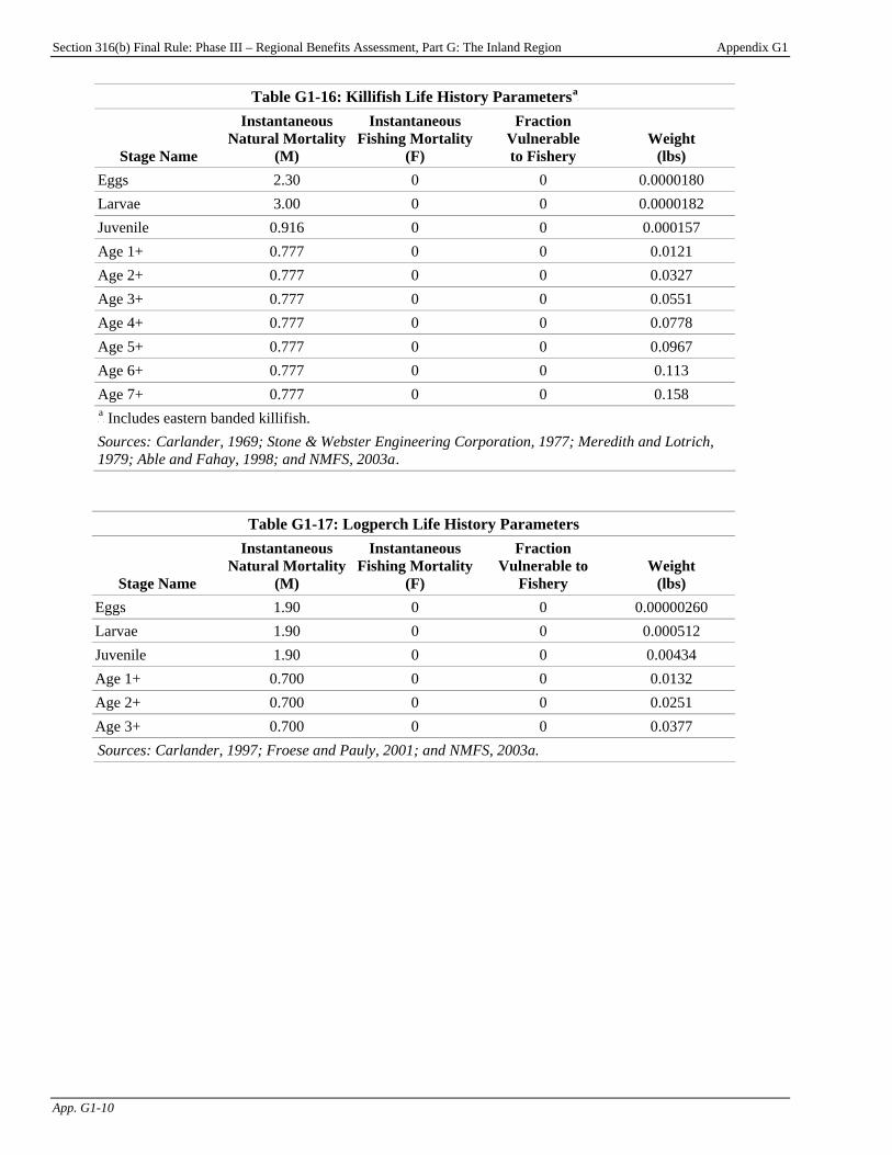
Section 316(b) Final Rule: Phase III – Regional Benefits Assessment, Part G: The Inland Region Appendix G1
App. G1-10
Table G1-16: Killifish Life History ParametersP
aP
Stage Name
Instantaneous Natural Mortality
(M)
Instantaneous Fishing Mortality
(F)
Fraction Vulnerable to Fishery
Weight (lbs)
Eggs 2.30 0 0 0.0000180 Larvae 3.00 0 0 0.0000182 Juvenile 0.916 0 0 0.000157 Age 1+ 0.777 0 0 0.0121 Age 2+ 0.777 0 0 0.0327 Age 3+ 0.777 0 0 0.0551 Age 4+ 0.777 0 0 0.0778 Age 5+ 0.777 0 0 0.0967 Age 6+ 0.777 0 0 0.113 Age 7+ 0.777 0 0 0.158 P
aP Includes eastern banded killifish.
Sources: TCarlander, 1969; Stone & Webster Engineering Corporation, 1977; Meredith and Lotrich, 1979; Able and Fahay, 1998; and NMFS, 2003aT.
Table G1-17: Logperch Life History Parameters
Stage Name
Instantaneous Natural Mortality
(M)
Instantaneous Fishing Mortality
(F)
Fraction Vulnerable to
Fishery Weight
(lbs) Eggs 1.90 0 0 0.00000260 Larvae 1.90 0 0 0.000512 Juvenile 1.90 0 0 0.00434 Age 1+ 0.700 0 0 0.0132 Age 2+ 0.700 0 0 0.0251 Age 3+ 0.700 0 0 0.0377 Sources: Carlander, 1997; Froese and Pauly, 2001; and NMFS, 2003a.
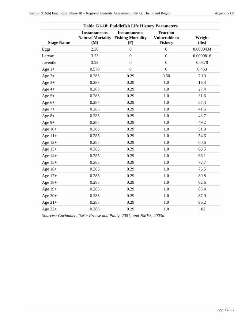
Section 316(b) Final Rule: Phase III – Regional Benefits Assessment, Part G: The Inland Region Appendix G1
App. G1-11
Table G1-18: Paddlefish Life History Parameters
Stage Name
Instantaneous Natural Mortality
(M)
Instantaneous Fishing Mortality
(F)
Fraction Vulnerable to
Fishery Weight
(lbs) Eggs 2.30 0 0 0.0000434 Larvae 3.23 0 0 0.0000816 Juvenile 3.23 0 0 0.0578 Age 1+ 0.570 0 0 0.453 Age 2+ 0.285 0.29 0.50 7.10 Age 3+ 0.285 0.29 1.0 16.3 Age 4+ 0.285 0.29 1.0 27.4 Age 5+ 0.285 0.29 1.0 31.6 Age 6+ 0.285 0.29 1.0 37.3 Age 7+ 0.285 0.29 1.0 41.6 Age 8+ 0.285 0.29 1.0 43.7 Age 9+ 0.285 0.29 1.0 49.2 Age 10+ 0.285 0.29 1.0 51.9 Age 11+ 0.285 0.29 1.0 54.6 Age 12+ 0.285 0.29 1.0 60.6 Age 13+ 0.285 0.29 1.0 63.5 Age 14+ 0.285 0.29 1.0 68.1 Age 15+ 0.285 0.29 1.0 72.7 Age 16+ 0.285 0.29 1.0 75.5 Age 17+ 0.285 0.29 1.0 80.8 Age 18+ 0.285 0.29 1.0 82.6 Age 19+ 0.285 0.29 1.0 85.4 Age 20+ 0.285 0.29 1.0 87.9 Age 21+ 0.285 0.29 1.0 96.2 Age 22+ 0.285 0.29 1.0 102 Sources: Carlander, 1969; Froese and Pauly, 2001; and NMFS, 2003a.
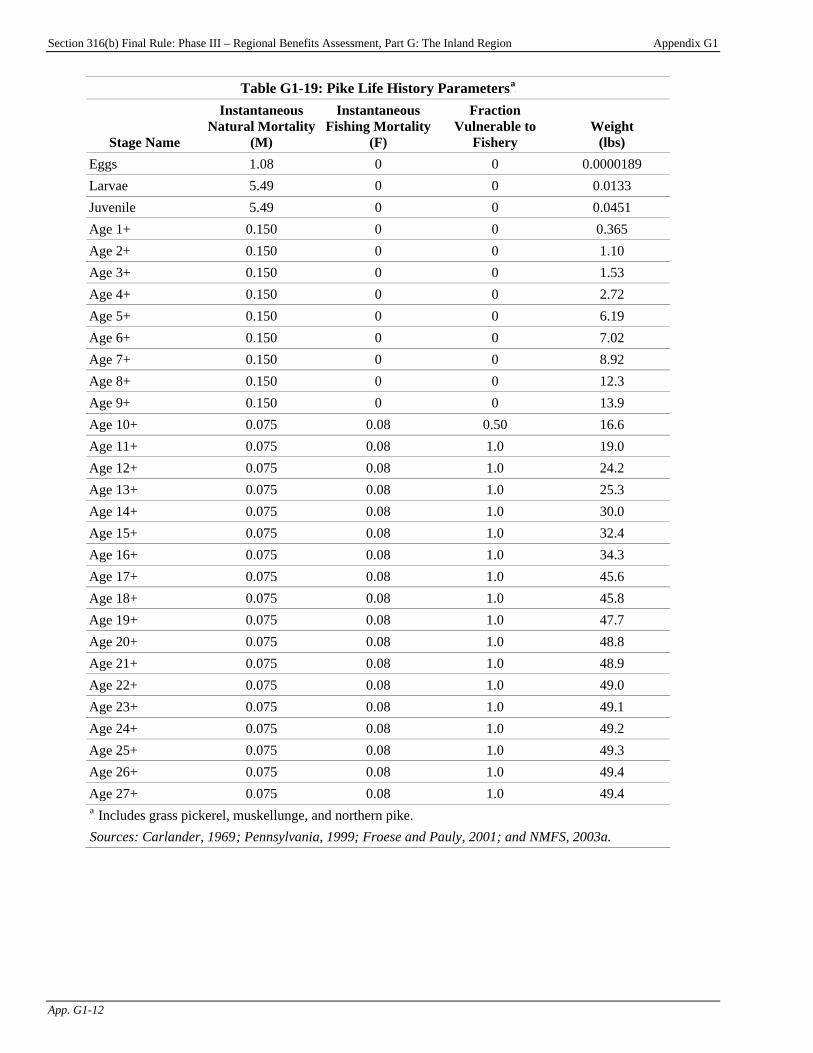
Section 316(b) Final Rule: Phase III – Regional Benefits Assessment, Part G: The Inland Region Appendix G1
App. G1-12
Table G1-19: Pike Life History ParametersP
aP
Stage Name
Instantaneous Natural Mortality
(M)
Instantaneous Fishing Mortality
(F)
Fraction Vulnerable to
Fishery Weight
(lbs) Eggs 1.08 0 0 0.0000189 Larvae 5.49 0 0 0.0133 Juvenile 5.49 0 0 0.0451 Age 1+ 0.150 0 0 0.365 Age 2+ 0.150 0 0 1.10 Age 3+ 0.150 0 0 1.53 Age 4+ 0.150 0 0 2.72 Age 5+ 0.150 0 0 6.19 Age 6+ 0.150 0 0 7.02 Age 7+ 0.150 0 0 8.92 Age 8+ 0.150 0 0 12.3 Age 9+ 0.150 0 0 13.9 Age 10+ 0.075 0.08 0.50 16.6 Age 11+ 0.075 0.08 1.0 19.0 Age 12+ 0.075 0.08 1.0 24.2 Age 13+ 0.075 0.08 1.0 25.3 Age 14+ 0.075 0.08 1.0 30.0 Age 15+ 0.075 0.08 1.0 32.4 Age 16+ 0.075 0.08 1.0 34.3 Age 17+ 0.075 0.08 1.0 45.6 Age 18+ 0.075 0.08 1.0 45.8 Age 19+ 0.075 0.08 1.0 47.7 Age 20+ 0.075 0.08 1.0 48.8 Age 21+ 0.075 0.08 1.0 48.9 Age 22+ 0.075 0.08 1.0 49.0 Age 23+ 0.075 0.08 1.0 49.1 Age 24+ 0.075 0.08 1.0 49.2 Age 25+ 0.075 0.08 1.0 49.3 Age 26+ 0.075 0.08 1.0 49.4 Age 27+ 0.075 0.08 1.0 49.4 P
aP Includes grass pickerel, muskellunge, and northern pike.
TSources: Carlander, 1969T; Pennsylvania, 1999; Froese and Pauly, 2001; and NMFS, 2003a.
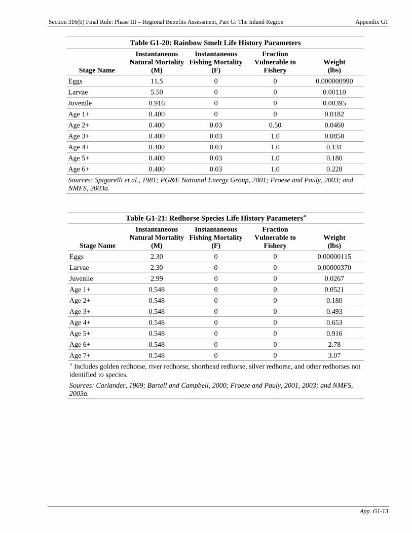
Section 316(b) Final Rule: Phase III – Regional Benefits Assessment, Part G: The Inland Region Appendix G1
App. G1-13
Table G1-20: Rainbow Smelt Life History Parameters
Stage Name
Instantaneous Natural Mortality
(M)
Instantaneous Fishing Mortality
(F)
Fraction Vulnerable to
Fishery Weight
(lbs) Eggs 11.5 0 0 0.000000990 Larvae 5.50 0 0 0.00110 Juvenile 0.916 0 0 0.00395 Age 1+ 0.400 0 0 0.0182 Age 2+ 0.400 0.03 0.50 0.0460 Age 3+ 0.400 0.03 1.0 0.0850 Age 4+ 0.400 0.03 1.0 0.131 Age 5+ 0.400 0.03 1.0 0.180 Age 6+ 0.400 0.03 1.0 0.228 Sources: Spigarelli et al., 1981; PG&E National Energy Group, 2001; Froese and Pauly, 2003; and NMFS, 2003a.
Table G1-21: Redhorse Species Life History ParametersP
aP
Stage Name
Instantaneous Natural Mortality
(M)
Instantaneous Fishing Mortality
(F)
Fraction Vulnerable to
Fishery Weight
(lbs) Eggs 2.30 0 0 0.00000115 Larvae 2.30 0 0 0.00000370 Juvenile 2.99 0 0 0.0267 Age 1+ 0.548 0 0 0.0521 Age 2+ 0.548 0 0 0.180 Age 3+ 0.548 0 0 0.493 Age 4+ 0.548 0 0 0.653 Age 5+ 0.548 0 0 0.916 Age 6+ 0.548 0 0 2.78 Age 7+ 0.548 0 0 3.07 P
aP Includes golden redhorse, river redhorse, shorthead redhorse, silver redhorse, and other redhorses not
identified to species. Sources: Carlander, 1969; Bartell and Campbell, 2000; Froese and Pauly, 2001, 2003; and NMFS, 2003a.
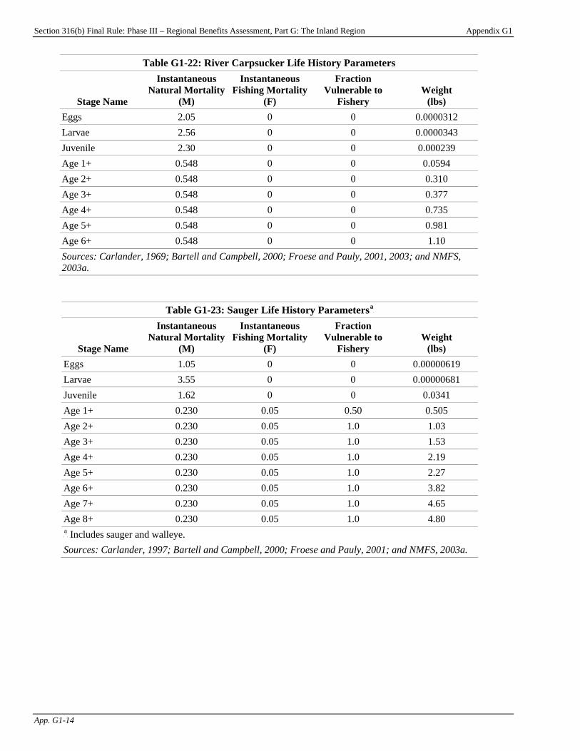
Section 316(b) Final Rule: Phase III – Regional Benefits Assessment, Part G: The Inland Region Appendix G1
App. G1-14
Table G1-22: River Carpsucker Life History Parameters
Stage Name
Instantaneous Natural Mortality
(M)
Instantaneous Fishing Mortality
(F)
Fraction Vulnerable to
Fishery Weight
(lbs) Eggs 2.05 0 0 0.0000312 Larvae 2.56 0 0 0.0000343 Juvenile 2.30 0 0 0.000239 Age 1+ 0.548 0 0 0.0594 Age 2+ 0.548 0 0 0.310 Age 3+ 0.548 0 0 0.377 Age 4+ 0.548 0 0 0.735 Age 5+ 0.548 0 0 0.981 Age 6+ 0.548 0 0 1.10 Sources: Carlander, 1969; Bartell and Campbell, 2000; Froese and Pauly, 2001, 2003; and NMFS, 2003a.
Table G1-23: Sauger Life History ParametersP
aP
Stage Name
Instantaneous Natural Mortality
(M)
Instantaneous Fishing Mortality
(F)
Fraction Vulnerable to
Fishery Weight
(lbs) Eggs 1.05 0 0 0.00000619 Larvae 3.55 0 0 0.00000681 Juvenile 1.62 0 0 0.0341 Age 1+ 0.230 0.05 0.50 0.505 Age 2+ 0.230 0.05 1.0 1.03 Age 3+ 0.230 0.05 1.0 1.53 Age 4+ 0.230 0.05 1.0 2.19 Age 5+ 0.230 0.05 1.0 2.27 Age 6+ 0.230 0.05 1.0 3.82 Age 7+ 0.230 0.05 1.0 4.65 Age 8+ 0.230 0.05 1.0 4.80 P
aP Includes sauger and walleye.
Sources: Carlander, 1997; Bartell and Campbell, 2000; Froese and Pauly, 2001; and NMFS, 2003a.
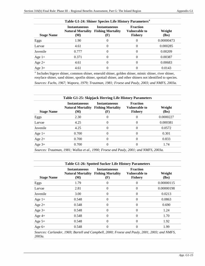
Section 316(b) Final Rule: Phase III – Regional Benefits Assessment, Part G: The Inland Region Appendix G1
App. G1-15
Table G1-24: Shiner Species Life History ParametersP
aP
Stage Name
Instantaneous Natural Mortality
(M)
Instantaneous Fishing Mortality
(F)
Fraction Vulnerable to
Fishery Weight
(lbs) Eggs 1.90 0 0 0.00000473 Larvae 4.61 0 0 0.000285 Juvenile 0.777 0 0 0.00209 Age 1+ 0.371 0 0 0.00387 Age 2+ 4.61 0 0 0.00683 Age 3+ 4.61 0 0 0.0143 P
aP Includes bigeye shiner, common shiner, emerald shiner, golden shiner, mimic shiner, river shiner,
rosyface shiner, sand shiner, spotfin shiner, spottail shiner, and other shiners not identified to species. Sources: Fuchs, 1967; Wapora, 1979; Trautman, 1981; Froese and Pauly, 2003; and NMFS, 2003a.
Table G1-25: Skipjack Herring Life History Parameters
Stage Name
Instantaneous Natural Mortality
(M)
Instantaneous Fishing Mortality
(F)
Fraction Vulnerable to
Fishery Weight
(lbs) Eggs 2.30 0 0 0.0000227 Larvae 4.25 0 0 0.000381 Juvenile 4.25 0 0 0.0572 Age 1+ 0.700 0 0 0.301 Age 2+ 0.700 0 0 0.833 Age 3+ 0.700 0 0 1.74 Sources: Trautman, 1981; Wallus et al., 1990; Froese and Pauly, 2001; and NMFS, 2003a.
Table G1-26: Spotted Sucker Life History Parameters
Stage Name
Instantaneous Natural Mortality
(M)
Instantaneous Fishing Mortality
(F)
Fraction Vulnerable to
Fishery Weight
(lbs) Eggs 1.79 0 0 0.00000115 Larvae 2.81 0 0 0.00000198 Juvenile 3.00 0 0 0.0213 Age 1+ 0.548 0 0 0.0863 Age 2+ 0.548 0 0 0.690 Age 3+ 0.548 0 0 1.24 Age 4+ 0.548 0 0 1.70 Age 5+ 0.548 0 0 1.92 Age 6+ 0.548 0 0 1.99 Sources: Carlander, 1969; Bartell and Campbell, 2000; Froese and Pauly, 2001, 2003; and NMFS, 2003a.
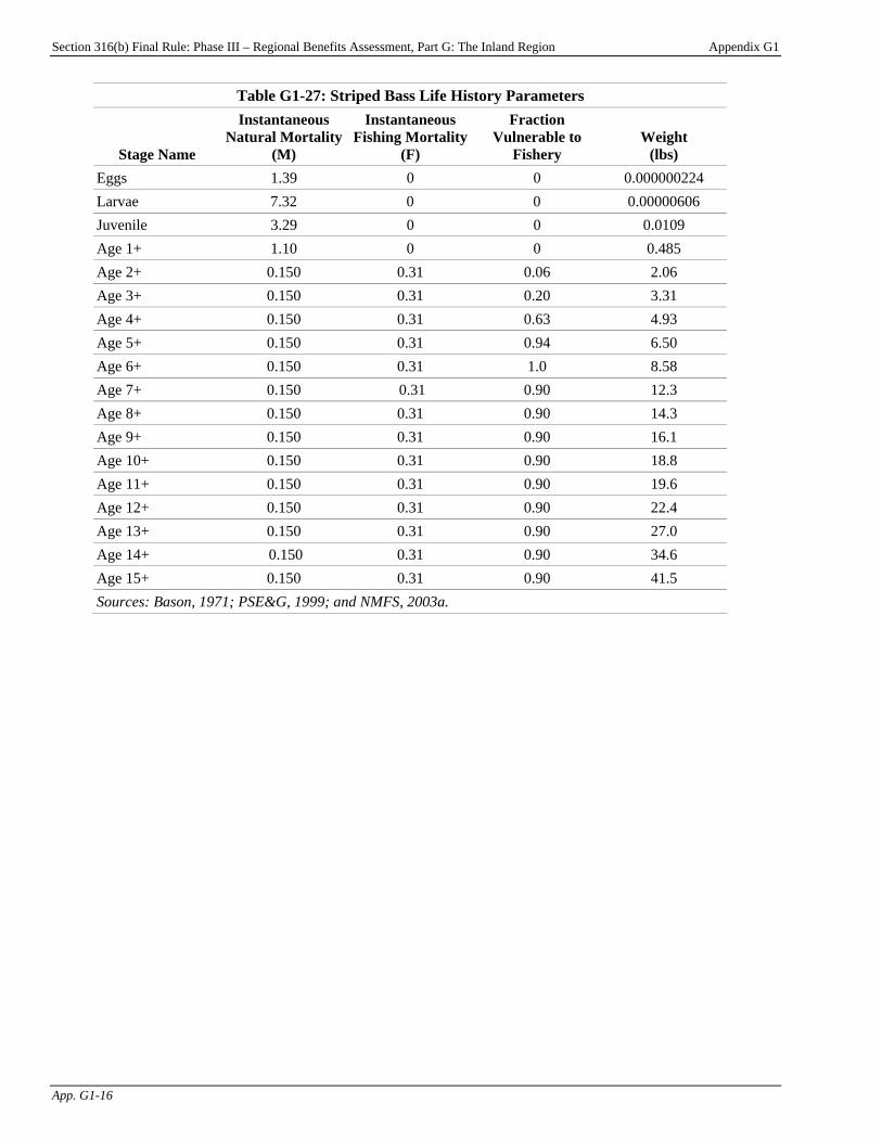
Section 316(b) Final Rule: Phase III – Regional Benefits Assessment, Part G: The Inland Region Appendix G1
App. G1-16
Table G1-27: Striped Bass Life History Parameters
Stage Name
Instantaneous Natural Mortality
(M)
Instantaneous Fishing Mortality
(F)
Fraction Vulnerable to
Fishery Weight
(lbs) Eggs 1.39 0 0 0.000000224 Larvae 7.32 0 0 0.00000606 Juvenile 3.29 0 0 0.0109 Age 1+ 1.10 0 0 0.485 Age 2+ 0.150 0.31 0.06 2.06 Age 3+ 0.150 0.31 0.20 3.31 Age 4+ 0.150 0.31 0.63 4.93 Age 5+ 0.150 0.31 0.94 6.50 Age 6+ 0.150 0.31 1.0 8.58 Age 7+ 0.150 0.31 0.90 12.3 Age 8+ 0.150 0.31 0.90 14.3 Age 9+ 0.150 0.31 0.90 16.1 Age 10+ 0.150 0.31 0.90 18.8 Age 11+ 0.150 0.31 0.90 19.6 Age 12+ 0.150 0.31 0.90 22.4 Age 13+ 0.150 0.31 0.90 27.0 Age 14+ 0.150 0.31 0.90 34.6 Age 15+ 0.150 0.31 0.90 41.5 Sources: Bason, 1971; PSE&G, 1999; and NMFS, 2003a.
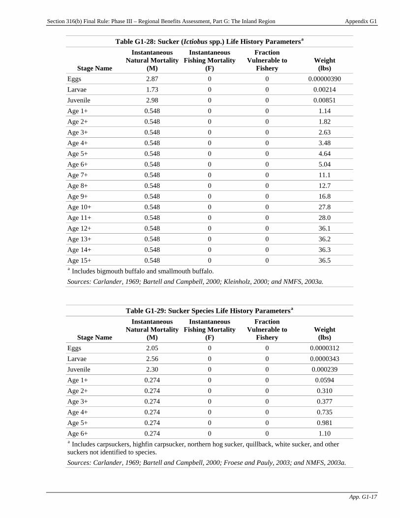
Section 316(b) Final Rule: Phase III – Regional Benefits Assessment, Part G: The Inland Region Appendix G1
App. G1-17
Table G1-28: Sucker (Ictiobus spp.) Life History ParametersP
aP
Stage Name
Instantaneous Natural Mortality
(M)
Instantaneous Fishing Mortality
(F)
Fraction Vulnerable to
Fishery Weight
(lbs) Eggs 2.87 0 0 0.00000390 Larvae 1.73 0 0 0.00214 Juvenile 2.98 0 0 0.00851 Age 1+ 0.548 0 0 1.14 Age 2+ 0.548 0 0 1.82 Age 3+ 0.548 0 0 2.63 Age 4+ 0.548 0 0 3.48 Age 5+ 0.548 0 0 4.64 Age 6+ 0.548 0 0 5.04 Age 7+ 0.548 0 0 11.1 Age 8+ 0.548 0 0 12.7 Age 9+ 0.548 0 0 16.8 Age 10+ 0.548 0 0 27.8 Age 11+ 0.548 0 0 28.0 Age 12+ 0.548 0 0 36.1 Age 13+ 0.548 0 0 36.2 Age 14+ 0.548 0 0 36.3 Age 15+ 0.548 0 0 36.5 P
aP Includes bigmouth buffalo and smallmouth buffalo.
Sources: Carlander, 1969; Bartell and Campbell, 2000; Kleinholz, 2000; and NMFS, 2003a.
Table G1-29: Sucker Species Life History ParametersP
aP
Stage Name
Instantaneous Natural Mortality
(M)
Instantaneous Fishing Mortality
(F)
Fraction Vulnerable to
Fishery Weight
(lbs) Eggs 2.05 0 0 0.0000312 Larvae 2.56 0 0 0.0000343 Juvenile 2.30 0 0 0.000239 Age 1+ 0.274 0 0 0.0594 Age 2+ 0.274 0 0 0.310 Age 3+ 0.274 0 0 0.377 Age 4+ 0.274 0 0 0.735 Age 5+ 0.274 0 0 0.981 Age 6+ 0.274 0 0 1.10 P
aP Includes carpsuckers, highfin carpsucker, northern hog sucker, quillback, white sucker, and other
suckers not identified to species. Sources: Carlander, 1969; Bartell and Campbell, 2000; Froese and Pauly, 2003; and NMFS, 2003a.
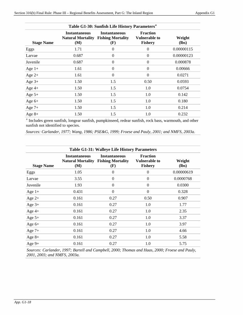
Section 316(b) Final Rule: Phase III – Regional Benefits Assessment, Part G: The Inland Region Appendix G1
App. G1-18
Table G1-30: Sunfish Life History ParametersP
aP
Stage Name
Instantaneous Natural Mortality
(M)
Instantaneous Fishing Mortality
(F)
Fraction Vulnerable to
Fishery Weight
(lbs) Eggs 1.71 0 0 0.00000115 Larvae 0.687 0 0 0.00000123 Juvenile 0.687 0 0 0.000878 Age 1+ 1.61 0 0 0.00666 Age 2+ 1.61 0 0 0.0271 Age 3+ 1.50 1.5 0.50 0.0593 Age 4+ 1.50 1.5 1.0 0.0754 Age 5+ 1.50 1.5 1.0 0.142 Age 6+ 1.50 1.5 1.0 0.180 Age 7+ 1.50 1.5 1.0 0.214 Age 8+ 1.50 1.5 1.0 0.232 P
aP Includes green sunfish, longear sunfish, pumpkinseed, redear sunfish, rock bass, warmouth, and other
sunfish not identified to species. Sources: Carlander, 1977; Wang, 1986; PSE&G, 1999; Froese and Pauly, 2001; and NMFS, 2003a.
Table G1-31: Walleye Life History Parameters
Stage Name
Instantaneous Natural Mortality
(M)
Instantaneous Fishing Mortality
(F)
Fraction Vulnerable to
Fishery Weight
(lbs) Eggs 1.05 0 0 0.00000619 Larvae 3.55 0 0 0.0000768 Juvenile 1.93 0 0 0.0300 Age 1+ 0.431 0 0 0.328 Age 2+ 0.161 0.27 0.50 0.907 Age 3+ 0.161 0.27 1.0 1.77 Age 4+ 0.161 0.27 1.0 2.35 Age 5+ 0.161 0.27 1.0 3.37 Age 6+ 0.161 0.27 1.0 3.97 Age 7+ 0.161 0.27 1.0 4.66 Age 8+ 0.161 0.27 1.0 5.58 Age 9+ 0.161 0.27 1.0 5.75 Sources: TCarlander, 1997;T Bartell and Campbell, 2000; Thomas and Haas, 2000; Froese and Pauly, 2001, 2003; and NMFS, 2003a.
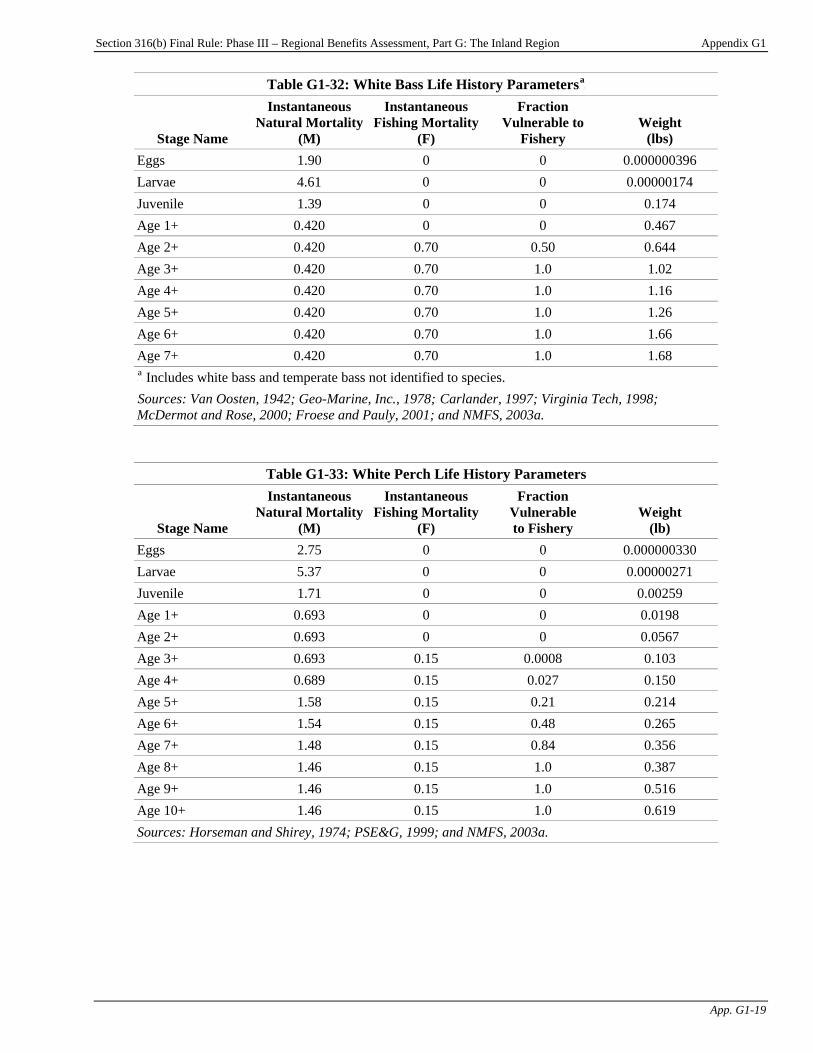
Section 316(b) Final Rule: Phase III – Regional Benefits Assessment, Part G: The Inland Region Appendix G1
App. G1-19
Table G1-32: White Bass Life History ParametersP
aP
Stage Name
Instantaneous Natural Mortality
(M)
Instantaneous Fishing Mortality
(F)
Fraction Vulnerable to
Fishery Weight
(lbs) Eggs 1.90 0 0 0.000000396 Larvae 4.61 0 0 0.00000174 Juvenile 1.39 0 0 0.174 Age 1+ 0.420 0 0 0.467 Age 2+ 0.420 0.70 0.50 0.644 Age 3+ 0.420 0.70 1.0 1.02 Age 4+ 0.420 0.70 1.0 1.16 Age 5+ 0.420 0.70 1.0 1.26 Age 6+ 0.420 0.70 1.0 1.66 Age 7+ 0.420 0.70 1.0 1.68 P
aP Includes white bass and temperate bass not identified to species.
TSources: Van Oosten, 1942; Geo-Marine, Inc., 1978;T Carlander, 1997; Virginia Tech, 1998; McDermot and Rose, 2000; Froese and Pauly, 2001; and NMFS, 2003a.
Table G1-33: White Perch Life History Parameters
Stage Name
Instantaneous Natural Mortality
(M)
Instantaneous Fishing Mortality
(F)
Fraction Vulnerable to Fishery
Weight (lb)
Eggs 2.75 0 0 0.000000330 Larvae 5.37 0 0 0.00000271 Juvenile 1.71 0 0 0.00259 Age 1+ 0.693 0 0 0.0198 Age 2+ 0.693 0 0 0.0567 Age 3+ 0.693 0.15 0.0008 0.103 Age 4+ 0.689 0.15 0.027 0.150 Age 5+ 1.58 0.15 0.21 0.214 Age 6+ 1.54 0.15 0.48 0.265 Age 7+ 1.48 0.15 0.84 0.356 Age 8+ 1.46 0.15 1.0 0.387 Age 9+ 1.46 0.15 1.0 0.516 Age 10+ 1.46 0.15 1.0 0.619 Sources: Horseman and Shirey, 1974; PSE&G, 1999; and NMFS, 2003a.
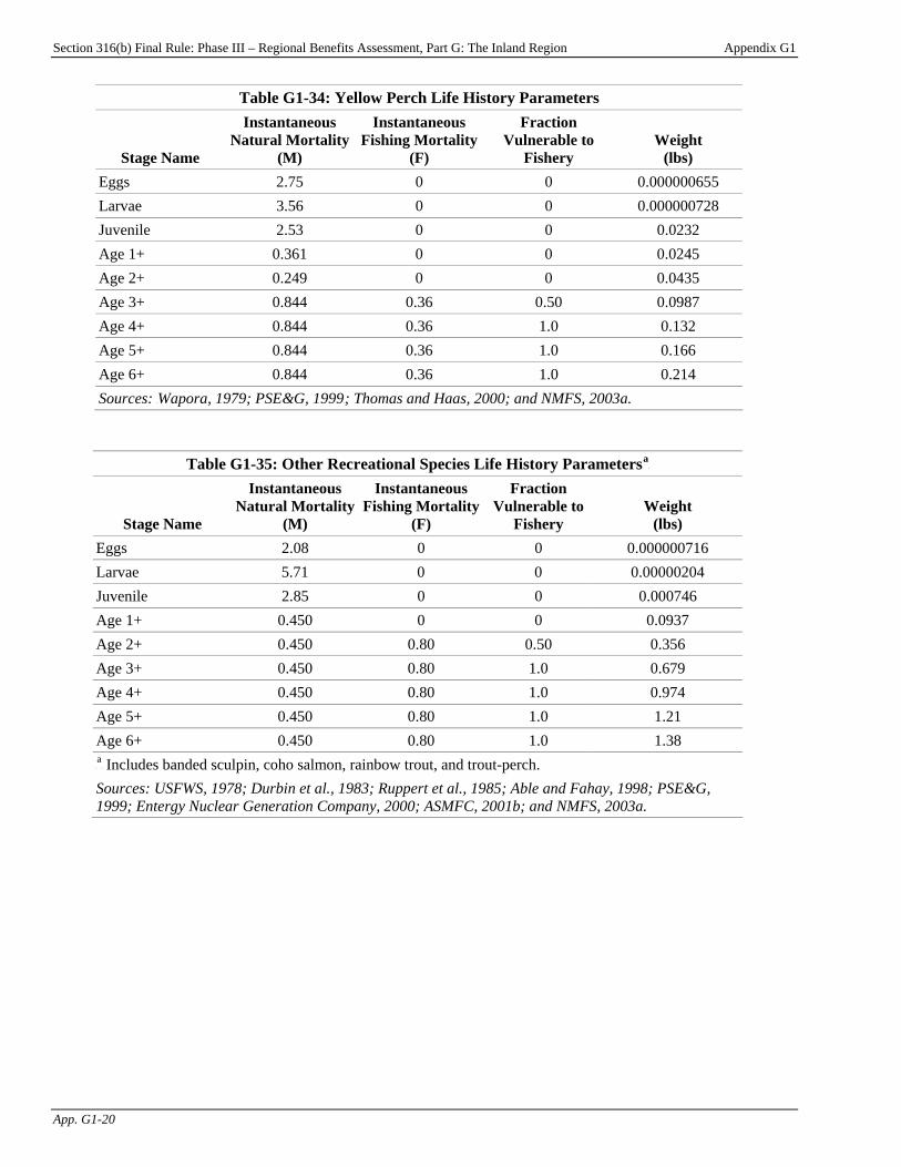
Section 316(b) Final Rule: Phase III – Regional Benefits Assessment, Part G: The Inland Region Appendix G1
App. G1-20
Table G1-34: Yellow Perch Life History Parameters
Stage Name
Instantaneous Natural Mortality
(M)
Instantaneous Fishing Mortality
(F)
Fraction Vulnerable to
Fishery Weight
(lbs) Eggs 2.75 0 0 0.000000655 Larvae 3.56 0 0 0.000000728 Juvenile 2.53 0 0 0.0232 Age 1+ 0.361 0 0 0.0245 Age 2+ 0.249 0 0 0.0435 Age 3+ 0.844 0.36 0.50 0.0987 Age 4+ 0.844 0.36 1.0 0.132 Age 5+ 0.844 0.36 1.0 0.166 Age 6+ 0.844 0.36 1.0 0.214 Sources: TWapora, 1979; PSE&G, 1999T; Thomas and Haas, 2000; and NMFS, 2003a.
Table G1-35: Other Recreational Species Life History ParametersP
aP
Stage Name
Instantaneous Natural Mortality
(M)
Instantaneous Fishing Mortality
(F)
Fraction Vulnerable to
Fishery Weight
(lbs) Eggs 2.08 0 0 0.000000716 Larvae 5.71 0 0 0.00000204 Juvenile 2.85 0 0 0.000746 Age 1+ 0.450 0 0 0.0937 Age 2+ 0.450 0.80 0.50 0.356 Age 3+ 0.450 0.80 1.0 0.679 Age 4+ 0.450 0.80 1.0 0.974 Age 5+ 0.450 0.80 1.0 1.21 Age 6+ 0.450 0.80 1.0 1.38 P
aP Includes banded sculpin, coho salmon, rainbow trout, and trout-perch.
Sources: USFWS, 1978; Durbin et al., 1983; Ruppert et al., 1985; Able and Fahay, 1998; PSE&G, 1999; Entergy Nuclear Generation Company, 2000; ASMFC, 2001b; and NMFS, 2003a.

Section 316(b) Final Rule: Phase III – Regional Benefits Assessment, Part G: The Inland Region Appendix G1
App. G1-21
Table G1-36: Other Forage Species Life History ParametersP
aP
Stage Name
Instantaneous Natural Mortality
(M)
Instantaneous Fishing Mortality
(F)
Fraction Vulnerable to
Fishery Weight
(lbs) Eggs 1.04 0 0 0.0000000186 Larvae 7.70 0 0 0.00000158 Juvenile 1.29 0 0 0.000481 Age 1+ 1.62 0 0 0.00381 Age 2+ 1.62 0 0 0.00496 Age 3+ 1.62 0 0 0.00505 P
aP Includes American eel, chestnut lamprey, goldeye, longnose gar, madtoms, mooneye, silver lamprey,
and other forage fish not identified to species. Sources: Derickson and Price, 1973; and PSE&G, 1999.

Section 316(b) Proposed Rule: Phase III – Regional Benefits Assessment, Part G: The Inland Region Chapter G2
G2-1
Chapter G2: Evaluation of Impingement and Entrainment in the Inland Region
G2-1 I&E Species/Species Groups
Evaluated Table G2-1 provides a list of species/species groups that were evaluated in EPA’s analysis of impingement and entrainment (I&E) in the Inland region. There is not a significant level of commercial fishing in the interior U.S. Therefore, EPA has assumed that all I&E losses in this region affect recreational fisheries only.
Table G2-1: Species/Species Groups Evaluated by EPA that are Subject to I&E in the Inland Region
Species/Species Group Recreational Commercial Forage Alewife X American shad X Bay anchovy X Bigmouth buffalo X Black bullhead X Black crappie X Blue crab X Blueback herring X Bluegill X Bluntnose minnow X Brown bullhead X Bullhead species X Burbot X Carp X Channel catfish X Crappie X Darter species X Emerald shiner X Freshwater drum X Gizzard shad X Gobies X
Chapter Contents G2-1 I&E Species/Species Groups Evaluated ....... G2-1 G2-2 I&E Data Evaluated ...................................... G2-3 G2-3 EPA’s Estimate of Current I&E at Phase III Facilities in the Inland Region Expressed as Age-1 Equivalents and Foregone Yield ........ G2-4 G2-4 Reductions in I&E at Phase III Facilities in the Inland Region Under Alternative Options....................................... G2-7 G2-5 Assumptions Used in Calculating
Recreational and Commercial Losses ........... G2-7
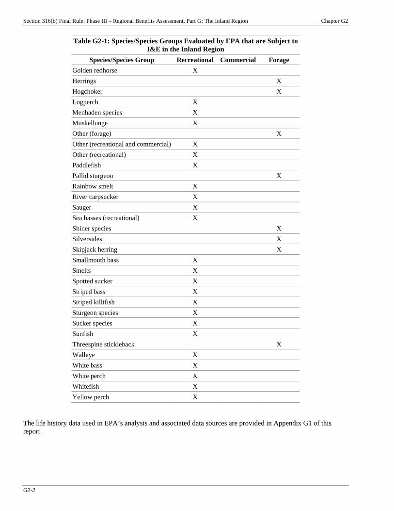
Section 316(b) Final Rule: Phase III – Regional Benefits Assessment, Part G: The Inland Region Chapter G2
G2-2
Table G2-1: Species/Species Groups Evaluated by EPA that are Subject to I&E in the Inland Region
Species/Species Group Recreational Commercial Forage Golden redhorse X Herrings X Hogchoker X Logperch X Menhaden species X Muskellunge X Other (forage) X Other (recreational and commercial) X Other (recreational) X Paddlefish X Pallid sturgeon X Rainbow smelt X River carpsucker X Sauger X Sea basses (recreational) X Shiner species X Silversides X Skipjack herring X Smallmouth bass X Smelts X Spotted sucker X Striped bass X Striped killifish X Sturgeon species X Sucker species X Sunfish X Threespine stickleback X Walleye X White bass X White perch X Whitefish X Yellow perch X
The life history data used in EPA’s analysis and associated data sources are provided in Appendix G1 of this report.
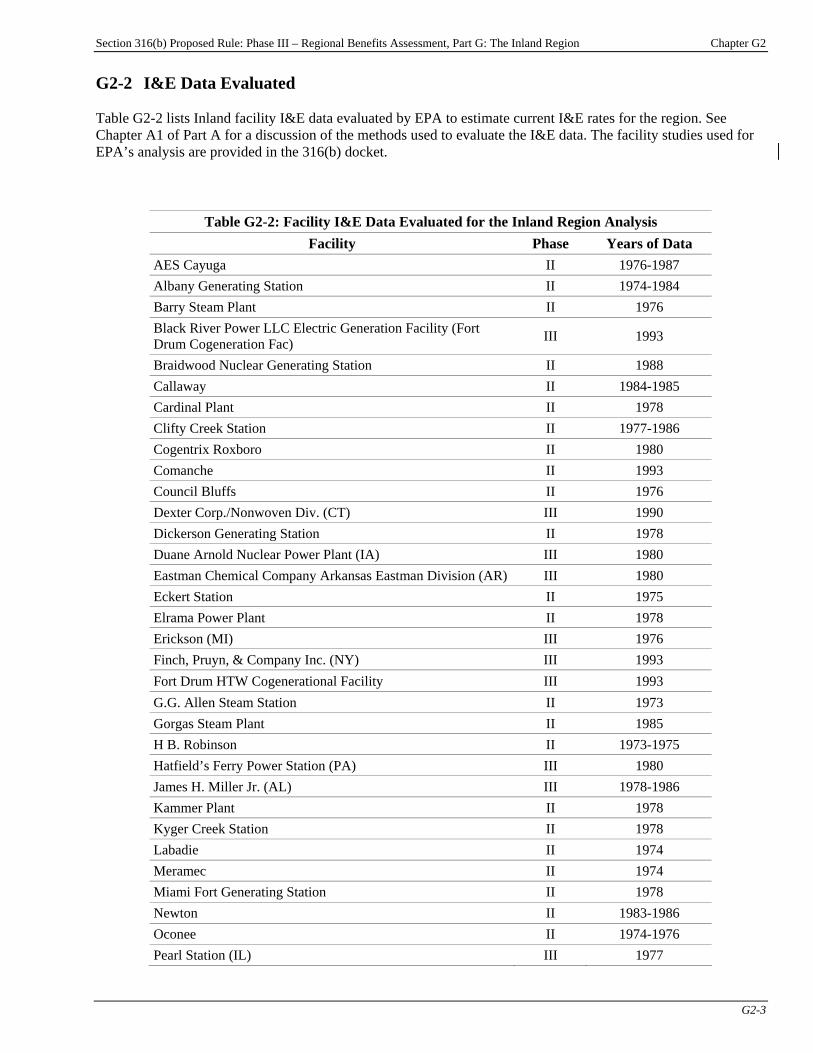
Section 316(b) Proposed Rule: Phase III – Regional Benefits Assessment, Part G: The Inland Region Chapter G2
G2-3
G2-2 I&E Data Evaluated Table G2-2 lists Inland facility I&E data evaluated by EPA to estimate current I&E rates for the region. See Chapter A1 of Part A for a discussion of the methods used to evaluate the I&E data. The facility studies used for EPA’s analysis are provided in the 316(b) docket.
Table G2-2: Facility I&E Data Evaluated for the Inland Region Analysis Facility Phase Years of Data
AES Cayuga II 1976-1987 Albany Generating Station II 1974-1984 Barry Steam Plant II 1976 Black River Power LLC Electric Generation Facility (Fort Drum Cogeneration Fac) III 1993
Braidwood Nuclear Generating Station II 1988 Callaway II 1984-1985 Cardinal Plant II 1978 Clifty Creek Station II 1977-1986 Cogentrix Roxboro II 1980 Comanche II 1993 Council Bluffs II 1976 Dexter Corp./Nonwoven Div. (CT) III 1990 Dickerson Generating Station II 1978 Duane Arnold Nuclear Power Plant (IA) III 1980 Eastman Chemical Company Arkansas Eastman Division (AR) III 1980 Eckert Station II 1975 Elrama Power Plant II 1978 Erickson (MI) III 1976 Finch, Pruyn, & Company Inc. (NY) III 1993 Fort Drum HTW Cogenerational Facility III 1993 G.G. Allen Steam Station II 1973 Gorgas Steam Plant II 1985 H B. Robinson II 1973-1975 Hatfield’s Ferry Power Station (PA) III 1980 James H. Miller Jr. (AL) III 1978-1986 Kammer Plant II 1978 Kyger Creek Station II 1978 Labadie II 1974 Meramec II 1974 Miami Fort Generating Station II 1978 Newton II 1983-1986 Oconee II 1974-1976 Pearl Station (IL) III 1977

Section 316(b) Final Rule: Phase III – Regional Benefits Assessment, Part G: The Inland Region Chapter G2
G2-4
Table G2-2: Facility I&E Data Evaluated for the Inland Region Analysis Facility Phase Years of Data
Philip Sporn Plant II 1978 Putnam III 1979 Seminole (FL) III 1979 Sherburne Co. (MN) III 1974-1975 Tanners Creek Plant II 1977 Three Mile Island II 1977 W.H. Sammis Generating Station II 1977 Wabash River Plant II 1976 Walter C. Beckjord Generating Station II 1977 Wateree Generating Station II 1976 Winyah Generating Station (SC) III 1981
G2-3 EPA’s Estimate of Current I&E at Phase III Facilities in the Inland Region
Expressed as Age-1 Equivalents and Foregone Yield Table G2-3 provides EPA’s estimate of the annual age-1 equivalents and foregone fishery yield resulting from the impingement of aquatic species at facilities located in the Inland region. Table G2-4 displays this information for entrainment. Note that in these tables, “total yield” includes direct losses of harvested species and the yield of harvested species that is lost due to losses of forage species (trophic transfer). As discussed in Chapter A1 of Part A of the section 316(b) Phase III Regional Benefits Assessment, the conversion of forage to yield contributes only a very small fraction to total yield.
Table G2-3: Estimated Current Annual Impingement at Phase III Facilities in the Inland Region Expressed as Age-1 Equivalents and Foregone Fishery Yield
Species/Species Group Age-1 Equivalents
(#s) Total Yield
(lbs) Alewife 37,800 <1 American shad 7,030 1,730 Bay anchovy 2,880 <1 Bigmouth buffalo 873 <1 Black bullhead 1,120 88 Black crappie 1,990 335 Blue crab <1 <1 Blueback herring 251,000 <1 Bluegill 285,000 5,520 Bluntnose minnow 6,350 <1 Brown bullhead 7,460 615 Bullhead species 8,980 736 Burbot 45 <1 Carp 14,400 <1 Channel catfish 219,000 45,400 Crappie 15,100 2,550
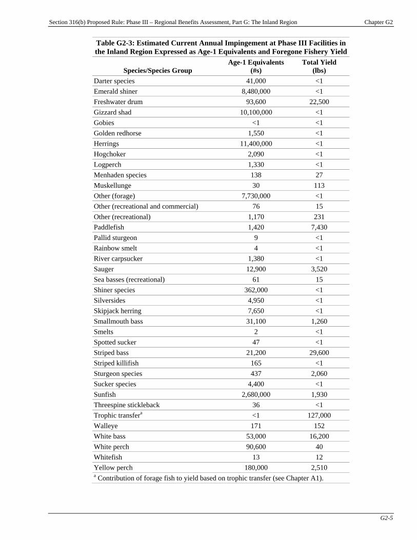
Section 316(b) Proposed Rule: Phase III – Regional Benefits Assessment, Part G: The Inland Region Chapter G2
G2-5
Table G2-3: Estimated Current Annual Impingement at Phase III Facilities in the Inland Region Expressed as Age-1 Equivalents and Foregone Fishery Yield
Species/Species Group Age-1 Equivalents
(#s) Total Yield
(lbs) Darter species 41,000 <1 Emerald shiner 8,480,000 <1 Freshwater drum 93,600 22,500 Gizzard shad 10,100,000 <1 Gobies <1 <1 Golden redhorse 1,550 <1 Herrings 11,400,000 <1 Hogchoker 2,090 <1 Logperch 1,330 <1 Menhaden species 138 27 Muskellunge 30 113 Other (forage) 7,730,000 <1 Other (recreational and commercial) 76 15 Other (recreational) 1,170 231 Paddlefish 1,420 7,430 Pallid sturgeon 9 <1 Rainbow smelt 4 <1 River carpsucker 1,380 <1 Sauger 12,900 3,520 Sea basses (recreational) 61 15 Shiner species 362,000 <1 Silversides 4,950 <1 Skipjack herring 7,650 <1 Smallmouth bass 31,100 1,260 Smelts 2 <1 Spotted sucker 47 <1 Striped bass 21,200 29,600 Striped killifish 165 <1 Sturgeon species 437 2,060 Sucker species 4,400 <1 Sunfish 2,680,000 1,930 Threespine stickleback 36 <1 Trophic transfera <1 127,000 Walleye 171 152 White bass 53,000 16,200 White perch 90,600 40 Whitefish 13 12 Yellow perch 180,000 2,510 a Contribution of forage fish to yield based on trophic transfer (see Chapter A1).
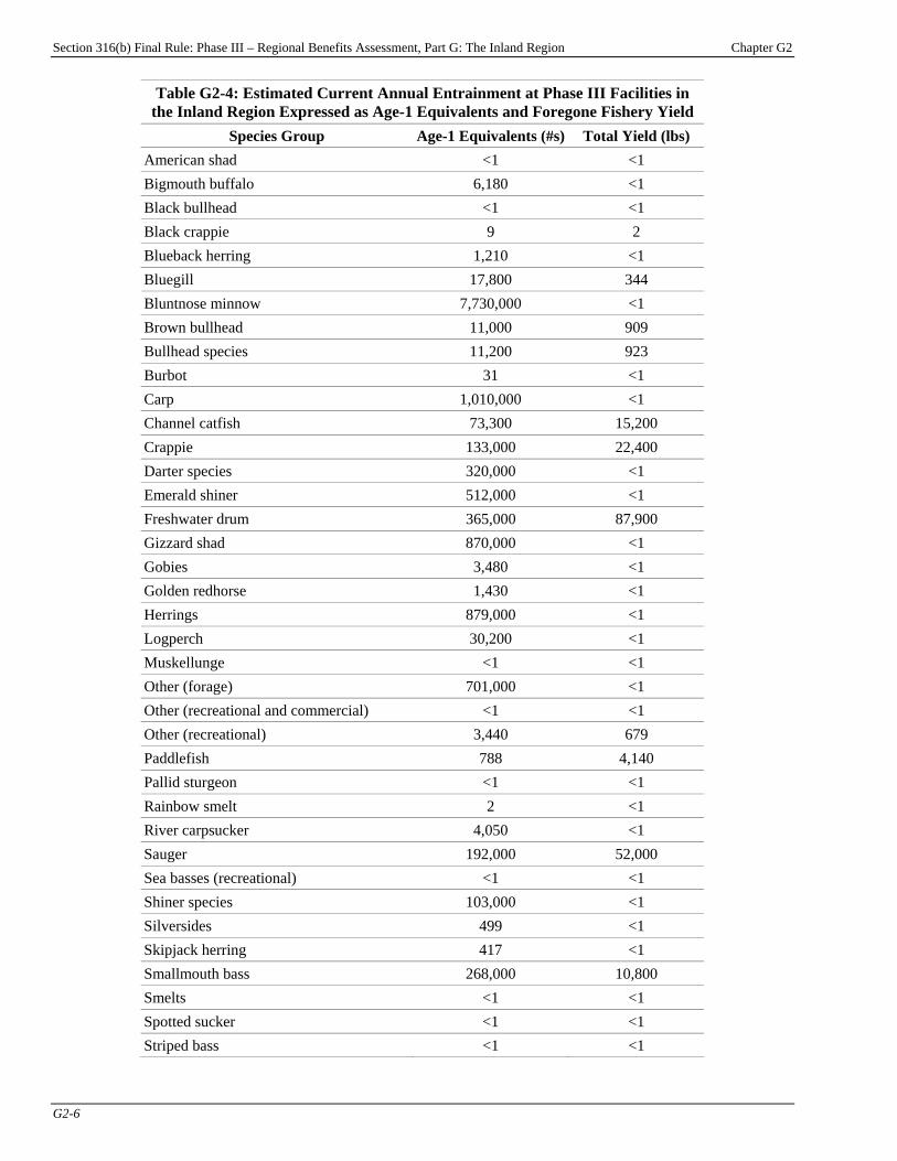
Section 316(b) Final Rule: Phase III – Regional Benefits Assessment, Part G: The Inland Region Chapter G2
G2-6
Table G2-4: Estimated Current Annual Entrainment at Phase III Facilities in the Inland Region Expressed as Age-1 Equivalents and Foregone Fishery Yield
Species Group Age-1 Equivalents (#s) Total Yield (lbs) American shad <1 <1 Bigmouth buffalo 6,180 <1 Black bullhead <1 <1 Black crappie 9 2 Blueback herring 1,210 <1 Bluegill 17,800 344 Bluntnose minnow 7,730,000 <1 Brown bullhead 11,000 909 Bullhead species 11,200 923 Burbot 31 <1 Carp 1,010,000 <1 Channel catfish 73,300 15,200 Crappie 133,000 22,400 Darter species 320,000 <1 Emerald shiner 512,000 <1 Freshwater drum 365,000 87,900 Gizzard shad 870,000 <1 Gobies 3,480 <1 Golden redhorse 1,430 <1 Herrings 879,000 <1 Logperch 30,200 <1 Muskellunge <1 <1 Other (forage) 701,000 <1 Other (recreational and commercial) <1 <1 Other (recreational) 3,440 679 Paddlefish 788 4,140 Pallid sturgeon <1 <1 Rainbow smelt 2 <1 River carpsucker 4,050 <1 Sauger 192,000 52,000 Sea basses (recreational) <1 <1 Shiner species 103,000 <1 Silversides 499 <1 Skipjack herring 417 <1 Smallmouth bass 268,000 10,800 Smelts <1 <1 Spotted sucker <1 <1 Striped bass <1 <1
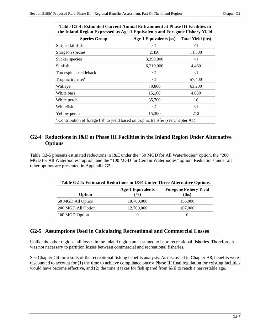
Section 316(b) Proposed Rule: Phase III – Regional Benefits Assessment, Part G: The Inland Region Chapter G2
G2-7
Table G2-4: Estimated Current Annual Entrainment at Phase III Facilities in the Inland Region Expressed as Age-1 Equivalents and Foregone Fishery Yield
Species Group Age-1 Equivalents (#s) Total Yield (lbs) Striped killifish <1 <1 Sturgeon species 2,450 11,500 Sucker species 3,390,000 <1 Sunfish 6,210,000 4,480 Threespine stickleback <1 <1 Trophic transfera <1 57,400 Walleye 70,800 63,200 White bass 15,100 4,630 White perch 35,700 16 Whitefish <1 <1 Yellow perch 15,300 212 a Contribution of forage fish to yield based on trophic transfer (see Chapter A1).
G2-4 Reductions in I&E at Phase III Facilities in the Inland Region Under Alternative
Options Table G2-5 presents estimated reductions in I&E under the “50 MGD for All Waterbodies” option, the “200 MGD for All Waterbodies” option, and the “100 MGD for Certain Waterbodies” option. Reductions under all other options are presented in Appendix G2.
Table G2-5: Estimated Reductions in I&E Under Three Alternative Options
Option Age-1 Equivalents
(#s) Foregone Fishery Yield
(lbs) 50 MGD All Option 19,700,000 155,000 200 MGD All Option 12,700,000 107,000 100 MGD Option 0 0
G2-5 Assumptions Used in Calculating Recreational and Commercial Losses Unlike the other regions, all losses in the Inland region are assumed to be to recreational fisheries. Therefore, it was not necessary to partition losses between commercial and recreational fisheries. See Chapter G4 for results of the recreational fishing benefits analysis. As discussed in Chapter A8, benefits were discounted to account for (1) the time to achieve compliance once a Phase III final regulation for existing facilities would have become effective, and (2) the time it takes for fish spared from I&E to reach a harvestable age.

Section 316(b) Final Rule: Phase III – Regional Benefits Assessment, Part G: The Inland Region Appendix G2
App. G2-1
Appendix G2: Reductions in I&E Under Supplemental Policy Options
Table G2-1: Estimated Reductions in I&E in the Inland Region Under Eight Supplemental Options
Option Age-1 Equivalents
(#s) Foregone Fishery Yield
(lbs) Electric Generators 2-50 MGD
I-only Everywhere 473,000 3,050 I&E like Phase II 509,000 3,590 I&E Everywhere 802,000 7,870
Manufacturers 2-50 MGD I-only Everywhere 3,320,000 21,400 I&E like Phase II 3,660,000 26,500 I&E Everywhere 4,880,000 44,300
Manufacturers 50+ MGD I-only Everywhere 16,200,000 105,000 I&E Everywhere 24,600,000 228,000

Section 316(b) Final Rule: Phase III – Regional Benefits Assessment, Part G: The Inland Region Chapter G3
G3-1
Chapter G3: Commercial Fishing Benefits There is no significant level of commercial fishing in the interior United States. Therefore, EPA has assumed that all impingement and entrainment losses in this region affect recreational fisheries only. As a result, commercial fishing losses and benefits for the Inland region are assumed to be $0.
Section 316(b) Final Rule: Phase III – Regional Benefits Assessment, Part G: The Inland Region Appendix G3
App. G3-1
Appendix G3: Commercial Fishing Benefits Under Supplemental Policy Options
There is no significant level of commercial fishing in the interior United States. Therefore, EPA has assumed that all impingement and entrainment losses in this region affect recreational fisheries only. As a result, baseline commercial fishing losses and benefits for the Inland region are assumed to be $0. For additional information on the options, please see the TDD.
Section 316(b) Final Rule: Phase III – Regional Benefits Assessment, Part G: The Inland Region Chapter G4
G4-1
Chapter G4: Recreational Use Benefits
Chapter Contents G4-1 Benefit Transfer Approach Based on Meta-Analysis............................................... G4-1 G4-1.1 Baseline Losses and Reductions in Recreational Fishery Losses Under the Regulatory Options ................... G4-2 G4-1.2 Recreational Fishing Benefits from Eliminating Baseline I&E Losses ............................................. G4-3 G4-1.3 Recreational Fishing Benefits of the “50 MGD for All Waterbodies” Option ............................................. G4-4 G4-1.4 Recreational Fishing Benefits of the “200 MGD for All Waterbodies” Option ...................... G4-5 G4-1.5 Recreational Fishing Benefits of the “100 MGD for Certain Waterbodies” Option ...................... G4-6 G4-2 Limitations and Uncertainty ......................... G4-6
Introduction This chapter presents the results of the recreational fishing benefits analysis for the Inland region. The chapter presents EPA’s estimates of baseline (i.e., current) annual recreational fishery losses from impingement and entrainment (I&E) at potentially regulated facilities in the Inland region and annual reductions in these losses under the regulatory options for Phase III existing facilitiesPF
1FP:
< the “50 MGD for All Waterbodies” option, < the “200 MGD for All Waterbodies” option,
and < the “100 MGD for Certain Waterbodies”
option. The chapter then presents the estimated welfare gain to Inland anglers from eliminating baseline recreational fishing losses from I&E and the expected benefits under the regulatory options. EPA estimated the recreational benefits of reducing and eliminating I&E losses using a benefit transfer methodology based on a meta-analysis of the marginal value of catching different species of fish. This meta-analysis is discussed in detail in Chapter A5, “Recreational Fishing Benefits Methodology.” EPA considered a wide range of policy options in developing this regulation. In addition to the regulatory options, EPA evaluated various supplemental options. For additional information on the options, please see the TDD. Appendix G4 presents results of the recreational fishing benefits analysis for the supplemental options. G4-1 Benefit Transfer Approach Based on Meta-Analysis EPA estimated the recreational welfare gain from the reduction in annual I&E losses expected under the policy options, and the welfare gain from eliminating I&E at potentially regulated facilities, using a benefit transfer approach. As discussed in Chapter A5, the Agency used a meta-analysis regression equation to estimate the marginal recreational value per additional fish caught by anglers, for different species in different regions. Since I&E at potentially regulated facilities affects a variety of species, EPA assigned each species with I&E losses to one of the general species groups used in the meta-analysis. The Agency then calculated the economic value of reducing or eliminating baseline I&E losses, for each species group, by multiplying the value per fish for that species group by the number of fish in the group that are lost in the baseline or saved under the policy options.PF
2FP
In general, the fit between the species with I&E losses and the species groups in the meta-analysis was good. However, EPA’s estimates of baseline I&E losses and reductions in I&E under the policy options included losses
P
1P See the Introduction to this report for a description of the regulatory options.
P
2P The estimates of I&E presented in this chapter include only the fraction of impinged and entrained recreational
fish that would be caught by anglers. The total amount of I&E of recreational species is actually much higher.
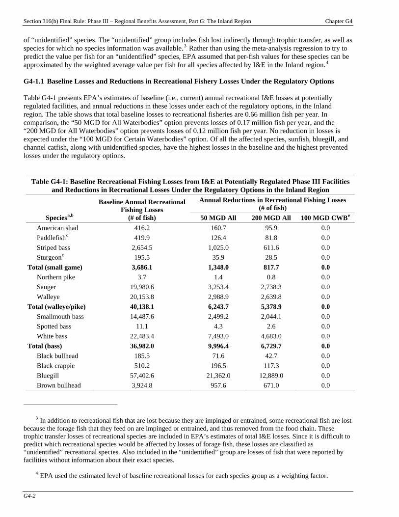
Section 316(b) Final Rule: Phase III – Regional Benefits Assessment, Part G: The Inland Region Chapter G4
G4-2
of “unidentified” species. The “unidentified” group includes fish lost indirectly through trophic transfer, as well as species for which no species information was available.PF
3FP Rather than using the meta-analysis regression to try to
predict the value per fish for an “unidentified” species, EPA assumed that per-fish values for these species can be approximated by the weighted average value per fish for all species affected by I&E in the Inland region.PF
4FP
G4-1.1 Baseline Losses and Reductions in Recreational Fishery Losses Under the Regulatory Options Table G4-1 presents EPA’s estimates of baseline (i.e., current) annual recreational I&E losses at potentially regulated facilities, and annual reductions in these losses under each of the regulatory options, in the Inland region. The table shows that total baseline losses to recreational fisheries are 0.66 million fish per year. In comparison, the “50 MGD for All Waterbodies” option prevents losses of 0.17 million fish per year, and the “200 MGD for All Waterbodies” option prevents losses of 0.12 million fish per year. No reduction in losses is expected under the “100 MGD for Certain Waterbodies” option. Of all the affected species, sunfish, bluegill, and channel catfish, along with unidentified species, have the highest losses in the baseline and the highest prevented losses under the regulatory options.
Table G4-1: Baseline Recreational Fishing Losses from I&E at Potentially Regulated Phase III Facilities and Reductions in Recreational Losses Under the Regulatory Options in the Inland Region
Annual Reductions in Recreational Fishing Losses (# of fish)
SpeciesP
a,bP
Baseline Annual Recreational Fishing Losses
(# of fish) 50 MGD All 200 MGD All 100 MGD CWBP
eP
American shad 416.2 160.7 95.9 0.0 PaddlefishP
cP 419.9 126.4 81.8 0.0
Striped bass 2,654.5 1,025.0 611.6 0.0 SturgeonP
cP 195.5 35.9 28.5 0.0
Total (small game) 3,686.1 1,348.0 817.7 0.0 Northern pike 3.7 1.4 0.8 0.0 Sauger 19,980.6 3,253.4 2,738.3 0.0 Walleye 20,153.8 2,988.9 2,639.8 0.0
Total (walleye/pike) 40,138.1 6,243.7 5,378.9 0.0 Smallmouth bass 14,487.6 2,499.2 2,044.1 0.0 Spotted bass 11.1 4.3 2.6 0.0 White bass 22,483.4 7,493.0 4,683.0 0.0
Total (bass) 36,982.0 9,996.4 6,729.7 0.0 Black bullhead 185.5 71.6 42.7 0.0 Black crappie 510.2 196.5 117.3 0.0 Bluegill 57,402.6 21,362.0 12,889.0 0.0 Brown bullhead 3,924.8 957.6 671.0 0.0
P
3P In addition to recreational fish that are lost because they are impinged or entrained, some recreational fish are lost
because the forage fish that they feed on are impinged or entrained, and thus removed from the food chain. These trophic transfer losses of recreational species are included in EPA’s estimates of total I&E losses. Since it is difficult to predict which recreational species would be affected by losses of forage fish, these losses are classified as “unidentified” recreational species. Also included in the “unidentified” group are losses of fish that were reported by facilities without information about their exact species.
P
4P EPA used the estimated level of baseline recreational losses for each species group as a weighting factor.

Section 316(b) Final Rule: Phase III – Regional Benefits Assessment, Part G: The Inland Region Chapter G4
G4-3
Table G4-1: Baseline Recreational Fishing Losses from I&E at Potentially Regulated Phase III Facilities and Reductions in Recreational Losses Under the Regulatory Options in the Inland Region
Annual Reductions in Recreational Fishing Losses (# of fish)
SpeciesP
a,bP
Baseline Annual Recreational Fishing Losses
(# of fish) 50 MGD All 200 MGD All 100 MGD CWBP
eP
Bullhead 3,478.7 881.8 608.6 0.0 Channel catfish 48,922.1 15,964.5 10,047.9 0.0 Crappie 37,849.4 6,514.1 5,334.0 0.0 Menhaden 41.7 16.1 9.6 0.0 Sunfish 103,406.3 22,703.7 16,623.7 0.0 White perch 239.6 76.4 48.5 0.0 Yellow perch 21,591.0 7,935.0 4,806.2 0.0
Total (panfish) 277,552.2 76,679.5 51,198.7 0.0 WhitefishP
dP 8.0 3.1 1.8 0.0
Total (trout) 8.0 3.1 1.8 0.0 Total (unidentified) 299,651.3 80,260.7 54,220.2 0.0 Total (all species) 658,017.6 174,531.4 118,347.0 0.0 P
aP EPA assigned each species with I&E losses to one of the species groups used in the meta-analysis. The
“unidentified” group includes fish lost indirectly through trophic transfer, fish reported lost without information about their species, and freshwater drum. Freshwater drum were included in this group because there were no valuation studies available and this species does not correspond well with any of the other species groups. P
bP This table includes several species of anadromous fish (such as American shad and striped bass) that are classified in
saltwater species groups, but that are commonly caught in freshwater during part of their life cycle. P
cP No valuation studies were available for freshwater sturgeon or paddlefish. EPA included these two species in the
“small game” group because the typical size of these species is consistent with (or larger than) the size of other species in the “small game” group. Adult lake sturgeon generally weigh 10 to 80 pounds and measure three to five feet in length, and may grow as large as 300 pounds and seven feet long (NYSDEC, 2003). White sturgeon, which are anadromous, can grow to 400 pounds or 10 feet in length (Monterey Bay Aquarium, 1999). Paddlefish are also very large, averaging between 3.3 and 4.8 feet in length (Jenkins and Burkhead, 1993). P
dP EPA included whitefish in the “trout” category because its physical characteristics are similar to trout, and lake
whitefish are prized for their meat. Therefore, valuing them in the panfish category would be inappropriate. P
eP No facilities in the Inland region would be regulated under the “100 MGD for Certain Waterbodies” option, so no
benefits are expected in this region under this option. Source: U.S. EPA analysis for this report.
G4-1.2 Recreational Fishing Benefits from Eliminating Baseline I&E Losses Table G4-2 shows the results of EPA’s analysis of the welfare gain to recreational anglers from eliminating baseline recreational fishery losses at potentially regulated facilities in the Inland region. The table presents baseline annual recreational I&E losses, the estimated value per fish, and the monetized annual welfare gain from eliminating recreational losses, for each species group. Total baseline recreational fishing losses for the Inland region are 658.0 thousand fish per year. The undiscounted annual welfare gain to Inland anglers from eliminating these losses is $1.25 million (2004$), with lower and upper bounds of $0.69 million and $2.26 million. Evaluated at 3% and 7% discount rates, the mean annualized welfare gain of eliminating these losses is $1.21 million and $1.16 million, respectively. The majority of monetized recreational losses from I&E under baseline conditions are attributable to losses of freshwater drum (categorized in the “unidentified” group) and other “unidentified” species.
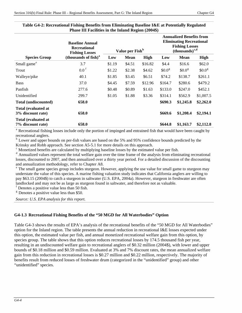
Section 316(b) Final Rule: Phase III – Regional Benefits Assessment, Part G: The Inland Region Chapter G4
G4-4
Table G4-2: Recreational Fishing Benefits from Eliminating Baseline I&E at Potentially Regulated Phase III Facilities in the Inland Region (2004$)
Value per FishP
bP
Annualized Benefits from Eliminating Recreational
Fishing Losses (thousands)P
c,dP
Species Group
Baseline Annual Recreational
Fishing Losses (thousands of fish)P
aP Low Mean High Low Mean High
Small gameP
eP 3.7 $1.19 $4.51 $16.82 $4.4 $16.6 $62.0
Trout 0.0P
fP $1.22 $2.38 $4.62 $0.0P
gP $0.0P
gP $0.0P
gP
Walleye/pike 40.1 $1.85 $3.45 $6.51 $74.2 $138.7 $261.1 Bass 37.0 $4.45 $7.59 $12.96 $164.7 $280.6 $479.2 Panfish 277.6 $0.48 $0.89 $1.63 $133.0 $247.0 $452.1 Unidentified 299.7 $1.05 $1.88 $3.36 $314.1 $562.9 $1,007.5 Total (undiscounted) 658.0 $690.3 $1,245.8 $2,262.0 Total (evaluated at 3% discount rate) 658.0 $669.6 $1,208.4 $2,194.1 Total (evaluated at 7% discount rate) 658.0 $644.8 $1,163.7 $2,112.8 P
aP Recreational fishing losses include only the portion of impinged and entrained fish that would have been caught by
recreational anglers. P
bP Lower and upper bounds on per-fish values are based on the 5% and 95% confidence bounds predicted by the
Krinsky and Robb approach. See section A5-5.1 for more details on this approach. P
cP Monetized benefits are calculated by multiplying baseline losses by the estimated value per fish.
P
dP Annualized values represent the total welfare gain over the time frame of the analysis from eliminating recreational
losses, discounted to 2007, and then annualized over a thirty year period. For a detailed discussion of the discounting and annualization methodology, refer to Chapter A8. P
eP The small game species group includes sturgeon. However, applying the use value for small game to sturgeon may
understate the value of this species. A marine fishing valuation study indicates that California anglers are willing to pay $63.15 (2004$) to catch a sturgeon in saltwater (U.S. EPA, 2004a). However, sturgeon in freshwater are often landlocked and may not be as large as sturgeon found in saltwater, and therefore not as valuable. P
fP Denotes a positive value less than 50 fish.
P
gP Denotes a positive value less than $50.
Source: U.S. EPA analysis for this report. G4-1.3 Recreational Fishing Benefits of the “50 MGD for All Waterbodies” Option Table G4-3 shows the results of EPA’s analysis of the recreational benefits of the “50 MGD for All Waterbodies” option for the Inland region. The table presents the annual reduction in recreational I&E losses expected under this option, the estimated value per fish, and annual monetized recreational welfare gain from this option, by species group. The table shows that this option reduces recreational losses by 174.5 thousand fish per year, resulting in an undiscounted welfare gain to recreational anglers of $0.32 million (2004$), with lower and upper bounds of $0.18 million and $0.59 million. Evaluated at 3% and 7% discount rates, the mean annualized welfare gain from this reduction in recreational losses is $0.27 million and $0.22 million, respectively. The majority of benefits result from reduced losses of freshwater drum (categorized in the “unidentified” group) and other “unidentified” species.

Section 316(b) Final Rule: Phase III – Regional Benefits Assessment, Part G: The Inland Region Chapter G4
G4-5
Table G4-3: Recreational Fishing Benefits of the “50 MGD for All Waterbodies” Option in the Inland Region (2004$)
Value per FishP
bP
Annualized Recreational Fishing Benefits (thousands)P
c,dP
Species Group
Annual Reduction in Recreational Fishing Losses
(thousands of fish)P
aP Low Mean High Low Mean High
Small gameP
eP 1.3 $1.19 $4.51 $16.82 $1.6 $6.1 $22.7
Trout 0.0P
fP $1.22 $2.38 $4.62 $0.0P
gP $0.0P
gP $0.0P
gP
Walleye/pike 6.2 $1.85 $3.45 $6.51 $11.5 $21.6 $40.6 Bass 10.0 $4.45 $7.59 $12.96 $44.5 $75.9 $129.5 Panfish 76.7 $0.48 $0.89 $1.63 $36.7 $68.2 $124.9 Unidentified 80.3 $1.05 $1.88 $3.36 $84.1 $150.8 $269.9 Total (undiscounted) 174.5 $178.5 $322.5 $587.6 Total (evaluated at 3% discount rate) 174.5 $152.2 $274.9 $500.9 Total (evaluated at 7% discount rate) 174.5 $124.3 $224.5 $409.0 P
aP Recreational fishing losses include only the portion of impinged and entrained fish that would have been caught by
recreational anglers. P
bP Lower and upper bounds on per-fish values are based on the 5% and 95% confidence bounds predicted by the
Krinsky and Robb approach. See section A5-5.1 for more details on this approach. P
cP Monetized benefits are calculated by multiplying the annual reduction in recreational losses by the estimated value
per fish. P
dP Annualized benefits represent the value of all recreational benefits generated over the time frame of the analysis,
discounted to 2007, and then annualized over a thirty year period. For a detailed discussion of the discounting and annualization methodology, refer to Chapter A8. P
eP The small game species group includes sturgeon. However, applying the use value for small game to sturgeon may
understate the value of this species. A marine fishing valuation study indicates that California anglers are willing to pay $63.15 (2004$) to catch a sturgeon in saltwater (U.S. EPA, 2004a). However, sturgeon in freshwater are often landlocked and may not be as large as sturgeon found in saltwater, and therefore not as valuable. P
fP Denotes a positive value less than 50 fish.
P
gP Denotes a positive value less than $50.
Source: U.S. EPA analysis for this report. G4-1.4 Recreational Fishing Benefits of the “200 MGD for All Waterbodies” Option Table G4-4 shows the results of EPA’s analysis of the recreational benefits of the “200 MGD for All Waterbodies” option for the Inland region. The table presents the annual reduction in recreational I&E losses expected under this option, the estimated value per fish, and annual monetized recreational welfare gain from this option, by species group. The table shows that this option reduces recreational losses by 118.3 thousand fish per year, resulting in an undiscounted welfare gain to recreational anglers of $0.22 million (2004$), with lower and upper bounds of $0.12 million and $0.40 million. Evaluated at 3% and 7% discount rates, the mean annualized welfare gain from this reduction in recreational losses is $0.19 million and $0.15 million, respectively. The majority of benefits result from reduced losses of freshwater drum (categorized in the “unidentified” group) and other “unidentified” species.
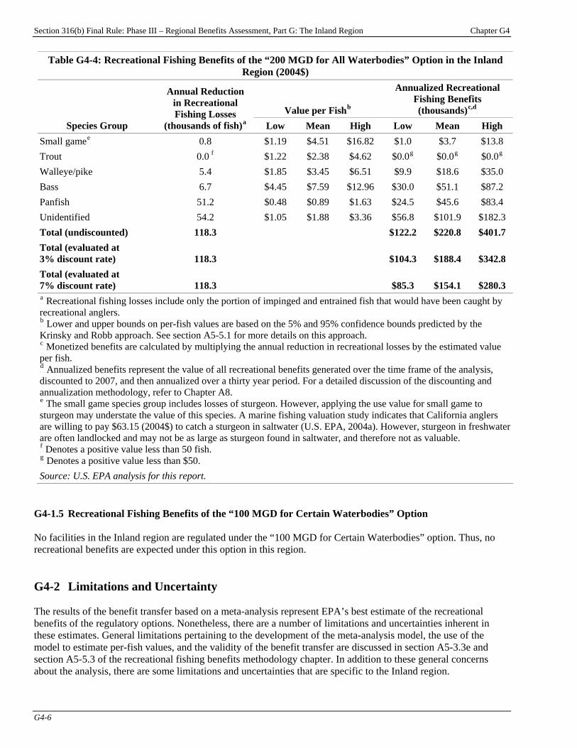
Section 316(b) Final Rule: Phase III – Regional Benefits Assessment, Part G: The Inland Region Chapter G4
G4-6
Table G4-4: Recreational Fishing Benefits of the “200 MGD for All Waterbodies” Option in the Inland Region (2004$)
Value per FishP
bP
Annualized Recreational Fishing Benefits (thousands)P
c,dP
Species Group
Annual Reduction in Recreational Fishing Losses
(thousands of fish)P
aP Low Mean High Low Mean High
Small gameP
eP 0.8 $1.19 $4.51 $16.82 $1.0 $3.7 $13.8
Trout 0.0P
fP $1.22 $2.38 $4.62 $0.0P
gP $0.0P
gP $0.0P
gP
Walleye/pike 5.4 $1.85 $3.45 $6.51 $9.9 $18.6 $35.0 Bass 6.7 $4.45 $7.59 $12.96 $30.0 $51.1 $87.2 Panfish 51.2 $0.48 $0.89 $1.63 $24.5 $45.6 $83.4 Unidentified 54.2 $1.05 $1.88 $3.36 $56.8 $101.9 $182.3 Total (undiscounted) 118.3 $122.2 $220.8 $401.7 Total (evaluated at 3% discount rate) 118.3 $104.3 $188.4 $342.8 Total (evaluated at 7% discount rate) 118.3 $85.3 $154.1 $280.3 P
aP Recreational fishing losses include only the portion of impinged and entrained fish that would have been caught by
recreational anglers. P
bP Lower and upper bounds on per-fish values are based on the 5% and 95% confidence bounds predicted by the
Krinsky and Robb approach. See section A5-5.1 for more details on this approach. P
cP Monetized benefits are calculated by multiplying the annual reduction in recreational losses by the estimated value
per fish. P
dP Annualized benefits represent the value of all recreational benefits generated over the time frame of the analysis,
discounted to 2007, and then annualized over a thirty year period. For a detailed discussion of the discounting and annualization methodology, refer to Chapter A8. P
eP The small game species group includes losses of sturgeon. However, applying the use value for small game to
sturgeon may understate the value of this species. A marine fishing valuation study indicates that California anglers are willing to pay $63.15 (2004$) to catch a sturgeon in saltwater (U.S. EPA, 2004a). However, sturgeon in freshwater are often landlocked and may not be as large as sturgeon found in saltwater, and therefore not as valuable. P
fP Denotes a positive value less than 50 fish.
P
gP Denotes a positive value less than $50.
Source: U.S. EPA analysis for this report. G4-1.5 Recreational Fishing Benefits of the “100 MGD for Certain Waterbodies” Option No facilities in the Inland region are regulated under the “100 MGD for Certain Waterbodies” option. Thus, no recreational benefits are expected under this option in this region. G4-2 Limitations and Uncertainty The results of the benefit transfer based on a meta-analysis represent EPA’s best estimate of the recreational benefits of the regulatory options. Nonetheless, there are a number of limitations and uncertainties inherent in these estimates. General limitations pertaining to the development of the meta-analysis model, the use of the model to estimate per-fish values, and the validity of the benefit transfer are discussed in section A5-3.3e and section A5-5.3 of the recreational fishing benefits methodology chapter. In addition to these general concerns about the analysis, there are some limitations and uncertainties that are specific to the Inland region.

Section 316(b) Final Rule: Phase III – Regional Benefits Assessment, Part G: The Inland Region Chapter G4
G4-7
One limitation of applying the meta-analysis to the Inland region is that the Inland region is extremely diverse (by definition, it includes the entire continental U.S.). The studies used for the meta-analysis were conducted in only a few geographic regions. In particular, most of the studies that evaluated WTP for walleye, pike, and panfish were conducted in the Great Lakes (in Michigan or Wisconsin). Thus, the average values per fish predicted by the regression equation may not represent the actual value per fish in all areas of the U.S. Another limitation of the analysis is that EPA was unable to locate any studies that evaluated WTP for channel catfish or for freshwater drum, two species with high I&E losses in the Inland region. However, the Agency believes that the per-fish values for channel catfish and freshwater drum can be approximated by the per-fish values for “panfish” and “unidentified” species, respectively.
Section 316(b) Final Rule: Phase III – Regional Benefits Assessment, Part G: The Inland Region Appendix G4
App. G4-1
Appendix G4: Recreational Use Benefits Under Supplemental Policy Options
Introduction
Appendix Contents G4-1 Recreational Fishing Benefits of the Supplemental Options ...................................G4-1 G4-1.1 Estimated Reductions in Recreational Fishing Losses Under the Supplemental Options.....G4-1 G4-1.2 Recreational Fishing Benefits of the Supplemental Options ...........G4-4G4-2 Comparison of Recreational Fishing Benefits by Option ......................................G4-12
Chapter G4 presents EPA’s estimates of the recreational benefits of the three regulatory options for the section 316(b) rule for Phase III facilities in the Inland region. To facilitate comparisons among the options, this appendix presents estimates of the recreational fishing benefits of various supplemental options that EPA evaluated in preparation for this rule:
< “Electric Generators 2-50 MGD I-only Everywhere” option;
< “Electric Generators 2-50 MGD I&E like Phase II” option; < “Electric Generators 2-50 MGD I&E Everywhere” option; < “Manufacturers 2-50 MGD I-only Everywhere” option; < “Manufacturers 2-50 MGD I&E like Phase II” option; < “Manufacturers 2-50 MGD I&E Everywhere” option; < “Manufacturers 50+ MGD I-only Everywhere” option; and < “Manufacturers 50+ MGD I&E Everywhere” option.
For additional information on the options, please see the TDD. Recreational fishing benefits presented in this chapter were estimated using the benefit transfer approach discussed in Chapter G4 and in Chapter A5, “Recreational Fishing Benefits Methodology.” G4-1 Recreational Fishing Benefits of the Supplemental Options G4-1.1 Estimated Reductions in Recreational Fishing Losses Under the Supplemental Options Table G4-1 presents EPA’s estimates of the annual reduction in baseline (i.e., current) recreational fishing losses from impingement and entrainment (I&E) in the Inland region under the supplemental options.

Section 316(b) Final Rule: Phase III – Regional Benefits Assessment, Part G: The Inland Region Appendix G4
App. G4-2
Table G4-1: Reductions in Recreational Fishing Losses from I&E Under the Supplemental Options in the Inland Region Annual Reduction in Recreational Losses
(# of fish) Electric Generators 2-50 MGD Manufacturers 2-50 MGD Manufacturers 50+ MGD
SpeciesP
a,bP
I-only Everywhere
I&E like Phase II
I&E Everywhere
I-only Everywhere
I&E like Phase II
I&E Everywhere
I-only Everywhere
I&E Everywhere
American shad 4.7 4.7 4.7 32.8 32.8 32.8 160.1 160.1 PaddlefishP
cP 3.0 3.3 5.2 21.2 23.5 31.5 103.8 158.9
Striped bass 29.8 29.8 29.8 208.9 208.9 208.9 1,021.0 1,021.0 SturgeonP
cP 0.3 0.6 2.7 2.3 4.8 13.6 11.4 72.3
Total (small game) 37.8 38.3 42.4 265.2 270.0 286.8 1,296.2 1,412.3 Northern pike 0.0 0.0 0.0 0.3 0.3 0.3 1.4 1.4 Sauger 14.2 43.8 282.2 99.6 381.1 1,374.7 486.6 7,359.9 Walleye 0.5 32.4 288.4 3.8 306.3 1,373.7 18.7 7,402.3
Total (walleye/pike) 14.8 76.2 570.6 103.7 687.7 2,748.7 506.7 14,763.6 Smallmouth bass 16.9 37.4 202.8 118.5 313.8 1,003.0 579.0 5,346.7 Spotted bass 0.1 0.1 0.1 0.9 0.9 0.9 4.3 4.3 White bass 196.4 204.3 267.8 1,377.1 1,452.1 1,716.9 6,729.8 8,561.0
Total (bass) 213.4 241.9 470.7 1,496.5 1,766.8 2,720.7 7,313.1 13,912.0 Black bullhead 2.1 2.1 2.1 14.6 14.6 14.6 71.3 71.3 Black crappie 5.7 5.7 5.7 40.0 40.0 40.1 195.3 196.2 Bluegill 606.6 611.9 654.8 4,252.7 4,303.4 4,482.3 20,782.2 22,019.8 Brown bullhead 17.8 21.5 51.3 124.7 159.9 284.2 609.5 1,468.9 Bullhead 17.3 20.4 45.0 121.5 150.6 253.3 593.5 1,304.4 Channel catfish 411.4 430.8 587.1 2,884.4 3,069.1 3,720.7 14,095.6 18,603.3 Crappie 43.4 97.2 529.9 304.6 815.7 2,619.7 1,488.4 13,967.4 Menhaden 0.5 0.5 0.5 3.3 3.3 3.3 16.1 16.1 Sunfish 349.7 464.1 1,384.2 2,452.0 3,538.9 7,374.8 11,982.5 38,517.2 White perch 1.9 2.0 2.9 13.5 14.5 18.1 66.1 91.0 Yellow perch 223.4 226.1 247.6 1,566.6 1,592.0 1,681.5 7,655.6 8,275.1

316(b) Final Rule: Phase III – Regional Benefits Assessment, Part G: The Inland Region Appendix G4
App. G4-3
0.1 0.1 0.1 0.6 0.6 0.6 3.0 3.1 0.1 0.1 0.1 0.6 0.6 0.6 3.0 3.1
1,694.8 1,930.1 3,823.5 11,882.4 14,118.9 22,012.5 58,066.8 112,669.6
1,679.9 1,882.3 3,511.2 11,777.9 13,702.0 20,492.8 57,556.3 104,530.7
3,640.9 4,168.9 8,418.5 25,526.3 30,546.0 48,262.2 124,742.1 247,291.1
Table G4-1: Reductions in Recreational Fishing Losses from I&E Under the Supplemental Options in the Inland Region Annual Reduction in Recreational Losses
(# of fish) Electric Generators 2-50 MGD Manufacturers 2-50 MGD Manufacturers 50+ MGD
SpeciesP
a,bP
I-only Everywhere
I&E like Phase II
I&E Everywhere
I-only Everywhere
I&E like Phase II
I&E Everywhere
I-only Everywhere
I&E Everywhere
Total (panfish)
P
aP EPA assigned each species with I&E losses to one of the species groups used in the meta-analysis. The “unidentified” group includes fish lost indirectly through
trophic transfer, fish reported lost without information about their species, and freshwater drum. Freshwater drum were included in this group because there were no valuation studies available and this species does not correspond well with any of the other species groups P
bP This table includes several species of anadromous fish (such as American shad and striped bass) that are classified in saltwater species groups, but that are
commonly caught in freshwater during part of their life cycle. P
cP No valuation studies were available for freshwater sturgeon or paddlefish. EPA included these two species in the “small game” group because the typical size of
these species is consistent with (or larger than) the size of other species in the “small game” group. Adult lake sturgeon generally weigh 10 to 80 pounds and measure three to five feet in length, and may grow as large as 300 pounds and seven feet long (NYSDEC, 2003). White sturgeon, which are anadromous, can grow to 400 pounds or 10 feet in length (Monterey Bay Aquarium, 1999). Paddlefish are also very large, averaging between 3.3 and 4.8 feet in length (Jenkins and Burkhead, 1993). P
dP EPA included whitefish in the “trout” category because its physical characteristics are similar to trout, and lake whitefish are prized for their meat. Therefore,
valuing them in the panfish category would be inappropriate. Source: U.S. EPA analysis for this report.
Total (unidentified) Total (all species)
WhitefishP
dP
Total (trout)
Section
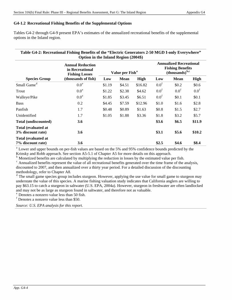
Section 316(b) Final Rule: Phase III – Regional Benefits Assessment, Part G: The Inland Region Appendix G4
App. G4-4
G4-1.2 Recreational Fishing Benefits of the Supplemental Options Tables G4-2 through G4-9 present EPA’s estimates of the annualized recreational benefits of the supplemental options in the Inland region.
Table G4-2: Recreational Fishing Benefits of the “Electric Generators 2-50 MGD I-only Everywhere” Option in the Inland Region (2004$)
Value per FishP
aP
Annualized Recreational Fishing Benefits (thousands)P
b,cP
Species Group
Annual Reduction in Recreational Fishing Losses
(thousands of fish) Low Mean High Low Mean High Small GameP
dP 0.0P
eP $1.19 $4.51 $16.82 0.0P
fP $0.2 $0.6
Trout 0.0P
eP $1.22 $2.38 $4.62 0.0P
fP 0.0P
fP 0.0P
fP
Walleye/Pike 0.0P
eP $1.85 $3.45 $6.51 0.0P
fP $0.1 $0.1
Bass 0.2 $4.45 $7.59 $12.96 $1.0 $1.6 $2.8 Panfish 1.7 $0.48 $0.89 $1.63 $0.8 $1.5 $2.7 Unidentified 1.7 $1.05 $1.88 $3.36 $1.8 $3.2 $5.7 Total (undiscounted) 3.6 $3.6 $6.5 $11.9 Total (evaluated at 3% discount rate) 3.6 $3.1 $5.6 $10.2 Total (evaluated at 7% discount rate) 3.6 $2.5 $4.6 $8.4 P
aP Lower and upper bounds on per-fish values are based on the 5% and 95% confidence bounds predicted by the
Krinsky and Robb approach. See section A5-5.1 of Chapter A5 for more details on this approach. P
bP Monetized benefits are calculated by multiplying the reduction in losses by the estimated value per fish.
P
cP Annualized benefits represent the value of all recreational benefits generated over the time frame of the analysis,
discounted to 2007, and then annualized over a thirty year period. For a detailed discussion of the discounting methodology, refer to Chapter A8. P
dP The small game species group includes sturgeon. However, applying the use value for small game to sturgeon may
understate the value of this species. A marine fishing valuation study indicates that California anglers are willing to pay $63.15 to catch a sturgeon in saltwater (U.S. EPA, 2004a). However, sturgeon in freshwater are often landlocked and may not be as large as sturgeon found in saltwater, and therefore not as valuable. P
eP Denotes a nonzero value less than 50 fish.
P
fP Denotes a nonzero value less than $50.
Source: U.S. EPA analysis for this report.

Section 316(b) Final Rule: Phase III – Regional Benefits Assessment, Part G: The Inland Region Appendix G4
App. G4-5
Table G4-3: Recreational Fishing Benefits of the “Electric Generators 2-50 MGD I&E like Phase II” Option in the Inland Region (2004$)
Value per FishP
aP
Annualized Recreational Fishing Benefits (thousands)P
b,cP
Species Group
Annual Reduction in Recreational Fishing Losses
(thousands of fish) Low Mean High Low Mean High Small GameP
dP 0.0P
eP $1.19 $4.51 $16.82 0.0P
fP $0.2 $0.6
Trout 0.0P
eP $1.22 $2.38 $4.62 0.0P
fP 0.0P
fP 0.0P
fP
Walleye/Pike 0.1 $1.85 $3.45 $6.51 $0.1 $0.3 $0.5 Bass 0.2 $4.45 $7.59 $12.96 $1.1 $1.8 $3.1 Panfish 1.9 $0.48 $0.89 $1.63 $0.9 $1.7 $3.1 Unidentified 1.9 $1.05 $1.88 $3.36 $2.0 $3.6 $6.5 Total (undiscounted) 4.2 $4.2 $7.6 $13.8 Total (evaluated at 3% discount rate) 4.2 $3.6 $6.5 $11.9 Total (evaluated at 7% discount rate) 4.2 $3.0 $5.4 $9.8 P
aP Lower and upper bounds on per-fish values are based on the 5% and 95% confidence bounds predicted by the
Krinsky and Robb approach. See section A5-5.1 of Chapter A5 for more details on this approach. P
bP Monetized benefits are calculated by multiplying the reduction in losses by the estimated value per fish.
P
cP Annualized benefits represent the value of all recreational benefits generated over the time frame of the analysis,
discounted to 2007, and then annualized over a thirty year period. For a detailed discussion of the discounting methodology, refer to Chapter A8. P
dP The small game species group includes sturgeon. However, applying the use value for small game to sturgeon may
understate the value of this species. A marine fishing valuation study indicates that California anglers are willing to pay $61.43 to catch a sturgeon in saltwater (U.S. EPA, 2004a). However, sturgeon in freshwater are often landlocked and may not be as large as sturgeon found in saltwater, and therefore not as valuable. P
eP Denotes a nonzero value less than 50 fish.
P
fP Denotes a nonzero value less than $50.
Source: U.S. EPA analysis for this report.
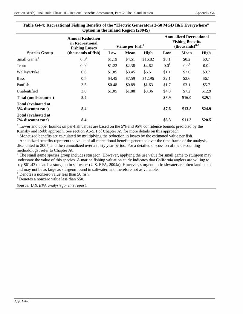
Section 316(b) Final Rule: Phase III – Regional Benefits Assessment, Part G: The Inland Region Appendix G4
App. G4-6
Table G4-4: Recreational Fishing Benefits of the “Electric Generators 2-50 MGD I&E Everywhere” Option in the Inland Region (2004$)
Value per FishP
aP
Annualized Recreational Fishing Benefits (thousands)P
b,cP
Species Group
Annual Reduction in Recreational Fishing Losses
(thousands of fish) Low Mean High Low Mean High Small GameP
dP 0.0P
eP $1.19 $4.51 $16.82 $0.1 $0.2 $0.7
Trout 0.0P
eP $1.22 $2.38 $4.62 0.0P
fP 0.0P
fP 0.0P
fP
Walleye/Pike 0.6 $1.85 $3.45 $6.51 $1.1 $2.0 $3.7 Bass 0.5 $4.45 $7.59 $12.96 $2.1 $3.6 $6.1 Panfish 3.5 $0.48 $0.89 $1.63 $1.7 $3.1 $5.7 Unidentified 3.8 $1.05 $1.88 $3.36 $4.0 $7.2 $12.9 Total (undiscounted) 8.4 $8.9 $16.0 $29.1 Total (evaluated at 3% discount rate) 8.4 $7.6 $13.8 $24.9 Total (evaluated at 7% discount rate) 8.4 $6.3 $11.3 $20.5 P
aP Lower and upper bounds on per-fish values are based on the 5% and 95% confidence bounds predicted by the
Krinsky and Robb approach. See section A5-5.1 of Chapter A5 for more details on this approach. P
bP Monetized benefits are calculated by multiplying the reduction in losses by the estimated value per fish.
P
cP Annualized benefits represent the value of all recreational benefits generated over the time frame of the analysis,
discounted to 2007, and then annualized over a thirty year period. For a detailed discussion of the discounting methodology, refer to Chapter A8. P
dP The small game species group includes sturgeon. However, applying the use value for small game to sturgeon may
understate the value of this species. A marine fishing valuation study indicates that California anglers are willing to pay $61.43 to catch a sturgeon in saltwater (U.S. EPA, 2004a). However, sturgeon in freshwater are often landlocked and may not be as large as sturgeon found in saltwater, and therefore not as valuable. P
eP Denotes a nonzero value less than 50 fish.
P
fP Denotes a nonzero value less than $50.
Source: U.S. EPA analysis for this report.
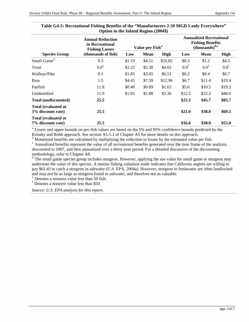
Section 316(b) Final Rule: Phase III – Regional Benefits Assessment, Part G: The Inland Region Appendix G4
App. G4-7
Table G4-5: Recreational Fishing Benefits of the “Manufacturers 2-50 MGD I-only Everywhere” Option in the Inland Region (2004$)
Value per FishP
aP
Annualized Recreational Fishing Benefits (thousands)P
b,cP
Species Group
Annual Reduction in Recreational Fishing Losses
(thousands of fish) Low Mean High Low Mean High Small GameP
dP 0.3 $1.19 $4.51 $16.82 $0.3 $1.2 $4.5
Trout 0.0P
eP $1.22 $2.38 $4.62 0.0P
fP 0.0P
fP 0.0P
fP
Walleye/Pike 0.1 $1.85 $3.45 $6.51 $0.2 $0.4 $0.7 Bass 1.5 $4.45 $7.59 $12.96 $6.7 $11.4 $19.4 Panfish 11.8 $0.48 $0.89 $1.63 $5.6 $10.5 $19.2 Unidentified 11.9 $1.05 $1.88 $3.36 $12.5 $22.3 $40.0 Total (undiscounted) 25.5 $25.3 $45.7 $83.7 Total (evaluated at 3% discount rate) 25.5 $21.0 $38.0 $69.5 Total (evaluated at 7% discount rate) 25.5 $16.6 $30.0 $55.0 P
aP Lower and upper bounds on per-fish values are based on the 5% and 95% confidence bounds predicted by the
Krinsky and Robb approach. See section A5-5.1 of Chapter A5 for more details on this approach. P
bP Monetized benefits are calculated by multiplying the reduction in losses by the estimated value per fish.
P
cP Annualized benefits represent the value of all recreational benefits generated over the time frame of the analysis,
discounted to 2007, and then annualized over a thirty year period. For a detailed discussion of the discounting methodology, refer to Chapter A8. P
dP The small game species group includes sturgeon. However, applying the use value for small game to sturgeon may
understate the value of this species. A marine fishing valuation study indicates that California anglers are willing to pay $61.43 to catch a sturgeon in saltwater (U.S. EPA, 2004a). However, sturgeon in freshwater are often landlocked and may not be as large as sturgeon found in saltwater, and therefore not as valuable. P
eP Denotes a nonzero value less than 50 fish.
P
fP Denotes a nonzero value less than $50.
Source: U.S. EPA analysis for this report.

Section 316(b) Final Rule: Phase III – Regional Benefits Assessment, Part G: The Inland Region Appendix G4
App. G4-8
Table G4-6: Recreational Fishing Benefits of the “Manufacturers 2-50 MGD I&E like Phase II” Option in the Inland Region (2004$)
Value per FishP
aP
Annualized Recreational Fishing Benefits (thousands)P
b,cP
Species Group
Annual Reduction in Recreational Fishing Losses
(thousands of fish) Low Mean High Low Mean High Small GameP
dP 0.3 $1.19 $4.51 $16.82 $0.3 $1.2 $4.5
Trout 0.0P
eP $1.22 $2.38 $4.62 0.0P
fP 0.0P
fP 0.0P
fP
Walleye/Pike 0.7 $1.85 $3.45 $6.51 $1.3 $2.4 $4.5 Bass 1.8 $4.45 $7.59 $12.96 $7.9 $13.4 $22.9 Panfish 13.7 $0.48 $0.89 $1.63 $6.6 $12.2 $22.3 Unidentified 14.1 $1.05 $1.88 $3.36 $14.8 $26.5 $47.5 Total (undiscounted) 30.5 $30.8 $55.7 $101.7 Total (evaluated at 3% discount rate) 30.5 $25.7 $46.4 $84.7 Total (evaluated at 7% discount rate) 30.5 $20.4 $36.8 $67.2 P
aP Lower and upper bounds on per-fish values are based on the 5% and 95% confidence bounds predicted by the
Krinsky and Robb approach. See section A5-5.1 of Chapter A5 for more details on this approach. P
bP Monetized benefits are calculated by multiplying the reduction in losses by the estimated value per fish.
P
cP Annualized benefits represent the value of all recreational benefits generated over the time frame of the analysis,
discounted to 2007, and then annualized over a thirty year period. For a detailed discussion of the discounting methodology, refer to Chapter A8. P
dP The small game species group includes sturgeon. However, applying the use value for small game to sturgeon may
understate the value of this species. A marine fishing valuation study indicates that California anglers are willing to pay $61.43 to catch a sturgeon in saltwater (U.S. EPA, 2004a). However, sturgeon in freshwater are often landlocked and may not be as large as sturgeon found in saltwater, and therefore not as valuable. P
eP Denotes a nonzero value less than 50 fish.
P
fP Denotes a nonzero value less than $50.
Source: U.S. EPA analysis for this report.
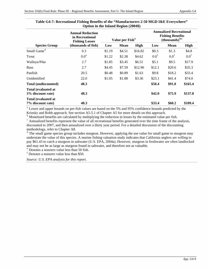
Section 316(b) Final Rule: Phase III – Regional Benefits Assessment, Part G: The Inland Region Appendix G4
App. G4-9
Table G4-7: Recreational Fishing Benefits of the “Manufacturers 2-50 MGD I&E Everywhere” Option in the Inland Region (2004$)
Value per FishP
aP
Annualized Recreational Fishing Benefits (thousands)P
b,cP
Species Group
Annual Reduction in Recreational Fishing Losses
(thousands of fish) Low Mean High Low Mean High Small GameP
dP 0.3 $1.19 $4.51 $16.82 $0.3 $1.3 $4.8
Trout 0.0P
eP $1.22 $2.38 $4.62 0.0P
fP 0.0P
fP 0.0P
fP
Walleye/Pike 2.7 $1.85 $3.45 $6.51 $5.1 $9.5 $17.9 Bass 2.7 $4.45 $7.59 $12.96 $12.1 $20.6 $35.3 Panfish 20.5 $0.48 $0.89 $1.63 $9.8 $18.2 $33.4 Unidentified 22.0 $1.05 $1.88 $3.36 $23.1 $41.4 $74.0 Total (undiscounted) 48.3 $50.4 $91.0 $165.4 Total (evaluated at 3% discount rate) 48.3 $42.0 $75.9 $137.8 Total (evaluated at 7% discount rate) 48.3 $33.4 $60.2 $109.4 P
aP Lower and upper bounds on per-fish values are based on the 5% and 95% confidence bounds predicted by the
Krinsky and Robb approach. See section A5-5.1 of Chapter A5 for more details on this approach. P
bP Monetized benefits are calculated by multiplying the reduction in losses by the estimated value per fish.
P
cP Annualized benefits represent the value of all recreational benefits generated over the time frame of the analysis,
discounted to 2007, and then annualized over a thirty year period. For a detailed discussion of the discounting methodology, refer to Chapter A8. P
dP The small game species group includes sturgeon. However, applying the use value for small game to sturgeon may
understate the value of this species. A marine fishing valuation study indicates that California anglers are willing to pay $61.43 to catch a sturgeon in saltwater (U.S. EPA, 2004a). However, sturgeon in freshwater are often landlocked and may not be as large as sturgeon found in saltwater, and therefore not as valuable. P
eP Denotes a nonzero value less than 50 fish.
P
fP Denotes a nonzero value less than $50.
Source: U.S. EPA analysis for this report.

Section 316(b) Final Rule: Phase III – Regional Benefits Assessment, Part G: The Inland Region Appendix G4
App. G4-10
Table G4-8: Recreational Fishing Benefits of the “Manufacturers 50+ MGD I-only Everywhere” Option in the Inland Region (2004$)
Value per FishP
aP
Annualized Recreational Fishing Benefits (thousands)P
b,cP
Species Group
Annual Reduction in Recreational Fishing Losses
(thousands of fish) Low Mean High Low Mean High Small GameP
dP 1.3 $1.19 $4.51 $16.82 $1.5 $5.8 $21.8
Trout 0.0P
eP $1.22 $2.38 $4.62 0.0P
fP 0.0P
fP 0.0P
fP
Walleye/Pike 0.5 $1.85 $3.45 $6.51 $0.9 $1.8 $3.3 Bass 7.3 $4.45 $7.59 $12.96 $32.6 $55.5 $94.8 Panfish 57.6 $0.48 $0.89 $1.63 $27.6 $51.2 $93.8 Unidentified 58.1 $1.05 $1.88 $3.36 $60.9 $109.1 $195.2 Total (undiscounted) 124.7 $123.5 $223.4 $408.9 Total (evaluated at 3% discount rate) 124.7 $105.2 $190.4 $348.4 Total (evaluated at 7% discount rate) 124.7 $85.9 $155.4 $284.3 P
aP Lower and upper bounds on per-fish values are based on the 5% and 95% confidence bounds predicted by the
Krinsky and Robb approach. See section A5-5.1 of Chapter A5 for more details on this approach. P
bP Monetized benefits are calculated by multiplying the reduction in losses by the estimated value per fish.
P
cP Annualized benefits represent the value of all recreational benefits generated over the time frame of the analysis,
discounted to 2007, and then annualized over a thirty year period. For a detailed discussion of the discounting methodology, refer to Chapter A8. P
dP The small game species group includes sturgeon. However, applying the use value for small game to sturgeon may
understate the value of this species. A marine fishing valuation study indicates that California anglers are willing to pay $61.43 to catch a sturgeon in saltwater (U.S. EPA, 2004a). However, sturgeon in freshwater are often landlocked and may not be as large as sturgeon found in saltwater, and therefore not as valuable. P
eP Denotes a nonzero value less than 50 fish.
P
fP Denotes a nonzero value less than $50.
Source: U.S. EPA analysis for this report.
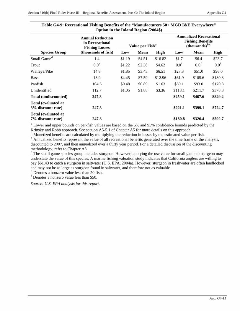
Section 316(b) Final Rule: Phase III – Regional Benefits Assessment, Part G: The Inland Region Appendix G4
App. G4-11
Table G4-9: Recreational Fishing Benefits of the “Manufacturers 50+ MGD I&E Everywhere” Option in the Inland Region (2004$)
Value per FishP
aP
Annualized Recreational Fishing Benefits (thousands)P
b,cP
Species Group
Annual Reduction in Recreational Fishing Losses
(thousands of fish) Low Mean High Low Mean High Small GameP
dP 1.4 $1.19 $4.51 $16.82 $1.7 $6.4 $23.7
Trout 0.0P
eP $1.22 $2.38 $4.62 0.0P
fP 0.0P
fP 0.0P
fP
Walleye/Pike 14.8 $1.85 $3.45 $6.51 $27.3 $51.0 $96.0 Bass 13.9 $4.45 $7.59 $12.96 $61.9 $105.6 $180.3 Panfish 104.5 $0.48 $0.89 $1.63 $50.1 $93.0 $170.3 Unidentified 112.7 $1.05 $1.88 $3.36 $118.1 $211.7 $378.8 Total (undiscounted) 247.3 $259.1 $467.6 $849.2 Total (evaluated at 3% discount rate) 247.3 $221.1 $399.1 $724.7 Total (evaluated at 7% discount rate) 247.3 $180.8 $326.4 $592.7 P
aP Lower and upper bounds on per-fish values are based on the 5% and 95% confidence bounds predicted by the
Krinsky and Robb approach. See section A5-5.1 of Chapter A5 for more details on this approach. P
bP Monetized benefits are calculated by multiplying the reduction in losses by the estimated value per fish.
P
cP Annualized benefits represent the value of all recreational benefits generated over the time frame of the analysis,
discounted to 2007, and then annualized over a thirty year period. For a detailed discussion of the discounting methodology, refer to Chapter A8. P
dP The small game species group includes sturgeon. However, applying the use value for small game to sturgeon may
understate the value of this species. A marine fishing valuation study indicates that California anglers are willing to pay $61.43 to catch a sturgeon in saltwater (U.S. EPA, 2004a). However, sturgeon in freshwater are often landlocked and may not be as large as sturgeon found in saltwater, and therefore not as valuable. P
eP Denotes a nonzero value less than 50 fish.
P
fP Denotes a nonzero value less than $50.
Source: U.S. EPA analysis for this report.

Section 316(b) Final Rule: Phase III – Regional Benefits Assessment, Part G: The Inland Region Appendix G4
App. G4-12
G4-2 Comparison of Recreational Fishing Benefits by Option Table G4-10 compares the recreational fishing benefits of some supplemental options.
Table G4-10: Annual Recreational Benefits of the Supplemental Options in the Inland Region Undiscounted Recreational Fishing Benefits
(thousands; 2004$)P
aP
Policy Option
Annual Reduction in Recreational Fishing
Losses from I&E (thousands of fish) Low Mean High
Electric Generators 2-50 MGD I-only Everywhere 3.6 $3.6 $6.5 $11.9 I&E like Phase II 4.2 $4.2 $7.6 $13.8 I&E Everywhere 8.4 $8.9 $16.0 $29.1
Manufacturers 2-50 MGD I-only Everywhere 25.5 $25.3 $45.7 $83.7 I&E like Phase II 30.5 $30.8 $55.7 $101.7 I&E Everywhere 48.3 $50.4 $91.0 $165.4
Manufacturers 50+ MGD I-only Everywhere 124.7 $123.5 $223.4 $408.9 I&E Everywhere 247.3 $259.1 $467.6 $849.2
P
aP These benefit estimates were calculated using the meta-analysis approach discussed in Chapter A5 and Chapter B4.
Source: U.S. EPA analysis for this report.
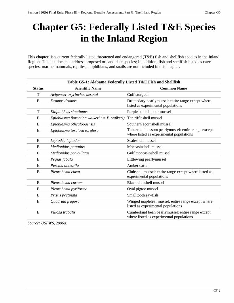
Section 316(b) Final Rule: Phase III – Regional Benefits Assessment, Part G: The Inland Region Chapter G5
G5-1
Chapter G5: Federally Listed T&E Species in the Inland Region
This chapter lists current federally listed threatened and endangered (T&E) fish and shellfish species in the Inland Region. This list does not address proposed or candidate species; In addition, fish and shellfish listed as cave species, marine mammals, reptiles, amphibians, and snails are not included in this chapter.
Table G5-1: Alabama Federally Listed T&E Fish and Shellfish Status Scientific Name Common Name
T Acipenser oxyrinchus desotoi Gulf sturgeon E Dromus dromas Dromedary pearlymussel: entire range except where
listed as experimental populations T Elliptoideus sloatianus Purple bankclimber mussel E Epioblasma florentina walkeri ( = E. walkeri) Tan riffleshell mussel E Epioblasma othcaloogensis Southern acornshell mussel E Epioblasma torulosa torulosa Tubercled blossom pearlymussel: entire range except
where listed as experimental populations E Leptodea leptodon Scaleshell mussel E Medionidus parvulus Moccasinshell mussel E Medionidus penicillatus Gulf moccasinshell mussel E Pegias fabula Littlewing pearlymussel E Percina antesella Amber darter E Pleurobema clava Clubshell mussel: entire range except where listed as
experimental populations E Pleurobema curtum Black clubshell mussel E Pleurobema pyriforme Oval pigtoe mussel E Pristis pectinata Smalltooth sawfish E Quadrula fragosa Winged mapleleaf mussel: entire range except where
listed as experimental populations E Villosa trabalis Cumberland bean pearlymussel: entire range except
where listed as experimental populations Source: USFWS, 2006a.
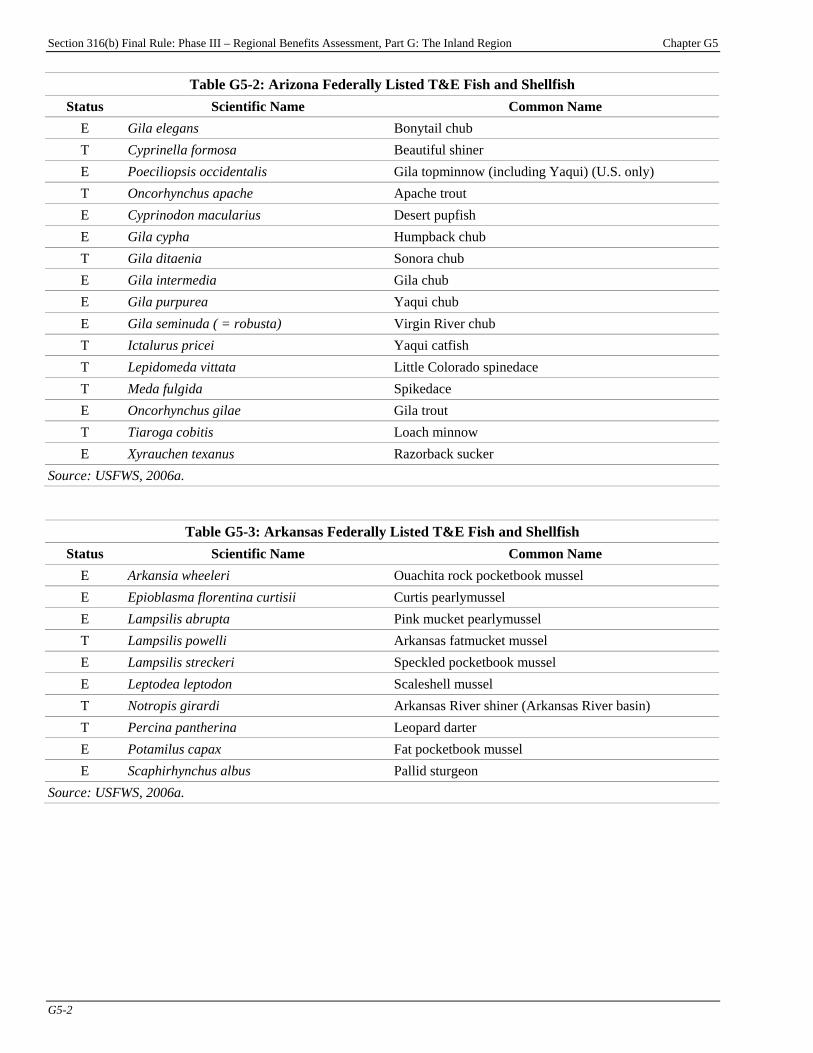
Section 316(b) Final Rule: Phase III – Regional Benefits Assessment, Part G: The Inland Region Chapter G5
G5-2
Table G5-2: Arizona Federally Listed T&E Fish and Shellfish Status Scientific Name Common Name
E Gila elegans Bonytail chub T Cyprinella formosa Beautiful shiner E Poeciliopsis occidentalis Gila topminnow (including Yaqui) (U.S. only) T Oncorhynchus apache Apache trout E Cyprinodon macularius Desert pupfish E Gila cypha Humpback chub T Gila ditaenia Sonora chub E Gila intermedia Gila chub E Gila purpurea Yaqui chub E Gila seminuda ( = robusta) Virgin River chub T Ictalurus pricei Yaqui catfish T Lepidomeda vittata Little Colorado spinedace T Meda fulgida Spikedace E Oncorhynchus gilae Gila trout T Tiaroga cobitis Loach minnow E Xyrauchen texanus Razorback sucker
Source: USFWS, 2006a.
Table G5-3: Arkansas Federally Listed T&E Fish and Shellfish Status Scientific Name Common Name
E Arkansia wheeleri Ouachita rock pocketbook mussel E Epioblasma florentina curtisii Curtis pearlymussel E Lampsilis abrupta Pink mucket pearlymussel T Lampsilis powelli Arkansas fatmucket mussel E Lampsilis streckeri Speckled pocketbook mussel E Leptodea leptodon Scaleshell mussel T Notropis girardi Arkansas River shiner (Arkansas River basin) T Percina pantherina Leopard darter E Potamilus capax Fat pocketbook mussel E Scaphirhynchus albus Pallid sturgeon
Source: USFWS, 2006a.

Section 316(b) Final Rule: Phase III – Regional Benefits Assessment, Part G: The Inland Region Chapter G5
G5-3
Table G5-4: California Federally Listed T&E Fish and Shellfish Status Scientific Name Common Name
E Branchinecta conservatio Conservancy fairy shrimp E Branchinecta longiantenna Longhorn fairy shrimp T Branchinecta lynchi Vernal pool fairy shrimp E Branchinecta sandiegonensis San Diego fairy shrimp E Catostomus microps Modoc sucker T Catostomus santaanae Santa Ana sucker (3 California river basins) E Chasmistes brevirostris Shortnose sucker E Cyprinodon macularius Desert pupfish E Cyprinodon radiosus Owens pupfish E Deltistes luxatus Lost River sucker E Eucyclogobius newberryi Tidewater goby E Gasterosteus aculeatus williamsoni Unarmored threespine stickleback E Gila bicolor mohavensis Mohave tui chub E Gila bicolor snyderi Owens tui chub E Gila elegans Bonytail chub T Haliotis sorenseni White abalone T Hypomesus transpacificus Delta smelt E Lepidurus packardi Vernal pool tadpole shrimp T Oncorhynchus ( = Salmo) kisutch Coho salmon (Oregon and California populations) E Oncorhynchus ( = Salmo) kisutch Coho salmon (central California coast) T Oncorhynchus ( = Salmo) mykiss Steelhead (Central Valley, California) T Oncorhynchus ( = Salmo) mykiss Steelhead (central California coast) T Oncorhynchus ( = Salmo) mykiss Steelhead (northern California) T Oncorhynchus ( = Salmo) mykiss Steelhead (south central California coast) E Oncorhynchus ( = Salmo) mykiss Steelhead (southern California coast) T Oncorhynchus ( = Salmo) tshawytscha Chinook salmon (California Central Valley) (spring run) T Oncorhynchus ( = Salmo) tshawytscha Chinook salmon (California coastal) E Oncorhynchus ( = Salmo) tshawytscha Chinook salmon (Sacramento River) (winter run) T Oncorhynchus aguabonita whitei Little Kern golden trout T Oncorhynchus clarki henshawi Lahontan cutthroat trout T Oncorhynchus clarki seleniris Paiute cutthroat trout E Pacifastacus fortis Shasta crayfish E Ptychocheilus lucius Pikeminnow ( = squawfish), Colorado except Salt and
Verde River drainages, AZ T Salvelinus confluentus Bull trout (U.S., conterminous, lower 48 states) E Streptocephalus woottoni Riverside fairy shrimp E Syncaris pacifica California freshwater shrimp E Xyrauchen texanus Razorback sucker
Source: USFWS, 2006a.

Section 316(b) Final Rule: Phase III – Regional Benefits Assessment, Part G: The Inland Region Chapter G5
G5-4
Table G5-5: Colorado Federally Listed T&E Fish and Shellfish Status Scientific Name Common Name
E Gila cypha Humpback chub E Gila elegans Bonytail chub E Ptychocheilus lucius Pikeminnow ( = squawfish), Colorado except Salt and
Verde R. drainages, AZ E Xyrauchen texanus Razorback sucker
Source: USFWS, 2006a.
Table G5-6: Connecticut Federally Listed T&E Fish and Shellfish Status Scientific Name Common Name
E Acipenser brevirostrum Shortnose sturgeon E Alasmidonta heterodon Dwarf wedgemussel
Source: USFWS, 2006a.
Table G5-7: Delaware Federally Listed T&E Fish and Shellfish Status Scientific Name Common Name
E Acipenser brevirostrum Shortnose sturgeon E Alasmidonta heterodon Dwarf wedgemussel
Source: USFWS, 2006a.
Table G5-8: District of Columbia Federally Listed T&E Fish and Shellfish Status Scientific Name Common Name
E Alasmidonta heterodon Dwarf wedgemussel Source: USFWS, 2006a.
Table G5-9: Florida Federally Listed T&E Fish and Shellfish Status Scientific Name Common Name
E Acipenser brevirostrum Shortnose sturgeon T Acipenser oxyrinchus desotoi Gulf sturgeon E Amblema neislerii Fat three-ridge mussel T Elliptio chipolaensis Chipola slabshell mussel T Elliptoideus sloatianus Purple bankclimber mussel E Etheostoma okaloosae Okaloosa darter E Lampsilis subangulata Shinyrayed pocketbook mussel E Medionidus penicillatus Gulf moccasinshell E Medionidus simpsonianus Ochlockonee moccasinshell E Pleurobema pyriforme Oval pigtoe mussel E Pristis pectinata Smalltooth sawfish
Source: USFWS, 2006a.
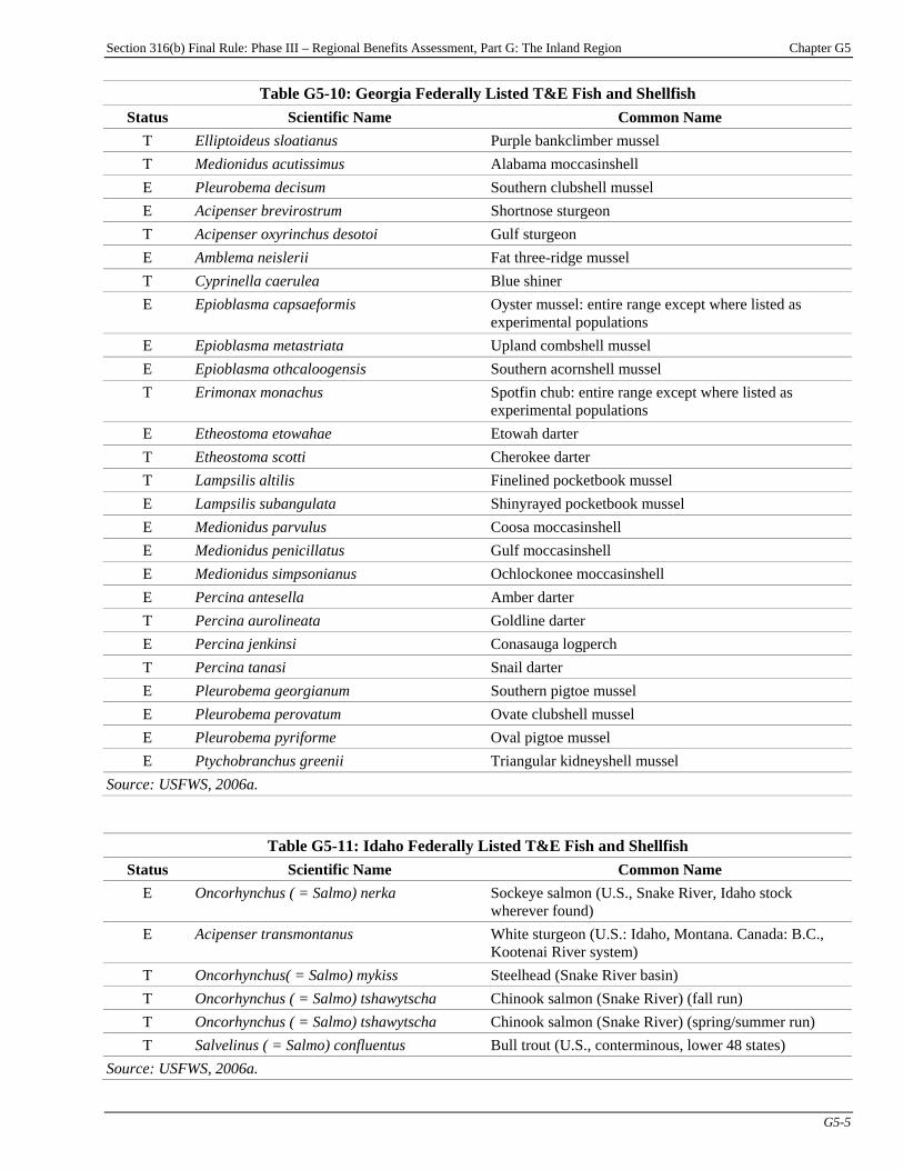
Section 316(b) Final Rule: Phase III – Regional Benefits Assessment, Part G: The Inland Region Chapter G5
G5-5
Table G5-10: Georgia Federally Listed T&E Fish and Shellfish Status Scientific Name Common Name
T Elliptoideus sloatianus Purple bankclimber mussel T Medionidus acutissimus Alabama moccasinshell E Pleurobema decisum Southern clubshell mussel E Acipenser brevirostrum Shortnose sturgeon T Acipenser oxyrinchus desotoi Gulf sturgeon E Amblema neislerii Fat three-ridge mussel T Cyprinella caerulea Blue shiner E Epioblasma capsaeformis Oyster mussel: entire range except where listed as
experimental populations E Epioblasma metastriata Upland combshell mussel E Epioblasma othcaloogensis Southern acornshell mussel T Erimonax monachus Spotfin chub: entire range except where listed as
experimental populations E Etheostoma etowahae Etowah darter T Etheostoma scotti Cherokee darter T Lampsilis altilis Finelined pocketbook mussel E Lampsilis subangulata Shinyrayed pocketbook mussel E Medionidus parvulus Coosa moccasinshell E Medionidus penicillatus Gulf moccasinshell E Medionidus simpsonianus Ochlockonee moccasinshell E Percina antesella Amber darter T Percina aurolineata Goldline darter E Percina jenkinsi Conasauga logperch T Percina tanasi Snail darter E Pleurobema georgianum Southern pigtoe mussel E Pleurobema perovatum Ovate clubshell mussel E Pleurobema pyriforme Oval pigtoe mussel E Ptychobranchus greenii Triangular kidneyshell mussel
Source: USFWS, 2006a.
Table G5-11: Idaho Federally Listed T&E Fish and Shellfish Status Scientific Name Common Name
E Oncorhynchus ( = Salmo) nerka Sockeye salmon (U.S., Snake River, Idaho stock wherever found)
E Acipenser transmontanus White sturgeon (U.S.: Idaho, Montana. Canada: B.C., Kootenai River system)
T Oncorhynchus( = Salmo) mykiss Steelhead (Snake River basin) T Oncorhynchus ( = Salmo) tshawytscha Chinook salmon (Snake River) (fall run) T Oncorhynchus ( = Salmo) tshawytscha Chinook salmon (Snake River) (spring/summer run) T Salvelinus ( = Salmo) confluentus Bull trout (U.S., conterminous, lower 48 states)
Source: USFWS, 2006a.
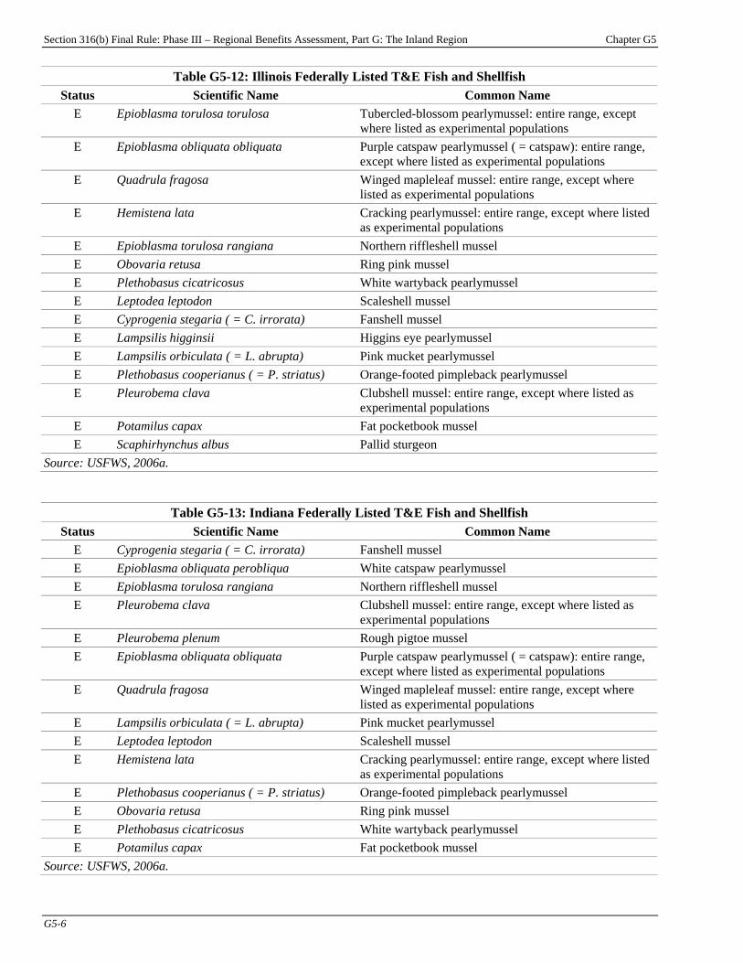
Section 316(b) Final Rule: Phase III – Regional Benefits Assessment, Part G: The Inland Region Chapter G5
G5-6
Table G5-12: Illinois Federally Listed T&E Fish and Shellfish Status Scientific Name Common Name
E Epioblasma torulosa torulosa Tubercled-blossom pearlymussel: entire range, except where listed as experimental populations
E Epioblasma obliquata obliquata Purple catspaw pearlymussel ( = catspaw): entire range, except where listed as experimental populations
E Quadrula fragosa Winged mapleleaf mussel: entire range, except where listed as experimental populations
E Hemistena lata Cracking pearlymussel: entire range, except where listed as experimental populations
E Epioblasma torulosa rangiana Northern riffleshell mussel E Obovaria retusa Ring pink mussel E Plethobasus cicatricosus White wartyback pearlymussel E Leptodea leptodon Scaleshell mussel E Cyprogenia stegaria ( = C. irrorata) Fanshell mussel E Lampsilis higginsii Higgins eye pearlymussel E Lampsilis orbiculata ( = L. abrupta) Pink mucket pearlymussel E Plethobasus cooperianus ( = P. striatus) Orange-footed pimpleback pearlymussel E Pleurobema clava Clubshell mussel: entire range, except where listed as
experimental populations E Potamilus capax Fat pocketbook mussel E Scaphirhynchus albus Pallid sturgeon
Source: USFWS, 2006a.
Table G5-13: Indiana Federally Listed T&E Fish and Shellfish Status Scientific Name Common Name
E Cyprogenia stegaria ( = C. irrorata) Fanshell mussel E Epioblasma obliquata perobliqua White catspaw pearlymussel E Epioblasma torulosa rangiana Northern riffleshell mussel E Pleurobema clava Clubshell mussel: entire range, except where listed as
experimental populations E Pleurobema plenum Rough pigtoe mussel E Epioblasma obliquata obliquata Purple catspaw pearlymussel ( = catspaw): entire range,
except where listed as experimental populations E Quadrula fragosa Winged mapleleaf mussel: entire range, except where
listed as experimental populations E Lampsilis orbiculata ( = L. abrupta) Pink mucket pearlymussel E Leptodea leptodon Scaleshell mussel E Hemistena lata Cracking pearlymussel: entire range, except where listed
as experimental populations E Plethobasus cooperianus ( = P. striatus) Orange-footed pimpleback pearlymussel E Obovaria retusa Ring pink mussel E Plethobasus cicatricosus White wartyback pearlymussel E Potamilus capax Fat pocketbook mussel
Source: USFWS, 2006a.
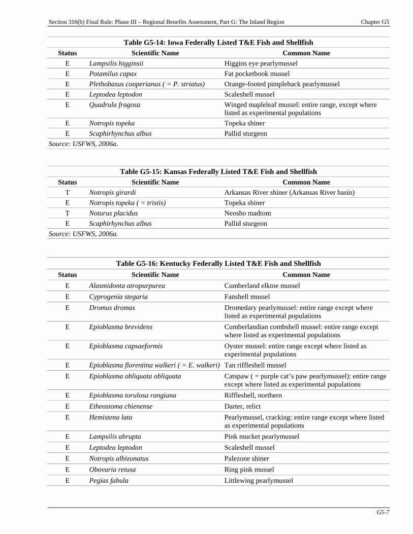
Section 316(b) Final Rule: Phase III – Regional Benefits Assessment, Part G: The Inland Region Chapter G5
G5-7
Table G5-14: Iowa Federally Listed T&E Fish and Shellfish Status Scientific Name Common Name
E Lampsilis higginsii Higgins eye pearlymussel E Potamilus capax Fat pocketbook mussel E Plethobasus cooperianus ( = P. striatus) Orange-footed pimpleback pearlymussel E Leptodea leptodon Scaleshell mussel E Quadrula fragosa Winged mapleleaf mussel: entire range, except where
listed as experimental populations E Notropis topeka Topeka shiner E Scaphirhynchus albus Pallid sturgeon
Source: USFWS, 2006a.
Table G5-15: Kansas Federally Listed T&E Fish and Shellfish Status Scientific Name Common Name
T Notropis girardi Arkansas River shiner (Arkansas River basin) E Notropis topeka ( = tristis) Topeka shiner T Noturus placidus Neosho madtom E Scaphirhynchus albus Pallid sturgeon
Source: USFWS, 2006a.
Table G5-16: Kentucky Federally Listed T&E Fish and Shellfish Status Scientific Name Common Name
E Alasmidonta atropurpurea Cumberland elktoe mussel E Cyprogenia stegaria Fanshell mussel E Dromus dromas Dromedary pearlymussel: entire range except where
listed as experimental populations E Epioblasma brevidens Cumberlandian combshell mussel: entire range except
where listed as experimental populations E Epioblasma capsaeformis Oyster mussel: entire range except where listed as
experimental populations E Epioblasma florentina walkeri ( = E. walkeri) Tan riffleshell mussel E Epioblasma obliquata obliquata Catspaw ( = purple cat’s paw pearlymussel): entire range
except where listed as experimental populations E Epioblasma torulosa rangiana Riffleshell, northern E Etheostoma chienense Darter, relict E Hemistena lata Pearlymussel, cracking: entire range except where listed
as experimental populations E Lampsilis abrupta Pink mucket pearlymussel E Leptodea leptodon Scaleshell mussel E Notropis albizonatus Palezone shiner E Obovaria retusa Ring pink mussel E Pegias fabula Littlewing pearlymussel

Section 316(b) Final Rule: Phase III – Regional Benefits Assessment, Part G: The Inland Region Chapter G5
G5-8
Table G5-16: Kentucky Federally Listed T&E Fish and Shellfish Status Scientific Name Common Name
T Phoxinus cumberlandensis Blackside dace E Plethobasus cicatricosus White wartyback pearlymussel E Plethobasus cooperianus Orangefoot pimpleback pearlymussel E Pleurobema clava Clubshell mussel: entire range except where listed as
experimental populations E Pleurobema plenum Rough pigtoe mussel E Potamilus capax Fat pocketbook mussel E Quadrula fragosa Winged mapleleaf mussel: entire range except where
listed as experimental populations E Scaphirhynchus albus Pallid sturgeon E Villosa trabalis Cumberland bean pearlymussel: entire range except
where listed as experimental populations Source: USFWS, 2006a.
Table G5-17: Louisiana Federally Listed T&E Fish and Shellfish Status Scientific Name Common Name
T Acipenser oxyrinchus desotoi Gulf sturgeon E Lampsilis abrupta Pink mucket pearlymussel T Margaritifera hembeli Louisiana pearlshell mussel T Potamilus inflatus Alabama heelsplitter ( = inflated) mussel E Pristis pectinata Smalltooth sawfish E Scaphirhynchus albus Pallid sturgeon
Source: USFWS, 2006a.
Table G5-18: Maine Federally Listed T&E Fish and Shellfish Status Scientific Name Common Name
E Acipenser brevirostrum Shortnose sturgeon E Salmo salar Atlantic salmon (Gulf of Maine Atlantic salmon DPS)
Source: USFWS, 2006a.
Table G5-19: Maryland Federally Listed T&E Fish and Shellfish Status Scientific Name Common Name
E Acipenser brevirostrum Shortnose sturgeon E Alasmidonta heterodon Dwarf wedgemussel E Etheostoma sellare Maryland darter
Source: USFWS, 2006a.
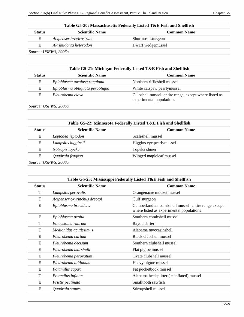
Section 316(b) Final Rule: Phase III – Regional Benefits Assessment, Part G: The Inland Region Chapter G5
G5-9
Table G5-20: Massachusetts Federally Listed T&E Fish and Shellfish Status Scientific Name Common Name
E Acipenser brevirostrum Shortnose sturgeon E Alasmidonta heterodon Dwarf wedgemussel
Source: USFWS, 2006a.
Table G5-21: Michigan Federally Listed T&E Fish and Shellfish Status Scientific Name Common Name
E Epioblasma torulosa rangiana Northern riffleshell mussel E Epioblasma obliquata perobliqua White catspaw pearlymussel E Pleurobema clava Clubshell mussel: entire range, except where listed as
experimental populations Source: USFWS, 2006a.
Table G5-22: Minnesota Federally Listed T&E Fish and Shellfish Status Scientific Name Common Name
E Leptodea leptodon Scaleshell mussel E Lampsilis higginsii Higgins eye pearlymussel E Notropis topeka Topeka shiner E Quadrula fragosa Winged mapleleaf mussel
Source: USFWS, 2006a.
Table G5-23: Mississippi Federally Listed T&E Fish and Shellfish Status Scientific Name Common Name
T Lampsilis perovalis Orangenacre mucket mussel T Acipenser oxyrinchus desotoi Gulf sturgeon E Epioblasma brevidens Cumberlandian combshell mussel: entire range except
where listed as experimental populations E Epioblasma penita Southern combshell mussel T Etheostoma rubrum Bayou darter T Medionidus acutissimus Alabama moccasinshell E Pleurobema curtum Black clubshell mussel E Pleurobema decisum Southern clubshell mussel E Pleurobema marshalli Flat pigtoe mussel E Pleurobema perovatum Ovate clubshell mussel E Pleurobema taitianum Heavy pigtoe mussel E Potamilus capax Fat pocketbook mussel T Potamilus inflatus Alabama heelsplitter ( = inflated) mussel E Pristis pectinata Smalltooth sawfish E Quadrula stapes Stirrupshell mussel
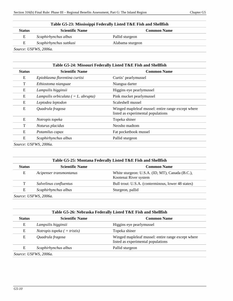
Section 316(b) Final Rule: Phase III – Regional Benefits Assessment, Part G: The Inland Region Chapter G5
G5-10
Table G5-23: Mississippi Federally Listed T&E Fish and Shellfish Status Scientific Name Common Name
E Scaphirhynchus albus Pallid sturgeon E Scaphirhynchus suttkusi Alabama sturgeon
Source: USFWS, 2006a.
Table G5-24: Missouri Federally Listed T&E Fish and Shellfish Status Scientific Name Common Name
E Epioblasma florentina curtisi Curtis’ pearlymussel T Ethiostoma nianguae Niangua darter E Lampsilis higginsii Higgins eye pearlymussel E Lampsilis orbiculata ( = L. abrupta) Pink mucket pearlymussel E Leptodea leptodon Scaleshell mussel E Quadrula fragosa Winged mapleleaf mussel: entire range except where
listed as experimental populations E Notropis topeka Topeka shiner T Noturus placidus Neosho madtom E Potamilus capax Fat pocketbook mussel E Scaphirhynchus albus Pallid sturgeon
Source: USFWS, 2006a.
Table G5-25: Montana Federally Listed T&E Fish and Shellfish Status Scientific Name Common Name
E Acipenser transmontanus White sturgeon: U.S.A. (ID, MT), Canada (B.C.), Kootenai River system
T Salvelinus confluentus Bull trout: U.S.A. (conterminous, lower 48 states) E Scaphirhynchus albus Sturgeon, pallid
Source: USFWS, 2006a.
Table G5-26: Nebraska Federally Listed T&E Fish and Shellfish Status Scientific Name Common Name
E Lampsilis higginsii Higgins eye pearlymussel E Notropis topeka ( = tristis) Topeka shiner E Quadrula fragosa Winged mapleleaf mussel: entire range except where
listed as experimental populations E Scaphirhynchus albus Pallid sturgeon
Source: USFWS, 2006a.
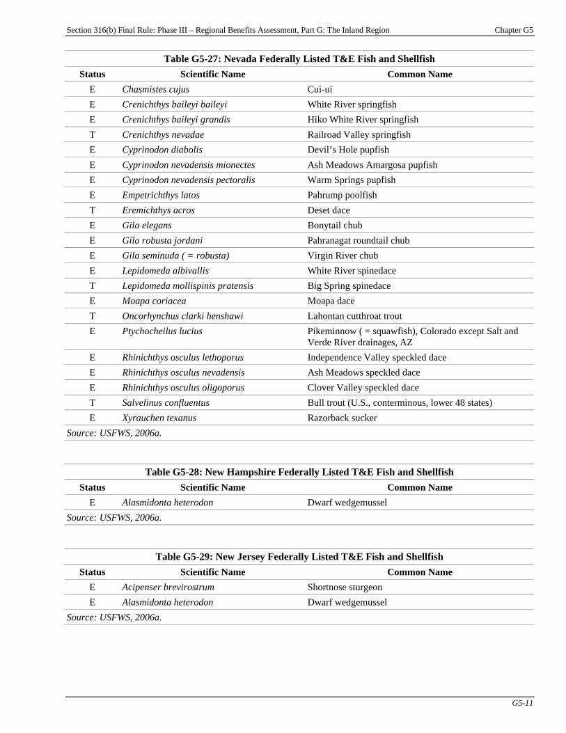
Section 316(b) Final Rule: Phase III – Regional Benefits Assessment, Part G: The Inland Region Chapter G5
G5-11
Table G5-27: Nevada Federally Listed T&E Fish and Shellfish Status Scientific Name Common Name
E Chasmistes cujus Cui-ui E Crenichthys baileyi baileyi White River springfish E Crenichthys baileyi grandis Hiko White River springfish T Crenichthys nevadae Railroad Valley springfish E Cyprinodon diabolis Devil’s Hole pupfish E Cyprinodon nevadensis mionectes Ash Meadows Amargosa pupfish E Cyprinodon nevadensis pectoralis Warm Springs pupfish E Empetrichthys latos Pahrump poolfish T Eremichthys acros Deset dace E Gila elegans Bonytail chub E Gila robusta jordani Pahranagat roundtail chub E Gila seminuda ( = robusta) Virgin River chub E Lepidomeda albivallis White River spinedace T Lepidomeda mollispinis pratensis Big Spring spinedace E Moapa coriacea Moapa dace T Oncorhynchus clarki henshawi Lahontan cutthroat trout E Ptychocheilus lucius Pikeminnow ( = squawfish), Colorado except Salt and
Verde River drainages, AZ E Rhinichthys osculus lethoporus Independence Valley speckled dace E Rhinichthys osculus nevadensis Ash Meadows speckled dace E Rhinichthys osculus oligoporus Clover Valley speckled dace T Salvelinus confluentus Bull trout (U.S., conterminous, lower 48 states) E Xyrauchen texanus Razorback sucker
Source: USFWS, 2006a.
Table G5-28: New Hampshire Federally Listed T&E Fish and Shellfish Status Scientific Name Common Name
E Alasmidonta heterodon Dwarf wedgemussel Source: USFWS, 2006a.
Table G5-29: New Jersey Federally Listed T&E Fish and Shellfish Status Scientific Name Common Name
E Acipenser brevirostrum Shortnose sturgeon E Alasmidonta heterodon Dwarf wedgemussel
Source: USFWS, 2006a.
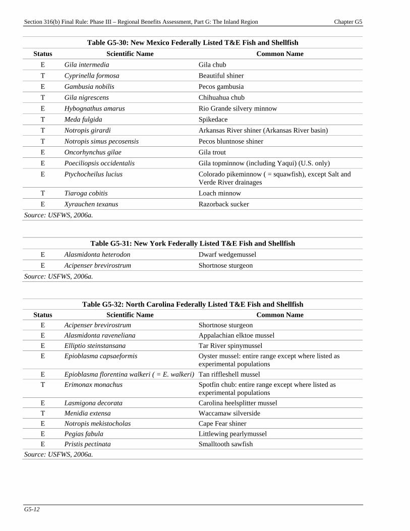
Section 316(b) Final Rule: Phase III – Regional Benefits Assessment, Part G: The Inland Region Chapter G5
G5-12
Table G5-30: New Mexico Federally Listed T&E Fish and Shellfish Status Scientific Name Common Name
E Gila intermedia Gila chub T Cyprinella formosa Beautiful shiner E Gambusia nobilis Pecos gambusia T Gila nigrescens Chihuahua chub E Hybognathus amarus Rio Grande silvery minnow T Meda fulgida Spikedace T Notropis girardi Arkansas River shiner (Arkansas River basin) T Notropis simus pecosensis Pecos bluntnose shiner E Oncorhynchus gilae Gila trout E Poeciliopsis occidentalis Gila topminnow (including Yaqui) (U.S. only) E Ptychocheilus lucius Colorado pikeminnow ( = squawfish), except Salt and
Verde River drainages T Tiaroga cobitis Loach minnow E Xyrauchen texanus Razorback sucker
Source: USFWS, 2006a.
Table G5-31: New York Federally Listed T&E Fish and Shellfish E Alasmidonta heterodon Dwarf wedgemussel E Acipenser brevirostrum Shortnose sturgeon
Source: USFWS, 2006a.
Table G5-32: North Carolina Federally Listed T&E Fish and Shellfish Status Scientific Name Common Name
E Acipenser brevirostrum Shortnose sturgeon E Alasmidonta raveneliana Appalachian elktoe mussel E Elliptio steinstansana Tar River spinymussel E Epioblasma capsaeformis Oyster mussel: entire range except where listed as
experimental populations E Epioblasma florentina walkeri ( = E. walkeri) Tan riffleshell mussel T Erimonax monachus Spotfin chub: entire range except where listed as
experimental populations E Lasmigona decorata Carolina heelsplitter mussel T Menidia extensa Waccamaw silverside E Notropis mekistocholas Cape Fear shiner E Pegias fabula Littlewing pearlymussel E Pristis pectinata Smalltooth sawfish
Source: USFWS, 2006a.
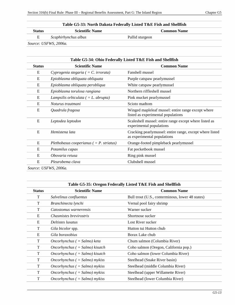
Section 316(b) Final Rule: Phase III – Regional Benefits Assessment, Part G: The Inland Region Chapter G5
G5-13
Table G5-33: North Dakota Federally Listed T&E Fish and Shellfish Status Scientific Name Common Name
E Scaphirhynchus albus Pallid sturgeon Source: USFWS, 2006a.
Table G5-34: Ohio Federally Listed T&E Fish and Shellfish Status Scientific Name Common Name
E Cyprogenia stegaria ( = C. irrorata) Fanshell mussel E Epioblasma obliquata obliquata Purple catspaw pearlymussel E Epioblasma obliquata perobliqua White catspaw pearlymussel E Epioblasma torulosa rangiana Northern riffleshell mussel E Lampsilis orbiculata ( = L. abrupta) Pink mucket pearlymussel E Noturus trautmani Scioto madtom E Quadrula fragosa Winged mapleleaf mussel: entire range except where
listed as experimental populations E Leptodea leptodon Scaleshell mussel: entire range except where listed as
experimental populations E Hemistena lata Cracking pearlymussel: entire range, except where listed
as experimental populations E Plethobasus cooperianus ( = P. striatus) Orange-footed pimpleback pearlymussel E Potamilus capax Fat pocketbook mussel E Obovaria retusa Ring pink mussel E Pleurobema clava Clubshell mussel
Source: USFWS, 2006a.
Table G5-35: Oregon Federally Listed T&E Fish and Shellfish Status Scientific Name Common Name
T Salvelinus confluentus Bull trout (U.S., conterminous, lower 48 states) T Branchinecta lynchi Vernal pool fairy shrimp T Catostomus warnerensis Warner sucker E Chasmistes brevirostris Shortnose sucker E Deltistes luxatus Lost River sucker T Gila bicolor spp. Hutton tui Hutton chub E Gila boraxobius Borax Lake chub T Oncorhynchus ( = Salmo) keta Chum salmon (Columbia River) T Oncorhynchus ( = Salmo) kisutch Coho salmon (Oregon, California pop.) T Oncorhynchus ( = Salmo) kisutch Coho salmon (lower Columbia River) T Oncorhynchus ( = Salmo) mykiss Steelhead (Snake River basin) T Oncorhynchus ( = Salmo) mykiss Steelhead (middle Columbia River) T Oncorhynchus ( = Salmo) mykiss Steelhead (upper Willamette River) T Oncorhynchus ( = Salmo) mykiss Steelhead (lower Columbia River)

Section 316(b) Final Rule: Phase III – Regional Benefits Assessment, Part G: The Inland Region Chapter G5
G5-14
Table G5-35: Oregon Federally Listed T&E Fish and Shellfish Status Scientific Name Common Name
E Oncorhynchus ( = Salmo) nerka Sockeye salmon (U.S., Snake River, ID stock wherever found)
T Oncorhynchus ( = Salmo) tshawytscha Chinook salmon (Snake River) (fall run) T Oncorhynchus ( = Salmo) tshawytscha Chinook salmon (lower Columbia River) T Oncorhynchus ( = Salmo) tshawytscha Chinook salmon (Snake River) (spring/summer run) T Oncorhynchus ( = Salmo) tshawytscha Chinook salmon (upper Willamette River) T Oncorhynchus clarki henshawi Lahontan cutthroat trout E Oregonichthys crameri Oregon chub T Rhinichthys osculus spp. Foskett dace ( = speckled Foskett)
Source: USFWS, 2006a.
Table G5-36: Pennsylvania Federally Listed T&E Fish and Shellfish Status Scientific Name Common Name
E Pleurobema clava Clubshell mussel: entire range except where listed as experimental populations
E Cyprogenia stegaria Fanshell mussel E Lampsilis abrupta Pink mucket pearlymussel E Pleurobema plenum Rough pigtoe pearlymussel E Plethobasus cooperianus Orange-foot pimpleback pearlymussel E Epioblasma torulosa rangiana Northern riffleshell mussel E Obovaria retusa Ring pink mussel E Alasmidonta heterodon Dwarf wedgemussel
Source: USFWS, 2006a.
Table G5-37: South Carolina Federally Listed T&E Fish and Shellfish Status Scientific Name Common Name
E Acipenser brevirostrum Shortnose sturgeon E Lasmigona decorata Carolina heelsplitter mussel E Pristis pectinata Smalltooth sawfish
Source: USFWS, 2006a.
Table G5-38: South Dakota Federally Listed T&E Fish and Shellfish Status Scientific Name Common Name
E Leptodea leptodon Scaleshell mussel E Notropis topeka Topeka shiner E Scaphirhynchus albus Pallid sturgeon
Source: USFWS, 2006a.

Section 316(b) Final Rule: Phase III – Regional Benefits Assessment, Part G: The Inland Region Chapter G5
G5-15
Table G5-39: Tennessee Federally Listed T&E Fish and Shellfish Status Scientific Name Common Name
T Cyprinella ( = Hybopsis) cahni Spotfin chub T Cyprinella ( = Notropis) caerulea
( = caeruleus) Blue shiner
E Etheostoma. ( = Catonotus) percnurum Duskytail darter E Etheostoma ( = Doration) spp. Bluemask ( = jewel) darter E Etheostoma ( = Nothonotus) wapiti Boulder darter T Erimystax ( = Hybopsis) cahni Slender chub T Etheostoma boschungi Slackwater darter E Hemistena ( = Lastena) lata Cracking pearlymussel: entire range except where listed
as experimental populations E Lampsilis virescens Alabama lampmussel: entire range except where listed as
experimental populations E Lampsilis abrupta ( = orbiculata) Pink mucket pearlymussel E Epioblasma othcaloogensis Southern acornshell mussel E Epioblasma torulosa gubernaculum Green blossom pearlymussel E Epioblasma turgidula Turgid blossom pearlymussel: entire range except where
listed as experimental populations E Epioblasma florentina florentina Yellow blossom pearlymussel: entire range except where
listed as experimental populations E Epioblasma obliquata obliquata Purple catspaw pearlymussel: entire range except where
listed as experimental populations E Epioblasma brevidens Cumberlandian combshell mussel: entire range except
where listed as experimental populations E Epioblasma metastriata Upland combshell mussel E Percina aurolineata Goldline darter E Alasmidonta raveneliana Appalachian elktoe mussel E Alasmidonta atropurpurea Cumberland elktoe mussel E Cyprogenia stegaria Fanshell mussel E Epioblasma capsaeformis Oyster mussel: entire range except where listed as
experimental populations E Leptodea leptodon Scaleshell mussel E Conradilla caelata Birdwing pearlymussel: entire range except where listed
as experimental populations E Dromus dromas Dromedary pearlymussel: entire range except where
listed as experimental populations E Pleurobema gibberum Cumberland pigtoe mussel E Epioblasma florentina walker ( = E. walkeri) Tan riffleshell mussel E Fusconaia cor Shiny pigtoe mussel: entire range except where listed as
experimental populations E Medionidus parvulus Coosa moccasinshell E Notropis albizonatus (cf. N. procne) Palezone shiner E Noturus baileyi Smoky madtom T Noturus flavipinnis Yellowfin madtom E Noturus stanauli Pygmy madtom
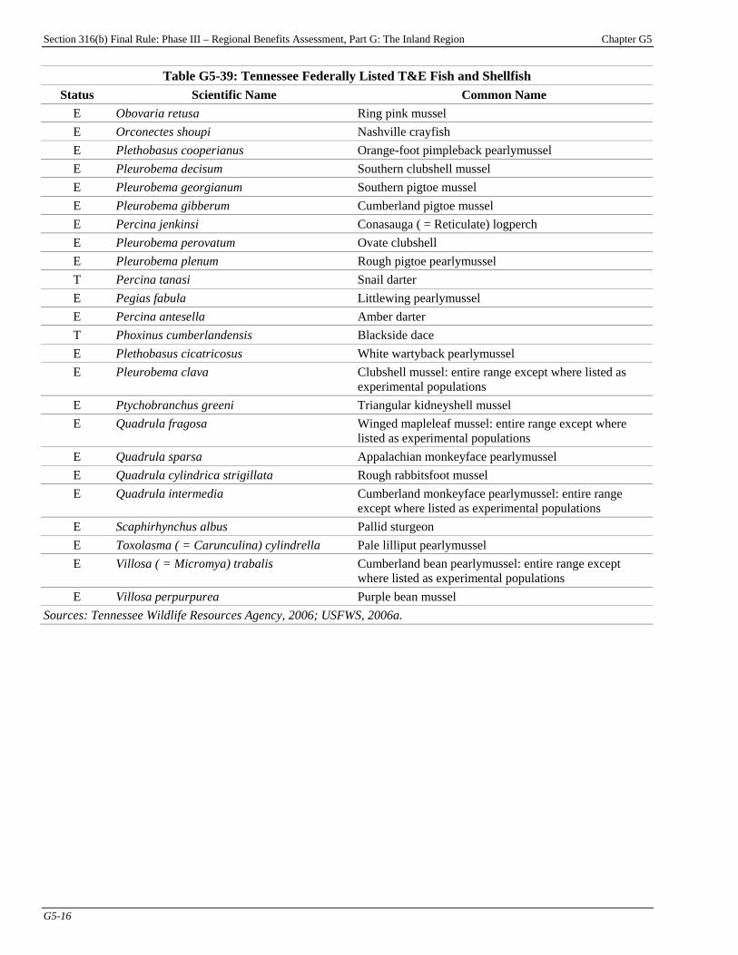
Section 316(b) Final Rule: Phase III – Regional Benefits Assessment, Part G: The Inland Region Chapter G5
G5-16
Table G5-39: Tennessee Federally Listed T&E Fish and Shellfish Status Scientific Name Common Name
E Obovaria retusa Ring pink mussel E Orconectes shoupi Nashville crayfish E Plethobasus cooperianus Orange-foot pimpleback pearlymussel E Pleurobema decisum Southern clubshell mussel E Pleurobema georgianum Southern pigtoe mussel E Pleurobema gibberum Cumberland pigtoe mussel E Percina jenkinsi Conasauga ( = Reticulate) logperch E Pleurobema perovatum Ovate clubshell E Pleurobema plenum Rough pigtoe pearlymussel T Percina tanasi Snail darter E Pegias fabula Littlewing pearlymussel E Percina antesella Amber darter T Phoxinus cumberlandensis Blackside dace E Plethobasus cicatricosus White wartyback pearlymussel E Pleurobema clava Clubshell mussel: entire range except where listed as
experimental populations E Ptychobranchus greeni Triangular kidneyshell mussel E Quadrula fragosa Winged mapleleaf mussel: entire range except where
listed as experimental populations E Quadrula sparsa Appalachian monkeyface pearlymussel E Quadrula cylindrica strigillata Rough rabbitsfoot mussel E Quadrula intermedia Cumberland monkeyface pearlymussel: entire range
except where listed as experimental populations E Scaphirhynchus albus Pallid sturgeon E Toxolasma ( = Carunculina) cylindrella Pale lilliput pearlymussel E Villosa ( = Micromya) trabalis Cumberland bean pearlymussel: entire range except
where listed as experimental populations E Villosa perpurpurea Purple bean mussel
Sources: Tennessee Wildlife Resources Agency, 2006; USFWS, 2006a.
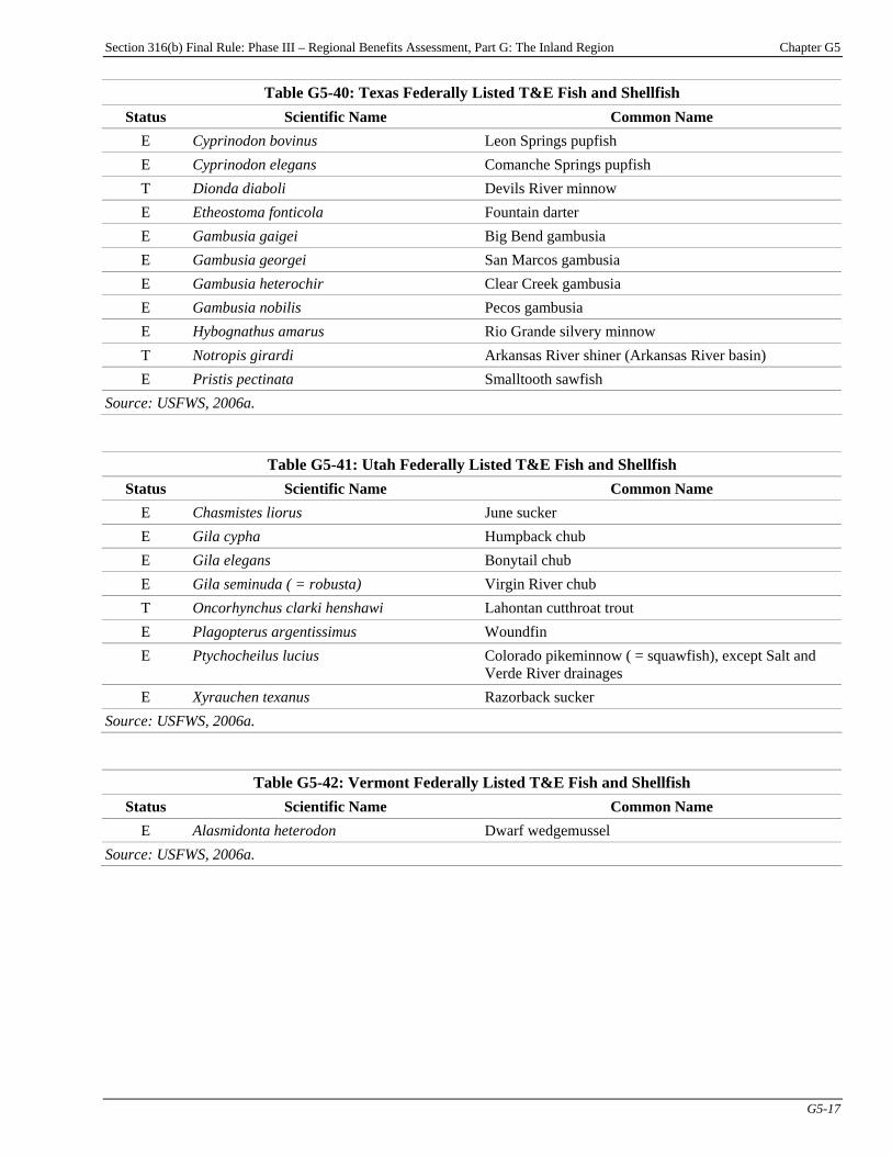
Section 316(b) Final Rule: Phase III – Regional Benefits Assessment, Part G: The Inland Region Chapter G5
G5-17
Table G5-40: Texas Federally Listed T&E Fish and Shellfish Status Scientific Name Common Name
E Cyprinodon bovinus Leon Springs pupfish E Cyprinodon elegans Comanche Springs pupfish T Dionda diaboli Devils River minnow E Etheostoma fonticola Fountain darter E Gambusia gaigei Big Bend gambusia E Gambusia georgei San Marcos gambusia E Gambusia heterochir Clear Creek gambusia E Gambusia nobilis Pecos gambusia E Hybognathus amarus Rio Grande silvery minnow T Notropis girardi Arkansas River shiner (Arkansas River basin) E Pristis pectinata Smalltooth sawfish
Source: USFWS, 2006a.
Table G5-41: Utah Federally Listed T&E Fish and Shellfish Status Scientific Name Common Name
E Chasmistes liorus June sucker E Gila cypha Humpback chub E Gila elegans Bonytail chub E Gila seminuda ( = robusta) Virgin River chub T Oncorhynchus clarki henshawi Lahontan cutthroat trout E Plagopterus argentissimus Woundfin E Ptychocheilus lucius Colorado pikeminnow ( = squawfish), except Salt and
Verde River drainages E Xyrauchen texanus Razorback sucker
Source: USFWS, 2006a.
Table G5-42: Vermont Federally Listed T&E Fish and Shellfish Status Scientific Name Common Name
E Alasmidonta heterodon Dwarf wedgemussel Source: USFWS, 2006a.
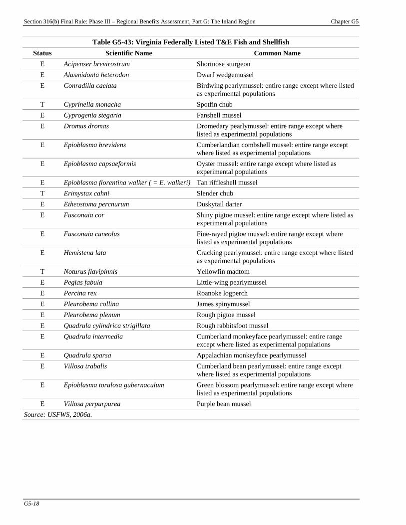
Section 316(b) Final Rule: Phase III – Regional Benefits Assessment, Part G: The Inland Region Chapter G5
G5-18
Table G5-43: Virginia Federally Listed T&E Fish and Shellfish Status Scientific Name Common Name
E Acipenser brevirostrum Shortnose sturgeon E Alasmidonta heterodon Dwarf wedgemussel E Conradilla caelata Birdwing pearlymussel: entire range except where listed
as experimental populations T Cyprinella monacha Spotfin chub E Cyprogenia stegaria Fanshell mussel E Dromus dromas Dromedary pearlymussel: entire range except where
listed as experimental populations E Epioblasma brevidens Cumberlandian combshell mussel: entire range except
where listed as experimental populations E Epioblasma capsaeformis Oyster mussel: entire range except where listed as
experimental populations E Epioblasma florentina walker ( = E. walkeri) Tan riffleshell mussel T Erimystax cahni Slender chub E Etheostoma percnurum Duskytail darter E Fusconaia cor Shiny pigtoe mussel: entire range except where listed as
experimental populations E Fusconaia cuneolus Fine-rayed pigtoe mussel: entire range except where
listed as experimental populations E Hemistena lata Cracking pearlymussel: entire range except where listed
as experimental populations T Noturus flavipinnis Yellowfin madtom E Pegias fabula Little-wing pearlymussel E Percina rex Roanoke logperch E Pleurobema collina James spinymussel E Pleurobema plenum Rough pigtoe mussel E Quadrula cylindrica strigillata Rough rabbitsfoot mussel E Quadrula intermedia Cumberland monkeyface pearlymussel: entire range
except where listed as experimental populations E Quadrula sparsa Appalachian monkeyface pearlymussel E Villosa trabalis Cumberland bean pearlymussel: entire range except
where listed as experimental populations E Epioblasma torulosa gubernaculum Green blossom pearlymussel: entire range except where
listed as experimental populations E Villosa perpurpurea Purple bean mussel
Source: USFWS, 2006a.
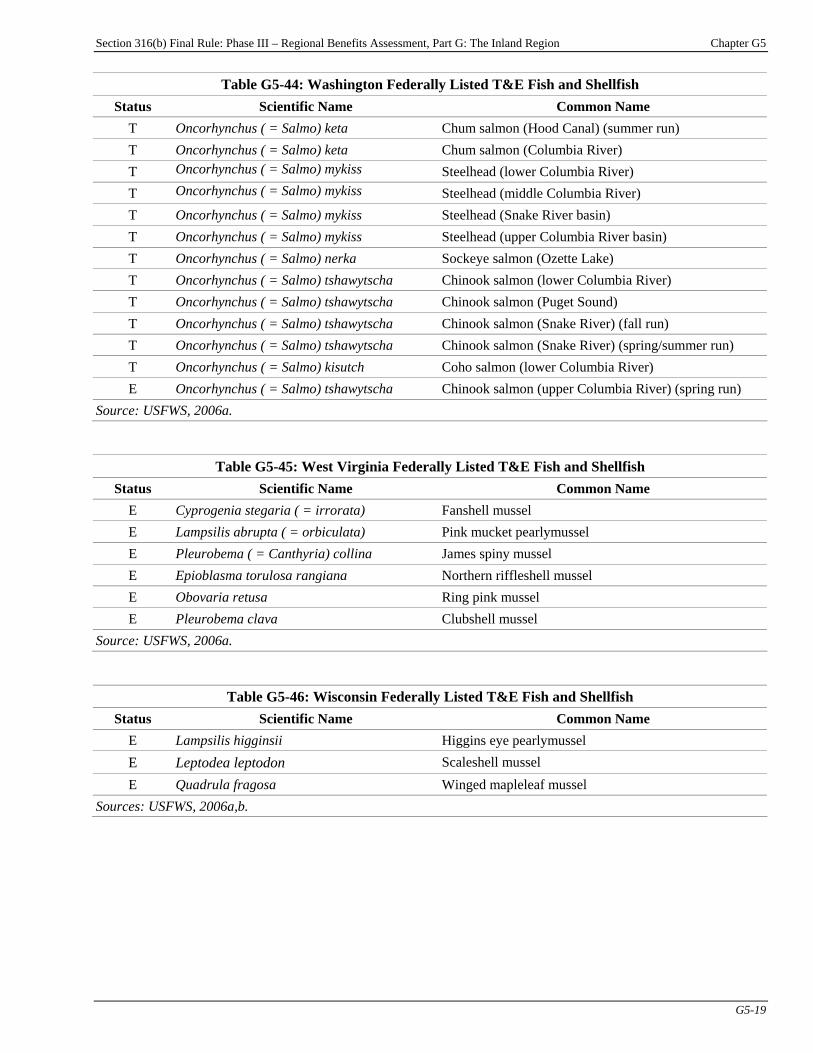
Section 316(b) Final Rule: Phase III – Regional Benefits Assessment, Part G: The Inland Region Chapter G5
G5-19
Table G5-44: Washington Federally Listed T&E Fish and Shellfish Status Scientific Name Common Name
T Oncorhynchus ( = Salmo) keta Chum salmon (Hood Canal) (summer run) T Oncorhynchus ( = Salmo) keta Chum salmon (Columbia River) T Oncorhynchus ( = Salmo) mykiss Steelhead (lower Columbia River) T Oncorhynchus ( = Salmo) mykiss Steelhead (middle Columbia River) T Oncorhynchus ( = Salmo) mykiss Steelhead (Snake River basin) T Oncorhynchus ( = Salmo) mykiss Steelhead (upper Columbia River basin) T Oncorhynchus ( = Salmo) nerka Sockeye salmon (Ozette Lake) T Oncorhynchus ( = Salmo) tshawytscha Chinook salmon (lower Columbia River) T Oncorhynchus ( = Salmo) tshawytscha Chinook salmon (Puget Sound) T Oncorhynchus ( = Salmo) tshawytscha Chinook salmon (Snake River) (fall run) T Oncorhynchus ( = Salmo) tshawytscha Chinook salmon (Snake River) (spring/summer run) T Oncorhynchus ( = Salmo) kisutch Coho salmon (lower Columbia River) E Oncorhynchus ( = Salmo) tshawytscha Chinook salmon (upper Columbia River) (spring run)
Source: USFWS, 2006a.
Table G5-45: West Virginia Federally Listed T&E Fish and Shellfish Status Scientific Name Common Name
E Cyprogenia stegaria ( = irrorata) Fanshell mussel E Lampsilis abrupta ( = orbiculata) Pink mucket pearlymussel E Pleurobema ( = Canthyria) collina James spiny mussel E Epioblasma torulosa rangiana Northern riffleshell mussel E Obovaria retusa Ring pink mussel E Pleurobema clava Clubshell mussel
Source: USFWS, 2006a.
Table G5-46: Wisconsin Federally Listed T&E Fish and Shellfish Status Scientific Name Common Name
E Lampsilis higginsii Higgins eye pearlymussel E Leptodea leptodon Scaleshell mussel E Quadrula fragosa Winged mapleleaf mussel
Sources: USFWS, 2006a,b.
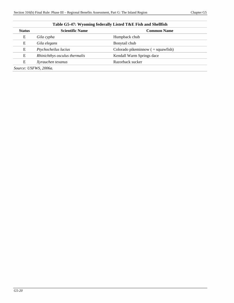
Section 316(b) Final Rule: Phase III – Regional Benefits Assessment, Part G: The Inland Region Chapter G5
G5-20
Table G5-47: Wyoming federally Listed T&E Fish and Shellfish Status Scientific Name Common Name
E Gila cypha Humpback chub E Gila elegans Bonytail chub E Ptychocheilus lucius Colorado pikeminnow ( = squawfish) E Rhinichthys osculus thermalis Kendall Warm Springs dace E Xyrauchen texanus Razorback sucker
Source: USFWS, 2006a.

Section 316(b) Final Rule: Phase III – Regional Benefits Assessment
Part H: South Atlantic

Section 316(b) Final Rule: Phase III – Regional Benefits Assessment, Part H: South Atlantic Chapter H1
H1-1
Chapter H1: Background Introduction This chapter presents an overview of the potential Phase III existing facilities in the South Atlantic study region and summarizes their key cooling water and compliance characteristics. For further discussion of the technical and compliance characteristics of potential Phase III existing facilities, refer to the Economic Analysis for the Final Section 316(b) Rule for Phase III Facilities and the Technical Development Document for the Final Section 316(b) Rule for Phase III Facilities (U.S. EPA, 2006a,c).
Chapter Contents H1-1 Facility Characteristics..................................H1-1
H1-1 Facility Characteristics The South Atlantic Regional Study includes one sample facility that is potentially subject to the national standards for Phase III existing facilities. Figure H1-1 presents a map of this manufacturing facility. Industry-wide, this one sample facility represents four manufacturing facilities.PF
1FP
P
1P EPA applied sample weights to the survey respondents to account for non-sampled facilities and facilities that did
not respond to the survey. For more information on EPA’s 2000 Section 316(b) Industry Survey, please refer to the Information Collection Request (U.S. EPA, 2000b).

Section 316(b) Final Rule: Phase III – Regional Benefits Assessment, Part H: South Atlantic Chapter H1
H1-2
Figure H1-1: Potential Existing Phase III Facilities in the South Atlantic Regional StudyP
aP
P
aP The map includes locations of sample facilities only.
Source: U.S. EPA analysis for this report.

Section 316(b) Final Rule: Phase III – Regional Benefits Assessment, Part H: South Atlantic Chapter H1
H1-3
Table H1-1 summarizes key technical and compliance characteristics for all potentially regulated Phase III existing facilities in the South Atlantic study region for the regulatory options considered by EPA for this rule (the “50 MGD for All Waterbodies” option, the “200 MGD for All Waterbodies” option, and the “100 MGD for Certain Waterbodies” option). Facilities with a design intake flow below the three applicability thresholds would be subject to permitting based on best professional judgment and are excluded from EPA’s analyses.PF
2FP Therefore,
a different number of facilities is affected under each option. Table H1-1 shows that four Phase III existing facilities in the South Atlantic study region would potentially be subject to the national requirements. Under the “50 MGD for All Waterbodies” option, the most inclusive of the regulatory options, no facilities would be subject to the national requirements for Phase III existing facilities. Under the less inclusive “200 MGD for All Waterbodies” and “100 MGD for Certain Waterbodies” options, no facilities would be subject to the nation requirements. This facility in the South Atlantic study region does not have a recirculating system in the baseline. Data on design intake flow for the South Atlantic study facilities have been withheld due to data confidentiality reasons.
Table H1-1: Technical and Compliance Characteristics of Existing Phase III Facilities (sample-weighted) Regulatory Options All Potentially
Regulated Facilities
50 MGD All
200 MGD All
100 MGD CWB
Total Number of Facilities (sample-weighted) 4 - - - Number of Facilities with Recirculating System in Baseline - - - - Design Intake Flow (MGD) wP
aP - - -
Number of Facilities by Compliance Response New larger intake structure with fine mesh and fish H&R - - - - Fine mesh traveling screens with fish H&R - - - - Passive fine mesh screens - - - - None 4 - - -
Compliance Cost, Discounted at 3%P
bP $0.68 $0.00 $0.00 $0.00
Compliance Cost, Discounted at 7%P
bP $0.63 $0.00 $0.00 $0.00
P
aP Data withheld because of confidentiality reasons.
P
bP Annualized pre-tax compliance cost (2004$, millions).
Sources: U.S. EPA, 2000b; U.S. EPA analysis for this report.
P
2P Also excluded are facilities that are estimated to be baseline closures. For additional information on EPA’s
baseline closure analyses, please refer to the Economic Analysis for the Final Section 316(b) Rule for Phase III Facilities (U.S. EPA, 2006a).
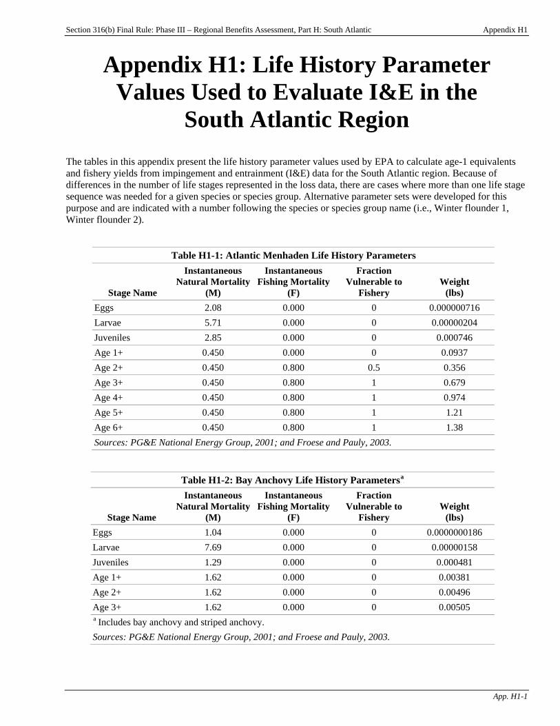
Section 316(b) Final Rule: Phase III – Regional Benefits Assessment, Part H: South Atlantic Appendix H1
App. H1-1
Appendix H1: Life History Parameter Values Used to Evaluate I&E in the
South Atlantic Region The tables in this appendix present the life history parameter values used by EPA to calculate age-1 equivalents and fishery yields from impingement and entrainment (I&E) data for the South Atlantic region. Because of differences in the number of life stages represented in the loss data, there are cases where more than one life stage sequence was needed for a given species or species group. Alternative parameter sets were developed for this purpose and are indicated with a number following the species or species group name (i.e., Winter flounder 1, Winter flounder 2).
Table H1-1: Atlantic Menhaden Life History Parameters
Stage Name
Instantaneous Natural Mortality
(M)
Instantaneous Fishing Mortality
(F)
Fraction Vulnerable to
Fishery Weight
(lbs) Eggs 2.08 0.000 0 0.000000716 Larvae 5.71 0.000 0 0.00000204 Juveniles 2.85 0.000 0 0.000746 Age 1+ 0.450 0.000 0 0.0937 Age 2+ 0.450 0.800 0.5 0.356 Age 3+ 0.450 0.800 1 0.679 Age 4+ 0.450 0.800 1 0.974 Age 5+ 0.450 0.800 1 1.21 Age 6+ 0.450 0.800 1 1.38 Sources: PG&E National Energy Group, 2001; and Froese and Pauly, 2003.
Table H1-2: Bay Anchovy Life History ParametersP
aP
Stage Name
Instantaneous Natural Mortality
(M)
Instantaneous Fishing Mortality
(F)
Fraction Vulnerable to
Fishery Weight
(lbs) Eggs 1.04 0.000 0 0.0000000186 Larvae 7.69 0.000 0 0.00000158 Juveniles 1.29 0.000 0 0.000481 Age 1+ 1.62 0.000 0 0.00381 Age 2+ 1.62 0.000 0 0.00496 Age 3+ 1.62 0.000 0 0.00505 P
a PIncludes bay anchovy and striped anchovy.
Sources: PG&E National Energy Group, 2001; and Froese and Pauly, 2003.
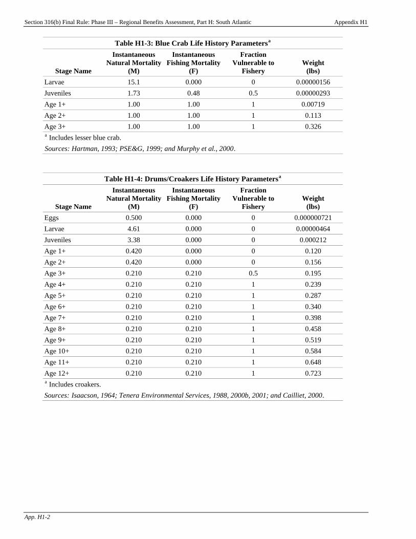
Section 316(b) Final Rule: Phase III – Regional Benefits Assessment, Part H: South Atlantic Appendix H1
App. H1-2
Table H1-3: Blue Crab Life History ParametersP
aP
Stage Name
Instantaneous Natural Mortality
(M)
Instantaneous Fishing Mortality
(F)
Fraction Vulnerable to
Fishery Weight
(lbs) Larvae 15.1 0.000 0 0.00000156 Juveniles 1.73 0.48 0.5 0.00000293 Age 1+ 1.00 1.00 1 0.00719 Age 2+ 1.00 1.00 1 0.113 Age 3+ 1.00 1.00 1 0.326 P
aP Includes lesser blue crab.
TSources: Hartman, 1993; PSE&G, 1999; and Murphy et al., 2000T.
Table H1-4: Drums/Croakers Life History ParametersP
aP
Stage Name
Instantaneous Natural Mortality
(M)
Instantaneous Fishing Mortality
(F)
Fraction Vulnerable to
Fishery Weight
(lbs) Eggs 0.500 0.000 0 0.000000721 Larvae 4.61 0.000 0 0.00000464 Juveniles 3.38 0.000 0 0.000212 Age 1+ 0.420 0.000 0 0.120 Age 2+ 0.420 0.000 0 0.156 Age 3+ 0.210 0.210 0.5 0.195 Age 4+ 0.210 0.210 1 0.239 Age 5+ 0.210 0.210 1 0.287 Age 6+ 0.210 0.210 1 0.340 Age 7+ 0.210 0.210 1 0.398 Age 8+ 0.210 0.210 1 0.458 Age 9+ 0.210 0.210 1 0.519 Age 10+ 0.210 0.210 1 0.584 Age 11+ 0.210 0.210 1 0.648 Age 12+ 0.210 0.210 1 0.723 P
aP Includes croakers.
Sources: TIsaacson, 1964; Tenera Environmental Services, 1988, 2000b, 2001; and Cailliet, 2000T.
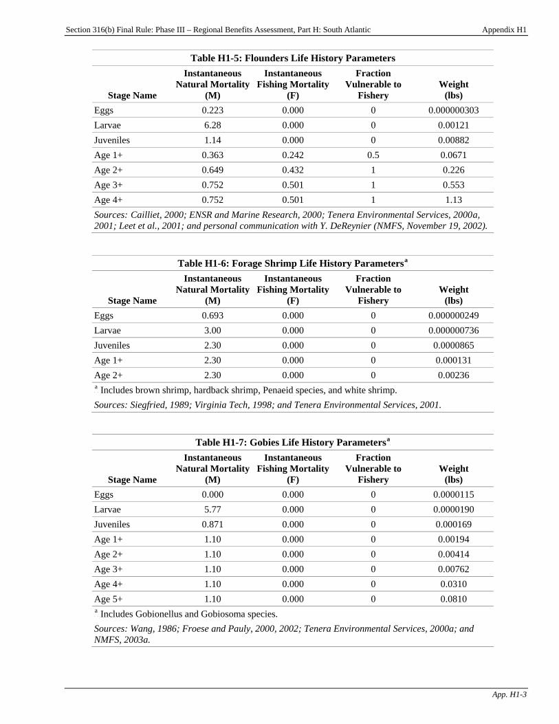
Section 316(b) Final Rule: Phase III – Regional Benefits Assessment, Part H: South Atlantic Appendix H1
App. H1-3
Table H1-5: Flounders Life History Parameters
Stage Name
Instantaneous Natural Mortality
(M)
Instantaneous Fishing Mortality
(F)
Fraction Vulnerable to
Fishery Weight
(lbs) Eggs 0.223 0.000 0 0.000000303 Larvae 6.28 0.000 0 0.00121 Juveniles 1.14 0.000 0 0.00882 Age 1+ 0.363 0.242 0.5 0.0671 Age 2+ 0.649 0.432 1 0.226 Age 3+ 0.752 0.501 1 0.553 Age 4+ 0.752 0.501 1 1.13 Sources:T Cailliet, 2000; ENSR and Marine Research, 2000; Tenera Environmental Services, 2000Ta, 2001; Leet et al., 2001; and personal communication with Y. DeReynier (NMFS, November 19, 2002).
Table H1-6: Forage Shrimp Life History ParametersP
aP
Stage Name
Instantaneous Natural Mortality
(M)
Instantaneous Fishing Mortality
(F)
Fraction Vulnerable to
Fishery Weight
(lbs) Eggs 0.693 0.000 0 0.000000249 Larvae 3.00 0.000 0 0.000000736 Juveniles 2.30 0.000 0 0.0000865 Age 1+ 2.30 0.000 0 0.000131 Age 2+ 2.30 0.000 0 0.00236 P
aP Includes brown shrimp, hardback shrimp, Penaeid species, and white shrimp.
Sources: Siegfried, 1989; Virginia Tech, 1998; and Tenera Environmental Services, 2001.
Table H1-7: Gobies Life History ParametersP
aP
Stage Name
Instantaneous Natural Mortality
(M)
Instantaneous Fishing Mortality
(F)
Fraction Vulnerable to
Fishery Weight
(lbs) Eggs 0.000 0.000 0 0.0000115 Larvae 5.77 0.000 0 0.0000190 Juveniles 0.871 0.000 0 0.000169 Age 1+ 1.10 0.000 0 0.00194 Age 2+ 1.10 0.000 0 0.00414 Age 3+ 1.10 0.000 0 0.00762 Age 4+ 1.10 0.000 0 0.0310 Age 5+ 1.10 0.000 0 0.0810 P
aP Includes Gobionellus and Gobiosoma species.
Sources: Wang, 1986; Froese and Pauly, 2000, 2002; Tenera Environmental Services, 2000a; and NMFS, 2003a.
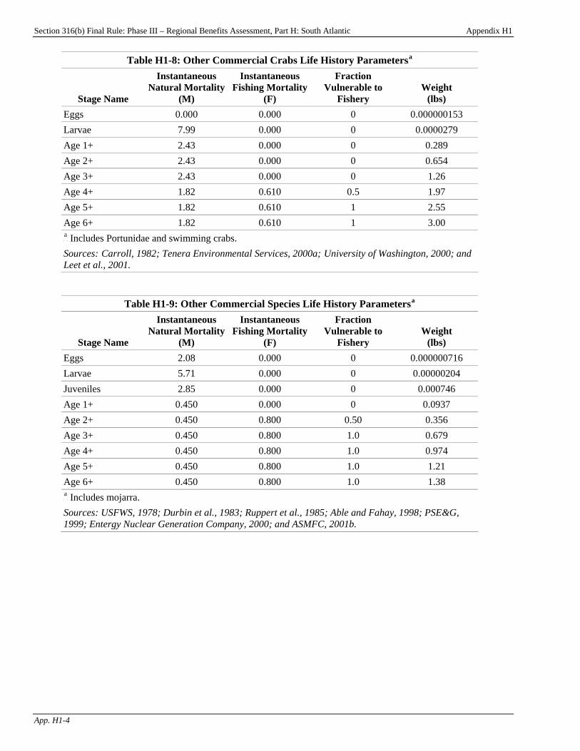
Section 316(b) Final Rule: Phase III – Regional Benefits Assessment, Part H: South Atlantic Appendix H1
App. H1-4
Table H1-8: Other Commercial Crabs Life History ParametersP
aP
Stage Name
Instantaneous Natural Mortality
(M)
Instantaneous Fishing Mortality
(F)
Fraction Vulnerable to
Fishery Weight
(lbs) Eggs 0.000 0.000 0 0.000000153 Larvae 7.99 0.000 0 0.0000279 Age 1+ 2.43 0.000 0 0.289 Age 2+ 2.43 0.000 0 0.654 Age 3+ 2.43 0.000 0 1.26 Age 4+ 1.82 0.610 0.5 1.97 Age 5+ 1.82 0.610 1 2.55 Age 6+ 1.82 0.610 1 3.00 P
aP Includes Portunidae and swimming crabs.
Sources: TCarroll, 1982; Tenera Environmental Services, 2000a; TUniversity of Washington, 2000; and Leet et al., 2001.
Table H1-9: Other Commercial Species Life History ParametersP
aP
Stage Name
Instantaneous Natural Mortality
(M)
Instantaneous Fishing Mortality
(F)
Fraction Vulnerable to
Fishery Weight
(lbs) Eggs 2.08 0.000 0 0.000000716 Larvae 5.71 0.000 0 0.00000204 Juveniles 2.85 0.000 0 0.000746 Age 1+ 0.450 0.000 0 0.0937 Age 2+ 0.450 0.800 0.50 0.356 Age 3+ 0.450 0.800 1.0 0.679 Age 4+ 0.450 0.800 1.0 0.974 Age 5+ 0.450 0.800 1.0 1.21 Age 6+ 0.450 0.800 1.0 1.38 P
aP Includes mojarra.
Sources: USFWS, 1978; Durbin et al., 1983; Ruppert et al., 1985; Able and Fahay, 1998; PSE&G, 1999; Entergy Nuclear Generation Company, 2000; and ASMFC, 2001b.
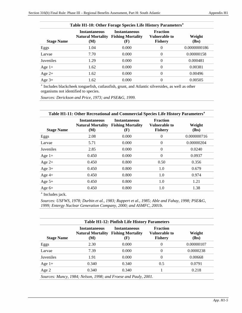
Section 316(b) Final Rule: Phase III – Regional Benefits Assessment, Part H: South Atlantic Appendix H1
App. H1-5
Table H1-10: Other Forage Species Life History ParametersP
aP
Stage Name
Instantaneous Natural Mortality
(M)
Instantaneous Fishing Mortality
(F)
Fraction Vulnerable to
Fishery Weight
(lbs) Eggs 1.04 0.000 0 0.0000000186 Larvae 7.70 0.000 0 0.00000158 Juveniles 1.29 0.000 0 0.000481 Age 1+ 1.62 0.000 0 0.00381 Age 2+ 1.62 0.000 0 0.00496 Age 3+ 1.62 0.000 0 0.00505 P
aP Includes blackcheek tonguefish, cutlassfish, grunt, and Atlantic silversides, as well as other
organisms not identified to species. Sources: Derickson and Price, 1973; and PSE&G, 1999.
Table H1-11: Other Recreational and Commercial Species Life History ParametersP
aP
Stage Name
Instantaneous Natural Mortality
(M)
Instantaneous Fishing Mortality
(F)
Fraction Vulnerable to
Fishery Weight
(lbs) Eggs 2.08 0.000 0 0.000000716 Larvae 5.71 0.000 0 0.00000204 Juveniles 2.85 0.000 0 0.0240 Age 1+ 0.450 0.000 0 0.0937 Age 2+ 0.450 0.800 0.50 0.356 Age 3+ 0.450 0.800 1.0 0.679 Age 4+ 0.450 0.800 1.0 0.974 Age 5+ 0.450 0.800 1.0 1.21 Age 6+ 0.450 0.800 1.0 1.38 P
aP Includes jack.
Sources: USFWS, 1978; Durbin et al., 1983; Ruppert et al., 1985; Able and Fahay, 1998; PSE&G, 1999; Entergy Nuclear Generation Company, 2000; and ASMFC, 2001b.
Table H1-12: Pinfish Life History Parameters
Stage Name
Instantaneous Natural Mortality
(M)
Instantaneous Fishing Mortality
(F)
Fraction Vulnerable to
Fishery Weight
(lbs) Eggs 2.30 0.000 0 0.00000107 Larvae 7.39 0.000 0 0.0000238 Juveniles 1.91 0.000 0 0.00668 Age 1+ 0.340 0.340 0.5 0.0791 Age 2 0.340 0.340 1 0.218 Sources: Muncy, 1984; Nelson, 1998; and Froese and Pauly, 2001.
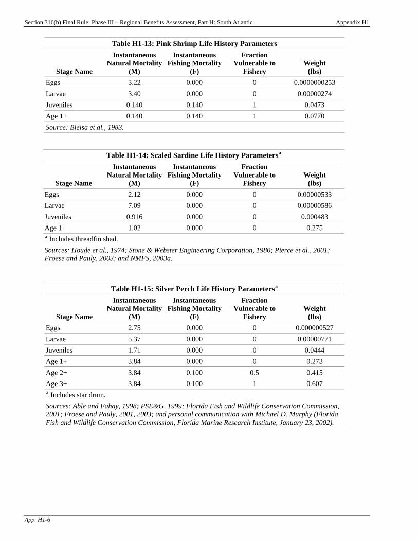
Section 316(b) Final Rule: Phase III – Regional Benefits Assessment, Part H: South Atlantic Appendix H1
App. H1-6
Table H1-13: Pink Shrimp Life History Parameters
Stage Name
Instantaneous Natural Mortality
(M)
Instantaneous Fishing Mortality
(F)
Fraction Vulnerable to
Fishery Weight
(lbs) Eggs 3.22 0.000 0 0.0000000253 Larvae 3.40 0.000 0 0.00000274 Juveniles 0.140 0.140 1 0.0473 Age 1+ 0.140 0.140 1 0.0770 Source: Bielsa et al., 1983.
Table H1-14: Scaled Sardine Life History ParametersP
aP
Stage Name
Instantaneous Natural Mortality
(M)
Instantaneous Fishing Mortality
(F)
Fraction Vulnerable to
Fishery Weight
(lbs) Eggs 2.12 0.000 0 0.00000533 Larvae 7.09 0.000 0 0.00000586 Juveniles 0.916 0.000 0 0.000483 Age 1+ 1.02 0.000 0 0.275 P
aP Includes threadfin shad.
Sources: Houde et al., 1974; Stone & Webster Engineering Corporation, 1980; Pierce et al., 2001; Froese and Pauly, 2003; and NMFS, 2003a.
Table H1-15: Silver Perch Life History ParametersP
aP
Stage Name
Instantaneous Natural Mortality
(M)
Instantaneous Fishing Mortality
(F)
Fraction Vulnerable to
Fishery Weight
(lbs) Eggs 2.75 0.000 0 0.000000527 Larvae 5.37 0.000 0 0.00000771 Juveniles 1.71 0.000 0 0.0444 Age 1+ 3.84 0.000 0 0.273 Age 2+ 3.84 0.100 0.5 0.415 Age 3+ 3.84 0.100 1 0.607 P
aP Includes star drum.
Sources: Able and Fahay, 1998; PSE&G, 1999; Florida Fish and Wildlife Conservation Commission, 2001; Froese and Pauly, 2001, 2003; and personal communication with Michael D. Murphy (Florida Fish and Wildlife Conservation Commission, Florida Marine Research Institute, January 23, 2002).
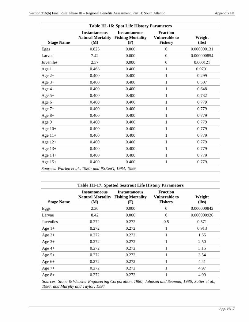
Section 316(b) Final Rule: Phase III – Regional Benefits Assessment, Part H: South Atlantic Appendix H1
App. H1-7
Table H1-16: Spot Life History Parameters
Stage Name
Instantaneous Natural Mortality
(M)
Instantaneous Fishing Mortality
(F)
Fraction Vulnerable to
Fishery Weight
(lbs) Eggs 0.825 0.000 0 0.000000131 Larvae 7.42 0.000 0 0.000000854 Juveniles 2.57 0.000 0 0.000121 Age 1+ 0.463 0.400 1 0.0791 Age 2+ 0.400 0.400 1 0.299 Age 3+ 0.400 0.400 1 0.507 Age 4+ 0.400 0.400 1 0.648 Age 5+ 0.400 0.400 1 0.732 Age 6+ 0.400 0.400 1 0.779 Age 7+ 0.400 0.400 1 0.779 Age 8+ 0.400 0.400 1 0.779 Age 9+ 0.400 0.400 1 0.779 Age 10+ 0.400 0.400 1 0.779 Age 11+ 0.400 0.400 1 0.779 Age 12+ 0.400 0.400 1 0.779 Age 13+ 0.400 0.400 1 0.779 Age 14+ 0.400 0.400 1 0.779 Age 15+ 0.400 0.400 1 0.779 Sources: Warlen et al., 1980; and PSE&G, 1984, 1999.
Table H1-17: Spotted Seatrout Life History Parameters
Stage Name
Instantaneous Natural Mortality
(M)
Instantaneous Fishing Mortality
(F)
Fraction Vulnerable to
Fishery Weight
(lbs) Eggs 2.30 0.000 0 0.000000842 Larvae 8.42 0.000 0 0.000000926 Juveniles 0.272 0.272 0.5 0.571 Age 1+ 0.272 0.272 1 0.913 Age 2+ 0.272 0.272 1 1.55 Age 3+ 0.272 0.272 1 2.50 Age 4+ 0.272 0.272 1 3.15 Age 5+ 0.272 0.272 1 3.54 Age 6+ 0.272 0.272 1 4.41 Age 7+ 0.272 0.272 1 4.97 Age 8+ 0.272 0.272 1 4.99 Sources: Stone & Webster Engineering Corporation, 1980; Johnson and Seaman, 1986; Sutter et al., 1986; and Murphy and Taylor, 1994.
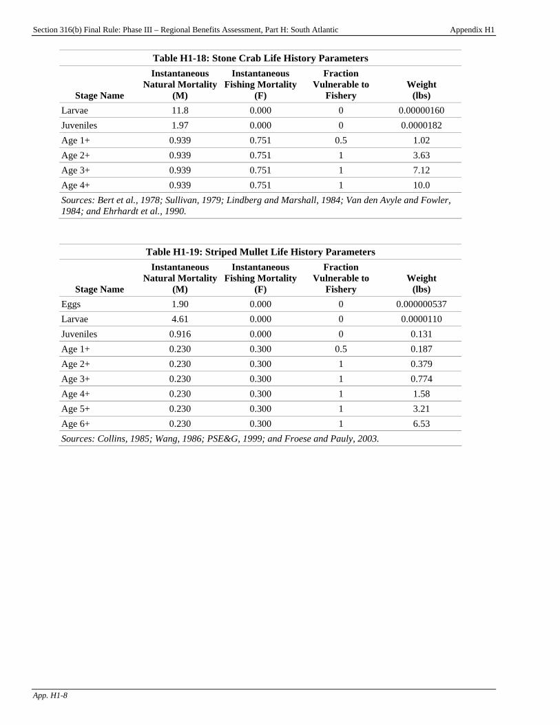
Section 316(b) Final Rule: Phase III – Regional Benefits Assessment, Part H: South Atlantic Appendix H1
App. H1-8
Table H1-18: Stone Crab Life History Parameters
Stage Name
Instantaneous Natural Mortality
(M)
Instantaneous Fishing Mortality
(F)
Fraction Vulnerable to
Fishery Weight
(lbs) Larvae 11.8 0.000 0 0.00000160 Juveniles 1.97 0.000 0 0.0000182 Age 1+ 0.939 0.751 0.5 1.02 Age 2+ 0.939 0.751 1 3.63 Age 3+ 0.939 0.751 1 7.12 Age 4+ 0.939 0.751 1 10.0 Sources: Bert et al., 1978; Sullivan, 1979; Lindberg and Marshall, 1984; Van den Avyle and Fowler, 1984; and Ehrhardt et al., 1990.
Table H1-19: Striped Mullet Life History Parameters
Stage Name
Instantaneous Natural Mortality
(M)
Instantaneous Fishing Mortality
(F)
Fraction Vulnerable to
Fishery Weight
(lbs) Eggs 1.90 0.000 0 0.000000537 Larvae 4.61 0.000 0 0.0000110 Juveniles 0.916 0.000 0 0.131 Age 1+ 0.230 0.300 0.5 0.187 Age 2+ 0.230 0.300 1 0.379 Age 3+ 0.230 0.300 1 0.774 Age 4+ 0.230 0.300 1 1.58 Age 5+ 0.230 0.300 1 3.21 Age 6+ 0.230 0.300 1 6.53 Sources: Collins, 1985; Wang, 1986; PSE&G, 1999; and Froese and Pauly, 2003.
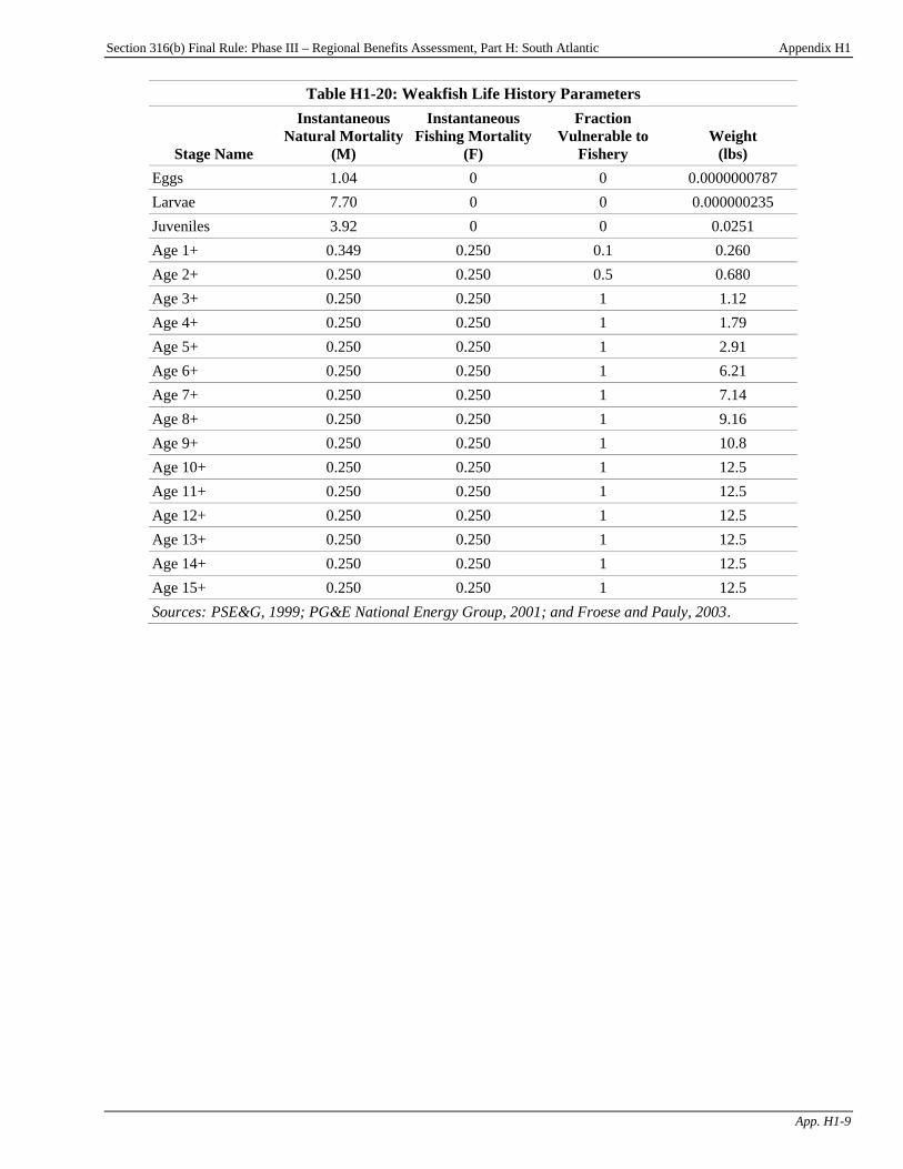
Section 316(b) Final Rule: Phase III – Regional Benefits Assessment, Part H: South Atlantic Appendix H1
App. H1-9
Table H1-20: Weakfish Life History Parameters
Stage Name
Instantaneous Natural Mortality
(M)
Instantaneous Fishing Mortality
(F)
Fraction Vulnerable to
Fishery Weight
(lbs) Eggs 1.04 0 0 0.0000000787 Larvae 7.70 0 0 0.000000235 Juveniles 3.92 0 0 0.0251 Age 1+ 0.349 0.250 0.1 0.260 Age 2+ 0.250 0.250 0.5 0.680 Age 3+ 0.250 0.250 1 1.12 Age 4+ 0.250 0.250 1 1.79 Age 5+ 0.250 0.250 1 2.91 Age 6+ 0.250 0.250 1 6.21 Age 7+ 0.250 0.250 1 7.14 Age 8+ 0.250 0.250 1 9.16 Age 9+ 0.250 0.250 1 10.8 Age 10+ 0.250 0.250 1 12.5 Age 11+ 0.250 0.250 1 12.5 Age 12+ 0.250 0.250 1 12.5 Age 13+ 0.250 0.250 1 12.5 Age 14+ 0.250 0.250 1 12.5 Age 15+ 0.250 0.250 1 12.5 Sources:T PSE&G, 1999; PG&E National Energy Group, 2001; and Froese and Pauly, 2003T.
Section 316(b) Final Rule: Phase III – Regional Benefits Assessment, Part H: South Atlantic Chapter H2
H2-1
Chapter H2: Evaluation of Impingement and Entrainment in the South Atlantic Region
Background: South Atlantic Marine Fisheries Among the species that are vulnerable to impingement and entrainment (I&E) by intakes in the South Atlantic region are menhaden, several members of the drum and croaker family, and shrimps, crabs, and other invertebrates (NMFS, 1999a). Menhaden are an important food source for many species of fish and birds. There is also an active bait fishery for menhanden, and purse seiners harvest menhaden for fish meal, fish oil, and fish solubles. Menhaden fisheries are managed by individual states but because menhaden migrate long distances along the coast, there is also interstate coordination by the Atlantic States Marine Fisheries Commission and the Gulf States Marine Fisheries Commission.
Chapter Contents H2-1 I&E Species/Species Groups Evaluated .......H2-1 H2-2 I&E Data Evaluated ......................................H2-2 H2-3 EPA’s Estimate of Current I&E at Phase III Facilities in the South Atlantic Region Expressed as Age-1 Equivalents and Foregone Yield .............................................H2-3 H2-4 Reductions in I&E at Phase III Facilities in the South Atlantic Region.........................H2-4 H2-5 Assumptions Used in Calculating
Recreational and Commercial Losses ...........H2-4
Atlantic croaker, black drum, weakfish, spotted seatrout and other species of the family Sciaenidae are important for both commercial and recreational fisheries in the South Atlantic region. However, regulations in some states favor recreational uses (NMFS, 1999a). Bycatch of these species in the shrimp fishery is currently an important management concern. The penaeid shrimp fishery is extensive and valuable (NMFS, 1999a). In fact, all commercial shrimps in NOAA’s Southeast Region are harvested at maximum levels (NMFS, 1999a). Recent average fishery yields in the region are considered underestimated because they generally include only commercial landings (NMFS, 1999a). Although recreational landings can be considerable, they are generally not available for invertebrate species such as blue crab that dominate the nearshore fisheries of the region. H2-1 I&E Species/Species Groups Evaluated Table H2-1 provides a list of species/species groups evaluated by EPA that are subject to I&E in the South Atlantic region. Appendix H1 provides the life history parameters that were used to express these losses as age-1 equivalents and foregone fishery yield.

Section 316(b) Final Rule: Phase III – Regional Benefits Assessment, Part H: South Atlantic Chapter H2
H2-2
Table H2-1: Species/Species Groups Evaluated by EPA that are Subject to I&E in the South Atlantic Region
Species/Species Group Recreational Commercial Forage Atlantic menhaden X Bay anchovy X Blue crab X Crabs (commercial) X Drums and croakers X X Flounders X Gobies X Herrings X Other (commercial) X Other (forage) X Other (recreational and commercial) X X Pinfish X Pink shrimp X X Scaled sardine X Shrimp (forage) X Silver perch X Spot X X Spotted seatrout X Stone crab X Striped mullet X X Weakfish X X
H2-2 I&E Data Evaluated Table H2-2 lists the facility I&E data evaluated by EPA to estimate current I&E rates at Phase III facilities in the South Atlantic Region. See Chapter A1 of Part A for a discussion of the methods used to evaluate the I&E data.
Table H2-2: Facility I&E Data Evaluated for the South Atlantic Analysis Facility Phase Years of Data
Brunswick Nuclear II 1974-2000 St. Lucie Nuclear II 1977

Section 316(b) Final Rule: Phase III – Regional Benefits Assessment, Part H: South Atlantic Chapter H2
H2-3
H2-3 EPA’s Estimate of Current I&E at Phase III Facilities in the South Atlantic Region Expressed as Age-1 Equivalents and Foregone Yield
Table H2-3 provides EPA’s estimates of the annual age-1 equivalents and foregone fishery yield resulting from the impingement of aquatic species at Phase III facilities located in the South Atlantic region. Table H2-4 displays this information for entrainment. Note that in these tables, “total yield” includes direct losses of harvested species and the yield of harvested species that is lost due to losses of forage species (trophic transfer). The lost yield estimates presented in Tables H2-3 and H2-4 are expressed as total pounds and include losses to both commercial and recreational catch. To estimate the economic value of these losses, total yield was partitioned between commercial and recreational fisheries based on the landings in each fishery. Table H2-5 presents the percentage impacts assumed for each species/species group.
Table H2-3: Estimated Current Annual Impingement at Phase III Facilities in the South Atlantic Region Expressed as Age-1 Equivalents and
Foregone Fishery Yield Species/Species Group Age-1 Equivalents (#s) Total Yield (lbs)
Atlantic menhaden 99,000 19,600 Bay anchovy 1,180,000 <1 Blue crab 4,390 54 Crabs (commercial) 332 <1 Drums and croakers 271,000 15,800 Flounders 77 7 Gobies 1,940,000 <1 Herrings 213 <1 Other (commercial) 181 36 Other (forage) 31,000 <1 Other (recreational and commercial) 129 25 Pinfish 40,800 1,730 Pink shrimp 294 3 Scaled sardine 83 <1 Shrimp (forage) 468,000 <1 Silver perch 11,000 1 Spot 508,000 57,000 Spotted seatrout 6,450 5,770 Stone crab 16 12 Striped mullet 9 4 Trophic transferP
aP <1 493
Weakfish 4,020 3,160 P
aP Contribution of forage fish to yield based on trophic transfer (see Chapter A1).
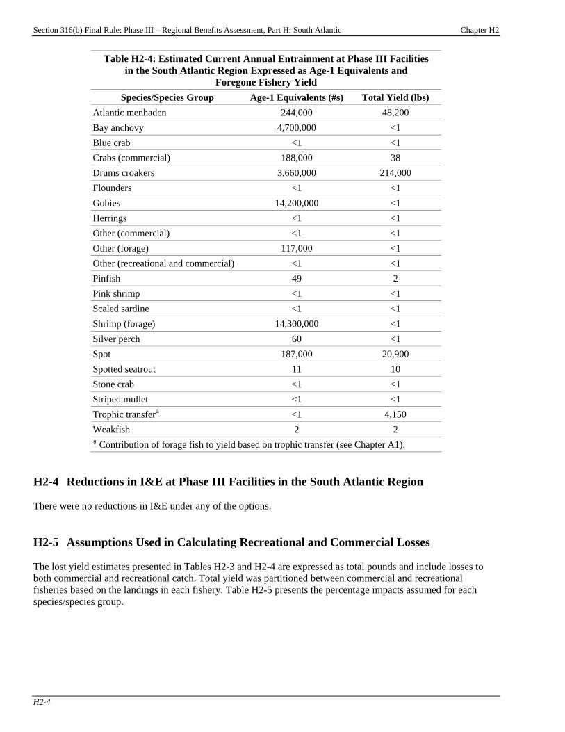
Section 316(b) Final Rule: Phase III – Regional Benefits Assessment, Part H: South Atlantic Chapter H2
H2-4
Table H2-4: Estimated Current Annual Entrainment at Phase III Facilities in the South Atlantic Region Expressed as Age-1 Equivalents and
Foregone Fishery Yield Species/Species Group Age-1 Equivalents (#s) Total Yield (lbs)
Atlantic menhaden 244,000 48,200 Bay anchovy 4,700,000 <1 Blue crab <1 <1 Crabs (commercial) 188,000 38 Drums croakers 3,660,000 214,000 Flounders <1 <1 Gobies 14,200,000 <1 Herrings <1 <1 Other (commercial) <1 <1 Other (forage) 117,000 <1 Other (recreational and commercial) <1 <1 Pinfish 49 2 Pink shrimp <1 <1 Scaled sardine <1 <1 Shrimp (forage) 14,300,000 <1 Silver perch 60 <1 Spot 187,000 20,900 Spotted seatrout 11 10 Stone crab <1 <1 Striped mullet <1 <1 Trophic transferP
aP <1 4,150
Weakfish 2 2 P
aP Contribution of forage fish to yield based on trophic transfer (see Chapter A1).
H2-4 Reductions in I&E at Phase III Facilities in the South Atlantic Region There were no reductions in I&E under any of the options. H2-5 Assumptions Used in Calculating Recreational and Commercial Losses The lost yield estimates presented in Tables H2-3 and H2-4 are expressed as total pounds and include losses to both commercial and recreational catch. Total yield was partitioned between commercial and recreational fisheries based on the landings in each fishery. Table H2-5 presents the percentage impacts assumed for each species/species group.
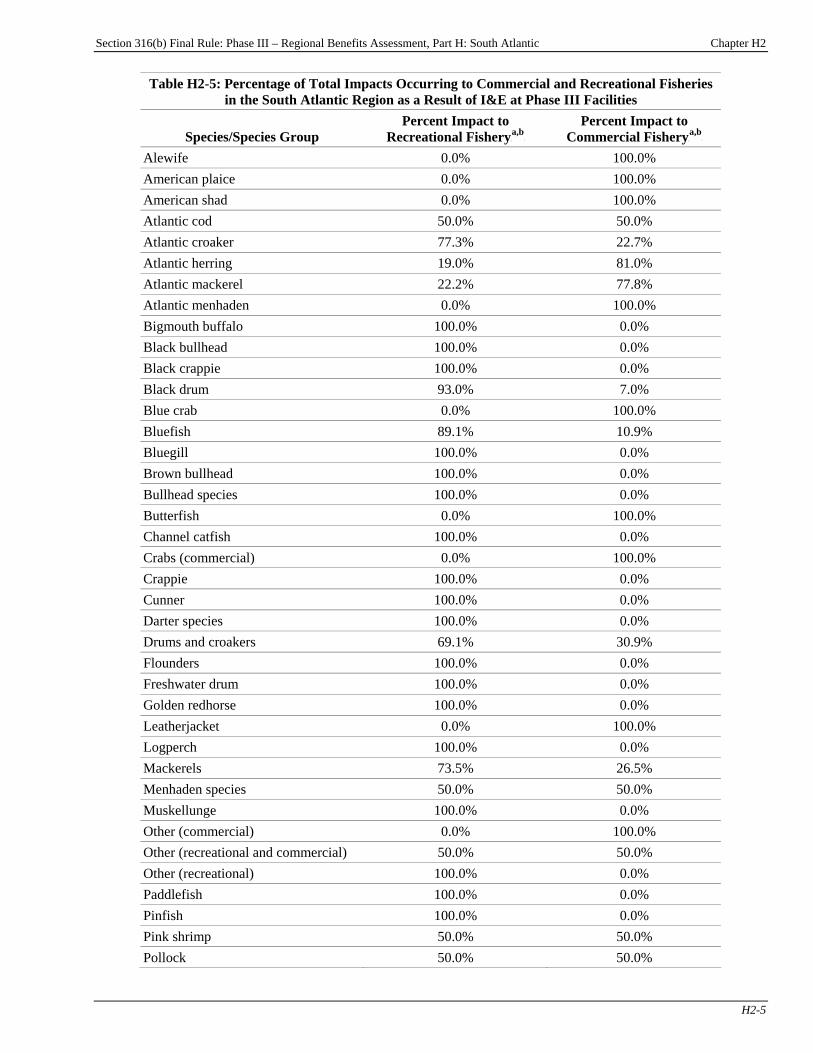
Section 316(b) Final Rule: Phase III – Regional Benefits Assessment, Part H: South Atlantic Chapter H2
H2-5
Table H2-5: Percentage of Total Impacts Occurring to Commercial and Recreational Fisheries in the South Atlantic Region as a Result of I&E at Phase III Facilities
Species/Species Group Percent Impact to
Recreational FisheryP
a,bP
Percent Impact to Commercial FisheryP
a,bP
Alewife 0.0% 100.0% American plaice 0.0% 100.0% American shad 0.0% 100.0% Atlantic cod 50.0% 50.0% Atlantic croaker 77.3% 22.7% Atlantic herring 19.0% 81.0% Atlantic mackerel 22.2% 77.8% Atlantic menhaden 0.0% 100.0% Bigmouth buffalo 100.0% 0.0% Black bullhead 100.0% 0.0% Black crappie 100.0% 0.0% Black drum 93.0% 7.0% Blue crab 0.0% 100.0% Bluefish 89.1% 10.9% Bluegill 100.0% 0.0% Brown bullhead 100.0% 0.0% Bullhead species 100.0% 0.0% Butterfish 0.0% 100.0% Channel catfish 100.0% 0.0% Crabs (commercial) 0.0% 100.0% Crappie 100.0% 0.0% Cunner 100.0% 0.0% Darter species 100.0% 0.0% Drums and croakers 69.1% 30.9% Flounders 100.0% 0.0% Freshwater drum 100.0% 0.0% Golden redhorse 100.0% 0.0% Leatherjacket 0.0% 100.0% Logperch 100.0% 0.0% Mackerels 73.5% 26.5% Menhaden species 50.0% 50.0% Muskellunge 100.0% 0.0% Other (commercial) 0.0% 100.0% Other (recreational and commercial) 50.0% 50.0% Other (recreational) 100.0% 0.0% Paddlefish 100.0% 0.0% Pinfish 100.0% 0.0% Pink shrimp 50.0% 50.0% Pollock 50.0% 50.0%
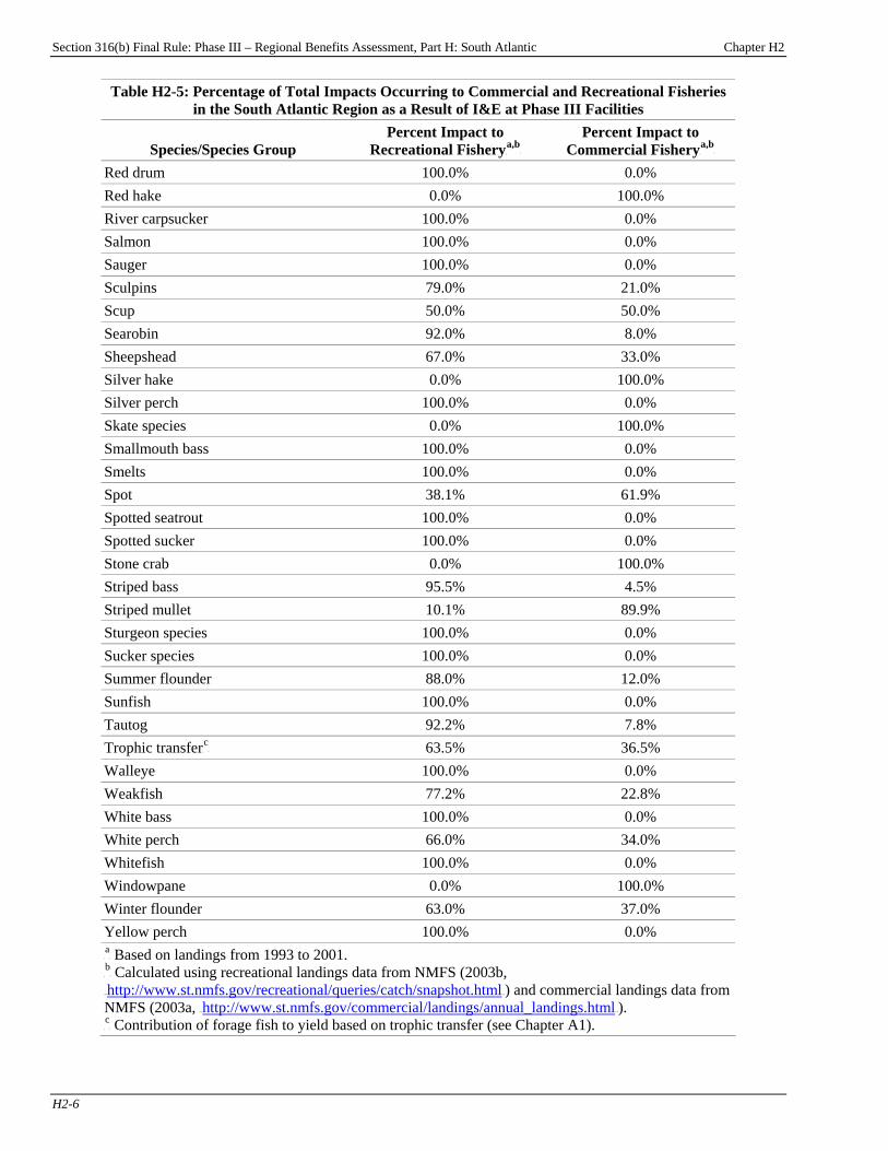
Section 316(b) Final Rule: Phase III – Regional Benefits Assessment, Part H: South Atlantic Chapter H2
H2-6
Table H2-5: Percentage of Total Impacts Occurring to Commercial and Recreational Fisheries in the South Atlantic Region as a Result of I&E at Phase III Facilities
Species/Species Group Percent Impact to
Recreational FisheryP
a,bP
Percent Impact to Commercial FisheryP
a,bP
Red drum 100.0% 0.0% Red hake 0.0% 100.0% River carpsucker 100.0% 0.0% Salmon 100.0% 0.0% Sauger 100.0% 0.0% Sculpins 79.0% 21.0% Scup 50.0% 50.0% Searobin 92.0% 8.0% Sheepshead 67.0% 33.0% Silver hake 0.0% 100.0% Silver perch 100.0% 0.0% Skate species 0.0% 100.0% Smallmouth bass 100.0% 0.0% Smelts 100.0% 0.0% Spot 38.1% 61.9% Spotted seatrout 100.0% 0.0% Spotted sucker 100.0% 0.0% Stone crab 0.0% 100.0% Striped bass 95.5% 4.5% Striped mullet 10.1% 89.9% Sturgeon species 100.0% 0.0% Sucker species 100.0% 0.0% Summer flounder 88.0% 12.0% Sunfish 100.0% 0.0% Tautog 92.2% 7.8% Trophic transferP
cP 63.5% 36.5%
Walleye 100.0% 0.0% Weakfish 77.2% 22.8% White bass 100.0% 0.0% White perch 66.0% 34.0% Whitefish 100.0% 0.0% Windowpane 0.0% 100.0% Winter flounder 63.0% 37.0% Yellow perch 100.0% 0.0% P
aP Based on landings from 1993 to 2001.
P
bP Calculated using recreational landings data from NMFS (2003b,
HTUhttp://www.st.nmfs.gov/recreational/queries/catch/snapshot.htmlUTH) and commercial landings data from NMFS (2003a, HTUhttp://www.st.nmfs.gov/commercial/landings/annual_landings.htmlUTH). P
cP Contribution of forage fish to yield based on trophic transfer (see Chapter A1).

Section 316(b) Final Rule: Phase III – Regional Benefits Assessment, Part H: South Atlantic Appendix H2
App. H2-1
Appendix H2: Reductions in I&E Under Supplemental Policy Options
Table H2-1: Estimated Reductions in I&E in the South Atlantic Region Under Supplemental Options
Option Age-1 Equivalents
(#s) Foregone Fishery Yield
(lbs) Electric Generators 2-50 MGD
I-only Everywhere 0 0 I&E like Phase II 0 0 I&E Everywhere 0 0
Manufacturers 2-50 MGD I-only Everywhere 0 0 I&E like Phase II 0 0 I&E Everywhere 0 0
Manufacturers 50+ MGD I-only Everywhere 0 0 I&E Everywhere 0 0
Section 316(b) Final Rule: Phase III – Regional Benefits Assessment, Part H: South Atlantic Chapter H3
H3-1
Chapter H3: Commercial Fishing Benefits Introduction This chapter presents the results of the commercial fishing benefits analysis for the South Atlantic region. The chapter presents EPA’s estimates of baseline (i.e., current) annual commercial fishery losses from impingement and entrainment (I&E) at potentially regulated facilities in the South Atlantic region and annual reductions in these losses under the regulatory options for Phase III existing facilitiesPF
1FP:
Chapter Contents H3-1 Baseline Commercial Losses ........................H3-1 H3-2 Expected Benefits Under Regulatory Analysis Options...........................................H3-2
< the “50 MGD for All Waterbodies” option, < the “200 MGD for All Waterbodies” option, and < the “100 MGD for Certain Waterbodies” option.
The chapter then presents the estimated benefits to commercial fisheries under the regulatory options from eliminating baseline losses from I&E. Chapter A4, “Methods for Estimating Commercial Fishing Benefits,” details the methods used by EPA to estimate the commercial fishing benefits of reducing and eliminating I&E losses. EPA considered a wide range of policy options in developing this regulation. In addition to the regulatory options, EPA evaluated supplemental options. For additional information on the options, please see the TDD. Appendix H3 presents results of the commercial fishing benefits analysis for the supplemental options. H3-1 Baseline Commercial Losses Table H3-1 provides EPA’s estimate of the value of gross revenues lost in commercial fisheries resulting from the impingement of aquatic species at facilities in the South Atlantic region. Table H3-2 displays this information for entrainment. Total annualized revenue losses are approximately $99,210 (undiscounted).
P
1P See the Introduction to this report for a description of the regulatory options.

Section 316(b) Final Rule: Phase III – Regional Benefits Assessment, Part H: South Atlantic Chapter H3
H3-2
Table H3-1: Annualized Commercial Fishing Gross Revenues Lost due to Impingement at Facilities in the South Atlantic Region
SpeciesP
aP
Estimated Pounds of
Harvest Lost
Commercial Value per
Pound (2004$)
Estimated Value of Harvest Lost
(2004$) Undiscounted
Atlantic menhaden 19,565 $0.07 $1,357 Blue crab 54 $0.74 $40 Drums and croakers 4,888 $1.06 $5,180 Other (species are only commercially fished not recreationally) 36 $0.56 $20
Other (species are fished both commercially and recreationally) 13 $0.56 $7
Pink shrimp 1 $1.24 $2 Spot 35,228 $0.37 $13,016 Stone crab 12 $1.54 $18 Striped Mullet 4 $0.71 $3 Weakfish 720 $0.69 $497 Trophic transferP
bP 180 $0.54 $97
P
aP Species included are only those that have baseline losses greater than $1.
P
bP Contribution of forage fish to yield based on trophic transfer (see Chapter A1).
Table H3-2: Annualized Commercial Fishing Gross Revenues Lost due to Entrainment at Facilities in the South Atlantic Region
SpeciesP
aP
Estimated Pounds of
Harvest Lost
Commercial Value per
Pound (2004$)
Estimated Value of Harvest Lost
(2004$) Undiscounted
Atlantic menhaden 48,231 $0.07 $3,344 Commercial crabs 38 $0.57 $21
Drums and croakers 66,058 $1.06 $70,009 Spot 12,947 $0.37 $4,784 Trophic. transferP
bP 1,516 $0.54 $815
P
aP Species included are only those that have baseline losses greater than $1.
P
bP Contribution of forage fish to yield based on trophic transfer (see Chapter
A1). H3-2 Expected Benefits Under Regulatory Analysis Options There are no facilities in the South Atlantic region that have technology requirements under any of the three regulatory options. Thus, no commercial fishing benefits are expected from the three regulatory options, the “50 MGD for All Waterbodies” option, the “200 MGD for All Waterbodies” option, and the “100 MGD for Certain Waterbodies” option, in the South Atlantic Region.

Section 316(b) Final Rule: Phase III – Regional Benefits Assessment, Part H: South Atlantic Appendix H3
App. H3-1
Appendix H3: Commercial Fishing Benefits Under Supplemental Policy Options
Introduction Chapter H3 presents EPA’s estimates of the commercial benefits of the three regulatory options for the section 316(b) rule for Phase III facilities in the South Atlantic region. To facilitate comparisons among the options, this appendix presents estimates of the commercial fishing benefits of various supplemental options that EPA evaluated in preparation for this rule:
Appendix Contents H3-1 Commercial Fishing Benefits of the
Supplemental Options ................................ H3-1
< “Electric Generators 2-50 MGD I-only Everywhere” option; < “Electric Generators 2-50 MGD I&E like Phase II” option; < “Electric Generators 2-50 MGD I&E Everywhere” option; < “Manufacturers 2-50 MGD I-only Everywhere” option; < “Manufacturers 2-50 MGD I&E like Phase II” option; < “Manufacturers 2-50 MGD I&E Everywhere” option; < “Manufacturers 50+ MGD I-only Everywhere” option; and < “Manufacturers 50+ MGD I&E Everywhere” option.
For additional information on the options, please see the TDD. Commercial fishing benefits presented in this chapter were estimated using the benefit transfer approach discussed in Chapter H3 and in Chapter A4, “Methods for Estimating Commercial Fishing Benefits.” H3-1 Commercial Fishing Benefits of the Supplemental Options No facilities located in the South Atlantic region have technology requirements under the supplemental options. Thus, no reductions in commercial fishing losses are expected under the supplemental options in the South Atlantic region.
Section 316(b) Final Rule: Phase III – Regional Benefits Assessment, Part H: South Atlantic Chapter H4
H4-1
Chapter H4: Recreational Use Benefits
Chapter Contents H4-1 Benefit Transfer Approach Based on Meta- Analysis ........................................................ H4-1 H4-1.1 Baseline Losses and Reductions in Recreational Fishery Losses Under the Regulatory Options ................... H4-2 H4-1.2 Recreational Fishing Benefits from Eliminating Baseline I&E Losses.............................................. H4-3 H4-1.3 Recreational Fishing Benefits of the “50 MGD for All Waterbodies” Option ............................................. H4-4 H4-1.4 Recreational Fishing Benefits of the “200 MGD for All Waterbodies” Option ............................................. H4-4 H4-1.5 Recreational Fishing Benefits of the “100 MGD for Certain Waterbodies” Option ............................................. H4-4 H4-2 Limitations and Uncertainty ......................... H4-4
Introduction This chapter presents the results of the recreational fishing benefits analysis for the South Atlantic region. The chapter presents EPA’s estimates of baseline (i.e., current) annual recreational fishery losses from impingement and entrainment (I&E) at potentially regulated facilities in the South Atlantic region and annual reductions in these losses under the regulatory options for Phase III existing facilitiesPF
1FP:
< the “50 MGD for All Waterbodies” option, < the “200 MGD for All Waterbodies” option,
and < the “100 MGD for Certain Waterbodies”
option. The chapter then presents the estimated welfare gain to South Atlantic anglers from eliminating baseline recreational fishing losses from I&E and the expected benefits under the regulatory options. EPA estimated the recreational benefits of reducing and eliminating I&E losses using a benefit transfer methodology based on a meta-analysis of the marginal value of catching different species of fish. This meta-analysis is discussed in detail in Chapter A5, “Recreational Fishing Benefits Methodology.” EPA considered a wide range of policy options in developing this regulation. In addition to the regulatory options, EPA evaluated supplemental options. For additional information on the options, please see the TDD. Appendix H4 presents results of the recreational fishing benefits analysis for the supplemental options. H4-1 Benefit Transfer Approach Based on Meta-Analysis EPA estimated the recreational welfare gain from the reduction in annual I&E losses expected under the policy options, and the welfare gain from eliminating I&E at potentially regulated facilities, using a benefit transfer approach. As discussed in Chapter A5, the Agency used a meta-analysis regression equation to estimate the marginal recreational value per additional fish caught by anglers, for different species in different regions. Since I&E at potentially regulated facilities affects a variety of species, EPA assigned each species with I&E losses to one of the general species groups used in the meta-analysis. The Agency then calculated the economic value of reducing or eliminating baseline I&E losses, for each species group, by multiplying the value per fish for that species group by the number of fish in the group that are lost in the baseline or saved under the policy options.PF
2FP
P
1P See the Introduction to this report for a description of the regulatory options.
P
2P The estimates of I&E presented in this chapter include only the fraction of impinged and entrained recreational
fish that would be caught by anglers. The total amount of I&E of recreational species is actually much higher.

Section 316(b) Final Rule: Phase III – Regional Benefits Assessment, Part H: South Atlantic Chapter H4
H4-2
In general, the fit between the species with I&E losses and the species groups in the meta-analysis was good. However, EPA’s estimates of baseline I&E losses and reductions in I&E under the policy options included losses of “unidentified” species. The “unidentified” group includes fish lost indirectly through trophic transfer, as well as species for which no species information was available.PF
3FP Rather than using the meta-analysis regression to try to
predict the value per fish for an “unidentified” species, EPA assumed that per-fish values for these species can be approximated by the weighted average value per fish for all species affected by I&E in the South Atlantic region.PF
4FP
H4-1.1 Baseline Losses and Reductions in Recreational Fishery Losses Under the Regulatory Options Table H4-1 presents EPA’s estimates of baseline (i.e., current) annual recreational I&E losses at potentially regulated facilities, and annual reductions in these losses under each of the regulatory options, in the South Atlantic region. The table shows that total baseline losses to recreational fisheries are 549.2 thousand fish per year. In comparison, the “50 MGD for All Waterbodies” option prevents losses of 0 fish per year, the “200 MGD for All Waterbodies” option prevents losses of 0 fish per year, and the “100 MGD for Certain Waterbodies” option prevents losses of 0 fish per year. Of all the affected species, croakers and spot have the highest losses in the baseline.
P
3P In addition to recreational fish that are lost because they are impinged or entrained, some recreational fish are lost
because the forage fish that they feed on are impinged or entrained, and thus removed from the food chain. These trophic transfer losses of recreational species are included in EPA’s estimates of total I&E losses. Since it is difficult to predict which recreational species would be affected by losses of forage fish, these losses are classified as “unidentified” recreational species. Also included in the “unidentified” group are losses of fish that were reported by facilities without information about their exact species.
P
4P EPA used the estimated level of baseline recreational losses for each species group as a weighting factor.
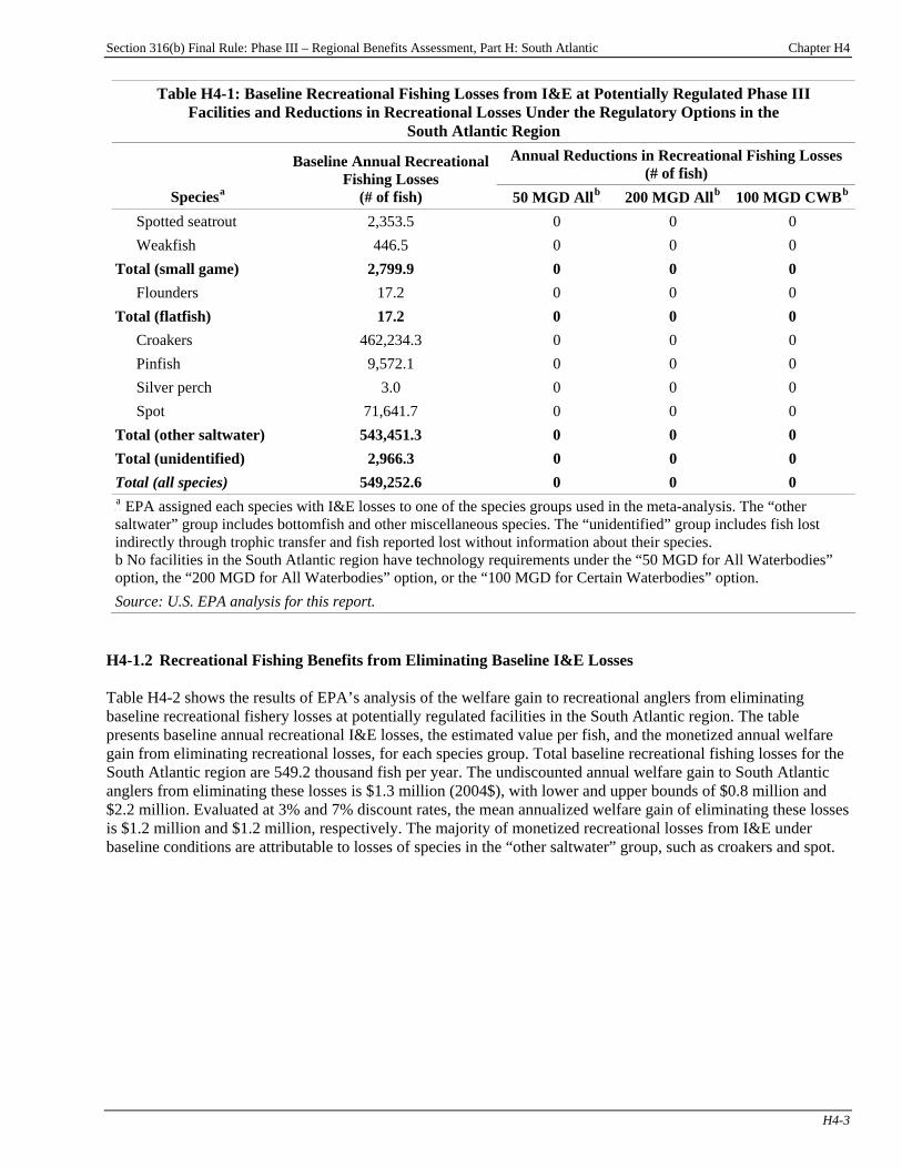
Section 316(b) Final Rule: Phase III – Regional Benefits Assessment, Part H: South Atlantic Chapter H4
H4-3
Table H4-1: Baseline Recreational Fishing Losses from I&E at Potentially Regulated Phase III Facilities and Reductions in Recreational Losses Under the Regulatory Options in the
South Atlantic Region Annual Reductions in Recreational Fishing Losses
(# of fish) SpeciesP
aP
Baseline Annual Recreational Fishing Losses
(# of fish) 50 MGD AllP
bP 200 MGD AllP
bP 100 MGD CWBP
bP
Spotted seatrout 2,353.5 0 0 0 Weakfish 446.5 0 0 0
Total (small game) 2,799.9 0 0 0 Flounders 17.2 0 0 0
Total (flatfish) 17.2 0 0 0 Croakers 462,234.3 0 0 0 Pinfish 9,572.1 0 0 0 Silver perch 3.0 0 0 0 Spot 71,641.7 0 0 0
Total (other saltwater) 543,451.3 0 0 0 Total (unidentified) 2,966.3 0 0 0 Total (all species) 549,252.6 0 0 0 P
aP EPA assigned each species with I&E losses to one of the species groups used in the meta-analysis. The “other
saltwater” group includes bottomfish and other miscellaneous species. The “unidentified” group includes fish lost indirectly through trophic transfer and fish reported lost without information about their species. b No facilities in the South Atlantic region have technology requirements under the “50 MGD for All Waterbodies” option, the “200 MGD for All Waterbodies” option, or the “100 MGD for Certain Waterbodies” option. Source: U.S. EPA analysis for this report.
H4-1.2 Recreational Fishing Benefits from Eliminating Baseline I&E Losses Table H4-2 shows the results of EPA’s analysis of the welfare gain to recreational anglers from eliminating baseline recreational fishery losses at potentially regulated facilities in the South Atlantic region. The table presents baseline annual recreational I&E losses, the estimated value per fish, and the monetized annual welfare gain from eliminating recreational losses, for each species group. Total baseline recreational fishing losses for the South Atlantic region are 549.2 thousand fish per year. The undiscounted annual welfare gain to South Atlantic anglers from eliminating these losses is $1.3 million (2004$), with lower and upper bounds of $0.8 million and $2.2 million. Evaluated at 3% and 7% discount rates, the mean annualized welfare gain of eliminating these losses is $1.2 million and $1.2 million, respectively. The majority of monetized recreational losses from I&E under baseline conditions are attributable to losses of species in the “other saltwater” group, such as croakers and spot.
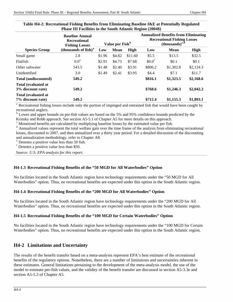
Section 316(b) Final Rule: Phase III – Regional Benefits Assessment, Part H: South Atlantic Chapter H4
H4-4
Table H4-2: Recreational Fishing Benefits from Eliminating Baseline I&E at Potentially Regulated Phase III Facilities in the South Atlantic Region (2004$)
Value per FishP
bP
Annualized Benefits from Eliminating Recreational Fishing Losses
(thousands)P
c,dP
Species Group
Baseline Annual Recreational
Fishing Losses (thousands of fish)P
aP Low Mean High Low Mean High
Small game 2.8 $1.96 $4.82 $11.60 $5.5 $13.5 $32.5 Flatfish 0.0P
eP $2.91 $4.73 $7.68 $0.0P
fP $0.1 $0.1
Other saltwater 543.5 $1.48 $2.40 $3.91 $806.2 $1,302.8 $2,124.3 Unidentified 3.0 $1.49 $2.41 $3.95 $4.4 $7.1 $11.7 Total (undiscounted) 549.2 $816.1 $1,323.5 $2,168.6 Total (evaluated at 3% discount rate) 549.2 $768.6 $1,246.3 $2,042.2 Total (evaluated at 7% discount rate) 549.2 $712.4 $1,155.3 $1,893.1 P
aP Recreational fishing losses include only the portion of impinged and entrained fish that would have been caught by
recreational anglers. P
bP Lower and upper bounds on per-fish values are based on the 5% and 95% confidence bounds predicted by the
Krinsky and Robb approach. See section A5-5.1 of Chapter A5 for more details on this approach. P
cP Monetized benefits are calculated by multiplying baseline losses by the estimated value per fish.
P
dP Annualized values represent the total welfare gain over the time frame of the analysis from eliminating recreational
losses, discounted to 2007, and then annualized over a thirty year period. For a detailed discussion of the discounting and annualization methodology, refer to Chapter A8. P
eP Denotes a positive value less than 50 fish.
P
fP Denotes a positive value less than $50.
Source: U.S. EPA analysis for this report. H4-1.3 Recreational Fishing Benefits of the “50 MGD for All Waterbodies” Option No facilities located in the South Atlantic region have technology requirements under the “50 MGD for All Waterbodies” option. Thus, no recreational benefits are expected under this option in the South Atlantic region. H4-1.4 Recreational Fishing Benefits of the “200 MGD for All Waterbodies” Option No facilities located in the South Atlantic region have technology requirements under the “200 MGD for All Waterbodies” option. Thus, no recreational benefits are expected under this option in the South Atlantic region. H4-1.5 Recreational Fishing Benefits of the “100 MGD for Certain Waterbodies” Option No facilities located in the South Atlantic region have technology requirements under the “100 MGD for Certain Waterbodies” option. Thus, no recreational benefits are expected under this option in the South Atlantic region. H4-2 Limitations and Uncertainty The results of the benefit transfer based on a meta-analysis represent EPA’s best estimate of the recreational benefits of the regulatory options. Nonetheless, there are a number of limitations and uncertainties inherent in these estimates. General limitations pertaining to the development of the meta-analysis model, the use of the model to estimate per-fish values, and the validity of the benefit transfer are discussed in section A5-3.3e and section A5-5.3 of Chapter A5.
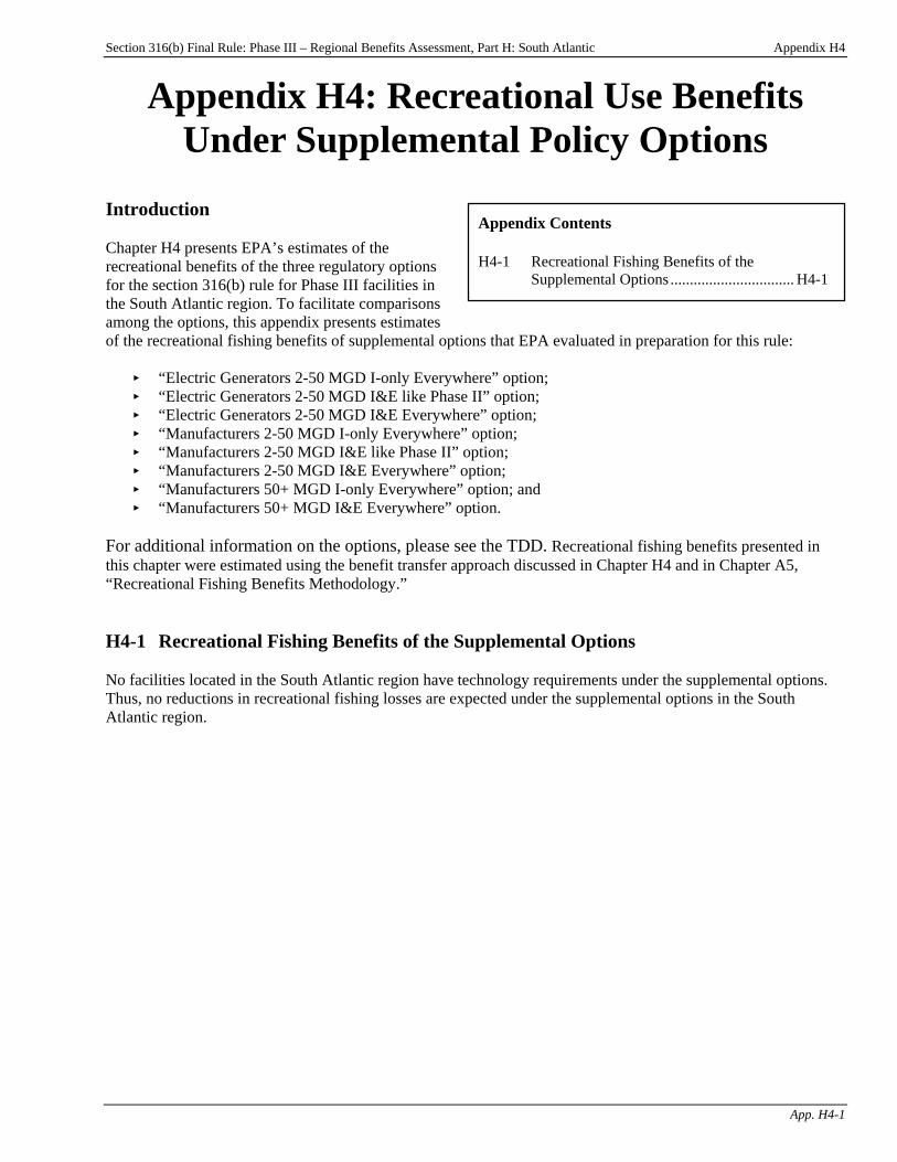
Section 316(b) Final Rule: Phase III – Regional Benefits Assessment, Part H: South Atlantic Appendix H4
App. H4-1
Appendix H4: Recreational Use Benefits Under Supplemental Policy Options
Introduction Chapter H4 presents EPA’s estimates of the recreational benefits of the three regulatory options for the section 316(b) rule for Phase III facilities in the South Atlantic region. To facilitate comparisons among the options, this appendix presents estimates of the recreational fishing benefits of supplemental options that EPA evaluated in preparation for this rule:
Appendix Contents H4-1 Recreational Fishing Benefits of the
Supplemental Options ................................ H4-1
< “Electric Generators 2-50 MGD I-only Everywhere” option; < “Electric Generators 2-50 MGD I&E like Phase II” option; < “Electric Generators 2-50 MGD I&E Everywhere” option; < “Manufacturers 2-50 MGD I-only Everywhere” option; < “Manufacturers 2-50 MGD I&E like Phase II” option; < “Manufacturers 2-50 MGD I&E Everywhere” option; < “Manufacturers 50+ MGD I-only Everywhere” option; and < “Manufacturers 50+ MGD I&E Everywhere” option.
For additional information on the options, please see the TDD. Recreational fishing benefits presented in this chapter were estimated using the benefit transfer approach discussed in Chapter H4 and in Chapter A5, “Recreational Fishing Benefits Methodology.” H4-1 Recreational Fishing Benefits of the Supplemental Options No facilities located in the South Atlantic region have technology requirements under the supplemental options. Thus, no reductions in recreational fishing losses are expected under the supplemental options in the South Atlantic region.

Section 316(b) Final Rule: Phase III – Regional Benefits Assessment, Part H: South Atlantic Chapter H5
H5-1
Chapter H5: Federally Listed T&E Species in the South Atlantic Region
This chapter lists current federally listed threatened and endangered (T&E) fish and shellfish species in the South Atlantic Region. This list does not address proposed or candidate species; In addition, fish and shellfish listed as cave species, marine mammals, reptiles, amphibians, and snails are not included in this chapter.
Table H5-1: Florida Federally Listed T&E Fish and Shellfish Status Scientific Name Common Name
E Acipenser brevirostrum Shortnose sturgeon T Acipenser oxyrinchus desotoi Gulf sturgeon E Amblema neislerii Fat three-ridge mussel T Elliptio chipolaensis Chipola slabshell mussel T Elliptoideus sloatianus Purple bankclimber mussel E Etheostoma okaloosae Okaloosa darter E Lampsilis subangulata Shinyrayed pocketbook mussel E Medionidus penicillatus Gulf moccasinshell E Medionidus simpsonianus Ochlockonee moccasinshell E Pleurobema pyriforme Oval pigtoe mussel E Pristis pectinata Smalltooth sawfish
Source: USFWS, 2006a.
Table H5-2: Georgia Federally Listed T&E Fish and Shellfish Status Scientific Name Common Name
T Elliptoideus sloatianus Purple bankclimber mussel T Medionidus acutissimus Alabama moccasinshell E Pleurobema decisum Southern clubshell mussel E Acipenser brevirostrum Shortnose sturgeon T Acipenser oxyrinchus desotoi Gulf sturgeon E Amblema neislerii Fat three-ridge mussel T Cyprinella caerulea Blue shiner E Epioblasma capsaeformis Oyster mussel: entire range except where listed as
experimental populations E Epioblasma metastriata Upland combshell mussel E Epioblasma othcaloogensis Southern acornshell mussel T Erimonax monachus Spotfin chub: entire range except where listed as
experimental populations E Etheostoma etowahae Etowah darter T Etheostoma scotti Cherokee darter T Lampsilis altilis Finelined pocketbook mussel E Lampsilis subangulata Shinyrayed pocketbook mussel

Section 316(b) Final Rule: Phase III – Regional Benefits Assessment, Part H: South Atlantic Chapter H5
H5-2
Table H5-2: Georgia Federally Listed T&E Fish and Shellfish Status Scientific Name Common Name
E Medionidus parvulus Coosa moccasinshell E Medionidus penicillatus Gulf moccasinshell E Medionidus simpsonianus Ochlockonee moccasinshell E Percina antesella Amber darter T Percina aurolineata Goldline darter E Percina jenkinsi Conasauga logperch T Percina tanasi Snail darter E Pleurobema georgianum Southern pigtoe mussel E Pleurobema perovatum Ovate clubshell mussel E Pleurobema pyriforme Oval pigtoe mussel E Ptychobranchus greenii Triangular kidneyshell mussel
Source: USFWS, 2006a.
Table H5-3: North Carolina Federally Listed T&E Fish and Shellfish Status Scientific Name Common Name
E Acipenser brevirostrum Shortnose sturgeon E Alasmidonta raveneliana Appalachian elktoe mussel E Elliptio steinstansana Tar River spinymussel E Epioblasma capsaeformis Oyster mussel: entire range except where listed as
experimental populations E Epioblasma florentina walkeri ( = E. walkeri) Tan riffleshell mussel T Erimonax monachus Spotfin chub: entire range except where listed as
experimental populations E Lasmigona decorata Carolina heelsplitter mussel T Menidia extensa Waccamaw silverside E Notropis mekistocholas Cape Fear shiner E Pegias fabula Littlewing pearlymussel E Pristis pectinata Smalltooth sawfish
Source: USFWS, 2006a.
Table H5-4: South Carolina Federally Listed T&E Fish and Shellfish Status Scientific Name Common Name
E Acipenser brevirostrum Shortnose sturgeon E Lasmigona decorata Carolina heelsplitter mussel E Pristis pectinata Smalltooth sawfish
Source: USFWS, 2006a.

Section 316(b) Final Rule: Phase III – Regional Benefits Assessment
Part I: National Benefits

Section 316(b) Final Rule: Phase III – Regional Benefits Assessment, Part I: National Benefits Chapter I1
I1-1
Chapter I1: National Benefits Introduction
Chapter Contents I1-1 Calculating National Losses and Benefits.........I1-1 I1-2 Summary of Baseline Losses and Expected
Reductions in I&E.............................................I1-2 I1-3 Time Profile of Benefits....................................I1-4 I1-4 National Benefits from Eliminating and
Reducing I&E Losses......................................I1-12
This chapter summarizes the results of the seven regional analyses and presents EPA’s estimates of the national commercial and recreational benefits of the regulatory analysis options for Phase III existing facilities:
< the “50 MGD for All Waterbodies” option,
< the “200 MGD for All Waterbodies” option, and < the “100 MGD for Certain Waterbodies” option.
EPA considered a wide range of policy options in developing this regulation. Results of the national benefits analysis for supplemental options evaluated by EPA are presented in Appendix I1. Greater detail on the methods and data used in the regional analyses is provided in the previous chapters of this report. See Chapters A1 and A2 for a discussion of the methods used to estimate impingement and entrainment (I&E), and Chapters A3 through A9 for a discussion of the methods used to estimate the value of I&E losses and the benefits of the policy options considered for the final rule. The results of the regional analyses are presented in Parts B through H. EPA was unable to assess benefits of reducing I&E at existing offshore oil and gas extraction facilities in the same manner as other existing facilities, which would require predicting where these facilities would build and/or operate, and due to lack of I&E data for these facilities. Therefore, the benefits estimates presented in this section do not reflect benefits associated with reducing I&E at existing offshore oil and gas extraction facilities and overall national benefits may be accordingly higher. I1-1 Calculating National Losses and Benefits EPA’s analysis of national baseline losses and benefits under the regulatory analysis options includes 629 sample-weighted facilities, excluding facilities that are expected to close in the baseline. The Agency calculated baseline losses by summing losses from all 629 facilities in the seven case study regions. EPA’s estimates of benefits are based on only those facilities that would be expected to install compliance technologies under each regulatory analysis option because the baseline is best professional judgment. EPA notes that quantifying and monetizing reductions in I&E under the regulatory analysis options considered for the final section 316(b) rule for Phase III facilities is extremely challenging. As described in Chapters A3 and A6, EPA has estimated non-use values qualitatively and, as a result, the estimated monetized benefits of the regulatory analysis options reflect use values only. The preceding sections of this report discuss specific limitations and uncertainties associated with estimating commercial and recreational benefits. National benefit estimates, which are based on the regional estimates, are subject to the same uncertainties inherent in the valuation approaches used for assessing each of the two benefits categories. The combined effect of these uncertainties is of unknown magnitude and direction (i.e., the estimates may over- or understate the anticipated national level of use benefits). Nevertheless, EPA has no data to indicate that the results for any of the benefit categories are atypical or unreasonable.
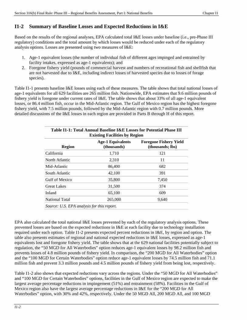
Section 316(b) Final Rule: Phase III – Regional Benefits Assessment, Part I: National Benefits Chapter I1
I1-2
I1-2 Summary of Baseline Losses and Expected Reductions in I&E Based on the results of the regional analyses, EPA calculated total I&E losses under baseline (i.e., pre-Phase III regulatory) conditions and the total amount by which losses would be reduced under each of the regulatory analysis options. Losses are presented using two measures of I&E:
1. Age-1 equivalent losses (the number of individual fish of different ages impinged and entrained by facility intakes, expressed as age-1 equivalents); and
2. Foregone fishery yield (pounds of commercial harvest and numbers of recreational fish and shellfish that are not harvested due to I&E, including indirect losses of harvested species due to losses of forage species).
Table I1-1 presents baseline I&E losses using each of these measures. The table shows that total national losses of age-1 equivalents for all 629 facilities are 265 million fish. Nationwide, EPA estimates that 9.6 million pounds of fishery yield is foregone under current rates of I&E. The table shows that about 33% of all age-1 equivalent losses, or 86.4 million fish, occur in the Mid-Atlantic region. The Gulf of Mexico region has the highest foregone fishery yield, with 7.5 million pounds, followed by the Mid-Atlantic region with 0.7 million pounds. More detailed discussions of the I&E losses in each region are provided in Parts B through H of this report.
Table I1-1: Total Annual Baseline I&E Losses for Potential Phase III Existing Facilities by Region
Region Age-1 Equivalents
(thousands) Foregone Fishery Yield
(thousands; lbs) California 1,710 121 North Atlantic 2,310 11 Mid-Atlantic 86,400 682 South Atlantic 42,100 391 Gulf of Mexico 35,800 7,450 Great Lakes 31,500 374 Inland 65,100 609 National Total 265,000 9,640 Source: U.S. EPA analysis for this report.
EPA also calculated the total national I&E losses prevented by each of the regulatory analysis options. These prevented losses are based on the expected reductions in I&E at each facility due to technology installation required under each option. Table I1-2 presents expected percent reductions in I&E, by region and option. The table also presents estimates of regional and national expected reductions in I&E losses, expressed as age-1 equivalents lost and foregone fishery yield. The table shows that at the 629 national facilities potentially subject to regulation, the “50 MGD for All Waterbodies” option reduces age-1 equivalent losses by 98.2 million fish and prevents losses of 4.8 million pounds of fishery yield. In comparison, the “200 MGD for All Waterbodies” option and the “100 MGD for Certain Waterbodies” option reduce age-1 equivalent losses by 74.5 million fish and 71.1 million fish and prevent 3.3 million pounds and 4.5 million pounds of fishery yield from being lost, respectively. Table I1-2 also shows that expected reductions vary across the regions. Under the “50 MGD for All Waterbodies” and “100 MGD for Certain Waterbodies” options, facilities in the Gulf of Mexico region are expected to make the largest average percentage reductions in impingement (51%) and entrainment (58%). Facilities in the Gulf of Mexico region also have the largest average percentage reductions in I&E for the “200 MGD for All Waterbodies” option, with 30% and 42%, respectively. Under the 50 MGD All, 200 MGD All, and 100 MGD
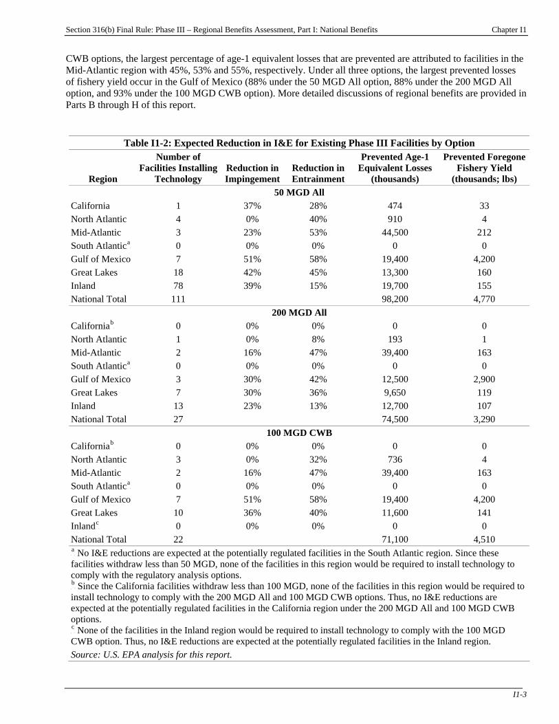
Section 316(b) Final Rule: Phase III – Regional Benefits Assessment, Part I: National Benefits Chapter I1
I1-3
CWB options, the largest percentage of age-1 equivalent losses that are prevented are attributed to facilities in the Mid-Atlantic region with 45%, 53% and 55%, respectively. Under all three options, the largest prevented losses of fishery yield occur in the Gulf of Mexico (88% under the 50 MGD All option, 88% under the 200 MGD All option, and 93% under the 100 MGD CWB option). More detailed discussions of regional benefits are provided in Parts B through H of this report.
Table I1-2: Expected Reduction in I&E for Existing Phase III Facilities by Option
Region
Number of Facilities Installing
Technology Reduction in Impingement
Reduction in Entrainment
Prevented Age-1 Equivalent Losses
(thousands)
Prevented Foregone Fishery Yield
(thousands; lbs) 50 MGD All
California 1 37% 28% 474 33 North Atlantic 4 0% 40% 910 4 Mid-Atlantic 3 23% 53% 44,500 212 South AtlanticP
aP 0 0% 0% 0 0
Gulf of Mexico 7 51% 58% 19,400 4,200 Great Lakes 18 42% 45% 13,300 160 Inland 78 39% 15% 19,700 155 National Total 111 98,200 4,770
200 MGD All CaliforniaP
bP 0 0% 0% 0 0
North Atlantic 1 0% 8% 193 1 Mid-Atlantic 2 16% 47% 39,400 163 South AtlanticP
aP 0 0% 0% 0 0
Gulf of Mexico 3 30% 42% 12,500 2,900 Great Lakes 7 30% 36% 9,650 119 Inland 13 23% 13% 12,700 107 National Total 27 74,500 3,290
100 MGD CWB CaliforniaP
bP 0 0% 0% 0 0
North Atlantic 3 0% 32% 736 4 Mid-Atlantic 2 16% 47% 39,400 163 South AtlanticP
aP 0 0% 0% 0 0
Gulf of Mexico 7 51% 58% 19,400 4,200 Great Lakes 10 36% 40% 11,600 141 InlandP
cP 0 0% 0% 0 0
National Total 22 71,100 4,510 P
aP No I&E reductions are expected at the potentially regulated facilities in the South Atlantic region. Since these
facilities withdraw less than 50 MGD, none of the facilities in this region would be required to install technology to comply with the regulatory analysis options. P
bP Since the California facilities withdraw less than 100 MGD, none of the facilities in this region would be required to
install technology to comply with the 200 MGD All and 100 MGD CWB options. Thus, no I&E reductions are expected at the potentially regulated facilities in the California region under the 200 MGD All and 100 MGD CWB options. P
cP None of the facilities in the Inland region would be required to install technology to comply with the 100 MGD
CWB option. Thus, no I&E reductions are expected at the potentially regulated facilities in the Inland region. Source: U.S. EPA analysis for this report.
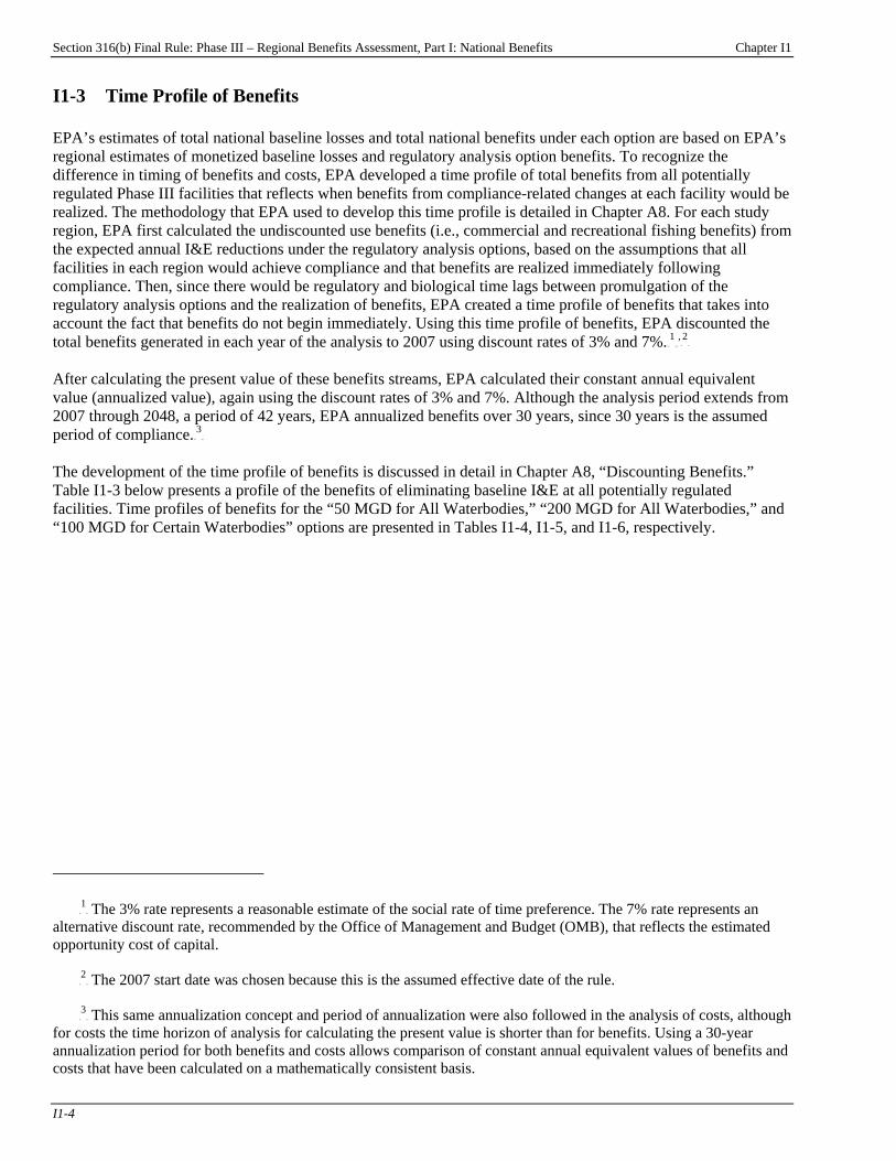
Section 316(b) Final Rule: Phase III – Regional Benefits Assessment, Part I: National Benefits Chapter I1
I1-4
I1-3 Time Profile of Benefits EPA’s estimates of total national baseline losses and total national benefits under each option are based on EPA’s regional estimates of monetized baseline losses and regulatory analysis option benefits. To recognize the difference in timing of benefits and costs, EPA developed a time profile of total benefits from all potentially regulated Phase III facilities that reflects when benefits from compliance-related changes at each facility would be realized. The methodology that EPA used to develop this time profile is detailed in Chapter A8. For each study region, EPA first calculated the undiscounted use benefits (i.e., commercial and recreational fishing benefits) from the expected annual I&E reductions under the regulatory analysis options, based on the assumptions that all facilities in each region would achieve compliance and that benefits are realized immediately following compliance. Then, since there would be regulatory and biological time lags between promulgation of the regulatory analysis options and the realization of benefits, EPA created a time profile of benefits that takes into account the fact that benefits do not begin immediately. Using this time profile of benefits, EPA discounted the total benefits generated in each year of the analysis to 2007 using discount rates of 3% and 7%.TPF
1FPTP
,TF
2FT
After calculating the present value of these benefits streams, EPA calculated their constant annual equivalent value (annualized value), again using the discount rates of 3% and 7%. Although the analysis period extends from 2007 through 2048, a period of 42 years, EPA annualized benefits over 30 years, since 30 years is the assumed period of compliance.TPF
3FPT
The development of the time profile of benefits is discussed in detail in Chapter A8, “Discounting Benefits.” Table I1-3 below presents a profile of the benefits of eliminating baseline I&E at all potentially regulated facilities. Time profiles of benefits for the “50 MGD for All Waterbodies,” “200 MGD for All Waterbodies,” and “100 MGD for Certain Waterbodies” options are presented in Tables I1-4, I1-5, and I1-6, respectively.
TP
1PT The 3% rate represents a reasonable estimate of the social rate of time preference. The 7% rate represents an
alternative discount rate, recommended by the Office of Management and Budget (OMB), that reflects the estimated opportunity cost of capital.
TP
2PT The 2007 start date was chosen because this is the assumed effective date of the rule.
TP
3PT This same annualization concept and period of annualization were also followed in the analysis of costs, although
for costs the time horizon of analysis for calculating the present value is shorter than for benefits. Using a 30-year annualization period for both benefits and costs allows comparison of constant annual equivalent values of benefits and costs that have been calculated on a mathematically consistent basis.
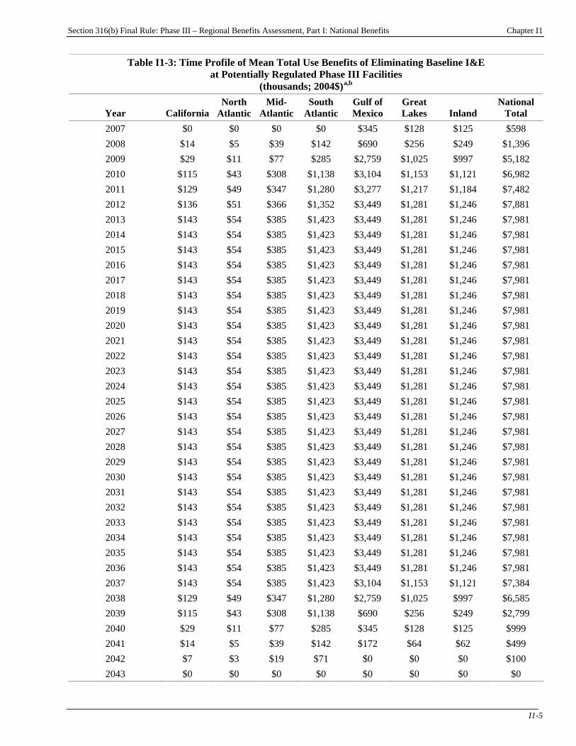
Section 316(b) Final Rule: Phase III – Regional Benefits Assessment, Part I: National Benefits Chapter I1
I1-5
Table I1-3: Time Profile of Mean Total Use Benefits of Eliminating Baseline I&E at Potentially Regulated Phase III Facilities
(thousands; 2004$)P
a,bP
Year California North
AtlanticMid-
AtlanticSouth
Atlantic Gulf of Mexico
Great Lakes Inland
National Total
2007 $0 $0 $0 $0 $345 $128 $125 $598 2008 $14 $5 $39 $142 $690 $256 $249 $1,396 2009 $29 $11 $77 $285 $2,759 $1,025 $997 $5,182 2010 $115 $43 $308 $1,138 $3,104 $1,153 $1,121 $6,982 2011 $129 $49 $347 $1,280 $3,277 $1,217 $1,184 $7,482 2012 $136 $51 $366 $1,352 $3,449 $1,281 $1,246 $7,881 2013 $143 $54 $385 $1,423 $3,449 $1,281 $1,246 $7,981 2014 $143 $54 $385 $1,423 $3,449 $1,281 $1,246 $7,981 2015 $143 $54 $385 $1,423 $3,449 $1,281 $1,246 $7,981 2016 $143 $54 $385 $1,423 $3,449 $1,281 $1,246 $7,981 2017 $143 $54 $385 $1,423 $3,449 $1,281 $1,246 $7,981 2018 $143 $54 $385 $1,423 $3,449 $1,281 $1,246 $7,981 2019 $143 $54 $385 $1,423 $3,449 $1,281 $1,246 $7,981 2020 $143 $54 $385 $1,423 $3,449 $1,281 $1,246 $7,981 2021 $143 $54 $385 $1,423 $3,449 $1,281 $1,246 $7,981 2022 $143 $54 $385 $1,423 $3,449 $1,281 $1,246 $7,981 2023 $143 $54 $385 $1,423 $3,449 $1,281 $1,246 $7,981 2024 $143 $54 $385 $1,423 $3,449 $1,281 $1,246 $7,981 2025 $143 $54 $385 $1,423 $3,449 $1,281 $1,246 $7,981 2026 $143 $54 $385 $1,423 $3,449 $1,281 $1,246 $7,981 2027 $143 $54 $385 $1,423 $3,449 $1,281 $1,246 $7,981 2028 $143 $54 $385 $1,423 $3,449 $1,281 $1,246 $7,981 2029 $143 $54 $385 $1,423 $3,449 $1,281 $1,246 $7,981 2030 $143 $54 $385 $1,423 $3,449 $1,281 $1,246 $7,981 2031 $143 $54 $385 $1,423 $3,449 $1,281 $1,246 $7,981 2032 $143 $54 $385 $1,423 $3,449 $1,281 $1,246 $7,981 2033 $143 $54 $385 $1,423 $3,449 $1,281 $1,246 $7,981 2034 $143 $54 $385 $1,423 $3,449 $1,281 $1,246 $7,981 2035 $143 $54 $385 $1,423 $3,449 $1,281 $1,246 $7,981 2036 $143 $54 $385 $1,423 $3,449 $1,281 $1,246 $7,981 2037 $143 $54 $385 $1,423 $3,104 $1,153 $1,121 $7,384 2038 $129 $49 $347 $1,280 $2,759 $1,025 $997 $6,585 2039 $115 $43 $308 $1,138 $690 $256 $249 $2,799 2040 $29 $11 $77 $285 $345 $128 $125 $999 2041 $14 $5 $39 $142 $172 $64 $62 $499 2042 $7 $3 $19 $71 $0 $0 $0 $100 2043 $0 $0 $0 $0 $0 $0 $0 $0

Section 316(b) Final Rule: Phase III – Regional Benefits Assessment, Part I: National Benefits Chapter I1
I1-6
Table I1-3: Time Profile of Mean Total Use Benefits of Eliminating Baseline I&E at Potentially Regulated Phase III Facilities
(thousands; 2004$)P
a,bP
Year California North
Atlantic Mid-
AtlanticSouth
Atlantic Gulf of Mexico
Great Lakes Inland
National Total
2044 $0 $0 $0 $0 $0 $0 $0 $0 2045 $0 $0 $0 $0 $0 $0 $0 $0 2046 $0 $0 $0 $0 $0 $0 $0 $0 2047 $0 $0 $0 $0 $0 $0 $0 $0 2048 $0 $0 $0 $0 $0 $0 $0 $0
Evaluated at 0% (i.e., undiscounted) Present valueP
cP $4,300 $1,624 $11,554 $42,681 $103,476 $38,424 $37,375 $239,434
Annualized valueP
dP $143 $54 $385 $1,423 $3,449 $1,281 $1,246 $7,981
Evaluated at 3% Discount Rate Present valueP
cP $2,646 $999 $7,109 $26,260 $65,575 $24,350 $23,685 $150,625
Annualized valueP
dP $135 $51 $363 $1,340 $3,346 $1,242 $1,208 $7,685
Evaluated at 7% Discount Rate Present valueP
cP $1,553 $586 $4,172 $15,411 $39,979 $14,845 $14,440 $90,986
Annualized valueP
dP $125 $47 $336 $1,242 $3,222 $1,196 $1,164 $7,332
P
aP This table presents the benefits of eliminating baseline I&E at potentially regulated Phase III facilities from 2007 to
2036. P
bP Because EPA estimated non-use benefits qualitatively, the monetary value of benefits includes only use values.
P
cP Values for a given year in the table are not discounted. Total present values of benefits are discounted with the
corresponding rate. P
dP Annualized benefits represent the value of all benefits generated over the time frame of the analysis, discounted to
2007, and then annualized over a thirty year period. Source: U.S. EPA analysis for this report.
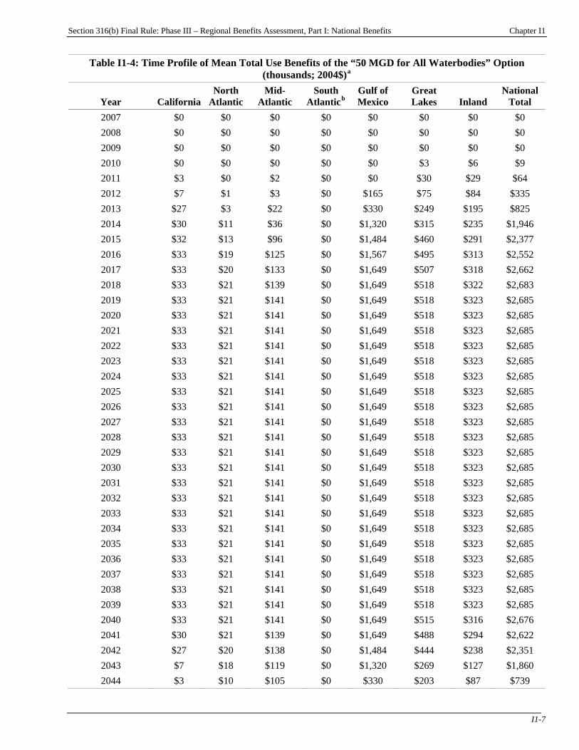
Section 316(b) Final Rule: Phase III – Regional Benefits Assessment, Part I: National Benefits Chapter I1
I1-7
Table I1-4: Time Profile of Mean Total Use Benefits of the “50 MGD for All Waterbodies” Option (thousands; 2004$)P
aP
Year California North
AtlanticMid-
Atlantic South
AtlanticP
bP
Gulf of Mexico
Great Lakes Inland
National Total
2007 $0 $0 $0 $0 $0 $0 $0 $0 2008 $0 $0 $0 $0 $0 $0 $0 $0 2009 $0 $0 $0 $0 $0 $0 $0 $0 2010 $0 $0 $0 $0 $0 $3 $6 $9 2011 $3 $0 $2 $0 $0 $30 $29 $64 2012 $7 $1 $3 $0 $165 $75 $84 $335 2013 $27 $3 $22 $0 $330 $249 $195 $825 2014 $30 $11 $36 $0 $1,320 $315 $235 $1,946 2015 $32 $13 $96 $0 $1,484 $460 $291 $2,377 2016 $33 $19 $125 $0 $1,567 $495 $313 $2,552 2017 $33 $20 $133 $0 $1,649 $507 $318 $2,662 2018 $33 $21 $139 $0 $1,649 $518 $322 $2,683 2019 $33 $21 $141 $0 $1,649 $518 $323 $2,685 2020 $33 $21 $141 $0 $1,649 $518 $323 $2,685 2021 $33 $21 $141 $0 $1,649 $518 $323 $2,685 2022 $33 $21 $141 $0 $1,649 $518 $323 $2,685 2023 $33 $21 $141 $0 $1,649 $518 $323 $2,685 2024 $33 $21 $141 $0 $1,649 $518 $323 $2,685 2025 $33 $21 $141 $0 $1,649 $518 $323 $2,685 2026 $33 $21 $141 $0 $1,649 $518 $323 $2,685 2027 $33 $21 $141 $0 $1,649 $518 $323 $2,685 2028 $33 $21 $141 $0 $1,649 $518 $323 $2,685 2029 $33 $21 $141 $0 $1,649 $518 $323 $2,685 2030 $33 $21 $141 $0 $1,649 $518 $323 $2,685 2031 $33 $21 $141 $0 $1,649 $518 $323 $2,685 2032 $33 $21 $141 $0 $1,649 $518 $323 $2,685 2033 $33 $21 $141 $0 $1,649 $518 $323 $2,685 2034 $33 $21 $141 $0 $1,649 $518 $323 $2,685 2035 $33 $21 $141 $0 $1,649 $518 $323 $2,685 2036 $33 $21 $141 $0 $1,649 $518 $323 $2,685 2037 $33 $21 $141 $0 $1,649 $518 $323 $2,685 2038 $33 $21 $141 $0 $1,649 $518 $323 $2,685 2039 $33 $21 $141 $0 $1,649 $518 $323 $2,685 2040 $33 $21 $141 $0 $1,649 $515 $316 $2,676 2041 $30 $21 $139 $0 $1,649 $488 $294 $2,622 2042 $27 $20 $138 $0 $1,484 $444 $238 $2,351 2043 $7 $18 $119 $0 $1,320 $269 $127 $1,860 2044 $3 $10 $105 $0 $330 $203 $87 $739
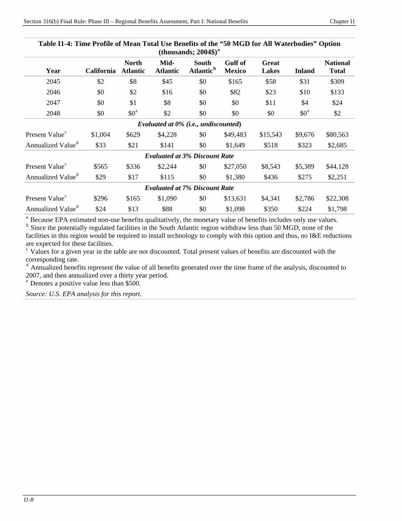
Section 316(b) Final Rule: Phase III – Regional Benefits Assessment, Part I: National Benefits Chapter I1
I1-8
Table I1-4: Time Profile of Mean Total Use Benefits of the “50 MGD for All Waterbodies” Option (thousands; 2004$)P
aP
Year California North
Atlantic Mid-
Atlantic South
AtlanticP
bP
Gulf of Mexico
Great Lakes Inland
National Total
2045 $2 $8 $45 $0 $165 $58 $31 $309 2046 $0 $2 $16 $0 $82 $23 $10 $133 2047 $0 $1 $8 $0 $0 $11 $4 $24 2048 $0 $0P
eP $2 $0 $0 $0 $0P
eP $2
Evaluated at 0% (i.e., undiscounted) Present ValueP
cP $1,004 $629 $4,228 $0 $49,483 $15,543 $9,676 $80,563
Annualized ValueP
dP $33 $21 $141 $0 $1,649 $518 $323 $2,685
Evaluated at 3% Discount Rate Present ValueP
cP $565 $336 $2,244 $0 $27,050 $8,543 $5,389 $44,128
Annualized ValueP
dP $29 $17 $115 $0 $1,380 $436 $275 $2,251
Evaluated at 7% Discount Rate Present ValueP
cP $296 $165 $1,090 $0 $13,631 $4,341 $2,786 $22,308
Annualized ValueP
dP $24 $13 $88 $0 $1,098 $350 $224 $1,798
P
aP Because EPA estimated non-use benefits qualitatively, the monetary value of benefits includes only use values.
P
bP Since the potentially regulated facilities in the South Atlantic region withdraw less than 50 MGD, none of the
facilities in this region would be required to install technology to comply with this option and thus, no I&E reductions are expected for these facilities. P
cP Values for a given year in the table are not discounted. Total present values of benefits are discounted with the
corresponding rate. P
dP Annualized benefits represent the value of all benefits generated over the time frame of the analysis, discounted to
2007, and then annualized over a thirty year period. P
eP Denotes a positive value less than $500.
Source: U.S. EPA analysis for this report.
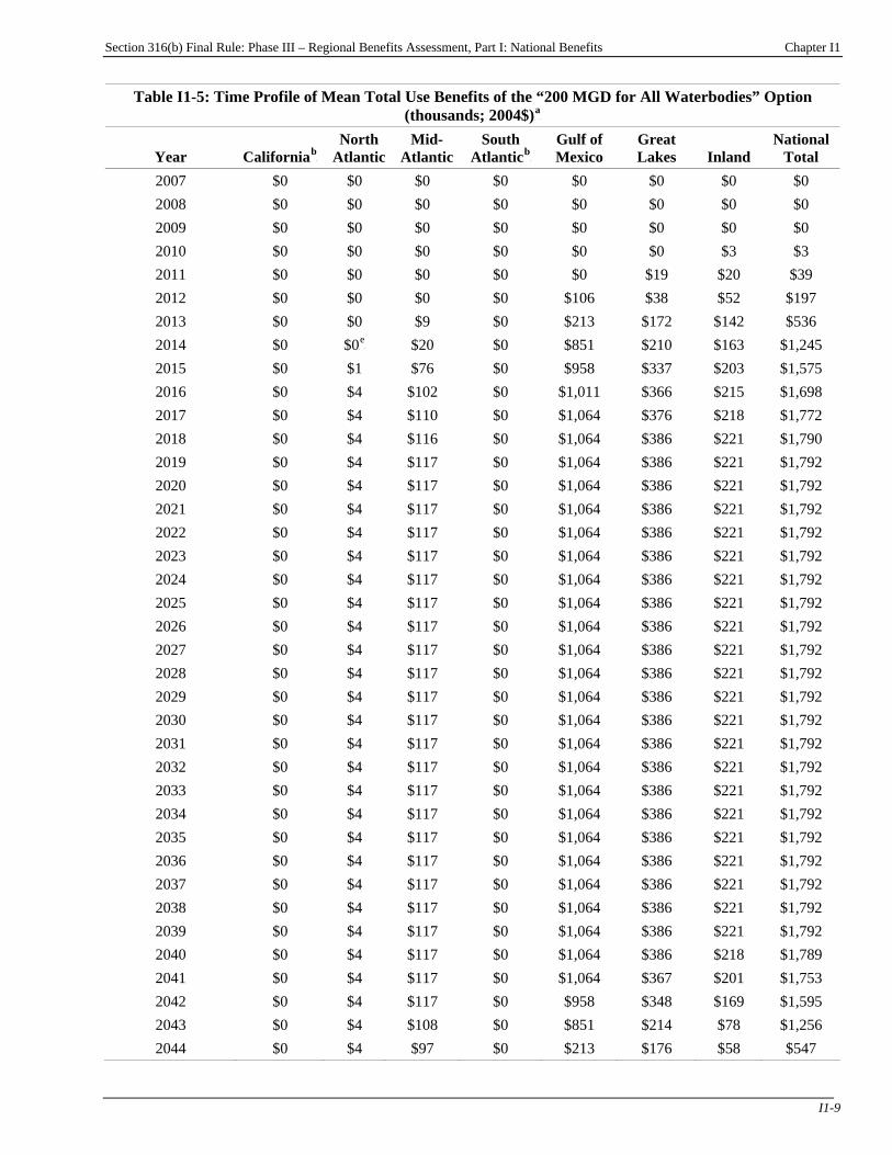
Section 316(b) Final Rule: Phase III – Regional Benefits Assessment, Part I: National Benefits Chapter I1
I1-9
Table I1-5: Time Profile of Mean Total Use Benefits of the “200 MGD for All Waterbodies” Option (thousands; 2004$)P
aP
Year CaliforniaP
bP
North Atlantic
Mid-Atlantic
South AtlanticP
bP
Gulf of Mexico
Great Lakes Inland
National Total
2007 $0 $0 $0 $0 $0 $0 $0 $0 2008 $0 $0 $0 $0 $0 $0 $0 $0 2009 $0 $0 $0 $0 $0 $0 $0 $0 2010 $0 $0 $0 $0 $0 $0 $3 $3 2011 $0 $0 $0 $0 $0 $19 $20 $39 2012 $0 $0 $0 $0 $106 $38 $52 $197 2013 $0 $0 $9 $0 $213 $172 $142 $536 2014 $0 $0P
eP $20 $0 $851 $210 $163 $1,245
2015 $0 $1 $76 $0 $958 $337 $203 $1,575 2016 $0 $4 $102 $0 $1,011 $366 $215 $1,698 2017 $0 $4 $110 $0 $1,064 $376 $218 $1,772 2018 $0 $4 $116 $0 $1,064 $386 $221 $1,790 2019 $0 $4 $117 $0 $1,064 $386 $221 $1,792 2020 $0 $4 $117 $0 $1,064 $386 $221 $1,792 2021 $0 $4 $117 $0 $1,064 $386 $221 $1,792 2022 $0 $4 $117 $0 $1,064 $386 $221 $1,792 2023 $0 $4 $117 $0 $1,064 $386 $221 $1,792 2024 $0 $4 $117 $0 $1,064 $386 $221 $1,792 2025 $0 $4 $117 $0 $1,064 $386 $221 $1,792 2026 $0 $4 $117 $0 $1,064 $386 $221 $1,792 2027 $0 $4 $117 $0 $1,064 $386 $221 $1,792 2028 $0 $4 $117 $0 $1,064 $386 $221 $1,792 2029 $0 $4 $117 $0 $1,064 $386 $221 $1,792 2030 $0 $4 $117 $0 $1,064 $386 $221 $1,792 2031 $0 $4 $117 $0 $1,064 $386 $221 $1,792 2032 $0 $4 $117 $0 $1,064 $386 $221 $1,792 2033 $0 $4 $117 $0 $1,064 $386 $221 $1,792 2034 $0 $4 $117 $0 $1,064 $386 $221 $1,792 2035 $0 $4 $117 $0 $1,064 $386 $221 $1,792 2036 $0 $4 $117 $0 $1,064 $386 $221 $1,792 2037 $0 $4 $117 $0 $1,064 $386 $221 $1,792 2038 $0 $4 $117 $0 $1,064 $386 $221 $1,792 2039 $0 $4 $117 $0 $1,064 $386 $221 $1,792 2040 $0 $4 $117 $0 $1,064 $386 $218 $1,789 2041 $0 $4 $117 $0 $1,064 $367 $201 $1,753 2042 $0 $4 $117 $0 $958 $348 $169 $1,595 2043 $0 $4 $108 $0 $851 $214 $78 $1,256 2044 $0 $4 $97 $0 $213 $176 $58 $547
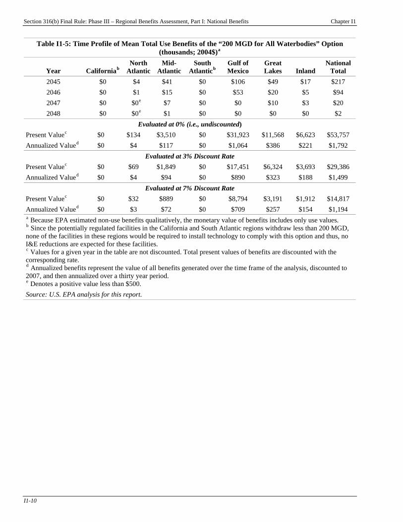
Section 316(b) Final Rule: Phase III – Regional Benefits Assessment, Part I: National Benefits Chapter I1
I1-10
Table I1-5: Time Profile of Mean Total Use Benefits of the “200 MGD for All Waterbodies” Option (thousands; 2004$)P
aP
Year CaliforniaP
bP
North Atlantic
Mid-Atlantic
South AtlanticP
bP
Gulf of Mexico
Great Lakes Inland
National Total
2045 $0 $4 $41 $0 $106 $49 $17 $217 2046 $0 $1 $15 $0 $53 $20 $5 $94 2047 $0 $0P
eP $7 $0 $0 $10 $3 $20
2048 $0 $0P
eP $1 $0 $0 $0 $0 $2
Evaluated at 0% (i.e., undiscounted) Present ValueP
cP $0 $134 $3,510 $0 $31,923 $11,568 $6,623 $53,757
Annualized ValueP
dP $0 $4 $117 $0 $1,064 $386 $221 $1,792
Evaluated at 3% Discount Rate Present ValueP
cP $0 $69 $1,849 $0 $17,451 $6,324 $3,693 $29,386
Annualized ValueP
dP $0 $4 $94 $0 $890 $323 $188 $1,499
Evaluated at 7% Discount Rate Present ValueP
cP $0 $32 $889 $0 $8,794 $3,191 $1,912 $14,817
Annualized ValueP
dP $0 $3 $72 $0 $709 $257 $154 $1,194
P
aP Because EPA estimated non-use benefits qualitatively, the monetary value of benefits includes only use values.
P
bP Since the potentially regulated facilities in the California and South Atlantic regions withdraw less than 200 MGD,
none of the facilities in these regions would be required to install technology to comply with this option and thus, no I&E reductions are expected for these facilities. P
cP Values for a given year in the table are not discounted. Total present values of benefits are discounted with the
corresponding rate. P
dP Annualized benefits represent the value of all benefits generated over the time frame of the analysis, discounted to
2007, and then annualized over a thirty year period. P
eP Denotes a positive value less than $500.
Source: U.S. EPA analysis for this report.
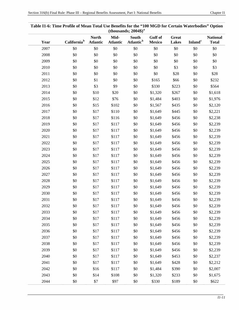
Section 316(b) Final Rule: Phase III – Regional Benefits Assessment, Part I: National Benefits Chapter I1
I1-11
Table I1-6: Time Profile of Mean Total Use Benefits for the “100 MGD for Certain Waterbodies” Option(thousands; 2004$)P
aP
Year CaliforniaP
bP
North Atlantic
Mid-Atlantic
South AtlanticP
bP
Gulf of Mexico
Great Lakes InlandP
cP
National Total
2007 $0 $0 $0 $0 $0 $0 $0 $0 2008 $0 $0 $0 $0 $0 $0 $0 $0 2009 $0 $0 $0 $0 $0 $0 $0 $0 2010 $0 $0 $0 $0 $0 $3 $0 $3 2011 $0 $0 $0 $0 $0 $28 $0 $28 2012 $0 $1 $0 $0 $165 $66 $0 $232 2013 $0 $3 $9 $0 $330 $223 $0 $564 2014 $0 $10 $20 $0 $1,320 $267 $0 $1,618 2015 $0 $12 $76 $0 $1,484 $403 $0 $1,976 2016 $0 $15 $102 $0 $1,567 $435 $0 $2,120 2017 $0 $17 $110 $0 $1,649 $445 $0 $2,221 2018 $0 $17 $116 $0 $1,649 $456 $0 $2,238 2019 $0 $17 $117 $0 $1,649 $456 $0 $2,239 2020 $0 $17 $117 $0 $1,649 $456 $0 $2,239 2021 $0 $17 $117 $0 $1,649 $456 $0 $2,239 2022 $0 $17 $117 $0 $1,649 $456 $0 $2,239 2023 $0 $17 $117 $0 $1,649 $456 $0 $2,239 2024 $0 $17 $117 $0 $1,649 $456 $0 $2,239 2025 $0 $17 $117 $0 $1,649 $456 $0 $2,239 2026 $0 $17 $117 $0 $1,649 $456 $0 $2,239 2027 $0 $17 $117 $0 $1,649 $456 $0 $2,239 2028 $0 $17 $117 $0 $1,649 $456 $0 $2,239 2029 $0 $17 $117 $0 $1,649 $456 $0 $2,239 2030 $0 $17 $117 $0 $1,649 $456 $0 $2,239 2031 $0 $17 $117 $0 $1,649 $456 $0 $2,239 2032 $0 $17 $117 $0 $1,649 $456 $0 $2,239 2033 $0 $17 $117 $0 $1,649 $456 $0 $2,239 2034 $0 $17 $117 $0 $1,649 $456 $0 $2,239 2035 $0 $17 $117 $0 $1,649 $456 $0 $2,239 2036 $0 $17 $117 $0 $1,649 $456 $0 $2,239 2037 $0 $17 $117 $0 $1,649 $456 $0 $2,239 2038 $0 $17 $117 $0 $1,649 $456 $0 $2,239 2039 $0 $17 $117 $0 $1,649 $456 $0 $2,239 2040 $0 $17 $117 $0 $1,649 $453 $0 $2,237 2041 $0 $17 $117 $0 $1,649 $428 $0 $2,212 2042 $0 $16 $117 $0 $1,484 $390 $0 $2,007 2043 $0 $14 $108 $0 $1,320 $233 $0 $1,675 2044 $0 $7 $97 $0 $330 $189 $0 $622
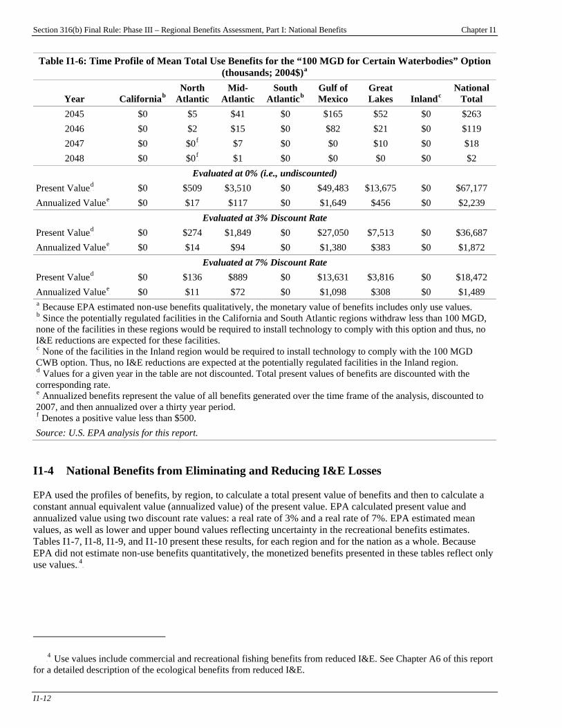
Section 316(b) Final Rule: Phase III – Regional Benefits Assessment, Part I: National Benefits Chapter I1
I1-12
Table I1-6: Time Profile of Mean Total Use Benefits for the “100 MGD for Certain Waterbodies” Option(thousands; 2004$)P
aP
Year CaliforniaP
bP
North Atlantic
Mid-Atlantic
South AtlanticP
bP
Gulf of Mexico
Great Lakes InlandP
cP
National Total
2045 $0 $5 $41 $0 $165 $52 $0 $263 2046 $0 $2 $15 $0 $82 $21 $0 $119 2047 $0 $0P
fP $7 $0 $0 $10 $0 $18
2048 $0 $0P
fP $1 $0 $0 $0 $0 $2
Evaluated at 0% (i.e., undiscounted) Present ValueP
dP $0 $509 $3,510 $0 $49,483 $13,675 $0 $67,177
Annualized ValueP
eP $0 $17 $117 $0 $1,649 $456 $0 $2,239
Evaluated at 3% Discount Rate Present ValueP
dP $0 $274 $1,849 $0 $27,050 $7,513 $0 $36,687
Annualized ValueP
eP $0 $14 $94 $0 $1,380 $383 $0 $1,872
Evaluated at 7% Discount Rate Present ValueP
dP $0 $136 $889 $0 $13,631 $3,816 $0 $18,472
Annualized ValueP
eP $0 $11 $72 $0 $1,098 $308 $0 $1,489
P
aP Because EPA estimated non-use benefits qualitatively, the monetary value of benefits includes only use values.
P
bP Since the potentially regulated facilities in the California and South Atlantic regions withdraw less than 100 MGD,
none of the facilities in these regions would be required to install technology to comply with this option and thus, no I&E reductions are expected for these facilities. P
cP None of the facilities in the Inland region would be required to install technology to comply with the 100 MGD
CWB option. Thus, no I&E reductions are expected at the potentially regulated facilities in the Inland region. P
dP Values for a given year in the table are not discounted. Total present values of benefits are discounted with the
corresponding rate. P
eP Annualized benefits represent the value of all benefits generated over the time frame of the analysis, discounted to
2007, and then annualized over a thirty year period. P
fP Denotes a positive value less than $500.
Source: U.S. EPA analysis for this report. I1-4 National Benefits from Eliminating and Reducing I&E Losses EPA used the profiles of benefits, by region, to calculate a total present value of benefits and then to calculate a constant annual equivalent value (annualized value) of the present value. EPA calculated present value and annualized value using two discount rate values: a real rate of 3% and a real rate of 7%. EPA estimated mean values, as well as lower and upper bound values reflecting uncertainty in the recreational benefits estimates. Tables I1-7, I1-8, I1-9, and I1-10 present these results, for each region and for the nation as a whole. Because EPA did not estimate non-use benefits quantitatively, the monetized benefits presented in these tables reflect only use values.TPF
4FPT
TP
4PT Use values include commercial and recreational fishing benefits from reduced I&E. See Chapter A6 of this report
for a detailed description of the ecological benefits from reduced I&E.

Section 316(b) Final Rule: Phase III – Regional Benefits Assessment, Part I: National Benefits Chapter I1
I1-13
Table I1-7 shows that the total annual national value of fishery resources lost to I&E (i.e., benefits of eliminating baseline I&E losses at Phase III facilities) includes $1.3 million in commercial fishing losses, $6.4 million in recreational fishing losses, and an unknown amount in foregone non-use benefits (2004$, discounted at 3%). The total use value of fishery resources lost is $7.7 million per year, with lower and upper bounds of $5.0 million and $12.6 million, respectively (discounted at 3%). Discounted at 7%, the total annual national value of fishery resources lost to I&E includes $1.3 million in commercial fishing losses, $6.1 million in recreational fishing losses, and an unknown amount in foregone non-use benefits. The total use value of fishery resources lost, discounted at 7%, is $7.3 million per year, with lower and upper bounds of $4.8 million and $12.0 million, respectively. Total monetized losses are greatest in the Gulf of Mexico region. More detailed discussions of the valuation of recreational and commercial fishing losses under the baseline conditions in each region are provided in Parts B through H of this document. Tables I1-8, I1-9 and I1-10 present EPA’s estimates of the national and regional use benefits of reducing I&E under each of the regulatory analysis options (2004$, discounted at 3% and 7%). The national value of these reductions in I&E losses, evaluated at a 3% discount rate, are as follows:
< the “50 MGD for All Waterbodies” option results in national use benefits of $2.3 million per year, with lower and upper bounds of $1.4 million and $3.8 million (see Table I1-8);
< the “200 MGD for All Waterbodies” option results in national use benefits of $1.5 million per year, with lower and upper bounds of $1.0 million and $2.5 million (see Table I1-9); and
< the “100 MGD for Certain Waterbodies” option results in national use benefits of $1.9 million per year, with lower and upper bounds of $1.2 million and $3.1 million (see Table I1-10).
Evaluated at a 7% discount rate, the national use benefits of the regulatory analysis options are somewhat smaller:
< the 50 MGD All option results in national use benefits of $1.8 million per year, with lower and upper bounds of $1.1 million and $3.0 million (see Table I1-8);
< the 200 MGD All option results in national use benefits of $1.2 million per year, with lower and upper bounds of $0.8 million and $2.0 million (see Table I1-9); and
< the 100 MGD CWB option results in national use benefits of $1.5 million per year, with lower and upper bounds of $1.0 million and $2.5 million (see Table I1-10).
The majority of the value of use benefits is attributable to benefits to recreational anglers from improved catch rates. As shown in Tables I1-8, I1-9, and I1-10, use benefits are largest in the Gulf of Mexico for the “50 MGD for All Waterbodies,” “200 MGD for All Waterbodies,” and the “100 MGD for Certain Waterbodies” options. More detailed discussions of regional benefits under each option are provided in Parts B through H of this report.
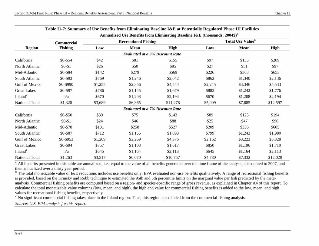
Section 316(b) Final Rule: Phase III – Regional Benefits Assessment, Part I: National Benefits Chapter I1
I1-14
Table I1-7: Summary of Use Benefits from Eliminating Baseline I&E at Potentially Regulated Phase III Facilities Annualized Use Benefits from Eliminating Baseline I&E (thousands; 2004$)P
aP
Recreational Fishing Total Use ValueP
bP
Region Commercial
Fishing Low Mean High Low Mean High Evaluated at a 3% Discount Rate
California $0-$54 $42 $81 $155 $97 $135 $209 North Atlantic $0-$1 $26 $50 $95 $27 $51 $97 Mid-Atlantic $0-$84 $142 $279 $569 $226 $363 $653 South Atlantic $0-$93 $769 $1,246 $2,042 $862 $1,340 $2,136 Gulf of Mexico $0-$990 $1,255 $2,356 $4,544 $2,245 $3,346 $5,533 Great Lakes $0-$97 $786 $1,145 $1,679 $883 $1,242 $1,776 InlandP
cP n/a $670 $1,208 $2,194 $670 $1,208 $2,194
National Total $1,320 $3,689 $6,365 $11,278 $5,009 $7,685 $12,597 Evaluated at a 7% Discount Rate
California $0-$50 $39 $75 $143 $89 $125 $194 North Atlantic $0-$1 $24 $46 $88 $25 $47 $90 Mid-Atlantic $0-$78 $131 $258 $527 $209 $336 $605 South Atlantic $0-$87 $712 $1,155 $1,893 $799 $1,242 $1,980 Gulf of Mexico $0-$953 $1,209 $2,269 $4,376 $2,162 $3,222 $5,328 Great Lakes $0-$94 $757 $1,103 $1,617 $850 $1,196 $1,710 InlandP
cP n/a $645 $1,164 $2,113 $645 $1,164 $2,113
National Total $1,263 $3,517 $6,070 $10,757 $4,780 $7,332 $12,020 P
aP All benefits presented in this table are annualized, i.e., equal to the value of all benefits generated over the time frame of the analysis, discounted to 2007, and
then annualized over a thirty year period. P
bP The total monetizable value of I&E reductions includes use benefits only. EPA evaluated non-use benefits qualitatively. A range of recreational fishing benefits
is provided, based on the Krinsky and Robb technique to estimated the 95th and 5th percentile limits on the marginal value per fish predicted by the meta-analysis. Commercial fishing benefits are computed based on a region- and species-specific range of gross revenue, as explained in Chapter A4 of this report. To calculate the total monetizable value columns (low, mean, and high), the high end value for commercial fishing benefits is added to the low, mean, and high values for recreational fishing benefits, respectively. P
cP No significant commercial fishing takes place in the Inland region. Thus, this region is excluded from the commercial fishing analysis.
Source: U.S. EPA analysis for this report.

Section 316(b) Final Rule: Phase III – Regional Benefits Assessment, Part I: National Benefits Chapter I1
I1-15
Table I1-8: Summary of Use Benefits of the “50 MGD for All Waterbodies” Option (thousands; 2004$)P
aP
Annualized Recreational Fishing Benefits Total Annualized Use BenefitsP
bP
Region Annualized Commercial
Fishing Benefits Low Mean High Low Mean High Evaluated at a 3% Discount Rate
California $0-$8 $11 $21 $40 $19 $29 $48 North Atlantic $0-$0P
eP $9 $17 $33 $9 $17 $33
Mid-Atlantic $0-$18 $48 $96 $198 $67 $115 $216 South AtlanticP
cP $0 $0 $0 $0 $0 $0 $0
Gulf of Mexico $0-$283 $589 $1,097 $2,101 $872 $1,380 $2,384 Great Lakes $0-$11 $292 $425 $624 $302 $436 $634 InlandP
dP n/a $152 $275 $501 $152 $275 $501
National Total $0-$321 $1,101 $1,931 $3,496 $1,421 $2,251 $3,816 Evaluated at a 7% Discount Rate
California $0-$7 $9 $17 $33 $16 $24 $39 North Atlantic $0-$0P
eP $7 $13 $25 $7 $13 $25
Mid-Atlantic $0-$14 $37 $74 $152 $51 $88 $166 South AtlanticP
cP $0 $0 $0 $0 $0 $0 $0
Gulf of Mexico $0-$225 $468 $873 $1,672 $694 $1,098 $1,898 Great Lakes $0-$9 $234 $341 $500 $243 $350 $509 InlandP
dP n/a $124 $224 $409 $124 $224 $409
National Total $0-$255 $880 $1,543 $2,792 $1,135 $1,798 $3,047 P
aP All benefits presented in this table are annualized, i.e., equal to the value of all benefits generated over the time frame of the analysis, discounted to 2007, and
then annualized over a thirty year period. P
bP The total monetizable value of I&E reductions includes use benefits only. EPA evaluated non-use benefits qualitatively. A range of recreational fishing
benefits is provided, based on the Krinsky and Robb technique to estimated the 95th and 5th percentile limits on the marginal value per fish predicted by the meta-analysis. Commercial fishing benefits are computed based on a region- and species-specific range of gross revenue, as explained in Chapter A4 of this report. To calculate the total monetizable value columns (low, mean, and high), the high end value for commercial fishing benefits is added to the low, mean, and high values for recreational fishing benefits, respectively. P
cP Since the potentially regulated facilities in the South Atlantic region withdraw less than 50 MGD, none of the facilities in this region would be required to
install technology to comply with this option and thus, no I&E reductions are expected for these facilities. P
dP No significant commercial fishing takes place in the Inland region. Thus, this region is excluded from the commercial fishing analysis.
P
e PDenotes a positive value less than $500.
Source: U.S. EPA analysis for this report.
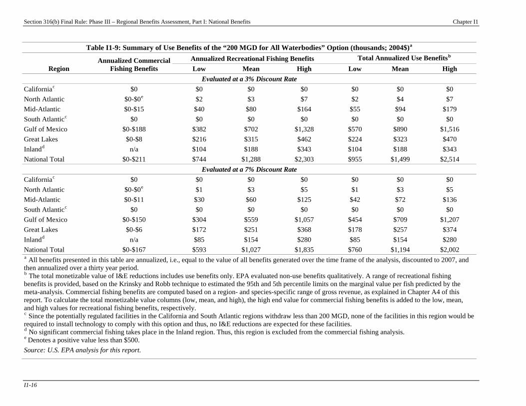
Section 316(b) Final Rule: Phase III – Regional Benefits Assessment, Part I: National Benefits Chapter I1
I1-16
Table I1-9: Summary of Use Benefits of the “200 MGD for All Waterbodies” Option (thousands; 2004$)P
aP
Annualized Recreational Fishing Benefits Total Annualized Use BenefitsP
bP
Region Annualized Commercial
Fishing Benefits Low Mean High Low Mean High Evaluated at a 3% Discount Rate
CaliforniaP
cP $0 $0 $0 $0 $0 $0 $0
North Atlantic $0-$0P
eP $2 $3 $7 $2 $4 $7
Mid-Atlantic $0-$15 $40 $80 $164 $55 $94 $179 South AtlanticP
cP $0 $0 $0 $0 $0 $0 $0
Gulf of Mexico $0-$188 $382 $702 $1,328 $570 $890 $1,516 Great Lakes $0-$8 $216 $315 $462 $224 $323 $470 InlandP
dP n/a $104 $188 $343 $104 $188 $343
National Total $0-$211 $744 $1,288 $2,303 $955 $1,499 $2,514 Evaluated at a 7% Discount Rate
CaliforniaP
cP $0 $0 $0 $0 $0 $0 $0
North Atlantic $0-$0P
eP $1 $3 $5 $1 $3 $5
Mid-Atlantic $0-$11 $30 $60 $125 $42 $72 $136 South AtlanticP
cP $0 $0 $0 $0 $0 $0 $0
Gulf of Mexico $0-$150 $304 $559 $1,057 $454 $709 $1,207 Great Lakes $0-$6 $172 $251 $368 $178 $257 $374 InlandP
dP n/a $85 $154 $280 $85 $154 $280
National Total $0-$167 $593 $1,027 $1,835 $760 $1,194 $2,002 P
aP All benefits presented in this table are annualized, i.e., equal to the value of all benefits generated over the time frame of the analysis, discounted to 2007, and
then annualized over a thirty year period. P
bP The total monetizable value of I&E reductions includes use benefits only. EPA evaluated non-use benefits qualitatively. A range of recreational fishing
benefits is provided, based on the Krinsky and Robb technique to estimated the 95th and 5th percentile limits on the marginal value per fish predicted by the meta-analysis. Commercial fishing benefits are computed based on a region- and species-specific range of gross revenue, as explained in Chapter A4 of this report. To calculate the total monetizable value columns (low, mean, and high), the high end value for commercial fishing benefits is added to the low, mean, and high values for recreational fishing benefits, respectively. P
cP Since the potentially regulated facilities in the California and South Atlantic regions withdraw less than 200 MGD, none of the facilities in this region would be
required to install technology to comply with this option and thus, no I&E reductions are expected for these facilities. P
dP No significant commercial fishing takes place in the Inland region. Thus, this region is excluded from the commercial fishing analysis.
P
e PDenotes a positive value less than $500.
Source: U.S. EPA analysis for this report.
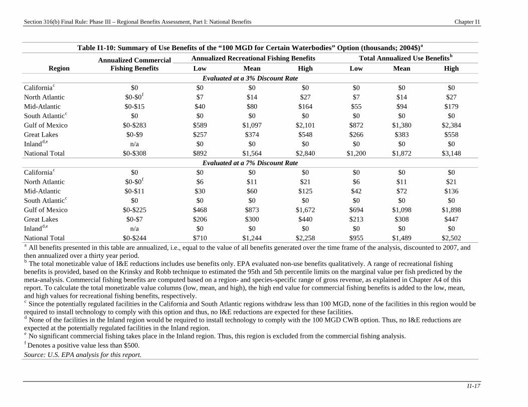
Section 316(b) Final Rule: Phase III – Regional Benefits Assessment, Part I: National Benefits Chapter I1
I1-17
Table I1-10: Summary of Use Benefits of the “100 MGD for Certain Waterbodies” Option (thousands; 2004$)P
aP
Annualized Recreational Fishing Benefits Total Annualized Use BenefitsP
bP
Region Annualized Commercial
Fishing Benefits Low Mean High Low Mean High Evaluated at a 3% Discount Rate
CaliforniaP
cP $0 $0 $0 $0 $0 $0 $0
North Atlantic $0-$0P
fP $7 $14 $27 $7 $14 $27
Mid-Atlantic $0-$15 $40 $80 $164 $55 $94 $179 South AtlanticP
cP $0 $0 $0 $0 $0 $0 $0
Gulf of Mexico $0-$283 $589 $1,097 $2,101 $872 $1,380 $2,384 Great Lakes $0-$9 $257 $374 $548 $266 $383 $558 InlandP
d,eP n/a $0 $0 $0 $0 $0 $0
National Total $0-$308 $892 $1,564 $2,840 $1,200 $1,872 $3,148 Evaluated at a 7% Discount Rate
CaliforniaP
cP $0 $0 $0 $0 $0 $0 $0
North Atlantic $0-$0P
fP $6 $11 $21 $6 $11 $21
Mid-Atlantic $0-$11 $30 $60 $125 $42 $72 $136 South AtlanticP
cP $0 $0 $0 $0 $0 $0 $0
Gulf of Mexico $0-$225 $468 $873 $1,672 $694 $1,098 $1,898 Great Lakes $0-$7 $206 $300 $440 $213 $308 $447 InlandP
d,eP n/a $0 $0 $0 $0 $0 $0
National Total $0-$244 $710 $1,244 $2,258 $955 $1,489 $2,502 P
aP All benefits presented in this table are annualized, i.e., equal to the value of all benefits generated over the time frame of the analysis, discounted to 2007, and
then annualized over a thirty year period. P
bP The total monetizable value of I&E reductions includes use benefits only. EPA evaluated non-use benefits qualitatively. A range of recreational fishing
benefits is provided, based on the Krinsky and Robb technique to estimated the 95th and 5th percentile limits on the marginal value per fish predicted by the meta-analysis. Commercial fishing benefits are computed based on a region- and species-specific range of gross revenue, as explained in Chapter A4 of this report. To calculate the total monetizable value columns (low, mean, and high), the high end value for commercial fishing benefits is added to the low, mean, and high values for recreational fishing benefits, respectively. P
cP Since the potentially regulated facilities in the California and South Atlantic regions withdraw less than 100 MGD, none of the facilities in this region would be
required to install technology to comply with this option and thus, no I&E reductions are expected for these facilities. P
dP None of the facilities in the Inland region would be required to install technology to comply with the 100 MGD CWB option. Thus, no I&E reductions are
expected at the potentially regulated facilities in the Inland region. P
eP No significant commercial fishing takes place in the Inland region. Thus, this region is excluded from the commercial fishing analysis.
P
f PDenotes a positive value less than $500.
Source: U.S. EPA analysis for this report.
Section 316(b) Final Rule: Phase III – Regional Benefits Assessment, Part I: National Benefits Appendix I1
App. I1-1
Appendix I1: National Benefits Under Supplemental Policy Options
Introduction
Appendix Contents I1-1 Summary of Expected Reductions in I&E........ I1-1 I1-2 Total Annualized Monetary Value of
National Losses and Benefits............................ I1-4
This appendix supplements Chapter I1 by presenting EPA’s estimates of the national commercial and recreational benefits of eight supplemental options that EPA evaluated for the purposes of comparison:
< “Electric Generators 2-50 MGD I-only Everywhere” option,
< “Electric Generators 2-50 MGD I&E like Phase II” option, < “Electric Generators 2-50 MGD I&E Everywhere” option, < “Manufacturers 2-50 MGD I-only Everywhere” option, < “Manufacturers 2-50 MGD I&E like Phase II” option, < “Manufacturers 2-50 MGD I&E Everywhere” option, < “Manufacturers 50+ MGD I-only Everywhere” option, and < “Manufacturers 50+ MGD I&E Everywhere” option.
Greater detail on the methods and data used in the regional analyses is provided in the previous chapters of this report. See Chapters A1 and A2 for a discussion of the methods used to estimate I&E, and Chapters A3 through A9 for discussion of the methods used to estimate the value of I&E losses and the benefits of the policy options. The results of the regional analyses are presented in Parts B through H of this report. Chapter I1 presents estimates of national baseline losses and discusses methods used to calculate national benefits under each of the regulatory analysis options. I1-1 Summary of Expected Reductions in I&E Table I1-1 presents the number of facilities with technology requirements under the supplemental evaluated options, by region, and EPA’s estimates of the percentage by which I&E will be reduced under each option. The table also presents estimates of regional and national fishery losses prevented under each option, expressed as age-1 equivalents and fishery yield.
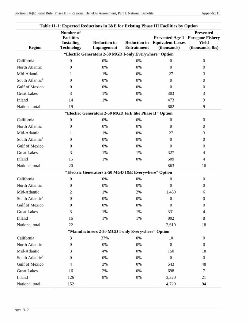
Section 316(b) Final Rule: Phase III – Regional Benefits Assessment, Part I: National Benefits Appendix I1
App. I1-2
Table I1-1: Expected Reductions in I&E for Existing Phase III Facilities by Option
Region
Number of Facilities Installing
Technology Reduction in Impingement
Reduction in Entrainment
Prevented Age-1 Equivalent Losses
(thousands)
Prevented Foregone Fishery
Yield (thousands; lbs)
“Electric Generators 2-50 MGD I-only Everywhere” Option California 0 0% 0% 0 0 North Atlantic 0 0% 0% 0 0 Mid-Atlantic 1 1% 0% 27 3 South AtlanticP
aP 0 0% 0% 0 0
Gulf of Mexico 0 0% 0% 0 0 Great Lakes 3 1% 0% 303 3 Inland 14 1% 0% 473 3 National total 19 802 9
“Electric Generators 2-50 MGD I&E like Phase II” Option California 0 0% 0% 0 0 North Atlantic 0 0% 0% 0 0 Mid-Atlantic 1 1% 0% 27 3 South AtlanticP
aP 0 0% 0% 0 0
Gulf of Mexico 0 0% 0% 0 0 Great Lakes 3 1% 1% 327 4 Inland 15 1% 0% 509 4 National total 20 863 10
“Electric Generators 2-50 MGD I&E Everywhere” Option California 0 0% 0% 0 0 North Atlantic 0 0% 0% 0 0 Mid-Atlantic 2 1% 2% 1,480 6 South AtlanticP
aP 0 0% 0% 0 0
Gulf of Mexico 0 0% 0% 0 0 Great Lakes 3 1% 1% 331 4 Inland 16 1% 1% 802 8 National total 22 2,610 18
“Manufacturers 2-50 MGD I-only Everywhere” Option California 3 37% 0% 10 0 North Atlantic 0 0% 0% 0 0 Mid-Atlantic 3 4% 0% 150 18 South AtlanticP
aP 0 0% 0% 0 0
Gulf of Mexico 4 3% 0% 543 48 Great Lakes 16 2% 0% 698 7 Inland 126 8% 0% 3,320 21 National total 152 4,720 94

Section 316(b) Final Rule: Phase III – Regional Benefits Assessment, Part I: National Benefits Appendix I1
App. I1-3
Table I1-1: Expected Reductions in I&E for Existing Phase III Facilities by Option
Region
Number of Facilities Installing
Technology Reduction in Impingement
Reduction in Entrainment
Prevented Age-1 Equivalent Losses
(thousands)
Prevented Foregone Fishery
Yield (thousands; lbs)
“Manufacturers 2-50 MGD I&E like Phase II” Option California 3 37% 28% 481 34 North Atlantic 0 0% 0% 0 0 Mid-Atlantic 3 4% 3% 2,310 22 South AtlanticP
aP 0 0% 0% 0 0
Gulf of Mexico 4 3% 2% 855 162 Great Lakes 16 2% 1% 732 8 Inland 140 8% 2% 3,660 27 National total 166 8,040 252
“Manufacturers 2-50 MGD I&E Everywhere” Option California 3 37% 31% 534 38 North Atlantic 0 0% 0% 0 0 Mid-Atlantic 3 4% 3% 2,310 22 South AtlanticP
aP 0 0% 0% 0 0
Gulf of Mexico 4 3% 2% 855 162 Great Lakes 16 2% 2% 764 9 Inland 142 8% 7% 4,880 44 National total 168 9,340 275
“Manufacturers 50+ MGD I-only Everywhere” Option California 1 37% 0% 10 0 North Atlantic 0 0% 0% 0 0 Mid-Atlantic 2 23% 0% 1,000 118 South AtlanticP
aP 0 0% 0% 0 0
Gulf of Mexico 5 51% 0% 10,400 917 Great Lakes 15 42% 0% 11,700 109 Inland 74 38% 0% 16,200 105 National total 97 39,400 1,250
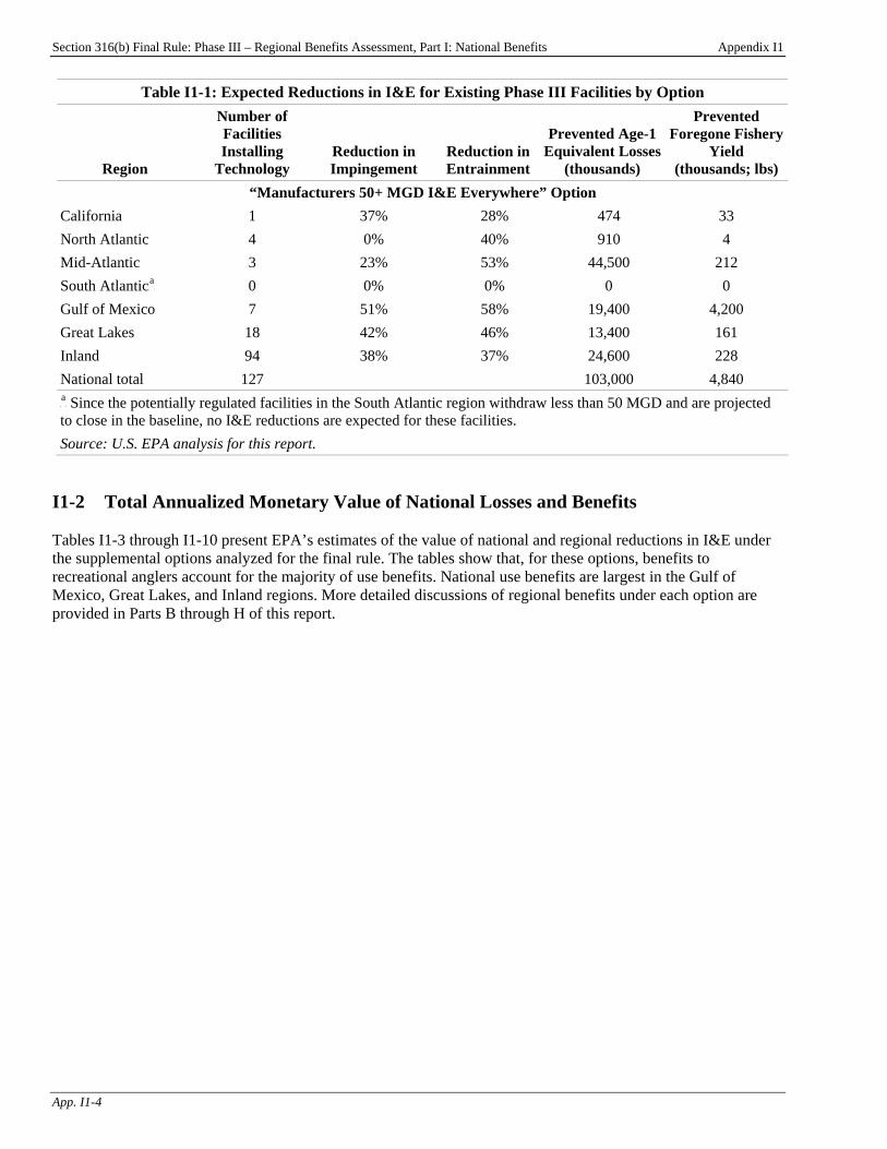
Section 316(b) Final Rule: Phase III – Regional Benefits Assessment, Part I: National Benefits Appendix I1
App. I1-4
Table I1-1: Expected Reductions in I&E for Existing Phase III Facilities by Option
Region
Number of Facilities Installing
Technology Reduction in Impingement
Reduction in Entrainment
Prevented Age-1 Equivalent Losses
(thousands)
Prevented Foregone Fishery
Yield (thousands; lbs)
“Manufacturers 50+ MGD I&E Everywhere” Option California 1 37% 28% 474 33 North Atlantic 4 0% 40% 910 4 Mid-Atlantic 3 23% 53% 44,500 212 South AtlanticP
aP 0 0% 0% 0 0
Gulf of Mexico 7 51% 58% 19,400 4,200 Great Lakes 18 42% 46% 13,400 161 Inland 94 38% 37% 24,600 228 National total 127 103,000 4,840 P
aP Since the potentially regulated facilities in the South Atlantic region withdraw less than 50 MGD and are projected
to close in the baseline, no I&E reductions are expected for these facilities. Source: U.S. EPA analysis for this report.
I1-2 Total Annualized Monetary Value of National Losses and Benefits Tables I1-3 through I1-10 present EPA’s estimates of the value of national and regional reductions in I&E under the supplemental options analyzed for the final rule. The tables show that, for these options, benefits to recreational anglers account for the majority of use benefits. National use benefits are largest in the Gulf of Mexico, Great Lakes, and Inland regions. More detailed discussions of regional benefits under each option are provided in Parts B through H of this report.
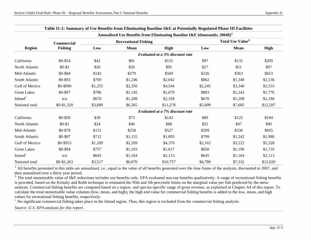
Section 316(b) Final Rule: Phase III – Regional Benefits Assessment, Part I: National Benefits Appendix I1
App. I1-5
Table I1-2: Summary of Use Benefits from Eliminating Baseline I&E at Potentially Regulated Phase III Facilities Annualized Use Benefits from Eliminating Baseline I&E (thousands; 2004$)P
aP
Recreational Fishing Total Use ValueP
bP
Region Commercial
Fishing Low Mean High Low Mean High Evaluated at a 3% discount rate
California $0-$54 $42 $81 $155 $97 $135 $209 North Atlantic $0-$1 $26 $50 $95 $27 $51 $97 Mid-Atlantic $0-$84 $142 $279 $569 $226 $363 $653 South Atlantic $0-$93 $769 $1,246 $2,042 $862 $1,340 $2,136 Gulf of Mexico $0-$990 $1,255 $2,356 $4,544 $2,245 $3,346 $5,533 Great Lakes $0-$97 $786 $1,145 $1,679 $883 $1,242 $1,776 InlandP
cP n/a $670 $1,208 $2,194 $670 $1,208 $2,194
National total $0-$1,320 $3,689 $6,365 $11,278 $5,009 $7,685 $12,597 Evaluated at a 7% discount rate
California $0-$50 $39 $75 $143 $89 $125 $194 North Atlantic $0-$1 $24 $46 $88 $25 $47 $90 Mid-Atlantic $0-$78 $131 $258 $527 $209 $336 $605 South Atlantic $0-$87 $712 $1,155 $1,893 $799 $1,242 $1,980 Gulf of Mexico $0-$953 $1,209 $2,269 $4,376 $2,162 $3,222 $5,328 Great Lakes $0-$94 $757 $1,103 $1,617 $850 $1,196 $1,710 InlandP
cP n/a $645 $1,164 $2,113 $645 $1,164 $2,113
National total $0-$1,263 $3,517 $6,070 $10,757 $4,780 $7,332 $12,020 P
aP All benefits presented in this table are annualized, i.e., equal to the value of all benefits generated over the time frame of the analysis, discounted to 2007, and
then annualized over a thirty year period. P
bP The total monetizable value of I&E reductions includes use benefits only. EPA evaluated non-use benefits qualitatively. A range of recreational fishing benefits
is provided, based on the Krinsky and Robb technique to estimated the 95th and 5th percentile limits on the marginal value per fish predicted by the meta-analysis. Commercial fishing benefits are computed based on a region- and species-specific range of gross revenue, as explained in Chapter A4 of this report. To calculate the total monetizable value columns (low, mean, and high), the high end value for commercial fishing benefits is added to the low, mean, and high values for recreational fishing benefits, respectively. P
cP No significant commercial fishing takes place in the Inland region. Thus, this region is excluded from the commercial fishing analysis.
Source: U.S. EPA analysis for this report.
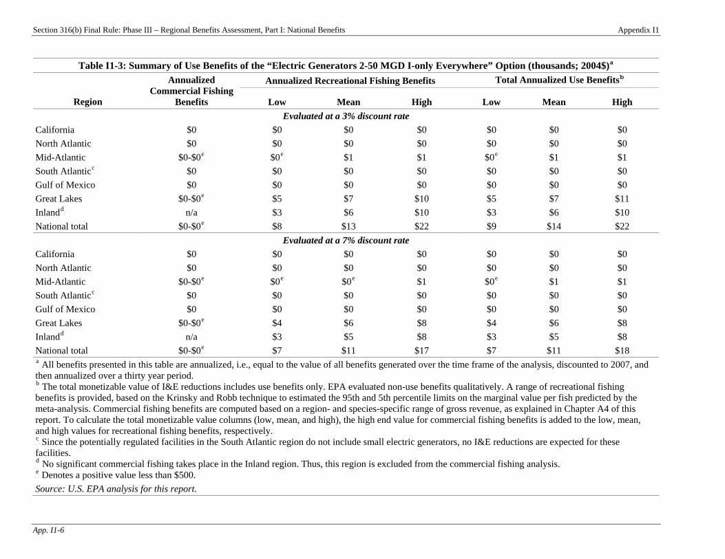
Section 316(b) Final Rule: Phase III – Regional Benefits Assessment, Part I: National Benefits Appendix I1
App. I1-6
Table I1-3: Summary of Use Benefits of the “Electric Generators 2-50 MGD I-only Everywhere” Option (thousands; 2004$)P
aP
Annualized Recreational Fishing Benefits Total Annualized Use BenefitsP
bP
Region
Annualized Commercial Fishing
Benefits Low Mean High Low Mean High Evaluated at a 3% discount rate
California $0 $0 $0 $0 $0 $0 $0 North Atlantic $0 $0 $0 $0 $0 $0 $0 Mid-Atlantic $0-$0P
eP $0P
eP $1 $1 $0P
eP $1 $1
South AtlanticP
cP $0 $0 $0 $0 $0 $0 $0
Gulf of Mexico $0 $0 $0 $0 $0 $0 $0 Great Lakes $0-$0P
eP $5 $7 $10 $5 $7 $11
InlandP
dP n/a $3 $6 $10 $3 $6 $10
National total $0-$0P
eP $8 $13 $22 $9 $14 $22
Evaluated at a 7% discount rate California $0 $0 $0 $0 $0 $0 $0 North Atlantic $0 $0 $0 $0 $0 $0 $0 Mid-Atlantic $0-$0P
eP $0P
eP $0P
eP $1 $0P
eP $1 $1
South AtlanticP
cP $0 $0 $0 $0 $0 $0 $0
Gulf of Mexico $0 $0 $0 $0 $0 $0 $0 Great Lakes $0-$0P
eP $4 $6 $8 $4 $6 $8
InlandP
dP n/a $3 $5 $8 $3 $5 $8
National total $0-$0P
eP $7 $11 $17 $7 $11 $18
P
aP All benefits presented in this table are annualized, i.e., equal to the value of all benefits generated over the time frame of the analysis, discounted to 2007, and
then annualized over a thirty year period. P
bP The total monetizable value of I&E reductions includes use benefits only. EPA evaluated non-use benefits qualitatively. A range of recreational fishing
benefits is provided, based on the Krinsky and Robb technique to estimated the 95th and 5th percentile limits on the marginal value per fish predicted by the meta-analysis. Commercial fishing benefits are computed based on a region- and species-specific range of gross revenue, as explained in Chapter A4 of this report. To calculate the total monetizable value columns (low, mean, and high), the high end value for commercial fishing benefits is added to the low, mean, and high values for recreational fishing benefits, respectively. P
cP Since the potentially regulated facilities in the South Atlantic region do not include small electric generators, no I&E reductions are expected for these
facilities. P
dP No significant commercial fishing takes place in the Inland region. Thus, this region is excluded from the commercial fishing analysis.
P
eP Denotes a positive value less than $500.
Source: U.S. EPA analysis for this report.
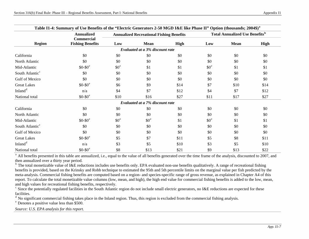
Section 316(b) Final Rule: Phase III – Regional Benefits Assessment, Part I: National Benefits Appendix I1
App. I1-7
Table I1-4: Summary of Use Benefits of the “Electric Generators 2-50 MGD I&E like Phase II” Option (thousands; 2004$)P
aP
Annualized Recreational Fishing Benefits Total Annualized Use BenefitsP
bP
Region
Annualized Commercial
Fishing Benefits Low Mean High Low Mean High Evaluated at a 3% discount rate
California $0 $0 $0 $0 $0 $0 $0 North Atlantic $0 $0 $0 $0 $0 $0 $0 Mid-Atlantic $0-$0P
eP $0P
eP $1 $1 $0P
eP $1 $1
South AtlanticP
cP $0 $0 $0 $0 $0 $0 $0
Gulf of Mexico $0 $0 $0 $0 $0 $0 $0 Great Lakes $0-$0P
eP $6 $9 $14 $7 $10 $14
InlandP
dP n/a $4 $7 $12 $4 $7 $12
National total $0-$0P
eP $10 $16 $27 $11 $17 $27
Evaluated at a 7% discount rate California $0 $0 $0 $0 $0 $0 $0 North Atlantic $0 $0 $0 $0 $0 $0 $0 Mid-Atlantic $0-$0P
eP $0P
eP $0P
eP $1 $0P
eP $1 $1
South AtlanticP
cP $0 $0 $0 $0 $0 $0 $0
Gulf of Mexico $0 $0 $0 $0 $0 $0 $0 Great Lakes $0-$0P
eP $5 $7 $11 $5 $8 $11
InlandP
dP n/a $3 $5 $10 $3 $5 $10
National total $0-$0P
eP $8 $13 $21 $9 $13 $22
P
aP All benefits presented in this table are annualized, i.e., equal to the value of all benefits generated over the time frame of the analysis, discounted to 2007, and
then annualized over a thirty year period. P
bP The total monetizable value of I&E reductions includes use benefits only. EPA evaluated non-use benefits qualitatively. A range of recreational fishing
benefits is provided, based on the Krinsky and Robb technique to estimated the 95th and 5th percentile limits on the marginal value per fish predicted by the meta-analysis. Commercial fishing benefits are computed based on a region- and species-specific range of gross revenue, as explained in Chapter A4 of this report. To calculate the total monetizable value columns (low, mean, and high), the high end value for commercial fishing benefits is added to the low, mean, and high values for recreational fishing benefits, respectively. P
cP Since the potentially regulated facilities in the South Atlantic region do not include small electric generators, no I&E reductions are expected for these
facilities. P
dP No significant commercial fishing takes place in the Inland region. Thus, this region is excluded from the commercial fishing analysis.
P
eP Denotes a positive value less than $500.
Source: U.S. EPA analysis for this report.
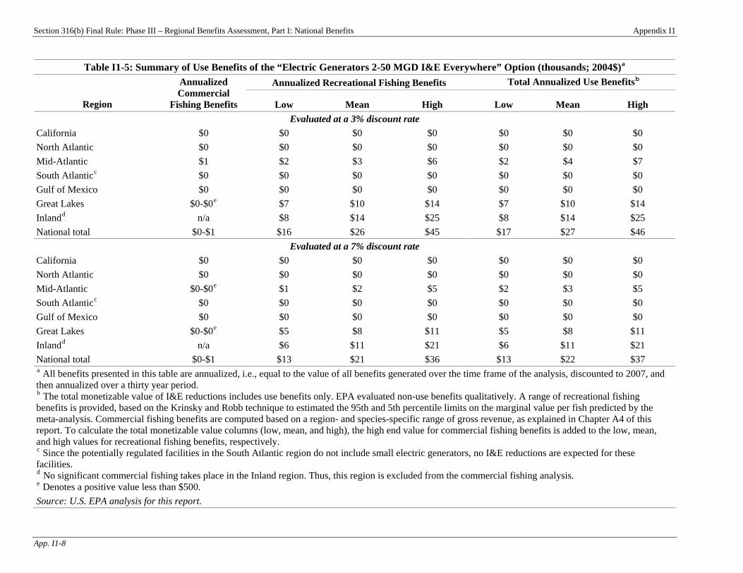
Section 316(b) Final Rule: Phase III – Regional Benefits Assessment, Part I: National Benefits Appendix I1
App. I1-8
Table I1-5: Summary of Use Benefits of the “Electric Generators 2-50 MGD I&E Everywhere” Option (thousands; 2004$)P
aP
Annualized Recreational Fishing Benefits Total Annualized Use BenefitsP
bP
Region
Annualized Commercial
Fishing Benefits Low Mean High Low Mean High Evaluated at a 3% discount rate
California $0 $0 $0 $0 $0 $0 $0 North Atlantic $0 $0 $0 $0 $0 $0 $0 Mid-Atlantic $1 $2 $3 $6 $2 $4 $7 South AtlanticP
cP $0 $0 $0 $0 $0 $0 $0
Gulf of Mexico $0 $0 $0 $0 $0 $0 $0 Great Lakes $0-$0P
eP $7 $10 $14 $7 $10 $14
InlandP
dP n/a $8 $14 $25 $8 $14 $25
National total $0-$1 $16 $26 $45 $17 $27 $46 Evaluated at a 7% discount rate
California $0 $0 $0 $0 $0 $0 $0 North Atlantic $0 $0 $0 $0 $0 $0 $0 Mid-Atlantic $0-$0P
eP $1 $2 $5 $2 $3 $5
South AtlanticP
cP $0 $0 $0 $0 $0 $0 $0
Gulf of Mexico $0 $0 $0 $0 $0 $0 $0 Great Lakes $0-$0P
eP $5 $8 $11 $5 $8 $11
InlandP
dP n/a $6 $11 $21 $6 $11 $21
National total $0-$1 $13 $21 $36 $13 $22 $37 P
aP All benefits presented in this table are annualized, i.e., equal to the value of all benefits generated over the time frame of the analysis, discounted to 2007, and
then annualized over a thirty year period. P
bP The total monetizable value of I&E reductions includes use benefits only. EPA evaluated non-use benefits qualitatively. A range of recreational fishing
benefits is provided, based on the Krinsky and Robb technique to estimated the 95th and 5th percentile limits on the marginal value per fish predicted by the meta-analysis. Commercial fishing benefits are computed based on a region- and species-specific range of gross revenue, as explained in Chapter A4 of this report. To calculate the total monetizable value columns (low, mean, and high), the high end value for commercial fishing benefits is added to the low, mean, and high values for recreational fishing benefits, respectively. P
cP Since the potentially regulated facilities in the South Atlantic region do not include small electric generators, no I&E reductions are expected for these
facilities. P
dP No significant commercial fishing takes place in the Inland region. Thus, this region is excluded from the commercial fishing analysis.
P
eP Denotes a positive value less than $500.
Source: U.S. EPA analysis for this report.
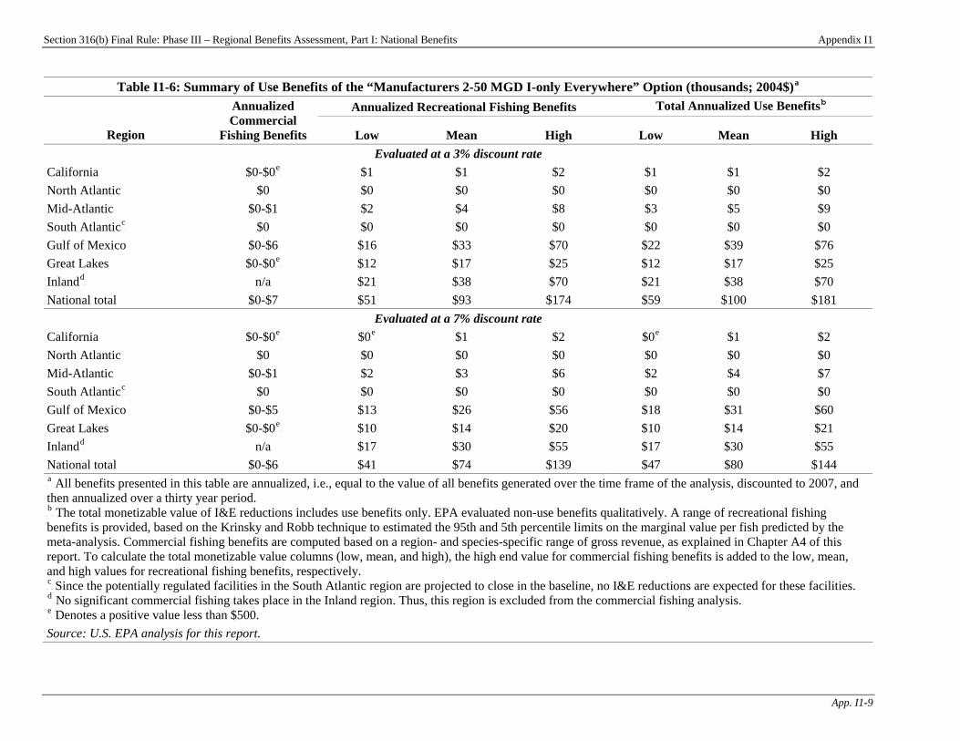
Section 316(b) Final Rule: Phase III – Regional Benefits Assessment, Part I: National Benefits Appendix I1
App. I1-9
Table I1-6: Summary of Use Benefits of the “Manufacturers 2-50 MGD I-only Everywhere” Option (thousands; 2004$)P
aP
Annualized Recreational Fishing Benefits Total Annualized Use BenefitsP
bP
Region
Annualized Commercial
Fishing Benefits Low Mean High Low Mean High Evaluated at a 3% discount rate
California $0-$0P
eP $1 $1 $2 $1 $1 $2
North Atlantic $0 $0 $0 $0 $0 $0 $0 Mid-Atlantic $0-$1 $2 $4 $8 $3 $5 $9 South AtlanticP
cP $0 $0 $0 $0 $0 $0 $0
Gulf of Mexico $0-$6 $16 $33 $70 $22 $39 $76 Great Lakes $0-$0P
eP $12 $17 $25 $12 $17 $25
InlandP
dP n/a $21 $38 $70 $21 $38 $70
National total $0-$7 $51 $93 $174 $59 $100 $181 Evaluated at a 7% discount rate
California $0-$0P
eP $0P
eP $1 $2 $0P
eP $1 $2
North Atlantic $0 $0 $0 $0 $0 $0 $0 Mid-Atlantic $0-$1 $2 $3 $6 $2 $4 $7 South AtlanticP
cP $0 $0 $0 $0 $0 $0 $0
Gulf of Mexico $0-$5 $13 $26 $56 $18 $31 $60 Great Lakes $0-$0P
eP $10 $14 $20 $10 $14 $21
InlandP
dP n/a $17 $30 $55 $17 $30 $55
National total $0-$6 $41 $74 $139 $47 $80 $144 P
aP All benefits presented in this table are annualized, i.e., equal to the value of all benefits generated over the time frame of the analysis, discounted to 2007, and
then annualized over a thirty year period. P
bP The total monetizable value of I&E reductions includes use benefits only. EPA evaluated non-use benefits qualitatively. A range of recreational fishing
benefits is provided, based on the Krinsky and Robb technique to estimated the 95th and 5th percentile limits on the marginal value per fish predicted by the meta-analysis. Commercial fishing benefits are computed based on a region- and species-specific range of gross revenue, as explained in Chapter A4 of this report. To calculate the total monetizable value columns (low, mean, and high), the high end value for commercial fishing benefits is added to the low, mean, and high values for recreational fishing benefits, respectively. P
cP Since the potentially regulated facilities in the South Atlantic region are projected to close in the baseline, no I&E reductions are expected for these facilities.
P
dP No significant commercial fishing takes place in the Inland region. Thus, this region is excluded from the commercial fishing analysis.
P
eP Denotes a positive value less than $500.
Source: U.S. EPA analysis for this report.
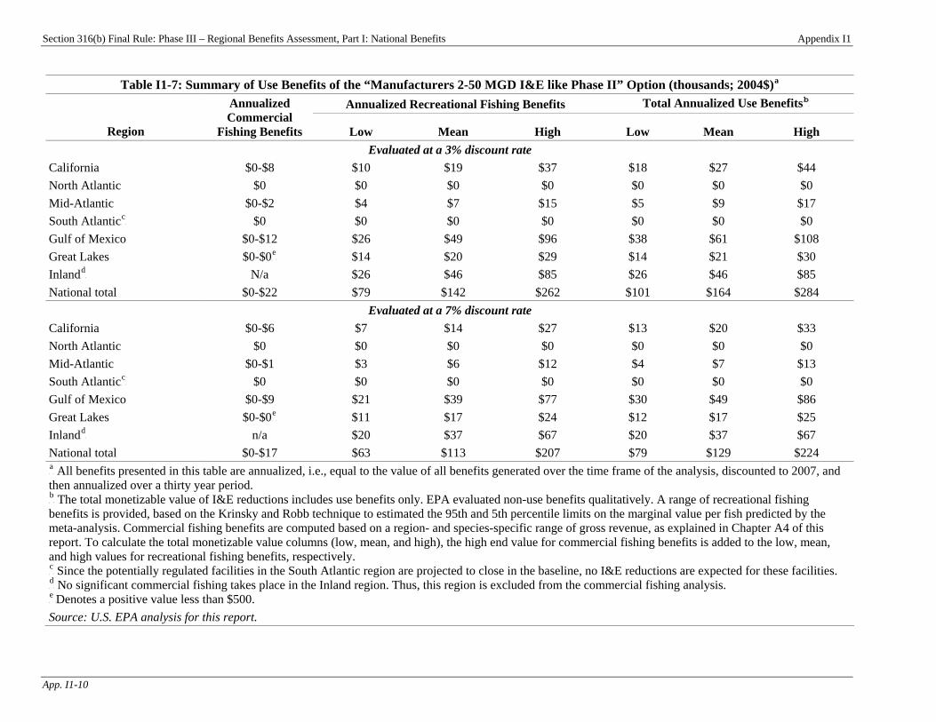
Section 316(b) Final Rule: Phase III – Regional Benefits Assessment, Part I: National Benefits Appendix I1
App. I1-10
Table I1-7: Summary of Use Benefits of the “Manufacturers 2-50 MGD I&E like Phase II” Option (thousands; 2004$)P
aP
Annualized Recreational Fishing Benefits Total Annualized Use BenefitsP
bP
Region
Annualized Commercial
Fishing Benefits Low Mean High Low Mean High Evaluated at a 3% discount rate
California $0-$8 $10 $19 $37 $18 $27 $44 North Atlantic $0 $0 $0 $0 $0 $0 $0 Mid-Atlantic $0-$2 $4 $7 $15 $5 $9 $17 South AtlanticP
cP $0 $0 $0 $0 $0 $0 $0
Gulf of Mexico $0-$12 $26 $49 $96 $38 $61 $108 Great Lakes $0-$0P
eP $14 $20 $29 $14 $21 $30
InlandP
dP N/a $26 $46 $85 $26 $46 $85
National total $0-$22 $79 $142 $262 $101 $164 $284 Evaluated at a 7% discount rate
California $0-$6 $7 $14 $27 $13 $20 $33 North Atlantic $0 $0 $0 $0 $0 $0 $0 Mid-Atlantic $0-$1 $3 $6 $12 $4 $7 $13 South AtlanticP
cP $0 $0 $0 $0 $0 $0 $0
Gulf of Mexico $0-$9 $21 $39 $77 $30 $49 $86 Great Lakes $0-$0P
eP $11 $17 $24 $12 $17 $25
InlandP
dP n/a $20 $37 $67 $20 $37 $67
National total $0-$17 $63 $113 $207 $79 $129 $224 P
aP All benefits presented in this table are annualized, i.e., equal to the value of all benefits generated over the time frame of the analysis, discounted to 2007, and
then annualized over a thirty year period. P
bP The total monetizable value of I&E reductions includes use benefits only. EPA evaluated non-use benefits qualitatively. A range of recreational fishing
benefits is provided, based on the Krinsky and Robb technique to estimated the 95th and 5th percentile limits on the marginal value per fish predicted by the meta-analysis. Commercial fishing benefits are computed based on a region- and species-specific range of gross revenue, as explained in Chapter A4 of this report. To calculate the total monetizable value columns (low, mean, and high), the high end value for commercial fishing benefits is added to the low, mean, and high values for recreational fishing benefits, respectively. P
cP Since the potentially regulated facilities in the South Atlantic region are projected to close in the baseline, no I&E reductions are expected for these facilities.
P
dP No significant commercial fishing takes place in the Inland region. Thus, this region is excluded from the commercial fishing analysis.
P
e PDenotes a positive value less than $500.
Source: U.S. EPA analysis for this report.

Section 316(b) Final Rule: Phase III – Regional Benefits Assessment, Part I: National Benefits Appendix I1
App. I1-11
Table I1-8: Summary of Use Benefits of the “Manufacturers 2-50 MGD I&E Everywhere” Option (thousands; 2004$)P
aP
Annualized Recreational Fishing Benefits Total Annualized Use BenefitsP
bP
Region
Annualized Commercial
Fishing Benefits Low Mean High Low Mean High Evaluated at a 3% discount rate
California $0-$8 $11 $21 $41 $20 $30 $49 North Atlantic $0 $0 $0 $0 $0 $0 $0 Mid-Atlantic $0-$2 $4 $7 $15 $5 $9 $17 South AtlanticP
cP $0 $0 $0 $0 $0 $0 $0
Gulf of Mexico $0-$12 $26 $49 $96 $38 $61 $108 Great Lakes $0-$1 $16 $23 $34 $16 $24 $35 InlandP
dP n/a $42 $76 $138 $42 $76 $138
National total $0-$22 $99 $177 $324 $121 $199 $346 Evaluated at a 7% discount rate
California $0-$6 $8 $16 $30 $14 $22 $36 North Atlantic $0 $0 $0 $0 $0 $0 $0 Mid-Atlantic $0-$1 $3 $6 $12 $4 $7 $13 South AtlanticP
cP $0 $0 $0 $0 $0 $0 $0
Gulf of Mexico $0-$9 $21 $39 $77 $30 $49 $86 Great Lakes $0-$0P
eP $13 $19 $28 $14 $20 $28
InlandP
dP n/a $33 $60 $109 $33 $60 $109
National total $0-$17 $78 $140 $256 $96 $157 $273 P
aP All benefits presented in this table are annualized, i.e., equal to the value of all benefits generated over the time frame of the analysis, discounted to 2007, and
then annualized over a thirty year period. P
bP The total monetizable value of I&E reductions includes use benefits only. EPA evaluated non-use benefits qualitatively. A range of recreational fishing
benefits is provided, based on the Krinsky and Robb technique to estimated the 95th and 5th percentile limits on the marginal value per fish predicted by the meta-analysis. Commercial fishing benefits are computed based on a region- and species-specific range of gross revenue, as explained in Chapter A4 of this report. To calculate the total monetizable value columns (low, mean, and high), the high end value for commercial fishing benefits is added to the low, mean, and high values for recreational fishing benefits, respectively. P
cP Since the potentially regulated facilities in the South Atlantic region are projected to close in the baseline, no I&E reductions are expected for these facilities.
P
dP No significant commercial fishing takes place in the Inland region. Thus, this region is excluded from the commercial fishing analysis.
P
e PDenotes a positive value less than $500.
Source: U.S. EPA analysis for this report.
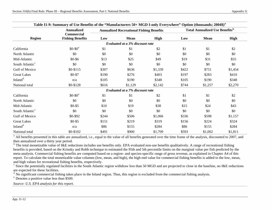
Section 316(b) Final Rule: Phase III – Regional Benefits Assessment, Part I: National Benefits Appendix I1
App. I1-12
Table I1-9: Summary of Use Benefits of the “Manufacturers 50+ MGD I-only Everywhere” Option (thousands; 2004$)P
aP
Annualized Recreational Fishing Benefits Total Annualized Use BenefitsP
bP
Region
Annualized Commercial
Fishing Benefits Low Mean High Low Mean High Evaluated at a 3% discount rate
California $0-$0P
eP $1 $1 $2 $1 $1 $2
North Atlantic $0 $0 $0 $0 $0 $0 $0 Mid-Atlantic $0-$6 $13 $25 $49 $19 $31 $55 South AtlanticP
cP $0 $0 $0 $0 $0 $0 $0
Gulf of Mexico $0-$115 $307 $636 $1,339 $422 $751 $1,454 Great Lakes $0-$7 $190 $276 $403 $197 $283 $410 InlandP
dP n/a $105 $190 $348 $105 $190 $348
National total $0-$128 $616 $1,129 $2,142 $744 $1,257 $2,270 Evaluated at a 7% discount rate
California $0-$0P
eP $1 $1 $2 $1 $1 $2
North Atlantic $0 $0 $0 $0 $0 $0 $0 Mid-Atlantic $0-$5 $10 $19 $38 $15 $24 $43 South AtlanticP
cP $0 $0 $0 $0 $0 $0 $0
Gulf of Mexico $0-$92 $244 $506 $1,066 $336 $598 $1,157 Great Lakes $0-$5 $151 $219 $319 $156 $224 $324 InlandP
dP n/a $86 $155 $284 $86 $155 $284
National total $0-$102 $491 $900 $1,709 $593 $1,002 $1,811 P
aP All benefits presented in this table are annualized, i.e., equal to the value of all benefits generated over the time frame of the analysis, discounted to 2007, and
then annualized over a thirty year period. P
bP The total monetizable value of I&E reductions includes use benefits only. EPA evaluated non-use benefits qualitatively. A range of recreational fishing
benefits is provided, based on the Krinsky and Robb technique to estimated the 95th and 5th percentile limits on the marginal value per fish predicted by the meta-analysis. Commercial fishing benefits are computed based on a region- and species-specific range of gross revenue, as explained in Chapter A4 of this report. To calculate the total monetizable value columns (low, mean, and high), the high end value for commercial fishing benefits is added to the low, mean, and high values for recreational fishing benefits, respectively. P
cP Since the potentially regulated facilities in the South Atlantic region withdraw less than 50 MGD and are projected to close in the baseline, no I&E reductions
are expected for these facilities. P
dP No significant commercial fishing takes place in the Inland region. Thus, this region is excluded from the commercial fishing analysis.
P
eP Denotes a positive value less than $500.
Source: U.S. EPA analysis for this report.
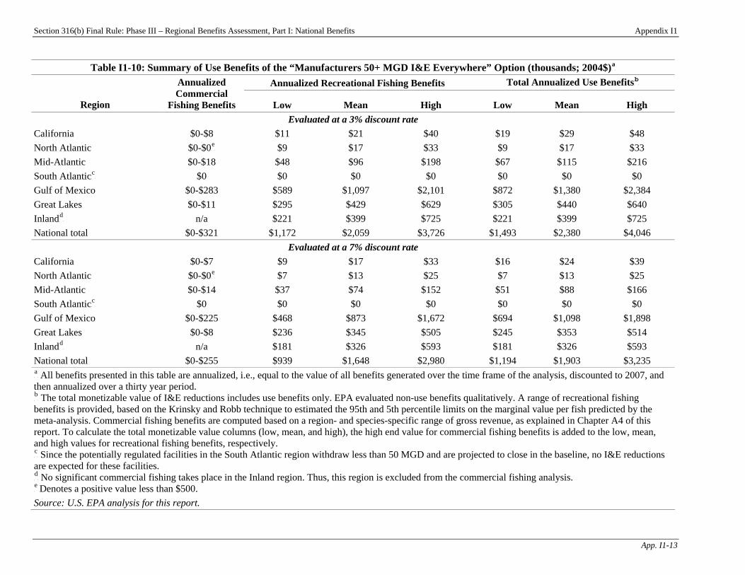
Section 316(b) Final Rule: Phase III – Regional Benefits Assessment, Part I: National Benefits Appendix I1
Table I1-10: Summary of Use Benefits of the “Manufacturers 50+ MGD I&E Everywhere” Option (thousands; 2004$)P
aP
Annualized Recreational Fishing Benefits Total Annualized Use BenefitsP
bP
Region
Annualized Commercial
Fishing Benefits Low Mean High Low Mean High Evaluated at a 3% discount rate
California $0-$8 $11 $21 $40 $19 $29 $48 North Atlantic $0-$0P
eP $9 $17 $33 $9 $17 $33
Mid-Atlantic $0-$18 $48 $96 $198 $67 $115 $216 South AtlanticP
cP $0 $0 $0 $0 $0 $0 $0
Gulf of Mexico $0-$283 $589 $1,097 $2,101 $872 $1,380 $2,384 Great Lakes $0-$11 $295 $429 $629 $305 $440 $640 InlandP
dP n/a $221 $399 $725 $221 $399 $725
National total $0-$321 $1,172 $2,059 $3,726 $1,493 $2,380 $4,046 Evaluated at a 7% discount rate
California $0-$7 $9 $17 $33 $16 $24 $39 North Atlantic $0-$0P
eP $7 $13 $25 $7 $13 $25
Mid-Atlantic $0-$14 $37 $74 $152 $51 $88 $166 South AtlanticP
cP $0 $0 $0 $0 $0 $0 $0
Gulf of Mexico $0-$225 $468 $873 $1,672 $694 $1,098 $1,898 Great Lakes $0-$8 $236 $345 $505 $245 $353 $514 InlandP
dP n/a $181 $326 $593 $181 $326 $593
National total $0-$255 $939 $1,648 $2,980 $1,194 $1,903 $3,235 P
aP All benefits presented in this table are annualized, i.e., equal to the value of all benefits generated over the time frame of the analysis, discounted to 2007, and
then annualized over a thirty year period. P
bP The total monetizable value of I&E reductions includes use benefits only. EPA evaluated non-use benefits qualitatively. A range of recreational fishing
benefits is provided, based on the Krinsky and Robb technique to estimated the 95th and 5th percentile limits on the marginal value per fish predicted by the meta-analysis. Commercial fishing benefits are computed based on a region- and species-specific range of gross revenue, as explained in Chapter A4 of this report. To calculate the total monetizable value columns (low, mean, and high), the high end value for commercial fishing benefits is added to the low, mean, and high values for recreational fishing benefits, respectively. P
cP Since the potentially regulated facilities in the South Atlantic region withdraw less than 50 MGD and are projected to close in the baseline, no I&E reductions
are expected for these facilities. P
dP No significant commercial fishing takes place in the Inland region. Thus, this region is excluded from the commercial fishing analysis.
P
e PDenotes a positive value less than $500.
Source: U.S. EPA analysis for this report.
App. I1-13
Section 316(b) Final Rule: Phase III – Regional Benefits Assessment References
Ref-1
References Able, K.W. and M.P. Fahay. 1998. The First Year in the Life of Estuarine Fishes in the Middle Atlantic Bight. Rutgers University Press, New Brunswick, NJ. Abt Associates. 2006. Development of Willingness to Pay Survey Instrument for Section 316(b) Phase III Cooling Water Intake Structures. Memorandum to Julie Hewitt, OW/OST/EAD dated May 23, 2006. Abt Associates, Inc., Cambridge, MA. Agnello, R. 1989. The economic value of fishing success: An application of socioeconomic survey data. Fishery Bulletin 87(1):223-232. Alexander, S.J. 1995. Applying Random Utility Modeling to Recreational Fishing in Oregon: Effects of Forest Management Alternatives on Steelhead Production in the Elk River Watershed. Oregon State University. Allen, M.A. and T.J. Hassler. 1986. Species Profiles: Life Histories and Environmental Requirements of Coastal Fishes and Invertebrates (Pacific Southwest) — Chinook Salmon. U.S. Fish and Wildlife Service Biological Report 82(11.49). U.S. Army Corps of Engineers TR EL-82-4. http://www.nwrc.gov/publications/specintro.htm. Accessed 7/03. Anderson, L.G. 1980. Necessary components of economic surplus in fisheries economics. Canadian Journal of Fisheries and Aquatic Sciences 37:858-870. Arrow, K., R. Solow, P. Portney, E. Leamer, R. Radner, and H. Schuman. 1993. Report of the NOAA panel on contingent valuation. Federal Register 58(10):4602-4614. ASMFC. 2001a. Interstate Fisheries Management Program: Atlantic Herring. Atlantic States Marine Fisheries Commission. http://www.asmfc.org/Programs/Fish%20Mgnt/AHERRING1.html. Accessed 2/12/01. ASMFC. 2001b. Review of the Fishery Management Plan for Atlantic Menhaden. Atlantic States Marine Fisheries Commission. http://www.asmfc.org/Programs/Fish%20Mgnt/2000%20FMP%20Reviews/menhaden2000_FMP.HTM. Accessed 3/19/01. Bartell, S.M. and K.R. Campbell. 2000. Ecological Risk Assessment of the Effects of the Incremental Increase of Commercial Navigation Traffic (25, 50, 75, and 100 Percent Increase of 1992 Baseline Traffic) on Fish. ENV Report 16. Prepared for U.S. Army Engineer District, Rock Island. July. http://www.mvr.usace.army.mil/pdw/nav_study/env_reports/ENVRPT16.htm. Accessed 2000. Bason, W.H. 1971. Ecology and early life history of striped bass, Morone saxatilis, in the Delaware Estuary. Ichthyol. Assoc. Bulletin 4:112. Ichthyological Associates, Middletown, DE. Bateman, I.J. and A.P. Jones. 2003. Contrasting conventional with multi-level modeling approaches to meta-analysis: Expectation consistency in U.K. woodland recreation values. Land Economics 79(2):235-258. Bateman, I.J., R.T. Carson, B. Day, M. Hanemann, N. Hanley, T. Hett, M. Jones-Lee, G. Loomes, S. Mourato, E. Ozdemiroglu, D.W. Pierce, R. Sugden, and J. Swanson. 2002. Economic Valuation with Stated Preference Surveys: A Manual. Edward Elgar, Northampton, MA. BEA. 1998. Bureau of Economic Analysis National Accounts Data: Gross Product by Industry. http://www.bea.doc.gov/bea/dn2/gpoc.htm.
Section 316(b) Final Rule: Phase III – Regional Benefits Assessment References
Ref-2
Beauchamp, D.A., M.F. Shepard, and G.B. Pauley. 1983. Species Profiles: Life Histories and Environmental Requirements of Coastal Fishes and Invertebrates (Pacific Northwest): Chinook Salmon. U.S. Fish and Wildlife Service FWS/OBS-82/11.6. U.S. Army Corps of Engineers TR EL-82-4. Beck, A.D. and the Committee on Entrainment. 1978. Cumulative effects: A field assessment. In Power Plant Entrainment: A Biological Assessment, J.R. Schubel and B.C. Marcy, Jr. (eds.). Academic Press, New York, pp. 189-210. Bergstrom, J.C. and P. De Civita. 1999. Status of benefits transfer in the United States and Canada: A review. Canadian Journal of Agricultural Economics 47(1):79-87. Berman, M., S. Haley, and H. Kim. 1997. Estimating net benefits of reallocation: Discrete choice models of sport and commercial fishing. Marine Resource Economics 12:307-327. Berrens, R.P., O. Bergland, and R.M. Adams. 1993. Valuation issues in an urban recreational fishery: Spring chinook salmon in Portland, Oregon. Journal of Leisure Research Vol 25. Berrens, R.P., P. Ganderston, and C.L. Silva. 1996. Valuing the protection of minimum instream flows in New Mexico. Journal of Agricultural and Resource Economics 21(2):294-309. Bert, T.M., R.E. Warner, and L.D. Kessler. 1978. The Biology and Florida Fishery of the Stone Crab, Menippe mercenaria (Say), with Emphasis on Southwest Florida. Technical Paper No. 9. State University System of Florida Sea College Program, Gainesville. October. Besedin, E., M. Ranson, and R. Johnston. 2004a. Findings from Focus Groups. Memo to U.S. EPA/OW, Appendices I-III, Focus Group Transcripts. Besedin, E., R. Johnston, M. Ranson, and J. Ahlen. 2005. Findings from 2005 Focus Groups Conducted Under EPA ICR #2155.02. Besedin, E., M. Mazzotta, D. Cacela, and L. Tudor. 2004b. Combining Ecological and Economic Analysis: An Application to Valuation of Power Plant Impacts on Great Lakes Recreational Fishing. Paper Presented at American Fisheries Society Meeting Symposium: Socio-economics and Extension: Empowering People in Fisheries Conservation. August. Bielsa, L.M., W.H. Murdich, and R.F. Labisky. 1983. Species Profiles: Life Histories and Environmental Requirements of Coastal Fishes and Invertebrates (South Florida) — Pink Shrimp. U.S. Fish and Wildlife Service FWS/OBS-82/11.17. U.S. Army Corps of Engineers TR EL-82-4. http://www.nwrc.usgs.gov/wdb/pub/0098.pdf. Bigelow, H.B. and W.C. Schroeder. 1953. Fishes of the Gulf of Maine. U.S. Fish and Wildlife Service Fisheries Bulletin, Volume 53. http://www.gma.org/fogm/. Accessed 8/03. Bishop, R.C. and M.T. Holt. 2003. Estimating Post-Harvest Benefits from Increases in Commercial Fish Catches with Implications for Remediation of Impingement and Entrainment Losses at Power Plants. Staff Paper No. 458. University of Wisconsin-Madison, Department of Agricultural and Applied Economics, Madison. Bockstael, N. and I. Strand. 1987. The effect of common sources of regression error on benefit estimates. Land Economics February: 11-20. Bockstael, N.E., K.E. McConnell, and I.E. Strand. 1989. Measuring the benefits of improvements in water quality: The Chesapeake Bay. Marine Resource Economics 6:1-18.
Section 316(b) Final Rule: Phase III – Regional Benefits Assessment References
Ref-3
Bolz, G.R., J.P. Monaghan, Jr., K.L. Lang, R.W. Gregory, and J.M. Burnett. 2000. Proceedings of the Summer Flounder Aging Workshop, 1-2 February 1999. Woods Hole, MA. http://www.nefsc.noaa.gov/nefsc/publications/tm/tm156/tm156toc.htm. Accessed 12/02. Boreman, J. 2000. Surplus production, compensation, and impact assessments of power plants. Environmental Science & Policy 3:S445-S449. Boreman, J. and C.P. Goodyear. 1981. Biases in the estimation of entrainment mortality. In Fifth National Workshop on Entrainment and Impingement: Issues Associated with Impact Assessment, L.D. Jensen (ed.). Ecological Analysts Inc., Sparks, MD, pp. 79-89. Bowker, J.M. and J.R. Stoll. 1988. Use of dichotomous choice nonmarket methods to value the whooping crane resource. American Journal of Agricultural Economics 70(May):372-381. Boyd, J., D. King, and L.A. Wainger. 2001. Compensation for lost ecosystem services: The need for benefit-based transfer ratios and restoration criteria. Stanford Environmental Law Journal 20(2):393-412. Boyle, K.J. and R.C. Bishop. 1987. Valuing wildlife in benefit-cost analyses: A case study involving endangered species. Water Resources Research 23:943-950. Boyle, K.J., B. Roach, and D.G. Waddington. 1998. 1996 Net Economic Values for Bass, Trout and Walleye Fishing, Deer, Elk and Moose Hunting, and Wildlife Watching: Addendum to the 1996 National Survey of Fishing, Hunting and Wildlife-Associated Recreation. Report 96-2. U.S. Fish and Wildlife Service. August. Breffle, W., E.R. Morey, R.D. Rowe, D.M. Waldman, and S.M. Wytinck. 1999. Recreational Fishing Damages from Fish Consumption Advisories in the Waters of Green Bay. Prepared by Stratus Consulting Inc., Boulder, CO, for the U.S. Fish and Wildlife Service, the U.S. Department of Justice, and the U.S. Department of Interior. November 1. Brescia, C.J. 2002. Testimony of Christopher J. Brescia, President of Midwest Area River Coalition 2000, on Proposals for a Water Resources Development Act of 2002, before the Committee on Environment and Public Works, United States Senate. June 18, 2002. United States Senate. (June 18, 2002.) Brown, R. and W. Kimmerer. 2002. Delta Smelt and CALFED’s Environmental Water Account: A Summary of the 2002 Delta Smelt Workshop. http://calwater.ca.gov/Programs/Science/adobe_pdf/2002_Delta_Smelt_Workshop_Summary.pdf. Accessed 10/02. Brown, T.C. 1993. Measuring Non-Use Value: A Comparison of Recent Contingent Valuation Studies. W-133 Sixth Interim Report. University of Georgia, Department of Agriculture and Applied Economics, Athens. Buckley, J. 1989. Species Profiles: Life Histories and Environmental Requirements of Coastal Fishes and Invertebrates (North Atlantic). Rainbow Smelt. U.S. Fish and Wildlife Service Biological Report 82(11.106). U.S. Army Corps of Engineers TR EL-82-4. Cailliet, G.M. 2000. Biological Characteristics of Nearshore Fishes of California. A Review of Existing Knowledge and Proposed Additional Studies for the Pacific Ocean Interjurisdictional Fisheries Management Plan Coordination and Development Project. Submitted to Mr. Al Didier. Pacific States Marine Fisheries Commission. August 31. http://www.dfg.ca.gov/mrd/lifehistories/index.html. Accessed 11/02. California Department of Fish and Game. 2000a. How Old Are the Fish I’m Catching? California Department of Fish and Game. http://www.dfg.ca.gov/mrd/howold.pdf. Accessed 8/03.

Section 316(b) Final Rule: Phase III – Regional Benefits Assessment References
Ref-4
California Department of Fish and Game. 2000b. Striped Bass Information Page. Age Your Fish. http://www.delta.dfg.ca.gov/stripedbass/age_your_fish.asp. Accessed 6/03. California Department of Fish and Game. 2002. Marine Sportfish Identification Pictures. http://www.dfg.ca.gov/mrd/msfindx1.html. Accessed 1/21/02. California Department of Fish and Game. 2003. Summary of 2003 California Ocean Salmon Seasons. http://www.dfg.ca.gov/mrd/oceansalmon.html. Accessed 1/03. Cameron, T.A. 1992. Combining contingent valuation and travel cost data for the valuation of non-market goods. Land Economics 68:302-307. Cameron, T.A. and D.D. Huppert. 1989. OLS versus ML estimation of non-market resource values with payment card interval data. Journal of Environmental Economics and Management 17:230-246. Cameron, T.A. and M.D. James. 1987a. Efficient estimation methods for ‘closed-ended’ contingent valuation surveys. The Review of Economics and Statistics 69(2):269-276. Cameron, T.A. and M.D. James. 1987b. Estimating willingness to pay from survey data: An alternative pre-test-market evaluation procedure. Journal of Marketing Research 24(4):389-395. Carlander, K.D. 1969. Handbook of Freshwater Fishery Biology: Life History Data on Freshwater Fishes of the United States and Canada, Exclusive of the Perciformes. Iowa State University Press, Ames. Carlander, K.D. 1977. Handbook of Freshwater Fishery Biology, Volume 3: Life History Data on Ichthyopercid and Percid Fishes of the United States and Canada. Iowa State University Press, Ames. Carlander, K.D. 1997. Handbook of Freshwater Fishery Biology: Life History Data on Icthyopercid and Percid Fishes of the United States and Canada. Volume 3. Iowa State University Press, Ames. Carroll, J.C. 1982. Seasonal abundance, size composition, and growth of rock crab, Cancer antennarius Stimpson, off central California. Journal of Crustacean Biology 2(4):549-561. Carson, R., M. Hanemann, and D. Steinberg. 1990. A discrete choice contingent valuation estimate of the values of Kenai king salmon. Journal of Behavioral Economics Volume 19. Carson, R.T. and R.C. Mitchell. 1993. The value of clean water: The public’s willingness to pay for boatable, fishable, and swimmable quality water. Water Resources Research 29(7):2445-2454. Carson, R.T., N.E. Flores, and R.C. Mitchell. 1999. The theory and measurement of passive use value. In Valuing Environmental Preferences: Theory and Practice of the Contingent Valuation Method in the US, EU, and Developing Countries, I.J. Bateman and K.G. Willis (eds). Oxford University Press, New York. Carson, R.T., N.E. Flores, K.M. Martin, and J.L. Wright. 1996. Contingent valuation and revealed preference methodologies: Comparing the estimates for quasi-public goods. Land Economics 72(1):80-99. Carson, R.T., W.M. Hanemann, R.J. Kopp, J.A. Krosnick, R.C. Mitchell, S. Presser, P.A. Ruud, and V.K. Smith. 1994. Prospective Interim Lost Use Value due to DDT and PCB Contamination in the Southern California Bight. Volume 2. Prepared for the National Oceanic and Atmospheric Administration by Natural Resources Damage Assessment Inc., La Jolla, CA. Carter, S.R. 1978. Macroinvertebrate Entrainment Study at Fort Calhoun Station. Fourth National Workshop on Entrainment and Impingement. EA Communications, Melville, NY.
Section 316(b) Final Rule: Phase III – Regional Benefits Assessment References
Ref-5
CCI Environmental Services. 1996. Zooplankton Entrainment Survival Study, Anclote Power Plant, Pasco County, Florida. Prepared for Florida Power Corporation by CCI Environmental Services, Inc., Palmetto, FL. CDWR. 1994. Effects of the Central Valley Project and State Water Project on Delta Smelt and Sacramento Splittail. Biological Assessment prepared for the U.S. Fish and Wildlife Service, Ecological Services, Sacramento Field Office by California Department of Water Resources and U.S. Bureau of Reclamation, Mid Pacific Region, August. Clayton, G., C. Cole, S. Murawski, and J. Parrish. 1978. Common Marine Fishes of Coastal Massachusetts. Contribution No. 54 of the Massachusetts Cooperative Fishery Research Unit. University of Massachusetts, Amherst. Cohen, M.A. 1986. The costs and benefits of oil spill prevention and enforcement. Journal of Environmental Economics and Management 13:167-188. Colarusso, P. 2000. Winter Flounder Life History Information. Draft. From Phil Colarusso, EPA Region 1. Brayton Point TAC Meeting, 11/17/00. Collins, M.R. 1985. Species Profiles: Life Histories and Environmental Requirements of Coastal Fishes and Invertebrates (South Florida): Striped Mullet. U.S. Fish and Wildlife Service Biological Report 82(11.34). U.S. Army Corps of Engineers TR EL-82-4. http://www.nwrc.gov/publications/specindex.htm. Accessed 7/03. Costello, T.J. and D.M. Allen. 1970. Synopsis of biological data on the pink shrimp. In Proceedings of the World Scientific Conference on the Biology and Culture of Shrimps and Prawns. Volume IV: Species Synopses, Mexico City, June 12-21, 1967. FAO Fisheries Report 57(4):1499-1537. Coutant, C.A. and M.S. Bevelhimer. 2001. Comments on Lawler, Matusky & Skelly Engineers, LLP. 1999 Draft Brayton Point Power Plant Entrainment Survival Study 1997-1998. Report for US Gen New England, Inc., Pearl River, NY. Oak Ridge National Laboratory, Oak Ridge, TN. February 12. Crutchfield, J.A., S. Langdon, O.A. Mathisen, and P.H. Poe. 1982. The Biological, Economic, and Social Values of a Sockeye Salmon Stream in Bristol Bay, Alaska: A Case Study of Tazimina River. Circular No. 82-2. Fisheries Research Institute, College of Fisheries, University of Washington, Seattle. October. Cummings, R., P. Ganderton, and T. McGuckin. 1994. Substitution effects in CVM values. Am. J. Agric. Economics 76:205-214. Daily, G.C. (ed.). 1997. Nature’s Services: Societal Dependence on Natural Ecosystems. Island Press, Washington, DC. Daily, G.C., S. Alexander, P.R. Ehrlich, L. Goulder, J. Lubchenco, P.A. Matson, H.A. Mooney, S. Postel, S.H. Schneider, D. Tilman, and G.M. Woodwell. 1997. Ecosystem Services: Benefits Supplied to Human Societies by Natural Ecosystems. Ecological Society of America, Washington, DC. Dalhuisen, J.M., R.J.G.M. Florax, H.L.F. de Groot, and P. Nijkamp. 2003. Price and income elasticities of residential water demand: A meta analysis. Land Economics 79(2):292-308. Dalton, R.S., C.T. Bastian, and J.J. Jacobs. 1998. Estimating the economic value of improved trout fishing on Wyoming streams. North American Journal of Fisheries Management 18:786-797. Dames & Moore. 1977. 316(b) Demonstration for the Cayuga and Wabash River Generating Stations.

Section 316(b) Final Rule: Phase III – Regional Benefits Assessment References
Ref-6
Daniels, R.A. and P.B. Moyle. 1983. Life history of splittail (Cyprinidae: Pogonichthys macrolepidotus) in the Sacramento-San Joaquin Estuary. Fishery Bulletin 81(3):647-654. Day Jr., J.W., C.A.S. Hall, W.M. Hall, and A. Yáñez-Arancibia. 1989. Zooplankton, the drifting consumers. In Estuarine Ecology. John Wiley & Sons, New York, pp. 311-337. Deree, H.L. 1999. Age and growth, dietary habits, and parasitism of the fourbeard rockling, Enchelyopus cimbrius, from the Gulf of Maine. Fishery Bulletin 97(1):39-52. http://fishbull.noaa.gov/04dereef.pdf. Accessed 1/03. Derickson, W.K. and K.S. Price. 1973. The fishes of the shore zone of Rehoboth and Indian River Bays, Delaware. Trans. Amer. Fish. Soc. 102(3):552-562. Desvousges, W.H. and V.K Smith. 1988. Focus Groups and Risk Communication: The Science of Listening to Data. Risk Analysis 8:479-484. Desvousges, W.H., F.R. Johnson, and H.S. Banzhaf. 1998. Environmental Policy Analysis with Limited Information: Principles and Applications of the Transfer Method. Edward Elgar Publishers, Northampton, MA. Desvousges, W.H., M.C. Naughton, and G.R. Parsons. 1992. Benefit transfer: Conceptual problems in estimating water quality benefits using existing studies. Water Resources Research 28(3):675-683. Desvousges, W.H., V.K. Smith, D.H. Brown, and D.K. Pate. 1984. The Role of Focus Groups in Designing a contingent Valuation Survey to Measure the Benefits of Hazardous Waste Management Regulations. Research Triangle Institute, Research Triangle Park, NC. Dixon, D.A. 1999. Catalog of Assessment Methods for Evaluating the Effects of Power Plant Operations on Aquatic Communities. Final Report. Report number TR-112013. Electric Power Research Institute, Palo Alto, CA. Drudi, D. 1998. Fishing for a living is dangerous work. Compensation and Working Conditions Summer:3-7. Dryfoos, R.L. 1965. The Life History and Ecology of the Longfin Smelt in Washington. Dissertation, University of Washington. University Microfilms Inc., Ann Arbor, MI. Duffield, J. and D. Patterson. 1992. Field Testing Existence Values: Comparison of Hypothetical and Cash Transaction Values. Benefits and Costs in Natural Resource Planning, 5th Report. W-133 Western Regional Research Publication. B. Rettig, Compiler, Department of Agricultural and Resource Economics, Oregon State University, Corvallis. Durbin, A.G., E.G. Durbin, T.J. Smayda, and P.G. Verity. 1983. Age, size, growth, and chemical composition of Atlantic menhaden, Brevoortia tyrannus, from Narragansett Bay, Rhode Island. Fishery Bulletin 81(1):133-141. EA Engineering, Science, and Technology. 1986. Entrainment and Impingement Studies at Oyster Creek Nuclear Generating Station 1984-1985. Prepared for GPU Nuclear Corporation by EA Engineering, Science, and Technology, Hunt Valley, MD. July. EA Engineering, Science, and Technology. 1989. Indian Point Generating Station 1988 Entrainment Survival Study. Final. Prepared for Consolidated Edison Company of New York Inc. and New York Power Authority by EA Engineering, Science, and Technology, Hunt Valley, MD. August. EA Engineering, Science, and Technology. 2000. Review of Entrainment Survival Studies: 1970-2000. Prepared for Electric Power Research Institute, Inc. by EA Engineering, Science, and Technology, Hunt Valley, MD.
Section 316(b) Final Rule: Phase III – Regional Benefits Assessment References
Ref-7
EA Science and Technology. 1986. Indian Point Generating Station Entrainment Survival Study. 1985 Annual Report. Prepared under contract with Consolidated Edison Company of New York Inc. and New York Power Authority by EA Engineering, Science, and Technology, Hunt Valley, MD. EA Science and Technology. 1990. Results of Entrainment and Impingement Studies Conducted at the Braidwood Nuclear Station and the Adjacent Kankakee River. Prepared for Commonwealth Edison Company by EA Engineering, Science, and Technology, Hunt Valley, MD. Ecological Analysts. 1976a. Bowline Point Generating Station Entrainment Survival and Abundance Studies, Volume I, 1975 Annual Interpretive Report. Prepared for Orange and Rockland Utilities, Inc. by Ecological Analysts Inc. Ecological Analysts. 1976b. Danskammer Point Generating Station Impingement and Entrainment Survival Studies, 1975 Annual Report. Prepared for Central Hudson Gas & Electric Corporation by Ecological Analysts Inc. Ecological Analysts. 1976c. Roseton Generating Station Impingement and Entrainment Survival Studies, 1975 Annual Report. Prepared for Central Hudson Gas & Electric Corporation by Ecological Analysts Inc. Ecological Analysts. 1977. Bowline Point Generating Station Entrainment and Impingement Studies, 1976 Annual Report. Prepared for Orange and Rockland Utilities, Inc. by Ecological Analysts Inc. Ecological Analysts. 1978a. Bowline Point Generating Station Entrainment Survival Studies, 1977 Annual Interpretive Report. Prepared for Orange and Rockland Utilities, Inc. by Ecological Analysts Inc. Ecological Analysts. 1978b. Impact of the Cooling Water Intake at the Indian River Power Plant: A 316(b) Evaluation. Prepared for Delmarva Power & Light Co. by Ecological Analysts Inc. May. Ecological Analysts. 1978c. Indian Point Generating Station Entrainment Survival and Related Studies, 1977 Annual Report. Prepared for Consolidated Edison Company of New York, Inc. by Ecological Analysts Inc. Ecological Analysts. 1978d. Port Jefferson Generating Station Entrainment Survival Study. Prepared for Long Island Lighting Company by Ecological Analysts Inc. December. Ecological Analysts. 1978e. Roseton Generating Station Entrainment Survival Studies, 1976 Annual Report. Prepared for Central Hudson Gas & Electric Corporation by Ecological Analysts Inc. Ecological Analysts. 1978f. Roseton Generating Station Entrainment Survival Studies, 1977 Annual Report. Prepared for Central Hudson Gas & Electric Corporation by Ecological Analysts Inc. Ecological Analysts. 1979a. An Assessment of the Potential for Ichthyoplankton Entrainment Survival at the Muskingum River Plant. Prepared for American Electric Power Service Corp. by Ecological Analysts Inc. Ecological Analysts. 1979b. Bowline Point Generating Station Entrainment Abundance and Survival Studies, 1978 Annual Report. Prepared for Orange and Rockland Utilities, Inc. by Ecological Analysts Inc. Ecological Analysts. 1979c. Indian Point Generating Station Entrainment Survival and Related Studies, 1978 Annual Report. Prepared for Consolidated Edison Company of New York, Inc. by Ecological Analysts Inc. Ecological Analysts. 1980a. Entrainment Survival Studies at the Cayuga Generating Plant. Prepared for Public Service of Indiana by Ecological Analysts Inc. March.
Section 316(b) Final Rule: Phase III – Regional Benefits Assessment References
Ref-8
Ecological Analysts. 1980b. Potrero Power Plant Cooling Water Intake Structures 316(b) Demonstration. Prepared for Pacific Gas and Electric Company by Ecological Analysts Inc. January. Ecological Analysts. 1980c. Roseton Generating Station Entrainment Survival Studies, 1978 Annual Report. Prepared for Central Hudson Gas and Electric Corporation by Ecological Analysts Inc. Ecological Analysts. 1981a. Bowline Point Generating Station Entrainment Abundance and Survival Studies, 1979 Annual Report with Overview of 1975-1979 Studies. Prepared for Orange and Rockland Utilities, Inc. by Ecological Analysts Inc. Ecological Analysts. 1981b. Contra Costa Power Plant Cooling Water Intake Structures 316b Demonstration. Prepared for PG&E by Ecological Analysts Inc. Ecological Analysts. 1981c. Entrainment Survival Studies. Prepared for Empire State Electric Energy Research Corporation by Ecological Analysts Inc. Ecological Analysts. 1981d. Indian Point Generating Station Entrainment Survival and Related Studies 1979 Annual Report. Prepared for Consolidated Edison Company of New York and Power Authority of the State of New York by Ecological Analysts Inc. April. Ecological Analysts. 1982a. Hunters Point Power Plant Cooling Water Intake Structures 316(b) Demonstration. Prepared for Pacific Gas and Electric Company by Ecological Analysts Inc. March. Ecological Analysts. 1982b. Indian Point Generating Station Entrainment Survival and Related Studies 1980 Annual Report. Prepared for Consolidated Edison Company of New York and Power Authority of the State of New York by Ecological Analysts Inc. January. Ecological Analysts. 1983. Roseton Generating Station Entrainment Survival Studies, 1980 Annual Report. Prepared for Central Hudson Gas and Electric Corporation by Ecological Analysts Inc. Ehrhardt, N.M., D.J. Die, and V.R. Restrepo. 1990. Abundance and impact of fishing on a stone crab (Menippe mercenaria) population in Everglades National Park, Florida. Bull. Mar. Sci. 46(2):311-323. ENSR and Marine Research. 2000. Study of Winter Flounder Transport in Coastal Cape Cod Bay and Entrainment at Pilgrim Nuclear Power Station. Prepared for Entergy Nuclear Generation Company by ENSR and Marine Research Inc. Entergy Nuclear Generation Company. 2000. Marine Ecology Studies Related to Operation of Pilgrim Station. Semi-Annual Report Number 55, January 1999-December 1999. Farber, S. 1987. The value of coastal wetlands for protection of property against hurricane wind damage. Journal of Environmental Economics and Management 14:143-151. Feinerman, E. and K. Knapp. 1983. Benefits from groundwater management: Magnitude, sensitivity, and distribution. American Journal of Agricultural Economics 65(4):703-710. Finkel, A.M. 1990. Confronting Uncertainty in Risk Management. Center for Risk Management, Resources for the Future, Washington, DC. Fischman, R.L. 2001. The EPA’s NEPA duties and ecosystem services. Stanford Environmental Law Journal 20(2):497-536.

Section 316(b) Final Rule: Phase III – Regional Benefits Assessment References
Ref-9
Fish, M.P. 1932. Contributions to the early life histories of sixty-two species of fishes from Lake Erie, and its tributary waters. Bulletin of the Bureau of Fisheries 47:293-398. Fisher, A. and R. Raucher. 1984. Intrinsic benefits of improved water quality: Conceptual and empirical perspectives. Advances in Applied Micro-Economics 3:37-66. Florida Fish and Wildlife Conservation Commission. 2001. Fishing Lines Fish Identification Section. http://marinefisheries.org/fishinglines/fish_id2.pdf. Accessed 12/12/01. Freeman III, A.M. 1993. Non-use values in natural resource damage assessment. In Valuing Natural Assets, R.J. Kopp and V. Kerry Smith (eds). Resources for the Future, Washington, DC. Freeman III, A.M. 2003. The Measurement of Environmental and Resource Values: Theory and Methods. Resources for the Future, Washington, DC. Froese, R. and C. Binohlan. 2000. Empirical relationships to estimate asymptotic length, length at first maturity and length at maximum yield per recruit in fishes, with a simple method to evaluate length frequency data. Fishbase. http://filaman.uni-kiel.de/Download/index.htm. Accessed 12/17/02. Froese, R. and D. Pauly (eds). 2000. FishBase 2000. International Center for Living Aquatic Resources Management, Los Baños, Laguna, Philippines. Froese, R. and D. Pauly (eds.). 2001. FishBase. http://www.fishbase.org. Accessed 10/01. Froese, R. and D. Pauly (eds.). 2002. FishBase. http://www.fishbase.org, Accessed 11/02. Froese, R. and D. Pauly (eds.). 2003. FishBase. http://www.fishbase.org. Accessed 1/03. Fuchs, E.H. 1967. Life history of the emerald shiner, Notropis atherinoides, in Lewis and Clark Lake, South Dakota. Transactions of the American Fisheries Society 96:247-256. Garwood, G.P. 1968. Notes on the life histories of the silversides, Menidia beryllina (Cope) and Membras martinica (Valenciennes) in Mississippi Sound and adjacent water. Proceedings of the Southeastern Association of Game and Fish Commissioners 21:314-323. Gautam, A. and S. Steinbeck. 1998. Valuation of recreational fisheries in the north-east U.S. Striped Bass: a case study. Chapter 23 in Recreational Fisheries: Social, Economic and Management Aspects, P. Hickley and H. Tompkins (eds.). Fishing News Books, Oxford. Geo-Marine, Inc. 1978. 316(b) Demonstration for the W.H. Sammis Generating Station. Prepared for Ohio Edison Company. Plano, TX. September 8. Glass, G.V. 1976. Primary, secondary, and meta-analysis of research. Educational Researcher 5(10):3-8. Goldstein, H. 1995. Multilevel Statistical Models. 2nd ed. Edward Arnold, London, UK. Goodyear, C.P. 1978. Entrainment Impact Estimates Using the Equivalent Adult Approach. FWS/OBS — 78/65. U.S. Department of the Interior, Fish & Wildlife Service, Washington, DC. July. Great Lakes Fishery Commission. 2003. Great Lakes Fishery Commission. Protecting Our Fishery. http://www.glfc.org/pubs/fact_10.pdf. Accessed 2/03.

Section 316(b) Final Rule: Phase III – Regional Benefits Assessment References
Ref-10
Griffiths, C. Undated. The Use of Benefit-Cost Analysis in Environmental Policy Making. Working Paper. National Center for Environmental Economics, U.S. Environmental Protection Agency, Washington, DC. Grigalunas, T.A., J.J. Opaluch, D. French, and M. Reed. 1988. Measuring damages to marine natural resources from pollution incidents under CERCLA: Applications of an integrated ocean systems/economic model. Marine Resources Economics 5:1-21. Grimes, B.H., M.T. Huish, J.H. Kerby, and D. Moran. 1989. Species Profiles: Life Histories and Environmental Requirements of Coastal Fishes and Invertebrates (Mid-Atlantic) Summer and Winter Flounder. U.S. Fish and Wildlife Service Biological Report 82(11.112). U.S. Army Corps of Engineers TR EL-82-4. Hadderingh, R.H. 1978. Mortality of young fish in the cooling water system of Bergum power station. Proceedings International Association of Theoretical and Applied Limnology 20:347-352. Hagen, D., J. Vincent, and P. Welle. 1992. Benefits of preserving old growth forests and the spotted owl. Contemporary Policy Issues 10:13-25. Hanemann, M., J. Loomis, and B. Kanninen. 1991. Statistical efficiency of double-bounded dichotomous choice contingent valuation. American Journal of Agricultural Economics 73(4):1255-1263. Harpman, D.A., M.P. Welsh, and R.C. Bishop. 1993. Nonuse economic value: Emerging policy analysis tool. Rivers 4(4):280-291. Hartman, K.J. 1993. Striped Bass, Bluefish, and Weakfish in the Chesapeake Bay: Energetics, Trophic Linkages, and Bioenergenics Model Applications. Dissertation, University of Maryland, College Park. Hazleton Environmental Science. 1978. The Survival of Entrained Icthyoplankton at Quad-Cities Station 1978. Prepared for Commonwealth Edison Company, Chicago, IL, by Hazleton Environmental Science Corporation. Heal, G., G.C. Daily, P.R. Ehrlich, J. Salzman, C. Boggs, J. Hellmann, J. Hughes, C. Kremen, and T. Ricketts. 2001. Protecting natural capital through ecosystem service districts. Stanford Environmental Law Journal 20(2):333-364. Hendrickson, L. 2000. Windowpane Flounder. NOAA. http://www.nefsc.nmfs.gov/sos/spsyn/fldrs/window. Accessed 2/1/02. Herman, J.S., D.C. Culver, and J. Salzman. 2001. Groundwater ecosystems and the service of water. Stanford Environmental Law Journal 20(2):479-496. Hicks, R. 2002. Stated Preference Methods for Environmental Management: Recreational Summer Flounder Angling in the Northeastern United States. Final report prepared for Fisheries Statistics and Economics Division, Office of Science and Technology, National Marine Fisheries Service. Requisition Request # NFFKS-18. March. Hicks, R., S. Steinback, A. Gautam, and E. Thunberg. 1999. Volume II: The Economic Value of New England and Mid-Atlantic Sportfishing in 1994. NOAA Technical Memorandum NMFS-F/SPO-38. U.S. Department of Commerce, National Oceanic and Atmospheric Administration, National Marine Fisheries Service. Hilborn, R. and C.J. Walters. 1992. Quantitative Fisheries Stock Assessment, Choice, Dynamics and Uncertainty. Chapman and Hall, London and New York. Hildebrand, S.F. 1922. Notes on habits and development of eggs and larvae of the silversides Menidia menidia and Menidia beryllina. Fishery Bulletin 38:113-120.

Section 316(b) Final Rule: Phase III – Regional Benefits Assessment References
Ref-11
Holmlund, C.M. and M. Hammer. 1999. Ecosystem services generated by fish populations. Ecological Economics 29:253-268. Holt, M.T. and R.C. Bishop. 2002. A semiflexible normalized quadratic inverse demand system: An application to the price formation of fish. Empirical Economics 27(1):23-48. Horseman, L.O. and C.A. Shirey. 1974. Age, growth, and distribution of white perch in the Chesapeake and Delaware Canal. In: Anonymous. Ecological Studies in the Vicinity of the Proposed Summit Power Station, January through December 1973. Vol. I, Part B. Horst, T.J. 1975. The assessment of impact due to entrainment of ichthyoplankton. In Fisheries and Energy Production, S.B. Saila (ed.). D.C. Heath, Lexington, MA, pp. 107-118. Houde, E.D., W.J. Richards, and V.P. Saksena. 1974. Description of eggs and larvae of scaled sardine, Harengula jaguana. Fishery Bulletin 72(4):1106-1122. Huppert, D.D. 1989. Measuring the value of fish to anglers: Application to Central California anadromous species. Marine Resource Economics 6(2):89-107. Hushak, L.J., J.M. Winslow, and N. Dutta. 1988. Economic value of Great Lakes sportfishing: The case of private-boat fishing in Ohio’s Lake Erie. Transactions of the American Fisheries Society 117:363-373. Isaacson, P.A. 1964. Length-weight relationship of the white croaker. Transactions of the American Fisheries Society 93:302-303. Jenkins, R.E. and N.M. Burkhead. 1993. Freshwater Fishes of Virginia. American Fisheries Society, Bethesda, MD. Jinks, S.M., G.J. Lauer, and M.E. Loftus. 1981. Advances in techniques for assessment of ichthyoplankton entrainment survival. In Fifth National Workshop on Entrainment and Impingement: Issues Associated with Impact Assessment, L.D. Jensen (ed.). Ecological Analysts Inc., Sparks, MD, pp. 91-110. Johnson, D.M. 1989. Economic Benefits of Alternative Fishery Management Programs. Colorado State University, Dissertation. Johnson, D.M., R.J. Behnke, D.A. Harpman, and R.G. Walsh. 1995. Economic benefits and costs of stocking catchable rainbow trout: A synthesis of economic analysis in Colorado. North American Journal of Fisheries Management 15(1):26-32. Johnson, D.R. and W. Seaman. 1986. Species Profiles: Life Histories and Environmental Requirements of Coastal Fishes and Invertebrates (South Florida): Spotted Seatrout. U.S. Fish and Wildlife Service Biological Report 82(11.43). U.S. Army Corps of Engineers TR EL-82-4. http://www.nwrc.gov/wdb/pub/0139.pdf. Johnson, N.S. and R.M. Adams. 1989. On the marginal value of a fish: Some evidence from the steelhead fishery. Marine Resource Economics 6(1):43-55. Johnston, R.J., E.Y. Besedin, and R.F. Wardwell. 2003. Modeling relationships between use and nonuse values for surface water quality: A meta-analysis. Water Resources Research 39(12):1363-1372. Johnston, R.J., T.F. Weaver, L.A. Smith, and S.K. Swallow. 1995. Contingent valuation focus groups: Insights from ethnographic interview techniques. Agricultural and Resource Economics Review 24(1):56-69.
Section 316(b) Final Rule: Phase III – Regional Benefits Assessment References
Ref-12
Jones and Stokes Associates. 1987. Juneau Area Sport Fishing Economic Study. Jones & Stokes Associates, Inc., Robert D. Niehaus, Inc. Prepared for Alaska Department of Fish and Game, Sport Fish Division. Anchorage. Study Report AK 99518-1599. October. Jude, D.J., F.J. Tesar, S.F. Deboe, and T.J. Miller. 1987. Diet and selection of major prey species by Lake Michigan salmonines, 1973-1982. Transactions of the American Fisheries Society 116(5):677-691. Kaoru, Y. 1993. Differentiating use and nonuse values for coastal pond water quality improvements. Environmental and Resource Economics 3:487-494. Karpoff, J.M. 1985. Non-pecuniary benefits in commercial fishing: Empirical findings from the Alaska salmon fisheries. Economic Inquiry 23:159-174. Kelso, J.R.M. and G.S. Milburn. 1979. Entrainment and impingement of fish by power plants in the Great Lakes which use the once-through cooling process. Journal of Great Lakes Research 5:182-194. King, D.M. and V.G. Flagg. 1984. The Economic Structure of California’s Commercial Fisheries 1982. Working Paper No. P-T-32. California Sea Grant College Program, La Jolla. Kirkley, J.E., N.E. Bockstael, K.E. McConnell, and I.E. Strand. 1999. The Economic Value of Saltwater Angling in Virginia. Virginia Marine Resource Report No. 99-2, VSG-99-02, January. Kleinholz, C.W. 2000. Species Profile: Bigmouth Buffalo. SRAC Publication No. 723. Southern Regional Aquaculture Center, Stoneville, MS. June. Kotchen, M.J. and S.D. Reiling. 2000. Environmental attitudes, motivations, and contingent valuation of nonuse values: A case study involving endangered species. Ecological Economics 32:93-107. Krinsky, I. and A.L. Robb. 1986. Approximating the statistical properties of elasticities. Review of Economics and Statistics 68(4):715-719. Kucas, S.T. and T.J. Hassler. 1986. Species Profiles: Life Histories and Environmental Requirements of Coastal Fishes and Invertebrates (Pacific Southwest) — California Halibut. U.S. Fish and Wildlife Service Mol. Report 82t11.44. U.S. Army Corps of Engineers TR EL-82-4. Lassuy, D.R. 1989. Species Profile: Life History and Environmental Requirements of Coastal Fishes: Pacific Herring. U.S. Fish and Wildlife Service Biological Report 82(11.126). U.S. Army Corps of Engineers TR EL-82-4. http://www.nwrc.usgs.gov/wdb/pub/0151.pdf. Accessed 7/3/01. Lauer, G.J., W.T. Waller, D.W. Bath, W. Meeks, D. Heffner, T. Ginn, L. Zubarik, P. Bibko, and P.C. Storm. 1974. Entrainment studies on Hudson River organisms. In Proceedings of the Second Workshop on Entrainment and Intake screening. Report. 15. EPRI, Palo Alto, CA, pp. 37-82. Lawler, Matusky & Skelly Engineers. 1985. 2.0 entrainment survival studies. In Quad Cities Aquatic Program 1984 Annual Report. Prepared for Commonwealth Edison, Chicago, IL, by Lawler, Matusky & Skelly Engineers, Pearl River, NY. Lawler, Matusky & Skelly Engineers. 1999. Brayton Point Power Station Entrainment Survival Study, 1997-1998. Draft. Prepared for USGen New England, Inc., Brayton Point Station, Somerset, MA, by Lawler Matusky & Skelly Engineers, Pearl River, NY. Layton, D. and G. Brown. 1998. Heterogenous Preferences Regarding Global Climate Change. Presented at NOAA Applications of Stated Preference Methods to Resource Compensation Workshop, Washington, DC.
Section 316(b) Final Rule: Phase III – Regional Benefits Assessment References
Ref-13
Leak, J.C. and E.D. Houde. 1987. Cohort growth and survival of bay anchovy, Anchoa mitchilli, larvae in Biscayne Bay, Florida. Marine Ecology Progress Series 37:109-122. Leard, R., R. Matheson, K. Meador, W. Keithly, C. Luquet, M. Van Hoose, C. Dyer, S. Gordon, J. Robertson, D. Horn, and R. Scheffler. 1993. The black drum fishery of the Gulf of Mexico, United States: A regional management plan. Gulf States Marine Fisheries Commission Report Number 28, Ocean Springs, MS. Lee, S.T. 1996. The Economics of Recreational Fishing. Dissertation, University of Washington. Leet, W.S., C.M. Dewees, R. Klingbeil, and E.J. Larson (eds). 2001. California’s Living Marine Resources: A Status Report. California Department of Fish and Game. December. http://www.dfg.ca.gov/mrd/status/. Light, P.R. and K.W. Able. 2003. Juvenile Atlantic menhaden (Brevoortia tyrannus) in Delaware Bay, USA are the result of local and long-distance recruitment. Estuarine, Coastal and Shelf Science 57:1007-1014. Lindberg, W.J. and M.J. Marshall. 1984. Species Profiles: Life Histories and Environmental Requirements of Coastal Fishes and Invertebrates (South Florida) — Stone Crab. U.S. Fish and Wildlife Service FWS/OBS-82/11.21. U.S. Army Corps of Engineers TR EL-82-4. Loomis, J. and E. Ekstrand. 1997. Economic benefits of critical habitat for the Mexican spotted owl: A scope test using a multiple bounded contingent valuation survey. Journal of Agricultural and Resource Economics 22(2):356-366. Loomis, J., P. Kent, E.M. Strange, K. Fausch, and A. Covich. 2000. Measuring the total economic value of restoring ecosystem services in an impaired river basin: Results from a contingent valuation survey. Ecological Economics 33:103-117. Loomis, J.B. 1988. The bioeconomic effects of timber harvesting on recreational and commercial salmon and steelhead fishing: A case study of the Siuslaw National Forest. Marine Resource Economics Volume 5. Loomis, J.B. and D.M. Larson. 1994. Total economic values of increasing gray whale populations: Results from a contingent valuation survey of visitors and households. Marine Resource Economics 9:275-286. Loomis, J.B. and D.S. White. 1996. Economic benefits of rare and endangered species: Summary and meta-analysis. Ecological Economics 18:197-206. Lupi, F. and J.P. Hoehn. 1998. A Partial Benefit-Cost Analysis of Sea Lamprey Treatment on the St. Marys River. Michigan State University. Lupi, F., J. Hoehn, H. Chen, and T. Tomasi. 1997. The Michigan Recreational Angling Demand Model. Michigan State University and the Michigan Department of Natural Resources and Department of Environmental Quality. MaineToday.com. 2003. 2003 Saltwater Fishing Regulations. http://outdoors.mainetoday.com/fishing/bruce/bassreg.shtml. Marcy, B.C., Jr. 1971. Survival of young fish in the discharge canal of a nuclear power plant. Journal Fisheries Research Board of Canada 28:1057-1060. Marcy, B.C., Jr. 1973. Vulnerability and survival of young Connecticut River fish entrained at a nuclear power plant. Journal Fisheries Research Board of Canada 30:1195-1203.

Section 316(b) Final Rule: Phase III – Regional Benefits Assessment References
Ref-14
Marcy, B.C., Jr. 1975. Entrainment of organisms at power plants, with emphasis on fishes — an overview. In Fisheries and Energy Production, S.B. Sailia (ed.). D.C. Heath and Company, Lexington, MA, pp. 89-106. Marcy, B.C., A.D. Beck, and R.E. Ulanowicz. 1978. Effects and impacts of physical stress on entrained organisms. In Power Plant Entrainment: A Biological Assessment. Academic Press, New York, pp. 136-188. Mayo, R. and L. O’Brien. 2000. Atlantic cod. In Status of Fishery Resources off Northeastern United States. http://www.wh.whoi.edu/sos/spsyn/pg/cod/. Accessed 1/03. McConnell, K. and I. Strand. 1994. The Economic Value of Mid and South Atlantic Sportfishing: Volume 2. Cooperative Agreement #CR-811043-01-0 between the University of Maryland at College Park, the U.S. Environmental Protection Agency, the National Marine Fisheries Service, and the National Oceanic and Atmospheric Administration. McDermot, D. and K.A. Rose. 2000. An individual-based model of lake fish communities: Application to piscivore stocking in Lake Mendota. Ecological Modelling 125:67-102. McLaren, J.B., T.H. Peck, W.P. Dey, and M. Gardinier. 1988. Biology of Atlantic tomcod in the Hudson River Estuary. In Science, Law, and Hudson River Power: A Case Study in Environmental Impact Assessment, L.W. Barnthouse, R.J. Klanda, D.S. Vaughn, and R.L. Kendall (eds.). American Fisheries Society Monograph No. 4. American Fisheries Society, Bethesda, MD. McLean, R.I. and J.J. Dieter. 2002. State of Maryland Comments on Proposed Regulations to Establish Requirements for Cooling Water Intake Structures at Phase II Existing Facilities; Proposed Rule, Published Federal Register, April 9, 2002. To Proposed Rule Comment Clerk W-00-32, dated August 5, 2002. MDNR. 2002. Data from the 2001 Recreational Angler Survey. Charlevoix Fisheries Research Station. Michigan Department of Natural Resources. Received from David Clapp, Charlevoix Great Lakes Research Station, Charlevoix, MI. Meffe, G.K. 1992. Techno-arrogance and halfway technologies: Salmon hatcheries on the Pacific Coast of North America. Conservation Biology 6:350-354. Meredith, W.H. and V.A. Lotrich. 1979. Production dynamics of tidal creek population of Fundulus heteroclitus (linnaeus). Estuaries and Coastal Marine Science 8:99-118. Miller, E.E. 1966. Channel catfish. In Inland Fisheries Management. California Department of Fish and Game, Sacramento, pp. 440-463. Milliman, S.R., B.L. Johnson, R.C. Bishop, and K.J. Boyle. 1992. The bioeconomics of resource rehabilitation: A commercial-sport analysis for a Great Lakes fishery. Land Economics 68(2):191-210. Mitchell, R.C. and R.T. Carson. 1981. An experiment in determining willingness to pay for national water quality improvements. Preliminary Draft of a Report to the U.S. Environmental Protection Agency. Resources for the Future, Inc., Washington, DC. Mitchell, R.C. and R.T. Carson. 1986. The Use of Contingent Valuation Data for Benefit/Cost Analysis of Water Pollution Control. Resources for the Future, Washington, DC. September. Mitchell, R.C. and R.T. Carson. 1989. Using Surveys to Value Public Goods: The Contingent Valuation Method. Resources for the Future, Washington, DC.
Section 316(b) Final Rule: Phase III – Regional Benefits Assessment References
Ref-15
Monterey Bay Aquarium. 1999. White Sturgeon. http://www.mbayaq.org/efc/living_species/default.asp?hOri = 1&inhab = 498. Morey, E.R., R.D. Rowe, and M. Watson. 1993. A repeated nested-logit model of Atlantic salmon fishing. American Journal of Agricultural Economics August, pp. 578-592. Morey, E., W.D. Shaw, and R.D. Rowe. 1991. A discrete-choice model of recreational participation, site choice, and activity valuation when complete trip data are not available. Journal of Environmental Economics and Management 20:181-201. Morey, E.R., W.S. Breffle, R.D. Rowe, and D.M. Waldman. 2002. Estimating recreational trout fishing damages in Montana’s Clark Fork River basin: Summary of a natural resource damage assessment. Journal of Environmental Management 66(2):159-170. Morgan, II, R.P. 1980. Biocides and fish behavior. Power Plants: Effects on Fish and Shellfish Behavior, C.H. Hocutt, J.R. Stauffer, Jr., J.E. Edinger, L.W. Hall, Jr., and R.P. Morgan, II (eds.). Academic Press, New York, pp. 75-102. Morgan, II, R.P. and E.J. Carpenter. 1978. Biocides. Power Plant Entrainment: A Biological Assessment, J.R. Schubel and B.C. Marcy, Jr. (eds.). Academic Press, New York, pp. 95-134. Moyle, P.B., B. Herbold, D.E Stevens, and L.W. Miller. 1992. Life history and status of delta smelt in the Sacramento-San Joaquin Estuary, California. Transactions of the American Fisheries Society 121:67-77. Muncy, R.J. 1984. Species Profiles: Life Histories and Environmental Requirements of Coastal Fishes and Invertebrates (Gulf of Mexico): Pinfish. U.S. Fish and Wildlife Service FWS/OBS-82/11.26. U.S. Army Corps of Engineers TR EL-82-4. http://www.nwrc.gov/wdb/pub/0166.pdf. Murdock, J. 2001. Valuing Recreational Fishing Opportunities While Catching Unobserved Characteristics. Yale University. Murphy, M.D. and T.C. MacDonald. 2000. An Assessment of the Status of Sheepshead in Florida Waters through 1999. Florida Marine Research Institute, St. Petersburg. Murphy, M.D. and R.G. Taylor. 1989. Reproduction and growth of black drum, Pogonias cromis, in northeast Florida. Northeast Gulf Science 10:127-137. Murphy, M.D. and R.G. Taylor. 1994. Age, growth, and mortality of spotted seatrout in Florida waters. Transactions of the American Fisheries Society 123:482-497. Murphy, M.D., G.A. Nelson, and R.G. Muller. 2000. Florida’s Inshore and Nearshore Species: 2000 Status and Trends Report. http://floridamarine.org. NatureServe. 2006. Natural Heritage Central Databases. NatureServe, Arlington, VA. http://www.natureserve.org/explorer/. NEFMC. 2003. Final Amendment to the Northeast Multispecies Fishery Management Plan Including a Final Supplemental Environmental Impact Statement and an Initial Regulatory Flexibility Analysis. New England Fishery Management Council, Woodshole, MA. Nelson, G.A. 1998. Abundance, growth, and mortality of young-of-the-year pinfish, Lagodon rhomboides, in three estuaries along the Gulf Coast of Florida. Fishery Bulletin 96:315-328.
Section 316(b) Final Rule: Phase III – Regional Benefits Assessment References
Ref-16
NEP. 2004. National Estuary Program Extramural Funding, FY 1998-FY 2003. National Estuary Program. Received from Greg Colianni, U.S. Environmental Protection Agency, Office of Wetlands, Oceans, and Watersheds, Oceans and Coastal Protection Division. July 1. New England Power Company and Marine Research Inc. 1995. Brayton Point Station Annual Biological and Hydrological Report, January-December 1994. August. Newman, M.C. 1995. Quantitative Methods in Aquatic Ecotoxicology. Lewis Publishers, Boca Raton, FL. Nitschke, P., R. Brown, and L. Hendrickson. 2000. Winter flounder. In Status of the Fishery Resources off the Northeastern United States. NOAA, Northeast Fisheries Science Center. http://www.nefsc.nmfs.gov/sos/spsyn/fldrs/winter/. Accessed 1/03. NMFS. 1999a. Our Living Oceans. Report on the Status of US Living Marine Resources. NMFS-F/SPO-41. NOAA Technical Memorandum. National Marine Fisheries Service. NMFS. 1999b. Recovery Planning for West Coast Salmon. National Marine Fisheries Service. http://www.nwr.noaa.gov/1salmon/salmesa/pubs/recovsum.pdf. Accessed 1/03. NMFS. 2001a. Report to Congress: Status of Fisheries of the United States 2001. Prepared by National Marine Fisheries Service, Silver Spring, MD. January. NMFS. 2001b. Sea Turtle Protection and Conservation. National Marine Fisheries Service, Office of Protected Resources. http://www.nmfs.noaa.gov/prot_res/PR3/Turtles/turtles.html. NMFS. 2002a. Annual Report to Congress on the Status of U.S. Fisheries — 2001. U.S. Department of Commerce, NOAA, National Marine Fisheries Service, Silver Spring, MD. NMFS. 2002b. Commercial Landings Data Caveats. National Marine Fisheries Service. http://www.st.nmfs.gov/commercial/landings/caveat.html. Accessed 11/4/02. NMFS. 2002c. Fishery Management Councils. National Marine Fisheries Service. http://www.nmfs.noaa.gov/councils/. Accessed 12/9/02. NMFS. 2002d. Marine Recreational Fisheries Statistics Survey (MRFSS), Snapshot Query. National Marine Fisheries Service. http://www.st.nmfs.gov/recreational/queries/catch/snapshot.html. NMFS. 2002e. Sustainable Fisheries Act. http://www.nmfs.noaa.gov/sfa/. Accessed 12/9/02. NMFS. 2003a. Annual Commercial Landing Statistics website. National Marine Fisheries Service. http://www.st.nmfs.gov/st1/commercial/. Accessed 8/03. NMFS. 2003b. Annual Report to Congress on the Status of U.S. Fisheries — 2002. U.S. Dept. Commerce, NOAA, National Marine Fisheries Service, Silver Spring, MD. NMFS. 2003c. Marine Recreational Fisheries Statistics Intercept Survey. National Marine Fisheries Service. http://www.st.nmfs.gov/recreational/the_mrfss.html. NOAA. 1993. Status of the Fishery Resources off the Northeastern United States for 1993. NOAA Technical Memorandum NMFS-F/NEC 101. National Oceanic and Atmospheric Administration. National Marine Fisheries Service, Silver Spring, MD.

Section 316(b) Final Rule: Phase III – Regional Benefits Assessment References
Ref-17
NOAA. 2001a. Chesapeake Bay Office Species Information. National Oceanic and Atmospheric Administration. http://noaa.chesapeakebay.net/fisheries/species.htm. Accessed 12/01. NOAA. 2001b. Status of the Fishery Resources off the Northeastern United States. National Oceanic and Atmospheric Administration. http://www.nefsc.nmfs.gov/sos/. Accessed 11/01. NOAA. 2005. 2005 Status of U.S. Fisheries, Fourth Quarter Update. Status Determination Tables A-E. Office of Sustainable Fisheries. http://www.nmfs.noaa.gov/sfa/statusoffisheries/SOSmain.htm. Accessed 4/24/2006. Northeast Midwest Institute. 2004. Large-scale Ecosystem Restoration Initiatives, Protecting and Restoring the Upper Mississippi River. Available at http://www.nemw.org/uppermiss_restoration.htm. Accessed June 23, 2004. Norton, V., T. Smith, and I.E. Strand (eds.). 1983. Stripers: The Economic Value of the Atlantic Coast Commercial and Recreational Striped Bass Fisheries. UM-SG-TS-83-12. Maryland Sea Grant Publication, College Park. NYSDEC. 2003. Lake Sturgeon Fact Sheet. New York State Department of Environmental Conservation. http://www.dec.state.ny.us/website/dfwmr/wildlife/endspec/lakestur.html. O’Brien, L. 2000. American Plaice. http://www.nefsc.nmfs.gov/sos/spsyn/fldrs/plaice/. Accessed 6/30/01. O’Connell, C. 1953. Life History of the Cabezon Scorpaenichthys marmoratus (Ayres). State of California Department of Fish and Game Marine Fisheries Branch Fish Bulletin No. 93. Ohio Department of Natural Resources. 2003. Life History Notes: Bluntnose Minnow. http://www.dnr.state.oh.us/wildlife/Fishing/aquanotes-fishid/bluntnose.htm. Accessed 1/03. Olsen, D., J. Richards, and D.R. Scott. 1991. Existence and sport values for doubling the size of Columbia River Basin salmon and steelhead runs. Rivers 2(1):44-56. Overholtz, W. 2002a. Northeast Fisheries Science Center. Status of the Fishery Resources off the Northeastern United States. Atlantic Herring. http://www.nefsc.nmfs.gov/sos/spsyn/pp/herring/. Accessed 1/11/02. Overholtz, W. 2002b. Northeast Fisheries Science Center. Status of the Fishery Resources off the Northeastern United States. Atlantic Mackerel. http://www.nefsc.nmfs.gov/sos/spsyn/pp/mackerel/. Accessed 1/03. Overholtz, W.J., R.S. Armstrong, D.G. Mountain, and M. Tercerio. 1991. Factors Influencing Spring Distribution, Availability, and Recreational Catch of Atlantic Mackerel (Scomber scombrus) in the Middle Atlantic and Southern New England Regions. NOAA Technical Memorandum NMFS-F/NEC-85. Packer, D.B., S.J. Griesbach, P.L. Berrien, C.A. Zetlin, D.L. Johnson, and W.W. Morse. 1999. Essential Fish Habitat Source Document: Summer Flounder, Paralichtyus dentatus, Life History and Habitat Characteristics. NOAA Technical Memorandum NMFS-NE-151. September. http://www.nefsc.nmfs.gov/nefsc/publications/. Pattillo, M.E., T.E. Czapla, D.M. Nelson, and M.E. Monaco. 1997. Distribution and Abundance of Fishes and Invertebrates in Gulf of Mexico Estuaries, Volume II: Species Life History Summaries. ELMR Report No. 11. NOAA/NOS Strategic Environmental Assessments Division, Silver Spring, MD. Pauly, D. and V. Christensen. 1995. Primary production required to sustain global fisheries. Nature 374:255-257. Pauley, G.B., D.A. Armstrong, R. Van Citter, and G.L. Thomas. 1989. Species Profiles: Life Histories and Environmental Requirements of Coastal Fishes and Invertebrates (Pacific Southwest) — Dungeness Crab. U.S. Fish and Wildlife Service Biological Report 82(11.121). U.S. Army Corps of Engineers TR EL-82-4.

Section 316(b) Final Rule: Phase III – Regional Benefits Assessment References
Ref-18
Pendleton, L.H. and R. Mendelsohn. 1998. Estimating the economic impact of climate change on the freshwater sportfisheries of the Northeast United States. Land Economics 74:483-496. Pennsylvania. 1999. Rules and Regulations: Title 58-Recreation, Fish and Boat Commission [58 PA. Code CHS. 61 and 65]. http://www.pabulletin.com/secure/data/vol29/29-28/29_28_rr.pdf. Accessed 11/01. Pepin P., J.F. Dower, J.A. Helbig, and W.C. Leggett. 2002. Estimating the relative roles of dispersion and predation in generating regional differences in mortality rates of larval radiated shanny (Ulvaria subbifurcata). Can. J. Fish. Aquat. Sci. 59:105-114. Peterson, C.H. and J. Lubchenco. 1997. Marine ecosystem services. In Nature’s Services, Societal Dependence on Natural Ecosystems, G.C. Daily (ed.). Island Press, Washington, DC, pp. 177-194. PFMC. 1998. Fishery Management Plan: Coastal Pelagic Species. Appendix A: Description of the Coastal Pelagics Fishery. December. Pacific Fishery Management Council. http://www.pcouncil.org/cps/cpsfmp.html. Accessed 2/03. PFMC. 2003a. Background: Coastal Pelagic Species. Pacific Fishery Management Council. http://www.pcouncil.org/cps/cpsback.html#fishery. Accessed 2/03. PFMC. 2003b. Pacific Fishery Management Council. http://www.pcouncil.org. Accessed 2/03. PFMC. 2003c. Pacific Fishery Management Council Information Sheet: Groundfish. Pacific Fishery Management Council. http://www.pcouncil.org/facts/groundfish.pdf. Accessed 2/03. PG&E National Energy Group. 2001. Brayton Point Station Permit Renewal Application, NPDES Permit No. MA0003654. 316(a) and (b) Demonstration. Executive Summary and Appendices. PG&E National Energy Group, San Francisco, CA. November. Pierce, D.J., B. Mahmoudi, and R.R. Wilson, Jr. 2001. Age and growth of the scaled Herring, Harengula jaguana, from Florida waters, as indicated by microstructure of the sagittae. Fish. Bull. 99:202-209. http://fishbull.noaa.gov/991/18.pdf. Accessed 12/13/01. Poe, G.L., K.J. Boyle, and J.C. Bergstrom. 2001. A preliminary meta analysis of contingent values for ground water quality revisited. In The Economic Value of Water Quality, J.C. Bergstrom, K.J. Boyle and G.L. Poe (eds.). Edward Elgar Publishers, Northampton, MA. Polgar, T.T., J.K. Summers, and M.S. Haire. 1979. Evaluation of the Effects of the Morgantown SES Cooling System on Spawning and Nursery Areas of Representative Important Species. Prepared by Martin Marietta Environmental Center. Poole, C. and S. Greenland. 1999. Random-effects meta-analyses are not always conservative. American Journal of Epidemiology 150(5):469-474. Postel, S. and S. Carpenter. 1997. Freshwater ecosystem services. In Nature’s Services, Societal Dependence on Natural Ecosystems, G.C. Daily (ed.). Island Press, Washington, DC, pp. 195-214. PSE&G. 1984. Spot (Leiostomus xanthurus): A Synthesis of Information on Natural History, with Reference to Occurrence in the Delaware River and Estuary and Involvement with the Salem Generating Station. Appendix VII. Salem Generating Station 316(b) Demonstration. Public Service Electric & Gas Company, Newark, NY.

Section 316(b) Final Rule: Phase III – Regional Benefits Assessment References
Ref-19
PSE&G. 1999. Permit Renewal Application NJPDES Permit No. NJ0005622. Public Service Electric and Gas Company Salem Generating Station. Public Service Electric & Gas Co., Newark, NJ. Quinn II, T.J. and R.B. Deriso. 1999. Quantitative Fish Dynamics. Oxford University Press, Oxford, UK, and New York. Rago, P.J. 1984. Production forgone: An alternative method for assessing the consequences of fish entrainment and impingement losses at power plants and other water intakes. Ecological Modelling 24:79-111. Responsive Management. 1992. Responsive Management Report: Focus on Focus Groups. Responsive Management, Tallahassee, FL. Ricker, W.E. 1975. Computation and interpretation of biological statistics of fish populations. Fisheries Research Board of Canada, Bulletin 191. Rosenberger, R.S. and J.B. Loomis. 2000a. Panel stratification in meta-analysis of economic studies: An investigation of its effects in the recreation valuation literature. Journal of Agricultural and Applied Economics 32(3):459-470. Rosenberger, R.S. and J.B. Loomis. 2000b. Using meta-analysis for benefit transfer: In-sample convergent validity tests of an outdoor recreation database. Water Resources Research 36(4):1097-1107. Rowe, R.D., W.D. Shaw, and W. Schulze. 1992. Nestucca oil spill. In Natural Resource Damages, K. Ward and J. Duffield (eds). Wiley and Sons, New York. Rowe, R.D., E.R. Morey, A.D. Ross, and W.D. Shaw. 1985. Valuing Marine Recreational Fishing on the Pacific Coast. Energy and Resource Consultants Inc. Report prepared for the National Marine Fisheries Service, National Oceanic and Atmospheric Administration. Report LJ-85-18C. March. Ruhl, J.B. and R.J. Gregg. 2001. Integrating ecosystem services into environmental law: A case study of wetlands mitigation banking. Stanford Environmental Law Journal 20(2):365-392. Ruppert, D., R.L. Reish, R.B. Deriso, and R.J. Carroll. 1985. A stochastic population model for managing the Atlantic menhaden (Brevoortia tyrannus) fishery and assessing managerial risks. Canadian Journal of Fisheries and Aquatic Sciences 42:1371-1379. Russell, B. and C.H. Hanson. 1990. Assessment of Entrainment Impacts to Rockfish at the Diablo Canyon Power Plant. Prepared for Pacific Gas and Electric Company by Tenera Environmental Services, Lafayette, CA. May 2. Saila, S.B., E. Lorda, J.D. Miller, R.A. Sher, and W.H. Howell. 1997. Equivalent adult estimates for losses of fish eggs, larvae, and juveniles at Seabrook Station with use of fuzzy logic to represent parametric uncertainty. North American Journal of Fisheries Management 17:811-825. Salzman, J., B.H. Thompson, Jr., and G.C. Daily. 2001. Protecting ecosystem services: Science, economics, and law. Stanford Environmental Law Journal 20(2):309-332. Samples, K. and R. Bishop. 1985. Estimating the value of variations in anglers’ success rates: An application of the multiple-site travel cost method. Marine Resource Economics 2(1):55-74. Santos, J.M.L. 1998. The Economic Valuation of Landscape Change. Edward Elgar, Cheltenham, UK.

Section 316(b) Final Rule: Phase III – Regional Benefits Assessment References
Ref-20
Schkade, D.A. and J.W. Payne. 1994. How people respond to contingent valuation questions: A verbal protocol analysis of willingness to pay for an environmental regulation. Journal of Environmental Economics and Management 26:88-109. Schorfhaar, R.G. and P.J. Schneeberger. 1997. Commercial and Sport Fisheries for Lake Whitefish in Michigan Waters of Lake Superior, 1983-96. State of Michigan Department of Natural Resources, Fisheries Division Research Report Number 2034. June 30. http://www.dnr.state.mi.us/www/ifr/ifrlibra/research/reports/2034rr.pdf. Schram, S.T., T.N. Halpern, and T.B. Johnson. 1998. Ecology of burbot in western Lake Superior. In Biology and Management of Burbot, V. Paragamian and D. MacKinlay (eds). International Congress on the Biology of Fish, Baltimore, MD, July 27-30. http://www-heb.pac.dfo-mpo.gc.ca/congress/Burbot.pdf. Schubel, J.R., C.C. Coutant, and P.M.J. Woodhead. 1978. Thermal effects of entrainment. In Power Plant Entrainment: A Biological Assessment, J.R. Schubel and B.C. Marcy (eds.). Academic Press, New York, pp. 20-93. Schuhmann, P.W. 1996. A Welfare Analysis of Commercial Fishery Harvest Restrictions: A Bioeconomic Model of Red Drum Stock Dynamics and Recreation Demand. Dissertation, North Carolina State University. Schuhmann, P.W. 1998. Deriving species-specific benefits measures for expected catch improvements in a random utility framework. Marine Resource Economics 13(1):1-21. Schultz, K. 2000. Ken Schultz’s Fishing Encyclopedia: Worldwide Angling Guide. IDG Books Worldwide, New York. Schwartz, F.J., P. Perschbacher, M. McAdams, L. Davidson, K. Sandoy, C. Simpson, J. Duncan, and D. Mason. 1979. Summary Report for 1973-77, an Ecological Study of Fishes and Invertebrate Macrofauna Utilizing the Cape Fear River Estuary, Carolina Beach Inlet, and Adjacent Atlantic Ocean. Vol. XIV. Report to Carolina Power Light Co., Raleigh, NC. Scott, W.B. and E.J. Crossman. 1973. Freshwater fishes of Canada. Fisheries Research Board of Canada Bulletin 184. Scott, W.B. and E.J. Crossman. 1998. Freshwater fishes of Canada. Fisheries Research Board of Canada Bulletin 184. Galt House, Oakville, Ontario, Canada. Scott, W.B. and M.G. Scott. 1988. Atlantic fishes of Canada. Can. Bull. Fish. Aquat. Sci. 219. Serchuk, F. and C. Cole. 1974. Age and growth of the cunner, Tautogolabrus adspersus (Waldbaum), Pisces (Labridae), in the Weweantic River Estuary, Massachusetts. Chesapeake Science 15(4):205-213. Setzler, E.M., W.R. Boynton, K.V. Wood, H.H. Zion, L. Lubbers, N.K. Mountford, P. Frere, L. Tucker, and J.A. Mihursky. 1980. Synopsis of Biological Data on Striped Bass, Morone saxatilis (Walbaum). NOAA Technical Report NMFS Circular 433. U.S. Department of Commerce, National Oceanic and Atmospheric Administration, National Marine Fisheries Service, June. Shafer, E.L., R. Carline, R.W. Guldin, and H.K. Cordell. 1993. Economic amenity values of wildlife: Six case studies of Pennsylvania. Environmental Management 17(2):669-682. Siegfried, C.A. 1989. Species Profiles: Life Histories and Environmental Requirements of Coastal Fishes and Invertebrates (Pacific Southwest) — Crangonid Shrimp. U.S. Fish and Wildlife Service Biological Report 82(11.125). U.S. Army Corps of Engineers TR EL-82-4.
Section 316(b) Final Rule: Phase III – Regional Benefits Assessment References
Ref-21
Singer, J.D. 1998. Using SAS PROC MIXED to fit multilevel models, hierarchical models, and individual growth models. Journal of Educational and Behavioral Statistics 23(4):323-355. Smith, C.L. 1981. Satisfaction bonus from salmon fishing: Implications for economic evaluation. Land Economics 57(2):181-196. Smith, V.K. and L. Osborne. 1996. Do contingent valuation estimates pass the scope test? A meta analysis. Journal of Environmental Economics and Management 31(3):287-301. Smith, V.K., G. Van Houtven, and S.K. Pattanayak. 2002. Benefit transfer via preference calibration: “Prudential algebra” for policy. Land Economics 78(1):132-152. Snyder, D.E. 1998. Burbot — larval evidence for more than one North American species? In Biology and Management of Burbot, V. Paragamian and D. MacKinlay (eds). International Congress on the Biology of Fish, Baltimore, MD, July 27-30. http://www-heb.pac.dfo-mpo.gc.ca/congress/Burbot.pdf. Southern Energy Delta, LLC. 2000. Multispecies Habitat Conservation Plan, Pittsburg and Contra Costa Power Plants. Draft-Revision 5, June 30, 2000. Prepared for the U.S. Fish & Wildlife Service, Sacramento, CA, and the National Marine Fisheries Service, Santa Rosa, CA. Spigarelli, S.A., A.J. Jensen, and M.M. Thommes. 1981. An Assessment of the Impacts of Water Intakes on Alewife, Rainbow Smelt, and Yellow Perch Populations in Lake Michigan. EPA-905/3-81-001. ANL/ES-109. Prepared by Argonne National Laboratory and U.S. EPA. March. Squires, D., S. Freese, J. Herkelrath, and S.F. Herrick, Jr. 1998. Cost-Benefit Analysis of Pacific Whiting Allocation. Administrative Report LJ-97-05. National Marine Fisheries Service, Southwest Fisheries Science Center. Stanley, J.G. and D.S. Danie. 1983. Species Profiles: Life Histories and Environmental Requirements of Coastal Fishes and Invertebrates (North Atlantic): White Perch. U.S. Fish and Wildlife Service Biological Services Report FWS/OBS-82/11.7. U.S. Army Corps of Engineers TR EL-82-4. Stauffer, Jr., J.R. 1980. Influence of temperature on fish behavior. In Power Plants: Effects on Fish and Shellfish Behavior, C.H. Hocutt, J.R. Stauffer, Jr., J.E. Edinger, L.W. Hall, Jr., R.P. Morgan, II (eds.). Academic Press, New York, pp. 103-141. Stevens, D.E. and B.J. Finlayson. 1978. Mortality of Young Striped Bass Entrained at Two Power Plants in Sacramento-San Joaquin Delta, California. Fourth National Workshop on Entrainment and Impingement. EA Communications, Melville NY, pp. 57-69. Stevens, T.H., M.K. Field, T.A. More, and R.J. Glass. 1994. Contingent Valuation of Rare and Endangered Species: An Assessment. W-133 Benefits and Cost Transfer in Resource Planning. Stevens, T.H., J. Echeverria, R.J. Glass, T. Hager, and T.A. More. 1991. Measuring the existence value of wildlife: What do CVM estimates really show? Land Economics 67:390-400. Stewart, L.L. and P.J. Auster. 1987. Species Profiles: Life Histories and Environmental Requirements of Coastal Fishes and Invertebrates (North Atlantic) Atlantic Tomcod. U.S. Fish and Wildlife Service Biological Report 82(11.78). U.S. Army Corps of Engineers TR EL-82-4. http://www.nwrc.gov/wdb/pub/1043.pdf. Accessed 6/03. Stone & Webster Engineering Corporation. 1977. Supplemental Assessment in Support of the 316 Demonstration, Pilgrim Nuclear Power Station Units 1 and 2, Boston Edison Company. Stone & Webster Engineering Corporation, Boston, MA.

Section 316(b) Final Rule: Phase III – Regional Benefits Assessment References
Ref-22
Stone & Webster Engineering Corporation. 1980. 316(a) and (b) Demonstration Big Bend Station — Unit 4. Volume I and Volume II, Appendices. Prepared for Tampa Electric Company by Stone & Webster Engineering Corporation, Boston, MA. August 1. Studholme, A.L., D.B. Packer, P.L. Berrien, D.L. Johnson, C.A. Zetlin, and W.W. Morse. 1999. Essential Fish Habitat Document: Atlantic Mackerel, Scomber scombrus, Life History and Habitat Characteristics. NOAA Technical Memorandum NMFS-NE-141. Sullivan, J.R. 1979. The Stone Crab, Menippe mercenaria, in the Southwest Florida Fishery. Florida Marine Research Publications Number 36. Florida Department of Natural Resources Marine Research Laboratory, St. Petersburg. Summers, J.K. 1989. Simulating the indirect effects of power plant entrainment losses on an estuarine ecosystem. Ecological Modelling 49: 31-47. Sutter, F.C., R.S. Waller, and T.D. McIlwain. 1986. Species Profiles: Life Histories and Environmental Requirements of Coastal Fisheries and Invertebrates (Gulf of Mexico)-Black Drum. U.S. Fish and Wildlife Service Biological Report 82(11.51). U.S. Army Corps of Engineers TR LE-82-4. Swanson, C. 1993. Economics of Non-Game Management: Bald Eagles on the Skagit River Bald Eagle Natural Area, Washington. Dissertation, Department of Agricultural Economics, Ohio State University, Columbus. TBNEP. 1992. Synthesis of Basic Life Histories of Tampa Bay Species. TBNEP Technical Publication #10-92. Tampa Bay National Estuary Program, St. Petersburg, FL. Tenera Environmental Services. 1988. Diablo Canyon Power Plant Cooling Water Intake Structure 316(b) Demonstration. Prepared for Pacific Gas and Electric Company. April 28. Tenera Environmental Services. 2000a. Diablo Canyon Power Plant 316(b) Demonstration Report and Appendices. Prepared for Pacific Gas and Electric Company. March 1. Tenera Environmental Services. 2000b. Moss Landing Power Plant Modernization Project 316(b) Resource Assessment. Prepared for Duke Energy Moss Landing, LLC. April 28. Tenera Environmental Services. 2001. Morro Bay Power Plant Modernization Project: 316(b) Resource Assessment. Prepared for Duke Energy Morro Bay, LLC, Oakland, CA. July 10. Tennessee Wildlife Resources Agency. 2006. Endangered/Threatened Species. http://www.state.tn.us/twra/nong001.html. Accessed 4/6/2006. The Upper Mississippi River Basin Association. 2004. Basin Facts. Available at http://www.umrba.org/basinfacts.htm. Accessed 6/23/04. Thomas, D.A. 2002. Memo to docket, RE: Observations of foam in discharge canals of 2 power plants. December 30, 2002. Thomas, D.L. 1971. An Ecological Study of the Delaware River in the Vicinity of Artificial Island. Progress Report for the Period January-December 1970, Part III: The Early Life History and Ecology of Six Species of Drum (Sciaenidae) in the Lower Delaware River, a Brackish Tidal Estuary.
Section 316(b) Final Rule: Phase III – Regional Benefits Assessment References
Ref-23
Thomas, M.V. and R.C. Haas. 2000. Status of Yellow Perch and Walleye Populations in Michigan Waters of Lake Erie, 1994-98. Fisheries Research Report 2054. Michigan Department of Natural Resources, Fisheries Division, Lansing. August. Townsend, R.E. 1985. The right to fish as an external benefit of open access. Canadian Journal of Fisheries and Aquatic Sciences 42:2050-2053. Trautman, M.B. 1981. The Fishes of Ohio, with Illustrated Keys. Revised ed. Ohio State University Press, Columbus. Ulanowicz, R.E. and B. Kinsman. 1978. Purgatorio — two rather different views of the same event. In Power Plant Entrainment: A Biological Assessment, J.R. Schubel and B.C. Marcy, Jr. (eds.). Academic Press, New York, pp. 245-253. University of Washington. 2000. Invertebrates in the Plankton: Arthropoda. http://depts.washington.edu/fhl/zoo432/plankton/plarthropoda/plarthropoda.html. Accessed 11/19/2002. U.S. Bureau of Labor Statistics. 2002. Bureau of Labor Statistics, U.S. Department of Labor, Occupational Outlook Handbook, 2002-03 Edition, Fishers and Fishing Vessel Operators. http://www.bls.gov/oco/ocos177.htm. Accessed 2002. U.S. Bureau of Labor Statistics. 2004. Consumer Price Index (CPI) data: U.S. Bureau of Labor Statistics, Division of Consumer Prices and Price Indexes. CPI-U, Not Seasonally Adjusted. http://www.bls.gov/cpi/home.htm. Accessed 5/04. U.S. DOI. 1993. 1991 National Survey of Fishing, Hunting, and Wildlife-Associated Recreation. U.S. Department of the Interior, Fish and Wildlife Service. U.S. Government Printing Office, Washington, DC. U.S. DOI. 2002. 2001 National Survey of Fishing, Hunting, and Wildlife-Associated Recreation. U.S. Department of the Interior, Fish and Wildlife Service. U.S. Government Printing Office, Washington, DC. U.S. DOI. 2004. Fisheries: Aquatic and Endangered Resources. U.S. Geological Survey, Great Lakes Science Center. U.S. Department of the Interior. http://www.glsc.usgs.gov/main.php?content = research_risk&title = Species%20at%20Risk0&menu = research. Accessed 6/23/04. U.S. DOI and U.S. DOC. 2002. 2001 National Survey of Fishing, Hunting, and Wildlife-Associated Recreation. U.S. Department of the Interior, Fish and Wildlife Service and U.S. Department of Commerce, U.S. Census Bureau. U.S. Government Printing Office, Washington, DC. October. http://fa.r9.fws.gov/surveys/surveys.html#survey_reports. U.S. EPA. 1972. Dr. Clarence Tarzwell. Pollution of the Interstate Waters of Mount Hope Bay and its Tributaries in the States of Massachusetts and Rhode Island. Conference Proceedings, Providence, RI, January 6, 1972. Volume 2. NTIS No. PB 230 572. U.S. Environmental Protection Agency, Washington, DC, pp. 591-623. U.S. EPA. 1977. (Draft) Guidance for Evaluating the Adverse Impact of Cooling Water Intake Structures on the Aquatic Environment: Section 316(b) P.L. 92-500. U.S. Environmental Protection Agency, Washington, DC. U.S. EPA. 1997. Guiding Principles for Monte Carlo Analysis. EPA/630/R-97/001. U.S. Environmental Protection Agency, Risk Assessment Forum, Washington, DC. U.S. EPA. 1998. Product Performance Test Guidelines OPPT 810.3500 Premises Treatments. EPA-712-C-98-413. U.S. Environmental Protection Agency, Washington, DC.

Section 316(b) Final Rule: Phase III – Regional Benefits Assessment References
Ref-24
U.S. EPA. 2000a. Guidelines for Preparing Economic Analyses. EPA 240-R-00-003. U.S. Environmental Protection Agency, Washington, DC. September. U.S. EPA. 2000b. Section 316(b) Industry Survey. Detailed Industry Questionnaire: Phase II Cooling Water Intake Structures and Industry Short Technical Questionnaire: Phase II Cooling Water Intake Structures, January 2000 (OMB Control Number 2040-0213). Industry Screener Questionnaire: Phase I Cooling Water Intake Structures, January, 1999 (OMB Control Number 2040-0203). U.S. EPA. 2002. Methods for Measuring the Acute Toxicity of Effluents and Receiving Waters to Freshwater and Marine Organisms. Fifth Edition. Section 11, Acute Toxicity Analysis. EPA-821-R-02-012. U.S. Environmental Protection Agency, Washington, DC, pp. 71-108. U.S. EPA. 2004a. Chapter B4: RUM Analysis. Section 316(b) Phase II Final Rule — Regional Studies, Part B: California. U.S. EPA. U.S. EPA. 2004b. Chapter D4: RUM Analysis. Section 316(b) Phase II Final Rule — Regional Studies, Part D: Mid-Atlantic. U.S. EPA. U.S. EPA. 2004c. Chapter E4: RUM Analysis. Section 316(b) Phase II Final Rule — Regional Studies, Part E: South-Atlantic. U.S. EPA. U.S. EPA. 2004d. Chapter F4: RUM Analysis. Section 316(b) Phase II Final Rule — Regional Studies, Part F: Gulf of Mexico. U.S. EPA. U.S. EPA. 2004e. Regional Analysis Document for the Final Section 316(b) Phase II Existing Facilities Rule. U.S. Environmental Protection Agency, Office of Science and Technology, Engineering and Analysis Division. EPA-821-R-02-003. February 12. U.S. EPA 2004f. The Regional Benefits Assessment for the Proposed Section 316(b) Rule for Phase III Facilities. U.S. Environmental Protection Agency, Washington, DC. U.S. EPA 2006a. Economic and Benefits Analysis for the Final Section 316(b) Phase III Existing Facilities Rule. EPA-XXX-XX-XX. U.S. Environmental Protection Agency, Washington, DC. U.S. EPA. 2006b. National Estuary Program, Which Estuaries are in the NEP? http://www.epa.gov/owow/estuaries/find.htm. Accessed 3/15/2006. U.S. EPA. 2006c. Technical Development Document for the Final Section 316(b) Phase III Existing Facilities Rule. EPA-821-R-06-003. U.S. Environmental Protection Agency, Washington, DC. USFWS. 1978. Development of Fishes of the Mid-Atlantic Bight. An Atlas of Egg, Larval and Juvenile Stages. FWS/OBS-78/12. U.S. Department of the Interior, Fish and Wildlife Service, Washington, DC. USFWS. 1996a. Recovery Plan for the Sacramento-San Joaquin Delta Native Fishes. U.S. Fish and Wildlife Service, Portland, OR. USFWS. 1996b. The Endangered Species Act of 1973. A Summary of the ESA and Implementation Activities. Updated October 1996. U.S. Fish and Wildlife Service. http://endangered.fws.gov/esasum.html. Accessed 10/10/00. USFWS. 2004. Native Species Restoration. USFWS Fisheries, Great Lakes — Big Rivers. http://midwest.fws.gov/Fisheries/topic-nativespecies.htm. Accessed 6/23/04.

Section 316(b) Final Rule: Phase III – Regional Benefits Assessment References
Ref-25
USFWS. 2006a. Threatened and Endangered Species Database. U.S. Fish and Wildlife Service. http://www.fws.gov/endangered/wildlife.html. Accessed 4/6/2006. USFWS. 2006b. Wisconsin Threatened, Endangered, Proposed and Candidate Species. U.S. Fish and Wildlife Service. http://www.fws/gov/midwest/endangered/lists/state-wi.html. Accessed 4/6/2006. USFWS and NMFS. 2000. Habitat Conservation Planning and Incidental Take Permit Processing Handbook. U.S. Fish and Wildlife Service and National Marine Fisheries Service. http://endangered.fws.gov/hcp/hcpbook.html. Accessed 3/6/00. USGen New England. 2001. Variance Request Application and Partial Demonstration Under the Clean Water Act, Section 316(a) and (b) in Support of Renewal of NPDES Permit No. MA 000 3654 for USGen New England, Inc.’s Brayton Point Station. May 24. U.S. Ocean Commission. 2002. Developing a National Ocean Policy: Mid-term Report of the U.S. Commission on Ocean Policy. September. Available at http://oceancommission.gov/documents/midterm_report/midterm_report.html. U.S. OMB. 2003. Circular A-4. U.S. Office of Management and Budget. September 17, 2003. http://www.whitehouse.gov/OMB/circulars/a004/a-4.pdf. Valiela, I. 1995. Spatial structure: Patchiness. In Marine Ecological Processes. Springer, New York, pp. 325-353. Van den Avyle, M.J. and D.L. Fowler. 1984. Species Profiles: Life Histories and Environmental Requirements of Coastal Fishes and Invertebrates (South Atlantic) — Blue Crab. U.S. Fish and Wildlife Service Biological Report USFWS/OBS-82/11. U.S. Army Corps of Engineers TR EL-82-4. Vandenberg, T.P., G.L. Poe, and J.R. Powell. 2001. Assessing the accuracy of benefits transfers: Evidence from a multi-site contingent valuation study of ground water quality. In The Economic Value of Water Quality, J.C. Bergstrom, K.J. Boyle, and G.L. Poe (eds.). Edward Elgar Publishers, Northampton, MA. Van Oosten, J. 1942. The age and growth of the Lake Erie white bass, Lepibema chrysops (Refinesque). Papers of the Michigan Academy of Science Arts and Letters 27: 307-334. Varian, H.R. 1992. Microeconomic Analysis. 3rd Edition. W.W. Norton, New York. Vaughan, W.J. and C.S. Russell. 1982. Valuing a fishing day: An application of a systematic varying parameter model. Land Economics 58(4):450-463. Versar. 2006. Peer Review Package for “Willingness to Pay Survey Instrument for Section 316(b) Phase III Cooling Water Intake Structures.” Prepared for U.S. EPA Office of Water's Office of Science and Technology by Versar, Inc., Springfield, VA. Vetter, E.F. 1988. Estimation of natural mortality in fish stocks: A review. Fishery Bulletin 86 (1):25-43. Virginia Tech. 1998. Marine and Coastal Species Information System. Fish and Wildlife Information Exchange. http://fwie.fw.vt.edu/WWW/macsis/index.htm. Wainger, L.A., D. King, J. Salzman, and J. Boyd. 2001. Wetland value indicators for scoring mitigation trades. Stanford Environmental Law Journal 20(2):413-478. Wallus, R., B.L. Yeager, and T.P. Simon. 1990. Reproductive Biology and Early Life History of Fishes in the Ohio River Drainage, Volume I: Acipenseridae through Esocidae. Tennessee Valley Authority, Chattanooga.

Section 316(b) Final Rule: Phase III – Regional Benefits Assessment References
Ref-26
Walsh, R., R.D. Bjonback, T.D. Rosenthal, and R. Aiken. 1985. Public Benefits of Programs to Protect Endangered Wildlife in Colorado. Symposium on Issues and Technology in the Management of Impacted Western Wildlife. Thorne Ecological Institute, Glenwood Springs, CO. Walsh, R.G., D.M. Johnson, and J.R. McKean. 1990. Nonmarket values from two decades of research on recreation demand. In Advances in Applied Micro-Economics, V.K. Smith and A.N. Link (eds.). JAI Press, Greenwich, CT. Walsh, R.G., J.B. Loomis, and R.A. Gillman. 1984. Valuing option, existence, and bequest demands for wilderness. Land Economics 60(1):14-29. Wang, J.C.S. 1986. Fishes of the Sacramento-San Joaquin Estuary and Adjacent Waters, California: A Guide to the Early Life Histories. Prepared by the California Dept. of Water Resources, the California Dept. of Fish and Game, the U.S. Bureau of Reclamation, and the U.S. Fish and Wildlife Service. Technical Report 9 (FS/B10-4ATR 86-9). Prepared for the Interagency Ecological Study Program for the Sacramento-San Joaquin Estuary. January. http://elib.cs.berkeley.edu/kopec/tr9/html/home.html. Accessed 11/01. Wang, J.C.S. and R.J. Kernehan. 1979. Fishes of the Delaware Estuaries: A Guide to Early Life Histories. E.A. Communication. Ecological Analysts, Inc., Towson, MD. Wapora. 1979. Impingement and Entrainment Assessment Using the Production Foregone Analysis at J.R. Whiting Plant During 1978. Prepared for Consumers Power Company. October. Warlen, S.M., A.J. Chester, and M.T. Boyd. 1980. Growth of larval/early juvenile spot, Leiostomus xanthurus, in North Carolina. In Anonymous. Annual report of the Southeast Fish Cent. Beaufort Lab., Beaufort, NC, to U.S. Dep. Energy, July 1, pp. 456-472. Washington Department of Fish and Wildlife. 1997. Washington State Forage Fish. Pacific Herring. http://www.wa.gov/wdfw/fish/forage/herring.htm. Water Quality Act. 1987. Water Quality Act of 1987. Public Law 100-4. §317(a)(1)(A) and(B) adding §320 to the Clean Water Act, 33, US.C. §1330. Whitehead, J.C. and R. Aiken. 2000. An Analysis of Trends in Net Economic Values for Bass Fishing from the National Survey of Fishing, Hunting, and Wildlife-Associated Recreation. East Carolina University, Department of Economics, Greenville, NC. April. Whitehead, J.C. and G.C. Blomquist. 1991. A link between behavior, information, and existence value. Leisure Sciences 13:97-109. Whitehead, J.C. and G.C. Blomquist. 1992. Ex ante willingness to pay with supply and demand uncertainty: Implications for valuing a sea turtle protection programme. Applied Economics 24:981-988. Whitehead, J.C. and T.C. Haab. 1999. Southeast marine recreational fishery statistical survey: Distance and catch based choice sets. Marine Resource Economics 14(4):283-298. Wild, P.W. and R.N. Tasto (eds.). 1983. Life History, Environment, and Mariculture Studies of the Dungeness Crab, Cancer magister, with Emphasis on the Central California Fishery Resource. Fish Bulletin 172. California Department of Fish and Game. Williams, J.S. and P.W. Bettoli. 2003. Net Value of Trout Fishing Opportunities in Tennessee Tailwaters. Fisheries Report 03-21. Final Report Submitted to the Tennessee Wildlife Resource Agency.

Section 316(b) Final Rule: Phase III – Regional Benefits Assessment References
Ref-27
Wilson, M.A. and S.R. Carpenter. 1999. Economic valuation of freshwater ecosystem services in the United States: 1971-1997. Ecological Applications 9(3):772-783. Wisconsin DNR. 2003. Adrift on the sea of life. Wisconsin Natural Resources June:17-21. Woodward, R.T. and Y.S. Wui. 2001. The economic value of wetland services: A meta-analysis. Ecological Economics 37:257-270.


![‘Applied research benefits to the regional development‘ · Applied research benefits to the regional development Heilbronn (Germany), 3 December 2015 [2] Rationale Continually-evolving](https://img.dokumen.tips/doc/110x75/5d6745d088c993b2178b6e11/applied-research-benefits-to-the-regional-development-applied-research.jpg)