MITSUBISHI ELECTRIC RESEARCH LABORATORIEShttp://www.merl.com

Region Covariance: A Fast Descriptor for Detection andClassification

Oncel Tuzel, Fatih Porikli, Peter Meer

TR2005-111 May 2006

AbstractWe describe a new region descriptor and apply it to two problems, object detection andtexture classification. The covariance of d-features, e.g., the three-dimensional color vector,the norm of first and second derivatives of intensity with respect to x and y, etc., characterizesa region of interest. We describe a fast method for computation of covariances based onintegral images. The idea presented here is more general than the image sums or histograms,which were already published before, and with a series of integral images the covariances areobtained by a few arithmetic operations. Covariance matrices do not lie on Euclidean space,therefore,we use a distance metric involving generalized eigenvalues which also follows fromthe Lie group structure of positive definite matrices. Feature matching is a simple nearestneighbor search under the distance metric and performed extremely rapidly using the integralimages. The performance of the covariance fetures is superior to other methods, as it is shown,and large rotations and illumination changes are also absorbed by the covariance matrix.

European Conference on Computer Vision (ECCV)

This work may not be copied or reproduced in whole or in part for any commercial purpose. Permission to copy inwhole or in part without payment of fee is granted for nonprofit educational and research purposes provided that allsuch whole or partial copies include the following: a notice that such copying is by permission of Mitsubishi ElectricResearch Laboratories, Inc.; an acknowledgment of the authors and individual contributions to the work; and allapplicable portions of the copyright notice. Copying, reproduction, or republishing for any other purpose shall requirea license with payment of fee to Mitsubishi Electric Research Laboratories, Inc. All rights reserved.

Copyright c© Mitsubishi Electric Research Laboratories, Inc., 2006201 Broadway, Cambridge, Massachusetts 02139

Region Covariance: A Fast Descriptor forDetection and Classification

Oncel Tuzel1,3, Fatih Porikli3, and Peter Meer1,2

1 Computer Science Department,2 Electrical and Computer Engineering Department,

Rutgers University, Piscataway, NJ 08854{otuzel, meer}@caip.rutgers.edu

3 Mitsubishi Electric Research Laboratories,Cambridge, MA 02139

{fatih}@merl.com

Abstract. We describe a new region descriptor and apply it to twoproblems, object detection and texture classification. The covariance ofd-features, e.g., the three-dimensional color vector, the norm of first andsecond derivatives of intensity with respect to x and y, etc., characterizesa region of interest. We describe a fast method for computation of covari-ances based on integral images. The idea presented here is more generalthan the image sums or histograms, which were already published before,and with a series of integral images the covariances are obtained by afew arithmetic operations. Covariance matrices do not lie on Euclideanspace, therefore we use a distance metric involving generalized eigenval-ues which also follows from the Lie group structure of positive definitematrices. Feature matching is a simple nearest neighbor search underthe distance metric and performed extremely rapidly using the integralimages. The performance of the covariance features is superior to othermethods, as it is shown, and large rotations and illumination changes arealso absorbed by the covariance matrix.

1 Introduction

Feature selection is one of the most important steps for detection and classifica-tion problems. Good features should be discriminative, robust, easy to computeand efficient algorithms are needed for a variety of tasks such as recognition andtracking.

The raw pixel values of several image statistics such as color, gradient andfilter responses are the simplest choice for image features, and were used formany years in computer vision, e.g., [1–3]. However, these features are not ro-bust in the presence of illumination changes and nonrigid motion, and efficientmatching algorithms are limited by the high dimensional representation. Lowerdimensional projections were also used for classification [4] and tracking [5].

A natural extension of raw pixel values are via histograms where a regionis represented with its nonparametric estimation of joint distribution. Follow-ing [6], histograms were widely used for nonrigid object tracking. In a recent

study [7], fast histogram construction methods were explored to find a globalmatch. Besides tracking, histograms were also used for texture representation [8,9], matching [10] and other problems in the field of computer vision. However,the joint representation of several different features through histograms is expo-nential with the number features.

The integral image idea is first introduced in [11] for fast computation ofHaar-like features. Combined with cascaded AdaBoost classifier, superior per-formances were reported for face detection problem, but the algorithm requireslong training time to learn the object classifiers. In [12] scale space extremasare detected for keypoint localization and arrays of orientation histograms wereused as keypoint descriptors. The descriptors are very effective in matching localneighborhoods but do not have global context information.

There are two main contributions within this paper. First, we propose to usethe covariance of several image statistics computed inside a region of interest,as the region descriptor. Instead of the joint distribution of the image statistics,we use the covariance as our feature, so the dimensionality is much smaller.We provide a fast way of calculating covariances using the integral images andthe computational cost is independent of the size of the region. Secondly, weintroduce new algorithms for object detection and texture classification using thecovariance features. The covariance matrices are not elements of the Euclideanspace, therefore we can not use most of the classical machine learning algorithms.We propose a nearest neighbor search algorithm using a distance metric definedon the positive definite symmetric matrices for feature matching.

In Section 2 we describe the covariance features and explain the fast com-putation of the region covariances using integral image idea. Object detectionproblem is described in Section 3 and texture classification problem is describedin Section 4. We demonstrate the superior performance of the algorithms basedon the covariance features with detailed comparisons to previous methods andfeatures.

2 Covariance as a Region Descriptor

Let I be a one dimensional intensity or three dimensional color image. Themethod also generalizes to other type of images, e.g., infrared. Let F be theW ×H × d dimensional feature image extracted from I

F (x, y) = φ(I, x, y) (1)

where the function φ can be any mapping such as intensity, color, gradients,filter responses, etc. For a given rectangular region R ⊂ F , let {zk}k=1..n be thed-dimensional feature points inside R. We represent the region R with the d× dcovariance matrix of the feature points

CR =1

n− 1

n∑k=1

(zk − µ)(zk − µ)T (2)

where µ is the mean of the points.There are several advantages of using covariance matrices as region descrip-

tors. A single covariance matrix extracted from a region is usually enough tomatch the region in different views and poses. In fact we assume that the co-variance of a distribution is enough to discriminate it from other distributions.If two distributions only vary with their mean, our matching result producesperfect match but in real examples these cases almost never occur.

The covariance matrix proposes a natural way of fusing multiple featureswhich might be correlated. The diagonal entries of the covariance matrix rep-resent the variance of each feature and the nondiagonal entries represent thecorrelations. The noise corrupting individual samples are largely filtered outwith an average filter during covariance computation.

The covariance matrices are low-dimensional compared to other region de-scriptors and due to symmetry CR has only (d2 +d)/2 different values. Whereasif we represent the same region with raw values we need n× d dimensions, andif we use joint feature histograms we need bd dimensions, where b is the numberof histogram bins used for each feature.

Given a region R, its covariance CR does not have any information regardingthe ordering and the number of points. This implies a certain scale and rota-tion invariance over the regions in different images. Nevertheless, if informationregarding the orientation of the points are represented, such as the norm of gra-dient with respect to x and y, the covariance descriptor is no longer rotationallyinvariant. The same argument is also correct for scale and illumination. Rotationand illumination dependent statistics are important for recognition/classificationpurposes and we use them in Sections 3 and 4.

2.1 Distance Calculation on Covariance Matrices

The covariance matrices do not lie on Euclidean space. For example, the spaceis not closed under multiplication with negative scalers. Most of the commonmachine learning methods work on Euclidean spaces and therefore they are notsuitable for our features. The nearest neighbor algorithm which will be usedin the following sections, only requires a way of computing distances betweenfeature points. We use the distance measure proposed in [13] to measure thedissimilarity of two covariance matrices

ρ(C1,C2) =

√√√√ n∑i=1

ln2λi(C1,C2) (3)

where {λi(C1,C2)}i=1...n are the generalized eigenvalues of C1 and C2, com-puted from

λiC1xi −C2xi = 0 i = 1...d (4)

and xi 6= 0 are the generalized eigenvectors. The distance measure ρ satisfies themetric axioms for positive definite symmetric matrices C1 and C2

Fig. 1. Integral Image. The rectangle R(x′, y′; x′′, y′′) is defined by its upper left (x′, y′)and lower right (x′′, y′′) corners in the image, and each point is a d dimensional vector.

1. ρ(C1,C2) ≥ 0 and ρ(C1,C2) = 0 only if C1 = C2,2. ρ(C1,C2) = ρ(C2,C1),3. ρ(C1,C2) + ρ(C1,C3) ≥ ρ(C2,C3).

The distance measure also follows from the Lie group structure of positivedefinite matrices and an equivalent form can be derived from the Lie algebraof positive definite matrices. The generalized eigenvalues can be computed withO(d3) arithmetic operations using numerical methods and an additional d loga-rithm operations are required for distance computation, which is usually fasterthan comparing two histograms that grow exponentially with d. We refer thereaders to [13] for a detailed discussion on the distance metric.

2.2 Integral Images for Fast Covariance Computation

Integral images are intermediate image representations used for fast calculationof region sums [11]. Each pixel of the integral image is the sum of all the pixelsinside the rectangle bounded by the upper left corner of the image and the pixelof interest. For an intensity image I its integral image is defined as

Integral Image (x′, y′) =∑

x<x′,y<y′

I(x, y). (5)

Using this representation, any rectangular region sum can be computed in con-stant time. In [7], the integral images were extended to higher dimensions for fastcalculation of region histograms. Here we follow a similar idea for fast calculationof region covariances.

We can write the (i, j)-th element of the covariance matrix defined in (2) as

CR(i, j) =1

n− 1

n∑k=1

(zk(i)− µ(i))(zk(j)− µ(j)). (6)

Expanding the mean and rearranging the terms we can write

CR(i, j) =1

n− 1

[n∑

k=1

zk(i)zk(j)− 1n

n∑k=1

zk(i)n∑

k=1

zk(j)

]. (7)

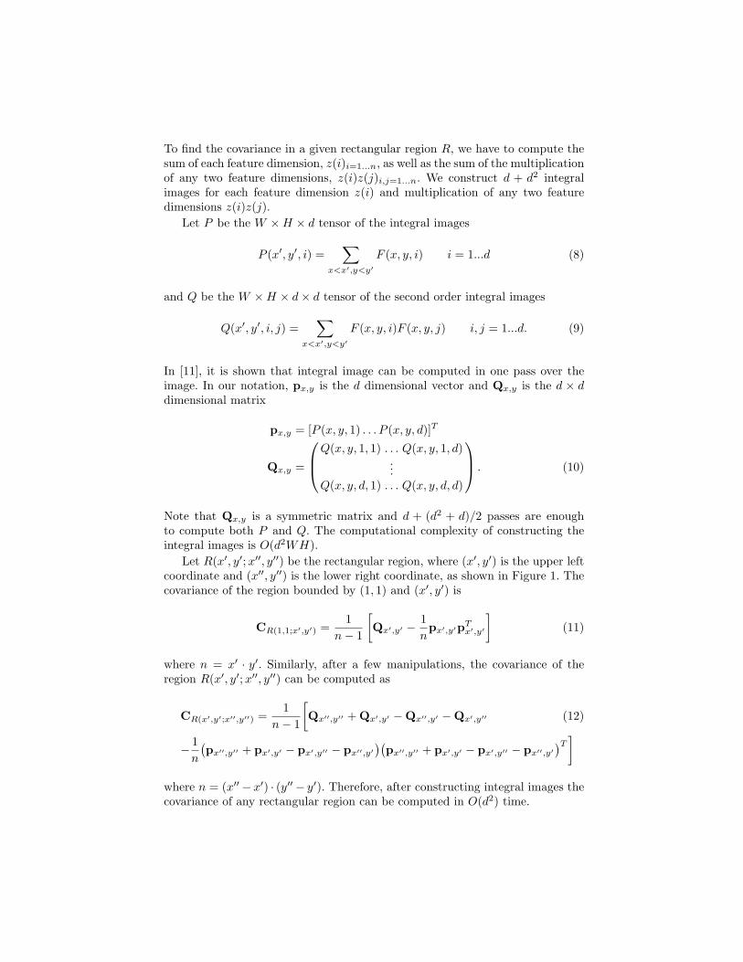
To find the covariance in a given rectangular region R, we have to compute thesum of each feature dimension, z(i)i=1...n, as well as the sum of the multiplicationof any two feature dimensions, z(i)z(j)i,j=1...n. We construct d + d2 integralimages for each feature dimension z(i) and multiplication of any two featuredimensions z(i)z(j).

Let P be the W ×H × d tensor of the integral images

P (x′, y′, i) =∑

x<x′,y<y′

F (x, y, i) i = 1...d (8)

and Q be the W ×H × d× d tensor of the second order integral images

Q(x′, y′, i, j) =∑

x<x′,y<y′

F (x, y, i)F (x, y, j) i, j = 1...d. (9)

In [11], it is shown that integral image can be computed in one pass over theimage. In our notation, px,y is the d dimensional vector and Qx,y is the d × ddimensional matrix

px,y = [P (x, y, 1) . . . P (x, y, d)]T

Qx,y =

Q(x, y, 1, 1) . . . Q(x, y, 1, d)...

Q(x, y, d, 1) . . . Q(x, y, d, d)

. (10)

Note that Qx,y is a symmetric matrix and d + (d2 + d)/2 passes are enoughto compute both P and Q. The computational complexity of constructing theintegral images is O(d2WH).

Let R(x′, y′;x′′, y′′) be the rectangular region, where (x′, y′) is the upper leftcoordinate and (x′′, y′′) is the lower right coordinate, as shown in Figure 1. Thecovariance of the region bounded by (1, 1) and (x′, y′) is

CR(1,1;x′,y′) =1

n− 1

[Qx′,y′ − 1

npx′,y′pT

x′,y′

](11)

where n = x′ · y′. Similarly, after a few manipulations, the covariance of theregion R(x′, y′;x′′, y′′) can be computed as

CR(x′,y′;x′′,y′′) =1

n− 1

[Qx′′,y′′ + Qx′,y′ −Qx′′,y′ −Qx′,y′′ (12)

− 1n

(px′′,y′′ + px′,y′ − px′,y′′ − px′′,y′

)(px′′,y′′ + px′,y′ − px′,y′′ − px′′,y′

)T]

where n = (x′′ − x′) · (y′′ − y′). Therefore, after constructing integral images thecovariance of any rectangular region can be computed in O(d2) time.

Fig. 2. Object representation. We construct five covariance matrices from overlappingregions of an object feature image. The covariances are used as the object descriptors.

3 Object Detection

In object detection, given an object image, the aim is to locate the object in anarbitrary image and pose after a nonrigid transformation. We use pixel locations(x,y), color (RGB) values and the norm of the first and second order derivativesof the intensities with respect to x and y. Each pixel of the image is convertedto a nine-dimensional feature vector

F (x, y) =

[x y R(x, y) G(x, y) B(x, y)

∣∣∣∣∂I(x, y)∂x

∣∣∣∣ ∣∣∣∣∂I(x, y)∂y

∣∣∣∣ ∣∣∣∣∂2I(x, y)∂x2

∣∣∣∣ ∣∣∣∣∂2I(x, y)∂y2

∣∣∣∣]T

(13)

where R, G, B are the RGB color values, and I is the intensity. The imagederivatives are calculated through the filters [−1 0 1]T and [−1 2 − 1]T . Thecovariance of a region is a 9× 9 matrix. Although the variance of pixel locations(x,y) is same for all the regions of the same size, they are still important sincetheir correlation with the other features are used at the nondiagonal entries ofthe covariance matrix.

We represent an object with five covariance matrices of the image featurescomputed inside the object region, as shown in Figure 2. Initially we computeonly the covariance of the whole region, C1, from the source image. We search thetarget image for a region having similar covariance matrix and the dissimilarity ismeasured through (3). At all the locations in the target image we analyze at ninedifferent scales (four smaller, four larger) to find matching regions. We performa brute force search, since we can compute the covariance of an arbitrary regionvery quickly. Instead of scaling the target image, we just change the size of oursearch window. There is a 15% scaling factor between two consecutive scales. Thevariance of the x and y components are not the same for regions with differentsizes and we normalize the rows and columns corresponding to these features. Atthe smallest size of the window we jump three pixels horizontally or verticallybetween two search locations. For larger windows we jump 15% more and roundto the next integer at each scale.

We keep the best matching 1000 locations and scales. At the second phasewe repeat the search for 1000 detected locations, using the covariance matricesCi=1...5. The dissimilarity of the object model and a target region is computed

ρ(O, T ) = minj

[5∑

i=1

ρ(COi ,CT

i )− ρ(COj ,CT

j )

](14)

where COi and CT

i are the object and target covariances respectively, and weignore the least matching region covariance of the five. This increases robustnesstowards possible occlusions and large illumination changes. The region with thesmallest dissimilarity is selected as the matching region.

We present the matching results for a variety of examples in Figure 3 andcompare our results with histogram features. We tested histogram features bothwith the RGB and HSV color spaces. With the RGB color space the resultswere much worse in all of the cases, therefore we did not present these results.We construct three separate 64 bin histograms for hue, saturation and valuesince it is not practical to construct a joint histogram. We search the targetimage for the same locations and sizes, and fast construction of histograms areperformed through integral histograms [7]. We measure the distance betweentwo histograms through Bhattacharyya distance [6] and sum over three colorchannels.

Covariance features can match all the target regions accurately whereas mostof the regions found by histogram are erroneous. Even among the correctly de-tected regions with both methods we see that covariance features better localizethe target. The examples are challenging since there are large scale, orienta-tion and illumination changes, and some of the targets are occluded and havenonrigid motion. Almost perfect results indicate the robustness of the proposedapproach. We also conclude that the covariances are very discriminative sincethey can match the correct target in the presence of similar objects, as seen inthe face matching examples.

Covariance features are faster than the integral histograms since the dimen-sionality of the space is smaller. The search time of an object in a color imagewith size 320× 240 is 6.5 seconds with a MATLAB 7 implementation. The per-formance can be improved by a factor of 20-30 with a C++ implementationwhich would yield to near real time performance.

4 Texture Classification

Currently, the most successful methods for texture classification are throughtextons which are cluster centers in a feature space derived from the input. Thefeature space is built from the output of a filter bank applied at every pixel andthe methods differ only in the employed filter bank.

– LM: A combination of 48 anisotropic and isotropic filters were used by Leungand Malik [8]. The feature space is 48 dimensional.

(a) (b) (c)

Fig. 3. Object detection. (a) Input regions. (b) Regions found via covariance features.(c) Regions found via histogram features.

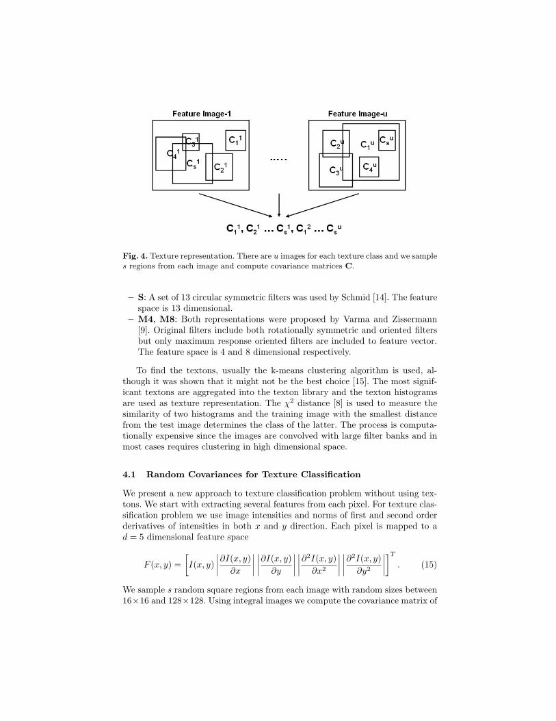
Fig. 4. Texture representation. There are u images for each texture class and we samples regions from each image and compute covariance matrices C.

– S: A set of 13 circular symmetric filters was used by Schmid [14]. The featurespace is 13 dimensional.

– M4, M8: Both representations were proposed by Varma and Zissermann[9]. Original filters include both rotationally symmetric and oriented filtersbut only maximum response oriented filters are included to feature vector.The feature space is 4 and 8 dimensional respectively.

To find the textons, usually the k-means clustering algorithm is used, al-though it was shown that it might not be the best choice [15]. The most signif-icant textons are aggregated into the texton library and the texton histogramsare used as texture representation. The χ2 distance [8] is used to measure thesimilarity of two histograms and the training image with the smallest distancefrom the test image determines the class of the latter. The process is computa-tionally expensive since the images are convolved with large filter banks and inmost cases requires clustering in high dimensional space.

4.1 Random Covariances for Texture Classification

We present a new approach to texture classification problem without using tex-tons. We start with extracting several features from each pixel. For texture clas-sification problem we use image intensities and norms of first and second orderderivatives of intensities in both x and y direction. Each pixel is mapped to ad = 5 dimensional feature space

F (x, y) =[I(x, y)

∣∣∣∣∂I(x, y)∂x

∣∣∣∣ ∣∣∣∣∂I(x, y)∂y

∣∣∣∣ ∣∣∣∣∂2I(x, y)∂x2

∣∣∣∣ ∣∣∣∣∂2I(x, y)∂y2

∣∣∣∣]T

. (15)

We sample s random square regions from each image with random sizes between16×16 and 128×128. Using integral images we compute the covariance matrix of

each region. Each texture image is then represented with s covariance matricesand we have u training texture images from each texture class, a total of s · ucovariance matrices. Texture representation process is illustrated in Figure 4.We repeat the process for the c texture classes and construct the representationfor each texture class in the same way.

Given a test image, we again extract s covariance matrices from randomlyselected regions. For each covariance matrix we measure the distance (3) fromall the matrices of the training set and the label is predicted according to themajority voting among the k nearest ones (kNN algorithm). This classifier per-forms as a weak classifier and the class of the texture is determined accordingto the maximum votes among the s weak classifiers.

4.2 Texture Classification Experiments

We perform our tests on the Brodatz texture database which consists of 112textures. Because of the nonhomogeneous textures inside the database, classi-fication is a challenging task. We duplicate the test environment of [15]. Each640× 640 texture image is divided into four 320× 320 subimages and half of theimages are used for training and half for testing.

We compare our results with the results reported in [15] in Table 1. Here wepresent the results for k-means based clustering algorithm. The texture repre-sentation through texton histograms has 560 bins. The results vary from 85.71%to 97.32% depending on the filter bank used.

In our tests we sample s = 100 random covariances from each image, bothfor testing and training, and we used k = 5 for the kNN algorithm. For d = 5dimensional features, the covariance matrix is 5 × 5 and has only 15 differentvalues compared to 560 bins before. Our result, 97.77%, is better than all of theprevious results and faster. Only 5 images out of 224 is misclassified which isclose to the upper limit of the problem. We show two of the misclassified imagesin Figure 5 and the misclassification is usually in nonhomogeneous textures.

To make the method rotationally invariant, we used only three rotationallyinvariant features: intensity and the magnitude of the gradient and Laplacian.The covariance matrices are 3 × 3 and have only 6 different values. Even withthis very simple features the classification performance is 94.20%, which is asgood as or even better than other rotationally invariant methods (M4, M8, S)listed in Table 1. Due to random sized window selection our method is scaleinvariant. Although the approach is not completely illumination invariant, it ismore robust than using features (intensity and gradients) directly. The variancesof intensity and gradients inside regions change less than intensity and gradientsthemselves in illumination variations.

M4 M8 S LM Random Covariance

Performance 85.71 94.64 93.30 97.32 97.77

Table 1. Classification results for the Brodatz database.

(a) (b) (c)

Fig. 5. Misclassified samples. (a) Test examples. (b) Samples from the same class. (c)Samples from the predicted texture class.

Raw Inten. Inten. Hist. Inten./Deriv. Hist. Covariance

Performance 26.79 83.35 96.88 97.77

Table 2. Classification results for different features.

In the second experiment we compare the covariance features with otherpossible choices. We run the proposed texture classification algorithm with theraw intensity values and histograms extracted from random regions.

For raw intensities we normalize each random region to 16×16 square regionand use Euclidean distance to compute distances for kNN classification, whichis similar to [3]. The feature space is 256 dimensional. The raw intensity valuesare very noisy therefore only in this case we sample s = 500 regions from eachimage.

We perform two tests using histogram features: intensity only, and inten-sity and norms of first and second order derivatives together. In both cases thedissimilarity is measured with Bhattacharyya distance [6]. We use 256 bins forintensity only and 5 · 64 = 320 bins for intensity and norm of derivatives to-gether. It is not practical to construct the joint intensity and norm of derivativeshistograms, due to computational and memory requirement.

We sample s = 100 regions from each texture image. The results are shownin Table 2. The only result close to covariance is the 320 dimensional intensityand derivative histograms together. This is not surprising because our covari-ance features are the covariances of the joint distribution of the intensity andderivatives. But with covariance features we achieve a better performance in amuch faster way.

5 Conclusion

In this paper we presented the covariance features and related algorithms for ob-ject detection and texture classification. Superior performance of the covariance

features and algorithms were demonstrated on several examples with detailedcomparisons to previous techniques and features. The method can be extendedin several ways. For example, following automatical detection of an object ina video, it can be tracked in the following frames using this approach. As theobject leaves the scene, the distance score will increase significantly which endsthe tracking. Currently we are working on classification algorithms which usethe Lie group structure of covariance matrices.

References

1. Rosenfeld, A., Vanderburg, G.: Coarse-fine template matching. IEEE Trans. Syst.Man. Cyb. 7 (1977) 104–107

2. Brunelli, R., Poggio, T.: Face recognition: Features versus templates. IEEE Trans.Pattern Anal. Machine Intell. 15 (1993) 1042 – 1052

3. Maree, R., Geurts, P., Piater, J., Wehenkel, L.: Random subwindows for robustimage classification. In: Proc. IEEE Conf. on Computer Vision and Pattern Recog-nition, San Diego, CA. Volume 1. (2005) 34–40

4. Turk, M., Pentland, A.: Face recognition using eigenfaces. In: Proc. IEEE Conf.on Computer Vision and Pattern Recognition, Maui, HI. (1991) 586–591

5. Black, M., Jepson, A.: Eigentracking: Robust matching and tracking of articulatedobjects using a view-based representation. Intl. J. of Comp. Vision 26 (1998) 63–84

6. Comaniciu, D., Ramesh, V., Meer, P.: Real-time tracking of non-rigid objects usingmean shift. In: Proc. IEEE Conf. on Computer Vision and Pattern Recognition,Hilton Head, SC. Volume 1. (2000) 142–149

7. Porikli, F.: Integral histogram: A fast way to extract histograms in cartesian spaces.In: Proc. IEEE Conf. on Computer Vision and Pattern Recognition, San Diego,CA. Volume 1. (2005) 829 – 836

8. Leung, T., Malik, J.: Representing and recognizing the visual appearance of ma-terials using three-dimensional textons. Intl. J. of Comp. Vision 43 (2001) 29–44

9. Varma, M., Zisserman, A.: Statistical approaches to material classification. In:Proc. European Conf. on Computer Vision, Copehagen, Denmark. (2002)

10. Georgescu, B., Meer, P.: Point matching under large image deformations andillumination changes. IEEE Trans. Pattern Anal. Machine Intell. 26 (2004) 674–688

11. Viola, P., Jones, M.: Rapid object detection using a boosted cascade of simplefeatures. In: Proc. IEEE Conf. on Computer Vision and Pattern Recognition,Kauai, HI. Volume 1. (2001) 511–518

12. Lowe, D.: Distinctive image features from scale-invariant keypoints. Intl. J. ofComp. Vision 60 (2004) 91–110

13. Forstner, W., Moonen, B.: A metric for covariance matrices. Technical report,Dept. of Geodesy and Geoinformatics, Stuttgart University (1999)

14. Schmid, C.: Constructing models for content-based image retreival. In: Proc. IEEEConf. on Computer Vision and Pattern Recognition, Kauai, HI. (2001) 39–45

15. Georgescu, B., Shimshoni, I., Meer, P.: Mean shift based clustering in high di-mensions: A texture classification example. In: Proc. 9th Intl. Conf. on ComputerVision, Nice, France. (2003) 456–463