Embed Size (px)
Citation preview

I
Mechatronikai modellezés Dr. Szabó Tamás
Copyright © 2014 Miskolci Egyetem
A tananyag a TÁMOP-4.1.2.A/1-11/1-2011-0042 azonosító számú „ Mechatronikai mérnök MSc tananyagfejlesztés ” projekt keretében készült. A tananyagfejlesztés az Európai Unió támogatásával és az Európai Szociális Alap társfinanszírozásával valósult meg.
Kézirat lezárva: 2014 február
A kiadásért felel a(z): Miskolci Egyetem
Felelős szerkesztő: Miskolci Egyetem
2014

Mechatronical Modelling

CONTENTS III
Table of Contents
1 Introduction 1
1.1 Introductive Examples.................................................................................................. 2
1.2 The Dynamical System ................................................................................................. 4
1.2.1 Definitions ...................................................................................................... 5
1.2.2 System Classification .................................................................................... 10
1.3 System Models ........................................................................................................... 11
1.3.1 Model Types ................................................................................................. 11
1.3.2 System Analysis ............................................................................................ 12
1.3.3 System Simulation ........................................................................................ 13
1.3.4 System Identification ................................................................................... 14
1.3.5 System Optimization (cp. Chapter 10) ......................................................... 15
1.3.6 Model Schemes and Block Diagrams ........................................................... 16
1.4 Task of System Dynamics ........................................................................................... 20
1.5 Summary .................................................................................................................... 22
2 Mathematical Description of Dynamical Systems 24
2.1 Differential Equations ................................................................................................ 24
2.2 State Equations .......................................................................................................... 28
2.3 Stationary Solutions and Equilibrium Positions ......................................................... 31
2.4 Linear State Equations ............................................................................................... 33
2.5 Analysis of Typical Problems of System Dynamics by Means of State Equations ..... 39
3 Differential-Algebraic-Equation-Systems and Multiport Method 42
3.1 Differential-Algebraic-Equation-Systems (DAE-Systems) .......................................... 42
3.2 The “Cut-Set“ or “Multiport“-Method ....................................................................... 47
3.2.1 Basic Idea ..................................................................................................... 47
3.2.2 Equation Structure ....................................................................................... 49
3.2.3 Examples ...................................................................................................... 52
4 Solution of State Space Equations 61
4.1 Existence and Uniqueness of Solutions of Ordinary Differential Equations .............. 61
4.2 Solution Design in the Phase Plane ............................................................................ 64
4.3 Solution Methods for Linear State Equations ............................................................ 66
4.3.1 Solution of homogenous Systems, Fundamental Matrix ............................ 66
4.3.2 Solution of the inhomogeneous State Equation .......................................... 70
5 State Space Equations with Normal Coordinates 73
5.1 Normal Coordinates ................................................................................................... 73
5.2 Eigenbehaviour of Systems with Multiple Eigenvalues ............................................. 83
5.2.1 Effect of Multiple Eigenvalues ..................................................................... 83
5.2.2 Jordan’s Normal Form .................................................................................. 85
6 Numerical Methods with Dynamical Systems 91
6.1 Introduction ............................................................................................................... 91
6.1.1 Taylor Expansion .......................................................................................... 91
6.1.2 Numerical Algorithms .................................................................................. 92
6.1.3 Rounding Error and Error Propagation ........................................................ 93
7 Numerical Methods for Initial Value Problems 97
7.1 Numerical Solution of Initial Value Problems ............................................................ 97
7.1.1 Explicit Euler Method (Forward Euler Method) ........................................... 97
7.1.2 Numerical Stability and Stability Domain .................................................. 101
7.1.3 Modified Euler Method (Trapezoidal Rule) ............................................... 102
7.1.4 Implicit Euler method ................................................................................ 106
7.1.5 Summary of Euler’s Method ...................................................................... 107
7.1.6 General One-Step Procedures ................................................................... 107
7.1.7 Step Size Control ........................................................................................ 115
7.1.8 Linear Multi-Step Methods ........................................................................ 118
7.1.9 Activation of Linear Multi-Step Procedures ............................................... 122
7.1.10 System of Differential Equations ............................................................... 123
7.1.11 BDF Methods .............................................................................................. 123
7.1.12 Remarks on Stiff Differential Equations ..................................................... 125
7.1.13 Implicit Runge-Kutta Methods ................................................................... 133
7.1.14 Comparison of Methods for Numerical Solution of Initial Value Problems (IVP) ............................................................................................................ 135
8 Integration of Discontinuous Systems and DAEs 137
8.1 Integration of Discontinuous Systems ..................................................................... 137
8.2 Differential Algebraic Equations (DAEs) ................................................................... 138
9 Numerical Solution of Non-linear Sysem Equations 143
9.1 Nonlinear Equations ................................................................................................. 143
9.2 Solution with Numerical Integration........................................................................ 147
9.3 Fixed Point Iteration ................................................................................................. 148
9.4 Newton-Raphson Iteration ...................................................................................... 150
10 Identification and Optimisation 153
10.1 Linear Compensation Problem ................................................................................. 154
10.2 Non-linear Parameter Dependency ......................................................................... 157
10.3 Stability of Dynamical Systems ................................................................................ 159
10.4 Stability Criteria for Linear Systems ......................................................................... 161
10.4.1 Stability Criteria based on Stodola ............................................................. 161
10.4.2 Hurwitz Criteria .......................................................................................... 162
10.4.3 Stability Criteria based on Routh ............................................................... 164

CONTENTS V
11 Modelling of Mechanical Systems 167
11.1 Fundamental Terms ................................................................................................. 167
11.1.1 Modelling: Mass, Elasticity and Damping .................................................. 167
11.1.2 Forces, System Boundary, Method of Sections ......................................... 169
11.1.3 Constraints ................................................................................................. 170
11.1.4 Virtual Displacements ................................................................................ 171
11.1.5 Kinematics .................................................................................................. 173
11.2 Principle of Linear and Angular Momentum ............................................................ 179
11.3 Consideration of Constraints and the Principle of d’Alembert................................ 180
11.4 Equations of Motion ................................................................................................ 181
11.5 Equations of Motion of a Double Pendulum ........................................................... 181
11.6 Linear Equations of Motion ...................................................................................... 186
11.7 State Equations ........................................................................................................ 189
12 Lagrange’s Equations of Motion of Second Kind 191
13 Nonlinear Single Track Modell (based on [9] 196
13.1 Equations of Motion of the chassis .......................................................................... 197
13.2 Tyre Model ............................................................................................................... 198
13.2.1 Stationary Tyre Model ............................................................................... 198
13.2.2 Dynamic Tyre Model .................................................................................. 201
14 Dynamic Wheel Rotation 203
14.1 Driving Torques ........................................................................................................ 203
14.2 Breaking Torques ..................................................................................................... 204
15 The Overall Modell 205
15.1 Simulation Results .................................................................................................... 207
15.2 Animations ............................................................................................................... 208
15.3 Videos ....................................................................................................................... 209
16 Mathematical Basics 211
16.1 Matrix Calculations .................................................................................................. 211
16.1.1 Matrix Operations ...................................................................................... 213
16.1.2 Determinants ............................................................................................. 218
16.1.3 Norms ......................................................................................................... 219
17 Worksheets 221
18 Exercises 237
19 References 240

List of Figures Fig. 1.1: System descriptions in different fields of study [1]. .................................................................. 1 Fig. 1.2: ABS- magnetic valves, interfaces. .............................................................................................. 3 Fig. 1.3: Above: Percussion hammer [2]; Below: Simulation model of a percussion hammer. .............. 4 Fig. 1.4: Representation of a system as a block. ..................................................................................... 6 Fig. 1.5: System of a motor vehicle [5]. ................................................................................................... 7 Fig. 1.6: Degrees of freedom of the spatial twin-track model [6]. .......................................................... 8 Fig. 1.7: Principle process of system simulation.................................................................................... 13 Fig. 1.8: Process of parameter identification. ....................................................................................... 15 Fig. 1.9: Process of system optimization. .............................................................................................. 16 Fig. 1.10: Example of a block diagram (single mass pendulum). ........................................................... 17 Fig. 1.11: Simple model of a wheel suspension. ................................................................................... 18 Fig. 1.12: Block diagram for suspension, possible refinement levels. ................................................... 19 Fig. 1.13: Electrical low pass-filter. ........................................................................................................ 19 Fig. 1.14: Block diagram for electrical low-pass filter, possible refinement levels. .............................. 20 Fig. 1.15: Signal flow diagrams for a) suspension and b) low-pass filter............................................... 20 Fig. 2.1: Mathematical pendulum. ........................................................................................................ 24 Fig. 2.2: Longitudinal beam oscillations. ............................................................................................... 25 Fig. 2.3: Discrete model of the description of longitudinal oscillations. ............................................... 26 Fig. 2.4: Simple frequency response system with concentrated parameters (multybody system). ..... 28 Fig. 2.5: Block diagram of the non-linear state equation. ..................................................................... 29 Fig. 2.6: Block diagram: Logistical growth at constant crop. ................................................................. 31 Fig. 2.7: Linearisation of a scalar function of a variable. ....................................................................... 33 Fig. 2.8: Block diagram of additivity of a linear relation. ....................................................................... 35 Fig. 2.9: Non-linear force characteristic (in combination with play). .................................................... 35 Fig. 2.10: Block diagram of linear state equations. ............................................................................... 38 Fig. 3.1: Non-linear simple pendulum. .................................................................................................. 43 Fig. 3.2: Simulation on the basis of state equations. ............................................................................ 47 Fig. 3.3: Object-oriented modelling/simulation. ................................................................................... 47 Fig. 3.4: Block diagram. ......................................................................................................................... 48 Fig. 3.5: Difference measurement (across). .......................................................................................... 48 Fig. 3.6: Flow measurement (through). ................................................................................................. 48 Fig. 3.7: Linkage of objects on the basis of the Cut-Set method. .......................................................... 49 Fig. 3.8: Mathematical pendulum example. .......................................................................................... 50 Fig. 3.9: Graphical representation. ........................................................................................................ 51 Fig. 3.10: Sign convention. .................................................................................................................... 51 Fig. 3.11: Ohmic resistance. .................................................................................................................. 52 Fig. 3.12: Inductive reactance. .............................................................................................................. 52 Fig. 3.13: Capacity.................................................................................................................................. 53 Fig. 3.14: Simple electrical network. ..................................................................................................... 53 Fig. 3.15: Spring. .................................................................................................................................... 55 Fig. 3.16: Multiport model spring. ......................................................................................................... 56 Fig. 3.17: Mass. ...................................................................................................................................... 56 Fig. 3.18: Multiport model mass ........................................................................................................... 56 Fig. 3.19: Spring-mass system. .............................................................................................................. 57 Fig. 3.20: Multiport. ............................................................................................................................... 58 Fig. 4.1: Solution of the equation for logistic growth (qualitative). ...................................................... 64 Fig. 4.2: Phase curves of the mathematical pendulum. ........................................................................ 66 Fig. 5.1: Decaying behaviour with real eigenvalues. ............................................................................. 78 Fig. 5.2: Decaying behaviour with complex eigenvalues. ...................................................................... 79 Fig. 5.3: Behaviour of linear systems in dependence of the position of the complex plane. ............... 80

7
Fig. 5.4: Quarter-car. ............................................................................................................................. 80 Fig. 5.5: Eigenvalues of the quarter-car where 1500 Ns/m ≤ dA ≤ 6500 Ns/m...................................... 83 Fig. 7.1: Forward Euler Method. ............................................................................................................ 98 Fig. 7.2: Application of forward Euler method. ................................................................................... 100 Fig. 7.3: Forward Euler method; instability. ........................................................................................ 100 Fig. 7.4: Stability domain of the explicit Euler’s method. .................................................................... 102 Fig. 7.5: Derivation of the Trapezoidal Rule. ....................................................................................... 103 Fig. 7.6: Stability domain after applying the fixed-point iteration. ..................................................... 105 Fig. 7.7: The implicit Euler method...................................................................................................... 107 Fig. 7.8: Instability area in the Runga-Kutta method of 4th order. ...................................................... 112 Fig. 7.9: Transition points in the Runge-Kutta method. ...................................................................... 113 Fig. 7.10: Stability area of the Runge-Kutta method of order 1-4. ...................................................... 115 Fig. 7.11: Step size control depicted as a (feedback) control problem ............................................... 118 Fig. 7.12: Integration of one-mass pendulum by means of the explicit Euler method. ...................... 128 Fig. 7.13: Integration of one-mass oscillator by means of the implicit Euler method. ....................... 131 Fig. 7.14: Energy behaviour of a plane oscillator. ............................................................................... 132 Fig. 7.15: A(0)-stability. ........................................................................................................................ 133 Fig. 8.1: Bouncing ball. ......................................................................................................................... 137 Fig. 8.2: Bouncing ball (simulation result). .......................................................................................... 138 Fig. 9.1: Planar fourbar mechanism. ................................................................................................... 144 Fig. 9.2: Solutions of the planar four-bar mechanism. ........................................................................ 145 Fig. 9.3: Five-link wheel suspension. ................................................................................................... 145 Fig. 9.4: Vectors of the five-point wheel suspension. ......................................................................... 147 Fig. 9.5: Wheel centre trajectory of the five-point real axle wheel suspension. ................................ 147 Fig. 9.6: Convergent fix-point iteration; gradient in fix point. ............................................................ 149 Fig. 9.7: Divergent fix point iteration .................................................................................................. 150 Fig. 9.8: Newton-Raphson iteration steps. .......................................................................................... 151 Fig. 10.1: Parameter determined system. ........................................................................................... 153 Fig. 10.2: Target system....................................................................................................................... 156 Fig. 10.3: Geometric illustration of the pseudoinverse. ...................................................................... 157 Fig. 10.4: Simulator model .................................................................................................................. 157 Fig. 10.5: Scan of y(t) ........................................................................................................................... 158 Fig. 11.1: Examples for elements of a multi-body system. ................................................................. 169 Fig. 11.2: Method of section in mechanics. ......................................................................................... 170 Fig. 11.3: Examples for constraints...................................................................................................... 171 Fig. 11.4: Sphere pendulum. ............................................................................................................... 173 Fig. 11.5: Virtual Displacement. .......................................................................................................... 173 Fig. 11.6: Coordinate transformation by rotation around the z-axis. ................................................. 175 Fig. 11.7: Double pendulum. ............................................................................................................... 182 Fig. 13.1: Nonlinear single track model (bicycle model), top view ..................................................... 196 Fig. 13.2: Nonlinear single track model, side view .............................................................................. 196 Fig. 14.1: Dynamic wheel rotation. ..................................................................................................... 203 Fig. 14.2: Engine characteristics. ......................................................................................................... 204 Fig. 14.3: Braking torque characteristics. ............................................................................................ 205 Fig. 15.1: Nonlinear single track model: different steering wheel angle jumps at v = 100km/h. ....... 208
List of Tables Table 1.1: Examples of state variables in different disciplines. .............................................................. 7 Table 1.2: Examples of system elements from different disciplines. ...................................................... 8 Table 3.1: Classification of across and through qualities in various fields. ........................................... 48 Table 7.1: Accumulation of the amount of transition values and achieved order. ............................ 114 Table 7.2: Opening angle α for different k .......................................................................................... 133


1
1 Introduction
This manuscript contains descriptions of modelling and simulation methods and aims at
understanding the characteristics of complex (and other) dynamical systems in order to
influence them effectively.
Consequently, it is required to know how to apply methods of modelling and analysis of such
systems, their subsystems and components reasonably. This lecture deals with:
• mathematical formulations of dynamical systems,
• modelling techniques,
• simulation,
• numerical methods to integrate differential equations and to solve non-linear equation systems,
• identification and estimation of system parameters,
• stabilizing characteristics of dynamical systems.
In this context it is important to emphasize that the subject systems are not part of one particular discipline (e.g. mechanics), but that in order to describe such systems academic
collaborations between different methods of branches of study have to be made, cp. Fig.
1.1.
Fig. 1.1: System descriptions in different fields of study [1].

2
1.1 Introductive Examples
The following examples will be covered in lecture in more detail.
Example 1.1: ABS – Magnetic Valve, Fig. 1.2
System: ABS
Subsystem (components): Magnetic valve
Potential objectives:
a) Describe the time-dependent process x(t) of the armature .
b) Where and how one can exert influence on the dynamic behaviour (e.g. a faster build-
up of x to 90% of the total travel)?
c) What other objectives of non-dynamic nature exist in this context? d) What other opportunities exist to influence the dynamic characteristics in a positive
way (what is the meaning of “positive” in this context?)?
The construction of the ABS involves different disciplines of engineering, e.g.:
• mechanics (brake mechanism, driving dynamics),
• hydraulics (valves, pumps, pipes, ...),
• electrotechnology (controller, power electronics, …),
• control theory (ABS-algorithm).

3
Fig. 1.2: ABS- magnetic valves, interfaces.
Example 1.2: Percussion Hammer, Fig. 1.3
System: Percussion hammer
Subsystem (component): Crank mechanism
Potential objectives:
a) Maximize the impulse velocity of the percussion.
b) Minimize the vibrations of the hand grip while keeping the percussion power at a
constant level. c) How must the components of the crank mechanism be designed in order to achieve
good results of drilling?
d) Is there a potential risk of breakage caused by heavy dynamic (working voltage)
loadings on the components of the crank mechanism?

4
Fig. 1.3: Above: Percussion hammer [2]; Below: Simulation model of a percussion hammer.
Worksheet 1: Simple simulation model of a percussion hammer [3]
1.2 The Dynamical System
Examples of the colloquial usage of the term system are solar system, transportation system,
computer system, cardiovascular system, nervous system, etc.
In this context and in the fields of engineering and science, the term system is used in
connection with complex and in transparent operations and processes. In general, we can observe a collaboration of different disciplines.

5
1.2.1 Definitions
Definition 1.1 [3]:
A system is a set of elements (parts, components, objects),
• Which mutually influence each other (interaction),
• Which are subjected to external influences and affection (input) and
• Which effect to the external (output).
Annotation 1.1:
Science provides access to various definitions of the term system, e.g.:
Definition 1.2 [4]:
An object is identified as a system as long as all particular elements and all attributes with
their interdependencies (to outside the system also) are seen to be components of that whole in some logical sense. Additionally, there are axioms.
Elements are e.g. modules, components, objects, fractions.
Attributes are properties, qualities, features, characteristics and also interfaces between the
system and its environment. The term state characterizes the constitution of the system at any given time.
Definition 1.3 [4]:
A system is a well-defined assembly which consists of interacting entities. This assembly is
delimited by a cladding plain or boundary (a set of system elements with interfaces to
outside the system). The cladding plain provides for an interface between the system and its
environment. The relationships between attributes and states, transported by the interfaces
mentioned above, are variables which describe the peculiar characteristics of the system.
A block is a way of illustrating a system. The borderline represents the cladding plain.

6
Fig. 1.4: Representation of a system as a block.
Interfaces are
• r input quantities iu ,
• m output quantities iy and
• q interfering quantities iz , if applicable.
Closed systems are self-contained and maintain no connections with the environment, i.e.
outside events have no influence on the system. The total state of the system is defined by n
state quantities ix .
Definition 1.4:
State variables are those variables in a system, which completely describe the system’s
behaviour. State variables are time-dependent. The term system state refers to the entirety
of all values of the state variables.
Annotation 1.2:
• State variables are “internal variables” of a system.
• There is no definite choice of state variables. But characteristics can be assigned to the
chosen state variables, such as uniqueness, independence and freedom of redundancy.
From the latter characteristic it follows that the choice of state variables is absolutely
arbitrary; however, the values are fixed.
• In practice, one is not interested in the entirety of all state variables, but only chooses
the variables needed for the application; the so-called output quantities. Output quantities can also result from a combination of state variables.
Examples of state variables from different disciplines; cp Table 1.1.
7
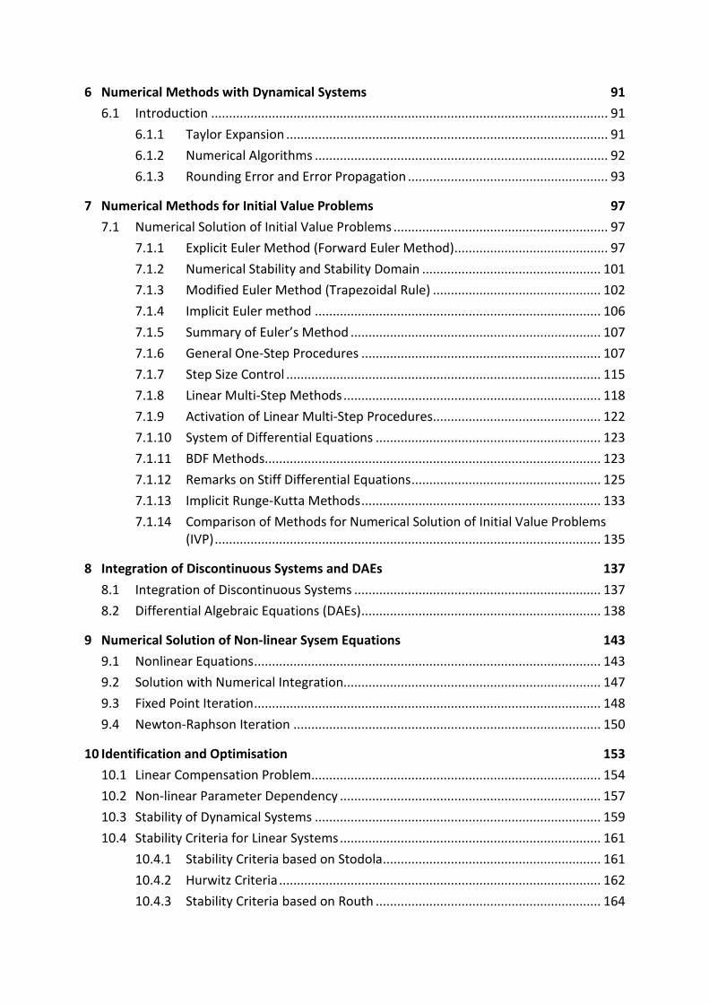
Table 1.1: Examples of state variables in different disciplines.
Electrotechnology Mechanics Process engineering Environmental engineering
Current Position Temperature Population
Voltage Velocity Mass fraction Environmental state
Load Acceleration CO2 production
Kinetic energy Ozone value
Potential energy
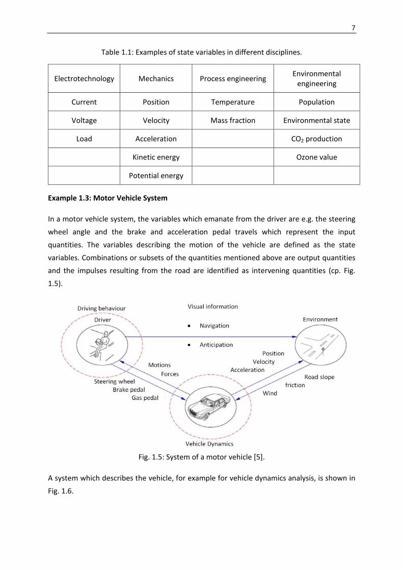
Example 1.3: Motor Vehicle System
In a motor vehicle system, the variables which emanate from the driver are e.g. the steering
wheel angle and the brake and acceleration pedal travels which represent the input
quantities. The variables describing the motion of the vehicle are defined as the state
variables. Combinations or subsets of the quantities mentioned above are output quantities and the impulses resulting from the road are identified as intervening quantities (cp. Fig.
1.5).
Fig. 1.5: System of a motor vehicle [5].
A system which describes the vehicle, for example for vehicle dynamics analysis, is shown in
Fig. 1.6.

8
Fig. 1.6: Degrees of freedom of the spatial twin-track model [6].
Example 1.4: Framework System
Elements of the system are specific bars of the framework. Internal interactions between the
bars are nodal forces. Input quantities are external loads and reaction forces in the bearings
can be defined as output quantities.
Example 1.5: Road Traffic System
Specific motor vehicles are the system elements in a delimited road traffic network. The
driver and his motor vehicle can represent the subsystems. Internal interactions can be comparative distances and relative velocities of the vehicles to each other.
Definition 1.5:
A system with more than one input quantity and more than one output quantity is defined
as a multi-quantities system (multi-input-multi-output system “MIMO”).
System elements from different technical disciplines are listed in Table 1.2.
Table 1.2: Examples of system elements from different disciplines.
Electrotechnology Mechanics Process engineering Population development
Resistance Mass Vessel Birth
Capacitor Spring Valve Death
Coil Damper Pipe line Disease

9
Transistor Beam Stirrer vessel Consumption
Amplifier Bearing Filter
Filter Guidance Reactor
Dead stop
Position actuator
Force actuator
The form of interaction between the system elements defines the system structure. A
system can be structured into subsystems (components).
The structuring process into subsystems has the advantage that we obtain a better overview of the behaviour of the system and that the subsystems can be constructed by different
people. The structuring process should be carried out in such way that the subsystems can
be reintegrated into the total system. This makes the clear definition of the interfaces inevitable, which also represents one of the major problems of industrial treatment of
complex dynamical systems.
The system boundary (cladding plain) is arbitrary. But in general, limitations are introduced
where a clear distinction to the environment exists, with a few uniquely defined relationships that can be observed and where the system is reactionless to its environment.
Definition 1.6:
The motion of dynamical systems is a change of the variables of the system with respect to
time. Mechanical motion (changes referring to place) represents a special case of all general
types of motions.
Furthermore, the term motion appears in literature a number of times, [7]:
System parameters are quantities which remain constant for the system during the
observation period. Examples are given by natural constants, spring constants and damping
factors, resistance, etc.
Environmental influences are quantities which affect the system from the outside, but which
are not influenced by the system in return (reactionless). Examples are changes in
temperature in big rooms, forced movements, etc.

10
Initial values of the state quantities.
Rate of change of a state quantity refers to the rate at which the value of the state quantity
changes in course of time. Examples are given by velocity, acceleration, rate of birth and
death of a population, mass flows, pressure changes, etc. According to the first example
(velocity), state variables can be both rate of change of state quantities and state quantities
themselves. This becomes important in mechanics.
In mathematics, dynamical systems are described by differential equations, algebraic
equations of n-th order and differential-algebraic equations (cp. Chapter 3).
1.2.2 System Classification
Definition 1.7:
A system is
• static, if the conditions inside the system boundary (cladding plain) do not change in runtime. The model of a static system bases upon algebraic equations.
• dynamic, if the present state of ( )1x t definitely depends on its initial state ( )0x t and
the input quantity ( )u t in the time slice [ ]0 1,t t , with 1 0t t> . Consequently, dynamical
systems always comprise of storage elements like for e.g. energy, mass, information,
etc. The characteristics of dynamical elements are therefore described by differential
equations or differential-algebraic-equations.
• a system with concentrated parameters, if system quantities such as masses,
capacitors, springs, damper, etc. can be represented by the integral of particular
constants; i.e. if the system quantities are not locally dispersed (e.g. spring-mass-
pendulum). In dynamics, such systems are illustrated by common differential
equations. If such a simplification is not permitted (e.g. if we have to take the local
dispersion of the elements into consideration), the system is referred to as a system
with distributed parameters. In this case system description takes place by means of
partial differential equation (e.g. oscillating beam).
• time invariant, if its parameters remain constant in runtime. A system is time variant when the parameters do change in course of time (e.g. rockets which change their
masses due to fuel consumption or plastic parts whose modulus of elasticity constantly
drops due to increasing temperature)

11
• causal, if its output signal at an arbitrary point in time only depends on the value of the
input signal at that time and before it (referred to as principle of causality = principle of
cause and effect). This lecture exclusively deals with causal systems.
• deterministic, if the system’s behaviour can be predicted with hundred percent
certainty using equations. If a system is stochastic, a system’s behaviour can only be
predicted by means of probability calculation and statistics.
This lecture concentrates on the dynamic behaviour of (mainly technical) systems. In this
context, the term dynamics must be defined in more detail. In historical context, the term
dynamics (Greek: dynamis = force) originally derives from the study of changes in motions as
a result of forces acting on the mechanical systems, and vice versa (inverse dynamics). In
general, dynamics refers to the analysis and description of changes in time and, thereby, the
phenomena which appear and how they proceed, under influence of general stimuli and
incidents (e.g. forces, mass flows, voltages, death, birth, etc.). In fact, dynamics means
motion, change.
1.3 System Models
A model is a simplified version of the complex reality which aims at analysing specific target
functions. Models are usually not unique. Models are for e.g. the basis of system simulation.
There is no model which represents an exact copy of a real world system. Behaviour of the real system and its model always diverge. This divergence is called modelling mistakes
(error).
1.3.1 Model Types
Different types of investigation (especially in case of different depths of investigation)
require different types of models:
• object models: copy of an object on a smaller scale; e.g. reduced version of vehicle and
aeroplane models for researches on wind tunnels,
• conceptual models;
• mathematical and physical models.
This lecture mainly concentrates on the mathematical and physical model types.

12
Example 1.6:
• Scale reduced models of vehicles, aeroplanes and ships allow us to conduct
experiments on their dynamical characteristics in wind channels and water tunnels.
Here, similarity laws of fluid mechanics are used: Even if the fluid or the measurements
do diverge, at a constant Reynolds number, surge flow similarity will always be
observed.
• Analogous computer models, with electrical circuits which serve as reference systems.
This procedure is based on analogies between mechanical and electrical systems, e.g.
let the differential equations of single mass pendulums in mechanics be
( )mx dx cx F t+ + =
with deflection x , mass m , damper d , rigidity c and imposed force ( )F t .
• If we equate the stored loads of a capacitor with the deflection x , the inductance L with the mass m , the resistance R with the damper d , the capacity C with the
reciprocal spring stiffness 1 c and the adjacent/ fitting voltage ( )U t with the imposed
force ( )F t . Subsequently, we obtain the equation:
1 ( )Lq Rq q U tC
+ + =
• Hardware-in-the-Loop simulation (HIL) with mathematical models which are coupled with subsystems of the target system, e.g. electrical controllers. In fact, the physical
component is not a model, but an essential part of the target system.
1.3.2 System Analysis
The analysis of a target system aims at identifying input and output characteristics of the
system in order to understand the system and, where necessary, to develop methods to
exert an influence on it.
Basically, there exists the opportunity to stimulate the system, which means to memorise
the input quantities for the time elapsed and to measure the output quantities.
This procedure frequently proves to be difficult because
• in many cases the target system does not exist (innovation of new products) or does
not exist anymore (reconstruction of casualties).

13
• geometric admeasurements of the system are either too small or too large to perform
measurements
• adequate sensors to measure the characteristics of the system are not available or are
too expensive
• appropriate experiments take too long because the system is too languid
• the experiment with its target system is too dangerous, too expensive or not justifiable
for other reasons (bio-mechanics, crash tests, threshold driving tests)
• the system is unique and should not be, is not allowed to be or cannot be stimulated
(economic systems, biology, weather, …)
1.3.3 System Simulation
In many cases, the procedure described in paragraph 1.3.2 is not often exercised on the
actual target system (on grounds which were mentioned above or for other practical
reasons). Instead, it is applied to an appropriate model.
This procedure is also called system simulation, which de facto means that experiments are
conducted on the basis of system models instead of real world systems. The following Fig.
1.7 shows a basic schema on which such an analysis can be regulated:
Fig. 1.7: Principle process of system simulation.
The process of simulation generally refers to the conduction of experiments on the basis of
mathematical models of dynamical system instead of real world systems.
Simulations have the following advantages, i.e.

14
• the understanding of the functions of the system can be deepened
• in some cases, system simulation is faster and cheaper than conducting and evaluating
experiments
• simulations are reproducible and are normally also comparable
In order to conduct experiments on mathematical simulation models, first of all equations
have to be formulated and solved. To set up an equation, fundamental physical laws from
different disciplines are required, e.g.
• Euler’s Equations and Newton’s Law,
• the Law of Conservation of Energy,
• the Material Law,
• d’ Alembert’s Principle,
• the Maxwell Equations
• Navier-Stokes Equations
In Chapter 11 of this script this topic with respect to mechanical systems will be dealt with.
The solutions of the equation systems will be part of Chapters 4-6.
In order to develop a simulation system (which means: formulation and solving of equations), the model requires basic simplifications, e.g.:
• substitution of the elastic bodies with distributed masses by rigid bodies with concentrated mass quantities (mass and moment of inertia),
• replacement of non-linear material laws by linear ones,
• use of simple, linear kinetic relations instead of the actual non-linear ones,
• Negligence or highly simplified description of friction effects.
1.3.4 System Identification (cp. Chapter 10)
A systematic, computerised method to approximately identify system parameters is the
process of system identification (or parameter identification), Fig. 1.8.
An appropriate system model and available measurements of the input and output
characteristics of the target system are prerequisites. In the following, we will identify a
system model with a physical system model, which was constructed on the basis of physical
laws. In situations involving complex issues (e.g. description of the flow ratio of air in the
passenger compartment of a motor vehicle in order to interpret the climate control), we

15
often employ other descriptions, e.g. neural networks which extensively abandon physical
approaches.
On the basis of measurements the unknown parameters
[ ]1 2, , , Tnp p p=p
are varied in such a way that we obtain the best possible conformity between the real
system and the model. Adequate mathematical optimisation methods are used in order to
identify the unknown parameters (cp. Chapter 10).
This method is particularly is used when parameters are difficult to measure, e.g.
• friction factors and material damping,
• heat transfer coefficients,
• flow resistance, etc.
Further physical quantities such as masses, spring stiffness, geometric data, material
properties (elasticity modules, viscosity, etc.) are taken from tables, data sheets, CAD drawings and models.
In general, as many parameters as possible are measured directly and the rest will be
identified by parameter identification.
Parameter identification can be applied with limited success. In most cases, it depends on
the appropriate choice of the models and the availability and quality of the measurements.
Fig. 1.8: Process of parameter identification.
1.3.5 System Optimization (cp. Chapter 10)
System optimization aims at creating a plan of a new system with characteristics which are
optimised in respect to fixed criteria (cp. Fig. 1.9).

16
A mathematical model will be parameterised in such a way that the parameterised model
definitely satisfies the criteria of the target behaviour. The target behaviour will be described
by target solutions of given input and output signals.
Deviations between the actual behaviour of the model and the target behaviour will be
determined by simulating with test signals. A performance function is defined as an
admeasurement of the difference between the actual solution and the target solution, which
is identified as target function too.
In fact, we can observe similarities between the process of system identification and the
process of parameter identification. Both aims at defining the parameter set p which
guarantees an approximate conformity of the actual characteristics acty with the measured
value measy (parameter identification) and the target value desy (system optimization).
The process of system optimization will be discussed in Chapter 10.
Fig. 1.9: Process of system optimization.
1.3.6 Model Schemes and Block Diagrams
Model schemes are detailed descriptions of systems which (e.g. in mechanics) are strongly
oriented on representation. The way of representing the model plan depends on the
correlation between the problem and the discipline of engineering. Because of the
increasing importance of interdisciplinary applications (“mechatronics”), these schemes
should, if possible, be substituted by universal diagrams (e.g. block diagrams). However, one
faces considerable difficulties by doing so with complex systems (especially those deriving
from the field of mechatronics).
Block diagrams are descriptive representations of model equations. This consequently means that they provide an allegorical representation of response relationships between
two quantities (signals) of a system.
Following assignments are essential:

17
• Signal ↔ arrow of action
• operation ↔ block
A block diagram consists of
• the blocks,
• directed arrows of actions (lines of actions) representing outgoing and arriving signals
to the blocks. The arrowhead, directing to the particular direction of action, indicate
whether it deals with input or output signals,
• the title of input and output quantities,
• summation points represented by little circles,
• signal branch points represented by little points.
Further details of the structure and the elements of block diagrams are standardized in DIN19226.
Fig. 1.10: Example of a block diagram (single mass pendulum).
Particularly in the fields of control theory, block diagrams are wide spread. Draft
programmes and simulation programmes support the graphical direct input of block
diagrams. System equations will be put together by the programme of the block structure
automatically, Fig. 1.10.
Block diagrams can also be divided hierarchically.

18
Example 1.7: Wheel Suspension Fig. 1.11
Fig. 1.11: Simple model of a wheel suspension.
Model Equations
Newton’s equation for the physical construction:
( ) ( )0A Am y c y s l d y s m g= − − − − − −
( )0 0( )
1 .A A AAh t
m y dy cy cs ds cl m g y h m g dy cy clm
+ + = + + − ⇒ = − − − +
By means of the equilibrium condition where 0s = we obtain:
0 0 00 .AA
mcy cl m g y l gc
= − + − ⇒ = −
Introducing a new model variable,
0 0 ,AA
my y y y l gc
= − = − +
we obtain the linear equation of motion,
( )1A A A
A
y h dy cym
= − −
and out of it the block diagram in Fig. 1.12.

19
Fig. 1.12: Block diagram for suspension, possible refinement levels.
Example 1.8: Electrical Circuits , Fig. 1.13
Fig. 1.13: Electrical low pass-filter.
Model Equations
Kirchhoff’s loop rule: ( ) ( ) ( ) ( )1 20 0iu t u t Ri t u t= ⇒ − − =∑
Capacitor: ( ) ( ) ( )20
1 1 t
u t q t i t dtC C
= = ∫
Connection between current and load: ( ) ( )q t i t= .
As a result, we obtain: ( ) 11 1q t q u
RC R+ = , ( )2
1u t qC
= ,
thus, ( )2 2 1 2 1 21 1 1 .Cu u u u u uR R RC
+ = ⇒ = −

20
Block Diagram
Fig. 1.14: Block diagram for electrical low-pass filter, possible refinement levels.
Signal Flow Diagrams are mainly preferred in English-speaking countries. They have a very
simple structure and can be easily drawn. The disadvantage is that the representation of
these diagrams is highly limited to linear correlations.
Elements of signal flow diagrams are
• connections with signed amplification factor
• coupling points represented by system variables
Fig. 1.15: Signal flow diagrams for a) suspension and b) low-pass filter.
Wroksheet 2: Mathematical Pendelum
1.4 Task of System Dynamics
Task 1: Modelling
Formulation of mathematical relationships which describe the system behaviour: Modelling
is always connected with abstraction and idealisation.
Examples: mass point, rigid body, mass-free spring, “free of time lag” position actuator …

21
Depending on the given task, the same system requires different modelling depths and
therefore also different idealisations.
Example 1.9: Vehicle Model
• Analysis of driving dynamics: Complex multibody system (degree of freedom, e.g. roll,
pitch, yaw, , ,x y z− − − translation). The drive train and with it also the longitudinal
dynamics are frequently neglected, (substituted by a default longitudinal vehicle
motion)
• Analysis of jerking: Rigid body (structure) with four wheels, suspension is neglected,
but a detailed description of the drive train.
• Vehicle simulation: Detailed model of the whole vehicle,
• Crash simulation: Detailed FEM-model of the car body and the load-bearing
components.
Task 2: Model Research
Research on system characteristics
Examples: stability, response time, functionality survey …
Task 3: Design of Controlling Inputs
The inputs of the system must be designed in such a way that the desired target system characteristics are achieved.
Examples:
• In order to set weld points correctly, motor currents of welding robots have to be
regulated
• In order to achieve a sufficient impulse velocity of the percussion piston, the drive
piston of a hammer drill must be set in motion.
Task 4: Simulation of System Behaviour
Conducting experiments in reality is frequently not possible due to various reasons (e.g. new
vehicle constructions (no prototypes), a high level of danger (crash tests, possible
environmental damage), long-term duration (population development)),

22
1.5 Summary
The systems discussed in modelling and simulation originally stem from different fields:
Technical areas:
• mechanics
• electrotechnology
• hydraulics
• pneumatics
• informatics
• etc.
Non-technical areas:
• social sciences
• business administration
• economics
• biology
• mathematics
• meteorology
• etc.
In system dynamics, the systems will be analysed with similar methods and standardized
criteria.
Consequences:
• System dynamics is interdisciplinary.
• Similarities between systems from different disciplines are utilized in order to make use of uniformed analysis techniques.
• In order to represent uniformed systems from different disciplines, general description techniques are preferred.
• But: In course of time different disciplines (e.g. mechanics, electrotechnology) developed own description techniques (and software packages) which are
irreconcilable to each other: Exemplifying a complex mechanical system which is
difficult to be represented as a block diagram. Therefore, different forms of description
on mathematical system level have to be retained in order to link these systems.
• We need description languages which are easy to learn and which are unique.
• Trend: Substitution of mathematical description forms by diagrams:

23
o block diagrams,
o program plan,
o Bond-graph, Rosenberg and Karnopp [8]
o Multiport and Cut Set Method
o etc.
The knowledge of basic equations and solution formalism is fundamental, to guarantee a
thorough understanding of the application possibilities and the limits of programmes for
system analysis.

24
2 Mathematical Description of Dynamical Systems
2.1 Differential Equations
The time-dependent behaviour of a dynamical system can be described by differential
equations (DE) or, in more general cases, by differential-algebraic equations (DAE). Our
approach is limited to such systems which can only be analysed by differential equations.
Systems, which are only describable by differential-algebraic equations, will be dealt with in
Section 3.1 in more detail.
Definition 2.1:
An ordinary differential equation is a relation which contains a function of a conditional
equation with only one independent variable, and one or more of its derivatives with respect
to that variable.
Systems with concentrated parameters (e.g. multi-body-systems) are described by ODEs.
Example 2.1: DE (motion equation) of a Mathematical Pendulum, Fig. 2.1
Fig. 2.1: Mathematical pendulum.
From the principle of conservation of angular momentum with mounting point 0 we first
obtain by substitution:
1 2, ,x xϕ ϕ= =
2 sinml mglϕ ϕ= − (2.1)
21
12 singl
xxxx
= = −
x
(2.2)

25
The expressions (2.1) and (2.2) are also called minimal representations of the equations of
motion, or state equation (s. passage 2.2) of this system.
Definition 2.2:
A partial differential equation involves a relation which contains a function (of a conditional
equation) with several independent variables and its partial derivatives with respect to those
variables.
Systems with (locally) distributed parameters (e.g. continuous mechanical systems) are
described by partial DE.
Example 2.2: Longitudinal Oscillations of a Continuous Beam, Fig. 2.2
Fig. 2.2: Longitudinal beam oscillations.
Because the relevant physical characteristics of the beam (rigidity, mass and, if necessary,
variable cross section) are distributed over the whole beam length, a partial differential
equation is necessary to describe the dynamics of the system.
The equation to describe the longitudinal waves of a slim beam is
( ) ( )2
2, ,uAu x t EA x tx
ρ ∂=
∂
With
ρ : density
E : elasticity modulus
A : beam cross section
L : beam length
M ALρ= : total mass

26
Next to the derivative of the spatiotemporal deflection ( ),u x t with respect to time,
derivatives with respect to the position coordinate x also appear. The exact solution of such
equations would go beyond the scope of this lecture and will therefore not be discussed for
the time being.
Worksheet 3: Longitudinal oscillations of a continuous beam
Annotations 2.1:
We will approach a system with distributed parameters with an appropriate spacious
discretisation of a system with concentrated parameters (Fig. 2.3). In this case, instead of a
partial differential equation, we obtain a system with ODEs.
Fig. 2.3: Discrete model of the description of longitudinal oscillations.
1 1 2
2 1 2 3
3 2 3 4
4 3 4 5
5 4 5 6
6 5 6
32
22
2
mu cu cumu cu cu cumu cu cu cumu cu cu cumu cu cu cumu cu cu
= − += − += − += − += − += −
with 6ALm ρ
= and / 6
AEcL
= .
In matrix form we obtain:
1 1
2 2
3 32
4 4
5 5
6 6
3 1 0 0 0 01 2 1 0 0 00 1 2 1 0 0360 0 1 2 1 00 0 0 1 2 10 0 0 0 1 1
u uu uu uEu uLu uu u
ρ
− − −
= = = − − −
u Au
The Matrix A is called the stiffness matrix of a discrete system.

27
This lecture mainly deals with systems with concentrated parameters. In this case, the
dynamical system can be described by ODEs:
( ) ( ) ( ) ( )( )Implicit form , , ' , , 0,: niF t y t y t y t = (2.3)
or resolved in respect to ( ) ( )ny t ,
( ) ( ) ( ) ( ) ( ) ( )( )1Explicit for , , ' , ,: 0m n ney t F t y t y t y t−= = (2.4)
Annotation 2.2:
• In some cases the transition from implicit to explicit equation form is not possible
analytically.
• In practice, there exist some systems which can only be described by intercoupled differential and algebraic equations. Examples are given by multibody systems with
kinematical loops.
• The highest number of derivatives a differential equation contains is called its order.
• To solve a differential equation of n -th order, we have to determine all the continuously differentiable functions which together with their derivatives satisfy the
DE.
• In system dynamics, the unknown function y depends on time. The derivative of y is
therefore, in the following, marked by a dot over the variable ( y ) instead of an
inverted comma ( 'y ).
Example 2.3: Spring-Mass Oscillator with Viscous Damping, Fig. 2.4
( ) ( ), ,Implicit equation: , 0iF t y y y my dy cy P t= + + − = (2.5)
( ) ( ) ( )( )1
Explicit equat ,i n: 1o ,ey t F t y y dy cy P tm
= = − + −
(2.6)

28
Fig. 2.4: Simple frequency response system with concentrated parameters (multybody
system).
2.2 State Equations
By introducing the state variables 1, , nx x and the substitutions
( 1)1 2, ', n
nx y x y x y −= = = (2.7)
equation (2.4) can be transformed to n DE of first order.
Example 2.4: One Dimensional Oscillator
The motion equation of a one-dimensional oscillator with the undamped eigenfrequency 0v
,the damping δ and the external excitation ( )h t is as follows:
( )202y y y h tδ ν+ + =
By substitution
1x y= ,
2x y= ,
we obtain a DE-system of first order:
1 2x x= ,
( ) 22 2 0 12x h t x xδ ν= − −

29
It is useful to generally use this transformation in order to carry further research methods on
DE systems of first order.
Definition 2.3
The general state equation for a finite dimensional, non-linear and time continuous
dynamical system with n state variables and m output quantities is:
State equation
( ) ( )( ), ,d t t tdt
= =xx f x u (2.8)
Output equation
( ) ( )( )( ) , ,t t t t=y g x u (2.9)
Where
: 1n ×x – state vector
: 1m×y – output vector
: 1n ×u – control vector
, :f g non-linear 1n × - respectively 1m× - vector function
Fig. 2.5: Block diagram of the non-linear state equation.

30
Example 2.5: Point Mass
Principle of linear momentum: my F=
Substitution: 1 2,x y x y= =
State equation: 21 1
2 2
, ,Fm
xx xFux xm
= = =
x
Example 2.6: Spring-Mass Oscillator with Viscose Damping, Fig. 2.4
Substitution: 1 2 1 2, , ,x y x y x y x y= = = =
State equation: ( )( )21
11 22 m
xxcx dx P tx
= = − + −
x
Here, the force excitation ( )P t represents the control factor ( )u t .
Example 2.7: Mathematical Pendulum, Fig. 2.1
State quantities:
1x ϕ= (position)
2x ϕ= (velocity)
State equation:
1 2x x=
2 1singx xl
= −
Introduction 2.8: Logistical Growth at Constant Crop, [7]
State quantity: x (crop, e.g. fishes)
Control factor: u h const= = (removal, e.g. fishing)
State equation: 1 ,xx a x h kk
= − −
: capacity limit

31
Fig. 2.6: Block diagram: Logistical growth at constant crop.
Annotation 2.3:
• The non linearity of the state equation is predetermined by the structure of the
dynamical system, e.g. the powers of the state variables or non-linear characteristic
lines.
• Analytical solutions of non-linear state equations are not possible for most parts. A numerical approach is normally necessary (simulation).
Worksheet 4: Predator-Prey-Models
2.3 Stationary Solutions and Equilibrium Positions
Definition 2.4:
The solution ( )0 tx of a dynamical system is called a stationary solution, if for the excitation
( )0 tu it is found that
( ) ( )( )0 0, ,t t =f x u 0 (2.10)
i.e. ( )0 t ≡x 0 .
Where ( ) ( )0 0,t t≡u 0 x represents an equilibrium position of the free (non excited,
uncontrolled) system.
Annotation 2.4:
In general, the equation (2.10) is non-linear. The solution mostly results from numerical
approaches, s. Chapter 9.

32
Example 2.9: Mass Point
( ) 22 0
Fm
x, , x
= = ⇒ =
f x u t 0 and 0F =
i.e. an equilibrium position is achieved when the excitation force vanishes and the point
originally rests in equilibrium.
Example 2.10: Spring-Mass Oscillator with Viscous Damping
( ) ( )( )2
11 2
, ,m
xcx dx mg P t
= = − + − −
f x u t 0 , where ( ) 0P t =
2 10 mgx xc
⇒ = ⇒ =
The quantity mgc
is the tendency by which the mass drops as a result of only the
gravitational force.
Example 2.11: Mathematical Pendulum
( ) 2
1
, ,sing
l
xx
= = −
f x u t 0
⇒ 2 10, sin 0,x x= = i.e. 1 0,2 ,x π=
This example shows that the equilibrium positions have different characteristics, if for e.g.
the equilibrium positions 1 0x = and 1x π= are compared to each other.
Example 2.12: Logistical Growth at Constant Crop
The equilibrium positions are defined as follows:
( ) 2, , 1 0 0x af x u t a x h ax x hk k
= − − = ⇒ − − =
21,2
1 42
khx k ka
⇒ = ± −
Especially when 0h = we obtain:

33
1 20,x x k= = .
2.4 Linear State Equations
In reality, we are more often than not confronted with non-linear systems. In non trivial
cases such systems mostly imply considerably difficulties. This is why one is interested in
investing high efforts to approximate non-linear relations by linear ones and to linearize such
equations. Then we obtain linear approximations which reflect the behaviour of such
systems, except for certain errors. But these approximations are significantly easier, i.e. in
the first place manageable and resolvable. Generally, we observe that linear approximation
relations are valid only to a certain extend, and that the error grows with an increasing
degree as much as the scope of validity is transgressed.
The principal of linearization can easily be described by a sufficiently smooth function of a
variable ( )f x .
Fig. 2.7: Linearisation of a scalar function of a variable.
This function can be approximated by a straight line in the environment of the point. The
environment of the point shall be analysed with respect to its system behaviour.
( )0 0 .y y k x x= + − (2.11)
By the use of coordinates transformation
0 0, .x x x y y y∆ = − ∆ = − (2.12)
we finally obtain the homogenous and linear relation

34
( )
0x x
f xy x k x
x=
∂ ∆ = ∆ = ∆ ∂
(2.13)
A general method to linearize functions (more than one variable) is the Taylor series expansion (will be discussed later in more detail).
Example 2.13: Sinus Function
The function ( ) ( )sinf α α= should be linearized around 0α α= where 0 1α α− 0 . We
proceed as described above and obtain
( )
( ) ( )
( )0
0 0
0 0
' cos
sinsin sin
f
fα α
α α
αα α α α αα =
=
∂ = ≈ + − ∂ ((((
After transformation 0:α α α∆ = − , we obtain a linear relation with the constant
proportionality factor 0cosα : .
( ) 0ˆ cosf f α α α∆ = ∆ = ∆ .
Example 2.14: Mathematical Pendulum
For small angle ϕ we obtain a linear pendulum equation:
gl
ϕ ϕ= −
In order to specify the term “linear” we use the following
Definition 2.5:
A function ( )f x is linear, if the following characteristics are applicable:
( ) ( ) ( )1 2 1 2Additivity: f x x f x f x+ = + (2.14)
( ) ( )Homogeneous: ,f x f xλ λ λ= ∈R (2.15)
This definition is also applicable, if 1x and 2x are vectors and f is a vector function.
Description of additive characteristics in a block diagram:

35
Fig. 2.8: Block diagram of additivity of a linear relation.
Example 2.15: Non-linear Functions
( )f x ax b= +
( ) 2f x x=
( ) ( )signf x a x=
An example of a piecewise linear but on the whole a non-linear relation is illustrated in Fig.
2.9.
Fig. 2.9: Non-linear force characteristic (in combination with play).
The linearization of the state equations can be accomplished in the proximity of any time-
dependent target processes 0x and ( )t0u (not necessarily constant!). Depending on the
problem, it however makes sense to linearize in the proximity of reference processes which
are in equilibrium positions i.e. steady solutions of a system.
= +0x x Δx ,
= +0u u Δu with 0Δx a0 and 0Δu b0 ,

36
with 0a and 0b , which are each identified as typical quantities of the system. By inserting
this relation in the non-linear state equations and developing the functions f and g around
the points ( ),t 0x and ( ),t 0u up to the second element in a Taylor series, we obtain:
( ) ( )0 00 0
d , ,dt
t= == =
∂ ∂ = + = + + ∂ ∂ 0 0 0
x x x xu u u u
f fx x Δx f x u Δx Δux u
(2.16)
( )0 00 0
, , t= == =
∂ ∂ + = + + ∂ ∂ 0 0 0
x x x xu u u u
g gy Δy g x u Δx Δux u
(2.17)
As the reference variables must also satisfy the basic relations (2.8) and (2.9), it follows
( ) ( )d , ,dt
t=0 0 0x f x u and ( ), , t=0 0 0y g x u .
We take this into consideration in (2.16) and (2.17), and obtain the linear state equation
( )0 00 0
ddt = =
= =
∂ ∂ = + ∂ ∂ x x x xu u u u
f fΔx Δx Δux u
(2.18)
0 00 0
= == =
∂ ∂ = + ∂ ∂ x x x xu u u u
g gΔy Δx Δux u
(2.19)
After introducing the Jacobian matrices:
0 0 0 00 0 0 0
, , ,= = = == = = =
∂ ∂ ∂ ∂ = = = = ∂ ∂ ∂ ∂ x x x x x x x xu u u u u u u u
f f g gA B C Dx u x u
(2.20)
the linear equations
( ) ( ) ( ) ( )t t t t= +Δx A Δx B Δu (2.21)
( ) ( ) ( )t t D t= +Δy C Δx Δu (2.22)
In long form we obtain:

37
00
1 1 1
1 2
2
2
1
n
n n
n
f f fx x x
fx
f fx x =
=
∂ ∂ ∂ ∂ ∂ ∂
∂ ∂= ∂ ∂ ∂ ∂ x x
u u
A
(2.23)
Instead of writing ,Δx Δy and Δu , we use ,x y and u again and, at last, obtain the famous
state equations of a linear dynamical system:
( ) ( ) ( ) ( )t t t t= +x A x B u (2.24)
( ) ( ) ( ) ( ) ( )t t t t t= +y C x D u (2.25)
with the matrices
: n n×A – system matrix,
: n r×B – input matrix,
: m n×C – observance matrix (also: measuring matrix or output matrix),
: m r×D – straight-way matrix.
We obtain a more compact form, if we build the matrices , , A B C and D into an
( ) ( )n r n m+ × + block matrix S :
= =
x x A B xS
y u C D u
(2.26)
By means of (2.24) and (2.25) we verify the typical characteristics of a linear dynamical
system:
• Proportionality: With λ ∈ℜ is true ,λ λ λ⇒u x y .
• Superposition: ,+ ⇒ + +1 2 1 2 1 2u u x x y y

38
Fig. 2.10: Block diagram of linear state equations.
Annotation 2.5:
A time-variant system is identified as such, if the matrices A and B do explicitly depend on time.
( ) ( ) ( )t t t= +x A x B u (2.27)
A time-invariant system is identified as such, if the matrices A and B are constant matrices.
( )t = +x Ax Bu (2.28)
A time-invariant system is often the case when , const=0 0x u .
Example 2.16: Mathematical Pendulum.
2 2
1 1
0 1
sin 0
x xg g gx xl l l
= ≈ = − −
x x
A
((
Example 2.17: Undamped Logistical Growth
By linearizing around the equilibrium point 0x = , we obtain:
x ax= ,
and approximated around x k= :
x ax= − .

39
Example 2.18: Linearization to a Periodic Solution
( )
( )
2 2 21 2 1 1 2
2 2 22 1 2 1 2
0
x x x a x x
a
x x x x x a
= + − −
≠
= − − + −
,
with
cossin
a ta t
= −
0x .
The Jacobian matrix results in
2 2 2 2 2 2
1 2 1 22 2 2 2 2 2
1 2 1 2
3 1 2 2 cos 1 2 sin cos1 2 3 1 2 sin cos 2 sin
a x x x x a t a t tx x a x x a t t a t=
− − − − +∂ = = ∂ − − − − − + − 0x x
f Δxx
.
Consequently, the linear system equations forms to
2 2 2
2 2 2
2 cos 1 sin cos1 2 sin cos 2 sin
a t a t ta t t a t
− += − + −
Δx Δx
2.5 Analysis of Typical Problems of System Dynamics by Means of
State Equations (due to [3])
Problem I: Solution of State Equation (Chapters 4-7)
Search for the function of ( ),t=x x u , i.e. the time-dependent characteristics of the state
parameters, depending on the control vector u .
We have to differentiate between three cases:
1. Non-linear State Equations
In this case, the solution of the state equations is either impossible or only
approximately determinable.
2. Linear time-variant System
There is mostly only a formal approach to the solution. The difficulties are very similar
to those occurring in the case 1.
3. Linear time-invariant State Equations

40
Only in this case we have an explicit solution. But difficulties also occur with systems of
higher order.
Because the explicit solution of the state equations is only seldom possible, research on the
system has to be done in another way and, thus, we have to concentrate on the following
particular questions:
Problem II: Stability (Chapter 10)
A technical system is neither allowed to run away nor to explode. The state vector must
therefore be finite. In this context, one deals with the question for which parameter values
there can be “stability” in a broad sense of the definition :
const→x for t →∞
alternatively, when a system becomes unstable , i.e.
→∞x for t →∞ .
The question of stability must also be answered without solving the equation. We might face difficulties by doing this with non-linear and time variant systems whereas it is easy to make
a stability statement for linear systems.
Problem III: Controllability (not be covered in the following)
The user must be interested to design a simple control of the system. In this context, the
question emerges whether a system is controllable or not, i.e. whether the control value u
can be chosen in such a way that the system can be transferred from an arbitrary state
( )0tx into a target state ( )1tx . This problem is solvable for linear systems, whereas we still
have great difficulties with non-linear systems.
Definition 2.6:
A system of n-th order is completely controllable, if for any initial condition ( ) 00 =x x and
any state 1x , there can be assigned an input function ( )tu defined at a finite point in time
1 0t > and within the time interval [ ]10, t , such that the solution trajectory with 1t t= , which
started in 0x , satisfies the value 1x .
Kalman’s criteria (Kern (2002)) can be provided in order to control this characteristic.

41
Problem IV: Optimisation (not be covered in the following)
The problem of controlling a system from an initial state to a given final state can usually be
solved through different control programs. Here, the control u should be chosen in such a
way that we reach a process which is as cheap and as fast as possible. The outcomes are
optimality criteria on which the optimal control should be based upon.
Problem V: Control (s. lecture: Automatic Control)
There exist two ways in which to determine the control method:
• u as a function of time: ( )tu
• u as a function of state: ( )u x
The first case refers to control in narrow sense whereas in the second case we speak of
feedback, and ( )u x will be produced by a controller. The determination of a controller
which is as simple as possible and optimal in certain sense is the main problem of automatic
control.
Problem VI: Simulation (Chapter 4 and 7)
A simulation (from the Latin term simulatio = feint) is an imitation of a real system. The act
of simulating is not based on the analysis of the real system but alternatively a model of the
system. In literature, the term simulation (in narrow sense) refers to the solution (mostly numerical) and interpretation of system equations.
Problem VII: Identification (Chapter 10)
The theoretical approach of system analysis (deductive modelling; deductive = inference
from the general to the special) is mostly insufficient because the system parameters are
either difficult to determine or completely unknown. In these cases it is necessary either to
experimentally identify the whole structure or the parameters of the mathematical model of
the analysed system.

42
3 Differential-Algebraic-Equation-Systems and Multiport
Method
3.1 Differential-Algebraic-Equation-Systems (DAE-Systems)
Hitherto, system equations were always explicitly given, which means that the rate of
change x of the state vector could be calculated by a clear calculation rule f consisting of
the state x and the state quantity u .
In many applications, system equations according to (2.3) are only existent in implicit form:
( ), ( ), ( ),i t t t =F x x u 0 (3.1)
In this case, x cannot be calculated by a simple analysis of the system function but (3.1)
must be solved for x
DAE- systems represent an important special case: Here, the state vector x is composed of
two partial vectors ax and dx , ref. Section 3.2.2:
d
a
=
xx
x (3.2)
where dx refers to the vectors of the variables, whose derivatives are also part of the
system equation.
The state vector ax summarizes all state quantities, whose derivatives do not appear.
A special case which often appears is the following system:
d d d a
a d a
, ,, ,
==
x f (x x u)0 f (x x u)
(3.3)
( ) ( )0 0d dt =x x
( ) ( ), ,d at =y g x x u
These special forms of differential-algebraic equations are also referred to as Hessenberg
form.

43
If a d a, , =f (x x u) 0 is solvable for ax , then ax can be inserted and transferred into an ODE-
system (ODE = Ordinary Differential Equation)
Frequently this is exactly not the case: It could be, for example, that af does not depend on
ax . In this case ax can of course not be eliminated by af . Here, ax can only be eliminated by
differentiating (3.3) once or several times in respect to time.
Example 3.1: Non-linear Simple Pendulum as DAE-System
A mass point m , which is only movable on the xy -plane, is suspended without friction and
rotates at point 0 with a massless beam with fixed length l .
The distance between the mass point m to point 0 will be x in the horizontal and y in the
vertical direction.
Fig. 3.1: Non-linear simple pendulum.
The principal of linear momentum in x − and y − direction is as follows:
x
y
mx Smy S mg
= −= −
(3.4)
With the auxiliary quantity
yx SSmx my
λ = = − (3.5)
one obtains the following equation of motion:
x
y
Sx xm
Sy g y g
m
λ
λ
= − = −
= − = − −
(3.6)

44
One obtains a differential equation system of first order through substitution of :
x
y
v xv y==
(3.7)
One then adds the kinematic constraint
2 2 2 0x y l+ − = (3.8)
and subsequently the DAE results in:
2 2 2
.
0
x
y
x
y
x vy v
v xv y g
x y l
λλ
==
= −= − −
= + −
(3.9)
Thus, one obtains the five equations (3.9) for the five variables , , ,x yx y v v and λ .
On separation of the state quantities one yields
[ ]and .d ax
y
xyvv
λ
= =
x x (3.10)
The system equation (3.9) must of course be transferred into an ordinary differential
equation system (ODE). This can be achieved by differentiating and converting the equation
(3.9) in respect to time in an appropriate way. By differentiating, e.g. the last equation in
(3.9) in respect to time and by substituting it in the first two equations, we obtain:
0 .x yx v y v= + (3.11)
Further differentiation of this equation yields:
2 2 2 2
2 2 2
0 x y x y
x y
x y
xv yv xv yv
v v x y gy
v v l gy
λ λ
λ
= + + +
= + − − −
= + − −
(3.12)
By differentiating a third time with respect to time, one further obtains

45
2
2
0 2 21 ( 2 2 ( ) )
x x y y
x y y
v v v v l gy
v x v y g gvl
λ
λ λ λ
= + − −
= − − + −
(3.13)
and therefore the ODE
21 ( 2 2 ( ) )
x
y
x
y
x y y
x vy v
v xv y g
v x v y g gvl
λλ
λ λ λ
=
= = −
= − − = − − + −
(3.14)
By differentiating the DAE (3.9) three times with respect to time, one has transferred a DAE
to an ODE (3.14).
The number of differentiations which are needed to transfer a DAE into its proper ODE is also called the Index of the DAE.
Definition 3.1:
The Index of the DAE is the number of differentiations that are needed to transfer a DAE into an ODE.
Annotation 3.1:
1. The Index describes so-to-say the “distance” between a DAE and its illustration as ODE.
The index of the mathematical pendulum therefore is 3.
2. An ODE has therefore the index 0.
3. DAE’s with an index higher than 1 are also referred to as DAE’s with a higher index.
4. The index of a DAE can change along the solution (local index).
5. The obstacles which occur during the numerical solution increase according to the
level of the index.
The numerical approach, especially of DAE with higher index is often very difficult and complex. Thus, one should attempt to reduce the index of the system before solving it (see
Chapter 8). The method shown is also referred to as descriptor form. However, we could
also use equation (3.12) to calculate λ

46
2 221 ( )x xv v g yl
λ = + −
and, therefore, to eliminate λ from the remaining equations.
In this case we obtain the ODE:
( )( )( )( )
2 22
2 2 22
1
1
x
y
x x y
y x y
x vy v
v v v x gyl
v v v y gxl
= =
= − + − = − + −
Furthermore, in this illustration the state quantities x and y are not dependent from one
another and can (apart from their algebraic sign) autonomously be calculated
2 2y l x= ± −
This state space representation can therefore also be called non-minimal.
Annotation 3.2:
This example seems to be more complex when illustrated in the descriptor form or even in
the non-minimal system form than when illustrated in the method of minimal coordinates
(2.1) and (2.2). Nevertheless, these special state space representations are frequently picked
out because
• the representation of complex systems in minimal coordinates is sometimes very
laborious
• the equations in minimal coordinates are sometimes very complex and error-prone.
A great disadvantage of non-minimal illustrations is that the auxiliary condition (in the
mathematical pendulum for e.g. 2 2 2 0x y l+ − = ) is only considered in the differentiated
form. The initial values of the (non-minimal) state equations have necessarily been chosen is
such a way that they satisfy the kinematic auxiliary condition. Furthermore, during the
numerical solution of non-minimal differential equations the auxiliary conditions normally
drift away. This makes a stability procedure necessary, which corrects the state quantities in
the course of time so that the algebraic auxiliary conditions are again exactly satisfied.

47
The ability to efficiently and accurately solve this kind of equation is a requirement for the
application of the methods described in the following section.
3.2 The “Cut-Set“ or “Multiport“-Method
3.2.1 Basic Idea
In contrast to block diagrams, the following model equations do not represent the structure
of a model equation,Fig. 3.2, but the physical structure of the real system Fig. 3.3. Here, each
physical component will be represented as a block, which is connected to and interact with
other components and the surroundings using appropriate interfaces (so-called “Cuts”).
Fig. 3.2: Simulation on the basis of state equations.
Fig. 3.3: Object-oriented modelling/simulation.
Each “Cut“ is therefore composed of two variables:

48
acrosscut
through
=
Fig. 3.4: Block diagram.
With:
across: a quantity will be measured between two interfaces; comparable with e.g. a voltage
(= potential difference of an electrical circuit)
Fig. 3.5: Difference measurement (across).
through: a quantity will be measured by the installation of an apparatus within the structure;
comparable with the measurement of electricity in an electrical circuit.
Fig. 3.6: Flow measurement (through).
The classification of “across” and “through” in specific fields ensures similar as presented in
Table 3.1.
Table 3.1: Classification of across and through qualities in various fields.
Field Across Through
mechanics velocity Force
electrotechnology voltage (potential difference) Electricity
hydraulics/pneumatics compression Circulatory

49
There is only one way to link objects on the basis of the “Cut-Set“ method:
Fig. 3.7: Linkage of objects on the basis of the Cut-Set method.
To link blocks in an intersection the following two rules must be applied:
1. all across variables are identical: 1 2 3 ,ac ac ac= = =
2. the sum of through variables disappears: 1 2 3 0th th th+ + + = .
Note:
The connection is based on a real existing connection between the physical components.
The Assembly to a Total System:
Single components are connected by means of “Cuts” and convey motion and force without
power (apart from dissipative and driving effects which act as drains or sources)
Advantages:
• Here, the blocks and connections directly reflect the physical components and their
connections.
• The mathematical model can be directly obtained by means of this illustration.
3.2.2 Equation Structure
A general block is based on the following two groups of equation systems:
• Ordinary differential equation
( , , )d d d a t=x f x x (3.15)
thermo dynamics temperature entropy current

50
• Algebraic equation
( , , )a d a t =f x x 0 (3.16)
Where:
• dx Variables whose time derivatives are defined in block ( d = differential)
• ax Variables whose time derivatives do not appear in block ( a = algebraic)
Input and Output Variables:
Variables whose time derivatives are defined in block can basically be regarded as input
variables.
Some of these variables are defined as function of the rest by means of the equation (3.15).
Example of Algebraic Equation (Mathematical Pendulum):
Fig. 3.8: Mathematical pendulum example.
1
2
2 2 21 2 ( ) 0
a
a a
xx
x x l
=
= + − =
x
f x
Hence we obtain:
2 2 2 1 x l x= ± −
1x : input
2x : output

51
or
2 21 2x l x= ± −
2x : input
1x : output.
The combination of (3.15) and (3.16) leads to a so-called differential-algebraic equation
system (DAE):
( , , )t =f x x 0 with d
a
=
xx
x
There exist special methods to solve these systems (so-called “DAE-Solver”, s. Section 8.2).
Annotation 3.3:
Subject to the various types of physical components, equation (3.15) or equation (3.16) will
be dropped.
Graphic presentation:
We also use a kind of block diagram of the system elements here. However, the blocks do
not represent mathematical operations in this case (like in the classical kind of block
diagram), but in each case they represent the physical object.
Fig. 3.9: Graphical representation.
Sign convention:
Fig. 3.10: Sign convention.

52
Through variables always lead from cut to block. To fix the positive sign, we draw a bar over
the cut-circle to indicate the direction of the positive flow.
Wroksheet 2: Mathematical Pendulum
Worksheet 5: Modelling of a double pendulum with DYMOLA
3.2.3 Examples
3.2.3.1 Electrical Components
Example 3.2: Ohmic Resistance
Fig. 3.11: Ohmic resistance.
Physical laws:
1 2i i= − junction rule
1 2 1V V Ri− = Ohm’s rule
Example 3.3: Inductive Reactance
Fig. 3.12: Inductive reactance.
Physical laws:
1 2i i= − junction rule
11 2
diL V Vdt
= − Inductance

53
Example 3.4: Capacity
Fig. 3.13: Capacity.
Physical laws:
1 2i i= − junction rule
1 2 1( )dC V V idt
− = capacity
Annotation 3.4:
Examples (a) to (c) represent so-called „two-ports“(widely used objects in electrical
engineering).
Example 3.5: Simple Electrical Network
Fig. 3.14: Simple electrical network.

54
Equation Structure:
Voltage source: 1 0V V U− = (algebraic)
Ohmic resistance: 1 2 1 1V V R i− = (algebraic)
1 3 2 2V V R i− = (algebraic)
Inductive reactance: 12 3 0( )d
dt Li V V= − (differential)
Capacitance 12 0 1( )d
dt CV V i− = (differential)
Differential quantities contained in the equation system:
2
2 0d
iV V
= − x
Algebraic quantities contained in the equation system:
1
1
3
a
iVV
=
x
From this follows the differential-algebraic system of equations:
3 0
2
2 01
1 1
( , )1d d d a
V Vid L LV Vdt i
C
− = = = −
x f x x
0 1
2 1 1 1
2 2 1 3
( , )
d a
V V UV V R iR i V V
− + − = − + − = − + −
f x x 0
3.2.3.2 Mechanical Systems
In mechanical systems, multi-ports can be taken as “kinetostatic” transmission elements
which transfer motion and forces. Hence, the “cut” will be broadened.

55
PositionVelocity
acAcceleration
th
Force
→
Position, velocity and acceleration are kinematical quantities (across) and force is a static
quantity (through). But the following diagram continues to imply only one velocity and one
force, Fig. 3.16.
Example 3.6: Spring
Fig. 3.15: Spring.
Positive forces convey positive power with positive displacement of the junction to the
surrounding.
From the equilibrium of forces follows, Fig. 3.15:
( )( )1 2 0 2 1F F k l x x= = − −
The algebraic system of equations for the spring is:
( )( )1 0 2 1F k l x x= − −
( )( )2 0 2 1F k l x x= − −

56
Fig. 3.16: Multiport model spring.
In this case the differential system of equations is inapplicable.
Example 3.7: Mass
Fig. 3.17: Mass.
The differential equation of mass is as follows:
F mx=
Fig. 3.18: Multiport model mass
One also alludes to “Terminal” or “one-Port”.

57
Example 3.8: Spring-mass system.
Fig. 3.19: Spring-mass system.
One obtains the algebraic equation:
( )( )1 0 1 0F k l x x= − −
( )( )0 0 1 0F k l x x= − −
The differential equation is:
1F mx=
The three equations at hand contain four variables ( )0 1 0 1, , ,x x F F . This means that one
variable is arbitrary, i.e. can be provided. A fixed restraint would be 0 0x ≡ , a harmonic
excitement ( )0 cosx r tω= .
Annotation 3.5:
Mechanical, electromechanical, hydraulic and similar components have a “natural”
transmission direction with across and through transfers being in the reversed direction.

58
Fig. 3.20: Multiport.
The “Cuts” are arranged with the incoming across on the left hand side and outgoing across
on the right hand side. The connection between incoming and outgoing across variables are
described by means of the matrix K .
11 11 1
1
n
m nm mn
k kac ac
ac ack k
′ = ⋅
′
(3.17)
Because of the absence of power loss in the multiport, it follows:
1 1 1 1n n m mac th ac th ac th ac th′ ′ ′ ′⋅ + + ⋅ = ⋅ + + ⋅ (3.18)
In matrix notation, incoming and outgoing across and through become vectors:
1 1 1 1
, , ,
n m n m
ac ac th th
ac ac th th
′ ′ ′ ′= = = =
′ ′
ac ac th th
Hence, the equations (3.17) and (3.18) can be described compactly:
′ = ⋅ac K ac (3.19)
T T′⋅ = ⋅ac th ac th (3.20)
Equation (3.19) inserted in (3.20) results to:
( ) 'TT ⋅ = ⋅ ⋅ac th K ac th
By conversion ( )T T T=AB B A , it follows:
T T T ′⋅ = ⋅ ⋅ac th ac K th

59
As this is applicable for any the vector ac , it therefore yields
T ′= ⋅th K th .
Thus, the transpose of K conveys the through variable: In reverse direction to the across
transmission.


61
4 Solution of State Space Equations
4.1 Existence and Uniqueness of Solutions of Ordinary
Differential Equations
The following section deals with the solution of differential state equations. For simplifying
the notation, we first consider a single equation of the form:
( )d ,d
xx f x tt
= = (4.1)
If the function f is furthermore independent from x and continuous at [ ],a b , we obtain
the following solution
( ) ( )( )t
a
x t x a f dt t= + ∫ (4.2)
according to the fundamental rule of analysis. To clearly define ( )x t , we need further
information, e.g. the value of the function (initial value) ( )x a A= at the initial point. Hence,
the solution is as follows:
( ) ( )t
a
x t A f dt t= + ∫ (4.3)
The ODE (4.1) in combination with the initial condition
( ) ( , ) , ( )x t f x t x a A= = (4.4)
is said to be an initial value problem.
The application of ODE in dynamic problems only then makes sense, if
• the existence of a solution is generally guaranteed.
• there is only one solution to a given problem.
Both are provided by the following theorem for a wide range of problems:

62
Picard- Lindelöf theorem:
If ( ),f x t is continuous at all points ( ),x t of an area:
( ){ }, : , , ,D x t a t b x a b= ≤ ≤ −∞ ≤ ≤ ∞ ∈R ,
and there exist a constant L (Lipschitz constant) with
( ) ( ) ( )Lipschitz co, ndit on* * i,f t x f t x L x x− ≤ − (4.5)
for all ( ) ( ), , , *t x t x D∈ .
Then for every initial condition ( )x a A= there exists exactly one solution ( )x t for the
initial value problem, with x being continuous and differentiable for all ( ),t x D∈ .
Thus when the general constraints are satisfied, exactly one solution of the state equation is guaranteed.
Annotation 4.1:
• The requirements of the theorem are especially then satisfied, if ( ),f x t in D has a
limited partial derivative with respect to x , then one can set :
( )( )
, D
dmax ,dt x
fL t xx∈
= (4.6)
• This theorem can be generalized to ODE systems without any difficulties.
• Only the existence and the uniqueness of a solution are guaranteed. An analytical approach cannot be specified except in special cases. An important special case is
represented by linear ODE. These can be specified by the form
( )x ax h t= + (4.7)
with a real factor a , which is independent from x , and an excitation vector ( )h t . Why
is the existence and the uniqueness of a solution in this case always guaranteed?
This theorem is also applicable to the ODE of n -th order described above; we obtain the
following theorem:

63
Theorem 4.1:
The complete solution of a ODE of thn order
( ) ( ) ( ) ( )( )1, , ' , ,n ny t f t y t y t y t−= (4.8)
contains n arbitrary parameters (solution diversity). The total solution is comprehended as
the general solution of the ODE. If one sets the parameters by choosing appropriate
additional conditions, one then obtains a particular solution.
Although a general solution for non-linear differential equations is not impossible, it is at
least very difficult. Nevertheless it is possible to specify solutions in particular cases. In all
other cases the only alternative is the numerical approach.
Example 4.1: Uninterrupted Logistic Growth
System Equation: 2dx ax ax xdt k
= = −
By separating the variables we obtain:
0 0(1 )
x t
kx
d adχ
χ tχ
=−∫ ∫ .
Both sides of the equation can now be integrated separately and first one obtains
( ) ( )
Partial fractions
1 ln ln(1 )1 1
xkx x
k k
dx dx dxat c xx x k
+ = = + = − −− −∫ ∫ ∫
((((
By raising e to the power of ( )a t c+ one obtains
( ) ( )11
1 1at c at c at c
k at cxk
x ke x e e xke
+ + +− += ⇔ + = ⇔ =
− +
With the initial condition ( ) 00x x= we finally obtain
00
1 11
cc
kx eke x k
−−= ⇒ = −
+ and therefore
( )( )01 / 1 at
kxk x e−=
+ −.

64
The solution trajectory for ( )x t approaches asymptotically the saturation limit k for large
values of t , Fig. 4.1
( )( )0
lim1 / 1 att
k kk x e−→∞
=+ −
.
Fig. 4.1: Solution of the equation for logistic growth (qualitative).
4.2 Solution Design in the Phase Plane
The behavior of dynamical systems can be illustrated by applying the time dependent
progress of the state variable ( )ix t in a two-dimensional diagram over time.
One obtains a better overview of the system behavior by eliminating the time t from the
state equations:
( )1, , , 1, ,i i nx f x x i n= = (4.9)
This can be demonstrated by the following examples of a system with two state quantities:
( )1 1 1 2, ,x f x x= (4.10)
( )2 2 1 2,x f x x= (4.11)
By forming a quotient,
( )( )
2 1 22
1 1 1 2
,,
f x xdxdx f x x
= (4.12)
time t is eliminated formally and we obtain a differential equation with 2x which is
dependent from 1x . The ( )1 2,x x space is called phase space in general case and phase plane

65
in the case of a system with two degrees of freedom. In the phase space, the point ( )1 2,x x
passes through a trajectory which depicts the process of the time dependent solution of the
system.
Example 4.2: Linear Gyroscopic Pendulum, Mathematical Pendulum
State equations
1 2 2 1, .gx x x xl
= = − (4.13)
Division one equation by the other one obtains an equation of the phase curves
1 22 2 1 1
2 1 2dx l x g cx dx x dxdx g x l
= − ⇒ = − +∫ ∫ (4.14)
with an integration constant c which is at first arbitrary and which finally results from the
determination of appropriate initial conditions.
Integration of (4.14) yields
2 2
2 21 102 20 ,
/ /x xx c x
l g l g+ = = + (4.15)
with ( )1 100x x= and ( )2 200x x= substituted for the initial condition on the right hand side.
In this case the phase curves are therefore ellipses with the semi-major axis c and 0cω ,
with 0 /g lω = which represents the eigenfrequency of the free system, ref. Fig. 4.2.

66
Fig. 4.2: Phase curves of the mathematical pendulum.
4.3 Solution Methods for Linear State Equations
4.3.1 Solution of homogenous Systems, Fundamental Matrix
Linear state equations can be solved to complete solutions in a relatively simple way. In
order to avoid certain technical difficulties, the following section additionally assumes that the system matrix is only featured with simple eigenvalues, i.e. every eigenvalue appears
only once.
The homogenous state equation
, ,n n n= ∈ℜ ∈ℜ ×ℜx Ax x A (4.16)
with the solution
( ) tt eλ=x x (4.17)
results in
t te eλ λλ =x Ax (4.18)

67
Because of 0teλ ≠ one divides by teλ and subsequently obtain the linear homogenous
equation system:
( )λ− =A E x 0 (4.19)
Equation (4.19) defines a eigenvalue problem with the eigenvalue , 1, ,i i nλ = and the
eigenvectors , 1, ,i i n=x , which can be fixed except for one arbitrary scalar factor. The
eigenvectors will be standardized in terms of a vector norm:
1=ix .
In the following one assumes that standardization in terms of Euclid took place:
2
11
n
ijj
x=
= =∑Ti ix x .
The total solution can be represented by a linear combination of eigenvectors:
( )1
i
nt
i ii
t c eλ
=
= ∑x x (4.20)
The initial condition with 0t = is as follows:
( )1
0n
ii
c=
= ∑ ix x (4.21)
By summing up the eigenvectors in successive columns to a modal matrix
[ ], , , ,= 1 2 nX x x x (4.22)
the eigenvalues iλ to a diagonal matrix
( )1diag , , nλ λ=Λ (4.23)
and the constant ic to a column vector
1
2
n
cc
c
=
c
(4.24)

68
we obtain the following statement
( ) [ ]
1
2
1
2
0 0
0
00 0 n
t
t
tn
t
e cce
t
ce
e
λ
λ
λ
=
1 2 n
Λ
x x , x , , x
X
c
((((
((((((((
(4.25)
for the general solution of ( )tx .
The exponential function of the statement ( )diag , ,i nt tte e eλ λ=Λ , will first be expanded
from scalar independencies to a function of diagonal matrices. Obviously, this satisfies the
definition of the Taylor series:
( ) ( ) ( )
( )
2 1
0 0
1 diag , ,2 ! !
diag , ,i n
k kt n
k k
t t
t te t t
k k
e eλ λ
λ λ∞ ∞
= =
= + + + =
=
∑ ∑Λ E Λ Λ
(4.26)
Furthermore it is true that the inverse form of the modal matrix exists (because of the
independence of the eigenvector):
=0x Xc and 1−= 0c X x (4.27)
Hence, we obtain the total solution
( ) ( )1tt −= Λ0x Xe X x (4.28)
The bracketed term represents the fundamental matrix:
( ) 1tt −= ΛΦ Xe X . (4.29)
To broaden the definition of the diagonal matrix it is also true
( ) .tt = AΦ e (4.30)
The fundamental matrix describes the transition from a state ( )0x to a state ( )tx . In a more
general approach from an initial state ( )0tx , one also denotes with ( )0, tt t = AΦ e .

69
The matrix tAe is endowed with some important characteristics which widely coincide with
scalar exponential functions:
1. Differentiability: ( ) ( )t td e e t tdt
= ⇔ =A AA Φ AΦ .
2. Regularity: ( )det 0te ≠A .
3. Calculation rules:
( ) ( ) ( ) ( )1 21 21 2 1 2
t tt te e e t t t t+= ⇔ = +AA A1 2Φ Φ Φ
( )1 21 2 tt te e e += ⇔ =A AA A1 2 2 1A A A A ,
( ) ( ) ( )1 1t te e t t− −−= ⇔ = −A A Φ Φ
Annotation 4.2:
Equation (4.30) is only a special case for the definition of matrix function; it is e.g. also true
that
( ) ( ) 1sin sin ,−=A X Λ X (4.31)
i.e. a matrix function will be analyzed by forming a statement according to (4.31) with the modal matrix X , where the function will be applied element wise on the elements of the
diagonal matrix Λ . Further methods of calculation are based on the Taylor series and the
theorems by Cayley and Hamilton.
Example 4.3: One-dimensional Oscillator
We have a system
cos(t)y y+ = ,
which describes the forced oscillations of a one-dimensional oscillator. We have to calculate
the general solution of a homogenous equation.
The state equations are
1 2x x= and
2 1 cosx x t= − +

70
or in matrix form
0 1 0
cos1 0 1
t = + −
x x (4.32)
The system matrix defines the eigenvalues 1 iλ = and 2 iλ = − and the eigenvectors
[ ]1 12
Ti=1x and [ ]1 12
Ti= −2x .
We obtain a modal matrix
[ ] 1 11,2 i i
= = − 1 2X x x (4.33)
and the fundamental matrix
( )
( )( )
1 1 101 1102 2
cos sin1sin cos2
t
itT
it
e
it it it it
it it it it
iet e
i i ie
e e i e e t tt ti e e e e
−
−
− −
− −
− = = −
+ − − = = − − +
1Λ
A
X X
Φ(( ((
((
. (4.34)
The general solution of the homogenous equation is therefore with respect to (4.28):
( ) 10 10 200
20 10 20
cos sincos sinsin cossin cos
t x x t x tt tt e
x x t x tt t+
= = = − +− Ax x (4.35)
with an arbitrary initial vector 0x .
4.3.2 Solution of the inhomogeneous State Equation
If a system is influenced by an outside excitement ( )tb , we obtain the following state
equation:
( ) ( )t t= +x Ax b (4.36)
hereafter A will be assumed to be constant. The complete solution of (4.36) consists of the
homogenous in (4.37) and the inhomogeneous part ( )p tx of the outside excitement, i.e. this
yields:

71
( ) ( ) ( ).t t t= +0 px Φ x x (4.37)
For the particular solution, we can apply the method of variation of constants for the
equation. This makes use of the following basic approach:
( ) ( ) ( )t t t=px Φ c (4.38)
with a “varied“ constant c .
After differentiating (4.38) with respect to time we first obtain:
( ) ( ) ( ) ( ) ( ) ( ) ( )pt t c t t t t t= + = +px Φ Φ c Ax b
(4.39)
Because ( ) ( )t t=Φ AΦ it yields:
( ) ( ) ( ) ( ) ( ) ( ) ( )t t t t t t t−= ⇒ = = −1Φ c b c Φ b Φ b (4.40)
Equation (4.40) can directly be integrated with respect to t and we subsequently obtain
( ) ( ) ( )0
t
t dt t t= + −∫0c c Φ b (4.41)
As one only needs any particular solution, one can equate =0c 0 and one obtains a general
complete solution:
( ) ( ) ( ) ( ) ( ) ( ) ( ) ( )
( )0 0
t t
t
t t t d t t dt t t t t t= + − = + −∫ ∫p
0 0
x
x Φ x Φ Φ b Φ x Φ b((((((
(4.42)
The first summand on the right hand side refers to the free motion of the system with given
initial conditions, while the second summand refers to the forced motion expressed by the
control vector b . It is very important for this application that the first summand converges
to zero with time. This is the case if the free system satisfies certain stability conditions, cp.
Chapter 10. Here, the long-term behavior of the system is only described by the second
summand.
Example 4.4: One-dimensional oscillator with excitement
One obtains the following solution for the oscillator-problem described in Example 4.3

72
( ) ( ) ( )( ) ( )
10
20 0
cos sincos sin 1sin cossin cos cos
tx t tt tt d
x t tt tt t
tt t t
− − = + − −−
∫x (4.43)
One equates the initial condition to zero. Thus, it yields 10 20 0x x= = and one obtains
( ) ( )
( )( )( )
212
2120 0
sin cos sin 2 sin sin coscos cos sin 2 cos sin sin
sincos sin
tt t t tt d
t t t
t tt t t
t
t t t t tt
t t t t t=
− + −= = − + −
= +
∫x (4.44)

73
5 State Space Equations with Normal Coordinates
5.1 Normal Coordinates
Through appropriate transformation one can frequently simplify linear state equations.
Obviously, one practically restricts oneself to linear transformation. Otherwise, one would
have to transfer equations from linear to non-linear forms which would rather complicate
the calculation.
A linear transformation of a state vector x to a state vector z can generally be described by
the following statement
=x Tz (5.1)
with T as a n n× matrix. Furthermore, there must be a clear inverse transformation:
1−=z T x (5.2)
It follows that the matrix T has to be regular, i.e. it satisfies:
( )det 0.≠T (5.3)
One applies the transformation (5.1) to the linear state equation:
= +x Ax Bu (5.4)
Thus, one first obtains
= +Tz ATZ Bu (5.5)
and then, after left-hand multiplication with 1−T , we obtain the following state equation
= +z Az Bu (5.6)
with
−= 1A T AT (5.7)
and

74
.−= 1B T B (5.8)
The transformation described in (5.7) is referred to as similarity transformation. The term
similarity transformation derives from the fact that the matrices A and −= 1A T AT
possess identical eigenvalues.
Theorem 5.1:
The eigenvalues of a similar system are invariant against linear and regular transformations.
The goal of a transformation is such that after transformation, the solution and the
interpretation of the system equations are simplified, i.e. the matrix should have a more
“convenient” structure than the initial matrix A . The term “convenient” depends on the
respective problem.
A sought after characteristic is that the couplings between the equations is as low as
possible. If all eigenvalues of A are different from each other, it would be possible to completely decouple all system equations from each other, i.e. the new system matrix has a
diagonal structure.
Theorem 5.2:
If all eigenvalues 1 2, , , nλ λ λ of the n n× matrix A are different from each other, one has a
linear transformation with a regular transformation matrix T . Then the system matrix −1T AT would have a diagonal characteristic with n eigenvalues arranged diagonally.
This yields
1
2 .
n
λλ
λ
−
=
1T AT
(5.9)
A matrix with these characteristics is referred to as diagonalizable.
One obtains the transformation matrix T by inserting the eigenvectors in columns
horizontally, i.e. the matrix T is equal to the modal matrix X introduced in Section 4.3.1.
The transformed uncontrolled system ( )=u 0 consists of n differential equations which are
independent from each other

75
, 1, ,i i iz z i nλ= = (5.10)
and the n-dimensional total motion z(t) is composed of single motions
[ ]0 0 0 0 , 1, ,Tiz i n= =iz (5.11)
The coordinates iz in (5.11) are referred to as normal coordinates, this yields
0, for ,i j= ≠Ti jz z (5.12)
which means that the vectors iz are standing vertically (normal) on top of each other.
In a system based on normal coordinates each eigenvalue affects exactly one coordinate, i.e.
time-dependent changes of each main coordinate depend on the time-dependent change of
the residual main coordinates.
The connection between the original coordinates (state vectors) x and the normal coordinates is given by transformation:
and , respectively.−= = 1x Xz z X x (5.13)
Annotation 5.1:
Note that if complex eigenvalues (and therefore also complex eigenvectors) appear
equations with complex components ensue, which elude themselves from direct precise
analysis. This disadvantage can be eliminated if one takes into account that in real matrices
complex eigenvalues are generally real or they generally appear as a pair wise conjugated complex:
1/2 iλ δ ω= ± . (5.14)
The adequate equations would be
( )1 1z i zδ ω= + (5.15)
( )2 2z i zδ ω= − (5.16)
with the solutions
( ) ( )cos sini t te e t i tδ ω δ ω ω± = ± (5.17)

76
After addition and subtraction of (5.15) and (5.16) we obtain
( ) ( )1 1 2
1 2 1 2 1 2
y y y
z z z z i z zδ ω+ = + + −
(( ((
(5.18)
( ) ( ) ( )2 2 1
1 2 1 2 1 2
y y y
i z z i z z z zδ ω− = − − +
(( (( ((
(5.19)
and with the new (real!) coordinates
( )1 1 2 2 1 2,y z z y i z z= + = − (5.20)
with the (real) equations
1 1 2y y yδ ω= + (5.21)
2 1 2y y yω δ= − + (5.22)
These two equations of first order can be summed up to a single equation of second order
by differentiating (5.21) with respect to time and by subsequently inserting (5.22)
( )( )1 1 1 1 1y y y y yδωδ ω ω δ= + − + − .
This represents an equation of a linear homogenous oscillation in the normal form:
( )2 21 1 12 0y y yδ δ ω− + + = (5.23)
Summary
Interpretation of the Solution of Linear Systems by means of the Eigenvalues
The system matrix A generally possesses I real eigenvalues:
, 1, , .i i i Iλ δ= = (5.24)
and k pairs of conjugated complex eigenvalues
i , 1, , .i i i I I kλ δ ω= ± = + + (5.25)
Hence, the first I equations are equal to the real eigenvalues and can be completely
uncoupled. The residual equations are in each case pair wise coupled and can be substituted
by k equations of second order by eliminating each second coordinate. Each main

77
coordinate therefore describes either a non-periodic motion or a (damped or excited)
oscillation.
Thus, one can make a complete statement about the possible motions of a linear dynamical
system by means of the eigenvalues. The eigenvalues are material to the system behavior.
In graphical representation, the position of the eigenvalues, the root loci (sing. root locus),
are drawn into the complex number field, Fig. 5.3. The root loci provide concise information
about the change of the eigenvalues with respect to parameter change (root locus curves).
The root locus diagram also directly provides information regarding the stability of the
solutions of the linear system. All stable solutions have their eigenvalues on the left hand
side of the imagined axis, i.e. the eigenvalues have negative real parts, which guarantees for
the decrease of the solution curve against zero, cp. equation (5.17).
Apart from the stability aspect, the root locus diagram also provides information of the long-
term behavior of (autonomous) systems. This behavior will be determined by such solutions which experience the slightest damping (if the solutions are stimulated by initial conditions).
The solutions that are affected by the slightest damping are those that are closest to the
imaginary axis on the negative side. The eigenvalues of these solutions are referred to as dominant eigenvalues and the appropriate solutions of the state equation which are referred
to as dominant solution.
Connection between the Eigenvalues with Eigenfrequency, Damping, Mass and Time
Constant of a System
Each real eigenvalue λ has a so-called time constant T with
1Tλ
= −
Thus, the time response of the state variables of the non-excited system contains a part in
the form
( )tTt e
−=s x
with x as an eigenvector which belongs to λ . Where 0T > the solution component decays,
cp. Fig. 5.1.

78
Fig. 5.1: Decaying behaviour with real eigenvalues.
In Fig. 5.1 the so-called half-life is drawn in 0,5t .
0,5 ln 2 0,69215t T T= ≈
Conversely, one can also calculate a real eigenvalue λ out of a measured half-life
0,51 2 teT
λ −= − = − (5.26)
with a complex eigenvalue pair
, iλ λ δ ω= ±
the system has a eigenfrequency
1
2f ω
π=
with the appropriate damping degree
2 2
D δδ ω
=+
.
In this case, the time processes of the state variable contains a part in the form
( )( ) cos(2 ) sin(2 )tt e ft ftδ π π= −s u v
with the appropriate eigenvector belonging to λ
i= ±x u v
the part decays where 0δ < , thus 0D > . The quotient of two successive amplitudes is

79
2
2
1 1 1D
i D
i
se
s
π−
+ −= <
Fig. 5.2 represents a corresponding process.
Fig. 5.2: Decaying behaviour with complex eigenvalues.
One can calculate two conjugated complex eigenvalues of the system matrix from an
eigenfrequency of the system and the corresponding damping degree:
2, 221
f D fiD
πλ λ π= − ±−

80
Fig. 5.3: Behaviour of linear systems in dependence of the position of the complex plane.
Example 5.1: Quarter-Car (cp. [9])
Fig. 5.4: Quarter-car.
Subject of the following example is the represented model of a quarter-car, Fig. 5.4.
The unsprang mass of a wheel (rim + hoop + brake + part of the suspension) is summed up to
a single substituted mass Rm which is reinforced by a spring on the street. The spring
represents the vertical stiffness of the wheel. The damping of the wheel will be neglected.
Between the wheel mass and a further substituted mass Am (pro rata body, assembly,
engine, gearbox, etc.) is a spring strut (structure spring and damper). Under the assumption
of linear characteristic lines of the spring and damping elements of the wheel ( )Rc and the
assembly ( ),A Ac d , the motion equations result from the impulse theorems:

81
( ) ( )( ) ( ) ( )
A A A R A A R A A
R R R S R A R A A R A R
m x c x x d x x m gm x c x x c x x d x x m g
= − + − −= − + − − − −
As static equilibrium position ( )0A A R Rx x x x= = = = one obtain
0 0 0 00 AA R A A A A R
A
mc x c x m g x x gc
= − − ⇒ = − ,
as well as
0 0 0 0
0 0 0 0
0
0 0
01 ( )
R S R R A R A A R
A AR S R R A R
R R R
A RS
R
A R AA S
R A
c x c x c x c x m gc cx x x x m g m gc c c
m mx gc
m m mx x g gc c
= − − + −
⇒ = − + − +
+= −
+= − −
One chooses the following state vector of the equilibrium position (static position) of the
linearized system
01
02
3
4
A A
R R
A
R
xx xxx xxxxx
− − = =
x
therefore, the following equations ensue
[ ]
[ ]
1 3
2 4
3 2 1 4 3
4 2 2 1 4 3
1 ( ) ( )
1 ( ) ( ) ( )
A AA
R S A AR
x xx x
x c x x d x xm
x c x x c x x d x xm
==
= − + −
= − − − − −
The structural acceleration Ax (comfort degree) and the dynamical wheel load (degree of
driving security) are our initial quantities:
( ) ( )0 2dyn R S R R SF c x x F c x x= − − = −
with 0F as static wheel load

82
( )0 A RF m m g= +
therefore,
3
2( )R S
xc x x
= − y
In matrix form we obtain
0 0 1 00
0 0 0 10
( )0A A A AS
A A A AR
A R A A AR
R R R R
c c d dx t
m m m mc
c c c d dm
m m m mu
− −= + +
− −
x x
x BA
((((((((((((
0
0 0 0
A A A A
A A A A SR
R
c c d dm m m m x
cc
− − = + −
y x
DxC
((((((((
To analyze the system behavior one chooses the following data
380Am kg=
35Rm kg=
25 / , 1500 /A Ac N mm d Ns m= =
220 /Rc N mm=
Fig. 5.5 represents the system in a complex plane. Hereafter, we draw the root locus curves
where 1500 / 6500 /ANs m d Ns m≤ ≤ .
Obviously, the four eigenvalues move towards the imagined axis with increasing damping.
Finally they reach real values, which means that the system is asymptotically damped for
sufficient large Ad .

83
Fig. 5.5: Eigenvalues of the quarter-car where 1500 Ns/m ≤ dA ≤ 6500 Ns/m.
Worksheet 6: Oscillations of a quarter vehicle model
5.2 Eigenbehaviour of Systems with Multiple Eigenvalues
5.2.1 Effect of Multiple Eigenvalues (due to [3])
The previous considerations premise that the system matrix A possesses n linear
independent eigenvectors. This is surely the case if all eigenvectors reach values which are
different from each other. If multiple eigenvalues appear, the diagonalisability cannot be
guaranteed anymore. This will be exemplified by systems of second order:
The matrices
0 1
and0 0λ λ
λ λ
= =
1 2A A (5.27)
both possess the double eigenvalue λ . If 2A was diagonalizable, there would be a
transformation matrix X with
and , respectively.= =-11 2 1 2A X A X XA A X (5.28)

84
With
12 12
21 22
x xx x
=
X (5.29)
one obtains from (5.28)
11 12 11 21 12 11
21 22 21 22
x x x x x xx x x xλ λ λ λλ λ λ λ
+ + =
(5.30)
(5.30) already implies the statements 11 21 0x x= = , which means that the matrix X is
written on the form
12
22
00
xx
=
X
and is therefore non-regular. There also does not exist a transformation matrix which can be
used to transfer 1A to 2A , which means that 1A and 2A are not similar. One finds the
physical explanation of this behavior when one interprets the corresponding solutions of the
equations of state. The equations belonging to the system matrix 1A ,
1 1
2 2
x xx x
λ
=
, have the solutions 101
202
txxe
xxλ
=
.
The following system equations
1 1 2
2 2
y y yy y
λλ+
=
with the solutions
10 201
202 0ty y ty
eyy
λ+ = +
belong to the system matrix 2A .
Both solutions refer to completely different physical relations. This becomes more obvious
by choosing 0λ = . In this case both solutions yield
101
202
xxxx
=
and 10 201
202
y y tyyy+
=
respectively.

85
This means that the first system is in rest position, while the second one moves with
constant velocity 20y . Basically, in this case it deals with different motions and it becomes
obvious that through simple coordinate transformation of the rest position one cannot
derive an even motion.
On the other hand, it shows that a system of second order with a double eigenvalue can be
retransformed to one of the two basic forms (5.27) through similarity transformation.
5.2.2 Jordan’s Normal Form
The diagonalization of the system matrix by means of the similarity transformation is only
possible if all eigenvectors do exist.
But if multiple eigenvalues iλ with the multiplicity iv appear, this so-called multiple
eigenvalue will have id number of independent eigenvectors, whereby id is the rank drop
or damage that can be determined from the relation
( )Rang , 1 with 1, , .i i i id n d v i m nλ= − − ≤ ≤ = … <E A (5.31)
The matrix A is not diagonalizable in this case, but there is a transformation matrix X anyway, with
−
= =
1
21
m
JJ 0
J X AX0
JJ
((((((((
(5.32)
The matrices
10
0 1
i
i
λ
λ
=
iJ
(5.33)
are referred to as Jordan blocks. These differ from the diagonal structure in that they have
“ones” in the first upper secondary diagonal. The number of Jordan blocks with identical
eigenvalue is equal to the number of independent eigenvectors which belong to the

86
eigenvalues. According to equation (5.31) each eigenvalue has exactly di Jordan blocks with
iλ on the diagonal.
Let the system equation be
=z Jz (5.34)
in normal coordinates.
One examines on the first Jordan block with length q in order to solve the problem:
1 11
1
10
0 1
q q
z z
z z
λ
λ
=
(5.35)
( )( ) ( )
( )
1
1
1
1 ,0
1 1 1 1 1,0 ,0
2 1 2 1
22 2,0 1,0 ,0
12
tq q q q
tq q q q q q
q q q
tq q q q
z z z t z e
z z z z t z z t e
z z z
z t z z t z t e
λ
λ
λ
λ
λ
λ− − − −
− − −
− − −
= ⇒ =
= + ⇒ = +
= +
⇒ = + +
(5.36)
If one starts with the last equation, one will successively obtain:
etc.
On the whole one obtains in matrix form
( )
( )
2 1
2 1
1 1,02 1 !
2
,0
1
0 1
qt tq
tt
q q
z zt
e
tz z
t
λ
−
− =
1K
((((((((
(5.37)
Similarly, one can operate on the remaining Jordan blocks and obtain

87
( )
( )
( )
=
1
m
K t0
z t0
K t
(5.38)
in normal coordinates and
( ) ( ) ( ) .t t t−= =10 0x XK X x Φ x (5.39)
in original state coordinates.
The transformation matrices [ ]= 1 2 nX x x … x can be calculated in successive rows by
the transformation of (5.32):
=AX XJ (5.40)
Starting with the first Jordan block 1J again one obtains
1
1
1
λλ
λ −
== +
= +
1 1
2 2 1
q q q 1
Ax xAx x x
Ax x x
(5.41)
The vector 1x is also referred to as eigenvector of the eigenvalue 1λ , like before. The vectors
, , , ,1 2 3 qx x x x are also referred to the appropriate main vectors.
Example 5.2
The matrix
0 1 11 1 10 1 1
= −
A
has the eigenvalues 1 0λ = and 2/3 1λ = . Thus, the multiplicities of the eigenvalues are 1 1ν =
and 2/3 2ν = . The eigenvector of the first eigenvalue result from equation

88
1
1
1
1 11 1 1
0 1 1
λλ
λ
− − − − =
− − 1x 0 to
21
1
= −
1x .
The residual eigenvectors and respectively main vectors remain the conditional equation
2/3
2/3
2/3
1 11 1 1
0 1 1
λλ
λ
− − − − =
− − 2/3x 0 .
But the matrix on the left-hand side has rank two. Hence, it has a rank drop of 1, which
means that one can calculate only one single linear independent eigenvector. The Jordan
matrix results to
1
0 0 00 1 10 0 1
J = =
2
0J
0 J
with the Jordan blocks [ ]1 0J = and 1 10 1
=
2J .
The system equation in normal coordinates is
0 0 00 1 10 0 1
=
z z .
From the first Jordan block the following solution ensures
1 10z z= and, therefore, ( ) [ ]1K t = .
The second Jordan block leads to an equation chain
( )
3 3 3 30
2 2 3 2 30 2 20 30
t
t t
z z z z ez z z z z e z z tz e= ⇒ =
= + = + ⇒ = +
and therefore
( )1 0 0
1, 0 1
0 10 0 1
ttt e t
= =
2 0K z z

89
The first column of the transformation matrix X is the first eigenvector 1x . The residual row
vectors result from
1 , 1= = +2 2 3 3 2Ax x Ax x x
to
101
=
2x and 010
=
3x .
Thus, one obtains the transformation matrix
2 1 01 0 1
1 1 0
= −
X
and the solution of the initial equation
( )
( )
( ) ( )
( ) ( )( )
12 1 0 1 0 0 2 1 0 2 1 2 11 0 1 0 1 0 1 1 1
1 1 0 0 0 1 1 0 1 1 1 2
t t t
t t t t t
t t t t
t e te t et e te e e e
e t e te t e
t t
−
−
+ − − − − = − − = − + − + − − + −
0 0
1
x x x
x K X Φ((((((((((
((((((((((((
.


91
6 Numerical Methods with Dynamical Systems
6.1 Introduction
6.1.1 Taylor Expansion
Developments of sufficiently smooth functions in the Taylor series will play an essential role
in the following sections. Thus, the first part contains definitions and applications of the
Taylor series.
A Taylor series is defined as a power series which is, in a certain radius around a specific
point, a perfect representation of the function. Due to this, the comparison of the Taylor
series with the numerical approximation-polynomial provides statements of the accuracy of the numerical method. This error is referred to as discretization error or truncation error.
Furthermore, the Taylor series allows for the derivation of new numerical methods by
disregarding all elements of the series apart from the first ones. The resultant polynomial is called discontinued Taylor series.
Taylor Series of a scalar-valued Function
Definition 6.1
A function ( )f x is said to be analytical at point x a= , if in a surrounding D of a , f can be
developed into a power series of h x a= − .
Theorem 6.1:
A necessary condition for f to be an analytical function is the stiffness of all derivatives of
f in x a= , and its proximity to a .
Theorem 6.2:
Suppose f is an analytical function at point x a= . Then there would be a power series
development of f
( ) ( ) ( ) ( ) ( )2 3
2 6 !
m
x xx xxx x xh h hf x f a hf a f a f f a
m= + + + + +
(6.1)

92
with h x a= − , where
timesx x
m
f−
would be the m -th derivative of f with respect to x .
Example 6.1: Exponential function
Expansion of xe around 2 3 41 1 1 1 12 6 241: x h h h
e e e e ex e h−= = − + − + −
with 1h x= − .
Interesting are the developments around 0x = .
Example 6.2: Taylor expansion around the Zero Point (x=0)
2 3
12! 3!
x x xe x= + + + +
( )3 5
sin3! 5!x xx x= − + −
( )2 4
cos 12! 4!x xx = − + −
Taylor Series of a Function with two Variables
( ) ( ) 2 2
3 2 2 3
1, , 22
1 3 36
x y xx xy yy
xxx xxy xyy yyy
f x y f a b h f g f h f h g f g f
h f h g f h g f g f
= + + + + +
+ + + + +
(6.2)
where ,h x a g y b= − = −
( ) ( ), ,
, , , .x yx yx a y b x a y bf f x y f f x y∂ ∂
∂ ∂= = = = = =
The appropriate process is applicable to the residual partial derivatives.
6.1.2 Numerical Algorithms
A numerical algorithm is a set of instruction to solve a mathematical problem by exclusively
using the arithmetical basic operation. A numerical algorithm is not only applicable if the

93
problem cannot be solved analytically, but also if a numerical approach is more appropriate
for practical reasons.
The choice of algorithm mainly depends on the factors of speed (computing time) and
accuracy. Here, the advancement of computer technology affects the speed-argument. Thus,
this argument becomes less important in less complex problems and frequently steps back
behind the premise of accuracy.
Example 6.3: Numerical Calculation of the Square Root
We are searching for the approximation of the solution of the following equation
( ) 2 2 0.f x x= − = (6.3)
A possibility to solve the problem is offered by Newton’s approximation method with the
following calculation specification:
( )( )
11
1'n
n nn
f xx x
f x−
−−
= − (6.4)
The application from (6.3) to (6.4) leads to the algorithm
2
11 1 1
1 1
2 1 21, , 2,2 2n
n n nn n
xx x x x nx x
−− −
− −
−= = − = + =
and to the following approximation values (round up to 4 positions)
2 3 43 17 1 17 241.500, 1.4167, 1.41422 12 2 12 17
x x x = = = = = + =
6.1.3 Rounding Error and Error Propagation
There is a basic distinction between various error sources:
• Input error, which means that the existing values (e.g. measured and estimation
values), which are incorporated into the calculation, are already erroneous.
• Errors which came into being during the substitution of the real problem by an
approximation method are referred to as truncation error.
• Errors which came into being during the process of round off are called round off error.

94
Input errors are basically not completely avoidable. Errors which emerged during the process
of approximation depend on the utilized methods and will be discussed later on in detail.
Round off errors emerge in numerical calculations when infinitive decimal fractions, which
appear in course of the calculations, are approximated by finite decimal fractions. With the
use of computers, one refers to them as machine numbers. The use of machine numbers
involves great difficulties because they are not compatible with basic arithmetic operations.
This means that the result of a computing operation might not necessarily be a machine
number again. Neither the associative law nor the distributive law are applicable to machine
numbers.
The emerging errors can propagate and fortify in course of the calculus. Thereby, grave
deviations from the true result might occur.
Example 6.4: Round off errors
The calculation of the term
3
2 12 1
−
+
is precisely be analysed. It yields:
( ) ( )3
6 32 1 2 1 3 2 2 99 70 22 1
−= − = − = −
+ .
Once we substitute 2 by the approximation 1.414 , we obtain 4 (analytically identical) expressions with the following values: 0.005044, 0.005035, 0.005088, 0.020000.
The result which is exactly rounded off to its fourth decimal place is 0.005051. But the
deviation is, as one can see, considerable. Because of the analytical equation of the results, we would expect identical values.
Furthermore, the following identities hold:
199 70 2 9801 9800 .9801 9800
− = − =+
One obtains the following numerical values for the last two expressions of a 6 digit
calculation:

95
0.005100 0.005051.and
Obviously, the subtraction of nearly similar large numbers involves considerable errors
which sometimes can be avoided by a different choice of algorithm.


97
7 Numerical Methods for Initial Value Problems
7.1 Numerical Solution of Initial Value Problems
The solutions for the ordinary differential equations one has been dealing with till now must,
at least for the non-linear problems, be solved by a numerical method solution using a digital
computer.
In order to derive appropriate methods, one shall consider the following numerical method
used to solve a scalar differential equation of this kind
( ),x f x t= (7.1)
with the initial condition
( ) 00 .x x= (7.2)
The methods derived in the following sections can be extended to a differential equation of
higher order by means of the previously introduced substitution method. The application of
this method on systems of differential equation is also unproblematic.
The solution of initial value problems, in numerical methods, allow for the determination of
solutions ( )nx t for a series of discrete points in time (grid points) nt with
1 .n n nt t h−= + (7.3)
where nh is the time increment which can generally change for every step. For the sake of
simplicity , one shall refer to it as constant time increment h from now on.
7.1.1 Explicit Euler Method (Forward Euler Method)
One obtains the Forward Euler Method by substituting the differential term on the left-hand
side of (7.1) with a difference term:
1n nn
x xxh
+ −≈ (7.4)

98
Fig. 7.1: Forward Euler Method.
Solving for 1nx + , this yields an approximate formula for the value of x at position nt
( )1 ,n n n nx x h f x t+ = + (7.5)
Thus, the solutions can be recursively calculated as follows:
( )( )
( )
1 0 0 0
2 1 1 1
1 1 1
,
,
,n n n n
x x hf x t
x x hf x t
x x hf x t− − −
= +
= +
= +
(7.6)
Hence, an easily applicable and understandable method is made available. But the practical
application of this method faces various difficulties:
• The error which emerges within the process of discretization (substitution of the
differential by the difference quotient) strongly depends on the time increments h .
• In some cases one can observe a trend of numerical instability. An analysis of this
effect is based on the so-called test equation
( ) 0with 0 0, and 0.x x x xα α α= − = > ∈ℜ > (7.7)
The exact solution
0 ,tx x e α−= (7.8)
is always positive and converges with t →∞ to zero. The least prerequisite for a useful
approximation method is that it also converges to zero and always remains positive.

99
If we apply the forward Euler Law on equation (7.7), we will obtain a solution at position nt
( )1 1n nx xα+ = − (7.9)
which means that the approximation solution remains positive and it only disappears where
t converges to infinity, if it satisfies that 2hα < .
If it yields 2 1hα> < , the approximation solution indeed disappears where t converges to
infinity. The approximation solution oscillates around the zero point value. The solution
increases with each integration section and changes the algebraic sign at the same time
where 2hα > . One only obtains a meaningful numerical solution when 1h α< . This
characteristic of the Euler method is referred to as numerical instability.
Example 7.1: Numerical instability of the Euler method
The solution of the following equation
10x x= −
should numerically be calculated.
The application of the Euler method in the interval [ ]0,16 with various increments reveals
the results represented in Fig. 7.2. Obviously, the error drastically increases if we double the
increment.
Furthermore, the solution oscillates for 0.16h = and it finally diverges for 0.32h = Fig. 7.3.

100
Fig. 7.2: Application of forward Euler method.
Fig. 7.3: Forward Euler method; instability.

101
In order to analyze the characteristics of oscillating solutions, one frequently allows α to be
specified as a complex number, see the following section.
7.1.2 Numerical Stability and Stability Domain
For the stability analysis of a numerical integration method the linear test equation
( ) 0, , 0 0x x x t xλ λ −= ∈ = = > − (7.10)is applied. The exact solution of this initial value problem
0tx x eλ= (7.11)
always remains positive and converges towards zero for t →∞ . If one tries to solve the test
equation by an integration method, the least requirement to obtain a useful approximate
solution is that it also converges towards zero and remains ever positive.
Definition 7.1
A numerical integration method is called (numerically) stable in a domain
( ){ }: komplex mit ,A h hα α α= ∈R of the complex number field, if the series { }nx of the
approximate solutions decreases absolutely at the points of time nt for nt →∞ (according to
the behaviour of the exact solution).
Let’s analyze the explicit Euler’s method. By inserting the test equation (7.10) in (7.5) we obtain
( ) ( ) 11 01 .1 n
n nx h x h xλ λ ++ = + = + (7.12)
According to the stability condition this method is numerically stable if
1lim 0.nnx
∞ +→= (7.13)
This is only valid for
( ) ( )
1 1.R z R h
hλ
λ=
+ <
(7.14)
I.e., ( )1 z+ must be inside a circle of radius 1.0 (the so-called unit circle) around the origin.
Thus, z must be inside the circle of radius 1.0 around the point ( )1,0− , such that the
explicit Euler’s method remains numerically stable. The stability domain of the explicit

102
Euler’s method is depicted in Fig. 7.4. The explicit Euler’s method is neither A-stable nor F-
stable.
Fig. 7.4: Stability domain of the explicit Euler’s method.
Definition 7.2
A numerical integration method for differential equations is A-stable or Absolute-stable if
and only if its stability domain covers at least the complete left z-half plane.
Definition 7.3
A numerical integration method for differential equations is F-stable or faithfully-stable if
and only if its stability domain is exclusively the left z-half plane.
7.1.3 Modified Euler Method (Trapezoidal Rule)
The modified Euler Method results from the application of the Trapezoidal Rule on the
integration of the function ( ),f x t .

103
Fig. 7.5: Derivation of the Trapezoidal Rule.
Trapezoidal Rule:
( ) ( ) ( )( ),2
b
a
b af x t dt f a f b−≈ +∫ (7.15)
applied on ( ),f x t , we obtain with ,n nt a t b= = and h a b= − :
( ) ( ) ( )( )1
1 1 1, , ,2
n
n
t
n n n n n nt
hx x f t x dt f x t f x t+
+ + +− = ≈ +∫ (7.16)
and therefore as a calculation rule:
( ) ( )( )1 1 1, ,2n n n n n nhx x f x t f x t+ + += + + (7.17)
In contrast to the Forward Euler Method, in this case the resulting calculation rule is not
explicitly solved for the searched quantity 1nx + . Thus this method is said to be an implicit
integration method. The question emerges, how to solve (7.17) for 1nx + in practice.
Case 1: f is linear in x
Obviously, (7.17) can easily be solved for 1nx + .
Example 7.2:
( )cosx ax t= +
We obtain a calculation rule:

104
( ) ( )( )1 1 1cos cos2n n n n n nhx x ax t ax t+ + += + + + +
This special case provides the option to explicitly solve for 1nx + . We obtain the following
formula
( ) ( )( ) ( )11 1 1, ,
2k k
n n n n n nhx x f x t f x t−
+ + + = + + .
Case 2: f is a non-linear function of x.
It is only possible in special cases to explicitly solve for 1nx + . Instead, we must generally
resort to numerical methods for the solution of non-linear algebraic equation systems. In
this case, we have to have a good initial value for nx for an iterative solution. Thus, we apply
an iterative method. One possibility is the method of successive substitution and fixed-point
iteration respectively (Section 9.3):
( ) ( )( ) ( 1)1 1 1, ,
2k k
n n n n n nhx x f x t f x t−
+ + + = + + (7.18)
where ( )1
knx + identifies the value of thk iteration where 1nx + and ( )0
1nx + represents an
appropriate initial value for iteration. We chose nx , as an initial value. Thus, the first
iteration increment is identical with the formula of the explicit Euler Rule. As soon as the
difference of the successive two iterations is ( ) ( )11 1 ´k k
n nx x ε−+ +− < , we cancel the iteration. Here,
ε is a given accuracy bound which should be chosen near to the machine accuracy.
However, the stability domain decreases by applying the fixed-point iteration, as depicted in
Fig. 7.6. For this reason, the Newton-Raphson iteration method (Section 9.3) is applied
alternatively as a rule.

105
Fig. 7.6: Stability domain after applying the fixed-point iteration.
To sum up, we obtain the following calculation rule:
( )
( ) ( )( ) ( )
( ) ( )( ) ( ) ( )
01
1 01 1 1
2 11 1
d1
n
forward Euler met, , (2
, ,2
hod)
Runge-Kutta 2 order
n n
n n n n n n
n n n n n n
x xhx x f x t f x t
hx x f x t f x t
+
+ + +
+ + +
=
= + +
= + +
(7.19)
etc. until convergence arrives.
The question is why the modified Euler method has a higher accuracy and an improved stability behavior among numerical integration methods.
In order to answer that question, we have to consult the test equation x xα= − . In this case,
we obtain the following calculation rule
( ) 21 1 1
2
12 1
h
n n n n n nh
hx x x x x xα
α
α+ + +
−= − + ⇒ =
+ (7.20)
If we develop the coefficient of the factor in front of nx into a Taylor series, we obtain
( )
( ) ( )
2
2geometric series
2 3
11 1 12 1 2 2 4
1 112 4
h
hh h h
h h h
α
αα α α
α α α
− = − − + − +
= − + − +
((((((
(7.21)
If we apply the same analysis for the forward Euler-method, we obtain

106
1 hα− (7.22)
as represented above. If we compare the same results (7.21) and (7.22) with the exact result
( ) ( )2 31 112 6
he h h hα α α α− = − + − + (7.23)
we obtain the following cancellation error for the modified Euler formula
( )3112
hα + (7.24)
and for the explicit Euler formula as
( )21 ...2
hα + (7.25)
Thus, the Euler formula precisely describes the exact solution locally up to two elements of
second order (method of second order). In contrast to that, the forward Euler method only
represents an approximation up to the first element of first order (method of first order).
A further important advantage of the Trapezoidal Rule is its stability behavior. One obtains
the following equation for thn integration section:
1
21 0
2
11
nh
n hx x
α
α
+
+
−= +
(7.26)
and the absolute value of the approximation solution exactly coincides where ( )Re 0α > , if
it yields
2 21 1h hα α− < + (7.27)
But this is the case where all ( )Re 0α > , i.e. the trapezoidal rule is stable for arbitrary step
sizes. The trapezoidal rule is A -stable as well as F -stable.
7.1.4 Implicit Euler method
We obtain the implicit Euler method by substituting the forward difference quotient by the
backward quotient in the explicit Euler’s process.

107
Fig. 7.7: The implicit Euler method.
The application of this method too needs an iteration to calculate 1nx + .
7.1.5 Summary of Euler’s Method
• The explicit Euler’s method represents a favored method which is very easily applicable and easy to program, especially in real-time operation. The local discretization error
behaves like ( )( )2 2h O h where 0h → , the global error behaves like h . A great
disadvantage is the instability, which can, as the case may be, be eliminated by the choice of extreme short increments.
• The modified Euler method (Trapezoidal Rule) is A -stable, the local discretization
error behaves like ( )3O h , the global error like ( )2O h . A disadvantage (which is similar
to all implicit methods) is the necessity to solve a non-linear equation system within
each integration section.
• In respect to the discretization error, the implicit Euler method behaves like the
explicit method, but in contrast to the explicit version, the implicit one has the
advantage of being A -stable.
7.1.6 General One-Step Procedures
The Euler methods discussed above are the simplest methods of the great class of one-step
procedures. Here, approximations 1nx + will only be calculated at 1n n nt t h+ = + solely from the
approximation nx at the points nt and the increments nh .
One-step procedures can generally be written on the form
( )1 , ,n n n n n nx x h x t h+ = + Φ (7.28)

108
with the so-called process regulation Φ .
Example 7.3
For the explicit Euler method it is true:
( ) ( ), , ,n n nx t h f x tΦ = .
To measure the quality of one-step procedures, we utilize the following terms:
Initial value problem
0 0( , ) , ( )x f x t x t x= = .
This means that
( ) ( ) ( )( ): , ,n n n n nh x t h x h x t hε = + − + Φ
is the local error which emerges in this step of the method defined in (7.28).
This procedure is consistent, if it yields
( ) ( )h O hε = ,
it is of thp order where
( ) ( )1ph O hε += .
Annotations 7.1:
If the approximation nx of ( )n nx t with the one-step procedure
( )1 , , , 0, ,n n n n n nx x h x t h n N+ = + Φ =
is calculated, Φ satisfies a Lipschitz condition in respect to [ ],x a b∈ ×R
( ) ( ), , , ,x t h y t h L x yΦ −Φ ≤ −
and the one-step procedure is consistent of 1p + order
( ) ( ) ( )( ) 1, , pn n nx t h x t h x t h ch ++ − + Φ ≤ ,

109
the global error is true for
( ) ( ) ( )1 1
h b a pn n nx x t c b a e hδ −+ += − ≤ −
with
0,1,..., 1: max j
j nh h
= +
= .
Expressed in words this means that the consistency order of the global error is always one
order lower than the local error.
7.1.6.1 Classical Runge-Kutta Methods
A basic disadvantage of Euler’s method is the low accuracy achieved. This demands very
short integration increments h and leads to high computing times and an accumulation of
round-off errors during the calculation.
Very early endeavors have been made to increase the degree of accuracy. An option is to
calculate the right-hand side of differential equations at additional interpolation points.
We consider again the differential equation (7.1). If nx is given, we can integrate (7.1) in the
interval [ ]1,n nt t + in order to calculate the function value 1nx + where 1n nt t h+ = + :
( )1
1 ,n
n
t
n nt
x x f x t dt+
+ = + ∫ (7.29)
We obtain the Runga-Kutta-method if we approximately integrate the right-hand side of
(7.29)
Runga-Kutta Method of Second Order
The following statement results from the application of the Trapezoidal Rule in the
approximation integration of the integral in (7.29)
( ) ( ) ( )1
1 1, , ,2
n
n
t
n n n nt
hf x t dt f x t f x t+
+ +≈ + ∫ (7.30)
The value for 1nx + is unknown, thus the term ( )1 1,n nf x t+ + will be approximated by the
explicit Euler method. Thus, we obtain the following formula
( ) ( )( )1 , ,2n n n n n n nhx x f x t f x hf x t+ = + + + (7.31)

110
which will usually be formulated in the following calculation formula:
( )( )
[ ]
1
2 1 1
1 1 2
, ,
, ,1 .2
n n
n n
n n
k hf x t
k hf x k t
x x k k
+
+
=
= +
= + +
(7.32)
The Runga-Kutta method at hand is also referred to as a predictor-corrector method on the
basis of the Euler method. In this context, the explicit Euler method plays the role of the
predictor whereas the Trapezoidal Rule inherits the role of the corrector.
To determine the accuracy, with which this method discretizes the differential equation, we
develop x in the surrounding of nt with the Taylor series
[ ] ( )2 3
2 2 41 2
2 6n n t x tt tx tt t x xh hx x hf f f f f f f f f f f f f O h+ = + + + + + + + + + (7.33)
at the same time, the partial derivatives of f will be shortened by:
, ,n n
n n
t xt t t tx x x x
f ff ft x= =
= =
∂ ∂ = = ∂ ∂ etc.
For means of comparison, we develop (7.31) in an appropriate Taylor series
[ ] ( )2 3
2 41 2
2 4n n t x tt tx xxh hx x hf f f f f f f f f O h+ = + + + + + + + (7.34)
By comparing (7.33) with (7.34), it becomes clear that the error which occurs with every
integration section is proportional to 3h .
Hereafter, the remaining Runga-Kutta methods will only be specified by the error order and the calculation formula without derivation.
Runge-Kutta methods of third order
Calculation formula:

111
( )
( )
( )
1
12
3 1 2
1 1 2 3
,
,2 2
2 ,1 46
n n
n n
n n
n n
k hf x t
k hk hf x t
k hf x k k t h
x x k k k+
=
= + +
= − + +
= + + +
(7.35)
Local discretization error: ( )4O h .
Runge-Kutta Method of Fourth Order
This method is based on Simpson’s 1 / 8 -Rule and yields
( )
( )
( )
1
12
23
4 3
1 1 2 3 4
,
,2 2
,2 2,
1 2 26
n n
n n
n n
n n
n n
k hf x t
k hk hf x t
k hk hf x t
k hf x k t h
x x k k k k+
=
= + + = + +
= + +
= + + + +
(7.36)
The local error order of this method is ( )5O h .
This version of the Runge-Kutta method is also referred to as classical Runge-Kutta method:
Stability Observation
In order to analyze the Runga-Kutta method, we consider again the test equation with a real
α at first
with 0.x xα α= − > (7.37)
For a given value nx we obtain an approximation value where 1nx +
1h
n nx e xα−+ = (7.38)
By applying the Runge-Kutta method of fourth order in equation (7.38), we obtain the
following statement

112
( ) ( ) ( )2 3 41 1 11 2 6 241n nx h h h h x
γ
α α α α+ = − + − + ((((((((((((((
(7.39)
It is obvious that the factor γ just contains the first five summands of the expansion power
series where he α− . A comparison with the real value of the exponential function reveals that
the deviation from the true value increases as 0α > and h grows and that instability is
observable when 2.785hα < − , Fig. 7.8. This is due to the numerical solution which increases
with each integration section ( )1γ > while the true solution decreases ( )1heα < .
We receive similar results when we make the same analysis with further Runge-Kutta
methods.
Similar to Euler method, we can more generally consider the case that α is a complex
number. Here, we also analyze of the behavior of oscillating solutions. In this case, we do not obtain an interval of the real axis as a stable or instable area but a region in the complex
plane, Fig. 7.10
Fig. 7.8: Instability area in the Runga-Kutta method of 4th order.
7.1.6.2 General Runga-Kutta Methods
The calculation formula of an ODE discussed in section 7.1.6.1

113
( , )x f x t= (7.40)
can be generally represented for a method with m function evaluations ( m -stepped
method)
11
m
n n j jj
x x h kβ+=
= + ∑ (7.41)
1
, , 1,..,m
j n j n jl ll
k f t h x h k j mς γ=
= + + =
∑ (7.42)
The values 1
m
nj n jl ll
x x h kγ=
= + ∑ can be interpreted as an approximation of the solution with
one integration section in the following points in time: n jt hζ+
Fig. 7.9: Transition points in the Runge-Kutta method.
We choose the coefficients to approximate nx as much as possible. A clear representation of
the coefficients , 1 ,i i ij i j mβ ζ γ ≤ ≤ is frequently based on the following schema (Butcher
schema)
1 11 12 1
2 21 22 2
1 2
1 2
m
m
m m m mm
m
ς γ γ γς γ γ γ
ς γ γ γβ β β
(7.43)
It is real for
1
, 1,..., .m
i ijj
i mς γ=
= =∑ (7.44)
If

114
0 for .ij j iγ = ≥ (7.45)
the variables ix can be directly calculated from already known quantities, i.e. we refer to an
explicit method (e.g. the classical Runge-Kutta methods already discussed in section 7.1.6.1).
Example 7.4: Butcher Schema for Classical Runge-Kutta Methods
Euler’s method:
0 0
1
Runge-Kutta method of 4th order:
1 12 21 12 2
1 1 1 16 3 3 6
0 0 0 0 00 0 0
0 0 01 0 0 1 0
Annotations 7.2:
• From section 7.1.6.1 we infer that that there is at least one Runge-Kutta method of p m= order where 4m ≤ . The question emerges whether there also exists a method
where p m> and whether there is always, at least, one method where p m= . One
must negate this in both cases.
• As a matter of fact, we can prove the following connection (Table 7.1):
Table 7.1: Accumulation of the amount of transition values and achieved order.
Number of interim values 1 2 3 4 5 6 7 8 9 10
Achievable order 1 2 3 4 4 5 6 6 7 7
i.e. the method of 4th order represents a kind of optimum in respect to this
observation.
7.1.6.3 Stability Area of Runge-Kutta Methods of Order 1≤p≤4
In this case we can prove that the area of absolute stability of a method of order p results
from

115
2
( ) ( )
( ) ( )1 ... 12! !
p
R z R h
h hhp
λ
λ λλ
=
+ + + + ≤((((((((
(7.46)
This particularly means that all methods of order p have the same stability area.
The stability border results from the complex solution z of the statement
( ) iR z e θ=
with arbitrary θ of the interval ( )0,2π .
The stability areas of the Runge-Kutta method up to 4p = are represented in Fig. 7.10
Fig. 7.10: Stability area of the Runge-Kutta method of order 1-4.
7.1.7 Step Size Control
Errors are inevitable if iterative methods are applied. The emerging error depends on the
used step size. Practically however, mostly a desired accuracy is merely known. Thus, one
would like to provide the accuracy instead of the step size as input of the numerical integration method.

116
For this purpose, the algorithm is supposed to choose a step size automatically in every
iteration step, such that the local discretization error lies below a desired value ζ . Thus, the
error which is made in an iteration step must be estimated in advance.
Therefore, two different possibilities exist. On the one hand, an iteration step can be
performed twice by using different step sizes. From the difference of the calculated solutions
the local error can be estimated. On the other hand, two different solutions can also be
obtained by using two different integration algorithms (embedded methods).
7.1.7.1 3. Order Runge-Kutta, Two Calculations of an Integration Step
For the local discretization error of the Runge-Kutta method of third order with an
integration interval of length h it yields
4.hE Bh= (7.47)
where the constant B depends from the envisioned differential equation. If one integrates
the same interval in two integration steps of length 2h , the following approximation
statement of the discretization error at the end of the interval is true
4
4
2
12 22 8hhE B Bh = =
(7.48)
If one subtracts the equation (7.47) from (7.48), we obtain
4 4 4
2
1 728 8h hE E Bh Bh Bh− = − = (7.49)
The left-hand side of the equation (7.49) can be calculated by first accomplishing an
integration step of length h and subsequently repeating the calculation with the integration
increment 2h . If the specific results are referred to as hx and
2hx respectively, we obtain in this
case
2 2
2h h h hE E x x− = − (7.50)
By replacing equation (7.49) with (7.50) and after solving for B , it yields
4
2
87 h hB x x h−
= −
(7.51)

117
If B is known, we can calculate an estimated value by means of equation (7.47)
1
4
.hBζ ≈
(7.52)
7.1.7.2 Embedded Methods
It is not efficient to calculate the same integration step twice in succession in order to
estimate the local integration error. For this reason, embedded methods are more
advantageous. Hereby, two different algorithms are applied which use the greatest possible
number of steps. The Runge-Kutta-Fehlberg 4 5 algorithm (RKF4/5) is a possible choice for
an embedded algorithm. The Butcher scheme has the following form:
1 12 43 3 98 32 32
1932 7200 72961213 2197 2197 2197
439 36801 845216 513 4104
8 3544 18591 112 27 2565 4104 40
25 1408 2197 11 216 2565 4104 5
16 6656 28561 9 22 135 12825 56430 50 55
0 0 0 0 0 0 00 0 0 0 0
0 0 0 00 0 0
1 8 0 02 00 00
xx
−− −
− − −−−
(7.53)
Thereby, 1x is a Runge-Kutta solution of fourth order and 2x is a Runge-Kutta solution of
order five.
Therefore,
5 5~ ~ .h hε ε⇔ (7.54)
The relative error can be obtained by
1 2
1 2max( , , )relx xx x
εδ
−= (7.55)
with 1010δ −= .
The objective is to choose a new step size, such that the relative error lies near the relative
tolerance.
We thus want the following equation to be fulfilled:

118
1 2
1 2
.max( , , )
x xx x
ςδ
−= (7.56)
Therefore, the proposal for the choice of the step size is
1 25
1 2
max( , , ).new old
x xh h
x xς δ⋅
= ⋅−
(7.57)
If the error is too great, the step size is decreased, if the error is too small, the step is
increased. Notice, that hereby, steps are never repeated, even if the error is much too great.
Therefore, this type of step size control is called optimistic. In contrast, a conservative step
size control repeats a step with a new step size if the estimated error is greater than the
tolerance.
The idea of step size control can also be understood as a (feedback) control problem. In this
case, the above given formula equals a P-controller (Fig. 7.11).
Fig. 7.11: Step size control depicted as a (feedback) control problem
Kjell Gustafsson developed a PI-controller in order to control the step size. The corresponding formula is:
0.3 0.4
0.8 .old
new new
n nrelrel
new oldrel rel
tolh hε
ε ε ⋅
= ⋅
(7.58)
7.1.8 Linear Multi-Step Methods
The previous integration methods had all in common that the approximation value 1nx +
directly results from its predecessor value nx . Within one integration step, we exclusively
use the information of the last step. Methods with these characteristics are referred to as
one-step procedures.

119
The question emerges whether one can achieve an enhanced accuracy by consulting the
calculated values of the previous steps 1 1, , ,n k n k nx x x− − + − . These methods are called multi-
step procedures.
The derivation of such procedures includes the formal integration of the initial value
problem (7.1), (7.2) (compare the derivation of the Runge-Kutta method in section 7.1.6)
1
1
1 1( ) ( ) ( ( ), ) .n
n k
t
n n kt
x t x t f x dt t t+
− +
+ − += + ∫ (7.59)
The integrand will subsequently be integrated approximately by an interpolative quadrature
formula with grid points 1 1,..., ,n k n nt t t− + + . If 2k = and the grids equidistant and the increment
h , we then obtain for e.g The Simpson’s Rule:
1 1 1 1 1 11 4 1( , ) ( , ) ( , ) .3 3 3n n n n n n n nx x h f x t f x t f x t+ − + + − − − = + +
(7.60)
If , on the other hand, we act on the original differential equation
1
( ) ( ( ), )nt t
x t f x t t+=
= (7.61)
by approximating the derivation directly on the basis of a numerical differential formula, as
e.g.
[ ]1 1 11( ) 3 ( ) 4 ( ) ( )
2n n n nx t x t x t x th+ + −≈ − + (7.62)
we obtain the following procedure
( )1 1 1 13 12 ,2 2n n n n nx x x h f x t+ − + +− + = (7.63)
Both methods are examples of linear multi-step procedures. This will lead us to the following
definition.
Definition 7.4
A linear multi-step procedure with n increments (also: linear n -step procedure), which aims
at the determination of the approximations nx for the solution ( )x t , with the initial value
problem (7.1), (7.2) is defined by the specification of n initial values

120
( ) , 0,1,..., 1j jx t x j n= = − (7.64)
and the calculation rule (difference equation)
1 1 10 0
( , )n n
j n j j n j n jj j
x h f x tα β− + − + − += =
=∑ ∑ (7.65)
with
0 and 0., , 0 n nj j α ββ αα + >∈ℜ ≠ (7.66)
Annotations 7.3:
• The linear multi-step procedure given in (7.64) and (7.65) is referred to as linear
because the increment function (method function) depends linearly from the function
values 1 1( , )n j n jf x t− + − +
( )1 1 1 10
,..., , ; ( , )n
n k n i j n j n jj
x x t h f x tβ− + + − + − +=
Φ ≡ ∑ (7.67)
• The condition 0 0α ≠ guarantees that the implicit differential equation (7.65) holds an
exact solution, at least for sufficient small increments h .
• By means of the condition 0n nα β+ > , the step number n is exactly determined.
• 0 0β = is true for explicit linear multi-step procedures.
Example 7.5:
1. By inserting 0 1α = and 1 1α = − in (7.65), we obtain an implicit procedure ( )0 0β ≠
1 1 10
( , ),n
n n j n j n jj
x x h f x tβ+ − + − +=
= + ∑ (7.68)
which is referred to as Adams-Moulton formula.
2. If we proceed like in 1. , but insert 0β = , we obtain the following procedure
1 1 11
( , )n
n n j n j n jj
x x h f x tβ+ − + − +=
= + ∑ (7.69)
This procedure constitutes the class of Adams-Bashford formulae.

121
3. If we approximate the derivative on the basis of backward differences in the
differential equation (7.61), we obtain a category of implicit integration procedures
1 0 1 10
( , )n
j n j n nj
x h f x tα β− + + +=
=∑ (7.70)
with representatives which are referred to as Backward Difference Formulae or,
abbreviated, BDF formulae, cp. Section 7.1.11. This class of procedures plays an
important role in the solution of stiff initial value problems and in the solution of DAEs.
An example of a favored multi-step procedure is the method of Adams-Bashford, which is
based on the following formula:
( ) ( ) ( ) ( )( )1 1 1 2 2 3 355 , 59 , 37 , 9 ,24n n n n n n n n n nhx x f x t f x t f x t f x t+ − − − − − −= + − + − (7.71)
The local method error yields
( ) ( ) ( ) [ ]55 51
251 with , .720 n n n nh x O h t th h += ∈ (7.72)
In addition to explicit linear multi-step methods, one often utilizes implicit procedures in
practice. Reasons are:
• they are more accurate when compared to explicit procedures,
• they have considerably better stability characteristics and
• they have easy strategies to estimate errors and to control step sizes.
In order to calculate a good starting value, which is necessary for the solution of the non-
linear conditional equation where 1nx + , we use a multi-step procedure with the form of a
predictor-corrector method. One example is the procedure by Adams-Moulton which is
defined by the predictor (7.38) and the corrector
( ) ( ) ( )(
( ) ( )1 1 1 1 1 1
2 2 3 3
251 , 646 , 264 ,720
106 , 19 ,
n n n n n n n n
n n n n
hx x f x t f x t f x t
f x t f x t
+ − + + − −
− − − −
= + + − +
− (7.73)
Both formulae can also be used independently from each other.
In this case, the first formula is an explicit method (right hand side does not depend on 1nx + ),
whereas the second formula is an implicit method (right hand side depends on 1nx + ). The

122
first formula predominantly aims at achieving a good starting value for the iterative solution
of the second. The second formula describes an implicit method which must be solved
iteratively. In practice, we often use one or two iteration steps. The method error for the
Adam-Moulton procedure is as follows
( ) ( ) ( ) [ ]66 61
3 , ,160 n n n nh x O h t th h +− = ∈ (7.74)
In most cases, a predictor-corrector procedure consists of an explicit method (the predictor)
and an implicit method (the corrector) with an error order which is at least equal to the
predictor.
An error estimation (e.g. required for the increment control) results from additional
computing with a double increment, as described within the scope of the Runge-Kutta
methods:
( ) ( )( ), 21 , ,31n h h n n h n ne f x t f x t≈ − (7.75)
In (7.71) and (7.74) we had encountered a problem which is always involved in the application of multi-step procedures: In order to start the calculation we already need
solution values at the four sampling points 1 2 3 4, , ,x x x x . These points must be calculated by
means of another method (e.g. Runge-Kutta procedure). A further disadvantage is the complicated way of increment variations in the integration process (in contrast to one-step
procedures).
An advantage is that the calculation of a new solution value merely requires one analysis of
the differential equation. In contrast to that, Runge-Kutta methods of similar error order
basically require analysis of differential equation at several points.
Stability analysis can also be made for multi-step procedures. But to deal with it here would
go beyond the scope of this lecture.
7.1.9 Activation of Linear Multi-Step Procedures
Because only the starting value ( )0 0x x= is given in a initial value problem, we must
determine further 1n − initial values with a sufficient accuracy in order to start the linear
multi-step procedure. As a general rule, there are to basic strategies:

123
1. We use an one-step procedure with a automatic step size control and calculate
approximates with given accuracy for the starting values at points 1 1, , nt t − . Here, the
following problems might occur:
a. The grid points which are automatically determined by the step size control are not
necessarily equidistant. In this case, we must calculate the required values at
equidistant sampling points by interpolating the calculated sampling points.
b. Even if the increment h is constant, it does not have to be identical to the
increments which are needed by the linear multi-step procedure to comply with
the accuracy requirements. Therefore, we advantageously use a one-step
procedure which has the same consistency order like the multi-step procedure.
2. We use a family of multi-step procedures with ascending consistency order. We start
with a method of lower order and successively increase the order. As discussed in 1 ,
the grid points might also not be equidistant.
7.1.10 System of Differential Equations
The numerical integration of a system of differential equation ensues analogically to the
procedure in scalar differential equation. This will be exemplified by the Runge-Kutta procedure. In this case, the application of (7.76) to the equation system yields
( ),t=x f x (7.76)
the calculation rule
( )( )
[ ]
1
,
,12
n
n
h t
h t +
+
=
= +
= + +
1 n
2 n 1
n 1 n 1 2
k f x
k f x k
x x k k
(7.77)
i.e. the scalar quantities must be substituted by vectors or, expressed differently, the
numerical integration procedure will simply be applied equation wise.
7.1.11 BDF Methods [10]
The multi-step procedures discussed before are based on numerical solutions of the integral
equations (7.59).The class of so-called “Backward Difference Formulae“ (BDF methods) will
be constructed with the help of numerical differentiation.

124
In order to determine an approximate value of 1nx + for ( )1nx t + , we define an interpolation
polynomial q by the points
( )( )
( )( )
1 1
2 2
1 1
,
,
,
,
n k n k
n k n k
n n
n n
t x
t x
t x
t x
− + − +
− + − +
+ +
(7.78)
The polynomial ( )q ζ can be written as follows
10
1( ) ( ) ( 1)
kj j
n nj
q x t h xj
ςς ς +
=
− + = + = − ∇
∑ (7.79)
with the so-called backward differences
0 11: , : .j j j
n n n n nx x x x x+−∇ = ∇ = ∇ −∇ (7.80)
The unknown value xn+1will be determined in such a way that the polynomial satisfies the differential equation
( ) ( , ) , {0,1, 2, ...}n l n l n lq t f t x l+ + += ∈ (7.81)
at one point of equation (7.78).
When 0l = we obtain explicit formulae, namely when 1k = the explicit Euler method and
when 2k = the Midpoint Method (cp. exercise). The formulae when 3k = are instable.
When 1l = , we obtain implicit formulae, the so-called BDF methods.
1 10
kj
j n nj
x hfα + +=
∇ =∑ (7.82)
with the coefficient
1
1( 1) j
jd
jdς
ςα
ς=
− + = −
(7.83)
With

125
1 1( 1) ( 1) ( 1)...( 2)
!j j
j jς
ς ς ς ς− +
− = − + + −
(7.84)
we obtain
010, for 1!j j
jα α= = ≥ (7.85)
thus,
1 11
1kj
n nj
x hfj + +
=
∇ =∑ (7.86)
Where 4k = , we obtain for e.g.
1 1 2 3 125 48 36 16 3 12n n n n n nx x x x x h f+ − − − +− + − + = (7.87)
The formulae (7.86) are stable when 6k ≤ ; when 6k > , there are instable.
7.1.12 Remarks on Stiff Differential Equations
The following example will help us to understand the phenomenon which is referred to as
stiff differential equations in literature. Let us first of all envision the following example:
Example 7.6:
We have the following equations
1 2 1 2 1 2 1 21 1 2 2 1 2,
2 2 2 2x x x x x xλ λ λ λ λ λ λ λ+ − − += + = + (7.88)
with the constants 1 2,λ λ where 0iλ < .
The exact general solution of this equation is
1 2 1 21 1 2 2 1 2, .t t t tx c e c e x c e c eλ λ λ λ= + = − (7.89)
Both solutions converge to zero as t →∞ . Using the explicit Euler method, we obtain the
numerical solution
( ) ( )( ) ( )
1 1 1 2 2
2 1 1 2 2
1 1
1 1
i in
i in
x c h c h
x c h c h
λ λ
λ λ
= + + +
= + − + (7.90)

126
These approximate solutions evidently only converge to zero, if
1 21 1 and 1 1.h hλ λ+ < + < (7.91)
Here, h must be decreased in such way that
1 2
2 2min ,hλ λ
<
(7.92)
In this special technical process, which is described by this equation, suppose that 2 1λ λ2 .
In the analytical approach, the contribution of the term 2teλ is negligibly small when
compared to the contribution of 1teλ . But in the numerical approach, the solution component
of 2teλ becomes relevant for the choice of the minimal values of h due to eq (7.92).
Suppose that 1 1λ = − and 2 1000λ = − , it would be 0.005h ≤ . If the second solution
component does not exist, 2h ≤ would be sufficient. Hence, although 1000te− is more or less
relevant to solve the problem, the factor 1000 determines the choice of the integration increment. This characteristic of the differential equation system in numerical integration is
referred to as stiff. If the system at hand is stiff, not only the A -stability of the integration method has to be considered but the damping behavior as well. For this purpose the term L-
stability is introduced.
Definition 7.5
A numerical integration method for differential equations is called L-stable if and only if it is
A -stable and the following additionally holds:
( )0 and Re .nx hλ ∞→ → − (7.93)
Annotation 7.4:
• All F -stable methods are A -stable, but never L -stable.
• While the solution portions including high damping are only weakly numerically
damped when using F -stable methods, these portions are strongly numerically
damped when using L -stable integration methods.
A principle difference between the characteristic of implicit and explicit integration methods will be discussed in the following.

127
Example 7.7: Integration of the Equation of Motion for Single Mass Pendulum [9]
The motion of a linear not stimulated single mass pendulum will be described by the state
equation
1 2
2 1 2
x xc dx x xm m
=
= − −
(7.94)
For simplification, we write
1:x x=
2:v x=
Hence, the equations (7.94) yields
x v
c dv x vm m
=
= − −
(7.95)
Application of the explicit Euler method on (7.95) results in
1
1 ( )
k k k
k k k k
x x hvc dv v h x vm m
+
+
= +
= − + (7.96)
In the damped case ( )0d = , the pendulum oscillates with constant amplitudes and the
frequency
00 0with
2cfm
ω ωπ
= =
The amplitude results from the initial condition.
The parameters
( ) ( )1, 50, 0, 0 1, 0 0m c d x v= = = = =
with the increments
1 , 5 ,10h ms ms ms=

128
result in the outcomes represented in Fig. 7.12.
Fig. 7.12: Integration of one-mass pendulum by means of the explicit Euler method.
It becomes obvious that the oscillating amplitude does not remain constant (in contrast to reality), but that it grows with increasing increment.
In order to describe this characteristic, we calculate the total energy of a pendulum:
2 21 1( , )2 2
E x v cx mv= +
By means of the solutions by the Euler method, we obtain
2 21 1 1
2 2
22 2 2 2 2
2
22 2 2 2
2
1 12 21 1( ) ( )2 21 1 1 12 2 2 21 1 1 12 2 2 2
1
k k k
k k k k
k k k k k k k
k k k k
k
E cx mv
cc x hv m v h xm
c ccx cx hv ch v mv mh x m xm m
chcx mv cx mvm
ch Em
+ + += +
= + + −
= + + + − +
= + + +
= +
(7.97)

129
(7.97) shows obviously that the total energy of the numerical solution increases with the
factor
2
201 1 ( )ch h
mω+ = +
in every step.
With the time period
0 0
1 2Tf
πω
= =
and the number of integration steps per period,
0
2Tnh h
πω
= =
the total energy increases per period with the factor of
0
22 2
0 0(1 ( ) ) (1 ( ) ) 1hnh hπωω ω+ = + >
Since max
212
E cx= at 0v = (reversal point), the amplitude increases for each oscillation with
the factor
0
22
0(1 ( ) )hhπωω+ .
Suppose this consideration would be true for the implicit Euler method, we would first obtain
1 1k k kx x hv+ += + (7.98)
1 1 1( )k k k kc dv v h x vm m+ + += − + (7.99)
If we insert equation (7.98) in (7.99), we obtain
21 1k k k k
c c dv v h x h h vm m m+ +
= − − +
or after transformation

130
211 k k k
c d ch h v v h xm m m+
+ + = −
and, subsequently, after calculation
2 2 2
12 2 2
2 2
1
1 1 1k k k k
k k k
hk k k
h h
c d c d c dh h h h h hm m m m m mv v v xc d c d c dh h h h h hm m m m m m
c ch dv h x vm hd h c m hd h c
c dv h x vm m
+
+ + + + = − − + + + + + +
+ = − + + + + +
= − +
with the modified damping
hd d h c= +
and the modified mass
2h hm m h d h c m h d= + + = +
Suppose that the same parameter values of the explicit Euler method would also be real in
this case. Hence, we will obtain the following results represented in Fig. 7.13.

131
Fig. 7.13: Integration of one-mass oscillator by means of the implicit Euler method.
Obviously, the oscillating amplitude decreases. After energy observation, analogue to the
explicit method, we now obtain a decrease in energy for each oscillating period with the factor
0
22
0(1 ( ) ) 1hhπωω
−
+ <
The behavior of the total energy is represented in Fig. 7.14 in both cases.

132
Fig. 7.14: Energy behaviour of a plane oscillator.
This example suggests an essential general characteristic of integration methods, which will
be discussed later:
• Explicit methods insert additional (only numerical qualified) excitement into the system.
• Implicit methods lead to an additional (numerical qualified) damping of the system.
In fact, this behavior also reoccurs in complex applications in practice.
A-stable methods are best suited to calculate stable problems (cp. Definition 7.2). But in the
past, we have only been dealing with the implicit Euler methods and the Trapezoidal Rule,
with a local consistency order of 1 and 2 respectively, as an integrated part of A -stable
methods. According to the theorem by Dahlquist, there is however no “better” method.
Theorem 7.1 (Dahlquist):
1. Explicit multi-step methods are never A -stable.

133
2. The order of an A -stable implicit multi-step method is at the most 2 .
3. The Trapezoidal Rule is an A -stable method of second order with the lowest error
constants.
Therefore, we introduce a further definition, which even though weakens the A -stability
approach, can be expediently be utilized in many applications.
Definition 7.6:
A method is ( )A α -stable if a stability area comprises a sector of the following form
( ) ( ){ }: : arg .A z z C z α= ∈ − ≤ (7.100)
It is referred to as A -stable, if ( )0A -stable where 0α > (see Fig. 7.15).
Fig. 7.15: A(0)-stability.
The BDF-methods are e.g. ( )A α -stable with the opening angle α (Table 7.2).
Table 7.2: Opening angle α for different k
k 1 2 3 4 5 6
α α 90 90 86 73,3 51,8 17,8
7.1.13 Implicit Runge-Kutta Methods
In comparison to the explicit Runge-Kutta methods we dealt with in section 7.1.6, the matrix
Γ in equation (7.43) can be completely filled. This means that the values ik in equation

134
(7.42) cannot be sequentially calculated, but that with each integration step we have to
solve a non-linear equation system.
Example 7.8: Implicit Euler Method
The implicit Euler method
( )1 1 1,n n n nx x h f x t+ + += +
is obviously a single-step implicit Runge-Kutta method.
The Trapezoidal Rule
( ) ( )( )1 1 1, ,2n n n n n nhx x f x t f x t+ + += + +
can be regarded as a two-step implicit Runge-Kutta method.
( )1 ,n nk f x t=
2 1 21 1 ,2 2n nk f x h k k t h = + + +
1 1 21 12 2n nx x h k k+
= + +
Butcher’s scheme is according to (7.43) as follows
Implicit Euler method
1 1
1
Trapezoidal Rule
0 0 01 0,5 0,5
0,5 0,5
A great disadvantage of implicit Runge-Kutta methods is the necessity to solve a non-linear
equation system for the m N⋅ variables ih (with N representing the dimensions of the

135
equation system which must be solved). On the other hand, the additional constants in
(7.43) can thereunto be used in order to
• achieve a higher consistency order with identical number of steps m .
• seriously improve the stability of the numerical method, which is “almost” A -stable.
Example 7.9: The Midpoint Method
The “Midpoint Method”
1 1,2 2n nh hk f x hk t = + +
1 1 21 12 2n nx x h k k+
= + +
is obviously a single-step method which, however has a consistency order of 2.
Within the framework of this lecture, we will not cater to the construction and the
application of implicit Runge-Kutta methods in detail. Detailled data is given by Jumann, M.
(2004) for example.
7.1.14 Comparison of Methods for Numerical Solution of Initial Value
Problems (IVP)
The described methods can be divided into the following three classes
• Euler method,
• Runge-Kutta method,
• Multi-step procedure,
• BDF method
Furthermore, there exist other classes (e.g. extrapolation technique) which will not be
discussed in this lecture.
Runge-Kutta methods and multi-step procedures allow for error estimation and increment
step control. Additionally, multi-step procedures are open to variations of the method order.
Commercially distributed program libraries (e.g. IMSL, NAG) offer sophisticated computer
programs for all classes. Furthermore, there are programs with published source code which
are freely available (e.g. Shampine and Gordon, 1983).

136
Advantages and Disadvantages of this Application:
In respect to the analyses of the differential equation, multi-step procedures call for the
least effort. An explicit multi-step procedure often requires only a single analysis per
integration step of the so-called right hand side. Implicit methods, on the other hand, further
require the appropriate evaluations needed for the (“few”) iterations. Compared to this is
the effort required for the increment control of the multi-step procedure. Multi-step
procedures include relatively high efforts in terms of calculation control (overhead). To sum
up, most of the advantages result from a complex structure of the differential equation as a
result of which each analysis implies comparatively high calculating efforts.
Runge-Kutta methods of lower order prove to be more advantageous in cases of simply built
differential equations or a discontinuity on the right-hand side. On the other hand, they
become more disadvantageous in the case of complex differential equations. Furthermore,
Runge-Kutta methods allow for very simple step increment regulations.
In the last years, Euler methods went through a kind of renaissance in the field of real time
applications. Nevertheless, the potentially negative stability characteristics of the explicit
Euler method should be considered. Thus, Euler methods can be recommended in case of stability problems, which can also cause problems because of the necessary iterations in real
time applications. Furthermore, Euler methods require for very short integration steps
(increments) because of their low consistency order.

137
8 Integration of Discontinuous Systems and DAEs
8.1 Integration of Discontinuous Systems
Step increment regulations in integration methods fail at discontinuous differential
equations. Above all, the existence of a definite solution is also not guaranteed.
Physical reasons for discontinuous differential equations are e.g.
• Impact: Velocity jump
• Fixed friction: sign inversion of the friction force
• Halt-slide-transition: Change of the dimension of the state equation
In these cases we frequently make an alternative description of the physical process.
Example Percussion hammer: Modelling of the impact between the percussion piston and
the tool by means of an extremely stiff spring/ damping combination.
A better solution would be to exactly identify the point in time t∗ where a discontinuity
occurs and then abort the integration at exactly this point. Subsequently, the integration will
be restarted at exactly this point with a changed differential equation.
Example 8.1: Bouncing Ball
Fig. 8.1: Bouncing ball.
Discontinuity appears where 0z = .
Here we can observe a partial elastic impact with the coefficient of restitution ε , i.e. it yields
( ) ( ) 0( ) ( )
z t z tz t z t
ε ε
ε εε
+ −
+ −
= =
= −

138
Fig. 8.2: Bouncing ball (simulation result).
Worksheet 1: Simple simulation model of a percussion hammer [3]
8.2 Differential Algebraic Equations (DAEs)
Especially mechatronic systems or systems which incorporate components from different
disciplines are based on system equations in implicit form, Section 3.1.
( , , )t =F x x 0 (8.1)
If equation (8.1) can clearly be solved for x , we can reproduce a statement
( , )t=x f x
and the methods represented in the previous sections can be applied again. But this is
impossible in most cases and (8.1) must be solved in its given form. This lecture now
concentrates on the case that (8.1) can be solved as such
( , , )( , , )
d d a
d a
tt
==
x f x x0 g x x
(8.2)
This special form of DAE is referred to as semi-explicit.

139
In this statement
( , , )d d a t=x f x x (8.3)
is a system of differential equations while
( , , )d a t=0 g x x (8.4)
represents a system of purely algebraic equations.
If (8.4) can explicitly be solved for ax , then ax can be eliminated from (8.3) and can be
inserted back into (8.4), which would then lead to a simple system of differential equations.
But this is generally not the case. It is sometimes possible that ax does not even exist in (8.4)
In this case, the system of DAE must be solved in another way. For that purpose, we first of all define the index of the DAE.
Definition 8.1:
The (differentiation) index i of a DAE is the minimal number of differentiations of the
equation ( , , )d a t=0 g x x in order to transform (8.3) and (8.4) into a regular differential
equation system.
Index 1:
In this case one differentiation is by definition sufficient in order to transform (8.3) and (8.4)
into an ODE:
( , , )d d a t=x f x x (8.5)
( , )d a=0 g x x (8.6)
Differentiation of (8.6) with respect to time yields:
0a da d
∂ ∂+ =
∂ ∂g gx xx x (8.7)
Inserting (8.5) in (8.7) and solving for ax yields
1
( , , )a d aa d
t−
∂ ∂= ∂ ∂
g gx f x xx x
. (8.8)

140
Note that a
∂∂
gx
must not be singular to guarantee, that it actually deals with a system of
index 1 .
Index 2:
In this case g does not depend from ax or, at least, the matrix
a
∂∂
gx
has a rank drop of 1 .
Consider the following system
( , , )
( )d d a
d
t==
x f x x0 g x
(8.9)
We assume that g does not depend on ax
Differentiating with respect to time; then
0 ( , , )d d ad d
t∂ ∂= =∂ ∂
g gx f x xx x (8.10)
Where ( , , )d a t=f f x x , further differentiation with respect to time yields
2
22 ad d d a
∂ ∂ ∂ ∂= + + ∂ ∂ ∂ ∂
g g f f0 f f xx x x x
(8.11)
If the inverse of
,d a
∂ ∂ ∂ ∂
g fx x
(8.12)
exists, (8.11) can be solved for ax and we obtain
1 2
22,a
d a d d d
− ∂ ∂ ∂ ∂ ∂
= + ∂ ∂ ∂ ∂ ∂
g f g g fx f fx x x x x
(8.13)

141
Index 3:
Analogous to index 2 systems, we obtain the same statement (8.13) after double
differentiation.
Further differentiation gives
23 2 2 2
3 23 2 2 20 2 ...d d d a d d d d
∂ ∂ ∂ ∂ ∂ ∂ ∂ ∂ = + + + + + + ∂ ∂ ∂ ∂ ∂ ∂ ∂ ∂
g g f f g g f ff f f f f fx x x x x x x x
(8.14)
In this case, we obtain an equation system with the form
( , , )
.( , )
d d a
a d a
t = =
x f x xx
x h x x
(8.15)
where the function h depends on the index of the system.
The systems which occur in mechatronics are normally index 3 -problems.
In many cases it is more efficient to solve the DAE directly instead of reducing it to an ODE:
This is especially true for DAEs of index 1 . Therefore, in many simulation programs the index
is reduced to 1 and afterwards the resulting DAE is solved. In most cases either implicit Runge-Kutta- or BDF-methods are applied to solve DAEs. At first, the solution of DAEs with
the help of BDFs is presented.
In case of ordinary differential equations their solution is obtained by solving Eq. (7.86) for
n+1x . For this purpose, the last j points −xn j as well as n+1x are necessary, whereby x can
be easily determined by evaluating f .
In case of DAEs it is not possible anymore to determine x by evaluating f . Use Eq. (8.1)
instead. Since Eq. (8.1) cannot be solved for x in general, every calculation of x requires the
solution of a nonlinear system of equations. Additionally, a nonlinear system of equations
has to be solved due to the implicit calculation rule. However, this enormous calculation cost
can be avoided by solving Eq. (7.86) for n+1x and inserting it into Eq. (8.1). In this case,
merely the nonlinear system of equations
0
1, , 0k
j
j
tjh=
∇ =
∑n+1 n+1F x x (8.16)

142
has to be solved in order to obtain n+1x . Therefore, only the solution of a nonlinear system
of equations of dimension n of the state vector x is necessary by inserting the integration
rule into the model equations.
The frequently used method for the solution of DAEs is DASSL. This method uses the BDF
formulas of order 1 to 5 , as well as a step size control. DASSL is very well suited for the
solution of stiff DAEs and is therefore surely capable of solving non-stiff problems. In this
case however, DASSL is relatively inefficient due to the bad error coefficients of the BDFs. If a
problem is not stiff, it is more efficient to use an implicit Runge-Kutta method. The most
popular implicit Runge-Kutta method for solving ODEs and DAEs is the Radau method of fifth
order. This method has the Butcher table
4 6 88 7 6 296 169 6 2 3 610 360 1800 225
4 6 296 169 6 88 7 6 2 3 610 1800 360 225
116 6 16 6936 36
16 6 16 6 136 36 9
− − − − +
+ + + − −
− +
− +
The solution of DAEs with the help of implicit Runge-Kutta methods resembles the solution
of ODEs. Merely the steps are calculated with the help of the DAE formulation
3
,1
, 0 , 1,2,3i ll
a t i=
+ = =
∑k i iF x k , k (8.17)where ,i la are the entries of the Butcher scheme. Conse
coefficient of Radau’s method is much smaller than the coefficients of the BDF methods, for
which reason Radau’s method allows the choice of greater step sizes. This, especially for
non-stiff systems Radau’s method is better suited. Additionally, Runge-Kutta methods can be
more easily started, as described above.
Notice that beside the initial values for x also initial values for x have to be provided in order to apply DASSL and Radau’s method. These initial values must comply with Eq. (8.1)
and are in this case called consistent. The determination of consistent initial values is closely
related to index reduction, but is not discussed in this lecture.

143
9 Numerical Solution of Non-linear Sysem Equations
9.1 Nonlinear Equations
The need to solve non-linear system of equations frequently occurs in mechatronic systems,
e.g.
• In the determination of equilibrium positions,
• In the solution of kinematic ties,
• In the estimation of system parameters.
We consider a non-linear equation system to discuss the appropriate solution methods
1 1
1
( ,..., ).
( ) ..
( ,..., )
n
n n
f x x
f x x
= =
f x 0 (9.1)
Definition 9.1:
The solution of a non-linear equation system is a vector x which exactly satisfies (9.1); x is
also the zero point of f .
Example 9.1:
( ) 21 sin .n f x x= =
Solving non-linear equation systems frequently causes problems in practice.
The reasons are

144
• generally, there are no analytical solution, i.e. a numerical approximation (iteration) is
necessary,
• the convergence of an approximation procedure can generally not be guaranteed,
• there are generally no applicable methods to determine all zero points.
Example 9.2: Planar Four-bar Mechanism, Fig. 9.1
Fig. 9.1: Planar fourbar mechanism.
With a given set of measurements, the angle 2β relative to (dependent on) 1β , should be
calculated.
Loop-closure (closed-loop) condition:
( ) ( )2 21 2, 0f β β = + − − =l s r d
where
1 2
1 2
cos cos0 , sin , sin0 0 0
l r sr s
β ββ β
= = =
l r s
we obtain
2 2 2 21 2 1 2 1 2 1( , ) 2 ( cos )cos ( 2 sin )sin ( 2 cos ) 0
A B C
f s l r r l s r d lrβ β β β β β β= − + − + + + − − =(((( (( ((((((((((
In this case, there exists an analytical (but not unique) solution
( )2 2 2
( )2 2 2
( 1)cos1,2
( 1)sin
kk
kk
AC B DA B k
BC A DA B
β
β
− − −= + =− − − = +

145
with 2 2 2D A B C= + −
The solution is not unique, see Fig. 9.2:
Fig. 9.2: Solutions of the planar four-bar mechanism.
Example 9.3: Five-link Wheel Suspension, Fig. 9.3
Fig. 9.3: Five-link wheel suspension.
The figure above Fig. 9.3 illustrates a five-link wheel suspension with one degree of freedom
which is described by the spring deflection zc .

146
We have to calculate the remaining coordinated xc and yc of the wheel carriage in the
vehicle fixed coordinate system as well as the Bryant angle , ,ψ θ ϕ of the wheel carriage.
To determine the geometry, the vector c will be introduced at the origin of the vehicle fixed
coordinate system { }, , ,F F F FO x y z which has the following coordinates
x
y
z
ccc
=
c (9.2)
Furthermore, the vectors
, 1, ,5i i =p (9.3)
and
, 1, ,5Fi i =r (9.4)
of the wheel carriage and the vehicle fixed coupling point of the guide are given by the
construction data.
Assuming that the guides have identical lengths, we obtain the following 5 constraints
( ) ( )22 2, , , , , 0i x y z i Fi ic c c lψ θ ϕ = + − − =l c p r (9.5)
These are the 5 equations of the variables
, , , ,x y zc c c ψ θ and ϕ
In written form we obtain
( , , )x ix Fix
Fi y R iy Fiy
z iz Fiz
const const
c p rc p rc p r
ψ θ φ = + −
l T (9.6)
The equation system (9.5) together with (9.6) cannot analytically be solved. Instead, we must insert a numerical method.

147
Fig. 9.4: Vectors of the five-point wheel suspension.
Fig. 9.5: Wheel centre trajectory of the five-point real axle wheel suspension.
Worksheet 7: Kinematics of a rear five-link wheel suspension
9.2 Solution with Numerical Integration
This method is occasionally used in practice, if the non-linear equation system
( ) =f x 0 (9.7)

148
defines the rest position 0 0 0= =x x of the dynamical system
( )=x f x (9.8)
and this rest position is asymptotically stable. Starting from an initial value sx , we will
integrate numerically until the fluctuations of ( )tx remain within the limits of tolerance.
A great advantage of this method is its simplicity due to the fact that only the numerical
integration of the state equations are required, which are frequently implemented a priori
anyway.
Disadvantages are:
• the solution must be in an asymptotically stable rest position; instable rest positions
cannot be found
• sometimes, the convergence is very slow (“creeping” into the rest position)
• the initial velocity must be in the proximity of the rest position
9.3 Fixed Point Iteration
Again, the non-linear equation system is given by
( ) =f x 0 (9.9)
(9.9) can “artificially” be transformed into a fixed point equation by adding x on both sides of
the equals sign.
( )
( ) )= + → =g x
x f x x x g(x((
(9.10)
Now we shall try to solve equations (9.10) by iteration
( )
( ) ( )( )( ) ( )( )
( ) ( )( )
0
1 0
2 1
1
starting value
n n−
=
=
=
x
x g x
x g x
x g x
(9.11)

149
The iteration will be continued, until the following condition
( ) ( )1 .n n ε−− ≤x x (9.12)
for a given accuracy bound 0ε > is satisfied.
The iteration only converges for the fixed point ∗x if the starting value ( )0x is close enough
to ∗x and all eigenvalues of Jacob’s matrix
* *
respectiveor , ly ∂ ∂+
∂ ∂x x
g f Ex x
(9.13)
can be assigned to the unit circle of the complex number field.
Fig. 9.6: Convergent fix-point iteration; gradient in fix point.

150
Fig. 9.7: Divergent fix point iteration
9.4 Newton-Raphson Iteration
The Newton-Raphson iteration is a widely spread method. The basic principle is based on the
linearization of ( )f x at the respective starting point and the substituted calculation of the
zero point of the linearized function.
The basic principle is highly sensitive in the one-dimensional case.
( ) 0f x =
1. Determination of the starting value ( )0x
2. Calculation of the zero point ( )1x of function ( )f x , which is linearized where ( )0x
( 0)
( 0)
(0) (0) (0) (0)
1(0) (0)
(1) (0) (0)
( ) ( ) 0
( )
x
x
ff x x f x xx
fx f xx
x x x
−
∂+ ∆ ≈ + ∆ =
∂
∂⇒ ∆ = − ∂ ⇒ ∆ = + ∆
3. Verification of the convergence condition

151
( )( )kf x ε≤
if ( )( ) ( )( )1 1k kf x f x+ +>
Bisection of ( )kx∆ until ( )( ) ( )( )1 1k kf x f x+ +>
Fig. 9.8: Newton-Raphson iteration steps.
The extension to the n-dimensional case is obvious
1. Determination of the starting value ( )0x
2. Calculation of the zero point ( )1x of the function ( )f x , which is linearized where ( )0x :
( 0)
(0) (0) (0) (0)( ) ( )x
∂+ ∆ ≈ + ∆ =
∂ff x x f x x 0x
where, now, it yields
( 0)
1 1
1
1
. .
: :: :
. .
n
n n
n
f fx x
f fx x
∂ ∂ ∂ ∂ ∂
= ∂ ∂ ∂ ∂ ∂
x
fx

152
( 0)
1(0) (0) (1) (0) (0)( )
− ∂
⇒ ∆ = − ⇒ = + ∆ ∂ x
fx f x x x xx
3. Verification of the break condition
( )( )k ε≤f x e.g. ( ) ( )1 22 21 nf f= + +f x (Euclid’s norm)
where ( )( ) ( )( )1k k+ >f x f x
Bisection of ( )k∆x until ( )( ) ( )( )1k k+ <f x f x
The Newton-Raphson iteration converges exactly for the zero point ∗x , if the initial
value ( )0x is close enough to ∗x and the n n× Jacobi matrix
*
∂∂ x
fx
is regular.

153
10 Identification and Optimisation
An important problem of modelling and simulation of dynamical systems is the identification
or, at least, the estimation of model parameters. We envision a system with an output
vector and an input vector and the vector of the determined parameter.
Fig. 10.1: Parameter determined system.
1 1 1
2 2 2( )
parameter vector output vector input vector
m n l
p y up y u
t
p y u
= = =
p y u
Examples of parameters are:
• spring stiffness
• aerodynamic drag coefficient
• masses, moment of inertia
• amplitude interval
• damping and friction constants, etc.
Parameter identification aims at choosing the parameters p in such a way that the solution
( )y t of the model is extensively identical with the measured solution ( )Solly t , i.e.
!
( ) ( ) min.Solly t y t− = (10.1)
We assume that at least the structure of the model is known a priori or at least predefined.
In general, if the appropriate model is first generated by measurements, we refer to it as model identification.

154
Example 10.1:
1. In linear systems: Determination of the transfer function on the basis of measurements
( )1 0 0 1
{ }
0 1
0 1
( )
nn
L
nn
a x a x a b b u
b b sG sa a s a s
↓
+ + + = +
+ +=
+ + +
((((((((((
(10.2)
2. In non-linear systems: “Acquisition (learning)” by neural networks
Here: Envision the model with given (or assumed) basic structure
Wanted: best approximation of the model parameters in reality
10.1 Linear Compensation Problem
This section defines a linear approach to parameter identification. The initial vector and,
therefore, the solution ( , )ty p will first of all be developed into a Taylor series around the
parameter vector 0p , with 0p incorporating the first estimation values.
00
20
( )
unknown
( , ) ( , ) ( , ) ( )t
t t t O=
∂= + = + + ∂
0p pa
yy p y p Δp y p Δp Δpp
((
(10.3)
In the case of linearization, terms of second and higher order can be neglected, and it yields
in the first approximation
1 10 11 1 1
2 20 21 1 2
0 1 1
( ) ( ) ( ) ( )( ) ( ) ( ) ( )
( ) ( ) ( ) ( )
m m
m m
n n n nm m
y t a t a t p a t py t a t a t p a t p
y t a t a t p a t p
≈ + ∆ + + ∆≈ + ∆ + + ∆
≈ + ∆ + + ∆
(10.4)
with time-dependent coefficients ( ) , 1, , , 0, ,ija t i n j m= = .
To determine the coefficients ija , first small parameter variations will be introduced
( )
Variation of j-th parameter
[0, , , ,0] , 1, ,j Tj j mε∆ = =p (10.5)
Finally, the simulation will be carried out with the new parameters ( )j+ ∆0p p . The new
output vector ( )jy will be

155
( )1 10 1
( )2 20 2
( )0
( )
( )
( )
jj j
jj j
jn n nj j
y t a a
y t a a
y t a a
ε
ε
ε
= +
= +
= +
(10.6)
From ( ) ( ) ( )j t t− 0y a we find
( )
( )
( )
1 10 1
2 20 2
0
( )
( )
( )
j
j
j
j j
j j
n n nj j
y t a a
y t a a
y t a a
ε
ε
ε
− =
− =
− =
(10.7)
Thus, the j -th column of matrix A becomes
1
( )2 0( ) ( )[ ]
-th column of the matrix
j
jj
jj
nj
aa t ta
a
j
ε
− = = ↑
y a
(10.8)
i.e.
11 1 1
1
( ) ( ) ( )(t)
( ) ( ) ( )
j m
n nj nm
a t a t a t
a t a t a t
=
A
(10.9)
The matrix (t)A is also referred to as sensitivity matrix for the parameter ∆p . We therefore
obtain the following statement where ( )ty
( ) ( )0t t= + ∆y a A p (10.10)
To determine the vector p we conduct measurements at various points in time
1, , kt t (10.11)
From this we obtain the reference (target) values of the output vector with respect to the
chosen measuring points it

156
( ) ( ) 1, ,iSoll Messung it i k= =y y (10.12)
The vector p must be chosen in such a way that the equation systems
( )( )0
( )0 ( ) ( )
ii
iSoll i it t= + ∆
Aa
y a A p (10.13)
are satisfied at the same time.
We sum up
(1) (1)(1)0
(2) (2)(2)0
( ) ( )( )0
Soll
Soll
k kkSoll
− − = =
−
y aAy aA
A b
y aA
(10.14)
Fig. 10.2: Target system.
Number of rows from A to b is k n⋅ where
k ... Number of readings
n ... Number of outputs
Where k n m⋅ > , we obtain an over-determined system which cannot be solved directly and
exactly. In order to obtain the best solution, we use the concept of pseudo-inverse matrix,
i.e. we chose p in such a way that
!
2min∆ − =A p b (10.15)
i.e.
( ) ( )T∆ − ∆ −A p b A p b (10.16)
Since ( ) minf x = is also true for ( ) minf x = , the problem is equivalent to

157
!
( ) ( ) ( ) minTF ∆ = ∆ − ∆ − =p A p b A p b (10.17)
Acting on the minimization of ( )F ∆p in respect to ∆p , we find
1
...Pseudoinverse
0
2
( ) 0
quadratic invertable( )
T
T T T T T T T T T T
T T T
T T
m m matrix
T T
F
F
F
+
∆
× −
−
=
∂=
∂ ∆
⇒ = ∆ ∆ − ∆ − ∆ + = ∆ ∆ − ∆ +
∂⇒ = ∆ − =
∂ ∆
⇒ ∆ =
→
⇒ ∆ =
∑ ∑b A p
A
pp A A p p A b b A p b b p A A p b A p b b
A A p b Ap
A A p A b
p A A A b
((
((
(10.18)
Fig. 10.3: Geometric illustration of the pseudoinverse.
10.2 Non-linear Parameter Dependency
1. Develop a simulator model (cp. Fig. 10.4)
Fig. 10.4: Simulator model
2. Scan the solution of each component ( )iy t for a given time point (see Fig. 10.5) ⇒
Add up values

158
( ) point in time
component of
i i thjy
jth
← −
↑y
(10.19)
3. Build function ( )FCN p
( )FCN p should conduct a simulation with model 1 for given parameters p . It should
discretize the solution in terms of scan 2 . and it should build the following value:
( ) ( ) 2
1 1 square error model measurment
( ( ) )k n
j ji i measurement
j iFCN y y
= =
= −∑∑((((((((
(10.20)
Fig. 10.5: Scan of y(t)
4. Pass ( )FCN p on to an optimization method with the task:
Optimize the target function ( )FCN p under the secondary (side) conditions
,min ,max 1,...,i i ip p p i m≤ ≤ = (10.21)
⇒ Non-linear problem with one-sided secondary (side) conditions where
( )FCN p … cost function,
p vector of the model parameters.
In order to search for an optimal parameter vector, we can use a multitude of methods.
These embark on different strategies which in each case select the better parameters. The
efforts invested per iteration are equal to a complete simulation process and are, therefore,
very high. This is why great importance should be attached to the quality of the used
methods.

159
Basically, we differentiate between the following important categories of optimization
methods:
• Newton’s methods and variations: These methods choose zero points of the first
derivations of the target functions by means of Newton’s methods.
• Gradient’s methods: These methods choose along the direction of the steepest
descent (gradient direction) for a better value of the parameter vector p .
• Genetic algorithm: These methods choose better parameter values by means of
biological optimization principles of mutation and selection on the basis of
mathematical algorithm.
10.3 Stability of Dynamical Systems
Terms and Definitions It is not sufficient enough to acquire knowledge of steady state solutions in order to
characterize the dynamical behavior of systems. Additional information about the behavior
of solutions near the steady state solutions is necessary.
In the following we will cover
• the stability of equilibrium positions =x 0 .
• the stability of motions = =Sx x 0 .
In order to achieve a more precise definition of the term stability, we first of all need a
unique admeasurement to measure the deviation of the real solution trajectory from the
target state. In this context, the definition of the norm will be introduced.
Definition 10.1:
A norm is an admeasurement . of the quantitative value of the state quantity x with the
following characteristics:
0= ⇔ =x x 0 (10.22)
( )positive definit ness0 ex > ⇔ ≠x 0 (10.23)
homogeneo )( usλ λ=x x (10.24)
( )triangle inequality+ ≤ +x y x y (10.25)

160
Examples for norms are:
2 Euclidian NormTiE
x= =∑x x x (10.26)
Weighted Euclidian NormTR=x x Rx (10.27)
Arithmetic Normiax= ∑x (10.28)
1, ,
m Maximumax Normim i nx
==x
(10.29)
Definition 10.2:
The undisturbed solution ( )0 tx of the state equation ( ),t=x f x is referred to as stable, if
for each 0ε > there exists ( )δ δ ε= , which is generally dependent on ε , such that for each
solution of ( )tx with
( ) ( ) ( )00 0 δ ε− <x x (10.30)
for all 0t > , the condition
( ) ( )0t t ε− <x x (10.31)
is satisfied.
Definition 10.3:
Sx is referred to as steady state solution or equilibrium point if ( ), 0Sf t =x .
The stability of a steady state solution is defined in relation to the stability of an arbitrary
solution.
The solution is moreover asymptotically stable if additionally a fixed 0δ > exists so that
( )limt
t→∞
= Sx x (10.32)
is true for all solutions with
( )0 .δ− <Sx x (10.33)

161
10.4 Stability Criteria for Linear Systems
The following statements are true for linear systems (theorems by Ljapunov):
Theorem 10.1:
The equilibrium state ( )t =x 0 of the linear time invariant system
( ) ( ) ( )0,t t t= = 0x Ax x x (10.34)
is
• asymptotically stable if all eigenvalues iλ of A have negative real parts ( )Re 0iλ < ,
• instable if at least one eigenvalue of A possesses a positive real part.
In order to evaluate the stability by means of the eigenvalues, the calculation of the
eigenvalues is made necessary, which is possibly complicated. Eigenvalues, for example, can
result from the characteristic equation of A :
( ) ( ) 10 1 1det 0n n
n np a a a aλ λ λ λ λ−−= − = + + + + =E A (10.35)
This can only be accomplished numerically. But the effects of parameter variances on the
stability behavior are frequently interesting when constructing systems, which makes the
existence of analytical expressions beneficial. Thus it is interesting to find those methods which make it possible to draw conclusions from the structure alone or, more precisely, from
the coefficients of the characteristic equations regarding the stability of the solution.
10.4.1 Stability Criteria based on Stodola
Theorem 10.2:
The following condition is necessary so that the characteristic polynomial (10.35) has exclusively solutions with negative real parts.
0, 0,1, , .ii aa i n> = (10.36)
Thereby, without loss of generality, it is true that 0 1a = .
Conversely, this theorem states that a system can definitely not be asymptotically stable if a change of sign occurs in the characteristic equation.

162
This criterion is not sufficient when 2n = if we consider the solution of the quadratic
equation:
(Quadratic equation)
21 2 0a aλ λ+ + = (10.37)
(Solution)
21,2 1 1 2
1 42
a a aλ = − ± − (10.38)
For systems of higher order (10.36) has only one necessary condition.
Example 10.2:
( ) ( ) ( ) ( )3 28 81 1010 10 1 10 1 10p i iλ λ λ λ λ λ λ= + + + = + − − − + (10.39)
10.4.2 Hurwitz Criteria (Hurwitz, 1895)
Definition 10.4:
The matrix built by the coefficients of the characteristic polynomial of matrix A
1 3 5 7
0 2 4 6
1 3 5
0 2 4
00
0 00
0 n
a a a aa a a a
a a aa a a
a
=
H
(10.40)
is referred to as Hurwitz Matrix.
The main section determinants of Hi are called Hurwitz determinants.
The construction of the Hurwitz matrix is as follows:
• Index will be increased by 2 in each column.
• Index will be decreased by 1 in each row.
• i n> and 0i < where 0ia = .

163
Theorem 10.3:
The zero points of the characteristic equation have exclusively negative real parts if it yields
for all Hurwitz determinants iH :
0, 1, ,iH i n> = (10.41)
Example 10.3: n=4
1 3
0 2 4
1 3
0 2 4
0 00
0 00
a aa a a
a aa a a
=
H (10.42)
1 1
2 1 2 0 32 2
3 1 2 3 1 4 0 3
4 4 3
00
00
H aH a a a aH a a a a a a aH a H
= >= − >
= − − >= >
(10.43)
Annotation 10.1:
• The Hurwitz condition represents a necessary condition and a sufficient condition for stability
• From 0iH > follows that 0ia > is also true
• If we, conversely, assume that 0ia > is true, we only have to evaluate each second
characteristic Hurwitz determinant (Cremer’s theorem).
The latter annotation finally leads to the criterion by Lienard-Chipard:
It is a necessary and sufficient for an asymptotical stability of (10.34) that the condition
1 2 3 1 10, 0, 0, 0, , 0n n n na H a H H a− − −> > > > = > (10.44)
is satisfied. Thus, the calculation of each second Hurwitz determinant is rendered
unnecessary.

164
10.4.3 Stability Criteria based on Routh
The criteria by Hurwitz (particularly the criteria based on Lienard-Chipard) is appropriate to
calculate the stability area analytically, depending on the system parameters. The criterion
based on Routh is more qualified for a numerical stability check for systems of higher order.
It is a necessary condition and sufficient for the asymptotical stability of (10.34) if the Routh
numbers iR are positive. The numbers iR will be calculated by means of the Routh scheme.
The coefficients of the characteristic polynomial will be inserted in the first two rows.
Further quantities of the schema will be calculated row-wise. In doing so, the elements of
the i -th row with the auxiliary quantity ir result from the values of the ( )2i − -th and ( )1i −
-th row of the adjacent row on the right hand side in respect to the recursive formula
2, 1 1, 1ik i k i i kc c rc− + − += −
The calculation scheme is cancelled where 0i ilr c= = with the i -th row and at least where
1n n nR c a= = .
Examples: cp. Exercises

165


167
11 Modelling of Mechanical Systems
Mechanical Systems are characterized by elements (bodies) with elasticity and mass inertia.
Additionally, as a general rule there are the effects by motion resistances (friction) and
viscosity (damping) as well as the excitement from external forces.
11.1 Fundamental Terms
11.1.1 Modelling: Mass, Elasticity and Damping
Mass:
The mass depends from the density and the geometric dimension of the component. In
respect to the axioms of classical mechanics it yields:
• Masses are always positive: 0m >
• The mass of a body is time-invariant, 0m = .
• Masses can be divided and summated ( )1 2m m m= + .
The modelling of masses orients on the specific objective. Mass models in increasing order of
complexity are point masses, rigid bodies, elastic masses, masses of general deformable
media. The prevailing mechanical laws become more complex in the respective order.
Elastic elements:
Through an appropriate construction it is made possible that the elasticity of the
components becomes very large. In this case we refer to it as spring elements (e.g. leaf, coil
and torsion spring)
Damping and frictional elements:
Reasons for damping and friction can be:
• Material damping in the components.
• Friction between components which move relatively to each other.
• Constructively designed damping elements.
• Components which are moved in liquids.

168
External forces:
External forces emerge due to
• Effects from force fields (gravitation, magnetism …).
• Drive elements (servo motor, combustion motor …).
• Given motions (due to bearing).
Modelling:
The characteristics of a mechanical system must be described by (possibly easy) idealized
model. Here we have to differentiate between models with distributed and models with
concentrated parameters.
Models with distributed parameters: Continuum mechanics (keywords: Elastic bodies, beams, distributed forces ...)
Models with concentrated parameters: Stereo mechanics (keywords: mass free spring, mass
free damping, single motion ...)
In this lecture we will restrict ourselves to the detailed discussion on systems with
concentrated parameters. In the following, we will cover modelling of mechanical systems.
Thus, we will concentrate on one fundamental modelling technique, the so-called multi-body systems.
Multi-body systems
Definition 11.1:
A multi-body system consists of a set of mass-afflicted, rigid bodies which are bound to each other by couple elements like springs, dampers, bearings and guides. By means of these
coupling elements single bodies are affected at discrete points by single forces and single
moments. Besides, spaciously and laminarly distributed forces take effects on the bodies.

169
Fig. 11.1: Examples for elements of a multi-body system.
The method of multi-body systems base upon the fact that mechanical characteristics (inertia, elasticity, damping, friction, force …) are assigned to discrete elements. Relatively
simple motion equations (ordinary differential equations) are achieved through
discretization. Apart from multi-body systems we also use further idealizations like Finite-Elements Systems and Continuous Systems in mechanics. But these would go beyond the
scope of this lecture and will therefore not be covered here.
11.1.2 Forces, System Boundary, Method of Sections
Definition 11.2:
Force is referred to as that interaction between system elements which initiate acceleration.
Definition 11.3:
Forces which affect the system from the outside are called external forces. Forces which
emerge inside the system are referred to as internal forces. The distinction between external
and internal forces depends on the specific system boundary.

170
Fig. 11.2: Method of section in mechanics.
System 1 (load) is effected by external forces mg and F21. In system 2 (chassis and wheel),
Mg , F12, F3 and F4 are external forces; whereby F32, F23, F42 and F24 represent internal
forces of the system. Internal forces have to be contra wise identical and, thus, cancel out each other (F32-F23=0 and F42-F24=0). They therefore do not appear outside the system.
If we summed up system 1 and 2 into a total system, forces F12 and F21 would also change
into internal forces.
11.1.3 Constraints
Most mechanical systems are subject to constraints, which, in the general case, depend on position coordinates, velocity coordinates and time. Constraints are described by algebraic
equations.
Definition 11.4:
A constraint is a rheonom, if time explicitly appears in the constraint equation; otherwise it is
referred to as skleronom.
Constraints give rise to constraint or reaction forces which would not appear if these
constraints do not exist.

171
Fig. 11.3: Examples for constraints.
If we generalize the examples in Fig. 11.3, we can conclude that the reaction forces stands perpendicularly to the area generated by the constraints. This is the starting point for
d’Alembert’s Principle.
11.1.4 Virtual Displacements
Definition 11.5:
A virtual displacement of a mechanical system is a shift of the position of the system as a result of (imagined) arbitrary displacements of the body. But this has to be compatible with
the constraint. The virtual displacement which elicits a change in the size of location is
referred to by the symbol δ .
Example 11.1: Sphere Pendulum, Fig. 11.4
The motion of a spatial mathematical pendulum (spherical pendulum) is described by means
of the Cartesian coordinates:
[ ], , Tx y z=r .
Note that the mass of the pendulum only moves on the surface of the sphere. This will be
described by the following equation:
2 2 2 2( ) 0x y z lΦ = + + − =r (11.1)
Thus, the constraint of the (Cartesian) position coordinates of the pendulum mass is defined.
If we virtually displace the pendulum mass with

172
x xy yz z
δδ δ δ
δ
= =
r ,
the displacement can only take place on the sphere surface. Otherwise we would break
constraint (11.1) which is impossible by definition.
If r changes by δr , ( )δΦ r changes by the virtual value
[ ]x
( ) 2 2 2 y 2 0Tx y zx y z
z
δδ δ δ δ δ
δ
∂Φ ∂Φ ∂Φ ∂Φ Φ = = = = = ∂ ∂ ∂ ∂
r r r r rr
(11.2)
Thereby we use the following calculation rule (not proved here)
( )δ δ∂ΦΦ =
∂r r
r
Statements (11.1) indicate that the coordinates , ,x y z hold redundant information on the
position of the mass since obviously one coordinate can be expressed by means of both of
the others. As a matter of fact, Fig. 11.4 shows that the position can also be described by
two other convenient chosen coordinates, e.g. angle ψ and θ . An additional constraint of
the form (11.1), of course, does not appear.
The new coordinates already imply a constraint in motion which was considered before in
their special choice. Less than two coordinates are not sufficient enough for a unique
position description. We therefore refer to ψ and ϑ as minimal coordinates or generalized
coordinates. The constraint only appears as an explicit connection between the position
vector and the new generalized coordinates.
( , ) sin cos
( , ) ( , ) sin cos( , ) cos
x ly lz l
ψ ϑ ϑ ψψ ϑ ψ ϑ ϑ ψ
ψ ϑ ϑ
= =
−
r (11.3)

173
Fig. 11.4: Sphere pendulum.
Connection (11.2) means that δr stands perpendicularly on r ; the mass pendulum does not
leave the surface of the sphere.
In a virtual displacements, time is imagined to be fixed; in contrast to a real displacement
which elapses in course of an finite time interval d t . Thus, we envision a snap shot of the
system. This can be graphically represented by a mass point on a moving, skew plane, Fig.
11.5.
Fig. 11.5: Virtual Displacement.
11.1.5 Kinematics
11.1.5.1 Coordinate Systems and Coordinates
Definition 11.6:
A coordinate system is a set of three vectors which are orthogonal to each other. These build
the basis of the vectors which are represented in the imaginable space 3R . This vector

174
space base will be added to one origin in an Euclidian space. We refer to the new defined
coordinate system as
{ }; , ,= x y zK O e e e (11.4)
Definition 11.7:
A coordinate system K is called inertial system if the basis vectors are time-constant. K is
body fixed if it is fixed to one body point (e.g. the midpoint of the mass) and if the
coordinates of the body points have the same coordinates with respect to this coordinate
system.
Annotation 11.1:
The position and the orientation of a rigid body can be described by six coordinates, e.g. the
specification of the translator coordinates ,x y and z of the mass midpoint and by three
Bryant angles , ,α β γ towards the inertial system.
The rotation of the body fixed coordinate system with respect to the inertial system is only
then defined if an arbitrary vector K K K T I I I Tx y z x y za a a a a a ≅ ≅ a can be defined in both
the coordinate systems.
This connection is described by a matrix product:
I K=a Sa .
Note that Ka and Ia refer to the same vector. The elements of the transformation matrix
(rotary matrix) S must be independently calculated from the considered case.
Example 11.2:
If a rigid body rotates around a fixed z -axis around the γ angle (Fig. 11.6), we obtain the
following rotary matrix
cos sin 0sin cos 0
0 0 1
γ γ
γ γ γ
− =
S
Thus, it yields

175
cos sinsin cos
I K K Kx x x y
I I K K Ky y x yI K Kz z z
a a a aa a a aa a a
γ
γ γγ γ
− = = = +
a S .
The respective rotations around the x − and y − axis respectively will be described by the
following rotary matrices:
1 0 00 cos sin0 sin cos
α β ββ β
= −
S and cos 0 sin
0 1 0sin 0 cos
β
β β
β β
= −
S .
The determined transformation matrices between Cartesian coordinate systems have the
following characteristics
1( ) ( ) ( ( ))Tγ γ γ− = = −S S S ,
i.e. the rotary matrix is an orthogonal matrix.
Generally, we can reach any position of a rigid body by means of a maximum three successive rotations (i.e. by a specification of three rotary axes and three rotary angles).
Depending on the order of the rotations, the rotary angles are referred as Briant angle
(succession , ,x y z sometimes also vice versa) and as Euler angle (succession , ,z y z ). We
obtain the resultant matrix by multiplying the singular matrices, e.g.:
( , , ) ( ) ( ) ( )
cos cos cos sin sinsin sin cos cos sin sin sin sin cos cos sin coscos sin cos sin sin cos sin sin sin cos cos cos
Kardan x y zα β γ α β γ
β γ β γ βα β γ α γ α β γ α γ α βα β γ α γ α β γ α γ α β
= =
− + − + − − + +
S S S S
Fig. 11.6: Coordinate transformation by rotation around the z-axis.

176
If, in a coordinate system, the position and the orientation of multiple bodies 1 2, , , pK K K
are described by the corresponding position vector to the mass midpoint ir and the rotary
matrix iS with three angles , ,i i iα β γ (e.g. Briant and Euler angles), we combine these
coordinate into a position vector
1 1 1 1 1 1, , , , , , , , , , , , Tp p p p p px y z x y zα β γ α β γ = z (11.5)
Because of the given bearing elements, relations between the body coordinates to each
other are defined by q algebraic equations:
( ) 0, 1, , , 6 ;i i q q pΦ = = <z (11.6)
The position of the MBS can be uniquely described by 6f p q= − independent coordinates
1
T
fy y = y . In mechanics, these coordinates iy are referred to as generalized
coordinates (cp. Section 11.1.4). This also means that in a general approach, it does not
necessarily deal with coordinates in the imagined space.
Generalized coordinates must be
• independent,
• uniquely define the position of a system,
• reconcilable with constraints.
This coordinates are also referred to as minimal coordinates or position variables.
The introduction of minimal coordinate makes it necessary that the position vectors of the
system bodies be expressed independent to y . The explicit representation of the position
vector z out of (11.3) wrt y is a prerequisite.
In order to completely define the MKS, we must add the velocities 1, , Tfy y = y
. Thus,
one mechanical degree of freedom leads to two state quantities. The state vectors of a MKS results into:
2 f = ∈ℜ
yx
y (11.7)
The vector ( )tx uniquely described the position and the velocity of the multi-body system at
each time point t . The space describe by x is referred to as state space (cp. Section 2.2).

177
11.1.5.2 Translation
The position of a rigid body i is described by a position vector to its mass midpoint
( , ).i i t=r r y (11.8)
We obtain the velocity and the acceleration by successive differentiation in respect to time
, 1, ,i ii i Ti iT i p
t∂ ∂
= = + = + =∂ ∂
r rv r y J y vy
(11.9)
, 1, ,i i ii i Ti iT i p
t ∂ ∂ ∂ = = + + = + = ∂ ∂ ∂
r r ra v y y J y ay y
(11.10)
where TiJ is the 3 f× functional matrix or the Jacobi matrix of translation. Under rheonom
conditions, the local 3 1× velocity vector iv additionally appears. The vector ia is
2 2 2
21 1 1
f f fi i i
i j k jj k jj k j
y y yy y y t t= = =
∂ ∂ ∂= + +
∂ ∂ ∂ ∂ ∂∑∑ ∑r r ra (11.11)
describes the centrifugal, Coriolis and gyroscopic parts of the translation acceleration of the
system.
Similar to the translation of mass midpoint, the rigid body can be restricted by constraints. In
this case, we obtain:
, 1, ,i Ri i i p= + =ω J y ω (11.12)
, 1; ,i Ri i i p= + =α J y α (11.13)
where RiJ is the 3 f× functional matrix or Jacobi matrix of rotation. The vector iα resumes
the centrifugal, Coriolis and gyroscopic parts of the rotations acceleration. In rheonom
constraints, the local 3 1× velocity vector iω furthermore appears.
11.1.5.3 Kinematical Differentials
The calculation of the Jacobi Matrices by means of formal differentiation according to
equation (11.9) and (11.13) can be very complex. Even the calculation by symbolic formula
manipulators (e.g. MATHEMATICA, MAPLE) can be problematic because the provisional
results can be so voluminous that they practically can not be utilised later. That is why we

178
consider an alternative solution approach in which no analytical derivation need to be
accomplished.
This shall be exemplified in the following on a translation.
First Derivation
Time derivatives ir of absolute coordinates of all bodies for arbitrary values of generalized
velocities y , for given positions, can be specified by means of elementary-kinematic
expressions. This is made possible by the incorporation of global kinematics into general
mechanism.
Especially pseudo-velocities (j)ir for special dimensionless pseudo-velocities of generalized
coordinates
(j) (j) (j), 0,..., 1 ,0, ...,0j
= =
y e e
(11.14)
can be determined, in which the [ ]1f × ”unit” vector of the j -th element possesses a “1”,
else only zeroes. Since the real time derivations ir are linear combinations of the generalized
velocities y , these are again independent from each other and it yields:
(j) (j)i i
j=∑r r y
. (11.15)
The comparison of equation (11.15) with equation (11.9) finally provides the simple rule:
i
(j)icolumnthj =rJ r (11.16)
Second derivation
At given position and velocity of the system the acceleration of all bodies can also be
determined for arbitrary values of the generalized acceleration y by means of simple
kinematic applications. Especially pseudo-accelerations ir for different generalized
accelerations, i.e. where 0=y can be determined. Out of equation (11.10) we directly
obtain
i i=ra r . (11.17)

179
Equation (11.16) and equation (11.17) imply all the needed relations between the
differentials of the generalized coordinated and the absolute coordinates of the bodies. They
are only determinable by elementary-kinematic expressions (particularly laws of Relative
Kinematics). Thus, they are referred to as kinematic differentials.
Kinematic Differentials
The time derivatives of the summarized absolute coordinates can now be split into their
translator parts ir , ir . The corresponding statements are as follows:
(j) (j)j j i; .i i i i
j j= = +∑ ∑r r y r r y r
(11.18)
Equation (11.18) points out a further advantage: The kinematic approach allows a
representation of the relations by means of “physical” vectors which are independent of the
choice of the coordinate systems used. In contrast to that, in the analytical approach it is only possible to establish these relationships between differentials, by differentiating the
specific components when they are all represented in a common coordinate system.
The transition to a component representation can be arbitrarily “retarded”, i.e. the choice of the coordinate system can be adjusted to the analyzed term, which also leads to a reduction
in calculation efforts. This in a very compact form is made possible by the formulation of the
equations of motion for general multi-body systems.
Example 11.3: cp. Section 11.1.5, “Equations of Motion of a Double Pendulum”.
11.2 Principle of Linear and Angular Momentum
Newton’s Equations (principal of linear momentum) of a rigid body iK is
i i im =a f . (11.19)
Euler Equations (principle of conservation of angular momentum) in an Inertial System with
given fixed body is 3 3× inertial tensor
xx xy xz
i yx yy yz
zx zy zz
I I II I II I I
=
I (11.20)
and given a 3 1× vector of the external moments with respect to the mass midpoint iC is

180
( ) .i i i i i i+ × =I α ω I ω (11.21)
These equations are identical to the equations in a body fixed coordinate system.
Example 11.4:
Euler Equations of a free body, which is affected by a torque and in which we assume a
principal axis system for the inertial tensor, yields
( )Dynamical Euler Equations
( )
( )( )
xx x zz yy y z x
yy y xx zz x z y
zz z yy xx x y z
I I I
I I II I I
ω ω ω
ω ω ω
ω ω ω
+ − =
+ − =
+ − =
11.3 Consideration of Constraints and the Principle of d’Alembert
The external forces and moments referred to in Section 11.2 can be split up into imposed
forces and moments and reaction forces and moments
e ri i i= +f f f (11.22)
e ri i i= + (11.23)
Thus, the complete Newton-Euler equations yields
e ri i i i im = = +a f f f (11.24)
( ) e ri i i i i i i i+ × = = +I α ω I ω (11.25)
If we consider the (explicit) constraint equation (11.5) to (11.10), we obtain Newton’s and
Euler Equation with the form
( , , )T e ri i Ti i im t+ = +J y k y y f f (11.26)
( , , ) e ri Ri Ri i it+ = +I J y k y y
(11.27)
D’Alembert’s Principle proves that the virtual work of the reaction forces disappears.
1
0p
T r T ri i i i
iAδ δ δ
=
= + =∑ r f s (11.28)

181
or with T T
T Ti iiδ δ δ ∂ ∂= = ∂ ∂
r rr y yy y
:
( )1 1
0T Tp p
T r r T T r T ri ii i Ti i Ri i
i iδ δ
= =
∂ ∂+ = + = ∂ ∂
∑ ∑r sy f y J f Jy y
(11.29)
Since δ y is arbitrary, it yields
( )1
0p
T r T rTi i Ri i
i=+ =∑ J f J (11.30)
11.4 Equations of Motion
Eq. (11.28) shows that the reaction forces can be eliminated by multiplying (11.24) and
(11.25), for each i from the left hand side, by the transpose of the Jacobi matrix of the
translation TTiJ or the rotation T
RiJ respectively and, subsequently, by adding up each
singular summand:
( ) ( )1 1 1
( , ) ( , , ) ( , , )
p p pT T T T T e T eTi i Ti Ri i Ri Ti Ti Ri Ri Ti i Ri i
i i im
t t t= = =
+ + + = + ∑ ∑ ∑J J J I J y J k J k J f J
M y k y y q y y
(((((((( (((((( ((((
(11.31)
We therefore obtain a general, non-linear equation of motion for a (holomonic) multi-body system:
( , ) ( , , ) ( , , )t t t+ =M y y k y y q y y (11.32)
with the symmetric and positive definite f f× mass matrix M , the vector of the Coriolis,
centrifugal and gyroscopic forces k and the vector of the generalized forces q . We obtain
the same equation system in the application of Lagrange Equations of second kind, cp.
Chapter 12.
11.5 Equations of Motion of a Double Pendulum
As a simple example of the formulation of motion equations of a multi-body system we now derive the non-linear equations of a double pendulum. The double pendulum consists of two
homogenous rods, each with the mass m and the length 2l . The rods are simply and
frictionless supported at the points A and B .

182
Fig. 11.7: Double pendulum.
Position vectors of the mass midpoints:
1 2
sin 2 sin sincos , 2 cos cos0 0
l l ll l l
α α βα α β
+ = − = − −
r r (11.33)
We obtain the velocities by differentiating the position vectors, which gives
1 2
cos 2 cos cossin , 2 sin sin
0 0 0
l l ll l l
α α βα α α α β β
= = +
v v
(11.34)
1 2
0 00 , 0 1 1
α β = =
ω ω
(11.35)
Successive differentiation of (11.34) and (11.35) leads to the accelerations
21
cos sinsin cos
0 0
l ll l
α αα α α α
− = +
a
2 22
2 cos cos 2 sin sin2 sin sin 2 cos cos
0 0 0 0
l l l ll l l l
α β α βα α β β α α β β
− − = + + +
a
(11.36)

183
1 2
0 00 , 0 1 1
α β = =
α α
.
Solution with kinematic differentials
Velocity
11 1
0 sin cos0 cos sin .
0 0AS
l ll l
α α αα α α
α
= × = × − =
v ω r
(11.37)
Let 1α = and 0β = . Thus, we obtain in the first column of the Jacobi matrix
cossin
0
ll
αα
(11.38)
and let 0α = and 1β = which gives for the second column of the Jacobi matrix
00 ,0
(11.39)
thus,
1
cos 0sin 0
0 0T
ll
αα
=
J (11.40)
We therefore obtain for the velocity 2v
2 1 2
0 2 sin 0 sin 2 cos cos0 2 cos 0 cos 2 sin sin .
0 0 0 0
AB BS
l l l ll l l l
α β α βα β α α β β
α β
= × + ×
= × − + × − = +
v ω r ω r
(11.41)
If 1α = and 0β = , we obtain

184
2 cos2 sin
0
ll
αα
(11.42)
in the first column of the Jacobi matrix, and with 0α = and 1β = in the second column of
the Jacobi matrix
cossin ,
0
ll
ββ
(11.43)
hence,
2
2 cos cos2 sin sin .
0 0T
l ll l
α βα β
=
J (11.44)
Acceleration
( ) 21 1 1 1 1
cos sinsin cos
0 0T
l ll l
α αα α α α
− = + × × = +
a J y ω ω r (11.45)
( ) ( )22 2 1 1 2 2
2 2
2 cos cos 2 sin sin2 sin sin 2 cos cos
0 0 0 0
T AB BS
l l l ll l l l
α β α βα α β β α α β β
= + × × + × ×
− − = + + +
a J y ω ω r ω ω r
. (11.46)
The applied forces and moments are
1 2 1 2
0 , 0.
0
e e e emg = = − = =
f f (11.47)
From (11.30) and (11.31) we obtain the Jacobian matrices:
1 2
cos 0 2 cos cossin 0 , 2 sin sin
0 0 0 0T T
l l ll l l
α α βα α β
= =
J J (11.48)

185
and
1 2
0 0 0 00 0 , 0 0 .1 0 0 1
R R
= =
J J (11.49)
Thus, we obtain the Newton-Euler Equations of the double pendulum
1x 22
1 2
1 2
1 1 1 1
cos cos - cos 0 Zsin sin cos
0 0 0 0
x
y y
z z
e rT T
l l l Zm l l m l mg Z Z
Z Z
α β αα
α β α αβ
− + = − + − − y
J k f f
(((((( (((( ((
(11.50)
2 22
2 22
2
222 2
2 cos cos 2 sin sin 0 2 sin sin 2 cos cos
0 0 0 0
x
y
z
reTT
l l l l Zm l l m l l mg Z
Z
α β αα ββα
α β αα βββ
− − + + = − + y
fkJ f
((((((
((((((((((
(11.51)
1 1 2 2
1 1 1 1
0 0 0 0 0 00 0 0 0 0 00 0 1 0 0 cos sin cos sin
x
y
z x y x y
e rR
II
I l Z l Z l Z l Z
αβ
α α α α
= + − − − − y
I J
((((
((((((((((((((((((
(11.52)
2 2
22 1 1
0 0 0 cos sin 0 0 0 0
0 1 0 0
x x y
y
z
e rR
I l Z l ZI
I
β βαβ
− − = + y
JI
(((( ((((((((
(11.53)
If we multiply the equations from (11.50) to (11.53) by the Jacobi matrices (11.48) and
(11.49) respectively according to (11.31), the non-linear motion equations of the systems
result into
2 2 2
2 2 2
3 sin5 2 cos( ) 2 sin( ) sin2 cos( ) 2 sin( )
( , , )( , ) ( , , )
z
z
mglI ml ml mlmglml I ml ml
tt t
α αα β β α ββ βα β α α β
− + − − − + = −− + − −
y q y yM y k y y
((((
(((((((((((( ((((((
(11.54)
The reaction forces are eliminated in the multiplication process and can therefore be already
omitted when we formulate the Newton-Euler Equations.

186
The method described here is also qualified for the formulation and solution of motion
equations on a computer. Without computing, it is frequently advantageous to leave out the
explicit formulation of the Jacobi matrices and to eliminate the reaction forces by algebraic
transformation. In this case however, we must completely incorporate the reaction forces
into the equations.
11.6 Linear Equations of Motion
Additionally to the general non-linear equations, linearized equations of motions play an
important role in practice and especially in control theory.
The linearization of mechanical systems is purposefully based in the proximity of an
equilibrium position, or more general, about a reference (target) motion. The reference
(target) motion can either be based on the system itself or it is imposed by feedback control
externally. Characteristic reference (target) motions of a system are the particular solution
of its non-linear motion equations:
( ) with ( , ) ( , , ) ( , , )s s s s s s st t t t+ =y M y y k y y q y y (11.55)
In the neighborhood of a reference (target) motion, the system shall now experience small
disturbances:
( ) with ( ) ( ) st t th h < < y .
Thus, it yields
( ) ( )st th= +y y (11.56)
An appropriate separation must be now undertaken for the externally imposed “adjusting” forces
( ) ( ) ( ).e e est t th= +f f f (11.57)
If we insert this into the original non-linear motion equations, we obtain

187
1
( , ) ( , ) ( )
( , , )( , , ) ( , , )
( , , )
( , , , )( , , , , ) ( , , , )
( , , , )
f
s s s ii i
s ss s s s
s s
ee e e s s s
s s s s s s s s
es s s
t t
tt t
t
tt t
t
h
h h
h h h
h
h h h
h
=
∂+ = + +
∂∂
+ + = + +∂
∂+ +
∂
∂+ + + = +
∂
∂+
∂
∑ MM y M y yy
k y yk y y k y yy
k y yy
q y y fq y y y f f q y y fy
q y y fy
( , , , )
ees s s
es
th
+
∂+ +
∂q y y f f
f
(11.58)
for the quantities occurring there.
By doing so, we obtain an equation of the reference (target) motion and an equation for the deviation from the target motion respectively:
Target motion:
( , ) ( , , ) ( , , , ).es s s s s s st t t+ =M y y k y y q y y f (11.59)
Disturbing motion:
( , , ) ( , , , )( , )
( , , ),
( , , ) ( , , , )
( , , , , )
es s s s s
s
es s s s s
s
t tt
et y s s
t t
et s s s s
∂ ∂+ − + ∂ ∂
∂ ∂ ∂+ − + ∂ ∂ ∂
k y y q y y fM y η ηy y
P y y f
k y y q y y f M y ηy y y
Q y y y f
((((((((((((
((((((((
( )
ees
t
h∂
=∂
q ff
h((((((((
(11.60)
Or, again, if we substitute η by y
.+ + =My Py Qy h (11.61)
Annotation 11.2:
We also obtain equation (11.59) out of the non-linear motion equations by term-wise
linearization.

188
The matrices P and Q (and every other square matrix) can additionally be split up into a
symmetric and a skew symmetric part.
)1 1 ( ) (2 2
T T
G= + + −P B B B B
D(( ((
(11.62)
1 1 ( ) ( )2 2
T T= + + −Q C C C CK N
(( ((
(11.63)
We therefore obtain the classical linear motion equations of mechanics.
( ) ( ) .+ + + + =My D G y K N y h (11.64)
The validity of the statements is simple to pursue
, , , .T T T T= = − = = −D D G G K K N N (11.65)
Here, the matrices definitely possess the same physical characteristics like the system. If we
multiply by Ty from the left hand side, we obtain an equation giving the powers of the
system.
2 0 2
T T T T T T
hd dT R U S Pdt dt
+ + + + =
+ + + + =
y My y Dy y Gy y Ky y Ny y Gh
(11.66)
The symmetric mass matrix M determines the modification of the kinetic energy and, thus, the mass forces. The damping matrix D denotes the damping forces by means of Rayleigh’s
function and G refers to the gyroscopic forces, which do not affect any change in the
energy balance. The matrix K determines the potential energy and therefore also the effect
of the position forces whereas N describes the non-conservative position forces. The
system is conservative when = =D N 0 , i.e. without the action of external forces h , the
total energy T U+ would be constant.
Example 11.5: Linear Equations of motions of a Double Pendulum.
For slight deflections of the double pendulum described in 11.5, it yields
, , , 1α β α β < <
.

189
If we consider this in the motion equations (11.54), we obtain the linearized motion
equations
2 2
2
35 2 z
z
mglI ml mlmglI ml
α αβ β
− + = −+
(11.67)
or in standard form (11.64)
2
22
3 0 05 2
0 0z
z
mglI ml mlmglI ml
α αβ β
+ + = +
. (11.68)
Mass and stiffness matrix give
2 2
2
5 2z
z
I ml mlI ml
+= +
M
and
3 0
0mgl
mgl
=
K .
11.7 State Equations
For the following discussion regarding the dynamics of a multi body system, it is convenient to transfer the motion equation of second order into a state equation. By means of
substitution
2
2
PositionVelocity
= = =
x yx
x y
we obtain under consideration of 1 2= =x x y the non-linear state equations
21 .( )
( , , , )t
−
= = −
y xx
y M q k
f x x u
((((
(11.69)
In the linear case we obtain

190
21
2 1
11 1 1
2
( )
−
− − −
= = + −
= + − −
xyx
M Px Qx hy
x0 E 0xM Q M P M hxA b
(((((( ((
. (11.70)

191
12 Lagrange’s Equations of Motion of Second Kind
An important alternative to the formulation of motion equation is the method by Langrange
(1788). In contrast to the synthetic methods described above (cutting off of single bodies,
then applying the principle of conservation of angular momentum and principal of linear
momentum and finally eliminating the reaction forces), in this case it deals with an analytical method, which is based on the analysis of energy expressions of the total system.
Kinetic Energy
For the kinetic energy iT of a rigid body iK with the mass im the inertial tensor iI the
absolute center of gravity velocity Miv and the angular velocity iω , it yields
21 1 .2 2
Ti Mi i i iT m
translational rotational
= +v ω I ω(( ((
(12.1)
The kinetic energy consists of the translational and rotational parts. Because the kinetic
energy is independent from the used coordinate system, it is unimportant in which coordinate system the specific energy parts are calculated. On the other hand it is clear that
the angular velocities have to be specified in the same system, as those of the inertial tensor.
The kinetic energy of a multi-body system is built by the sum of kinetic energies of the single bodies. We choose the mass midpoint of the single bodies as the reference point. We obtain
( )2
1
1 .2
pT
i Mi i i ii
T m=
= +∑ v ω I ω (12.2)
Potential Energy
If the work achieved by the applied forces is independent from the distance covered, the
forces have, as is generally known, a potential and can thus be determined by
differentiation. It yields
Ux
e UyUz
U
∂∂
∂∂
∂∂
− = −∇ = − −
f (12.3)

192
with the potential energy ( ), ,U U x y z= which is a scalar local function.
The potential energy of a multi-body system results from the sum of the potential energies
of the single bodies
1
.p
ii
U U=
= ∑ (12.4)
Annotation 12.1
Forces, which in accordance with (12.2) can be derived by differentiating a potential, possess
energy and are therefore referred to as conservative. Non-conservative forces modify their
mechanical total energy. If we specially deal with forces which eliminate energy, we refer to
them as dissipative forces.
Examples of conservative forces are weights.
Gf mg= −
and spring forces
Ff cs= − .
The appropriate potentials are
GU mgz=
and
212FU cs= .
Potentials can be determined except for one additive constant, i.e. the potential zero-point
can be set arbitrarily. If a multi-body system has only conservative forces, the whole system
is referred to as conservative. Therefore, it yields the theorem of conservation of mechanical
energy:
0 0 .T U T U const+ = + = (12.5)
The described energy expressions are used for the derivation of the equations of motion.
Here, in contrast to the synthetic method the single bodies are not free cut, but the system
will be considered as a whole.

193
First of all, the kinetic energy will be represented subject to the generalized coordinates and,
if necessary, subject to time
( )2
1
1( , , ) ( , ) ( , ) ( ) ( , )2
pT
i Mi i i ii
T t m t t t=
= +∑y y v y ω y I y ω y (12.6)
The generalized forces result from imposed forces and moments
[ ] [ ]( )1 1
T Tp pT Te e e ei i
k i i Ti i Ri ik ki ik k
Qy y= =
∂ ∂ = + = + ∂ ∂ ∑ ∑r sf I J f J I (12.7)
By means of these quantities we obtain Lagrange’s equation of motion of second kind
, 1, , . k
k k
d T T Q k fdt ∂ ∂
− = = ∂ ∂ y y
(12.8)
Annotation 12.2:
• The number of equations of motion is identical to the number of degrees of freedom of the system. Furthermore, it is not necessary to introduce the reaction forces. The opposite way around, they cannot be calculated.
• In order to specify the motion equations, we have to calculate the partial and total
differentiations of the function ( , , )T ty y . One follows the chain rule to perform the
total differentiation of T with respect to time t.
In conservative systems the calculation of generalized forced with respect to (12.7) can be avoided because these can also be (analogous to (12.3)) calculated by formal differentiation
of the potential energy U in accordance with the generalized coordinate. We obtain
. k
k
UQy
∂= −
∂ (12.9)
If we introduce Lagrange’s function L T U= − , we obtain Lagrange’s motions equation in
classical form
( ) 0 , 1, , .( ) k k
d L L k fdt y y
∂ ∂− = =
∂ ∂
(12.10)
If, in addition to conservative forces, non-conservative forces appear, these (and only these)
are considered by the expression (12.7) on the right hand side of (12.8).

194
Example 12.1: Double Pendulum, Fig. 11.7
We extract the statement of the translational and angular velocity of the double pendulum
from (11.34) and (11.35).
We obtain the following statements for the kinetic energy of the total system
( )
2 2 2 21 2 1 1
2 2 2 2 2 2 2
1 1 1 12 2 2 21 1 1 1 4 4 cos( )2 2 2 2
z z
z z
T m m I I
ml ml I I
ω ω
α α β αβ α β α β
= + + +
= + + + − + +
v v
(12.11)
and the potential energy results into
(3cos cos )U mgl α β= − +
We obtain the following expression for the partial derivation
2 2 2 ( 5 ) 2 cos( ) z zL I ml ml Iα β α β αα
∂= + − − +
∂
2 2 2 cos( ) zL ml ml Iα α β β ββ
∂= − + +
∂
2 2 sin( ) 3 sin L ml mglαβ α β αα
∂= − − −
∂
2 2 sin( ) sin L ml mglαβ α β ββ
∂= − −
∂
2 2 2 2 2 ( 5 ) 2 cos( ) 2 sin( ) 2 sin( ) z
d L I ml ml ml mldt
α β α β αβ α β β α βα
∂= + + − + − − −
∂
2 2 2 2 2 2 cos( ) 2 sin( ) 2 sin( ). z
d L ml ml I ml mldt
α α β β β αβ α β α α ββ
∂= − + + + − + −
∂
If we insert these statements into Lagrange’s Equations (12.10), we obtain the following
required equation of motion
2 2 2 2( 5 ) 2 cos( ) 2 sin( ) 3 sinzI ml ml ml mlα β α β β α β α+ + − − − = −
2 2 2 22 cos( ) ( ) 2 sin( ) sin .zml I ml ml mglα α β β α α β β− + + − − = −
In this case we also obtain the motion equations with form (11.34) where

195
2 2
2 2
5 2 cos( )( , )
2 cos( )zI mI ml
tml ml
α βα β
+ −= −
M y ,
2 2
2 2
2 sin( )( , , )2 sin( )
mltml
β α ββ α β
− −= − −
k y y
,
3 sin
( , , )sin
mglt
mglαβ
− = −
q y y .
Annotation 12.3:
• The motion equations, which result from Lagrange’s equations, are completely
identical with the equations (with identical generalized coordinates) calculated in
Section 11.5, which we obtained by means of d’Alembert’s principle from Newton-Euler Equations. This is true for the general case also. Both methods exclusively differ
in respect to their approaches, not in respect to their results.
• In contrast to Newton-Euler’s formalism, Lagrange’s equations (in this form) allow for the calculation of reaction forces (position forces). Conversely, the consideration of
these forces is not necessary when we set up equations, which accrues considerable advantages in practice.

196
13 Nonlinear Single Track Modell (based on [9]
Fig. 13.1 depicts a nonlinear single track model.
Fig. 13.1: Nonlinear single track model (bicycle model), top view
Fig. 13.2: Nonlinear single track model, side view

197
13.1 Equations of Motion of the chassis
The Newton’s Equations for the chassis yields according to Fig. 13.1 and Fig. 13.2
,V f r Wind Gm = + + +r F F F F (13.1)
Where fF and rF are the front and rear wheel forces, GF the gravity force and the aero
dynamical force
12 ,Wind w V Vc Aρ= −F r r (13.2)
which acts contrary to the direction of the vehicle velocity.
Decomposed in the inertial system E it holds
, , ,0 0
V V V
V V V V V V
z
x x xy y yl
= = =
r r r
(13.3)
2 212
2 212
0, , 0 , ,
0
w V V Vxf xr
f yf r yr G Wind w V V V
zf zr
c Ax x yF FF F c Ay x yF F mg
ρ
ρ
− + = = = = − + −
F F F F
(13.4)
thus
2 212
2 212 .
0
xf xr w V V VV
V yf yr w V V V
zf zr
F F c Ax x ymxmy F F c Ay x y
F F mg
ρ
ρ
+ − + = + − +
+ −
(13.5)
The forces Fxf and Fxr correspond to the circumferential force, yfF and yrF represent the
lateral force, zfF and zrF form load of the front and rear wheel, respectively.
For the Euler’s Equations with respect to the vehicle’s center of gravity we obtain
( ) .V V V V V V r r V f f+ × = × + ×θ ω ω θ ω r F r F (13.6)
Decomposed in the vehicle fixed coordinate system V it yields

198
0 0 0 0 00 0 0 , 0 , 00 0
V VV V V
zzθ ψ ψ
= = =
θ ω ω
(13.7)
0 , 0 ,
V Vr f
V VV r V f
z z
l l
l l
− = = − −
r r (13.8)
thus
00 ,
V Vz yf z yr
V V V Vz xf v zf z xr h zr
V Vzz v yf h yr
l F l Fl F l F l F l F
l F l Fθ ψ
+ = − − − + −
(13.9)
where we do not consider the first component equation, as we neglect the rolling dynamics of our model.
13.2 Tyre Model
13.2.1 Stationary Tyre Model
For this model we use a simplified tyre model, called the “Magic Formula” tyre model
according to [11]. The idea of this model is to approximate a nonlinear tyre characteristic that was previously acquired from measurements, by basic mathematical functions (e.g. sine
and arctangent). Besides the tyre profile and material, the tyre characteristic is also
dependent on the longitudinal slip, slip angle and the wheel load.
For the stationary front tyre force we obtain
,
,
sin( arctan( ))sin( arctan( ))
Vxf xf xf fxf stat V
zfVyf yf yf fyf stat
c b sFF
c bFµµ α
=
(13.10)
and accordingly for the rear one
,
,
sin( arctan( )).
sin( arctan( ))
Vxr xr xr rxr stat V
zrVyr yr yr ryr stat
c b sFF
c bFµµ α
=
(13.11)

199
The parameters , cµ and b do not have any physical meaning as they are only used for the
mathematical approximation. s and α denote the longitudinal slip and the slip angle, zF is
the wheel load.
For the calculation of s and α we need the velocity of the front and rear axle. They are
obtained by the absolute kinematics according to
f V V V f= + ×r r ω r (13.12)
for the front axle and
r V V V r= + ×r r ω r (13.13)
for the rear axle. Thus we get for the velocity of the front axle, decomposed in the inertial
system
0 cos( ) sin( ) 0
( ) 0 sin( ) cos( ) 0 0 ,0 0 0 1
V fV
f V V V V f V
z
x ly
l
ψ ψψ ψ ψ
ψ
− = + × = + ×
−
r r ω R r
, (13.14)
thus
sin( )cos( )
0
f V f
f V f
f
x x ly y lz
ψ ψψ ψ
− = +
(13.15)
and accordingly for the velocity of the rear axle
0 cos( ) sin( ) 0
( ) 0 sin( ) cos( ) 0 0 ,0 0 0 1
V rV
r V V V V r V
z
x ly
l
ψ ψψ ψ ψ
ψ
− − = + × = + ×
−
r r ω R r
(13.16)
respectively
sin( )cos( ) .
0
r V r
r V r
r
x x ly y lz
ψ ψψ ψ
+ = −
(13.17)
Afterwards we need to decompose the wheel velocities to the corresponding wheel frames
and we obtain

200
cos( ) sin( ) 0sin( ) cos( ) 0
0 0 1
ff f
ff f
ff f
x xy yz z
ψ δ ψ δψ δ ψ δ
+ + = − + +
(13.18)
and
cos( ) sin( ) 0sin( ) cos( ) 0 .
0 0 1
r Vr r r
r Vr r r
r Vr r r
x x xy y yz z z
ψ ψψ ψ
= = −
(13.19)
s and α are kinematical values and can be calculated according to
,max( , )
f ff f f
f fff f f
r x ys
r x rω
αω ω−
= = −
(13.20)
for the front axle and for the rear axle
, .max( , )
r rr r r
r rrr r r
r x ysr x r
ω αω ω−
= = −
(13.21)
The front and rear wheel loads zfF and zrF which are necessary for the stationary tyre
model are discussed in the following. They can be obtained by the third component of the Newton’s Equation of the chassis (Eq. (13.5)) and the second component of the Euler’s
Equation (Eq. (13.9)). We do not need a coordinate transformation of the Newton’s Equation
from the inertial system to the vehicle fixed system, as the decomposition in both frames identical. Furthermore we assume that the axle load is uniformly distributed on the left and
right wheel. Thus we obtain for the front wheel load
( )
2( )
V Vr z xf xrV
zff r
mgl l F FF
l l− +
=+
(13.22)
and for the rear one
12 .V V
zr zfF mg F= − (13.23)

201
13.2.2 Dynamic Tyre Model
The stationary wheel forces that we discussed in the previous section are established with a
certain delay due to the tyre flexibility. This behavior can be realized by a differential
equation of first order. For the front wheel we obtain
1
, ,1
, ,
0 0
0 0
f
xf x
fyf
y
rf f f f fTxf xf stat xf xf stat xf
f f f f fryf yf stat yf yf stat yfT
F F F F FF F F F F
ωt
ωt
= − = −
(13.24)
and for the rear wheel accordingly
1
, ,1
, ,
00.
0 0
r
xxr
ryr y
rr r r r rTxr xr stat xr xr stat xr
r r r r rrTyr yr stat yr yr stat yr
F F F F FF F F F F
ωt
ωt
= − = −
(13.25)
The values xt and yt are constants, where x yt t< , as the lateral flexibility of the tyre is
greater than its longitudinal one.


203
14 Dynamic Wheel Rotation
The dynamic rotation of the front and rear wheel are considered by the following differential
equation, decomposed in the corresponding front and rear coordinate system, respectively.
Fig. 14.1: Dynamic wheel rotation.
According to Fig. 14.1 we obtain
( )
( )
ff f af bf f xf
rr r ar br r xr
M M sign r F
M M sign r F
θ ω ω
θ ω ω
= − −
= − −
(14.1)
where, each for the front and rear wheel,
,f rθ θ inertias,
,f rω ω angular accelerations,
,af arM M driving torques,
,bf brM M braking torques, depending on the direction of the wheel rotation.
14.1 Driving Torques
The driving torques for the front and rear axle is realized by the rate of the driving torque
[ ]0,1arf ∈ of the rear axle (thus, 1arf = means rear wheel drive) and the driving torque aM
:
(1 )
ar ar a
af ar a a ar
M f MM f M M M
== − = −
(14.2)

204
Again the driving torque aM depends on the engine torque mM , according to
( ) ( , ).a d g m m fM i i G M pω= (14.3)
di is the differential ratio and ( )gi G the gear ratio depending on the actual gear. fp is the
acceleration pedal travel [ ]( )0,1fp = . mM is realized by an engine characteristic (Fig. 14.2).
Fig. 14.2: Engine characteristics.
For the engine speed we assume this simplified interrelationship:
( ) ((1 ) ).m d g ar f ar ri i G f fω ω ω= − + (14.4)
Interim values can be determined by a linear interpolation.
14.2 Breaking Torques
We assume that the braking torque is realized by the braking characteristic given in Fig. 14.3,
where the braking torque Mb is plotted versus the scaled braking pedal travel pb.

205
Fig. 14.3: Braking torque characteristics.
The braking torque rate for front and rear axle can be determined, according to the driving
torque rate, by the factor bhf for the rear axle:
(1 ) .
br br b
bf bf b b bf
M f MM f M M M
== − = −
(14.5)
brM and bfM are the magnitudes of braking torques. The direction can be modelled by
Coulomb’s friction law by hand of a sign-function.
15 The Overall Modell
After having set up the equations for the sub-models chassis, tyre and dynamic wheel
rotation in Chapter 14, we can now build the overall model. First let us summarize all the
(nonlinear) equations.
1. Newton’s Law of the chassis decomposed in the inertial system:
2 21
2
2 212
xf xr w V V VV
V yf yr w V V V
F F c Ax x ymxmy F F c Ay x y
ρ
ρ
+ − + = + − +
(15.1)

206
2. Euler’s Law of the chassis decomposed in the vehicle fixed system:
F FV v yv h yhl F l Fθ ψ = − (15.2)
3. Dynamics of the wheel rotation decomposed in the corresponding wheel fixed
coordinate frame:
( )
( )
ff f af bf f xf
rr r ar br r xr
M M sign r F
M M sign r F
θ ω ω
θ ω ω
= − −
= − −
(15.3))
4. Dynamics of the tyre forces decomposed in the corresponding wheel fixed frame:
,
,
0
0
f
x
f
y
rf f fxf xf stat xf
f f fryf yf stat yf
F F FF F F
ωt
ωt
= −
(15.4)
,
,
0
0
r
x
r
y
rr r rxr xr stat xr
r r rryr yr stat yr
F F FF F F
ωt
ωt
= −
(15.5)
These differential equations of first and second order can be transformed to a system of differential equations of first order, i.e. the nonlinear state space model of the form
( , , )t=x f x u . (15.6)
x is the state vector where
, , , , , , , , , , , .Tf f r r
V V V V f r xf yf xr yrx y x y F F F Fψ ψ ω ω = x (15.7)
u is the vector of the input variables, the state variables depend on nonlinearly:
, , ,T
L f bp p Gδ = u (15.8)
where
Lδ steering wheel angle [ ]rad , steering angle s Liδ δ= , si is the steering ratio,
fp acceleration pedal travel in the interval [ ]0;1 ,
bp braking pedal travel in the interval [ ]0;1 ,

207
G actual gear (-1 (reverse gear); 0 (idle running); 1; 2; 3; 4; 5).
Thus the nonlinear state space model yields
( )( )
( )
( )
2 212
2 212
1
1
1
1 ( )
1
V
V
xf xr w V V V
V
yf yr w V V VV
V Vf yf r yr
zzV
fVaf bf f xf
f
far
rrf
xff
yfr
xrr
yr
xy
F F c Ax x ym
xF F c Ay x yy m
l F l Fxy M M sign r F
M
FFFF
ψ
ρ
ρ
ψθ
ωθψ
ωθω
+ − +
+ − +
−
− − =
−
x
( )
( )
( )
( )
( )
,
,
,
,
( )
( , , )
rbr r xr
f f fxf stat xf
x
f v vyf stat yf
y
r rrxr stat xr
x
r rryr stat yr
y
M sign r F
rF F
rF F
rF F
rF F
t
ω
ωt
ωt
ωtωt
− −
−
− −
f z u((((((((((((((
.
15.1 Simulation Results
In the following some simulation results for different inputs of the steering wheel angle jump
are shown. A velocity controller provides for the nearly constant velocity of the vehicle
model. By the help of the steering wheel angle jump one can estimate the responding
behavior of the vehicle. Major vehicle dynamics variables like lateral acceleration, yaw rate
and side slip angle are plotted versus time (Fig. 15.1).

208
Fig. 15.1: Nonlinear single track model: different steering wheel angle jumps at v = 100km/h.
15.2 Animations
Motions of vehicles and robots are simulated and are shown by animations: • Rolling on vehicle: 3erBoschungRO.avi
• Vehicle in cross wind: Crosswind.avi
• Real time simulation of a passing: Echtzeit_Video.avi

209
• ESP simulation: ESP_Video_verteilt.avi
• Dynamic simulation of Vehicle lights: Hella_ohne.avi
• Walking robot on slope: Simulation_freegait_DIVXv5.avi
• Walking robot combined by wheels: Simulation_gehen_schreiten_DIVXv5.avi
• Motion of a baker without optimization: Terex_1_PTP_ohne_Optimierung.avi
• Motion of a baker without optimization: Terex_2_PTP_mit_Optimierung.avi,
Terex_3_PTP_mit_Optimierung.avi, Terex_4_PTP_mit_Optimierung.avi
15.3 Videos
Motions of vehicles and robots are simulated and are shown by animations: • Rolling on vehicle 1: RolloverVideoschnitt3.avi
• Rolling on vehicle 2: L148-Vergleich.avi
• ESP video: ESP_Video.avi
• Maneuver with Bosch ESP: Maneuver_Bosch_ESP_320_240.avi
• Vehicle maneuver: Maneuver_presentation.avi
• Bending of a robot foot: Pruefstand_Arbeitsraum_DIVXv5.avi
• Rotation of a robot foot: Pruefstand_Kreis_Joystick_DIVXv5.avi
• Supporting robot foot: Video_FussHuefte_DIVXv5.avi
• Step of a robot foot: Video_Vergleich_DIVXv5.avi


211
16 Mathematical Basics
16.1 Matrix Calculations
×n k matrix:
Row vector 1⇒ × k matrix:
[ ]1 2 kx x x= …x
Column vector 1⇒ ×n matrix:
1
2
n
yy
y
…
Zero matrix:
0 0 00 0 0
0
0 0 0
… … = …
It is defined that 0≠A , if A is not the zero matrix, so if at least one matrix element 0ija ≠ .

212HIBA! NINCS ILYEN STÍLUSÚ SZÖVEG A DOKUMENTUMBAN. HIBA! NINCS ILYEN STÍLUSÚ SZÖVEG A DOKUMENTUMBAN.
Unit matrix:
1 0 00 1 0
0 0 1
… … = = …
E I
Diagonal matrix:
**
*
Upper diagonal matrix:
* * ** *
*
… …
Lower diagonal matrix:
** *
* * *
…
Band matrix:
* ** *
* ** *

HIBA! NINCS ILYEN STÍLUSÚ SZÖVEG A DOKUMENTUMBAN. HIBA! NINCS ILYEN STÍLUSÚ SZÖVEG A DOKUMENTUMBAN. 213 Cyclic band matrix:
* * ** *
* ** * *
16.1.1 Matrix Operations
Addition and subtraction of two matrices
11 1 11 1
1 1
, k k
n nk n nk
a a b b
a a b b
= =
A B
11 11 1 1
1 1
k k
n n nk nk
a b a b
a b a b
+ + ⇒ = + =
+ +
C A B
Multiplication of a matrix with a scalar number
11 1
1
k
n nk
a a
a a
=
A
11 1
1
k
n nk
ra rar r
ra ra
⇒ = =
A A
Scalar product/dot product/inner product (r ow vector column vector )
[ ]
1
21 2 , k
n
yy
x x x
y
= ……
x
1 1 2 21
n
i i n ni
s x y x y x y x y=
⇒ = ⋅ = = + +…+∑x y

214HIBA! NINCS ILYEN STÍLUSÚ SZÖVEG A DOKUMENTUMBAN. HIBA! NINCS ILYEN STÍLUSÚ SZÖVEG A DOKUMENTUMBAN.
Two vectors x and y are orthogonal, if their Scalar produkt is zero:
0⋅ =x y
Cross produkt ( column vector column vector× ), only 3D
1 1
2 2
3 3
, x yx yx y
= =
x y
1 1 2 3 3 2
2 2 3 1 1 3
3 3 1 2 2 1
x y x y x yx y x y x yx y x y x y
− ⇒ = × = × = −
−
z x y
The cross product z is orthogonal to both vectors x and y :
⊥ ⋅ ⊥z x z y
Multiplication of two matrices
11 1 11 1
1 1
, k m
n nk k km
a a b b
a a b b
= =
A B
1 1 11 1
11 1
k k
i i i imi i
k k
ni i ni imi i
a b a b
a b a b
= =
= =
= =
∑ ∑
∑ ∑
C AB
Typically, the matrix product is not commutative:
≠AB BA
Basic operations
( ) ( )( )( )
=+ = ++ = +
AB C A BCA B C AC BC
A B C AB AC
Multiplication with the unit matrix

HIBA! NINCS ILYEN STÍLUSÚ SZÖVEG A DOKUMENTUMBAN. HIBA! NINCS ILYEN STÍLUSÚ SZÖVEG A DOKUMENTUMBAN. 215 n n n k n k n n n k× × × × ×= = = =IA AI A I A A I A
Linear system of equations
Given
11 12 1 1
21 22 2 2
1 2
,
k
k
n n nk n
a a a ba a a b
a a a b
= =
A b
with
=Ax b
or
11 1 12 2 1 1
21 1 22 2 2 2
1 1 2 2
k k
k k
n n nk k n
a x a x a x ba x a x a x b
a x a x a x b
+ + + =+ + + =
+ + + =
respectively, the solution vector is
1
2 .
k
xx
x
=
x
Transpose of a matrix
11 111 12 1
12 2
1 21
nk
nT
n n nkk nk
a aa a a
a a
a a aa a
= ⇒ =
A A
Basic operations
( ) ( ) ( ) ( )T T T TT T T T T Tr r= = ± = ± =A A A A A B A B AB B A
A matrix is symmetric if

216HIBA! NINCS ILYEN STÍLUSÚ SZÖVEG A DOKUMENTUMBAN. HIBA! NINCS ILYEN STÍLUSÚ SZÖVEG A DOKUMENTUMBAN.
T =A A
holds, and skew symmetric if
T = −A A
holds.
Every quadratic matrix can be decomposed in a sum of a symmetric and skew symmetric
matrix:
= +A B C
with
( )1 (symmetric)2
T= +B A A
and
( )1 (skew symmetric).2
T= −C A A
Inverse of a matrix (only for square matrices!)
1 1− −= =A A AA I
Matrices which have an inverse are called regular or invertible. Otherwise, they are called
singular.
Every matrix has at most one inverse:
1−= = ⇒ = =AB AC I B C A
A quadratic matrix is invertible if and only if
det 0≠A
holds.
Basic operations (provided that the inverse exists)
( ) ( ) ( ) ( ) ( )1 11 11 1 1 1 1 11 TTrr
− −− −− − − − − −= = = = =A A I I A A AB B A A A

HIBA! NINCS ILYEN STÍLUSÚ SZÖVEG A DOKUMENTUMBAN. HIBA! NINCS ILYEN STÍLUSÚ SZÖVEG A DOKUMENTUMBAN. 217 With the help of the inverse a system of equations with a quadratic matrix can be solved:
( )( )
1 1
1 1
1
1
x
− −
− −
−
−
=⇔ =
⇔ =
⇔ =⇔ =
Ax bA Ax A b
A A A b
Ix A bx A b
2 2× matrices can be easily inverted:
1
11 12 22 12
21 22 21 1111 22 12 21
1a a a aa a a aa a a a
− − = −−
The calculation of the inverse of an n n× matrix with 3n ≥ is expensive (for example using
Gaussian elimination algorithm).
Gaussian elimination algorithm
Given: 11 12 13
21 22 23
31 32 33
a a aa a aa a a
=
A
Wanted:
* * *11 12 13
1 * * *21 22 23* * *31 32 33
a a aa a aa a a
−
=
A

218HIBA! NINCS ILYEN STÍLUSÚ SZÖVEG A DOKUMENTUMBAN. HIBA! NINCS ILYEN STÍLUSÚ SZÖVEG A DOKUMENTUMBAN.
16.1.2 Determinants
Determinants are only defined for square matrices.
The calculation of a determinant of big matrices can be extremly expensive if one considers
certain simplified operations.
The calculation of a determinant can be most easily be explained by the following recursive
algorithm, the Laplace’s formula:
The determinant of a 1 1× matrix A is the only element of the matrix:
[ ]11 11det det a a= =A
The determinant of an n n× matrix A is obtained by the calculation of n determinant of
( ) ( )1 1n n− × − sub matrices of A , e.g. by “developing for the 1. row“
11 11 12 12 1 1det det det detn na a a= − +…±A A A A
Thereby, one obtains the matrices ijA by deleting the i th column in A . The signs in the
sum alternate, thus, the last sign is + for uneven n and – for even n . In order to save
calculation time, one of course develops for a row or column which has as many zeros as possible.
Simple calculation of 3 3× matrices
Basic operations
( )1 1det det det det det det det detdet
T nr r−= = = =A A A AB A B A AA

HIBA! NINCS ILYEN STÍLUSÚ SZÖVEG A DOKUMENTUMBAN. HIBA! NINCS ILYEN STÍLUSÚ SZÖVEG A DOKUMENTUMBAN. 219 16.1.3 Norms
16.1.3.1 Norms of vectors
Taxicab norm or Manhattan norm or 1 -norm
11
n
ii
x=
= ∑x
Euclidian norm or 2 -norm
22
1
n
ii
x=
= ∑x
General: p -norm
1
1
n ppip
i
x=
= ∑x
Maximum norm oder ∞ -Norm
1max )ii n
x∞ ≤ ≤=x
Basic operations
0 0 0≥ = ⇒ = = ⋅ ± ≤ + ± ≥ −x x x rx x x y x y x y x yr
16.1.3.2 Norms of matrices
For every matrix norm A belonging to a vector norm x it holds that
≤ ⋅Ax A x
Matrix norm of 1 -norm
1 1 1
maxn
ijj k i
a≤ ≤
=
= ∑A
Spectral norm (matrix norm of Euclidian norm)
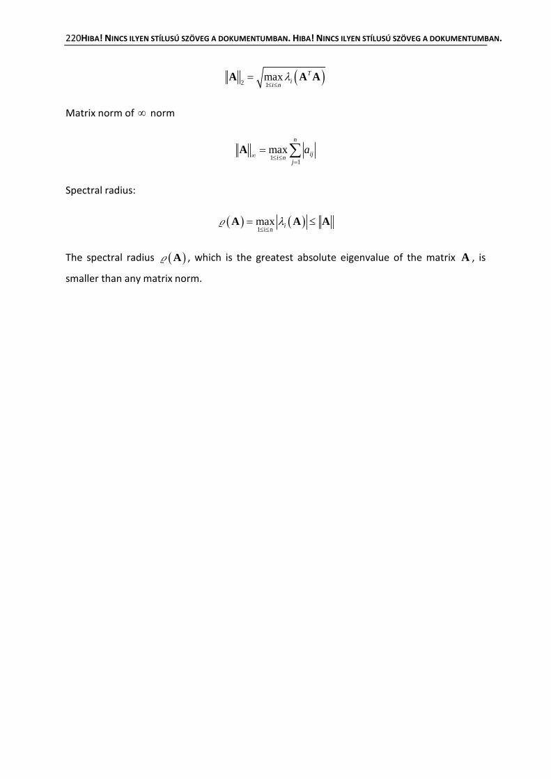
220HIBA! NINCS ILYEN STÍLUSÚ SZÖVEG A DOKUMENTUMBAN. HIBA! NINCS ILYEN STÍLUSÚ SZÖVEG A DOKUMENTUMBAN.
( )2 1max T
ii nλ
≤ ≤=A A A
Matrix norm of ∞ norm
1
1
maxn
iji nj
a∞ ≤ ≤
=
= ∑A
Spectral radius:
( ) ( )1 i nmax iλ≤ ≤
= ≤A A A
The spectral radius ( )A , which is the greatest absolute eigenvalue of the matrix A , is
smaller than any matrix norm.

221
17 Worksheets
Worksheet 1: Simple simulation model of a percussion hammer [3]
In the following a simple principle model of a percussion hammer is developed and
simulated with SIMULINK.
Fig. B.1: Percussion hammer [2]
This is a power tool designed for chiseling and breaking concrete, stone and asphalt, for
tamping, bushing and compacting in the building trade. A percussion hammer has a built-in
hammer mechanism. The striking energy is independent of operator pressure.
Electronic control allows the adjustment of the hammer force to suit the processed material
or underground [2].
Function description:
The drive piston (1) is actuated in a periodic translator motion by the crank mechanism (2).
The force transmission from the drive piston to the percussion piston (3) results from the air
cushion (4). Due to this excitation the percussion piston performs an oscillating translator
motion and axial percussions on an interposed piston, which itself impacts on the tool (In the
following the interposed piston and the tool are neglected.).

222HIBA! NINCS ILYEN STÍLUSÚ SZÖVEG A DOKUMENTUMBAN. HIBA! NINCS ILYEN STÍLUSÚ SZÖVEG A DOKUMENTUMBAN.
Analogous model:
System equations:
The rotation of the drive crank is assumed to be constant (rheonomic constraint). The
position of the drive piston is explicitly described by the length s, which is dependent on the
geometric parameters r, q as well as the angular velocity ω of the drive crank:
( ) ( )2cos 1 sinr
qs t r t q tω ω= + − .
The percussion piston can move independently in x-direction.
a) Determine the amount of degrees of freedom for this system.
b) A friction force (Coulomb’s friction) acts between the percussion piston and the wall of
the cylinder, arranged by
0 signR SF Ap xµ= − ⋅ .
A is the cross-sectional area of the cylinder, µ the dynamic friction coefficient
between piston and wall of the cylinder and p0 the ambient pressure.
c) A force acts between the drive and percussion piston due to the air cushion, which
depends on the distance sh x s− − between the piston surfaces in a nonlinear manner.
1.4
00 1l
s
lF Aph x s
= − − −
.
d) Applying the principle of linear momentum we obtain the equations of motion

HIBA! NINCS ILYEN STÍLUSÚ SZÖVEG A DOKUMENTUMBAN. HIBA! NINCS ILYEN STÍLUSÚ SZÖVEG A DOKUMENTUMBAN. 223
1.4
00 0 1S R l S
s
lmx F F Ap signx Aph x s
µ = + = − ⋅ + − − −
.
Modelling the impact process
When the percussion piston impinges on the tool respectively the header, a momentum
appears which is approximately described by a spring-damper combination with spring
constant c and damping coefficient d :
Impact S SF cx dx= − − .
However this force only acts when the percussion piston tries to penetrate into the tool
( )0sx < .
e) Consider this circumstance with an appropriate logical block in the block diagram.
Realization of the simulation
f) Develop a block diagram, which can establish a basis for the input in SIMULINK. Initially generate separate block diagrams for the motion of the drive piston, the friction force,
the air force as well as the momentum. Afterwards develop a block diagram of the
equations of motion, which imply the forces to be combined in subsystems being
dependent on ( )sx t and ( )s t .
g) Enter the block diagram in SIMULINK and perform simulations for different initial
conditions and parameters. Pore over the influence of the rotational velocity of the
crank on the function of the hammer in particular.
h) An important characteristic for the function of the hammer is the impulsion velocity of the percussion. How does the velocity change if the percussion mass is changed?
i) Determine the equivalent coefficient of restitution between percussion piston and tool
by the help of the impulsion and rebound velocity of the percussion piston.
Apply the following numerical values for the simulation:
• Percussion mass: 0.6sm kg=
• Cross-sectional area of the air cushion: 20.00151976A m=
• Air cushion height at ambient pressure: 0 0.0365l m=
• Ambient pressure: 20 100000p N m=
• Crank radius: 0.022r m=

224HIBA! NINCS ILYEN STÍLUSÚ SZÖVEG A DOKUMENTUMBAN. HIBA! NINCS ILYEN STÍLUSÚ SZÖVEG A DOKUMENTUMBAN.
• Length of con rod: 0.076q m=
• Initial position of the percussion: 0 0.0001sx m=
• Friction coefficient: 0.2µ =
• Spring constant for impact modelling: 810c N m=
• Damping coefficient for impact modelling: 7610.8d Ns m=
• Input speed: 11300 minsn −=
• Length of cylinder: 0.2h m=

HIBA! NINCS ILYEN STÍLUSÚ SZÖVEG A DOKUMENTUMBAN. HIBA! NINCS ILYEN STÍLUSÚ SZÖVEG A DOKUMENTUMBAN. 225
Wroksheet 2: Mathematical Pendulum
Mathematical pendulum
For the given mathematical pendulum (mass m , length l ) the time-dependent motion is to
be analyzed. We assume that the pendulum is pivoted in point A and can only perform a
planar motion. The acceleration of gravity acts in vertical direction. The motion of the
pendulum is influenced by a damping torque which is proportional to the respective
rotational velocity: dM dϕ= − .
Fig. B.2: Mathematical pendulum
Modelling the mathematical pendulum
a) By how many state variables can the equations of motion be definitely described? This
equals to how many degree(s) of freedom of mechanics?
b) Determine the equations of motion. Transform them to the state space.
c) Set up the system of the mathematical pendulum in a block diagram.
Solution of the state equations using MATLAB / SIMULINK:
d) Enter the plotted block diagram in SIMULINK and study the system’s behavior for the
following parameter values:
• 1m kg= ,
• 1l m= ,
• 0.1d Nms=
with the initial conditions
• 0, 2 radsϕ ϕ= = ,
• 2 , 0 rads
πϕ ϕ= = ,

226HIBA! NINCS ILYEN STÍLUSÚ SZÖVEG A DOKUMENTUMBAN. HIBA! NINCS ILYEN STÍLUSÚ SZÖVEG A DOKUMENTUMBAN.
• , 0.001 radsϕ π ϕ= = .
e) Plot the corresponding diagrams of the rotational angle and rotational velocity,
respectively versus time, as well as the phase diagrams. Experiment with different
parameters and further initial conditions.
Linearized equations of motion:
For << 1 the motion can be approximately described by linearized equations of motion.
f) Which linearization do we need to apply? Set up the linear state equations in matrix
description
g) Determine the eigenfrequency 0 and f0, respectively of the pendulum with the given
parameters from above
h) Confirm the numerical value for the eigenfrequency using MATLAB and perform a simulation of the nonlinear and linear system with suitable initial conditions. Evaluate
the error due to linearization.
Modified pendulum:
Now the pendulum is extended by a spring ( )10c N m= , see Fig. B.3.
Fig. B.3: Modified pendulum
i) Set up the nonlinear equations of motion for this system. And transform them to the
nonlinear state space.
j) What is the system’s new state of equilibrium? Determine further states of equilibrium
if they exist
k) Modify your model adequately and perform further simulations.

HIBA! NINCS ILYEN STÍLUSÚ SZÖVEG A DOKUMENTUMBAN. HIBA! NINCS ILYEN STÍLUSÚ SZÖVEG A DOKUMENTUMBAN. 227 Worksheet 3: Longitudinal oscillations of a continuous beam
The longitudinal oscillations of a continuous beam can be described by the help of the partial
differential equation
( ) ( )2
2
,u x tAu t EA
xρ
∂=
∂ .
It can be analyzed with analytical or numerical methods.
Fig. B.4: Continuous beam
By means of a steal beam ( )3 11 21 , 7850 , 2.1 10L m kg m E N mρ= = = ⋅ analyze how far
the accuracy of the eigenfrequencies, which are determined by local discretization, depends on the number of discretized elements.

228HIBA! NINCS ILYEN STÍLUSÚ SZÖVEG A DOKUMENTUMBAN. HIBA! NINCS ILYEN STÍLUSÚ SZÖVEG A DOKUMENTUMBAN.
Worksheet 4: Predator-Prey-Models
In a biotope the relationship of animals of the species B (=prey) and R (=predator) is
examined. The relationship of both species is such that R mainly feeds on B . An example
for this may be the relationship between the species fox and hare.
Which time-dependent process results for the populations of the species B and R , if the
population of B is xB(t) and the population of R is ( )Rx t ? In the following this task is solved
step-by-step.
Dynamics of a population of a species
Strictly speaking the populations of ( )Bx t and ( )Rx t can only be whole-numbered. To apply
the methods of differential calculus, we assume that ( )Bx t and ( )Rx t are differentiable
functions.
a) When can this assumption be justified?
b) Determine the current growth velocity for the population ( )x t of a breed.
c) Determine the growth rate ( )w t (differential equation!) which is defined by the
relation growth velocity
existing population.
Constant growth rate
d) Determine the simplified linear differential equation for ( )w t a≡ . What is the general
solution for this problem if ( )0 0x x= denotes the initial population?
e) Which three cases do we need to distinguish?
Due to the limits of the natural resources the exponential increase of populations is
practically not possible. For this reason a more realistic process of growth has to be
examined.
Logistic growth rate
Here we assume that the constant value of the growth rate is weakened by a component
(factor 0b > ) which is proportional to the population.
f) Set up the equation for this case (which is also known as the logistic growth rate
( )( )w t . Which population equation do we obtain now?

HIBA! NINCS ILYEN STÍLUSÚ SZÖVEG A DOKUMENTUMBAN. HIBA! NINCS ILYEN STÍLUSÚ SZÖVEG A DOKUMENTUMBAN. 229
g) Determine the general solution for this problem. Hint: Apply the method of expansion
into partial fractions. Towards which constant value does this solution converge for
t →∞ .
Dynamics of a population in a predator-prey community
Two species are considered, of which populations are denoted by the indices R (predator)
and B (prey). For the derivation of suitable growth laws the following simplified
assumptions are made:
Without predators the prey population is defined by a growth law with constant growth
rate.
The (reducing) influence of predators on the prey population is proportional to the predator
population (factor b ).
h) What is the growth rate ( )Bw t for the prey population?
Without prey the predator population would become extinct with a constant (negative)
growth rate c .
The refreshment of the growth rate of the predator population is proportional to the prey
population (factor d ).
i) What is the growth rate ( )Rw t of the predator population?
j) What system of differential equations do we obtain now? Be Bx the current
population of the prey and Rx the current population of the predator.
These equations are denoted as Volterra-Equations (according to Vito Volterra (1860-1940)).
Volterra was the one who first set up a mathematical model for the dynamics of
populations.
The Volterra-Equations cannot be solved analytically anymore. We have to resort to
numerical solution methods. Therefore MATLAB/SIMULINK is applied now.
Solution of the Volterra-Equations with MATLAB/SIMULINK
k) Set up the block diagram of the system.
l) Enter the block diagram in SIMULINK and study the system behavior for different
parameter values. Choose e.g.

230HIBA! NINCS ILYEN STÍLUSÚ SZÖVEG A DOKUMENTUMBAN. HIBA! NINCS ILYEN STÍLUSÚ SZÖVEG A DOKUMENTUMBAN.
1a b c d= = = =
2, 0.5B Rx x= = (each with thousand units)
0, 20Start Endt t= = (time units)
m) Compare with the behavior of isolated populations. The time response of predator and
prey populations is periodic for each. Determine empirically the period and show that
the predator and prey populations have the same period.
The predator-prey model with logistic growth
Here a more realistic model can also be set up, if we assume logistic growth rates:
( )B B Rw a e x b x= − − ,
( ) , , , , ,R R Bw c f x d x e f a b c d= − + + 0 .
With the base equation x wx= the logistic Volterra-System yields
2B B R R Bx ax bx x ex= − − and 2
R R B R Rx cx dx x fx= + −
Change your model accordingly and analyze the system behavior by repeating the simulation
with different sets of parameters. Particularly check, if the chronological process of the populations is still periodic.

HIBA! NINCS ILYEN STÍLUSÚ SZÖVEG A DOKUMENTUMBAN. HIBA! NINCS ILYEN STÍLUSÚ SZÖVEG A DOKUMENTUMBAN. 231 Worksheet 5: Modelling of a double pendulum with DYMOLA
Fig. B.5: a) Double pendulum b) Cut model of pendulum
Fig. B.5a shows a planar double pendulum. Each pendulum is represented by a massless link
(length l) and a point mass m at the end of the link. The modelling of this system of
pendulums has to be realized by the Multiport/Cut-Set-Method (Chapter 3 of the lecture slides). For this purpose let us analyze one pendulum which will represent the upper (1—2)
as well as the lower (2—3) part of the total system (Fig. B.5b). The following assignments are
related to Fig. B.5b.
a) Determine the geometrical constraint for the subsystem.
b) Draw the Multiport/Cut-Set-model. What are the across and through variables of the
system? c) Determine the necessary equations of motion for the pendulum.
d) Generate the Multiport/Cut-Set-model of the total system according to Fig. B.5a.
Modelling the double pendulum with DYMOLA:
e) Generate the subsystem model in the DYMOLA environment:
1. Construct the connections (Ports) for input and output signals (File/New-
/Connector). Hint: through variables are realized by the prefix flow.
2. Construct the inertial frame for the system. What are the constraints for the across variables of this inertial frame (File/New/Model).
3. Generate the subsystem of the pendulum according to the equations that you have
determined before ( )1 , 1 , g 9.81m kg l m m s= = = .
f) Test your subsystem by modelling a single pendulum and check the simulation results.

232HIBA! NINCS ILYEN STÍLUSÚ SZÖVEG A DOKUMENTUMBAN. HIBA! NINCS ILYEN STÍLUSÚ SZÖVEG A DOKUMENTUMBAN.
g) Set up the total double pendulum and compare the new results with those of subtask
2.
h) Append further pendulum elements and analyze the behavior.

HIBA! NINCS ILYEN STÍLUSÚ SZÖVEG A DOKUMENTUMBAN. HIBA! NINCS ILYEN STÍLUSÚ SZÖVEG A DOKUMENTUMBAN. 233 Worksheet 6: Oscillations of a quarter vehicle model
The equations of motion of a quarter vehicle model are
0 0 1 00
0 0 0 10
( )0A A A AS
A A A AR
A R A A AR
R R R R
c c d dx t
m m m mc
c c c d dm
m m m mu
− −= + +
− −
x x
x BA
((((((((((((
0
0 0 0
A A A A
A A A A SR
R
c c d dm m m m x
cc
− − = + −
y x
DxC
((((((((
with
01
02
3
4
A A
R R
A
R
xx xxx xxxxx
− − = =
x
a) Calculate the eigenvalues and eigenvectors with MATLAB.
b) Determine the angular eigenfrequencies of the system.
c) Determine the eigenoscillations of the system.
d) Draw the block diagram of the system.
e) Create the SIMULINK model of the system according to the block diagram.
f) The system is excited by a sinusoidal oscillation with the eigenfrequency. What
phenomenon occurs?

234HIBA! NINCS ILYEN STÍLUSÚ SZÖVEG A DOKUMENTUMBAN. HIBA! NINCS ILYEN STÍLUSÚ SZÖVEG A DOKUMENTUMBAN.
Modelling parameters
• 9.81g = gravitational acceleration 2m s
• 380Am = mass of the chassis [ ]kg
• 35Rm = mass of the wheel [ ]kg
• 325 10Ac = ⋅ spring constant of the suspension [ ]N m
• 250Ad = damping constant of the suspension [ ]Ns m
• 325 10Rc = ⋅ spring constant of the wheel [ ]N m

HIBA! NINCS ILYEN STÍLUSÚ SZÖVEG A DOKUMENTUMBAN. HIBA! NINCS ILYEN STÍLUSÚ SZÖVEG A DOKUMENTUMBAN. 235 Worksheet 7: Kinematics of a rear five-link wheel suspension
With the help of MATLAB the kinematics of the following rear five-link wheel suspension is
to be modelled (Fig. B.6).
Fig. B.6: Rear five-link wheel suspension
The vertical deflection cz of the wheel carriage is considered to be the generalized
coordinate (degree of freedom).
a) How many constraint equations are necessary to determine the position and
orientation of the wheel carriage? What are the dependent coordinates of the wheel
carriage?
Given are the position vectors to the mounting points 1 5 1 5, , , , , ,K K R R RC and RA in
respect of the vehicle reference coordinate frame FO (cp. MATLAB file ‚main.m’).
b) Determine on the basis of the given mounting points the lengths of the control arms 1l
to 5l . Set up the wheel carriage fixed vectors from RC to the points 1R to 5R in
respect of the wheel carriage reference point RC .
c) Determine the constraint equations in the form ( ) =F x 0 . Hints: Fill the constraint
equations into the prepared file ‚FiveLink.m’. The numerical solution of the constraint
equation is realized with the help of the MATLAB function ‚fsolve’. It calls ‚FiveLink.m’
and internally solves the (nonlinear) system of equation ( ) =F x 0 .
d) Draw the wheel trajectory and the deflection of the suspension depending on the
camber and toe angle.
e) Animate the wheel suspension with MATLAB.

236HIBA! NINCS ILYEN STÍLUSÚ SZÖVEG A DOKUMENTUMBAN. HIBA! NINCS ILYEN STÍLUSÚ SZÖVEG A DOKUMENTUMBAN.

237
18 Exercises
Exercise 1
Linearize the following expressions about the according working points.
a) ( )sin ϕ about 0ϕ
b) ( )cos ϕ about 0ϕ =
c) xe about 0x =
d) 21 x+ about 1 2x =
e) 2
1a x+
about 0,x a= ∈R .
Exercise 2
A cylindrical basin (cross sectional area A , water level h ) with continuous inflow iq and
outlet Aq (cross sectional area of outlet 'A ).
a) Generate the differential equations for the state variable h. b) Set up the block diagram for the system.
c) Sketch possible solutions of ( )h t for 0iq = . Which further information is necessary for
a definite solution?
Exercise 3
Transform the differential equation
2 0y y y ky+ + =
to a system of differential equations of 1. order.
Exercise 4
Linearize the system
11 1 2 2 38
2 1 2 32 2
3 2
(2 cos )( 2 )( 4) , 0
( )
x x x x xx x x a x ax a x a
= − += − + + ≠= − −

238HIBA! NINCS ILYEN STÍLUSÚ SZÖVEG A DOKUMENTUMBAN. HIBA! NINCS ILYEN STÍLUSÚ SZÖVEG A DOKUMENTUMBAN.
about its states of equilibrium.
Exercise 5
Calculate the eigenvalues and eigenvectors of the matrix
2 12 3
=
A .
Exercise 6
The following matrix is given:
2 55 3
=
A .
a) Calculate the eigenvalues , 1,2i iλ = and the eigenvectors , 1,2ix i = of the matrix.
b) Confirm by means of this example the orthogonally property of the eigenvectors:
1 2 0T =x x . How can you prove this circumstance generally for any symmetric n×n-
matrix?
c) Show that with [ ]1 2=T x x the relation
11
2
00λ
λ−
=
T AT
is valid, i. e. the similarity transformation defined by T transforms A to diagonal form.
d) Calculate by the help of subtasks a) to c) the expressions
( ) ( )sin , cos ,A A A
and confirm the relations
( ) ( )2 2sin cos+ =A A E and 2 2=A A .
e) Show that different solutions result by element-wise application of the functions sin,
cos and on the matrix A .
Exercise 7
Determine for the linear time-invariant systems

HIBA! NINCS ILYEN STÍLUSÚ SZÖVEG A DOKUMENTUMBAN. HIBA! NINCS ILYEN STÍLUSÚ SZÖVEG A DOKUMENTUMBAN. 239
1 1 1 10
2 1 2 2 20
5 , (0)2 , (0)
x x x xx x x x x= − == − − =
and 1 2 1 10
2 1 2 2 20
5 , (0)2 , (0)
x x x xx x x x x= − == − − =
a) the eigenvalues and eigenvectors,
b) the solutions for given initial conditions.
Exercise 8
The initial value problem 10 7 , (0) 10tx x e x−= − + = is given.
a) Calculate the analytical solution of the initial value problem.
b) Calculate a numerical solution in the interval [0 0.05]t< ≤ with the integration step
width 0.01h = by applying the explicit Euler method.
c) Repeat the calculation in b) for the step widths 0.001h = and 0.0001 . Compare the
error of the numerical solutions with each other and also with the analytical solutions.
Exercise 9
The differential equation 0.01 0.5 0x x x− + = with the initial conditions (0) 1x = and
(0) 0x = is given.
a) Formulate the problem as a system of equations of 1. order and calculate the
analytical solution.
b) Determine the solution of the initial value problem at the times 0.5t = and 1.0t = using the explicit Euler method. Apply the integration step width 0.5h = .
Exercise 10
The equation of motion of a spring-mass oscillator is
0mx dx cx+ + = .
Determine for the values 20.5 , 1 , 100m kg d kg s c kg s= = = and the initial values ( )0 1x =
, (0) 0x = a numerical solution in the interval [ ]0,10 with
a) the Runge-Kutta method of 2 . order,
b) the explicit Euler method.
c) Solve the subtasks a) and b) for 0d = .
Vary for the subtasks the integration step width and study the behavior of the solution.

240HIBA! NINCS ILYEN STÍLUSÚ SZÖVEG A DOKUMENTUMBAN. HIBA! NINCS ILYEN STÍLUSÚ SZÖVEG A DOKUMENTUMBAN.
Exercise 11
The initial value problem
( )2 , 0 11
xx xt
= − =+
is to be solved with the Runge-Kutta method of 4. order numerically. Find a step width h
such that the local discretization error is less than 0.00001 .
19 References
[1] C. Walteros, S. Hartmann, T. Bertram und M. Hiller, Startersimulation. Abschlussbericht, Institut für Mechatronik und Systemdynamik, Universität Duisburg-Essen, 2003.
[2] Bosch, Kraftfahrtechnisches Taschenbuch, 25. Auflage szerk., Wiesbaden: Vieweg, 2003. [3] M. Hiller, Mechanische Systeme – Eine Einführung in die analytische Mechanik und
Systemdynamik, Berlin: Springer - Hochschultexte, 1983. [4] D. Möller, Modellbildung, Simulation und Identifikation Dynamischer Systeme, Berlin: Springer-
Lehrbuch, 1992. [5] D. Ammon, Modellbildung und Systsementwicklung in der Fahrzeugdynamik, Stuttgart: Teubner
Verlag, 1997. [6] D. Schramm, M. Hiller und R. Bardini, Modellbildung und Simulation der Dynamik von
Kraftfahrzeugen, Heidelberg, New York.: Springer, Berlin, 2010. [7] H. Bossel, Systemdynamik, Braunschweig, Wiesbaden: Vieweg, 1987. [8] R. C. Rosenberg und D. C. Karnopp, Introduction to Physical System Dynamics, McGraw-Hill,
1983. [9] M. Gipser, Systemdynamik und Simulation, Stuttgart: Teubner, 1999. [10] M. Hermann, Numerik gewöhnlicher Differentialgleichungen, München: Oldenbourg, 2004. [11] H. B. Pacejka, Tyre and Vehicle Dynamics, Butterworth-Heinemann, 2002. [12] U. Ascher and L. Petzold, Computer Methods for Ordinary Differential Equations and
Differential-Algebraic Equations, Philadelphia: Siam, 1998. [13] L. F. Shampine and M. K. Gordon, Computer Solution of Ordinary Differential Equations: The
Initial value problem, San Francisco: W.H. Freeman & Co., 1975. [14] K. Popp und W. Schiehlen, Fahrzeugdynamik, Stuttgart: Teubner, 1993.

HIBA! NINCS ILYEN STÍLUSÚ SZÖVEG A DOKUMENTUMBAN. HIBA! NINCS ILYEN STÍLUSÚ SZÖVEG A DOKUMENTUMBAN. 241 [15] P. C. Müller and W. O. Schiehlen, Lineare Schwingungen, Wiesbaden: Aka¬de¬mi¬sche
Verlagsanstalt, 1976. [16] J. Stoer und R. Bulirsch, Numerische Mathematik 2, Berlin, Heidelberg, New York: Springer,
2005. [17] H. Bossel, Modellbildung und Simulation, Braunschweig: Vieweg, 1992. [18] DIN, 1226 Regelungstechnische Systeme. [19] E. Freund, Regelungssysteme im Zustandsraum I, München: Oldenbourg, 1987. [20] J. D. Lambert, Computational Methods in Ordinary Differential Equations, Chichester: Wiley,
1979. [21] F. Pfeiffer, Einführung in die Dynamik, Stuttgart: Teubner, 1989. [22] H. Schlitt, Regelungstechnik, Würzburg: Vogel-Fachbuch, 1988. [23] J. Stoer, Numerische Mathematik 1, Berlin, Heidelberg, New York: Springer, 2004.