Reduction of Compound Lotteries with

Objective Probabilities: Theory and Evidence

by

Glenn W. Harrison, Jimmy Martínez-Correa and J. Todd Swarthout †

March 2012

ABSTRACT.

The reduction of compound lotteries (ROCL) has assumed a central role in the evaluation ofbehavior towards risk and uncertainty. We present experimental evidence on its validity in thedomain of objective probabilities. Our experiment explicitly recognizes the impact that the randomlottery incentive mechanism payment procedure may have on preferences, and so we collect datausing both “1-in-1” and “1-in-K” payment procedures, where K>1. We do not find violations ofROCL when subjects are presented with only one choice that is played for money. However, whenindividuals are presented with many choices and random lottery incentive mechanism is used toselect one choice for payoff, we do find violations of ROCL. These results are supported by bothnon-parametric analysis of choice patterns, as well as structural estimation of latent preferences. Wefind evidence that the model that best describes behavior when subjects make only one choice is theRank-Dependent Utility model. When subjects face many choices, their behavior is bettercharacterized by our source-dependent version of the Rank-Dependent Utility model which canaccount for violations of ROCL. We conclude that payment protocols can create distortions inexperimental tests of basic axioms of decision theory.

† Department of Risk Management & Insurance and Center for the Economic Analysis of Risk,Robinson College of Business, Georgia State University, USA (Harrison); Department of RiskManagement & Insurance, Robinson College of Business, Georgia State University, USA (Martínez-Correa); and Department of Economics, Andrew Young School of Policy Studies, Georgia StateUniversity, USA (Swarthout). E-mail contacts: gharrison@gsu.edu, jimmigan@gmail.com andswarthout@gsu.edu.

Table of Contents

1. Theory . . . . . . . . . . . . . . . . . . . . . . . . . . . . . . . . . . . . . . . . . . . . . . . . . . . . . . . . . . . . . . . . . . . . . . . -3-A. Basic Axioms . . . . . . . . . . . . . . . . . . . . . . . . . . . . . . . . . . . . . . . . . . . . . . . . . . . . . . . . . . . -3-B. Experimental Payment Protocols . . . . . . . . . . . . . . . . . . . . . . . . . . . . . . . . . . . . . . . . . . . -5-

2. Experiment . . . . . . . . . . . . . . . . . . . . . . . . . . . . . . . . . . . . . . . . . . . . . . . . . . . . . . . . . . . . . . . . . . . -7-A. Lottery Parameters . . . . . . . . . . . . . . . . . . . . . . . . . . . . . . . . . . . . . . . . . . . . . . . . . . . . . . -7-B. Experimental Procedures . . . . . . . . . . . . . . . . . . . . . . . . . . . . . . . . . . . . . . . . . . . . . . . . . -8-C. Evaluation of Hypotheses . . . . . . . . . . . . . . . . . . . . . . . . . . . . . . . . . . . . . . . . . . . . . . . . -10-

3. Non-Parametric Analysis of Choice Patterns . . . . . . . . . . . . . . . . . . . . . . . . . . . . . . . . . . . . . . . -11-A. Choice Patterns Where ROCL Predicts Indifference . . . . . . . . . . . . . . . . . . . . . . . . . . -11-B. Choice Patterns Where ROCL Predicts Consistent Choices . . . . . . . . . . . . . . . . . . . . . -14-

4. Estimated Preferences from Observed Choices . . . . . . . . . . . . . . . . . . . . . . . . . . . . . . . . . . . . . -17-A. Econometric Specification . . . . . . . . . . . . . . . . . . . . . . . . . . . . . . . . . . . . . . . . . . . . . . . -17-B. Estimates . . . . . . . . . . . . . . . . . . . . . . . . . . . . . . . . . . . . . . . . . . . . . . . . . . . . . . . . . . . . . -23-

5. Conclusions . . . . . . . . . . . . . . . . . . . . . . . . . . . . . . . . . . . . . . . . . . . . . . . . . . . . . . . . . . . . . . . . . . -26-

References . . . . . . . . . . . . . . . . . . . . . . . . . . . . . . . . . . . . . . . . . . . . . . . . . . . . . . . . . . . . . . . . . . . . . -40-

Appendix A: Instructions (NOT FOR PUBLICATION) . . . . . . . . . . . . . . . . . . . . . . . . . . . . . . . -44-

Appendix B: Parameters . . . . . . . . . . . . . . . . . . . . . . . . . . . . . . . . . . . . . . . . . . . . . . . . . . . . . . . . . . -52-

Appendix C: Related Literature (NOT FOR PUBLICATION) . . . . . . . . . . . . . . . . . . . . . . . . . . -62-

Appendix D: Nonparametric Tests (NOT FOR PUBLICATION) . . . . . . . . . . . . . . . . . . . . . . . -65-

Appendix E: Additional Econometric Analysis (NOT FOR PUBLICATION) . . . . . . . . . . . . . . -74-

Appendix F: Detailed Binomial Test Results (NOT FOR PUBLICATION) . . . . . . . . . . . . . . . -80-

Appendix G: Detailed Fisher Exact Test Results (NOT FOR PUBLICATION) . . . . . . . . . . . . -82-

Appendix H: Detailed McNemar Test Results (NOT FOR PUBLICATION) . . . . . . . . . . . . . . . -85-

Appendix I: Detailed Wald Test Results for Predictions (NOT FOR PUBLICATION) . . . . . . . -93-

The reduction of compound lotteries has assumed a central role in the evaluation of behavior

towards risk, uncertainty and ambiguity. We present experimental evidence on its validity in domains

defined over objective probabilities, as a prelude to evaluating it over subjective probabilities.

Because of the attention paid to violations of the Independence Axiom, it is noteworthy that

early formal concerns with the possibility of a “utility or disutility for gambling” centered around the

Reduction of Compound Lotteries (ROCL) axiom.1 Von Neumann and Morgenstern [1953, p. 28]

commented on the possibility of allowing for a (dis)utility of gambling component in their preference

representation:

Do not our postulates introduce, in some oblique way, the hypotheses which bring in themathematical expectation [of utility]? More specifically: May there not exist in anindividual a (positive or negative) utility of the mere act of ‘taking a chance,’ of gambling,which the use of the mathematical expectation obliterates? How did our axioms (3:A)-(3:C) get around this possibility? As far as we can see, our postulates (3:A)-(3:C) do notattempt to avoid it. Even the one that gets closest to excluding the ‘utility of gambling’ -(3:C:b)- seems to be plausible and legitimate - unless a much more refined system ofpsychology is used than the one now available for the purposes of economics [...] Since(3:A)-(3:C) secure that the necessary construction [of utility] can be carried out, conceptslike a ‘specific utility of gambling’ cannot be formulated free of contradiction on thislevel.

On the very last page of their magnus opus, von Neumann and Morgenstern [1953; p. 632] propose that if

their postulate (3:C:b), which is the ROCL, is relaxed, one could indeed allow for a specific utility for the

act of gambling:

It seems probable, that the really critical group of axioms is (3:C) - or, more specifically,the axiom (3:C:b). This axiom expresses the combination rule for multiple chancealternatives, and it is plausible, that a specific utility or disutility of gambling can onlyexist if this simple combination rule is abandoned. Some change of the system [of

1 The issue of the (dis)utility of gambling goes back at least as far as Pascal, who argued in his Penséesthat “people distinguish between the pleasure or displeasure of chance (uncertainty) and the objectiveevaluation of the worth of the gamble from the perspective of its consequences” (see Luce and Marley [2000;p. 102]). Referring to the ability of bets to elicit beliefs, Ramsey [1926] claims that “[t]his method I regard asfundamentally sound; but it suffers from being insufficiently general, and from being necessarily inexact. It isinexact partly [...] because the person may have a special eagerness or reluctance to bet, because he eitherenjoys or dislikes excitement or for any other reason, e.g. to make a book. The difficulty is like that ofseparating two different cooperating forces” (from the reprint in Kyburg and Smokler [1964; p. 73]).

-1-

axioms] (3:A)-(3:B), at any rate involving the abandonment or at least a radicalmodification of (3:C:b), may perhaps lead to a mathematically complete and satisfactorycalculus of utilities which allows for the possibility of a specific utility or disutility ofgambling. It is hoped that a way will be found to achieve this, but the mathematicaldifficulties seem to be considerable.

Thus, the relaxation of the ROCL axiom opens the door to the possibility of having a distinct

(dis)utility for the act of gambling with objective probabilities.2 Fellner [1961][1963] and Smith [1969]

used similar reasoning to offer an explanation for several of the Ellsberg [1961] paradoxes.

This argument rests on the hypothesis that subjects potentially view simple and compound

random processes differently. If this hypothesis is true, it could explain why people prefer risky over

ambiguous gambles in the thought experiments of Ellsberg [1961]. Fellner [1961][1963] and Smith

[1969] believed that if a subject could exhibit utility or disutility of gambling she may also use different

utility functions to make decisions under different processes. Smith [1969] went further and explicitly

conjectured that a compound lottery defined over objective probabilities, and its actuarially-equivalent

lottery over objective probabilities, might be viewed by decision makers as two different random

processes. In fact, he proposed a preference representation that allowed people to have different utility

functions for different random processes. We use this conjectured preference representation to test for

violations of ROCL.

One fundamental methodological problem with tests of the ROCL assumption, whether or not

the context is objective or subjective probabilities, is that one cannot use incentives for decision makers

that rely on the validity of ROCL. This means, in effect, that experiments must be conducted in which a

subject has one, and only one, choice.3 Apart from the expense and time of collecting data at such a

2 Of course, it is of some comfort to the egos of modern theorists that no less than von Neumannand Morganstern at least viewed it as a serious mathematical challenge.

3 One alternative is to present the decision maker with several tasks at once and evaluate the portfoliochosen, or to present the decision maker with several tasks in sequence and account for wealth effects.Neither is attractive, since they each raise a number of (fascinating) theoretical confounds to the interpretationof observed behavior. One uninteresting alternative is not to pay the decision maker for the outcomes of thetask.

-2-

pace, this also means that all evaluations have to be on a between-subjects basis, implying the necessity

of modeling assumptions about heterogeneity in behavior.

In sections 1 and 2 we define the theory and experimental tasks used to examine ROCL in the

context of objective probabilities. In section 3 and 4 we present evidence from our experiment. We find

no violations of ROCL when subjects are presented with one and only one choice, and that their behavior

is better characterized by the Rank-Dependent Utility model (RDU) rather than Expected Utility Theory

(EUT). However, we do find violations of ROCL when many choices are given to each subject and the

random lottery incentive mechanism (RLIM) is used as the payment protocol. Under RLIM, behavior is

better characterized by our source-dependent version of RDU that can account for violations of ROCL.

Section 5 draws conclusions for modeling, experimental design, and inference about decision making.

1. Theory

A. Basic Axioms

Following Segal [1988][1990][1992], we distinguish between three axioms. In words, the

Reduction of Compound Lotteries axiom states that a decision-maker is indifferent between a

compound lottery and the actuarially-equivalent simple lottery in which the probabilities of the two

stages of the compound lottery have been multiplied out. To use the language of Samuelson [1952;

p.671], the former generates a compound income-probability-situation, and the latter defines an associated income-

probability-situation, and that “...only algebra, not human behavior, is involved in this definition.”

To state this more explicitly, with notation to be used to state all axioms, let X, Y and Z denote

simple lotteries, A and B denote compound lotteries, ™ express strict preference, and - express

indifference. Then the ROCL axiom says that A - X if the probabilities and prizes in X are the

actuarially-equivalent probabilities and prizes from A. Thus if A is the compound lottery that pays

“double or nothing” from the outcome of the lottery that pays $10 if a coin flip is a head and $2 if the

-3-

coin flip is a tail, then X would be the lottery that pays $20 with probability ½×½ = ¼, $4 with

probability ½×½ = ¼, and nothing with probability ½. From an observational perspective, one must

see choices between compound lotteries and actuarially-equivalent simple lotteries to test ROCL.

The Compound Independence Axiom (CIA) states that two compound lotteries, each formed

from a simple lottery by adding a positive common lottery with the same probability, will exhibit the

same preference ordering as the simple lotteries. This is a statement that the ordering of the two

constructed compound lotteries will be the same as the ordering of the different simple lotteries that

distinguish the compound lotteries, provided that the common prize in the compound lotteries is the

same and has the same (compound lottery) probability. It says nothing about how the compound

lotteries are to be evaluated, and in particular it does not assume ROCL. It only restricts the preference

ordering of the two constructed compound lotteries to match the preference ordering of the original simple

lotteries.

The CIA says that if A is the compound lottery giving the simple lottery X with probability α

and the simple lottery Z with probability (1-α), and B is the compound lottery giving the simple lottery Y

with probability α and the simple lottery Z with probability (1-α), then A ™ B iff X ™ Y œ α 0 (0,1). The

construction of the two compound lotteries A and B has the “independence axiom” cadence of the

common prize Z with a common probability (1-α), but the implication is only that the ordering of the

compound and constituent simple lotteries are the same.4

Finally, the Mixture Independence Axiom (MIA) says that the preference ordering of two

simple lotteries must be the same as the actuarially-equivalent simple lottery formed by adding a

4 For example, Segal [1992; p.170] defines the CIA by assuming that the second-stage lotteries arereplaced by their certainty-equivalent, “throwing away” information about the second-stage probabilitiesbefore one examines the first-stage probabilities at all. Hence one cannot then define the actuarially-equivalentsimple lottery, by construction, since the informational bridge to that calculation has been burnt. Thecertainty-equivalent could have been generated by any model of decision making under risk, such as RDU orProspect Theory.

-4-

common outcome in a compound lottery of each of the simple lotteries, where the common outcome

has the same value and the same (compound lottery) probability. So stated, it is clear that the MIA

strengthens the CIA by making a definite statement that the constructed compound lotteries are to be

evaluated in a way that is ROCL-consistent. Construction of the compound lottery in the MIA is

actually implicit: the axiom only makes observable statements about two pairs of simple lotteries. To

restate Samuelson’s point about the definition of ROCL, the experimenter testing the MIA could have

constructed the associated income-probability-situation without knowing the risk preferences of the

individual (although the experimenter would need to know how to multiply).

The MIA says that X ™ Y iff the actuarially-equivalent simple lottery of αX + (1-α)Z is strictly

preferred to the actuarially-equivalent simple lottery of αY + (1-α)Z, œ α 0 (0,1). The verbose language

used to state the axiom makes it clear that MIA embeds ROCL into the usual independence axiom

construction with a common prize Z and a common probability (1-α) for that prize.

The reason these three axioms are important is that the failure of MIA does not imply the failure

of CIA and ROCL. It does imply the failure of one or the other, but it is far from obvious which one.

Indeed, one could imagine some individuals or task domains where only CIA might fail, only ROCL

might fail, or both might fail. Because specific types of failures of ROCL lie at the heart of many

important models of decision-making under uncertainty and ambiguity, it is critical to keep the axioms

distinct as a theoretical and experimental matter.

B. Experimental Payment Protocols

Turning now to experimental procedures, as a matter of theory the most popular payment

protocol assumes the validity of MIA. This payment protocol is called the Random Lottery Incentive

Mechanism (RLIM). It entails the subject undertaking K>1 tasks and then one of the K choices being

selected at random to be played out. Typically, and without loss of generality, assume that the selection

-5-

of the kth task to be played out uses a uniform distribution over the K tasks. Since the other K-1 tasks

will generate a payoff of zero, the payment protocol can be seen as a compound lottery that assigns

probability α = 1/K to the selected task and (1-α) = (1-(1/K)) to the other K-1 tasks as a whole. If the

task consists of binary choices between simple lotteries X and Y, then the RLIM can be immediately

seen to entail an application of MIA, where Z = U($0) and (1-α) = (1-(1/K)), for the utility function

U(@). Hence, under MIA, the preference ordering of X and Y is independent of all of the choices in the

other tasks (Holt [1986]).

The need to assume the MIA can be avoided by setting K=1, and asking each subject to answer

one binary choice task for payment. Unfortunately, this comes at the cost of another assumption if one

wants to compare choice patterns over two simple lottery pairs, as in most of the popular tests of EUT

such as the Allais Paradox and Common Ratio test: the assumption that risk preferences across subjects

are the same. This is a strong assumption, obviously, and one that leads to inferential tradeoffs in terms

of the “power” of tests of EUT relying on randomization that will vary with sample size. Sadly, plausible

estimates of the degree of heterogeneity in the typical population imply massive sample sizes for

reasonable power, well beyond those of most experiments.

The assumption of homogeneous preferences can be diluted, however, by changing it to a

conditional form: that risk preferences are homogeneous conditional on a finite set of observable

characteristics.5 Although this sounds like an econometric assumption, and it certainly has statistical

implications, it is as much a matter of (operationally meaningful) theory as formal statements of the

CIA, ROCL and MIA.

5 Another way of diluting the assumption is to posit some (flexible) parametric form for thedistribution of risk attitudes in the population, and use econometric methods that allow one to estimate theextent of that unobserved heterogeneity across individuals. Tools for this “random coefficients” approach toestimating non-linear preference functionals are developed in Andersen, Harrison, Hole, Lau and Rutström[2010].

-6-

2. Experiment

A. Lottery Parameters

We designed our battery of lotteries to allow for specific types of comparisons needed for testing

ROCL. Beginning with a given simple (S) lottery and compound (C) lottery, we next create an actuarially-

equivalent (AE) lottery from the C lottery, and then we construct three pairs of lotteries: a S-C pair, a S-

AE pair, and an AE-C pair. By repeating this process 15 times, we create a battery of lotteries consisting

of 15 S-C pairs shown in Table B2, 15 S-AE pairs shown in Table B3, and 10 AE-C pairs6 shown in

Table B4. See Appendix B for additional information regarding the creation of these lotteries.

Figure 1 displays the coverage of lotteries in the Marschak-Machina triangle, covering all of the

contexts used.7 Probabilities were drawn from 0, ¼, ½, ¾ and 1, and the final prizes from $0, $10, $20,

$35 and $70. We use the familiar “Double or Nothing” (DON) procedure for creating compound

lotteries. So, the first-stage prizes displayed in a compound lottery were drawn from $5, $10, $17.50 and

$35, and then the second-stage DON procedure yields the set of final prizes given above.

The majority of our compound lotteries use a conditional version of DON in the sense that the

initial lottery will trigger the double or nothing option that the subject will face only if a particular

outcome is realized in the initial lottery. For example, consider the compound lottery formed by an

initial lottery that pays $10 and $20 with equal probability and the option of playing DON if the

outcome of the initial lottery is $10, implying a payoff of $20 or $0 with equal chance if the DON stage is

reached. If the initial outcome is $20, there is no DON option beyond that. The right panel of Figure 2

shows a tree representation of the latter compound lottery where the initial lottery is depicted in the first

stage and the DON lottery is depicted in the second stage of the compound lottery if reached. The left

6 The lottery battery contains only 10 AE-C lottery pairs because some of the 15 S-C lottery pairsshared the same compound lottery.

7 Decision screens were presented to subjects in color. Black borders were added to each pie slice inFigures 1, 2 and 3 to facilitate black-and-white viewing.

-7-

panel of Figure 2 shows the corresponding actuarially-equivalent simple lottery which offers $20 with

probability ¾ and $0 with probability ¼.

The conditional DON lottery allows us to obtain good coverage in terms of prizes and

probabilities and to maintain a simple random processes for the initial lottery and the DON option. One

can construct a myriad of compound lotteries with only two components: (1) initial lotteries that pay

two outcomes with 50:50 odds or pay a given stake with certainty; and (2) a conditional DON which

pays double a predetermined amount with 50% probability or nothing with equal chance. Using only the

unconditional DON option would impose an a priori restriction on the coverage within the Marschak-

Machina triangle.

B. Experimental Procedures

We implement two between-subjects treatments. We call one treatment “Pay 1-in-1” (1-in-1)

and the other “Pay 1-in-40” (1-in-40). Table 1 summarizes our experimental design and the sample size

of subjects and choices in each treatment.

In the 1-in-1 treatment, each subject faces a single choice over two lotteries. The lottery pair presented

to each subject is randomly selected from the battery of 40 lottery pairs. The lottery chosen by the

subject is then played out and the subject receives the realized monetary outcome. There are no other

salient tasks, before or after a subject’s binary choice, that affect the outcome. Further, there is no other

activity that may contribute to learning about decision making in this context.

In the 1-in-40 treatment, each subject faces choices over all 40 lottery pairs, with the order of the

pairs randomly shuffled for each subject. After all choices have been made, one choice is randomly

selected for payment using the RLIM, with each choice having a 1-in-40 chance of being selected. The

selected choice is then played out and the subject receives the realized monetary outcome, again with no

other salient tasks. This treatment is potentially different from the 1-in-1 treatment in the absence of

-8-

ROCL, since the RLIM induces a compound lottery consisting of a 1-in-40 chance for each of the 40

chosen lotteries to be selected for payment.

The general procedures during an experiment session were as follows. Upon arrival at the

laboratory, each subject drew a number from a box which determined random seating position within

the laboratory. After being seated and signing the informed consent document, subjects were given

printed instructions and allowed sufficient time to read these instructions8. Once subjects had finished

reading the instructions, an experimenter at the front of the room read aloud the instructions, word for

word. Then the randomizing devices9 were explained and projected onto the front screen and three large

flat-screen monitors spread throughout the laboratory. The subjects were then presented with lottery

choices, followed by a non-salient demographic questionnaire that did not affect final payoffs. Next,

each subject was approached by an experimenter who would provide dice so for the subject to roll and

determine her own payoff. If a DON stage was reached, a subject would flip a U.S. quarter dollar coin

to determine the final outcome of the lottery. Finally, subjects then left the laboratory and were privately

paid their earnings: a $7.50 participation payment in addition to the monetary outcome of the realized

lottery.

We used software created in Visual Basic .NET to present lotteries to subjects and record their

choices. Figure 3 shows an example of the subject display of an AE-C lottery pair. The first and second

stages of the compound lottery, like the one depicted in Figure 2, are presented as an initial lottery,

represented by the pie on the right of Figure 3, that has a DON option identified by text. The pie chart

on the left of Figure 3 shows the AE lottery of the paired C lottery on the right. Figure 4 shows an

example of the subject display of a S-C lottery pair, and Figure 5 shows an example of the subject

8 Appendix A provides complete subject instructions.9 Only physical randomizing devices were used, and these devices were demonstrated prior to any

decisions. In the 1-in-40 treatment, two 10-sided dice were rolled by each subject until a number between 1and 40 came up to select the relevant choice for payment. Subjects in both treatments would roll the two 10-sided dice (a second roll in the case of the 1-in-40 treatment) to determine the outcome of the chosen lottery.

-9-

display of a S-AE lottery pair.

C. Evaluation of Hypotheses

If the subjects in both treatments have the same risk preferences and behavior is consistent with

ROCL, we should see the same pattern of decisions for comparable lottery pairs across the two

treatments. The same pattern should also be observed as one characterizes heterogeneity of individual

preferences towards risk, although these inferences depend on the validity of the manner in which

heterogeneity is modeled.

Nothing here assumes that behavior is characterized by EUT. The validity of EUT requires both

ROCL and CIA, and the validity of ROCL does not imply the validity of CIA. So when we say that risk

preferences should be the same in the two treatments under ROCL, these are simply statements about

the Arrow-Pratt risk premium, and not about how that is decomposed into explanations that rely on

diminishing marginal utility or probability weighting. We later analyze the decomposition of the risk

premium as well as the nature of any violation of ROCL.

Our method of evaluation is twofold. First, we use non-parametric tests to evaluate the choice

patterns of subjects. Our experimental design allows us to evaluate ROCL using choice patterns in two

ways: (1) directly examine choice patterns in AE-C lottery pairs where ROCL predicts indifference; and

(2) examine the choice patterns across the linked S-C and S-AE lottery pairs. We have 15 tests, one for

each linked pair of lottery pairs, as well as a pooled test over all 15 pairs of pairs. We are agnostic as to

the choice pattern itself: if subjects have a clear preference for S over C in a given lottery pair, then

under ROCL we should see the same preference for the identical S over the AE in the linked lottery

pair.

For our second method of evaluation of ROCL, we estimate structural models of risk

preferences and test if the risk preference parameters depend on whether a C or an AE lottery is being

-10-

evaluated. This method does not assume EUT, and indeed we allow non-EUT specifications. We

specify a source-dependent form of utility and probability weighting function and test for violations of

ROCL by determining if the subjects evaluate simple and compound lotteries differently.

In both of our methods of evaluation of ROCL, we use data from the 1-in-1 treatment and the

1-in-40 treatment which uses RLIM as the payment protocol. Of course, analysis of the data from the 1-

in-40 treatment requires us to assume incentive compatibility with respect to the experiment payment

protocol. However, by also analyzing choices from the 1-in-1 treatment we can test if the RLIM itself

creates distortions that could be confounded with violations of ROCL. We conclude with discussion of

the relative advantages and disadvantages of the econometric tests and the choice pattern tests.

3. Non-Parametric Analysis of Choice Patterns

A. Choice Patterns Where ROCL Predicts Indifference

The basic prediction of ROCL is that subjects who satisfy the axiom are indifferent between a

compound lottery and its actuarially-equivalent lottery. We analyze the observed responses from subjects

who were presented with any of the 10 pairs that contained both a C lottery and its AE lottery.10 First,

we study the responses from the 32 subjects who were presented with an AE-C pair in 1-in-1 treatment.

Then, we study the 620 responses from the 62 subjects who each were presented with all of the 10 AE-

C pairs in the 1-in-40 treatment.

We analyze the data separately because, in contrast to the 1-in-40 treatment, any conclusion

drawn from the 1-in-1 treatment do not depend on the incentive compatibility of the RLIM. We want to

control for the possibility that the observed choice patterns in the 1-in-40 treatment are affected by this

payment protocol.11 By analyzing data from the 1-in-1 treatment only, we avoid any possible confounds

10 These are pairs 31 through 40 of Table B4.11 An additional consideration is that our interface did not allow expression of indifference, so we test

for equal proportions of expressions of strict preference. Even if we had allowed direct expression of

-11-

created by the RLIM.

Our null hypothesis is that subjects behave according to ROCL. ROCL predicts that a subject is

indifferent between a C lottery and its paired AE lottery, and therefore we should observe equiprobable

response proportions between C and AE lotteries in our 10 AE-C pairs. ROCL is violated if, for a given

AE-C lottery pair, we observe that the proportion C lottery choices is significantly different from the

proportion of AE lottery choices.

We do not find statistical evidence to reject the basic ROCL prediction of indifference in the 1-

in-1 treatment, although we do find statistical evidence to support violations of ROCL in the 1-in-40

treatment. Thus, giving many lottery pairs to individuals and using the RLIM to select one choice at

random for payoff create distortions in the individual decision-making process that can be confounded

with violations of ROCL.

Analysis of Data from the 1-in-1 Treatment. We use a generalized version of the Fisher Exact

test to jointly test the null hypothesis that the proportion of subjects who chose the C lottery over the

AE lottery in each of the AE-C lottery pairs are the same, as well as the Binomial Probability test to

evaluate our null hypothesis of equiprobable choice in each of the AE-C lottery pairs.

We do not observe statistically significant violations of the ROCL indifference prediction in the

1-in-1 treatment. Table 2 presents the generalized Fisher Exact test for all AE-C lottery pair choices, and

the test’s p-value of 0.342 provides support for the null hypothesis. We see from this test that the

proportions are the same across pairs. We now use a series of Binomial Probability tests to see if the

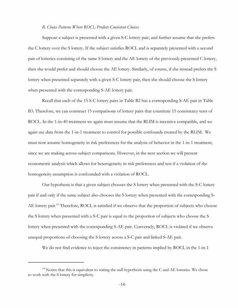
proportions are different from 50%. Table 3 shows the Binomial Probability test applied individually to

each of the AE-C lottery pairs for which we have observations. We see no evidence to reject the null

indifference, we have no way of knowing if subjects were in fact indifferent but preferred to use their ownrandomizing device (in their heads). The same issue confronts tests of mixed strategies in strategic games.

-12-

hypothesis that subjects chose the C and the AE lotteries in equal proportions, as all p-values are

insignificant at any reasonable level of confidence. The results of both of these tests suggest that ROCL

is satisfied in the 1-in-1 treatment.

Analysis of Data from the 1-in-40 Treatment The strategy to test the ROCL prediction of

indifference in this treatment is different from the one used in the 1-in-1 treatment, given the repeated

measures we have for each subject in the 1-in-40 treatment. We now use the Cochran Q test to evaluate

whether the proportion of subjects who choose the C lottery is the same in each of the 10 AE-C lottery

pairs.12 A significant difference of proportions identified by this test is sufficient to reject the null

prediction of indifference.13 Of course, an insignificant difference of proportions would require us to

additionally verify that the common proportion across pairs the pairs is indeed 50% before we fail to

reject the null hypothesis of indifference.

We observe an overall violation of the ROCL indifference prediction in the 1-in-40 treatment.

Table 4 reports the results of the Cochran Q test, as well as summary statistics of the information used

to conduct the test. The Cochran Q test yields a p-value of less than 0.0001, which strongly suggests

rejection of the null hypothesis of equiprobable proportions. We conclude, for at least for one of the

AE-C lottery pairs, that the proportion of subjects who chose the C lottery is not equal to 50%. This

result is a violation of ROCL and we cannot claim that subjects satisfy ROCL and choose at random in

all of the 10 AE-C lottery pairs in the 1-in-40 treatment.

12 The Binomial Probability test is inappropriate in this setting, as it assumes independentobservations. Obviously, observations are not independent when each subject makes 40 choices in thistreatment.

13 For example, suppose there were only 2 AE-C lottery pairs. If the Cochran Q test finds asignificant difference, we conclude that the proportion of subjects choosing the C lottery is not the same inthe two lottery pairs. Therefore, even if the proportion for one of the pairs was truly equal to 50%, the testresult would imply that the other proportion is not statistically equal to 50%, and thus indifference fails.

-13-

B. Choice Patterns Where ROCL Predicts Consistent Choices

Suppose a subject is presented with a given S-C lottery pair, and further assume that she prefers

the C lottery over the S lottery. If the subject satisfies ROCL and is separately presented with a second

pair of lotteries consisting of the same S lottery and the AE lottery of the previously-presented C lottery,

then she would prefer and should choose the AE lottery. Similarly, of course, if she instead prefers the S

lottery when presented separately with a given S-C lottery pair, then she should choose the S lottery

when presented with the corresponding S-AE lottery pair.

Recall that each of the 15 S-C lottery pairs in Table B2 has a corresponding S-AE pair in Table

B3. Therefore, we can construct 15 comparisons of lottery pairs that constitute 15 consistency tests of

ROCL. In the 1-in-40 treatment we again must assume that the RLIM is incentive compatible, and we

again use data from the 1-in-1 treatment to control for possible confounds created by the RLIM. We

must now assume homogeneity in risk preferences for the analysis of behavior in the 1-in-1 treatment,

since we are making across-subject comparisons. However, in the next section we will present

econometric analysis which allows for heterogeneity in risk preferences and test if a violation of the

homogeneity assumption is confounded with a violation of ROCL.

Our hypothesis is that a given subject chooses the S lottery when presented with the S-C lottery

pair if and only if the same subject also chooses the S lottery when presented with the corresponding S-

AE lottery pair.14 Therefore, ROCL is satisfied if we observe that the proportion of subjects who choose

the S lottery when presented with a S-C pair is equal to the proportion of subjects who choose the S

lottery when presented with the corresponding S-AE pair. Conversely, ROCL is violated if we observe

unequal proportions of choosing the S lottery across a S-C pair and linked S-AE pair.

We do not find evidence to reject the consistency in patterns implied by ROCL in the 1-in-1

14 Notice that this is equivalent to stating the null hypothesis using the C and AE lotteries. We choseto work with the S lottery for simplicity.

-14-

treatment, while we do find evidence of violations of ROCL in the 1-in-40 treatment. As in the case of

the ROCL indifference prediction, we conclude that giving many lottery pairs to individuals and using

the RLIM to select one choice at random for payoff create distortions in the individual choice making

process that can be confounded with violations of ROCL.

Analysis of Data from the 1-in-1 Treatment We use the Cochran-Mantel-Haenszel (CMH) test

to test the joint hypothesis that in all of the 15 paired comparisons, subjects choose in the same

proportion the S lottery when presented with the S-C lottery pair and its linked S-AE lottery pair.15 If

the CMH test rejects the null hypothesis, then we interpret this as evidence of overall ROCL-

inconsistent observed behavior. We also use the Fisher Exact test to evaluate individually the

consistency predicted by ROCL in each of the 15 linked comparisons of S-C pairs and S-AE pairs for

which we have enough data to conduct the test.

We do not reject the ROCL consistency prediction. The CMH test does not reject the joint null

hypothesis that the proportion of subjects chose the S lottery when they were presented with any given

S-C pair is equal to the proportion of subjects that chose the S lottery when they were presented with

the corresponding S-AE pair. The χ2-statistic for the CMH test with the continuity correction16 is equal

to 2.393 with a corresponding p-value of 0.122. Similarly, the Fisher Exact tests presented in Table 5

show only in one comparison the p-value is less than 0.05. These results suggest that the ROCL

consistency prediction holds in the 1-in-1 treatment. However, as we

mentioned previously, this conclusion relies on the assumption of homogeneity in preferences.

15 The proportion of subjects who choose the S lottery when presented with a S-C pair, or its pairedS-AE lottery pair, has to be equal within each paired comparison, but can differ across comparisons. Moreformally, the CMH test evaluates the null hypothesis that the odds ratio of each of the 15 contingency tablesconstructed from the 15 paired comparisons are jointly equal to 1.

16 We follow Li, Simon and Gart [1979] and use the continuity correction to avoid possiblemisleading conclusions from the test in small samples.

-15-

Analysis of Data from the 1-in-40 Treatment We use the Cochran Q test coupled with the

Bonferroni-Dunn (B-D) correction procedure17 to test the hypothesis that subjects choose the S lottery

in the same proportion when presented with linked S-C and S-AE lottery pairs. The B-D procedure

takes into account repeated comparisons and allows us to maintain a familywise error rate across the 15

paired comparisons of S-C and S-AE lottery pairs.

We find evidence to reject the ROCL consistency prediction. Table 6 shows the results of the B-

D method18 for each of the 15 paired comparisons. Table 6 provides evidence that with a 5% familywise

error rate, subjects choose the S lottery in different proportions across linked S-C lottery pairs and S-AE

lottery pairs in two comparisons: Pair 1 vs. Pair 16 and Pair 3 vs. Pair 18. This implies that the ROCL

prediction of consistency is rejected in 2 of our 15 consistency comparisons.

We are also interested in studying the patterns of violations of ROCL. A pattern inconsistent

with ROCL would be subjects choosing the S lottery when presented with a given S-C lottery pair, but

switching to prefer the AE lottery when presented with the matched S-AE pair. We construct 2 × 2

contingency tables that show the number of subjects in any given matched pair who exhibit each of the

four possible choice patterns: (i) always choosing the S lottery; (ii) choosing the S lottery when presented

with a S-C pair and switching to prefer the AE lottery when presented with the matched S-AE pair; (iii)

choosing the C lottery when presented with a S-C pair and switching to prefer the S lottery when

17 The B-D method is a post-hoc procedure that is conducted after calculating the Cochran Q test. Thefirst step is to conduct the Cochran Q test to evaluate the null hypothesis that the proportions of individualswho choose the S lottery is the same in all 15 S-C and 15 S-AE linked lottery pairs. If this null is rejected theB-D method involves calculating a critical value d that takes into account all the information of the 30 lotterypairs. The B-D method allows us to test the statistical significance of the observed difference betweenproportions of subjects who choose the S lottery in any given paired comparison. Define p1 as the proportionof subjects who choose the S lottery when presented with a given S-AE lottery pair. Similarly, define p2 as theproportion of subjects who chose the S lottery in the paired S-C lottery pair. The B-D method rejects the nullhypothesis that p1=p2 if |p1-p2|> d. In this case we would conclude that the observed difference is statisticallysignificant. This is a more powerful test than conducting individual tests for each paired comparison becausethe critical value d takes into account the information of all 15 comparisons. See Sheskin [2004; p. 871] forfurther details of the B-D method.

18 The Cochran Q test rejected its statistical null hypothesis χ2 statistic 448.55, 29 degrees of freedomand p-value<0.0001.

-16-

presented with the matched S-AE; and (iv) choosing the C lottery when presented with the S-C lottery

and preferring the AE lottery when presented with the matched S-AE.

Since we have paired observations, we use the McNemar test to evaluate the null hypothesis of

equiprobable occurrences of discordant choice patterns (ii) and (iii) within each set of matched pairs.

We find a statistically significant difference in the number of (ii) and (iii) choice patterns within 4 of the

15 matched pairs. Table 7 reports the exact p-values for the McNemar test. The McNemar test results in

p-values less than 0.05 in four comparisons: Pair 1 vs. Pair 16, Pair 3 vs. Pair 18, Pair 10 vs. Pair 25 and

Pair 13 vs. Pair 28.19 Moreover, the odds ratios of the McNemar tests suggest that the predominant

switching pattern is choice pattern (iii): subjects tend to switch from the S lottery in the S-AE pair to the

C lottery in the S-C pair. The detailed contingency tables for these 4 matched pairs show that the

number of choices consistent with pattern (iii) is considerably greater than the number of choices

consistent with (ii).

4. Estimated Preferences from Observed Choices

We now estimate preferences from observed choices, and evaluate whether behavior is

consistent with ROCL. Additionally, we test for a treatment effect to determine the impact of RLIM on

preferences.

A. Econometric Specification

Assume that utility of income is defined by

U(x) = x(1!r)/(1!r) (1)

where x is the lottery prize and r…1 is a parameter to be estimated. For r=1 assume U(x)=ln(x) if needed.

19 These violations of ROCL are also supported by the B-D procedure if the familywise error rate isset to 10%.

-17-

Thus r is the coefficient of CRRA: r=0 corresponds to risk neutrality, r<0 to risk loving, and r>0 to risk

aversion. Let there be J possible outcomes in a lottery, and denote outcome j0J as xj. Under EUT the

probabilities for each outcome xj, p(xj), are those that are induced by the experimenter, so expected

utility is simply the probability weighted utility of each outcome in each lottery i:

EUi = 3j=1,J [ p(xj) × U(xj) ]. (2)

The EU for each lottery pair is calculated for a candidate estimate of r, and the index

LEU = EUR ! EUL (3)

is calculated, where EUL is the “left” lottery and EUR is the “right” lottery as presented to subjects. This

latent index, based on latent preferences, is then linked to observed choices using a standard cumulative

normal distribution function Φ(LEU). This “probit” function takes any argument between ±4 and

transforms it into a number between 0 and 1. Thus we have the probit link function,

prob(choose lottery R) = Φ(LEU) (4)

Even though this “link function” is common in econometrics texts, it forms the critical statistical link

between observed binary choices, the latent structure generating the index LEU, and the probability of

that index being observed. The index defined by (3) is linked to the observed choices by specifying that

the R lottery is chosen when Φ(LEU)>½, which is implied by (4).

The likelihood of the observed responses, conditional on the EUT and CRRA specifications

being true, depends on the estimates of r given the above statistical specification and the observed

choices. The “statistical specification” here includes assuming some functional form for the cumulative

density function (CDF). The conditional log-likelihood is then

ln L(r; y, X) = 3i [ (ln Φ(LEU)×I(yi = 1)) + (ln (1-Φ(LEU))×I(yi = !1)) ] (5)

where I(@) is the indicator function, yi =1(!1) denotes the choice of the right (left) lottery in risk aversion

task i, and X is a vector of individual characteristics reflecting age, sex, race, and so on.

Harrison and Rutström [2008; Appendix F] review procedures that can be used to estimate

-18-

structural models of this kind, as well as more complex non-EUT models, with the goal of illustrating

how to write explicit maximum likelihood (ML) routines that are specific to different structural choice

models. It is a simple matter to correct for multiple responses from the same subject (“clustering”), if

needed.

It is also a simple matter to generalize this ML analysis to allow the core parameter r to be a

linear function of observable characteristics of the individual or task. We extend the model to be r = r0 +

R×X, where r0 is a fixed parameter and R is a vector of effects associated with each characteristic in the

variable vector X. In effect, the unconditional model assumes r = r0 and estimates r0. This extension

significantly enhances the attraction of structural ML estimation, particularly for responses pooled over

different subjects and treatments, since one can condition estimates on observable characteristics of the

task or subject.

In our case we also extend the structural parameter to take on different values for the lotteries

presented as compound lotteries. That is, (1) applies to the evaluation of utility for all simple lotteries

and a different CRRA risk aversion coefficient r + rc applies to compound lotteries, where rc captures

the additive effect of evaluating a compound lottery. Hence, for compound lotteries, the decision maker

employs the utility function

U(x | compound lottery ) = x(1-r-rc)/(1-r-rc) (1N)

instead of (1), and we would restate (1) as

U(x | simple lottery ) = x(1-r)/(1-r) (1O)

for completeness. Specifying preferences in this manner provide us with a structural test for ROCL. If rc

= 0 then this implies that compound lotteries are evaluated identically to simple lotteries, which is

consistent with ROCL. However, if rc … 0, as conjectured by Smith [1969] for objective and subjective

compound lotteries, then, decision-makers violate ROCL in a certain source-dependent manner, where

-19-

the “source” here is whether the lottery is simple or compound.20 As stressed by Smith [1969], rc … 0 for

subjective lotteries provides a direct explanation for the Ellsberg Paradox, but is much more readily tested

on the domain of objective lotteries. Of course, the linear specification r + rc is a parametric

convenience, but the obvious one to examine initially.

An important extension of the core model is to allow for subjects to make some behavioral errors.

The notion of error is one that has already been encountered in the form of the statistical assumption

that the probability of choosing a lottery is not 1 when the EU of that lottery exceeds the EU of the

other lottery. This assumption is clear in the use of a non-degenerate link function between the latent

index LEU and the probability of picking a specific lottery as given in (4). If there were no errors from

the perspective of EUT, this function would be a step function: zero for all values of LEU<0, anywhere

between 0 and 1 for LEU=0, and 1 for all values of LEU>0.

We employ the error specification originally due to Fechner and popularized by Hey and Orme

[1994]. This error specification posits the latent index

LEU = (EUR ! EUL)/μ (3N)

instead of (3), where μ is a structural “noise parameter” used to allow some errors from the perspective

of the deterministic EUT model. This is just one of several different types of error story that could be

used, and Wilcox [2008] provides a masterful review of the implications of the alternatives.21 As μ60 this

specification collapses to the deterministic choice EUT model, where the choice is strictly determined by

20 Abdellaoui, Baillon, Placido and Wakker [2011] conclude that different probability weightingfunctions are used when subjects face risky processes with known probabilities and uncertain processes withsubjective processes. They call this “source dependence,” where the notion of a source is relatively easy toidentify in the context of an artefactual laboratory experiment, and hence provides the tightest test of thisproposition. Harrison [2011] shows that their conclusions are an artefact of estimation procedures that do nottake account of sampling errors. A correct statistical analysis that does account for sampling errors providesno evidence for source dependence using their data. Of course, failure to reject a null hypothesis could just bedue to samples that are too small.

21 Some specifications place the error at the final choice between one lottery or after the subject hasdecided which one has the higher expected utility; some place the error earlier, on the comparison ofpreferences leading to the choice; and some place the error even earlier, on the determination of the expectedutility of each lottery.

-20-

the EU of the two lotteries; but as μ gets larger and larger the choice essentially becomes random. When

μ=1 this specification collapses to (3), where the probability of picking one lottery is given by the ratio

of the EU of one lottery to the sum of the EU of both lotteries. Thus μ can be viewed as a parameter

that flattens out the link functions as it gets larger.

An important contribution to the characterization of behavioral errors is the “contextual error”

specification proposed by Wilcox [2011]. It is designed to allow robust inferences about the primitive

“more stochastically risk averse than,” and posits the latent index

LEU = ((EUR ! EUL)/ν)/μ (3O)

instead of (3N), where ν is a new, normalizing term for each lottery pair L and R. The normalizing term ν

is defined as the maximum utility over all prizes in this lottery pair minus the minimum utility over all

prizes in this lottery pair. The value of ν varies, in principle, from lottery choice pair to lottery choice

pair: hence it is said to be “contextual.” For the Fechner specification, dividing by ν ensures that the

normalized EU difference [(EUR ! EUL)/ν] remains in the unit interval for each lottery pair. The term ν

does not need to be estimated in addition to the utility function parameters and the parameter for the

behavioral error term, since it is given by the data and the assumed values of those estimated parameters.

The specification employed here is the source-dependent CRRA utility function from (1N) and

(1O), the Fechner error specification using contextual utility from (3O), and the link function using the

normal CDF from (4). The log-likelihood is then

ln L(r, rc, μ; y, X) = 3i [ (ln Φ(LEU)×I(yi = 1)) + (ln (1-Φ(LEU))×I(yi = !1)) ] (5O)

and the parameters to be estimated are r, rc and μ given observed data on the binary choices y and the

lottery parameters in X.

It is possible to consider more flexible utility functions than the CRRA specification in (1), but

that is not essential for present purposes. We do, however, consider extensions of the EUT model to

allow for rank-dependent decision-making under Rank-Dependent Utility (RDU) models.

-21-

The RDU model extends the EUT model by allowing for decision weights on lottery outcomes.

The specification of the utility function is the same parametric specification (1N) and (1O) considered for

source-dependent EUT. To calculate decision weights under RDU one replaces expected utility defined

by (2) with RDU

RDUi = 3j=1,J [ w(p(Mj)) × U(Mj) ] = 3j=1,J [ wj × U(Mj) ] (2N)

where

wj = ω(pj + ... + pJ) - ω(pj+1 + ... + pJ) (6a)

for j=1,... , J-1, and

wj = ω(pj) (6b)

for j=J, with the subscript j ranking outcomes from worst to best, and ω(@) is some probability weighting

function.

We adopt the simple “power” probability weighting function proposed by Quiggin [1982], with

curvature parameter γ:

ω(p) = pγ (7)

So γ…1 is consistent with a deviation from the conventional EUT representation. Convexity of the

probability weighting function is said to reflect “pessimism” and generates, if one assumes for simplicity

a linear utility function, a risk premium since ω(p) < p œp and hence the “RDU EV” weighted by ω(p)

instead of p has to be less than the EV weighted by p. The rest of the ML specification for the RDU

model is identical to the specification for the EUT model, but with different parameters to estimate.

It is obvious that one can extend the probability weighting specification to be source-dependent,

just as we did for the utility function. Hence we extend (7) to be

ω( p | compound lottery ) = pγ+γc (7N)

for compound lotteries, and

ω( p | simple lottery ) = pγ (7O)

-22-

for simple lotteries. The hypothesis of source-independence, which is consistent with ROCL, in this case

is that γc = 0 and rc = 0.

B. Estimates

Analysis of Data from the 1-in-1 Treatment We focus first on the estimates obtained in the 1-in-

1 treatment, since this controls for the potentially contaminating effects of the RLIM on our inferences

about ROCL. Of course, this requires us to account for subject heterogeneity, and so we control for

heterogeneity in risk preferences. We include the effects of allowing for a series of binary demographic

variables: female is 1 for women, and 0 otherwise; senior is 1 for whether that was the current stage of

undergraduate education, and 0 otherwise; white is 1 based on self-reported ethnic status; and gpaHI is

1 for those reporting a cumulative GPA between 3.25 and 4.0 (at least half A’s and B’s), and 0 otherwise.

The econometric strategy is to estimate our source-dependent version of EUT and RDU

separately and compare the model estimates using the tests developed by Vuong [1989] and Clarke

[2003][2007] for non-nested, nested and overlapping models.22 This strategy allows us first to choose the

model that best describes the data between the two competing models, and then test the chosen model

for violations of ROCL.

Controlling for heterogeneity we find that the data are best described by the source-dependent

RDU, and conditional on this model there is no evidence of violations of ROCL. Both the Vuong test

and the Clarke test provide statistical evidence that our source-dependent version of RDU is the best

model to explain the data in the 1-in-1 treatment.23 Panel A of Table 8 shows the estimates for the

source-dependent RDU. A joint test of the coefficient estimates for the covariates and the constant in

22 The Vuong test is parametric in the sense that it assumes normality to derive the hypothesis teststatistic. We also apply the Clarke test which a distribution-free test.

23 When we control for heterogeneity, the Vuong test statistic is -1.38 in favor of the source-dependent RDU, with a p-value of .083. Further, the Clarke test also gives evidence in favor of the source-dependent RDU with a test statistic equal to 56.

-23-

the equation for rc results in a p-value of 0.59 and a similar test for parameter γc results in a p-value of

0.80. Moreover, a joint test of all the covariates and constants in the equations of rc and γc results in a p-

value equal to 0.72. If we had assumed that subjects behave according to the source-dependent EUT we

would have incorrectly concluded that there is evidence of violations of ROCL, from the joint tests of

the effect of all covariates in the rc equation which has a p-value less than 0.001. This highlights the

importance of choosing the preference representation that best characterizes observed choice behavior.

A joint test of all covariates and constant terms, both in the equations for r and γ, results in a p-

value less than 0.01. Figure 6 shows the distributions for estimates of the utility parameter r and the

probability weighting parameter γ,24 which have average values 0.79 and 0.33, respectively. This would

imply that the typical subject exhibits diminishing marginal returns in the utility function and probability

optimism.25 Figure 6 also shows the distributions for the point estimates for r + rc and γ + γc.26

To summarize, behavior in the 1-in-1 treatment is better characterized by RDU instead of EUT,

and we do not find evidence of violations of ROCL with the RDU preference representation. We reach

a similar conclusion if preference homogeneity is assumed.

Analysis of Data from the 1-in-40 Treatment Controlling for heterogeneity, we again find that

the data are best described by our source-dependent version of RDU, and conditional on this model we

find evidence of violations of ROCL. Both the Vuong and Clarke tests provide support for the source-

24 The unobserved parameters r and γ are predicted for each subject by using the vector of individualcharacteristics and the vector estimated parameters that capture the effect of each covariate.

25 These are only descriptive statistics that may not describe in general our subjects’ behavior sincethere is in uncertainty around the predicted values of parameters r and γ. However, a series of tests which test,for each subject, the null hypotheses of linear utility ( r = 0 ) and linearity in probabilities ( γ = 1) result, for allsubjects, in p-values less than 0.01 and less than 0.05, respectively. These tests are constructed using thestandard errors around the covariates’ coefficients in the equations for parameters r and γ.

26 Any comparison between the distributions of r + rc and r, but also between γ + γc and γ, hasto take into account the uncertainty around the distribution fitting process and the significance of theparameter point estimates.

-24-

dependent RDU as the best model to explain the data in the 1-in-40 treatment.27 Panel A of Table 9

shows the estimates for this model. A statistical test for the joint null hypothesis that all covariates in the

equations for rc and γc are jointly equal to zero results in a p-value less than 0.001, which provides

evidence of violations of ROCL. Similarly, the hypothesis that all the covariates in the equations for

parameters r and γ are jointly equal to zero also results in a p-value less than 0.001. Figure 7 shows the

fitted distributions for the point estimates of the utility and probability weighting parameters across

subjects in the 1-in-40 treatment. The average predicted values for r, r + rc, γ and γ +γc are 0.63, 0.71,

0.95 and 0.62, respectively. This would imply that a typical subject displays diminishing marginal returns

when evaluating simple and compound lotteries and exhibits more probability optimism when

evaluating compound lotteries.28

If we would have assumed that subjects behave according to the source-dependent version of

EUT, we would have incorrectly concluded no violation of ROCL. This conclusion derives from a joint

test of the effect of all covariates in the rc equation which result in a p-value of 0.67. Panel B of Table 9

shows the estimates for the source-dependent EUT model. This highlights, yet again, the importance of

choosing an appropriate preference representation that best describes observed choice behavior.

To summarize, behavior in the 1-in-40 treatment is best characterized by the source-dependent

RDU model, and we find evidence of violations of ROCL. We reach the same conclusion if preference

homogeneity is assumed.

27 The Vuong test statistic is -5.45 in favor of the source-dependent RDU, with a p-value less than.001. Further, the Clarke test also gives evidence in favor of the source-dependent RDU with a test statisticequal to 993.

28 Again, these are only descriptive statistics that are meant to characterize typical behavior. A seriesof tests for the null hypotheses of r = 0 and rc = 0 result in p-values less than 0.001 for all subjects. Similartests for the null hypothesis of γ = 1 result in p-values greater than 0.05 for 51 out of 62 subjects. Further,tests for the null hypothesis of γ + γc = 1 result in p-values less than 0.05 for 37 out of 62 subjects.

-25-

5. Conclusions

Our primary goal is to test the Reduction of Compound Lotteries axiom under objective

probabilities. Our conclusions are influenced by the experiment payment protocols used and the

assumptions about how to characterize risk attitudes.

We do not find violations of ROCL when subjects are presented with one and only one choice

that is played for money. However, when individuals are presented with many choices, and the Random

Lottery Incentive Mechanism is used to select one choice for payoff, we do find violations of ROCL.

These results are obtained whether one uses non-parametric statistics to analyze choice patterns or

structural econometrics to estimate preferences.

The econometric analysis provides more information about the structure of individual decision

making process. In the context where individuals face only one choice for payoff and no violations of

ROCL are found, the preference representation that best characterizes behavior is the Rank-Dependent

Utility model. Similarly, when subjects face many choices, behavior is better characterized by our source-

dependent version of the RDU model that also accounts for violations of ROCL.

An important methodological conclusion is that the payment protocol used to pay subjects

might create distortions of behavior in experimental settings. This is especially important for our

purposes since one of the most popular payment protocols assumes ROCL itself. This issue has been

studied and documented by Harrison and Swarthout [2012] and Cox, Sadiraj and Schmidt [2011]. Our

results provide further evidence that payment protocols can create confounds and therefore affect

hypothesis testing about decision making under risk.

-26-

Figure 1: Battery of 40 Lotteries Pairs

Probability Coverage

Figure 2: Tree Representation of a Compound Lottery and

its Corresponding Actuarially-Equivalent Simple Lottery

-27-

Table 1: Experimental Design

Treatment Subjects Choices

1. Pay-1-in-1 133 133

2. Pay-1-in-40 62 2480

Figure 3: Choices Over Compound and Actuarially-Equivalent Lotteries

-28-

Figure 4: Choices Over Simple and Compound Lotteries

Figure 5: Choices Over Simple and Actuarially-Equivalent Lotteries

-29-

Table 2: Generalized Fisher Exact Test on the

Actuarially-Equivalent Lottery vs. Compound Lottery Pairs

Treatment: 1-in-1

Fisher Exact p-value = 0.342

AE-CLottery Pair

Observed # ofchoices of AE

lotteries

Observed # ofchoices of C

lotteriesTotal

31 0 1 1

32 0 3 3

33 2 5 7

36 4 1 5

37 1 1 2

38 2 1 3

39 1 4 5

40 3 3 6

Total 13 19 32

Note: due to the randomization assignment of lottery pairs to subjects,there were no observations for pairs 34 and 35.

-30-

Table 3: Binomial Probability Tests on Actuarially-Equivalent Lottery vs. Compound Lottery Pairs

Treatment: 1-in-1

AE-CLottery Pair

Total # ofobservations

Observed # ofchoices of C

lotteries

Observedproportion ofchoices of Clotteries (p)

p-valuefor

H0: p = 0.5

32 3 3 1 0.25

33 7 5 0.714 0.453

36 5 1 0.2 0.375

37 2 1 0.5 1

38 3 1 0.333 1

39 5 4 0.8 0.375

40 6 3 0.5 1

Note: due to the randomization assignment of lottery pairs to subjects there were noobservations for pairs 34 and 35 and only 1 observation for pair 31.

-31-

Table 4: Cochran Q Test on the Actuarially-Equivalent

Lottery vs. Compound Lottery Pairs

Treatment: 1-in-40

Cochran’s χ2 statistic (9 d.f) = 86.090

p-value < 0.0001

Data

AE-CLottery Pair

Observed # of choices of C

lotteries(out of 62

observations)

31 48

32 46

33 34

34 26

35 24

36 18

37 34

38 35

39 49

40 28

-32-

Table 5: Fisher Exact Test on Matched Simple-Compound

and Simple-Actuarially-Equivalent Pairs

Treatment: 1-in-1

Total # ofsubjects in

Proportion ofsubjects thatchose the

S lottery in the S-AE pair

(π1)

Proportion ofsubjects thatchose the

S lottery in the S-C pair

(π2)

p-value for

H0: π1 = π2Comparison

S-AEPair

S-CPair

Pair 1 vs. Pair 16 3 2 1 0.5 0.4

Pair 3 vs. Pair 18 6 2 0.5 0 0.464

Pair 5 vs. Pair 20 1 2 0 1 0.333

Pair 6 vs. Pair 21 3 4 0.67 0.5 1

Pair 7 vs. Pair 22 4 9 1 0.56 0.228

Pair 8 vs. Pair 23 3 4 0.33 0.5 1

Pair 9 vs. Pair 24 3 6 0 0.83 0.048

Pair 11 vs. Pair 26 5 9 0.6 0.56 1

Pair 12 vs. Pair 27 5 2 0.8 1 1

Pair 13 vs. Pair 28 4 1 0.5 1 1

Pair 15 vs. Pair 30 3 1 1 0 0.250

Note: due to the randomization assignment of lottery pairs to subjects, the table only shows the Fisher Exacttest for 11 S-AE/S-C comparisons for which there are sufficient data to conduct the test.

-33-

Table 6: Bonferroni-Dunn Method on Matched Simple-Compound

and Simple-Actuarially-Equivalent Pairs

Treatment: 1-in-40

MatchingProportion of subjects

that chose the S lottery inthe S-AE pair (p1)

Proportion of subjectsthat chose the S lottery in

the S-C pair (p2)|p1 - p2|

Pair 1 vs. Pair 16 0.871 0.387 0.484

Pair 2 vs. Pair 17 0.984 0.952 0.032

Pair 3 vs. Pair 18 0.887 0.629 0.258

Pair 4 vs. Pair 19 0.226 0.210 0.016

Pair 5 vs. Pair 20 0.403 0.290 0.113

Pair 6 vs. Pair 21 0.742 0.661 0.081

Pair 7 vs. Pair 22 0.677 0.548 0.129

Pair 8 vs. Pair 23 0.548 0.548 0.000

Pair 9 vs. Pair 24 0.258 0.306 0.048

Pair 10 vs. Pair 25 0.919 0.774 0.145

Pair 11 vs. Pair 26 0.581 0.613 0.032

Pair 12 vs. Pair 27 0.565 0.645 0.081

Pair 13 vs. Pair 28 0.871 0.726 0.145

Pair 14 vs. Pair 29 0.742 0.677 0.065

Pair 15 vs. Pair 30 0.387 0.419 0.032

Note: the test rejects the null hypothesis of p1=p2 if |p1-p2|> d. The calculation of the critical value drequires that one first define ex ante a familywise Type I error rate (αFW). For αFW = 10% thecorresponding critical value is 0.133, and for αFW = 5% the critical value is 0.159.

-34-

Table 7: McNemar Test on Matched Simple-Compound

and Simple-Actuarially-Equivalent Pairs

Treatment: 1-in-40

Matching Exact p-value Odds Ratio

Pair 1 vs. Pair 16 <0.0001 0.0625

Pair 2 vs. Pair 17 0.625 0.3333

Pair 3 vs. Pair 18 0.0001 0.0588

Pair 4 vs. Pair 19 1.000 0.8571

Pair 5 vs. Pair 20 0.1671 0.4615

Pair 6 vs. Pair 21 0.3323 0.5454

Pair 7 vs. Pair 22 0.1516 0.5000

Pair 8 vs. Pair 23 1.000 1

Pair 9 vs. Pair 24 0.6072 0.6667

Pair 10 vs. Pair 25 0.0352 0.2500

Pair 11 vs. Pair 26 0.8238 1.222

Pair 12 vs. Pair 27 0.4049 1.555

Pair 13 vs. Pair 28 0.0117 0.100

Pair 14 vs. Pair 29 0.5034 0.6667

Pair 15 vs. Pair 30 0.8388 1.1818

-35-

Table 8: Estimates of Source-Dependent RDU and EUT Models

Allowing for Heterogeneity

Data from the 1-in-1 treatment (N=133). Estimates of the Fechner error parameter omitted.

Parameter CovariatePoint

EstimateStandard

Error p-value 95% Confidence Interval

A. Source-Dependent RDU (LL= -73.21)

r

female 0.301 0.077 <0.001 0.150 0.451senior -0.044 0.060 0.459 -0.161 0.073gpaHI 0.034 0.056 0.552 -0.077 0.144white -0.141 0.095 0.136 -0.326 0.044constant 0.636 0.066 <0.001 0.507 0.764

rc

female -0.142 0.089 0.109 -0.316 0.032senior -0.007 0.024 0.784 -0.054 0.041gpaHI -0.002 0.013 0.856 -0.027 0.023white -0.073 0.085 0.391 -0.240 0.094constant 0.142 0.091 0.118 -0.036 0.319

γ

female -0.231 0.199 0.244 -0.621 0.158senior -0.011 0.129 0.932 -0.264 0.242gpaHI 0.019 0.132 0.888 -0.239 0.276white 0.059 0.191 0.757 -0.315 0.433constant 0.472 0.130 <0.001 0.218 0.726

γc

female -0.066 0.158 0.675 -0.375 0.243senior 0.052 0.157 0.741 -0.256 0.360white 0.061 0.182 0.736 -0.296 0.419constant -0.082 0.119 0.492 -0.314 0.151

B. Source-Dependent EUT (LL=-78.07)

r

female 0.468 0.185 0.011 0.106 0.830senior -0.151 0.125 0.228 -0.396 0.094gpaHI 0.185 0.090 0.039 0.009 0.361white 0.068 0.088 0.442 -0.105 0.241constant 0.224 0.188 0.233 -0.144 0.593

rc

female -0.555 0.208 0.008 -0.963 -0.147senior 0.148 0.142 0.298 -0.131 0.427gpaHI -0.217 0.104 0.036 -0.420 -0.014white -0.097 0.115 0.400 -0.323 0.129constant 0.733 0.212 0.001 0.317 1.149

-36-

Figure 6: Distribution of Parameter Estimates from the RDU Specification

in the 1-in-1 Treatment Assuming Heterogeneity in Preferences

-37-

Table 9: Estimates of Source-Dependent RDU and EUT Models

Allowing for Heterogeneity

Data from the 1-in-40 treatment (N=2480). Estimates of the Fechner error parameter omitted.

Parameter CovariatePoint

EstimateStandard

Error p-value 95% Confidence Interval

A. Source-Dependent RDU (LL= -1441.785)

r

female -0.185 0.066 0.005 -0.314 -0.055senior 0.035 0.078 0.658 -0.119 0.188gpaHI 0.149 0.096 0.119 -0.039 0.337white -0.233 0.084 0.005 -0.398 -0.069constant 0.672 0.072 <0.001 0.530 0.814

rc

female 0.084 0.043 0.052 -0.001 0.170senior -0.004 0.049 0.928 -0.101 0.092gpaHI -0.071 0.041 0.085 -0.152 0.010white 0.060 0.038 0.115 -0.015 0.135constant 0.061 0.051 0.232 -0.039 0.161

γ

female 0.575 0.198 0.004 0.187 0.962senior -0.042 0.221 0.848 -0.476 0.391gpaHI -0.380 0.225 0.091 -0.821 0.061white 0.312 0.255 0.221 -0.187 0.811constant 0.794 0.214 <0.001 0.374 1.214

γc

female -0.311 0.122 0.011 -0.551 -0.071senior 0.097 0.126 0.443 -0.150 0.343gpaHI 0.113 0.134 0.401 -0.150 0.375white -0.230 0.166 0.167 -0.557 0.096constant -0.238 0.130 0.066 -0.493 0.016

B. Source-Dependent EUT (LL= -1504.136)

r

female 0.053 0.088 0.547 -0.119 0.225senior -0.014 0.079 0.857 -0.168 0.140gpaHI -0.041 0.083 0.622 -0.203 0.122white -0.098 0.159 0.538 -0.409 0.213constant 0.594 0.104 <0.001 0.390 0.797

rcfemale 0.007 0.041 0.865 -0.074 0.088senior 0.019 0.046 0.676 -0.071 0.110gpaHI -0.025 0.047 0.603 -0.117 0.068white 0.035 0.037 0.344 -0.038 0.109constant -0.014 0.041 0.727 -0.095 0.066

-38-

Figure 7: Distribution of Parameter Estimates from the RDU Specification in the

1-in-40 Treatment Assuming Heterogeneity in Preferences

-39-

References

Abdellaoui, Mohammed; Baillon, Aurélien; Placido, Lætitia and Wakker, Peter P., “The RichDomain of Uncertainty: Source Functions and Their Experimental Implementation,”American Economic Review, 101, April 2011, 695-723.

Andersen, Steffen; Fountain, John; Harrison, Glenn W., and Rutström, E. Elisabet, “EstimatingSubjective Probabilities,” Working Paper 2010-06, Center for the Economic Analysis of Risk,Robinson College of Business, Georgia State University, 2010.

Andersen, Steffen; Harrison, Glenn W.; Hole, Arne Rise; Lau, Morten I., and Rutström, E. Elisabet,“Non-Linear Mixed Logit,” Working Paper 2010-07, Center for the Economic Analysis ofRisk, Robinson College of Business, Georgia State University, 2010; forthcoming, Theory andDecision.

Anscombe, Francis J., and Aumann, Robert .J., “A Definition of Subjective Probability,” Annals ofMathematical Statistics, 34, 1963, 199-205.

Beattie, Jane., and Loomes, Graham, “The Impact of Incentives Upon Risky Choice Experiments,”Journal of Risk and Uncertainty, 14, 1997, 149-162.

Binswanger, Hans P., “Attitudes Toward Risk: Experimental Measurement in Rural India,” AmericanJournal of Agricultural Economics, 62, August 1980, 395-407.

Clarke, Kevin A., “Nonparametric Model Discrimination in International Relations,” Journal ofConflict Resolution, 47, 2003, 72-93.

Clarke, Kevin A., “A Distribution-Free Test for Nonnested Model Seleaction,” Political Analysis,15(3), 2007, 347-363.

Cox, James C.; Sadiraj, Vjollca, and Schmidt, Ulrich, “Paradoxes and Mechanism for Choice underRisk,” Working Paper 2011-12, Center for the Economic Analysis of Risk, Robinson Collegeof Business, Georgia State University, 2011.

Cubitt, Robin P.; Starmer, Chris, and Sugden, Robert, “On the Validity of the Random LotteryIncentive System,” Experimental Economics, 1(2), 1998, 115-131.

.Cubitt, Robin P.; Starmer, Chris, and Sugden, Robert, “Dynamic Choice and Common RationEffect: An Experimental Investigation ,” The Economic Journal, 108, September 1998a, 1362-1380.

Ellsberg, Daniel, “Risk, Ambiguity, and the Savage Axioms,” Quarterly Journal of Economics, 75, 1961,643-669.

Ergin, Haluk, and Gul, Faruk, “A Theory of Subjective Compound Lotteries,” Journal of EconomicTheory, 144, 2009, 899-929.

Fellner, William, “Distortion of Subjective Probabilities as Reaction to Uncertainty,” Quarterly Journal

-40-

of Economics, 48(5), November 1961, 670-689.

Fellner, William, “Slanted Subjective Probabilities and Randomization: Reply to Howard Raiffa andK. R. W. Brewer,” Quarterly Journal of Economics, 77(4), November 1963, 676-690.

Galaabaatar, Tsogbadral and Karni, Edi, “Subjective Expected Utility with Incomplete Preferences,”Working Paper, Department of Economics, John Hopkins University, 2011.

Grether, David M., “Testing Bayes Rule and the Representativeness Heuristic: Some ExperimentalEvidence,” Journal of Economic Behavior & Organization, 17, 1992, 31-57.

Halevy, Yoram, “Ellsberg Revisited: An Experimental Study,” Econometrica, 75, 2007, 503-536.

Harrison, Glenn W., “The Rich Domain of Uncertainty: Comment,” Working Paper 2011-13, Centerfor the Economic Analysis of Risk, Robinson College of Business, Georgia State University,2011.

Harrison, Glenn W.; Johnson, Eric; McInnes, Melayne M., and Rutström, E. Elisabet,“Measurement With Experimental Controls,” in M. Boumans (ed.), Measurement in Economics:A Handbook (San Diego, CA: Elsevier, 2007).

Harrison, Glenn W.; Martínez-Correa, Jimmy, and Swarthout, J. Todd, “Inducing Risk-NeutralPreferences with Binary Lotteries: A Reconsideration,” Draft Working Paper, Center for theEconomic Analysis of Risk, Robinson College of Business, Georgia State University, 2011.

Harrison, Glenn W., and Rutström, E. Elisabet, “Risk Aversion in the Laboratory,” in J.C. Cox andG.W. Harrison (eds.), Risk Aversion in Experiments (Bingley, UK: Emerald, Research inExperimental Economics, Volume 12, 2008).

Harrison, Glenn W., and Rutström, E. Elisabet, “Expected Utility Theory and Prospect Theory:One Wedding and a Decent Funeral,” Experimental Economics, 12(2), 2009, 133-158.

Harrison, Glenn, and Swarthout, J. Todd, “The Independence Axiom and the Bipolar Behaviorist,” Working Paper 2012-01, Center for the Economic Analysis of Risk, Robinson College ofBusiness, Georgia State University, 2012.

Holt, Charles A., and Smith, Angela M., “An Update on Bayesian Updating,” Journal of EconomicBehavior & Organization, 69, 2009, 125-134.

Karni, Edi, “A Mechanism for Eliciting Probabilities,” Econometrica, 77(2), March 2009, 603-606.

Köszegi, Botond, and Rabin, Matthew, “Revealed Mistakes and Revealed Preferences,” in A. Caplinand A. Schotter (eds.), The Foundations of Positive and Normative Economics: A Handbook (NewYork: Oxford University Press, 2008).

Kyburg, Henry E. and Smokler, Howard E., Studies in Subjective Probability (New York: Wiley andSons, 1964).

-41-

Li, Shou-Hua; Simon, Richard M., and Gart, John J., “Small Sample Properties of the Mantel-Haenszel Test,” Biometrika, 66, 1979, 181-183.

Loomes, Graham, and Sugden, Robert, “Testing Different Stochastic Specifications of RiskyChoice,” Economica, 65, 1998, 581-598.

Luce, R. Duncan, and Marley, A.A.J., “On Elements of Chance,” Theory and Decision, 49, 2000, 97-126.

Machina, Mark J., and Schmeidler, David, “A More Robust Definition of Subjective Probability,”Econometrica, 60(4), July 1992, 745-780.

Machina, Mark J., and Schmeidler, David, “Bayes without Bernoulli: Simple Conditions forProbabilistically Sophisticated Choice,” Journal of Economic Theory, 67, 1995, 106-128.

Mantel, Nathan, and Haenszel, William, “Statistical Aspects of the Analysis of Data fromRetrospective Studies of Disease,” Journal of the National Cancer Institute, 22, 1959, 719-748.

Marascuilo, Leonard A., and Serlin, Ronald C., Statistical Methods for the Social and Behavioral Sciences(New York: W. H. Freeman and Company).

Mathieson, James E., and Winkler, Robert L, “Scoring Rules for Continuous ProbabilityDistributions,” Management Science, 22(10), June 1976, 1087-1096.

Oehlert, Gary W., “A Note on the Delta Method,” The American Statistician, 46(1), February 1992, 27-29.

Offerman, Theo; Sonnemans, Joep; van de Kuilen, Gijs, and Wakker, Peter P., “A Truth-Serum forNon-Bayesians: Correcting Proper Scoring Rules for Risk Attitudes,” Review of EconomicStudies, 76(4), 2009, 1461-1489.

Ramsey, Frank P., The Foundations of Mathematics and Other Logical Essays (New York: Harcourt Braceand Co, 1926).

Samuelson, Paul A., “Probability, Utility, and the Independence Axiom,” Econometrica, 20, 1952, 670-678.

Savage, Leonard J., “Elicitation of Personal Probabilities and Expectations,” Journal of AmericanStatistical Association, 66, December 1971, 783-801.

Savage, Leonard J., The Foundations of Statistics (New York: Dover Publications, 1972; SecondEdition).

Schmeidler, David, “Subjective Probability and Expected Utility without Additivity,” Econometrica,57, 1989, 571-587.

Segal, Uzi, “Does the Preference Reversal Phenomenon Necessarily Contradict the IndependenceAxiom?” American Economic Review, 78(1), March 1988, 233-236.

-42-

Segal, Uzi, “Two-Stage Lotteries Without the Reduction Axiom,” Econometrica, 58(2), March 1990,349-377.

Segal, Uzi, “The Independence Axiom Versus the Reduction Axiom: Must We Have Both?” in W.Edwards (ed.), Utility Theories: Measurements and Applications (Boston: Kluwer AcademicPublishers, 1992).

Selten, Reinhard; Sadrieh, Abdolkarim, and Abbink, Klaus, “Money Does Not Induce Risk NeutralBehavior, but Binary Lotteries Do Even Worse,” Theory and Decision, 46, 1999, 211-249.

Sheskin, David J., Handbook of Parametric and Nonparametric Statistical Procedures (Boca Raton: Chapman& Hall/CRC, 2004; Third Edition).

Smith, Cedric A.B., “Consistency in Statistical Inference and Decision,” Journal of the Royal StatisticalSociety, 23, 1961, 1-25.

Smith, Vernon L., “Measuring Nonmonetary Utilities in Uncertain Choices: the Ellsberg Urn,”Quarterly Journal of Economics, 83(2), May 1969, 324-329.

Starmer, Chris, and Sugden, Robert, “Does the Random-Lottery Incentive System Elicit TruePreferences? An Experimental Investigation,” American Economic Review, 81, 1991, 971-978.

von Neumann, John. and Morgensten, Oskar, Theory of Games and Economic Behavior (Princeton, NJ:Princeton University Press, 1953; Third Edition; Princeton University Paperback Printing,1980).

Vuong, Quang H., “Likelihood Ratio Tests for Model Selection and Non-Nested Hypothesis,”Econometrica, 57(2), March 1989, 307-333.

Wakker, Peter, Prospect Theory: For Risk and Ambiguity (New York: Cambridge University Press, 2010).

Wilcox, Nathaniel T., “Stochastic Models for Binary Discrete Choice Under Risk: A Critical Primerand Econometric Comparison,” in J. Cox and G.W. Harrison (eds.), Risk Aversion inExperiments (Bingley, UK: Emerald, Research in Experimental Economics, Volume 12,2008).

Wilcox, Nathaniel T., “A Comparison of Three Probabilistic Models of Binary Discrete ChoiceUnder Risk,” Working Paper, Economic Science Institute, Chapman University, March 2010.

Wilcox, Nathaniel T., “‘Stochastically More Risk Averse:’ A Contextual Theory of StochasticDiscrete Choice Under Risk,” Journal of Econometrics, 162(1), May 2011, 89-104.

Wooldridge, Jeffrey, “Cluster-Sample Methods in Applied Econometrics,” American Economic Review(Papers & Proceedings), 93, May 2003, 133-138.

-43-

Appendix A: Instructions (NOT FOR PUBLICATION)

A.1. Instructions for Treatment 1-in-1

1pChoices Over Risky Prospects

This is a task where you will choose between prospects with varying prizes and chances ofwinning. You will be presented with one pair of prospects where you will choose one of them. Youshould choose the prospect you prefer to play. You will actually get the chance to play the prospectyou choose, and you will be paid according to the outcome of that prospect, so you should thinkcarefully about which prospect you prefer.

Here is an example of what the computer display of a pair of prospects might look like.

The outcome of the prospects will be determined by the draw of a random number between1 and 100. Each number between, and including, 1 and 100 is equally likely to occur. In fact, you willbe able to draw the number yourself using two 10-sided dice.

In the above example the left prospect pays five dollars ($5) if the number drawn is between1 and 40, and pays fifteen dollars ($15) if the number is between 41 and 100. The blue color in thepie chart corresponds to 40% of the area and illustrates the chances that the number drawn will be

-44-

between 1 and 40 and your prize will be $5. The orange area in the pie chart corresponds to 60% ofthe area and illustrates the chances that the number drawn will be between 41 and 100 and yourprize will be $15.

Now look at the pie in the chart on the right. It pays five dollars ($5) if the number drawn isbetween 1 and 50, ten dollars ($10) if the number is between 51 and 90, and fifteen dollars ($15) ifthe number is between 91 and 100. As with the prospect on the left, the pie slices represent thefraction of the possible numbers which yield each payoff. For example, the size of the $15 pie sliceis 10% of the total pie.

You could also get a pair of prospects in which one of the prospects will give you the chanceto play “Double or Nothing.” For instance, the right prospect in the following screen image pays“Double or Nothing” if the Green area is selected, which happens if the number drawn is between51 and 100. The right pie chart indicates that if the number is between 1 and 50 you get $10.However, if the number is between 51 and 100 a coin will be tossed to determine if you get doublethe amount. If it comes up Heads you get $40, otherwise you get nothing. The prizes listedunderneath each pie refer to the amounts before any “Double or Nothing” coin toss.

-45-

The pair of prospects you choose from is shown on a screen on the computer. On thatscreen, you should indicate which prospect you prefer to play by clicking on one of the buttonsbeneath the prospects.

After you have made your choice, raise your hand and an experimenter will come over. It iscertain that your one choice will be played out for real. You will roll the two ten-sided dice todetermine the outcome of the prospect you chose, and if necessary you will then toss a coin todetermine if you get “Double or Nothing.”

For instance, suppose you picked the prospect on the left in the last example. If the randomnumber was 37, you would win $0; if it was 93, you would get $20.

If you picked the prospect on the right and drew the number 37, you would get $10; if it was93, you would have to toss a coin to determine if you get “Double or Nothing.” If the coin comesup Heads then you get $40. However, if it comes up Tails you get nothing from your chosenprospect.

It is also possible that you will be given a prospect in which there is a “Double or Nothing”option no matter what the outcome of the random number. The screen image below illustrates thispossibility.

-46-

Therefore, your payoff is determined by three things:

• by which prospect you selected, the left or the right; • by the outcome of that prospect when you roll the two 10-sided dice; and• by the outcome of a coin toss if the chosen prospect outcome is of the “Double or

Nothing” type.

Which prospects you prefer is a matter of personal taste. The people next to you may bepresented with a different prospect, and may have different preferences, so their responses shouldnot matter to you. Please work silently, and make your choices by thinking carefully about theprospect you are presented with.

All payoffs are in cash, and are in addition to the $7.50 show-up fee that you receive just forbeing here. The only other task today is for you to answer some demographic questions. Youranswers to those questions will not affect your payoffs.

-47-

A.2 Instructions for Treatment 1-in-4040p

Choices Over Risky Prospects

This is a task where you will choose between prospects with varying prizes and chances ofwinning. You will be presented with a series of pairs of prospects where you will choose one ofthem. There are 40 pairs in the series. For each pair of prospects, you should choose the prospectyou prefer to play. You will actually get the chance to play one of the prospects you choose, and youwill be paid according to the outcome of that prospect, so you should think carefully about whichprospect you prefer.

Here is an example of what the computer display of such a pair of prospects might look like.

The outcome of the prospects will be determined by the draw of a random number between1 and 100. Each number between, and including, 1 and 100 is equally likely to occur. In fact, you willbe able to draw the number yourself using two 10-sided dice.

In the above example the left prospect pays five dollars ($5) if the number drawn is between1 and 40, and pays fifteen dollars ($15) if the number is between 41 and 100. The blue color in thepie chart corresponds to 40% of the area and illustrates the chances that the number drawn will bebetween 1 and 40 and your prize will be $5. The orange area in the pie chart corresponds to 60% ofthe area and illustrates the chances that the number drawn will be between 41 and 100 and your

-48-

prize will be $15. Now look at the pie in the chart on the right. It pays five dollars ($5) if the number drawn is

between 1 and 50, ten dollars ($10) if the number is between 51 and 90, and fifteen dollars ($15) ifthe number is between 91 and 100. As with the prospect on the left, the pie slices represent thefraction of the possible numbers which yield each payoff. For example, the size of the $15 pie sliceis 10% of the total pie.

Each pair of prospects is shown on a separate screen on the computer. On each screen, youshould indicate which prospect you prefer to play by clicking on one of the buttons beneath theprospects.

You could also get a pair of prospects in which one of the prospects will give you the chanceto play “Double or Nothing.” For instance, the right prospect in the following screen image pays“Double or Nothing” if the Green area is selected, which happens if the number drawn is between51 and 100. The right pie chart indicates that if the number is between 1 and 50 you get $10.However, if the number is between 51 and 100 a coin will be tossed to determine if you get doublethe amount. If it comes up Heads you get $40, otherwise you get nothing. The prizes listedunderneath each pie refer to the amounts before any “Double or Nothing” coin toss.

-49-

After you have worked through all of the 40 pairs of prospects, raise your hand and anexperimenter will come over. You will then roll two 10-sided dice until a number between 1 and 40comes up to determine which pair of prospects will be played out. Since there is a chance that any ofyour 40 choices could be played out for real, you should approach each pair of prospects as if it isthe one that you will play out. Finally, you will roll the two ten-sided dice to determine the outcomeof the prospect you chose, and if necessary you will then toss a coin to determine if you get "Doubleor Nothing."

For instance, suppose you picked the prospect on the left in the last example. If the randomnumber was 37, you would win $0; if it was 93, you would get $20.

If you picked the prospect on the right and drew the number 37, you would get $10; if it was93, you would have to toss a coin to determine if you get "Double or Nothing." If the coin comesup Heads then you get $40. However, if it comes up Tails you get nothing from your chosenprospect.

It is also possible that you will be given a prospect in which there is a "Double or Nothing"option no matter what the outcome of the random number. The screen image below illustrates thispossibility.

-50-

Therefore, your payoff is determined by four things:

• by which prospect you selected, the left or the right, for each of these 40 pairs;• by which prospect pair is chosen to be played out in the series of 40 such pairs using

the two 10-sided dice; • by the outcome of that prospect when you roll the two 10-sided dice; and • by the outcome of a coin toss if the chosen prospect outcome is of the “Double or

Nothing” type.

Which prospects you prefer is a matter of personal taste. The people next to you may bepresented with different prospects, and may have different preferences, so their responses shouldnot matter to you. Please work silently, and make your choices by thinking carefully about eachprospect.

All payoffs are in cash, and are in addition to the $7.50 show-up fee that you receive just forbeing here. The only other task today is for you to answer some demographic questions. Youranswers to those questions will not affect your payoffs

-51-

Appendix B: Parameters

To construct our battery of 40 lottery pairs, we used several criteria to choose the compoundlotteries and their actuarially-equivalent lotteries used in our experiments:

1. The lottery compounding task should be as simple as possible. The instructions used byHalevy [2007] are a model in this respect, with careful picture illustrations of the manner inwhich the stages would be drawn. We wanted to avoid having physical displays, since we hadmany lotteries. We also wanted to be able to have the computer interface vary the order forus on a between-subject basis, so we opted for a simpler procedure that was as comparableas possible in terms of information as our simple lottery choice interface.

2. The lottery pairs should offer reasonable coverage of the Marschak-Machina (MM) triangleand prizes.

3. There should be choices/chords that assume parallel indifference curves, as expected underEUT, but the slope of the indifference curve should vary, so that the battery of lotteries canbe used to test for a wide range of risk attitudes under the EUT null hypothesis (this criteriawas employed for the construction of the basic 69 simple lotteries).

4. There should be a number of compound lotteries with their actuarially-equivalentcounterparts in the interior of the triangle. Experimental evidence suggests that people tendto comply with the implications of EUT in the interior of the triangle and to violate it on theborders (Conlisk [1989], Camerer [1992], Harless [1992], Gigliotti and Sopher [1993] andStarmer [2000]).

5. We were careful to choose lottery pairs with stakes and expected payoff per individual thatare comparable to those in the original battery of 69 simple lotteries, since these had beenused extensively in other samples from this population.

Our starting point was the battery of 69 lotteries in Table B1 used in Harrison and Swarthout[2012], which in turn were derived from Wilcox [2010]. The lotteries were originally designed inpart to satisfy the second and third criteria given above. Our strategy was then to “reverse engineer”the initial lotteries needed to obtain compound lotteries that would yield actuarially-equivalentprospects which already existed in the set of 69 pairs. For instance, the first pair in our battery of 40lotteries was derived from pair 4 in the battery of 69 (contrast pair 1 in Table B2 with pair 4 in TableB1). We want the distribution of the “risky” lottery in the latter pair to be the actuarially-equivalentprospect of our compound lottery. To achieve this, we have an initial lottery that pays $10 and $0with 50% probability each, and offering “Double or Nothing” if the outcome of the latter prospectis $10. Hence it offers equal chances of $20 or $0 if the DON stage is reached. The $5 stake waschanged to $0 because DON requires this prize to be among the possible outcomes of thecompound lotteries.29 The actuarially-equivalent lottery of this compound prospect pays $0 with75% probability and $20 with 25% probability, which is precisely the risky lottery in pair 4 of thedefault battery of 69 pairs. Except for the compound lottery in pair 10 in our set of lotteries, theactuarially-equivalent lotteries play the role of the “risky” lotteries.

Figure B1 shows the coverage of these lottery pairs in terms of the Marschak-Machinatriangle. Each prize context defines a different triangle, but the patterns of choice overlapconsiderably. Figure B1 shows that there are many choices/chords that assume parallel indifferencecurves, as expected under EUT, but that the slope of the indifference curve can vary, so that the

29 We contemplated using “double or $5,” but this did not have the familiarity of DON.

-52-

tests of EUT have reasonable power for a wide range of risk attitudes under the EUT nullhypothesis (Loomes and Sugden [1998] and Harrison, Johnson, McInnes and Rutström [2007]).These lotteries also contain a number of pairs in which the “EUT-safe” lottery has a higher EV thanthe “EUT-risky” lottery: this is designed deliberately to evaluate the extent of risk premia derivingfrom probability pessimism rather than diminishing marginal utility.

The majority of our compound lotteries use a conditional version of the DON devicebecause it allows to obtain good coverage of prizes and probabilities and keeps the compoundingrepresentation simple. As noted in the text, one can construct diverse compound lotteries with onlytwo simple components: initial lotteries that either pay two outcomes with 50:50 odds or pay a givenstake with certainty, and a conditional DON which pays double a predetermined amount with 50%probability or nothing with equal chance.

In our design, if the subject has to play the DON option she will toss a coin to decide if shegets double the stated amount. One could use randomization devices that allow for probabilitydistributions different from these 50:50 odds, but we want to keep the lottery compounding simpleand familiar. Therefore, if one commits to 50:50 odds in the DON option, using exclusivelyunconditional DON will only allow one to generate compound lotteries with actuarially-equivalentprospects that assign 50% chance to getting nothing. For instance, suppose a compound prospectwith an initial lottery that pays positive amounts $X and $Y with probability p and (1-p), respectively,and offers DON for any outcome. The corresponding actuarially-equivalent lottery pays $2X, $2Yand $0 with probabilities p/2, (1-p)/2 and ½, respectively.

The original 69 pairs use 10 contexts defined by three outcomes drawn from $5, $10, $20,$35 and $70. For example, the first context consists of prospects defined over prizes $5, $10 and$20, and the tenth context consists of lotteries defined over stakes $20, $35 and $70. As a result ofusing the DON device, we have to introduce $0 to the set of stakes from which the contexts aredrawn. However, some of the initial lotteries used prizes in contexts different from the ones usedfor final prizes, so that we could ensure that the stakes for the compounded lottery matched those ofthe simple lotteries. For example, pair 3 in Table B2 is defined over a context with stakes $0, $10and $35. The compound lottery of this pair offers an initial lottery that pays $5 and $17.50 with 50%chance each and a DON option for any outcome. This allows us to have as final prizes $0, $10 and$35.

Our battery of 40 lotteries uses 6 of the original 10 contexts, but substitute the $5 stake for$0. We do not use the other 4 contexts: for them to be distinct from our 6 contexts they would haveto have 4 outcomes, the original 3 outcomes plus the $0 stake required by the DON option. Wechose to use only compound lotteries with no more than 3 final outcomes, which in turn requiresinitial lotteries with no more than 2 outcomes. Accordingly, the initial lotteries of compoundprospects are defined over distributions that offer either 50:50 odds of getting any of 2 outcomes orcertainty of getting a particular outcome which makes our design simple. It is worth noting thatthere are compound lotteries composed of initial prospects that offer an amount $X with 100%probability and a DON option that pays $2X and $0 with 50% chance each (see pairs 5, 6 and 14 inTable B2 and pairs 34 and 40 in Table B4). By including this type of “trivial” compound lottery, weprovide the basis for ROCL to be tested in its simplest form.

Finally, we included compound lotteries with actuarially-equivalent counterparts in theinterior and on the border of the MM triangle, since previous experimental evidence suggests that

-53-

this is relevant to test the implications of EUT. Pairs 3, 7, 10, 11, 32, 35 and 38 have compoundlotteries with their actuarially-equivalent lotteries in the interior of the triangle.

Additional References

Camerer, Colin F., “Recent Tests of Generalizations of Expected Utility Theory,” in W. Edwards(ed.), Utility: Theories Measurement, and Applications (Norwell, MA: Kluwer, 1992).

Conlisk, John, “Three Variants on the Allais Example,” American Economic Review, 79, 1989, 392-407.

Gigliotti, Gary, and Sopher, Barry, “A Test of Generalized Expected Utility Theory,” Theory andDecision, 35, 1993, 75-106.

Harless, David W, “Predictions about Indifference Curves inside the Unit Triangle: a Test ofVariants of Expected Utility,” Journal of Economic Behavior and Organization, 18, 1992, 391-414.

Starmer, Chris, “D evelopments in Non-Expected Utility Theory: The Hunt for a DescriptiveTheory of Choice under Risk,” Journal of Economic Literature, 38, June 2000, 332-382.

-54-

Table B1: Default Simple Lotteries

Prizes “Safe” Lottery Probabilities “Risky” Lottery ProbabilitiesPair Context Low Middle High Low Middle High Low Middle High EV Safe EV Risky

1 1 $5 $10 $20 0 1 0 0.25 0 0.75 $10.00 $16.252 1 $5 $10 $20 0.25 0.75 0 0.5 0 0.5 $8.75 $12.503 1 $5 $10 $20 0 1 0 0.5 0 0.5 $10.00 $12.504 1 $5 $10 $20 0.5 0.5 0 0.75 0 0.25 $7.50 $8.755 1 $5 $10 $20 0 1 0 0.25 0.5 0.25 $10.00 $11.256 1 $5 $10 $20 0.25 0.5 0.25 0.5 0 0.5 $11.25 $12.507 1 $5 $10 $20 0 0.5 0.5 0.25 0 0.75 $15.00 $16.258 1 $5 $10 $20 0 0.75 0.25 0.5 0 0.5 $12.50 $12.509 1 $5 $10 $20 0.25 0.75 0 0.75 0 0.25 $8.75 $8.7510 1 $5 $10 $20 0 1 0 0.75 0 0.25 $10.00 $8.75

11 2 $5 $10 $35 0 1 0 0.5 0 0.5 $10.00 $20.0012 2 $5 $10 $35 0 0.75 0.25 0.25 0 0.75 $16.25 $27.5013 2 $5 $10 $35 0.25 0.75 0 0.75 0 0.25 $8.75 $12.5014 2 $5 $10 $35 0 0.5 0.5 0.25 0 0.75 $22.50 $27.5015 2 $5 $10 $35 0 0.75 0.25 0.5 0 0.5 $16.25 $20.0016 2 $5 $10 $35 0 1 0 0.75 0 0.25 $10.00 $12.50

17 3 $5 $10 $70 0.25 0.75 0 0.5 0 0.5 $8.75 $37.5018 3 $5 $10 $70 0 1 0 0.5 0 0.5 $10.00 $37.5019 3 $5 $10 $70 0.5 0.5 0 0.75 0 0.25 $7.50 $21.2520 3 $5 $10 $70 0 1 0 0.75 0 0.25 $10.00 $21.25

21 4 $5 $20 $35 0 1 0 0.25 0 0.75 $20.00 $27.5022 4 $5 $20 $35 0 0.75 0.25 0.25 0 0.75 $23.75 $27.5023 4 $5 $20 $35 0 0.5 0.5 0.25 0 0.75 $27.50 $27.5024 4 $5 $20 $35 0 1 0 0.5 0 0.5 $20.00 $20.0025 4 $5 $20 $35 0.5 0.5 0 0.75 0 0.25 $12.50 $12.50

-55-

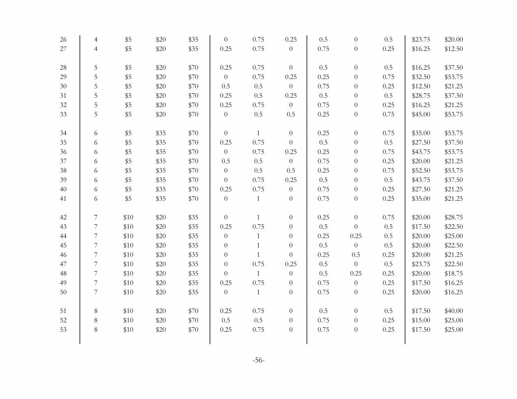
26 4 $5 $20 $35 0 0.75 0.25 0.5 0 0.5 $23.75 $20.0027 4 $5 $20 $35 0.25 0.75 0 0.75 0 0.25 $16.25 $12.50

28 5 $5 $20 $70 0.25 0.75 0 0.5 0 0.5 $16.25 $37.5029 5 $5 $20 $70 0 0.75 0.25 0.25 0 0.75 $32.50 $53.7530 5 $5 $20 $70 0.5 0.5 0 0.75 0 0.25 $12.50 $21.2531 5 $5 $20 $70 0.25 0.5 0.25 0.5 0 0.5 $28.75 $37.5032 5 $5 $20 $70 0.25 0.75 0 0.75 0 0.25 $16.25 $21.2533 5 $5 $20 $70 0 0.5 0.5 0.25 0 0.75 $45.00 $53.75

34 6 $5 $35 $70 0 1 0 0.25 0 0.75 $35.00 $53.7535 6 $5 $35 $70 0.25 0.75 0 0.5 0 0.5 $27.50 $37.5036 6 $5 $35 $70 0 0.75 0.25 0.25 0 0.75 $43.75 $53.7537 6 $5 $35 $70 0.5 0.5 0 0.75 0 0.25 $20.00 $21.2538 6 $5 $35 $70 0 0.5 0.5 0.25 0 0.75 $52.50 $53.7539 6 $5 $35 $70 0 0.75 0.25 0.5 0 0.5 $43.75 $37.5040 6 $5 $35 $70 0.25 0.75 0 0.75 0 0.25 $27.50 $21.2541 6 $5 $35 $70 0 1 0 0.75 0 0.25 $35.00 $21.25

42 7 $10 $20 $35 0 1 0 0.25 0 0.75 $20.00 $28.7543 7 $10 $20 $35 0.25 0.75 0 0.5 0 0.5 $17.50 $22.5044 7 $10 $20 $35 0 1 0 0.25 0.25 0.5 $20.00 $25.0045 7 $10 $20 $35 0 1 0 0.5 0 0.5 $20.00 $22.5046 7 $10 $20 $35 0 1 0 0.25 0.5 0.25 $20.00 $21.2547 7 $10 $20 $35 0 0.75 0.25 0.5 0 0.5 $23.75 $22.5048 7 $10 $20 $35 0 1 0 0.5 0.25 0.25 $20.00 $18.7549 7 $10 $20 $35 0.25 0.75 0 0.75 0 0.25 $17.50 $16.2550 7 $10 $20 $35 0 1 0 0.75 0 0.25 $20.00 $16.25

51 8 $10 $20 $70 0.25 0.75 0 0.5 0 0.5 $17.50 $40.0052 8 $10 $20 $70 0.5 0.5 0 0.75 0 0.25 $15.00 $25.0053 8 $10 $20 $70 0.25 0.75 0 0.75 0 0.25 $17.50 $25.00

-56-

54 9 $10 $35 $70 0 1 0 0.25 0 0.75 $35.00 $55.0055 9 $10 $35 $70 0.25 0.75 0 0.5 0 0.5 $28.75 $40.0056 9 $10 $35 $70 0 0.5 0.5 0.25 0 0.75 $52.50 $55.0057 9 $10 $35 $70 0 0.75 0.25 0.5 0 0.5 $43.75 $40.00

58 10 $20 $35 $70 0 1 0 0.25 0 0.75 $35.00 $57.5059 10 $20 $35 $70 0.25 0.75 0 0.5 0 0.5 $31.25 $45.0060 10 $20 $35 $70 0 0.75 0.25 0.25 0 0.75 $43.75 $57.5061 10 $20 $35 $70 0 1 0 0.5 0 0.5 $35.00 $45.0062 10 $20 $35 $70 0.5 0.5 0 0.75 0 0.25 $27.50 $32.5063 10 $20 $35 $70 0 1 0 0.25 0.5 0.25 $35.00 $40.0064 10 $20 $35 $70 0.25 0.5 0.25 0.5 0 0.5 $40.00 $45.0065 10 $20 $35 $70 0 0.5 0.5 0.25 0 0.75 $52.50 $57.5066 10 $20 $35 $70 0 1 0 0.5 0.25 0.25 $35.00 $36.2567 10 $20 $35 $70 0.25 0.75 0 0.75 0 0.25 $31.25 $32.5068 10 $20 $35 $70 0 0.75 0.25 0.5 0 0.5 $43.75 $45.0069 10 $20 $35 $70 0 1 0 0.75 0 0.25 $35.00 $32.50

-57-

Figure B1: Default Simple Lotteries

-58-

Table B2: Simple Lotteries vs. Compound Lotteries (Pairs 1-15)

Compound Lottery

Simple Lottery Initial Lottery Initial Lottery

Final Prizes Probabilities Prizes Probabilities “Double or Nothing” EV EV

Pair Context Low Middle High Low Middle High Low Middle High Low Middle High option Simple Compound

1 1 $0 $10 $20 0.5 0.5 0 $0 $10 $20 0.5 0.5 0 DON if middle $5.00 $5.00

2 1 $0 $10 $20 0 1 0 $0 $10 $20 0.5 0.5 0 DON if middle $10.00 $5.00

3 2 $0 $10 $35 0 1 0 $0 $5 $17.50 0 0.5 0.5 DON for any outcome $10.00 $11.254 2 $0 $10 $35 0.25 0.75 0 $0 $17.50 $35 0.5 0.5 0 DON if middle $7.50 $8.75

5 3 $0 $10 $70 0.25 0.75 0 $0 $35 $70 0 1 0 DON for any outcome $7.50 $35.00

6 3 $0 $10 $70 0 1 0 $0 $35 $70 0 1 0 DON for any outcome $10.00 $35.00

7 4 $0 $20 $35 0 1 0 $0 $10 $35 0 0.5 0.5 DON if middle $20.00 $22.50

8 4 $0 $20 $35 0 0.75 0.25 $0 $17.50 $35 0 0.5 0.5 DON if middle $23.75 $8.75

9 5 $0 $20 $70 0 0.5 0.5 $0 $35 $70 0 0.5 0.5 DON if middle $45.00 $52.50

10 5 $0 $20 $70 0.5 0 0.5 $0 $20 $35 0 0.5 0.5 DON if high $35.00 $27.50

11 5 $0 $20 $70 0 1 0 $0 $20 $35 0 0.5 0.5 DON if high $20.00 $27.50

12 5 $0 $20 $70 0 0.75 0.25 $0 $35 $70 0 0.5 0.5 DON if middle $32.50 $52.50

13 6 $0 $35 $70 0 1 0 $0 $35 $70 0 0.5 0.5 DON if middle $35.00 $52.50

14 6 $0 $35 $70 0 0.75 0.25 $0 $35 $70 0 1 0 DON for any outcome $43.75 $35.00

15 6 $0 $35 $70 0 0.75 0.25 $0 $35 $70 0 0.5 0.5 DON if middle $43.75 $52.50

-59-

Table B3: Simple Lotteries vs. Actuarially-Equivalent Lotteries (Pairs 16-30)

Simple Lottery Actuarially-Equivalent EV EV

Final Prizes Probabilities Lottery Probabilities Simple Actuarially-

Pair Context Low Middle High Low Middle High Low Middle High Equivalent

16 1 $0 $10 $20 0.5 0.5 0 0.75 0 0.25 $5.00 $5.00

17 1 $0 $10 $20 0 1 0 0.75 0 0.25 $10.00 $5.00

18 2 $0 $10 $35 0 1 0 0.5 0.25 0.25 $10.00 $11.25

19 2 $0 $10 $35 0.25 0.75 0 0.75 0 0.25 $7.50 $8.75

20 3 $0 $10 $70 0.25 0.75 0 0.5 0 0.5 $7.50 $35.00

21 3 $0 $10 $70 0 1 0 0.5 0 0.5 $10.00 $35.00

22 4 $0 $20 $35 0 1 0 0.25 0.25 0.5 $20.00 $22.50

23 4 $0 $20 $35 0 0.75 0.25 0.25 0 0.75 $23.75 $8.75

24 5 $0 $20 $70 0 0.5 0.5 0.25 0 0.75 $45.00 $52.50

25 5 $0 $20 $70 0.5 0 0.5 0.25 0.5 0.25 $35.00 $27.50

26 5 $0 $20 $70 0 1 0 0.25 0.5 0.25 $20.00 $27.50

27 5 $0 $20 $70 0 0.75 0.25 0.25 0 0.75 $32.50 $52.50

28 6 $0 $35 $70 0 1 0 0.25 0 0.75 $35.00 $52.50

29 6 $0 $35 $70 0 0.75 0.25 0.5 0 0.5 $43.75 $35.00

30 6 $0 $35 $70 0 0.75 0.25 0.25 0 0.75 $43.75 $52.50

-60-

Table B4: Actuarially-Equivalent Lotteries vs. Compound Lotteries (Pairs 31-40)

Compound Lottery

Actuarially-Equivalent Initial Lottery Initial Lottery EV EV

Final Prizes Lottery Probabilities Prizes Probabilities “Double or Nothing” Actuarially- Compound

Pair Context Low Middle High Low Middle High Low Middle High Low Middle High option Equivalent

31 1 $0 $10 $20 0.75 0 0.25 $0 $10 $20 0.5 0.5 0 DON if middle $5.00 $5.00

32 2 $0 $10 $35 0.5 0.25 0.25 $0 $5 $17.50 0 0.5 0.5 DON for any outcome $11.25 $11.2533 2 $0 $10 $35 0.75 0 0.25 $0 $17.50 $35 0.5 0.5 0 DON if middle $8.75 $8.75

34 3 $0 $10 $70 0.5 0 0.5 $0 $35 $70 0 1 0 DON for any outcome $35.00 $35.00

35 4 $0 $20 $35 0.25 0.25 0.5 $0 $10 $35 0 0.5 0.5 DON if middle $22.50 $22.50

36 4 $0 $20 $35 0.25 0 0.75 $0 $17.50 $35 0 0.5 0.5 DON if middle $8.75 $8.75

37 5 $0 $20 $70 0.25 0 0.75 $0 $35 $70 0 0.5 0.5 DON if middle $52.50 $52.50

48 5 $0 $20 $70 0.25 0.5 0.25 $0 $20 $35 0 0.5 0.5 DON if high $27.50 $27.50

30 6 $0 $35 $70 0.25 0 0.75 $0 $35 $70 0 0.5 0.5 DON if middle $52.50 $52.50

40 6 $0 $35 $70 0.5 0 0.5 $0 $35 $70 0 1 0 DON for any outcome $35.00 $35.00

-61-

Appendix C: Related Literature (NOT FOR PUBLICATION)

Cubitt, Starmer and Sugden [1998a] studied the Reduction of Compound Lotteries Axiom[ROCL] in a 1-in-1 design that gave each subject one and only one problem for real stakes and wasconceived to test principles of dynamic choice. Also, Starmer and Sugden [1991], Beattie andLoomes [1997] and Cubitt, Starmer and Sugden [1998] have studied the Random Lottery IncentiveMethod (RLIM), and as a by-product have tested the ROCL axiom. We focus on the results relatedto the ROCL axiom: Harrison and Swarthout [2011] review the results related to RLIM.

Cubitt, Starmer and Sugden [1998a] gave to one group of subjects one problem that involvedcompound lotteries and gave to another group the reduced compound version of the same problem.If ROCL is satisfied, one should see the same pattern of choice in both groups. They cannot findstatistically significant violations of ROCL in their design.

Starmer and Sugden [1991] gave their subjects two pairs of lotteries that were designed totest “common consequence” violations of EUT. In each pair i there was a risky (Ri) option and asafe (Si) option. They recruited 160 subjects that were divided into four groups of equal number.Two groups faced one of the two pairs in 1-in-1 treatments, while the other two groups were givenboth pairs to make a choice over using the RLIM to choose the pair for final payoff. We focus onthe latter two groups since RLIM induces four possible compound lotteries: i) (0.5, R1; 0.5, R2), ii)(0.5, R1; 0.5, S2), iii) (0.5, R2; 0.5, S1) and iv) (0.5, S1; 0.5, S2). The lottery parameters were chosento make compound lotteries ii) and iii) have equal actuarially-equivalent prospects.

They hypothesize that if a reduction principle holds, and if any of the induced compoundlotteries ii) and iii) above is preferred by a subject, then the other one must be preferred.30 Therejection of this hypothesis is a violation of ROCL, since this axiom implies that two compoundlotteries with the same actuarially-equivalent prospects should be equally preferred. Therefore, thenull hypothesis in Starmer and Sugden [1991; p. 976] is that “the choice between these tworesponses to be made at random; as a result, these responses should have the same expectedfrequency.” From the 80 subjects that faced the 1-in-2 treatments, 32.5% of the individuals chose(0.5, R1; 0.5, S2) and 15% chose (0.5, R2; 0.5, S1), thus Starmer and Sugden reject the nullhypothesis of equal frequency in choices based on a one-tail test with a binomial distribution andp-value=0.017. This pattern is very similar in each of the 1-in-2 treatments; in one of them theproportions are 30% and 15%, whereas in the other they are 35% and 15%. A two-sided FisherExact test yields a p-value of 0.934, which suggest that these patterns of choices are very similar inboth 1-in-2 treatments. Therefore, there is no statistical evidence to support ROCL in theirexperiment.

Beattie and Loomes [1997] examined 4 lottery choice tasks. The first 3 tasks involved abinary choice between two lotteries, and the fourth task involved the subject selecting one of fourpossible lotteries, two of which were compound lotteries.31 They recruited 289 subjects that were

30 Following Holt [1986], Starmer and Sugden [1991, p. 972] define the reduction principle to bewhen “compound lotteries are reduced to simple ones by the calculus of probabilities and that choices aredetermined by the subject’s preferences over such reduced lotteries.” This is what we call ROCL, in addition tosome axioms that are maintained for present purpose.

31 Beattie and Loomes [1997] use nine prospects: A= (0.2, £15; 0.8, £0), B= (0.25, £10; 0.75, £0), C=(0.8, £0; 0.2, £30), D= (0.8, £5; 0.2, £0), E=(0.8, £15; 0.2, £0), F = (1, £10), G=(1, £4), H=(0.5,£10; 0.5,£0),

-62-

randomly assigned to six groups. The first group faced a hypothetical treatment and was paid a flatfee for completing all four tasks. The second group was given a 1-in-4 treatment, and each of theother four groups faced one of the four tasks in 1-in-1 treatments. Sample sizes were 49 for thehypothetical treatment and the 1-in-4 treatment, and a total of 191 in the four 1-in-1 treatments.

Beattie and Loomes [1997; p. 164] find that “there is no support for the idea that twoproblems involving the same ‘reduced form’ alternatives – and therefore involving the samedifference between expected values – will be treated equivalently.” On this basis, their Question 3 inthe 1-in-4 treatment would be actuarially-equivalent to their Question 1 in the 1-in-1 treatment. Theyfound that the pattern of choices in both treatments are so different “that a chi-square test rejectswith a very great confidence (p<.001) the hypothesis that they are treated equivalently” (p. 164). Thep-value<0.001 of the Fisher Exact test provides further support for this violation of ROCL.

Their Question 4 is a task that is similar to the method developed by Binswanger [1980]:subjects are offered an ordered set of choices that increase the average payoff while increasingvariance. The difference with the Binswanger procedure is that two of the four choices involvedcompound lotteries: one paid a given amount of money if two Heads in a row were flipped, and theother paid a higher amount if three Heads in a row were flipped. For responses in Question 4,Beattie and Loomes [1997; p.162]

...conjecture that the REAL [1-in-1] treatment might stimulate the greatest effort topicture the full sequential process [of coin flipping in the compound prospects] and,as a part of that, to anticipate feelings at each stage in the sequence; whereas theHYPO [hypothetical] treatment would be most conducive to thinking of thealternatives in their reduced form as a set of simple lotteries... The RPSP [1-in-4treatment] might then, both formally and psychologically, represent an intermediateposition, making the process less readily imaginable by adding a further stage (therandom selection of the problem) to the beginning of the sequence, and reducing butnot eliminating the incentive to expend the necessary imaginative effort.

On this basis, they predict that, when answering Question 4, subjects in the hypothetical treatmentare more likely to think in reduced form probability distributions. Beattie and Loomes consider that thismight enhance the salience of the high-payoff option, and thus the compound lotteries are expectedto be chosen more frequently in the hypothetical treatment than in the 1-in-1 and 1-in-4 treatments.

Beattie and Loomes [1997; p.165] found support for these conjectures: Their subjects tendto choose the compound lotteries more often in the hypothetical treatment than in the ones witheconomic incentives (i.e., 1-in-1 and 1-in-4 treatments). They found that under the hypotheticaltreatment more than 1 in 3 of the sample opted for the compound lotteries; this proportion wasreduced in the 1-in-4 treatment to just over 1 in 5; and in the 1-in-1 treatment the proportion fell to1 in 12. A chi-square test rejects (p-value < 0.01) the hypothesis that there is no difference in

I=(£25 if two Heads in a row are flipped; otherwise nothing) and J=(£62.50 if three Heads in a row areflipped; otherwise nothing). Questions 1 through 3 are binary choices that offer, respectively, A or B, C or Dand E or F. In Question 4, the subject must choose the prospect that she prefers the most among G, H, I orJ. Options I and J are compound lotteries with 2 and 3 stages, respectively.

-63-

patterns across treatments. The Fisher Exact test is consistent with this result.32

Cubitt, Starmer and Sugden [1998] use common consequence and common ratio pairs ofpairs in three experiments. We focus in the first two since the third experiment has no treatmentsrelevant to test ROCL. In the first experiment they compare 1-in-1 choices with 1-in-2 choices.Their comparison rests on subjects not having extreme risk-loving preferences over the pairs oflotteries in the 1-in-2 treatment designed to capture this behavior. Given that this a priori assumptionis true, and it is generally supported by their data, the lottery pairs in each of the 1-in-2 treatmentswere chosen to generate compound prospects with actuarially-equivalent lotteries equal to theprospects in each of the 1-in-1 treatments.

If ROCL is satisfied, the distribution of responses between risky and safe lotteries should bethe same in both treatments. The p-value from the Fisher Exact test in one of the 1-in-1 and 1-in-2treatment comparisons33 is 0.14, which suggests that ROCL is most likely violated.34

Similarly, in the second experiment the 1-in-2 treatment induced compound lotteries withactuarially-equivalent prospects equal to the lottery choices in one of their 1-in-1 treatment. In thelatter, 52% of the 46 subjects chose the risky lottery, whereas 38% of the 53 subjects in the 1-in-2treatment chose the risky prospect. These choice patterns suggest that ROCL does not hold in thesecond experiment.35

32 We test the similarity between treatments of the proportions of subjects that chose each of the fourprospects in Question 4. The two-sided Fisher Exact test applied to the hypothetical and the 1-in-1 treatmentsrejects the hypothesis of no difference in choice patterns (p-value = 0.001). The p-value for the comparison ofthe same four choices between the hypothetical and the 1-in-4 treatments is 0.473.

33 Groups 1.1 and 1.3 in their notation.34 The proportions of subjects that chose the risky prospect in the other 1-in-1 and 1-in-2 treatments

(groups 1.2 and 1.4 in their notation) are close: 50% and 55%, respectively. However, we cannot perform theFisher Exact test for this 1-in-1 and 1-in-2 comparison, since the compound lotteries induced by the 1-in-2treatment have actuarially-equivalent prospects equal to the ones in the 1-in-1 treatment only if the subjectsdo not exhibit extreme risk-loving preferences. Since 8% of the subjects in this 1-in-2 treatment exhibitedrisk-loving preferences, one cannot perform the Fisher test because this contaminates the comparisonbetween the compound lotteries and their actuarially-equivalent counterparts.

35 Since one of the subjects in the 1-in-2 treatment (group 2.3) exhibited risk-loving preferences, wecannot perform the Fisher Exact test for the reasons explained earlier.

-64-

Appendix D: Nonparametric Tests (NOT FOR PUBLICATION)

A. Choice Patterns Where ROCL Predicts Indifference

Research Hypothesis: Subjects are indifferent between a compound (C) lottery and its pairedactuarially-equivalent (AE) lottery, and therefore the choice between both lotteries is made atrandom in any of our 10 AE-C pairs in Table B4. As a result we should observe equiprobableresponse proportions between C and AE lotteries. ROCL is rejected if we can provide statisticalevidence that the proportion of observations in which subjects chose a C lottery over its AE lotteryis different from the proportion of choices in which subjects chose the AE lottery over the C lottery.

Structure of data sets: We analyze the observed responses from subjects who were presentedwith any of the 10 pairs described in Table B4 and which contain both a C lottery and its AE lottery.First, we study the responses from 32 subjects who were presented with one and only one of theAE-C pairs in 1-in-1 treatment. We also study the 620 responses from the 62 subjects that werepresented with all of the 10 AE-C pairs in the 1-in-40 treatment. In terms of the statistical literature,the responses to each of the AE-C pairs in the 1-in-1 constitute an “independent” sample. Thismeans that subjects are presented with one and only one choice, thus one observation does notaffect any other observation in the sample. Conversely, the responses to the AE-C pairs in the 1-in-40 constitute 10 “dependent” samples since each of the 62 subjects responded to each of the 10 AE-C pairs.

We analyze the data separately because, in contrast to the 1-in-40 treatment which uses therandom lottery incentive mechanism (RLIM) as payment protocol, any conclusion drawn from the1-in-1 treatment does not depend in the independence axiom assumed by the RLIM. We want tocontrol for the possibility that the observed choice patterns in the 1-in-40 treatment are affected bythis payment protocol. This means that any failure to see indifference between a C lottery and itsand AE lottery in our data could be explained by confounds created by the payment protocol. Byanalyzing data from the 1-in-1 treatment only, we avoid possible confounds created by the RLIM.

1-in-1 Treatment

We apply the Binomial probability test to each of the AE-C pair for which there is sufficientdata to conduct the test. The latter allows us to test individually for each AE-C pair if subjectschoose the C lottery and the AE lottery in equal proportions. We also use a generalized version ofthe Fisher Exact test that allows us to jointly test the statistical null hypothesis that the proportionsof subjects that chose the C lottery over the AE lottery in each of the AE-C lottery pairs are thesame. Both test can provide statistical evidence of the overall performance of the ROCLindifference prediction.

Statistical Null Hypothesis of the Binomial Probability Test: For a given AE-C lottery pair, theproportion of subjects that choose the C lottery is 50 %. This is equivalent to test the claim thatsubjects choose the AE lottery and the C lottery in equal proportions when they are presented with agiven AE-C lotteries.

If this statistical null hypothesis is not rejected then we conclude that there is evidence tosupport the claim that, for a given AE-C pair, subjects choose the AE and the C lotteries in equal

-65-

proportions. If the null hypothesis of the test is rejected, then we concluded that subjects choose theAE and the C lotteries in different proportions. The rejection (acceptance) of the statistical nullhypothesis implies that the research hypothesis is rejected (accepted) and we conclude that there isevidence to support the claim that the basic ROCL indifference prediction is violated (satisfied) in agiven AE-C pair.

This is an appropriate test to use for this treatment because it allows us to test the equality ofproportions implied by the ROCL prediction. More importantly, the basic assumptions of the testare satisfied by the data. As described by Sheskin[2004; p. 245], the assumptions are: (i) each of the nobservations are independent (i.e., the outcome of one observation is not affected by the outcomeof another observation), (ii) each observation is randomly selected from a population, and (iii) eachobservation can be classified only two into mutually exclusive categories. Assumption (i) is satisfiedbecause each subject makes one and only one choice. Assumption (ii) is also satisfied because eachsubject is randomly recruited from the extensive subject pool of the EXCEN laboratory at GeorgiaState University. Finally (iii) is also satisfied because subjects can only choose either the C lottery orthe AE lottery in each of the 10 AE-C pairs.

Statistical Null Hypothesis of the Generalized Fisher Exact Test: The proportion of individualschoosing the C lotteries is the same for all the AE-C lottery pairs.

The contingency table used in the test has the following structure:

Choice

Pair AE Lottery C Lottery Total

AE-C pair 1 n11 n12 n11 + n12

AE-C pair 2 n21 n22 n21 + n22

. . . .

AE-C pair r nr1 nr2 nr1 + nr2

Total 'i-1,2,...,r (ni1) 'i-1,2,...,r (ni2) 'i-1,2,...,r (ni1+ni2)

The number in each cell is defined as follows. The symbol n11 represents the number ofindividuals that chose the AE lottery when they were presented with the AE-C lottery pair 1. Thesymbol n12 represents the number of individuals that chose the C lottery when they were presentedwith the same AE-C pair 1. The sum n11+n12 represents the total number of subjects that werepresented with the AE-C lottery pair 1. The interpretation of ni1 and ni2, for i=2, 3, ..., r, can besimilarly derived. The generalized Fisher Exact test tests the null hypothesis that the proportion ofsubjects that choose the C lottery is statistically the same for all of the r AE-C lottery pairs used inthe table. Formally, the statistical null hypothesis is Ho: p1 = p2= ... =pr,, where pi = ni2 /(ni1 +ni2) for i=1, 2, 3, ..., r.

We use this test in conjunction with the Binomial probability test applied individually toeach of the AE-C lottery pairs to make stronger claims of the overall performance of ROCL. If the

-66-

Binomial probability test does not reject its statistical null hypothesis for each of the AE-C lotterypairs and if the statistical null hypothesis of the generalized Fisher Exact test is not rejected, we canconclude that the proportion of subjects that chose the C lottery is statistically the same for all AE-Cand therefore the ROCL indifference prediction is supported. If we can reject the statistical nullhypothesis of the generalized Fisher Exact test, we can conclude that at least in two of the AE-Cpairs the proportions of subjects that chose the C lottery are different. For example, suppose therewere only 2 AE-C lottery pairs. If the Fisher Exact test rejects the null hypothesis, we conclude thatthe proportions of subjects choosing the C lottery are not the same in the two lottery pairs.Therefore, even if one of the proportions was equal to 50%, as ROCL predicts for any given AE-Clottery pair, the rejection of the statistical null would imply that the other proportion is notstatistically equal to 50%. Consequently, we would reject the research hypothesis that subjects satisfyROCL and choose at random between the AE and the C lottery in all of the AE-C lottery pairs.

The generalized Fisher Exact test is appropriate to test the joint hypothesis that theproportion of subjects that chose the C lottery is the same in all of the AE-C lottery pairs. The basicassumptions of the test are satisfied by the data. As described by Sheskin[2004; p. 424 and 506], theassumptions are: (i) each of the n observations are independent (i.e., the outcome of oneobservation is not affected by the outcome of another observation), (ii) each observation israndomly selected from a population, (iii) each observation can be classified only into mutuallyexclusive categories, (iv) the Fisher Exact test is recommended when the size of the sample is small,and (v) many sources note that an additional assumption is that the sum of the rows and columns ofthe contingency table used in the Fisher Exact test are predetermined by the researcher.Assumptions (i)-(iii) are satisfied for the same reasons we explained in the Binomial probability test.The Fisher Exact test is commonly used for small samples like ours instead of the Chi-square test ofhomogeneity, which relies on large samples to work appropriately. Finally, the last assumption is notmet by our data, however, Sheskin [2004; p. 506] claim that this is rarely met in practice and,consequently, the test is used in contingency tables when “one or neither of the marginal sums isdetermined by the researcher.”

1-in-40 Treatment

The strategy to test the basic prediction of indifference in the “Pay-1-in-40 compound isdifferent from the one used in the “Pay-1-in-1-compound.” The reason is that the structure of thedata in each of the treatments is different. In the case of the 1-in-1 treatment, each of the 10 AE-Clottery pairs generated, using the terminology of the statistical literature, an “independent” sample inthe sense that there was no subject that made choices over more than one AE-C lottery pair. On thecontrary, in the 1-in-40 treatment we have multiple “dependent” samples. This means that severalsubjects made choices over each of our 10 AE-C lottery pairs, and therefore, we obtain 10“dependent” samples. This subtle difference has relevant implications for the type of nonparametrictest that one should use to test any hypothesis with the structure of the data we described. We usethe Cochran Q test to test the basic ROCL prediction of indifference in the 1-in-40 treatment.

Statistical Null Hypothesis of the Cochran Q Test: The proportion of subjects that choose the C isthe same in each of the 10 AE-C lottery pairs.

The information needed to perform this test is captured in a table of the following type:

-67-

AE-C pair 1 AE-C pair 2 . AE-C pair 9 AE-C pair 10

Subject 1 c1-1 c1-2 . c1-9 c1-10

Subject 2 c2-1 c2-2 . c2-9 c2-10

. . . . .

Subject n cn-1 cn-2 . cn-9 cn-10

Total 'i-1,2,...,n (ci-1) 'i-1,2,...,n (ci-2) . 'i-1,2,...,n (ci-9) 'i-1,2,...,r (ci-10)

The number in each cell is defined as follows. The symbol c1-1 is a dichotomous variable thatcan be either 0 or 1 and records the choice that was made when of subject 1 was presented with theAE-C lottery pairs. If subject 1 chooses the AE lottery, c1-1 is equal to 0; but if the subject choosesthe C lottery instead, c1-1 is equal to 1. the represents the number of individuals that chose the AElottery when they were presented with the AE-C lottery pair 1. The symbols c1-2, c1-3,... and c1-10, aresimilarly defined and record subject 1's choices in AE-C pairs 2 through 10. Similarly, the symbols ci-

1, ci-2,... and ci-10 record the choices that subject i made in each of the 10 AE-C lottery pairs. The sum'i-1,2,...,n (ci-k) represents the total number of subjects, out of the n subjects, that chose the C lotterywhen they were presented with the AE-C lottery pair j. The Cochran Q test tests if the proportion ofsubjects that chose the C lottery in each of the 10 AE-C lottery pairs are the same. Thus thestatistical null hypothesis is Ho: p1 = p2= ... =p10,, where pi = 'i-1,2,...,n (ci-k) /n for i=1, 2, 3, ..., 10. Theactual statistic of the Cochran Q test involves information of these proportions, as well asinformation per subject.

This joint hypothesis is enough to reject the indifference prediction. For example, supposethere were only 2 AE-C lottery pairs. If the Cochran Q test rejects the null hypothesis, we concludethat the proportions of subjects choosing the C lottery are not the same in the two lottery pairs.Therefore, even if one of the proportions is equal to 50% as ROCL predicted, the test providesevidence that the other proportion is not equal to 50%. Consequently, we would reject the researchhypothesis that subjects satisfy ROCL and choose at random between the AE and the C lottery inany of the AE-C lottery pairs. In the text we provide confidence intervals36 on the number ofsubjects (out of the 62 in our sample) that chose the S lottery in each of the AE-C lottery. If for agiven AE-C lottery pair the number 31 is not contained in the confidence interval, it implies thatwith 95% probability the proportion of the 62 subjects that chose the C lottery will not be 50%. Wecould have apply the Binomial probability test to each of the 10 AE-C pairs in the 1-in-40 treatment.However, this would not be appropriate since the Binomial test assumes “independence” in thesample in the statistical sense which is not satisfied in the present treatment.

The Cochran Q test is an appropriate test in this treatment because it allows us to jointlyreject the null hypothesis that subjects choose the C lottery and the AE lottery in equal proportionswhen the data set is composed by multiple dependent samples. The basic assumptions of the test aresatisfied by the data. As described by Sheskin[2004; p. 245], the assumptions are: (i) each of thesubjects respond to each of the 10 AE-C lottery pairs, (ii) one has to control for order effects and (iii) each observation can be classified only into mutually exclusive categories. Assumptions (i) is

36 We use the -total- Stata command to calculate the confidence intervals.

-68-

satisfied since in the 1-in-40 treatment each subjects respond to all 40 lottery pairs, which include the10 AE-C pairs. Assumption (ii) is also satisfied because in our experiments each subject is presentedwith the 40 lotteries in random order. Assumption (iii) is trivially satisfied since in each of the AE-Cpairs the subjects have to make a dichotomous choice.

B. Choice Patterns Where ROCL Predicts Consistent Choices

Research Null Hypothesis: Subjects choose the S lottery when presented with the S-C lotterypair if and only if they also choose the S lottery when presented with the corresponding S-AE lotterypair. This is equivalent to state the null hypothesis using the C and AE lotteries but we chose towork with the S lottery for simplicity. Therefore, ROCL is satisfied if we can provide statisticalevidence that the proportion of subjects that choose the S lottery when presented with a S-C pair isequal to the proportion of subjects that choose also the S lottery when presented with the paired S-AE pair.

Structure of data sets: We use data from the 62 subjects in the 1-in-40 treatment who werepresented with each of the 30 lottery pairs in Tables B2 and B3. Each of the 15 S-C lottery pairs inTable B2 has a corresponding S-AE pair in Table B3. Therefore, we can construct 15 comparisonsof pairs that constitute 15 consistency tests of ROCL. In the 1-in-40 we again have to assume thatthe independence axiom holds. Therefore, we also use data from the 1-in-1 treatment to control forpossible confounds created by the RLIM. However, we have to assume homogeneity in riskpreferences for the analysis of this particular treatment. The reason is that the response of anysubject to a particular S-C lottery pair, is going to be compared with the response of another subjectto the paired S-AE lottery pair. In terms of the statistical literature, the responses to each of the S-Cor S-AE pairs in the 1-in-1 constitute an “independent” sample. Conversely, the responses to eachof the S-C or S-AE pairs in the 1-in-40 constitute 30 “dependent” samples since each of the 62subjects responded to each of the 15 S-C and the 15 S-AE. Also, each of the 15 comparisons isconstructed by matching a S-C pair with its corresponding S-AE pair.

Analysis of data from the 1-in-1 treatment

We use the Fisher Exact test to evaluate the consistency predicted by ROCL in each of thepaired comparisons of S-C pairs and S-AE pairs for which we have enough data to conduct the test.We also use the Cochran-Mantel-Haenszel (CMH) as a joint test of the 15 paired comparisons toevaluate the overall performance of the ROCL consistency prediction.

Statistical Null Hypothesis of the Fisher Exact Test: For any given paired comparison, subjectschoose the S lottery in the same proportion when presented with a S-C pair and with itscorresponding S-AE lottery pair.

The table shows statistical tests on contingency tables of the following form:

-69-

Choice

S AE/C Total

S-AE pair a b a+b

S-C pair c d c+d

Total a+c b+d a+b+c+d

The positions in each cell are defined as follows. The letter a represents the number ofindividuals that chose the simple lottery when they were presented with a S-AE pair. The letter crepresents the number of individuals that chose the simple lottery when they were presented withthe corresponding S-C pair. The letter b represents the number of subjects that chose the AE lotterywhen they were presented with the S-AE lottery pair. Similarly, the letter d represents the number ofsubjects that chose the C lottery when they were presented with the corresponding S-C lottery pair.In the notation of the previous note, the proportions used in the Fisher Exact test are defined as π1

= a/(a+b) and π2 =c/(c+d).

The Fisher Exact test for 2 × 2 contingency tables is appropriate to test individually in eachof the 15 matched pairs the hypothesis that the proportion of subjects that chose the S lottery is thesame when they are presented with the S-C or its corresponding S-AE pair. The basic assumptionsof the test are satisfied by the data. As described by Sheskin[2004; p. 424 and 506], the assumptionsare: (i) each of the n observations are independent (i.e., the outcome of one observation is notaffected by the outcome of another observation), (ii) each observation is randomly selected from apopulation, (iii) each observation can be classified only into mutually exclusive categories, (iv) theFisher Exact test is recommended when the size of the sample is small, and (v) many sources notethat an additional assumption is that the sum of the rows and columns of the contingency table usedin the Fisher Exact test are predetermined by the researcher. Assumptions (i)-(iv) are satisfied for thesame reasons we explained in the in the case of the generalized Fisher exact test. Finally, as weexplained before assumption (v) is not satisfied in our data.

Statistical Null Hypothesis of the Cochran-Mantel-Haenszel test: In all of the 15 paired comparisonssubjects choose in the same proportion the S lottery when presented with the S-C lottery pair and itspaired S-AE lottery pairs. More formally, the odds ratio of each of the 15 contingency tablesconstructed from the 15 paired comparisons are jointly equal to 1.

If the CMH test rejects the null hypothesis, then we interpret this as evidence of ROCL-inconsistent observed behavior. However, if we cannot reject the null, we conclude that subjectsmake choices according to the ROCL consistency predictions in the 15 pair comparisons even if wefind that the Fisher Exact tests rejects its null hypothesis for some of the paired comparisons.

The CMH is the appropriate joint test to apply since it allows us to pool the data of multiplecontingency tables that satisfy the assumptions needed for the Fisher Exact test and test jointly thehomogeneity of the tables.

-70-

Analysis of data from the 1-in-40 treatment

We use the Cochran Q test coupled with the Bonferroni-Dunn (B-D) method to test thestatistical hypothesis that subjects choose the S lottery in the same proportion when presented with aS-C lottery pair and with the corresponding S-AE lottery pair. The B-D method allows us to test if,in each of the 15 paired comparisons of S-C and S-AE lottery pairs, the observed difference in theproportion of subjects that chose the S lottery is statistically significant.

The B-D method is a post-hoc procedure that is conducted after calculating the Cochran Qtest. The first step is to conduct the latter test to reject or not reject the null hypothesis that theproportions of individuals that choose the S lottery are the same in all 15 S-C and 15 S-AE lotterypairs. If this null is rejected the B-D method involves calculating a critical value d (see Sheskin[2004;p. 871] for the definition) that allows to evaluate the statistical significance of the difference inproportions and that takes into account all the information of the 30 lottery pairs and a confidencelevel of α.

Statistical Null Hypothesis in each of the Pair Comparisons using the B-D method: Define p1 as theproportion of subjects that choose the S lottery when presented with a given S-AE lottery pair.Similarly, define p2 as the proportion of subjects that chose the S lottery in the paired S-C lotterypair. The statistical null hypothesis is that, for a given paired comparison, p1=p2.

The B-D method rejects the statistical null hypothesis if |p1-p2|> d. In this case we wouldconclude that the observed difference in proportions in a given paired comparison is statisticallysignificant. This is a more powerful test than conducting individual tests for each paired comparisonbecause the critical value d takes into account the information of all of the 15 comparisons. SeeSheskin [2004; p. 871] for further details of the B-D method.

The Cochran Q test coupled with the B-D method are appropriate to test in this treatmentthe null hypothesis that subjects choose the S lottery in the same proportion when presented with agiven S-C pair and with its corresponding S-AE lottery, and the data set is composed by multipledependent samples in the sense we explained above. The basic assumptions of the Cochran Q testare satisfied by the data. As described by Sheskin[2004; p. 245], the assumptions are: (i) each of thesubjects respond to each of the 15 S-C lottery pairs and the 15 S-AE lottery pairs, (ii) one has tocontrol for order effects and (iii) each observation can be classified only into mutually exclusivecategories. Assumptions (i) is satisfied since in the 1-in-40 treatment each subjects respond to all 40lottery pairs, which include the 15 S-C pairs and the 15 S-AE pairs. Assumption (ii) is also satisfiedbecause in our experiments each subject is presented with the 40 lotteries in random order.Assumption (iii) is trivially satisfied since in each of the AE-C pairs the subjects have to make adichotomous choice. The B-D method applied to the Cochran Q test does not require any extraassumptions. However, the calculation of the critical value to make the comparisons requires todefine a family wise Type I error rate (αFW). Sheskin [2004; p. 871] claims that “[w]hen a limitednumber of comparisons are planned prior to collecting the data, most sources take the position thata researcher is not obliged to control the value of αFW . In such a case, the per comparison Type Ierror rate (αPC) will be equal to the prespecified value of alpha [the confidence level].”

We are also interested in studying the patterns in the violation of ROCL. We want to test thestatistical validity of differences in switching behavior. A pattern inconsistent with ROCL would be

-71-

subjects choosing the S lottery when presented with a given S-C lottery pair, but switching to preferthe AE lottery when presented with the matched S-AE pair. We construct 2 × 2 contingency tablesthat show the number of subjects in any given matched pair who exhibit each of the four possiblechoice patterns: (i) always choosing the S lottery; (ii) choosing the S lottery when presented with a S-C pair and switching to prefer the AE lottery when presented with the matched S-AE pair; (iii)choosing the C lottery when presented with a S-C pair and switching to prefer the S lottery whenpresented with the matched S-AE; and (iv) choosing the C lottery when presented with the S-Clottery and preferring the AE lottery when presented with the matched S-AE. We use the McNemartest to evaluate the statistical significance of patterns in the violations of ROCL.

Statistical Null Hypothesis of the McNemar Test: Subjects exhibit the discordant choice patterns(ii) and (iii) in equal proportions within each set of matched pairs.

If the statistical null hypothesis is rejected then we can claim that there is an statisticaldifference in the two possible patterns of switching behavior that violate ROCL.

The test requires to construct a contingency tables of the following form:

Simple Lottery vs. Actuarially-Equivalent

LeftLottery

RightLottery

Total

Simple Lottery vs.

Compound Lottery

Left lottery a b a+b

Right lottery c d c+d

Total a+c b+d a+b+c+d

The positions in each cell are defined as follows. The letter a represents the number ofindividuals that chose the left lottery both when they were presented with a pair of a simple lotteryand a compound lottery (S-C) and a corresponding pair that has the same simple lottery and theactuarially-equivalent lottery (S-AE) of the compound lottery. The simple lotteries, and therefore thecompound and their actuarially equivalent lotteries, are always in the same position across. For thepurpose of the statistical tests, the simple lotteries are always the left lotteries; the compound andtheir actuarially-equivalent lotteries are always the right lotteries. Therefore, a is the number ofindividuals that chose the simple lottery when the were presented with a given pair of S-C and itscorresponding pair of S-AE. The letter c represents the number of individuals that chose the simplelottery when they were presented with a given pair of S-AE but that chose the compound lotterywhen they were presented with corresponding pair of S-C.

The McNemar test is an appropriate test to apply in this context. The assumptions of the testare (See Sheskin [2004; pp. 634]): (i) the sample of n subjects has been randomly selected from thepopulation, (ii) each of the n onservations in the contingency table is independent of other

-72-

observations, (iii) each observation can be classified only into mutually exclusive categories, and (iv)the test should not be used with extremely small samples. Assumptions (i) and (iii) are satisfied forreasons we explained before. Even though there is no agreement of what an small sample is for theMcNemar test, we follow the recommendation of the literature and provide in our results the exactprobability of the test. Assumption (ii) is not satisfied since each subject respond makes choice overmore than one pair. However, the test still allows us to draw conclusions about the discordantswitching patterns but does not allow to make causal inferences, which is enough for our purposes.In fact it will allows us to conclude if there is an statistical difference between the two possiblechoice patterns that contradict ROCL Nevertheless, it will not allow us to conclude anything aboutthe source of this difference (see Sheskin [2004; p. 639]).

-73-

Appendix E: Additional Econometric Analysis (NOT FOR PUBLICATION)

Analysis of Data from the 1-in-1 Treatment.

Assuming homogeneity in preferences, we find that the model that best describes the data isthe one that allows for the source-dependent version of RDU, and conditional on this model there isno evidence of violations of ROCL. Both the Vuong test and the Clarke test provide statisticalevidence that the model that allows for the source-dependent version of the RDU is the best modelto explain the data in the 1-in-1 treatment.37 Table E1 shows the parameter estimates of the twomodels we consider. In particular, panel A shows the estimates for the model that allows for thesource-dependent version of RDU. We find that the estimates for parameters r, rc, γ and γc are 0.62,0.14, 0.77 and -0.19, respectively. A test of the joint null hypothesis that rc = γc = 0 results in a p-value of .29. This implies that there is no statistical evidence for source-dependency both in theutility and the probability weighting functions, and therefore no evidence of violations of ROCLwhen homogeneity is assumed. If we had assumed that subjects behave according to the source-dependent EUT, we would have incorrectly concluded that there is evidence of violations of ROCLas suggested by the estimate of rc equal to 0.27 which has a p-value of 0.008 (see panel B of TableE1). A joint test of r and rc results in a p-value less than 0.0001. This highlights the importance ofchoosing the preference representation that best characterizes the way in which individuals makechoices.

Although the model that best characterizes behavior in the 1-in-1 treatment is the source-dependent version of the RDU model, there is evidence of marginal diminishing returns but noevidence of probability weighting.38 The parameter estimates for r and γ are equal to 0.62 and 0.77.Figure E1 shows the functions implied by these estimates and are plotted in the relevant domains. Atest for the hypothesis that γ=1 results in a p-value of 0.23, which provides no evidence ofprobability weighting.

Analysis of Data from the 1-in-40 Treatment.

Assuming homogeneity , we find that the model that best describes the data is the one thatallows for the source-dependence version of RDU, and conditional on this model we find evidenceof violations of ROCL. Both the Vuong test and the Clarke test provide evidence to support thesource-dependent RDU as the best model to explain the data in the 1-in-40 treatment.39 An statisticaltest for the joint null hypothesis that rc = γc=0 results in a p-value less than 0.0001.

The estimates for r, rc, γ and γc are 0.57, 0.11, 1.09 and -0.40, respectively. This implies thatthe nature of the violation has two components. First, the estimates suggests that when a typical

37 When we assume homogeneity in risk attitudes, the Vuong test statistic is -1.45 in favor of thesource-dependent RDU, with a p-value of .073. Further, the Clarke test also gives evidence in favor of thesource-dependent RDU with a test statistic equal to 44.

38 The Vuong and the Clarke tests provide evidence to choose the model that bests characterize databetween two models but are agnostic about the statistical significance of the winning model.

39 When we assume homogeneity in risk attitudes, the Vuong test statistic is -5.16 in favor of thesource-dependent RDU, with a p-value less than 0.001. Further, the Clarke test also gives evidence in favor ofthe source-dependent RDU with a test statistic equal to 935.

-74-

individual is presented with a compound lottery he behaves as if the utility function was moreconcave. The linear combination of parameters r + rc results in an estimated coefficient of 0.68 witha p-value less than 0.0001 and a test of the null hypothesis of r + rc = 0.57 results in a p-value equalto 0.0001. Thus a typical subject would increase his utility risk aversion parameter from 0.57 to 0.68when presented with a compound lottery. Second, there is no evidence of probability weightingwhen subjects are presented with simple lotteries but there is evidence of probability optimism whensubjects evaluate compound lotteries. A test on the probability weighting parameter for γ = 1 resultsin a p-value equal to 0.28 and the linear combination γ + γc results in an estimated parameter equalto 0.69 with a p-value less than 0.001. Hence, when presented with a simple lottery a typical subjectdisplays no probability weighting but does exhibits diminishing marginal returns; however, whenfacing a compound lottery, a typical subject behaves as if the utility function was more concave andthe probability weighting function displays probability optimism. Figure E2 shows how theconcavity of the utility function and the probability weighting function differ when individuals arepresented with a simple or a compound lottery.

-75-

Table E1: Estimates of Source-Dependent RDU and EUT Model Allowing for

Heterogeneity

Data from the 1-in-1 treatment (N=133). Estimates from the Fechner error parameter omitted

A. Source-Dependent RDU(LL=-81.82)

| Coef. Std. Err. z P>|z| [95% Conf. Interval]-------------+----------------------------------------------------------------r | .6182909 .0669022 9.24 0.000 .4871649 .7494169 |r_rocl | .1410226 .0922965 1.53 0.127 -.0398752 .3219204 |γ | .7699848 .193429 3.98 0.000 .3908708 1.149099 |γc | -.1955013 .1819329 -1.07 0.283 -.5520832 .1610806

(Ho: rc = γc = 0; p-value = 0.2848)

(Ho: r = γ = 0; p-value < 0.0001)

B. Source-Dependent Version of EUT (LL=-84.24)

| Robust | Coef. Std. Err. z P>|z| [95% Conf. Interval]-------------+----------------------------------------------------------------r | .5799532 .0731694 7.93 0.000 .4365438 .7233626 |rc | .2717936 .1028005 2.64 0.008 .0703083 .4732789

(Ho: r=rc=0; p-value < 0.0001)

-76-

Figure E1: Estimated Functions from the RDU Specification in the 1-in-1 TreatmentAssuming Homogeneity in Preferences

-77-

Table E2: Estimates of Source-Dependent RDU and EUT Model Allowing for

Heterogeneity

Data from the 1-in-40 treatment (N=2480= 62 Subjects × 40 choices). Estimates from the Fechner

error parameter omitted

A. Source-Dependent RDU (LL=-1460.57)

| Robust | Coef. Std. Err. z P>|z| [95% Conf. Interval]-------------+----------------------------------------------------------------r | .5670508 .024286 23.35 0.000 .519451 .6146505 |rc | .1090157 .0231279 4.71 0.000 .0636858 .1543456 |γ | 1.088315 .081601 13.34 0.000 .9283802 1.24825 |γc | -.3957716 .0587485 -6.74 0.000 -.5109165 -.2806266

(Ho: rc = γc = 0; p-value<0.0001)(Ho: r = γ = 0; p-value=0.0001)

B. Version of EUT (LL=-1512.45)

| Robust | Coef. Std. Err. z P>|z| [95% Conf. Interval]-------------+----------------------------------------------------------------r | .5906296 .0352857 16.74 0.000 .5214708 .6597883 |rc | -.0071859 .0194071 -0.37 0.711 -.0452233 .0308514

-78-

Figure E2: Estimated Functions from the RDU Specification in the 1-in-40 TreatmentAssuming Homogeneity in Preferences

-79-

Appendix F: Detailed Binomial Test Results (NOT FOR PUBLICATION)

The following tests are conducted over the actuarially-equivalent and compound lottery pairsin Table B4 (Pairs 31-40).

Binomial tests for treatment 1-in-1: We do not report the test for pairs 31, 35 and 35 because for thefirst one there was only one observation and for the last two there were no observations at all.

Note: In the following Binomial tests “N” is the total size of the sample for each lottery pair and“Observed k” is the number of subjects (out of the N subjects) that chose the compound lottery.

Pair 32

Variable | N Observed k Expected k Assumed p Observed p-------------+------------------------------------------------------------choice_aed~2 | 3 3 1.5 0.50000 1.00000

Pr(k >= 3) = 0.125000 (one-sided test) Pr(k <= 3) = 1.000000 (one-sided test) Pr(k <= 0 or k >= 3) = 0.250000 (two-sided test)

Pair 33

Variable | N Observed k Expected k Assumed p Observed p-------------+------------------------------------------------------------choice_aed~3 | 7 5 3.5 0.50000 0.71429

Pr(k >= 5) = 0.226563 (one-sided test) Pr(k <= 5) = 0.937500 (one-sided test) Pr(k <= 2 or k >= 5) = 0.453125 (two-sided test)

Pair 36

Variable | N Observed k Expected k Assumed p Observed p-------------+------------------------------------------------------------choice_aed~6 | 5 1 2.5 0.50000 0.20000

Pr(k >= 1) = 0.968750 (one-sided test) Pr(k <= 1) = 0.187500 (one-sided test) Pr(k <= 1 or k >= 4) = 0.375000 (two-sided test)

Pair 37

Variable | N Observed k Expected k Assumed p Observed p-------------+------------------------------------------------------------choice_aed~7 | 2 1 1 0.50000 0.50000

Pr(k >= 1) = 0.750000 (one-sided test) Pr(k <= 1) = 0.750000 (one-sided test) Pr(k <= 1 or k >= 1) = 1.000000 (two-sided test)

Pair 38

-80-

Variable | N Observed k Expected k Assumed p Observed p-------------+------------------------------------------------------------choice_aed~8 | 3 1 1.5 0.50000 0.33333

Pr(k >= 1) = 0.875000 (one-sided test) Pr(k <= 1) = 0.500000 (one-sided test) Pr(k <= 1 or k >= 2) = 1.000000 (two-sided test)

Pair 39

Variable | N Observed k Expected k Assumed p Observed p-------------+------------------------------------------------------------choice_aed~9 | 5 4 2.5 0.50000 0.80000

Pr(k >= 4) = 0.187500 (one-sided test) Pr(k <= 4) = 0.968750 (one-sided test) Pr(k <= 1 or k >= 4) = 0.375000 (two-sided test)

Pair 40

Variable | N Observed k Expected k Assumed p Observed p-------------+------------------------------------------------------------choice_ae~10 | 6 3 3 0.50000 0.50000

Pr(k >= 3) = 0.656250 (one-sided test) Pr(k <= 3) = 0.656250 (one-sided test) Pr(k <= 3 or k >= 3) = 1.000000 (two-sided test)

-81-

Appendix G: Detailed Fisher Exact Test Results (NOT FOR PUBLICATION)

The following tests are conducted by matching each of the 15 simple and compound lotterypairs in Table B2 (Pairs 1-15) with a corresponding pair in the set of the 15 simple and actuarially-equivalent lottery pairs in Table B3 (Pairs 16-30).

Pair 1 vs. Pair 16

| Choice Pairs | S C/AE | Total------------+------------------------+----------S-AE Pair 16| 3 0 | 3 S-C Pair 1 | 1 1 | 2 ------------+------------------------+---------- Total | 4 1 | 5

Fisher's exact = 0.400 1-sided Fisher's exact = 0.400

Pair 3 vs. Pair 18

| Choice Pairs | S C/AE | Total------------+------------------------+----------S-AE Pair 18| 3 3 | 6 S-C Pair 3 | 0 2 | 2 ------------+------------------------+---------- Total | 3 5 | 8

Fisher's exact = 0.464 1-sided Fisher's exact = 0.357

Pair 5 vs. Pair 20

| Choice Pairs | S C/AE | Total------------+------------------------+----------S-AE Pair 18| 0 1 | 1 S-C Pair 5 | 2 0 | 2 ------------+------------------------+---------- Total | 2 1 | 3

Fisher's exact = 0.333 1-sided Fisher's exact = 0.333

-82-

Pair 6 vs. Pair 21

| Choice Pairs | S C/AE | Total------------+------------------------+----------S-AE Pair 21| 2 1 | 3 S-C Pair 6 | 2 2 | 4 -----------+-------------------------+---------- Total | 4 3 | 7

Fisher's exact = 1.000 1-sided Fisher's exact = 0.629

Pair 7 vs. Pair 22

| Choice Pairs | S C/AE | Total------------+------------------------+----------S-AE Pair 22| 4 0 | 4 S-C Pair 7 | 5 4 | 9 ------------+------------------------+---------- Total | 9 4 | 13

Fisher's exact = 0.228 1-sided Fisher's exact = 0.176

Pair 8 vs. Pair 23

| Choice Pairs | S C/AE | Total------------+------------------------+----------S-AE Pair 23| 1 2 | 3 S-C Pair 8 | 2 2 | 4 ------------+------------------------+---------- Total | 3 4 | 7

Fisher's exact = 1.000 1-sided Fisher's exact = 0.629

Pair 9 vs. Pair 24

| Choice Pairs | S C/AE | Total------------+------------------------+----------S-AE Pair 24| 0 3 | 3 S-C Pair 9 | 5 1 | 6 ------------+------------------------+---------- Total | 5 4 | 9

Fisher's exact = 0.048 1-sided Fisher's exact = 0.048

-83-

Pair 11 vs. Pair 26

| Choice Pairs | S C/AE | Total------------+------------------------+----------S-AE Pair 26| 3 2 | 5 S-C Pair 11 | 5 4 | 9 ------------+------------------------+---------- Total | 8 6 | 14

Fisher's exact = 1.000 1-sided Fisher's exact = 0.657

Pair 12 vs. Pair 27

| Choice Pairs | S C/AE | Total------------+------------------------+----------S-AE Pair 27| 4 1 | 5 S-C Pair 11 | 2 0 | 2 ------------+------------------------+---------- Total | 6 1 | 7

Fisher's exact = 1.000 1-sided Fisher's exact = 0.714

Pair 13 vs. Pair 28

| Choice Pairs | S C/AE | Total------------+------------------------+----------S-AE Pair 28| 2 2 | 4 S-C Pair 13 | 1 0 | 1 ------------+------------------------+---------- Total | 3 2 | 5

Fisher's exact = 1.000 1-sided Fisher's exact = 0.600

Pair 15 vs. Pair 30

| Choice Pairs | S C/AE | Total------------+------------------------+----------S-AE Pair 30| 3 0 | 3 S-C Pair 15 | 0 1 | 1 ------------+------------------------+---------- Total | 3 1 | 4

Fisher's exact = 0.250 1-sided Fisher's exact = 0.250

-84-

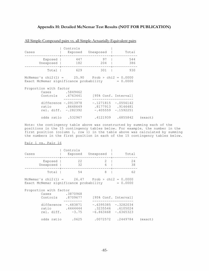
Appendix H: Detailed McNemar Test Results (NOT FOR PUBLICATION)

All Simple-Compound pairs vs. all Simple-Actuarially-Equivalent pairs

| Controls |Cases | Exposed Unexposed | Total-----------------+------------------------+------------ Exposed | 447 97 | 544 Unexposed | 182 204 | 386-----------------+------------------------+------------ Total | 629 301 | 930

McNemar's chi2(1) = 25.90 Prob > chi2 = 0.0000Exact McNemar significance probability = 0.0000

Proportion with factor Cases .5849462 Controls .6763441 [95% Conf. Interval] --------- -------------------- difference -.0913978 -.1271815 -.0556142 ratio .8648649 .8177913 .9146481 rel. diff. -.282392 -.405559 -.1592251

odds ratio .532967 .4121939 .6855842 (exact)

Note: the contingency table above was constructed by summing each of thepositions in the 15 contingency tables below. For example, the number in thefirst position (column 1, row 1) in the table above was calculated by summingthe numbers in the first position in each of the 15 contingency tables below.

Pair 1 vs. Pair 16

| Controls |Cases | Exposed Unexposed | Total-----------------+------------------------+------------ Exposed | 22 2 | 24 Unexposed | 32 6 | 38-----------------+------------------------+------------ Total | 54 8 | 62

McNemar's chi2(1) = 26.47 Prob > chi2 = 0.0000Exact McNemar significance probability = 0.0000

Proportion with factor Cases .3870968 Controls .8709677 [95% Conf. Interval] --------- -------------------- difference -.483871 -.6395385 -.3282034 ratio .4444444 .3235546 .6105024 rel. diff. -3.75 -6.863468 -.6365323

odds ratio .0625 .0072572 .2449784 (exact)

-85-

Pair 2 vs. Pair 17

| Controls |Cases | Exposed Unexposed | Total-----------------+------------------------+------------ Exposed | 58 1 | 59 Unexposed | 3 0 | 3-----------------+------------------------+------------ Total | 61 1 | 62

McNemar's chi2(1) = 1.00 Prob > chi2 = 0.3173Exact McNemar significance probability = 0.6250

Proportion with factor Cases .9516129 Controls .983871 [95% Conf. Interval] --------- -------------------- difference -.0322581 -.1110998 .0465837 ratio .9672131 .9060347 1.032522 rel. diff. -2 -8.789514 4.789514

odds ratio .3333333 .0063495 4.151441 (exact)

Pair 3 vs. Pair 18

| Controls |Cases | Exposed Unexposed | Total-----------------+------------------------+------------ Exposed | 38 1 | 39 Unexposed | 17 6 | 23-----------------+------------------------+------------ Total | 55 7 | 62

McNemar's chi2(1) = 14.22 Prob > chi2 = 0.0002Exact McNemar significance probability = 0.0001

Proportion with factor Cases .6290323 Controls .8870968 [95% Conf. Interval] --------- -------------------- difference -.2580645 -.3919297 -.1241993 ratio .7090909 .5925527 .8485489 rel. diff. -2.285714 -4.438998 -.1324308

odds ratio .0588235 .0014075 .3754091 (exact)

-86-

Pair 4 vs. Pair 19

| Controls |Cases | Exposed Unexposed | Total-----------------+------------------------+------------ Exposed | 7 6 | 13 Unexposed | 7 42 | 49-----------------+------------------------+------------ Total | 14 48 | 62

McNemar's chi2(1) = 0.08 Prob > chi2 = 0.7815Exact McNemar significance probability = 1.0000

Proportion with factor Cases .2096774 Controls .2258065 [95% Conf. Interval] --------- -------------------- difference -.016129 -.1461672 .1139091 ratio .9285714 .5499486 1.567864 rel. diff. -.0208333 -.169583 .1279163

odds ratio .8571429 .2379799 2.978588 (exact)

Pair 5 vs. Pair 20

| Controls |Cases | Exposed Unexposed | Total-----------------+------------------------+------------ Exposed | 12 6 | 18 Unexposed | 13 31 | 44-----------------+------------------------+------------ Total | 25 37 | 62

McNemar's chi2(1) = 2.58 Prob > chi2 = 0.1083Exact McNemar significance probability = 0.1671

Proportion with factor Cases .2903226 Controls .4032258 [95% Conf. Interval] --------- -------------------- difference -.1129032 -.2639309 .0381244 ratio .72 .4813126 1.077055 rel. diff. -.1891892 -.4409851 .0626067

odds ratio .4615385 .1438515 1.301504 (exact)

-87-

Pair 6 vs. Pair 21

| Controls |Cases | Exposed Unexposed | Total-----------------+------------------------+------------ Exposed | 35 6 | 41 Unexposed | 11 10 | 21-----------------+------------------------+------------ Total | 46 16 | 62

McNemar's chi2(1) = 1.47 Prob > chi2 = 0.2253Exact McNemar significance probability = 0.3323

Proportion with factor Cases .6612903 Controls .7419355 [95% Conf. Interval] --------- -------------------- difference -.0806452 -.2255601 .0642697 ratio .8913043 .7399666 1.073594 rel. diff. -.3125 -.8911317 .2661317

odds ratio .5454545 .1656336 1.609034 (exact)

Pair 7 vs. Pair 22

| Controls |Cases | Exposed Unexposed | Total-----------------+------------------------+------------ Exposed | 26 8 | 34 Unexposed | 16 12 | 28-----------------+------------------------+------------ Total | 42 20 | 62

McNemar's chi2(1) = 2.67 Prob > chi2 = 0.1025Exact McNemar significance probability = 0.1516

Proportion with factor Cases .5483871 Controls .6774194 [95% Conf. Interval] --------- -------------------- difference -.1290323 -.2966623 .0385978 ratio .8095238 .6278837 1.04371 rel. diff. -.4 -.9680515 .1680515

odds ratio .5 .1852586 1.238236 (exact)

-88-

Pair 8 vs. Pair 23

| Controls |Cases | Exposed Unexposed | Total-----------------+------------------------+------------ Exposed | 23 11 | 34 Unexposed | 11 17 | 28-----------------+------------------------+------------ Total | 34 28 | 62

McNemar's chi2(1) = 0.00 Prob > chi2 = 1.0000Exact McNemar significance probability = 1.0000

Proportion with factor Cases .5483871 Controls .5483871 [95% Conf. Interval] --------- -------------------- difference 0 -.164404 .164404 ratio 1 .7630866 1.310467 rel. diff. 0 -.3283231 .3283231

odds ratio 1 .3931661 2.543454 (exact)

Pair 9 vs. Pair 24

| Controls |Cases | Exposed Unexposed | Total-----------------+------------------------+------------ Exposed | 37 6 | 43 Unexposed | 9 10 | 19-----------------+------------------------+------------ Total | 46 16 | 62

McNemar's chi2(1) = 0.60 Prob > chi2 = 0.4386Exact McNemar significance probability = 0.6072

Proportion with factor Cases .6935484 Controls .7419355 [95% Conf. Interval] --------- -------------------- difference -.0483871 -.1863563 .0895821 ratio .9347826 .7881077 1.108755 rel. diff. -.1875 -.7045 .3295

odds ratio .6666667 .1952634 2.097224 (exact)

-89-

Pair 10 vs. Pair 25

| Controls |Cases | Exposed Unexposed | Total-----------------+------------------------+------------ Exposed | 45 3 | 48 Unexposed | 12 2 | 14-----------------+------------------------+------------ Total | 57 5 | 62

McNemar's chi2(1) = 5.40 Prob > chi2 = 0.0201Exact McNemar significance probability = 0.0352

Proportion with factor Cases .7741935 Controls .9193548 [95% Conf. Interval] --------- -------------------- difference -.1451613 -.2782711 -.0120515 ratio .8421053 .7283504 .9736266 rel. diff. -1.8 -4.340404 .7404037

odds ratio .25 .0452729 .9263782 (exact)

Pair 11 vs. Pair 26

| Controls |Cases | Exposed Unexposed | Total-----------------+------------------------+------------ Exposed | 27 11 | 38 Unexposed | 9 15 | 24-----------------+------------------------+------------ Total | 36 26 | 62

McNemar's chi2(1) = 0.20 Prob > chi2 = 0.6547Exact McNemar significance probability = 0.8238

Proportion with factor Cases .6129032 Controls .5806452 [95% Conf. Interval] --------- -------------------- difference .0322581 -.1250174 .1895335 ratio 1.055556 .832837 1.337834 rel. diff. .0769231 -.2469752 .4008214

odds ratio 1.222222 .460447 3.336929 (exact)

-90-

Pair 12 vs. Pair 27

| Controls |Cases | Exposed Unexposed | Total-----------------+------------------------+------------ Exposed | 26 14 | 40 Unexposed | 9 13 | 22-----------------+------------------------+------------ Total | 35 27 | 62

McNemar's chi2(1) = 1.09 Prob > chi2 = 0.2971Exact McNemar significance probability = 0.4049

Proportion with factor Cases .6451613 Controls .5645161 [95% Conf. Interval] --------- -------------------- difference .0806452 -.0857564 .2470467 ratio 1.142857 .888976 1.469244 rel. diff. .1851852 -.1290666 .4994369

odds ratio 1.555556 .6271247 4.074174 (exact)

Pair 13 vs. Pair 28

| Controls |Cases | Exposed Unexposed | Total-----------------+------------------------+------------ Exposed | 44 1 | 45 Unexposed | 10 7 | 17-----------------+------------------------+------------ Total | 54 8 | 62

McNemar's chi2(1) = 7.36 Prob > chi2 = 0.0067Exact McNemar significance probability = 0.0117

Proportion with factor Cases .7258065 Controls .8709677 [95% Conf. Interval] --------- -------------------- difference -.1451613 -.2597136 -.030609 ratio .8333333 .7303802 .9507986 rel. diff. -1.125 -2.309497 .0594969

odds ratio .1 .0023043 .702939 (exact)

-91-

Pair 14 vs. Pair 29

| Controls |Cases | Exposed Unexposed | Total-----------------+------------------------+------------ Exposed | 34 8 | 42 Unexposed | 12 8 | 20-----------------+------------------------+------------ Total | 46 16 | 62

McNemar's chi2(1) = 0.80 Prob > chi2 = 0.3711Exact McNemar significance probability = 0.5034

Proportion with factor Cases .6774194 Controls .7419355 [95% Conf. Interval] --------- -------------------- difference -.0645161 -.2211047 .0920725 ratio .9130435 .7479736 1.114542 rel. diff. -.25 -.8624887 .3624887

odds ratio .6666667 .2363844 1.773597 (exact)

Pair 15 vs. Pair 30

| Controls |Cases | Exposed Unexposed | Total-----------------+------------------------+------------ Exposed | 13 13 | 26 Unexposed | 11 25 | 36-----------------+------------------------+------------ Total | 24 38 | 62

McNemar's chi2(1) = 0.17 Prob > chi2 = 0.6831Exact McNemar significance probability = 0.8388

Proportion with factor Cases .4193548 Controls .3870968 [95% Conf. Interval] --------- -------------------- difference .0322581 -.1385308 .2030469 ratio 1.083333 .7376116 1.591096 rel. diff. .0526316 -.1933086 .2985718

odds ratio 1.181818 .4885561 2.913432 (exact)

-92-

Appendix I: Detailed Wald Test Results for Predictions (NOT FOR PUBLICATION)

1-in-1 Treatment: Wald tests for the null hypothesis of r = 0

Predicted r

p-value 0.45 0.48 0.49 0.53 0.59 0.62 0.64 0.67 0.75 0.78 0.80 0.83 0.89 0.93 0.94 0.97 # of Subjects

0 0 0 0 0 0 0 0 0 0 0 0 0 0 0 28 0 28

1.14E-34 0 0 0 0 0 0 0 0 0 0 0 0 0 0 0 16 16

1.33E-26 0 0 0 0 0 0 0 0 0 0 0 0 22 0 0 0 22

5.60E-25 0 0 0 0 0 0 0 9 0 0 0 0 0 0 0 0 9

6.78E-25 0 0 0 0 0 0 0 0 0 0 2 0 0 0 0 0 2

2.90E-22 0 0 0 0 0 0 17 0 0 0 0 0 0 0 0 0 17

2.02E-19 0 0 0 0 0 0 0 0 0 0 0 0 0 9 0 0 9

7.87E-19 0 0 0 0 0 0 0 0 0 0 0 2 0 0 0 0 2

1.12E-15 0 0 0 0 8 0 0 0 0 0 0 0 0 0 0 0 8

2.89E-13 0 0 0 0 0 5 0 0 0 0 0 0 0 0 0 0 5

3.05E-11 0 0 0 0 0 0 0 0 2 0 0 0 0 0 0 0 2

3.12E-09 0 0 0 0 0 0 0 0 0 3 0 0 0 0 0 0 3

4.42E-07 0 0 0 3 0 0 0 0 0 0 0 0 0 0 0 0 3

6.11E-07 0 0 2 0 0 0 0 0 0 0 0 0 0 0 0 0 2

0.0002934 4 0 0 0 0 0 0 0 0 0 0 0 0 0 0 0 4

0.0003798 0 1 0 0 0 0 0 0 0 0 0 0 0 0 0 0 1

# of Subjects 4 1 2 3 8 5 17 9 2 3 2 2 22 9 28 16 133

-93-

1-in-1 Treatment: Wald tests for the null hypothesis of gamma = 1

Predicted gamma

p-value 0.23 0.24 0.25 0.26 0.29 0.30 0.31 0.32 0.46 0.47 0.48 0.49 0.52 0.53 0.54 0.55 # of Subjects

7.02E-06 22 0 0 0 0 0 0 0 0 0 0 0 0 0 0 0 22

0.000047 0 0 0 0 0 0 0 0 0 17 0 0 0 0 0 0 17

0.0000525 0 28 0 0 0 0 0 0 0 0 0 0 0 0 0 0 28

0.0001667 0 0 0 0 0 0 0 0 8 0 0 0 0 0 0 0 8

0.0002153 0 0 0 0 2 0 0 0 0 0 0 0 0 0 0 0 2

0.0004045 0 0 0 0 0 0 0 0 0 0 0 9 0 0 0 0 9

0.000434 0 0 0 0 0 2 0 0 0 0 0 0 0 0 0 0 2

0.0004769 0 0 0 0 0 0 0 2 0 0 0 0 0 0 0 0 2

0.0005309 0 0 0 0 0 0 3 0 0 0 0 0 0 0 0 0 3

0.0007535 0 0 9 0 0 0 0 0 0 0 0 0 0 0 0 0 9

0.001047 0 0 0 16 0 0 0 0 0 0 0 0 0 0 0 0 16

0.0022308 0 0 0 0 0 0 0 0 0 0 5 0 0 0 0 0 5

0.0147585 0 0 0 0 0 0 0 0 0 0 0 0 0 0 0 3 3

0.0306056 0 0 0 0 0 0 0 0 0 0 0 0 0 0 1 0 1

0.0315525 0 0 0 0 0 0 0 0 0 0 0 0 0 2 0 0 2

0.0396612 0 0 0 0 0 0 0 0 0 0 0 0 4 0 0 0 4

# of Subjects 22 28 9 16 2 2 3 2 8 17 5 9 4 2 1 3 133

-94-

1-in-40 Treatment: Wald tests for the null hypothesis of r = 0

Predicted r

p-value 0.40 0.44 0.47 0.49 0.52 0.62 0.64 0.67 0.67 0.71 0.82 0.86 # of Subjects

1.96E-27 0 0 0 0 0 0 7 0 0 0 0 0 7

1.6E-24 0 0 0 0 0 0 0 0 0 0 8 0 8

1.56E-20 0 0 0 0 0 0 0 0 3 0 0 0 3

2.35E-18 0 0 0 0 0 0 0 0 0 11 0 0 11

1.25E-15 0 0 0 0 8 0 0 0 0 0 0 0 8

5.45E-14 0 0 0 0 0 0 0 4 0 0 0 0 4

3.92E-13 0 0 0 0 0 0 0 0 0 0 0 3 3

2.07E-10 0 0 0 11 0 0 0 0 0 0 0 0 11

8.76E-10 0 0 0 0 0 1 0 0 0 0 0 0 1

1.22E-08 0 0 3 0 0 0 0 0 0 0 0 0 3

0.000000917 0 1 0 0 0 0 0 0 0 0 0 0 1

0.0000284 2 0 0 0 0 0 0 0 0 0 0 0 2

# of Subject 2 1 3 11 8 1 7 4 3 11 8 3 62

-95-

1-in-40 Treatment: Wald tests for the null hypothesis of r + rc = 0

Predicted r + rc

p-value 0.54 0.57 0.59 0.63 0.66 0.67 0.71 0.73 0.74 0.76 0.81 0.84 # of Subjects

0.00E+00 0 0 0 0 0 0 0 3 0 0 0 0 3

9.27E-32 0 0 0 0 0 0 7 0 0 0 0 0 7

2.86E-25 0 0 0 0 0 0 0 0 4 0 0 0 4

3.55E-22 0 0 0 0 0 0 0 0 0 11 0 0 11

5.59E-19 0 0 0 0 0 0 0 0 0 0 0 3 3

7.64E-18 0 0 0 0 0 0 0 0 0 0 8 0 8

2.03E-17 0 0 0 11 0 0 0 0 0 0 0 0 11

7.91E-14 0 1 0 0 0 0 0 0 0 0 0 0 1

2.32E-12 0 0 0 0 0 1 0 0 0 0 0 0 1

1.5E-10 0 0 0 0 8 0 0 0 0 0 0 0 8

0.000000094 0 0 3 0 0 0 0 0 0 0 0 0 3

0.000000886 2 0 0 0 0 0 0 0 0 0 0 0 2

# of Subject 2 1 3 11 8 1 7 3 4 11 8 3 62

-96-

1-in-40 Treatment: Wald tests for the null hypothesis of γ = 1

Predicted gamma

p-value 0.37 0.41 0.68 0.75 0.79 0.95 0.99 1.06 1.26 1.30 1.33 1.37 # of Subjects

7.41E-03 0 8 0 0 0 0 0 0 0 0 0 0 8

0.0110372 3 0 0 0 0 0 0 0 0 0 0 0 3

0.0924481 0 0 0 0 0 0 0 0 0 0 0 11 11

0.1921943 0 0 0 0 0 0 0 0 0 0 8 0 8

0.1973165 0 0 0 11 0 0 0 0 0 0 0 0 11

0.2324818 0 0 1 0 0 0 0 0 0 0 0 0 1

0.2682751 0 0 0 0 0 0 0 0 0 2 0 0 2

0.3140454 0 0 0 0 0 0 0 0 1 0 0 0 1

0.3357557 0 0 0 0 3 0 0 0 0 0 0 0 3

0.8049443 0 0 0 0 0 0 0 3 0 0 0 0 3

0.8290983 0 0 0 0 0 4 0 0 0 0 0 0 4

0.9432108 0 0 0 0 0 0 7 0 0 0 0 0 7

# of Subjects 3 8 1 11 3 4 7 3 1 2 8 11 62

-97-

1-in-40 Treatment: Wald tests for the null hypothesis of γ + γc = 1

Predicted gamma + gammac

p-value 0.29 0.34 0.42 0.55 0.56 0.61 0.61 0.63 0.69 0.69 0.82 0.87 # of Subjects

4.02E-05 0 0 0 7 0 0 0 0 0 0 0 0 7

0.0001762 0 0 1 0 0 0 0 0 0 0 0 0 1

0.0002076 8 0 0 0 0 0 0 0 0 0 0 0 8

0.008463 0 3 0 0 0 0 0 0 0 0 0 0 3

0.0122949 0 0 0 0 3 0 0 0 0 0 0 0 3

0.0125595 0 0 0 0 0 0 11 0 0 0 0 0 11

0.0382169 0 0 0 0 0 4 0 0 0 0 0 0 4

0.062012 0 0 0 0 0 0 0 0 0 3 0 0 3

0.0686239 0 0 0 0 0 0 0 0 1 0 0 0 1

0.0960365 0 0 0 0 0 0 0 2 0 0 0 0 2

0.2874661 0 0 0 0 0 0 0 0 0 0 11 0 11

0.3762546 0 0 0 0 0 0 0 0 0 0 0 8 8

# of Subject 8 3 1 7 3 4 11 2 1 3 11 8 62

-98-