Reducing Trace Selection Footprint for Large-scaleJava Applications without Performance Loss

Peng Wu Hiroshige Hayashizaki Hiroshi Inoue Toshio Nakatani

IBM Research

pengwu@us.ibm.com,{hayashiz,inouehrs,nakatani}@jp.ibm.com

AbstractWhen optimizing large-scale applications, striking the bal-ance between steady-state performance, start-up time, andcode size has always been a grand challenge. While recentadvances in trace compilation have significantly improvedthe steady-state performance of trace JITs for large-scaleJava applications, the size control aspect of a trace compi-lation system remains largely overlooked. For instance, us-ing the DaCapo 9.12 benchmarks, we observe that 40% oftraces selected by a state-of-the-art trace selection algorithmare short-lived and, on average, each selected basic block isreplicated 13 times in the trace cache.

This paper studies the size control problem for a class ofcommonly used trace selection algorithms and proposes sixtechniques to reduce the footprint of trace selection withoutincurring any performance loss. The crux of our approach isto target redundancies in trace selection in the form of eithershort-lived traces or unnecessary trace duplication.

Using one of the best performing selection algorithmsas the baseline, we demonstrate that, on the DaCapo 9.12benchmarks and DayTrader 2.0 on WebSphere ApplicationServer 7.0, our techniques reduce the code size and com-pilation time by 69% and the start-up time by 43% whileretaining the steady-state performance. On DayTrader 2.0,an example of large-scale application, our techniques alsoimprove the steady-state performance by 10%.

Categories and Subject Descriptors D.3.4 [Processors]:Compilers, Optimization, Run-time environments

General Terms Algorithms, Experimentation, Performance

Keywords Trace selection and compilation, profiling, Java

Permission to make digital or hard copies of all or part of this work for personal orclassroom use is granted without fee provided that copies are not made or distributedfor profit or commercial advantage and that copies bear this notice and the full citationon the first page. To copy otherwise, to republish, to post on servers or to redistributeto lists, requires prior specific permission and/or a fee.

OOPSLA’11, October 22–27, 2011, Portland, Oregon, USA.Copyright c© 2011 ACM 978-1-4503-0940-0/11/10. . . $10.00

1. Introduction1.1 Trace compilation for large applications

How to effectively optimize large-scale applications has al-ways posed a great challenge to compilers. Although methodinlining expands the compilation scope of a method JIT,its effectiveness can be limited when the compilation targetlacks hot-spots and has numerous calling contexts and deepcall chains, all of which are common in large-scale Java ap-plications.

While trace-based compilation was traditionally exploredwhere mature JITs are absent, such as binary translators [1,6, 7], easy-to-develop JITs [10, 21], and scripting lan-guages [2, 4, 5, 8, 17], we explore trace compilation forJava, focusing on large-scale applications. To our problemdomain, the promise of trace-based compilation lies in itspotential to construct better compilation scopes than methodinlining does. In a trace compiler, a trace is a single-entrymultiple-exit region formed out of instructions following areal execution path. The most appealing trait of traces is itsability to span many layers of method boundaries, naturallyachieving the effect of partial inlining [20], especially indeep calling contexts.

The challenges of trace compilation for Java are alsoaplenty. As a first step, recent work in [13, 16] has signif-icantly bridged the performance gap between trace compi-lation and the state-of-the-art method compilation for Java,where a trace JIT is able to reach 96% of the steady-stateperformance of a mature product JIT on a suite of large-scaleapplications. This is achieved primarily by aggressively de-signing the trace selection algorithm to create larger traces.

1.2 Space Efficiency of Trace Selection

A trace selection design needs to optimize all aspects of sys-tem performance including steady-state performance, start-up and compilation time and binary code size. While opti-mizing for steady-state performance often leads to selectionalgorithms that maximize trace scope, such a design often in-creases start-up and compilation time, and binary code size.The latter three all relate to one trace selection metrics asdefined below.

Definition 1 Selection footprint is defined as the cumulativesize of all traces formed by a selection algorithm.

We use space efficiency to refer to a trace selection algo-rithm’s ability to maximize steady-state performance withminimal selection footprint. Space efficiency is especiallyimportant for large-scale applications where memory sub-system and compilation resources can be stressed. For ex-ample, code size bloat can degrade the steady-state perfor-mance due to bad instruction cache performance.

While space efficiency of trace selection was not ex-tensively studied before as most trace JITs target small ormedium size workloads, space considerations have been in-corporated into existing selection algorithms. The commonapproaches fall into the following categories:

• Selecting from hot regions. Several trace JITs [2, 8, 10]select traces only out of hot code regions, such as loops.This approach achieves superb space efficiency whendealing with codes with obvious hot spots, but not forlarge-scale applications, which often exhibit large, flatexecution profile.

• Limiting trace size. This approach limits individual tracesize using heuristics expressed as trace termination con-ditions, such as terminating trace recording at loop head-ers, at existing trace heads (known as stop-at-existing-head), or when exceeding buffer length. These heuris-tics, however, sometimes can significantly degrade theperformance. For instance, we observe up to 2.8 timesslower performance after applying the stop-at-existing-head heuristic. The space and performance impact of ex-isting trace termination heuristics are summarized in Sec-tion 6.

• Trace grouping. This approach groups linear traces sothat common paths across linear traces can be merged [2,8, 10, 14]. Existing trace grouping algorithms focussolely on loop regions. However, they have yet to demon-strate the ability to reach the required level of selectioncoverage for large-scale non loop-intensive workloads.

When dealing with large-scale applications, existing ap-proaches are either ineffective or insufficient in reducing se-lection footprint, or otherwise degrade steady-state perfor-mance. In this paper, we focus on improving the space ef-ficiency of trace selection by reducing selection footprintwithout degrading the steady-state performance for large-scale applications.

1.3 Key Observations

We focus on a class of commonly used trace selection al-gorithms, pioneered by Dynamo [1] and subsequently usedin [5, 12, 14, 17, 21] as well as the Java trace JIT mentionedearlier. In the paper, the specific selection algorithm used isderived from [16] and is referred to as the baseline algo-rithm throughout the paper.

0%

10%

20%

30%

40%

50%

60%

70%

80%

90%

100%

Day

Tra

der

avro

ra

batik

eclip

se fop h2

jyth

on

luin

dex

luse

arch

pmd

sunf

low

tom

cat

trad

ebea

ns

xala

n

geom

ean

Figure 1. Percentage of traces selected by the baseline algo-rithm with less than 500 execution count during steady-stateexecution.

While the baseline algorithm is one of the best perform-ing of its kind, it exhibits serious space efficiency issues. Fig-ure 2 shows the traces selected by the baseline algorithm fora simple example of 5 basic blocks. In total, the baseline al-gorithm creates four traces (A-D) with a selection footprintof 18 basic blocks and a duplication factor of 3.6.

We identify two sources of space inefficiency in the base-line algorithm that we will briefly describe below.

Formation of short-lived traces refers to a phenomenonwhere some traces are formed but seldom executed. Toquantify this effect, we measured the execution count oftraces formed by the baseline algorithm. Figure 1 showsthat 38% traces formed for the DaCapo 9.12 benchmarksand the DayTrader benchmark have less than 500 execu-tion counts during steady-state runs.1

Intuitively, a trace becomes dead when its entry pointis completely covered by traces formed later but whoseentry points are topologically earlier. At that point, theoriginal trace is no longer executed. This is analogous torendering a method “dead” after inlining the method toall its call-sites.

Non-profitable trace duplication refers to the duplicationof codes within or across traces that do not improveperformance. While previous work focuses primarily ontraces that are created unnecessarily long, we identifiedanother cause of the problem, that is, duplication dueto convergence of a selection algorithm. In this context,convergence refers to the state where a working set iscovered completely by existing traces so that no morenew traces are created.

1 For cyclic traces, execution counts include the number of times the tracecycles back to itself.

Figure 2. A working example: trace formation by the baseline algorithm.

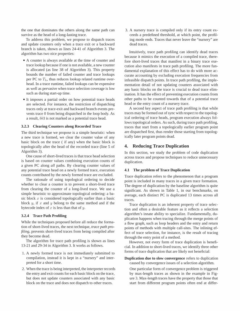
Figure 3. An example of low convergence due to form-ing max-length traces: when the trace buffer size (3BB) issmaller than loop body size (4BB), the algorithm takes 4traces to converge.

The problem stems from the fact that a trace can start andend at arbitrary program points, which in the presenceof tracing through cyclic paths could lead to pathologicalconvergence. Figure 3 gives such an example: when thecritical path of the loop body is too large to fit into asingle trace, many largely overlapping traces are formed,all of which start and end at slightly different programpoints.

1.4 Evaluation and Contribution

In this paper, we proposed six techniques to collectively ad-dress the problems of short-lived trace formation (in Sec-tion 3) and trace duplication (in Section 4).

We have implemented the proposed techniques in a Javatrace JIT based on IBM J9 JVM and JIT compiler. Thetechniques are applied to the baseline algorithm from [16],which has been heavily optimized for steady-state perfor-mance. After applying our techniques, we are able to re-duce the code size and compilation time by 69%, and thestart-up time by 43%, and with no degradation to the steady-state performance of the DaCapo 9.12 benchmarks and areal-world large-scale Java application, DayTrader on topof IBM’s Websphere application server. On DayTrader, ourtechniques improved the steady-state performance by 10%due to better cache performance.

The paper makes the following contributions:

• Deepen the understanding of the space efficiency prob-lem for a class of commonly used selection algorithmsand expanded the solution space.

• Identify the problem of short-lived trace formation andproposed techniques to reduce short-lived traces.

• Identify new sources of trace duplication problem andproposed trace truncation to reduce non-profitable dupli-cation.

• Demonstrate the effectiveness of our techniques on a setof large-scale Java applications.

2. The Baseline Trace Selection AlgorithmThe baseline algorithm is a one-pass selection algorithmderived from the one used in [16]. One-pass selection al-gorithms form traces that are either straight-line or cyclicand contain no inner join or split points. One-pass trace se-lection algorithms are the most common type of selectionalgorithms, which include NET [1], LEI [14], YETI [21],PyPy [5], and LuaJIT [17]. It has been demonstrated thatone-pass trace selection can scale to large applications andachieve the kind of coverage and performance comparableto those of a mature method JIT [13, 16].

A typical one-pass trace selection algorithm consists oftwo steps. First, it identifies a set of program points calledpotential trace head, and monitors their execution counts.Once the execution count of a potential trace head exceedsa threshold, trace recording is triggered, where it simplyrecords every instruction following the execution of the tracehead into a buffer called the recording buffer. Trace record-ing continues until a trace termination condition is satisfied,at which point, a new trace for the selected trace head isformed out of the recording buffer. The rest of the sectiondescribes these two components in detail.

The rest of the paper uses a working example to illustratevarious aspects of trace selection. Figure 2 shows a codefragment that sums the number of characters in an array ofstrings (countChar) and the traces formed by the baselineselection algorithm.

2.1 Trace Head Selection

The main driver of the baseline algorithm is shown in Al-gorithm 1. TraceSelection(e) is invoked every time the in-terpreter dispatches a control-flow event, which can be 1)control-flow bytecodes such as invoke, branch and return, or2) when an exit is taken from a trace.

The baseline algorithm identifies two types of potentialtrace heads (lines 17-19 in Algorithm 1). The first type isthe target of a backward branch, such as bb2 on trace A inFigure 2. This heuristic approximates loop headers withoutconstructing a control-flow graph. The second type is thetarget of a trace-exit (exit-head), such as bb4 on trace Bin Figure 2.2 This allows traces to be formed out of sidebranches of a trace.

The algorithm profiles the execution counts of potentialtrace heads such that those whose execution counts exceeda threshold, Th, trigger a new trace recording (lines 21-27in Algorithm 1). The algorithm assumes that counters andtraces are kept in a PC-indexed global map that is manip-ulated by getCounter and getTrace that return the counterand trace associated with a PC, respectively, and by getAd-

2 Prior to enter the loop in Figure 2, trace 0 is already formed from theentry point of String.length and includes codes following the returnof String.length from a different calling context. Therefore, When theexecution enters trace 0 from the loop, a trace exit is taken at the end of bb0.

Algorithm 1 TraceSelection(e), baselineInput: Let e be a control-flow event, PC be target PC of e,

and buf be the recording buffer1: /* trace recording and termination */2: if mode = record then3: if ShouldEndTrace(e) then4: mode← default5: create trace from buf then submit to compilation6: else7: append(buf ,e)8: end if9: return

10: end if11: /* trace dispatch */12: if getTrace(PC) �= null then13: dispatch to trace execution14: return15: end if16: /* identify potential trace head */17: if (isBackwardBranch(e) or isTraceExit(e)) then18: ctr ←getAddCounter(PC)19: end if20: /* trace head selection and start recording */21: if (ctr ← getCounter(PC)) �= null then22: ctr + +23: if ctr > Th then24: mode← record, buf ← ∅25: append(buf ,e)26: end if27: end if28: return

dCounter that, in addition, allocates a new counter if noneexists for a PC.

The rest of the algorithm covers trace dispatch (lines 12-15 in Algorithm 1) and trace recording (lines 2-10 in Algo-rithm 1), where its principle component, trace terminationconditions, are described in Section 2.2 and Algorithm 2.

2.2 Trace Termination conditions

Trace termination conditions are the primary mechanismin a selection algorithm to control the formation of a tracefor a given trace head.

Algorithm 2, ShouldEndTrace(e), describes the termina-tion conditions used in the baseline algorithm. This particu-lar choice of termination conditions is intended to maximizethe number of cyclic traces and the length of linear traces,both of which imply large scope for compilation and lesstrace transition overhead [13, 22]. Like any other selectionalgorithm, the baseline algorithm must address the follow-ing key aspects of when to end a trace recording.

Repetition detection ends the recording when a cyclic rep-etition path is detected in the recorded trace. Repetition

Algorithm 2 ShouldEndTrace(e), baselineInput: Let e be a control-flow event, PC be target PC of eOutput: true if the trace should be terminated at e, or false

if trace recording should continue.1: if PC is already recorded on the trace and not a false-

loop then2: if PC is not the trace head then3: set trace length be the index of the repeating PC4: end if5: return true6: else if recording buffer overflows then7: return true8: else if e is an JNI call that cannot be included on trace

then9: return true

10: else if e is an irregular event (e.g., exception) then11: return true12: else13: return false14: end if

detection is necessary for the convergence of the selec-tion algorithm as well as the formation of cyclic traces.

The baseline algorithm (lines 1-5 in Algorithm 2) detectsrepetition when current program counter (PC) is alreadyrecorded in the buffer (stop-at-repeating-pc) [14] andwhen the cycle is not a false loop [13].

When a repeating PC appears at the beginning of therecording buffer, such as traces A, B, and D in Figure 2,a cyclic trace is formed. Sometimes the repeating PCappears in the middle of the recording buffer (rejoined),then the recording buffer is backtracked to the rejoinedpoint to avoid introducing inner join to the trace, such astrace C in Figure 2.

Buffer overflow ends the recording when the recordingbuffer reaches its size limit (lines 6-7 in Algorithm 2).

Tracing out-of-scope ends the recording when an eventoutside the tracing scope has occurred, such as invok-ing a native call.

Tracing scope is a property of the trace system and maynot be violated as it may result in incorrect traces. In oursystem, tracing beyond an exception throw or a JNI callis not allowed (lines 8-11 in Algorithm 2).

2.3 Characteristics of the Baseline Algorithm

The baseline algorithm is designed to maximize the steady-state performance and reuses many existing heuristics inother systems.

Table 1 summarizes the basic characteristics of tracesselected by the baseline algorithm for the DaCapo 9.12 andthe DayTrader 2.0 benchmarks (setup details in Section 5).

Benchmark Description coverage # traces bbs/trace dup factor call/traceavrora simulates programs running on AVR microcontrollers 100.0% 1853 43 11 27batik produces SVG images based on unit tests in Apache Batik 99.7% 4817 43 11 26eclipse executes the jdt performance tests for Eclipse 99.9% 27862 40 15 21fop parse and format an XSL-FO file and generate a PDF file 99.7% 6096 62 19 41h2 a JDBCbench-like in-memory benchmark 100.0% 4124 57 17 34jython interprets the pybench Python benchmark 99.7% 10109 77 20 50luindex uses lucene to indexes a set of documents 99.9% 1376 31 7 17lusearch uses lucene to do a text search of keywords 100.0% 1447 39 9 23pmd analyzes Java classes for a set of source code problems 98.6% 7029 56 25 33sunflow renders a set of images using ray tracing 100.0% 1624 44 11 29tomcat query against Tomcat to retrieve/verify webpages 99.4% 17155 49 13 28tradebeans DayTrader via Java Beans on top of GERONIMO and h2 100.0% 8621 47 9 28xalan transforms XML documents into HTML 99.5% 3119 59 15 35DayTrader DayTrader 2.0 on IBM WebSphere Application Server 7.0 100% 19809 69 15 40

geomean 99.7% 3869 49 13 30

Table 1. Characteristics of traces formed by the baseline algorithm for DaCapo 9.12 and Daytrader benchmarks. Coverage isthe percentage of total bytecodes executed from traces; # traces is the number of compiled traces; bbs/trace is average numberof basic blocks per trace; dup factor is the ratio between the number of bytecodes on traces and that of bytecodes in distinctbasic blocks on traces; and call/trace is the number of invoke or return bytecodes per trace.

One important characteristic is the coverage of a trace se-lection. High coverage is a particular requirement for a byte-code trace JIT like ours where more than ten-fold perfor-mance gap exists between being “covered” (compiled) and“not covered” (interpreted) by the trace JIT. As shown in Ta-ble 1, the algorithm achieves close to 100% coverage at thesteady-state, similar to that of the method JIT.

Table 1 also shows other static characteristics of the traceselection. The number of traces selected ranges from 1400to 27K, indicating the algorithm’s ability to support largeworking sets. It is also observed that traces formed by thebaseline algorithm are quite long with an average 49 basicblocks per trace and can span many layers of method bound-aries, where, on average, 30 invoke or return bytecodes areincluded per trace.

3. Reducing Short-lived TracesIn this section, we propose a set of techniques that reduce

selection footprint without degrading the performance bytargeting traces that are short lived.

3.1 Short-lived Trace Formation

Short-lived trace formation refers to the phenomenon thatthe selection algorithm creates traces that become dead shortafter their creation. For instance, the baseline algorithm firstcreates trace B in Figure 2, and shortly after trace A iscreated.3 Since the head of trace B (bb3) is dominated bythat of trace A (bb1) and is included in trace A, the creationof trace A renders trace B dead.

3 Trace B is created before A because the baseline algorithm identifies bb3as a potential trace head first, before the first backward branch targeting bb1is taken.

Intuitively, a trace becomes dead when the head of thetrace is completely covered by later formed traces such thatthe trace is no longer dispatched. A formal definition of deadtraces is given below.

Definition 2 An instruction x is an infeasible dispatch pointat time t, if after t, there is no invocation of TraceSelection(e)where the target of e is x.

Definition 3 A trace A starting from x becomes dead at timet if, after t, x becomes an infeasible dispatch point.

Short-lived trace formation is an inherent property ofa trace selection algorithm that satisfies the following twoconditions.

Condition 1 Two traces may be dispatched in the reverseorder of how their corresponding trace heads are selected.

Condition 2 The head of an earlier trace can be part of alater trace.

The baseline algorithm satisfies both conditions. Condi-tion 1 is a property of trace head selection. Most selection al-gorithms satisfies this condition because there is no guaran-teed ordering on how a trace head is selected. Potential traceheads may accumulate counter values at different speed. Forinstance, basic blocks at control-flow join are executed moreoften than their predecessors.

Condition 2, on the other hand, is a property of tracetermination conditions. Certain termination conditions, suchas stop-at-existing-head, can prevent the condition to besatisfied.

Algorithm 3 TraceSelectionWithSizeControl(e), optimizedInput: Let e be a control-flow or an exact-bb event, PC be

target PC of e, Ph and Th be the profiling and trace-headthreshold, and buf be the recording buffer.

1: /* trace recording */2: if mode = record then3: if ShouldEndTrace(e) then4: StructureTruncation(buf, e)5: clear counters (if any) of bbs in buf6: create trace from buf , mode← default7: else8: append(buf ,e)9: end if

10: return11: end if12: /* trace path profiling */13: if curr tr �= null then14: if PC = getStartPC(curr tr, curr pos) then15: curr pos + +16: return17: else18: incExitFreq(curr tr,curr pos)19: curr tr ← null20: end if21: end if22: /* trace head selection and dispatch */23: if isBackwardBranch(e) or isTraceExit(e) then24: if (tr ← getTrace(PC)) �=null then25: if isCompiled(tr) then26: dispatch to binary address of tr27: else28: /* enter trace path profiling mode */29: tr.entryFreq++30: if tr.entryFreq > Ph then31: profileTruncation(tr)32: submit tr to compilation queue33: end if34: curr pos + +, curr tr ← tr35: end if36: return37: end if38: ctr ← getAddCounter(PC)39: if (+ + ctr) > Th then40: mode← record, buf ← ∅, append(buf , e)41: end if42: end if43: return

3.2 Short-lived Trace Elimination

In this section, we identify the causes of short-lived trace for-mation in the baseline algorithm and propose a more spaceefficient algorithm, TraceSelectionWithSizeControl(e), asshown in Algorithm 3.

The new algorithm creates only 2 traces for the workingexample, trace A and a trace that contains bytecode 0-4,with a selection footprint of 5 basic blocks and a duplicationfactor of 1. This is in contrast to the selection footprint of 18basic blocks by the baseline algorithm as shown in Figure 2.The rest of the section describes the new algorithm in detail.

3.2.1 Constructing Precise Basic Blocks

In the baseline algorithm, TraceSelection(e) is invoked everytime the interpreter executes a control-flow bytecode. Thebytecode sequence between consecutive control-flow byte-codes is called a dynamic instruction block. Dynamic in-struction blocks can be partially overlapping, such as bb1+2and bb2 of trace C in Figure 2. We refer to such dynamic in-struction blocks as imprecise basic blocks.

Dynamic instruction blocks can trigger the formation ofshort-lived traces. Consider the formation of trace C and Din Figure 2. A trace recording starts from bytecode 0 andcontinues through two iterations of the loop. The recordingis terminated when a repeating PC, bytecode 10, is detectedin the middle of the recording buffer. Trace C is formedby backtracking the recorded trace to bytecode 10, and thentrace D is created from the target of the end-exit from traceC. Once trace C and D are formed, trace A and B becomedead because their respective entry points, bb2 and bb4 be-come infeasible dispatch points.

Such short-lived traces are caused by the terminationcondition that detects repetition by checking repeating PCs(as line 1 of Algorithm 2) at control-flow bytecodes. Thistermination condition works fine only when two distinctbasic blocks are disjoint. Because of imprecise basic blocks,the baseline algorithm detects bytecode 10 as the repeatingPC in the recording buffer, whereas bytecode 4 is the actualfirst repeating PC.

To address this problem, we identify boundaries of pre-cise basic blocks and call TraceSelection(e) at the end ofeach precise basic block. The new algorithm correctly de-tects that bytecode 4 is the first repeating PC in the recordingbuffer.

3.2.2 Trace-head Selection Optimization

The baseline algorithm performs two lookups for each in-vocation of TraceSelection(e): 1) look up and dispatch thetrace for event e (lines 12-15 of Algorithm 1), and 2) lookup and update the counter associated with e (lines 21-27 ofAlgorithm 1). While this design dispatches traces and ac-cumulate frequency counts as fast as possible, it can causepathological formation of short-lived traces.

Consider the formation of trace A and B. Despite theloop body having only a single execution path, the baselinealgorithm identified two potential trace heads, bb1 (the targetof a backward branch) and bb3 (the target of a side-exit fromtrace 0). Selecting multiple potential trace heads along onecritical path can result in short-lived traces because only

the one that dominates the others along the same path cansurvive as the head of a long-lasting trace.

To address this problem, we propose to dispatch tracesand update counters only when a trace exit or a backwardbranch is taken, shown as lines 24-41 of Algorithm 3. Thealgorithm has two nice properties:

• A counter is always available at the time of counter andtrace lookup because if one is not available, a new counteris allocated (as line 38 of Algorithm 3). This propertybounds the number of failed counter and trace lookupsper PC to Th, thus reduces lookup related runtime over-head. In a trace runtime, failed lookups can be expensiveas well as pervasive when trace selection coverage is lowsuch as during start-up time.

• It imposes a partial order on how potential trace headsare selected. For instance, the restriction of dispatchingtraces only at trace-exit and backward branch events pre-vents trace 0 from being dispatched in the loop body. Asa result, bb3 is not marked as a potential trace head.

3.2.3 Clearing Counters along Recorded Trace

The third technique we propose is a simple heuristic: whena new trace is formed, we clear the counter value of anybasic block on the trace ( if any) when the basic block istopologically after the head of the recorded trace (line 5 ofAlgorithm 3).

One cause of short-lived traces is that trace head selectionis based on counter values combining execution counts ofa given PC along all paths. By clearing counter values ofany potential trace head on a newly formed trace, executioncounts contributed by the newly formed trace are excluded.

The rationale of using topological ordering to decidewhether to clear a counter is to prevent a short-lived tracefrom clearing the counter of a long-lived trace. We use asimple heuristic to approximate topological ordering: a ba-sic block x is considered topologically earlier than a basicblock y, if x and y belong to the same method and if thebytecode index of x is less than that of y.

3.2.4 Trace Path Profiling

While the techniques proposed before all reduce the forma-tion of short-lived traces, the next technique, trace path pro-filing, prevents short-lived traces from being compiled afterthey become dead.

The algorithm for trace path profiling is shown as lines13-21 and 29-34 in Algorithm 3. It works as follows.

1. A newly formed trace is not immediately submitted tocompilation, instead it is kept in a “nursery” and inter-preted for a short time.

2. When the trace is being interpreted, the interpreter recordsthe entry and exit counts for each basic block on the trace,but does not update counters associated with any basicblock on the trace and does not dispatch to other traces.

3. A nursery trace is compiled only if its entry count ex-ceeds a predefined threshold, at which point, the profil-ing mode ends. Traces that never leave the “nursery” aredead traces.

Intuitively, trace path profiling can identify dead tracesbecause it mimics the execution of a compiled trace, there-fore short-lived traces that manifest in a binary trace exe-cution also manifests in trace path profiling. The more fun-damental explanation of this effect has to do with more ac-curate accounting by excluding execution frequencies frominfeasible dispatch points. In trace path profiling, the imple-mentation detail of not updating counters associated withany basic blocks on the trace is crucial to dead trace elim-ination. It has the effect of preventing execution counts fromother paths to be counted towards that of a potential tracehead or the entry count of a nursery trace.

A second key aspect of trace path profiling is that whiletraces may be formed out of sync with respect to the topolog-ical ordering of trace heads, program execution always fol-lows topological orders. As such, during trace path profiling,traces that start from a topologically earlier program pointare dispatched first, thus render those starting from topolog-ically later program points dead.

4. Reducing Trace DuplicationIn this section, we study the problem of code duplicationacross traces and propose techniques to reduce unnecessaryduplication.

4.1 The problem of Trace Duplication

Trace duplication refers to the phenomenon that a programpoint is included in many traces in a given trace formation.The degree of duplication by the baseline algorithm is quitesignificant. As shown in Table 1, in our benchmarks, onaverage, each distinct PC is duplicated 13 times across alltraces.

Trace duplication is an inherent property of trace selec-tion and often a desirable feature as it reflects a selectionalgorithm’s innate ability to specialize. Fundamentally, du-plication happens when tracing through the merge points ofa flow graph, such as loop headers and the entry and returnpoints of methods with multiple call-sites. The inlining ef-fect of trace selection, for instance, is the result of tracingthrough the entry point of a method.

However, not every form of trace duplication is benefi-cial. In addition to short-lived traces, we identify three otherforms of trace duplication that are likely not beneficial:

Duplication due to slow convergence refers to duplicationcaused by convergence issues of a selection algorithm.

One particular form of convergence problem is triggeredby max-length traces as shown in the example in Fig-ure 3. Max-length traces have the property that those thatstart from different program points often end at differ-

Algorithm 4 StructureTruncation(buf ,bb)Input: Let buf be the trace recording buffer with n bbs,

ML be the maximal trace length, and bb be the bbexecuted after buf [n− 1]

Output: returns the length of the truncated trace.1: if buf is cyclic or n = 1 then2: return n3: end if4: for i← 1 to n− 1 do5: if isLoopHeader(buf [i]) then6: let L be the loop whose header is buf [i]7: if isloopExited(L, i, buf) = false then8: if trunc-at-entry-edge and isEntryEdge(buf [i−

1],buf [i]) then9: return i

10: end if11: if trunc-at-backedge and isBackEdge(buf [i −

1],buf [i]) then12: return i13: end if14: if trunc-at-loop-header then15: return i16: end if17: end if18: end if19: end for20: if n = MLandisTraceHead(bb) = false then21: for i← n− 1 to 1 do22: if isTraceHead(buf [i]) then23: Let tr be the trace whose head is buf [i]24: if match(buf [i : n),tr[0:n − i]) and isMethod-

Returned(i, buf )=false then25: return i26: end if27: end if28: end for29: end if30: return n

ent program points. When combined with tracing alongcyclic paths, this property can cause slow convergence ofa selection algorithm.

Loop-related duplication refers to duplication as the resultof tracing through a common type of control-flow join,loop headers.

One form of unnecessary duplication happens when trac-ing through the entry-edge of a loop. This is analogous toalways peeling the first iteration of a loop into a trace.

Another form of duplication happens when tracing throughthe backedge or exit-edge of a loop (also known as tailduplication).

Trace segment with low utilization refers to the case wherethe execution often takes a side-exit before reaching thetail segment of a trace.

The most common scenario of this problem manifestswhen a mega-morphic control-flow bytecode, such as thereturn bytecode from a method with many calling con-texts, appears in the middle of the trace. For example,trace A in Figure 2 contains a return bytecode fromString.length that has many different calling con-texts. As a result, the return bytecode on trace A is a hotside-exit and a good candidate for truncation.

4.2 Trace Truncation

We propose trace truncation that uses structure or profilinginformation to determine the most profitable end point ofa trace. We propose two types of trace truncation. One isstructure-based that applies truncation based on static prop-erties of a recorded trace (shown as StructureTruncation inAlgorithm 4). The other is profile-based that truncates basedon trace path profiling information (lines 31 in Algorithm 3).

Traditionally, a selection algorithm controls duplicationby imposing additional termination conditions. Comparedto this approach, trace truncation has the advantage of beingable to look ahead and use the knowledge on the path beyondto decide the most profitable trace end-point.

Since trace truncation may shorten lengths of activetraces, care must be taken to minimize degradation to per-formance. For this consideration, we define the followingguidelines of where not to apply truncation:

• Do not truncate cyclic traces. Cyclic traces can capturelarge scopes of computation that are disproportional to itssize, therefore the performance cost of a bad truncationmay outweigh the benefit of size reduction.

• Do not truncate between a matching pair of method entryand return. The rule preserves the amount of partial in-lining in a trace, which is a key indicator of trace qualityin our system.

• Do not truncate at non trace-heads. This rule preventstruncation from introducing new potential trace heads(thus new traces) and worsening the convergence of traceselection.

4.2.1 Structure-based Truncation

Structure-based truncation is applied immediately after atrace recording and ends before the trace is created. We pro-pose the following heuristics for structure-based truncation.The first three exploit loop structures for truncation. The lastone is specifically designed for max-length traces with noloop-based edges.

• trunc-at-loop-entry-edge that truncates at the entry-edgeto the first loop on the trace with more than one iteration.

This is based on the consideration that peeling the firstiteration of a loop is likely not profitable.

• trunc-at-loop-backedge that truncates at the backedge tothe first or last loop on the trace with more than oneiteration.

This is based on the consideration that the backedge isa critical edge that forms cycles. Therefore, truncation atbackedge may improve the convergence of the algorithm.This heuristic allows cyclic traces to be formed on loopheaders, but not on other program points in the loop.

• trunc-at-loop-header that truncates at the header of thefirst/last loop on the trace with more than one iteration.

This is a combination of the previous two heuristics.

• trunc-at-last-trace-head that truncates at the last locationon the trace, where 1) it is the head of an existing trace,2) the existing trace matches the portion of the trace tobe truncated, 3) it is not in between a matching pair ofmethod enter and return.

The structure-based truncation algorithm is given in Al-gorithm 4, where isMethodReturned checks whether a po-tential truncation point is between the entry and return ofa method on the trace; isLoopExited(L,i,buf ) assumes thatthe ith basic block in buf is the header of loop L and checksif the remaining portion of the trace exits from the body ofL4, and isEntryEdge (isBackEdge) checks whether an edgeis the loop entry-edge (backedge).

4.2.2 Profile-based Truncation

Profile-based truncation uses the profiling information col-lected by trace path profiling to truncate traces at hot side-exits (as line 31 in Algorithm 3).

For a given trace, trace path profiling collects the entrycount to a trace as well as trace exit count of each basic blockon the trace, i.e., the number of times execution leaves a tracevia this basic block. From trace exit counts, one can computethe execution count of each basic block on the trace. Profile-based trace truncation uses a simple heuristic: for a givenbasic block x on a trace, if the entry count of x on the traceis smaller than a predefined fraction of the entry count of thetrace, we truncate the trace at x. In our implementation, weuse a truncation threshold of 5%.

5. Evaluation5.1 Our Trace JIT System Overview

Figure 4 shows a component view of our trace JIT, which isbuilt on top of IBM J9 JVM and JIT compiler [11]. Tracesare formed out of Java bytecodes and compiled by the J9 JIT,which is extended to compile traces. Our trace JIT supportsboth trace execution and interpretation, as well as all majorfunctionality of the method JIT. Compilation is done by adedicated thread, similar to the method JIT.

4 In our implementation, we check if the remaining portion of the traceincludes codes from the same method but outside the loop body or whetherthe owning method of the loop header has returned. Both indicate that loopL has been exited.

Tracing runtime

interpreterinterpreter

trace (Java bytecode)

trace selectionengine

trace selectionengine

IR generatorIR generator optimizersoptimizers

code generatorcode generator

trace dispatchertrace dispatcher garbage collector

code cachecode cache

class libraries

trace cache(hash map)trace cache(hash map)

(e.g. hotness counter andcompiled code address)

Java VM

JIT compiler

modified componentmodified component

unmodified component

new componentnew component

execution events

compiled code

early redundancyelimination

early redundancyelimination

Figure 4. Overview of our trace JIT architecture

Trace head threshold 500 (BB exec freq)Trace buffer length 128 (BBs)Structure trunc. (rejoined) 1st loop-headerStructure trunc. (max-length) 1st loop-header or last trace-headTrace profiling window 128 (trace entry freq)Profile trunc. threshold 5%

Table 2. Trace selection algorithm parameters.

The trace compiler enables a subset of “warm” level opti-mizations of the baseline method JIT such as various (par-tial) redundancy elimination optimizations, (global) regis-ter allocation, and value propagation. Our system is aggres-sively optimized to reduce runtime overhead due to trace ex-ecution and trace monitoring (including trace linking opti-mizations). The current implementation also has limitationscompared to the method JIT. For example, the trace JIT doesnot support recompilation. It does not support escape anal-ysis and enables only a subset of loop optimizers in the J9JIT. Detailed design of the trace JIT is described in [16].

Table 2 summarizes some of the key parameters of theselection algorithm for the evaluation.

5.2 Experiment Setup

Experiments are conducted on a 4-core, 4GHz POWER6processors with 2 SMT threads per core. The system has 16GB of system memory and runs AIX 6.1. For the JVM, weuse 1 GB for Java heap size with 16MB large pages and thegenerational garbage collector. We used two benchmarks:

DaCapo 9.12 benchmark [3] running with the default datasize. We did not include the tradesoap benchmarkbecause the baseline system with the method-JIT some-times failed for this benchmark.

DayTrader 2.0 [19] running on IBM WebSphere Applica-tion Server version 7.0.0.13 [15]. This is an example oflarge-scale Java applications. For DayTrader, the DB2database server and the client emulator ran on separatemachines.

In this paper, we use the following metrics to evaluate ourtechniques. For each result, we report the average of 16 runsalong with the 95% confidence interval.

Selection footprint: the total number of bytecodes in com-piled traces.

Compiled binary code size: the total binary code size.

Steady-state execution time: For DaCapo 9.12, we exe-cuted 10 iterations for eclipse and 25 iterations forthe other benchmarks, and reported the average execu-tion time of the last 5 iterations. For DayTrader, we ranthe application for 420 seconds that includes 180-secondclient ramp-up but excludes setup and initialization, andused the average execution time per request during thelast 60 seconds.

Start-up time: the execution time of the first iteration forDaCapo 9.12, and the time spent before the WebSphereApplication Server becomes ready to serve for Day-Trader.

Compilation time: the total compilation time.

5.3 Reduction in Selection Footprint

We evaluated the six techniques proposed in this paper assummarized in Table 3. First, we measured the impact ofeach individual technique on selection footprint. Figure 5shows the normalized selection footprint when we applyeach technique to the baseline.

We observe that each technique is effective in reducingselection footprint, with the average reduction ranging from12% (exact-bb) to 40% (head-opt). The only exception iswhen applying head-opt to jython, where selection foot-print increases by 2%.

Second, we measured the combined effects of the tech-niques in reducing selection footprint, as shown in Figure 6.In this and following figures, the techniques are combinedaccording to the natural order (left to right) by which they areapplied during the selection. For example, the bar +struct-trunc stands for the case where we apply exact-bb, head-opt,and struct-trunc to the baseline.

With all techniques applied, the average selection foot-print is reduced to 30% of the baseline’s. We also observethat each technique is able to further reduce selection foot-print over the ones applied before it.

Figure 8 shows a detailed breakdown on where the reduc-tion in selection footprint comes from.

• The bottom bar our algo w/ all-opt is the selection foot-print of our algorithm relative to the baseline’s.

• Short-lived traces eliminated represent the total bytecodesize of short-lived traces eliminated by our optimizations.

• Structure truncated BCs and profile truncated BCs ac-count for bytecodes eliminated by structure-based andprofile-based truncation, respectively.

0%

10%

20%

30%

40%

50%

60%

70%

80%

90%

100%

Day

Tra

der

avro

ra

batik

eclip

se fop h2

jyth

on

luin

dex

luse

arch

pmd

sunf

low

tom

cat

trad

ebea

ns

xala

n

geom

ean

otherseliminated

profile-truncBCs

structure-truncBCs

short-livedtraceseliminatedour algo w/ all-opts

Figure 8. Breakdown of selection footprint reduction nor-malized to that of the baseline.

• Others represent the rest of the reduction, which is likelydue to improved convergence of the baseline algorithmthat generates fewer new traces.

5.4 Impact on System Performance

Figure 7 shows the combined impact of our techniques oncompiled binary code size. With all our techniques com-bined, the compiled code size is reduced to 30% of the base-line’s, which is consistent with the degree of reduction onselection footprint.

Figure 9 shows the combined impact of our techniques onsteady-state execution time. The steady-state performancewas unchanged on average after all techniques are applied,with a maximal degradation of 4% for luindex.

It is also notable that the steady-state performance ofDayTrader is improved by 10%. This is because L2 cachemisses were reduced and thus clock per instruction wasimproved, due to reduced code size. This shows that codesize control is not only important for memory reduction itselfbut also important for the steady-state performance in large-scale applications.

Figure 10 and Figure 11 show the normalized start-uptime and compilation time when the techniques are appliedin combination, respectively. Using our techniques, compi-lation time and start-up time was reduced to 32% and 57%of the baseline’s, respectively.

5.5 Discussions

Our results show that the reduction in selection footprintis linear to that of compilation time and binary code size.Start-up time is closely related to but not linear to selec-tion footprint because it is influenced by other factors suchas the ratio of interpretation overhead to native executionand how fast bytecodes are captured as traces and com-piled to binaries. Only very large-scale applications, such asDayTrader and eclipse, experience an improvement in

Name Description Described in Main effectexact-bb exact basic block construction Section 3.2.1 Reduced short-lived traces & duplicationhead-opt counter/trace lookup at backward branch and exit-heads Section 3.2.2 Reduced short-lived tracesstruct-trunc structure-based truncation Section 4.2.1 Reduced short-lived traces & duplicationclear-counter clearing counters of potential trace heads on a recorded trace Section 3.2.3 Reduced short-lived tracesprofile trace profiling Section 3.2.4 Reduced short-lived tracesprof-trunc trace profiling with profile-based truncation Section 4.2.2 Reduced duplication

Table 3. Summary of evaluated techniques

Day

Trad

er

avro

ra

batik

eclip

se fop h2

jyth

on

luin

dex

luse

arch

pmd

sunf

low

tom

cat

trad

ebea

ns

xala

n

geom

ean

baseline exact−bb head−opt clear−counter struct−trunc prof prof w/ trunc

Nor

mal

ized

Sel

ectio

n F

ootp

rint

0.0

0.5

1.0

1.5

2.0

Figure 5. Selection footprint (normalized to the baseline) when applying each technique (shorter is better).

Day

Trad

er

avro

ra

batik

eclip

se fop h2

jyth

on

luin

dex

luse

arch

pmd

sunf

low

tom

cat

trad

ebea

ns

xala

n

geom

ean

baseline +exact−bb +head−opt +clear−counter +struct−trunc +prof +prof w/ trunc

Nor

mal

ized

Sel

ectio

n F

ootp

rint

0.0

0.5

1.0

1.5

2.0

Figure 6. Selection footprint (normalized to the baseline) after combining techniques over the baseline (shorter is better).

Day

Trad

er

avro

ra

batik

eclip

se fop h2

jyth

on

luin

dex

luse

arch

pmd

sunf

low

tom

cat

trad

ebea

ns

xala

n

geom

ean

baseline +exact−bb +head−opt +clear−counter +struct−trunc +prof +prof w/ trunc methodJIT

Nor

mal

ized

Gen

erat

ed B

inar

y C

ode

Siz

e

0.0

0.5

1.0

1.5

2.0

Figure 7. Binary code size (normalized to the baseline) after combining techniques over the baseline (shorter is better).

Day

Trad

er

avro

ra

batik

eclip

se fop h2

jyth

on

luin

dex

luse

arch

pmd

sunf

low

tom

cat

trad

ebea

ns

xala

n

geom

ean

baseline +exact−bb +head−opt +clear−counter +struct−trunc +prof +prof w/ trunc methodJIT

Nor

mal

ized

Ste

ady−

stat

e E

xecu

tion

Tim

e

0.0

0.5

1.0

1.5

2.0

Figure 9. Steady-state execution time (normalized to the baseline) after combining techniques over the baseline (shorter isbetter).

steady-state performance as the result of selection footprintreduction.

Eliminating short-lived traces have the biggest impactin footprint reduction. Of all the techniques that eliminateshort-lived traces, ensuring proper ordering by which to se-lect trace heads (head-opt) addresses the root cause of shortlived traces.

We would also like to point out that some of the pro-posed techniques may potentially degrade start-up perfor-mance because they either reduce the scope of individualtraces (e.g., truncation) or prolongs the time before a byte-code is executed from a binary trace (e.g., profiling). Butour results show empirically that footprint reduction in gen-eral improves start-up performance because, for large-scaleworkloads, compilation speed is likely a more critical bot-

tleneck to the start-up time than other factors. However, thecost-benefit effects may change depending on the compila-tion resource of the trace compiler, the coverage require-ment of the selection algorithm, and the characteristics ofthe workload.

6. Comparing with Other SelectionAlgorithms

While our techniques are described in the context of thebaseline algorithm, many design choices are also commonin other trace selection algorithms. Table 4 summarizes im-portant aspects of trace selection discussed in the paper forall existing trace selection algorithms.

Day

Trad

er

avro

ra

batik

eclip

se fop h2

jyth

on

luin

dex

luse

arch

pmd

sunf

low

tom

cat

trad

ebea

ns

xala

n

geom

ean

baseline +exact−bb +head−opt +clear−counter +struct−trunc +prof +prof w/ trunc methodJIT

Nor

mal

ized

Sta

rt−

up T

ime

0.0

0.5

1.0

1.5

2.0

Figure 10. Start-up time (normalized to the baseline) after combining techniques over the baseline (shorter is better).

Day

Trad

er

avro

ra

batik

eclip

se fop h2

jyth

on

luin

dex

luse

arch

pmd

sunf

low

tom

cat

trad

ebea

ns

xala

n

geom

ean

baseline +exact−bb +head−opt +clear−counter +struct−trunc +prof +prof w/ trunc methodJIT

Nor

mal

ized

Com

pila

tion

time

0.0

0.5

1.0

1.5

2.0

2.5

3.0

Figure 11. Compilation time (normalized to the baseline) after combining techniques over the baseline (shorter is better).

6.1 One-pass selection algorithms

We first compare our techniques with size control heuristicsused in existing one-pass selection algorithms, all of whichare based on termination conditions.

Stop-at-existing-head terminates a trace recording whenthe next instruction to be recorded is the head of an exist-ing trace. This heuristic was first introduced by NET [1].It is most effective size-control heuristic because it min-imizes duplication across traces. It does not generateshort-lived traces either because Condition 2 of short-lived trace formation is no longer satisfied. However,stop-at-existing-head can have significant impact of per-formance due to reduced trace scope.

Figure 12 shows the relative execution time and codesize of stop-at-existing-head normalized to that of our

algorithm. It shows that stop-at-existing-head excels atspace efficiency, but degrades the performance by up to2.8 times.

A main source of the degradation comes from the re-duction in the inlining effect of the trace selection. Inparticular, once a trace is formed at the entry point of amethod, stop-at-existing-head prevents the method to be“inlined” into any later traces that invoke the method.

Stop-at-loop-boundary terminates a trace recording at loopboundaries, such as loop headers or loop exit-edges. Vari-ations of this heuristic are used in PyPy, TraceMonkey,HotpathVM, SPUR, and YETI.

We compared stop-at-loop-head heuristic, which is onetype of stop-at-loop-boundary and terminates a trace atloop headers (figure not included in the paper). On the

System our baseline SPUR HotpathVM LuaJIT TraceMonkey PyPy YETI NET Merrill+ LEI[13, 16] [2] [10] and [9] [17] [8] [5] [21] [1] [18] [14]

Target Program Java CIL Java Lua JavaScript Python Java Binary Java Binary

Multi-pass or one-pass selection one multi multi N/A multi one one one one one

Trace loop head Y Y Y Y Y Y Y Y Y Y

Head exit head Y Y Y Y Y N/A Y Y Y Y

Condition method entry Y Y

Trace stop-at-any-backward-branch Y YTermination stop-at-repeating-pc Y Y Y YCondition Stop-at-loop-back-to-head Y Y Y Y

stop-at-existing-trace-heads Y N/A call N/A Y Y Y

stop-when-leaving-static-scope loop method loop loop N/A N/A method

stop-when-exceeding-max-size Y Y Y Y Y Y Y Y Y Y

stop-at-native-method-call Y N/A N/A N/A N/A N/A N/A N/A

Imprecise BB problem Y N/A Y Y Y

Table 4. Comparison of Trace Selection Algorithms

0.0

0.5

1.0

1.5

2.0

2.5

3.0

Day

Tra

der

avro

ra

batik

eclip

se fop h2

jyth

on

luin

dex

luse

arch

pmd

sunf

low

tom

cat

trad

ebea

ns

xala

n

geom

ean

Execution Time Binary Code Size

Figure 12. Execution time and code size of stop-at-exitsing-head relative to our algorithm.

DaCapo 9.12 benchmark and DayTrader, stop-at-loop-head is 3% slower than ours in the steady-state perfor-mance, and its binary code size is 2.45 times of ours.

Stop-at-return-from-method-of-trace-head terminates arecording when the execution leaves the stack frameof the trace-head. This heuristic is used in PyPy, Hot-pathVM and Merrill et al.

This heuristic (figure not included in the paper) is onaverage 6% slower in steady-state performance comparedto ours. The binary code size is 1.6 times of ours, rangingfrom 1.22 times (h2) to 2.4 times (sunflow).

6.2 Multi-pass selection algorithms

Multi-pass trace selection algorithms form traces after mul-tiple recordings and combine individual traces into groups.

Traces formed by such algorithms can allow split paths orinner-join within a trace (group). While direct comparisonwith multi-pass selection algorithms is beyond the scope ofthis work, multi-pass selection algorithms conceptually havemore compact footprint than one-pass selection algorithmsbecause paths can be joint in a trace group.

On the other hand, existing multi-pass selection algo-rithms are designed primarily with loops in mind. SPUR,HotpathVM, and TraceMonkey [2, 8, 10] are three such sys-tems, all of which build trees of traces anchored at loop head-ers. For non-loop intensive workloads, some computationmay happen outside any loops, some may occur in loopswhose bodies are too large to be captured into one tracetree. It is an open question whether existing multi-pass se-lection algorithms can achieve high coverage on large-scalenon loop-intensive applications.

7. ConclusionDesigning a balanced trace selection algorithm largely boilsdown to meeting the competing needs of creating largertraces to maximize performance and reducing the selectionfootprint to minimize resource consumption. This paper fo-cuses on the latter problem of controlling the footprint oftrace selection.

In this work, we discovered some of the most intriguingaspects of trace selection algorithms. Our first insight comesfrom the observation of trace “churning”, where a signifi-cant amount of traces, shortly after being created, are nolonger executed. A careful study of the baseline algorithmreveals pitfalls of several common-sense trace selection de-sign choices that could lead to pathological formation ofshort-lived traces.

Our second insight comes from studying the cause ofexcessive duplication in traces that are not necessarily short-

lived. While trace duplication has been studied before inthe context of tail duplication, we identified new sources ofunnecessary duplication due to poor convergence propertyof a trace selection algorithm.

By addressing these sources of footprint inefficiency incommon trace selection algorithms, our techniques are ableto reduce the selection footprint and the binary code sizeto one third of the baseline and the startup time to slightlyover half of the baseline with no performance loss. In onelarge-scale enterprise workload based on a production webserver, our techniques improve the steady-state performanceby 10%, due to improved instruction cache performance.

References[1] BALA, V., DUESTERWALD, E., AND BANERJIA, S. Dy-

namo: A Transparent Runtime Optimization System. InProceedings of Conference on Programming LanguageDesign and Implementation (PLDI) (June 2000).

[2] BEBENITA, M., BRANDNER, F., FAHNDRICH, M., LO-GOZZO, F., SCHULTE, W., TILLMANN, N., AND VENTER,H. SPUR: a trace-based JIT compiler for CIL. In Proceedingsof International Conference on Object Oriented ProgrammingSystems Languages and Applications (OOPSLA) (2010),pp. 708–725.

[3] BLACKBURN, GARNER, HOFFMANN, KHANG, MCKINLEY,BENTZUR, DIWAN, FEINBERG, FRAMPTON, GUYER, AND

HOSKING. The DaCapo benchmarks: java benchmarkingdevelopment and analysis. In Proceedings of Conferenceon Object Oriented Programming Systems Languages andApplications (OOPSLA) (Oct. 2006).

[4] BOLZ, C., CUNI, A., FIJALKOWSKI, M., LEUSCHEL, M.,PEDRONI, S., AND RIGO, A. Allocation removal by partialevaluation in a tracing JIT. In Proceedings of Workshop onPartial Evaluation and Program Manipulation (2011).

[5] BOLZ, C., CUNI, A., FIJALKOWSKI, M., AND RIGO, A.Tracing the Meta-Level: PyPy’s Tracing JIT Compiler. InWorkshop on Implementation, Compilation, Optimizationof Object-Oriented Languages and Programming Systems(2009).

[6] BRUENING, D., AND AMARASINGHE, S. Maintaining Con-sistency and Bounding Capacity of Software Code Caches. InProceedings of International Symposium on Code Generationand Optimization (CGO) (Mar. 2005).

[7] BRUENING, D., GARNETT, T., AND AMARASINGHE, S.An Infrastructure for Adaptive Dynamic Compilation. InProceedings of International Symposium on Code Generationand Optimization (CGO) (Mar. 2003).

[8] GAL, A., EICH, B., SHAVER, M., ANDERSON, D., MAN-DELIN, D., HAGHIGHAT, M. R., KAPLAN, B., HOARE, G.,ZBARSKY, B., ORENDORFF, J., RUDERMAN, J., SMITH,E. W., REITMAIER, R., BEBENITA, M., CHANG, M., AND

FRANZ, M. Trace-based just-in-time type specializationfor dynamic languages. In Proceedings of Conference onProgramming Language Design and Implementation (PLDI)(2009), pp. 465–478.

[9] GAL, A., AND FRANZ, M. Incremental dynamic code gen-eration with trace trees. Tech. rep., University of CaliforniaIrvine, November 2006.

[10] GAL, A., PROBST, C., AND FRANZ, M. HotPathVM: AnEffective JIT Compiler for Resource-constrained Devices. InProceedings of International Conference on Virtual ExecutionEnvironments (VEE) (June 2006).

[11] GRCEVSKI, N., KIELSTRA, A., STOODLEY, K., STOOD-LEY, M., AND SUNDARESAN, V. Java just-in-time compilerand virtual machine improvements for server and middlewareapplications. In Proceedings of International Conference onVirtual Execution Environments (VEE) (June 2004).

[12] GUO, S., AND PALSBERG, J. The essence of compilingwith traces. In Proceedings of International Symposiumon Principles of Programming Languages (POPL) (2011),pp. 563–574.

[13] HAYASHIZAKI, H., WU, P., INOUE, H., SERRANO, M. J.,AND NAKATANI, T. Improving the performance of trace-based systems by false loop filtering. In Proceedingsof International Conference on Architectural Support forProgramming Languages and Operating Systems (ASPLOS)(March 2011).

[14] HINIKER, D., HAZELWOOD, K., AND SMITH, M. D.Improving region selection in dynamic optimization sys-tems. In Proceedings of 38th International Symposium onMicroarchitecture (MICRO) (Dec. 2005).

[15] IBM CORPORATION. WebSphere ApplicationServer. http://www-01.ibm.com/software/webservers/appserv/was/.

[16] INOUE, H., HAYASHIZAKI, H., WU, P., AND NAKATANI, T.A Trace-based Java JIT Compiler Retrofitted from a Method-based Compiler. In Proceedings of International Symposiumon Code Generation and Optimization (CGO) (April 2011).

[17] LuaJIT design notes in lua-l mailing list. http://lua-users.org/lists/lua-l/2008-02/msg00051.html.

[18] MERRILL, D., AND HAZELWOOD, K. Trace fragmentselection within method-based jvms. In Proceedings ofInternational Conference on Virtual Execution Environments(VEE) (June 2008).

[19] THE APACHE SOFTWARE FOUNDATION. DayTrader.http://cwiki.apache.org/GMOxDOC20/daytrader.html.

[20] WHALEY, J. Partial Method Compilation using Dy-namic Profile Information. In Proceeding of Conferenceon Object-Oriented Programming Systems, Languages andApplications (OOPSLA) (Oct. 2001), pp. 166–179.

[21] ZALESKI, M., DEMKE-BROWN, A., AND STOODLEY,K. YETI: a graduallY Extensible Trace Interpreter. InProceedings of International Conference on Virtual ExecutionEnvironments (VEE) (2007), pp. 83–93.

[22] ZHAO, C., WU, Y., STEFFAN, J., AND AMZA, C. Length-ening Traces to Improve Opportunities for Dynamic optimiza-tion. In 12th Workshop on Interaction between Compilers andComputer Architectures (Feb 2008).